Adapted SETAR model for Lithuanian HCPI time … · Nonlinear Analysis: Modelling and Control,...

Nonlinear Analysis: Modelling and Control, 2012, Vol. 17, No. 1, 27–46 27

Adapted SETAR model for Lithuanian HCPI time series

Nomeda Bratcikoviene

Vilnius Gediminas Technical UniversitySauletekio ave. 11, LT-10223 Vilnius, [email protected]

Received: 13 May 2010 / Revised: 28 June 2011 / Published online: 24 February 2012

Abstract. We present adapted SETAR (self-exciting threshold autoregressive) model, whichenables simultaneous estimation of nonlinearity and unobserved time series components. Thismodel was tested on real Lithuanian harmonised consumer price index (HCPI) time series, coveringthe period from January 1996 to December 2009. The results show that adapted SETAR model isable to capture features of the real time series with complex nature. ARIMA model has also beenused for the same time series for the comparison. Evaluated models and results of the comparisonare presented in this work.

Keywords: dapted SETAR model, nonlinearity, ARIMA model, HCPI.

1 Introduction

Social, economic, political and other changes that occur leave structural breaks, dynamicchanges, business cycle asymmetries and changes in mean of economic time series. Struc-tural breaks may produce a short-term transient effect or a long-term change in the modelstructure, such as change in mean. Short-term effects – one or more outliers, can createproblems with standard time series methods unless such outliers are not modified byadjusting or removing outliers (e.g., by an intervention analysis), or by using of robustmethods, which automatically downweight extreme observations (e.g., by a Kalman fil-ter). It is more difficult to deal with long-term changes, because it can affect all subsequenttime series observations or to change dynamic of the time series. Such features cannot becaptured by conventional linear models with constant parameters.

Linear models, which allow infrequent structural changes in the parameters (see [1–4]or non-linear models (see [5]) can help to solve these problems.

In recent years there has been considerable interest in non-linear modelling of eco-nomic time series. Examples of these models are threshold, smooth transition autoregres-sive, Markov-switching models and neural networks.

Multi regime forecasting models, which allows for a smooth transition from one linearregime to the other were proposed by Bacon and Watts [6]. Threshold autoregressivemodels (TAR) were introduced by Tong [7] and extensively discussed in [8–10]. TARis one of nonlinear time series modelling class. A basic feature of these models is that

c© Vilnius University, 2012

28 N. Bratcikoviene

they allow for some sort or regime-switching have been applied to describe the differentdynamic behaviour of time series.

There are various forms of TAR models. Basically they are linear autoregressivemodels in which the linear relationships varies over regimes depending on the thresholdvalues. If the regime is determined by the past values of the time series, the model isdescribed as self-exciting. We explore this class of non-linear models, named the self-exciting threshold autoregressive models (SETAR models) in this paper. SETAR modelsare sufficiently flexible to allow different relationships to apply over separate regimes.These models are good tool for modelling time series with unstable means, variances andcomplicated structure.

In this paper adapted SETAR model is proposed for real time series with difficultstructure, for which standard linear models did not present expected results. We suggestto test a non-linearity of such time series and if it was confirmed, then to use adaptedSETAR model for these time series modelling.

The paper is organized as follows. First, in Section 2 we introduce a SETAR model. InSection 3 we provide details on the model specification and parameter estimation proce-dure. Out-of-sample forecasting is described in Section 4. Time series used for modellingare overviewed in Section 5. This section also contains the empirical results of non-linearmodelling of Lithuanian macroeconomic indicators and out-of-sample forecasting results.And finally, Section 6 contains some concluding remarks and prepositions.

2 Self-exciting threshold autoregressive model

Suppose that a univariate series yt = yt, t = 1, 2, . . . follows the two-regime self-exciting threshold autoregressive model SETAR (2 p1 p2):

yt =(1− I(yt−d ≤ r)

)(α1,0 +

p1∑i=1

α1,iyt−i + ε1,t

)

+ I(yt−d > r))

(α2,0 +

p2∑i=1

α2,iyt−i + ε2,t

), (1)

where I(yt−d > r) = 1 if yt−d > r and zero otherwise. ε1,t and ε2,t are sequencesof independent and identically distributed random variables. Positive integer d is delayparameter – transition variable that governs changes in regime. r is the threshold value.For a given threshold r and the position of yt−d with respect to this threshold r, the timeseries yt follows AR(p1) model or an AR(p2) model. The model parameters are αi,j ,for i = 1, 2 and j = 1, . . . , pk, k = 1 or 2, the delay d and threshold r.

3 Adapted SETAR model specification and parameter estimationprocedure

Class of threshold autoregressive models (TAR) has not been widely used in applicationsbecause the main problems in the analysis of SETAR models were selecting the correct

www.mii.lt/NA

Adapted SETAR model for Lithuanian HCPI time series 29

order of the model and complicated identification of threshold value and delay parameters.Some authors have proposed different ways to avoid these problems. Currently the Akaikeinformation criterion is usually used in practical researches. AIC is defined [9] as the sumof AIC’s for the AR models in the two regimes for two-regime SETAR model. Thisapproach is used and in this article. Usage of other criteria can be also found in literature:Bayesian information criterion (BIC) (see [11]), Bootstrap criteria (see [12]).

In this work adapted SETAR model was used, which can assess the significance ofunobserved time series components. Proposed adapted SETAR model can adequatelycapture non-linear features and eliminate an impact of “interfering” components.

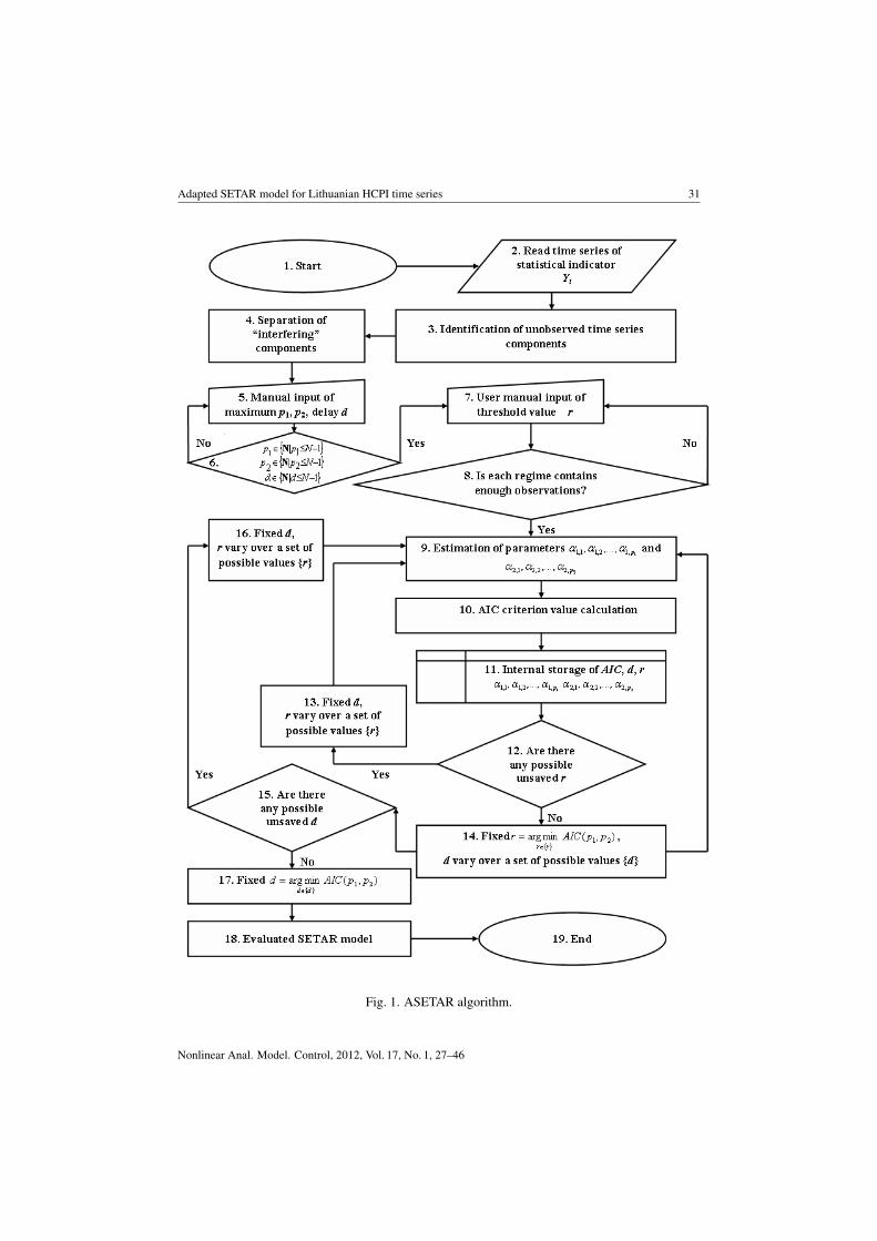
Important subject in adapted SETAR modelling is choosing an appropriate modelfrom a large set of candidate models. Proposed algorithm for model selection is presentedin Fig. 1. For simplicity of presentation, but without loss of generality, the details ofproposed algorithm are derived for a two-regime SETAR model in this section. Themethodology used is as follows:Steps 1–4. Before considering a series appropriate for modelling, several prior correctionsor adjustments may be needed. Most of real time series are affected by sudden unexpectedchanges, structural variations of the series that can only be observed on very long timeperiods, fluctuations observed during the year, which repeat themselves on a more or lessregular basis from one year to the other, or by other effects, that cannot be explained by themost commonly used time series models. First of all we propose to perform separation of“interfering” time series components for real time series Yt = Yt, t = 1, 2, . . . , N:

Yt = ω′tβ + C ′tη +

k∑j=1

ϕjλjIjt(tj) +

l∑i=1

Ut,i + yt. (2)

There ω′t = (ωt,1, . . . , ωt,n) denotes n regression or intervention variables, β = (β1, . . . ,βn)′ is a vector of regression coefficients,C ′t denotes the matrix with columns the calendar

effect variables (trading day, Easter effect, leap year effect, holidays), η is a vector ofassociated coefficients. It(tj) – an indicator variable for the possible presence of anoutlier at period tj , λj captures the transmission of the jth outlier effect and ϕj denotesthe coefficient of the outlier in the multiple regression model with k outliers. Ut,i is anunobserved time series components (seasonal component, trend or cycle), yt follows aSETAR process.

Parametric [13] or nonparametric methods [14] can be used for seasonal, trend orcycle component detection. Comparative analysis of these methods by using simulatedseries was done. This analysis showed that both methods are suitable for unobservedcomponents detection. In order not to expand the scope of this article the details of thisanalysis will not be described here.

Finally, before SETAR modelling, we suggest to test non-linearity for Yt and if it isconfirmed, then to check regime-switching nonlinearity.

Ramsey regression equation specification error test (RESET) can be chosen for non-linearity detection. The test is devised for a general form of misspecification. This isexecuted by estimating the following model:

y = φx+ φ1x2 + . . .+ φk−1x

k + ε, (3)

Nonlinear Anal. Model. Control, 2012, Vol. 17, No. 1, 27–46

30 N. Bratcikoviene

where x is an exploratory variables (autoregression variables in our case), φ, φ1, . . . , φkare parameters. Then testing null hypothesis whether φ1, . . . , φk are zero, by a meansof a F-test. If the null-hypothesis that all coefficients of the non-linear terms are zero isrejected, then the model has mis-specification.

RESET is popular test for identification of general form of nonlinearity. But it cannot answer to question whether this nonlinearity is threshold. Other tests for thresholdnonlinearity testing must be chosen. The class SETAR(1) is the class of linear autore-gressions. Thus testing for linearity (within the SETAR class of models) is a test of thenull hypothesis of SETAR(1) against the alternative of SETAR(m) for some m > 1.Testing linearity against the alternative of a SETAR model is discussed in [15] and [16].A solution is to use estimates of the SETAR model. F-statistic was proposed for testingof null hypothesis restrictions:

Fjk = N

(Sj − SkSk

), (4)

here Sj is the sum of squared residuals of SETAR(j) model (under the null hypothesis oflinearity) and accordingly Sk – of SETAR(k). For more details see [16].

Similarly null hypothesis of the SETAR(2) model versus alternative of SETAR(m) forsome m > 2 can be tested for right form of non-linearity identification. Scatterplots arealso informative tool for identification of nonlinearity and number of regimes.

Steps 5–6. User must to fix maximum model (p1, p2) and delay (d) parameters. Theycan not be larger than N − 1, there N is the modelled time series length and must besuch as to allow modelling of sufficient time series observations. Moreover model anddelay parameters can acquire only integer values. We recommend to take attention totime series length before fixing delay parameter. Choosing of quite small d is appropriatefor insufficiently long time series.

Steps 7–8. Threshold value r must be selected. The set of allowable threshold values rshould be such that each regime contains enough observations for the estimator definedabove to produce reliable estimates of autoregressive parameters. A popular choice ofr is to require that each regime contains at least a fraction π of the observations, that isr ∈ r|y[π(N−d)] ≤ r ≤ y[(1−π)(N−d)], where y(0), y(1), . . . , y(N−d) denote the orderstatistics of the threshold variable yN−d, y(0) ≤ y(1) ≤ . . . ≤ y(N−d) and [ · ] denotesinteger part. A safe choice for this fraction appears to be 0.15 [17].

Steps 9–17. These steps allow to locate the threshold value r and delay parameter dselected in the previous step. Threshold value r can vary over a set of possible valueswhile delay parameter d has to remain fixed. Then vice versa – r must be fixed and d canvary. Parameters are identified by calculating Akaike information criterion. (AIC). AIC isused and for a model selection. AIC is defined [9] as the sum of AIC’s for the AR modelsin the two regimes for two-regime SETAR model:

AIC(p1, p2) = n1lnσ21 + n2lnσ

22 + 2(p1 + 1) + 2(p2 + 1) (5)

there σ2j , j = 1, 2 is the variance of the residuals in the jth regime. AIC must attains its

minimum value for selected r and d.

www.mii.lt/NA


Fig. 1. ASETAR algorithm.


32 N. Bratcikoviene

Steps 18–19. Once the threshold value and delay parameter are fixed, the SETAR modelparameters can be estimated by using standard regression methods, for example ordinaryleast squares (OLS) method.

Assumption that the means and variances of variables are constant over the time withinregime must be done (otherwise OLS method may give misleading inferences). Thereforeunit root hypothesis must be tested within regimes before model parameters estimation.It is not necessary to test unit roots for Yt and yt, because unit root can be mistakenlyidentified in the presence of threshold determined regime switching (see [18]).

4 Out-of sample forecastingEstimating of forecasts from nonlinear models is considerably more complicated than es-timating from linear models. But there are some possibilities of out-of-sample forecastingof the nonlinear SETAR model: one-step-ahead, multi-step-ahead, the normal forecasterror, the Monte Carlo method, a special case of Monte Carlo method – the Skeletonmethod, the Bootstrap method and others. Comprehensive presentation of these methodsand forecasting results require quite a lot of space of this article. So we briefly outlineonly two forecasting methods: one-step-ahead and multi-step-ahead methods.

One-step-ahead method uses the only actual data for forecasting. It’s means that wedo not have to re-estimate the model every time when we added new data in the sampleseries. Denote

yt+1|t = E[yt+1 | Ωt] = F(yt;α

)(6)

as the optimal one-step-ahead forecast. Here F(yt;α) is nonlinear function whichfollows SETAR process (1),Ωt is the history of the time series up to observation at time t.

Estimation of more than one period ahead forecast rise some problems, because thelinear conditional expectation operator E can not be interchanged with the nonlinearoperator F (for more details see [17]).

The optimal h-step-ahead forecast can be obtained as

yt+h|t = E[yt+h | Ωt] = F(yt+h−1;α

)(7)

(see [18]). Original data and forecasted values of previous h − 1 periods are used forcalculation of forecast at time h.

5 Data and results5.1 Initial data and preadjustment

The series under this study are harmonised consumer price index (HCPI) by classifica-tion of individual consumption by purpose (COICOP/HICP) time series of Lithuania,covering the period from January of 1996 to December of 2009 (monthly data, 168observations). Time series frequency is monthly. A set of twelve HCPI index groupsare a subject to investigation of this article: Food and non-alcoholic beverages; Alcoholicbeverages, tobacco; Clothing and footwear; Housing, water, electricity, gas and otherfuels; Furnishings, household equipment and routine maintenance of the house; Health;

www.mii.lt/NA


Transport; Communication; Recreation and culture; Education; Restaurants and hotels;Miscellaneous goods and services. The natural logarithms of the original series wereanalysed. The data were obtained from the databases of statistics Lithuania.

Permanent changes took place in Lithuania’s economy over the past years. Most ofLithuanian time series have outliers, turning points, structural changes and breaks, sig-nificant seasonality. Accordingly, the time series of statistical indicators are complicatedboth in nature and their evaluation methods. Another problem with Lithuanian time seriesis that unfortunately they aren’t sufficiently long.

Due to these problems, as shown in the model selection algorithm, prior treatmentof time series is proposed before the SETAR modelling. Refusing of time series pre-adjustment can lead to model misspecification, biased parameter estimation. Importantpre-adjustments are the outlier correction and the removal of calendar effects.

Most of Lithuanian HCPI time series have significant outliers. All types of outliers(additive, transitory changes, level shifts) were fixed by using specific regression vari-ables (see [14]). Easter effect was significant only for index of Furnishings, householdequipment and routine maintenance of the house. A working day effect wasn’t signifi-cant for all HCPI time series. All HCPI series had significant seasonal component andfollowing by the proposed adapted SETAR model algorithm time series were detrendedand deseasonalized by using parametric method (see [13]) in the Step 3.

5.2 Empirical model selection results

In order to detect nonlinearities in HCPI, we performed the RESET test. It is composedfor the null hypothesis of linearity. It tests whether non-linear combinations of the es-timated values help explain the endogenous variable and if non-linear combinations ofthe explanatory variables have any power in explaining the endogenous variable, then themodel is mis-specified.

Table 1 reports the results of this test: value of RESET statistics and its p-value,powers (h) of the variables that should be included in the test and lag order under thenull hypothesis of linearity. The RESET test has been computed in the modified form.The modified RESET test requires that all the initial regressors enter linearly and up toa certain power h in the auxiliary regression (for details, see [19]). Only results with themost significant RESET statistic values are shown in Table 1.

As we mentioned above, RESET test is devised for general form of misspecificationand it can not detect threshold nonlinearity. For this purpose hypothesis of linear modelversus SETAR(2) was tested. Value of F-statistic test for linear model versus SETAR(2)are also presented in the Table 1. F-statistics for SETAR(3) models were not estimated,because analysed HCPI time series are sufficient short for SETAR(3) type modelling.

Nonlinearities in HCPI of Alcoholic beverages, tobacco, of Clothing and footwear,of Health, of Recreation and culture and of Restaurants and hotels time series werenot obtained by using RESET test. F test results are quite similar, except for Healthand Recreation and culture groups, where SETAR type nonlinearity are significant. Wedecided to use all HCPI time series for this study, on purpose to test adapted SETERmodels algorithm for such time series.


34 N. Bratcikoviene

Table 1. Nonlinearity test results.

HCPI group RESET p-value Power Lag F-statisticsstatistics order SETAR(1) vs

SETAR(2)01 Food and non-alcoholic beverages 8.4458 0.0042 2 1 14.152102 Alcoholic beverages, tobacco 2.0390 0.1553 3 8 3.836703 Clothing and footwear 2.6575 0.1051 3 11 3.836704 Housing, water, electricity,

gas and other fuels 6.5197 0.0117 2 12 10.492305 Furnishings, household equipment

and routine maintenance of the house 5.5619 0.0196 4 12 5.767006 Health 2.4429 0.1201 3 11 6.697407 Transport 5.1110 0.0251 2 1 7.166908 Communication 4.1340 0.0437 3 2 10.445209 Recreation and culture 2.0849 0.1508 2 11 8.370010 Education 7.2487 0.0078 2 1 21.634011 Restaurants and hotels 2.6015 0.1087 4 4 5.974012 Miscellaneous goods and services 4.6926 0.0318 2 1 8.2807

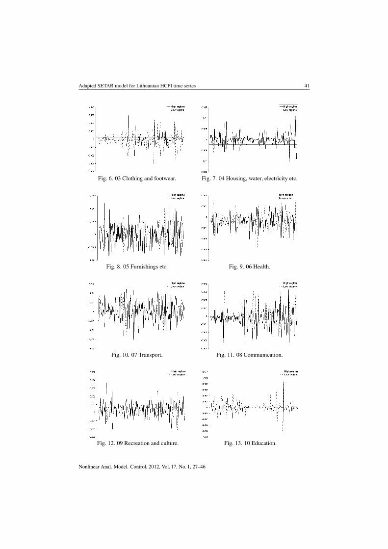
The selected SETAR model specifications are presented in Appendix A. The modelsshow clear evidence that Lithuanian HCPI by classification of individual consumptionby purpose time series are characterised by nonlinearities. Regime switching plots arepresented in Appendix B.

In order to compare the non-linear adapted SETAR model with a linear model, wechoose the ARIMA model to fit the data.

Box–Jenkins approach for building ARIMA models was used. ARIMA model iden-tification was made depending on autocorrelation function (ACF) and partial autocor-relation function (PACF). Models were selected by using Akaike information criterion.AIC was chosen for comparability and because our sample is quite small. Under unsta-ble conditions such as small sample and large noise levels Akaike information criterionoutperforms Bayesian information criteria (BIC) (see Acquah H., 2010). Residuals ofestimated models were tested for normality, Ljung-Box and Box-Pierce tests were doneand ACF/PACF also checked.

Nonlinearity of analysed time series were tested and parameters of SETAR andARIMA models were estimated using R package.

For model comparison we use the mean absolute percentage error (MAPE)

MAPE =1

N

N∑i=1

∣∣∣∣ yt − ytyt

∣∣∣∣ · 100 (8)

and root mean square prediction error (RMSPE)

RMSPE =

√√√√ 1

N

N∑i=1

(yt − ytyt

)2

· 100, (9)

www.mii.lt/NA


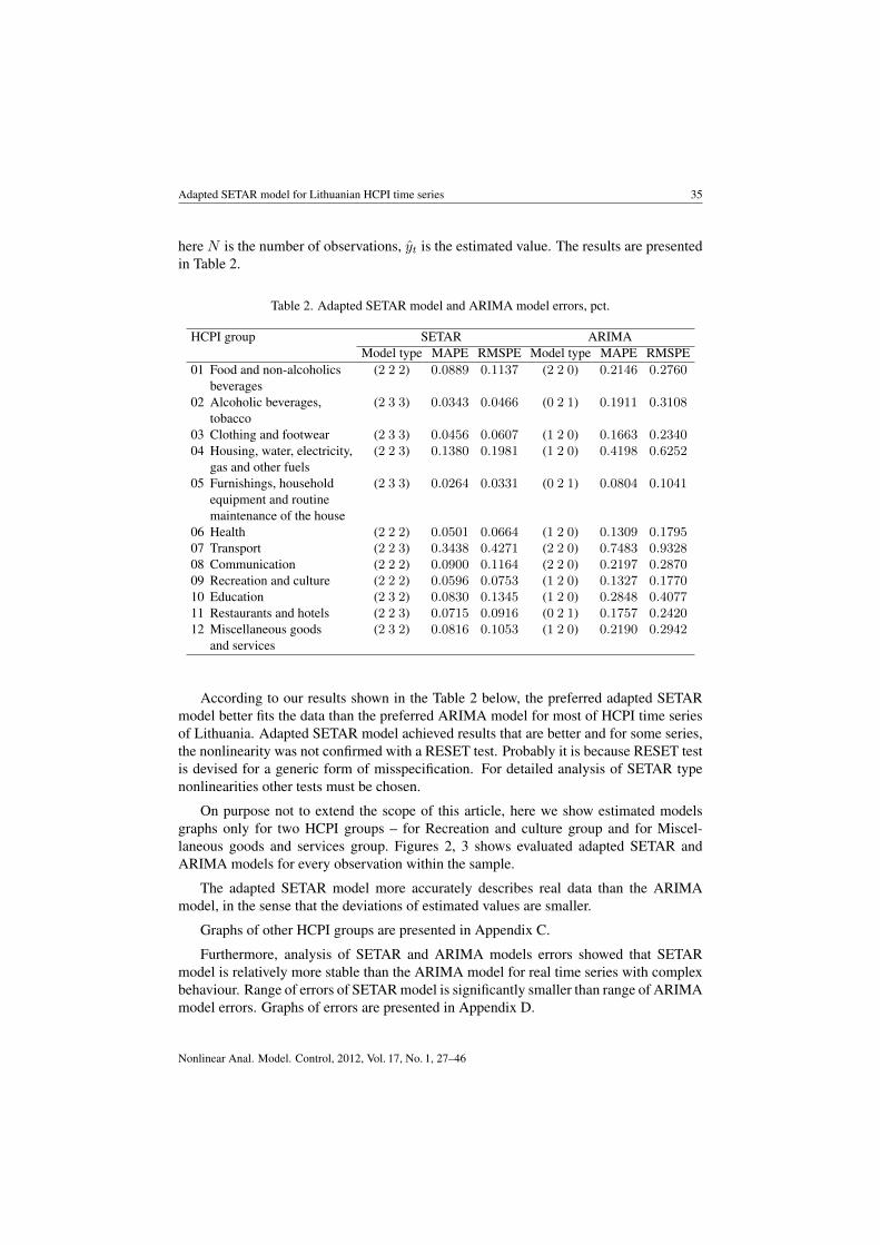
here N is the number of observations, yt is the estimated value. The results are presentedin Table 2.

Table 2. Adapted SETAR model and ARIMA model errors, pct.

HCPI group SETAR ARIMAModel type MAPE RMSPE Model type MAPE RMSPE

01 Food and non-alcoholics (2 2 2) 0.0889 0.1137 (2 2 0) 0.2146 0.2760beverages

02 Alcoholic beverages, (2 3 3) 0.0343 0.0466 (0 2 1) 0.1911 0.3108tobacco

03 Clothing and footwear (2 3 3) 0.0456 0.0607 (1 2 0) 0.1663 0.234004 Housing, water, electricity, (2 2 3) 0.1380 0.1981 (1 2 0) 0.4198 0.6252

gas and other fuels05 Furnishings, household (2 3 3) 0.0264 0.0331 (0 2 1) 0.0804 0.1041

equipment and routinemaintenance of the house

06 Health (2 2 2) 0.0501 0.0664 (1 2 0) 0.1309 0.179507 Transport (2 2 3) 0.3438 0.4271 (2 2 0) 0.7483 0.932808 Communication (2 2 2) 0.0900 0.1164 (2 2 0) 0.2197 0.287009 Recreation and culture (2 2 2) 0.0596 0.0753 (1 2 0) 0.1327 0.177010 Education (2 3 2) 0.0830 0.1345 (1 2 0) 0.2848 0.407711 Restaurants and hotels (2 2 3) 0.0715 0.0916 (0 2 1) 0.1757 0.242012 Miscellaneous goods (2 3 2) 0.0816 0.1053 (1 2 0) 0.2190 0.2942

and services

According to our results shown in the Table 2 below, the preferred adapted SETARmodel better fits the data than the preferred ARIMA model for most of HCPI time seriesof Lithuania. Adapted SETAR model achieved results that are better and for some series,the nonlinearity was not confirmed with a RESET test. Probably it is because RESET testis devised for a generic form of misspecification. For detailed analysis of SETAR typenonlinearities other tests must be chosen.

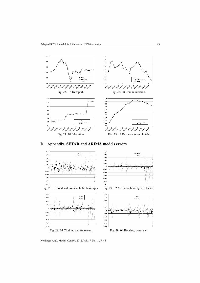
On purpose not to extend the scope of this article, here we show estimated modelsgraphs only for two HCPI groups – for Recreation and culture group and for Miscel-laneous goods and services group. Figures 2, 3 shows evaluated adapted SETAR andARIMA models for every observation within the sample.

The adapted SETAR model more accurately describes real data than the ARIMAmodel, in the sense that the deviations of estimated values are smaller.

Graphs of other HCPI groups are presented in Appendix C.

Furthermore, analysis of SETAR and ARIMA models errors showed that SETARmodel is relatively more stable than the ARIMA model for real time series with complexbehaviour. Range of errors of SETAR model is significantly smaller than range of ARIMAmodel errors. Graphs of errors are presented in Appendix D.


36 N. Bratcikoviene

Fig. 2. Evaluated models of recreation and culture HCPI.

Fig. 3. Evaluated models of miscellaneous goods and services HCPI.

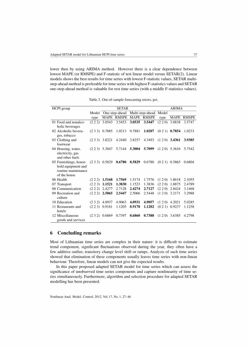
5.3 Out-of-sample forecasting results

As we mentioned above, one-step-ahead and multi-step-ahead methods were used for out-of -sample forecasting. Data were forecasted for 12 periods (one year) ahead. The resultswere compared with real monthly HCPI of 2010 year. ARIMA model forecasts were alsoestimated for comparison. MAPE and RSMPE of out-of-sample forecasting presented inTable 3 The lowest values of MAPE and RMSPE are in bold.

Results in the Table 3 shows that there are no strong differences between the out-of-sample forecasting methods errors, but better ARIMA forecasts obtained only for onetime series – Clothing and footwear. MAPE of Alcoholic beverages, tobacco time seriesforecasts is lower by using ARIMA, but RMSPE is lower by using SETAR multi-step-ahead method. Greatest difference is seen in miscellaneous goods and services time series– errors obtained by using SETAR multi-step-ahead methods are more than five times

www.mii.lt/NA


lower then by using ARIMA method. However there is a clear dependence betweenlowest MAPE (or RMSPE) and F-statistic of test linear model versus SETAR(2). Linearmodels shows the best results for time series with lowest F-statistic values, SETAR multi-step-ahead method is preferable for time series with highest F-statistics values and SETARone-step-ahead method is valuable for rest time series (with a middle F-statistics values).

Table 3. Out-of-sample forecasting errors, pct.

HCPI group SETAR ARIMAModel One-step-ahead Multi-step-ahead Modeltype MAPE RMSPE MAPE RMSPE type MAPE RMSPE

01 Food and nonalco- (2 2 2) 3.0543 3.5453 3.0535 3.5447 (2 2 0) 3.0838 3.5747holic beverages

02 Alcoholic bevera- (2 3 3) 0.7885 1.0213 0.7881 1.0207 (0 2 1) 0.7854 1.0233ges, tobacco

03 Clothing and (2 3 3) 3.8221 4.2440 3.8257 4.3493 (1 2 0) 3.4361 3.9385footwear

04 Housing, water, (2 2 3) 5.3047 5.7144 5.3004 5.7099 (1 2 0) 5.3616 5.7542electricity, gasand other fuels

05 Furnishings, house- (2 3 3) 0.5829 0.6780 0.5829 0.6780 (0 2 1) 0.5865 0.6804hold equipment androutine maintenanceof the house

06 Health (2 2 2) 1.5168 1.7569 1.5174 1.7576 (1 2 0) 1.8618 2.105507 Transport (2 2 3) 1.1521 1.3830 1.1523 1.3836 (2 2 0) 1.8875 2.478908 Communication (2 2 2) 2.4277 2.7128 2.4274 2.7127 (2 2 0) 2.8424 3.146809 Recreation and (2 2 2) 2.5065 2.5447 2.5066 2.5448 (1 2 0) 3.2171 3.2988

culture10 Education (2 3 2) 4.0937 4.9063 4.0931 4.9057 (1 2 0) 4.2021 5.028511 Restaurants and (2 2 3) 0.9181 1.1205 0.9178 1.1202 (0 2 1) 0.9237 1.1258

hotels12 Miscellaneous (2 3 2) 0.6869 0.7397 0.6860 0.7388 (1 2 0) 3.6385 4.2798

goods and services

6 Concluding remarks

Most of Lithuanian time series are complex in their nature: it is difficult to estimatetrend component, significant fluctuations observed during the year, they often have afew additive outlier, transitory change level shift or ramps. Analysis of such time seriesshowed that elimination of these components usually leaves time series with non-linearbehaviour. Therefore, linear models can not give the expected results.

In this paper proposed adapted SETAR model for time series which can assess thesignificance of unobserved time series components and capture nonlinearity of time se-ries simultaneously. Furthermore, algorithm and selection procedure for adapted SETARmodelling has been presented.


38 N. Bratcikoviene

Considering the nonlinearities of Lithuanian HCPI time series the adapted SETARmodel was proposed for modelling of these time series. Estimated results are comparedwith a standard ARIMA model. The adapted SETAR model have a good in-sample andout-of-sample fit compared to linear models and performs more accurate modelling resultsfor most of analysed time series. A practical example shows that the proposed algorithmallows for a relatively accurate description of time series with difficult structure. The pro-posed model is appropriate to use in modelling of real time series with complex behaviour.

A Appendix. Models specification

Table 4. SETAR models specification.

SETARCoefficients t-value

01 Food and non-alcoholic beveragesr = −0.001321, d = 1Residuals: σ2 = 1.456e− 06, AIC = −2236

Regime 1 α1,0 0.0012039480 3.5962α1,1 −0.6083981450 −4.1591

Regime 2 α2,0 −0.0002239026 −2.1248α2,1 −0.6761263532 −8.5952

02 Alcoholic beverages, tobaccor = −0.0008643, d = 1Residuals: σ2 = 2.831e− 07, AIC = −2506

Regime 1 α1,0 −0.0002057731 −0.7124α1,1 −1.6221727546 −9.2993α1,2 −1.0618182104 −5.5055

Regime 2 α2,0 −3.456317e−05 −0.7109α2,1 −9.655383e−01 −13.1450α2,2 −2.547517e−01 −3.1458

03 Clothing and footwearr = 0.0002846, d = 1Residuals: σ2 = 3.181e− 07, AIC = −2486

Regime 1 α1,0 −0.0001012661 −1.5988α1,1 −0.8752428211 −11.1250α1,2 −0.4306680029 −4.2287

Regime 2 α2,0 −0.0002173414 −1.4592α2,1 −1.0163095643 −7.2433α2,2 −0.5135607943 −3.2459

04 Housing, water, electricity, gas and other fuelsr = −0.002226, d = 1Residuals: σ2 = 3.781e− 06, AIC = −2075

Regime 1 α1,0 0.0024159830 4.6720α1,1 −0.6445811930 −4.6469

www.mii.lt/NA



Regime 2 α2,0 −0.0001112684 −0.6347α2,1 −0.8126394166 −11.1550α2,2 −0.5158333462 −6.1125

05 Furnishings, household equipmentand routine maintenance of the houser = −0.0002725, d = 1Residuals: σ2 = 1.103e− 07, AIC = −2663

Regime 1 α1,0 −0.0001126799 −0.8281α1,1 −0.6275533966 −4.6399α1,2 −0.5199540370 −2.1064

Regime 2 α2,0 −2.383143e−05 −0.6469α2,1 −7.950423e−01 −9.0729α2,2 −2.685457e−01 −2.5776

06 Healthr = −0.0004662, d = 0Residuals: σ2 = 4.361e− 07, AIC = −2438

Regime 1 α1,0 −0.0003329224 −1.8259α1,1 −0.3108870673 −1.6835

Regime 2 α2,0 −0.0004793827 −3.8626α2,1 −0.5314376157 −7.0065

07 Transportr = −0.004508, d = 1Residuals: σ2 = 1.683e− 05, AIC = −1826

Regime 1 α1,0 0.0044665070 4.4104α1,1 −0.5742683750 −2.9868

Regime 2 α2,0 0.0003811062 0.9805α2,1 −0.6748489982 −8.9148α2,2 −0.4327181118 −4.3506

08 Communicationr = −0.001198, d = 0Residuals: σ2 = 1.217e− 06, AIC = −2266

Regime 1 α1,0 −0.0020796470 −2.7685α1,1 −1.1665765320 −3.4192

Regime 2 α2,0 −0.0001881815 −1.9643α2,1 −0.4659240738 −4.8597

09 Recreation and culturer = −0.0005073, d = 0Residuals: σ2 = 6.027e− 07, AIC = −2384

Regime 1 α1,0 −0.0004371123 −1.1773α1,1 −1.2622289072 −3.6243


40 N. Bratcikoviene


Regime 2 α2,0 0.0006235662 6.9811α2,1 −0.4734874292 −5.0142

10 Educationr = 0.0004024, d = 1Residuals: σ2 = 1.980e− 06, AIC = −2183

Regime 1 α1,0 0.0001074849 0.7230α1,1 −0.6612599177 −8.4164α1,2 −0.3715715094 −3.1676

Regime 2 α2,0 −0.000623708 −2.7291α2,1 −0.124767848 −0.8233

11 Restaurants and hotelsr = −0.0001142, d = 0Residuals: σ2 = 8.389e− 07, AIC = −2327

Regime 1 α1,0 −1.818863e−05 −0.0919α1,1 −6.098142e−01 −4.1601

Regime 2 α2,0 0.0003628096 2.6768α2,1 −0.9513979917 −7.3238α2,2 −0.4500337286 −5.2651

12 Miscellaneous goods and servicesr = 0.0007705, d = 1Residuals: σ2 = 1.052e− 06, AIC = −2289

Regime 1 α1,0 0.0003265502 3.0956α1,1 −0.6114431815 −7.6719α1,2 −0.4733193410 −4.1515

Regime 2 α2,0 −0.0005396149 −3.3403α2,1 −0.4003480709 −2.8540

B Appendix. Regime switching plots

Fig. 4. 01 Food and non-alcoholic beverages. Fig. 5. 02 Alcoholic beverages, tobacco.

www.mii.lt/NA


Fig. 6. 03 Clothing and footwear. Fig. 7. 04 Housing, water, electricity etc.

Fig. 8. 05 Furnishings etc. Fig. 9. 06 Health.

Fig. 10. 07 Transport. Fig. 11. 08 Communication.

Fig. 12. 09 Recreation and culture. Fig. 13. 10 Education.


42 N. Bratcikoviene

Fig. 14. 11 Restaurants and hotels. Fig. 15. Miscellaneous goods and services.

C Appendix. Evaluated adapted SETAR and ARIMA models


Fig. 18. 03 Clothing and footwear. Fig. 19. 04 Housing, water, electricity etc.


www.mii.lt/NA



Fig. 24. 10 Education. Fig. 25. 11 Restaurants and hotels.

D Appendix. SETAR and ARIMA models errors


Fig. 28. 03 Clothing and footwear. Fig. 29. 04 Housing, water etc.


44 N. Bratcikoviene



Fig. 34. 09 Recreation and culture. Fig. 35. 10 Education.

Fig. 36. 11 Restaurants and hotels. Fig. 37. 12 Miscellaneous goods and services.

www.mii.lt/NA


References

1. J. Bai, P.Perron, Estimating and testing linear models with multiple structural changes,Econometrica, 66, pp. 47–78, 1998.

2. S.E. Culver, D.H. Papell, Is there a unit root in the inflation rate? Evidence from sequentialbreak and panel data models, J. Appl. Econom., 12, pp. 435–444, 1997.

3. J. Emerson, K. Chihwa, Testing for structural change in panel data: GDP growth, consumptiongrowth, and productivity growth, Economics Bulletin, 3(14), pp. 1–12, 2006.

4. P. Perron, Q. Zhongjun, Estimating and testing structural changes in multivariate regressions,Econometrica, 75(2), pp. 459–502, 2007.

5. Ch. Chatfield, The Analysis of Time Series: An Introduction, CRC Press, Boca Raton, FL, 2004.

6. D.W. Bacon, D.G. Watts, Estimating the transition between two intersecting lines, Biometrica,58, pp. 525–534, 1971.

7. H. Tong, On a threshold model, in: C.H. Chen (Ed.), Pattern Recognition and Signal Proces-sing, Sijthoff and Noordhoff, Amsterdam, 1978, pp. 101–141.

8. H. Tong, Threshold Models in Non-Linear Time Series Analysis, Springer-Verlag, New York,1983.

9. H. Tong, Non-Linear Time Series: A Dynamical Systems Approach, Oxford Univ. Press,Oxford, 1990.

10. H. Tong, A personal overview of non-linear time series analysis from a chaos perspective,Scand. J. Stat., 22, pp. 299–445, 1995.

11. B. Siliverstovs, D. Dijk, Forecasting industrial production with linear, nonlinear, and structuralchange models, Econometric Institute Report, No. EI 2003-16, Erasmus School of Economics,Rotterdam, 2003.

12. J. Öhrvic, G. Schoier, SETAR model selection – A Bootstrap approach, Comput. Stat., 20(4),pp. 559–573, 2005.

13. V. Gòmez, A. Maravall, Seasonal adjustment and signal extraction in economic time series, in:A Course in Time Series Analysis, J. Wiley, New York, 2001, Chapt. 8, pp. 202–247.

14. D.F. Findley, B.C. Monsell, W.R. Bell, M.C. Otto, B.Ch. Chen, New capabilities and methodsof the X-12-ARIMA seasonal adjustment program, J. Bus. Econ. Stat., 16(2), pp. 127–152,1998.

15. K.S. Chan, Testing for threshold autoregression, Ann. Stat., 18, pp. 1886–1894, 1990.

16. E.H. Hansen, Testing for linearity, Journal of Economic Surveys, 13(5), pp. 551–575, 1999.

17. P.H. Franses, D. van Dijk, Non-Linear Time Series Models in Empirical Finance, CambridgeUniv. Press, Cambridge, 2000.

18. H. Feng, J. Liu, A SETAR model for canadian GDP: Non-linearities and forecast comparisons,Appl. Econ., 35(18), pp. 1957–1964, 2003.


46 N. Bratcikoviene

19. J.G. Thursby, P. Schmidt, Some properties of tests for the specification error in a linearregression model, J. Am. Stat. Assoc., 72, pp. 635–641, 1977.

20. A.F. Burns, W.C. Mitchell, Measuring Business Cycles, National Bureau of EconometricResearch, New York, 1946.

21. R. Dacco, S. Satchell, Why do regime-switching models forecast so badly?, J. Forecast., 18,pp. 1–16, 1999.

22. W. Mitchell, Business Cycles: The Problem and Its Setting, National Bureau of EconometricResearch, New York, 1927.

23. R.S. Tsay, Testing and modelling threshold autoregressive processes, J. Am. Stat. Assoc.,84(405), pp. 231–240, 1989.

www.mii.lt/NA

Adapted SETAR model for Lithuanian HCPI time … · Nonlinear Analysis: Modelling and Control,...

Documents

Transcript of Adapted SETAR model for Lithuanian HCPI time … · Nonlinear Analysis: Modelling and Control,...