ADA Compliant Lecture PowerPoint - Yulin Hou · As the price of pizza falls and the budget...
34
Copyright © 2017 Pearson Education, Inc. All Rights Reserved Economics 6 th edition Chapter 10 Consumer Choice and Behavioral Economics Modified by Yulin Hou For Principles of Microeconomics Florida International University Fall 2017 1
Transcript of ADA Compliant Lecture PowerPoint - Yulin Hou · As the price of pizza falls and the budget...

Copyright © 2017 Pearson Education, Inc. All Rights Reserved
Economics6th edition
Chapter 10
Consumer Choice and Behavioral
Economics
Modified by Yulin Hou
For Principles of Microeconomics
Florida International University
Fall 2017
1

Copyright © 2017 Pearson Education, Inc. All Rights Reserved
Utility: measuring happiness
Economists refer to the enjoyment or satisfaction that people
obtain from consuming goods and services as utility.
Utility cannot be directly measured; but for now, suppose that it
could. What would we see?
• As people consumed more of an item (say, pizza) their total
utility would change.
The amount by which total utility would change when consuming
an extra unit of a good or service is called the marginal utility
(MU).
• Remember: in economics, “marginal” means “additional”.
2
Copyright © 2017 Pearson Education, Inc. All Rights Reserved
Diminishing marginal utility and budgets
We generally expect to see the first items consumed produce the
most marginal utility, so that subsequent items give diminishing
marginal utility.
Law of diminishing marginal utility: The principle that
consumers experience diminishing additional satisfaction as they
consume more of a good or service during a given period of time.
3

Copyright © 2017 Pearson Education, Inc. All Rights Reserved
Figure 10.1 Total and marginal utility from eating pizza on
Super Bowl Sunday (1 of 2)
The table shows the total utility
you might derive from eating
pizza on Super Bowl Sunday.
The numbers, in utils, represent
happiness: higher is better.
A graph of this utility is initially
rising quickly, then more slowly;
and eventually, it turns
downward (as you get sick of
pizza).
4

Copyright © 2017 Pearson Education, Inc. All Rights Reserved
Figure 10.1 Total and marginal utility from eating pizza on
Super Bowl Sunday (2 of 2)
The increase in utility from one
slice to the next is the marginal
utility of a slice of pizza.
We can calculate marginal
utility for every slice of pizza…
… then graph the results. The
graph of marginal utility is
decreasing, showing the Law of
Diminishing Marginal Utility
directly.
5

Copyright © 2017 Pearson Education, Inc. All Rights Reserved
Allocating your resources
Given unlimited resources, a consumer would consume every
good and service up until the maximum total utility.
• But resources are scarce; consumers have a budget constraint.
Budget constraint: The limited amount of income available to
consumers to spend on goods and services.
The concept of utility can help us figure out how much of each
item to purchase.
• Each item purchased gives some (possibly negative) marginal
utility; by dividing by the price of the item, we obtain the
marginal utility per dollar spent; that is, the rate at which that
item allows the consumer to transform money into utility.
6
Copyright © 2017 Pearson Education, Inc. All Rights Reserved
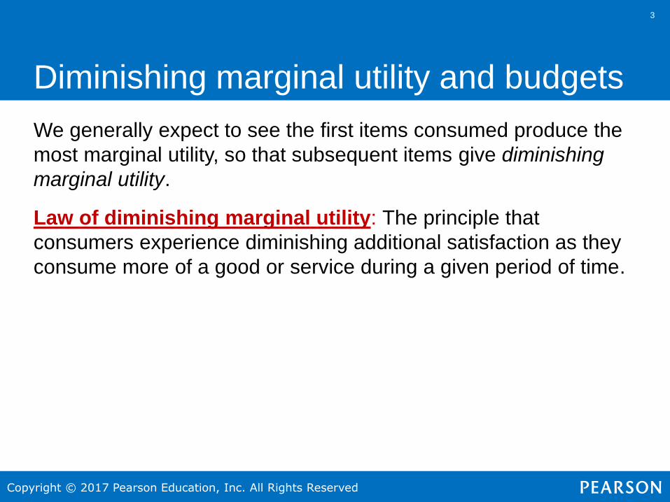
Table 10.1 Total utility and marginal utility from eating pizza
and drinking Coke
Suppose you can now obtain utility by eating pizza and drinking
Coke.
The table gives the total and marginal utility derived from each
activity.
7

Copyright © 2017 Pearson Education, Inc. All Rights Reserved
Table 10.2 Converting marginal utility to marginal utility per
dollar
Suppose that pizza costs $2 per slice, and Coke $1 per cup.
• Marginal utility of pizza per dollar is just marginal utility of pizza
divided by the price, $2.
• Similarly for Coke: divide by $1.
8

Copyright © 2017 Pearson Education, Inc. All Rights Reserved
Table 10.3 Equalizing marginal utility per dollar spent (1 of 2)
Suppose the marginal utility per dollar obtained from pizza was
greater than that obtained from Coke.
• Then you should eat more pizza, and drink less Coke.
This implies the Rule of Equal Marginal Utility per Dollar Spent:
consumers should seek to equalize the “bang for the buck”.
• Some combinations satisfying this rule are given above.
9
Copyright © 2017 Pearson Education, Inc. All Rights Reserved
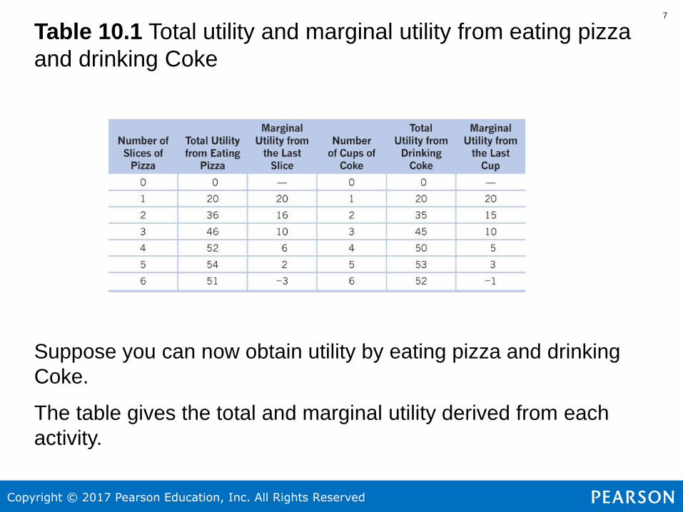
Table 10.3 Equalizing marginal utility per dollar spent (2 of 2)
The actual combination to purchase would depend on your budget
constraint:
• With $5 to spend, you would purchase 1 slice of pizza and 3
cups of Coke.
• With $10 to spend, you would purchase 3 slices of pizza and 4
cups of Coke.
In each case, you seek to exhaust your budget, since spending
additional money gives more utility.
10

Copyright © 2017 Pearson Education, Inc. All Rights Reserved
Conditions for maximizing utility
This gives us two conditions for maximizing utility:
1. Satisfy the Rule of Equal Marginal Utility per Dollar Spent:
𝑀𝑈𝑃𝑖𝑧𝑧𝑎𝑃𝑃𝑖𝑧𝑧𝑎
=𝑀𝑈𝐶𝑜𝑘𝑒𝑃𝐶𝑜𝑘𝑒
2. Exhaust your budget:
Spending on pizza + Spending on Coke = Budget
11

Copyright © 2017 Pearson Education, Inc. All Rights Reserved
What if prices change?
If the price of pizza changes from $2 to $1.50, then the Rule of
Equal Marginal Utility per Dollar Spent will no longer be satisfied.
• You must adjust your purchasing decision.
We can think of this adjustment in two ways:
1. You can afford more than before; this is like having a higher
income.
2. Pizza has become cheaper relative to Coke.
We refer to the effect from 1. as the income effect, and the effect
from 2. as the substitution effect.
12
Copyright © 2017 Pearson Education, Inc. All Rights Reserved
1. Income effect
Income effect: The change in the quantity demanded of a good
that results from the effect of a change in price on consumer
purchasing power, holding all other factors constant.
We know that some goods are normal (goods that we consume
more of as our income rises) and some are inferior (goods that we
consume less of as our income rises).
• If pizza is a normal good, the income effect of its price
decreasing will cause you to consume more pizza.
• If pizza is an inferior good, the income effect of its price
decreasing will cause you to consume less pizza.
13

Copyright © 2017 Pearson Education, Inc. All Rights Reserved
2. Substitution effect
Substitution effect: The change in the quantity demanded of a
good that results from a change in price making the good more or
less expensive relative to other goods, holding constant the effect
of the price change on consumer purchasing power.
If the price of pizza falls, pizza becomes cheaper relative to Coke.
• The opportunity cost of consuming a slice of pizza falls.
• This suggests eating more pizza.
14

Copyright © 2017 Pearson Education, Inc. All Rights Reserved
Income effect and substitution effect of a price change
The table summarizes the income and substitution effects.
15
Copyright © 2017 Pearson Education, Inc. All Rights Reserved
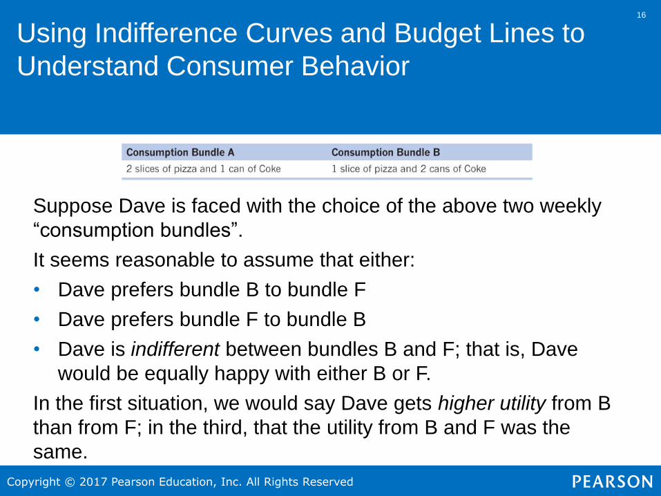
Using Indifference Curves and Budget Lines to
Understand Consumer Behavior
Suppose Dave is faced with the choice of the above two weekly
“consumption bundles”.
It seems reasonable to assume that either:
• Dave prefers bundle B to bundle F
• Dave prefers bundle F to bundle B
• Dave is indifferent between bundles B and F; that is, Dave
would be equally happy with either B or F.
In the first situation, we would say Dave gets higher utility from B
than from F; in the third, that the utility from B and F was the
same.
16
Copyright © 2017 Pearson Education, Inc. All Rights Reserved
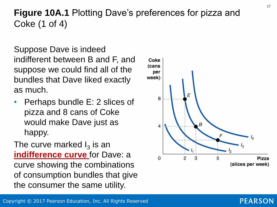
Figure 10A.1 Plotting Dave’s preferences for pizza and
Coke (1 of 4)
Suppose Dave is indeed
indifferent between B and F, and
suppose we could find all of the
bundles that Dave liked exactly
as much.
• Perhaps bundle E: 2 slices of
pizza and 8 cans of Coke
would make Dave just as
happy.
The curve marked I3 is an
indifference curve for Dave: a
curve showing the combinations
of consumption bundles that give
the consumer the same utility.
17

Copyright © 2017 Pearson Education, Inc. All Rights Reserved
Figure 10A.1 Plotting Dave’s preferences for pizza and
Coke (2 of 4)
Lower indifference curves
represent lower levels of utility;
higher indifference curves
represent higher levels of utility.
Bundle A is on I1, a lower
indifference curve; and it is
clearly worse than E, B, or F,
since it has less pizza and Coke
than any of those bundles.
Bundle C is on a higher
indifference curve, and is clearly
better than B (more pizza and
Coke).
18
Copyright © 2017 Pearson Education, Inc. All Rights Reserved
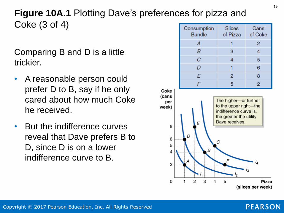
Figure 10A.1 Plotting Dave’s preferences for pizza and
Coke (3 of 4)
Comparing B and D is a little
trickier.
• A reasonable person could
prefer D to B, say if he only
cared about how much Coke
he received.
• But the indifference curves
reveal that Dave prefers B to
D, since D is on a lower
indifference curve to B.
19
Copyright © 2017 Pearson Education, Inc. All Rights Reserved
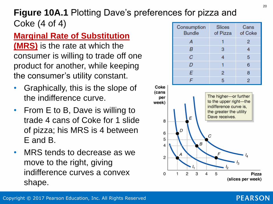
Figure 10A.1 Plotting Dave’s preferences for pizza and
Coke (4 of 4)
Marginal Rate of Substitution
(MRS) is the rate at which the
consumer is willing to trade off one
product for another, while keeping
the consumer’s utility constant.
• Graphically, this is the slope of
the indifference curve.
• From E to B, Dave is willing to
trade 4 cans of Coke for 1 slide
of pizza; his MRS is 4 between
E and B.
• MRS tends to decrease as we
move to the right, giving
indifference curves a convex
shape.
20
Copyright © 2017 Pearson Education, Inc. All Rights Reserved
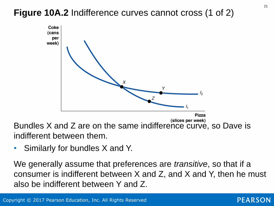
Figure 10A.2 Indifference curves cannot cross (1 of 2)
Bundles X and Z are on the same indifference curve, so Dave is
indifferent between them.
• Similarly for bundles X and Y.
We generally assume that preferences are transitive, so that if a
consumer is indifferent between X and Z, and X and Y, then he must
also be indifferent between Y and Z.
21

Copyright © 2017 Pearson Education, Inc. All Rights Reserved
Figure 10A.2 Indifference curves cannot cross (2 of 2)
But Dave will prefer Y to Z, since Y has more pizza and Coke.
Since transitivity is such an intuitively sensible assumption, we
conclude that indifference curves will never cross.
22

Copyright © 2017 Pearson Education, Inc. All Rights Reserved
Figure 10A.3 Dave’s budget constraint
A consumer’s budget constraint
is the amount of income he or
she has available to spend on
goods and services.
The table shows bundles Dave
can buy with $10, if pizza costs
$2 per slice and Coke costs $1
per can.
The slope of the budget
constraint is the (negative of the)
ratio of prices; it represents the
rate at which Dave is allowed to
trade Coke for pizza: 2 cans of
Coke per 1 slice of pizza.
23
Copyright © 2017 Pearson Education, Inc. All Rights Reserved
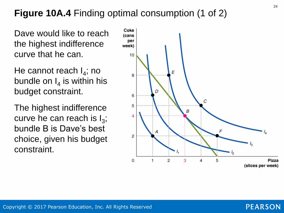
Figure 10A.4 Finding optimal consumption (1 of 2)
Dave would like to reach
the highest indifference
curve that he can.
He cannot reach I4; no
bundle on I4 is within his
budget constraint.
The highest indifference
curve he can reach is I3;
bundle B is Dave’s best
choice, given his budget
constraint.
24

Copyright © 2017 Pearson Education, Inc. All Rights Reserved
Figure 10A.4 Finding optimal consumption (2 of 2)
To maximize utility, a
consumer needs to be
on the highest
indifference curve, given
his budget constraint.
Notice that at this point,
the indifference curve is
just tangent to the
budget line.
25

Copyright © 2017 Pearson Education, Inc. All Rights Reserved
Figure 10A.5 How a price decrease affects the budget
constraint
When the price of
pizza falls, Dave can
buy more pizza than
before.
If pizza falls to $1.00 per
slice, Dave can buy 10
slices of pizza per week;
he can still afford 10
cans of Coke per week.
The budget constraint
rotates out along the
pizza-axis to reflect this
increase in purchasing
power.
26

Copyright © 2017 Pearson Education, Inc. All Rights Reserved
Figure 10A.6 How a price
change affects optimal
consumption
As the price of pizza falls
and the budget constraint
rotates out, Dave’s optimal
bundle will change.
When pizza cost $2.00 per
slice, Dave bought 3 slices.
• Now that pizza costs
$1.00 per slice, Dave
buys 7 slices.
These are two points on
Dave’s demand curve for
pizza (assuming he has $10,
and Coke costs $1 per can).
27

Copyright © 2017 Pearson Education, Inc. All Rights Reserved
Figure 10A.7 Income and substitution effects of a price
change (1 of 2)
When the price of pizza
falls, Dave changes his
consumption from A to C.
We can think of this as
two separate effects:
1. A change in relative
price keeping utility
constant, causing a
movement along
indifference curve I1;
this is the substitution
effect.
28

Copyright © 2017 Pearson Education, Inc. All Rights Reserved
Figure 10A.7 Income and substitution effects of a price
change (2 of 2)
When the price of pizza
falls, Dave changes his
consumption from A to C.
We can think of this as
two separate effects:
2. An increase in
purchasing power,
causing a movement
from B to C; this is the
income effect.
29

Copyright © 2017 Pearson Education, Inc. All Rights Reserved
Figure 10A.8 How a change in income affects the budget
constraint
When the income Dave
has to spend on pizza
and Coke increases from
$10 to $20, his budget
constraint shifts outward.
With $10, Dave could buy
a maximum of 5 slices of
pizza or 10 cans of Coke.
With $20, he can buy a
maximum of 10 slices of
pizza or 20 cans of Coke.
30

Copyright © 2017 Pearson Education, Inc. All Rights Reserved
Figure 10A.9 How a change in income affects optimal
consumption
An increase in income
leads Dave to consume
more Coke…
… and more pizza.
For Dave, both Coke and
pizza are normal goods.
A different consumer might
have different preferences,
and an increase in income
might decrease the
demand for Coke, for
example; in this case, Coke
would be an inferior good.
31

Copyright © 2017 Pearson Education, Inc. All Rights Reserved
Figure 10A.10 At the optimum point, the slopes of the
indifference curve and the budget constraint are the same
32

Copyright © 2017 Pearson Education, Inc. All Rights Reserved
Relating MRS and marginal utility
Suppose Dave is indifferent between two bundles, A and B. A has
more Coke than B, so B must have more pizza than A.
As Dave moves from A to B, the loss (in utility) from consuming
less coke must be just offset by the gain (in utility) from consuming
more pizza. We can write:− Change in the quantity of Coke × 𝑀𝑈𝐶𝑜𝑘𝑒 = Change in the quantity of pizza × 𝑀𝑈𝑃𝑖𝑧𝑧𝑎
Rearranging terms gives:−Change in the quantity of Coke
Change in the quantity of pizza=𝑀𝑈𝑃𝑖𝑧𝑧𝑎𝑀𝑈𝐶𝑜𝑘𝑒
And this first term is the slope of the indifference curve: the MRS.−Change in the quantity of Coke
Change in the quantity of pizza= 𝑀𝑅𝑆 =
𝑀𝑈𝑃𝑖𝑧𝑧𝑎𝑀𝑈𝐶𝑜𝑘𝑒
33
Copyright © 2017 Pearson Education, Inc. All Rights Reserved
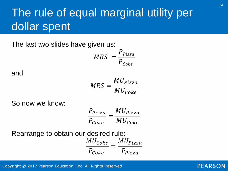
The rule of equal marginal utility per
dollar spent
The last two slides have given us:
𝑀𝑅𝑆 =𝑃𝑃𝑖𝑧𝑧𝑎
𝑃𝐶𝑜𝑘𝑒
and
𝑀𝑅𝑆 =𝑀𝑈𝑃𝑖𝑧𝑧𝑎𝑀𝑈𝐶𝑜𝑘𝑒
So now we know:𝑃𝑃𝑖𝑧𝑧𝑎𝑃𝐶𝑜𝑘𝑒
=𝑀𝑈𝑃𝑖𝑧𝑧𝑎𝑀𝑈𝐶𝑜𝑘𝑒
Rearrange to obtain our desired rule:𝑀𝑈𝐶𝑜𝑘𝑒𝑃𝐶𝑜𝑘𝑒
=𝑀𝑈𝑃𝑖𝑧𝑧𝑎𝑃𝑃𝑖𝑧𝑧𝑎
34