AD-Al109 627 ANALYSIS AND TECHHOLOGM INC NORTH …
129
AD-Al109 627 ANALYSIS AND TECHHOLOGM INC NORTH STONINGTON CT F/B 12/1 TARGET NO0TION ANALYSIS WITH A PRIORI INFORAION.(W) OCT 8!2 C B BILLING, H F .JARVIS NOO1-SO.C-O379 UNCLASSIFIED P-5,5 -B1N
Transcript of AD-Al109 627 ANALYSIS AND TECHHOLOGM INC NORTH …

AD-Al109 627 ANALYSIS AND TECHHOLOGM INC NORTH STONINGTON CT F/B 12/1TARGET NO0TION ANALYSIS WITH A PRIORI INFORAION.(W)OCT 8!2 C B BILLING, H F .JARVIS NOO1-SO.C-O379
UNCLASSIFIED P-5,5 -B1N

fig ~ I,~ ( 112. 211111 -I.V _ 1I11l1 111112.0
11111!.2 -A Iiu
MICROCOPY RESOLUTION TEST CHART
NATIONAL RUL9AU (A ',TAN[)ARD)S i(3 A

' OPERATIONS RESEARCH
SYSTEMS ENGINEERING
SYSTEMS ANALYSIS
OCEAN SCIENCES - 1c
SIMULATION A
ANALYTICAL MODELING
L This dovier ni.t has been appo vd
fox pblic releaze and sale itdi-t ibutiMn is unlimited.
COMPUTER SCIENCES
82 01 13 071

I mI ANALYSIS TECHNOLOGY
TARGET MOTION ANALYSISWITH
A PRIORI
I NFORMAT ION
Analysis & Technology, Inc.Report No. P-515-2-81
Contract N00014-80-C-0379Task Number (NR 274-302)
19 October 1981 T IC
Prepared by:
Clare B. Billing, Jr.Harold F. Jarvis, Jr.
Approved by: c 2-.,T. M. Downie, ManagerSystems Research &
Analysis Dept.
Prepared for:
Office of Naval Research800 No. Quincy StreetArlington, VA 22217
(Attn: Mr. James G. Smith, Code 411 S&P)
REPRODUCTION IN WHOLE OR IN PART IS APPROVED FOR PUBLIC RELEASE;PERMITTED FOR ANY PURPOSE OF THE DISTRIBUTION UNLIMITEDUNITED STATES GOVERNMENT
Analysis & Technology, Inc. - Technology Park, P. 0. Box 220, North Stonington, Connecticut 06359 - (203) 599-3910

UNCLASSIFIEDSECURITY CLASSIFICATION6 OF THIS PAGE (fte Does Ener~)
REPORT DOCUMENTATION PAGE EFRE" COMPETIN OR
1. REPORT HUMSER 2. GOVT ACCESSION NO 0. RECIPIENT'S CATALOG NUMERM
4. TITLE (and Subtitle) 11. TYPE OV11REPORT6111PERIOD 0COVERED6
TARGET MOTION ANALYSIS WITH Final ReportA PRIORI INFORMATION
a. PERFORMING ORG. RE111PORT NUMBER____ ___ ___ ___ ___ ___ ___ ___ ___ ___ ___ ___ ___ P-5 15-2-81
7. AUTHOR(e) II. CONTRACT OR GRANT NUMSEREsi
Glare B. Billing, Jr. N00014-80-C-0379
Harold F. Jarvis, Jr.S. PERFORMING ORGANIZATION NAME AND ADDRESS It. PROGRAM ELMEN T. PROJ ECT. TASK
Analysis & Technology, Inc. AREA2& RO-14ITW1116P.O. Box 220655N R 14TNorth Stonington, CT 06359 NR 274-302
-'I I-. CONTROLLING OFFICE NAME AND ADDRESS 12. REPORT DATE
Office of Naval Research 19 Ortnhpr 19RiArlington, VA 22217 IS. HUMMER OF PAGES
1I. MONITORING AGENCY NAMIE & AOORES(II differet bste Cmstu.Ilu 001106) 1S. SECURITY CLASS. (ofE d* fepet)
UNCLASSIFIED
I. OISTRIOUTION STATEMENT (of this A IN 1. t/
Approved for Public Release;Distribution Unlimited
17. OISTRIOUTION1 STATEMENT ('.1the abstrae nteeed in Stck.0*2.i ieutA aet
IS. SUPPLEMENTARY NOTES
19. l(it WORDS (Cmitinue on reveres side it proeeupygf midwldutr by blok number)
20. WTRACT (Coenowe en revee side It mesee7 aid 1~&t~t Ar s1.6* a)
The investigation of the value of incorporating a priori information
into the TMA solution is continued in this study by computer simulations using
an asymptotically optimum estimation procedure. Two modifications to theMaximum Likelihood and Maximum A Posteriori estimation methods for bearings-
only TMA are examined with a view toward their capability to improve numerical
DDO 'F'AN~ 14n3 EDITION OF IN01V 6SIS OSftfT9 UNCLASSIFIEDS/N 0lO2.@ls-fdubt
nSCuMTY CLASUPICATION OF TWIS PAGE ame laotan*

UNCLASSIFIED,.IJUIITY CLASSIFICATION OF THIS PAGE(When Deta Entered
convergence of the solution during early parts of the problem. The modifica-
tions are made to develop procedures which optimally use all available meas-
urements and information and to determine the true value of a priori informa-
tion incorporated into an optimum procedure. The Gauss-Newton algorithm
employed is modified such that at each solution iteration an optimum step is
taken along the calculated direction. This is accomplished by a line-search
minimization of the cost function (logarithm of the a posteriori density func-
tion). The previous procedure iterated towards a null in the linearized
gradient of the density function using only step-size bounds. The other modi-
fication examined is the estimation of an observable (three-state) relative-
motion solution during the first leg which is then combined with a priori
information to obtain the full solution after a maneuver. In addition to the
study of the above modifications, multisensor MLE and MAP procedures are
developed which solve the TMA problem using bearing and frequency measure-
ments without own-ship maneuvers. Simulations are run to ascertain the impact
of range, speed, and center frequency a priori information on the numerical
convergence and solution accuracy of the multisensor algorithm.
The modified Gauss-Newton algorithm with optimum step-size calculation
improves numerical convergence for both the MLE and MAP solutions. However,
the use of a priori range estimates does further increase the probability of
convergence as well as decrease the number of iterations required, especially
during periods of poor observability. In addition, the modified procedure
does provide significant improvement in course and speed solution accuracy
during periods of poor observability when a priori range estimates are
included. The three-state relative-motion problem provides an observable
solution which consistently converges with little cost during the first TMA
leg when the full solution is not observable. However, when coupled with a
priori range and speed information and post-maneuver measurements during the
second leg, it does not significantly improve numerical convergence or solu-
tion accuracy over the zero speed initialization. The numerical convergence
and solution quality of the multisensor bearing/frequency algorithm is in
general improved by the use of range, speed, and center frequency a priori
information. This is particularly so for the cases and periods with low
observability and for the use of accurate center frequency estimates.
UNCLASSIFIEDSECURITY CL ASSI FICATION OF THInS PA~G~tehfe Date InterWO

TABLE OF CONTENTS
Page
LIST OF ILLUSTRATIONS . ... ................ iii
LIST OF TABLES . ... ... ....................... ..... vii
ABSTRACT . .. ... ........................ ix
CHAPTER I INTRODUCTION AND OBJECTIVES .. ............ .... 1-1
CHAPTER II MATHEMATICAL ALGORITHMS AND NUMERICAL APPROACHESEMPLOYED ...... .... ...................... 2-1
2.0 PROBLEM FORMULATION AND THE MAXIMUM LIKELIHOODESTIMATION ALGORITHM .... ................ ..... 2-1
2.1 OPTIMUM STEP-SIZE CALCULATION ..... ........... 2-3
2.2 THREE-STATE SOLUTION .... ................ ..... 2-6
2.3 BEARING AND FREQUENCY MULTISENSOR TMA ... ....... 2-11
CHAPTER III SIMULATED TMA SCENARIOS ... .............. .... 3-1
3.0 OPERATIONAL SCENARIOS ................ 3-1
3.1 SIMULATIONS ...... .................... ..... 3-2
3.2 APRIORI ESTIMATES A ....................... 3-2
CHAPTER IV DISCUSSION OF SIMULATION RESULTS ............ .... 4-1
4.0 OVERVIEW OF RESULTS PRESENTED .. ........... .... 4-1
4.1 BEARINGS-ONLY MLE USING OPTIMUM STEP-SIZECALCULATION ................... 4-24.1.1 Preliminary Study of the Step-Size
Optimization ............. 4-34.1.2 Numerical Convergence Properties'of the
Modified Gauss-Newton Algorithm .... ....... 4-64.1.3 Solution Behavior for Correct-Path
Hypotheses 4-184.1.4 Error Lower Bounds and Soution
Convergence ....................... 4-31
I

TABLE OF CONTENTS (Cont'd)
Page
4.2 BEARINGS-ONLY MLE WITH THREE-STATE, RELATIVE-MOTION SOLUTIO ... . ......... ..... 4-394.2.1 Numerical Convergence Properties of the
Modified Gauss-Newton Algorithm Three-State Solution Initialization .... ........ 4-40
4.2.2 Error Behavior of the CalculatedSolutions .... .................... 4-444.2.3 Summary .. .. .. .. .. .. .. .. . .. 4-44
4.3 BEARING/FREQUENCY MULTISENSOR MLE WITH THE MODIFIEDGAUSS-NEWTON ALGORITHM........... .. ... 4-484.3.1 Numerical Convergence Properties of the
Algorithm ...... 4-494.3.2 Accuracy of th; aiculated'S;lutions . .. 4-49
* 4.3.3 Theoretical Range-Error Lower Bounds . . . 4-72
CHAPTER V CONCLUSIONS ...... .... .................... 5-1
APPENDIX DEVELOPMENT OF GRADIENT COMPUTATIONS FOR BEARING' AND FREQUENCY MLE ...... ................... 1
REFERENCES . . .. ................ .... .R-1
ii
NTl
LT_

LIST OF ILLUSTRATIONS
Figure Page
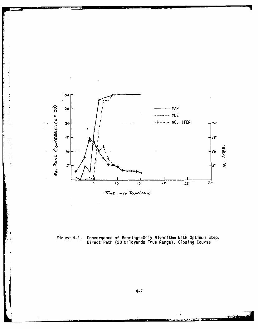
4-1 Convergence of Bearings-Only Algorithm WithOptimum-Step, Direct-Path (20 kiloyards TrueRange), Closing Course ...... ... .. ... ... 4-7
4-2a Convergence of Bearings-Only Algorithm WithOptimum-Step, Direct-Path (20 kiloyards TrueRange) Crossing-Target Course ....... .............. 4-8
4-2b Convergence of Bearings-Only Algorithm WithStep-Size Limit, Direct-Path (20 kiloyards TrueRange) Crossing-Target Course ....... .............. 4-9
4-3 Convergence of Bearings-Only Algorithm WithOptimum-Step, Direct-Path (10 kiloyards TrueRange), Crossing-Target Course ...... ............. 4-10
4-4 Convergence of Bearings-Only Algorithm WithOptimum-Step, First CZ Path, Closing-Target Course . . 4-11
4-5 Convergence of Bearings-Only Algorithm WithOptimum-Step, First CZ Path, Crossing-Target Course . . . 4-12
4-6 Convergence of Bearings-Only Algorithm WithOptimum-Step, First CZ Path, Closing-Target Course(V0 = 10 knots) ..... ..................... ..... 4-13
4-7 Convergence of Bearings-Only Algorithm With0timum-Step , First CZ Path, Crossing-Target Course# = 10 knots) .................... . 4-14
4-8 Convergence of Bearings-Only Algorithm WithOptimum-Step, Second CZ path, Closing-Target Course . . . 4-15
4-9 Convergence of Bearings-Only Algorithm WithOptimum-Step, Second CZ Path, Crossing-Target Course . . 4-16
4-10a Range Error for Bearings-Only Method WithOptimum-Step, Direct-Path, Closing-Target Course .... 4-19
4-10b Speed Error for Bearings-Only Method WithOptimum-Step, Direct-Path, Closing-Target Course .... 4-20
4-10c Course Error for Bearings-Only Method WithOptimum-Step, Direct-Path, Closing-Target Course . . . . 4-21
4-11a Range Error for Bearings-Only Method WithOptimum-Step, Direct-Path, Crossing-Target Course . . . . 4-22
iii
1-7

LIST OF ILLUSTRATIONS (Cont'd)
Figure Page
4-11b Speed Error for Bearings-Only Method WithOptimum-Step, Direct-Path, Crossing-Target Course . . . . 4-23
4-11c Course Error for Bearings-Only Method WithOptimum-Step, Direct-Path, Crossing-Target Course . . . . 4-24
4-12a Range Error for Bearings-Only Method WithOptimum-Step, First CZ Path, Crossing-Target Course . 4-25
4-12b Speed Error for Bearings-Only Method WithOptimum-Step, First CZ Path, Crossing-Target Course . . . 4-26
4-12c Course Error for Bearings-Only Method WithOptimum-Step, First CZ Path, Crossing-Target Course . . . 4-27
4-13a Range Error for Bearings-Only Method With Optimum-Step, Second CZ Path, Crossing-Target Course ...... 4-28
4-13b Speed Error for Bearings-Only Method With Optimum-Step, Second CZ Path, Crossing-Target Course ...... 4-29
4-13c Course Error for Bearings-Only Method With Optimum-Step, Second CZ Path, Crossing-Target Course ...... 4-30
4-14 Theoretical Lower Bound (Major Ellipse Axis) on Rangeand Velocity Errors for Optimum-Step Method (Direct-Path, Closing-Target Course) ... .............. .... 4-32
4-15 Theoretical Lower Bound (Major Ellipse Axis) on Rangeand Velocity Errors for Optimum-Step Method (Direct-Path, Crossing-Target Course) ....... .............. 4-33
4-16 Theoretical Lower Bound (Major Ellipse Axis) on Rangeand Velocity Errors for Optimum-Step Method (First CZPath, Closing-Target Course) ..... ... ... ... 4-34
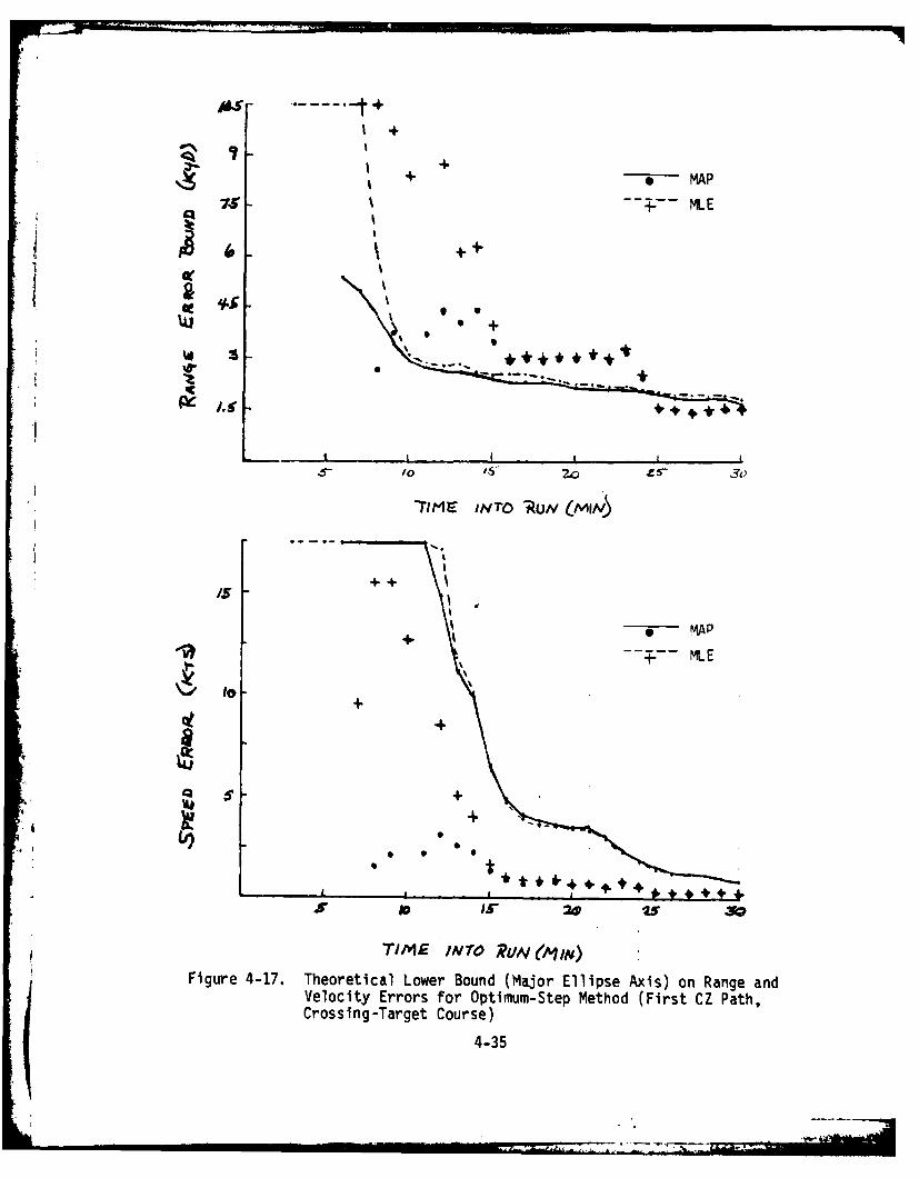
4-17 Theoretical Lower Bound (Major Ellipse Axis) on Rangeand Velocity Errors for Optimum-Step Method (First CZPath, Crossing-Target Course) ....... .............. 4-35
4-18 Theoretical Lower Bound (Major Ellipse Axis) on Rangeand Velocity Errors for Optimum-Step Method (Second CZPath, Crossing-Target Course) ....... .............. 4-36
4-19 Convergence of Bearings-Only Algorithm With Three-StateSolution (Direct-Path, Closing-Target Course) ... ...... 4-41
iv

LIST OF ILLUSTRATIONS (Cont'd)
Figure Pg
4-20 Convergence of Bearings-Only Algorithm With Three-StateSolution (Direct-Path, Crossing-Target Course) ..... 4-41
4-21 Convergence of Bearings-Only Algorithm With Three-StateSolution (Second CZ Path, Crossing-Target Course) . . .. 4-43
4-22 Accuracy (RMS Errors) of Bearings-Only Algorithm With
Three-State Solution Over Monte Carlo Repetitions(Direct-Path, Closing-Target Course) ..... .......... 4-45
4-23 Accuracy of Bearings-Only Algorithm With Three-State
Solution Over Monte Carlo Repetitions (Direct-Path,Crossing-Target Course) .... ................. ..... 4-46
4-24 Numerical Convergence of Bearing/Frequency MultisensorTMA Algorithm (Direct-Path (10 kiloyards) Closing-Target Course) ...... ... .. ... ... .... 4-50
4-25 Numerical Convergence of Bearing/Frequency MultisensorTMA Algorithm (Direct-Path (10 kiloyards) Crossing-Target Course) ...... ..................... ..... 4-51
4-26 Numerical Convergence of Bearing/Frequency MultisensorTMA Algorithm (First CZ Path, Crossing-TargetCourse) ...... ... ... ... .. ... ... .. 4-52
4-27a Range Error for Bearing/Frequency Multisensor Solution(Direct-Path, Closing-Target Course, afm = 10-2) .... 4-53
4-27b Speed Error for Bearing/Frequency Multisensor Solution(Direct-Path, Closing-Target Course, afm = 10"2) 4-54
4-27c Course Error for Bearing/Frequency Multisensor Solution(Direct-Path, Closing-Target Course, Ufm = 10-2) .... 4-55
4-28a Range Error for Bearing/Frequency Multisensor Solution(Direct-Path, Closing-Target Course, arm = 10) . . . . 4-56
4-28b Speed Error for Bearing/Frequency Multisensor Solution(Direct-Path, Closing-Target Course, ofm = 10-1) . . . . 4-57
4-28c Course Error for Bearing/Frequency Multisensor Solution(Direct-Path, Closing-Target Course, afm 10- ) . . . . 4-58
4-29a Range Error for Bearing/Frequency Multisensor Solution(Direct-Path, Crossing-Target Course, afm = 10"' ) .. .. 4-59
v

LIST OF ILLUSTRATIONS (Cont'd)
Figure Page
4-29b Speed Error for Bearing/Frequency Multisensor Solution(Direct-Path, Crossing-Target Course, afm = 10"2) . . . . 4-60
4-29c Course Error for Bearing/Frequency Multisensor Solution(Direct-Path, Crossing-Target Course, afm = 10-) .... 4-61
4-30a Range Error for Bearing/Frequency Multisensor Solution(Direct-Path, Crossing-Target Course, Of 10"-) . . . 4-62
4-30b Speed Error for Bearing/Frequency Multisensor Solution(Direct-Path, Crossing-Target Course, of 10- 3) . . 4-63
4-30c Course Error for Bearing/Frequency Multisensor Solution(Direct-Path, Crossing-Target Course, afm 10-3) .... 4-64
4-31a Range Error for Bearing/Frequency Multisensor Solution(First CZ Path, Crossing-Target Course, Gfm = 10-2) 4-65
4-31b Speed Error for Bearing/Frequency Multisensor Solution(First CZ Path, Crossing-Target Course, af = 10"2) . . . 4-66
4-31c Course Error for Bearing/Frequency Multisensor Solution(First CZ Path, Crossing-Target Course, afm = 10-2) . . . 4-67
4-32a Range Error for bearing/Frequency Multisensor Solution(First CZ Path, Crossing-Target Course, afm = 10- ) . . . 4-68
4-32b Speed Error for Bearing/Frequency Multisensor Solution(First CZ Path, Crossing-Target Course, afm = 10") . . . 4-69
4-32c Course Error for Bearing/Frequency Multisensor Solution(First CZ Path, Crossing-Target Course, afm = 10- 1) . . . 4-70
4-33 Theoretical Lower Bound on Range Error for Bearing/Frequency Multisensor Solution (Direct-Path, Closing-Target Course) ...... ..................... ..... 4-73
4 4-34 Theoretical Lower Bound on Range Error for Bearing/*1 Frequency Multisensor Solution (Direct-Path, Crossing-
Target Course) ...... ..................... ..... 4-74
4-35 Theoretical Lower Bound on Range Error for Bearing/Frequency Multisensor Solution (First CZ Path, Crossing-Target Course) ...... .................... ..... 4-75
vi

1
LIST OF TABLES
Table Page
3-1 True and Assumed Acoustic Propagation Paths andRange Values ..... .. ....................... ..... 3-1
4-1 Summary of Bearings-Only TMA Solution Statisticsat Solution Convergence Times ... ............... ..... 4-38
4-2 Solution Statistics for Direct-Path Cases With* and Without Use of Three-State Solution ............ .... 4-47
.4
vii
(Reverse Blank)

ABSTRACT
The investigation of the value of incorporating a priori information
into the TMA solution is continued in this study by computer simulations using
an asymptotically optimum estimation procedure. Two modifications to the
Maximum Likelihood and Maximum A Posteriori estimation methods for bearings-
only TMA are examined with a view toward their capability to improve numerical
convergence of the solution during early parts of the problem. The modifica-
tions are made to develop procedures which optimally use all available meas-
urements and information and to determine the true value of a priori informa-
tion incorporated into an optimum procedure. The Gauss-Newton algorithm
employed is modified such that at each solution iteration an optimum step is
taken along the calculated direction. This is accomplished by a line-search
minimization of the cost function (logarithm of the a posteriori density func-
tion). The previous procedure iterated towards a null in the linearized gra-
dient of the density function using only step-size bounds. The other modifi-
cation examined is the estimation of an observable (three-state) relative-
motion solution during the first leg which is then combined with a priori
information to obtain the full solution after a maneuver. In addition to the
study of the above modifications, multisensor MLE and MAP procedures are
developed which solve the TMA problem using bearing and frequency measure-
ments without own-ship maneuvers. Simulations are run to ascertain the impact
of range, speed, and center frequency a priori information on the numerical
convergence and solution accuracy of the multisensor algorithm.
The modified Gauss-Newton algorithm with optimum step-size calculation
improves numerical convergence for both the MLE and MAP solutions. However,
the use of a priori range estimates does further increase the probability of
convergence as well as decrease the number of iterations required, especially
during periods of poor observability. In addition, the modified procedure
does provide significant improvement in course and speed solution accuracy
during periods of poor observability when a priori range estimates are
included. The three-state relative-motion problem provides an observable
solution which consistently converges with little cost during the first TMA
ix

leg when the full solution is not observable. However, when coupled with a
priori range and speed information and post-maneuver measurements during the
second leg, it does not significantly improve numerical convergence or solu-
tion accuracy over the zero speed initialization. The numerical convergence
and solution quality of the multisensor bearing/frequency algorithm is in
*general improved by the use of range, speed, and center frequency a priori
information. This is particularly so for the cases and periods with low
observability and for the use of accurate center frequency estimates.
x -

CHAPTER I
INTRODUCTION AND OBJECTIVES
Classical Target Motion Analysis (TMA) from a time series of sensor meas-
urements involves estimating a target track which best fits the measurement
sequence according to some criteria of optimality. When the measurements are
accurate and sufficiently robust to ensure existence of a unique solution, the
problem can usually be solved in a timely manner using a variety of automatic
and/or manual techniques. In many cases of interest, measurements are not
sufficiently accurate and/or not uniquely definitive to arrive at a complete
solution. In those cases, solutions based solely on sensor measurements may
not converge or may require observation intervals that are tactically unac-
ceptable. The addition of a priori information or physical constraints may
provide tactically useful estimates when the solution is not directly observ-
able from only the measurements. This a priori information may take the form
of discrete multiple range and/or speed estimates along with some assessment
of the uncertainty in the estimates. These estimates may be obtained from
acoustic performance prediction, auxillary measurements (e.g., turn count) or
from physical constraints.
This study continues an investigation (reported in Reference 4) of the
value of incorporating a priori information into a TMA solution. Several
statistical and empirical techniques exist for solving the TMA problem which
can incorporate a priori information in some manner. Among the statistical
techniques, the Extended Kalman Filter (EKF) and Maximum Likelihood Estimate
(MLE) are most attractive from a computation viewpoint. Of the two methods,
the EKF has a much smaller computational burden but suffers from errors causedA €by "boot strap" linearization. For this reason, the MLE was selected as the
baseline TMA algorithm. This is generalized to a Maximum A Posteriori (MAP)
estimate by incorporating the probability density function (p.d.f.) of the a
priori estimates. When the a priori p.d.f.s are multi-modal (as in the
case of discrete range bands obtained from acoustic performance prediction),
the problem is segmented into parallel solutions for each mode. The parallel
solutions ar continued until incorrect alternatives can be dismissed.
1-1

The previous study (Reference 4) investigated the potential value of
incorporating external information such as range, target speed and vertical
arrival angle (D/E) into the bearings-only TMA problem. The formulation of
the TMA algorithm was based on an MLE method modified to incorporate the
external information as a priori estimates of the TMA solution with statis-
tical uncertainty. This Maximum A Posteriori Probability (MAP) estimate and
the original MLE, although not optimum in a minimum estimation error sense,
are asymptotically optimum as the data base increases without bound. The
evaluation approach taken was the direct simulation of both the MAP and MLE
algorithms using common initialization to determine the specific impact of
the a priori information on an "optimal" bearings-only TMA algorithm. The a
priori range information was treated as multiple bands of possible target
range representing the likely propagation paths. The speed information was
unimodal with various assumed uncertainty. The results of Monte Carlo simula-
tions indicated that:
1. A priori range information did not provide the expected improvement
in solution performance over a solution procedure that used the
range information as initial estimates, but it did improve the
numerical convergence of the iteration technique.
2. A priori speed information did improve both solution performance and
numerical convergence.
3. A priori range information with D/E estimates based on assumed prop-
agation path substantially improved the solution performance for
conical-angle measurement (i.e., from a line or towed array),
although more refined estimates would be beneficial.
* Since the principal benefits derived from the use of a priori information
were found to be associated with the numerical convergence properties of the
algorithm, work was continued to explore this aspect in more detail. It was
conjectured that the algorithms previously studied may not optimally use the
a priori information during the first several TMA legs where there is poor
observability. In addition, although at each numerical iteration a step size
1-2

limit was used to aid solution stability, optimum (in terms of maximum a pos-
teriori probability) steps were not used. Because of the large computation
expense incurred when numerical convergence is poor early in the TMA problem
time, it is desirable to explore ways of optimally utilizing all available
information. The objectives of this study are therefore:
1. Determine whether convergence probability and/or execution time of
the MLE and MAP algorithms are improved by the use of an optimum step
size calculation at each solution iteration.
2. Determine the value, with respect to solution convergence and accu-
racy, of utilizing procedures early in the solution to extract only
observable information.
3. Determine the value of a priori range and target speed information
optimally incorporated into the improved algorithms.
4. Address the value of a priori information in a multisensor config-
uration (e.g., bearing and frequency measurements).
The first two areas address improving solution performance during times
when measurements do not support complete, bearings-only TMA solutions.
These "improvements" were incorporated into both the MLE and MAP algorithms.
The first approach involves addition of a line search along the calculated
step direction. The optimum step size is determined at each iteration. In
the second approach, a three-state solution is implemented (in the bearings-
only TMA algorithms) during the first leg where the full solution is not
observable. After a maneuver, thf observable solution components are opti-mally combined with any a priori information and subsequent bearing measure-
ments to solve the full four-state problem. A multisensor bearing/frequency
TMA algorithm is developed and evaluated using the measurements without own-
ship maneuvers. The influence of a priori information on numerical conver-
gence time reduction and solution accuracy improvement is investigated.
1-3
P - -I

These study areas should provide benchmark results covering many of the
problem areas associated with current TMA systems. *The emphasis throughout is
placed on determining the value of external information on automatic TMA solu-
tion algorithms. As in the previous study, the computer simulations are based
on 30 Monte Carlo repetitions. The geometries simulated are typical subma-
rine maneuvering sequences. The magnitude of bearing errors used are repre-
sentative of many passive sonar systems.
'14
1-4=
I

CHAPTER I I
MATHEMATICAL ALGORITHMS AND NUMERICAL APPROACHES EMPLOYED
2.0 PROBLEM FORMULATION AND THE MAXIMUM LIKELIHOOD ESTIMATION ALGORITHM
The basic target localization/motion analysis problem is formulated, as
in the previous study, in horizontal Cartesian coordinates on a North-East
reference frame. The TMA solution, assuming a target with constant course and
speed, is completely defined by the four-dimensional state vector, x(tk), at
some time, tk, along with its state or position keeping (PK) equations.
xl(tk) target position East of origin at tk
tk x2(tk) target position North of origin at tkx3 East component of target velocity
x 4 North component of target velocity
1l0t k-tO0 0
xk) = kx(t0); *k 001 0O(2
0 0 0 1
The solution is equivalently represented (at a given time) relative to own
ship by the target range (R), course (C pe a e i
in turn, are functions of x(tk).) ped(T ndbaig(0,wih
1 2
I-I
p 4 in turnxare(functins ofxx(tk )R(tk) = LEx1(tk) - Xo1t) +x(t ) -Xos(tk))j (3)
CT = tan-'(43 )
2-1

VT= (x2 + x2) (5)
[xltk - Xs (tk)
B(tk) = tan x2(tk) X (t (6)
L 2
los(tk) is the own-ship Cartesian state vector at time tk.
The TMA solution algorithms studied are the Maximum Likelihood Estimator
(MLE) and Maximum A Posteriori (MAP) statistical estimation procedures. For
the bearings-only case with a priori information, this amounts to determining
the state estimate x which minimizes the cost function defined as the negative
logarithm of the joint a posteriori probability density function for the meas-
urement sequence 0m(tk), k=1, N. That is
vjNi 0 (7)iI x=x -
where
NJN (m(tk) " (tk)) (R(to) ITO) 2 (VT "70)o ( (tk) + 2 8)
k=1l kk
and where K0, V0 are the a priori values of range and target speed with
assumed Gaussian uncertainties OR, aV . The details of this formulation, as
well as the Gauss-Newton numerical procedure for its solution, are described
in Appendix A of the previous study report (Reference 4).
The essence of the Gauss-Newton method used previously and modified in
the present study involves a numerical iteration sequence to solve Equation(7) N
(7) and thereby achieve a local minimum of the function J . The standard
iteration algorithm obtained by expanding the gradient in a multidimensional
Taylor series about a previous or initial solution ; (tk) is:
x+l (tk) =x(tk) + a[0 < a < 1 (9)
2-2

where "a" is the scalar step size of the iteration, is the gradient vector ofN -(tk ) and^ Z is the expected value of the second partial (or Hessian)
matrix of JN at
= VxZJ N (10)
*1= E[VxL~jN] (11)
*Z is also Fisher's Information Matrix for the estimation problem, and its
inverse represents a lower bound on the covariance matrix of the solution when
] evaluated at the true solution. Equation (9) is solved by Gaussian elimination
at each iteration step until a stopping criterion, based on the normalizedmagnitude of the vector x+(tk) - Z(tk), is satisfied. The derivations forthe calculation of Z a an and of the solution x(tk) at each time step are
given, as well, in Appendix A of Reference 4.
The present study investigates two modifications to the previously used
Gauss-Newton algorithm for the MLE/MAP solution for bearings only TMA. An
optimum step size, a, is calculated at each iteration of Equation (9) along
the calculated Gauss-Newton step ([4 A]'x ). The previous procedure merely
limited the magnitude of the solution step of each Gauss-Newton iteration. In
the second approach, a three-state relative motion solution is implemented
during the first leg, where the full solution is theoretically unobservable,
of the bearings-only TMA problem. In addition, a method for bearing/frequency
multisensor TMA is developed and evaluated without own-ship maneuvers using
the same numerical approaches.4
2.1 OPTIMUM STEP SIZE CALCULATION
During the previous study, the step size for each solution iteration
(Equation 9) was limited to a physically appropriate maximum size. This was
done to facilitate convergence by not allowing the solutions to make wild
2-3

oscillations by continually overshooting the optimization surface minimum due
to poor observability (shallow minima) or linearization errors in the solu-
tion calculation. The solution step was normally selected as the Gauss-Newton
correction vector (with a=1), unless its normalized vector magnitude was
greater than some predetermined limit, in which case the correction was
reduced to meet the limit, i.e.,
1 if C2 < W2
a - 2 (12)
CJ otherwise
where
1 7
W2 + _
and where
a 2 0 0 0
0 o 0 00 1 , and a1, a2 are defined constant weights.o 0 ao 0
0 0 0 o
The locus of points which generate a constant c define a spheroid whose radius
is a1 in the x1 , x2 plane and a2 in the x3, x4 plane, and whose :enter is at
the previous solution. The surface e=1 therefore defines a small region about
the previous iteration. When c2 < 1, the iteration process is assumed to be
converged and x+(tk) is the final solution.
Although this step size limiting scheme did improve convergence, it also
was found to reduce the advantage attributable to a priori information. To
determine the extent to which the numerical procedure impacts the comparison,
2-4
I.e

it was decided to use an optimum step size calculation to determine the con-
vergence properties for solutions obtained both with and without a priori
information. The difference then should define more accurately the value of a
priori information.
The optimization of the step size parameter "a" of Equation (9) is
accomplished by a one-dimensional optimization (line search) along the Gauss-
Newton direction, based on minimizing the cost function. Therefore, the opti-
mum step size, a*, is that value of "a" between amin and amax which minimizesJN(a) along the direction on the optimization surface defined by the solution
]-i The minimum is determined by the combination of a Fibinacci search
and a quadratic fit to iN(a). The limits of search are
amin =1/
2, if > 2
a max W/e, otherwise. (13)
The Fibinacci search reduces the interval containing the minimum to
1/4 (amax - amin ) by comparing the value of JN for selected intervals. The two
end points and center value of this interval are then fitted to a quadratic
function for which the minimum is calculated by
jN(al)(al - a') + jN(a2)(a! - a) + J N(a3)(a - a)
J (al)(a 3 a2) + JN(a2 )(a1 - a3) + JN(a 3)(a2 - a,)
'.4
which is the minimum of a quadratic function fitted by Lagrangian interpola-
tion. The step size "a" to be used in the solution iteration is then
amax, if a* < amin or a* > amax
1 , if a* > 2 and amax > 1 (15)
a* , otherwise.
2-5

When convergence is achieved (el < 1), "a" is then calculated as the value mini-mizing J between amin=O and a max=2 along the solution direction.
i2.2 THREE-STATE SOLUTION
I During the initial leg of bearings-only TMA, the full solution is not
theoretically observable. Even during the first few legs, after one or two
maneuvers, observability is poor, especially for convergence-zone ranges. To
obtain useful information during the early stages of the solution when observ-
ability is poor, a three-parameter solution was calculated and used together
with the a priori information to solve the full four-parameter problem. Threepossible approaches that were considered are relative motion, constrained
range and constrained speed. The relative motion solution was selected
because it is directly applicable to both MLE and MAP methods. There is no
subset of the four Cartesian coordinates which is directly observable without
own-ship maneuvers. One can observe bearing and all derivatives of bearing at
some reference time (to). A three-state solution which defines all observable
information consists of bearing and a pair of orthogonal velocity components
normalized by range. The velocity components which most naturally relate the
derivatives of bearing are the cross range and down range velocities (i.e., RA
and 9, respectively). In this formulation, the solution vector at time t0 is
where
o k o/Ro (16)
The bearing acceleration at "to" is given by
0o -2A o (17)
2-6

Note that is not a suitable coordinate because the actual bearing timefunction is not representable by a quadratic polynomial. The three coordi-
nates presented above allow exact extrapolation to any time (t) as long as
neither ship maneuvers. The expression for bearing at any time (tk) can be
developed by simple geometry as
B(tk) = 0 + tan " ( Atk)1 + OAtk
Atk = tk -to (18)
The normalized range at tk is
P(tk = R(tk) 1 (19)
k) 7 tk) + (1 + POAtk)
Expressions for A(tk) and (tk) can be obtained by differentiating Equations
(18)and (19).
A(tk) = k/p2 (tk) (20)
(tk) = {O + (2 + 2)Atk)/P2(tk) (21)
Note that Equations (19) through (21) are not required to solve for .(tO ) but
allow one to extrapolate an estimate at "t0" to any other time. The solution
procedure for estimating the three-state solution (r(to)) is a three-state
MLE algorithm using the modified Gauss-Newton iteration procedure. The gra-
dient of O(tk) with respect to n(tO ) is readily shown to be
2-7

M1
atk cos a(tk)P(tk)
Atk sin B(tk)
jP(tk)
With B(tk), P(tk) defined in Equations (18) and (19). Thus, the iteration
equation for the relative motion solution is
i n.+l(to ) -- n.(to) + aAnL (23)
where Ant is the solution of
+ 0An =0 (24)
with
N
S(mtk) - tk)Vnt (25)ak=0
and
N= V n^ (tk)V(tk). (26)
8k=0
lea" is the optimum step size weight calculated using the procedure developed for
the full solution. The iterations continue until 2 < 1 or the maximum number
of iterations is reached.
2 JAA 2 (27)
2-8

with
01 = .010
a2 = al/T
The relative motion solution continues until own ship maneuvers. At that
time, the relative motion solution is combined with a priori information to
generate a four-state initialization solution. The relationships between therelative motion solution, target speed and target range at time tk is a func-
tion of initial range (R0).
R(tk) = R0 I(I + P0Atk) 2 + (OAtR) (28)
V2 = 060 - Vos sin(s 0 - C0 ))2 + (R0 - Vos cos( - C0 ))2 (29)
The MAP solution can be optimized directly, since minimizes the sum squared
bearing residuals for any value of R0. Then one can find the value of R0 which
minimizes the a priori terms in the cost function subject to the constraint of
Equation (29). Let
prio (R 0 " -o) + (30)Ja priori 2a' 2a
R 0 Vo (0
where I and V are a priori estimates of range and speed and 2 0 and a are
the respective variances of the estimates. Using Equation (29), V can be
explicitly defined as a function of R so the minimization is a one-
dimensional problem. When a priori speed measurements are available, the min-
imization must be performed numerically. When only range information is
available, then V=0 and aV represent a physical constraint on practical target
speeds. In that case, the optimum range estimate is
2-9
1

_ R V %i 0 cos($ - Co) - Ao sin(80o
t V
2 0~~o2 -0~o2 (31)
This procedure generates an initial solution for the second leg of the TMA
problem, which is based on solving for the information observable from the
bearing data using a modified Gauss-Newton MLE algorithm, which is then opti-
mally combined with a priori information to generate a complete solution.
This procedure should provide the optimum solution available from the first
leg if the a priori model is correct. Since the relative motion solution is
independent of range, it is common to all propagation path assumptions. If
the combination of relative solutions with a priori range is performed for all
path assumptions, it may be possible to determine the correct path by examin-
ing the speed estimates given by Equation (29). This would depend on geometry
and bearing accuracy. For example, a high bearing wate, 'Irtct-path geometry
would be distinguishable from a convergence zone but a closing geometry may
not resolve the correct path.
2-10 ~1~.*

I
2.3 BEARING AND FREQUENCY MULTISENSOR TMA
For bearings-only problems, own ship must maneuver to obtain a full TMA
solution. When additional measurements are available, such as range rate
(from Doppler analysis of frequency measurements) or bearings from another
array, it may not be necessary to maneuver. Convergence without maneuvers,
however, may be too slow for tactical considerations, and thus the use of a
priori information can potentially be of value in reducing solution converg-
ence time. This aspect of the problem can be investigated by TMA simulations
using the MLE and MAP algorithms modified to accept multisensor data. Note
that maneuvers were not precluded for this case but were not considered
because the problem would be similar to the bearings-only problem. Also, they
did not provide additional insight to the value of a priori information.
An algorithm for the solution of a bearing/frequency multisensor TMA is
developed using the MLE/MAP approach. The problem formulation is the same as
that for the bearings-only case, i.e., a four-state horizontal solution in
Cartesian coordinates, except that frequency measurements are used along with
bearings, and the test runs are made without own-ship maneuvers. There are
five solution parameters since the base frequency (fo) (without Doppler
shift) must be estimated. A procedure is developed in the Appendix to opti-
mize f0 as an explicit function of the estimated range rate (a function of the
state solution), the frequency measurements and the a priori estimate of f0The value of incorporating a priori knowledge of f0 is therefore evaluated
along with that of range and speed.
The development of the computations for the bearing/frequency MLE (or
more specifically MAP) approach with a priori knowledge of the base frequency
is given in the Appendix. The MAP algorithm using additional a priori infor-
mation (range and speed) is formed by incorporating into the a priori proba-
bility density function (p.d.f.), developed in the Appendix, the appropriate a
priori p.d.f.s. This results, as in the bearings-only case, in additive terms
in the log likelihood ratio for the state vector:
i R = + LR + 1 - RO'2 + V7 o V0)2 (32)
2-111

where JLR is the log likelihood ratio (cost function) from Equation (20) of
the Appendix.
The first and second gradients of JLR with respect to the reference state
vector x(tO) are required for the Gauss-Newton solution procedure. The calcu-
lations for the gradients of JLR are derived in the Appendix. The gradient
calculations for the range and velocity a priori terms are the same as in the
bearings-only algorithm except for the second gradient of the a priori veloc-
ity term. When speed is unknown a priori but is bounded by physical con-
*straints, the speed estimate is zero and the sigma represents an average speed
(or one-half of the maximum speed). The a priori velocity term in Equation
(32) would be
(AV2(to) x2(to) + x2(to )
LO V0 0
The second gradient of J is then1o
T 0
I°v ] o (34)[2a^aV
where I is the 2x2 identity matrix. This expression for the second gradient
is unfortunately not consistent with that used in the bearings-only cases.
The expression presented in the previous study was developed for use with a
priori speed estimates and does not collapse to the correct expression when a
priori speed is not available. Fortunately, the speed term does not affect
the solution in that case, when only bearing inputs are observed. For bearing
and frequency observations, the frequency measurements are related to veloc-
ity and it was found that the velocity components of the * matrix formed a
singular matrix when the incorrect second gradient was used. This did not
occur with the bearings-only inputs. During investigation of this problem, it
became apparent that MLE should be formulated (when no a priori information is
available) by incorporating range and speed bounds in the cost function as I2-12 I

R2(tO) V2(to )
LE "MLE (35)+a _2max
Where Rmax and Vmax are chosen to bound the expected range and speed. This
form would lead to a * matrix of the form
1
max= MLE + (36)i o 1
0 V,_max
This would have the properties of the Marquardt Gauss-Newton algorithm using aphysical constraint. This procedure was not evaluated but it will guarantee apositive definite 4# matrix and will not bias the solution if Rmax and Vmax are
chosen correctly.
2-13
I-l

CHAPTER III
SIMULATED TMA SCENARIOS
3.0 OPERATIONAL SCENARIOS
iThe operational scenarios simulated for the present study are basically
the same as those described in the previous report (Reference 4). Own ship to
target ranges from 10 to 109 kiloyards were modeled covering direct, first and
seconid convergence zone (CZ) acoustic propagation paths. The acoustic propa-
gation properties assumed are realistic, yet general enough to represent many
different oceanographic conditions. The target-ship courses used, which
remained constant over a given run, were 146 degrees and 256 degrees. These
present an initial broadside (crossing) and closing aspect, respectively.
Table 3-1 summarizes the propagation paths and initial true target ranges as
well as the initial range estimates and standard deviations used in the TMA
computer simulations.
Table 3-1. True and Assumed Acoustic Propagation Paths and Range Values
TARGET COURSE PROPAGATION TRUE PATH TRUE TARGET ASSUMED RANGE URRANGE RANGE 0(deg) PATH (kyd) (kyd) (kyd) (kyd)
Direct 0-30 10, 20 15 7.5256 1st CZ 45-55 54 45 4.5
(closing) 2nd CZ 90-110 109 90 9
Direct 0-30 10, 20 15 7.5146 1st CZ 45-55 46 55 5.5
~(crossing) 2nd CZ 90-110 91 110 11
Initial true bearing was 56 degrees for all runs. Own ship had an initial
bearing of 0 degrees and maneuvers consisting of standard 60-degree lead/
60-degree lag with leg times of 5 minutes duration and turn rate of 2 degrees
per second. Both own ship and target maintained a constant speed of 10 knots.
3-1

3.1 SIMULATIONS
Simulations were run in three phases. These were the bearings-only case
with optimum step size calculation, the bearings-only case with a three-state
relative motion solution during the initial TMA leg, and the bearing/
frequency multisensor case with no own-ship maneuvers. Each simulation of all
three phases was run with 30 Monte Carlo repetitions, and with run times of
15 minutes for direct-path true range and 30 minutes for the CZ true range
cases. Measurements of bearing or bearing and frequency were input to the TMA
problem every 20 seconds, and solutions calculated by the MLE or MAP algorithm
every minute. Bearing measurement error for the 20-second averages was
unbiased with a8 = 0.2 degrees for all but a few of the bearings-only runs which
had a8 = 0.5 degrees. Frequency measurements were expressed as normalized Doppler
shifted values of the true center frequency (f0 = 1) using the true simulated
range rate values. The frequency measurement error standard deviations (ofm)
were 10"3 and 10-4 , again normalized by the center frequency. The noise com-
ponent of each measurement time series was simulated from a Gaussian pseudo-
random number generator, with an independent sequence used for each Monte
Carlo repetition.
3.2 A PRIoRZ ESTIMATES
Initial values for range, speed and center frequency with uncertainties
were defined for use as solution initialization and a priori estimates. The a
priori range values and uncertainties assumed in the various runs are listed
in Table 3-1. Initialization for the position coordinates of the solution are
calculated from these assumed range values and the first bearing measurement.
The velocity terms are initialized as zero since no a priori course informa-
tion is assumed. The assumed mean center frequency (T0) is taken as the true
value for the a priori runs and as the first frequency measurement when no a
priori knowledge is assumed. A priori values for velocity and center fre-
quency with their uncertainties that were used in the simulations were:
3-2

Velocity: case 1) V0 = 0; =v 15
2) V0 = 10; oV0 =4
3) V0 = 10; oVO = 2
Center Frequency: case 1) To = 1; Ofo = 10-,
2) To = 1; afo = 1-
3-3

CHAPTER IV
DISCUSSION OF SIMULATION RESULTS
4.0 OVERVIEW OF RESULTS PRESENTED
The TMA scenarios described in the previous chapter were simulated with
the overall objective of evaluating the importance of external information in
achieving accurate and timely target motion solutions. The MLE and MAP pro-
cedures using the numerical algorithms derived in Chapter II were chosen as
the methods to best demonstrate the potential utility of such information.
The improvement attained by incorporating a priori statistical estimates of
range, speed and center frequency is shown by comparing the solution results
of Monte Carlo simulations using the MAP estimation procedure to those using
the MLE. The MLE procedure uses the external information merely for initial-
ization of the iterative numerical solution and not as part of the estimation.
The contribution of the a priori information to the bearings-only and
bearing/frequency solutions is measured by the improved accuracy and reduced
convergence time achieved. The measures of solution accuracy are obtained by
calculating the mean and standard deviation of errors over the Monte Carlo
repetitions. Measure of potential solution quality from the information
available is obtained from the error bounds as calculated from the eigen-
values of the inverse Fisher's information matrix for the estimation problem.
These error-bound estimates are the Cramer-Rao lower bounds on solution
accuracy when evaluated at the exact solution. Solution convergence is
defined as the reduction of the error bounds below some defined level.
A Improvement in numerical convergence is measured by the reduction of computa-
tional burden of the algorithm as represented by the number of Gauss-Newton
iterations required for each solution. Numerical convergence probability is
determined from the number of Monte Carlo repetitions at each solution time
which do converge, defined by satisfying the stopping criteria within
21 iterations.
4-1
I

The results presented in this chapter are separated into three sections,
based on the numerical procedure being evaluated. The first two sections
present the results for evaluation of modifications to the bearings-only
MLE/MAP algorithm which was developed in the previous study. Since the value
of a priori information may be highly dependent on the particular numerical
methods employed, improvements to the algorithms to most efficiently use all
available information were studied. The effect of the numerical modifica-
tions on solution accuracy and convergence is, therefore, evaluated along
with and within the context of the incorporation of a priori information. The
numerical modifications studied are, respectively, calculation of an optimum
step size at each Gauss-Newton iteration by a cost function line search and
solution of a three-state, relative-motion problem during the first TMA leg.
The third section presents results of simulations which were run to evaluate
the incorporation of a priori information into a multisensor (bearing and fre-
quency) MLE algorithm without own-ship maneuvers.
4.1 BEARINGS-ONLY MLE USING OPTIMUM STEP-SIZE CALCULATION
The results of the previous study's simulations indicated that the prin-
cipal advantage of a priori range information is related to the numerical con-
vergence of the solution procedure rather than its ultimate accuracy. Modifi-
cation of the Gauss-Newton algorithm to improve numerical convergence without
a priori information may therefore affect the observed value of incorporating
such information into the algorithm. The Gauss-Newton algorithm used previ-
ously was modified, as described in Section 2.1, to optimize the step size
taken at each iteration in the calculated direction with respect to the actual
cost function. Previously, the step taken was the full solution step of the
linearized optimization, subject only to a magnitude limit, without regard to
the change in the actual cost function. It was conjectured that optimizing
the step size would reduce the numerical convergence time of the algorithms,
as well as improve the solution quality early in the problem. This, however,
may in turn either negate any improvement previously provided by incorpora-
tion of a priori information or may enhance such improvement by more optimally
using the available information.
4-2

The results of Monte Carlo simulation runs are presented using the modi-
fied Gauss-Newton procedure. The TMA scenarios simulated are as described in
Chapter III and are the same as in the previous study. Both closing and
crossing target aspects are analyzed with own ship executing maneuvers. For
the direct-path case (range = 20 kiloyards) runs were made with assumed a
priori ranges in the direct, first CZ and second CZ propagation paths. CZ
runs have the same true and assumed paths. In addition, direct-path runs were
made with true range of 10 kiloyards and assumed range in the direct path.
One direct-path run was also made with bearing error standard deviation of
0.5 degree (all others were with 0 = 0.2 degree). Additional first CZ runs
were made including speed a priori information with estimate equal to the true
target speed (10 knots) and standard deviations of 4 and 2 knots.
4.1.1 Preliminary Study of the Step-Size Optimization
Before considering the results of the Monte Carlo simulation runs, a pre-
liminary analysis of cost function behavior versus step size and of its mini-
mization is carried out. In addition, the computational cost for the inclu-
sion of the step-size optimization procedure in the MLE algorithms is esti-
mated. This estimate may be used to weigh any benefits from the procedure
against its added cost.
The modified Gauss-Newton method solves the non-linear optimization
problem with an iterative series of linearized solutions, calculated until
satisfying a convergence criterion. The change in the solution at each itera-
tion may be expressed as the vector difference between the previous solution
and the present one. This solution update is given at each iteration by:
A A
Ax = ! = -CWI VxJ (1)
where Ao is the solution vector calculated by the Gauss-Newton procedure as
described in Section 2.1, and is the magnitude of the step actually takenA
from the previous solution in the A direction. Under the assumptions used
4-3

to ensure convergence of the modified Gauss-Newton procedure, the change in
the cost function, AJ, may be modeled approximately as a quadratic function
of the solution change vector using terms of the multidimensional Taylor
series expansion
&] =VT *1 ^T T(2
This may then be expressed as a function of the step size, using Equation (1):
I AtJ :-aV~j@ixVxJO -: VxJI-1VxVTJ*'JIVxJ
61= vT *Ix + a2 V T J*-1Vx F-O _' x x
SAj ^T _ _ _+ Tr T
Sis (T a + L r) (3)
whereA^T T
r = (4)
for ae(O, 11.
The step-size limiting procedure used in the previous study set a to a value
between the limits of 0 and 1 based on a maximum allowable magnitude for Ax
defined by reasonable physical constraints. The modified procedure deter-mines a by a numerical line search minimization of J(x,a) at each iteration.
This procedure may be modeled analytically by minimizing Equation (3) with
respect to a. This yields
1/r;r>1
n ; otherwise (5)
4-4
, a1

when subject to the constraint ae[0,1]. The actual procedure used, however,
constrains the step size ocz[min, %max ] where amin > 0 is the minimum step
taken and %lax < 2 is the step-size limit, whose values are determined as
described in Section 2.1.
In preliminary runs of the algorithm in both the original and modified
form, the behavior of J(a) was observed at several intervals along the calcu-
lated solution direction. These observations showed that at numerous itera-tions the minimum occurred at a's near to or less than zero. This was most
prevalent before complete solution observability but also occurred later in
the problem. Since the quadratic model above (Equations (2) through (4)) does
not predict optimum solutions for a < 0, this result reflects a domination by
higher order, (unmodeled) terms indicating that J(a) is not approximately
quadratic at the trial solution. In fact, if the "optimum" step is taken, the
solution collapses to the previous solution. The calculated Gauss-Newtonsolution is therefore not always consistent with minimization of the cost
function. To solve this problem, it was found that taking a limited step in
the Gauss-Newton solution direction allowed eventual convergence even though
the cost function was not minimized. This observation clearly shows the value
of step-size limiting for solution stabilization. However, oscillation
between poor solutions may still occur preventing early convergence. Step-
size optimization should help convergence further by directing the Gauss-
Newton solution towards consistency with the cost function minimum (except
under the noted singular conditions). Minimization of the cost function in
the vicinity of the converged solution may also improve solution accuracy,
especially early in the problem when solution updates are large.
Inclusion of a priori information appears to stabilize the Gauss-Newton
solution such that wild oscillation would not occur even without step-size
limiting. This is clearly seen in the cost function values at and in the
direction of the calculated solution. Optimization of step size would there-
fore not be expected to improve convergence of the MAP algorithm to the same
extent that it would for the MLE. However, solution accuracy may be improved
during the problem time before solution convergence in the same manner as
without a priori information.
4-5
I

Estimates for the computation cost of the step-size optimization are
made by running simulations for various problem times without the Monte Carlo
statistics calculations. Cost estimates are in the form of computer proces-
sing (CPU) time. Although such estimates are approximate and the true cost
may vary for different data sets and TMA conditions, as well as for different
line search algorithms and codings, they may be helpful for rough comparisons
between the added calculations' cost and any measured benefit. These test
runs produced estimates for the added cost of the step-size calculations to
the Gauss-Newton algorithm of 15 to 25 percent. In addition, these direct
* propagation path simulations indicated that the savings in computation time
from better convergence of the modified algorithm did not make up for the
added cost of the procedure. However, an enhanced quality of early solutions
may be gained.
4.1.2 Numerical Convergence Properties of the Modified Gauss-Newton
Algorithm
The numerical convergence properties of the modified bearings-only algo-
rithm are shown in Figures 4-1 through 4-9 for all TM geometries simulated.
The number of Monte Carlo repetitions, out of the 30 run, which meet the
numerical convergence criterion are plotted for each calculation time along
with the average number of Gauss-Newton iterations required for convergence.
These measurements represent, respectively, the probability of obtaining a
converged solution at each problem time and the computational requirement for
convergence. In each figure, the MLE and MAP solution results are presented
for cases assuming the correct propagation path and using a measurement
bearing-error standard deviation of 0.2 degree. Results are presented for
direct, first CZ and second CZ propagation path cases without use of a priori
speed estimates. For the first CZ cases, results are also given for the MAP
solution with a priori speed estimates with standard deviation of 4 and
2 knots (Figures 4-6 and 4-7). Direct-path results are given for cases with
initial true ranges of 20 and 10 kiloyards. The results from the use of the
step-size limiting algorithm are also included for the direct-path, crossing-
course case (Figure 4-2b). Comparison of the two procedures for the other
4-6 I
I+/
". " M A P
-- - - MLE
-- --- - NO. ITER -o
4,
o , 0 1" 2-
++.Figure 4-1 Convergence of Bearings-Only Algorithm With Optimum Step,+ Direct Path (20 kiloyards True Range), Closing Course
4-7

I
4 w . . ... ... . .
.. ... MAP
- - MLE
.... .. ~ .............
-,0 .. .... 2 9 ... .... ...7i'
Figure 4-2a. C -o-n- NO. ITER ..... Step,
-. 4-4
Figure 4-2a. Convergence of Bearings-Only Algorithm With Optimum Step,Direct Path (20 kiloyards True Range), Crossing-TargetCourse
4-8
"1*L [~

C IG
0
U' mLE,l -- +- NO. ITER 20
10 Is aI
T I ro Pt (CU4-
I $$
I I I I
£" 1o 15" ;a c
Figure 4-2b. Convergence of Bearings-Only Algorithm With Step-Size Limit,Direct Path (20 kiloyards True Range) Crossing-Target Course
4-9

30
_ MAP
- MLE-.-- I-NO. ITER 0
101 20
_rN 14N tf
Direct Path (10 kiloyards True Range), Crossing-TargetCourse
4-10
F. W O I

ft.' _ MAP
O I----------MLE
' 4-+ NO. ITER .
-rms5V/V
Fure44 ovrec fBaig-nyAgrtmWt piu tp
Fis CZPtCoig-agtCus
I4-1

MAP
''-++-NO. ITER_
. .. . . .. .
* Figure 4-5. Convergence of Bearings-Only Algorithm With Optimum Step,First CZ Path, Crossing-Target Course
4-12

av 0 2 knots
ZD~ -- -= 4knots Z
eo*.eaV = 15 knots
0 4-+-4- NO. ITER
+f
7-Imi AWTV R&W CA e)
Figure 4-6. Convergence of Bearings-only Algorithm With Optimum Step,tA First CZ Path, Closing-Target Course (V =10 knots)
4-13

I ~~~~~~ =A F2tC ahi~0 knots
Crossng-Trget ours ( 0 15 knots
4- -+-N.14E
" ~/ "-3 0TI-" "- TII
T7o~ *M b AfM
Fiue47 ovrec fBaig-nyAgrtmWt piu tp
Fis ZPtCosn-agtCus i=0kos
4-1
po

a-t,-MAP--- --MLE
4++++NO. ITER
V) ..
Figure 4-8. Convergence of Bearings-Only Algorithm With Optimum Step,Second CZ Path, Closing-Target Course
4-15
I' /iI

M~AP . .-
---MLE * w
NO ITR V
.79
Figure 4-9. Convergence of Bearings-Only Algorithm With Optimum Step,Second CZ Path, Crossing-Target Course
4-16

geometries may be made using the results given in Section 3.1.3 of the previ-
ous report (Reference 4).
The results of numerical convergence frequency versus problem time for
the Monte Carlo repetitions shown here generally agree with those of the pre-
vious study. They clearly demonstrate the benefit derived from incorporation
of a priori range and speed inputs towards increasing the probability of
numerical convergence. This is particularly noted for the difficult geome-
tries and during the early parts of the problem. For the direct-path cases,
the MAP algorithm frequently converges on the first leg while the MLE almost
never does. Since the complete solution is not observable, this behavior is
expected and does not represent a significant advantage to the MAP solution.
After the first leg, convergence is virtually equivalent for both cases. The
MAP solution does converge more frequently during the maneuver. The first and
second CZ cases with the closing target course geometry show a marked increase
in convergence probability due to the use of the MAP algorithm. This is seen
during the second through fourth TMA legs of the first CZ case and throughout
the entire run for the second CZ case.
The use of the optimum step-size calculation appears-to increase the
probability of convergence for both the MAP and MLE algorithms over the step-
limiting method. The measured improvement in convergence due to a priori
information use therefore remains approximately the same.
The previous study concluded that the major computer burden of the algo-
rithms is associated with the unsuccessful search for a (numerically) con-
verged solution, and therefore the MAP solutions require fewer computations
than the MLE simply because more solutions converge within the maximum itera-tion limit. This conclusion is only partially substantiated by the results
shown here for the algorithms using optimum step size. The average number of
iterations required for convergence versus problem time is plotted for all
converged Monte Carlo repetitions. These numbers therefore exclude any com-
puter cost due to a solution failing to converge with the alloted Gauss-Newton
repetitions. In general, the results for the crossing-course geometries show
4-17
- . . - . . . .,-- rn, *- - -Y

little difference in average iteration number between the MAP and MLE solu-
tions. However, those for the closing course, a more difficult TMA geometry,
show the MAP to converge on average with fewer iterations. This is particu-
larly the case during the early legs and with the CZ cases.
4.1.3 Solution Behavior for Correct-Path Hypotheses
The earlier results from MAP and MLE algorithms, not employing step-size
optimization, indicated that the major value of a priori range information was
improved numerical convergence of the solution rather than improvement of the
intermediary and ultimate solutions. Therefore, it was observed that
although comparison was made to MLE algorithms which benefit from good initial-
ization using the a priori range estimates, the value of using correct a
priori range information in a MAP algorithm was disappointing. Little gain in
solution accuracy and solution convergence time was measured.
Figures 4-10 through 4-13 show the solution errors as a function of prob-
lem time for simulations employing step-size optimization and using the cor-
rect propagation path assumptions for solution initialization and a priori
estimates. Parts a, b and c of each figure give the range, speed and course
errors, respectively, averaged over all numerically converged Monte Carlo
repetitions. The solid and dashed lines represent the root mean square errors
of the MAP and MLE solutions respectively, and the symbols (e and +) represent
the mean errors at each problem time. Results are presented for the direct-
path (20-kiloyard range) case with closing course geometry and for all three
propagation paths (direct, first CZ and second CZ) with crossing course geom-
etry. The CZ results for the difficult closing geometry are basically very
poor and are not presented. The direct-path results show only a very small
(if any) decrease in range and course RMS error due to a priori information
use and no difference in solution convergence time. The speed RMS error for
the MAP algorithm is considerably lower during the second TMA leg. A very
small negative bias in the MAP speed error is still noted at the later legs
after convergence for the closing-course case. The results for the first and
second CZ cases with crossing course show a more pronounced decrease due to
4-18
I

- - MAP RMS ERRORMLE RMS ERROR
b I. S MAP MEAN ERROR+ MLE MEAN ERROR
0'
Ad +
-rm /t47 R/T UN (MIN)
Figure 4-10a. Range Error for Bearings-Only Method With Optimum-Step,Direct-Path, Closing -Target Course

'U
-MAP RMS ERROR
- MLE RMS ERROR
* MAP MEAN ERROR
+ MLE MEAN ERROR
s-
+ +
o+
0 + +
1 l
402* 10 Ia as-, ,
'r IM INT RLoN "I Ao
Figure 4-l0b. Speed Error for Bearings-Only Method With Optimum-Step,Direct-Path, Closing-Target Course
4-20 .
1I
-2" -9-

MAP RMS ERRORMLE RMS ERROR
o MAP MEAN ERRORMLE MEAN ERROR
II
300• ! +
3o o, * ,
i+
.+ +
*0t44
0+i~-0
U
-60
'1I , I I I A/)
Figure 4-10c. Course Error for Bearings-Only Method With Optimum-Step,Direct-Path, Closing-Target Course
4-21

MAP RMS ERROR
MLE RMS ERRORMPMEAN ERROR
+ MLE MEAN ERROR
-3
I4.
to Is,
TIMU INTO RUN LrtlN)
Figure 4-11a. Range Error for Bearings-Only Method With Optimum-Step,Direct-Path, Crossing-Target Course
4-22

I I I I
j MAP RMS ERROR
"" MLE RMS ERROR
* MAP MEAN ERROR
+ MLE MEAN ERROR
Fiur 4-b Spe ro o ernsOl ehdWt piu-tp
a I ----.
-42
_ I I I I IS I. 15 i.F 30
Figure 4-l1b. Speed Error for Bearings-Only Method With Optimum-Step,Direct-Path, Crossing-Target Course
4-23

- MAP RMS ERROR
MLE RMS ERROR
* MAP MEAN ERROR
+ MLE MEAN ERROR
0O- . .
+ 400
0 °
-4-0
I I I.~**j ... .. .. I I I
-TVM E iNTO IV)N (l'lIIN )
Figure 4-11c. Course Error for Bearings-Only Method With Optimum-Step,Direct-Path, Crossing -Target Course
4-24

\ ? I
MAP RMS ERROR
.MLE RMS ERRORj * MAP MEAN ERROR
S"+ MLE MEAN ERROR
400
I S 0
1~~ o ** *- S-F-
I
4-25. 4
f • - I , I 1 I10'8"I I,,S 2o 25 So
, "li'ME iNTO RUN LtvlIw)
Figure 4-12a. Range Error for Bearings-Only Method With Optimum-Step,First CZ Path, Crossing-Target Course
4-25

+ML " I 1
I 4"
+ MAP RMS ERRORI /I MLE RMS ERROR
0 MAP MEAN ERROR
+ MLE MEAN ERROR
+ +
-I4
-VI
I11I I
,. Ioii 20 Us" 30
T)~'W INTO RLW (IN)
Figure 4-12b. Speed Error for Bearings-Only Method With Optimum-Step,First CZ Path, Crossing-Target Course
4-26

IL
MAP RMS ERROR
.... - MLE RMS ERROR* MAP MEAN ERROR
-. ,+ MLE MEAN ERRORA
+ +
+. + +
4 -34-
I 1I I003
-riM Cr I/TO AWu/ MIA/)
Figure 4-12c. Course Error for Bearings-Only Method With Optimum-Step,First CZ Path, Crossing-Target Course
4-27
- i "
Fiue41 Cus ro fo Berns-nyMehdWthOtmu-tp

MA RM ERRO
qL M RO
S ____MAP MSA ERROR
+ MLE MEAN ERROR
a +
-3 + +. +
. + 4
-,+ +
14. 20 dozs
71ME INTO RVN (MIN
Figure 4-13a. Range Error for Bearings-Only Method With Optimum-Step,Second CZ Path, Crossing-Target Course
4-28

IMAP RMS ERROR
MLE RMS ERROR
* MAP MEAN ERROR
+ MIE MEAN ERROR
0 0
+-4.. +2.-.
116.
(A
33
4-29

'. MAP RMS ERROR
\ MLE RMS ERROR
- ' MAP MEAN ERROR+ V/
+ MLE MEAN ERROR
| . -" •4..
o I 4. +
++
5'1 10 15J..3 3
-Time INTO R AI ( I /N)
Figure 4-13c. Course Error for Bearings-Only Method With Optimum-Step,Second CZ path, Crossing-Target Course
4-30

the MAP algorithm in range, speed and course RMS error in the early legs.
This difference disappears at or before solution convergence. The range mean
errors for both the MAP and MLE methods are biased even at later problem
times, however in opposite directions.
The above results, therefore, do show that for an algorithm using an
optimum step-size calculation the incorporation of a prior! information does
yield, for some geometries, significant improvement in early leg solution
accuracy. However, ultimate solution convergence and ultimate solution accu-
racy are not enhanced.
4.1.4 Error Lower Bounds and Solution Convergence
In the operational environment, values for the TMA solution errors are
not known. It is important, therefore, to estimate solution performance and
convergence status. An estimate for Fisher's information matrix (* matrix) is
calculated as part of the MLE and MAP solution procedure. The inverse of this
matrix, when calculated using the true solution, is the Cramer-Rao lower bound
on the solution error covariance. Therefore, this can be used even when cal-
culated at solution estimates, to indicate sensitivity of the solution to
additional measurements and to place a relative estimate on the solution qual-
ity theoretically obtainable. The covariance lower bound matrix is converted
to independent scalar parameters by partitioning the inverse matrix (*-1) into
2X2 position and velocity submatrices and computing their eigenvalues. The
square root of the larger elgenvalue for each set represents the major axes of
the position error ellipse and of the total velocity error ellipse. These are
theoretical lower bounds on range error and total velocity vector error,
respectively.
The major axes for the range and velocity error bounds are plotted in
Figures 4-14 through 4-18 for the direct, first CZ and second CZ path cases.
The crossing geometry results are included for all three path cases, whereas
the closing course results are for only the direct and first CZ cases. The
error bounds for both the MAP and MLE solutions are included (solid and dashed
4-31

o . MAP
M fLE
SI R,5* m
.is
o * MAP
2:
-K E10
+
Io 12v as so
-1ME INTO RUN CMlIN)Figure 4-14. Theoretical Lower Bound (Major Ellipse Axis) on Range and
Velocity Errors for Optimum-Step Method (Direct-Path,Closing -Target Course)
4-32
Ki

. . .. rMAPL-- -- MLE
ICE
(P
3[
I 9., t t
I M I I
.tITIr~i INTO ?.)IpLt iIlN)
,11I
'I,
I • MAP
.5 -i- - ZE
TIMG No RuN CmiN)Figure 4-15. Theoretical Lower Bound (Major Ellipse Axis) on Range and
Velocity Errors for Optimum-Step Method (Direct-Path,Crossing -Target Course)
4-33

%,/
7.5- ~.- LE
6+
I
03
TIME 1A1T0 R"N (,'Ii
A6v+
~4-34
+
+ .- MAP75 - -- LE
(0 + ++
M P
t I , , I
+4T,V (Al MAP
4-3
\.' Io 4
Q 5
II5"
Tit'E iNTo RUN (bi I)
Figure 4-17. Theoretical Lower Bound (Major Ellipse Axis) on Range andVelocity Errors for Optimum-Step Method (First CZ Path,Crossing-Target Course)
4-35

7~
q + +
4 ++ITS -+ + ",
++
1+ +W MAP
'II a -I- VLE
.!.
- , I I I I I
T/1ME INTO RUNv CrMll)
3,,
L I +
.4.4- + + +4
to i.- 30
TIMEw ),TO RN( N
Figure 4-18. Theoretical Lower Bound (Major Ellipse Axis) on Range andVelocity Errors for Optimum-Step Method (Second CZ Path,Crossing -Target Course)
4-36

lines) along with the Monte Carlo standard deviations for solution times with
a high (>67 percent) probability of convergence (e and +). The observations
made from the error-bound plots are essentially the same as those for the
algorithm without step optimization presented in the previous report. The
error lower bounds are lower for the MAP solutions than those for the MLE,
particularly during the early legs. The measured increase in solution accu-
racy for the MAP algorithm, noted in the previous section but not in the pre-
vious report, is therefore due to better utilization of the a priori informa-
tion by the algorithm modified for step optimization rather than due to any
enhancement in the best solution theoretically achievable. Consequently, the
solution convergence behavior for both the MAP and MLE remains unchanged by
the modified algorithm.
Table 4-1 presents a summary of the numerical and solution characteris-
tics for the modified bearings-only MLE and MAP algorithms. Results for simu-
lations of each geometry/path hypothesis are included. Included in the sum-
mary for each simulation are averages of the numerical convergence measure-
ments, estimate for solution convergence time and the RMS error characteris-
tics of the solution at the determined convergence time. The criterion for
solution convergence was defined as in the previous study as the time at which
the velocity major axis error bound reaches 1 knot (10 percent of actual
velocity magnitude). This is somewhat arbitrary but is sufficient for compar-
ison purposes. The range error bound and the Monte Carlo solution error sta-
tistics may be used to confirm the solution convergence time and the converged
solution's validity. The values presented in Table 4-1 may be compared with
those in Table 3-1 of the previous study for the algorithms without step opti-
mization.
Using the statistics presented in the table comparison between the MAP
and MLE algorithm may be made and thus the value of a priori information may
be estimated. The number of converged Monte Carlo repetitions and the number
of Gauss-Newton iterations per repetition averaged over all solutions of the
runs are indicative of the relative computation costs of the runs. The solu-
tion convergence time and the RMS errors at that time give a relative indica-
* tion of the solution's timeliness and quality. In general, the use of a priori
4-37
.-

9 - C Ili C9 G! En n 19 N8 C-4
I.- U~~I- __ _ _ _ _
000,. - (n 0 m N NU O a. co2a) - --
Q- N. a, 4nm- n
z.
0P m
.4J.
.4-)
v'R 9 I a-! - 0 o 4 c !9
co %D04m m m c oI
w 0 o -w c,- - - - - - - - - n En
'a I-
w0 0 9 000 m m0 -wWW mW Go 101-s c mb
c; I~ - N
- 9
4- Q j c0 09W Nz 0 N cn E nE nE n
) VN O -
~. N 90O En0% UN 9 0 U En 0U)
09E 0 n E N En - N u n .
Lc~ 0%0 ND ND N Q0 gN U NU O N U
Uj -A --- NA MA "Al T90A M :
>9l
o~~~ ~ ~ ~ -090 ON EnOc0 U N-U e E 0 00%wo 9' n 0 n 0 W N 0 0W 0W 0
14 <-- c34S 'A
o19 Qj -. 9-4
3S~~~nOO9- AS.3WO 3w~0I.. N ONSO N 09 0 9 90 9C 0W
4-3

information in the algorithm with step optimization decreases the whole run
average computation cost of obtaining numerically-converged solutions for
both closing and crossing-course geometries and for all propagation paths.
The CZ cases for the crossing-course geometry, however, are only slightly
affected. Solution convergence time appears to be unaffected by the use of a
priori estimates. However, in the simulations used here, the defined converg-
ence criterion often is not reached by the end of the problem time. Solution
accuracy, as defined by RMS error averages across Monte Carlo repetitions,
appears to be inconsistently improved by using the MAP algorithm. The
crossing-course geometries show little difference in RMS range, speed and
* course errors at the convergence times between the MAP and MLE solutions. The
direct and second CZ cases with closing-course geometry have slightly
decreased range and speed RMS error from the use of correct a priori range
information, and the first CZ case has decreased speed RMS error from a priori
speed estimates. It should be noted that the error estimates compared are
those at the solution convergence time only and that the results of Sec-
tion 4.1.2 should be used for further comparisons. In addition, the error
estimates based on the Monte Carlo repetition averages have limited useful-
ness since 30 repetitions are probably not sufficient for accurate
estimation.
4.2 BEARINGS-ONLY MLE WITH THREE-STATE, RELATIVE-MOTION SOLUTION
The calculation of a three-state solution to the bearings-only TMA prob-
lem was incorporated into the MLE/MAP algorithms in order to optimally utilize
the available data when the full solution is not theoretically observable.
The results presented in this section are from simulations using the modified
Gauss-Newton algorithm (with step optimization) with a range-normalized,
relative-motion solution calculated during the first 5-minute TMA leg. This
observable three-state solution, along with any range and/or speed a priori
information, is used for initialization of the full, four-state solution
after the first maneuver. The details of the three-state solution methodology
and the optimum bootstrap procedure is presented in Section 2.2. This sec-
tion presents an evaluation of the use of this procedure both in obtaining
4-39

useful TMA solutions during the first leg and for initializing the full, abso-lute solution. As in the previous section, the impact of the algorithm modi-
fication on the optimum use of a priori information is studied.
4.2.1 Numerical Convergence Properties of the Modified Gauss-Newton Algo-
rithm Three-State Solution Initialization
Plotted in Figures 4-19 through 4-21 are the measurements representing
convergence probability and average computation cost of Monte Carlo simula-tions of the MLE/MAP algorithms with a three-state, relative-motion solution
calculated for the first 5 minutes of each run. The number of converged MonteCarlo runs at each time for the full solution are also plotted for comparison
purposes. The average number of iterations for the four-state solution runsare not plotted since they are very nearly equal to the values for the merged
solution runs already plotted. The simulated TMA runs presented are the
direct-path cases for both closing and crossing-target courses and the second
CZ path case with crossing-target course. All of the runs presented have
bearing measurement error standard deviation of 0.2 degree, use correct-
assumed propagation paths for range initialization and a priori information,
and use no velocity a priori estimates.
The results for the direct-path runs indicate that the use of the three-
state solution as initialization to the observable full solution does not
improve the number of Monte Carlo runs which converge nor decrease the number
of Gauss-Newton iterations required for convergetice. It does, however, pro-
vide observable three-state solutions during the first leg with high proba-
bility of numerical convergence and low computational cost. This provides a
great advantage over the four-state solution which has very low convergence
probability and high computation cost during the initial leg because of its
lack of observability. The three-state solution, therefore, provides for
better use of available data and a priori information when the full solution
is unobservable. In Figure 4-21, the use of the three-state solution during
the first leg of the second CZ, crossing-course case is again shown to provide
4-40 i
I

r30
0
0 __ MAP
"~ MLE
.-.--. MAP W/O 3 STATE zo
S-I-4-4-- NO. ITER
2 /0- 1o H
= $"
'riMe INTO -UA (MI)
Figure 4-19. Convergence of Bearings-Only Algorithm With Three-StateSolution (Direct Path, Closing-Target Course)
4-41

I'U~i
.1 0 MAPMLE .,
AU -o--- MAP WIO 3 STATE
i, i NO. ITER
UH
TIME -INTO RON CMIN)
.4
Figure 4-20. Convergence of Bearings-Only Algorithm With Three-StateSolution (Direct Path, Crossing-Target Course)
4-42 1
T

MAPMLE
.... MAP W/G 3 STATE-3030
0W 2
jo
12 1 ( k
22
S.10 11';D30
TI PAG I NrTO'-RU C(M IAJ)
Figure 4-21. Convergence of Bearings-Only Algorithm With Three-StateSolution (Second CZ Path, Crossing-Target Course)
4-43

improvement during the first leg but no improvement to the later, full-
solution calculations. In fact, the probability of convergence is reduced
when the three-state solution is used for initialization. In the CZ cases,
the three-state solution should really be calculated beyond the first leg when
the observability remains poor. Unfortunately the three-state solutions are
distinct from one leg to the next and cannot be continued.
4.2.2 Error Behavior of the Calculated Solutions
The range, bearing, speed and course RMS errors over the Monte Carlo
repetitions are plotted in Figures 4-22 and 4-23 for the direct-path (true and
assumed) simulations using the MLE/MAP algorithms with three-state solution
calculated during the first leg. The full-solution values from which the
plotted errors are calculated are determined during the first leg from the
relative-motion solutions combined with own-ship motion values and the a
priori estimates or initializations. For the MAP algorithm, these calcula-
tions are made in an optimal manner with the a priori estimates weighted by
their uncertainties. Also plotted are the RMS error values for the MAP Monte
Carlo repetitions of the completely four-state algorithm. These values are
also included in Section 4.1.2. These plots indicate no difference in solu-
tion quality for any of the parameters after the first leg. Therefore, the
three-state solution initialization to the MAP algorithm does not appear to
enhance solution accuracy. During the first leg, the MAP algorithm with the
three-state solution has greater range RMS errors and basically no difference
in bearing, speed and course errors as compared to the full solution. This
occurs in spite of improved convergence properties during this leg before the
full solution is theoretically observable. In addition, the measured useful-
ness of a priori information is the same between the two procedures.
4.2.3 Summary
Table 4-2 summarizes the Monte Carlo statistics for the TMA solutions of
the MLE and MAP algorithms with and without the range-normalized, relative-
motion solution calculation during the first leg. The convergence properties i4-44|I

CD
aa)
4.) 0
.4
L 4
4- 0
L.
4J
,--
3Sb~l@s- 4.
04
L) CL.
4-0u
-0
4-45-

.4 p4
aooI-I
LL
-4 /
4,-
3
a 0
1-41
00
'2
-00
SIP- ao
______ ______ __ C-
4-461

o to 41
4J* 0 cw ' r%r- inO c- . Rt or-f 4D ~ oL .0 n o o - .1tnLC u r. r r- LO Lfl Ur) Ln Rr Rr Ln 4c r m
ol L.4-3 4- a
to 0 C.4.) V')
t ( .I 4J)
@30 (A I
I 4 m~ 4m 4 Cq J i-I -. 4 -I qzt m4 - - M -4 m4 I4m AI0
0u Li
4.)-
Eu.
COLn Mr L 4 C r- OU- -4 0CDLf 0r--. co(A M t~O o M C 0O ( -4 C -41).0 -4 co .fl n 4-
CA qd Ln 0) 0) n 0D n ko to M q cm " - C 0Mu Lii om O n Mn %0 ff) ... q* 1.0 1.0 Lfl1U) LOl *,
-41E
C.. - -l qc D C % D c - r% l U C
S- Eu-
4J IM
go~~~ +j0V)
4) CDt D 4 (Dc ,c DCD C O a = +
a.4-I u ii a) 4)
z j -i4J>__ __ 0 C
C)O In
UJW UL L LW*UW94
CDLU a= Euwo 0~si S OO9I
I 4-4C

and the RMS errors are given for the solutions calculated at the end of thefirst leg (5 minutes) and at the beginning of the second leg (6 minutes).
These solutions, therefore, represent the initialization to and the calcula-
tion of the first solution after a maneuver (i.e., after the problem becomes
theoretically observable). The cost and value for the use of the three-state
solution initialization, as well as that for the use of a priori information
may be studied. This summary basically substantiates the findings of the pre-
vious two sections. The only real advantage of the three-state solution as
implemented here is in obtaining numerically converged solutions with rela-tively low computation cost when the full solutions are not observable. A
* more important influence on the quality of the initial, observable, full-
solution is the use of a priori estimates.
4.3 BEARING/FREQUENCY MULTISENSOR MLE WITH THE MODIFIED GAUSS-NEWTON
ALGORITHM
Results are presented from simulations of bearing/frequency (Doppler)
TMA without own-ship maneuvers using the MLE and MAP procedures modified to
accept multisensor measurements. The numerical solution method used is the
modified Gauss-Newton algorithm with step optimization. The mathematical
development of the estimation procedure and details of the algorithm used are
given in Chapter 2 and the Appendix. The TMA simulations presented are the
direct-path cases (10-kiloyard range) with closing and crossing initial tar-
get course and the first CZ case with crossing target course. The bearing
measurement error standard deviation is 0.2 degree for all cases, and the
frequency error standard deviations used are 10-2 and 10" in relative units
to the mean center frequency (T0 = 1). The a priori information utilized by
the MAP estimation procedure and for initialization of both the MLE and MAP
solutions consist of range (propagation path), velocity and center frequency
estimates with their uncertainties. For all runs the range a priori estimatfE
is the true propagation path, the velocity estimate is zero with magnitude
limit defined by the standard deviation of 15 knots, and the center frequency
estimate is the true value with standard deviation weights of 10-2 and 10- 4.
The measurements describing the numerical convergence behavior and solution
4-48

quality of the procedure are plotted and discussed in the following sections.
Again, the results are analyzed with regard to an evaluation of the benefits
provided by a priori information use. Comparisons are made among the MLE
algorithm, the MAP without accurate center frequency information (Ofo = 10- 2)
and the MAP with accurate center frequency estimate (ofo = 10-'), denotedSMAPf, for each TMA geometry and the two frequency error standard deviations.
4.3.1 Numerical Convergence Properties of the Algorithm
The number of converged Monte Carlo repetitions and the average number of
Gauss-Newton iterations per repetition are plotted in Figures 4-24 through
4-26 for each calculation time. These measurements represent the probability
of, and the computational cost for obtaining convergence of the MLE and MAP
algorithms. The results for all cases indicate a general enhancement
(increased likelihood and decreased cost) of the numerical convergence
derived from the a priori information as used by the MAP algorithm. The use
of a center frequency a priori estimate with low uncertainty (the MAPf runs),
in particular, provide the greatest improvement. This solution provides
nearly complete convergence with few required iterations throughout all runs
simulated. The difference between the MAP and MAPf runs is particularly large
in the runs with the more accurate frequency measurements. It appears, there-
fore, that in order to optimally use the measurements along with the a priori
information, an accurate center frequency estimate is important. Without
this, the numerical convergence of the MAP algorithm is only slightly better
than that of the MLE algorithm for runs with the more accurate frequency
measurements (afm = 10").
4.3.2 Accuracy of the Calculated Solutions
The accuracy of the MLE, MAP and MAPf solutions are presented in Fig-
ures 4-27 through 4-32 for the direct and first CZ path cases, each with fre-
quency error standard deviations of 10"1 and 10"1. The RMS and mean errors
over the Monte Carlo repetitions are plotted for the range, speed and course
4-49

NO. RUNS CONVERGED.... NO. ITER
. . + MLE
* MAP (of0 = 10-2)2 M A P (o f = 10 -)
/00i4 I0 - /
.. " -
-m45 p4Th RuV (0,1uY)
NO. RUNS CONVERGED
'a. ---- NO. ITER+ MLE
i • • MAP (Ofo = 10-2)
SMAP (of% 0 -)
o i= f 101 /f m
4-
,,I . I!
ANT
Figure 4-24. Numerical Convergence of Bearing/Frequency Multisensor TMAAlgorithm (Direct-Path (10 kiloyards) Closing-TargetCourse)
4-50I- d

NO. RUNS CONVERGED
---- NO. ITER20 -o MLE .z•MAP (afo 10-2)
/5- 0 4) -/5.,5 MAP (fo 10
100
qI • J,, I ,
LS -NO. RUNS CONVERGED
---- NO. ITER
'4I ~ + MLE
* MAP (Ofo 10-7)
SMAP (o = 10- 4) /5"
Ofm = IO0"I
mI 5*
• T -.-."/ .,. .
ls Z430
-r/mg /dro T~AW (M/IN)
Figure 4-25. Numerical Convergence of Bearing/Frequency Multi sensor TMAAlgorithm (Direct-Path (10 kiloyards) Crossing-TargetCourse)
4-51
&. ,." ., .

SMAP (of0 = 10-) -'MAP (f=10-)
2 ---- NO. RUNS CONVERGED M0-,) +
--- NO. ITER Of 10-2
+ m
A A" , ' 0 } + -.
-rm //0r Rvp* +m
II
~Z -NO. RUNS CONVERGED
NO. ITERo4
Zo + MLE Z• MAP (Ofo : 10"2)
oi s MAP (Ofo =l') 1
,.~~ ~ f 10-3 . .,, '+
'
Is- 3
Figure 4-26. Numerical Convergence of Bearing/Frequency Multisensor TMA
Algorithm (First CZ Path, Crossing-Target Course)
4-52

' q .. ,.4 1 I I II
I'M MEAN RMS. . -MLE
A---- MAP (a 1 -4" )
7. 7
..... 11.~~~ ~~~... .l .i M~ (f O
S- . . Li !
'UA
. .
( t, I C a f.
(Diret -Path, ".• Clsn-Tre Cors,' t 1
m4-53

- MLI
es , MEAN RMSME
I." ' .. .. of__= -0"
S- MAP 10)
1 -+- - MAPf (af 0 -10
++
to f6 'Y
Figure 4-2b Spe Ero o .,rn/rqenyMliesrSlto
-4-54
(irect-Path C losn-Tre Core ._ 102 I
4-54
- -

MEAN RMS
, +MLE, MAP (a -1 10 ")
, A --- MAf (f0 = 10 " )
60 A ,6o i~lif ii f
404
0~2 * 0*
4-5
i a.at 3
Fiue42c oreEro o ern/rqecyMliesrSlto(Diret-Pa,' CoigTre Cusof12
0 \i'm
4-5

.. . . MEAN RMS
....... MLE9 - MAP (OfO 10-2)
MAP .C 10 . u) f fOo
7lir
.1
TIM W . UI M
Figure 4-28a. Range Error for Bearing/Frequency Multisensor Solution(Direct-Path, Closing-Target Course, af = 10-3)
4-56
CZMI

* 1. I.I . i
+ MIE
io 1 j~. . .. . A- -- MAPf(f 102)
•. , . , :6 ,, ° o. o.• 1o ~~~........ ..........-: ... .... ..
o . , . .,.. b
- • • ', , . . .a •-
. -/0
.1o
-Is--, I i , . . . p
"/6 zso ' -- I
-r7-jff /ANrO RU OM/N)
Figure 4-28b. Speed Error for Bearing/Frequency Multisensor Solution(Direct-Path, Closing-Target Course, of = 10"3)
4-5fm4-57

I :
.. .MEAN RMS
4- MLEIMAP -10 " )
MAP (a = 10-4)S.~ o. . . , .. . i ... .... ..
f "o
-o ... 30
F 2 .. E f B
4-58
1 I,
I~~~ ~ ~ .. . . .*. ' 'i ,
6: .. . . . .. ... . . . .
g t I' ' . . . . . . j . . . . . .
- - . ..... ...?; I , ; ............. ........................ ..
- * _ ij- , . . .. .. I
(Direct-P, Cosn-agtCus, f=10 )
' ri " • • i tm
-4-5

.. .... . .... ..... MEAN RMS
, .---------- MLE
A--- MAPf (f =1~. . . . . . ........ . I .. ..
. 3I
............................ i ......... ...-. ' -___'_ ..... --.... 4 .4 A a 0 2. ......... ... . ..... "
... .. .t. . . A f ( f 0 W
. .. .
V4*
.i ..: . 1-; -.- j-
|' . . .. .. i .... . . .
4 . . . . . . . .
..4 _. ' IA,
+
/0 2A.. 2s ;*,
T/te INo RON (fuN)
Figure 4-29a. Range Error for Bearing/Frequency Multisensor Solution(Direct-Path, Crossing-Target Course, afm Z 10-2)
4-59

td~ r:;- MEANI RMS
'I ~-MLE
+........ . MAP 10
+f I-
A'i
4-6

-'MEAN R14S
A MAPf (a, = 10~
0 v
AA +
+
4-6

- MEAN RMS.. - MLE (f
.... • MAP :a10 2 )SA--- MAMf (f0 = I " )Ir
iri
i .. . . ... ... . . .. ! . .. .
I I
A+
AC
-- 6
5Mai, 7"/IMG 'Nro RL. l
Figure 4-30a. Range Error for Bearing/Frequency Multilsensor Solution(Direct-Path, Crossing-Target Course, Ofm = 10')I
4-62
I
. ... .... . . -. ,.. -,,2

I.
S- I MEAN RMS
+ MLE
.---. MAP (af 10• MAP f (arfo 0 10-4)
4- ' ,
A 5A*
ZI
(Drc-ah CrsigTre Coreof 0'
4-6
Figure...... Speed Errorfor.BariSlio
(Dret-at, rosig-aretCors,... 1~
4-63

7 AD-AI09 627 ANALYSIS AND TECHNOLOOY INC NORTH STONINGTON CT F/S 12/1TAROET MO0TION ANALYSIS WITH A PRIORI INFORRATION.(LflOCT S1 C B BILLING, H F JARVIS NOOOI*-8O-C-0379
UNCLASSIFIED P152-81 ML. fffffflllllll
S l[NE Dinn

I
j:___ 14 *. 2.2
III25 -4 11111.6
MICROCOPY RESOLUTION TEST CHART
NATIONAL BUR[AU Of STAN[)ARDS 1%, A
_____ II~i

qO MEAN RMS
SSMAP (af 0 102
a-- MAPf (afo - 4)
.13
0I
1IME INTO 'RLW (MIN)
Figure 4-30c. Course Error for Bearing/Frequency Multisensor Solution(Direct-Path, Crossing-Target Course, afm = 10"1)
4-64
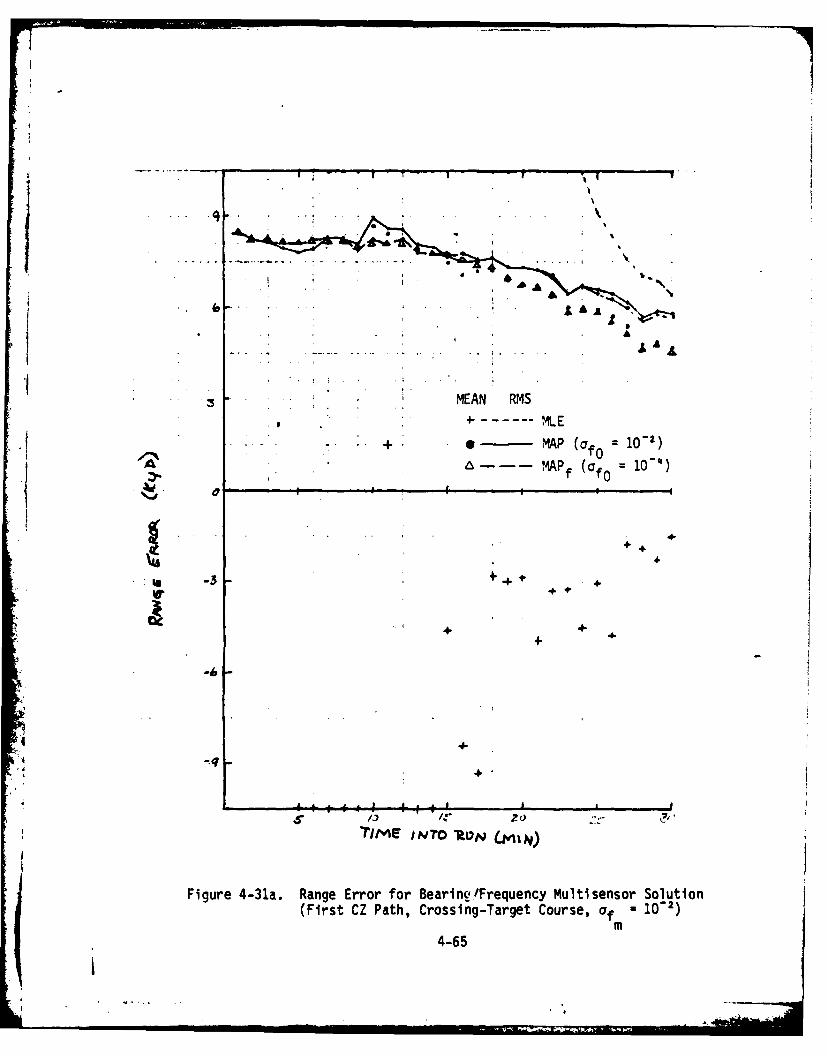
MEAN RMS
.1 + 0MAP (af 10)
A- -MAPf (afo =10_')
0f
+ +.
.+ +
Viq
TIEINTO tON
Figure 4-31a. Range Error for Bearinc,,Frequency Multisensor Solution(First CZ Path, Crossing-Target Course, of - 10-2)
m4-65

. , r II ' I .I" I ' I
... MEAN RMS
I-- MLE. .. .. . .M A P ( O f 1 0 12 )
f 10
MAP. . . . .... I .M A f ( f o 10 )
.4
J_ . 4..Af....At.... .
+1 + +1 +.
4 ir
~+ +
/ 0 -
Figure 4-31b. Speed Error for Bearing/Frequency Multisensor Solution(First CZ Path, Crossing-Target Course, af * 10-2)
4-66
. ., .. .... ....: .. ... .... .. p -
v,, • 0 "; ... .

I,- MAP (af u10'
.1
f% f
0,*
k e+ +
4~~ -'4
TIME INTro RLVAJ&4MIN)
Figure 4-31c. Course Error for Bearing/Frequency Multisensor Solution
(First CZ Path, Crossing-Target Course, of, a 10-1)
4-67

...
--. .' I I .I
MEAN RMS.r , : .. . . .. . . . . . 4 - E Ns
' "-~-*MA P (a =10-2)
- MAP ( 10-4)
.3 ... A , . .A
LA A '' 'A A ' ~
I '& - - • -A AL
I I • y* I I f~
%rymiF wro ALUV C ,iv)
Figure 4-32a. Range Error for Bearing/Frequency Mult sensor Solution(First CZ Path, Crossing-Target Course, ofm 10"3)
4-68
,4 pm I I rI ....

'MEAN RMS" i .W .. . I., . . . ,- . ,- ?S .•~~~ ML" ; + , E
I- . . MAP (af 10 )
of
A.---MAPf (ar 0 O
* , .. . 1 0Sf.
...... . ...... . .. .. .. .. ...
I --0 . .~ , . .. .. .
C "':I . 4 AA -
.. . °. . .. . . ..
I I
,4
I I I I , I,.-IO IS ,'
'rim iO 7ZQA/ 6"w)
Figure 4-32b. Speed Error for Bearing/Frequency Multisensor Solution(First CZ Path, Crossing-Target Course, = 10" )f m
4-69I

4r - - MLE
-- AP (of 10-)
i0
* ~---MAP. (ofo =10T
.. . . . .. .* . -.. .- 4
t&
10-
V.:.. .4 70
i'j
-... .*. . 1* ; I -
.. .a . . . ! i " I MEA ,- l:
Figur.... . CourseiError:- for Bearng/reqenc Multiseor l ution
(First . . C .. Pt, CrsigTre.ore f =1"
. S

values calculated from the algorithms' solutions. The realized solution
accuracy, as demonstrated by the RMS errors plotted in the figures, is gener-
ally improved by the a priori information as used by the MAP algorithm. In
I addition, the inclusion of an accurate center frequency estimate in the a
priori information (the MAPf solution) further improves the solution quality.
The errors in the solutions for the direct-path, closing-course case
(Figures 4-27 and 4-28) are reduced for the most part by both the MAP and MAPf
procedures. Most of the reduction of range error early in the problem comes
from the use of the MAP algorithm; however, later in the run the most signif-
icant reduction comes from the additional use of an accurate center frequency
estimate. Speed and course errors, however, tend to benefit from both through-
out the run. The same case with more accurate frequency measurements
(a fm = 10-) does not benefit from a priori information as greatly. Range and
speed errors show close to zero decrease from the use of MAP, and the course
error improvement is significant only in the early problem stage. For the
direct-path, crossing-course case (Figures 4-29 and 4-30) the MAP procedure
provides improved solution accuracy, again early in the problem. However,
little difference occurs after the first 6 or 7 minutes into the run. The
improvement due to the a priori information again is less for the case with
the more accurate frequency measurements. The first CZ, crossing-course case
again shows improvement in solution accuracy using the MAP and MAPf proce-
dures. The exact relationships among the three procedures are, however, diffi-
cult to see due to the poor convergence of the MLE algorithm for most of the
run.
In general, the a priori information improves solution accuracy to a
greater degree for cases with the more difficult geometries and less accurate
measurements. In other words, the more observable and accurate the solution
is with measurements alone, the less impact any a priori information will
have. It should be noted how well the MAP procedure with accurate center fre-
quency does for all geometries and measurement errors throughout the entire
run. The mean errors additionally show a high degree of average accuracy with
generally very low bias.
4-71

4.3.3 Theoretical Range-Error Lower Bounds
Theoretical lower bounds for the range-error standard deviations are
represented in Figures 4-33 through 4-35 for the simulations run. The plotted
values are the major axes of the position eigenvalues for the inverse psi
matrix computed during the Gauss-Newton solution procedure. These estimates
for range-error lower bounds may represent the relative potential solution
quality achieved from all available information from the different solution
procedures. In addition, although the values are averaged over Monte Carlo
repetition the lower bound estimates are independent of the number of con-
verged repetitions and do not, in actuality, vary significantly between repe-
titions. An indication of the value of a priori information to solution qual-
ity and solution convergence may be observed. The range RMS errors are also
plotted in order to compare the theoretical values to the solution quality
actually achieved by the algorithms. The plotted results again indicate the
value to range accuracy of using the MAP and MAPf procedures over the MLE,
particularly in the cases with the lowest solution quality. Figure 4-33 shows
the reduction in range error bounds achieved from the use of the MAP algorithm
and the accurate center frequency estimate for the direct-path, closing-
course case. The effect is seen to be much lower for the case with greater
frequency measurement accuracy. Relatively little difference is observed in
Figure 4-34 among the different algorithms for the more observable direct-
path, crossing-course geometry. The first CZ, crossing-course case plotted
in Figure 4-35 shows improvement due to the MAP algorithm but very little from
the use of accurate center frequency estimates.
4-72

Si .. . I . RS BOUND
I MAP (f 0 10"2 )' r , MAP 10-4)' II ' ' . . . .
5, .. ,D ./ V ...
+
* (af'
• .! : . ',
4+ " ' I -",V W
! .,4 -. I
.44
,. af... ,...... -. : zs- I I
Av0
u+,+++
'T/Ml F .1 Nto RU N MIA)
... . "RMS BOUND"
. . . . '; , :'.. . ,.-": . '' :. , •MAP (Gf0 : 0 "')
Figure 4-33." Theoretical Lowr Bd oMAP (af 10 )
4e7
Wit Igo';
, 5t o - "a a . ,
Figure 4-33. Theoretical Lower Bound on Range Error for Bearing/FrequencyMultisensor Solution (Direct-Path, Closing-Target Course)
4-73
qxzE

RMS BOUND+ --MIEi .
[10 MAP (af = 102). 7-C • " . - . MAP ( = 10-4)F * e( I - ' " i . ... " f 0
.4 ~ s .. . .. .... . . .
A
16. 20...
S., RMS BOUND0 4 MLE
MA (a =10-2:" .:'. ... • M P ( fo
0 " ' MAP (af = 10- 4)
At
S. -,3
10Is 20 a; 30
TIME ro Ru.w m avFigure 4-34. Theoretical Lower Bound on Range Error for Bearing/FrequencyMultisensor Solution (Direct-Path, Crossing-Target Course)
4-74

4 +~ A 1-.4
* 4 -MLEMAP (yf 0 =10-
2 )
a AMAP (af = 10-)
/00TIM E whro -PON (-MIN)
RMS BOUND ~ 2
.6.
01
* .A
I'.+
4-75.

CHAPTER V
SUMMARY AND CONCLUSIONS
The value of incorporating a priori information into a TMA solution was
investigated as described in Reference 4. The conclusion of that study, based
on Monte Carlo simulations of Maximum Likelihood and Maximum a posteriori
estimates, was that a priori speed information was very beneficial in early
solution performance; however, (crude) a priori range estimates primarily
* aided the initial numerical convergence of the solution iteration procedure.
In effect, the a priori range variance produces a positive definite mean
Hessian matrix which allows numerical convergence.
5.1 IMPROVED ITERATION PROCEDURES
This study examined two procedures for improving solution convergence
during early parts of the prob.lem to ascertain whether the original solution
procedure was optimum. The previous solution procedure iterated towards a
null of the gradient of the a posteriori density function (or likelihood
ratio) using step-size constraints to bound the iteration excursions. In this
study, the procedure was modified to minimize the logarithm of the a
posteriori density function (or the log likelihood ratio) using a line search
along the direction of the Gauss-Newton step. Several useful results were
obtained from that study.
The line search does not always produce convergence to the minimum solu-
N4 tion. At times when observability is poor, the line search occasionally pro-
duces a zero step which would retain the original solution and, therefore, not
incorporate the added measurements. It was found that a heuristic procedure
should be used in that case, which involves taking a limited step in the
Gauss-Newton direction without regard for minimizing the cost function. This
procedure eventually resulted in obtaining a minimum solution. In effect,
5-1

when this procedure is invoked the cost function is not approximately quadra-
tic at the current solution iteration and one must step away from that solu-
tion before proceeding with the normal optimization process.
The modified Gauss-Newton procedure does improve numerical convergence
for both MAP and MLE solutions, but the MAP solution still converges more
often during periods of poor observability. The net cost of incorporating the
line search is increased even though the number of iterations is reduced. The
increased cost is not significant and is within the tolerance of program opti-
mization.
The modified Gauss-Newton procedure does result in a significant improve-
ment in course and speed solutions during periods of poor observability when a
priori range estimates are included. When sufficient data is processed, the
* isolutions converge to the same values regaidless of numerical procedure and
essentially without regard to use of a priori range information.
The other procedure tested was the estimation of an observable (three-
state) relative motion solution on the first leg which is bootstrapped to a
full solution on the second leg. The procedure can be applied with or without
a priori information by using a line search on range during the second leg.
It was found that the relative motion solution can be solved consistently with
little cost because it is observable. It can be coupled with a priori range
or speed information to generate single-leg solutions for tactical informa-
tion. It was found, however, that numerical convergence on the second leg was
not significantly improved by using the bootstrapped solution rather than a
zero-speed initialization. However, the relative motion situation is still a
usefu'l feature because it can be computed along with the full solution and be
used for tactical inputs when the full solution does not converge. One
approach that was not studied was estimation of range by combining relative
motion solutions from individual legs. There were insufficient resources
available to pursue that study but it would be similar to the widely used
Ekelund procedure. In any event, it is recommended that one incorporate a
priori information on the first TMA leg by solving for the relative motion
5-2

solution and combining that with the a priori information in a least-squares
sense. This conclusion is based on numerical convergence behavior of the
three-state and four-state solutions. After the first own-ship maneuver, the
four-state problem should be solved if it converges because the previous rela-
tive motion solution is invalid after a maneuver.
5.2 BEARING/FREQUENCY MULTISENSOR TMA
The using of both bearing and frequency (Doppler ranging) measurements
can allow solution of the TMA problem without maneuvers. In the context of
this study, that problem was examined to ascertain the value of a priori esti-
mates of range, speed and/or base frequency. The multisensor MLE and MAP pro-
cedures generally performed quite well when bearing and frequency measurement
were accurate. For all cases simulated, a priori information provided enhanced
numerical convergence of the algorithm with the use of an accurate center
frequency estimate providing the greatest improvement. The improvement in
convergence was particularly large for the runs which had both the more accu-
rate frequency measurements and an accurate center frequency a priori esti-
mate. Without the latter, the value of the other a priori information was
minimal. The solution accuracy, as measured by the RMS errors, was improved
by both the use of a priori range information and an accurate frequency esti-
mate. However, in this situation the runs with the less accurate frequency
measurements were those which were most improved. This result was reflected
as well by the theoretical range lower bounds on range error standard devia-
tion. Solution accuracy was most enhanced by the a priori information for the
cases with difficult geometries and less accurate measurements.
5-3

APPENDIX
DEVELOPMENT OF GRADIENT COMPUTATIONS FOR BEARING AND FREQUENCY MLE
Assuming that independent Gaussian bearing and frequency measurements
(Bm, fm) are made at discrete times, tk, the log likelihood ratio for the mul-
tiple observations is
N
r (Bi(k) - )B k1
N
(+ 2f F, (fm(k) -k=1
+ log(2=2aa) (1)
where A is the conditional probability density function for the joint measure-
ment sequences, given the solution (x(k)) and the true base frequency (fo).
The target solution vector is contained in B and n.
B~k) = [,1(to) + (tk - to)x3(to) - xlos(tk)1(2
Lx2to) + (tk - to) 4(to) - x2os(tk)J
n(k) 1 - k(k) (3)
A(k) = (x3(to ) - X3os(tk))sin 8(k) + (x4(to ) - ;4os(tk))Cos B(k) (4)
When a priori knowledge of base frequency has a Gaussian distribution, the a
priori information can be incorporated and a likelihood ratio developed which
is conditional only an x. Note:
A P{B f (5)1 f
0!

Then, if Pfo(f0) is the a priori probability density for f 0
Alp lPf (f0 )df 0
p P{Bm~Ix ffmI/x (6)
Pff I/X f Pl{./, Pfo (f0 )df 0 (7
for
p ~ ) 1 g (f 0 _ f ) 2
P0 (f 0 N2-wf e -2cf70(8
and
Pff I/x e-(fm - fn) (9)
m (2waf)N/2 2qo(9
then
(0)
=f ( 2 aZN/.x fe- df 0(10)
0
I~f N (f (k) -f 0(k)) 2 (f 0 f)2 (1
k=1 fa
.4 N f2(k) ~
1(f0)= r f + f4.+ t3n(k)
* - o + N fm(k )T(k) fo (20 fk=1

(fo-f)2 N f(1(k3 )10 fo
0: 00 0I(fo - + -f + -2 -- (13)f~ k =1 f f0 0 f
where O( N:To + E fm(k)ln(k)fo k=lfo a2 (14)
f+ E n(k)
ao k=1
is the a posteriori mean and therefore the least squares estimate of fo" ItsI conditional variance (given x) is
2a -a^ (15)
J- 2 N
Oz a (k)fo k=1
Note:2
ef Na fofo o T I (fm(k) - Ton(k))n(k) (16)o T o + f k = 1
Equation 13 can be manipulated to an alternate form:
a a 2
(f) (f -f) N (fm(k) -fo(k))' (fo 0 fo ) '17
fo k =10
The integral in Equation (10) over fo can be computed as
1 C°ox (fm(k) f+ 0ko- O)
Pf }Ix (2 N2af) /2 fo fo ) (18)
3
ii.

The log likelihood ratio for x is therefore
N
-ZnhV = z 1 (Bm(k) " B(k)) 2
k=1
N+ 7 (fm(k) - ))2
k=1
+(19
+a fo0 - 'o)2
.9n + ,-frn-(k (19)! fo k=1
with NF4 (fm(k ) - on(k ))n(k )
k=o + 2k= N (20)
-F- (~nk)f0 k=1
The last term is much less sensitive to x than any other term and can be con-
sidered to be constant. The gradient of JLR = -ZnA', with respect to _
is therefore
N
VXJLR or EB (Bm(k) B(k))VxB(k)B k=1
rNI
(fm(k) -^ f0n(k))Vxr1(k)]
+ (k)(fm(k) - f0 (k))k=11 ' 4

Of -o )I Vx (21)f 0 o 0 f Xo0 J
The last term can be shown to be identically zero. Thus:
N (B~)-8(k))
VxJLR = [E - Vk _B(k)- k=1 C
f (Im (k) - 0 n(k))+ o 0 V xn(k) (22)
f
The second gradient of JLR is
N VxB(k)VXB(k) N (B B) T^
VxVx LR E a o _k=1l k=1 B
N
+f 4 : v Xn(k)V>1n(k)
k-1
v'f N
E (f - 2f 0 qlk))V x nlk)
k-1
f N0 E (fm(k) f^n(k))(VxVxn(k)) (23)
I
i5

withN (fm(k) - 2f on(k))Vxn(k)
Vxf= f N.- (24)
k=1 + E rn2 (k)
o k=1
The expected value of the second gradient is required for the Gauss-Newton
procedure. Under the assumption that x is correct, then one can compute after
tedious algebra:
E{x x LRI
N
k=1 -
B F, + A~ V f(k T k
' =~~k1 -k--
+ aS[af
( j r vxnu) ( k)V x n(k)
- p(k) + Uaf- Ik=I 0_
+
6
I...

N
E n(k)VXV n(k)k=1S(25)
n20 + af
j=1 fo
The last two terms can be dropped because they are inconsequential when com-pared to the others when of/fo is small (e.g., of the order of It/c). The equa-tion can be simplified without hampering convergence to
N
LR Vxk(tk)VxBGtk)Ik=1 - -
i+
N (26)
4 The term in brackets is positive semidefinite, since all quadratic forms
reduce to
N2N ~ n(k)a
k k=1
Cfok ~ k- 0 i2k
7

where ak is the projection of any vector on VxI. This quantity is zero onlyk xfor a vector which is orthogonal to the gradient at all time steps. Otherwise
this quantity is positive. The second term in brackets represents the infor-
mation lost by not knowing the actual base frequency. If of>>Of or when N
becomes sufficiently large, this information loss disappears.
The gradients of B and I must be evaluated.
A-(t [ x1(t°) + (t - 0 3 (t o)- los(k) (27tk) t [x2(to) + (tk to)x4(to) x2os(tk)] (27)
A(tk) = (x3(to) - x3os(tk))sin B(tk) + (x4(to) - x4os(tk))cos B(tk) (28)
cos i(tk)
VxI(t 0)B(tk) 1~ B(t k A (29)
~(tk- t)sin A~k
A0
Vx(to) (tk) sin(tk . to)r xt)(tk) (30)-Ntke)sin xits
A
cos B(tk)
4m
Vcr (x3(tO) - X3os(tk))cos Bitk) - (x4(tO) - X3os(tk))sin 8(tk) (31)
S!The modified Gauss-Newton solution for the step In x is1
Ax = -a*-1V J = ax (32) 1
8

The projection of this step along the gradient is
'aXTVj -aVJ*-,v = -a TV,
N=a[ Tf + N k (k= (33)
nf _ (k) +
k=1f0
with
vTk :SVBkx (34)
and
=VTA Ax &4 + v AB(5k x k-!o v cr (5
) M = X3 sin + Ax4 cos B (36)
A = (afc)/f o (37)
Unless both ABk and k are zero at every time step, the projection is always
positive.
The accuracy of the base frequency estimate (f0 ) depends on both error in
the measurement and error in the solution (x). Let f0 be the true center fre-
quency and wk be the frequency measurement error. Then
NEf (f,(k) -+o;(k) (,)
fo 0" fo -Tro f fo + f N.4(38)
+ kof0 k=1
9

N
T ro o+ f + fon(k) - o(Tn(k)
gk=lf 0 2 N (9
• ( o - o f -W
2 N
-f f) .4. + 1:(wk - T0 (ri(k) - (kf)r(k)f o f k=1 (40)
a f2
fo k=land
fOf N f2 (41)
12(k) + 7
k=l 0
Swhere N n(k)%xA(k)
q k=1 (42)
N q^a22 of
tk=10 0
101
- ,e J ,

REFERENCES
1. Chou, S. I., Exploitation of Environmental Data Knowledge in Surface Ship
ASW Target Motion Analysis, PM-4 Study Proposal, March 1978.
2. Chou, S. I., Anti-Submarine Warfare (ASW) Passive Target Tracking, Naval
Ocean Systems Center, January 1980.
3. Hartley, H. 0., "The Modified Gauss-Newton Method for the Fitting of Non-
Linear Regression Functions by Least Squares," Technometrics, Vol 3,
I No. 2, May 1961.
4. Jarvis, H. F., and N. B. Nill, Target Tracking with Multiple Data Sources,
Analysis and Technology, Inc., 15 August 1979.
R-1

Distribution List for
Target Motion Analysis with A Priori Information
No. of Copies
Defense Technical Information Center 12Bldg. 3, Cameron StationAlexandria, VA 22314
Office of Naval ResearchDepartment of the NavyArlington, VA 22217
(Attn: Mr. J. G. Smith, Code 411SP) 2
DirectorNaval Research LaboratoryWashington, D.C. 20375
(Attn: Code 2627) 1
Naval Ocean Systems Center271 Catalina BoulevardSan Diego, CA 92152
(Attn: Dr. P. Reeves, Code 632) 1(Attn: Dr. J. Zeidler, Code 6212) 1
Naval Underwater Systems CenterNew London LaboratoryNew London, CT 06320
(Attn: Dr. C. G. Carter, Code 3331)
Naval Sea Systems CommandNavy DepartmentWashington, D.C. 20360
(Attn: Mr. D. Porter, Code 63R11) 1(Attn: Mr. C. Marin, Code 63R16) 1
Naval Electronic Systems CommandNational Center Building No. 1Washington, D.C. 20360
4 (Attn: Mr. J. Schuster, Code 612) 1
Naval Surface Weapons CenterWhite Oak LaboratorySi lver Spring, MD 20910Code U-20 1
Defense Advanced Research Projects Agency1400 Wilson BoulevardArlington, VA 22209 1
t I

Distribution List (cont'd)
No. of Copies
.Massachusetts Institute of TechnologyLaboratory for Information and DecisionSystems
Cambridge, MA 02139 1
Commander, Submarine DevelopmentSquadron 12
* IBox 70Naval Submarine Base, New LondonGroton, CT 06340
Office of Naval Research Branch Office
Building 114, Section D
666 Summer StreetBoston, MA 02210
Dr. Harold A. TitusNaval Postgraduate SchoolDepartment of Electrical EngineeringCode 62TSMonterey, CA 93940 1
Naval Underwater Systems CenterNewport, R.I. 02840Code 352 1Code 351 1
Naval Intelligence Support CenterSuitland, MD 20390Code 20C 1
9.

Jr