AD-A227 473WRDC-TR-90-2020Volume 11

ADVANCED STRUCTURAL INSTRUMENTATION

Volume I1

A. J. DennisGraham B. FultonUnited Technologies Research CenterEast Hartford, Connecticut

Final Report for Period Feb. 83 - Nov. 89

,N&

Approved for public release; distribution unlimited.

AERO PROPULSION AND POWER LABORATORIESWRIGHT RESEARCH DEVELOPMENT CENTERAIR FORCE SYSTEMS COMMANDWRIGHT PATTERSON AIR FORCE BASE, OHIO 45433-6563

6 4

NOTICE

WHEN GOVERNMENT DRAWINGS, SPECIFICATIONS, OR OTHER DATA ARE USED FOR ANYPURPOSE OTHER THAN IN CONNECTIPN WITH A DEFINITELY GOVERNMENT-RELATEDPROCUREMENT, THE UNITED STATES GOVERNMENT INCURS NO RESPONSIBILITY OR ANYOBLIGATION WHATSOEVER. THE FACT THAT THE GOVERNMENT MAY HAVE FORMULATED OR INANY WAY SUPPLIED THE SAID DRAWINGS, SPECIFICATIONS, OR OTHER DATA, IS NOT TOBE REGARDED BY IMPUCATION, OR OTHERWISE IN ANY MANNER CONSTRUED, AS UCENSINGTHE HOLDER, OR ANY OTHER PERSON OR CORPORATION; OR AS CONVEYING ANY RIGHTS ORPERMISSION TO MANUFACTURE, USE, OR SELL ANY PATENTED INVENTION THAT MAY IN ANYWAY BE RELATED THERETO.

THIS REPORT HAS BEEN REVIEWED BY THE OFFICE OF PUBLIC AFFAIRS (ASD/PA)AND IS RELEASABLE TO THE NATIONAL TECHNICAL INFORMATION SERVICE (NTIS). ATNTIS IT WILL BE AVAILABLE TO THE GENERAL PUBUC INCLUDING FOREIGN NATIONS.

THIS TECHNICAL REPORT HAS BEEN REVIEWED AND PS APPROVED FOR PUBUCATION.

WILLIAM A. STAGE I:AK J. fRSHONProject Engineer Technical Area ManagerComponents Branch Components BranchAero Propulsion and Power Aero Propulsion and Power

Laboratory Laboratory

FOR THE COMMANDER

ROBERT E. HENDERSON

Deputy for Technology

Turbine Engine Division

Aero Propulsion and Power

Laboratory

IF YOUR ADDRESS HAS CHANGED, IF YOU WISH TO BE REMOVED FROM OUR MAILINGLIST, OR IF THE ADDRESSEE IS NO LONGER EMPLOYED BY YOUR ORGANIZATION PLEASENOTIFY wgnc/PnTc WRIGHT-PATTERSON AFB, OH 45433- 6563 TO HELP MAINTAINA CURRENT MAILING UST.

COPES OF THIS REPORT SHOULD NOT BE RETURNED UNLESS RETURN IS REQUIRED BYSECURITY CONSIDERATIONS, CONTRACTUAL OBLIGATIONS, OR NOTICE ON A SPECIFICDOCUMENT.

Unaci j ; sif ledSECUR17Y CLASSIFICATION OF THIS PAGE

REPORT DOCUMENTATION PAGE F0VE No 070-018-, P~OORT SECURITY CLASSIFICATION 1b. RESTRICTIVE MARKINGS

tV_C .A SSIFIFD______________________21i :17"UP1Ty CLASSIF CATION AUTHORITY 3 DISTRIBUTION/ AVAILABILITY OF REPORT

N/CAFCT/DNGAIGSHUL Approved for Public Release. Distribution,___________________________________SCHEDULE_ IUnlimrnited

4 r-r0P3F!NG ORGANIZATiON REPORT NUMBER(S) 5. MONITORING ORGANIZATION REPORT N'JMBER)

k--,-2330 WRDC-TR-90-2020. Vol. 11

%'AE QFi PERI'CR~IVNr3 ORGANIZAT ON 16ci OFFICE SYMBOL 7a NAME OF MONITORING ORGANIZATION

It~td 'Fechnolo-ies Research ItI appI~cablel Aero Propulsion and Power Laboratory (WRDC/triterPOTC) Wright Research Development Center

SS'R 5'Ct, State and ZIP Code) 7b ADDRESS (City, State, and ZIP Coca)

S',er Lanie

F ist Hartford CT 0610S WPAFB3 OH 45433-6563ta'AVE 3 FUN DINAG. SDONSOP NG 8oOFFICE SYMBOL 9. PROCUREME. IT INSTRUMENT IDENTIFICATION NUMBER

'.- CAlIZAT,ON (if applicable)

:, Propulsion aind Pow&er POCF3361583C 33i h orarory I

Aj, UPESS City State and ZIP Code) 10 SOURCE OF FUNDING NUMBERS

W < C'POCPROGRAM PROJECT TASK 0ZOR1< UNITELEMENT NO NO INO. COSIN NO

\VP.\FB OH 4-5433-6563 62203F1 3066 12 9T _E 'rnc-ci Secjity ClassifiCationj

~\ DANCED STRUCTURAL INSTRUMENTATION. VOL. 11ALA -iR(S) A. J. Dennis and G. B. Fulton

.PF CF REPORT 13b TIME COVERED 14. DATE OF REPORT (Year. Month bay) 15 PAGE COUNT

I , 'Ar I FROM Feb 83 TO Nov 89 11 90/06/1117[6 ';LR4-EMENTARY NOTATION

SS.~A.i-1 CODE 18 SUBJECT TERMS (Contnue on reverse if necessary and iaentify by blocki number)

05P Instrumentation, Static strain, Strain measurement.

Temperature measurement. Sensors, Turbine measurementsj ABSTRACT (Continue on aeverse if necessary and identify by block number)

This report presents the results of the development and test of a variety of steady-state strain andtemperature sensors specifically aimed at application in hot sections of advanced gas turbines. In each

* case, the sensors have shown success in the laboratory, and tests and results described herein weredesigned to simulate thre actual turbine environment. Most of the testing was carried out in the UTRCvaIcuum spin rig which was able to achieve speeds and temperatures characteristic of advanced gastUrbines. Volume I is an overview of the sensors, physical description, summary comparison of resultsand conclusions and recommendations. Volume 11 gives the details of the sensor fabrication and instal-lation as well as evaluation of the data acquired. The report is divided into the sections each of which'lives the details of a specific sensor tested in this program.

(Continued)2, ,5RiBUTION/AVALABILITY OF ABSTRACT I 21. ABSTRACT SECURITY CLASSIFICATION

x- U L ZE/NME ,., AS RPT - rIC usE-s Unclassified22a INAME OF RESPONSIBLE INDIVIDUAL 2b. TELEPHONE (Include Area Code) 22c OFFICE SYMBOL

DD Form 1473, JUN c'Previous editions are obsolete SECURITY CLASSIFICATION OF THFS PAGE

UNCLASSIFIED

SECURITY CLASSIFICATION OF THIS PAGE

CONTINUATION from DD Form 1473, Block #19.

/. Temperature sensors tested in the present program include conventional wie thermocouples

and an advanced type of thin film thermocouple deposited directly on the test piece. The temperature

measuring capability of twin core optical fiber sensor technology has also been demonstrated. Remotesensing of temperature was achieved with a thermographic phosphor technique, and optical pyrometrywas used as a control throughout the program. Additionally, the feasibility of advanced concept heat

flux sensors on a turbine blade was demonstrated.

Advanced strain gages were also tested. Two types of wire strain gages were bonded to the tur-

boin, disk. the first, a conventio,,.a .,,n,.y avaii .'ickel-Chrome alloy type. and the other. a

modified FeCrAI alloy developed by the Chinese. Strain was also measured with several types of sput-

tered thin film sensors as well as the twin core optical fiber sensor. Speckle photogrammetry was used

for noncontacting strain measurement throughout the spin rig testing.

Ae -3,.iCi For

14TIS GFA&t!:TIC TABUnannouncedjustification

SBy

niz-tribut Ion

Availability Codes

Avail and/or

Dist Special

DD Form 1473, JUN 86 Previous editions are obsolete

UNCLASSIFIED

CONTENTS

SectionP

LIST OF TABLES ................................................... vi

LIST OF FIGURES ................................................. yji

1. INTRODUCTION ................................................... I-1

I. STRA(N MEASUREMENT BY SPECKLE PHOTOGRAMMETRYOF ROTATING OBJECTS ........................................... 2-1

1. INT RO D UCTIO N ................................................. 2-12. INTERFEROMETRIC PHOTOCOMPARATOR ..................... 2-23. MATHEMATICAL THEORY ...................................... 2-44. PHOTOCOMPARATOR PROCEDURE ............................ 2-75. BUILD I - SPECKLE PHOTOGRAMMETRY ...................... 2-86. DATA PROCESSING .............................................. 2-117. D ISC U SSIO N ..................................................... 2-148. CONCLUSIONS AND RECOMMENDATIONS FROM BUILD 1 ..... 2-169. ADVANCED STRUCTURAL INSTRUMENTATION

BUILD 2- SPECKLE PHOTOGRAMMETRY ....................... 2-1810. DATA PROCESSING .............................................. 2-1911. D ISC U SSIO N .. .... ..................... ....................... 2-24

III. HEAT FLUX SENSORS .............................................. 3-1

1. SU M M A RY ....................................................... 3-12. INTROD UCTION ................................. ............... 3-13. DESCRIPTION OF SENSORS ..................................... 3-24. FABRICATION OF SENSORS INTO THE BLADES ................. 3-45. CA LIBRATIO N ................................................... 3-66. TEST R ESU LTS .................................................. 3-107. CONCLUSIONS AND RECOMMENDATIONS ..................... 3-128 R EFEREN CES ................................................... 3-12

ill

CONTENTS (CONTINUED)

Section

IV. FIBER OPTIC SENSORS ............................................ 4-1

1. INTRODUCTION ............................................... 4-12. BA C KG RO U ND .................................................. 4-13. SENSOR CONCEPT AND DEVELOPMENT ....................... 4-44. NONROTATING RISK REDUCTION TESTS-THE

FERRIS WHEEL EXPERIMENT .................................. 4-125. ROTATING TESTS-THE SPIN RIG EXPERIMENT ................ 4-226. D ISC U SSIO N ..................................................... 4-33

APPENDIX A FERRIS WHEEL DATA BASE ....................... 4A-1

V RESISTANCE STRAIN GAGES ....................................... 5-1

1. INTRO D U CTIO N ................................................. 5-12. O BJE C T IV E ...................................................... 5-13. STATE OF THE RESISTANCE STRAIN GAGE ART ................ 5-24. APPROACH TO DEMONSTRATION TEST ........................ 5-45. DEMONSTRATION TESTS OF THE FeCrA BHP-700C

W IRE STRAIN GAGES ........................................... 5-66. DEMONSTRATION TESTS OF THE PdCr SPUTTERED-FILM

ST RA IN G ,' G ES .................................................. 5-187. CONCLUDIP'G REMARKS ....................................... 5--408. ACKNOWLEDGEMENTS ......................................... 5-419. BIBLIOGRAPHY ........................ 5-41

VI. TEST FACILITY .................................................... 6-1

1. A B ST RA C T ...................................................... 6-12. INTRO D UCTIO N ................................................. 6-13. SPIN RIG DESCRIPTION ......................................... 6-24. MODIFICATIONS FOR HEATED TESTS ......................... 6-75. TEST HA RDW ARE ............................................... 6- 146. DATA ACQUISITION SYSTEM .................................. 6-157. TEST PROCEDURE .............................................. 6-218. CONCLUDING REMARKS ....................................... 6-229. R EFE REN C E ..................................................... 6-22

APPENDIX A DATA ACQUISITION SYSTEM COMPONENTSPECIFICATIO NS ................................................ 6A -1

VII. DISK STRESS ANALYSIS ........................................... 7-1

iv

TABLES

Table

1. Speeds and temperatures at which data were taken ..................... 2-11

2. Tsss measured sensor response (unattached devices) .................... 4-12

3. Sensor inventory; Ferris wheel experiment ............................. 4-17

4. Instrumentation; Ferris wheel experiment ............................. 4-17

5. Load and strain relation ............................................. 4-19

6. Spin rig sensor parameters ......................................... 4-24

7. Analytically predicted, unattached calibration constants and response(per inch of sensor length) ........................................... 4-25

8. Test summary spin test of wire-form static strain gages ................. 5-11

9. Test summary static test of sputtered-film static strain gages ............ 5-26

1M. Test summary spin test 2; sputtered-film static strain gages ............. 5-30

11. Test summary spin test 3; sputtered-film static strain gages ............. 5-37

V

FIGURES

2-1. Protocomparator block diagram. .................... 2-3

2-2. Specklegram schem atic ................................................ 2-4

2-3. O ptical arrangem ent in spin rig ......................................... 2-9

2-4. Laser control schem atic . .............................................. 2-10

2-5. Build 1 strain vs. speed squared, 300 K .................................. 2-12

2-6. Build I strain vs. speed squared, 422 K ............................ 2-13

2-7. Build 1 strain vs. speed squared, 589 K .................................. 2-13

2-8. Build I ;train vs. speed squared, 755 K .................................. 2-14

2-9. Build I effect of gage length on measured strain for varioustem peratures . ........................................................ 2-17

2-10. Build 2, strain vs. speed squared. Ambient temperature, clockwisero tation . ............................................................. 2-25

2-11. Build 2, strain vs. speed squared. Ambient temperature,counterclockwise rotation .............................................. 2-25

2-12. Build 2, strain vs. speed squared. 422 K temperature,counterclockwise rotation .............................................. 2-26

2-3. Build 2, strain vs. speed squared. 589 K temperature,counterclockwise rotation ........................................ 2-26

2-14. Build 2, strain vs. speed squared. 755 K temperature,counterclockwise rotation ........................................ 2-27

2-15. Build 2, strain vs. speed squared. 950 K temperature,counterclockwise rotation .............................................. 2-27

3-1. Schematic of the embedded thermocouple heat flux sensor ................ 3-3

3-2. Schematic of the Gardon gauge heat flux sensor .......................... 3-4

3-3. High intensity qvi3rtz lamp bank ................................ 3-7

Vi

FIGURES (Continued)

3-4. Airfoil positioned in quartz iamp rig with water-cooled shields -bottom view . ......................................................... 3-7

3-5. Airfoil positioned in quartz lamp rig with water-cooled shields - sidev iew . . . . . . . . . . . . . . . . . . . . . . . . . . . . . . . . . . . . . . . . . . . . . . . . . . . . . . . . . . . . . . . . . 3 - 8

3-6 . H igh intensity quartz lam p rig .... .................................... 3-9

3-7. Calibration data for embedded thermocouple sensor ...................... 3-11

3-8. Data from mo sensors from the advanced structural instrumentationsp in te st . . . . . . . . . . . . . . . . . . . . . . . . . . . . . . . . . . . . . . . . . . . . . . . . . . . . . . . . . . . . 3 - 1 1

3-9. AC noise level on heat flux sensor output ................................ 3-13

3-10. Leadwire failure at airfoil exit ........ ............................ 3-13

3-11. Failure of leadwire external to airfoil .................................... 3-14

4-1. Fiber optic strain sensor. Typical engine layout ........................... 4-2

4-2. Fiber optic strain sensor. Disk environment .............................. 4-2

4-3 Opr--:,I fibe- ensnr technc!" ' develop.2.n:. ........................ 4-5

4-4. Twin-core fiber optic sensor concept .................................... 4-6

4-5. Strain and temperature response . ...................................... 4-6

4-6. Instrum entation concept ............................................... 4-7

4-7. Twin core optical fiber sensor. Germanium-doped silica sensor withalum inosilicate com pressive layer ....................................... 4-9

4-8. Apparatus for metal coating . .......................................... 4-10

4-9. Fiber optic strain sensor. Multi-mode output fiber cross section .......... 4-10

4-10. Fiber optic strain sensor. Basic optical unit design ........................ 4- 11

4-11. Fiber optic strain sensor. Fully assembled sensor using fusion-splicetechnique . ...... ........ ............................................ 4-12

4-12. Comparison of measured and computed strain sensitivity. ................ 4-13

Vii

FIGURES (Continued)

4-13. Twin-core fiber optic sensor. Predicted and measured temperaturesensitivity ...................... ............. ...... ............. 4-13

4-14. 1win-core optical fiber sensor. Ferris wheel experiment: F 1Wn) disk ......... 4-i4

4-15 Fiber optic strain sensor. Attachment study ......... ............. 4- 1P

4-16. Fiber optic strain st-nsor. Attichment study (sample I0A-2GA-1fW)). ............................................. .. 4-10

4-17. Sensor array. Ferris wheel experiment ...................... 4-10

4-18. Twin-core optical fiber sensor. Ferris wheel Experimental Facility. ...... 4- 1

4-19. Ferris wheel test program ....................................... 4-20)

4-20. Twin-core optical fiber sensor. Temperature response. Ferriswheel data: run No. 4, sensor 6, 633 nm .................... ............. 4-20

4-2 1. Twin-core optical fiber sensor. Load response at 589 K. run No. 4,sensor 6, 633 nm . .................................... ................ 4-21

4-22. Twin-core optical fiber sensor. Temperature response. Ferris wheeldata: run No. 10. sensor 6, 830 nm . ..................................... 4-21

4-23. T"in-core ontical fiber sensor. Load response at 933 K. Ferriswheel data: run No. 10, sensor 6. 830 nm ................................. 4-22

4-24. Twin-core sensors. Ferris wheel test: modified F100 disk with

sensors N o. 6, 5, 4 ..................................................... 4-23

4-25. Detailed empirical model. Calibration constants ......................... 4-26

4-26. Detailed empirical model. Crosstalk vs. wavelength: WPB No. 6,L = 38.6 mm, OD = 186 mm, spectran No. 4 ............................ 4-26

4-27. Detailed empirical model. WPB No. 6; L = 38.6 rm, OD = 186 rm,spectran N o. 4 . .......................................... ............ 4-27

4-28. Detailed empirical model. WPB No. 6; L = 38.6 mm, GD = 186 mm,spectran N o . 4 . ....................................................... 4-27

4-29. Detailed empirical model. Strain and temperature sensitivity

coefficients. WPB No. 6; L = 38.6 mm, OD = 186 mm, spectran No. 4 .... 4-28

Viii

FIGURES (Continued)

,1-30. Twin-core optical fiber sensor. Temperature response: WPB No. 6,

u n attac h ed . ...... .... .. ..... .. ... ...... ................ .. .......... 4 -29

4-31. Twin-core optical fiber sensor. Flame-spray attachment toM odified Fl(W) turbine disk . .... .................................. 4-29

4-32. Twin-core optical tiber sensor. Miniature 2 - & transmitter,c rs io n1 I. .. .........................................................4 -3 1

4-33. '1vin-core optical fiber sensor. Miniature 2 - x transmitter,c rsio n 2. . .................... .......................................4 - 3 1

4-34. lvwin-core optical fiber sensor. Miniature 2 - x receiver ................. 4-32

4-35. Twin-core optical fiber sensor. Spin rig experiment ....................... 4-32

4-36. Spin rig test program. Build 3/4 B . ..................................... 4-33

4-37. T,in-core optical fiber sensor. Temperature response at (IOX)r/m in. Spin riW data, run No. 5, 830 nm .................................. 4-34

4-38. Twin-core optical fiber sensor. Load response at 422 K. Spin rigdata: run N o. 5, 830 nm ................................................ 4-34

4-39. "win-core optical fiber sensor. Load response at 589 K. Spin rigdata, run N o. 830 nm .................................................. 4-35

4-411. Sensor comparison 152 mm radius, 660E r/min ........................... 4-36

4-41 Sensor comparison. Twvin-core and speckle data superposed ............. 4-38

4-42. Sensor comparison. Twin-core and speckle data superposed ............. 4-38

4A -1. Twin-core optical fiber sensor .......................................... 4A -3

4A-2. Twin-core optical fiber sensor .................................. ....... 4A-4

4A-3. Twin-core optical fibei sensor .......................................... 4A-5

4A -4. Twin-core optical fiber sensor .......................................... 4A-6

5-1. The wire strain gage configuration used is 3 millimeters by 3 millimeters. .... 5-3

5-2. Metallurgical instability data for five strain gage alloys .................... 5-3

Ix

FIGURES (Continued)

5-3. Change in resistance vs. temperature after different soak times at1250 K for a samplk FeCrAI Alloy (Fe-I lCr-12A]) . .... ................. 5

5-4. Change In rNs:stance vs. temperature afier different soak times for asample PdCr alloy (Pd-16Cr-8C) ..................................

Pretest photo befo rc 950 K spin test 2................................

5-6. Gage factor vs. temperature for one of four wire strain gagesmounted on a cantilever bend test bar of Inconel 71. . .................... . S

5-7. Apparent strain vs. temperature during cttd-down for oie ofthree wire strain gages mounted on a flat rectangular test bar ofIN IW(W turbine disk m aterial . ........................................... 5

5-8. Temperature vs. time for four cooldown rates for which apparentstrains w ere m easured . ................................................ .

5-9. Detailed photo after the 950 K spin test 2. The wire gage installationshows no visible m ajor deterioration . ................................... ;-11)

5-1)a. Spin test strain data obtained at 165 millimeter radius, versus r/min ........ 5-13

5-1Ob. Conclusion of data at 165 millimeter radius .............................. 5-14

5-1 la. Spin test strain data obtained at 152 millimeter radius, versus r/min ........ 5-15

5-1 lb. Conclusion of data at 152 millimeter radius .............................. 5-16

5-12. Four thin-film gages mounted on a test bar for gage factor testing .......... 5-19

5-13. Good strain transfer is demonstrated in tension (+) and compression(-) from the test bar to the welded gages ............................ 5-21

5-14. Pretest photo of the turbine disk installed in the P&W heated"Ferris wheel" rig for static radial loading tests .............. ............ 5-21

5-15. An example of catastrophic delamination of the Si3N4 sputteredinsulation at 950 K during a preliminary trial of the foil-mountedgages on a turbine disk . ............................................... 5-22

5-16. Pretest photo before 95(0 K static Iferris wheel test ........................ 5-21

5-17. Measured strain vs Ferris wheel radial load ........................... 5-23

FIGURES (Continued)

5-18. Post-test photo after the 950 K static Ferris wheel test ................. 5-2-5

5-19. Detailed pretest photo before 95G, K spin test 2 ........................... 5-27

5-2). Post-test photo after the 950 K spin test 2 ............................... 5-28

5-21. Detailed pretest photo before 950 K spin test 3, beforecem enting of lead w ires . ............................................... 5-33

5-22. Pretcst photo hcore 950) K spin test 3 of the completed installationof the o vercoatcd thin-film strain gages . ................................ 5-34

5-23. Pot-test detailed view of the overcoated thin-film strain gagesafter 951) K spin test 3 . ................................................ 5-35

6--1. Overall view of UTRC spii rig . ..................... .................. 6-2

6-2. UTRC spin rig cross-sectional schematic .............................. 6-3

,-3. Drive spindle and bearing support system ............................. 6-4

6-4. Spin rig fluid system s .......................................... ....... 6-6

6-5. Section through the hot cham ber . ...................................... 6-8

6-6. Induction heater load cell .............................................. 6-8

6-7. Uncooled rotating junction can configuration for Build 1 .................. 6-10

6-8. Water c(x)led junction can with labyrinth shield ............ ......... 6-11

6-9. Final configuration of junction can ...................................... 6-12

6-10. Comparison of disk and junction temperatures ........................... 6-13

6-11. Cross-sectional view of a test rotor . .................................... 6-15

6-12. D ata acquisition schem atic . ........................................... 6-16

6-13. Strain gage bridge arrangement ......................................... 6- 17

6-14. Test sequence for static strain . ......................................... 6-19

7-1. H PT m od ule . ........................................................ 7-2

xi

FIGURES (Concluded)

7-2. Cross-sectional view of test rotor ....................................... 7-3

7-3. Finite element model of spin test disk ................................... 7-3

7-4. Assumed disk tem perature gradients .................................... 7-4

7-5a. Radial strain at gage locations vs. thermal gradient, 13,2)f r/min ......... 7-4

7-5b. CIRC strain at gage locations vs. thermal gradient, 13,2(Wl r/min ............ 7-5

xjj

I. INTRODUCTION

The new generation of gas turbines being introduced into service are operating at unprecedented

levels of temperature and speed, levels which are dictated by the demand for improved performance

and reduced fuel consumption. At the same time, it is required to achieve the higher levels of

performance \kith no degradation of durability. The materials used in the hot section environment of

these engines are working in a regime wN here small changes in temperature or stress have large effects

on component life. We must. therefore, develop instrumentation technology to accurately and reliably

measure strain and temperature in the hostile turbine environment so that component life may be

accurately predicted.

This report presents the results of the development and test of a variety of sensors specifically

aimed at application in the hot sections of advanced gas turbines. In each case, the sensors have shown

success in the laboratory, and the tests and results described herein were designed to simulate the

actual turbine environment. Volume I is an overview of the sensors, physical description, summary

comparison of results, and conclusions and recommendations. Volume II gives the details of the

sensor fabrication and installation as well as evaluates the data acquired. The report is divided into the

sections tabulated below, with the principal authors, each one of which gives the details of a specific

sensor tested in this program.

SECTION TITLE AUTHOR

I Introduction

II Speckle Photogrammetry K. Stetson, UTRC

III Heat Flux Sensors R. Strange, W Atkinson, P&WA

IV Fiber Optic Sensors J. Dunphy, UTRC

V Resistance Strain Gages H. P. Grant, W L. Anderson,

J. S. Przybyszewski, P&WA

VI Test Facility A. J. Dennis, G. Fulton, UTRC

VII Disk Stress Analysis G. Fulton/T. Vasko, UTRC

1-1

11. STRAIN MEASUREMENT BY SPECKLE PHOTOGRAMMETRY OF ROTATINGOBJECTS

1. INTRODUCTION

a. Technical Concept -- Speckle photogrammetry is a noncontact method to measure strain

particularly useful at high temperatures. The technique involves illuminating the sample with laser

ligoht and photographically recording its image through a telecentric lens system. The random

scattering of the laser light by the object surface causes a speckle pattern to form in the photographic

image that uniquely identifies each area on the object surface. A heterodyne interferometer is used as a

high precision photocomparator to measure small differential displacements between pairs of

photographs (specklegrams). Comparison of specklegrams taken before and after a stress is applied to

an object can reveal two-dimensional strain patterns over a substantial sui .ace area. This technique

has a definite advantage in the study of objects at high temperatures because the surface of the object

itself is measured without any strain sensor materials having to be bonded to it.

Previous work has demonstrated that this technique can be applied with good results on

laboratory samples up to 1140 K. Two-dimensional strains have been measured up to 1.4 percent with

accuracies of a few hundred microstrain and gage lengths of 5 mm (0.2 in.).

b. Application to Rotating Components - Basic Approach-The first problem to be faced in

applying speckle photogrammetry to rotating objects is how to deal with the rotational motion of the

object. One solution is to photograph the object through an image derotator, which can be set to

remove the rotational movement. Certain practical difficulties arise with this approach, however, in

that axial illumination and viewing of the object are required. This further requires that the center of

rotation be at the center of the image field. Because of the limited amount of resolution of the image

derotator, it is impossible to obtain an effective closeup of an eccentric segment of the object.

An alternative is to record a direct image of the object at the radius desired and employ a very

short laser pulse to stop the image motion. As an example, an object point at a 300-mm radius, rotating

at 11,000 r/min, will translate 7 gm during a 20-nsec Q-switched laser pulse. This is less than the

resolution limit of an f/20 imaging system. The next problem that is encountered is synchronization of

2-1

the laser firing so that the object is in the same position with respect to the optical system on each

successive exposure. This synchronizaiton may be achieved to within a few microseconds, and the

object position can be held to within a millimeter or so, which is adequate.

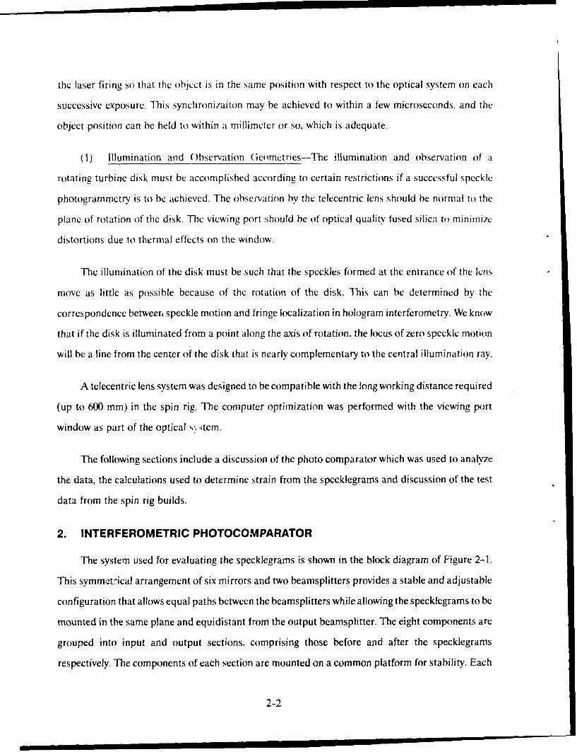
(1) Illumination and Observation GcoMettries--The illumination and observation of a

rotating turbine disk must be accomplished according to certain restrictions if a successful speckle

photogrammetry is to be achieved. The observation by the telecentric lens should be normal to the

plane of rotation of the disk. The viewing port should be of optical quality fused silica to minimize

distortions due to thermal effects on the window.

The illumination of the disk must be such that the speckles formed at the entrance of the lens

move as little as possible because of the rotation of the disk. This can be determined by the

correspondence betweer, speckle motion and fringe localization in hologram interferometry. We know

that if the disk is illuminated from a point along the axis of rotation. the focus of zero speckle motion

will be a line from the center of the disk that is nearly complementary to the central illumination ray.

A telecentric lens system was designed to be compatible with the long working distance required

(up to 600 mm) in the spin rig. The computer optimization was performed with the viewing port

window as part of the optical s; tem.

The following sections include a discussion of the photo comparator which was used to analyze

the data, the calculations used to determine strain from the specklegrams and discussion of the test

data from the spin rig builds.

2. INTERFEROMETRIC PHOTOCOMPARATOR

The system used for evaluating the specklegrams is shown in the block diagram of Figure 2-1.

This symmet"ical arrangement of six mirrors and two beamsplitters provides a stable and adjustable

configuration that allows equal paths between the beamsplitters while allowing the specklegrams to be

mounted in the same plane and equidistant from the output beamsplitter. The eight components are

grouped into input and output sections, comprising those before and after the specklegrams

respectively. The components of each section are mounted on a common platform for stability. Each

2-2

SPECKLEGRAMMOUNTMJRRL)R MUN

RMIRROR

MMRO R'DTETO

_ _ _ _ _ _ MIRROR

ETALON SPECKLEGRAM

QUARTERWAVE,-" PLATE

ROTATINGZ TRANSLATION STAGEHALFWAVE

PLATE

Figure 2-1. Protocomparator block diagram.

beamsplitter and the central mirror near it are mounted on a common translation stage for centering

adjustment. All mirrors and beamsplitters are adjustable for tilt. These adjustments make it possible

to align all beams so as to lie in a common plane.

The optics before the interferometer consist of a lens to focus the beam at the plane of the output

detectors, an etalon for translating the beam, and an arrangement for generating a Doppler shift. The

Doppler shift is generated by a rotating halfwave plate followed by a quarterwave plate set at 450 to the

vertical axis. The etalon is rotated either about a horizontal axis to translate the beam vertically or

about a vertical axis to translate it horizontally.

The specklegrarns are mounted on an X/Z translation stage to position them so that the beam

passes through the spot where a strain measurement is desired. Each mount has horizontal and

vertical translation adjustments as well as a rotation adjustment which allows a new specklegram to be

placed on it and aligned with the one on the other stage.

2-3

The output detector array consists of 24 silicon photodiodes, each with an amplifier. These are

connected to a multiplexer that connects diametral pairs to a pair of high-O filters which feed their

signals to a phase meter. The phase meter, the multiplexer, the X/Z translation stages. and the etalons

are all under computer control so that the system can operate automatically once a pair of

specklegrams have been aligned in the system.

3. MATHEMATICAL THEORY

The calculations for strain can be described from Figure 2-2. The two specklegrams appear

~F=HALO FRINGE VECTOR

L=DISPLACEMENT VECTOR

D=HALO DISTANCE FROM SPECKLEGRAM

SPECKLEGRAM

Figure 2-2. Specklegram schematic.

superposed when viewed through the output beamsplitter, except for the small displacement, L. This

displacement generates the fringes seen in the halo which may be described by the fringe vector, F,

from the center of the halo to the first bright fringe. These vectors are related by the equation

2-4

L = ,LDF, (1)

where D is the distance from the specklegram plane to the halo plane. Taking the differential of Eq. (1)

gives

AL = ADAF, (2)

If the object was strained between the two specklegram recordings, a small shift of the readout beam,

AR, will generate the differential displacement according to

AL = {f}AF, (3)

where {f} is a matrix describing the inplane strains {E} and rotations {0}, i.e.,

{f} = {E} + {0}. (4)

Combining Eqs. (2) and (3) gives

{f)AR = ADAF (5)

2-5

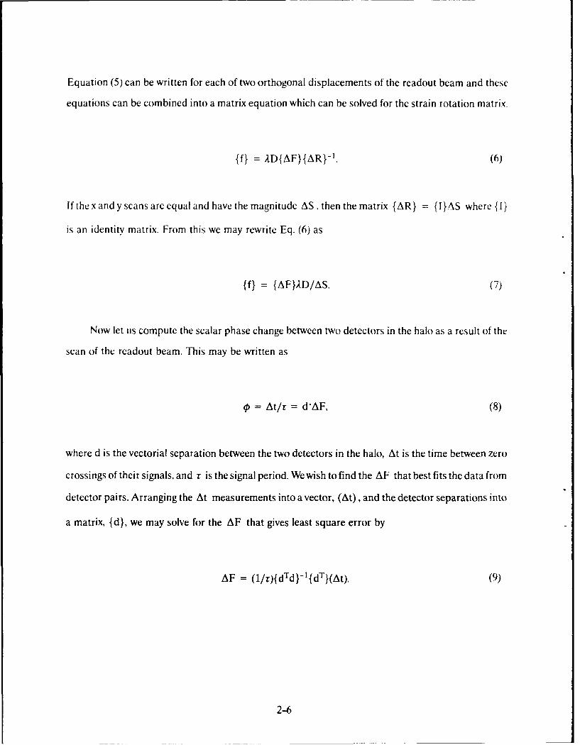
Equation (5) can be written for each of two orthogonal displacements of the readout beam and these

equations can be combined into a matrix equation which can be solved for the strain rotation matrix.

{f} = ,D{AF}{AR} - 1 (6)

If the x andy scans are equal and have the magnitude AS, then the matrix {AR} = {I}AS where {i}

is an identity matrix. From this we may rewrite Eq. (6) as

{f} = {AF}AD/AS. (7)

Now let us compute the scalar phase change between two detectors in the halo as a result of the

scan of the readout beam. This may be written as

0 = At/r = d'AF, (8)

where d is the vectorial separation between the two detectors in the halo, At is the time between zero

crossings of their signals, and r is the signal period. We wish to find the AF that best fits the data from

detector pairs. Arranging the At measurements into a vector, (At) , and the detector separations into

a matrix, {d}, we may solve for the AF that gives least square error by

AF = (1/r){d Td}-{dT}(At). (9)

2-6

Suhstititing this into Eq. (7) gives

{f} = (AD/rAS){d'd}-l{d T} {At}. (10)

This is the equation used to compute the strains and rotations from the output measurements of the

interferometer. The strains are obtained by taking the symmetrical portion of {f}, i.e.,

{E} = [{fT}]/2. (11)

4. PHOTOCOMPARATOR PROCEDURE

This is a description of the procedure followed with the photocomparator. First, the two

specklegrams to be compared were placed in their holders on the X/Z translation stage with the radial

direction vertica,. The position and angle of one was adjusted until the two images seen through the

beamsplitter merged. This was adequate to obtain halo fringes which were used to make fine

adjustments. The position and angle of one specklegram was adjusted until the fringes were as broad

as possible with the best possible contrast when the beam passed through the center of the region of

interest. A further check on the angular alignment was obtained by moving the stage so as to scan the

beam across the specklegrams. The best angular alignment was when the fringes did not rotate with the

scan.

Four points were located at the 152-mm radius and four at the 165-mm radius. The stage

coordinates that positioned these points under the readout beam were recorded, and these were stored

in the computer. The program was initialized and ran. This consisted of moving the stages to the first

point, rotating the etalon to scan the beam up, down, and back up, followed by left, right and back to

left. The total beam scan was 1.3 mm. All detector pairs were read at each of the six positions and the

2-7

data stored. Values for At were computed from the first three, and the second three values for each

detector pair by the formula

At = (At 1 + At,- 2ATz)/2, (12)

which compensated for linear drift of the readings. The two values for At obtained became elements

for the {At} matrix in the computation of Eq. (10). The strain-rotation matrix was calculated for each

point and the four points at each radius were averaged to reduce errors. The symmetrical portions of

the matrices were taken as the strains. Generally, the shear terms were negligible indicating that the

principle strain axes were radial and circumferential.

5. BUILD 1 - SPECKLE PHOTOGRAMMETRY

a. Data Recording-During Build 1 of this contract, the UTRC speckle photogrammetry

system was used to record data on the turbine disk. The system assembled at the spin rig included:

1. Q-Switched Pulsed Ruby Laser (JK Lasers, Ltd., Output of 10 J in 30 nsec)

2. Specklegram Recording System

3. Programmable Control Box for Laser Firing and Operation of the Recording

System

The laser system consisted of a laser head, cooling system, flash lamp firing electronics, and

Q-switch firing electronics. An external cooling source (in the form of an ice bath) had to be provided

to the laser cooling system because the local tap water was too warm. The specklegram recording

system consisted of a telecentric lens system with electronic shutter, a photographic plate changer, a

450 mirror to rotate the vertical lens axis 900 to the plate changer, and two high power mirrors and a

diverging lens to direct the illuminating beam to the disk. The 450 mirror mount also held an

alphanumeric display and relay lens to allow run number, plate number, and rotation speed to be

printed on each plate. This system is diagrammed in Figure 2-3.

2-8

PLATECHANGER

CONTROL _ _ MRROR

STAND

TELECENTRIC' LENS

rSPIN RIG LID

ILLUMINATIONBEAM

Figure 2-3. Optical arrangement in spin rig.

The programmable control box was interconnected with the system as indicated in Figure 2-4.

Timing pulses from the spin rig (1/rev) were received by the control box and synchronized by a

phase-lock loop so as to provide a precursor pulse to fire the flash lamps a set time before the timing

pulse. These pairs of flash lamp and timing pulses were fed through gates to the laser flash lamp firing

controls and the Q-switch firing control. (The latter had to be added to the laser control box from

information provided by tew manufacturer.) When the fire button was pushed, a command was sent to

the shutter to open it and to start a counter to measure the spin rig speed. The flash synchronization

switch on the shutter sent a signal to open the gates that inhibited the flash lamp and 0-switch signals.

This allowed the next pair of pulses to fire the laser (provided the system is in phase lock) after which

the shutter closed. The output of the laser was monitored on an oscilloscope, and, if a laser pulse had

occurred, a keyboard command continued the sequence which printed the information on the plate

and advanced the plate changer. If no pulse occurred, the system was reset and the unexposed plate

used again.

2-9

LASER FLASH PULSE

0-SWITCH PULSE

1/REV RIG PULSE SHUTTER OPEN

SHUTTERFLASH SYNC

CONTROLBOX

KEYBOARD PLATE ADVANCEPLATE

CHANGER

LABEL

Figure 2-4- Laser control schematic.

Initial exposures showed large image shifts between photographs at different specds due to a

large time delay in the signal from the spin rig. After this was eliminated, the image shift hetw'en

lowest (1621) r/min) and highest ( 13.2(X) r/min) speeds was in the order of 5 mm. which corresponds to

about 25 ,s delay. Difficulties were also experienced with the plate changer, which required

replacement of four internal springs. Difficulties were also experienced with the spin rig heaters and

with the actuator that opened the view to the heated chamber.

Data were taken at five speeds at each of four temperatures. The target speeds were:

VAX) r/min - plate 1 66lX) r/min - plate 2 9330 r/min - plate 3

1143(0 rmin - plate 4 1321X) r/min - plate 5

These were chosen to give equal increments in the square of rotation speed and thus equal increments

in stress to the disk.

2-10

6. DATA PROCESSING

The photographs were developed in HC110B Developer after which they were inspected for

image correlation After this they were converted to dichromated gelatin images for use in the

heterodyne photocomparator. Due to three errors the following data points were not obtained:

1. Ambicnt Temperature - Plates 3 and 4.

The plate changer did not advance after plate 3 was exposed. the reason for this was never

dctcrmincd, and it did not happen again.

Plates 2 and 5 were analyzed and provided data that bridged this gap.

I 589 K - Plate 1.

Plate I was missed when the plate transport was unloaded for development. Plate 2 at ambient

temperature \kas compared with plate 2 at 589 K to provide a reference for the 589 K run. Isotropic

expansion due to the temperature change was subtracted from the resultant data.

3. 589 K - Plate 3.

Plate 3 was loaded into its holder glass side out and exposed backwards. Plates 2 and 4 were

analyzed to bridge this gap.

The actual speeds at which useable data were recorded are tabulated below in Table 1.

TABLE I. SPEEDS AND TEMPERATURES AT WHICH DATA WERE TAKEN

300 K 422 K 589 K 755 K

1. 1680 1630 1590

2. 6870 6770 6610 6550

3. 9420 9250

4. 11,490 11,340 11,320

5. 13,480 13,320 13,110 13,170

2-11

Eight points were located on a spare photograph, points 1 - 4 at a radius of 165 mm from the

center of the disk and points 5 - 8 at a radius of 152 mm. This plate was placed in the comparator and

the stages moved until the readout beam passed through each point.

This allowed the desired stage positions to be entered into the computer. The plate was also used

as a reference to assure that the plates from each data run were evaluated at the same locations.

Pairs of data plates were placed in the photocomparator and aligned, after which they were

processed for differential strain. The strain results for each location were printed and stored in the

computer. The results for points 1 -4(165 mm radius) were averaged as were the results for points 5 - 8

(152mm radius). The averages are plotted versus the square of rotation speed tr/min] 2 in Figures 2-5.

300 K8K

6K

Z

u) 4K0_Cn- 152 mm --" 5Rn K -

2K152 mm C

0 _j0 50K lOOK 150K

ROTATION SPEED SQUARED (RPM) 2

Figure 2-5. Build 1 strain vs. speed squared, 300 K.

2-6, 2-7, and 2-8 corresponding to temperatures ot 300 K, 422 K, 589 K, and 755 K respectively. The

curves plotted are labeled according to radius (165 mm or 152 mm) and strain orientation (R = radial

and C = circumferential).

2-12

422 K8K

6K

S4K0(r

2K

00 50K I OOK 150K

ROTATION SPEED SQUARED (RPM) 2

Figure 2-6. Build 1 strain vs. speed squared, 422 K.

589 K8K-

6K

U4K0C-)

2K -12m

00 50K 100K 150K

ROTATION SPEED SQUARED (RPM) 2

Figure 2-7. Build I strain vs. speed squared, 589 K.

2-13

755 K8K

6K - 152 mmnR -

Cn 4K

0

2K

00 50K 100K 150K

ROTATION SPEED SQUARED (RPM) 2

Figure 2-8. Build I strain vs. speed squared, 755 K.

7. DISCUSSION

The results plotted in Figures 2-5 through 2-8 show excessively large values for the radial strains.

particularly at the three elevated temperatures. The peak strains measured would correspond to

values of stress greater than 1380 MNm -2 , which should cause the disk to yield. Also, the slopes of the

radial strain plots decrease as the square of speed increases. This appears to indicate the presence of

an apparent radial strain that is directly proportional to speed and not related to stress. To estimate

the magnitude of this apparent strain, the data at each temperature were fit to the following function:

Strain = A [speed] + B jspeedl 2, (13)

where A and B are coefficients determined by a least-square-error fit. The average value of the linear

component of radial strain is approximately 4.1x10 -3 .

2-14

The only thing within the entire setup that varies linearly with speed is the angular position of the

disk. This was measured to be about 30 mrad between low speed and full speed. It is generated by the

25 pis delay between the once-per-revolution pulse of the rig and the laser light pulse. If the object

surface were exactly focused on the photographic plate, this translation and rotation would have no

effect on the process because speckles observed on the surface of the object cannot move relative to

that surface. Speckles observed above or below the object surface may exhibit slewing due to tilts of the

object surface, but this effect is generally a uniform speckle translation that does not generate

apparent strain.

The primary source of apparent strain comes from a linear variation of defocusing, i.e. an

inclination of the object surface to the focal plane. This causes admixture of the observed strains with

surface rotations and also a variation of speckle slewing across the focal planie The surface of the disk

was profiled to determine its variations in height as a function radius. The slope in the radial direction

was found to be 0.066 at 152 mm in and 0.037 at 165 mm.

Further analysis of the particular geometry used in the spin rig tests, i.e. illumination from a point

source located on the axis of rotation, showed that this eliminates apparent strain due to angular

rotation of the disk. The simple explanation for this is that the curvature of the illuminating wavefront

is matched to the curved track of any point on the disk. The angular rotation of the disk does not cause

it to move relative to the apparent illumination, and, therefore, the speckles cannot move relative to the

disk itself, regardless of defocusing. Even if this were not the case, however, the very small slope of the

disk surface would not allow apparent strains large enough to account for the observations.

Another source of apparent strain could come from distortions of the mirror that rotates the

optical axis by 900. For example, cylindrical bending of the mirror would cause the image to be

magnified differently along one axis than at right angles to that axis. This can cause angular rotations

to appear as apparent strains according to the formula,

2-15

cap = 0,(m 2 - 1)/2m (14)

where t ap is the apparent strain, 0, is the angular rotation, and m is the unidirectional magnification.

To convert 30 mrad into 4.1 millistrain would require a unidirectional magnification of 1.075. This

would be observable by the naked eye when looking through the mirror.

Nonetheless, tests were performed to check for such effects. The lens and mirror were mounted

on the optics table in the laboratory, and an object was constructed that could be made to pivot about

an axis simulating that of the disk in the spin rig. Specklegrams were recorded before and after

rotations of 30 mrad and 15 mrad. Analysis of these pairs of specklegrams showed that some apparent

strain was caused by the mirror, but that its pattern was geometrically random and its magnitude was

in the order of 500 to 600 microstrain. We must conclude that the mirror distortions present are

insufficient to cause the apparent errors that were observed.

Finally, additional tests were performed to confirm the correct operation of the interferometric

photocomparator. First, the photocomparator was run with a pair of calibrated, unidirectional strain

specklegrams, and these confirmed the correct operation of the comparator. Second, the

specklegrams from the spin rig were evaluated on the comparator in a manual mode. Pairs of plates

were aligned on the comparator, the stage that moves the pair of plates was incremented by 10 mm, and

the amount of displacement of one specklegram required to rezero the halo fringes was measured and

divided by 10 mm. The effective gage length by this method becomes 10 mm in contrast to 1 mm by the

automated method. This was done for plates 1 and 2, and for plates 2 and 5 for each run, and the

results are plotted in Figure 2-9, together with averaged results from the automated analysis. The

strains measured manually uniformly exceed those measured by the automated method. This makes it

difficult to disprove the photocomparator measurements.

8. CONCLUSIONS ANt) RECOMMENDATIONS FROM BUILD 1

The speckle photogrammetry measured strains on the spinning disk. These measurements had

an excessively large component of radial strain for which no error source could be identified. The 450

2-16

t ,TRA • c A

1-0e

qo.SGAGF

F SPFEO,F . . . .E D

Figure 2-9. Build I effect of gage length on measured strain for varioustemperatures.

mirror was designated to be replaced with a thicker and flatter one to improve system accuracy, and

further tests were scheduled for the next build to help identify sources of error. Such tests were to

include the following:

1. Specklegrams would be recorded during the next build for both accelerating and decelerating

rig speeds. This would check for some time varying effects such as laser heating and heat propa-

gation through the disk.

2. Two sets of specklegrams would be recorded at room temperature on the disk, one with the rig

rotating in one direction and the other with it rotating in the other direction. If a speed related

apparent strain is present, its sign would reverse with reversal of the rotation direction. Even

if the mechanism could not be determined, the effect could be numerically removed from the

data by this test.

2-17

9. ADVANCED STRUCTURAL INSTRUMENTATION BUILD 2 - SPECKLEPHOTOGRAMMETRY

a. Data Recording--The specklegram recording equipment was set up at the spin rig as in

Build 1 with the following changes:

1. The circuitry used to provide pulses to fire the flash lamps and Pockels cell of the

laser was rebuilt to utilize digital logic circuitry in place of the phase-locked loop

used in Build 1. This provided more noise resistance and allowed operation over

a wider range of rig rotation speeds.

2. The 450 mirror used to reflect the image to the plate holder was replaced with a

thicker mirror of more accurate figure, and it was mounted so that no bending

stresses were applied.

3. A new high-speed detector was designed to provide the 1/revolution pulse from the

spin rig. This provided less time delay than the previous circuitry and reduced the

angular rotation of the image between minimum and maximum speeds to about 2.5

mm which is half the amount observed in Build 1.

The same target speeds were used as in Build 1 except for the lowest speed which was 1200 rpm.

The target speeds and temperatures are tabulated below.

Target Speeds Target Temperatures

1200 rpm ambient

6600 rpm 422 K

9330 rpm 589 K

11,430 rpm 755 K

13.200 rpm 950 K

Except for the ambient temperature runs, ten specklegrams were recorded at each temperature

rin, five as the speed was increased, and five as it was decreased. At ambient temperature, five

2-18

specklegrams were recorded while the speed was increasing, however, data were taken for both

clockwise and counterclockwise rotations. Data were recorded successfully at all speeds and at all

temperaturcs except for the speed of 9330 rpm at ambient temperature with counterclockwise

rotation. All of the high temperature data were taken with the rig running in the counterclockwise

direction.

10. DATA PROCE3SING

The specklegrams were developed and bleached to colloidal silver for processing in the

hetcrodvne photocomparator. The quality of the data was generally very good and the strain results

obtained during this build are those in which the most confidence is placed with regard to the

technique of speckle photogrammetry. The image magnifications measured by the heterodyne

photocomparator were first corrected by subtracting a systematic error in the comparator measured

by analyzing a pair of identical specklegrams. When comparing specklegrams at high temperatures,

thermal expansions were estimated from thermocouple measurements and subtracted. A correction

was also made to the resulting data based upon measurements of the slope of the surface of the disk

and of measurements of surface tilt as a function of speed. The tilt creates an apparent enlargement of

the disk in the radial direction. These corrections amounted to the following:

Speed 165-mm radius 152-mm radius

(r/min) p. Strain . Strain

6600 124 221

9330 75 140

11,430 53 101

13,200 33 66

An additional fea" ire was obtainable with this set of data. Comparisons could be made between the

low speed specklegrams at neighboring temperatures, and these made it possible to define the initial

strain state of the disk at each new temperature by subtracting the thermal expansion. The strain

measurements are tabulated as follows:

2-19

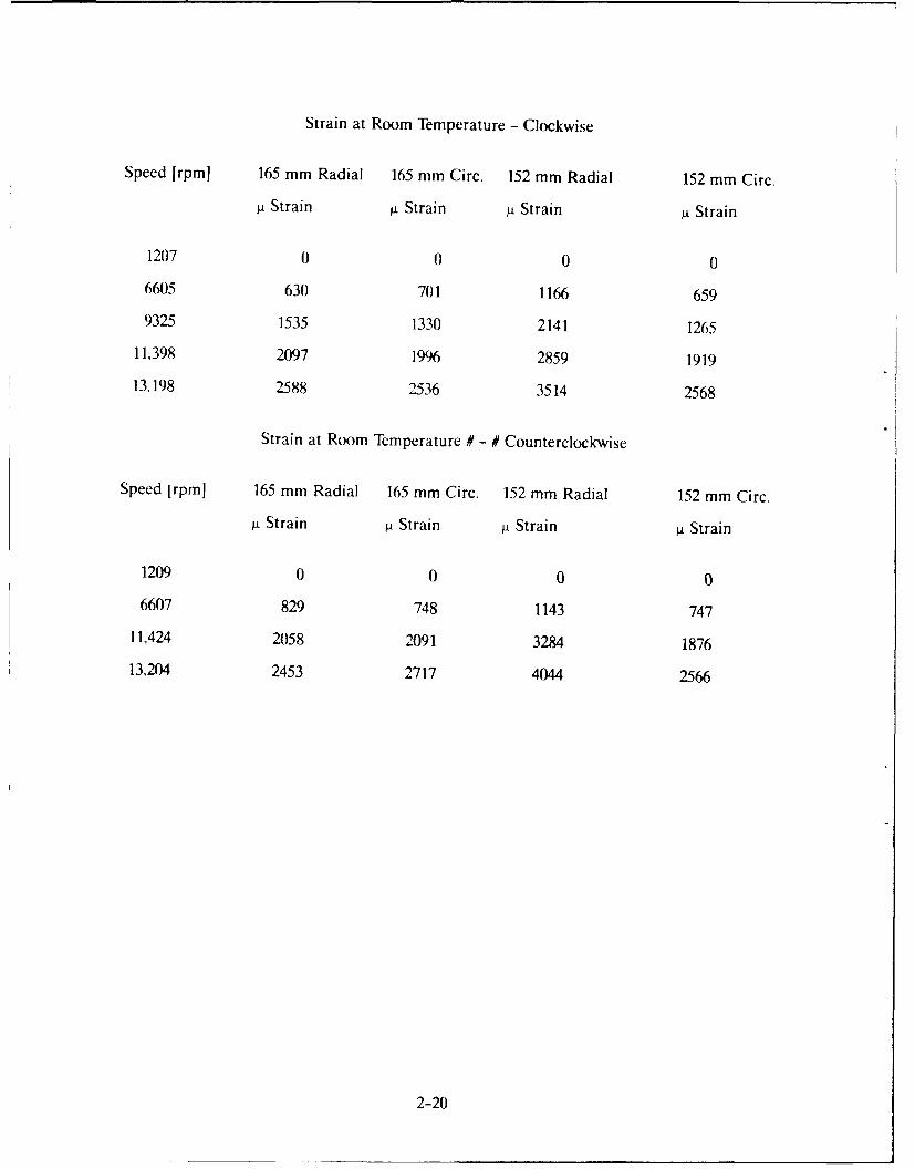
Strain at Room Temperature - Clockwise

Speed [rpmJ 165 mm Radial 165 mm Circ. 152 mm Radial 152 mm Circ.

A. Strain i Strain g Strain 4 Strain

1207 0 0 0 0

6605 630 701 1166 659

9325 1535 1330 2141 1265

11,398 2097 1996 2859 1919

13,198 2588 2536 3514 2568

Strain at Room Temperature # - # Counterclockwise

Speed [rpm] 165 mm Radial 165 mm Circ. 152 mm Radial 152 mm Circ.

A± Strain g Strain gi Strain . Strain

1209 0 0 0 0

6607 829 748 1143 747

11,424 2058 2091 3284 1876

13,204 2453 2717 4044 2566

2-20

Strain at 422 K

Speed [rpm] 165 mm Radial 165 mm Circ. 152 mm Radial 152 mm Circ.

ji Strain g Strain gi Strain g Strain

1207 733 -347 627 -483

6603 19(y) 315 1940 241

9345 2575 1200 3028 1063

11,415 3681 1764 4447 1578

13,215 4X)8 2565 4968 2295

13.210 4054 2586 4960 2336

11.402 3430 2018 4194 1677

9334 2800 1450 3338 1138

6613 1730 812 2191 498

1203 362 92 465 -92

Strain at 589 K

Speed [rpm] 165 mm Radial 165 mm Circ. 152 mm Radial 152 mm Circ.

i Strain p Strain p Strain g Strain

1209 1626 -854 1566 -1197

6609 2727 177 3063 -181

9296 3643 1106 4078 710

11,398 4151 1714 4771 1524

13,204 4949 2384 5711 2133

13,204 4950 2409 5769 2297

11,398 4337 1837 4932 1781

9331 3431 1334 3944 1234

6605 2477 607 2779 530

1206 1279 -33 1065 96

2-21

Strain at 755 K

Speed [rpm] 165 mm Radial 165 mm Circ. 152 mm Radial 152 mm Circ.

g Strain gi Strain g. Strain g. Strain

1197 2433 -405 2627 -685

6609 3600 270 3955 39

9319 4304 1104 5044 746

11,424 5256 1901 6134 1555

13,140 5824 2815 7051 2460

13,204 5774 2797 7032 2296

11,415 5057 2064 5971 1642

9337 4501 1314 5213 852

6603 3484 666 3766 301

1219 2099 -277 2088 -544

Strain at 950 K

Speed [rpm] 165 mm Radial 165 mm Circ. 152 mm Radial 152 mm Circ.

ji Strain A Strain A. Strain A. Strain

1197 2083 -878 1776 -938

6609 3950 -75 4092 -108

9319 5083 689 5479 630

11,424 5822 1428 6544 1601

13,140 6839 2478 7788 2553

13,204 6337 2250 7324 2260

11,415 6057 1372 6742 1519

9337 5327 692 5752 833

6603 4430 -115 4506 68

1219 1637 -1084 1714 -672

2-22

These data are also plotted in Figures 2-10 through 2-15 with solid lines indicating the data for

increasing speeds and dotted lines indicating the data for decreasing speeds.

Comparisons were made between the first and last photographs in each of the high temperature

runs. These provided an indication of the cumulative error encountered in the processing of the ten

plates in sequence and also confirmed the change in strain state of the disk over the time period of the

test. The following is a tabulation of these data together with the data from analysis of the sequence of

ten plates.

422 K

location/ 10-1 direct 10-1 sequential direction

g Strain t Strain

165 mm radial -261 -371

165 mm circum. 446 439

152 mm radial -159 -162

152 mm circum. 494 391

589 K

location/ 10-1 direct 10-1 sequential direction

pi Strain . Strain

165 mm radial -520 -347

165 mm circum. 996 821

152 mm radial -20 -501

152 mm circum. 1127 1293

2-23

755 K

location/ 10-1 direct 10-1 sequential direction

4 Strain j Strain

165 mm radial -265 -334

165 mm circum. 414 128

152 mm radial -275 -530

152 mm circum. 444 141

950 K

location/ 10-1 direct 10-1 sequential direction

pi Strain 4 Strain

165 mm radial -261 -446

165 mm circum. 216 -206

152 mm radial -279 -62

152 mm circum. 375 266

11. DISCUSSION

The plots of strain versus speed (Figs. 2-10- 2-15) are much more linear in this build than in the

previous one. This is due in part to the correction for surface tilting of the disk with increasing speed. It

is assumed that the disk flexes so that the rim bends upward relative to the hub. It was also significant

that very little difference was detected in the strains measured with the disk rotating in the clockwise

and counterclockwise directions. This supports the conclusion that the strains measured here are very

likely accurate to within a few hundred microstrain,

2-24

8000 c, 165 mm RADIUS, RADIAL

c 165 mm RADIUS, CIRCUMFERENTIAL

7000 r- 152 mm RADIUS, RADIAL

x 152 mm RADIUS, CIRCUMFERENTIAL6000

z< 5000

U)o 4000

0 3000

2000

1000

0

-1000 25 50 75 100 125 150 175

SPEED SQUARED (RPM) 2x10 6

Figure 2-10. Build 2, strain vs. speed squared. Ambient temperature, clockwiserotation.

8000 o 165 mm RADIUS, RADIAL

o .65 mm RADIUS, CIRCUMFERENTIAL7000 - C 152 mm RADIUS, RADIAL

6000 - 152 mm RADIUS, CIRCUMFERENTIAL

z 5000

r 4000V)0r 3000

2000

1000

0

-1000 25 50 75 100 125 150 175

SPEED SQUARED (RPM) 2xl06

Figure 2-11. Build 2, strain vs. speed squared. Ambient temperature,counterclockwise rotation.

2-25

8()00 16 1 mm RADIS RADIAL7000

5~ Mm R DIUS,

INCJ*** .D C R EASIN G SP E15 mRADIUS,

M'C&FERAT4 ........

6000 12 mm RDIUS, 4DI4L ... DCREASIN PE

600 l~ mm ILsCIRCUMFE ENTA

0

-1 000

80 00 0 256 m R DI S R DA70005

75 10mm

U0CRC

80( 0 6 5 mmp~~ RADALIRUNS,

1 5 2. . . . . . . . . . . . . .. . . ..IN R A I6000 DECREASIN 0 SPEED

600 ~ S~ m R DIS' CIRCUJMFERENTA

Z 4000

4000

0. . .. . . . ...: t : : ~ ................ .... ..... ... .......... ...u......u......

1000

SPEED SQUARED (R PM125. 15017

Figu ~~ro aton

253B il qu r s 9 K tern perature

8000 0 165 mm RADIUS, RADIAL INCREASING SPEED0 165 mm RADIUS, CIRCUMFERANTIAL ................... DECREASING SPEED

7000 0 152 mm RADIUS, RADIALX 152 mm RADIUS, CIRCUMFERENTIAL

6000

2 5000

1- 4000

0

1000

2 0 0 0 .. .. ..................

0 [ .. .... .............

-1000 _ 25 50 75 100 125 150 175

.SPEED SQUARED (RPM)2x1 06

Figure 2-14. Build 2, strain vs. speed squared. 755 K temperature,counterclockwise rotation.

8000 0- 165 mm RADIUS. RADIAL INCREASING SPEED0 165 mm RADIUS, CIRCUMFERENTIAL .......... DECREASING SPEED ....I

7000 - 0 152 mm RADIUS, RADIAL ...... ...........

X 152 mm RADIUS, CIRCUMFERENTIAL ................

6000 - .........

5000 -zn- 400016--C,)0 3000

n-o

10000 A ........

........ ..-

''

-1000 . 25 50 75 100 125 175

SPEED SQUARED (RPM)2x104

Figure 2-15. Build 2, strain vs. speed squared. 950 K temperature,counterclockwise rotation.

2-27

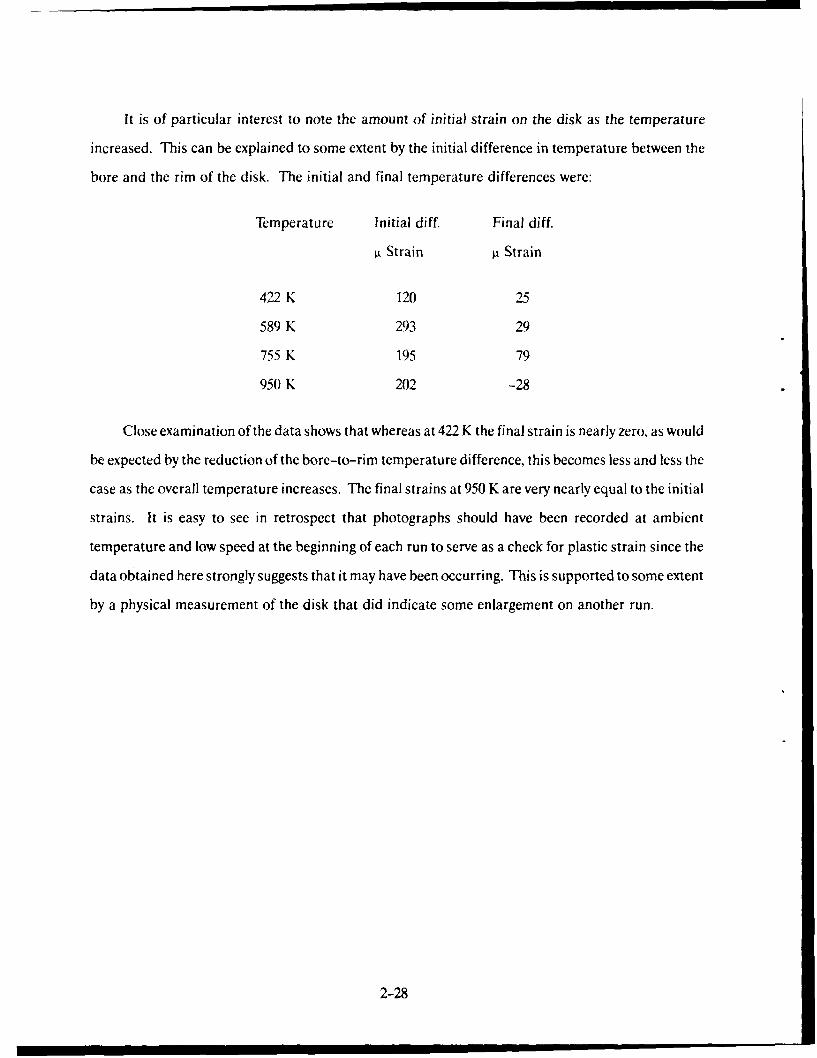
It is of particular interest to note the amount of initial strain on the disk as the temperature

increased. This can be explained to some extent by the initial difference in temperature between the

bore and the rim of the disk. The initial and final temperature differences were:

Temperature Initial diff. Final diff.

Strain i Strain

422 K 120 25

589 K 293 29

755 K 195 79

950 K 202 -28

Close examination of the data shows that whereas at 422 K the final strain is nearly zero, as would

be expected by the reduction of the bore-to-rim temperature difference, this becomes less and less the

case as the overall temperature increases. The final strains at 950 K are very nearly equal to the initial

strains. It is easy to see in retrospect that photographs should have been recorded at ambient

temperature and low speed at the beginning of each run to serve as a check for plastic strain since the

data obtained here strongly suggests that it may have been occurring. This is supported to some extent

by a physical measurement of the disk that did indicate some enlargement on another run.

2-28

II. HEAT FLUX SENSORS

1. SUMMARY

Under the Advanced Structural Instrumentation program, heat flux sensors were fabricated into

turbine blades and tested under rotation in a spin pit rig. The heat flux sensors were constructed into

blade halves which were later joined by brazing. After assembly, the blades underwent final machining

to demonstrate the feasibility of machining the blades with small diameter lead wires installed. The

heat flux sensors were then calibrated using a quartz lamp bank as a heat source. During Build 2 of the

ASI rig, the blades were installed on a disk and then mounted in the spin rig. A slip ring assembly was

used to route the sensor leads out of the rig. Although there was minimal heat flux and no coolant flow

through the blades, the heat flux sensor outputs and blade temperatures were monitored during the

rotational testing. One sensor failed early in the test program and the thermocouple in that sensor

functioned intermittently. Post-test analyses showed all sensor failures were in the external lead wires,

indicating that the heat flux sensor fabrication technique produces sensors capable of withstanding

the centrifugal forces created by rotation. Based on the test results, recommendations for improved

techniques for handling the external lead wires were generated.

2. INTRODUCTION

Designing durable turbine airfoils, which use a minimum amount of cooling air (and are,

therefore, more efficient and economical), requires detailed knowledge of heat flux characteristics

within the hot section of advanced aircraft gas turbine engines. Considerable development has been

done on both low and high temperature heat flux sensors for such diverse purposes as basic boundary

layer experiments, solar power and energy conservation investigations, research on thermal protection

systems for advanced aircraft and spacecraft, and application in advanced aircraft combustors. None

of those applications combines the requirement for materials compatibility, miniaturization, and

survivability in a hostile environment that is necessary for a viable turbine airfoil heat flux sensor. Due

to the inherent limitations of current sensors, it has been impossible to collect hard empirical data

relating to the heat transfer taking place in operating turbine airfoils in aircraft gas turbine engines.

As an undesirable alternative, investigators have been forced to rely on heat flux predictions derived

3-1

from ad hoc analytical models. These models are themselves unverifiable due to the very lack of

empirical data they seek to remedy.

From this standpoint, the importance of accurate and durable heat flux sensors in the

development of advanced gas turbine engines becomes apparent. The development of these sensors

would provide a diagnostic tool enabling the verification or modification of analytical procedures used

to design improved durability and longer life turbine airfoils. These, in turn, would promote a hnger

component life while minimizing the amount of cooling required, thus advancing fuel efficiency and

maintenance economy.

To address the requirement for heat flux sensors suitable for use on turbine airfoils, a

development effort was initiated at Pratt & Whitney under the NASA Hot Section Technology (HOST)

(Refs. 1 and 2) program. Tests of the resulting sensors in a full scale rotating rig under the ASI program

were a continuation of that development effort.

3. DESCRIPTION OF SENSORS

For gas turbine applications, heat flux measurements are required under steady state as well as

transient conditions. For that reason, development was concentrated on sensors, capable of making

both types of heat flux measurements.

Two types of heat flux sensors were chosen for fabrication into the blades used in the ASI

program. These were an embedded thermocouple sensor and a Gardon gauge sensor.

Embedded thermocouple heat flux sensors determine heat flux by measuring the differential

thermoelectric output from Alumel wires in the hot and cold side of the airfoil wall. This output is the

result of the thermal drop across the wall generated by the transmitted heat flux.

Embedded thermocouple sensors require installation of lead wires in both the hot and cold side

of the airfoil wall. In order to maximize thermocouple wire size to increase durability while keeping the

required slots in the airfoil wall small, these sensors were designed with three single conductor swaged

wires. Figure 3-1 illustrates the design for the embedded thermocouple sensor. In this design, both an

3-2

ELECTRICAL SCHEMATIC EMBEDDEDEMBEDDED SWAGED WIRE THERMOCOUPLES THERMOCOUPLE SENSOR

CHROMEL ALUMEL ALUMELCOLD SIDEA \ E -, -/ ALME

CHROMEL

900 //COLD SIDE 2

AIRFOIL WALL

HOT SIDE \ _ ALUMEL

ALUM EL- 3AIRFOIL WALL

1-3 =SENSOR OUTPUT

HOT SIDE A 1-2 =REFERENCE TEMPERATURE

Figure 3-1. Schematic of the embedded thermocouple heat flux sensor.

Alumel and Chromel wire were embedded in the cold side of the blade and an Alumel wire was

embedded on the hot side. The sensor output was obtained as a differential signal from the Alumel

wires. The Chromel/Alumel thermocouple yielded a reference temperature.

The Gardon gauge sensors also depend on a thermal differential generated by heat flow in the

airfoil wall. For these sensors the heat flow is in a radial direction through a thin disk of airfoil material

on the hot side of the airfoil wall.

Gardon gauge sensors require installation of lead wires on only the cold side of the airfoil. In

order to minimize machining, these sensors were designed with a single sheathed three-conductor

cable. Figure 3-2 shows a schematic for the Gardon gauge sensor. For this design, two Alumel wires

and one Chromel wire were installed in a single sheath that was embedded in the cold side surface.

This unique three-conductor cable was produced to our specifications by Idaho Labs (Ref. 3). The

cavity required to form the Gardon gauge foil was formed by electro-machining the cold side of the

airfoil wall. One Alumel lead was attached to the bottom center of the cavity; the other Alumel lead and

3-3

GARDON GAUGE ELECTRICAL SCHEMATIC GARDONGAUGE SENSOR

CERAMIC AUEINSULATING COLD SIDE ALUMELMATERIAL 2 2(FILL) ICHROMEL

COLD SIDE 3

AIRFOIL WALL

ALUMELCHROMEL HOT SIDE

AIRFOIL WALL 1-2 =SENSOR OUTPUT

HOT SIDE 1-3 = REFERENCE TEMPERATURE

Figure 3-2. Schematic of the Gardon gauge heat flux sensor.

the Chromel lead were attached to the wall of the cavity near the bottom. Sensor output was obtained

from the two Alumel wires, while a reference temperature was obtained from the Chromel and Alumel

wires attached to the wall. The cavity made for the Gardon gauge was filled with a ceramic cement

which provided aerodynamic integrity on the cold side as well as support and oxidation protection for

the fine thermocouple wires.

4. FABRICATION OF SENSORS INTO THE BLADES

The embedded thermocouple sensor was formed by machining a groove into the hot side wall and

two grooves into the cold side wall to accept the thermocouple wires. The grooves were cut by electrical

discharge machining and were 0.3 mm wide and 0.3 mm deep. At the thermocouple junction end of the

groove, the depth was reduced to 0.13 mm to keep the thermocouple junction as close to the surface as

possible. The thermocouple junctions were directly opposite each other on the airfoil wall, and the

grooves were approximately 900 apart to reduce the structural impact on the airfoil. The lead wires

were routed in a serpentine pattern to accommodate the centrifugal loading on the wires. The

3-4

thermocouple wire used was 0.25 mm diameter single-conductor swaged Chromel and Alumel wire.

The swaged thermocouple wires were installed in the grooves and held in place by fillet wires of

Chromel P which were resistance welded in place. After the thermoelectric ,urc!Vns were made by

resistance welding, the area around the thermocouple junction was filled with powdered MgO

insulation material to protect the thermoelectric junctions. A Hastelloy-X cap was welded over the

sensing area, and the entire groove filled with Chromel P fillet wire. After the wires were installed, the

area was smoothed by hand to restore aerodynamic integrity.

The Gardon gauge sensor was fabricated by machining a cavity 1.5 mm in diameter into the cold

side surface to a depth that left a sensor foil of the desired thickness at the bottom of the cavity. A

groove 0.55 mm wide and 0.55 mm deep was machined into the cold side wall for the lead wire. A

serpentine pattern was used to route the lead wire in order to accommodate thc centrifugal loading on

the wire. The wire used to fabricate these sensors was a three-conductor swaged wire 0.5 mm in

diameter with two Alumel and one Chromei conductor. The thermocouple wire was installed in the

channel utilizing the technique discussed above using Chromel P as a fillet wire. One Alumel wire was

attached by resistance welding in the center at the bottom of the cavity. The other Alumel wire was

attached to the sidewall of the cavity at the bottom and was oriented in the direction where the

minimum temperature gradient was anticipated. The Chromel wire was attached to the sidewall of the

cavity directly opposite the Alumel wire and was also located near the bottom of the cavity. After the

thermocouple junctions were made, the cavity was filled with M-Bond GA100 (Ref. 4) ceramic

cement. This cement provided both structural support and oxidation protection for the small wires.

After the ceramic was given an oven cure, the surface was smoothed by hand to restore aerodynamic

integrity.

The heat flux sensors were installed into two-piece blades The use of two-piece blades a!lowed

installation of the sensors prior to assembling the blades. The normal method of joining blade halves is

to use transient liquid phase (TLP)yI) bonding. A previous study by Pratt & Whitney indicated that the

thermocouple installations would not survive the TLP bond cycle of 20 hours at 1475 K. The

experimental instrumented blades did not require a long, low cycle fatigue life for this program.

Therefore, an alternate method using a 1200 K braze was used to join the blade halves. After brazing

3-5

the blade halves together, the blades were sent to a vendor for final machining of the blade attachmeijt

area below the platform. The lead wires were coiled in a 150-mm-diameter loop, and attached loosely

to the airfoil so that they could be moved easily when fixturing the blade for machining Four hladeq

were instrumented. Two blades had the lead wires damaged during machining by excessive flexing

where the lead wires exited the blade. This failure rate during machining could be reduced in the

future by the construction of rigid supports for the lead wires to prevent flexure at the point of exit from

the blade.

5. CALIBRATION

After fabrication, a program was undertaken to provide calibrations of the heat flux sensors to

determine the output versus transmitted heat flux relationship. A quartz lamp bank test facility was

used for all testing, and the blades were cooled with internal cooling air. The heat source used was a

quartz lamp bank with six parallel quartz halogen bulbs, each rated at 6 kW The bulbs are 25.4 cm

long, and the width of the lamp assembly is 7.6 cm. This lamp assembly is capable of producing a

maximum heat flux incident on the sensors of 1.7 MW/M 2. During routine operation, the lamp

operation is limited to approximately 1.0 MW/M 2 to maximize lamp life.

A photograph of the lamp face is shown in Figure 3-3. The reflector on the lamp is water-cooled,

and the bulbs are air-cooled to permit continuous operation. The airfoil under test is positioned below

the lamp and is surrounded with polished, water-cooled shields to concentrate the energy onto the

airfoil. This shielding arrangement is shown in Figures 3-4 and 3-5. The airfoil is positioned so that

the surface of the sensor area is parallel to the plane of the lamps and as close to the lamps as possible.

The polished shields are adjustable to accommodate various airfoil orientations. The heat flux output

of the lamp is monitored by a reference heat flux sensor mounted in the shield. After the shields are

positioned for a particular airfoil orientation, the airfoil is removed from the lamp assembly and a

second reference sensor is mounted at the location to be occupied by the airfoil sensor. A calibration

of the assembly is then performed to determine the relationship between the heat flux incident at the

blade location to that at the reference sensor location. This relationship is used to correct the data

measured by the reference sensor during the blade calibration. The position of the two reference

3-6

Figure 3-3. High intensity quartz lamp bank.

Figure 3-4. Airfoil positioned in quartz lamp rig with water-cooled shields -bottom view.

3-7

Figure 3-5. Airfoil positioned in quartz lamp rig with water-cooled shields - sideview.

sensors is exchanged, and the calibration is repeated to minimize the eftect of any bia in the reference

sensor calibrations on the blade calibration result. An overall view of the rig is shown in Figure >-6.

The calibrations were conducted under' ) sets of conditions: varying incident heat load at a

conmtant scnsoi temperature, and varying incident heat load at constant blade coolant flow. The heat

flux transmitted through the airfOil wall was calculated by determining the heat absorbed and

,,ubtracting the heat losses from the front face of the sensor due to convection and reradiation. The

absorbcd heat flux is equal to the incident heat flux as measured by the reference sensor, corrected to

the test sensor location, time, the emittance of the airfoil surface. Zynolyte (Ref. 5) 8M K "FHi-Temp"

paint was used to coat the blade in order to provide a constant known emittancc tf 0.89 for calibration.

The convcctive loss is equal to the concctitn heat transfer coefficient as previously measured with a

cOMcCtivC probe times the temperature differential between the sensor surface and the ambient air

temperature. "lhe rcradiation loss the cmittance of the sensor face times the difference in the fourth

Am

Figure 3-6. High intensity quartz lamp rig.

powers of the sensor surface temperature and the sink temperature. The sink temperature was

experimentally determined as approximately 400 K for this calculation.

The results of a typical sensor calibration are shown in Figure 3-7.

6. TEST RESULTS

During the ASI program, the sensors were tested to rotating speeds in excess of 13,000 r/min and

to disk temperatures above 950 K. Since the airfoils themselves were not directly heated but depended

on conduction of heat from the disk, sensor temperatures were limited to approximately 700 K. The

temperatures measured by the thermocouples in the two sensors are shown in Figure 3-8. One sensor

failed early in the test program. The thermocouple associated with that sensor became erratic and

would read correctly a portion of the time and read near room temperature the rest of the time. The

problem clearly is a., intermittent short circuit in a low temperature area. This was confirmed during

post-test inspection when significant damage was discovered in the cool lead wire area of the rig. The

other sensor and thermocouple functioned well throughout the test program.

Post-test analysis of the data showed that during those periods of time when both thermocouples

were functioning properly, there was good agreement between the two temperature measurements. No

measurable DC output was obtained from the heat flux sensor. This was as expected since there was

no heat flux through the blades. These results confirmed that neither the heating or rotation

introduced a zero offset to the heat flux sensor output.

To evaluate the AC noise level on the heat flux sensor output, several measurements were taken at

each data point, and the standard deviation of those measurements was calculated. These results are

shown in Figure 3-9. There is a low noise level (1 sigma) of about ± 0.5 counts. Some of the data,

however, shows much higher noise levels. It was eventually determined that all these data were

inadvertently recorded with power on to the inductive heater used to heat the turbine disk. When the

data with the heater on was eliminated, there were no noise signals on either the heat flux sensor or the

thermocouple that were measurable above the slip ring noise measurement.

3-10

1200 --o - a -

S

-- o ,, --0

- .. -c ,-a- 80 - / ." o-- , '-

0 . .. / . 01

z 400 - " *

-" *- , <0 Tre < 870Ka-" / . a, 1Q "re > 870K

0 25 50

HEAT FLUX TRANSMITTED, MW/mn2

Figure 3-7. Calibration data for embedded thermocouple sensor.

700 I

!0 4

TEMPERATURE BLADE1

y TEMPERATURE BLADE 2

'I

u.J

300

0 200 400 600

SEQUENTIAL POINT NUMBER

Figure 3-8. Data from two sensors from the advanced structural instrumentation

spin test.

3-11

Post-test inspection showed that for the leads that failed, all lead failures were either at the airfoil

exit (Fig. 3-10) or external to the airfoil (Fig. 3-11).

7. CONCLUSIONS AND RECOMMENDATIONS

Techniques for installation of heat flux sensors into turbine blades have been demonstrated.

The feasibility of final machining the blade root area after installation of the sensors was proven.

In the future, rigid fixturing to support the lead wires at the exit from the blade is recommended to

reduce the failure rate.

Tests in a realistic rotating environment have shown that the sensors will survive and that the

noise levels itroduced by rotation are negligible.

Application of these sensors in the rotating components of an engine should be considered.

The ASI rig has proved to be a valuable tool for instrumentation development as an intermediate

step between laboratory development nd full scale engine tests.

8 REFERENCES

1. Atkinson, W H., Cyr, M. A. and Strange, R. R., Turbine Blade and Vane Heat Flux Sensor Devel-

opment; Phase I - Final Report, NASA Contractor Report CR-168297, August 1984.

2. Atkinson, W H., Cyr, M. A. and Strange, R. R., Turbine Blade and Vane Heat Flux Sensor Devel-

opment Phase 1I - Final Report, NASA Contractor Report CR-174995, October 1985.

3. Idaho Laboratories Corporation; 2101 Hemmert Avenue; Idaho Falls, Idaho; 83401.

4. Measurements Group Inc.- P 0. Box 27777; Raleigh, North Carolina: 27611.

5. Zynolyte Products Company, Compton, California; 90220.

3-12

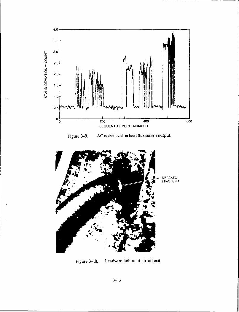
4.0

3.5-

I- 3.0z 7)u

OI

2.0-I~w

1.5 -IL

1.0- r ~ I ~ I~ ,h

0.5 I I j"0 200 400 600

SEQUENTIAL POINT NUMBER

Figure 3-9. AC noise level on heat flux sensor output.

VLEAD' ' RE

Figure 3-10. Leadwire failure at airfoil exit.

3-13

BROKENLEAD WIRE

Figure 3-11. Failure of leadwire external to airfoil.

3-14

IV. FIBER OPTIC SENSORS

1. INTRODUCTION

Quantitative diagnostics are desirable for use during optimization studies of turbine engine

performance and lifetime. Static strain at high temperature is a diagnostic parameter of key interest in

such engineering research and is important in understanding the response of materials to the harsh

operating conditions within turbine engines. Typical gas temperatures for the different sections of a

turbine engine are shown in Figure 4-1. Of particular interest is the turbine; a complex structure which

must be inserted directly in the hot gas stream. The average operating conditions for a turbine are

illustrated in Figure 4-2. It must function durably in temperatures peaking above 922 K. No static

strain sensors exist for measurements while attached to turbine engine components elevated to these

high temperatures. United Technologies Research Center has been developing an optical fiber sensor

to address these needs. In addition to its small, nonintrusive dimensions and inherent immunity to

EMI, the twin-core optical fiber sensor is capable of simultaneous measurement of static strain and

temperature. The purpose of this report is to present a review of recent sensor development and

demonstration. For instance, the optical fiber sensor has been attached to modified F100 turbine disks

and operated to temperatures higher than 922 K. Nonrotating (the Ferris wheel) and rotating (the spin

rig) experiments have been implemented to simulate turbine disk loading to several thousand

microstrains. Details are provided in sections entitled: Background, Sensor Concept and

Development, Nonrotating Risk Reduction Tests and Rotating Tests.

2. BACKGROUND

Early work at UTRC on optical fiber strain sensors identified potentially unique aspects of the

twin-core fiber geometry in application to strain sensing: existence of two stable modes for

interferometric applications, strain and temperature response coefficients which could be derived

from first principals and the potential for temperature independent strain sensing. The sensor

concept was verified in the laboratory when fabricated with a low melting temperature glass system. It

was then proposed that the sensor concept could be transferred to a new glass system, based on fused

silica, to address higher temperature ranges and turbine applications. This proposal led to

4-1

GAS TEMPERATURE

T ('F)= -~60 -300 -700 -1600 "-1000 1000-2500

- TEMP. 0

1000 UC

cc w10

LL BURNER 5 DISKnRDIFUSE COBn.IN

Figure 4-. Fiber optic strain sensor. DIyisk eninenyot.

12002

participation in AF Contract No.F33615-80-C-2044, Turbine Steady-State Strain Gage Development

Program (TSSS). During that contract, several technologies were reviewed for potential development

and application to the turbine disk strain sensing problem. The optical fiber sensor and thin metal

film sensors were identified as technologies with the most potential for success. Additional

development of the twin-core sensor was pursued under that contract while the metal film sensor was

supported under a NASA contract.

Under support of the TSSS program. germanium-doped fused silica cores with pure fused silica

cladding was selected as the high temperature glass system. We were successful converting the

twin-core sensor geometry to this combination of materials. Demonstrations were conducted with the

upgraded sensor attached to IN-100 material test coupons with ceramic cement and operated to

922 K. At this point, the gage length was undefined except by attachment: no input or output lead

configurations were conveniently available. In addition, no protective surface coating had been

developed, so that test conditions were difficult to meet without a high probability of sensor damage.

Handling of the sensor usually degraded the surface to a strength on the order of 209 - 350 MPa. This

meant a limitation on the bend diameters which could be imposed on the device and a limitdtion on the

total strain (thermal plus mechanical) which it could endure. Finally, manufacturing tolerances made

it difficult to fabricate a sensor with specifications to meet the temperature independent operating

condition: an alternative mode of 2-wavelength operation potentially yielding strain and temperature

simultaneously was recommended.

These deficiencies were addressed during the present contract, No.F33615-83-C-2330,

Advanced Structural Instrumentation (ASI). Aluminum coating for the glass surfaces was developed

for practical 'on-line' implementation during fabrication, enabling fiber as strong as 6980 MPa to be

fabricated. For long lead lengths of about 10 m, we are able to maintain an average strength above

2095 MPa. The gage length was limited by application of fusion splicing techniques to connect

nonresponsive input and output leads to a gage region of finite length. Furthermore, instrumentation

was advanced to enable 2-wavelength operation in large scale, nonrotating lab experiments. Most

recently, instrumentation was ruggedized and miniaturized to enable 2-wavclength operation in

rotating turbine simulations. Finally, attachment methods were upgraded to more durable

4-3

configurations by development of flame spraying techniques. Instrumentation durability, a lack of

realtime readout and the need for improved calibration methods were key weaknesses uncovered by

the ASI program. In addition, recent interest in high temperature static strain measurements for

conditions to 1366 K cannot be addressed by the aluminum coated germanium-doped-silica/pure-sil-

ica configuration.

Development of the twin-core optical fiber sensor is continuing under the Advanced Turbine

Engine Gas Generator (ATEGG) program and under a UTRC internal program, High Temperature

Optical Fiber Stain Sensor Development. The IR&D program is emphasizing development of

twin-core sensors functional to 1366 K. In addition, the ATEGG program is emphasizing nonrotating

engine application with enhancements in calibration, installation, and realtime readout of strain and

temperature. The device will be demonstrated on an ATEGG test which will have four engine

case-mounted sensors located remote!y from the controi room instrumentation.

As seen in Figure 4-3, the ASI program has provided a crucial step in development of advanced

strain sensing for turbine engines. Sensor reliability and operation have been significantly improved

with system configurations elevated from laboratory operation to configurations closely resembling

those required for full-up engine ground-test application.

3. SENSOR CONCEPT AND DEVELOPMENT

This report section covers the theoretical sensor concept and one configuration for practical

implementation. In discussing these topics, we will cover the basic sensor operational characteristics,

the 2-wavelength mode of operation for simultaneous measurement of strain and temperature,

assembly of a device with limited, finite gage length which is protected with a high durability coating.

Emphasis is initially placed on an understanding of the basic device characteristics.

The optical fiber geometry under consideration is shown in Figure 4-4. This structure is

configured with two closely-spaced, matched waveguides designed to limit propagation to two

fundamental modes: a symmetric twin-core mode and an asymmetric counterpart. Their respective

propagation constants are slightly different, leading to periodic interference along the device length.

4-4

I I , , I,'BUILD BUILD FW RISK BUILD BUILD BUILD BUILD1 1 A REDUCTION 2/3 3/4 3/4A 3/13B

TSSS PROGRAM------- - ASI PROGRAM -- -- -- - --- ATEGG PROGRAM

BENCH ) ENGINE

Figure 4-3. Optical fiber sensor technology development.

-1his aspect results in complete switching of the optical power, alternately, from one core to the

adjacent and then back again: crosstalk. The length of the crosstalk period is defined as the beat

length, A, . External disturbances change the sensor length and beat length to yield a net phase shift

(6p ) between the two modes at the output of the sensor. When such a phase shift occurs, the light

appears to switch from one core to the other in a cosinusoidal fashion which can be calibrated to

provide a measurement of temperature and strain. The switching is most conveniently parameterized

by the normalized core contrast function Q = (P1-P 2)/(PI + P2). Pi represents the total power which

exits from the ith core.

The relative phase shift between the modes at the sensor output is a function of wavelength (.),

strain (f) and temperature (T) as illustrated in Figure 4-5. In the expression of Figure 4-5, the

coefficients A and B contain the device sensitivities to temperature and wavelength. For instance. A

combines the effects of thermo-optic and stress-optics changes induced by thermal strain of the core

4-5

LIGHT IN

CORE PCONTRAST 1 P2

STRAIN

EXTERNAL DISTURBANCE CHANGES L AND BEAT LENGTH A b

CORE CONTRAST (P1 -P2 )I(P1 + P2 ) A FUNCTION OF + = n (ULAb)

tigulc 4-. Twin-core fiber optic sensor concept.

F < - II F

d+=A (T, 1) T+B (T,) E

THERMO-OPTIC THERMAL n (E) AXIAL ANDSTRESS-OPTIC STRAIN PHOTOELASTIC TRANSVERSE STRAIN

n(T) dL, da

Figure 4-5. Strain and temperature response.

4-6

radius, a, and the length, L. The photoelastic changes imposed on the device arc contained in B,

accounting for all axial and transverse mechanical strains. To a good approximation, these two

coefficients are uncoupled. Therefore, simultaneous operation of the device at two wavelengths

corresponds to establishing a simple array of two equations with temperature and strain as the

unknowns. See Figure 4-6. Analytically predicted or laboratory measured calibration information

(41)=A, (A,) T+ B1 (A,)

+2 (A2) = A2 (A2 T + 82 (A2 )

CALIBRATIONCONSTANTS 1_________SENSOR PHASE PARAMETERS TO BE

FROM CROSSTALK SIMULTANEOUSLYMEASUREMENTS AT EVALUATED

2 WAVELENGTHS

Figure 4-6. Instrumentation concept.

along with measurements of the accumulated sensor phase change at the two wavelengths provide all

the numerical information necessary to extract T and c.

During a previous contract, the rod and tube preform method was used to fabricate sensors of

low temperature glasses for proof of concept testing. We observed that laboratory devices exhibited

strain and temperature responses equal to that predicted by a comprehensive theory. However, from a

practical point of view, the operating temperature of the sensor needed to be increased to about 922 K

to be useful for simulated engine tests. This extension to 922 K was a .,mplished during the TSSS

program, using germanium-doped fused silica for the higher temperature version of the twin-core

sensor. The upper operating temperature of this system is limited by diffusion of the germanium

dopant in the single mode waveguide regions. We have observed practical operating lifetimes on the

order of 50 hours at the desired temperature.

4-7

However, a critical problem involving sensor durability develops as we attempt to address harsh

environments. Polymer protective coatings supplied by many vendors will decompose when exposed

to high temperatures. Once decomposed. the residues do not protect the surface, and in some cases,

lead to embrittlement of the fiber. If the polymer coating is stripped off, then the sensor surface usually

becomes marred during installation. This handling related degradation can lead to serious

limitations. For instance, the intrinsic strength of fused silica approaches 13970 MPa. After handling

an unprotected surface, fiber strength can fall to 209 MPa. To understand the significance of this

degradation, note that the applied measurement stress on a fiber is related to the sum of the thermally

induced strain from expansion of the substrate and the true mechanical strain of the substrate. For

!N-100 heated to 922 K, 670 MPa is applied to the sensor. A typical 3000 microstrains mechanical

strain of the substrate will apply 209 MPa additional stress, for a total measurement stress of 880 M Pa.

Obviously, a fiber of 209 MPa strength would not survive. Strengths above 1397 MPa are desirable for

successful application with some safety margin.

We investigated two methods of preserving fiber strength at elevated temperatures: encasing the

fiber in a compressive layer of glass and applying a metal protective coating. In the first case, we gain

fiber strength by the amount of surface compression achieved when the sensor is encased in a glass

with a higher thermal expansion cocfficient. To accomplish this, we surrounded the twin-core fiber

preform (thermal expansion coefficient of about 6 X 10- 7 per °C) with rods of aluminosilicate glass

(thermal expansion coefficient of about 42 X 10-7 per °C) and then inserted the combination into

another silica tube. This composite was then drawn down to normal sensor dimensions. Figure 4-7

provides a cross-sectional picture of the sensor fabricated in this manner. The bare, modified sensor

exhibited a promising strength improvement of 1048 MPa over an extended period of time at room

temperature. Unfortunately there were several problems. For instance, the aluminosilicate glass

melted at a lower temperature than the silica, allowing it to flow from the rod-inclusion geometry to a

nonuniform, encasing layer. This caused the fiber to curl. In addition, the extra complication during

preform assembly led to unusually frequent bubble formation.

Metal protective coatings were also investigated. Preliminary sputtering tests showed that nickel,

a candidate because of its high temperature capability, adhered w!' o teh si!ica fi!arc':s b..: crcated

4-8

Figure 4-7. Twin core optical fiber sensor. Germanium-doped silica sensor withal uminosilicate compressive layer.

some difficulties. Sputtered onto the fiber surface, the thin film became so highly stressed that the

brittle metal layer would crack and then initiate breaking of the glass filament when the device was

bent. An annealing process might alleviate this problem. However, we also sputtered aluminum and

found it to be very well behaved when subjected to bending. Aluminum is more ductile than nickel and

will yield under stressed conditions instead of cracking as nickel does. As a result, aluminum coated

fiber was more tolerant of bending. Hence we developed an in-line coating process to apply aluminum

to the optical fibers before they were touched in any other manner. Figure 4-8 provides a diagram of

the system which we implemented for application of the aluminum buffer layer to the optical fibers. A

cros-sectional view of a coated fiber is shown in Figure 4-9.

In summary, we implemented an on-line method for coating the glass fiber with aluminum to

provide surface protcction. Functionality of this coating is limited to environmental conditions below

the melting temperature of aluminum. Furthermore, since the germanium-doped silica system has a

useful lifetime for temperatures less than 922 K, we have assembled glasses and coatings %kith

compatible operating temperature capabilities.

4-9

SILICA PREFORM

DRAWING 22SURFACE ,

020

10 I,.SILICA 2

- - FIBER

ALUMINARESERVOIR

----

28

12 MOLTEN 26

METAL = 20 NOZZLE DETAILS

POWEIR CONTROLLER 3440 1R P R O

TAKE-UP S0PYm THICKDRUM

Figure 4-8. Apparatus for metal coating.

112'1

135prr11

CLADDING-

ALUMINUM

BUFFER

Figure 4-9. Fiber optic strain sensor. Multi-mode output fiber cross section.

4-10

Finally, turbine diagnostics require quasi-point measurements, implying limitation of the sensor

gage length. To accomplish this, we attach input and output leads to short sections of sensor in the

arrangement of Figure 4-10. All connections are made by fusion-splicing techniques to maintain

FUSION BOND

INPUT FIBER (SINGLE MODE)

J TWIN-CORE SENSOR

REMOTE

TRANSMITTERSYSTEM

FUSION BOND

REMOTEDETECTORSYSTEM

COUPLER(MULTIMODE)

Figure 4-10. Fiber optic strain sensor. Basic optical unit design.

compatibility with the elevated temperatures. The input lead is a matched single-core single-mode

fiber aligned with one core at the sensor excitation end, and the output leads consist of two multimode

fibers which intercept the power from each core at the sensor output end. The operations just

described are quite demanding because stringent alignment and splicing tolerances must be

maintained. We found that in-process diagnostics are essential for completion of successful

assemblies. Prior to splicing, the aluminum must be etched from short sections of the fiber. After

assembly, we apply a final silver paint coating to protect the spliced regions. When materials and

geometries are properly matched, the fusion joints exhibit strengths in excess of 698 MPa. A

photograph of a real twin-core device assembled in this manner is provided by Figure 4-11. Note that

the sensor length can be cut to whatever gage length is required to yield a good phase shift for the

anticipated disturbances. The output signal corresponds to the integral of the disturbance-induced

phase shift over the total gage length. Application of the device is described next.

4-11

OUTPUT SENSOR SENSOR !NPUf

COUPLER COUPLER

.1

DUAL-CORE TWIN-CORE SINGLE-COREMULTI-MODE SENSOR SINGLE-MODE

OUTPUT COUPLER OD = 135gm INPUT COUPLERL = 0.77 cm

Figure 4-11. Fiber optic strain sensor. Full- assembled sensor using fusion-splicetechnique.

4. NONROTATING RISK REDUCTION TESTS--THE FERRIS WHEEL

EXPERIMENT

The twin-core optical fiber sensors utilized for the Ferris wheel experiment were essentially the

same as those developed and tested during the TSSS program. The strain and temperature responses

of typical devices are illustrated in Figures 4-12 and 4-13. The effective sensitivity coefficients for

unattached devices are reviewed in Table 2 for unattached sensors.

TABLE 2. TSSS MEASURED SENSOR RESPONSE

(UNATTACHED DEVICES)

633 nm 830 nm

I do (R N 5.49x 104 6.00x 10-4

L df \ an. /

I, do RAI, 5.79 x 1 - 3 3.52 x 1 -3

I , dT*Fin./

4-12

0.5

CALCULATED MEASURED A., nm

830

0.4- 633EU

0 0.3o

.-2

'o- -

0.2- - .

0.1 01 .

0

0 1000 2000 3000

STRAIN, microinch/in.

Figure 4-12. Comparison of measured and computed strain sensitivity.

, CALCULATED MEASURED .,nm

0830

C:'0 ' 632.8

w -4

Lii

C,, ,

z -8

z

-) -10 -

-121III0 422 585

T, deg K

Figure 4-13. "Win-core fiber optic sensor. Predicted and measured temperaturesensitivity.

4-13

l conduct the Ferris wheel experiments, it was necessary to establish turbine-engine-compat-

ible installation and attachment methods. The selected configuration is shown in Figure 4-14. The

.....- ' o- . .... I-- A

CERAMIC CEMENTATTACHMENT OF

SENSORS NO. 6, 5, 4

Figure 4-14. Twin-core optical fiber sensor. Ferris wheel experiment; F 1(X) disk.

installation procedure includes mounting small diameter stainless steel tubing on the disk surface with

spot welded straps to provide a miniature conduit for routing the sensor to the measurement site. At

the measurement hcation, the active portion of the optical fiber sensor was attached with a

singlc-componcnt ceramic cement.

(cramic cement was selected hccause of its accepted use for attachment of high temperature

sensors however, during the TSSS program we had experienced some difficulty with the cement

cracking free from the IN- I1MK disk material, It was hypothesized that this resulted from mismatches in

the thermal cxpanion coefficient of the cement in comparison with the metal substrate. There can be

4-14

as much as a factor of 10 discrepancy. In an attempt to improve attachment durability, we tested

methods for grading a coarse match in expansion coefficients by introducing secondary layers of other

cements with differing coefficients. See Figure 4-15. Each graded configuration was tested with a

MATERIAL a (in./in./°F)

SiO 2 0.3GA-100 0.8

503 4.031 6.3

501 7.0IN-100 7-8

(GA-100) GA-100(503) rE-'' (503) r (503) OR 31

II (501) II (501) II (31)I

IN-100 (51 I IN-100 I IN-100 ( I IN-100

Figure 4-15. Fiber optic strain sensor. Attachment study.

fiber attached to a small IN- 100 test specimen as shown in Figure 4-16. After curing of the cement,

each specimen was baked at 922 K. Then a pullout test was performed while a force measurement

system was attached to the fiber. The cement attachment strength was recorded on an oscilloscope at

the moment of failure. We found that all combinations performed more poorly than a single

application of GA-100. Hence, the Ferris wheel experiment utilized GA-100.

Six twin-core optical fiber sensors were attached to the disk. An overview of the layout is shown

in Figure 4-17. The supporting instrumentation consisted of high temperature thermocouples, high

temperature thin film strain gages, and conventional strain gages. A complete sensor inventory is

provided in Table 3. The instrumented disk was mounted in the test facility with all leads (10n to 12m

in length) coming to a single location for interfacing to the laboratory instrumentation.

4-15

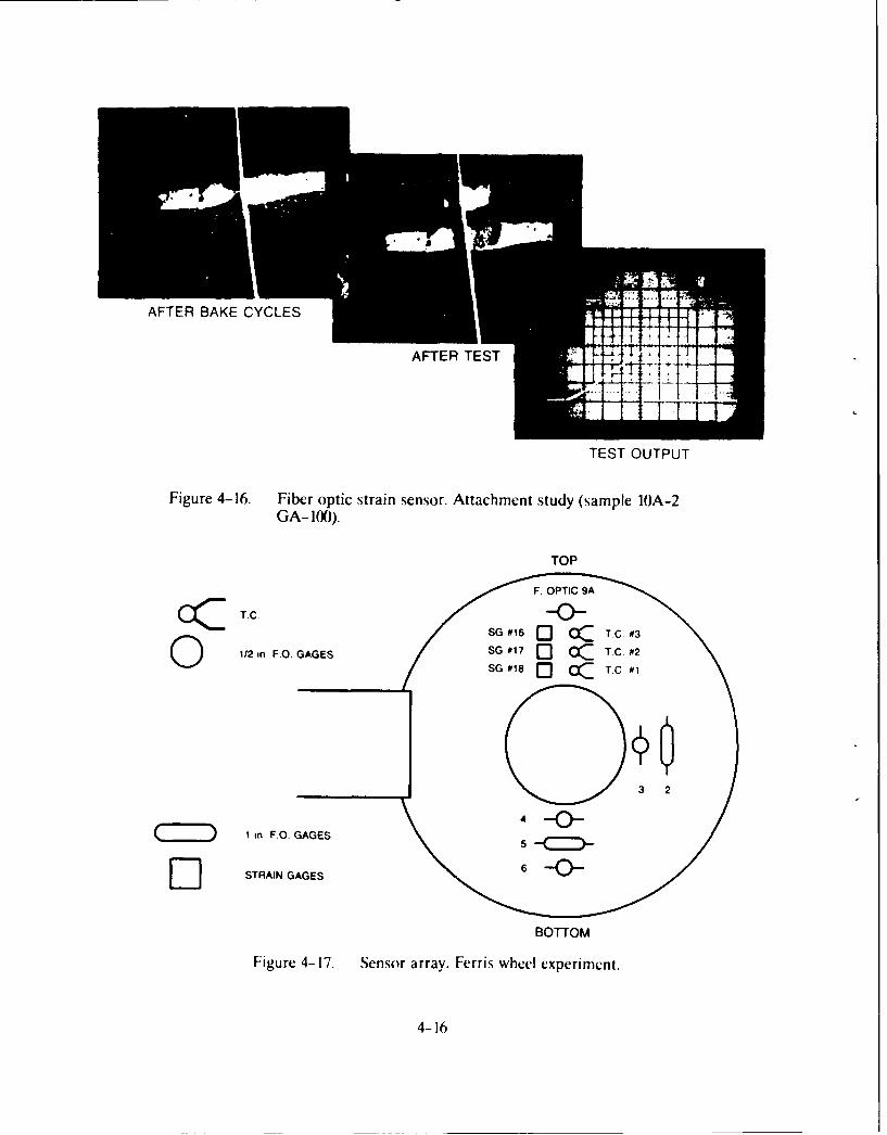
AFTER BAKE CYCLES 1 -+

TEST OUTPUT

Figure 4-16. Fiber optic strain sensor. Attachment study (sample 10A-2GA- 100).

TOP

C T.C,

O1/2 in F.O. GAGESSG#70 C . 2

0

I in. F.O. GAGES5

Fr1 STRAIN GAGES

BOTTOM

Figure 4-17. Sensor array. Ferris wheel experiment.

4-16

TABLE 3. SENSOR INVENTORY; FERRIS WHEEL EXPERIMENT

* 6 PdCr static thin film strain gages

* 6 FeCrAl static thin film strain gages

* 6 Ni/30Cr dynamic thin film strain gages

* 6 twin-core fiber optic strain and temperature sensors

* 6 standard electrical strain gages

6 type K thermocouples

Wavelength multiplexing was selected to implement two color transmitter operation; a helium

neon laser (633 nm) and a laser diode (830 nm) were coaxially combined with a dichroic beam

combiner. After equal division with a non-wavelength-sensitive splitter, two sets of beam-to-fiber

matching optics enabled us to excite two sensors simultaneously. The receiver system utilized a

dichroic splitter to separate the signals from each output lead. Therefore, to complete the

measurements we recorded 8 detector signals (2 sensors, 4 output leads, 2 colors) in addition to the

signals from the supporting instrumentation on a computer-supported acquisition system backed up

by an FM instrumentation tape recorder (Table 4). All signal processing was conducted after the tests.

The instrumentation is shown in Figure 4-18.

TABLE 4. INSTRUMENTATION; FERRIS WHEEL EXPERIMENT

HP-85 with dual floppy disk storage

* HP-3497 data acquisition unit

* 44427A(3) plug-in for strain gage bridge completion/measurement

44422A(1) plug-in for thermocouple and twin-core sensor measurement

* multi-channel FM tape recorder for bzzkup

4-17

-e'8 4@

.Q,

EXCITATION OPTICS

RECEIVER OPTICS

Figure 4-18. Tin-core optical fiber sensor. Ferris wheel Experimental Facility.

Figure 4-18 also shows a disk positioned within the Ferris wheel test facility (at Pratt & Whitney,

West Palm Beach, Florida). Hydraulically driven rods are used to simulate spin loads applied to the

disk. Table 5 correlates rod loading levels with strain applied to the sensor locations. A movable pipe

structure is used to support a clamshell oven in position, covering each side of the disk. The entire disk

and support system is rotated in an oscillatory fashion at 1 r/min to maintain uniform elevated

temperatures on the disk.

4-18

TABLE 5. LOAD AND STRAIN RELATION

Ferris wheel Experiments

Load (N) Strain (4E)

2,896 459( 2)

5,792 923( 31~)8,688

1,391( -_4-1/}

I 5/ + 4711.584 1, 853(- 53

1A)2,321(_ + 9

The test program conducted with this facility is shown in Figure 4-19. Highlights of the most

important results of the Ferris wheel experiment are reviewed in this section. An outline narrative of

all test results is contained in Appendix A: Ferris wheel Data Base.

Characteristic sensor response (unprocessed data) to 589 K is illustrated in Figure 4-20 which

presents the core contrast function plotted against the approximate temperature of the disk. Clearly

present is the cosine discriminant of the twin-core sensor response with a contrast limitation for this

device equivalent to about 0.5. The signal can be linearized simply by application of an arccosine

inversion. While at 589 K, a load survey was conducted. Figure 4-21 shows excellent sensor load

response.

In subsequent tests, sensor operation was verified above 922 K while slippage of the attachment

was observed during the load survey. For example, Figure 4-22 provides one sensor signal which

responds nicely with the increase in temperature from ambient conditions to more than 922 K.

However, on the way down in temperature after a load survey, there is an offset in the quiescent signal.

We believe that this occurred as the result of the sensor slipping within the ceramic cement during the

load survey. That survey is plotted in Figure 4-23, where we notice no effective sensor response to

strain even though it is obviously working as evidenced by the thermal response.

4-19

14KLOAD (LBF)

12K - -- TEMP (K) F 922

10K- A8118K I I 18K I 700I I I 11 a, I

< 6K I I | i I 589 wu

4K 472 I S 1 3l

2K 5/ 6 - S516 S1/3 S5/6 S516 S5/6y 6 1 S6 36

0 W 01 2 3 4 5 6 7 8 9 10

RUN NO.

Figure 4-19. Ferris wheel test program.

0.6

0.5 M po U I

ooCI,<~ 0.4I-

o 0.3 -

00.2

0.1 I I I I I0 422 585

TEMPERATURE, deg K

Figure 4-20. Twin-core optical fiber sensor. Temperature response. Ferriswheel data, run No. 4. sensor 6, 633 nm.

4-20

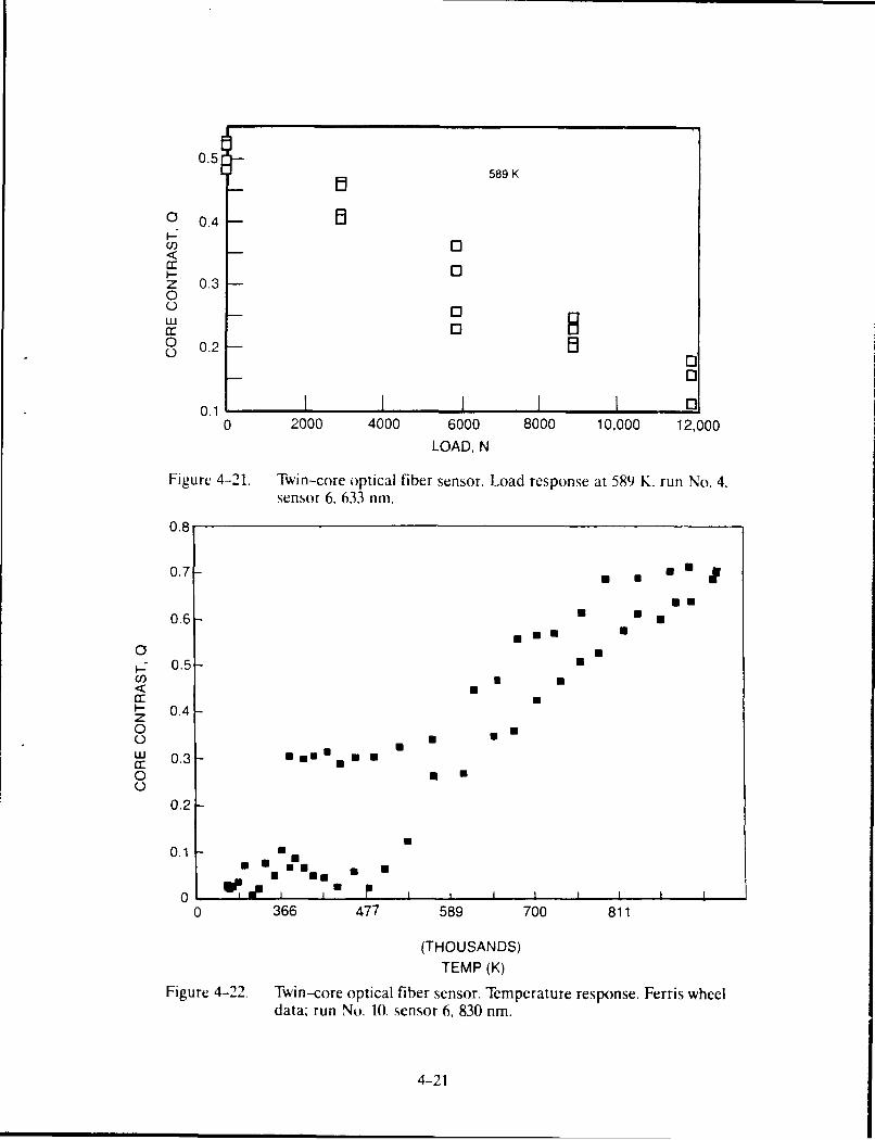
0.5

1 589 K

o 0.4 -

U)0

0z 0.30C-)o WB0 0.2

0

0.1 I I I I0 2000 4000 6000 8000 10,000 12,000

LOAD, N

Figure 4-21. Twin-core optical fiber sensor. Load response at 589 K, run No. 4,sensor 6, 633 nm.

0.8

0.7 -usE1

im

0.6 - mE

O Ui_: 0.5 M

,<

- 0.4-z0C)u 0.3- sonn *O mm•C-)

0.2-

0.1 .

00 366 477 589 700 811

(THOUSANDS)

TEMP (K)

Figure 4-22. Twin-core optical fiber sensor. Temperature response. Ferris wheeldata; run No. 10. sensor 6, 830 nm.

4-21

In summary, the twin-core optical fiber sensor survived the simulated engine test conditions as

demonstrated by the signals and the before/after photographs in Figure 4-24, verifying our selection of

sensor materials and coating materials. Unfortunately, problems were encountered with the

attachment of the devices to the disk and with reliability of some of the instrumentation. Most of the

significant issues were further addressed during the spin rig experiments.

5. ROTATING TESTS--THE SPIN RIG EXPERIMENT

In support of instrumentation developments discussed in this section, the twin-core sensor was

fabricated with different dimensions for the Spin rig experiment. Operational wavelengths for this test

phase were changed such that both were in the near infrared region. As a result, the waveguide

dimensions could be increased, yielding larger throughput signals. Table 6 lists the parameters for the

new sensor measured by two methods, with an optical microscope and with an index profiler. When

the preform for the sensor is assembled with an outside diameter of the order of 2 cm, the spatial

0.68

1220oF

0.67

0 0.66-I-Cj)

z 0.65--0 U

o 0.74

0.63--

0.62 I1 I060 2 4 6 8 10(THOUSANDS)

(LOAD (LBF)

Figure 4-23. Twin-core optical fiber sensor. Load response at 933 K. Ferriswheel data: run No. 10, sensor 6, 830 nm.

4-22

4-2

distribution of the index of refraction across the diameter of the sensor is representative of a perfect

step function for each core. However, the extrusion process used to fabricate the functional devices

with final outside dimensions of the order of 186um can cause some diffusion of the germanium

dopant from each core into the surrounding cladding. The resulting spatial distribution of the index of

refraction is no longer a perfect step function but representative of a distribution between step and

Gaussian. This fact has an affect on the actual sensitivity of the device in comparison with the

predicted response. Initially, a detailed analytic model was used to predict the response of the sensor.

The analytic model assumes either a step index distribution or a Gaussian distribution. The predicted

sensitivities of the sensor to temperature and strain changes are given in Table 7. This table also lists

the anticipated total signals for a device subjected to a thermally induced strain which results from

attachment to IN-100 elevated to 866 K and to a mechanically induced strain of 2000 microstrains.

Note that the core contrast (Q) phase shift, A4, is calculated as twice the beat phase shift, 60 . We

observe that there is a significant difference in the response of a device with a step function

distribution compared with a Gaussian distribution and this difference depends on wavelength.

TABLE 6. SPIN RIG SENSOR PARAMETERS

Optical Microscope Measurements

OD = 186 gtm

d = 6.51 4m

a - 1.77 4m

Index Profiler Measurements

OD = 185.5 gim

d = 6.1 gm

a = 1.55 gm

NA = 1.43 gim

4-24

TABLE 7. ANALYTICALLY PREDICTED, UNATTACHED CALIBRATION

CONSTANTS AND RESPONSE(PER INCH OF SENSOR LENGTH)

750 nrn; step 750 nm; gauss 830 nm; step 830 nm; gauss

(%/u() 1.5 x 1()-3 2.5 x 1- 3 2.0 x 10-3 3.0 x 1Q- 3

df

d o ) -. 1. x 10-2 -4.5 x 10-2 -1.8 x 10- 2 -4.5 x 10-2dlV

SO(20XX) u moch) .0i 10 8.0 12

u( thermo)t 24 40 32 48

(IN- l(E% 86K)

'(()(K temp) -19 -54 -22 -54

lOWt '0 11 -4 18 6.0

Since the index distribution is neither perfectly step nor perfectly Gaussian, a new detailed

empirical modelling method was implemented to develop predictions for the effective calibration

constants. The modelling process is outlined in Figure 4-25. To begin with, the response to a

temper':ture perturbation is shown to be a function of the derivative of the coupling factor F with V On

the other hand, the strain coefficient is a function of F and dF/dV. These functional relationships

provide the clue to a valuable method of using nondestructive test data from a real sensor with a real

index distribution for derivation of the calibration constants. If Q is measured as a function of

wavelength, A. we should have data that takes into account core-to-core coupling for the effective

index distribution and then be able to derive the effective calibration constants. This is feasible

because of the simple functional relationships shown in Figure 4-25.

The wavelength response for a specific sensor is shown in Figure 4-26. Next, Figure 4-27 shows

do/dA for this data and for a second, longer range data set. Then dF/dV and F(V) can be derived

(Fig. 4-28). These finally yield do/dc and do/dT of Figure 4-29, the calibration coefficients. What we

discover is that the effective calibration coefficients fall between those of the analytically predicted

4-25

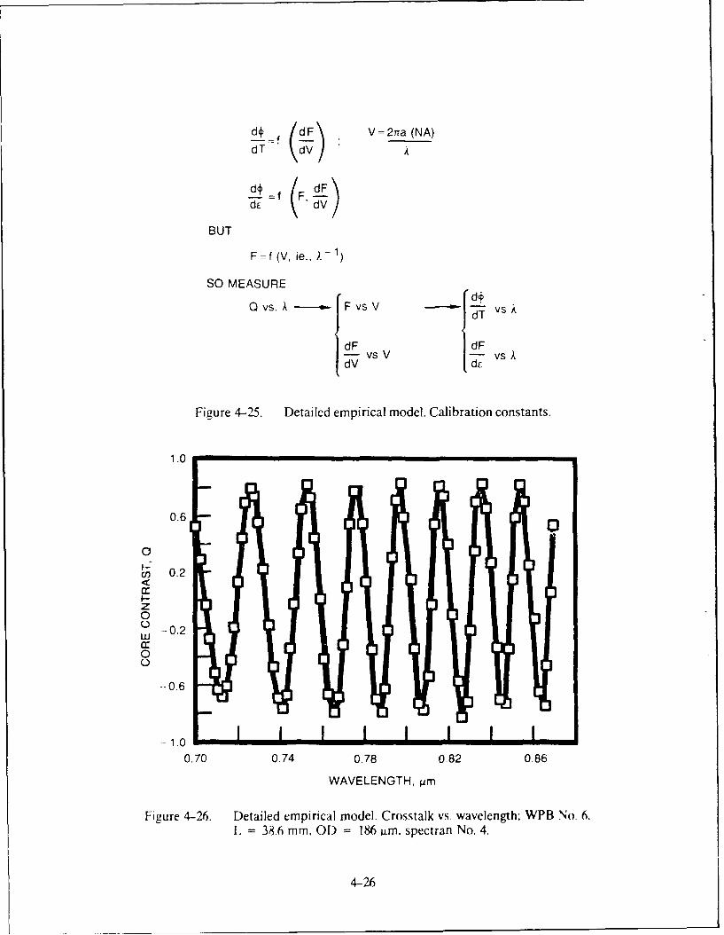
/dF\ V = 2Tna (NA)d T dVA

±d=f F, dF\

BUT

F =f (V, ie., A)

SO MEASURE

Qvs dTvs

-Fvs V vs AIdV I

Figure 4-25. Detailed empirical model. Calibration constants.

1.0

0.6

U)0.2

I--z0

0.2

0

-0.6

--1.00.70 0.74 0.78 0.82 0.86

WAVELENGTH, ;im

Figure 4-26. Detailed empirical model. Crosstalk vs. wavelength; WPB No. 6,L = 38.6 mm, OD =186 a~m, spectran No. 4.

4-26

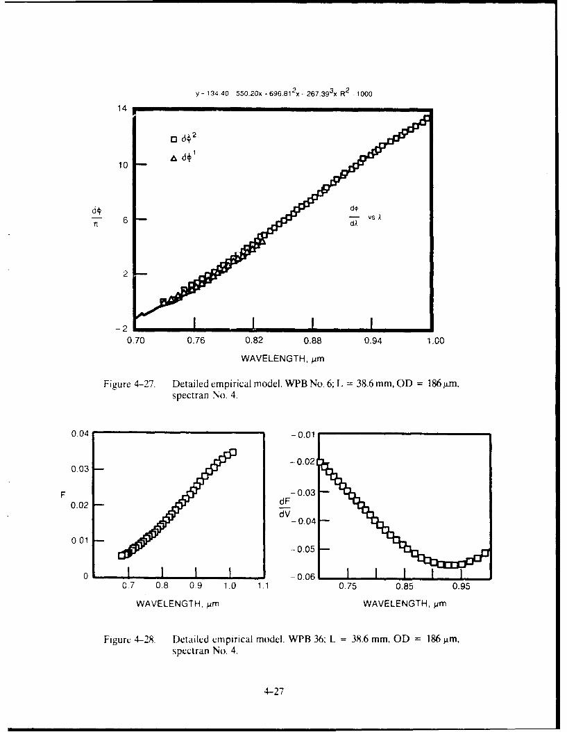
y= 134.40 550.20x-696.812x-267.393 x R2

- 1000

14

o d2

10

7 6 dA

2

-20.70 0.76 0.82 0.88 0.94 1.00

WAVELENGTH,/pm

Figure 4-27. Detailed empirical model. WPB No. 6; L = 38.6 mm, OD = 186 pm,spectran No. 4.

0.04 -0.01

-0.020.03 -

F - 0.030.02 - dF

dV_ 0.04

0.01-0.05 -

0I ! I I -o_ _ __o6_

0.7 0.8 0 9 1.0 1.1 0.75 0.85 0.95

WAVELENGTH. pim WAVELENGTH, ym

Figure 4-28. Detailed empirical model. WPB 36: L = 38.6 mm, OD = 186 gim,spectran No. 4.

4-27

0.001 -0.01

0.003 -0.02

d+~ 1 d4 (1

_d dTfl

0.002 -0.03

o o -0.04 I I I I I0.75 0.85 0.95 1.05 0.75 0.85 0.95 1.05

WAVELENGTH, ym WAVELENGTH, pm

Figure 4-29. Detailed empirical model. Strain and temperature sensitivitycoefficients. WPB No. 6: L = 38.6 mm, OD = 186 Atm, spectran No. 4.

values for step and Gaussian index distributions; more step like at shorter wavelengths where the

optical field is more tightly contained within the core and more Gaussian-like at longer wavelengths

where the optical field tends to spread out into the cladding. Data verifying the temperature response

is given in Figure 4-30.

To implement the rotating test phase of these new sensors, two additional key areas required

attention: attachment and miniaturization of the supporting electronics. To begin with, the Ferris

wheel phase of testing proved that the twin-core optical fiber sensor survived operation above 922 K,

but indicated slippage in the attachment of the device to the disk above755 K. Resolution of this design

issue is portrayed in Figure 4-31. Ceramic cement attachment has been superceded by a method

called flame spraying. During the flame spray attachment process (performed by Pratt & Whitney.

West Palm Beach, Florida), the sensor is held in contact with the prepared surface of the disk while

molten droplets of aluminum oxide are blown over the sensor gage length and the adjacent portion of

the (li4k. As the ceramic droplets impact the working surfaces, they bond together, freeze, and build

up to a durable coating. Attachments assembled in this form have proven integrity which exceeds

ceramic cements under harsh conditions.

4-28

3.06 x 1

66

2.17

I>JTERPRETED SENSOR

TEMPERATURE (0 C) 9

x01.29 002kx

x2

x o

0.40 X1 R.I.1.. 0 ...0.

0.40 0.73 1.05 1.38 1.70 2.03 2.35 2.67 3.00 x 1 o2

MEASURED THERMOCOUPLE TEMPERATURE ('C)

Figure 4-30. Twin-core optical fiber sensor. Temrtrature response; WPB No. 6,unattached.

Figure 4-31. TWin-core optical fiber sensor. Flame-spray attachment toModified F1OO turbine disk.

4-29

A significant change was also required in the supporting instrumentation. For instance, the large

rack of equipment shown in Figure 4-18 cannot be accommodated in the spin rig. During planning of

the rotating tests, an appropriate optical slip ring for use with single mode sensors was not available;

hence, the system was designed around use of an electrical slip ring to transfer power and signals

to/from the rotating disk. This approach necessitated placement of the laser sources in the hub of the

test piece. The required miniaturization was accomplished by using two laser diodes arranged to fit on

a small transmitter circuit board. Again, wavelength multiplexing was implemented. The first version

of the transmitter used microlenses and a coupling prism, shown in Figure 4-32 prior to encapsulation.

This unit was destroyed in an early run of the spin rig after the mechanical support for the

instrumentation can failed, precipitating a catastrophic imbalance in the spinning system. The rebuilt

transmitter is shown with a different geometry in Figure 4-33 where a narrow-band optical fiber

multiplexing coupler was used for beam combining. The temperature of the diodes was actively

regulated with a thermoelectric cooler. The transmitter board mates with two receiver boards, each

containing microlens/microprism wavelength demultiplexers and other circuitry (Fig. 4-34). The

boards mount in the hub of the disk and receive power and control signals on wires installed in the

drive shaft. All circuitry was encapsulated in high temperature epoxy for stable operation during

rotationally-induced g-fields to 1000 g. These advances in instrumentation development are shown in

the composite photograph of Figure 4-35, along with photographs of the installed disk and the spin rig

facility. The spin rig (Section VI) facility consists of a large vacuum chamber with a~drive system to

spin the disk, an induction heater to elevate the disk temperature and a slip ring to communicate with

instrumentation in the spinning work frame. The spin rig test program is summarized in Figure 4-36

which indicates a limitation in conditions, short of the 922 K and 13,200 r/min goals. A vibration,

which could not be conveniently damped, limited the spin rate to less than 8000 r/min. After balancing

attempts, several breaks were discovered in interconnecting fiber between the three circuits boards.

This limited the experimental conditions to runs up to 589 K. At the time of the interconnecting fiber

failure, the sensors and the encapsulated transmitter and receiver systems were functional. Funding

limitations have obviated repair and further experimentation.

4-30

Figure 4-32. TWin-core optical fiber sensor. Miniature 2 - x transmitter;version 1.

Figure 4-33. Twin-core optical fiber sensor. Miniature 2 - k transmitter;version 2.

4-31

Figure 4-34. Twin-core optical fiber sensor. Miniature 2 - x receiver.

2 OPI-lTANSMI ER

-- -- -/,AND RUE LII W L

Figure 4-35. Twin-core optical fiber sensor. Spin rig experiment.

4-32

10K 811- ROTATION RATE (RPM)

8K - - TEMP (K) - 700

6K B -589

ROTATION 6 TEMP, K

RATE, RPM4K - 477

2K - 366

01 2 3 4 5A 5B 6

RUN NO.

Figure 4-36. Spin rig test program. Build 3/4 B.

Representative data samples from the spin rig experiment begin with Figure 4-37. This example

provides raw sensor data from the system spinning at 1000 r/min while the temperature was increased

from ambient conditions to more than 589 K and then cooled. Next. the temperature was held

relatively stable at 422 K. At this temperature, Figure 4-38 shows the sensor response to acceleration

in spin rate from 10X) r/min to nearly 7(XJ r/min. A similar test sequence is provided in Figure 4-39 for

operation at 589 K. In all three cases, the sensor response shows what appears to be hysteresis.

However. other sensor measurements at the time of this experiment indicate that the response is not

sensor hysteresis, but is indeed related to the str' s state of the disk. The disk is not heated uniformly

from the blades to the hub, and therefore a radially distributed strain gradient exists. The temperature

distribution :hat induces this gradient is time dependent. Therefore the radial strain distribution on

the disk web is different during the acceleration run in comparison with the deceleration sequence.

The twin-core sensor was capable of detecting the effect of this evolving stress state.

6. DISCUSSION

The purpose of this section is to discuss the results from the spin rig experiment, comparing the

twin-core sensor with other sensors which were available during appropriate ranges of conditions. The

4-33

1.0BUILD 314 B

0.8 1000 rpm i

0.6

CORE 0.4

CONTRAST,

0.2 U

0

-0.2 I. I I i Io 366 477 589

TEMPERATURE, deg K

Figure 4-37. Twin-core optical fiber sensor. Temperature response at 1000r/min. Spin rig data; run No. 5, 830 nm.

0.6 LBUILD 3/4 B

422 K

0.4

0.2

CORECONTRAST, 0

Q -0.2 i

-0.4

-0.6

-0.8

1K 3K 5K 7K

ROTATION RATE, rpm

Figure 4-38. TWin-core optical fiber sensor. Load response at 422 K. Spin rig

data; run No. 5, 830 nm.

4-34

I BUILD 3/4 B

0.90 589 K

0.80 - !CORE 0

CONTRAST,Q

0.70 - I

0.60 - I I I I I0 2K 4K 6K

ROTATION RATE, rpm

Figure 4-39. Twin-core optical fiber sensor. Load response at 589 K. Spin rigdata, run No. 830 nm.

Ferris wheel experiment is not included in the analyses presented here, owing to the fact that it was a

risk reduction implementation emphasizing a shake out of installation and instrumentation issues. On

the other hand. the spin rig tests provided a more carefully controlled data base for correlation of

different sensors.

Figure 4-40 compares the output of various strain sensors attached to the disk at a radius of 152

mm as a function of variations in nominal web temperature. The parameter used for comparison is the

difference in strain reading between the high speed 6600 r/min case and the reference low speed

I(X0-12X) r/min case. The strain difference parameter is plotted as a function of temperature to

minimize drift and zero shifts from various sensors. The shaded region on the graph indicates the

theoretically predicted strain differences for a possible range of anticipated thermal gradients on the

disk. It is necessary to present the predicted results as a range of values because insufficient data were

available to document the exact state of thermal gradients which can be expected to impact the local

strain measurements from each sensor. The thermal gradients result from nonuniform heating of the

4-35

KEY

SYMBOL BUILD NO SENSOR TYPE

O 2 CHINESE ALLOY WIRE GAGE

O 2 THIN FILM GAGES nEPOSITEO ON FOL BACKING

3 THIN FILM GAGESODEPOSITEG ON FOIL BACKING

1' 2 STRAIN BY SPECKLE PHOTOGRAMMETRY

0 1 COMMERCIAL STRA.N GAGED I TWIN CORE OPTICAL FIBER SENSOR

CIRCUMFERENTIAL STRAIN

2 0 0 - O FE N . ,C N,. S C -.,. E C EL

EU

0

1000

0 .. .....I-

z

4F-

0Z

-1000 1200 300 400 500 60C

TEMPERATURE (K)

Figure 4--40. Sensor comparison 152 mm radius, 6600 r/min.

disk by the induction heating element during the time of the tests. Furthermore, we must remember

that the thermal gradients during acceleration portions of a test (early in the experiment) will be

different from deceleration portions of a test (late in the experiment) because of time development of

.he grawients.

To accomplish the calibration of the twin-core optical fiber sensor, the measured Q response

parameter was converted to a normalized Obar response parameter to accommodate nonidea)

characteristics of the devices. The Obar response follows a cosine discriminant. Hence, the arccosine

function i i used next to create a phase parameter which can be calibrated and is linear in strain or

temperature.

During the spin rig experiments, one of the laser diodes in the twin-core sensor instrumentation

package did not operate properly, hampering attempts to apply the unique calibration methods of

Section 5 to this data. As an alternative, the twin-core sensor data was referenced to the room

temperature data of the speckle photogrammetry system and then plotted to yield Figure 4-40. The

4-36

two types of data show similar trends except for the room temperature deceleration twin-core sensor

measurement. This measurement is somewhat erratic because it comes from the first test and exercise

of the attached sensor; a situation which typically yields some additional hysteresis-like effects.

Other comparisons between the ti'in -core sensor data and speckle phot"gramlro;y data were

conducted. For instance, the strain response at 422 K as a function of disk rotation rate is shown in

figure 4-41. Note that the x-axis is plotted as the rotation rate squared divided by 1,(00,000. Strain on

the disk should be linearly proportional to this parameter. Indeed this appears to be verified with the

acceleration data. In cone.rast. the deceleration data show a hysteresis-like effect which resuts from

the time-dependent thermal stresses imposed on the spinning disk by the nonuniform heater. A least

squares algorithm was used to calibrate the twin-core response to the speckle data.

Similar results are shown in Figure 4-42 for a comparison at 589 K. The key difference here is that

the speckle experiment encompassed a much harsher, more extensive range of conditions, causing

more hysteresis in the data. Since the twin-core sensor encountered more limited conditions, the

hysteresis eflects are less severe.

4-37

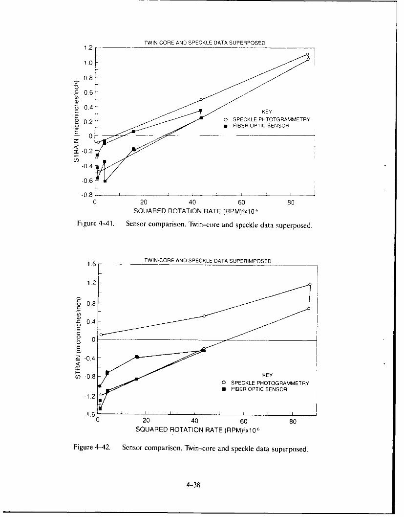
TWIN-CORE AND SPECKLE DATA SUPERPOSED1.2 - _ _ _ _ _ _ _ _ _ _ _ _ _ _ _ _ _ _ _ _ _ _ _ _ _ _

1.0

0.8

0.6-

*~0.6

P 0.2

E 0z

-0.2U)~

-0.4

-0.6v

-0.8

0 20 40 60 80SQUARED ROTATION RATE (RPM) 2xl 06

Figurc 4-41. Sensor comparison. Twin-core and speckle data superposed.

1.6 TWIN-CORE AND SPECKLE DATA SUPERIMPOSED

1.2

o0.8

~0.4

z -0.4

KEYcn 0.8-O SPECKLE PHOTOGRAMMETRY

0 FIBER OPTIC SENSOR

-1.2

-1.6-0 20 40 60 80

SQUARED ROTATION RATE (RPM) 2X 0 6

Figure 4-42. Sensor comparison. Twrin-core anid speckle data superposed.

4-38

APPENDIX AFERRIS WHEEL DATA BASE

4A-1

APPENDIX AFERRIS WHEEL DATA BASE

Figures 4A-1 through 4A-4 represent the primary results from the twin-core optical fiber sensor

during the Ferris wheel experiments. Each figure indicates the sensor response at two wavelengths (633

nm and 830 nm) for various sensors (S5 and S6)as they react to a temperature increase in the disk, and

then the strain response as the heated disk is loaded. All responses are given in terms of the crosstalk

parameter Q. Further, each figure provides an expanded view of the most important data from the test.

4A-2

(a) TEMPERATURE RESPONSE (b) STRAIN RESPONSE AT 463 KFERRIS WHEEL DATA FERRIS WHEEL DATA

RUN NO. 3 RUN NO 3160 S6 (633)

0.8 S6(333)0 S5 (830) S5 (830)

0.6 S6 (830) S6 (830)

0.4 - 5 (633) S5 (633)

0 .2,-0.2 -- -. -

-C i 0_6_,H,_--.,,____________________,__,_-- .8

-.-. __ _

-1.0 I I300 350 400 450 500 550 0 b 10 15 20 25 30 35 40

TEMP (K) LOAD (THOUSANDS)(N)

(c) TEMPERATURE RESPONSE (d) STRAIN RESPONSE AT 463 K

FERRIS WHEEL DATA FERRIS WHEEL DATA

RUN NO. 3- SENSOR 6 RUN NO. 3- SENSOR 6

633 nm 633 nm

0.50-

0.4P

0 .3 1k 0 .4 0

0 I0____________________ 1 0.20 I I I I I i

300 350 400 450 500 0 5 10 15 20 25 30 35

TEMP (K) LOAD (THOUSANDS)(N)

Figure 4A-1. Twin-core optical fiber sensor.

4A-3

(a) TEMPERATURE RESPONSE (b) STRAIN RESPONSE AT 605 KFERRIS WHEEL DATA FERRIS WHEEL DATA

RUN NO. 4 RUN NO 4

1. ,S6 (633) S6 (830) S6 1633)0. S5 (830) S5 (633) S6 (830)

0 61 S5 (830)

0. 4 1,

-0.8'

30 400 500 600 700 0 5 10 15 20 25 30 35 40

TEMP (K) LOAD (THOUSANDS)

(c) TEMPERATURE RESPONSE (d) STRAIN RESPONSE AT 605 KFERRIS WHEEL DATA FERRIS WHEEL DATA

RUN NO. 4 -SENSOR 6 RUN NO. 4 -SENSOR 6633 nm 633 nm

0.60i

0.50-050

flu 0.40-i

0.40- * U00

0.30-0.0

0.20 *0.20-

0.101 1V 0.10I________________ _____

300 400 500 600 0 5 10 15 20 25 30 35TEMP (K) LOAD (THOUSANDS)

(N)

Figure 4A-2. 'P~vin-core optical fiber sensor.

4A-4

(a) TEMPERATURE PROFILE (b) STRAIN RESPONSE AT 910°FFERRIS WHEEL DATA FERRIS WHEEL DATA

RUN NO 6 RUN NO. 61 .0 - S 6

0.8-. S5 (830) S6 (633)

0.6 15(633) S5 (830)

0.4 S6 (830)

0.22 S5(633)

o 0~ ; - "-__ __~__ _ __ _

-0.4-- 0.61_"--_______-_____.. ...

300 400 500 600 700 800 0 5 10 15 20 25 30 35 40 45LOAD (THOUSANDS)

TEMP (K) (N)

(c) TEMPERATURE RESPONSE (d) STRAIN RESPONSE AT 910-FFERRIS WHEEL DATA

FERRIS WHEEL DATA RUN' NO. 6 - SENSOR 5RUN NO. 6 830 nm

1.0 -0.660.8 S6 (633)

0.6 S6 (830) -0.67-

0.4- -0.68!0.2 1O.'____ - - -0.69- ,•

-0.2- /

-0.4 ..----- -- -0.70-

-0.8 I - 0 .721 I I I I I I

300 400 500 600 700 800 0 5 10 15 20 25 30 35 40 45

TEMP (K) LOAD (THOUSANDS)(N)

(e) TEMPERATIRE RESPONSE (f) STRAIN RESPONSE AT 910°FFERRIS WHEEL DATA FERRIS WHEEL DATA

RUN NO 6- SENSOR 5 RUN NO. 6- SENSOR 6

830 nm 0.3 633 nm

-0.11 0.2-0.-2 •*

-...~ . . .- 0.2_ , 0.1

-0.3,Q -0-4-"

- 00.51

_ " " -0.2 -

- 7j- * -0.3[

-0.81 I I I -0.41 ' I , I300 400 500 600 700 800 0 5 10 15 20 25 30 35 40 45

TEMP (K) LOAD (THOUSANDS)(N)

Figure 4A-3. Twin-core optical fiber sensor.

4A-5

(a) TEMPERATURE RESPONSE (b) STRAIN RESPONSE AT 933 KFERRIS WHEEL DATA FERRIS WHEEL DATA

RUN NO. 10 RUN NO 101.0 _0.8

0.60.4

0.2 5Q 0 ------------------

- 0.2-

-0.4 S6 (830) S6 (830)

- 0.6 S6 (633) S6 (633)-1.0- 0 .8I I I I I I I I

200 300 400 500 600 700 800 900 1000 0 5 10 15 20 25 30 35 40 45

TEMP (K) LOAD (THOUSANDS)(N)

(c) TEMPERATURE RESPONSE (d) STRAIN RESPONSE AT 933 K

FERRIS WHEEL DATA FERRIS WHEEL DATA

RUN NO. 10 - SENSOR 6 RUN NO. 10 - SENSOR 6

830 nm 830 nm

0.8 0.68

0.67-0

0.6-• • 0.66-

0 0.65-

0.64,-0.2- 0 0.63,- a

0 *""° • l I I I I 0 .6 2 I I 1i I I I00.200 300 400 500 600 700 800 900 1000 0 5 10 15 20 25 30 35 40 45

LOAD (THOUSANDS)

TEMP (K) (N)

Figure 4A-4. Twin-core optical fiber sensor.

4A-6

N' RESISTANCE STRAIN GAGES

1. INTRODUCTION

Two types of small (1/8 in) high-temperature resistive static-strain gage were installed on turbine

disks designed for aircraft engines and were hot spin-pit tested to 950 K and 2(XX) microstrain at 30,000

G centripetal acceleration. These were the first reported trials of these new gages on rotating parts.

One type is a FeCrAI alloy gage in wire form, developed in China. The other is a PdCr alloy gage. in

sputtered-film form, currently being developed at United Technologies Research Center under NASA

contract.

Both types were mechanically durable. The results showed some improvements over previous

attempts to obtain rotating static strain measurement at high temperature with small resistive gages.

The long-term goal of uncertainty below 2M%) microstrain at temperatures above 660 K has not yet been

approached. The performance limiting factor for the FeCrAI gages is believed to be metallurgical

phase-stability and for the PdCr gages insufficient oxidation protection.

Further development of the PdCr alloy gage system is recommended because the gage alloy itself

is metallurgically stable. The development required includes improved oxidation protection and some

moderate temperature compensation.

2. OBJECTIVE

A major long-term objective in the development of aircraft gas turbine engine components -ind

hypersonic aircraft structures is the measurement of static strain under transient nonisothermal test

conditions at temperatures above the present 660 K limit of available resistive static strain gages.

Strain uncertainty of 200) microstrain or less is required in at least a 2000-microstrain measurement

range. In aircraft engines, the measurements are required on both stationary and rotating components

(vanes, blades, turbine disks). A recent review of these requirements was presented by Stange (Ref, 1).

Typical test exposure includes many transient loading sequences, from a few seconds to a few min

in duration, during which temperature is simultaneously varying from near cryogenic (in the case of

hypersonic aircraf.) . a high as + 1300 K. The peak strains occur in small localized areas near holes,

fillets, airfoil roots, and thinwall sections. Spatial resolution of 3 mm or less is required.

5-1

The technique for static strain measurement used most widely and successfully at lower

temperatures is the resistive strain gage. At present, no small strain gage is available with capability

even approaching the desired high-temperature static strain capability above 660 K, the temperature

of onset of metallurgical phase changes in commonly used strain gage alloys.

Development of improved small resistive static strain gages for use above 660 K has continued. In

the present program the state of development of two types was dc-nonstrated.

3. STATE OF THE RESISTANCE STRAIN GAGE ART

The typical resistance strain gage sensor (Fig. 5-1) is a grid of fine wires, sputtered films, or foils.

bonded to the component under test, with suitable lead wires extending to an electrical Wheatstone

Bridge resistance-measuring circuit. A three-wire connection is used to cancel the effects of lead wire

resistance changes.

The measure of strain is the fractional change in strain gage resistance, AR/R, due to mechanical

strain, A L/L. The resistance strain gage method therefore depends on accurate knowledge of the gage

factor AR/R / AL/L, and on insensitivity of the electrical resistance, R, to other influences such as

temperature and erosion. The gage factor for metals is about 2 and the range of strain measurement of

interest is usually about 2000 microstrain. Therefore the range of resistance changes is typically 40M)

microhms/ohm.

The strain gage alloy must be chemically stable and oxidation resistant, relatively low in

temperature coefficient of resistance (ter), and metallurgically stable.

At temperatures up to about 660 K. low-tcr strain gage alloys such as Ni2OCr, Evanohm, FeCrAI

and Cupron provide the desired stability and accuracy. Figure 5-2 shows examples of short-term

reversible metallurgical drift characteristics of high-temperature strain gage alloys. Note that in the

range 660 K to 920 K the drifts are as large 10,000 microhms/ohm. The figure shows the drift in 16 hours

at each test temperature, after fast cooling from 920 K to test temperature. Not shown is the change in

resistance from 920 K to the test temperature before the start of the drift test and the change in

resistance from test temperature to 920 K at the end of each drift test. At 920 K the gage resistance

5-2

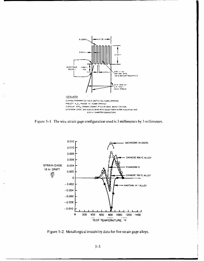
6 LOOPS ~-0 130 ~

RESISTAN4CE 0 050 I

WELDE D 44I...SHP-700C WIRE120 9 SENSOR RESISTANCE

F Al RIBBON

INSTALLATION

SURFACE PREPARATION N,CA, IMETCO '43) FLAME SPRAYED

PRECOAT A'20 3

IROKIDE HI) FLAME SPRAYED

OVERCOAT AIPO14 CERAMIC CEMENT (PI2.2 ON BARS BEAN H ON DISK)

EXTENSION LEADS 3CN. CLAD Cu, WIRE WITH OALSS FIBER OUTER INSULATION A.ND

0 012,I DIAMETER CONDUCTORS

Figure 5-1. The wire strain gage configuration used is 3 millimeters by 3 millimeters.

0.012 -. NICHROME (N1200R)

0.010 I'

0.008

0.00 - 4-M*-CHINESE 800-C ALLOY

STRAIN-GAGE 0.004- VNHS1hrDIT 0.002 -'ll 'lp itCHINESE 700 C ALLOYR 0 % I

-0.002 - KANTHAL A-1 ALLOY

-0.004

-0.006

-0.'008

-00101

G 200 400 600 800 1000 1200 1400

TEST TEMPERATURE, OF

Figure 5-2. Metallurgical instability data for five strain gage alloys.

5-3

recovers to its previous 920 K value within a few minutes, for these alloys. About 10% of th total

16-hour drift ,ecurs in the first few minutes at each test temperature. The dat? are from tests at Pratt

& Whitney over the past few years.

The selection of gage alloys has narrowed historically to concentrated alloys (for low tcr).

preferably with featureless phase diagrams at all temperatures and therefore free from formation of

chemical compounds, reordering of the lattice structure, or magnetic transformations, to avoid the

drifts shown in Figure 5-2.

The state of the art has centered recently on two alloy families. One is the historically promising

FeCrAI family (iron-chromium-aluminum) with added modifications and the other is the recently

investigated PdCr (palladium-chromium) family. FeCrAI offers low tcr of about 15 x 1() - 6 K-1 and

excellent oxidation self-protection but marginal metallurgical stability. An example is given in

Figure 5-3. where resistance change versus temperature of a FeCrAI alloy (examined by UTRC

(Ref. 2)) is sensitive to heat treatment time at elevated temperature. The PdCr alloys offer great

stability at high temperatures but marginal tcr of about 180x 10- 6 K- 1 and less oxidation resistance. An

example of excellent metallurgical stability is given in Figure 5-4, where a PdCr alloy (from the same

UTRC program (Ref. 2)) was insensitive to heat treatment time at high temperature or to rate of

coling or heating.

4. APPROACH TO DEMONSTRATION TEST

In this program, a series of several high-temperature spin tests of instrumented turbine disks,

from a 20.000-pound-thrust military gas turbine engine, were planned with space available for

candidate strain measuring systems on each build. The spin rig is described in Section VI. In addition.

a preliminary high-temperature stationary radial-loading Ferris-wheel test of one turbine disk was

conducted as a risk-reduction test for some candidate sensors.

Predicted maximum strains during the spin tests to 950 K at 13200 r/min were approximately

2(0 microstrain both radially and tangentially. These predicted strains are well below the yield strain

of about 50W/) microstrain at 950 K for INIM0 disk material.

5-4

0.04

105 hrs

0.03 95 hfs/ + 10 hrs

0.02

AR/R

0.01

0

-0.01t

300 500 700 900 1100 1300

TEMPERATURE, K

Figure 5-3. Change in resistance vs. temperature after different soak times at 1250 Kfor a sample FeCrAI Alloy (Fe-11Cr-12,.

0 = BEFORE DRIFT RUNS, 50K/min0.16-

o =AFTER 1250K DRIFT. 50K/min

0.14 - X AFTER 1250K AND 1100K DRIFTS. 25OK/mm

-+ =AER1250K AND 1100OK DRIFTS. 5OK/min

0.12

0.10

AR/R 0.08

0.06

0.04

0.02

0 I I I p p I

300 500 700 900 1100 1300TEMPERATURE, K

Figure 5-4. Change in resistance vs. temperature after different soak times for a samplePdCr alloy (Pd-16Cr-8Co).

5-5

Reported here are results for two strain gage systems selected for demonstration. The two

systems are gages of the BHC-7(X)C alloy (Fe-26Cr-5AI, plus VTi,Y) developed by Wu (Refs. 3 and 4)

in the Peoples Republic of China and gages of the Pd- 13Cr alloy developed by Hulse at UTRC (Ref. 2).

All compositions are weight percentagles.

For the PdCr alloy, the strain gage system development program was ongoing during and after

the spin test program. The PdCr alloy had not been produced in wire form, and was fabricated 1i:1i

strain gages only by the sputtered thin film deposition process.

5. DEMONSTRATION TESTS OF THE FeCrAI BHP-700C WIRE STRAIN GAGES

a. Design and fabrication of the strain gages-The gage configuration selected is shown in

Figure 5-1. The gage is a 12(-ohm, 3-millimeter by 3--millimeter grid of six loops of 25-micrometer

diameter wire of the FeCrAI BHP-700)C alloy. Figure 5-1 indicates the procedures used for attaching

the lead wires and mounting the gage on the turbine disk. The disk is of IN100 alloy. approximately 46

centimeters in diameter. Notable is the use of flame-sprayed aluminum oxide insulation under the

gage and ceramic cement bond coats over the gage. In accordance with a detailed layout and

fabrication procedure specified by Pratt & Whitney, six gages were installed in pairs at each of three

radii: 165 mm, 152 mm, 14f)mm. In each pair, one gage was oriented for radial strain measurement and

one for tangential.

Figure 5-5 is a view of the completed installation on the turbine disk, with the six BHP-7XIC

gages at right and six PdCr sputtered-film gages (described later), at left. The white area is the

flame-sprayed aluminum oxide insulation.

Two other sets of BH P-700C gages were fabricated on test bars for preliminary bench tests. One

set of four gages was mounted on an Inconel 718 test bar for gage factor versus temperature. A second

set of three was mounted on an IN100 test bar for apparent strain versus temperature.

b. Results of the preliminary test bar static tests-Figure 5-6 shows measured gage factor

versus temperature for one gage. The gage factor results for all four sample gages were within 4% of

this curve. The gage factor decreases gradually by about 15% as temperature increases to 950 K.

5-6

Figure 5-5. iretest photo before 950 K spin test 2.

Figure 5-7 shows measured re-;i-,Eance change versus temperature curves during cool down for

one gag~e, The curves are for the four different coolI down rates shown in Figure 5-8. The 0i0fi spread

is ;ittrihuted to the effects o.f metallur-!ical phase changes (Fig. 5-2) with associated relaxation timres.

The results for alil three sample gages tested on this bar were within 0.(XX)3 of these curves.

Thesec resul!s agree well \kith published test data (Refs. 3 and 4).

5-7

3.0 -USAr/UTRC ASI BUILD 2/

2.0

GAGE FACTOR,GAGE NO 11.

1.0 -COMPRESSION (500) .........

TENSION (500)

COMPRESSION (1000). .. ..

TENSION (1000) -

0.5

0

0 200 400 600 800 1000 1200

TEMPERATURE, OF

Figure 5-6. Gage factor vs. temperature for one of four wire strain gages mounted ona cantilever bend test bar Of Inconel 718.

0.002 - - - - ALLOY BHP700C- - - -

0001-------------------------------

0

-0.001

11R/R, -0.002 - - - .

GAGE- - -

NO Al -0.03 - -.....................

-0.004 - - - -- . . . . . .

-0005-

-0.006---------------------------

-0.007------------------------------

- 0.008------------------------------0 200 400 600 800 1000 1200

TEMPERATURE, OF

Figure 5-7. Apparent strain vs. temeprature during cool-down for one of three wirestrain gages mounted on a flat rectangular test bar Of IN 100 turbine diskmaterial.

5-8

1200 -- 11000

looc.

800 .

TEMPERATURE,--------------------------- -

OF600

400 \\

200 - - .... - -

. . . .. . . . . . . . .

01 I I

0 1 2 3 4 5 6 7 8 9 10 11 12 13 14 15

TIME, hrs

Figure 5-8. Temperature vs. time for four cooldown rates for which apparent strainswere measured.

c. Spin test of BHP-700C gages-Figure 5-9 is a more detailed post-test view of the

BHP-700C wire strain gages. There is no visible major deterioration of the gage installations, but there

is visible damage to the lead work ceramic cement near the bore.

Pretest and post-test of gage resistance and resistance to ground (disk surface) for each of the six

BHP-700C gages are listed in Table 8. The measurements are taken at the rotating tagboard in the rig

bore, where the lead wires are spliced to slip ring leads. Measured gage resistances for the six

BHP700C gages were 120.75 fn + -0. 15 fl at start and 93.0 to 109.5 ohms at finish. Resistance to ground

was more than 40 Mf1 at start and only about 2000 fl for each gage at finish. The low post-test

resistance to ground and low post-test measured gage resistance suggests electrical leakage in the

ceramic cement on the lead work on the disk due to damage or contamination. The low indicated gage

resistance further suggests leakage from loop to loop of the wire gage through the ceramic cement on

the gage, since the measured leakage to ground alone would not account for the large change in

measured gage resistance.

5-9

Figure 5-9. Detailed photo after the 950 K spin test 2. The wire gage installation shows

no visible major deterioration.

All of the damage to and contamination of the ceramic cement insulation was believed to occur

after completion of the final high-speed 950 K test operating point. During shutdown from this test the

rig overheated resulting in melted solder splices in the rotating cooled junction can in the bore of the

spin rig. The operational problem is described in Section VI and was corrected in later builds. In

addition, the resistance to ground measurements were carried out after opening the rig at the end of

the testing and exposure of the disk to hot humid weather for several days, known to reduce ceramic

cement resistance to a few thousand ohms. The insulation resistance was believed to be high up to the

end of the 950 K test point.

5-10

TABLE 8. TEST SUMMARY

SPIN TEST OF WIRE-FORM STATIC STRAIN GAGESTest Conditions

Test Item: IN100 Turbine Disk,

Test Temperature: 950 K

Test Pressure: 0.0001 Atm. (Vacuum, Spin Rig)

Test Strain: 20W0 4c, (approximate)

T st r/min: 132WX r/min

Test G- Load: 321(X) GResistance Measurements (OHMS)

Gage No. IR 2C 3R 4C 5R 6C

Radius (millimeters) 165 165 152 152 140 140

Pretest: Gage Resistance 120.9 120.7 120.9 120.8 120.6 120.8

Insulation Resistance 40M 40M 40M 40M 40M 40M

Post-test: Gage Resistance 109.5 93.0 109.2 109.4 100.4 104.9

Insulation Resistance .8K 2.2K 2.0K 1.1K 1.2K 1.0K

Cumulative Apparent strain Due To Resistance Drift, Measured At Room Temp. at 0 r/min After

Cool-down (Each run is a spin to 13,200 r/min at constant temperature):

Gage No. IR 2C 3R 4C 5R 6C

Radius (millimeters) 165 165 152 152 140 140Run No. Temperature Apparent Strain Due To Drift (Micro-Strain)

2.1, 2.2 Room Temp 12 12 16 32 15 0

2.3, 2.4 Room Temp open 438 15114 174 1340 -1297

2.5 420 K 426 open 81 1744 -1685

2.6 590 K 255 -104 1807 open

2.7 755 K 1290 846 -841

2.8 950 K * * *

*Note: Data after 950 K run not available due to damage.

Comments

Failure Comments:

No delaminations: 6 working gages at end of tests.

Insulation: L.eakage to ground after 950 K test.

Drift: -8W) to + 1300 jiE for 3 good gages during the high-temperature testing.

Improvement needed:

Uniformity of gages: good

Insulation: Good, except protection from damage and from moisture required.

Drift: Still too large by factor of 5 to 9, above 600 K. This type of gage apparently is still

limited by short-time reversible metallurgical effects above 600 K.

5-11

During the spin testing. the strain gage signals were occasionally intermittent. Deteriorating

splices are suspected. There were no open circuits in the gages or leadwork on the disk at the end of the

testing.

Rotating strain data obtained with the Chinese BHP-700C FeCrAI wire gages is compared in

Figures 5-1Da and 10b and Figures 5-11a and l1b with the data obtained with the other strain

measuring techniques, including optical speckle, dual-core fiber optic gages, commercial wire gages,

and foil-mounted sputtered thin-film PdCr gages. Data are presented at the only two radii (165

millimeters and 152 millimeters) at which all five types of data were acquired.

An overall summary and intercomparison of all strain results in Figures 5-10a and M0b and

Figures 5-11a and lb is presented in Volume I. Notable results with the BHP-7K)C gages are as

follows (still referring to Figures 5-10a and 10b and Figures 5-11a and 11b):

1. Circumferential strain measurements were obtained with the BHP-700C gages at

both radii, at the five rotational speeds during the acceleration at 294 K (the rig was

shut down directly after the acceleration at 294 K, without pausing to acquire data

during deceleration) and during both acceleration and deceleration at each of four

higher temperatures: 420 K, 590 K, 755 K. BHP-700C data were also acquired during

the spin test at 950 K. but these gage readings were erratic and are not plotted in

Figures 5-10a and 10b and 5-11a and 11b.

2. Radial strain measurements were obtained with the BHP-700C gages at one radius

(152 millimeters) at the five rotational speeds during acceleration at 294 K and dur-

ing both acceleration and deceleration at 420 K. This gage became erratic at 590 K

and higher temperatures (data not plotted).

3. The fourth BHP-700C gage, radial at 165 millimeters, was erratic from immediately

after the start of rotation in the first spin test at 294 K. Its data are not plotted.

4. Since no open circuits occurred, and the post-test measurements of gage circuit loop

resistances were stable (Table 8), the source of the erratic readings in some gage

5-12

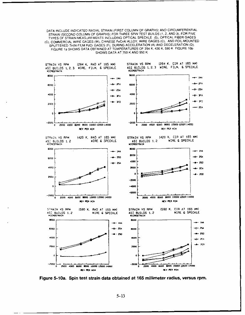
DATA INCLUDE INDICATED RADIAL STRAIN (FIRST COLUMN OF GRAPHS) AND CIRCUMFERENTIALSTRAIN (SECOND COLUMN OF GRAPHS) FOR THREE SPIN TEST BUILDS (1, 2, AND 3). FOR FIVETYPES OF STRAIN MEASUREMENTS INCLUDING OPTICAL SPECKLE (S), OPTICAL FIBER GAGES

(C), COMMERCIAL WIRE GAGES (W). CHINESE FeCrAI ALLOY, WIRE GAGES (C), AND FOIL-MOUNTEDSPUTTERED THIN-FILM PdCr GAGES (F). DURING ACCELERATION (A) AND DECELERATION (D).

FIGURE 1la SHOWS DATA OBTAINED AT TEMPERATURES OF 294 K, 420 K. 590 K. FIGURE 1lObSHOWS DATA AT 755 K AND 950 K.

STRAIN VS PPM (294 K. RAD AT 165 MM) STRAIN VS RPM (294 K. CIR AT 165 MM)ASI BUILDS 1.,2. 3 WIRE. FILM. &SPECKLE AS! BUILDS 1. 2, 3 WIRE. FILM., SPECKLEMII16- STRAI N MICF10STRAIN

-0.- IWA --- IWA

0 0

2000 400000080010001-e-4000400

2000 8000

-2000 -2000,

0 2000 4000 6000 800 10000 12000 14000 0 2000 4000 6000 8000 10000 12000 14000

REY PR MIN REV PER MIN

STRAIN VS RPM (420 K. RAD AT 165 MM) STRAIN VS RPM (590 K. CIR AT 165 MM)

AS: BUILDS 1.2 WIRE SPECKLE ASI BUILDS 2.2 WIRE SPECKLEIICROSTfAIN MCOSTRA*N

8000 8000-a-INA -*- WA

6000 -- 2SA 000 --- S

a _S 40 -w- 250

000 2000 -i- CA

2000 0-4- 2co

?000 2000

020 0100 -4000

-20 0 200 400 6'0 Go 00012000 14000 0 2000 4000 8000' 8000 10000 12000 14000

REV ER "N RV PER~ MIN

FigrJ VS~a Pin test stai PDat obaeda 165 milimte radius, vesu rp 50 .C 15 M .

ASIBULD 12 IR SPCKE SIBULD 1. WR5-13EKL

STRAIN VS RPM (755 K. RAD AT 165 MM) STRAIN VS RPM (755 K. CIR AT 155 MM)

ASI BUILD 2 SPECKLE ASI BUILD 2 WIRE G SPECKLEMim"0S £ N

MICOSTRAIN

400-46- 22A 4000 -U 2SA

-6- 2w 00 -4w- 290

o o --- 2CD

-2000 -2000

0 2000 4000 0 8000 1000 12000 14000 0 2000 4000 6000 000 o000 12000 14000

WY PHM EV NIN

STRAIN VS RPM (950 K. RAD AT 165 MM) STRAIN VS RPM (g50 K. CIR AT 165 MM)

ASI BUILDS 2 SPECKLE ASI BUILDS 2 SPECKLEuMXICTRAXN MICRM0TRAIN

8000 0000- 4 -2A em8n

6000 -6000-E- 2S -- 290

4000 4000

2000 -2000

-4000 -4000

-6000 1000

0 2000 4000 60 60 0W 12000 14000 0 2000 4000 600 W 10000 12000 14000

V PE MIN AEV PER MIN

STRAIN VS RPM (FILMS. RAO AT 165 oM) STRAIN VS RPMi (FILMS. CIR AT 165 M)

ASI OLDS 2. 31 2945 420. 590. 755 K ASI BLS 2. 3; 294. 420. 590. 755 KMI CIOSTIAIN MICHOSIKAIN

"0 " 6000w

50000 - 3 28 500 3 nJ4

40000 -0-2 420 400 P 4;0

30<00- -- 3 420 30 --0-- 3 4?O

0 2W00 4000 6000 SM0 10000 32M0 14W0 0 000 4000 6W0 i00 10002000 40

Figure 5-10b.(:Conclusion of data at 165 millimeter radius.

5-14

DATA SHOWN INCLUDE INDICATED RADIAL STRAIN (FIRST COLUMN OF GRAPHS) AND CIRCUMFERENTIALSTRAIN (SECOND COLUMN OF GRAPHS) FOR THREE SPIN TEST BUILDS (1, 2, AND 3). FOR FIVETYPES OF STRAIN MEASUREMENTS INCLUDING OPTICAL SPECKLE (S), OPTICAL FIBER GAGES

(0), COMMERCIAL WIRE GAGES (W), CHINESE FeCrAI ALLOY WIRE GAGES (C). AND FOIL-MOUNTEDSPUTTERED THIN-FILM PdCr GAGES (F), DURING ACCELERATIONS (A) AND DECELERATIONS (D).

DIGURE 2a SHOWS DATA OBTAINED AT TEMPERATURES OF 294 IK, 420 K, 590 K. FIGURE 11 bSHOWS DATA AT 755 K AND 950 K.

STRAIN VS RPM (294 K, RAD AT 152 MM) STRAIN VS RPM (294 K. CIR AT 152 MM)ASI BUILDS 2. 3 WIRE. FILM. & SPECKLE ASI BUILDS 2.3 WIRE. FILM. & SPECKLENIZRCSTRAIN MINROSTRAIN

6000 w-r 2CA 2CA

6000 6w --2SA --e-- 254

4000I_ 40-W 2FA6- 2FA

32 D 000j -0- 3F A

"-2000 -2000 O+••

-4000 -4000

-ABCOU- -6000

0 -0 4000 6000 00 0000 12000 14000 0 2000 4000 6000 8000 10000 12000 14000REV PER WIN REV PER k:3

STRAIN VS RPM (420 K. RAD AT 152 MM) STRAIN VS RPM (420 K. CIR AT 152 MM)ASI BUILDS 2 WIRE & SPECKLE ASI BUILDS 2 WIRE C SPECKLE

MICADSTRAIN MICR&STRAIN

woo sm--,-2CA -4.- 2CA

000 000

4000 4000-e- 2548 S

NO2000 -- 5

0-0 _ __-2000 -2000

-4000 -4000

-6000 -6000

0 2000 40006000 0 10000 12000 14 0 2000 4000 6000 000 10000 12000 14000REV PER HIN REV PER WIN

STRAIN VS RPM (590 K. RAD AT 152 MM) STRAIN VS RPM (590 K. CIR AT 152 MM)ASI BUILDS 2 SPECKLE ASI BUILDS 2 WIRE & SPECKLE

WICROSIRAIN MICROSTRAIN

-f0- 2SA -- ?CA

6000 w 6000

00

-2-0- 20 -00

-4000 -4000

-20u -6000

0 000 400 8000 6000 10000 12000 14000 0 20 4000 6000 6000 10000 22000 14000

REV PER MIN REV PER MIN

Figure 5-11a. Spin test strain data obtained at 152 millimeter radius, versus r/min.

5-15

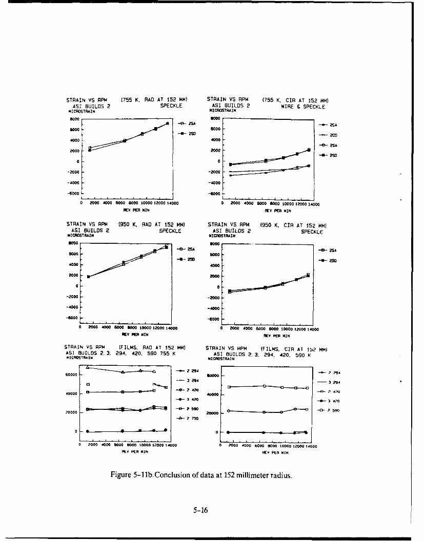
STRAIN VS RPM (755 K. RAD AT 152 MM) STRAIN VS RPM (755 K. CIR AT 152 MM)ASI BUILDS 2 SPECKLE ASI BUILDS 2 WIRE C SPECKLE

HICROSTRAIN NICSTRAIN

6000 3I000 ,

--w 2 p*-. 2CA6000 N 000,

4000 4000

2000 20900S2O2w

0 0

-2000 -2000

-4000 -4000

-6000

2000 4000 6000 6000 1000 12000 14000FIEV PE MIN REV PER MIN

STRAIN VS RPM (950 K. RAD AT 152 MM) STRAIN VS RPM (950 K. CIR AT 152 MM)ASI BUILDS 2 SPECKLE ASI BUILDS 2 SPECKLE

HICROSTRIN NICROSTRAIN6000 6000

•-6-- 2SO .-6- 2SA'6000 6000-0- 2w

4000 4000 -2

2000 -2000

0 0

-2000 -2000

-4000 -4000

-6000 -8000

0 200 4000 6000 1000 10000 12000 14000 2000 4000 6000 6000 10000 12000 24000

V PR HINREV PER MIN

STRAIN VS RPM (FILMS, RAO AT 152 MM) STRAIN VS 1PM (FILMS, CIR Al Ib? MM)AS] BUILDS 2. 3: 294. 420. 590 755 K ASI BUILDS . 3; 294. 420. 590 K

M1C11STRAIN NISTRAIN

60000 2 4 60000

- 3 294 - 294

-- _____________ -0 2 42'0 -0 .p 4;'o40000 2 0000

--0-- 3 420 -4-- 3 4?0

'0000 - 2 20000 P

-- 2755

0 L S

0 2000 4000 6000 9000 20000 12000 14000 0 ?000 4000 6000 3000 10000 12.000 14000REV PER MIN 14EV PER MIN

Figure 5-11b.Conclusion of data at 152 millimeter radius.

5-16

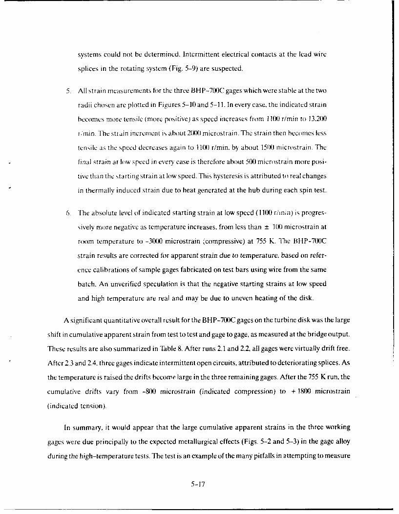
systems could not be determined. Intermittent electrical contacts at the lead wire

splices in the rotating system (Fig. 5-9) are suspected.

5. All strain measurements for the three BHP-700C gages which were stable at the two

radii chosen are plotted in Figures 5-10 and 5-11. In every case, the indicated strain

becomes more tensile (more positive) as speed increases from 1 1() r/min to 13,20X)

r, min. The strain increment is about 2(XX) microstrain. The strain then becomes less

tensile as the speed decreases again to 11(M r/min, by about 15(g) microstrain. The

final strain at low speed in every case is therefore about 500 microstrain more posi-

tive than the starting strain at low speed. This hysteresis is attributed to real changes

in thermally induced strain due to heat generated at the hub during each spin test.

6. The absolute level of indicated starting strain at low speed (1100 r/inin) is progres-

sively more negative as temperature increases, from less than ± 1(M microstrain at

room temperature to -3(M0 microstrain {compressive) at 755 K. The BHP-700C

strain results are corrected for apparent strain due to temperature, based on refer-

ence calibrations of sample gages fabricated on test bars using wire from the same

batch. An unverified speculation is that the negative starting strains at low speed

and high temperature are real and may be due to uneven heating of the disk.

A significant quantitative overall result for the BHP-700C gages on the turbine disk was the large

shift in cumulative apparent strain from test to test and gage to gage, as measured at the bridge output.

These results are also summarized in Table 8. After runs 2.1 and 2.2, all gages were virtually drift free.

After 2.3 and 2.4, three gages indicate intermittent open circuits, attributed to deteriorating splices. As

the temperature is raised the drifts become large in the three remaining gages. After the 755 K run, the

cumulative drifts vary from -80) microstrain (indicated compression) to + 1800 microstrain

(indicated tension).

In summary, it would appear that the large cumulative apparent strains in the three working

gages were due principally to the expected metallurgical effects (Figs. 5-2 and 5-3) in the gage alloy

during the high-temperature tests. The test is an example of the many pitfalls in attempting to measure

5-17

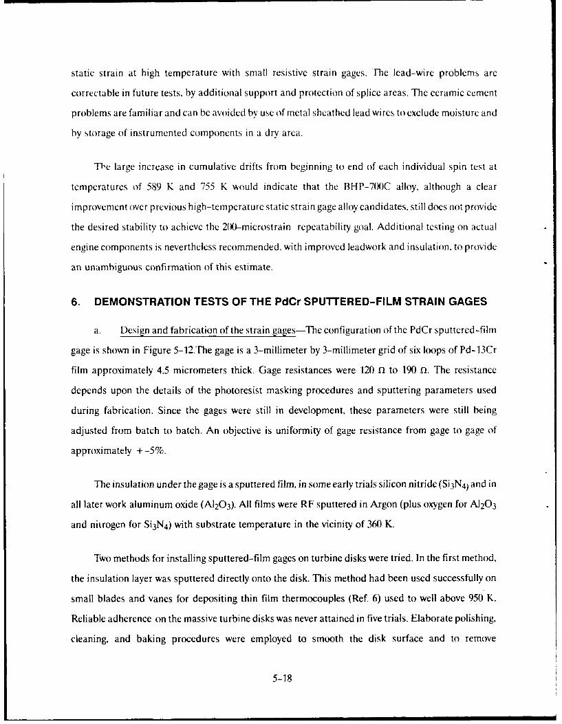
static strain at high temperature with small resistive strain gages. -he lead-wire problems are

correctable in future tests, by additional support and protection of splice areas. The ceramic cement

problems are familiar and can be avoided by use of metal sheathed lead wires to exclude moisture and

by storage of instrumented components in a dry area.

Th1e large increase in cumulative drifts from beginning to end of each individual spin test at

temperatures of 589 K and 755 K would indicate that the BHP-700C alloy, although a clear

improvement over previous high-temperature static strain gage alloy candidates, still does not provide

the desired stability to achieve the 2(X-microstrain repeatability goal. Additional testing on actual

engine components is nevertheless recommended, with improved leadwork and insulation, to provide

an unambiguous confirmation of this estimate.

6. DEMONSTRATION TESTS OF THE PdCr SPUTTERED-FILM STRAIN GAGES

a. Design and fabrication of the strain gages-The configuration of the PdCr sputtered-film

gage is shown in Figure 5-12.The gage is a 3-millimeter by 3-millimeter grid of six loops of Pd-13Cr

film approximately 4.5 micrometers thick. Gage resistances were 120 fl to 190 fl. The resistance

depends upon the details of the photoresist masking procedures and sputtering parameters used

during fabrication. Since the gages were still in development, these parameters were still being

adjusted from batch to batch. An objective is uniformity of gage resistance from gage to gage of

approximately + -5%.

The insulation under the gage is a sputtered film, in some early trials silicon nitride (Si 3 N 4 ) and in

all later work aluminum oxide (A120 3). All films were RF sputtered in Argon (plus oxygen for A120 3

and nitrogen for Si 3N4) with substrate temperature in the vicinity of 360 K.

Two methods for installing sputtered-film gages on turbine disks were tried. In the first method,

the insulation layer was sputtered directly onto the disk. This method had been used successfully on

small blades and vanes for depositing thin film thermocouples (Ref. 6) used to well above 950 K.

Reliable adherence on the massive turbine disks was never attained in five trials. Elaborate polishing,

cleaning, and baking procedures were employed to smooth the disk surface and to remove

5-18

a|

Figure 5-12. Four thin-film gages mounted on a test bar for gage factor testing.

contamination before sputtering. Atomic cleanliness was verified using the deionized water "break"

test in which complete wetting assures the absence of organic contaminants. The sputtered layers

eventually delaminated in every case (sometimes only after temperature cycling). The existence of

organic contamination was then verified under the delaminated layers by the water break test. The

conclusion was that these massive engine components could probably never be completely free from

contaminants emerging from deep below the surface.

5-19

The second method was sputtering the insulation layer and gages on transferable weldable thin

(127 micrometer) metal foils of polished and sputter -etched Hastelloy X. This method was eventually

successful and was used throughout the present program. After completion of the sputtered film gage,

the foil was spot welded to the turbine disk.

The sputtered gage patterti included wide lead films of PdCr extending to a location convenient

for attaching lead wires by parallel-gap capacitive discharge welding. The lead wires were then

overcoated with ceramic cement for protection from oxidation and erosion. The strain gages were not

coated with ceramic cement. A sputtered overcoat of A120 3 was applied to one final batch of gages in

this program to retard oxidation of the PdCr gage. Performance with and without the sputtered

overcoat was thus documented.

Before the beginning of the program, preliminary in-house experiments had been carried out to

measure the gage factor of these sputtered-film foil-mounted gages and to verify that repeatable and

linear strain transfer could be achieved with foil-mounted gages. Figure 5-12 shows four

sputtered-film gages on a foil welded to a Hastelloy X test bar 114 in thick for room-temperature

testing and Figure 5-13 shows the results. The gages in this preliminary test were of an experimental

FeCrAI alloy and the insulation under the gages was Si 3N4.Good strain transfer to the gages sputtered

on the foil is demonstrated in Figure 5-13 in tension ( + ) and in compression (-), for both longitudinal

and transverse gages. The data symbols are the gage numbers.

b. Results of preliminary static tests: Ferris wheel-In the Ferris wheel test rig, a turbine disk

is radially loaded through rods attached to each turbine blade dovetail. The disk is heated by induction

heaters placed nearby and is oscillated slowly back and forth through less than 1800 to promote

uniform heati- g. The rig, located at Pratt & Whitney, is shown in Figure 5-14, with the disk used in the

present program installed. The testing is in air at sea-level pressure.

In preparing for the Ferris wheel test, preliminary sets of six sputtered-film gages were fabricated

on several foils, some using the Si3N4 sputtered insulation and some using the A120 3. The Si 3N4 is a

poorer match in temperature coefficient of linear expansion with the foil material, and as a result

cventual delamination would be expected at a lower temperature. This was verified when the Si 3N4

5-20

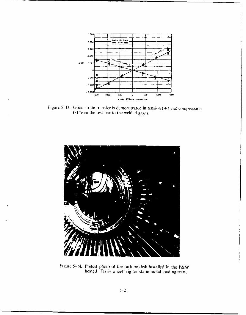
004 FO.AJ (ON OL) -

THU IS APR 15....__

0003 -4--

0002 1

AR/R 0001 IVE; GAGE

0[0001 a

-0003-1500 1000 -500 0 500 1000 1500

AXIAL STRAIN, mcrostrain

Figure 5-13. Good strain transfer is demonstrated in tension (+) and compression(-) from the test bar to the weld d gages.

Figure 5-14. Pretest photo of the turbine disk installed in the P&Wheated "Ferris wheel" rig for static radial loading tests.

5-21

Catast rophically dclami natedCL from[1 one foil (Hg. 5-15S) whaico coo diig fro~m 9501 K during temperat ure

cycling inI bentch test,;. No delamination of the A12()3 films occurred alter many cycles.

46

laigurc 5- 15. An example of catastrophic delamination of the Si 3N4 sputteredinsulation at 9501 K during a preliminary trial of the foil-mounted gagesoin a turhine disk.

Figurc 5- 16 Is a view of the final Installation of the PdCr sputtered-film foil-mounted gages on

the turbine disk for the Ferris wheel test. 'Ilree gages were installed, including a radial gage at a radius

oif 141) millimecters ( I R) and a radial gage and a tangential gage at a radius of 165 millimeters (2R and

.11). The gages are Ud-130', 4.5 micrometers thick oin A1203 insulation 4 micrometers thick, all

sputtered on a I lastelloy X foil 127 micrometers thick that is welded to the disk as shown. There was no

overcoait protection oin the Pd( 4 gages.

Figure 5- 17 s~how,, mcasured strain verstis Ferris wheel applied radial load at room temperature

fr gage 2R. Repcitahility Is good for 1neit~asling and decreasing load. Maximum mecasured strain Is

f-iicure 5-16. Pretest photo bMOrN 950 K static Ferris wheel test.

1 2

0 9-

INDICATED

0 4 0 INCREASING

o 3 D ECREASING.

RO TEMPERATURE

4 6LOAD POUNDS IllOU~ands

1iIgurc I~ %:le-urcd sta;vs Verris %ho-cI radial load.

5-23

about 1200 microstrain. The nonlinearity at highest strain has not been explained. During the course of

the high-temperature testing the scatter in measured strains was thousands of microstrain.

Figure 5-18 is a post-test view after the 950 K testing in the Ferris wheel rig. The sputtered-film

gages appear to be in good condition. There is dark discoloration suggesting that considerable

oxidation has occurred. There is no delamination. There is damage to the grid of gage IR apparently

due to impact from debris.

One of the three gages was functioning at the end of the program (2R), one was open at the lead

wire connection to the lead film (3T), and the third was open at the gage grid (1R).

The most significant quantitative result for this initial set of PdCr gages was the change in

resistance of the gage and the change in leakage to ground over the course of the testing. Table 9 lists

the pretest and post-test measurements. Measured gage resistances at start were 124, 148, 167 ohms,

and all resistances to ground were over 40 megohms. Measured gage grid resistances at finish were

open, 155, and 197 ohms and resistances to ground were 1000 to 6000 ohms.

The low resistances to ground would reduce the measured gage resistances by 1.1% to 4.4%. If

moderate oxidation of the PdCr alloy gages had occurred, it would be expected that the gage resistance

would be lower yet, due to the selective oxidation of the chromium, moving the alloy toward pure

palladium (lower resistivity). This effect has been observed in controlled moderate oxidation tests of

sputtered films of PdCr. However, in the present test, the actual post-test measured gage resistances

for the two intact gage grids (Table 9) were higher than the pretest resistances (by 3.9% and 13.2%). It is

concluded that the oxidation was so extensive that the chromium oxide scale extended far into the

PdCr film and isolated some of the palladium on the external surface of the oxide scale. This

phenomenon has been observed in oxidation experiments, although data are not available yet to

unambiguously define an increase in sample resistance from this effect.

The post-test observed leakage to ground could, in small part, be due to absorption of moisture

in the ceramic cement on the lead wires at room temperature after the end of testing, but since the

post-test measurements were made within I day of the end of this test, this contribution is believed

5-24

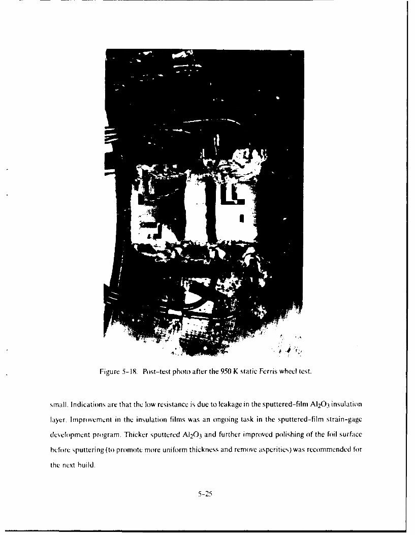
Figure 5-18. Post-test photo after the 950 K static Ferris wheel test.

small. Indications are that the low resistance is due to leakage in the sputtered-film A120 3 insulation

layer. Improvement in the insulation films was an ongoing task in the sputtered-film strain-gage

development program. Thicker sputtered A120 3 and further improved polishing of the foil surface

before sputtering (to promote more uniform thickness and remove asperities)was recommended for

the next build.

5-25

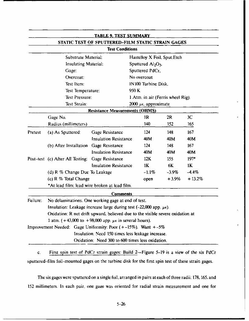
TABLE 9. TEST SUMMARY

STATIC TEST OF SPUTTERED-FILM STATIC STRAIN GAGESTest Conditions

Substrate Material: Hastelloy X Foil, Sput.EtchInsulating Material: Sputtered A120 3,

Gage: Sputtered PdCr,

Overcoat: No overcoat

Test Item: IN100 Turbine Disk,

Test Temperature: 950 K

Test Pressure: I Atm. in air (Ferris wheel Rig).

Test Strain: 2000 gE, approximate

Resistance Measurements (OHMS)

Gage No. 1R 2R 3C

Radius (millimeters) 140 152 165

Pretest (a) As Sputtered: Gage Resistance 124 148 167

Insulation Resistance 40M 40M 40M

(b) After Installation Gage Resistance 124 148 167Insulation Resistance 40M 40M 40M

Post-test (c) After All Testing: Gage Resistance 12K 155 197*

Insulation Resistance 1K 6K 1K

(d) R % Change Due To Leakage -1.1% -3.9% -4.4%

(e) R % Total Change open +3.9% + 13.2%*At lead film: lead wire broken at lead film.

CommentsFailure: No delaminations. One working gage at end of test.

Insulation: Leakage increase large during test (-22,000 app. liE).

Oxidation: R net drift upward, believed due to the visible severe oxidation at

I atm. ( + 43,000 to + 98,000 app. AiE in several hours).

Improvement Needed: Gage Uniformity: Poor (+ -15%). Want + -5%

Insulation: Need 150 times less leakage increase.

Oxidation: Need 300 to 600 times less oxidation.

c. First spin test of PdCr strain gages: Build 2-Figure 5-19 is a view of the six PdCr

sputtered-film foil-mounted gages on the turbine disk for the first spin test of these strain gages.

The six gages were sputtered on a single foil, arranged in pairs at each of three radii: 178, 165. and

152 millimeters. In each pair, one gage was oriented for radial strain measurement and one for

5-26

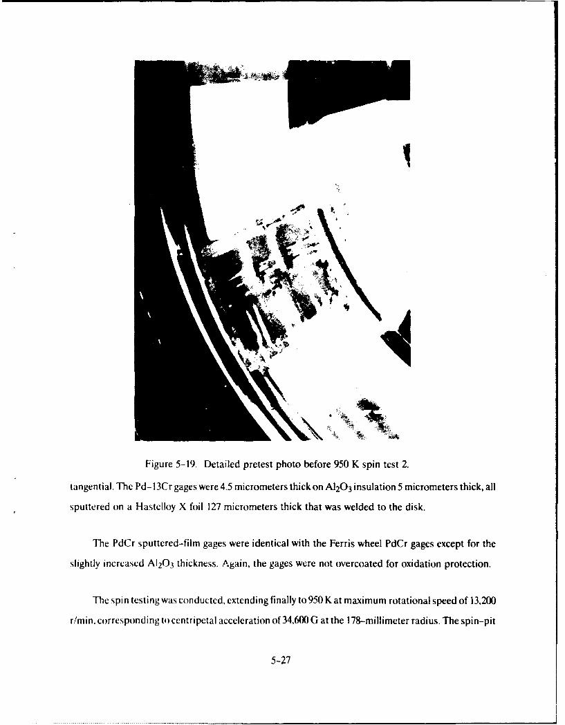
II

Figure 5-19. Detailed pretest photo before 950 K spin test 2.

tangential. The Pd-13Cr gages were 4.5 micrometers thick on A120 3 insulation 5 micrometers thick, all

sputtered on a Hastelloy X foil 127 micrometers thick that was welded to the disk.

The PdCr sputtered-film gages were identical with the Ferris wheel PdCr gages except for the

slightly increased A120 3 thickness. Again, the gages were not overcoated for oxidation protection.

The spin testing was conducted, extending finally to 950 K at maximum rotational speed of 13,200

r/min, corresponding to centripetal acceleration of 34,600 G at the 178-millimeter radius. The spin-pit

5-27

operating pressure was approximately O.00)1 atm. At the end of this test, as previously mentioned in

the discussion of the BHP-700C gages, the disk bore became overheated resulting in melting ,f

leadwire splices.

Strain readings from the PdCr gages were recorded throughout the spin program and are

discussed at the end of this section.

Figure 5-20 is a post-test view. The sputtered-film gages appear to be in good condition. Slight

discoloration of the PdCr films suggests moderate oxidation had occurred. There is no delamination.

Figure 5-20. Post-test photo after the 950 K spin test 2.

Pretest and post-test measurements of gage resistance and resistance to ground are listed in

Table 10. These measurements are among the most significant results for the sputtered-film gages in

this test.

In the table, three sets of pretest measurements are presented. The first set shows that the range

of gage resistance as sputtered was 158 to 200 fl, still about three times the desired uniformity of

+ -5%, showing that resistance to ground as sputtered was low (8 to 1300 f)). We found by probing that

the leakage was at discrete point locations all of which were in the lead film area. To rupture the leakage

5-28

paths 30 V dc was applied at the identified locations. The second set of readings shows that this

procedure was successful in increasing the resistance to ground to 40 ml! for four gages. These four

gages were connected to the data system and used in the spin testing. This procedure also resulted in

higher measured gage readings for some gages, as would be expected by the elimination of leakage

paths. In other cases the measured gage resistance was unaffected, as would be expected if all the

leakage paths for that gage were in one lead film. The third set of pretest readings shows that a pretest

temperature cycle carried out to verify the adherence and stability of the films, resulted in a few ohms

reduction in each gage resistance, probably because of preferential oxidation of the chromium in the

PdCr alloy.

The post-test measurements in Table 10 show that the measured gage resistances all decreased,

by amounts from 8.5% to 21.0%. Part of the measured decrease is due to shunting as a result of the

decrease in measured resistance to ground to approximately 200 t for each gage. As previously noted

tor this build, these particular post-test leakage measurements are believed to be due in significant

part to post-test moisture absorption in the ceramic cement. The calculated downward drift in actual

gage resistance, after taking into account the shunting, is the equivalent of -37,000 to -104,000

apparent microstrain (based on a gage factor of 1.8 for the PdCr alloy from Reference 2). This drift

occurred during the testing at 950 K, driving the data acquisition system off scale and resulting in no

strain measurements at temperatures above 755 K. The drift in the downward direction of this

magnitude is entirely compatible with the effects of moderate oxidation seen in other testing (Ref.2)

and verifies that provision of an oxidation-protection overcoat is a first priority for the further testing

of PdCr gages, even in a vacuum spin rig.

Rotating strain data obtained with the foil-mounted sputtered thin-film PdCr gages is compared

in Figures 5-10a and 10b and Figures 5-11a and llb with the data obtained with the other strain

measuring techniques, including optical speckle, optical dual-core fiber optic gages, commercial wire

gages, and Chinese BHP-700C FeCrAI alloy wire gages. Data are presented at the only two radii (165

millimeters and 152 millimeters) at which all five types of data were acquired.

5-29

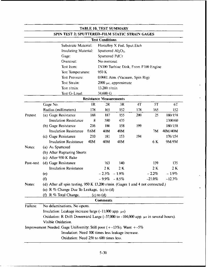
TABLE 10. TEST SUMMARY

SPIN TEST 2; SPUTTERED-FILM STATIC STRAIN GAGESTest Conditions

Substrate Material: Hastelloy X Foil, Sput.Etch

Insulating Material: Sputtered A120 3,Gage: Sputtered PdCrOvercoat: No overcoat

Test Item: INI0) Turbine Disk, From FIN) EngineTest Temperature: 950 K

Test Pressure: 0.(001 Atm. (Vacuum, Spin Rig)

Test Strain: 20W IE, approximateTest r/min: 13,200 r/minTest G-Load: 34.600 G

Resistance Measurements

Gage No. IR 2R 3R 4T 5T 6TRadius (millimeters) 178 165 152 178 165 152

Pretest (a) Gage Resistance 188 187 155 200 25 180/158

Insulation Resistance 8 580 435 13W1/60(b) Gage Resistance 216 186 158 199 180/158

Insulation Resistance 0.6M 40M 40M 7M 40M/40M

(c) Gage Resistance 210 181 153 194 176/154Insulation Resistance 40M 40M 40M 6 K 9M/9M

Notes: (a) As Sputtered

(b) After Rupturing Shorts

(c) After 950 K BakePost-test (d) Gage Resistance 163 140 139 135

Insulation Resistance 2 K 2 K 2 K 2 K

(e) - 2.3% - 1.9% - 2.2% - 1.9%

(f) - 9.9% - 8.5% -21.0% -12.3%Notes: (d) After all spin testing, 950 K 13,200 r/min. (Gages 1 and 4 not connected.)

(e) R % Change Due To Leakage, (c) to (d)(f) R % Total Change. (c) to (d)

CommentsFailure: No delaminations, No opens.

Insulation: Leakage increase large (-11,000 app. AE)

Oxidation: R Drift Downward Large (-37,000 to -104,000 app. IxE in several hours).

Visible Oxidation.Improvement Needed: Gage Uniformity: Still poor (+ -13%). Want + -5%

Insulation: Need 100 times less leakage increase.

Oxidation: Need 250 to 600 times less.

5-30

An overall summary and intercomparison of all strain results in Figures 5-10a and 10b and

Figures 5-11a and 1 lb is presented in the executive overview section (Volume I). Notable details of the

results obtained with the foil-mounted sputtered PdCr thin-film gages in Build 2 are presented here as

follows (still referring to Figures 5-10a and 10b and Figures 5-1la and lIb:

1. Radial and circumferential strain measurements were obtained with the Build 2

foil-mounted sputtered PdCr thin-film gages at both radii, at the five rotational

speeds during the acceleration at 294 K (the rig was shut down directly after the ac-

celeration at 294 K, without pausing to acquire data during deceleration). In addi-

tion, data were acquired in almost every case at all speeds during both acceleration

and deceleration at each of four higher temperatures: 420 K. 590 K, 755 K. The

exceptions were radial strain at 165 mm at 590 K and circumferential strain at 152

mm at 755 K. In these two cases, signal was lost during the run but recovered later.

Finally, thin-film gage data were also acquired during the spin test at 950 K, but

these gage output readings were so large due to temperature effects that the data

system was saturated (off scale) and no strain information could be derived from

the readings.

2. At room temperature, the Build 2 thin-film indicated strains (Figs. 5-10 and 5-11)

are near zero at lowest speed and become more tensile (more positive) as speed in-

creases from 1100 r/min to 13,200 r/min. The strain increment is about 2000 micro-

strain. In this room-temperature spin test, the absolute level and the strain

increment with increasing speed are generally in good agreement with most of the

other strain measurements (speckle, dual-core fiber, commercial wire gage,

BHP-7(X)C gage), to about ± 300 microstrain. For unexplained reasons, one thin-

film gage (radial at 152 mm) indicates a smaller positive increment by about 500

microstrain, than all others.

3. At the elevated temperatures, the apparent strain due to temperature for the thin-

film gages dominates the indicated strain readings. For this reason, the indicated

5-31

strains for the thin-film gages at elevated temperatures are plotted separately at the

bottom of Figure 5-10b and Figure 5-1lb. The indicated strain increases by about

100 microstrain per Kelvin for each of the four thin-film gages. This is in the range

expected for these gages without temperature compensation. (The temperature co-

efficient of resistance is about 180 x 10-6 K- 1 and the gage factor is about 1.8. The

predicted apparent strain is therefore about 180/1.8 = 100 micron strain per Kel-

vin.) No attempt was made to correct the readings for these large temperature ef-

fects. Since the local temperature of the disk is not known to within about 20 K, then

the correction uncertainty would be on the order of 200) microstrain. In the continu-

ing development program, self temperature compensation is to be added to the

PdCr gage systems by adding a high-tcr metal element in an adjacent arm of the

bridge circuit.

d. Second spin test of PdCr strain gages: Build 3-Figure 5-21 is a view of the six PdCr strain

gages of Build 3 after the foil was spot-welded to the disk and leadwork was attached, and before

installation of thermocouples and final cement overcoating of leadwork. This view shows clearly how

the rows of spot welds are placed within 1.5 millimeters from the gage on all four sides.

Figures 5-22 is a general view of the completed installation. The six gages were sputtered on a

single foil, in pairs at each of three radii: 165, 152, and 140 millimeters. In each pair one gage was

oriented for radial strain measurement and one for tangential. The PdCr gages were 4.5 micrometers

thick on A120 3 insulation 5.0 micrometers thick, all sputtered on a Hastelloy X foil 127 micrometers

thick that was welded to the disk.

The sputtered-film gages were identical with the Build 2 PdCr gages except that more elaborate

masking was used to improve uniformity of gages, extra care was taken in polishing the foil before

sputtering insulation, to improve integrity of the sputtered insulation layer, and, most important, an

oxidation-protection overcoat of A120 3 3 micrometers thick was sputtered on the PdCr gages.

5-32

Figure 5-21. Detailed pretest photo before 950 K spin test 3, before cementing of leadwires.

The spin testing extended to 950 K at 13,200 r/min, corresponding to centripetal acceleration of

32.1(9) G at the 165 millimeter in radius and to predicted strains of about 2000 microstrain. The

,pin-pit opcrating pressure was approximately 0.0001 atmospheres.

At one point early in this test, after room-temperature runs to maximum speed but before

high-temperature runs. a seal rub occurred in the rig bore resulting in destruction of leadwork and

hombardment of the PdCr .puttered-film gages with hot debris. The gages were found to be

undamaged and the gage resistances not significantly changed, and resistance to ground unchanged

5-33

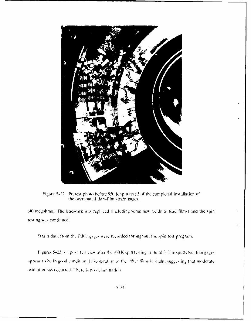
Figure 5-22. Prctest photo) before 950) K spin test 3 of the completed installation ofthe overcoated thin-film strain gages

(40 inegohms). The leadwork was recplaced (incl'jdiniz some new welds to) lead films) and the spin

testing was continued.

L train data froim the PdCr 2Aicsere recorded throughout the spin tes~t pro~gram.

Figures 5-23 is a powt-tce t vicA aftcr the 9q() K spin testing in Build 3~ -The sputtered-filni gages

aippear to he in goo)d condition. I i ri]( M !he ld(.'r turnUs i, ,,light. suggesting that moderate

o)xidatit n has occurred. 1-hero is, r'i) dclaiinationl.

5-314

N

Figure 5-23. Post-test detailed view of the ovwrcoated thin-film strain gages alter950 K spin test 3.

Pretest and post-test measurements of gage resistance and resistance to ground are listed in

Tahle 11. These rreasurements are again among the most significant results. In the tab! .- four sets ot

pretest mcasurt.mnents are presented. These measurements show excellent uniformity gage to gage.

high resistance to gtround, and little effect of the installation procedures.

The first set sho~ks that the range of gage resistance as sputtered was 151 to 163 ohmis (range of

+ -6r; ), nearly within the de.~ired uniformnity of + -5%, and shows that resistance to ground ats

sputtered was high (40 megohms) except for one gage (7000 f). We found by probing that the leakage

for this gage was at one discrete point in one lead film. To rupture this leakage path 30 V dc was applied

at the identified location. The second set of readings shows that this procedure successfully increased

the resistance to ground to 40 megohms. The third set of pretest readings was taken after welding the

foil to the disk, and the fourth set after installing leadwork and after a 600 K pretest temperature cycle

to cure cements on leadwork. Resistance to ground remains at 40 megohms for all gages. Measured

gage resistances all decreased by 4 + -1 ohm. This decrease is apparently due to aging, and some

oxidation, during the temperature cycle to 600 K. The repeatability of the ohmmeter used was + -0.2

ohm. The effect of temperature on the resistivity of PdCr would change the gage resistance by one ohm

only if the temperature change were about 37 K. Therefore small variations in room temperature from

reading to reading would not significantly alter the values in this table. All six gages were then

connected to the data system and used in the spin testing.

Two sets of post-test measurements are presented in Table 11. The first set was obtained after the

interruption in testing to repair the damage resulting from the rig seal rub. The second was obtained

after all testing.

The first set shows that gage resistances are virtually unchanged and that resistance to ground

remains above 40 megohms for all gages.

The final set of post-test measurements (Table 11) shows that after all testing, three gages are

open-circuited and the other three have drifted downward in resistance by an additional 5 n to 6 fn

(about 4%).

The resistance to ground has also decreased to 15,000 to 45,000 ohms, equivalent to an apparent

strain offset of about -1300 microstrain, or a 0.2% decrease in measured gage tesistance. In addition,

discrete short circuits to ground have developed in the lead films, at one end only, in three gages.

5-36

TABLE 11. TEST SUMMARY

SPIN TEST 3; SPUTTERED-FILM STATIC STRAIN GAGESGage Construction

Substrate Material: Hastelloy X Foil, Sput Etch

Insulating Material: Sputtered A120 3

Gage: Sputtered PdCr

( hercoat: Sputtered Al20 3

Test Conditions

Test Item: INI(N) Turbine Disk, From F100 Engine

-I& t -cmperature: 950 K

Test Pressure: 0.(10)] Atm. (Vacuum, Spin Rig)

Test Strain: 2(9X) LE, approximate

lest r/min: 13,2(X) r/min

lest G-Load: 32.1(X)

Pretest Resistance Measurements (OHMS)

G Gage No, IC 2R 3C 4R 5C 6R

Radius (:-illimeters) 165 165 152 152 140 140

Gage Resistance (a) 154 152 154 151 152 163

(b) 151

(c) 148 149 146 150 148 156

(d) 150 148 150 148 148 158

Insulation Resistance (a) 40M 40M 40M 7 K 40M 40M

(b) 40M

(c) 40M 40M 40M 40M 40M 40M

(d) 40M 40M 40M 40M 40M 40M

Notes: (a) As Sputtered

(b) After Rupturing Short

(c) After Welding Foil to Disk

(d) After Splicing Sheathed Lead and 600 K Bake

5-37

TABLE 11. TEST SUMMARY (CONTINUED)

SPIN TEST 3; SPUTTERED-FILM STATIC STRAIN GAGES

Post-Test Resistance Measurements (OHMS)

G Gage No. 1C 2R 3C 4R 5C 6R

Radius (millimeters) 165 165 152 152 140 140

Gage Resistance (e) 148 146 149 146 145 156

(f) 144 0.IM 145 142 3.3 K 66 K

Insulation Resistance (e) 40M 40M 40M 40M 40M 40M

(f) 1 40 K 45 K 15 K 3 1

Notes: (e) After 1st spin, 420 K 13200 r/min, and rig repair.

() After final spin, 950 K 11400 r/min.

Resistance Change Due To Leakage (%) -0.2% -0.1% -0.1% -0.2% -4.4% -0.3%

Total Resistance Change (%) (d to f) -4.0% open -3.3% -4.0% open open

Comments

Failure Comments: No delaminations, 3 opens, 3 good gages.

Insulation: Leakage increase large during test (-1300 microstrain)

Oxidation: 2 to 5 times reduced drift in 3 good gages (-18000 to -21000

app. gtE in several hours).

Improvement Needed: Gage Uniformity: Good (+ -6%); Close to + -5% target.

Insulation: Need 10 times less leakage change, and eliminate point shorts

to ground. Oxidation: Need 120 times less.

The calculated downward drift in actual gage resistance, after considering the shunting due to

insulation leakage, is the equivalent of -18,000 to -21,000 apparent microstrain (based on a gage factor

of 1.8 for the PdCr alloy from Reference 2). This drift is two to five times less than for the unovercoated

PdCr gages of Build 2, but is still far in excess of the goal of 200 microstrain uncertainty in strain

measurement.

The gage resistance drift in the downward direction indicates that the oxidation protection for

the PdCr gage must be improved by another factor of about 120. Increasing the thickness of both the

5-38

PdCr and the A120 3 coating, adding a metal top layer as an oxygen barrier, and hot sputtering of the

A120 3 to avoid entrained gases are avenues being explored.

Finally, the insulation layer under miese gages clearly requires turther improvement. For

example, measured resistance to ground of more 187,00 f) at each end of the gage at all temperatures

up to the maximum of interest will be required to keep apparent strain due to leakage below 2()

microstrain in a 151) ohm gage. In the ongoing development program, the mechanisms of insulation

layer leakage are being investigated.

Build 3 rotating strain data obtained with the foil-mounted sputtered thin-film PdCr gages is

compared in Figures 5-10a and 10b and Figures 5-11a and lib with the data obtained with the other

strain measuring techniques, including optical speckle, optical dual-core fiber optic gages. Data are

presented at the only two radii (165 millimeters and 152 millimeters) at which ai five types of data were

acquired.

An overall summary and intercomparison of all strain results in Figures 5-10a and 10b and

Figures 5-1 la and 1 lb is presented in the executive overview section. Notable details of the results

obtained with the foil-mounted sputtered PdCr thin-film gages in Builds 2 and 3 are presented here as

follows (still referring to Figures 5-10a and 10b and Figures 5-11a and lb):

I. Radial and circumferential strain measurements were obtained with the Build 3

foil-mounted sputtered PdCr thin-film gages at both radii, at the five rotational

speeds during the acceleration and deceleration at both 294 K and at 420 K. Based

on the experience of Build 2, in which it was confirmed that the apparent strain due

to temperature was about 100 microstrain per Kelvin for the uncompensated thin-

film gages, an attempt was made to keep the strain readings within the range of the

data system at each temperature by rezeroing the thin-film strain gage bridge out-

put voltage at temperature. This procedure worked at 420 K as described below, but

not enough range of adjustment was available for the higher temperatures. As a

result, no strain information could be derived from the readings at temperatures

above 420 K.

5-39

2. Both at room temperature and at 420 K, the Build 3 strains measured with the thin-

film gages (Figs. 5-10 and 5-11) are near zero at lowest speed and become more ten-

sile (more positive) as speed increases from 1100 r/min to 13,200 r/min, and then

return to near zero as speed decreases to 1100 r/min. For one of the four thin-film

gages (165 mm, radial) the strain increment with increasing speed is about 2000

microstrain, in good agreement with most of the other strain measurements

(speckle, dual-core fiber, commercial wire gage, BHP-700C gage). For unexplained

reasons, the other three thin-film gages indicates a smaller positive increment by

about 1000 microstrain.

7. CONCLUDING REMARKS

The strain gage testing on rotating turbine disks in a spin rig to 950 K demonstrated some

progress toward overcoming the historical problems which have prevented attaining useful static

strain measurements above 660 K with small high-temperature resistance strain gages. The long-term

goal of uncertainty below 200 microstrain has not yet been approached. Uncertainty is still in the area

of 2000 to 20.000 microstrain at high temperatures.

The gages of the FeCrAI alloy developed in China were durable and demonstrated less

metallurgical drift than any previously reported FeCrAI alloy. The gages of the PdCr alloy under

development in sputtered-film form at United Technologies Research Center under NASA contract

were also durable, and showed improvement from build to build in oxidation resistance and insulation

resistance to ground.

The FeCrA! alloy wide gages are more durable because of the use of conventional leadwires and

insulation. The PdCr alloy film gages have better accuracy, when they survive, because of their

resistance stability.

Fvrther development of the PdCr alloy gage system is recommended because the alloy itself is

metallurgically stable. This gage system requires improved oxidation protection and improved

resistance to ground. In final developed form, temperature compensation will be required because of

the higher tcr of this alloy.

5-40

8. ACKNOWLEDGEMENTS

D.R. Englund and WS. Kim at NASA Lewis Research Center encouraged applying the PdCr

technology being developed under NASA contract at United Technologies Research Center (UTRC).

Dr. C.O Hulse, the UTRC Program Manager for the NASA contract, provided invaluable advice and

support.

9. BIBLIOGRAPHY

Stange WA., Advanced Techniques For Measurement Of Strain And Temperature In A Turbine En-

gine, AIAA Paper No. 83-1296. AIAA/ASME/SAE 19th Joint Propulsion Conference, Seattle,

Washington, June 27-29. 1983.

Hulse, C.O., Bailey, R.S., Grant, H.P., Przybvszewski, J.S.; High Temperature Static Strain Gage Devel-

opment Contract, Interim Report, NASA CR-180811, Contract NAS3-23722, 1987.

Wu, TT, Ma. L.C., Zhao, L.B., Development Of Temperature Compensated Resistance Strain Gages

For Use 16 74) C, Experimental Mechanics 21(3), 117-123, March 1981.

Wu, TT., Ma, L.C., Comparison Of Characteristics Of Our Temperature-Compensated Resistance

Strain Gages For Use To 7(0) C and 800 C, Fourth Annual Hostile Environments And High Tem-

perature Measurements Conference Proceedings, Society For Experimental Mechanics, 1987,

p. 30-34.

Fulton. G.B., Advanced Structural Instrumentation Test Facility AIAA Paper No. 88-3145, AIAAI

ASME/SAE/ASEE 24th Joint Propulsion Conference, Boston, Mass., July 11-13, 1988.

Grant, H.P, Przybyszewski, J.S., Anderson, WL., Claing, R.G., Thin Film Strain Gage Development

Program, Final Report, NASA CR-174707, 1983

Grant, H.P, Anderson, WL., Prxybyszewski, J.S., Rotating Tests of Advanced High Temperature Wire

and Thin-Film Strain Gages, AIAA Paper No. 88-3145, 24th Joint Propulsion Conference Bos-

ton, Mass. July 11-13, 1988.

5-41

VI. TEST FACILITY

1. ABSTRACT

The objective of this program performed under Air Force Contract F33615-83-C-2330 was to

demonstrate the accuracy and durability of advanced steady state strain and temperature sensors in

an environment typical of advanced gas turbine engines. A first stage turbine disk which operates at

speeds up to 13200 r/min and temperatures of 950 K was selected as the test vehicle. Simulated engine

operating conditions were achieved in the United Technologies Research Center's spin facility. This rig

was designed for structural dynamic measurements and evaluation of a wide range of rotating

components. This section of the report describes the spin rig configuration, drive system test rotor and

support equipment. Included is a discussion of the modifications made to achieve high temperature,

and the data acquisition system and test procedure.

2. INTRODUCTION

The high speed spin rig at UTRC is built for structural dynamic testing of a wide range of rotating

components. Turbomachinery components, propellers and helicopter blades were given foremost

consideration during design but other applications such as labyrinth seal tests were also planned.

Since it is not designed for failure testing, it was constructed above ground with the drive system and

instrumentation located below the vacuum chamber thus leaving the top surface completely

unobstructed and available for various optical measurement techniques. Figure 6--1 shows an overall

view of the 3.04 m diameter by 0.91 m high vacuum chamber and pump system. Test experience to date,

includes speeds up to 13,200 r/min, but with appropriate modifications, operation up to 30,000 r/min is

possible. The test chamber is maintained at vacuum conditions to minimize drive power requirements,

to evaluate structural properties of blades without aerodynamic effects, and to reduce the explosion

hazard resulting from entrapped oil vapor or explosive dust generated by accidental rotor failure. For

the Advanced Structural Instrumentation testing, capability was added to the rig to heat the test piece

up to 950 K, which necessitated heat shielding and cooling systems to confine the heat to the test

chamber itself. A rotor assembly consisting of disk, blades, and side plates from an aircraft first stage

high pressure turbine is used as the test piece throughout the program. Additionally, the number and

6-1

variety of sensors evaluated required that the tests be carried out in a series of rig builds, a build

consisting of a group of sensors mounted on a disk and tested over the complete operating envelope.

As familiarity was gained with the thermal response of the rig, it was feasible to make modifications

between builds to correct or modify operating characteristics.

V V

q '4

Figure 6-1. Overall view of UTRC spin rig.

The sections below will describe the construction of the rig in more detail including the drive and

control system as well as the slip ring and data acquisition components. The heating system and

development (it heat shielding and cooling components will also be described.

3. SPIN RIG DESCRIPTION

Ilhe acuUrn chamhicr is a cylindrical steel weldment of 19 mm thick plate 3 m in diameter and

191 in high in l-iurc 6-2. 1 he bottom and top cover plates are 51 mm and 76 mm thick respectively.

The comptctc drive sVstuLT coMpriing spindle, air turbine and slip ring, is mounted on the vacuum

6-2

chamber bottom plate. Speckle Photogrammetry, a noncontacting optical displacement measuring

technique, has been used for all the builds as a strain reference. The characteristics of the telecentric

lens used for the speckle photogrammetry measurements in these tests, required that the plane of the

test rotor be a specified distance from the focal plane of the lens. To achieve this distance, the complete

drive system is raised by means of the spool piece shown in Figure 6-2. An added benefit derived from

the use of the spool piece (not generally used for other tests) is that it gives additional room under the

rig for a second 48-channel slip ring. A continuous 76-mm-thick steel ring 2.4 m in diameter, centrally

situated in the vacuum chamber provides primary fragment containment in the event of a rotor failure

and limits the maximum practical diameter for high speed test hardware. Access to the test chamber is

through a 1.8-m-diameter flanged lid in the top plate. The weight of the lid on a circumferential 0-Ring

provides the vacuum seal and six dogs secure the lid against accidental internal overpressure.

PRIMARY CONTAINMENT STEELSECONDARY CONTAINMENT STEEL

LID DOG7 WINDOWS.- LEAD BRICK

Figure 6-2. UTRC spin rig cross-sectional schematic.

6-3

The drive system is mounted on a 51-mm-thick by 1.8-m-diameter plate which is bolted to the

floor ring of the vacuum chamber. The drive spindle housing is secured to the floor plate by means of a

bolted flange. Details of the drive spindle and bearing support system are shown in Figure 6-3. The

DISK ADAPTOR

PROXIMITY 0.13 mm ANNULARPICKUP CLEARANCE

SHAFTFLO

VACUUM SEAL

HOUSING BE-AR!NGJT

SPINDLE ADAPTOR 203 mm

" "KEYS-- COLLAR

*- SIGNAL WIRESFLEX COUPLING ;L: -- WIRE SEAL

Figure 6-3. Drive spindle and bearing support system.

32-mm-diameter shaft slides into the spindle adapter and is held at the bottom by a pair of half-round

keys which fit through cutouts in the adaptor sleeve and are secured by the restraining collar. The

spindle adaptor is supported by a pair of duplex ball bearings, the upper pair providing axial restraint,

while the lower pair is free to adjust axially to allow for tolerances and thermal growth. The outer race

of a precision bearing, located just under the disk adaptor is fitted into a 0.127-mm annular clearance

and acts as a squeeze film damper to control rotor whirl. As originally constructed, the shaft was

6-4

nominally tight in the spindle adaptor at both the top and bottom. To improve the effectiveness of the

damper, the clearance between the shaft and the top of the spindle adaptor was increased so that the

damper bearing now provides the total radial restraint at the upper end of the shaft. Whirl amplitude

of the test piece is measured with a pair of proximity pickups, 900 apart, 76 mm above the damper

bearing. A magnetic shaft seal interfaces between the rotating shaft and the stationary vacuum

chamber. The seal comprises a graphite face seal ring rubbing on a polished magnetized stator, the

scaling pressure between the two elements being controlled by the force between the magnet and the

steel graphite retaining ring.

A 203-mm-diameter Barbour Stockwell air turbine is connected to the bottom of the drive shaft

through a Formsprag flexible coupling. The turbine has two sets of buckets so that rotation in either

direction is possible with the other set of buckets available for braking. The turbine is supported (see

Fig. 6-2) on a welded steel spider which is secured to the bottom plate of the chamber. The slip ring is

mounted on the bottom flange of the turbine housing with drive provided by a flexible coupling to the

bottom of the turbine shaft. The spindle adaptor duplex bearings and the turbine bearings are

lubricated with an air-oil mist system energized from the main control. Oil for the squeeze film

damper is supplied as liquid under 0.17 MN/m 2 pressure by a separate oil supply.

An automatic control system. Figure 6-4, throttles the air supplied to the turbine to maintain

speed at a preset value. The speed control supplies a signal to a servo-throttle valve which in turn

controls the flow of air to the turbine to regulate speed. The signal which regulates the speed is derived

from a digital tachometer driven by magnetic pulses triggered by a 60-tooth gear mounted on the air

turbine drive shaft. The control system contains a fail safe feature which cuts off the airflow to the

turbine in the event that the speed signal is lost. The control valve is sized to match the flow

requirements of the turbine. A programming plug in the instrument is used to set up the control circuit

to suit the speed range of the turbine being controlled. In the present installation, there are two valves,

one for speeds up to 15(0 r/min (model helicopter rotors), and the other to regulate speeds up to 14,000

r/min (gas turbine components). Safety interlocks prevent rotor operation until a specified vacuum

reading at the control console is achieved, oil flow requirements are satisfied, and the lid dogs are all

secured.

6-5

CONTROL CONSOLEIPRESSURE

BRAKE I SWITCH ICONTROL

REGULATOR Ale '

3-15 psBRAKEON-OFl "T I1- -J U L" I

y > -J VACUUMc C AIR

Cl iBOOST RELAY TURBINEnl I 1:1

U) BRAKE VALVE

SV5 ERVO DRIVE

THROTTLE BVALVE

REPEATI DAMPER OIL _-

PRESSURECSWITCH

I OIL MIST

WFLOW

5 OIL MIST4 d GEI ;ERATOR

PRESSURESWITCH

IIDD DOGINTERLOCK IBLEED HOLESPRESSURE SWITCHFLOW -- -- T f I f I fI

RESTRICTION l j"-UDO

CYLINDER (6)

, LID DOG CONTROLVALVE

100 psi

AIR SUPPLY

Figure 6-4. Spin rig fluid systems.

6-6

The vacuum chamber is evacuated to a nominal operating pressure of 10) millitorrs by a two

stage pump system. A single stage 4.53 m3/min rotary piston pump brings the vacuum chamber to

approximately I torr. at which time a rotary lobe booster pump is automatically energized to bring the

chamber down to its operating level of 65 to 75 millitorr in approximately 10 min.

Electrical signals to and from the test piece are routed down the drive shaft through a vacuum

seal in the shaft, through the turbine spindle to the slip ring assembly mounted below the turbine. For

this ffort's tests, two 48-ring, air c(oled Pratt & Whitney slip ring units were used. Optical access to

the test piece is accomplished through the top of the rig and is varied to meet the requirements of the

test. For optical blade deflection measurements, two off axis windows are available, while for this

program, an on-axis window was required for the incident laser beam, as well as one at the gauge

section raidius of the disk web on which the telecentric lens was mounted

4. MODIFICATIONS FOR HEATED TESTS

Ii) satisfy the requirements of the present program, several modifications were incorporated in

the rig so that testing the test disk at temperatures up to 950 K was possible. The major changes were

the addition of a vacuum feed-through for the power from an induction heater, the addition of heat

shielding and active cooling to protect the rig structure from heat, and additional containment

protection. Figure 6-2 shows the configuration with the spool piece and the added containment while

Figure 6-5 shows the arrangement of the other items.

Thc output of a 35-kW induction heater adjacent to the vacuum chamber was fed through a

water co)led co-axial line to a step down transformer situated directly under the floor plate. The

secondary winding of the transformer was connected to the vacuum feed-through which carries the

po~er into the vacuum chamber where it connects to the disk heating loop element (see Fig. 6-6). This

loop is built up from 6.3 mm square copper tubing and is water cooled in series with the cooling system

ot thL transtormer secondary. The outboard ends of the loop are supported through ceramic standoffs

to the floor of the vacuum chamber.

The test disk is enclosed by heat shielding to minimize the heating requirements, and to maintain

the rig structure and drive system at acceptable temperatures. The basic shield is comprised of two

6-7

INDUCTION HEATER COILSHUTTER I

LEAD BRICKS @ // v

~AXISSIDE HEAT SHIELD ROTATON

JUNCTION I

BOTTOM HEAT DISK ADAPTOR

SHIELD

IZ ;DRIVE SHAFT

ADAPTOR SHIELD- J

J

CHAMBER FLOOR STAND OFF CERAMIC SPACERS WATER COOLED CHILL PLATE

Figure 6-5. Section through the hot chamber.

SQUARE SECTIONTUBING

SUPPORT FLANGE

VACUUM FEEDTHROUGH

Figure 6-6. Induction heater load cell.

6-8

polished stainless steel sheets separated by 25 mm of ceramic felt. The shield is made up of top and

bottom plates and a cylindrical shell which fit inside the secondary containment. There is a

152-mm-diameter hole in the top plate centered at the gage station on the test disk for optical access.

A remotely operated mechanical shutter limits radiation from the disk to the surrounding structure

except during data acquisition. A water cooled copper chill plate is fitted close to and around the disk

adaptor and the section of shaft which projects into the vacuum chamber. This was incorporated to

reduce the heat load downward into the seal and bearing compartment and upward into the wiring

junction can, described below, located at the bore of the test disk. During the several builds of the rig,

e',vcrql techniques were tried to reduce the conductive heat transfer into the disk adaptor by the use of

ccranic standoffs between the test disk and the adaptor. Disassembly of the rig after each build

imnvariably revealed that a majority of these spacers had failed. A variety of machineable ceramic

materials have been tried in an attempt to find a material with good insulaing properties and

adequate mechanical strcngl' to withstand both assembly (there is some evidence that some of the

failures arc occurring at assembly) and dynamic loads. Although the physical con figuration contains

the, ceramic fragments, spacer failure leads to the possibility of rotor shift during test. For the most

recent build, the ceramic stand-offs were replacer! with steel ones and the increased conductivity and

consequently higher adaptor temperature had to be accepted.

The possibility of disk failure cannot be ruled out in this type of testing because of the high speed

and high temperatures and temperature gradients which occur. Additionally, some of the sensors and

associated leadwork are attached to the disk with nickel straps tack-welded to the surface, generating

regions of stress concentration. Additional containment shown in Figure 6-2, was added to insure that

fragments from this type of accident would remain in the chamber. Immediately outside the sheet

metal heat shield and linirg, the 102-mm-thick continuous steel ring is a ring of 102 mm thick lead

bricks. If disk fragmentation occurs, the lead behaves as a viscous damper to prevent ricochet, and the

steel provides the strength for containment.

In the bore of the test disk is the junction can where the splices are made between the high

temperature leadwires on the disk and the wires coming up the shaft from the sliprings. From the

outset of the rig modification, the goal has been to keep the temperature inside this can b.Ilow 339 K,

6-9

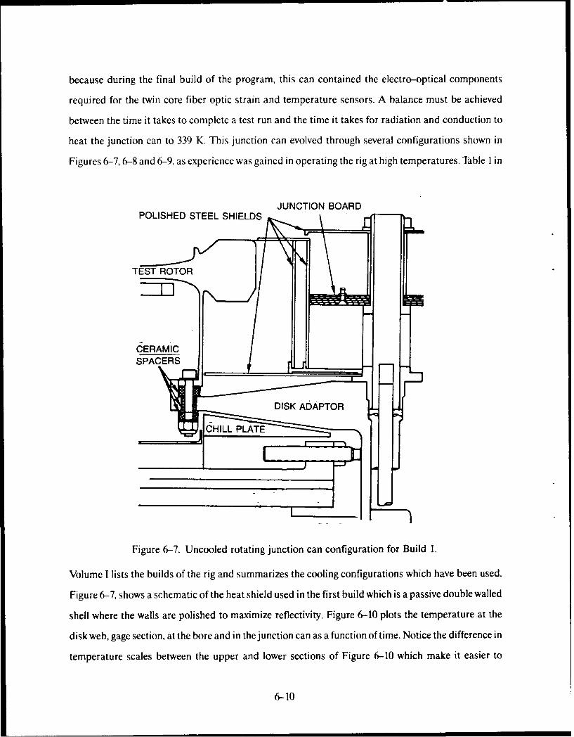
because during the final build of the program, this can contained the electro-optical components

required for the twin core fiber optic strain and temperature sensors. A balance must be achieved

between the time it takes to complete a test run and the time it takes for radiation and conduction to

heat the junction can to 339 K. This junction can evolved through several configurations shown in

Figures 6-7, 6-8 and 6-9, as experience was gained in operating the rig at high temperatures. Table I in

JUNCTION BOARDPOLISHED STEEL SHIELDS

TEST ROTOR

SPACERS .

DISK ADAPTOR

CHILL PLAT E

Figure 6-7. Uncooled rotating junction can configuration for Build 1.

Volume I lists the builds of the rig and summarizes the cooling configurations which have been used.

Figure 6-7, shows a schematic of the heat shield used in the first build which is a passive double walled

shell where the walls are polished to maximize reflectivity. Figure 6-10 plots the temperature at the

disk web, gage section, at the bore and in the junction can as a function of time. Notice the difference in

temperature scales between the upper and lower sections of Figure 6-10 which make it easier to

6-10

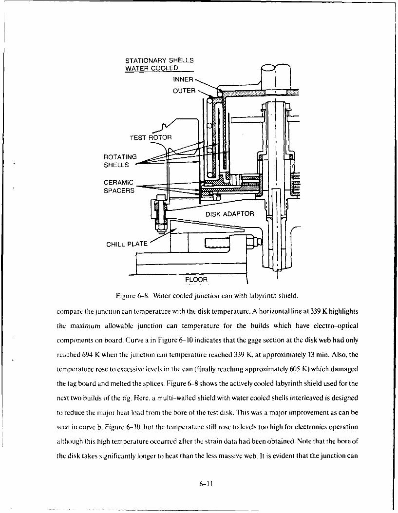
STATIONARY SHELLSWATER COOLED

INNER ]

OUTER r :::

TEST ROTORROTATING

SHELLS - g

CERAMIC %%- A 1SPACERS ------

DISK AtDAPTOR

FLOOR

Figure 6-8. Water cooled junction can with labyrinth shield.

compare the junction can temperature with the disk temperature. A horizontal line at 339 K highlights

the maximum allowable junction can temperature for the builds which have electro-optical

components on board. Curve a in Figure 6-10 indicates that the gage section at the disk web had only

reached 694 K when the junction can temperature reached 339 K. at approximately 13 min. Also, the

temperature rose to excessive levels in the can (finally reaching approximately 605 K) which damaged

the tag board and melted the splices. Figure 6-8 shows the actively cooled labyrinth shield used for the

next two builds of the rig. Here, a multi-walled shield with water cooled shells interleaved is designed

to reduce the major heat load from the bore of the test disk. This was a major improvement as can be

seen in curve b. Figure 6-10, but the temperature still rose to levels too high for electronics operation

although this high temperature occurred after the strain data had been obtained. Note that the bore of

the disk takes significantly longer to heat than the less massive web. It is evident that the junction can

6-11

BALANCE RN

STATIONARY WATERCOOLED COPPER SHELL ELECTRO-OPTIC

ROTATING SHELLS

TEST ROTOR

SPACERS .

DISKADAPTORSHIELD DISK ADAPTOR

FLOOR

Figure 6-9. Final configuration of junction can.

temperature heating rate tends to follow the bore temperature because of its close proximity rather

than the web temperature. Evaluation of the temperature data on the adaptor disk and inside thejunction can indicates that an important heat path is radiation from the hot disk to the rim of theadaptor and then by conduction toward the center and then up the center tube. To increase the thermalresistance of this path and reduce the heat load into the junction can, an additional stationary shield

has been added as shown in Figure 6-9.

Build 3 incorporated this shield but was terminated before any high temperatures wereattempted. Build 4 incorporated a "hybrid" shield in that the main shield was the passive double wallreflector, but it also included the adaptor shield. The temperature response of this configuration isshown in curve c of Figure 6- 10. This shows that even without the water cooled labyrinth the response

6-12

i200- DISKBORE

1100-

1000- DISK TEMPERATURES

900-wa:D 800-

< 700-W DISKn 600-W~WEBWF- 500-

0- 400-

300-

200-

100-

~- 400JUNCTION CAN TEMPERATURE

300- (a) UNCOOLED

0 (c) UNCOOLED WITH5 / / AD-APTOR S H IELDz 200- /DESIRED ,.

.- /-UPPER LIMIT I"Qo10- ... ... - --c-o-W

0 10 20 30 ,0 50 60 70 80 90 100110120130140

-DATA ACQUISITION COMPLETE

TIME (min)

Figure 6-10. Comparison of disk and junction temperatures.

rate was much slower than curve a. Additionally, a scheme to promote rapid cool down and prevent

high junction can temperatures after the test was implemented by the test stand per.-onnel. Provisions

were made in both the water cooled shield and the adaptor shield for a flow of cooling air to be

introduced from one of the lid access ports. This is accomplished after the test data acquisition is

complete by slowing the rotor to around WO1 r/min, shutting off the heater, releasing the vacuum,

removing the inspection port, and introducing shop air to the pipe just inside the lid. This provides

forced cooling to the sensitive electronics and the adaptor rim and reduces the temperature increase

which was occurring after data acquisition was complete.

6-13

It is judged that with post-test cooling, the configuration shown in Figure 6-8 would be

satisfactory from temperature considerations, but another factor suggested that a further

modification would be beneficial. This centers around the fact that the ceramic insulating spacers

used for configuration in Figure 6-8, were not able to survive the rotational loads. Upon teardown after

Build 2, the ceramic spacers all exhibited fractures or severe cracking. Although the fragments of the

failed spacers were all contained by the metal shells, the fact that failure was occurring introduced the

possibility of the junction can shifting at high speed which could create a potentially hazardous

imbalance condition. During an early build phase, the junction can (now containing the electro-optical

components) did shift due to imbalance of the components. This shift increased the contact load on

the ceramic standoff at the base of the stack to the point where it failed, increasing the imbalance to the

point where rubbing occurred between the rotating and stationary elements of the shield, and the

instrumentation connections failed. Thus the reason for redesign is to provide a stronger, stiffer

metallic support for the instrumentation and to provide for component balance of the package before

assembling with the disk system. An attempt to regain thermal resistance of the parts comprising the

can (lost by elimination of the ceramics) has also been implemented by reducing contact area to a

minimum, and flame spraying 0.38 mm Aluminum Oxide at contact surfaces. The water cooled shield

around the can has also been simplified for better control on radial running clearance. It was

anticipated that during the final build with the simplified water cooled shield and the reflective skirt

around the adaptor disk that the temperature in the electronics can would have remained below the

specified 339 K.

5. TEST HARDWARE

The test rotor on which all of the sensors were mounted is a high pressure turbine rotor from an

aircraft jet engine. In order to simulate as closely as possible the actual inertial environment of the

engine, the disk was fitted with a full compliment of blades as well as side plates and seal rings. Figure

6-11 shows a meridional view of the disk and related assembly components with some relevant

dimensions.

Stress and thermal analysis performed on a model of the disk is described in Section VII.

6-14

89 mm 130.6 mm 233 mm 300.8 mm226 mm

RADIUS, mm

Figure 6-11. Cross-sectional view of a test rotor.

6. DATA ACQUISITION SYSTEM

A schematic of the data acquisition system is shown in Figure 6-12. Strain gage excitation and

conditioning is supplied by UTRC designed and built signal conditioning units. Adjustable regulated

bridge excitation voltage, polarity, shunt calibration, and balance are provided. The test strain gage

comprises one arm of the strain gage bridge and is connected in the conventional three wire

configuration. The bridge completion resistors are stationary and are located adjacent to the slip rings.

While it is not good practice to have the active arm of a strain gage bridge in a switched or slip ring

circuit, bridge stability required locating the bridge completion resistors away from the high

temperature around the disk.

For accurate temperature measurements, the extension wire from the thermocouple to the slip

ring rotor and from the slip ring stator to the data system uniform temperature block is the same

material as the thermocouple itself. To account for any temperature gradient across the slip ring

(where copper and silver alloys are introduced into the thermocouple circuit), an electronic

temperature measurement was made on the shaft at the point where the wires connected to the slip

6-15

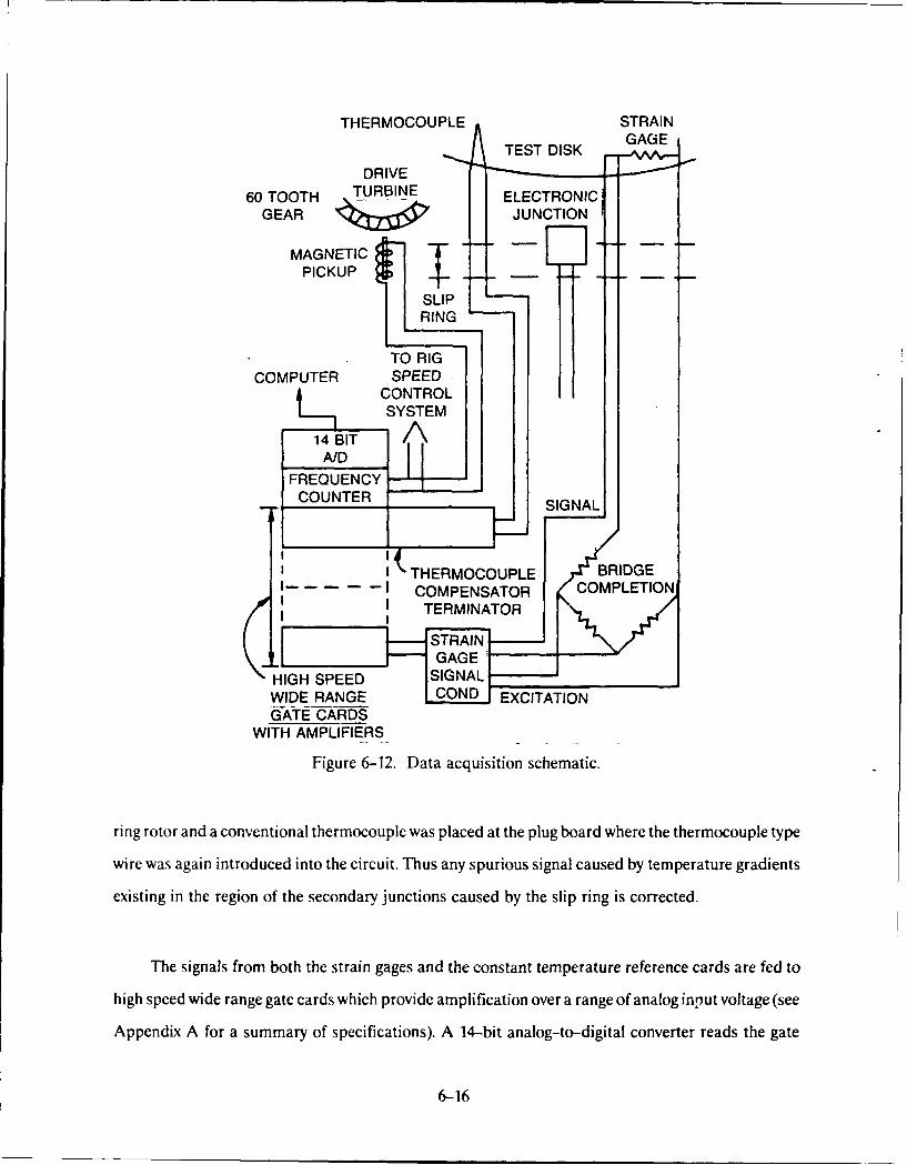
THERMOCOUPLE STRAINTEST DISK -

DRIVE -- "60 TOOTH TURBINE ELECTRONIC

GEAR JNTO

RING

RIGMENAO

COMPUTER SPEED

COUNP E R SSIGNAL

ITHERMOCOUPLE BRIDGE

W D RAI COM PN ATOR COM PLETION

GATE CARDSWITH AMPLIFIERS

Figure 6-12. Data acquisition schematic.

ring rotor and a conventional thermocouple was placed at the plug board where the thermocouple type

wire was again introduced into the circuit. Thus any spurious signal caused by temperature gradients

existing in the region of the secondary junctions caused by the slip ring is corrected.

The signals from both the strain gages and the constant temperature reference cards are fed to

high speed wide range gate cards which provide amplification over a range of analog input voltage (see

Appendix A for a summary of specifications). A 14-bit analog-to-digital converter reads the gate

6-16

outputs, digitizes, and transfers it to the Perkin Elmer computer for storage and manipulation. A

frequency counter card is paralleled off the magnetic speed pickup and the output stored.

Data are obtained by sampling each strain and temperature 200 times over a 1-second time base.

-On Line" computation is performed by calculating temperature based on a ninth order polynomial.

The strain calculation is based on the use of the standard single active arm bridge equations.

Figure 6-13 is a schematic of the strain gage bridge showing the three wire connection used to

minimize the effect of leadwire resistance.

/~ SHUNT

i.,t CALIBRATION

/

n

BRIDGE

A-ACTIVE STRAINGAGE

SIGNAL OUT

Figure 6-13. Strain gage bridge arrangement.

Resistance A is the strain gage, mounted on the disk and B, C, and D are the bridge completion

resistors mounted in the junction box adjacent to the slip ring. Resistors n and mn are physically located

in the signal conditioner and are used to achieve initial bridge balance. Throughout this program, the

strain gage bridges were initially balanced at the beginning of each build but no further adjustment of

the balance control was made. Residual imbalance was recorded, however, at the beginning of each

run.

6-17

The overall approach is to precisely measure the input values of resistance, calculate the bridge

constants, and use the standard unbalanced bridge equations to calculate the strain. Figure 6-14

shows pictorially the flow of data acquisition.

The equations are set up in a form to record the voltage at a data point and subtract from that the

voltage taken at zero speed.

This gives an overall picture of conditions on the disk. Additional information that is presented

in almost real time includes the airect mV reading, and a calculation of the standard deviation of the

200 points in digital counts. Standard deviation is of value in determining overall quality (steady state)

of the signal, which by its magnitude reveals such features as open circuit, induction heater "on" (the

heaer is turned off during actual data acquisition to minimize radiated noise) and slip ring noise. The

pararmeters are all written to tape for later reduction "off line" to correct the strain for apparent strain

due to temperature. and gage factor shift due to temperature.

The strain data, which are recorded during the test and converted on line to engineering units, are

based on room temperature values for gage factor, and no correction is made for apparent strain due

to temperature. An "off line" program is available which applies corrections for gage factor variation,

and apparent strain due to temperature, and for the "Chinese" strain gages, the apparent strain due to

rate of change of temperature.

Calibration of the gage factor variation with temperature is achieved by applying the reference

strain gage to a calibrated bar whose strain vs. deflection has been calibrated at room temperature.

The test bar is triangular in plan form to minimize the sensitivity of strain to exact position of the gage.

The bar with test gage mounted is heated uniformly, and a precise deflection imposed on the free end.

The strain output is then a function of geometry only and changes :n output are related to changes in

gage factor which is stored in the off line reduction program as a set of polynomial coefficients.

During fabrication and installation of the strain gages on the disk, gages were also installed on

simple coupons fabricated from the same alloy as the disk in order to calibrate the gage/disk

combination for apparent strain due to temperature. The coupons which had no mechanical load

6-18

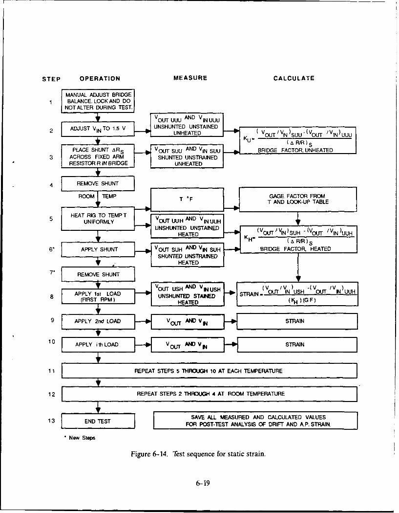
STEP OPERATION MEASURE CALCULATE

MANUAL ADJUST BRIDGE1 BALANCE. LOCK AND DO

NOT ALTER DURING TEST.

-i +i VOI UUU AND V IN UUUADJUST VIN TO 1.5 V UNSHUNTED UNSTAINED

UNHEATED ( V / N )SUU "(VouT VIN)UUU

S KU (A R/R)SPLACE SHUNT AR S - OUTS AND VIN SUU BRIDGE FACTOR, UNHEATED

3 ACROSS FIXED ARM SHUNTED UNSTRAINEDRESISTOR R IN BRIDGE UNHEATED

REMOVE SHUNT

ROM EM TO GAG3E FACTOR FROMT AND LOOK-UP TABLE

5 HEAT RIG TO TEMP T VOTUH AND V

UNIFORMLY INUUHUNSHUNTED UNSTAINEDHEATED K (V ou T ' N)SUH - (VouT /VIN )UUH

6__APPYSHUN___ANKHV (A RIR) S

APPLY SHUNT VMOUT SUH AND VI SUH BRIDGE FACTOR. HEATEDSHUNTED UNSTRAJNED

HEATED

7" REMOVE SHUNT

APPLY ist LOADVH YOUT USH AND V IN USH (V /V S (V /V

APPLY 1s LOAD UNSHUNTED STAINED STRA(FIRST RPM) HEATED (VH ) (G F)

9 APPLY 2nd1()llIl LOADI

10 APPLY ithLOAD-- VO AND V IN STRAIN

11 REPEAT STEPS 5 THROUGH 10 AT EACH TEMPERATURE

12 REPEAT STEPS 2 THROUGH 4 AT ROOM TEMPERATURE

13 EN TESTSAVE ALL MEASURED AND CALCULATED VALUES

13 END TEST FOR POST-TEST ANALYSIS OF DRIFT AND A.P. STRAIN.

New Steps

Figure 6-14. Test sequence for static strain.

6-19

imposed on them were then oven heated, and the strain gage output measured at various temperatures

during the excursion to maximum. During the heating of the specimen, care is taken to insure that it is

at a uniform temperature. The apparent strain output of the strain gage at various temperatures is due

to two effects: the change in specific resistivity of the gage alloy due to temperature, and the difference

in thermal coefficient of expansion between the gage alloy and the component on which the gage is

mounted. The values of apparent strain due to temperature are entered into the off line reduction

program as coefficients to a polynomial fit of the data. The order of the polynomial varied from four for

the Build 1 wire gages to nine for the "Chinese" alloy gages and the thin film gages.

In the case of the "Chinese" strain gages, the effect on apparent strain due to temperature was

extended to include the apparent strain due to rate of change of temperature. These alloys exhibit a

rate dependence, a correction for which was included in the program. The data for this correction were

obtained by heating the coupons as before to obtain the apparent strain, and then cooling them at four

different rates. Time, temperature, and apparent strain are recorded. At several temperature levels,

the rate of cooling is calculated and the delta R/R noted. The delta R/R is then cross plotted for each

rate at several temperatures. This information is stored on the off line reduction program as a ninth

order polynomial fit. In use in the off line reduction program, data points two before and two after the

point being corrected are used to establish the rate of change of temperature. The slopes during the

actual test are compared with the slopes during calibration and the "best" match is operator chosen. It

should be noted that during the test, data are acquired at uniform time intervals which simplifies slope

calculations.

The thermocouple used to supply the temperature information for strain correction is usually the

sensor that was attached to the disk in close proximity to each gage, but if that T/C was inoperative or

its reading was in error, another sensor can be chosen to use for the correction.

In addition to recording data from the sensors under tests, temperatures are recorded from a

number of critical locations on the rig. On the rotating assembly, in addition to the junction can

already discussed, temperatures are measured at the bore and rim of the test disk and at two places on

6-20

the disk adaptor. Stationary temperature measurements are made on the spindle bearings, on the heat

shield face of the lead bricks, and at locations on the floor and ceiling of the heat shield.

7. TEST PROCEDURE

In view of the rupI mass, temperature el;vironment. and speed, a word on balancing the rotor is

in order. Experience with the UTRC spin rig with a variety of test rotors has shown that even with

preliminary outside balancing of the test piece, field balance in the rig has always been required, so for

the ASI program the external balance step has been eliminated. The blades and side plates are

individually weighed and located around the disk to minimize residual imbaLnce. The turbine rotor

when mounted in the spin rig has a calculated first mode critical speed of 1350 r/rnin. The second mode

is around 29.00) r/min and is not a consideration for these tests. The rig ha, i classical lightly damped

resonant response and balancing is carried out at 8WM) to 1N) r/min. The mass distribution is such that

a singzle plane balancing technique is adequate, with the object of limiting the maximum resonant

amplitude at the plane of the vibration pickups to 6 mils or less (which is approximately half the level at

the plane of the rotor). Once above resonance, the amplitude is generally on the order of 1 mil up to the

maximum test speed of 13,200 r/rin. The actual field balance employs the three trial weight method

(see Reference), requiring four runs, one with no tria; weight and the other three with the weight at

various positions on the disk. The amplitude of vibration at a fixed speed is noted for each of the weight

locations and plotted vectorially relative to the amplitude with no weight. The intersection of the

vectors gives amplitude information proportional to the size of the weight required for balance, and

the angular orientation gives the location on the disk. This method has proven satisfactory throughout

the program.

To obtain data at high temperature, the rotor is brought up to an idle below critical speed and the

induction heater energized. When the desired temperature is reached, the rig is accelerated to each of

four test speeds up to a maximum of 13,200 r/min. When the speed is stabilized, the heater is turned off,

the shutter opened (for photogrammetry, and pyrometer rccords) and strain and temperature data

recorded. During the time it takes to achieve the next speed, the shutte, is closed and the heater

6-21

re-energized. This procedure requires approximately 30 min to acquire data points for both increasing

speed and decreasing speed after the desired temperature is reached.

8. CONCLUDING REMARKS

The UTRC spin rig now has the capability to acquire data at temperatures up to 950 K, at speeds

up to 13,200 r/min. The requirements for heat shielding and test technique have undergone substantial

changes over those originally planned, and now specified test conditions can be consistently achieved.

The test goals of the program have been met, and it is anticipated that future efforts will make use of all

the techniques developed during the builds described above.

9. REFERENCE

"Balancing a Rotating Disc, Simple Graphical Construction," I. J. Somerville, Engineering, 1954.

6-22

AlI''IKNIIX AD)ATA At QI ISiliO N SYSiIV 'ME NL PI ll Ai N

,A I

APPENDIX ADATA ACQUISITION SYSTEM COMPONENT SPECIFICATIONS

HIGH SPEED WIDE RANGE GATE CARDS (6 CARDS)

Number of Input Channels 8 per Card

Input Differential with Guard Shield

Isolation Transformer

Sampling Rate 100 Samples/Sec/Channel

Gain Accuracy +/- 0.025% of Full Scale

Linearitv +/- 0.025" of Full Scale

Full Scale Analog Input V 0 to 10.24 V in II Ranges

Input Impedance > 5 Mn

THERMOCOUPLE COMPENSATOR (4 CARDS)

Number of Channels 8 per Card

Inputs per Channel 3. High, Low, Shield

Reference Temp. Setting 0°C

Compensation Thermocouple

Error 0.025°C/°C Amb. Change

14-BIT A/D CONVERTER (1 CARD)

Gain Stability +/- 35 p/m per 3C

Gain Accuracy +/- 0.025% Full Scale

Linearity + /-0.025% Full Scale

Quantizing Error +/- 1/2 LSB

System Noise Maximum < I mVPP RTI + 1/2 LSB

6A-2

ViI. DiSK STRESS ANALYSIS

The disk that was used in the program reported herein is normally part of a high pressure turbine

assembly as shown in Figure 7-1. In this application, the gas loads on the rotor, and loads caused by the

seals and other appendages influence the strain distribution in the disk as well as the centrifugal

loading caused by the blades and the disk itself. In Figure 7-2, the spin rig configuration is significantly

difft'rcnt so that it was judged that analysis oftlie spin rig configuration would be useful in providing a

rcicrctce against which the measured strains could be compared A MARC finite element model with

rid breakup as shown in Figure 7-3, was used to evaluate the response of the disk to inertial loads as

well as some thermal gradients. Eight noded quad elements were used, and the model made use of

symmctr, about the rotational axis, and the center-plane of the disk. The resulting model contained

119,( clemcnts and 434 nodes. The region of the bolt hole circle at 203 mm radius, and the region of the

disk between the live rim and dead rim are assumed to carry no hoop load, which is modeled by using

,niso"tropic material properties for those elements with the circumferential modulus of elasticity set to

a very small (practically zero) value. The MARC analysis calculates disc self-loading due to rotational

speed, and the blade and side plate loads were input as discrete forces at the rim rather than including

them in the model. Since the area of the disk of interest, where the strain sensors are mounted is

located well away from the bolt hole circle and the point of load application where local effects might

be large. this approach was adopted. Boundary conditions were fixed by the axes of rotational and

disk-mid plane symmetry.

Comparison of bending and meridional strains for a high turbine first stage disk similar to the

one used in the ASI testing shows that the maximum bending strain generally comprises a small

(approximately 1(%) fraction of the total strain. The strain induced by the thermal gradients on the

other hand can be a significant fraction of the total. For the ASI tests, temperature was measured at the

bore and rim as well as at the gage section, but since there are no data in between, it was assumed for

the MARC analysis that the gradient is linear from bore to gage section, and constant from the gage

section to the rim (the rim thermocouples indicated only very small gradients in this region). Figure 7-4

shows the gradients assumed for the various gage section temperatures, and Figures 7-5a and 7-5b

show the resulting changes in gage section radial and circumferential strains. Note that only the strain

7-1

due to thermal gradient and centrifugal effects are shown; the thermal expansion effects have been

subtracted out. Since the actual thermal gradients in the disk are not known, the analytical strains

which are shown in Figures 1 and 2 in Volume I, are shown as a shaded region to indicate that the

calculated strain lies within it. In Figure 7-5 the cooler bore tends to increase the radial strains and

decrease the circumferential strain.

1ST STG DISK

. 2ND STG DISK

Figure 7-1. HPT module.

7-2

89 MM 233 mm 300.8 mm226 mm

RADIUS mm

Figure 7-2. Cross sectional of test rotor.

EXTERNI.LA -PaEO LOIAn BLA-f .SIDE PLATI

SOLT CICL AM .23

-- -- B CAC.ENTS

Figure 7-3. Finite element model of spin test disk.

7-3

10000 297 K ROOM TEMP# 422 K WEB0 589 K WEB

- 950 K WEB

800-

LU

I< 600-a:

400-

200 1 1 1 1 150 100 150 200 250

RADIUS (mm)

Figure 7-4. Assumed disk temperature gradients.

3000 L j CONSTANT ROOM TEMP

0 2000k<

10001 1140 150 160 170

RADIUS (mm)

Figure 7-5a. Radial strain at gage locations vs. thermal gradient, 13,200 r/min.

7-4

2600o 422 K WES# 589 K WES

- 0 755 K WE:0 950 K WEB* CNSTNT OOMTEMP

2400-

2200-

0

Z 2000

1800-

1600

1400 1 f140 150 160 170

RADIUS (mm)

Figure 7-5b. CIRC strain at gage locations vs. thermal gradient, 13,200 r/min.

7-5 *U.S. GOVERNMENT I'RINTING OFFICE: 1990 74&-564515