U.S. DEPARTMENT OF COMMERCENational Technical Infmonatin Seice

AD-A027 458

AN AIR POLLUTION ASSESSMENT OF HYDROGEN FLUORIDE

AIR FORCE ENVIRONMENTAL TECHNICAL APPLICATIONS

CENTER

MARCH 1976

- •

KEEP UP TO DATEBetween the time you ordered this report- search activities. And you'll get this impor-

which is only one of the hundreds of thou- tant information within two weeks of the timesands in the NTIS information coilection avail- it's released by originating agencies.able to you-and the time you are readingthis message, several new reports relevant to WGA newsletters are computer producedyour interests probably have entered the co0- and electronically photocomposed to slashlection. the time gap between the release of a report

and its availability. You can learn aboutSubscribe to the WeelWy Government technical innovations immediately-and use

Abstracts series that will bring you sum- them in the most meaningful and productivemarnes of new reports as soon as they are ways possible for your organization. Pleasereceived by NTIS from the originators of the request NTIS-PR-205/PCW for more infor-research. The WGA's are an NTIS weekly mation.newsletter service covering the most recentresearch findings in 25 areas of industrial, The weekly newsletter series will keep youtechnological, and sociological interest- current. But learn what you have missed Ininvaluable information for executives and the past by ordering a computer NTISarchprofessionals who must keep up to date. of all the research reports in your area of

interest, dating as far back as 1964, if youThe executive and professional informa- wish. Please request NTIS-PR-186/PCN for

tion service provided by NTIS in the Weekly more information.Govement Abstracts newsletters will give WRITE: Managing Editoryou thorough and comprehensive coverage 5285 Port Royal Roadof government-conducted or sponsored re- Springfield, VA 22161

Keep Up To Date With SRIMSRIM (Se!ected Research in Microfiche) microfiched report. Your SRIM service beginsprovides you with regular, automatic distri- as soon as your order is received and proc-bution of the complete texts of N.TIS research essed and you will receive biweekly ship-reports only in the subject areas you select. ments thereafter. If you wish, your serviceSRIM covers almost all Government ro- will be backdated to furnish you microfichesearch reports by subject area and/or the of reports issued earlier.originating Federal or local governmentagency. You may subscribe by any category Because of contractual arrangements withor subcategory of our WGA (Weefly Govern- several Special Technology Groups, not allment Abstracts) or Government Reports NTIS reports are distributed in the SRIMAnnouncements and Index categories, or to program. You will receive a notice in yourthe reports issued by a particular agency microfiche shipments identifying me excep-stuch as the Department of Defense, Federal tionally priced reports not available throughEnergy Administration, or Environmental SRIM.Protection Agency. Other options that willgive you greater selectivity are available on A deposit account with NTIS is requiredrequest. before this service can be initiated. If you

have specific questions concerning this serv-The cost of SRIM service is only 45. ice, please call (703) 451-1558, or write NTIS,

domestic (60ý foreign) for each complete attention SRIM Product Manager. I:

This Information product distributed by

m5 U.S. DEPARTMENT OF COMMERCENational Technical Information Service5285 Port Royal RceadSpringfield, Virginia 22161

UNITED STATES AIR FORCEAIR WEATHER SERVICE (MAC)

USAF ENVIRONMENTALTECHNICAL APPLICATIONS CENTER

1111!1IIIIllilllli11111 -SCOTT AIR FORCE BASE, ILLINOIS 62223

REPORT 7785

7' 71AN AIR POLLUTION ASSESSMENT

OF HYDROGEN FViJORIDE

By D DC

Capt Richard W. Fisher JUL 28 in l

D

March 1976

Approved for public release; distribution unlimited.

NAZOA IVWfr4FOVtMAfO URV1M

U~ 744n4

SReview and Approval Statement

This report approved for public release. There is noobjection to unlimited distribution of the report tothe public at large, or by DDC to the National TechnicalInformation Service (NTIS).

This technical report has been reviewed and is approvedfor publication.

J411 W. LOUERc-Chief, Editorial Section

FOR THE COIDI.LANDER

WILLIA1 E. BUCHAN, Major, USAFChief, Operations Branch

F--

.5o

ii

i~- -5

UnclassifiedSECURITY CLASS ICATIOW o F i1S PAGE (*Wsm " Dat_ __

REPORT DOCUMENTATION PAGE * RCA LET1G FOIM

.. GOVT ACCESSICN NO: FS.RCIE.TS CATALOG .UMOUR

USAFETAC 77854. TITLE (" Sew.:., e) TYPE OF REPORT & PERIOD COvERE

An Air Pollution Assessment of HydrogenFluoride

4-. PERFO .ING ORG. REPORT NUMMER

-. AUTHOR(.) 41- CONTRACT OR GRANT sUaUEmia)

Richard W. Fisher, Capt, USAF

S. PERFORMING ORGANIZATION NAME AND ADDRESS 10. PROGRAM ELEMENT. PROJECT. TASK

US Air Force Environmental Technical AREA 6 WORK UNIT NUMBERS

Applications Center (USAFETAC)Scott AFB IL 62225II. CON4TROLLING OFFICE NAME AND ADDRESS 12. REPORT DATE

US Air Force Environmental Technical March 1976Applications Center (USAFETAC) IS. NUUER OF PAGES

Scott AFB IL 62225 3014,, MONIITORING AGENCY NAME & ADORESS(UI 01frft ft.. Controlslng Office) IS. SECURITY CLASS. (of tlhe toPo) IUnclassified

IS. OECkASS1 iFICATION/DOWN GRADINGSCM LDULE

16. DISTRIOUTION STATEMENT (af ofte Report) -

Approved for public release; distribution unlimited.

I1. OISTRIUIITION STATEMENT (of the abstract entered in 81*0 20 it dffernt how Repo)

* Il. SUPPLEMENTARY NOTES

III. KEY WORDS (Contim au. reatvMerse aif necesarmy aut Identify by Nock aim bo)

Air Pollution Gaseous Diffusion

Dispersion Models Mesoscale DiffusionHydrogen Fluroide

2.AUSTRACT (Coathwe. on reveres side If necessary o"E fdonlityfir Nock umber).O~nly generalized conclusions aý)ut ground level concentrations (X)of hydrogen fluoride (HP) are possible when the place and time ofaerial release are unknown. HF is assumed to be a gas whenreleased from altitudes of 3 km ant'. 10 km and remains a gas during

the entire diffusion process. Three line-source models are solvedfor X/Q since the emission rate, Q, is unknown. H. Cramer'sconcentration model is the product of five terms, including an

DO JAN72; 1473 ,.oNO I, Nov61 IS oo r ii ,Unclassified _

SECURITY CLASSIFICATION4 OF THIS PACE (When Vale Entered)

Unclassified59CUONTY CLASSIFICATION OF THIS A9WeDo&WOM

edge effec s r oroe from Turner. Ground level dosages are

also-included. B. Turner's line-source model is a direct modif-ication of Sutton's basic diffu2sion equations and uses vertical

and horizontal standard wind deviations as calculated by Cramer.

The third model -8 an empirical derivation from Air Force testing

at the Cedar Hill Tower, Dallas, Texas. Results from these three

models graphically depict the maximum ground concentrations of HF

at 60 km downwind. Theoretically, when HF is released at 10 km

altitude the maximum ground concentration occurs beyond 100 km,

at which distance these equations become ineffectual.' However,

these estimated concentrations represent..only the worst meteoro-

logical conditions. Therefore, only when the mixing depth is

high will concentrated HF contamination occur. --.

iv Unclassified:SECURITY CLASSIFICATION Of THIS PAGEC(W1 DVale WIet.

PREFACE

The US Air Force Environmental Technical Applications

Center (USAFETAC) prepared this report in answer to areque3t from the Argonne National Laboratory, Argonne,

Illinois. The information is provided in support of theAir Force Weapons Laboratory (AFWL) Project 19008W15,

"Environmental Implications of Airborne Hydrogen Fluoride

(HF) Laser Operations."

Argonne National Laboratory requested USAFETAC supportin the belief that USAFETAC maintains a working computer

diffusion model for gases released from elevated line

sources. USAFETAC does not have a working computer model;

therefore, this report presents generalized conclusions

based upon a thorough search of references that present

information relevant to this problem.

In the event that this report is incorporated into

another report by the requester or any other agency,request that USAFETAC be furnished a copy of tae newreport in all cases where such dissemination is not

prohibited.

USAFETAC prepared this report for a specific purpose;

therefore, any further application of this information

should be undertaken with caution. Work on this reportprogressed under rigid constraints of resources including

time, personnel, equipment, and data. Department ofDefense agencies and their contractors should contactUSAFETAC directly for aid in assessing the applicabilityof this material for their purposes. Other prospective

users should contact prc'!essional eDvironmental analyts

in the National Oceanic and Atmospheric Administration

(NOAA) or private industry for simila~r assessment service.

v

....... X

_____-

TABLE OF CONTENTS

Page

Introduction . . .. . .............

Assumptions .. ... . .. .. ........ 2

Data Provided . . . . . . . . o . . . . . . . . . . 3

Summary .. . . . . . . . . . . . . . . . . . .. 3

Discussion ....... . ............. 5

REFERENCES a . . .e.... 17

APPENDIX ACalculations for Cramer's Generalized

Concentration Model ............ .. 18

ILLUSTRATIONS

3Figure 1. X/Q (Sec/m ) at Altitude of Release . . . 8

Figure 2. Estimated Ground Level Concentration/Emission Rate (x/Q) Versus DistanceDownwind When HF Gas is ReleasedFrom an Altitude of 3 Km . . . .... 9

Figure 3. Vertical Term of Cramer's ConcentrationEquation Versus Distance Downwind WhenHF Gas is Released from an Altitude of10 M 1... 0

Figure 4. Estimated Ground Level X/Q (Sec/mr)Versus Distance Downwind When HF Gasis Released From an Altitude of 10 Km . 11

Figure 5. Centerline Dosage Value (x/Q) at Altitudeof Release Versus Distance Downwind . . 12

Figure 6. Estimated Ground Level Dosage (x/Q)Veraus Downwind Distance When HF Gas isReleased From an Altitude of 3 Km . . . 13

Figure 7. Estimated Ground Level Dosage (x/Q)Versus Downwind Distance When HF Gasis Released From an Altitude of 10 Km . 14

vi

f ~)~--

Figure 8. Concent.. ation/Emission Rate, x/Q, andReleaz:.% Height Versus Downwind Distance-rom Cedar Hill Experiment ...... 15

Figure 9. Concentration/Emission Rate, x/Q, atGround Versus Distance Downwind FromTurner at Two Release Altitudes. . . . 16

Figoin A-5.. Relatioi.ship Between the Wind Speed2 Mete.s Above the Ground and the1- Minute Star lard Deviation of Wind,•7 ,:uth Angle (aA) in the Daytime• = ,.: . .. . . . . . . . . . 19

Figure A-2. -x.c:,.dard Deviation of VerticalConcentration Distribution (az)Versus Distance D(,nwind . ..... 27

F'igure A-* Vertical Term of Cramer'sConcentration Equation for aRelease Altitude of 3 Km ...... 28

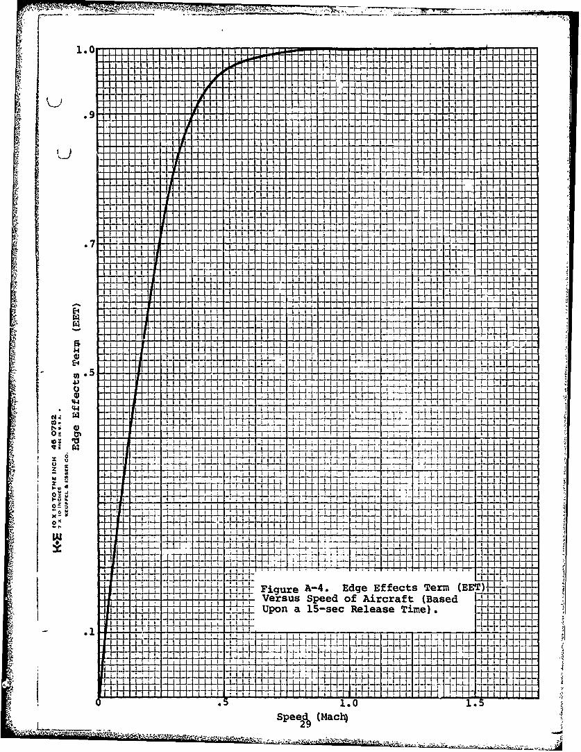
Figure A-4. Edge Effects Term (EET) VersusSpeed of Aircraft (Based Upona 15-Sec Release Time) . ...... 29

TABLES

Table I. Estimated Ground Level Concentrations . . 4

vii

Ilk

AN AIR POLLUTION ASSESSMENT OF HYDROGEN FLUORIDE

Introduction5.The purpose of this report is to estimate the

diffusion characteristics and downwind concentrationsof hydrogen fluoride (HF) after it is released from anairplane. The author conducted an exhaustive searzh ofUSAFETAC's in-house technical library to det~ermine amethod or methods adaptable to this problem.

Several authors have modified Sutton's basic diffu-sion equations for microscale analyses. Applicationsfrom three sources are included in this report. Themost useful model# H. H. Cramer (3), offers a generalized:oncentration model for a finely divided particulate orgas using the Gaussian distribution functions. Thesecond modell, applied by D. B. Turner (9), rewritesSutton's (1932) concentration equation into a simplified

S~finite line source model i.ncluding an edge effectsterm %'ET). This term is also applied as the EET toCramer's Generalzed Model in this report. The thir %

model is a reapplication of an equation by Smith and Hay(1961) using vertical turbulence intensity (7). The USAir Force empirically tested the diffusion characteristicsof airborne substances near Cedar Hill, Texas and thenappropriately modified the original equation. Understeady-state conditions, estimates can be made using these

equations for distances of up to 100 kilometers. Theseline-source equations are briefly described in this report.However, the classical diffusion equations are not appro-

pyi

Assumptions

The state of the art of diffusion estimation and thelimited amount of input data require that several assump-tions be made. They are:

"5 .3

(1) Diffusion in the alongwind or x-direction canbe neglected when compared with a strong transport wind

(5:13).

(2) In the vertical direction HF assumes a statis- $

tical Gaussian distribution.

(3) The emission is an instantaneous line source.

(4) Homogeneous steady-state conditions exist (i.e.,no space or time changes in wind or turbulence).

(5) HF reflects perfectly at the surface (i.e., no

ground absorption) and at the height of the mixing layer.

(6) HF remains a gas.

(7) No HF coalesces with water vapor, or washes

or rains out.

(8) HF has approximately the same molecular weightas air (i.e., no thermal buoyancy or settling velocity).

(9o Atmospheric stability is neutral at all pointsdownwind. ;

(10) Mixing height equals height of release.

2

I

4€

(11) The mean wind direction is normal to the air-

plane's flight path.

(12) No vertical wind shear at any point.

(13) The emission rate is constant.

Data Provided

We are given or can calculate several pieces of

information.

Mean Wind Speed (m) = 20 m/s (45 mph)

Sampling will take place near the surface therefore

z =2 meters

Four runs will be made:

Run Speed of Aircraft Altitude of Length of

Mach (m/s) Release (H) Release (y)

(1) .5 (230) 3 km (10,000') 3,450 m

(2) 1.5 (760) 3 km 10,350 m

(3) .5 10 km (33,000') 3,450 m

(4) 1.5 10 km 10,350 m

SummaryHydrogen fluoride (HF) is a very stable substance

in the atmosphere. Anhydrous HF or partially hydrolyzed

HF is completely soluable in the presence of sufficient

quantities of water vapor. Thus, in order to avoid

coalesence and precipitation scavaging, no water vapor is

3

assumed to be present. At various temperatare and

pressure conditions present in the atmosphere HP may

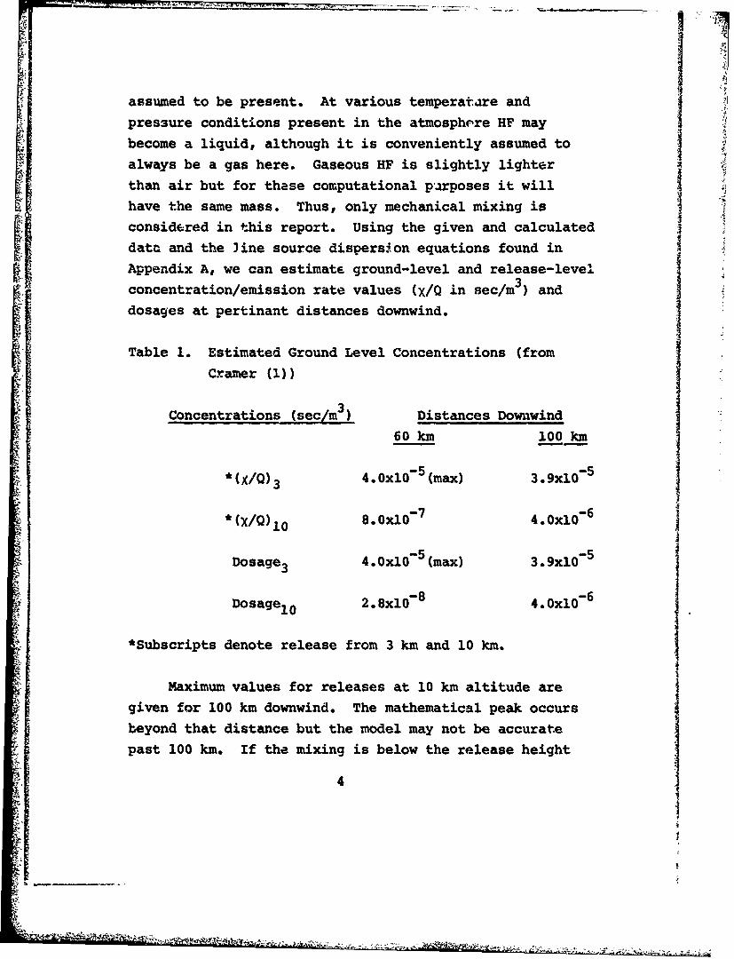
become a liquid, although it is conveniently assumed toalways be a gas here. Gaseous HF is slightly lighterthan air but for these computational parposes it willhave the same mass. Thus, only mechanical mixing isconsidered in this report. Using the given and calculateddata and the line source dispersion equations found inAppendix A, we can estimate ground-level and release-levelconcentration/emission rate values (X/Q in sec/m3 ) anddosages at pertinant distances downwind.

Table 1. Estimated Ground Level Concentrations (fromCramer (1))

Concentrations (sec/m3 ) Distances Downwind60 km 100 km

* (x/Q) 3 4.OxlO-5 (max) 3.9x10-5

*(X/Q)l0 8.0xl0 7 4.0xl0 6

Dosage 3 4.OxlO-5 (max) 3.9x10-5

Dosage1 0 2.8x10-8 4.OxlO-6

*Subscripts denote release from 3 km and 10 km.

Maximum values for releases at 10 km altitude aregiven for 100 km downwind. The mathematical peak occursbeyond that distance but the model may not be accurate

past 100 km. If the mixing is below the release height

4

of the HF gas, virtually no ground contamination willoccur.

Consistant and accurate meteorological inputs areparamount for the successful application of any pollution

concentration estimation method. Among the meteorologicalparameters, the miXing depths downwind from the release

point are the most important factors in determining cloud Iexpansion and ground contamination.

The assumptions made at the outset of this report Imake the expected concentrations extreme worst case figures.This conservatism means that under virtually all meteoro-logical conditions, the expected concentrations will notexceed those given.

DiscussionUsing Cramer's equation (3:21) we can calculate

center line concentrations and graph the results for

x/Q values at the release height (Figure 1) or at theground level when released from 3 km (Figure 2). When HFis released from 3 km, the maximum ground level concent-ration occurs 60 km downwind and the corresponding x/Q isis 3.22xi0-5 sec/m3n

When HF gas is released from an altitude of 10 km,the maximum concentration theoretically occurs 200 kmdownwind and is about 10 sec/m3. However, Cramer'ssteady-state equation is not valid beyond 100 km. At

this distance x/Q is about 5.2x0-6 sec/miThe EET (Figure A-4) is a function of the length

of the spray line, y, which, when considering a constantemission time, varies directly with aircraft speed. Thus,at Mach 0.5, the concentration values at either .dge ofthe 3450 meter spray line falls off by only 4% while atMach 1.5, virtually no concentration loss can be noticedat the spray line's edge.

5

n;

Figures 3 and 4 Sive the vertical term (VT) versusthe distance downwind for a release altitude of 10 km.Similar calculations for using the edge effer.ts term canbe made for the release height.

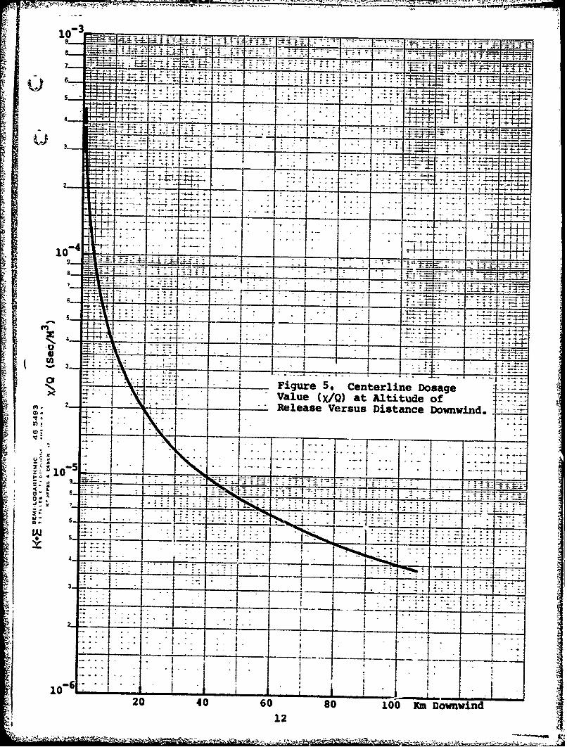
Figure 5 illustrates the estimated center line dosageterm versus distance downwind. This is interpreted as theamount of HF that passes a point during an entire sprayepisode. The EET (Figure A-4) is applicable to the dosageterms as well.

Figures 6 and 7 show the expected ground levelconcentration of HF when released from an altitude of 3 kmand 10 km respectively.

Other investigations to determine the actual downwindconcentration from elevated line sources have been con-ducted using empirical experiments. Among them was an •

Air Force test at the Cedar Hill, Texas television tower(7:171). The Air Force released traces of zinc cadmiumsulfide from a low flying aircraft while sampers were

placed at regular intervals downwind to 48 km. Theexperimenters related cloud expansion to meteorolo,aicalparameters including vertical and horizontal turbulenceand wind velocity. In a well developed turbulent layer,estimated ground level concentrations agreed well withthe mathematical model listed below.

C/Q = exp- 1)

"For releases above this turbulent layer, ground exposureswere much more erratic than predicted by the model (1:171)."

'When vertical turbulence is unity the released alti-tude concentration can be plotted for distances downwind(Figure 8). Cramer's VT, calculated above, can be usedtogether with the above C/Q to estimate ground levelconcentrations.

6

Turner (9:41) developed an equation to estimatedownwind concentrations at the ground from a finite linesource. The wind must be normal to the spray line. Thestandard deviation in the vertical, a , is taken from

the calculations for Cramer's model.Figure 9 is an illustration of the estimated down-

wind ground concentrations from Turner's equation:

X/Q- 2 [l/2(_l/2cH)2J (2)2w azu ezp

zaFor distances greater than 100 km downwind, in the meso-scale under turbulent conditions, or in the macroscale,the classical diffusion equations are not appropriate.Predictions of concentration distributions are moreaccurately made with synoptic forecasts of the movement

of large air masses. USAFETAC does not have the capabilityto make large scale turbulence predictions at this time.

7

,.I•

I-_ _ _

2•

--r-

T -7. - - -"'- 4 " -

4 ' 6 . , , . .. : -

-I"I ..

I0_- - -" "1* " :

L.u.':J-K'. L II I I"

-.- i 7•: -, -- 4I• • . •- - - -I - -

•:: : - - -.... t - ! i - , . . --

10-4

-"10.5 ..

4 I ,I I i

1 7'-- .-:.: -.- -.. i: -_ _ • _ _ , L'~i t 7-

-- + •.- :- " -" ' ; ""-" '* -

-Figure 1 x/ (Sec/m3 at

:"-: - ,

S ' titude of lea Ie.

10-6i,20 40 60 '' 80 100 IK' Io n a~n

I . -______

_________ T -. A.

~-17

II

i-4"-. ' -" ------ ' • - --'.. . -.-. *4.-*4 . . .t4 -

... 6. .. . . - .

II -4 ~+4.4

1 0- " '1- T""-"

:L i jo ýT- : r

V- U 4. 4t

.- , :. LI•r '-4nrtonEiso Rt XQ -- :2

01 . . ..".

1-4 ---1

x4 4!ý 7,; .

.41.1Ar11" ' 0 : ?.-:, .-+ -.. .. .. , .• I

TI of t

1: . . .4 . . . ...-

mU* ii-. d4 -- - 1.. .. '"4t¢ .• • ', .- ' . : = -.-, , - 4--.

7t T] -

U . ~~~~~t~zft:1t4- -4 -_ - -" - 4-f - 1- 1 f

t T +I

3 ---T74.

101

4ý4

3D _ _ J

*T V

10 _ -TH -J7

4-r.

S* ,. Figure 3. Vertical Term ofCramer'sa Concentration Equation

- IJ Versus Distance Downwind When HFGa iLs± Released from an Alitd

4--.-. r. ~

20ji :i>9 40 60 -0 9 0 K Downwind

10y

Mj II 1x

- - - -

_iu4 Estimaed Grondov3 _

10-0

20 406 olo mDwwn

-i-iEx-

41-r

4ý

* -*-

--410i

IN *

_I Vau XI t liueo

10 -5 -._ __I ~ -..1 7

Fiur 40 CenterlineK Dosagewind*

17112

* *.. . .- :- , .

S.. . . .. . ! _ , .. . .i -T .2 - . " . .

7-• i.i---; . "---------------,- l------

-: ! -i - _ --- _ -3 -

-T ..10I "I.LJ , I, i .-. 1

, . j-0 ,._ 4 .__ _ _ _

I 1 vi

__,I -4 -

3-. -i I 4• !,_ _ _ _. 2 . . . .

K ** , *I*] "*1******" ! T ,. . iue6 si__ated Grun_ ve

, l- ii' i I" ! Distance when HF Gas is Releasedii :| i -] . '1 .... from an Altitude of 3 km. . ..

.. ,-4 - t- -,-- . . t. . r..-....1.. .. " . . .

10 -10

!2 ;II I t

I - L _ _ ..__ I __--__ __ . ... ..___ __ _ ...... .

131

2 I j

20 400. 010

. 4 2i

7-.~-~~ - 7-- -r - ---- m

I t

- -- -

Fiur -7.- ' Esimae Grudee

10.2_0 40 60800 K owwn

14 _ _ _

-i.-. - S _ ___AC

4... _ . .

-4 I J IIII 1_ 1 1 • . , ,•

1 -64 N. .. .

ttI

" !-.1, : , ::I . _ _ . _ __ '4'

Height versus ! D a20 -4- I6 8 4i wi.

-67 7% I _ • : I ]- _ I

-, :. - I

-4 • .t t i I.

- t * . .' i

•: ! -~ . *. .. .

-, ~ I

.---- ....... ,..-- .... _fromCedar__illExperiment___,

"_ 1, I _ _ _ __,,-. -=- - -1----*-1---.---____

-1oe " ' _I I I I I I I I I II I I I I

151

-*. .. i-, ' "" i " '•'• +''•••... •••,I _.•->•• "; :,• '',,' '-

10-5

4---

i0-6 •

SR I

I

1 16

I I !,

t 0- i •.I'

i I______ I

___I______ I :

_-__ 1~ .isin•e /Q tG'~

.H ~ -7-_-versu Disanc Don ind oS:: : -- *......1

Turner- at Tw ees Attds

22 ..... .. . . _ ._______

20___ 40 60 8 r0 1 onwn

_________________________________ ___________________________

REFERENCES

(1) Air Pollution Meteorology * US Environmental Protec-tion Agency# Research Tri.angler North Carolina,August 1973.

(2) Burrington, R. S.: Hadokof Mathematical Tables

(3) Cramer,, H. E.,, et. al.: "Technical Report - Develop-ment of Dosage Models and Concepts," GCA TrechnicalReg rt No OR7-15-G, GCA Corporatio-n-,Co-nt-r-ac-tNo.DAD96--02TI e 1972, 367 pp.

(4) Dettling, R. E.: A Line Source Mod-al for Assessingthe Gravitational Settli-n-gDiffUSion Associated withAeilSryn prtos USAPETAC Report. 7496j7

(5) Munn., R. E.,, et. al.: Dispersion and ForecastingAir Pollution, Technical Note No.-T121, -World Meteor-ological organization, Geneva, Switzerland, 1972.

(6) Putta, S. N., and Cermak, J. E.: "Mass DispersionFrom an Instantaneous Line Source,," Technical ReportNo. 19, Office of Naval Research Contract No.N00014-68-A-0493-000l, Project No. NR 062-414/6-6-68Code 438, June 1971, 91 pp.

(7) Slade, D. H., Editor: Meteorology and Atomic EnergyEnergy 1968, US Atomic Energy Commission/DivisionOfThicaT Information, Oak Ridge, Tenneiiseej, July

1968.

(8) Sutton, 0. G.: Micrometoooy McGraw-Hill Book

(9) Turner, B. D.: Workbook of Atmospheric DiseersionEstimates, US Dept of Health, Education, and Welfare,Public Helth Service National Air Pollution Control

:1 _____Administration, Cincinnati, Ohio,, 1969. SA

I!

Appendix A

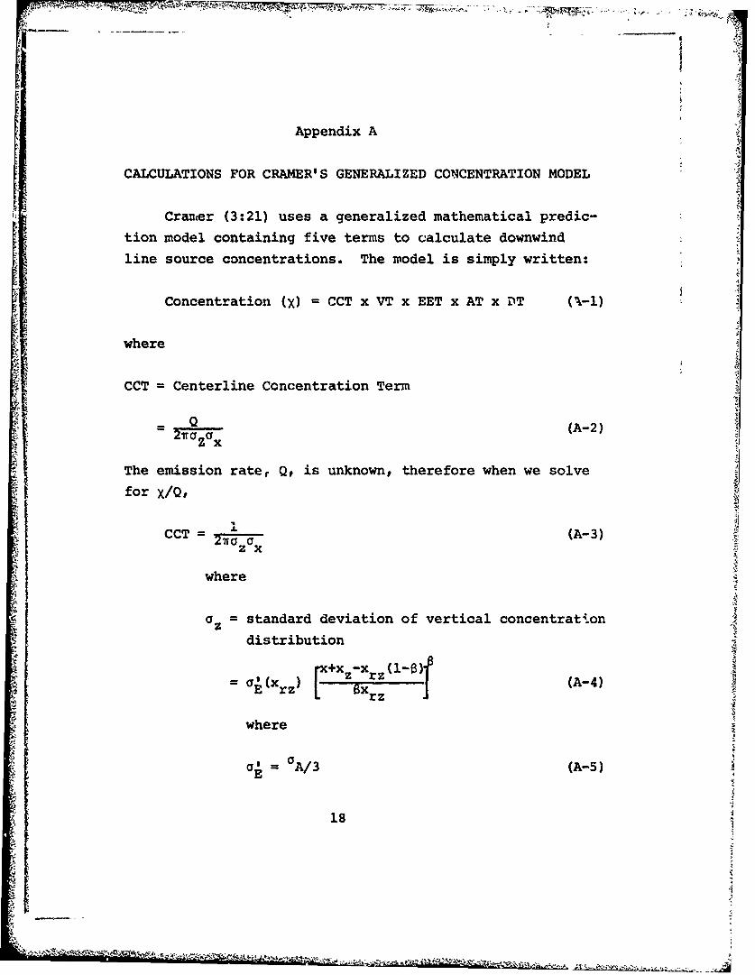
CALCULATIONS FOR CRAMER'S GENERALIZED CONCENTRATION MODEL

Cramer (3:21) uses a generalized mathematical predic-

tion model containing five terms to calculate downwind

line source concentrations. The model is simply written:

Concentration (X) = CCT x VT x EET x AT x DT (C-l)

where

CCT Centerline Concentration Term

Q- 2 zr x a(A-2)

The emission rater Q, is unknown, therefore when we solvefor x/Q,

• 1.

CCT =-z (A-3)z x

where

az = standard deviation of vertical concentratton

distribution

+Xz-x (= (Xr ) (x 8x (A-4)

where

a' = A/3 (A-5)

18

where

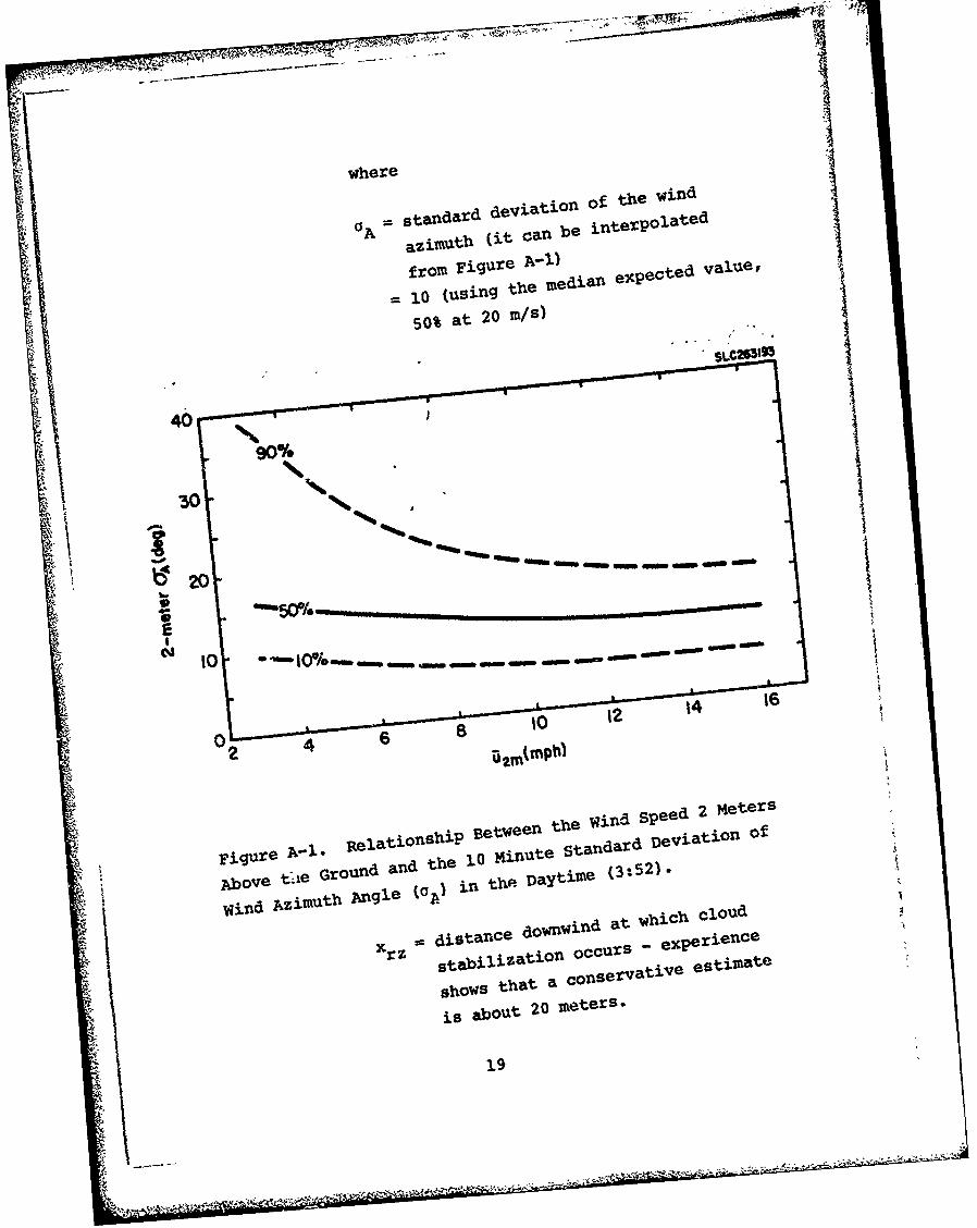
standard deviati-on of the wind

a~i~lU~(it can be interpolated

from V'igure A-1.) aa xetdvl

10 (using the med-a ,p~tdvle

50% at 20 m/s)

40

:0 "Wa -A - O W 0

I G0ommo

14 16

pigreA-..Relationship Between th id Dpeedaio 2Ofee

pigbv t ro n a dte 1.0 MIinu~te Sta nd ad D vi t on o

Azimu t ha (0?) ad h (3:52).

Wind ,t Angle pin the. DaYti2le

wind distance downwind at which cloud

x tblzto ocrs - excperience

shows that a coflse~,tv

si

is about 20 meters.

19

- vertical diffusion coefficient (3:63)references sources that show this valueapproaches unity for elevated releases

under neutral conditions.

x = vertical virtual distance - when thestandard deviation of the verticalconcentration distribution is amall,this value

= zR - X (A-6)

= 1/3.3 = 0.30

X = distance downwind at which the

standard deviation of the vertical

concentration distribution i%measured

-= (since we are interested onlyin the standard deviation at thesource)

thus, as an example, assume that we are interested in aS"istance 10 km (10 4 m) downwind,

then

104+0.3-20(1-1) 1az = .052(20) 1(20) (A-7)

500

Figure A-2 plots all az for distances downwind to 100 km.

20

al,

____ ____ ___ ____ _ ý

a standard deviation of the downwind concentration

distribution.

1 (using assumptions (1) and (12))thus,

CCT/Q 1 3.14xi 4 sec/m (A-8)

for a release altitude of 3 km at a distance of 10 kmdownwind.

VT = vertical term

[ imH-z 2H[ 2i++Zz 2

- exp e1/2 + exp 1/2(-

the z-ieto hr o u 1

2iHg-H-z 2 21H mH+z 2

oz = 0 at1 m

fir on ie ato

T (exp -1/2 + exp 1/2

+ exp [1/2 0 + exp-/2 (A-9)

The vertical term refers to the expansion of the gas in

the z-direction where for Run (1)

H =height of release 3000 m

z height of interest 2 m (ground level)

Hm3000 (see assumption (1))0 500 m (at 10 km)

for one iteration

VT exp 1/(500 ]+ exp 1/2( 500F

2I 2exp -1/2( 5000 2 + exp 1/2 00-30

21

ep 1/2(+ exp[~l,2 .O+39.22)J+_., ,2 6000+0002,Q2)2

= exp(-18) + exp(-18) + exp(-18) + exp(-18)

+ exp(-162) + exp(-162) (A-10)

VT - 4 exp(-18) + 2 exp(-162) (A-I1)

- 1.52x10-8

Only one iteration is used in the vertical term calculationbecause succeeding iterations become negligibly smallrelative to the total vertical term. Figure A-3 relates thevertical diffusion term with downwind distances.

•ET = P2 I exp (-1/2p2 )dp

en e(.i/2p +- 2 (Turner (9:41)) (A-12)27pi=2 I~n3S+ |E(2n-3)|

n=2 P1

where

"Pl = Y1 and P2 Y2•. ay a

Gy

when the spray line stretches from yl to Y2'

and

22

L-

-y[(a~~)ryXx -x (1-az) 1/U (yaT) xr vY ry uI+ (Ae'x)1 2

ax /y(A-13)

where

I I

where

T emission time - 15 seconds

'To reference time = 600 seconds

G('TO) =standard deviation of theangle measured over referencetime (TO)150 = .263 radians (from

Cramer (3:53))

GA(-t) 151/53 . 263(.025).2

=158x10-4

Xry =distance atwhich crosswind cloud

stabilization occurs downwind from

source -

40 meters (from Dettling (4:12))

x - 1 meters (fo xml nEquationA-7)j

XY-crosswind virtual distance

23

*MOW-----~

I Ry

where

YyR " standard deviation of the cross-wind distribution

XRy = distance at which the standard

deviation of crosswind concentra-tion is measured

=0

a= .*rosswind diffusion coefficient-1

AO = azimuth wind direction shear betweenground level and release level

= A- (z 2-zI) (A-16)

where

44AeE- = rate change of wind direction

from surface to release height

(radians/meters)

Since the HF is released well above the gradient level, theangle between the surface and gradient level is assumed tcbe 450 as estimated by Sutton (6:71).

.14 radians (A-17)"! W meters

24

-- -- ... .

- 0.47x10 4 radians/meters

z - effective upper bound of cloud- 3000 meters

z - effective lower bound of cloud

= 2 meters

Ae' = 0.47x10 4 (3000-2) (A-18)= .14

thus

= -4 10 +1-40(1-1) 1) 2+ (.14x10-1)•y= 1"8x°-141 ')40 } "4.3'

(A-19)

= 811 meters (for a distance 10 km downwind)

Finally, to calculate the limits of the EET summation term

yl, 2 - distance from centerline of cocicen-tration

= 1725 meters

then

P1,2 12 2.13 (A-20)

+2.131 1)2)dEET- J - exp (-1/2(2. (A-21)

-2.13

25

- .9668 (from Burrington (2:273)) for a samplingheight of 2 m when HF is released from a height

of 3km.

Figure A-4 expresses EET relative to airplane speed at

release time.

AT = cloud growth in the along wind direction

= 1 (using assumptions (1) and (13)

DT = depletion term or the loss of material by decayprocesses

= 1 (using assumption (5))

26

?A.

.45

84 4! li. MW '' - _

'S - ;, 10111141

'IT 4T T z z H tl

Oil t z~ OR . 8

1_0 1-_ : t 4

-- ti3

v 2

01 T70 2 3 4575 ).

DitneDwwnt3m

IX L . .2

-3 ---i ....

-- ----- --- -- --, 1 7

:r - ' t • - T- - -

, I " ," 1 2_

t I "

Figur A -3 , T of

'- _ _ _ -ti -- -- -- •

i '

SCramer's Concentration Equationf aRelease Altitude of 3 K --

lo-oow_. ._.•' ':. I

8.9 20 2 _8 40 60 80 100 Km Downwind

28

_ __Z&~1

F-7

F I

E- f' II I I~+ * I I I

+L1+

r* - ! I Iil I I Il .

~LL

-O I I CV

Spe 2 (Mch