AD-785 010 RESPON4SE OF MATERIALS TO LASER ...For the ruby laser, a typical line width is 3A, so Aw...

AD-785 010

RESPON4SE OF MATERIALS TO LASER RADIATION:

A SHORT COURSE

NAVAL RESEARCH LABORATORY

PREPARED FOR

OFFICE OF NiAVAL RESEARCH

10 JULY 1974

DISTRIBUTED BY:

National Technical Information ServiceU. S. DEPARTMENT OF COMMERCE

Sj ,-.

i[

SECURITY CLASSIFICATION OF THIiI PAGE 1'When Des. Entered)

READ INSTRUCTIONSREPORT DOCUMENTATION PAGE BEFORE COMPLETING FORM

I REPZRT 1UMBER 12 GOVT ACCESSION NO. 3. RECIPIENT'S CATALOG NUMBER

Ni{L Report 7728.//2--- "To / ..

"4 lTE 'erid S5,h-I S. TYPE OF REPORT I PERIOD COVERED

RESPONSE OF MATERIALS TO LASER RADIATION: Summary report on one phase of

A SHORT COURSE a continuing NRL problem.S. PERFORMING ORG. REPORT NUMBER

7 ASjP'e, S. CONTRACT OR GRANT NUWBER(o)

J. T. Schriempf

9 PER'ONmING OG&A%;ZA"ION NAME AND ADDRESS 10 PROGRAM ELEMENT, PROJECT. TASK

AREA & WORK UNIT NUMBERS

Naval Research Laboratory NRL Problem M01-26"Washington, D.C. 20375 RR 022-01-46-5433

Z' �",, N•. CrFCE NAME AND ADDRESS 12. REPORT DATE

I)epartment of the Navy July 10, 1974Office of Naval Research 13 NUMBER OF PAGESS77

rlington, Va. 2221714 M0:N Q L, A 3ECY NjAME & ADDRESSfSf different from Controlling Office) IS SECURITY CLASS. (of this report)

Unclassified

15&. DECLASSIFICATION/DOWNGPADING

SCHEDULE

16 ZIS'PIBUThO% STA7EmENr 'cff th Report)

APl)rove'd for public release; distribution unlimited.

17 ZISA01Bu;ION SATEMENT (of the Sherract entered In Brock 20, It different from Report)

I SUPPLEMENTARY NOTES

It ,EY WORDS fCorwrlnue on revoerse elde It neceeoaay and Identify by block number)

Laser Pulsed laser effectsl.astr-y,-!friaI interaction Laser-supported detonation wavesLaser coupling Coupling coefficientsCoherent radiation effects on materials Thermal response to laser radiationOptical absorptance

20 ABSTRACT fContInue an rvoeree olde If nececsery aend Identfly by block number)

A tutorial discussion of the response of materials to laser radiation is presented, withemphasis on simple, intuitive models. Topics discussed include optical reflectivity of metals atIR wavelengths, laser-induced heat flow in materials, the effects of melting and vaporization,the impulse generated in materials by pulsod radiation, and the influence of the absorption oflaser radiation in the blowoff region in front of the irradiated material.

f.•!pror'urOM by

NATIONAL TECHNICALINFORMATION SERVICE

ij 'ý rDr!V trtffwnt nf rnrnt efcIcDD , 'AII 1473 EDITION OF I NOV 55 IS OBSOLETE S~ringfield VA 22:51

SECURITY CLASSIFICATION OF THIS PAGE (When Date Entered)

CONTENTS

PR EFA CE .......................................... iv

1. LASERS ........................................ 1

1.1. Introduction ............................... 11.2. Propagation ................................ 41.3. Responsc ................................... 6

2. OPTICAL REFLECTIVITY ......................... 7

2.1. General Properties ........................... 72.2. Reflectivity of Metals at Infrared Wavelengths ...... 11

3. THERMAL RESPONSE ........................... 22

3.1. Introduction ............................... 223.2. No Phase Change--Semi-Infinite Solid ............ 223.3. No Phase Change-Slab of Finite Thickness ........ 333.4. M elting ................................... 413.5. Melting and Vaporization ...................... 47

4. EFFECTS OF PULSED LASER RADIATION .......... 53

4.1. Power Levels of Pulsed Lasers .................. 534.2. Material Vaporization Effects .................. 544.3. Effects from Absorption of Radiation in the Plume.. 58

REFERENCES ...................................... 73

Preceding page blank

PREFACE

'fhin short course on laser effects was developed for a 12-hourseries of lectures delivered by the author at the Naval PostgraduateSchool iii the fall of 1973. '1he lectures were part of Professor JohnNeighbours' -ourse onl solid-state physics, which stressed topics ap-propriate to an understanding of laser e-ffects by solid state physicists.

The author is grateful to Professo' Neighbours for the oppor-lumi~y tu pluncitL.• en r [. t-- L~ivs C.... . 101 fo 1 ,1 ) va "uii• l"eit u...s.I.'...

during their deveiopment, lie a&so wishes to thank Professor OttoHeinz, chairman, and those other members of the Department ofPhysics and Chemistry of the Naval Postgraduate School, toonumerous to mention here, who through their support arid hospi-talit.y made valuable contrihutiors to this work.

iv

RESPONSE OF MATERIALS TO LASER RADIATION:A SHORT COURSE

1. LASERS

1.1. Introduction

The word laser, of course, is an acronym for "light amplification by the stimulatedemission of radiation," but that is not terribly enlightening. More correctly described alaser is a device for producing light that is almost totally coherent. It works in principlelike this: An atom emits a photon of light when it decays from an excited energy stateto a lower state; the difference in energy between the two states AE determines frequencyv according to

AE = hv (1)

where h is Planck's constant. This is illustrated in Fig. 1.

E3

E2-

Fig. I -Energy levels

This is the case for any light source, whether laser, flame, incandescent body, etc. Inthe conventional light source, atoms emit photons in a random, sporadic manner andspontaneously decay to lower states when excited by heat or electric current. In a laser,on the other hand, the photons are emitted in phase and the electromagnetic radiationthus produced is, more or less, simply a propagating sinusoidal radiation field that can bedescribed on a macroscopic level by, for example,

• Re fjoe-27fkz/Xeiw(t-nz/c)] (2)

where

Note: Manuscript submitted January 31, 1974.

J. W. SCIIRIEMPF

' is the electric field of the radiation

Re stands for the real part of the complex quantity in brackets

0 is the maximum amplitude

k is the extinction coefficient; in a vacuum, k = 0

z is the direction in which the wave is propagating

X is the wavelength

t is time

n is the index of refraction; in a vacuum, n = 1

c is the velocity of light in vacuum.

Equation (2) is a standard representation of the electric field of a traveling lightwave. However. if one measures the electric field at some point in space for light from aconventional source, the sinusoidal variation expressed in Eq. (2) does not appear, for theatoms emitting the light are doing so at r- nd, Tr, and the sinusoidal variation due to theemission from each atom is averaged to soLne ..irne-independent value. This is not true oflaser emission, where the individual photons are in phase. Measuring the electric field ata point in space for laser light results in the oscillating &' predicted by Eq. (2).

This coherence is created by taking advantage of stimulated emission in materials inwhich metastable states can be induced. The lifetime of an atom in an excited state de-pends on the quantum mechanical selection rules for transition to a lower state, and thereare states from which transition to a lower level is extre'mely improbable. Such states arecalled metastable, and an atom not disturbed by outside influcnce will remain in a meta-stable state for a very long time. If a metastable atom interacts with a photon of fre-quency such that AE = hi-, where AE is the energy difference between the atom's normaland metastable states, stimulated emission will occur. The atom will decay to its normalstate by emitting another photon of frequency v, so that the net result is two photons,and the second photon will have the same phase temporally and spatially as the first.

In a laser, then, one establishes a large number of atoms in metastable states andarranges the optics to increase the likelihood of stimulated emission. Schematically, atypical laser oscillator looks like Fig. 2. The pumping radiation (for example, light froma flashlamp) excites the atoms in the lasing medium (for example, Cr... ions in ruby).In the decay process (if we have a successful laser), a large number of ions are left in ametastable state; this is called a population inversion. As some atoms begin to decay,they stimulate others to decay. But this alone would not provide a laser, since the emis-sion would occur in random directions. The role of reflection is very important; thephotons moving perpendicular to the reflectors pass through the medium many times andon each pass more and more atoms are caused to emit. This results in the build-up of avery strong coherent light signal that travels in a single direction. Useful light output isobtained by making one of the mirrors a partial reflector.

2

NRL REPORT 7728

TOTAL ACIEMATERIAL OUTPUTREFLECTOR R LEOUTPUT

PARTIALIl I I I REFLECTOR

PUMPINGRADIATION

Fig. 2-Schematic representation of a laser

It is interesting to look at a few examples of the intensity of laser light. In a typi-cal ruby laser, the concentration [1] of Cr... ions is about 2 X 1019 cm-3 , and popula-tion inversions are of the order of 3 X 1016 cm- 3 . Crudely speaking, we can think ofcreating 3 X 1016 quanta/cm 3 in the lasing medium. Since we have arranged the laser sothat the output is in a single direction, and since photons move with the speed of light,we obtain 3 X 1016 X 3 X 1010 = 9 X 1026 quanta/cm 2 s from the laser. For ruby, thelasing wavelength is 6943A, and since the energy of each quanta is liv, one can readilycalculate that the output is about 2.5 X 108 W/c.m2 .

Let us compare this to the power that a hot body, say the sun, emits at th. samewavelength with a similar bandwidth. This can be calculated by the use of Planck'sradiation law,

nw93 1jw 2 (3)

Uw, is the energy, per unit volume and per unit bandwidth, radiated by a blackbody attemperature T; k is Boltzmann's constant. Tile radiation leaves the black-body source atrate c, so the power radiated per unit area of the source, per unit bandwidth, is

cU Uw p w3 1/4w 4 •j2C2 ehlwikT - 1 (4)

If we use the sun's temperature of 6000 K, and X = 6943A,

,w ý- 2X10- 5 erg/cm 2 .

For the ruby laser, a typical line width is 3A, so Aw - 1.2X 1012 s-1 Thus thepower density at the source is

I - 2.5 X 107 erg/cm 2 s - 2.5 W/cm 2 .

Thus the power density for comparable narrow-bandwidth, nearly single-frequencylight is much greater at a laser source than at a conventional hot-body source, becauselaser light is coherent.

3

J. "l'.w- Sn .t.. I- M -F

1.2. Propagation

-Ilth proparaion of laser light through the atmosphere postLs a complex proliene andit will not be discussed here. Suffice it to say Ilhal, as anyone who has d(lfven on a foggynight certainly realizUs, L ,. 1:; certainly scattered in the atnio,,phere. Laserfs of high powerdensity post' even more difficult prolpagation problems becau."e Lhe high intensity warmsthe ;ir and creates a deinsity change across the beam. This variation in density refractsthe light and causes hteam spreading, or "thermal !.,ooming."

Consider briefly the propagation ut laser light in fr.e space or in vacuum, tinderthese ideal conditions, the only change in the power density is due to simple beam diver-g,-nee. Since the typical laser emits light thlat is ncarly unidirectional, the beam diver-gence is small. In fact, one feature of a laser is that the divergence is nearly at the dif-fraction limit, which is of the order of ,N'a, where a is the diameter of the output aperturt'of the laser. For the ruby laser discussed above, this gives a divergence angle of

6-13 x 10 -0 -17 X 10-2 mrad

,a

for, say, a 1-cm aperture. In practice, one needs to go to much trouble to reahze thislimit of divergence, but it has been done. More commonly, an "off-the-shelf" ruby lasermight have a beam divergence of a few mrad.

The ne"wcomer to lasers has usually heard about diffraction-limited beams and theconsequent extreme directionality of laser light lie is usually surprised to discovei that.at long distances front the source thtse beams have power densities that vary as the recip-

N ro'-ai of lilt' squa, e of tl;(j5 "..... ,,. all ratiting , oinres. To see this, consider asource of powei P WV, dtaineter a, and divergence angle 0, as shown in Fig. 3.

-F-r '------ -T

Fig- :3 -Simn: 1 ifw,, sketch (t las•r heam divergence

At distance r from the so-trce, the power density is

7-P4' (a + 2r tan ()ý"4

or, since 0 is very small and tan 0 0,

A

NRL REPORT 7728

P

(a + 2r0)2

or

2 2 (5)4 ar

From this expression it is apparent that for large distances, such that 2r/a > 1,

P7ra 2 4r 2 02

4 a2

or

P=rr

2O 2

or, since 0 N X/a,

p aPjrr2 X,2

For example, consider a 10-kW beam of 10.6-pm wavelength and 10-cm aperture at 1 mi

(i.e., a high-power C0 2 laser);

1 104 X 102

7r(5280 X 12X 2.54) 2 (10 X 10-4)2

or

I1 12 W/cm 2 .

From Eq. (5), if we substitute 10, the power density at the source, for P/(7ra 2 /4) andrecall that 0 N X/a,

1I = 01 2 (6)

(1 + 2r2

From this expression we can see that if r is small there is little change in power densityemitted by the source. The distances at which thic s true are referred to as "near field,"and the fine details of the beam pattern, such as local variation in intensity, hot spots,etc., are preserved in the near field. It is apparent from Eq. (6) that this near-field dis-.ance will be limited to r such that I P 10, or

2 rXa 2

5

J. T. SCIIRIEMPF

or

rnear fiold « a 2 /X

For lasers with exceptionally good optics that have a Gaussian distribution of power den-sity across the beam, the near field pattern will persist for distances on the order of a 2/X

[2-4].

As a final comment on power densities at distances from laser sources, let us useEq. (6) to calculate the distance at which the power density is halved:

I 1 1

10 2 2r2

a2 /

and

a 2

r, (V - 1).

For our illustration of a C0 2 laser with a 10-cm aperture, r - 680 ft, or a little morethan 0.1 mi.

1.3. Response

The rcrn_.-;s here were not intended to explore lasers or laser propagation at any-thing beyond the most basic level. They were designed rather to set the stage for themain purpose of these notes, that is, to describe the behavior of matentis under irradia-tion by laser light. A great deal of study is under way in this field, for the applicationof highly intense light to materials has many uses. In the medical world, for example,lasers are used to "spot-weld" detached retinas. The Ford Motor Company is installing alarge laser-computer machine to automatically weld parts of Torino bodies. There are, ofcourse, possible military applications.

We address ourselves, then, to a detailed examination of what happens when thelight interacts with the material. It is convenient to think of this interaction in threcparts, although all three influence each other and take place simultaneously.

First., the light couples with the material. To a first approximation, this is governedby simple optical reflectivity, although at high power densities other effects become im-portant. The net result of the coupling is the conversion of some fraction of the opticalenergy into thermal and/or mechanical energy.

Second, the thermomechanical signal is propagated into the material. The details ofthis propagation play a prnminent role in oetermining the net effect of the irradiation.For example, pure copper or aluminum, with their high thermal diffusivity, can readilydissipate large amounts of thermal energy and thus require higher intensities for, say,laser welding than more poorly conducting metals like stainless steel.

6

NRL REPORT 7728

Third is the induced effect, the effect the thermomechanical energy has on the ma-terial, such as melting or vaporization, shock loading, crack propagation, and so on. Hereagain there is an interplay with the other parts. When a metal, for example, begins tomelt, its optical reflectivity and thermal diffusivity change markedly, and this changes thecoupling and the energy flow. So in our discussion we shall have to be aware of the in-teraction between the three aspects of coupling, energy flow, and induced effects.

2. OPTICAL REFLECTIVITY

2.1. General Properties

To consider the coupling of the laser energy to a material, we need first to know theoptical reflectivity R and the transmissivity T for light incident on a surface which dividestwo semi-infinite nnedia. The transmissivity plus the reflectivity equals unity at a singlesurface:

R + T= 1. (7)

In most practical situations we are dealing with mor,. :t'.n one surface; typically, we havea slab of material with light impinging on one surface. Some light is reflected, and therest is either absorbed or passes completely through the slab. In such a situation we shalldescribe the net result of all the reflection, after multiple passes inside the slab and ap-propriate absorption has been accounted for, in terms of the reflectance 'R, the absorp-"tance (f, and the transmittance 'I:

-• F + ff = 1. (8)

What we really are interested in from the point of view of material response is d, theabsorptance of the material. In most materials of interest from the practical aim of usinglasers to melt, weld, etc., .J' is zero, and

.R + CI = 1. (9)

In a later section we shall consider the relationship between :R and R.

To understand reflectivity, we must use some general results from the theory ofelectromagnetic waves. Let us summarize these briefly at this point. The electric fieldof the electromagnetic wave, from Eq. (2), is

C- = Re [t,-,o)e-2nrkz/1eiwZ(t-nz!c)].

The relationships we need are those among the index of refraction n, the extinction coef-ficient k, and the material properties. These relationships can be derived by substitutingEq. (2) in the wave equation

.+ 11 ( . (10a)a)z2 at2 at

This results in the expression

7

J. T, SCHRIEMPF

(2-k , i-wn 2 = p(-W 2 ) + ij.pO. (10b)

Note that we are using rationalized MKS units throughout. The material properties enterthrough p, e, and a, which are the magnetic permeability, the dielectric function, and theelectric conductivity of the medium. Using the usual equations between the field vectors

D = Keco&, (Ila)

B = Kmpo H, (11b)

J = (11c)

we have

e = Keco, (lid)

p = KmiJ . (lie)

In Eqs. (11), e0 and go are the electric permittivity and magnetic permeability of avacuum. Ke is the dielectric constant and Km the magnetic permeability of the material.By substituting Eqs. (lid) and (lie) into Eq. (10,) and using 27r/X = w/c, we obtain

(k + in) 2 =- -KeKm~oPoc 2 + iKml1poo "2

Finally, if we introduce c2 = (o0P0)-e and do some algebra,

n -ik = /-Km 1& -i (12)

This equation relates the material parameters Kin, Ke, and a, which in general may becomplex, to index of refraction n and extinction coefficient k. To describe the propaga-tior of the light wave thus requires a knowledge of Ke, Kin, and a. Before we describethese, let us look at two more general properties of our propagating electromagneticwave.

The first of these is absorption. If the medium is absorbing, the intensity will falloff to Ile of its initial value in a distance 5, obtained by setting &,2 of Eq. (2) equal to(1/e)2ax, or

4irk6_-1

X

x (13)

This shows why k is called the extinction coefficient, for it determines skin depth $.Equation (13) is fairly general in that once k is known, 6 can be calculated. As noted,a knowledge of the material properties is required to calculate k.

8

NRL REPORT 7728

The second general property we wish to derive is the expression for reflectivity, interms of n and k. To do this, consider light impinging normally onto an ideal solid sur-face, as shown in Fig. 4. Here we have illustrated the incident (&i), reflected (F!r), andtransmitted ((St) electric waves at a vacuum-material interface. For the present, we limitour discussion to the case of normal incidence. We now consider the boundary condition.We have

S+ = (14)

for the electric field. For the magnetic field B, we write

Bi - Br Bt. (15)

MEDIUM I MEDIUM 2

Fig. 4-Incident, transmitted, and reflected electricvectors at an interface

The minus sign is before Br because F X B is positive in the direction of propagation ofthe wave. Now, the relationship between B and F, or, since B = MH, between H and 6,is required in order to proceed further. This follows directly from Maxwell's equations:

X =X ai-/ (16)at

VX H = + e .-. (17)at

It is convenient to rewrite Eq. (2) aid introduce wX = 2irc, to have 6, explicitly in termsof w instead of both wo and X. Recall that 6 is a vector, and take it as being along thex direction. Thus

_.. z( n - ih)

•X = • 0 eiwte c (18)

9

J. T. SCHRIEMPF

Here we have dropped the "Re" notation, and shall simply note that we always mean thereal part when we write the wave in exponential form. We shall use unit vectors •, 5',and i.

Now the curl expressions reduce to

vxg = I-Y z

which, with Eq. (16), tells us that H has only a y component, so

-llYV x H = -. x

Thus Eqs. (16) and (17) become

.-- -•(19)

and

bz a = .,x + C a-- (20)

"and of course, = H = Hz 0. Putting the expression for 'x from Eq. (18)into Eq. (19) leads to

iw

- ik t z -ik)

This is the desired relationship:

= (n ik) • . (21)

At this point we note in passing that Eq. (20) or (10b) could be used to yield the rela-tionship of n and k to M, E, and a. If the reader is unfamiliar with these relationships, itis instructive to carry out the algebra.

Returning to our consideration of the reflected electric and magnetic fieids, we re-write Eqs. (14) and (15) with the help of the relationship between H and c<, from Eq.(21);

+ Fr = t

and

ujH1 - MiHr =,2Ht

becomes

10

J. T. SCHRIEMPF

- - (n2 - ik2

I r = 2 - iki)

Solve for r/5 i by eliminating kt:

cr nl -n2 - i(€ 1 -k 2 )i= "i + n2 - i(kl +k 2 )

Finally, the reflectivity R at the surface is

(n - n2) + (kl -k 2) 2

(n, +n 2 ,2 + (kl +k 2 ) 2 (22)

Take medium 1 as a vacuum and drop the subscript 2. This gives, since in a vacuumnj = 1 and k, = 0,

(n- i) 2 + k2R = (n+1) 2 + (23)

Equation (23) is the second relationship we will find useful in discussing the coupling ofoptical radiation with metals. Note that it is derived for the special case of normal inci-dence and is applicable to a vacuum-material interface.

2.2. Reflectivity of Metals at Infrared Wavelengths

We turn now to a derivation of the optical reflectivity of metals for infrared wave-lengths, where experiment has shown that the free-electron theory (sometimes called theDrude-Lorentz theory) of metals is adequate. This theory rests on three assumptions.The first is that electromagnetic radiation interacts only with the free electrons in themetal. The second is that the free electrons obey Ohm's law, or, more specifically, that

M*d +--r U = -e& (24)dt (24

where m* is the effective mass of the electron, v the velocity, r the relaxation time dueto collisions, and --eF, the force on the electron due to the electromagnetic field. Thethird assumption is that the free electrons of a metal can be described in terms of a singleeffective mass, carrier concentration, and relaxation time. There has been a good deal ofdiscussion about the validity of these assumptions in the literature. Recent work [31 in-dicates that, for wavelengths in the intermediate infrared (a few microns to many tens ofmicrons) and beyond, the free-electron theory does a reasonable job of predicting thereflectivity of metals.

To derive the free-electron optical reflectivity, we try solutions to Eq. (24) of the

form

V eiW1

ii

J. T. SC'HRIEMPF

so that

!m *(icv) I V ý -- el,-F

and

CT

ml(1 + Wr)T

Now the current flow obeys

,4 : oto = -Nev

where N is the elec'tron0 concentrat,,n (number of electrons per unki volumej. By coin-parviion of the last two equations,

o cv-): I ii (I + IcWT)

or

Ne r0 --(jO 2-0 -i 1 + ic: r)

New the dc conductivity is

No 2 -r (25a)

We see a is a complex quantity and seek to write it a the sum of a real and imaginary

part. Thus,

Ne2 r(I - IcoTJ

+

Define

o =a - io2

The rebult is

o0

0J - (25h)

1 + w 2 r2

To proceed further we need to use the general expression for electromagnetic waves de.ve.ouped in See. 2.1] Recall Eq. (12):

12

NRL REPORT 7728

k = • • . - _-_, i'-v:1nl from twe compl,.x o,

-* -- 01 to"0'no - 1k - i

If we assume only free-elec-ron optical interactions, the metal does not polarize under thewave, and K, - 1. In addilion, for metals in the infrared, Km = 1. Thus,

?z -ik 10' + ()

-~C Lk W

o r

n - 1k 0 1 - i (26)

It remains only to separate the real and imaginary parts oi Eq. (26), which will yield twoequation,, in n and k and thus gve n and k in terms of tho dc conductivity or and therela, ation time T. Then we can use our expression for the reflectivity from Eq. (23) togenerate 1? from a and h.

"lo carry out the algebra we use the identity

R/ + A + . U!R - A2 2

le - yA2 + 132.

I.et Ling

A 1 -02

andU1

wv have

cc, OW

2,, 2 4k.,-) iV// (12 -2 ;"{} (27a)

aid

1:3

J. T. SCHRIEMPF

2k 2 1 + (o , . (27b)

Equations (27a) and (27b), together with

R = (n- I) 2 + k2

(n + 1)2 + k2

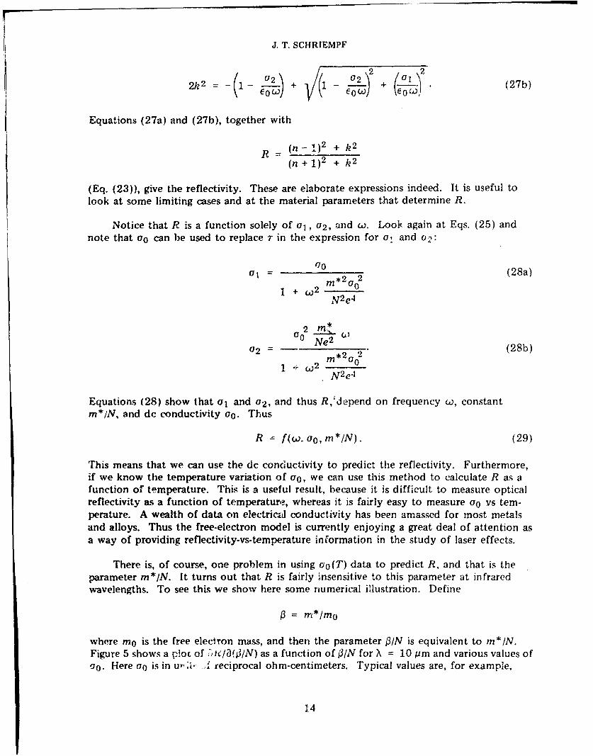
(Eq. (23)), give the reflectivity. These are elaborate expressions indeed. It is useful tolook at some limiting cases and at the material parameters that determine R.

Notice that R is a function solely of a,, 02, and w. Lool again at Eqs. (25) andnote that o0 can be used to replace r in the expression for o, and 02:

U07 *2 2 (28a)

1 + W2 m'00N 2 e4

Ne2

02 *2 2(28b)

N 2 e4

Equations (28) show that ul and 02, and thus R,ýdepend on frequency W, constant

m*/N, and dc conductivity c0. Thus

R -= f(w. Oo, m*IN). (29)

This means that we can use the dc conductivity to predict the reflectivity. Furthermore,if we know the temperature variation of 00, we can use this method to calculate R as afunction of temperature. This is a useful result, because it is difficult to measure opticalreflectivity as a function of temperature, whereas it is fairly easy to measure o0 vs tem-perature. A wealth of data on electric~il conductivity has been amassed for most metalsand alloys. Thus the free-electron model is currently enjoying a great deal of attention asa way of providing reflectivity-vs-temperature information in the study of laser effects.

There is, of course, one problem in using o0 (T) data to predict R, and that is theparameter m*/N. It turns out that R is fairly insensitive to this parameter at infraredwavelengths. To see this we show here some numerical illustration. Define

0J = M*/mo

where m0 is the free electron mass, and then the parameter O/N is equivalent to mn*/N.Figure 5 shows a pioc of Tu13•,/N) as a function of O/N for X - 10 pm and various values ofu0. Here oa is in u-ri. _, reciprocal ohm-centimeters. Typical values are, for example,

1.4

NRi. REPORT 7728

1 " - cm- i v l(-2.3 cm: for aluminum. Then the value of aI?Ia (01N)is: ;.hout 7.2X 102() cm- If we take a 10'/( error in l/'N we got

OR A(01N) = 7.2 X I0')2 X 10-24

o191N) (3N -72

W( = 0.00072.

Since for thesse values R = 0.97366, the change in R? is only about 0. 1%,. We can obtainqtune good predictions by the Drude-Lorentz model using the experimental values of o0and the moist simple choice for O/N, namely one free electron for each valence electronper atom in the metal, and PJ = 1. For alloys, it is sufficient to choose the major con-stitu(ent of the alloy. For example, with stainiess steel we choose iron, or two electronslpet atolin, to compute N and hence ikiN.

a0Z2

102 '

a020

C, 1 0-

10E ' \0 1WAIF NUMBER= 103 Vcm

00MiCRo. S)

a0 2 0ý2 10 22 10-ý 0-2

Fig. 5 Sensitivity o' to tht parameter

Figures G and 7 shuw the predictions of the frtee iectron theory for a variety of1metals and some compari-vol to ec perimental data 1:31 . The abrupt change when themetal molts is caused by the abrupt change- in the 0 conductivity. Notice in (he corn-l)arison to data that aluniinum films givv values cl-..-ý;t to the theory. This is probablyhbcause they prevnent th(- best surfaces. Diefects, oxide layers, etc., tend to trap thc inci-(lent radiatii ionIWId (cause they real surface to absorb more radiation than the ideal surface.Thvwse graphs are in terms (cf absorptance, which is the experimentally measured quantity,and, since metals aite opaque, uI 1 -I, which is correct for specular reflection at nor-mal incidence from an opaque sibstance.

oif

09- 304 STAINLESS STELL

081-

07

'• 04ý•

o 1ALUMINUM03" (POLISHE ! -

02[ 8002I! ALUMINUM0•0 (FILMS)

U 100 200 300 400 500 600 700 800 900 1000

TEMPERATURE (*K)

Fi"g. 6 -'Temperaturi, de),'.rdfdo(. tri tihe a'liorl-tance atl 10.6 j.

for aluminum aid stLiiiless steel

Let. us relturn to the expressio:is !o- n andt h to look at some limiting forms and thusshow how th,!se complete expression~s reduce to simple re!ationships. RIememher that It(Eq. (2 3 ) i' determined by n and he (Eqs. t27), which are in turn obtained from the deconductivity arid nzeIN (Eqs. (28). The variation of n and i? with wav'1ength is; shown inFig. 8 for a lypical good 'onductor like aluminum or copper at .,oom temperature. Notethat at long wavelengths n = 1h. We can derive this by using Eqs. (25) for ui and 02 andnoting that bs w -, o, u1 I I00, and o2 -- o0(yr. by substituting these into Eqs. (27) for

a and 1, we can readily snow that

I .hi2o (30)S2( 0 (,

This is called the llagen.-Rthen, liu,,t. Note that n is very large. Under these conditionsalgebra can he used to reduce Eq. (25) to

n+I

orR

Il

16

NRL REPORT 7728

ZL 012-

o - 304STAINLESS STEEL F

< 010-

- LIQUID-PHASE ABSORPTIVITYUjX 008- A I ALLOY -3.0 Cu,0.99 Si,,, 0.15 Fe,0.05 Zn,0 0.02 Ti

> 006 -I.-

o t

S004-A- - AAu 1 I

zz A L LOY"U Cu

cr002CU

-J

0 100 300 500 700 900 1,00w 1300 1500 1700 1900TEMPERATURE (°K)

Fig. 7-Free electron theory predictions of absorptivity of several metals at 10.6 p.The open symbols indicate the molten state.

WAVE LENGTH (MICRONS)

103 1000 100 10 1 0.1

1 02 2AGEN-RIJBEN1,o o ,o o ,.

100 ' IO ' Q

10 0o \0 \SP/N • Id6 3 cm3

1O-1 --

10-2 _ i I I I1o0 101 102 .03 104 i05

WAVE NUMBER (crm)

Fig. 8--n and h as functions ofwavelength (ljef. 3)

17

and Eq. (30) can h, substtktited for n to gt,t

This is tht 1lagen-Rubetis reflectiviiy.

We canl also comment on the skin ,lepth. We have, at long wavelengths (w, -• o).

27' 00

This can be rewritten as

(,32)

Equation (32) is the common expressi n foi skin depth used at long wavelengths.

Finally, we see from Fig. 9 that n and I? reconverge at short wavelengths. 'I his iscailed the plasma resonance- To see this, oi - must look" at the behavior of n and k over alarger spectrum. We have already discussed th,! long-wavelength limiting behavior of n and

h. This is the ilagen-Rubens rc.gion, wherte n - k. At short wavelengths, it is easy to show

from Eqs. (281 that

N~el

I?l ý20 (i(k

Ae 2

U2__ II.WAVE LENGTH (MICRONS)

Io 0O 100 10 1 0.1i0 3

1. HAGEN RUSENS

LIMIT nzik

0I -

orO o 3YT'I -n -- AS A -- 0

0

Ioe .k " 0 AS , - 0

10, 1 ~ d o1 0 0 I0 1 ' O. 10 3 le 10 •

WAVE NUMBER (Cm-,)

F'itg. 9 -t? and( k ais funlt'llS o i w;IvetlelIgttll

18

NRL REPORT 7728

Thus Eq. (27) can be written, for large w, as

n2 = 1 (33a)eom*W

2

k2 = 0. (33b)

Now the plasma frequency is usually defined from Eq. (33a) by setting n = 0 to yield

2 Ne2 (34a)Ep- 0 m, 3a

and thus

2

n2= 1--I (34b)

We see, then, that at very high frequencies the free-electron model predicts a transparentbehavior (k = 0) and the index of refraction approaches that of a vacuum. The transitioto this transparent behavior takes place at the plasma frequency, and it is a fairly abrupttransition, as Fig. 9 shows. In fact, some texts call this transition the "altraviolet catas-trophe." Note that at w near wp Eqs. (34) and (33) are not valid. For these frequencieswe must use the full expression. If we use again the values of ao = 105 2-lcm- 1 and0j1N = 10-23 cm 3 , which are appropriate to a good conductor like aluminum at roomtemperature, the refiectivity looks like Fig. 10. One can see that, in terms of the reflec-tivity, the transition is very abrupt, indeed.

R

1.0

0.8 "0.6 HAGEN-RUBENS

PLASMA FREQUENCY

0.2

0.0 -I I I I1000 00 t0 I 0.1

.4-,---X (EL)

Fig. 10-R as a function of wavelength

19

J. T. SCHRIEMPF

The optical reflectivity of real metals is, as we have seen, in reasonable accord withthe free-electron model at wavelengths in the infrared. The surface, however, must benearly perfect for the predicted reflectivities to be achieved, and, of course, as the wave-lengths approach the visible region band effects become important and the reflectivityshows rapid -Actuations with frequency. The absorptance of a practical metal surface isstill largely a~i empirical matter. For high-power, continuous-wave radiation by a CO 2laser, some data are available, but very little information on absorptivity as a function ofsurface temperature under these conditions is available. Shown in Table 1 are room-temperature absorptances for a few materials.

Table 1Room-Temperature Absorbtances of Aerospace

Metals and Alloys at 10.6 pm for Various SurfaceConditions and at Normal Incidence

Meta or__ Surface ConditionMetal or _______ _______ _______ _______

Alloy Ideal Polished As-Received Sandblasted

Al 0.013 0.030 0.04 0.115

±0.02 ±0.015

Au 0.006 0.01 0.02 0.14

Cu 0.011 0.016 0.06

Ag 0.005 0.011

2024 Al 0.033 0.07 0.25±0.02

304 Stainless steel 0.11 0.4±0.2

Ti Alloy 0.65(6Al, 4V) ±0.2

Mg Alloy 0.06Az-31B ±0.03

Data on the reflectivity of a metal during actual irradiation by a laser beam is quitedifficult to obtain, although this information is central to the problem of laser-materialinteraction. One classic experiment along these lines was carried out by Bonch-Bruevich,Imas, Romanov, Libenson, and Mai'tsev in Russia in 1967 [4]. They surrounded theirspecimens with a sphere to monitor the reflected radiation, as shown schematically inFig. 11. The output of the photodetector is proportional to the reflectance of the spec-imen. Some of their results for steel and copper are shown in Fig. 12. The laser pulse(Nd: glass laser, 1.06 jum), with a peak power density of the order of 108W/cm 2 , isshown as a broken line. As time passes, of course, the laser pulse heats the surface andthe reflectance decreases. An especially interesting feature of these data is the shoulder.The author has suggested that this leveling off is associated with the surface reaching themelting point and pausing at that temperature while the thickness of the molten layer

20

NRL REPOItT 7728

PHOTOMETRIC SPHERE

LASER____________BEAM

(7. TARG3ETO

I PHOTODETECTOR

Fig. 11 -Schematic representation of Bonch-Bruevich experiment

1.0I.O'

SLASER POWERS0.8 PULS

0.6

-J Iw

wz 0.4- STEEL

w /COPPERLL.

I 0.2

l//\

/\0/ I I I LL ,h.

0.2 0.4 0.6 0.8 1.0 1.2TIME (QLS)

Fig. 12-Reflectance of steel ar.o copper duringirradiation by a laser beam (from Ref. 5; copy-right 1969, Clarendon Press, Oxford, England.Used by permission of J.C. Jaeger).

21

J. T. SCHRIEMPF

propagates into the solid. In short, order, however, the molten layer begins to heat upand the reflectance continues to decrease. As the power density of the laser pulse reachesits peak and begins to fall, the surface temperature can no longer be inainuained, and asthe surface cools the reflectance begins to increase again.

3. THERMAL RESPONSE

3.1. Introduction

One of the most important effects of intense laser irradiation is the conversion ofthe optical energy in the beam into thermal energy in the material. This is the basis ofmany applications of lasers, such as welding and cutting. We shall summarize here thisthermal response. It is basically a classical problem, namely heat flow. In the usual man-ner, we shall seek solutions to the equation which governs the flow of heat, namely

PC- -T K - +- K- I + iK - + A. (35)Tt 3x 7 \3ýx a/ (~ ay az

We use here p for the density, C for the specific heat, T for temperature, I for time, andK for thermal conductivity. A is the heat produced per unit volume per unit of time.In Eq. (35), p, C, and K are considered functions of both position and temperature, andA is a function of both position and time. In effect, the equation is a simple statementthat the rate at which heat accumulates in an elemental volume dxdydz is equal to thenet flow of heat across the faces of that volume plus the rate at which heat is producedwithin the volume.

Thus thermal response studies consist essentially of two parts. Fik'st, one needs toknow the rate and source of production of heat by the laser, which yields A. Then onesolves Eq. (35) subject to the boundary conditions of the situation of interest. This canbe a very elaborate task and frequently can be done only with the aid o.f a computer.There is a great deal of effort among workers in the field of laser effects to develop anall-inclusive computer program to solve Eq. (35) for every possible situation. However,the solution to Eq. (35) can be no better than the knowledge of A, and, as we shall seein later sections, it is often very difficult to establish A with any precision in a laser-material interaction situation.

3.2. No Phase Change-Semi-Infinite Solid

Let us consider first the most simple situation. Let the laser beam be perfectly uni-form over an extremely large area, so that we have a one-dimensional situation. Assumealso that the material parameters are temperature-independent and that the solid is uni-form and isotropic and of semi-infinite extent (Fig. 13). Finally, assume that there is nophase change; the rate at which energy enters the material is not sufficient to inducemelting or vaporization.

First rewrite Eq. (35), using the fact that p, C, and K are constant:

32T 1 3T A (36)3z 2 - 3t K

22

NRL REPORT 7728

UNIFORM LASER SEMI-INFINITEBEAM SOQL I

z:O Z ---- 0.

Fig. 13-Uniform irradiation of a semi-infinite solid

Here we have introduced K = K/(pC), which is the thermal diffusivity. Let us adopt theconvention that T is measured with respect. to the initial (or ambient) temperature of thematerial. This is possible because Eqs. (35) and (36) define T only to within an additiveconstant. Then we have as a boundary condition that T - 0 as z - oo. The boundarycondition on the front face (z = 0) depend-. on what we assume for radiative and con-vective losses. It can be shown that, for most cases of interest, the rate at which thelaser creates heat at the interface is overwhelmingly larger than convective and radiationlosses, so we ignore them for the present calculation. Thus the boundary condition isthat there is no heat flux at z = 0, that is,

K aT =O 0.

Now consider A. Denote by I the power density of the laser radiation at the sur-face; the dimensions of I are power per unit area. The power density of the radiationtransmitted to the surface is I(1 - R). Then the power density as a function of z is

F = (1 - ýP)Ie-47IkzfX. (37)

This follows from the fact that the energy in the electromagnetic wave goes as '2. Nowto get the power transferred per unit volume, consider elemental volumes of length dzand unit area:

A= _)F = (1 - R 47r e-47Tkz/X . (38)-az =xi •(8

The minus sign appears because VFlaz is the power per unit volume lost by the radiationand A is the power per unit volume absorbed by the material. Finally, we define theabsorption coefficient

4= 1rk (39)

23

J. T. SCHRIEMPF

which is, of course, 1/6, the skin depth. Thus

A(z, t) = (1- £R)I(t)ae-Oz (40)

where we have included the possibility of I varying with time.

So the equation to be solved is

a 2T 1 aT (1- R)I(t)a e-Oz--- - =- - (41)az2 KC at K

In keeping with our assumption of temperature-independent thermal parameters, we as-sume further that R is independent of temperature. Equation (40) is valid for temperature-dependent ! and can be used to give A (z, t, T).

For metals, ot is a fairly large number. As we saw in Sec. 2, k is of the order of 100at X = 10 prm, so that (x is of the order of 106 cm- 1 . Hence the absorption occurs in avery narrow layer at the surface. It then becomes more convenient to seek solutions of

32 T 1 = 0 (42)aZ2 K at

subject to the boundary conditions that T = 0 at z = oo but with a specified flux into thesurface at z = 0, i.e.,

-K ) = (1 - )I(t)v-Z.0

or, with the definition

F(t) = (1- R)(t), (43)

-K z) = F(t). (44)z.0

First examine the case of F = F0 , a constanL. This is appropriate to irradiation by a con-tinuous laser, given t'mperature-independent material properties. We note here only thesolution, for many excellent texts on heat conduction can be consulted for the details [5].

The solution to this problem is

2F0 TT(z, t) = K ierfc [z/(2 ,/Kt)] (45)

or

T(z, t) = e-Z2 4Kt 2 erfc -z"(2VIt]

24

NRL REPORT 7728

The functions which appear here are error functions, and it is useful to summarize someof their properties and definitions. (See Ref. 5, Ch. 11.)

The error function is

erf(x) 2 J0 eC\7r

erf(o) 0, erf(o) 1, erf(-x) -erf.(x).

The complementary error function is

erfetx) 1 - erf(x,) 2i e-'

"The inregral of the (complementary error function is

ierfc (x) j erfc (ý') dA

or

1 2in-rf(x W eX x erfc (x)

__rfc_(x) __i- e x + x-__t_ W

Some derivatives are useful:

•J erf Ix i erfe (xj 2 "dxa ",ix x-

iJ2 erf•x) )2 erfc W(.x2bx 2 ,ITr

0 4.rfe. Ix)--- -- 7e-fc- (x)Ox

i i' ,erl" ix) 2 7 2

~x~ 2 /- C

Now we can show that the houndary condition is satist ed. Using the first form of Eq.(4F5 yillds

" 21-" v'rdlerfcfz/(2v' ,I)l 1-x 1 / J 2 ,5v7

25

.1. T. SCIIRIEMPF

and since erfc(o) 1,oT') 1"0

L -)z

O(ne can also show tiat Eq. (45) satisfies Eq. (42).

We can us,- Eq. (45) to show what the front surface temperature behavior is, underconstant irra'ihation, by setting z - 0 so that

T(o, t) ( 4('

'.,s an illustration, l0t us calculate the time required to raise aluminum to its meltingpoint for ai power density of 5 kW/cm 2 -

K = 2.3 W/!cm 2

K 0.9 cm 2 /s

"Fmp,,; -- 600"(

T : Tm,.it -- Trom = 600"C

F0 (1 - "'1

1 - *)" 0.0-1

0.0.1 X 5X 10:1 = 200 W!cm 2 .

"lThn t (,rK 2J' 2 )1(4, F 2 i) yields t 4: 42 s. IIn practice, it is very diffhiuit to melt extremelythick slahs of aluminum A.ith even a high-power laser, as these calculations suggest.

Equation (45). although derived for a very simple case, descrihes man, very importantfeatures of tiiermnal response to lasers. First we shall define the diffusion length, which isuseful in that it permits a wide variety of order-of-magnitude calculations to he madIe. Thtthermal diffusion length 1) is defined as.

1) 2./•. 7

Strictly speaking, the thermal diffusion length i.i defined as the distance required for thetemperature to d1 up t; 1,;, of its initial value and depend:: soimiwhat on the geometry andthe boundary condition. For most purposes it is sufficient iimply to take it as definedby Eq. (17J. 1,ook'ng at our solution (Eq. (15))1 for example, we see that

2 G

N R L itEPOrT 77-,28

2,F r- 1 1)}T(D, V (0.1573)

From Eq. (4o),

"T(I'), t ) , 1 - 0.1573 73-/ .

Thus

T(D, t) - 0.09 T(o, t) (48)

in this case, whereas (lie) T(o. t ) •- 0.37 T(o. 1). Referring to our example of irradiatingaluminum for 412 s to reach the meiting point, we note that the diffusion length at thattime is given hy

) = 2 vU. .9 ,-4 2 • 12cmr,

and, by Eq. (4h). the temperature at distance D into the material is 0.09 x 600, or about50'C above ambient.

Nov. let us illustrate the solution (Eq. (45)) graphically (Fig. 14). For conveniencerewrite the equation by introducing 1) 2 \f/7-1 and by reducing it to the error functionerf, so that

2I} - -, 2'/1) 2 z zi.... = .(z D )Ki2/- 2 2j

108

e-• 2 0 9953

eni Icn ] I(j (. ~~cIy

S4

o2 - 1 - - 1 1_

05 I IC 21 2L5 30x

Fig. I I -'Th t.rrr)r func ion

27

,J. "'U. sCIiE.,Pp

Now let T z/i), and

'¾. t=f -0-K- r [/ -7i + il erf(r/). ('19aI

or, equivalently in terms of ierfe,

T(Z, 1) ierfc (rq) (. 9h

Finally, we define a dimensionless temperature 0 TKI(,O)), so that

L = ierfk (1)j. (49c)

Thus the plot of the integral of the complementary ,rror func;ioin here is ti.' graph oftGe solution to the problem of constant heat flux on the surface of a semi-infinite solid.

Now, although the graph of Eq. (49c) (see Fig. 1 5) represents very succinctly thesolution to our problem, it does not really snow how the temperature varies as a functionof position and time. For this purpose it is useful to look at the temperature profiles forvarious times and see how the profile chtngs with time. These curves can be generatedquickly from U ierfc (rT) by recalling th" de, ientions of 0 and 7, and writing them in thefoliowing form:

T = F (50a)

z 2 vf', v T ?.7 (50b)

t06 } -

,er!C (j) ' O5E4?II) 00502

IerIc {() Z eC .. !

01I

JJ

0 02 04 06 08 10 2 14 ,5 18 20X

Fig. 15 -'The integral of .t complimentary error fu iction

28

NRL REPORT 7728

Thus, at a given time the 0 = ierfc (17) curve scales according to Eqs. (50); the basic shapeof the curve is unchanged, but it is stretched one way or the other depending on theparameters, and this stretching progresses in time as VT The case of aluminum is shownin Fig. 16.

SEMI-INFINITE SLAB OF ALUMINUM IRRADIATED AT ? 0EBY 200 W/cm 2 OF ABSORBED LASER RADIATION

(I = 5 kW/cm 2 1 - R = 0.4)

600 K = 2-3 W/crn degX = 0.9 cm 2 /S

I--z X DENOTES DIFFUSION LENGTH D 2 rK7M 500 42 s

>o 400

w20Scr-S300I-

'2200- 0SC-,

-100

0

0 2 4 6 8 10 12 14 16 18 20 22

; (cm)

Fig. 16-Laser-induced temperature rise in aluminum as a function of depth

We can also look at the variation of temperature with time at a fixed position. Thevariation of the surface (z = 0) is simply T(o, t) - t as Eq. (46) shows. Whereverz/(2 %/'I) is very small, the temperature variation will approach \T Thus, at any posi-tion T : VTtat sufficiently large t. The temperature-vs-time profiles at fixed position fortimes such that z/(2 •V_-•) is not small can be calculated, of course, from Eq. (45). Someresults for aluminum, with the parameters used above, are shown in Fig. 17. Notice thatat z = 10 cm the temperature profile is far from the "long-time," or vNT, behavior even at40 or 50 s, whereas the surface has already begun to melt.

We now turn to some order-of-magnitude arguments. One such argument can beused to estimate the power-pulse length combination which might be expected to yieldsurface vaporization. Consider a laser pulse that has the simple time behavior shown inFig. 18 and uniformly irradiates the surface of the material. The pulse length is tp andthe intensity is such that, combined with the reflectance, the absorbed power density isF0 . Again we assume that the optical energy is absorbed in a very thin layer at the sur-face. Let Dp be the diffusion length associated with the time tp. The question iswhether a significant amount of surface vaporization will occur before the pulse ends.One approach would be to use Eq. (46) to calculate the surface temperature at the timetp and compare it to this vaporization temperature. However, this would ignore the in-fluence of the latent heats of melting and of vaporization, which have an important in-fluence. We shall discuss thermal flow with phase changes later. For the present purpose

29

J. T. SCHRIEMPF

800-

Uj

*-0700

e -

4

w

Cr

300SEM r I5 NIm

SOLI4A'p

03

NRL REPORT 7728

we can include them by considering the energy required to melt and vaporize a portionof the material. The key is to estimate what thickness of the material is involved, and inthis order-of-magnitude argument we simply use the thermal diffusion length for thisthickness. Thus we set the criterion for vaporization as

D--p- >_ p[Cs(Tm- To) + Lm + CQ(Tb- Tm) + Lj]

where p is density of the material, Cs and CQ are the specific heats of the solid andliquid, respectively, Tm is the melting point, Tb is the boiling point, and Lm and Lb arethe heats of melting and vaporization. Notice we are ignoring differences between thesolid and liquid for density and conductivity, as is appropriate in this crude argument. Ifnumerical values are checked, Lv, dominates the expression on the right side of the inequal-ity. For example, for aluminum Lv = 10,875 J/g, whereas all the other terms contributea total of 3.046 Jig. Since the argument is crude, then, one usually takes

F0 tp- > pLyDp

as the criterion for vaporization by a pulse. Since Dp = 2 VW' , we have

2 V• LvpF0 _> approx vp (51)

Some calculations based on Eq. (51) are shown in Fig. 19. Most metals fall in the bandindicated. For a given pulse time, at power densities greater than the band indicates,vaporization effects would be expected to be important. Some useful thermal constantsare included in Table 2.

S0sE

0. VAPORIZATIONz

L.J> 107t:

Z

CrW

0 NO VAPORIZATIONt•

0

I I ti39 J 155 j(53 10"1PULSE `-, 'V 'Is)

THE BAND INDICATES WHERE Eq. (51) LIES FOR MOST METALS

Fig. 19- Power density--pulse time criterion for vaporization

31

J. T. SCHRIEMPF

E - ! II.. r4 ~s 2 - - i6 6 E

*4 X

* 1z

5.4l 4"__

c4,

m c

oc

flc0n'

32'ae'

NRL REPORT 7728

In deriving Eq. (51), we have been seeking the power density required, at a givenpulse length, for a thermal layer to be vaporized. The same expression, of course, tellsus the pulse time at which vaporization becomes important for a fixed power density.Rewriting Eq. (51) gi- s for this time

K 2 2Tvap 7

tp > approx TF2 7 (52)

Let us compare this to the time required for surface vaporization to begin. We do thisby using our solution for heat flow in the semi-infinite solid for the surface (Eq. (46))and solving for the time at which the front surface reaches the vaporization temperature:

Tvp-2F0 ta

or

tvap - _ Vaptrp=4 F02

Thus, at tp = tvap this calculation would predict that vaporization at the surface begins.For example, at F0 = 106 W/cm 2 , vaporization begins at tp - 10-5 to 10-6 s, depend-ing on the metal. On the other hand, for a thermal layer to be evaporated requires, ac-cording to Eq. (52), tp ý- 10-3 s. It turns out that both estimates are useful. In a latersection we shall discuss features of a more correct treatment, which accounts for boththe heat of melting and the heat of vaporization in the dynamic situation of propagatingsolid-liquid and liquid-vapor interfaces.

3.3. No Phase Change-Slab of finite Thickness

Let us turn now to a treatment of another geometry which can be useful in practicalcases, namely irradiation of one surface of a sheet or s!ab of finite thickness. Let the slabbe taken as infinite in extent in the x and y direction, and let the laser irradiation be uni-form over the entire surface z = 0. Thus we again have a one-dimensional situation, asshown in Fig. 20. The thickness of the sheet is taken as £, the absorbed power densityas a function of time is F(t), and we again assume that the radiation is absorbed in a verynarrow layer at the front surface. The equation we wish to solve is, then,

a)2 T 1 aT

Jz2 T at

with the boundary conditions

-K = F(t)

-K 0.) O.

33

J. T. SCHRIEMPF

F (t

Fig. 20-Irraciati(t n ()f a slab of finite thickness

The second boundary condition states that" -he rear surface is insulated. We shall look atthe consequences of this assumption a iittl.e later.

As we showed for the semi-infinite slab, the solutions turn out to be elaborate.Turning to the special case of F(t) FO, a constant, the solution is

T(z, t) = FO-t {3(+- z))2 Q2 2 \ (-ý1)" CK1 2 1T2 1IQ2 Cos(nT z)[KV K 62 2 . n2 [ 9 KLn=I!i (53)

We can check that this satisfies the boundary conditions:

a T_ F0 9 f~Z) e-I (-1)jý ei silln F2rn=1 .J

Now sin (nirT) =0 and sin (0) =0, so the 1 term vanishes at both z =0 and z Q,and

FO

= 0.

Similarly, the thermal diffusion equation is satisfied, as the reader can verify.

Let us look briefly at this solution. It consists of a linear term in t, together with a"correcting term," which can he plotted as shown in Fig. 21. In other words, what isplotted is the term

34

N It , ItEPOT IVY8

03 .... 0.3

0 02 . . . .

0' ( I- 4- ---' - -41 0005

0 -0005---- -

-0i

u 0.2 04 06 0.8 1.0

NOTE THAT v( z< k. THE NUMBERS ON THE CURVES ARE VALUES OF /12

F g,. 21 - i funotion (if I /' (Ref. 5, p. 113)

I' ~'1:- .- .j ( ) . .. .

( i 2 ( ;T 2 , .- . n1 2

Let us examinine .- f special case:s. At z = 0, for cxan,plo,

P.? K r, 9K•2 '2 t i (5V)

lVe can rewrite this as

"l,, t) KF + K oK V

Now T at a fixed value of 2 is a function of Kt/Q 2 . It 'I 'I , we can write

l1,o

T"o, 1 (7? + J'z. o(71)). (55)

;35

__L.

J. T. SCHRIEMPF

Figure 22 shows how T, depends on ,7, for z = 0, and was taken from the previous graphof T, vs (1 - z/Q) (Fig, 21). Note that at small 77, i.e., at Kt << Q2 , P• 0, so that thefront surface initially heats up linearly with time, as

F0KT(o, t) M P t.()

04L

03-

0.2

ot

0o 0.1 0,2 03 04 05

'7-

Fig. 22- - at z 0 as a function of 77

For large t values, or Kt >> Q2, 0z=O approaches a limiting value of about 0.33. Thus atlong times

T(o, t) = -- + 0.33 , t >> Q2. (57)

Here again we see linear behavior, but this time there is an additive constant. If we havea very thick slab, we should get the same result as our previous solution for the time toreach 6000 C on the front surface of aluminum with an absorbed power density of 200W!cm 2 . It turns out that the limiting form of Eq. (56) is not correct because it ignores thebehavior of ý'P= 0 (77) at small r7. It. is necessary to use the full expression. Thus

77 + 1Z=0(7?)= F0-

Assume that Q = 100 cm, since we know from our infinite-slab solution that the diffusiondistance is 12 cm at T = 600°C on the front. Thus

2.3 X 60077 + J z=O{T7) 200 X 100

Reading very roughly from the graph of Dz=o vs 77 gives

36

NRL REPORT 7728

t? : 0.004 at i 0.065.

Thus our solution is

'a

77 - 0.004 =

which gives, since K - 0.9 cm 2/s, a time of about 44 s, in reasonable agreement with thesemi-infinite-slab solution.

Now let us turn to a consideration of the rear surface temperature. For this case,z = Q, so Eq. (53) becomes

Kot K0 6 .2 k- (-1 )fl Kln ~ /2

T(V, t) - F0 tK + KF0 Q [ 2 L _ e-__ n27r2t/Q 2

or, introducing 77 as before, we have

T(Q, t) = K (7 + j"z--(7,))K

Comments could be made here for the rear surface temperature, and they would be simi-lar to those we made for the front surface temperature. It is interesting to compare thefront surface temperature to the back surface temperature. This has a simple form forthin sheets, where Kt/Q 2 >> 1. By referring to the graph (Fig. 21) of T vs (1 - z/Q), onecan read off values for j'-z=V(o) and :J~z=o(O), and thus

T(o, t) - T(Q, t) ' 0.5K

for

at/V 2 >> 1

Notice in Fig. 21 that the limiting values are approached rapidly; they are nearly realized

by the time at/2 2 = 1. As a numerical illustration, if we have 0.3-cm-thick aluminum,

T(o, t) - T(Q, t) - 13 0 C

For the same numbers we used above. This situation, with the two surfaces heating atthe same rate but separated by 130C, would start at a time of the order of t - 22 /1c0.1 s. At this time the front surface temperature is about 35 0 C.

Let us turn now to a different sort of heat input. So far we have been discussingcontinuous irradiation. Another simple case, which is a reasonable approximation undercertain conditions, is that of a laser pulse which is short enough to be treated as a deltafunction. Take again a slab of thickness 2, and assume that the energy is deposited in avery thin layer near the surface. F refers, as before, to the fraction absorbed by the ma-terial. The laser power density, that is, must be multiplied by the optical absorptance. Inthis case we solve the thermal diffusion equation subject to the boundary condition that

37

J. T. SCHRIEMPF

-K-iT _-K-iT 0,

with the stipulation that there is an instantaneous release of E 0 units of energy per unitafea in the plane z = 0 at time zero. This type of problem is discussed in Carslaw andJaeger [51 and is most easily solved by Laplace transform methods. For our presentpurpose we quote the solution

T(z, t) = E0 1i + 2 N cos(n z e .K121T2t/Q2 (58)

In Eq. (58) we have introduced E0 , the energy per unit area in the pulse. Thus,

f00Eo 0 F(t) dt .

'o

For the case under consideration, F(t) is considered to be a delta function.

Equation (58) is the basis for a scheme used quite frequently for the measurement ofthermal parameters [6]. This scheme consists of using a thin sheet of the material to bestudied and irradiating uniformly one surface with a very short laser pulse while monitor-ing the temperature rise induced on the back surface. If one knows E 0 , and if the as-sumptions of no heat loss are valid, the experiment can yield values of both specific heatand thermal conductivity. One adjusts the pulse energy, and hence E0 , so that the in-duced temperature rise is smail. In this way the values of specific heat and thermal con-ductivity are representative of essentially the ambient temperature of the material.

To see how this is applied, rewrite Eq. (58) for the back surface, z = Q:

T(Q,t) 0 11 + 2 n (-1)n ecfl21r2!/•2. (59)

If we introduce a characteristic time t, = .2 /K~r 2 , Eq. (59) looks approximately like thecurve shown in Fig. 23. Here we ',ave also introduced a characteristic temperature Tc =Eot<iKQ and plotted T/T, vs t/tc, or

00T - 1 + 2 - (-1)'e-n2tltc (60)TCn=1

Essentially the experiment consists of monitoring the temperature as a function of timeand fitting it to Eq. (60). This can be done quite readiiy. First, the long-term tempera-ture rise T,, yields the specific heat because

-=1

T3

38

NRL REPORT 7721

1 0

0 1 2 3 4 5 6

037

t/tC

Fig. 23 -- Nornalized back surface temperaturo res.ponsw toa delta function heat pulse

and, on substituting for Tr,,

or, since x - K/pC,

Thi,. technique of measuring specific heat is, of course, not ufnique, to pukbed lasers It is.sofit'tones referred to as the slat, calorimeter. The accuracy of the method depe-nds onknowing K<, which is frequently difficult to ascertain with laser radiatio,. In siine ap-pic'ation. Eq. 161 ) is used to calculate Eft, the energy actvally absorbe-d from the laserpulse, by using materials o. known specific heat.

The pulsed laser measurement teclinique is especial y suittid to defermining theirnaldiffusivity. 'L'he magnitude of the back surface temperature rise depends, as we saw, onthe energy which is coupled into the material, and this may be difficult to kaow withany pre(ision. H[owever the time dependence of the hack surlaca temlerature is mndependent of th' energy input and is controlled only by the diffusivIty K. A simntlle wayto derive ic from a temperature-time profile can lie seen from Fig. 23- (ie measures the

time required for the mncasured temperature response to reach some fraction, say one-half, of its limiting value. Let us call this time Il. It can lie shown numerically (61from Eq. (60i that

is satisfied when

39

J1. 1'. S3CRIRENIPP

t12I, 1 .37 .

Usin ~ ~2 /j(772yields

1.37 V2 (62)7T 2 1 ]/2

Tfhus a measuremenlt Of t 112, together with the thickness of thle specimen, immediatelygesthe thermal diffusivity. If one knows EnI this experiment g~ivtes. vel-ies of both the,

s;pecific hneat and the diffusivity. ý'nd hence if one knovis the density p thle experimentgives thle thermal conductivity.

This technique has heen apphed often, at rather high temnreratures. usually inl the1)0O0ý'( range and above. At these temperatures steady-state methods of measuring thlethermal conductivity are difficult to apply hecause radiation losses are so large. In thelaser flash tech[Lique the radiation loss goes like 'j' T61 where 'To i.s the starting orambient temperature, establiished by, say, a furnace, and 7' -is defined above. Thisradiation loss canl h- ~i.ddle quite smnall by adjusting E0 so that TIL- is only a few degreeslarger that, 'i Since 0the precise value of E(0 is difficult to estahiish, these experimentstypiciilly mneasure anly * e thiermial diffusivity, not thle conductivity.

A final remark Onl thle Lriterion0 for the applicability of Eq. (601 to slab) heatfi g con-cerns the limits onl the laser pulse' duration. No laser pulse is, of course, a true 6 fun-ction.Ouar solution WOUld be expected to be correct for la.;er pnlse tim-es which are short comn-piared to thc time it takes the hack surface to resp~ond. The response times are of theordcr of 1~, so wev have the criterion

or

p << k2 1(KrT2

C'alc-ulat ions Ahat include explilit ly the time dependence of thle laser pulsŽý 171 indic-Itethat our b-fu ction solution iin error by less than about 2% provide'1 that tG) is less thanei equal to about 4%/( of t,.. Some typical valuer: of 1, wvith specimens I mmn thick aregiven below.

K - i~r

(cM 2 /5j (inS)

AI lminum1 0.85 1.2Stainles;s steel 0.0 52,? 19d

'I ypecal laser pulse lengi h are about 1/2 to 1 ms for the so-called "ncrrnal mode"lasefs, and thus with I -mm-thick '-clr~mens thle technique would be fairly at-ckmrace forstainless steel but not very rood for aluminum., Thicker specimens, would hielp, hut thiswould mak 'e the rear surface temperatiir'' rise smalevr. If our laser p~ulse has, say, 20.l,'c.m2 in it and we use the 10(.6-pum absorptanco quoted e~arlier for as-rec-eived surfadces,tho vntttiipatod te1m-perature rises at the ;hack of the i -imm specimens would be as shov.nhe; o %.

40

NRL REPORT 7728

p C = E0 i'pCk(1 (J/c 2) ( g/c:m2) (J/g°(t) -c)

Al~mrinum 0.0, 0.8 2.7 1.05 2.8Stainless steel 0.4 8.0 8.0 0.628 16

We see dic need to use shorter laser pul:es hut with the same amount of energy. Anothersolution would he to carry cut a more detailed heat-flow calculation. Both tailoring ofthe- pulse shape and more detailed calculations are usually employed in current applica-tions of laser flash techniques IS1

3.4. Melting

Consider first the case of a seni-infinitt, slah melted, with instantaneous meit re-moval, as indicated in Fig. 24.

I]= Tm•/

Fo __ I /I SEMI - INFINITE

""FI MEDIUM

_ - , /-z:O z=Ut

1•'i• 21 -']rra(iid Ion ofs s-mo-iinnoilie I)o \'hh

illsta l('U.a ine -li rInmt jV

We solve this hy conAidering ours(-Ives moving i)rig with the interlace. But to dothis we have to reconsidur our heat-flow equation, which is

T)"1 1 /)7 -. 0(1z2 K d

Iecaull that this was derived by noting th-- rate( at which heat accumulated in an elementalvolume:

(jtP. C. 7 7-- K - 0() t (jz ,)z "

If the ned Urn is Ineving, an additional :,mounL. :,f heat pCI is. flowing in at rate V.So

41

J. T. SCHRIEMPF

-K "•T becomes -K - + VpCT.

"Thu.i, for moving media, the heat-flow equation is

C -K !T + VpC( 0ot oz do /

provided we are not generating any heat in the solid.

Thus

+T 27 0. (63)a ýt 2 bz

Se .%e can find at least a steady-state solution to tUe proble)m by basing our coordinatesystem at the interface and letting the material flow in at some rate to be determined.

Call the rate - 11, where U is a positive number. The solution will be

T' = TFre C'z/ ((34)

where K is diffusivity of the solid, 'Tr, is the melting temperature, and z' is the distance

from the melting front. That is, this is t.hv solution to

3T 52T ; IK -- , 0 U

ot ,)z ()z

as we (an verify. First, aJd'/It -- 0 because this is the steady-state prcbfile, or

K -1r • a-i' 0. (65)c .Oz , .2 D)z '

Of course ' - T/,• at z' - 0, and 7T -- 0 as z' - ,. is trivial to show, by differentia-

tion, that Eq. (641) is the solution to Eq. (65).

"Io calcuiate U, we use' energy balance. FL) must raise the material to T,,,, its neltingpoint (T,,,(' above• ambient). and then mf,!, it. 'Ilhus inl time 11, the energy put initothlic'kness A.z' (where U---Z'/al) VIust be giv~tI by

I--" Lp + C', p

or

l' 1= ,l, + C';, l . (6;6)

Thus wý' ,%t-•ritv, for the stAviidy-•tato, tempegtra.turet profile,

42

po1ii iiiiin i T i 0 i ibv aien i.adte n-it1bsinime Ihenrgpu i it( i

NIt , REPORT 7)28

-,,~ L- ,(67)

where Fo',[p(L + CT'I)j is the velocity of the melting front. This solution also would beappropriate to suhbniatioii, where L is then the heat of sublimation and Tm the sublima-tion temperature. Note that this is the scmi-infinite-slab approximation and cannot beused to estimate the time to penetrate a slab of given thickness.

Let us consider aluminum, with F 0 : 200 Wjcm 2 . Taking a more accurate value ofthe melting point than in earlier examples, T, -- F.40(C (the actual melting point of6600(. minus room temperature of 200C). If we put in the other values of the param-eters, T falls off a., shown in Fig. 25.

T= 6406-0.082Z'

640CR1 JOE SI(E ;CH

NOTE I/ePOINTAT-z' :12cm

- 320

0

o ll ,I0 10 20 30

Z" (Cm)

FiI4. 2-:-.'lno peraturv profile in alu iinium withilstantanoOUs melt retmvai I

As another illustration, consi(der !lexiglass. Plexiglass is rapidly eroded by 10.6-timlaser radiation, by a process that is essentially sublimation. Since it couples extremelyweHl ((I -- 1.0) and has a very low thermal diffusivity (K - 10-4)I cm 2 /s), it can be used to

make "hurn patterns" of the beam. That is, the depth of the erosion at a given point islinearly proportional to the energy density incident at that point. %Ve can understandthis by applying heat-flow cOncl)t, l.,Lt us apply EP(. (67) and interpret L as the heat oferosion. Since C z- 1.1 J/g-'(: and 'T,, - 200"C and L . 1000 Jig, for a crude ('a cula-tirn wo can ignore T7i J. 'Ihe' ensity is thout 1.1 gl/m:1. We tien have

T !- 200 e- 4FO

Since (U - 1, for a typical poNe-r density like 5 kW/'in,2 we hav' I0 = 5 X 103, so tlmt

T z- 200 eI j x ])404,'

Helnce tho temperature irofile is cof fined to an extremely narrow region near th,, vrodingsurface. The rat.' of e.rosion is, by Eq. (66) with C':, igo ured,

43

L,.. .

J. T. SCHRIEI'MPF

U - 4.5 cm/s.

Now we can see why plexiglass is useful for monitoring the beam profile, and whyit can pick up fairly fine structure in the boam. After irradiation for a time t the pene-tration depth is U't - (Fot)/(pL), and this should be large compared to a thermal diffusionlength D 1 2 N/-0 if the p.ttt.rn is to rot-,al fine structure_. Otherwise thermal diffusionwould "wash out" the pattern by distr'ituting the energy in a radial direction. Thus

2 \V-Kt<< ýLt -pL

For the numbers we used above at t z- 14 s, we have a depth of 1 cm. Thus

2 10_- X 1 0.1 mm << 1 cm

and w' see the criterion is well satisfied.

Let us look at a more complete poblem, namely melting by laser radiation of aslab of material. One basic problem is what happens to the melted material. (We willignore the vaporization question fur now.) There are two eases which are fairly amenableto numerical solution. They are the' "fully retained liqui"' cai,0 , in which all the liquidis presumed to v-tay in place, and the "full ablation" case, in which the melt is presumedto disappear magically as soon as it forms. The latter case might correspond to the pres-once of a heavy windstream which blows away the melt.

1,.m( king first at the full ahlation ci e, we have MIh situatton siown in Fi)g. 26. 7'2is the temperature in the solid, and the Iront surface at z = 0 first warms up to the melt-ing point T" (above ambient) and then begins to move to the right. S denotes its posi-tion as a function of time. When S = Q, the process Is over, and we call this time tf. We

denote by 1,, the time at which the front surface begins to melt. The field equation is

T I

F0 INSULATED BACK SURFACE

zrO z:S / z:1 2----

SOLID REGION, T T2 ( z,t )

Fig. 26 Fully ablated ca:se

44

NRL REPORT 7728

a22 1 3T 2=2 K2 at =0 for 0 < t < tf.

The boundary conditions are

K 2 aT)z = -F 0 for 0 < t < tm

SdSK2 - --F 0 + -pL- for trn < t < tf

z =S

K2 3Z = 0 for 0< t < tf.

The starting conditions are

T2 (z, o) = T20

S)t < f O

The above boundary conditions are nonlinear, and a solution in analytical form isvery difficult. This is due to the presence of the moving boundary and appears in thesecond boundary condition, which states that the bcundary moves at a rate dS/dt deter-mined by a balance between the heat of melting L, the heat input F0 , and the heat flowby thermal conduction.

One relationship must hold for this problem; it follows from energy balance. Thetotal energy put in per unit area is Fotf, and, since the material is simply heated to Tmand melted, this energy goes solely to those processes. Thus

Fotf = p(L+CTm).

This is convenient, for one can check numerical solutions. More important, it gives afirst-order estimate of the time needed to melt through materials by laser radiation.

Turning now to the fully retained liquid case, we have the following set of equations.The definitions are the same as above, except that subscript 1 now refers to the moltenstate, whereas subscript 2 is still the solid state (see Fig. 27). The field equations are

a 2T2 1 a T2 = 0 0 < t < tf (solid)aZ2 K 2 3 t

3 2 T1 1 aT1- = 0 tm < t < tf (liquid).

The boundary conditions are

45

J. T. SCHRIEMPF

T=Tm

F0 I INSULATED BACK

SURFACE

Z= X= S =1 Z- --

LIQUID REG:ON,T=T1 (z,t)

SOLID REGION, T=T 2 (z,t)Fig. 27 -Fully retained liquid case

K 2 3) = FO 0• t m

SO Fo tm t < tf

K I d' 1 - K 2 Z = -pL -- , tf

K2 ýTh2 =0 0 <t <t f

T2)z=s = Tl)z=s =Tm tr < t < tf.

The initial conditions are

T 2 (z, o) = T20

S)t < tm = 0.

Rather than discuss this problem in detail, we pass on to the more practical, althoughmore complex, case of vaporization. For the fully retained liquid case, suffice it to saythat the retained liquid has a shielding effect, and thi; causes the time to reach melting atthe back surface to be longer than in the ablated model. Some typical values of melt-through time for 0.2-cm-thick material with F 0 ; 2 kW/cm 2 are given below.

46

NilL REI'OtT 7728

,\hIlattlI Retainecd(s) (s)

A11 nliinmI_ 1.32 0..17statilless steel ,1.0 4.5

3.5. Melting and Vaporization

We present hert without derivation some result.s for the cuse of a slab of material,insulated ork the surf aces, subje, cted tro uniform and continuous irradiation 191. Theseare one-diniensional calculations. It is assumed that the inilt is fully retained until it-reacihes the vaporization temperature, where it disappears. Tlhen we Lave the case illus-trated in Fig. 28.

Fo LIOUID SOLID INSuLATED SACKSURFACE

I II

zO z:S 2 z:SI z:e z-

Fi- 2?8 Meltin did Vai)orii.ailn, wi.i fully ,.,it'i d Iiquid

"I • 2r, ,%, is the, position of the liquid-vapor interface and S! the position of the Solid-Iiqtuid interface. This probhlerm Iis been solved numerically at NKL, 191, and we shallshow sonic results. The asuin;t'tons art' that in ciach phase the thermal properties areindependlent of temperature. In the curves, the following definitions are used:

0]K.5 11 d

K•odld I

i ." (] - 'fmi(-s.o)io ,1

,17

J. T, S('IIRIEMPF

1, latcnl heat of fusion

subscript 0 ambient temperature

= LL,, with l,, the !ater heat of vaporization.

In these equations T is undetstood to he in degrees ('elsius and represents the actual tem-perature. Although the thernmal conductivities of liquid and solid are allowed to differ,the specific heats are assumed to be the same.

Note that when F 0 - 0 and F- ., we get certain easy 'limits. For E -- (I no va-porization can take place, the melting is small, and we approach toe fully ablated limit.On the other hand, as F0 -• cc all the liquid should be vaporized by (f, the time the backsurface melts.

So in this limit

1-0lf = L + (T,, T-)6sold + (Tv - Tn,()liquid + L] v F0 -h _)

whereas

Fort- -LL + (T, -- T0)CL,,j,(] (F0 - 0).

The limiting values are re nrted by the asymptotes of the curves (Figs. 29-31)indicated by dashed lines on the plots of (X0 vs r. Noto on these plots that the dasedhues are at 4.7-, or have a slope of -1. These are log-log plots, so the asymptotes c.)m bedescribed by

log (c-C)) - log t - log Tr-

where & & as crC) -+ c, and ('0 as o0) - zeco. If we take the antilog,

substituting in the definition of C) and if gives

RLýsolid Ksoldtf

or

Forf :P~l.,j'

By comparison with the V0 -f 0 and the F' - cc limits above we can see that

c(0 L I,[ + (1 ,, - C,),,,i dJ

and

00-=1 L + (T, T. ")COsoicd + (1'f-'Tn)Cliqmid + L,1.

48

NRL REPORT 7728

1000

V-

z

OW. 100

0CL

_J

z0 304 STAINLESS STEEL

Ln0

z

Oi 1111od I I OO I0 a 01 IG 100 1000

NONDIMENSIONAL BURN-TI-ROUGH TIME rf

Fig. 29-Power dpnsitv vs burn-through time for

stainiless steel (Ref. 9)

!000

10 0L

S;-• 7,-6,-L-4V\:t 0--3440

I ý-226

F01 [

009 01 10 10O 1000N0ND'YNNSIONAL BURN-TMROIJG4 TIME r,

Fig. 30--Power den3ity vs burn-through time fortitanium alloy (Ref. 9)

49

J, T. SCI|RIEMPF

ýa 100:7L

zLU I

LJ

CL

zU - 2024 ALUMINUM

: I a3 -II8,= -1612 01-.v460 - ý270)

01 to 0 00 I000 10000

NONDIMENSIONAL BURN-THROUGH TIME T f

Fig. 31 -Power density vs burn-through time foraluminum alloy (Ref. 9)

The numerical values of the thermal parameters which were used in generating these solu-tions are included as a separate table (Table 3) in addition to the graphs (Figs. 29-34).

CDf

LU

-10 --

U-< aQ =350 262 173 0434 0130

S/ /

V)Cr

CtLJ 2 0

zoz 304 STAINLESS STEEL

W2

z 300z

001 01 10 100 1000 ;0000NONDIMENSION4L TIME r

Fig. 32--Rear surface temperature rise for stainless steel (Ref. 9)

50

NRL REPORT 7728

00 __

w

w -05/

a0 60.5 227 0605 0181 0.0454 00151

w

-j-15.-

V)

z0

001 01 10 100 I000 10000

NONDIMENSIONAL TIME ,r

Fig. .33--Rear surface temperature rise for aluminumalloy (Ref. 9)w 1

0

o• .30L -- I-,I 6 L- 11M

00 1 O0 1 O 1010 1000 100000

NONOIMENSlONAL TIME, r

Fig. 3.i-Rear surface temperature rise for tianiumianou(m f 9

Lia.

-10

U,

U_~~~T-SL 444 22 04401

z

z0-30-

001 01 10 00 9000 10000NONDIMENSIONAL TiME, r

Fig. 341-Rear surface temperature rise for titanium alloy (Ref. 9)

51

J. T. SCHRIEMPF

q. C C;

LZ Lf

9n 0 '

0E 0 0 a)

CDJ

-e'

QL o

0*n

C14 tD

Cl N

Lfc

cc 0 '

'U'

cE l I, t

.1. 00,

LO ",V

-n w'- - Lf4

c C'N

52Lf

NRL REPORT 7728

Provided one knows F 0 , these solutions are reasonable estimates for the time topenetrate a metal specimen with a laser beam. In application, however, one must con-sider the actual size of the beam. These solutions will be useful for effects in the centerof the beam if the diffusion length is small compared to the beam radius, or if for timesup to and including the melt-through time tf the beam radius R is

R > 2,/ -t.

In terms of the parameter if this becomes, upon squaring both sides,

<rf< (R)

4. EFFECTS OF PULSED LASER RADIATION

4.1. Power Levels of Pulsed Lasers

Highly intense pulses of short duration can be produced in a variety of ways. Typi-cally it is done by creating a large population inversion by the injection of electricalenergy from the discharge of large, highly charged capacitors. In these systems all theenergy is produced in a burst, the duration of which can be made quite short. We shallnot discuss the various techniques by which these pulses are created, but in Table 4 wesimply note some commonly obtained values [2].

Table 4

L Pulse Power EnergyLaser Type Length Per Pulse

Ruby (normal mode) 0.1-1 ms 10-100 kW 1-50 JRuby (Q-switched) 10-8 s 1-10 GW 1-10 JRuby (mode-locked) 10-11 s 0.1-1 TW 0.1-1 JCO 2 TEA 10X10-6s 100MW 100JCO 2 e-beam 2X 10-5 50 MW 1000 JCO 2 shock tube gdl 3X 10-4 s 0.3 MW 100 J

From the above table it is apparent that with beam areas of the order of 1 cm 2 extremelyhigh power densities can be obtained, and, although the pulse lengths are short, the totalenergy in each pulse is considerable. The available power densities range as high as 1012W/cm 2 .

Practically speaking, one is usually interested only in power densities below thebreakdown threshold of air because at higher power densities the energy never reachesthe target. These breakdown levels are functions of wavelength, spot size, and pulselength, and depend as well on the contaminants in the air. Typical values are 109 W/cm2

in "clean" air at STP for CO 2 laser pulses with duration of about 10-6 s and longer. Atshorter pulse lengths the threshold is somewhat higher, becoming 1010 W/cm 2 at 10-8 s

53

J. T. SCHRIEMPF

and 1011 W/cm 2 at 10-10 s. In the infrared region, the breakdown threshold scales withthe square of the frequency.

4.2. Material Vaporization Effects

We shall first discuss the effect of high-power-density laser pulses on materials fromthe point of view of target vaporization, and shall assume that the vaporizing surface isnot shielded from the radiation by the vapor. In this case we can show that, in additionto thermal input to the target, there is a strong pressure built up on the target surfacedue to recoil from the blowoff of the vapor. The integral of this pressure over the timeof the laser pulse imparts a net impulse to the target. There arises then the possibility ofinducing stresses large enough to create gross mechanical changes, such as spall and de-formation, by pulsed laser irradiation.

To calculate the pressure applied to a surface by a laser pulse, we start with a con-sideration of the vaporization process. We use a one-dimensional calculation because inmost cases of interest the beam radius R is larger than the thermal diffusion length duringthe pulse time tp, or

R >> 2\ 'K tp.

We shall avoid consideration of thin targets, so that V is also large compared to the diffu-sion length. In this case we can calculate the time tb required for the front surface tGreach the vaporization temperature Tv from the semi-infinite slab result of Eq. (46),which is

2 2F Ktb

or

7rK 2 TVtb - 24F0 K

or, since

K

2r KpCTL2 (8tb = p ' o2 (6 8 )

S 02

In applying Eq. (46) in this way, we ignore the molten layer and assume that the valuesof K, p, and c appropriate to the solid can be used. This is not as gross an approxima-tion as it may seem, because at these power densities the molten layer is very thin.

Once the material on the surface reaches the boiling point, the surface begins to erodeat a rate U, given by energy consideration, as we saw in section 3.

54

NRL REPORT 7728

us F0US Ps[CsolidTm + I'm + Cliquid(Tt - Tm) + Lu1

To simplify the calculation we take Gliquid = Csolid = C and ignore Lm by comparison toL,. Then

uF0 (69)ps(Lv + CTv)

Here we have used p, for the density of the solid. So after the time tb given by Eq. (68)the surface begins to evaporate, and it recedes at the rate U,. By conservation of momen-tum it must be true that

PVUV = psUS (70)

where pv, and Uv, designate the density and velocity, respectively, of the evaporation prod-ucts. Thus we have

F0 (71)- Lv, + CT(

by combining Eqs. (69) and (70).

To see how the pressure exerted on the surface is related to density and velocity,note that the pressure on the surface is just the pressure of the evaporation products. Tocalculate this pressure, consider particles which move a distance Az in time At under thepressure P and thereby acquire a velocity V. The pressure (force per unit area) mustequal the rate of change of momentum (per unit area) so that

(pAz) VAt

That is, pAz is the mass per unit area which is brought to velocity V in time At by theforce per unit area P. V = Az/At, and so P = pV 2 . Thus, in our specific case of densityp, and velocity U, there is an associated pressure, given by

P = pUt2. (72)

We could compute the pressure from this expression if we knew P, and U,. How-ever, we only know the product pU,, from Eq. (71). We need another relationship,which we simply take from the ideal gas law,

P =Pu R- Tv

where R is the gas constant and A the molecular weight. Denote RIA by C' and useEq. (72), then

55

J. 'r SC1HRIEM'f

or

1, = CT.(", 3)

Upon cominning F-kis. (71) through (73), we get the desired relation,.hip,

_L,, + CT,

Since the specfic heat of metal is typically 3RiA we can approximate C" by (11/3) C toyield

[Lr, + ctrj

Finally, we compute the specific impulse delinered during the pulse, vi,,ch is the force perunit acea multiplied by the time over which it acts, and we get

1"= ' p - t1 )

o~r

-0 V-(,T" 7TKp(TL

x/-3 IL, + CTi] lt P 4 15aa)

OF

Ini Lerins of the energy in the pulse, E0 - Fotp, .his can be written as

l I_ E~u 'CT (1 KpCT4 2 p)- IL+ CT0 ] 4 2 tp. (751))

A word about units is in order. It has become conventional to quote impulse inunits of dyne-s, and specific impulse in dyne-sicm 2 . If we use 1/CM 2 for energy density,J/g-"(; for specific heat, and J/g for heat of vapomization, we have

r cm 2

cm 2 10' erg g

or

I/,u \n11" (dy ,-si/c1m2 .

This unit, dynl-s/cm 2 , is called a till,. Thus, in taps,

56

NRIL REPORT 7728

i-, =/ 7.jX13 0ý - - KP t~ (76)IL, +CT~j 4 02 P

Note t~iat Eq. (76) predicts a threshold value of L- for impulse production at a givenpulse length t,,. T his is due to the criterion we introduced for vaporization; vaporizationm1ust commenice hefore the end of the pulse or theroŽ will be no impulse. The thresholdisý givenl by

.27r KpC7T,4~ E0 2 tP

E -y-l 7, vTKp!-t

''Ihis vaporiz~ition mod~el also predicts that, at very large I'(, the impulse per unit area isdirectly proportional to tht2 energy density with a constant coupling coefficient, given by

'Ihis is the iimhii at which vaporization begins essentially instantaneously with respect toI

'.he I)Ui5C length and vapor produas are produced for the entire pulse.

Some r~unierical values art, illustrated below and in Fig. 35. E0 is in dieml2 and t Pii /Is, so that 1,, is in taps:

Ft r titanium

I'll 8.04 E0~ I 623 tp /Eu

For n-luminum

he abo(v(, mod -1 illustrate.; thle principles involved r1 generating impulse by laservapor, -at ion. In fact, in predicting threshold values it gives results which are wvithin afactor -A two of experimental measurements. It has boen refined 110) by a calculationwhich ;(counts for the fact that Te is probably not a handbook value that comes frommeasure ments at atmospheric pressure, hUt rather a differont value appiropriate to thedyn-imnh and highi-prz-ssure situaWtion created by the laser-induced vaporization. In thisre-flilnement, T,; is (leteririined fromn the kinetic model of vaporization, which predicts thatUS-c, x L, j(1R''I,. ,] wverv v, i., the Speed Of joLund it- the solid and R?' the gas

coinstant )er gram. When this is done, the threshiolds agree very well with theory. How-ever, as E,) (and hencev Fit, since 1P is constant) is inc(reased, ex periments show that de-livered impul1Use does miot InCrtasi' indefinitely hut be-ginS to fall Off. T'his is (Jut, to theonlset oif absorption of laser merieni. by the vapor products and/or the heated air near thetarget. We turn now to a consideration of this problemi.

57

IL

NlL, REPORI 7728

:1011 PUI LSE

-1 O-_S ULS

I fJ LI....LILA. ý Ii t --j.i l f i0 1 2 3i 5 4 5 6 7 8 9 !0 11 1 2 13 14 15 15 1iT 18

Eo WJcm2

i

Fig- .5 :,-CX upling cii..ficienlt vs energyv density~ fol (itanium

4.3. Effects from Absorption of Radiition in the Plumne

The plume of vaporized ma',terial blown off the target becomes, at some power den-sity. hot enough that it or the air begins to absorb the laser radiation. The onse t of thispjrocess is not thoroughly understood, and the ignition of these so-called absorption wavesis thev subject of a great deal of research. Proper t-eatment of the problem depends onl,among other things, computing the onset of ionizaiion and the rate of absor-itaon of lighitby the electrosi:; anid also accounting for both cascade processes and relaxation procetssesInI a full dynamic sense. We shall not treat this problem here. Rather we shall look atsome cru1de modelIs whichI simIoN, in a semniqiiantitative way, various features of the ab)-sorption process.

First note, that the decoupling of the absorption from the material surface due tobhiuding by the plume depends on the wav'elength of the radiation. RecallI fromi Eqs. ( 34)that at tho plasmai frequ~ency the reflectivity of a "free-elec-tron'' metal drops sharply

i.i due to the light interacting with electrons, Eq. ( 3 4a) is valid, Using the mass of thefree clectron givesj

1)P-8.971X ItfWIN /2 (77)

for the plasnia frequencyv in hertz, when N is in electrons per (uL)bC centimeter. This canhe rowritten in termis of the corresponding wavelength XP to yield

N (1. 12X 1042(78)P

where XPy is In centi mat rs. At aI giveni %- avelengtlI t IP pli.1me1 is t~rainspare~nt until the elec-tron density reaches the value given by Eq. - 78), w here thi-re will hec a transition to a'onidition'ii which the plumeý absorbs and reflects- the radiation and thereby shields the

material. V or I (Ji-pm r X 2 ad iationii. shuieding begins at I 0'l c lectrons per ciri2 , for

08

NRLhl . .,t1" 72A

1.06 pnm (Nd) at 1021 electronis per cm:', and for 0.6. 3 pm (iuby) at 2.3x 1021 elec-trons per cnma.

When ihe electron density reaches a high enough value, the beam decouples fromthe surface and presumably the pressure due to material blowoff will drop. To get someideW of the order of magnitude of the energy density for a given pulse length where thisp)rocess begins, let us simply assume that cutoff begivs when the front surface reachesthe temperature at. which the material is fully ionized. 's should predict an upperlimit, for full ionization is obviously not required. Foz . xample, solids have N - 1023

em-3 , whereas we only require, at 10.6 mro, N > 1019 cf- 3 . For simplicity assumethat raolting and val)orization processes can be ignored, and again use for the front sur-face temperature rise the ;imple expression

-K

A typi'a! ionization temperature for a metal would be about 75,0'0C. Using simply th(evalues of K and t< for the solid, we get for titanium,

F06 -F: 5.7 x 101 WsI/2/cmi 2

Us5ing - - Fot, this caP he rewritten as

Ec L- 5 7, vri (79)

wert thr is understood to he time in niwrosetons.

Figure 335 shows some data taken b. 1Dr. Rudder of the Air Force Weapons Labora.lory, at two pitse lengths, 1.2 and 11 ps, with 1.06-pm radiation and titanium targets1111 . The lines marked "Anisimov predictions" are calculated from the vaporizationmodel of the previous section with the refi';id method for determining T,. (This wasfirst done in the Soviet Union by Anisimov 1191 .) The experimental data agree very wellat values of E near threshold. Note that Elq. (79) for estimating the onset of shielding isroughly consistent with these caata, a'though the experimental onset of shielding is, as onemight expect, fairly gradual. The line on the groph marked ,SID Predictions refers to atheoretviai estimate based on the idea that the jaser light, when it couples into the blow-off, can create an explosionlike shock wave in the air which travels up the beam, absorb-mg the radiation energy in the process. This laser-supported-detonation, or LSI), wave isone form of laser-supp)orted-absorption wave. We will discuss these waves n.,xt.

Once the c')upihiL of the radiation with the ejected vapor (and perhaps the air)reaches a sufficient -voel, the absorption regi(n Ibegins to behave in a fashion character-ized by hydrodynamri dis.ipation of the energyv coupled into it. For now, let us ignorethe ignition prol)le'm. The absorption region typicAlly propagates up the laser beam in away that is determined bN the medium in which it propagates (usually air) and also bythe 1,alat.ce between the power being fed ir. by the laser and the relaxation processeswhich dissipate the power. Three types of laser-suwapoited-nhsorptiei Waves are usuallyidentified. Typical power levrls at whicli they appear andO their typical velocities ofpropagation are indicated below for 10.6--pm radiation and targets in air at standard ternperuture and pressure 112].

59

J. '1. SCIIRIEMI'

10 ANISIMOV PREDICTKON ____________

JJ t SD PREDICTIONS

(ANSIO PRDCTOC-SO PRDCTO

ic' 102 1

E (i/cm2 )

Fig, 36-Spt-cific imipulse deliveied to solid targets bN 1.06-pmrrlaser radiation (Ref. 111

Power Level Velocity ofof Laser Flux Propagation

Type Of Waile (Wcn 2 (m.s)

La ser- suppfo r ted- (Ie tona tin o ~ 1 107

wavc {LSDW')

1.aser-su pported -co nb usti on 10'1 103'wave (1,3CW)

Plasmatron 104 0

TFhe LSDJ wave propagates as a shock wave, i.e., at supersonic velocity, whereas thoLS(: wave moves more slowly and relaxes by thernial condUctil;n. The plasmatron is atrest, with the energy input being balanced by reradiat~ion and c:onvective losses into theatmosphere. Although We d~iscuss these effnctr here in tho section on pulsed lasers, theyare just a.4 valid for cointinuous radiation. Suice pulsed lasers are thý, most convenientdevices for reaching these power levels, especialiy for LSD waves, absorption waves areusually considered undier pulsed efftects.

llydrodynuinic theory can he applied Lo model these waves. T'in problem ilwas firstsotlved in the Soviet Union by ltazwer 11131 J. etonation waves~ can be discussed most.readily because trit hydrodynaniic equaltions redluct- to fairly simp~le expressions, so weshall consider them in sonift detail. A few remarks abou;Lt coýMbu.]stion Waves Will comelater.

NRL REPORT 7728

Vke can derive conditions for the steady-state behavior of a detonation wave by con-.stdering conservation of mass, momentum, and energy at the detonation front. For thispurpose we do not concern ourselves with how the process starts but presume that adetonation wave has beeq formed and is propagating at some steady rate as sketched inFig. 37. The ahsortption itegion is propagating to the right at a steady velocity u. Weassume tiat it is very thin and can be treated as a detonation front- rhus u is the det-onation -clocity. The temperature and density, etc., of the air go through very rapid(onanges in the very short distance V. Note that this wave propagates, in this treat-ment,in air, and thus our results will be independent of target material.

TOTARG RELAXATION . AMBIENT AIR LASER EEAM

REGION INTENS1Y I

ABSORPTION REGION LBEAM RADIUS R

IIFig. 37--Ternprature aiid density profiles typical of a

laser-supported-de:onation wave (Ref. 12)

In this discussion "behind the front" refers to the high-temperature-and-pressureregion imn +diately to the left of the absorption region in Fig. 37. "Ahead of the front"is to the right in the sketch and refers to ambient air conditions. Note we have given thetweam a finite radius H and thus will hatve to consider lateral expansion. First let us dothe one-dimensional problem and assume that the detonation front propagates simply asa plane wave.

Behind the front let p, P, and e be the density, pressure, and internal energy perunt muss, respectively, Pnd let p0, P0, and e0 be the same variables ahead of the front.Define the velocities witt respect to a coordinate system moving with the front at thedetonation rate u. Then the ambient gas '- into the fronm. with the speed u, and wedefine v as the ,speed with which the highi-j)rneure gases leave the front. We can nowwrite down the conservation equations for mass, momentum, and energy across the deto-nation front. These equations are based on flow, that is, they are in the terms of "perunit area, per unit time." The equation for mass is

Mass

poU P pv. (80)

61

1. T. SCHRIEMPF

The conservation-of-momentum condition results from equating the impulse to thechange in momentum. Now impulse is force multiplied by time, but in the "per unitarea, per unit time" sense this becomes simply pressure. Since mass, in this flow con-cept, is pv, momentum is (pv)v. Hence we have

P - Po = -[(pv)v - (pou)u]

and, if we ignore P0 , which is much smaller than P, we have for momentum

Momen turn

P + Pv 2 = pou 2 . (81)

The conservation-of-energy condition follows from similar considerations. The dif-ference in energy flow on each side of the front must be balanced by the work done onthe gas (Pou - Pv) and the energy absorbed from the laser beam, which, using our earliernotation, is F. F = (Cl, where Cf is the absorptance of the gas in the absorption region.

Thus we have

pv(e + i v2 - PoU (e0 + " u) = POu - Pv + F.

If we use P0 0 and e0 0 and substitute from Eq. (80), we get for energy

1+ 2 1 2 u2= P + F

2 2 p pou

or

Energy

P 1 1_2e +-E+ V2 2 + F (82)

p 2 2 pou

Our goal is to use these conservation laws to predict the pressure P behind the frontand ultimately the pressure transmitted to the target. For now assume that F is known,and, of course, the ambient air density p0 is known. Thus we have three equations andfive unknowns, P, p, v, e, and u. To proceed we need to invoke some equation of statefor the gases, and we shall simply assume that the ideal gas law holds. Thus we have

P = pR'T (83)

where R' is the gas constant per unit mass, or R' = RIA, where A is the molecular weight.(Since the wave is presumed to be in air in this treatment, A would be the average mo-lecular weight of air. Taking A for air to be 29.4 g/mol gives R' = 2.84 X 106 erg/(g-0 C)and is consistent with the ideal gas law anrd with P0 = 1.29 X 10-3 g/cm 3 for air at 00 Cand 1 atmosphere = 106 dyne/cm 2 .) Now Eq. (83) essentially introduces another un-known, the temperature T, so we need to add the expression for the energy of an idealgas, which is

62

NRL REPORT 7728

R'T P (84)T - 1 Y - 1)p

where -y is the ratio of the specific heats, y = Cp/Cu. For our purposes it is sufficient totake - = 1.4.

Now we bave four equations (Eqs. (80)-(82), (84)) in five unknowns (P, p, u, e, and u).To get the final condition we use the criterion for detonation, which is that the velocityof the high-pressure gases behind the front, relative to the front, is equal to or greaterthan the local speed of sound. Intuitively this seems reasonable, for propagation of shockwaves is, by definition, in excess of the speed of sound. The criterion can be properlyderived from a consideration of the thermodynamics of the situation, but we shall not doso here [141. Since we shall be interested in the minimum value of I (or F) required tosustain a detonation wave, we take u equal to the speed of sound. For an ideal gas thesound speed is (-yp/p) 112, so we have our last condition,

V2 :• YP (85)

P

Before discussing the algebra, let us collect the equations-

PoU = pv (80)

p + pv 2 = p0 u 2 (81)

P 1 1_2e +- + v2 =1 2 + (82)p 2 2 Pu

e - (y_1)p (84)

7Pv2-1~ (85)

Combine Eqs. (80) and (81) to yield expressions for u2 and v2 :

=Pp

U2 = PP (86)PO(P - PO)

v2 - • (87)P(P - Po)

Now use Eqs. (85) and (87) to eliminate v2 and p so that we can get

P I + ( 8o _ 17 (88)

which is one of the equations we need, namely p in terms of the known quantities P0and y. Now we can use Eq. (81) to get P in terms of it by eliminating v2 with Eq. (85) toget

63

J. T. SCHRIEMPF

S+ (89)

We need oine more relation to complete tile solution, namely u in terms of F. This will,b5 Eq. (89), give us P in terms of F. To get this we use Eq. (82) and replace e via Eq.(84) and 0

2 via Eq. (85). Thus Eq. (82) becomes

P P 1 y _P 1 u F

(7-1p U P P 2 P 2 Pou

If we use Eq. (89) to eliminate P, we get

u 2 i Po + PO +1 P0 1 u2+2 +F1 +r Wy- 1) P p -2 7 P 2 -"U

or

iP0o •_ __ ___ ) 1 U2 2 0- --Y-4--P' 71 7 -1 - I • pou

or

1 00 U2 Y -Y 1u 2 + p2 p u- - l 2 -o;

If we use Eq. (88) for pO/p, we get

1 2 -Y 1 U2 +2

2 (-t 2 ) 2 pou

Finally we arrive at

____ 2 F

or

U /2 o "2 (90)

-P0

The equations which -epresent the solution for the detonation wave, then, are

p) 1 +y- (88)Po

P OO (89)1 +6

(64

NIRL RLEPOR 772$

u-- [2L -y2 - (90)

These three equations, together with the ideal gas law, re;present the formal solutionto the propagation of the laser-supported-detonation wave. Given the temperature be-hind t-e front, and since Eq. (88) defines p, we could calculate P and hence u and finallythe F required to support it. However, this does not really solve the problem. What wewish to discover is: given the laser intensity I, will an LSD wave bo, supported? To an-swer this question, we need to consider the distance it takes for the laser radiation to beabsorbed. We also need a more realistic situation then the simple plane wave.

First we note that the beam has a finite radius R and that lateral expansion can takeplace. The order of magnitude of the radial expansion velocity will be the speed ofsound c,. To maintain the detonation, we must replace the energy lost to expansion byenergy put into the absorption region. To simplify, let us assume all of the laser beamenergy is absorbed in the distance V. (Actually the beam intensity only falls by 1/e inthe distance V.) We define At as the time for the shock front to move a distance Q, orAt = Q/u. In this time the radial expansion is the amount caAt. Now 7rR 2IAt is theenergy deposited by the beam in the cylindrical volume shown in Fig. 38 (cAt << R).But the energy in this volume after expansion is approximately equal to its volume multi-plied by its internal energy p,: unit volume. Thus

7rR 2lAt poe[irR 2 V +2irRc0 AtQj .

Ca At

/ ji RI / II, //

Fig. 38-Cylindrical volume which absorbsbeam energy via expansion

Since At =/u,

IirR2 -poeu [1R2 + 21rRr,,

Note that for -t 1.4, Eq. (88) pr dicts that p. 2p0 and hence, using pv = pc, pou,u - 2c. So we have, after some abigebra,

poeu •(91)

R35

J. T. SCIIHIEMPF

But this equation simply represents the rate at which we must put energy into the absorp-tion volume in order to maintain the conditions we assume to carry out our detonationwave calculation, namely a plane wave propagating by absorption of laser energy in adistance V•. Thus the energy flow per unit area from the laser beam is

F + (92)I + (V/R)

Finally, we can complete the problem if we know the absorption length Q. Tocompute Q we need to invoke some model of the ionized air. For this purpose it is suf-ficient to assume that free electrons absorb the light and that the electrons come fromsingly ionized atoms. We shall not derive the expressions which we need but simplyquote them. There are two relationships. The first of these is the Saha equation 114a],which relates the fraction of atoms ionized a, to the absolute temperature T and the ion-ization potential I of a single atom:

______ g1 rn /2lrrokT13 21 - re / 2 -oI137" (93)

In this equation m is the mass of the atom, rn0 is that of the electron, k is Boltzmann'sconstant, and h is Planck's constant. The statistical -weights of the ground state of theatom and its first ionized state are go and gj, respectively. 'rypically g, = go = 1. Interms of known constants, then, the Saha equation gives us the degree of ionization as afunction of temperature.

Knowing the degree of ionization, we can get the absorption length. Again we sim-ply quote the relationship [12], which assumes that the light is absorbed by inversebremsstrahlung. The expression is

1 4 1 2r 1,2 912e,;h,2 ,0,/2°212 /2 / _ h hT)

1 ~ ~ ~ o(/)I '3n/T) ~ er 2 n - -i~k

which, at the temperatures of interest and for 10.6-pm radiation, becomes (for hv/:k7T<< 1)

1 4[/ 27r [/2 e 6 t12 _2_a2

V 3 ,---Ino n2mnc(hv) 2 (k7,)3,2

hr Eq. (94) v is, of course, the frequency of the laser radiation. c is the speed of light, ande is the electronic charge. By combining Eqs. (93) and (94) we can calculate V in termsof temperature T, density p, and known parameters .A typical value of i for air is of theorder of 13 eV. (For 02 1 is 12.1 eV, for N9 it is 15.6 eV.) Thus we have

Q f (p, T)

or. since p - po0 I + yt)/l- 2 p,, we can get a rlationship between V and T and henceI)ftw,(l / anId T, via Iq(1s. (90) and (92). Typical results are shown in Fig. 39.

NRL REPORT 772F

IO1 R : 10 cmX = 10.6 .nmPROPAGATION INTO STP AIR

NE'IO9

108 - J1R<

0t7

0 2T (ev)

Fig. 39-Relationship between I and T for a laser-supported-detonation wave (Ref.1 2). This plot is based on a more realistic expression for the equation of state ofthe gases than the ideal gas law, but the ideal gas law gives a similar result.

Here we have assumed a beam radius of 10 cm. The important point is that there isa minimum in the I-vs-T relation. We identify this as the minimum flux 'rn required tomaintain an LSD wave. Associated with it is the temperature Tm of the high-pressureregion at the detonation front. We can then use our detonation-wave relationships, Eqs.(88) through (90), to get the pressure behind the front, or equivalently, get pressure fromT,, via p - 2po and the ideal gas law.

We shall turn to a calculation of the pressure on the target in a moment. First notethat the radial expansion concept imposes a natural criterion for the difference betweena comhustion wave and a detonation wave. The time for radial expansion is R/c, whereasthe time for passage of the absorption region is V/u. If the detonation condition is to bemaintained, radial expansion times must be larger than propagation times in order for thehigh-pressure region to move as a shock front and not dissipate itself radially. HenceR!c > V/u. We have already noted that u - 2 c, or, crudely, u - ca, so that R > V, orVIR < 1, is the condition for detonation waves. If Q becomes larger than R the absorp-tion region is large, the relaxation in the radial direction is important, and the processcalled a combustion wave takes place. This can be treated in a similar fashion to thedetonation wave, but the hydrodynamic equations do not take the simple form of Eqs.(80)-(82). We shall not treat combustion waves in this report. The solution in Fig. 39is for a detonation wave and hence is valid for V/I < 1. The limit (IR = 1 is shown inthy' figure by a dashed line.

Finally, compute the impulse delivered to a target by a laser beam of intensity I just.ufficient to maintain a detoeation wave I 11l. The beam has a pulse duration it,. Wewish to calculate the effect on the target due to the "explosion products" behind the

67

J. T. SCHRIEMPF

absorption region. These, of course, expand in all directions and create a pressure on thetarget. To demotstrate the effect we shall use a very simple model, nanely a model ofcylindrical expansion. We consider that the absorption region has propagated a distanceZ by the end of the laser pulse, and at that time we have created a cylinder of high-pressure gas which has a radius equal to the beam radius R, a length Z, and a pressurePd given by Eqs. (89) and (90) above, with P = Pd. This cylinder is then allowed to ex-pand radially at a speed estimated to be the speed of sound Ca. Then we get the impulsedelivered to the target by integrating the force on the target due to the pressure in theexpanding cylinder during the time the cylinder expands from R to the target radius RT.For RT very large, the integration is stopped when the cylinder pressure drops to atmos-pheric pressure. The model is sketched in Fig. 40 at the time t = to.

R T

• - I

TARGET - - - - - -

Z = Ut

Fig. 40-Radial expansion model for impulse delivered to a target from a laser-supported-detonation wave

The model might be expected to be valid if Z >> R and if tp << the time requiredfor radial expansion, either to RT or to atmospheric pressure, to take place. We also areassuming that impulse due to target vaporization is negligible, i.e., that the detonationwave is formed very early in the laser pulse.

We take the radial expansion to be at constant temperature. Then P times the vol-ume C, of the cylinder is a constant. Since our model presumes only cylindrical expan-sion, we have the condition that

Pr2 = constant (95)

where r is the radius of the cylinder and R < r < RT. We shall need this relationship inthe derivation of the impulse. Let the impulse be Iý, and let F be the force on the tar-get due to the pressure. This gives

t(r-R7 .)t(r=RT)'ý = fr= Fdt

where the upper limit is understood to be valid only where P is greater than atmosphericpressure at r = RT. Since the radial expansion rate is ca

68

NRL REPORT 7728

dr = ca dt.

From ideal gas relation for the speed of sound,

Ca = T

we have

dt = FTP dr.

Thus

= -- T F -adr.

Now at any time

F = (,rr 2 )p,

but, since r 2 p is constant, we can evaluate F from the initial pressure Pd at r R, or

F = 7rR 2 Pd.

Now the impulse becomesCiT

1m = irR 2 Pd P dr.

"R

Again invoking r 2p = constant gives

r2 p = PdR 2

or

P = Pd 7

So the impulse is

,• 7rR v Fr.!d op - rdr. (96)-R

Recall from Eq. (88) that p po(1 + y)/y. This gives

dPO( + 'Y

69

J. T. SCHRIEMPF

Since I: < RT, we shall ignore the R 2/2 term. The specific impulse r,,, which is ',",dividec. by the area of the laser beam wR 2 is then

RT~ 5

Recalling the expression in Eqs. (89) and (90) for Pd, and ignoring Q/R with respect tounity, we can write

2/

IM R 7. (+\ (Yý P0 2(,y 2 -1) ]2/3.-2R P0 Po

This simplifies to

Im I 2(y2 - 1)]111 } O J1/3

The expression in braces is nearly equal to unity for typical value of -Y (say, f = 1.4), so

2

Now the energy per unit area in the beam is E 0 = Itp, and we can write the couplingcoefficient Im/E 0 as

ImRf 2/(i/Ej3 'Tm .RT2 131(t 113E •2/3) (97

E'-- 2 2-R 0• p •0

This is the equation of the straight line marked LSD Predictions shown in Fig. 36, wherethe calculations were done for the parameters appropriate to the 1.2-ps pulse length.

Several important consequences of the LSD wave are seen in Eq. (97). One is thatthe coupling coefficient is reduced as E0 becomes larger, which tells us that we cannotcreate an arbitrarily large impulse at a target by simply increasing the energy in the laserbeam. In fact, when Eq. (97) is considered to be correct at high E0 and the results ofthe vaporization model (see Eq. (76) and Fig. 36) are used at lower values of E 0 , thereis, for a given pulse length, an optimum value of E 0 for transferring the largest amount ofimpulse to a target. For the 1.2-ps pulse illustrated in Fig. 36 the optimum value of E0is about 22 J/cm 2, and this is in reasonable accord with the data. Of course the specificimpulse Im per se goes as E!/ 3 . so larger E0 will create larger I,,,. However, this slow in-crease of 1m with E 0 is a very inefficient way to impart stress to a material. A betterscheme, perhaps, would be to use multiple pulses at the optimum E 0 value.

Another consequence of the LSD wave is a lack of dependence of impulse on theparameters of the target material. The same impulse is produced independently of the

70

NRL REPORT 7728

target. This is in accord with experiment. When I is well into the iange where LSD's areformed, the measured impulse is the same for all target materials. Some data taken byNRL [15] are shown in Fig. 41. In this graph we see, in accord with the vaporizationmodel, a strong dependence of I.. /E 0 on material type at lower power densities, whereasat the high power densities typical of LSD formation the values of ImIEo are the same forall materials. In this range, however, a target area dependence appears. The target areadependence shown is for aluminum. Here again the general behavior predicted by Eq.(97) can be seen.

t0o

r LUCITE0 QUARTZ PHENOLIC

- 0{ 0 ASBESTOS PHENOLIC0 FIBERGLASS

10- 0-6 e00lo

,, "CERAMICS: --

-+ + LUCALOX

I + +%+ I O Cgo 0 O 201'0CMW• I + co ýC'uw I, . . . . 0 GRAPHITE " .

z. 50CM2

•'0 -.•O,0 s

100E ""0 .79CM2E METALS:

0 ALUMINUMo 00 n STAINLESS STEEL

S0 1 TITANIUM

01106 Io7 108 Io9

AVERAGE POWER DENSITY (WAT T/CM2 )

Fig. 41 -Coupling coefficient as a function of power density (Ref. 15)

We have not yet considered the radius at which the expanding cylinder reaches at-mospheric pressure. Call this radius R0 . As explained above Pr 2 is constant, so

PoR2 = pdR2

where P0 is atmospheric pressure, 106 dyne/cm 2 . Thus,

P.0 = RPJ"2 P •

From Eqs. (89) and (90), for Pd this becomes

71

J. T. SCHRIEMPF

RIO1 /2 P [ - 12/3

Again the factors involving y are nearly unity, so

R0= RPo/ 2 pl/ 6 II3.

Upon substituting I = Eo/tp, we get

= RPj1 /2 P 1/6 E/3t-1/3 (98)

So if Ro is less than RT, one replaces RT by Ro in Eq. (97). Target sizes larger than R0will all receive the same impulse.

A numerical illustration is useful. Let Eo = 1000 J/cm 2 and tp = 100 ps. Supposethe beam radius is 1 cm. The power density I is about 107 W/cm 2 , so we expect a LSDwave. If we take RT = 5 cm for the target radius, Eq. (97) yields (with Po = 1.29X 10-3

g/cm 3 )

2 5 1.29X 10-3)2/ (1-4)1/3(1010)2/3 dyne-s

1- 2 9X erg

--m 7X 10-7 dyne-s/ergEo

or

E-O 7 dyne-s/J.

In this example expansion to atmospheric pressure would take place at a radius given byEq. (98):

R0 = (10 6 )-1/ 2 (1.29X 10- 3 )116 (1010 )113 (10-4)1 1 3

where we have used erg/cm 2 for E0 . Then

R0 - 15 cm.

Thus targets with radii of 15 cm and larger would exhibit a maximum coupling coefficientof (15/5)2 times 7, or about 63 dyne-s/J. If we compute 1m, we have 63,000 dyne-s/cm 2 ,that is 63,000 taps, as the maximum specific impulse from this laser pulse. Since this im-pulse is delivered in times of the order of magnitude of the laser pulse time, this corre-sponds to a pressure of roughly (6.3X 104)/10-4 O 6 X 108 dyne/cm 2, or about 600atmospheres.

72

NRL REPORT 7728

REFERENCES

1. D. R6ss, Lasers: Light Amplifiers and Oscillators, Academic Press, New York, 1969,p. 72.

2. John F. Ready, Effects of High-power Laser Radiation, Academic Press, New York,1971.

3. T.J. Wieting and J.T. Schriempf, "Report of NRL Progress," June, 1972, pp. 1-13.

4. A.M. Bonch-Bruevich and Ya. A. Imas, Zh. Tekh. Fiz. 37, 1917 (1967); Englishtransl.: SOL'. Phys.-Tech. Phys. 12, 1407 (1968).

5. H.S. Carslaw and J.C. Jaeger, Conduction of Heat in Solids, 2nd ed., Clarendon Press,Oxford, 1959.

6. W.J. Parker, R.J. Jenkins, C.P. Butler, and G.L. Abbott, J. Appl. Phys. 32, 1679(1961).

7. R.C. Heckman, "Thermal Diffusivity Finite Pulse Time Corrections," Sandia Labora-tories Research Report SC-RR-710280, May 1971.

8. J.T. Schriempf, Rev. Sci. Instr. 43, 781 (1972).

9. G.E. Nash, "Thermal Response Calculations," Naval Research Laboratory, Washing-ton, D.C., unpublished data.

10. S.I. Anisimov, High Temperature 6, 110 (1968). Translated from TeplofizikaVysok.'kh Temperatur 6, 116 (1968). Original article submitted December 6, 1966.

11. G.H. Canavan, P.E. Nielsen, and R.D. Harris, "Reduction of Momentum Transfer toSolid Targets by Plasma Ignition," Air Force Weapons Laboratory Laser DivisionDigest LRD-72-1, p. 125, June 1972.

12. P.E. Nielsen and G.H. Canavan, "Laser Absorption Waves," Air Force Weapons Lab-

oratory Laser Division Digest LRD-71-2, p. 110, December 1971.

13. Yu. P. Raizer, Soviet Physics JETP 21, 1009 (1965).

14. Ya. B. Zel'dovich and Yu P. Raizer, Physics of Shock Waves and High-TemperatureHydrodynamic Phenomena, Academic Press, New York, 1966, p. 346.

a. p. 195.

15. S.A. Metz, L.R. Hettche, and R.L. Stegman, "Intensity Dependence of Target Re-sponse to High-Intensity Pulsed 10.6-p Laser Radiation," DOD Laser Effects/Hardening Conference, Monterey, Calif., 23-26 October 1973.

AD-785 010 RESPON4SE OF MATERIALS TO LASER ...For the ruby laser, a typical line width is 3A, so Aw...

Documents

Transcript of AD-785 010 RESPON4SE OF MATERIALS TO LASER ...For the ruby laser, a typical line width is 3A, so Aw...