Actuator Cylinder Theory for Multiple Vertical Axis Wind TurbinesAndrew NingBrigham Young University, Provo, UT, USA

Correspondence to: Andrew Ning (aning@byu.edu)

Abstract. Actuator cylinder theory is an effective approach for analyzing the aerodynamic performance of vertical axis wind

turbines at a conceptual design level. Existing actuator cylinder theory can analyze single turbines, but analysis of multiple

turbines is often desirable because turbines may operate in near proximity within a wind farm. For vertical axis wind turbines,

which tend to operate in closer proximity than do horizontal axis turbines, aerodynamic interactions may not be strictly confined

to wake interactions. We modified actuator cylinder theory to permit the simultaneous solution of aerodynamic loading for any5

number of turbines. We also extended the theory to handle thrust coefficients outside of the momentum region, and explicitly

defined the additional terms needed for curved or swept blades.

While the focus of this paper is a derivation of an extended methodology, an application of this theory was explored involving

two turbines operating in close proximity. Comparisons were made against two-dimensional unsteady RANS simulations,

across a full 360 degrees of inflow, with excellent agreement. The counter-rotating turbines produced a 5-10% increase in10

power across a wide range of inflow conditions. A second comparison was made to a three-dimensional RANS simulation with

a different turbine under different conditions. While only one data point was available, the agreement was reasonable with the

CFD predicting a 12% power loss, as compared to a 15% power loss for the actuator cylinder method. This extended theory

appears promising for conceptual design studies of closely-spaced VAWTs, but further development and validation is needed.

1 Introduction15

Blade element momentum theory combines momentum theory across an actuator disk with blade element theory to predict

the aerodynamic loading of horizontal axis wind turbines. This theory has been very successful and is heavily used in many

analysis and design applications (Hansen, 2008; Manwell et al., 2009; Burton et al., 2011; Ning, 2014). Its primary advantage

is computational speed while still providing reasonably accurate performance predictions.

Streamtube theory attempts to apply the same concept to vertical axis wind turbine (VAWT) aerodynamic performance es-20

timation (Templin, 1974). Each cross-section of the VAWT (constant height) is approximated as an actuator disk through the

mid-plane, which results in a cross-plane actuator line in the 2D plane. However, this model is a rather poor representation of a

VAWT as it requires constant flow parameters across the entire disk. An extension of this theory is multiple streamtube theory,

where, instead of using one large streamtube passing through the VAWT, the VAWT cross-section is discretized into multiple

streamtubes each with an independent induction factor (Wilson and Lissaman, 1974; Strickland, 1975). An additional exten-25

sion, double multiple streamtube theory (Paraschivoiu, 1981; Paraschivoiu and Delclaux, 1983; Paraschivoiu, 1988), utilizes

1

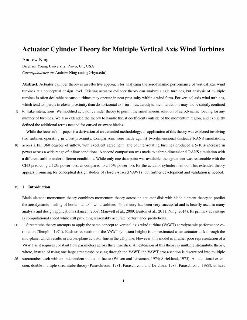
two actuator disks to represent the upstream and downstream sides of the cylinder (Fig. 1). In this model momentum losses

can occur on both the upwind and downwind faces. Double multiple streamtube theory has been widely used for aerodynamic

analysis of VAWTs.

V

V

0

V1

Figure 1. Double multiple streamtube concept with multiple streamtubes along the VAWT (one shown) and separate “actuator disks” on both

the upstream and downstream surfaces.

While double multiple streamtube theory is a useful improvement over single streamtube models, it is clearly a forced

application of the actuator disk concept to a VAWT. A more physically consistent theory for VAWTs, called actuator cylinder5

theory, was developed by Madsen (Madsen, 1982; Madsen et al., 2013). Actuator cylinder theory has been shown to be more

accurate than double multiple streamtube theory (Ferreira et al., 2014), while still retaining comparable computational speed.

One limitation of actuator cylinder theory is that it is derived only for a single isolated turbine. We are interested in per-

formance of VAWT farms, and thus need to predict performance of multiple VAWTs in proximity to each other. This paper

extends the methodology for use with any number of VAWTs, extends applicability to turbines not operating in the momentum10

region, and adds computation details for blades that are curved or swept. The primary purpose of this paper is to derive the new

methodology, but some example trade studies of VAWT pairs are also discussed.

2 Theory Development

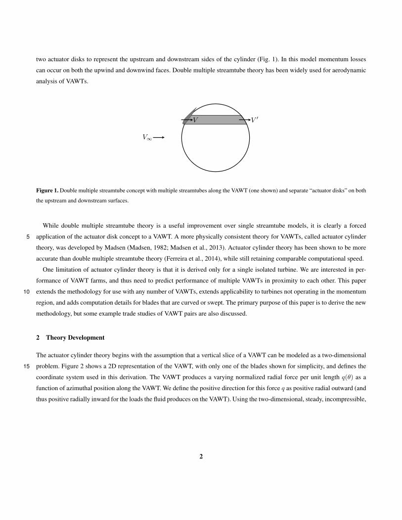
The actuator cylinder theory begins with the assumption that a vertical slice of a VAWT can be modeled as a two-dimensional

problem. Figure 2 shows a 2D representation of the VAWT, with only one of the blades shown for simplicity, and defines the15

coordinate system used in this derivation. The VAWT produces a varying normalized radial force per unit length q(✓) as a

function of azimuthal position along the VAWT. We define the positive direction for this force q as positive radial outward (and

thus positive radially inward for the loads the fluid produces on the VAWT). Using the two-dimensional, steady, incompressible,

2

✓

x

y

V1

q(✓)

Figure 2. A canonical 2D slice of a VAWT (only one blade shown) and the coordinate system used.

Euler equations, and (for the moment) neglecting nonlinear terms, the induced velocities at any location in the plane can be

shown to be given by the following integrals (Madsen et al., 2013; Madsen, 1982):

u(x,y) =

1

2⇡

2⇡Z

0

q(✓)

[x + sin✓] sin✓ � [y � cos✓] cos✓

[x + sin✓]

2+ [y � cos✓]

2d✓

� q(cos

�1y) {inside and wake}

+ q(�cos

�1y) {wake only}

v(x,y) =

1

2⇡

2⇡Z

0

q(✓)

[x + sin✓] cos✓ + [y � cos✓] sin✓

[x + sin✓]

2+ [y � cos✓]

2d✓

(1)

where the x,y position is measured from the center of a unit radius turbine, and velocities are normalized by the freestream

velocity. For evaluation points inside the cylinder the {inside and wake} term applies, and for evaluation points downstream5

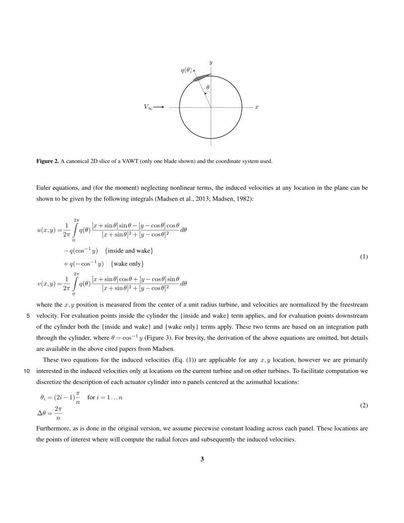
of the cylinder both the {inside and wake} and {wake only} terms apply. These two terms are based on an integration path

through the cylinder, where ✓ = cos

�1y (Figure 3). For brevity, the derivation of the above equations are omitted, but details

are available in the above cited papers from Madsen.

These two equations for the induced velocities (Eq. (1)) are applicable for any x,y location, however we are primarily

interested in the induced velocities only at locations on the current turbine and on other turbines. To facilitate computation we10

discretize the description of each actuator cylinder into n panels centered at the azimuthal locations:

✓

i

= (2i � 1)

⇡

n

for i = 1 . . .n

�✓ =

2⇡

n

(2)

Furthermore, as is done in the original version, we assume piecewise constant loading across each panel. These locations are

the points of interest where will compute the radial forces and subsequently the induced velocities.

3

✓

y

integration path

Figure 3. Integration path for a point inside the cylinder.

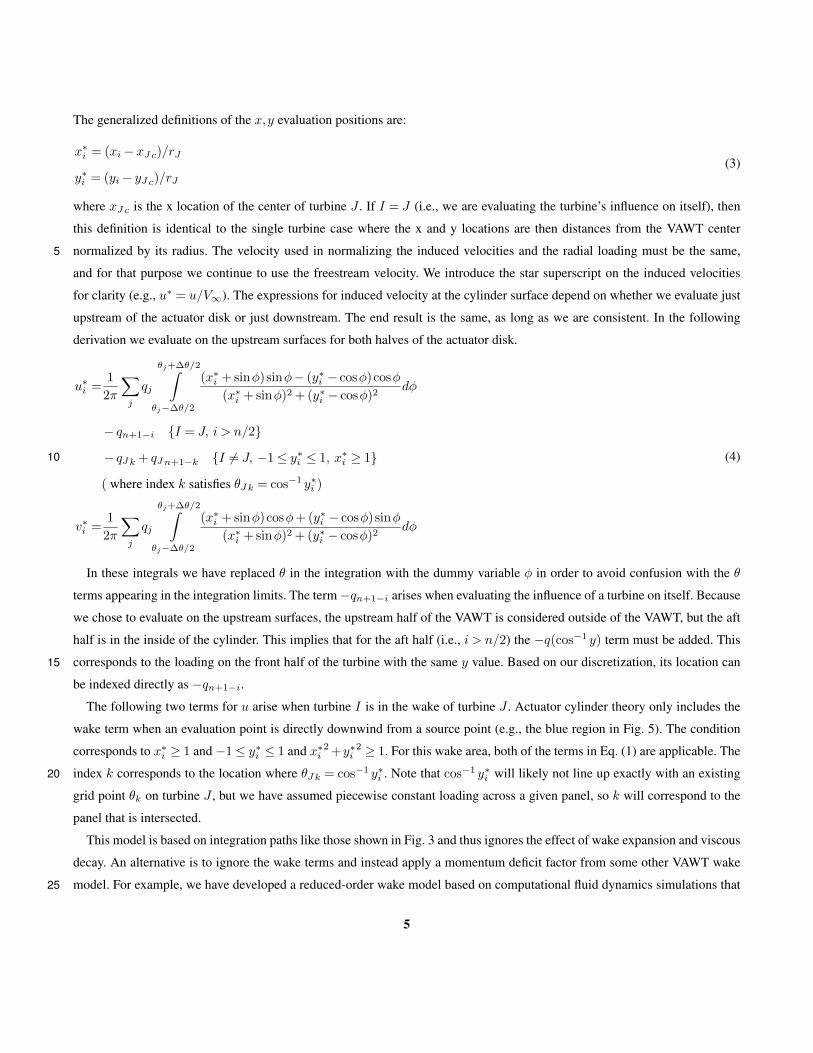
In general, we need to compute the induced velocity at every location on a given VAWT using contributions from all VAWTs

(including itself). In the following derivation we adopt the notation that index I is the turbine we are evaluating the velocities at,

and index i represents the azimuthal location on turbine I where we are evaluating. Index J will refer to the turbine producing

the induced velocity, and index j will indicate the azimuthal location on turbine J where the load is producing the induced

velocity (Fig. 4).5

I

J

i

j

u

i

v

i

q

j

✓

j

Figure 4. Influence of load at location j of turbine J onto location i of turbine I

Using the azimuthal discretization, the induced velocities at a point (x,y) are expressed as a sum of integrals over individual

panels. Recall that Eq. (1) is normalized based on the current VAWT radius and the freestream velocity. Because we are now

considering multiple VAWTs with potentially different radii, we need to be more explicit in defining the normalized quantities.

4

The generalized definitions of the x,y evaluation positions are:

x

⇤i

= (x

i

� x

J

c

)/r

J

y

⇤i

= (y

i

� y

J

c

)/r

J

(3)

where x

J

c

is the x location of the center of turbine J . If I = J (i.e., we are evaluating the turbine’s influence on itself), then

this definition is identical to the single turbine case where the x and y locations are then distances from the VAWT center

normalized by its radius. The velocity used in normalizing the induced velocities and the radial loading must be the same,5

and for that purpose we continue to use the freestream velocity. We introduce the star superscript on the induced velocities

for clarity (e.g., u

⇤= u/V1). The expressions for induced velocity at the cylinder surface depend on whether we evaluate just

upstream of the actuator disk or just downstream. The end result is the same, as long as we are consistent. In the following

derivation we evaluate on the upstream surfaces for both halves of the actuator disk.

u

⇤i

=

1

2⇡

X

j

q

j

✓j+�✓/2Z

✓j��✓/2

(x

⇤i

+ sin�)sin� � (y

⇤i

� cos�)cos�

(x

⇤i

+ sin�)

2+ (y

⇤i

� cos�)

2d�

� q

n+1�i

{I = J, i > n/2}

� q

J

k

+ q

J

n+1�k

{I 6= J, �1 y

⇤i

1, x

⇤i

� 1}

( where index k satisfies ✓

J

k

= cos

�1y

⇤i

)

v

⇤i

=

1

2⇡

X

j

q

j

✓j+�✓/2Z

✓j��✓/2

(x

⇤i

+ sin�)cos� + (y

⇤i

� cos�)sin�

(x

⇤i

+ sin�)

2+ (y

⇤i

� cos�)

2d�

(4)10

In these integrals we have replaced ✓ in the integration with the dummy variable � in order to avoid confusion with the ✓

terms appearing in the integration limits. The term �q

n+1�i

arises when evaluating the influence of a turbine on itself. Because

we chose to evaluate on the upstream surfaces, the upstream half of the VAWT is considered outside of the VAWT, but the aft

half is in the inside of the cylinder. This implies that for the aft half (i.e., i > n/2) the �q(cos

�1y) term must be added. This

corresponds to the loading on the front half of the turbine with the same y value. Based on our discretization, its location can15

be indexed directly as �q

n+1�i

.

The following two terms for u arise when turbine I is in the wake of turbine J . Actuator cylinder theory only includes the

wake term when an evaluation point is directly downwind from a source point (e.g., the blue region in Fig. 5). The condition

corresponds to x

⇤i

� 1 and �1 y

⇤i

1 and x

⇤i

2+y

⇤i

2 � 1. For this wake area, both of the terms in Eq. (1) are applicable. The

index k corresponds to the location where ✓

J

k

= cos

�1y

⇤i

. Note that cos

�1y

⇤i

will likely not line up exactly with an existing20

grid point ✓

k

on turbine J , but we have assumed piecewise constant loading across a given panel, so k will correspond to the

panel that is intersected.

This model is based on integration paths like those shown in Fig. 3 and thus ignores the effect of wake expansion and viscous

decay. An alternative is to ignore the wake terms and instead apply a momentum deficit factor from some other VAWT wake

model. For example, we have developed a reduced-order wake model based on computational fluid dynamics simulations that25

5

predicts the velocity deficit behind a VAWT (Tingey and Ning, 2016). Rather than use the above wake terms, one could use the

separate wake model to evaluate the velocity deficit at each control point and subtract the deficit from u

⇤. Because the focus

on this paper is on actuator cylinder theory we will use the simple wake model that naturally arises within the theory itself, but

this methodology provides a convenient hook to insert any wake model.

J

Figure 5. Wake region from actuator cylinder theory highlighted in blue (and extending downstream).

For convenience in the computation, Eq. (4) can be expressed as a matrix vector multiplication where the loading q is5

separated from the influence coefficients.

u

⇤I

= A

x

IJ

q

J

v

⇤I

= A

y

IJ

q

J

(5)

The matrix A

y

IJ

is given by:

A

y

IJ

(i, j) =

1

2⇡

✓j+�✓/2Z

✓j��✓/2

(x

⇤i

+ sin�)cos� + (y

⇤i

� cos�)sin�

(x

⇤i

+ sin�)

2+ (y

⇤i

� cos�)

2d� (6)

For the A

x

IJ

matrix we divide the contributions between the direct influence and the wake influence: A

x

IJ

= D

x

IJ

+ W

x

IJ

10

where

D

x

IJ

(i, j) =

1

2⇡

✓j+�✓/2Z

✓j��✓/2

(x

⇤i

+ sin�)sin� � (y

⇤i

� cos�)cos�

(x

⇤i

+ sin�)

2+ (y

⇤i

� cos�)

2d� (7)

W

x

IJ

(i, j) =

8>>>>>>>>>><

>>>>>>>>>>:

�1 if � 1 y

⇤i

1 and x

⇤i

� 0

and x

⇤i

2+ y

⇤i

2 � 1 and j = k

1 if � 1 y

⇤i

1 and x

⇤i

� 0

and x

⇤i

2+ y

⇤i

2 � 1 and j = n � k + 1

0 otherwise

(8)

where index k corresponds to the panel where ✓

J

k

= cos

�1y

⇤i

.15

If we are evaluating the influence of a turbine on itself (e.g., I = J) then the computations in the A

x

matrix can be simplified.

We can expand using the definitions for x and y along the cylinder (x⇤i

= �sin✓

i

and y

⇤i

= cos✓

i

for i = 1 . . .n). As long as

6

i 6= j, then the integral in Eq. (7) evaluates to �✓/2. When i = j the value of the integral depends on which side of the cylinder

we evaluate on. It converges to ⇡(�1 + 1/n) just outside of the cylinder and ⇡(1 + 1/n) just inside. Because we chose to

evaluate on the upstream surface on both halves of the cylinder then the integral evaluates to ⇡(�1+1/n) on the upstream half

of the cylinder and ⇡(1 + 1/n) on the downstream half of the cylinder.

D

x

II

(i, j) =

8>>>><

>>>>:

�✓/(4⇡) if i 6= j

(�1 + 1/n)/2 if i = j and i n/2

(1 + 1/n)/2 if i = j and i > n/2

(9)5

W

x

II

(i, j) =

8><

>:

�1 if i > n/2 and j = n + 1� i

0 otherwise(10)

If a user elects to use a more sophisticated wake model the W

x

term can simply be ignored and a separate momentum deficit

factor can be applied.

2.1 Faster Computation10

The bulk of the computational effort is contained in computing the influence coefficient matrices A

x

IJ

and A

y

IJ

. These

computations consist of a double loop iterating across all evaluation positions i on turbine I for each source position j on

turbine J (which is itself contained in a double loop across all turbines I and J). Fortunately, some of this computation can

be simplified. The expressions in Eqs. (6), (9) and (10) apply for the cases where I = J , or in other words for computing the

influence of the turbine on itself. A significant benefit to this equation form, is that the matrices depend only on the discretization15

of the cylinder, and not on the details of the blade shape or loading. For a preselected number of azimuthal segments (e.g.,

n = 36), these matrices can be precomputed and stored. This is true no matter what size radius the VAWT is.

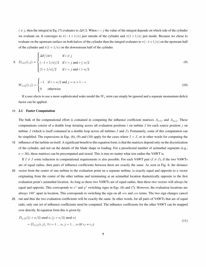
If I 6= J some reduction in computational requirements is also possible. For each VAWT pair (I 6= J), if the two VAWTs

are of equal radius, then pairs of influence coefficients between them are exactly the same. As seen in Fig. 6, the distance

vector from the center of one turbine to the evaluation point on a separate turbine, is exactly equal and opposite to a vector20

originating from the center of the other turbine and terminating at an azimuthal location diametrically opposite to the first

evaluation point’s azimuthal location. As long as these two VAWTs are of equal radius, then these two vectors will always be

equal and opposite. This corresponds to x

⇤ and y

⇤ switching signs in Eqs. (6) and (7). However, the evaluation locations are

always 180

� apart in location. This corresponds to switching the sign on all sin and cos terms. The two sign changes cancel

out and thus the two evaluation coefficients will be exactly the same. In other words, for all pairs of VAWTs that are of equal25

radii, only one set of influence coefficients need be computed. The influence coefficients for the other VAWT can be mapped

over directly. In equation form this is given by

D

x

JI

((i + n/2) mod n,(j + n/2) mod n)

= D

x

IJ

(i, j), 8 i = 1 . . .n, j = 1 . . .n (if r

I

= r

J

)(11)

7

and similarly for A

y

. Note that there is no symmetry in the wake terms (Eq. (8)). If a second turbine is in the wake of the first,

the first turbine will clearly not be in the wake of the second turbine.

✓

⇡ + ✓

Figure 6. The influence coefficient calculations between a pair of VAWTs will always have paired locations that have exactly equal and

opposite distance vectors if the two VAWTs are of equal radius. These two evaluation locations result in the exact same influence coefficients,

reducing the amount of calculations that must be performed.

Finally, we can reduce the number of computations required for VAWTs that have large separation distances. If a VAWT

pair has a large separation distance (e.g.,p

(x

I

c

� x

J

c

)

2+ (y

I

c

� y

J

c

)

2> 10r

I

), then when iterating across index i the value

for positions x

i

and y

i

will change very little. The computation can be simplified by neglecting these very minor changes and5

instead use the distance between VAWT centers (independent of i):

x

⇤i

! (x

I

c

� x

J

c

)/r

J

y

⇤i

! (y

I

c

� y

J

c

)/r

J

(12)

With this simplification the matrices in Eqs. (6) and (7) can be computing by iterating only in j and filling an entire column per

iteration. Additionally, for these large separations the wake terms should be negligible and can be skipped in the computation.

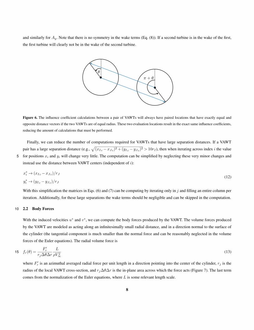
2.2 Body Forces10

With the induced velocities u

⇤ and v

⇤, we can compute the body forces produced by the VAWT. The volume forces produced

by the VAWT are modeled as acting along an infinitesimally small radial distance, and in a direction normal to the surface of

the cylinder (the tangential component is much smaller than the normal force and can be reasonably neglected in the volume

forces of the Euler equations). The radial volume force is

f

r

(✓) =

F

0r

r

j

�✓�r

L

⇢V

21

(13)15

where F

0r

is an azimuthal averaged radial force per unit length in a direction pointing into the center of the cylinder, r

j

is the

radius of the local VAWT cross-section, and r

j

�✓�r is the in-plane area across which the force acts (Figure 7). The last term

comes from the normalization of the Euler equations, where L is some relevant length scale.

8

x

y

✓

j

�

r

r

j

r

j

�

✓

Figure 7. In-plane area for volume force at a given azimuthal station.

Because the force acts across an infinitesimal small radial distance, the radial force acts as a pressure jump

q(✓) = lim

✏!0

1

L

rj+✏Z

rj�✏

f

r

(✓)dr

= lim

✏!0

1

L

rj+✏Z

rj�✏

F

0r

r

j

�✓dr

L

⇢V

21

dr

=

F

0r

r

j

�✓

1

⇢V

21

(14)

the 1/L is necessary to be consistent with the normalization. It does not matter which reference length is used in normalizing

q(✓) because the length scales cancel.

Figure 8 shows the relative components of velocity in the frame of the airfoil. It consists of contributions from the freestream5

velocity, the velocity due to rotation, and the induced velocities from itself and other turbines.

Vj

= V1(1 + u

j

)x + V1v

j

y � ⌦

j

r

j

ˆ

t (15)

Using the following coordinate transformations

x = �cos✓

j

ˆ

t � sin✓

j

n

y = �sin✓

j

ˆ

t + cos✓

j

n

(16)

the velocity can be expressed in the n � ˆ

t plane as10

Vj

=[�V1(1 + u

j

)sin✓

j

+ V1v

j

cos✓

j

] n

+[�V1(1 + u

j

)cos✓

j

� V1v

j

sin✓

j

� ⌦

j

r

j

]

ˆ

t

(17)

9

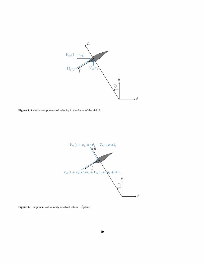
n

ˆ

t

x

y

V1(1 + u

j

)

V1v

j

✓

j

⌦

j

r

j

Figure 8. Relative components of velocity in the frame of the airfoil.

n

ˆ

t

x

y

✓

j

V1(1 + u

j

) sin ✓

j

� V1v

j

cos ✓

j

V1(1 + u

j

) cos ✓

j

+ V1v

j

sin ✓

j

+ ⌦

j

r

j

Figure 9. Components of velocity resolved into n� t plane.

10

These velocity components are depicted in Figure 9.

If we define the magnitudes

V

n

j

⌘ V1(1 + u

j

)sin✓ � V1v

j

cos✓

V

t

j

⌘ V1(1 + u

j

)cos✓ + V1v

j

sin✓ + ⌦

j

r

j

(18)

then

Vj

= �V

n

j

n � V

t

j

ˆ

t (19)5

and the magnitude of the local relative velocity and local inflow angle (Fig. 10) are

W

j

=

qV

n

2j

+ V

t

2j

�

j

= tan

�1

✓V

n

j

V

t

j

◆ (20)

The angle of attack, Reynolds number, and lift and drag coefficients can then be estimated as

↵

j

= �

j

� �

Re

j

=

⇢W

j

c

µ

c

l

j

= f(↵

j

,Re

j

)

c

d

j

= f(↵

j

,Re

j

)

(21)

This can be rotated into normal and tangential force coefficients (note that c

n

is defined as positive in the opposite direction of10

n in Figure 10).

c

n

j

= c

l

j

cos�

j

+ c

d

j

sin�

j

c

t

j

= c

l

j

sin�

j

� c

d

j

cos�

j

(22)

We can resolve these normal and tangential loads into a radial, tangential, and vertical coordinate system. In doing so, we

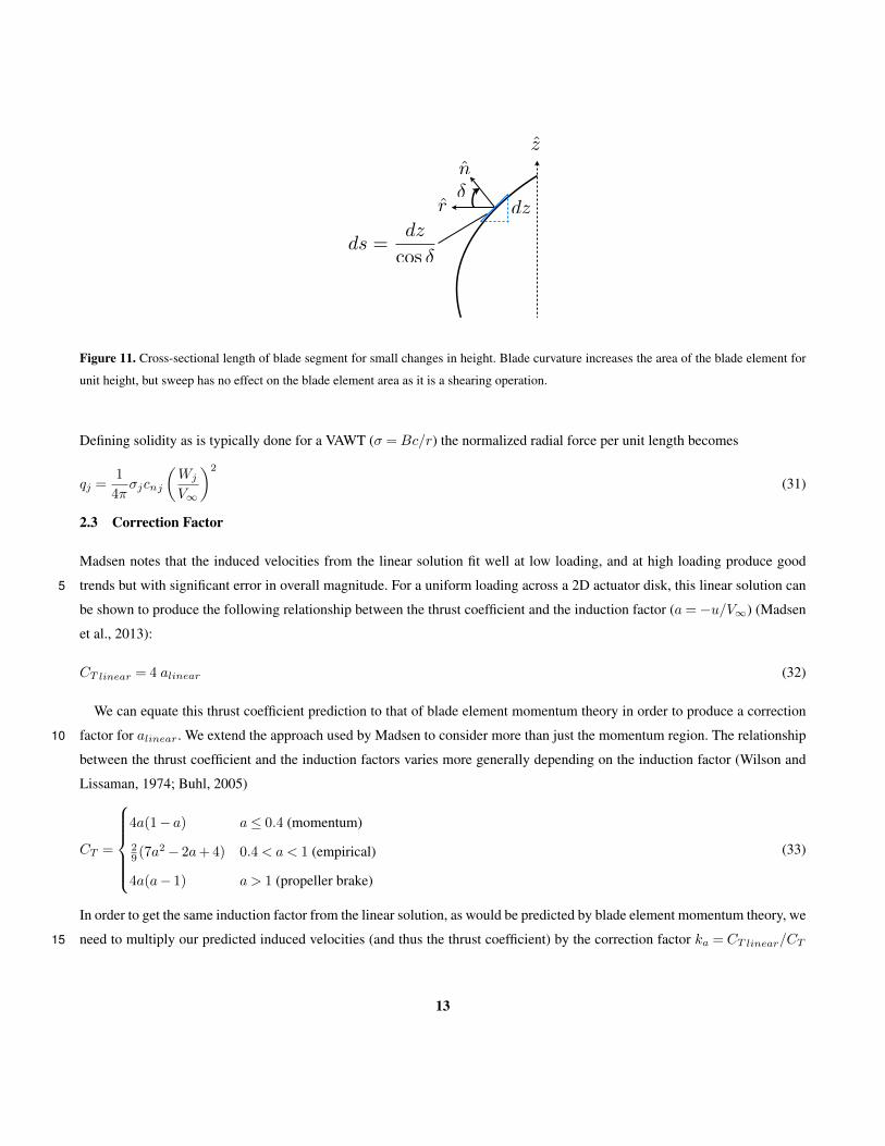
will account for blade curvature, as is often used with VAWTs, an example of which is shown in Fig. 11. The total force vector

is resolved as15

F =

1

2

⇢W

2(�c

n

n + c

t

ˆ

t)�a (23)

where the negative sign results from the coordinate system definition seen in Fig. 10. From Fig. 11 we see that the area of the

blade element is

�a = c �s = c

�z

cos�

(24)

and the unit vector n can be expressed as20

n = cos�r + sin�z (25)

11

W

�

ˆ

t

n

c

n

c

t

c

l

c

d

Figure 10. Definition of normal and tangential force coefficients.

Thus, the force vector per unit depth (unit length in the z-direction) is

F

0=

⇢W

2c

2cos�

(�c

n

cos� r � c

n

sin� z + c

t

ˆ

t) (26)

We can simplify these expressions for the three instantaneous force components

R

0= �c

n

1

2

⇢W

2c

T

0= c

t

1

2

⇢W

2 c

cos�

Z

0= �c

n

1

2

⇢W

2ctan�

(27)

Note that the radial force is unaffected by blade curvature because although the in-plane normal force varies with the cosine5

of the local curvature angle � (Fig. 11), the area over which the force acts varies inversely with the cosine of the angle. Blade

sweep is also permitted, however it is assumed that the sweep is accomplished through shearing rather than rotation. In other

words, it assumed that the airfoils are still defined relative to the streamwise direction as opposed to normal to the local blade

sweep. Thus, sweeping does not increase the area of the blade element.

For equating with the actuator cylinder theory, only the radial force is of interest (but all components will be of use for10

computing overall power and loads). Because the blades are rotating we need to compute an azimuthally averaged value of the

radial loading (recalling the sign convention for a positive radial loading is inward for loads the fluid produces on the VAWT)

F

0r

j

= c

n

j

1

2

⇢W

2j

c

B�✓

2⇡

(28)

Substituting into Eq. (14) to find that the radial volume force can be expressed as

q

j

= c

n

j

1

2

⇢W

2j

c

B�✓

2⇡

1

r

j

�✓

1

⇢V

21

(29)15

After simplification the radial force is

q

j

=

Bc

4⇡r

j

c

n

j

✓W

j

V1

◆2

(30)

12

n

r

z

�

dz

ds =

dz

cos �

Figure 11. Cross-sectional length of blade segment for small changes in height. Blade curvature increases the area of the blade element for

unit height, but sweep has no effect on the blade element area as it is a shearing operation.

Defining solidity as is typically done for a VAWT (� = Bc/r) the normalized radial force per unit length becomes

q

j

=

1

4⇡

�

j

c

n

j

✓W

j

V1

◆2

(31)

2.3 Correction Factor

Madsen notes that the induced velocities from the linear solution fit well at low loading, and at high loading produce good

trends but with significant error in overall magnitude. For a uniform loading across a 2D actuator disk, this linear solution can5

be shown to produce the following relationship between the thrust coefficient and the induction factor (a = �u/V1) (Madsen

et al., 2013):

C

T

linear

= 4 a

linear

(32)

We can equate this thrust coefficient prediction to that of blade element momentum theory in order to produce a correction

factor for a

linear

. We extend the approach used by Madsen to consider more than just the momentum region. The relationship10

between the thrust coefficient and the induction factors varies more generally depending on the induction factor (Wilson and

Lissaman, 1974; Buhl, 2005)

C

T

=

8>>>><

>>>>:

4a(1 � a) a 0.4 (momentum)

29 (7a

2 � 2a + 4) 0.4 < a < 1 (empirical)

4a(a � 1) a > 1 (propeller brake)

(33)

In order to get the same induction factor from the linear solution, as would be predicted by blade element momentum theory, we

need to multiply our predicted induced velocities (and thus the thrust coefficient) by the correction factor k

a

= C

T

linear

/C

T

15

13

The correction factors become

k

a

=

8>>>><

>>>>:

1/(1 � a) (momentum)

(18a)/(7a

2 � 2a + 4) (empirical)

1/(a � 1) (propeller brake)

(34)

In order to determine the value of a to use in the above equation we first find the thrust coefficient. The instantaneous thrust

coefficient can be found from Eq. (27) using the coordinate system definition that

X

0= �R

0sin✓ � T

0cos✓

=

1

2

⇢W

2c

✓c

n

sin✓ � c

t

cos✓

cos�

◆ (35)5

The instantaneous thrust coefficient is

C

T

inst

=

X

0

12⇢V

21(2r)

=

✓W

V1

◆2c

2r

✓c

n

sin✓ � c

t

cos✓

cos�

◆ (36)

where the other normalization dimension comes from the distributed loads, which are a force per unit length in the z-direction.

To get the total thrust coefficient we need to compute the azimuthal average

C

T

=

B

2⇡

2⇡Z

0

C

T

inst

(✓)d✓

=

�

4⇡

2⇡Z

0

✓W

V1

◆2✓c

n

sin✓ � c

t

cos✓

cos�

◆d✓

(37)10

From the thrust coefficient we can compute the expected induction factor by reversing Eq. (33)

a =

8>>>><

>>>>:

12

�1 �

p1 � C

T

�C

T

0.96 (momentum)

17

⇣1 + 3

q72C

T

� 3

⌘0.96 < C

T

< 2 (empirical)

12

�1 +

p1 + C

T

�C

T

> 2 (propeller brake)

(38)

Finally, this induction factor allows us to compute the correction factor from Eq. (34). These factors should be multiplied

against the induced velocities, but because that is the quantity we need to solve for, we must multiply against their predicted

values.15

Because this correction is derived for an isolated turbine, the correction factors k1 . . .k

N

should be precomputed for each

individual turbine in isolation rather than as part of the coupled solve of all turbines together.

14

2.4 Matrix Assembly and Solution Procedure

From the proceeding discussion it should be noted that computing that loads depends on the induced velocities, but computing

the induced velocities depends on the loads. Thus, an iterative root-finding approach is required. We can assemble the self-

induction and mutual induction effects into one large matrix composed of block matrices. We also need to apply the various

correction factors k for turbine J . To solve all induced velocities as one large system we will concatenate the u and v velocity5

vectors into one vector: w = [u;v]. In the equation below, the symbol � represents an element-by-element multiplication.2

666666666666666666664

u1

u2

...

u

N

��v1

v2

...

v

N

3

777777777777777777775

=

2

666666666666666666664

k1

k2

...

k

N

��k1

k2

...

k

N

3

777777777777777777775

�

2

666666666666666666664

A

x

A

x12 . . . A

x1N

A

x21 A

x

. . . A

x2N

......

. . ....

A

x

N1 A

x

N2 . . . A

x

� � � � � � � � � � �� � � � � �A

y

A

y12 . . . A

y1N

A

y21 A

y

. . . A

y2N

......

......

A

y

N1 A

y

N2 . . . A

y

3

777777777777777777775

2

666664

q1

q2

...

q

N

3

777775(39)

We now have a matrix vector expression of the form: w = Aq, but because q depends on w we must solve for w using a root

finding method. The residual equation is:

f(w) = Aq(w) � w = 0 (40)10

Any good n-dimensional root finder can be used. This paper uses the modified Powell Hybrid method as contained in hybrd.f

of minpack.

2.5 Variations in Height

The actuator cylinder theory computes all loads in 2-dimensional cross-sections. We can either use a representative section to

represent the whole turbine (which is more appropriate for an H-Darrieus geometry, ignoring wind shear), or we can addition-15

ally discretize the turbine along the height and compute loads at each section.

For each azimuthal station of interest, the solution is projected onto the instantaneous locations of the blade discretization as

shown in Fig. 12. For an unswept blade, this involves just a straightforward transfer of forces as the blade discretization would

typically be exactly aligned with the surface discretization. However, for swept blades, interpolation is necessary to resolve

the forces along the curved blade path. Furthermore, for a swept blade, the normal and tangential directions change along the20

blade path. For swept blades, each point along the blade is at some azimuthal offset (�✓) from a reference point (e.g., relative

to the the equatorial blade location), and the total normal force, tangential force, and torque produced by the blade are (again

15

Figure 12. Example two-dimensional discretization in height and azimuthal position of swept surface (side-view).

�✓ = 0 for unswept blades)

R

blade

(✓) =

Z[R

0(✓ + �✓)cos(�✓)

� T

0(✓ + �✓)sin(�✓)]dz

T

blade

(✓) =

Z[R

0(✓ + �✓)sin(�✓)

+ T

0(✓ + �✓)cos(�✓)]dz

Z

blade

(✓) =

ZZ

0(✓ + �✓)dz

Q

blade

(✓) =

ZrT

0(✓ + �✓)dz

(41)

Now that the forces as a function of ✓ are known for one blade, the forces for all B blades can be found. We let �⇥

j

represent the offset of blade j relative to the first blade

�⇥

j

= 2⇡(j � 1)/B (42)5

The resulting forces in the inertial frame are then

X

all�blades

(✓) =

BX

j=1

�R

blade

(✓ + �⇥

j

)sin(✓ + �⇥

j

)

� T

blade

(✓ + �⇥

j

)cos(✓ + �⇥

j

)

Y

all�blades

(✓) =

BX

j=1

R

blade

(✓ + �⇥

j

)cos(✓ + �⇥

j

)

� T

blade

(✓ + �⇥

j

)sin(✓ + �⇥

j

)

Z

all�blades

(✓) =

BX

j=1

Z

blade

(✓ + �⇥

j

)

(43)

In this representation the velocities at each height can be different to account for wind shear or other wind distributions.

This derivation is provided for completeness, but because of the increased computational expense, and to be consistent with

the other comparisons we are making in this paper, we will focus on using one 2D slice for the entire turbine.10

16

2.6 Power

In addition to the thrust coefficient and instantaneous loads, which have already been defined, we are also interested in com-

puting the power coefficient. This is easily computed from the instantaneous tangential load given in Eq. (27) (or Eq. (43)).

The torque (per unit length) is then

Q = rT

0 (44)5

and the azimuthally-averaged power is

P =

⌦B

2⇡

2⇡Z

0

Q(✓)d✓ (45)

This is a periodic integral and care should be taken in integrating near the boundaries because of the way the discretization is

defined (✓1 does not start at 0). The power coefficient per unit length is then

C

P

=

P

12⇢V

31(2r)

(46)10

2.7 Clockwise Rotation

The following derivation assumed counterclockwise rotation. For clockwise rotation a few minor changes must be made.

Nothing in the influence coefficients needs changing as those are purely based on location. The only change for clockwise

rotation is that the direction of ˆ

t is reversed, as is the direction of the ⌦r velocity vector in Figs. 8 and 9. The consequence is

that the tangential velocity in Eq. (18) must be redefined as (note the two minus signs)15

V

t

j

⌘ �V1(1 + u

j

)cos✓ � V1v

j

sin✓ + ⌦

j

r

j

(47)

Additionally, the change in tangential direction affects the computation of the thrust coefficient. In Eq. (35) the sign is

reversed on the second part of the equation. The consequence is that the total thrust coefficient (Eq. (37)) would be computed

as

C

T

=

�

4⇡

2⇡Z

0

✓W

V1

◆2✓c

n

sin✓ + c

t

cos✓

cos�

◆d✓ (48)20

For transferring loads to an inertial frame, or for computing total blade loads with curved blades, a couple more changes are

required. Equation (43) replaces the + sign in front of T

blade

with a � sign (for both the X and Y equation) and Eq. (41) is

modified as:

R

blade

(✓) =

Z[R

0(✓ + �✓)cos(�✓)

+ T

0(✓ + �✓)sin(�✓)]dz

T

blade

(✓) =

Z[�R

0(✓ + �✓)sin(�✓)

+ T

0(✓ + �✓)cos(�✓)]dz

(49)

17

3 Two Turbine Interactions

This methodology was implemented and made open-source1 in Julia, which is a dynamic programming language designed for

scientific computing2. For single turbine cases the implementation was verified against Madsen’s results (Madsen et al., 2013).

Our focus here is on multiple turbine cases, and for simplicity on two turbine cases.

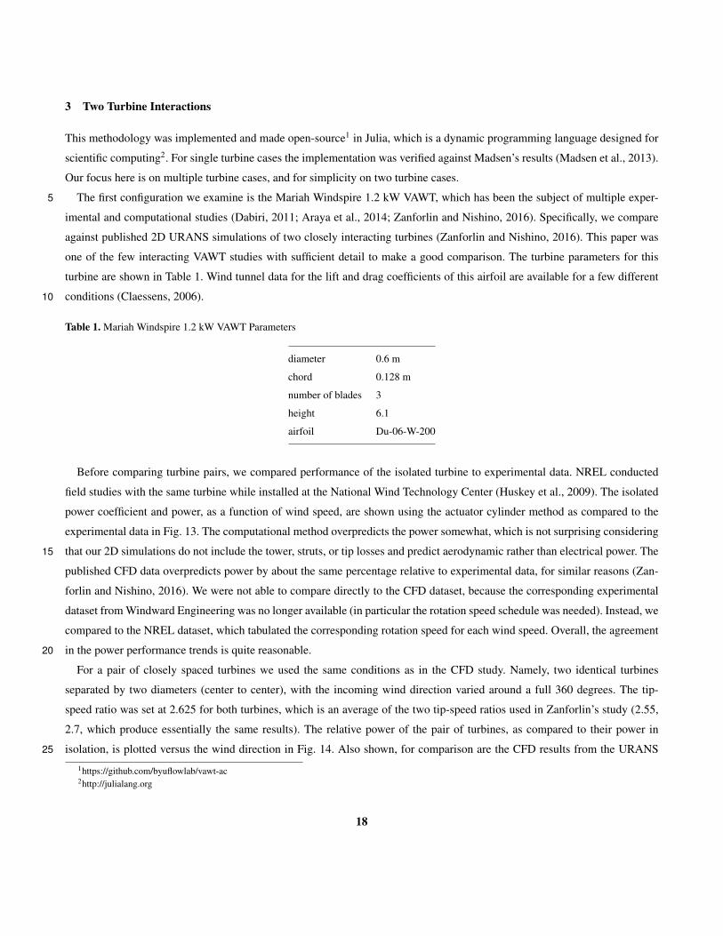
The first configuration we examine is the Mariah Windspire 1.2 kW VAWT, which has been the subject of multiple exper-5

imental and computational studies (Dabiri, 2011; Araya et al., 2014; Zanforlin and Nishino, 2016). Specifically, we compare

against published 2D URANS simulations of two closely interacting turbines (Zanforlin and Nishino, 2016). This paper was

one of the few interacting VAWT studies with sufficient detail to make a good comparison. The turbine parameters for this

turbine are shown in Table 1. Wind tunnel data for the lift and drag coefficients of this airfoil are available for a few different

conditions (Claessens, 2006).10

Table 1. Mariah Windspire 1.2 kW VAWT Parameters

diameter 0.6 m

chord 0.128 m

number of blades 3

height 6.1

airfoil Du-06-W-200

Before comparing turbine pairs, we compared performance of the isolated turbine to experimental data. NREL conducted

field studies with the same turbine while installed at the National Wind Technology Center (Huskey et al., 2009). The isolated

power coefficient and power, as a function of wind speed, are shown using the actuator cylinder method as compared to the

experimental data in Fig. 13. The computational method overpredicts the power somewhat, which is not surprising considering

that our 2D simulations do not include the tower, struts, or tip losses and predict aerodynamic rather than electrical power. The15

published CFD data overpredicts power by about the same percentage relative to experimental data, for similar reasons (Zan-

forlin and Nishino, 2016). We were not able to compare directly to the CFD dataset, because the corresponding experimental

dataset from Windward Engineering was no longer available (in particular the rotation speed schedule was needed). Instead, we

compared to the NREL dataset, which tabulated the corresponding rotation speed for each wind speed. Overall, the agreement

in the power performance trends is quite reasonable.20

For a pair of closely spaced turbines we used the same conditions as in the CFD study. Namely, two identical turbines

separated by two diameters (center to center), with the incoming wind direction varied around a full 360 degrees. The tip-

speed ratio was set at 2.625 for both turbines, which is an average of the two tip-speed ratios used in Zanforlin’s study (2.55,

2.7, which produce essentially the same results). The relative power of the pair of turbines, as compared to their power in

isolation, is plotted versus the wind direction in Fig. 14. Also shown, for comparison are the CFD results from the URANS25

1https://github.com/byuflowlab/vawt-ac2http://julialang.org

18

Figure 13. Power and power coefficient (separate y axes), as a function of wind speed for the Windspire 1.2 kW Turbine. Lines are from the

actuator cylinder method (AC), and circles are from the NREL experimental data.

study (Zanforlin and Nishino, 2016). While small differences exist, the overall agreement is very good. Benefits on the order

of 5–10% are observed across a relatively wide range on inflow angles. These results are also in alignment with those observed

experimentally for this same turbine (Dabiri, 2011).

Figure 14. Normalized power as a function of wind direction on a polar plot, with an overlay of the turbine rotation directions. Results shown

for both the actuator cylinder method (AC), and for the CFD results of (Zanforlin and Nishino, 2016).

Repeating this exercise for many different separations (e.g., two diameters was used in the previous case), requires a different

visualization approach, otherwise the plots overlap and become difficult to see. Instead of changing the wind direction for a5

fixed turbine position, we move the turbines around for a fixed wind position. The position of turbine 1 is fixed, and the position

19

of turbine 2 is swept in concentric circles ranging from 1 diameters (no separation) to 6 diameters between turbine centers. The

lower bound is of course unrealistically close, but because some VAWT concepts employ dual rotors with very close spacings,

the smallest possible lower bound was used to observe trends across a broader range. By moving the turbines we can show the

effect of relative separation and changing wind direction (via rotated positions) simultaneously.

Figure 15 shows the normalized power (total power of the turbines relative to their total power in isolation) as a function of5

the position of turbine 2 for counter-rotating turbines. Overlays of turbine 1 (fixed) and turbine 2 (position changed) are shown

on the plots. The blank regions upstream and downstream of turbine 1 are regions where one of the turbines is in the other’s

wake. In these cases, the power drops by a large amount, well below the range of the color bars. The colorbar range was chosen

to highlight the mutual interference outside of the wake, which is of greater interest. We observe large regions of beneficial

interference of around 5–10% for closely spaced turbines (with benefits exceeding 10% for very close spacings).10

Figure 15. The first turbine is fixed in the center, and the second turbine is moved around in concentric circles with the wind incoming from

the left. The contours show the normalized power of the two turbines (sum of their power normalized by sum of their power in isolation). The

color scale is centered on 1.0 so that regions of beneficial interference can be more clearly seen. The color scale focuses on a small region

(0.9–1.1) for the same reason. The blank areas are waked regions, in which the power drops below the range of the color scale and so are not

plotted.

For counter rotating turbines, two configurations are possible: the Counter Up and the Counter Down configuration (Fig. 16).

In Fig. 15 the upper half of the figure corresponds to the Counter Up configuration, and the lower half corresponds to the

Counter Down configuration. For the current turbine and conditions, the Counter Down configuration shows somewhat larger

benefits across a wider range of inflow angles, consistent with the reported CFD studies. A co-rotating configuration was also

explored, which yielded very similar regions of beneficial interference. The figures were so similar in these conditions, that a15

separate plot for the co-rotating case is not shown.

20

V1 V1

Counter Up Counter Down

Figure 16. Two cases for a counter rotating pair of turbines. “Counter Up” refers to the pair with a rotation direction facing upstream at their

closest interface, where as the “Counter Down” configuration rotates downstream at their closest interface.

A second turbine and condition set came from a three-dimensional incompressible Navier-Stokes simulation (Korobenko

et al., 2013). This turbine was a 3.5 kW H-Darrieus from Cleanfield Energy Corporation. The turbine parameters are listed in

Table 2. Wind tunnel data for the airfoil was extracted from Sandia wind tunnel tests (Sheldahl and Klimas, 1981). The lift

and drag coefficients change significantly at the Reynolds number of this turbine (275,000), and so to provide the best estimate

possible the coefficient data was interpolated between the two nearest datasets: Re = 160,000 and Re = 360,000.5

Table 2. Cleanfield 3.5 kW VAWT Parameters

diameter 2.5 m

chord 0.4 m

number of blades 3

height 3

airfoil NACA 0015

Because three-dimensional CFD is more computationally intensive, only one case was included in that study to compare

against. That case consisted of two turbines in the Counter Down configuration, separated (tower to tower) by 2.64 rotor radii.

The turbines were operated at a tip-speed ratio of 1.5, which was the optimal condition for the single turbine configuration.

The CFD study reported a decrease in power for the counter-rotating pair, although the amount of decrease was not specified.

Fortunately, torque vs. azimuth plots were presented. Extracting that data from the plot and integrating, shows that the CFD10

simulations predicted a 12% decrease in power for the counter-rotating pair as compared to the isolated turbines.

Actuator cylinder theory was used for the same turbine at the optimal tip-speed ratio predicted using AC theory. A decrease

in power for the Counter Down configuration was also observed of about 15%. However, the optimal tip-speed ratio differed

from the experimental data (Bravo et al., 2007). The nondimensional power curves were very similar, but with a shift in tip-

speed ratio. To be consistent, the optimal tip-speed ratio was used in both cases (2.9 for the actuator cylinder case). Without15

more data to compare against, the robustness of this configuration to other conditions could not be assessed.

21

A third dataset was examined, this from wind tunnel tests of co- and counter- rotating VAWTs pairs (Ahmadi-Baloutaki

et al., 2015). This study used very high solidity rotors and found beneficial interference for counter-rotating turbines across

all wind speeds tested. For co-rotating turbines beneficial interference was realized across some wind speeds, and detrimental

interference at others. The turbines used in this wind tunnel study were inefficient under the conditions tested, with an extremely

small power coefficient of 2⇥10

�3 (corresponding power of under 0.3 W). The percent increase in power of turbine pairs was5

significant, but in absolute terms the power increase was very small. Similar relative benefits with actuator cylinder theory were

observed depending on the assumed airfoil data. This turbine used a custom-made airfoil section and, without corresponding

wind tunnel data, detailed comparisons to actuator cylinder theory was not possible.

In addition to comparing power output, we compared the induced velocity field generated by the VAWT. Ultimately, this

induced velocity is what changes the incoming flow field for a second turbine. The streamlines for the induced velocity field of10

the isolated VAWT and the total velocity field (with freestream added) are shown in Fig. 17. For comparison, the streamlines

for a solution based on the full Euler equations is shown below (Madsen, 1982). Although the actuator cylinder theory uses a

linearization, and only adds a nonlinear correction, the induced and total velocity fields compare well to those from the Euler

equations. These induced velocities were also found to compare well to that from an unsteady panel simulation of a VAWT

(see Figs. 3.7 and 3.8 in (Ferreira, 2009)).15

A properly positioned pair of VAWTs can produce power increases, but one must be careful in extrapolating results to the

wind farm. Even, in just the two turbine case, overall benefits may or may not be realized depending on the site conditions.

Although power increases of around 5–10% may be realized across a wide range of inflow angles, for inflow angles that create

wake interference the power loss can drop by 50%. As an example, assuming a uniform wind rose (wind equally probable in

all directions), the data in Fig. 14 yields an expected value of power of around 90% of that in isolation (both using this method20

and the CFD results). In other words, with a uniform wind rose the wake losses overwhelm the benefits of close spacing. A

more directional wind rose, on the other hand, could realize overall power increases.

Additionally, a wind farm consists of many turbines, and accounting for wake effects across the full wind rose is essential.

VAWTs tend to produce shorter wakes then HAWTs which can help alleviate some of the spacing challenges. However, if

turbines are intentionally positioned close together to create beneficial interference, then they also have the potential to create25

strong power losses through wake effects.

Beneficial interference may be possible not just for pairs of turbines, but for carefully positioned arrays of turbines, as

demonstrated in 2D unsteady RANS simulations (Bremseth and Duraisamy, 2016). However, the benefits have only been

explored with one wind direction. Our past research in HAWT wind farm optimization suggests that when optimizing turbine

positioning under uncertainty of wind direction, the optimal configurations spread out and are not in aligned rows in order to30

minimize wake interference (Fleming et al., 2016; Gebraad et al., 2016). Further investigation is needed to better understand

how to optimize VAWT farms.

22

Figure 17. Top row is for the linear actuator cylinder theory, showing streamlines for an isolated turbine. The left figure shows the induced

velocity only, while the right figure includes the freestream. The bottom row shows the same conditions, but with the full Euler equations

(Madsen, 1982).

4 Conclusions

Actuator cylinder theory is a fast and often effective analysis method to predict aerodynamic loads and power of vertical axis

wind turbines. In this paper we derive an extension to actuator cylinder theory for multiple interacting turbines. Additional

extensions were provided that apply to both the single turbine and multiple turbine cases: thrust coefficients outside of the

momentum regions, and curved or swept blades.5

Comparisons to published data for VAWT pairs showed reasonable agreement in predicting relative power changes and

induced velocities using actuator cylinder theory. However, more data is needed to better assess the conditions under which the

multiple actuator cylinder theory is effective. Like blade element momentum methods, the accuracy and usefulness of actuator

cylinder theory is highly dependent on providing accurate airfoil coefficient data.

For closely-spaced VAWTs, we observed cases with beneficial interference across a wide range of inflow angles, with10

peak power increases exceeding 10%. In other cases, detrimental interference was observed. The conditions that affect the

interactions depend on many things including: the airfoil aerodynamic performance, the tip-speed ratios, and solidities. Our

23

focus here is to demonstrate the actuator cylinder theory and not to make a thorough investigation of closely-interacting

VAWTs, but more illumination on this topic is needed.

Further improvements to actuator cylinder theory are needed, as are more detailed validation studies. An improved wake

model is necessary because the wakes in actuator cylinder theory are inviscid, do not decay, and do not spread. Our recent

work has developed the first VAWT wake model derived from computational fluid dynamics simulations that is parametrized5

for turbines with different tip-speed ratios and solidities (Tingey and Ning, 2016). Models like this could be combined with

actuator cylinder theory to better predict turbine-wake interactions.

Because of the model’s sensitivity to the airfoil data, further data collection, and improved methods of applying rotational

corrections specific to VAWTs may be needed. Although the method was only demonstrated in 2D, as outlined in the methods

section, extensions to 3D are straightforward using a strip-wise approach, but tip-loss corrections should be added. Addition-10

ally, appropriate methods to accounting for losses through struts and the tower will likely improve aerodynamic performance

estimates.

24

References

Ahmadi-Baloutaki, M., Carriveau, R., and Ting, D. S.-K.: Performance of a vertical axis wind turbine in grid generated turbulence, Sustain-

able Energy Technologies and Assessments, 11, 178–185, doi:10.1016/j.seta.2014.12.007, http://dx.doi.org/10.1016/j.seta.2014.12.007,

2015.

Araya, D. B., Craig, A. E., Kinzel, M., and Dabiri, J. O.: Low-order modeling of wind farm aerodynamics using leaky Rankine bodies, J.5

Renewable Sustainable Energy, 6, 063 118, doi:10.1063/1.4905127, http://dx.doi.org/10.1063/1.4905127, 2014.

Bravo, R., Tullis, S., and Ziada, S.: Performance testing of a small vertical-axis wind turbine, in: Proceedings of the 21st Canadian Congress

of Applied Mechanics (CANCAM07), Toronto, Canada, June, pp. 3–7, 2007.

Bremseth, J. and Duraisamy, K.: Computational analysis of vertical axis wind turbine arrays, Theor. Comput. Fluid Dyn.,

doi:10.1007/s00162-016-0384-y, http://dx.doi.org/10.1007/s00162-016-0384-y, 2016.10

Buhl, M. L.: A New Empirical Relationship between Thrust Coefficient and Induction Factor for the Turbulent Windmill State, Tech. Rep.

NREL/TP-500-36834, National Renewable Energy Laboratory, 2005.

Burton, T., Jenkins, N., Sharpe, D., and Bossanyi, E.: Wind Energy Handbook, Wiley, 2nd edn., 2011.

Claessens, M.: The Design and Testing of Airfoils for Application in Small Vertical Axis Wind Turbines, Master’s thesis, Delft University of

Technology, 2006.15

Dabiri, J. O.: Potential Order-of-Magnitude Enhancement of Wind Farm Power Density Via Counter-Rotating Vertical-Axis Wind Turbine

Arrays, J. Renewable Sustainable Energy, 3, 043 104, doi:10.1063/1.3608170, http://dx.doi.org/10.1063/1.3608170, 2011.

Ferreira, C. S.: The Near Wake of the Vawt, Ph.D. thesis, Delft University of Technology, 2009.

Ferreira, C. S., Madsen, H. A., Barone, M., Roscher, B., Deglaire, P., and Arduin, I.: Comparison of Aerodynamic Models for Vertical

Axis Wind Turbines, J. Phys.: Conf. Ser., 524, 012 125, doi:10.1088/1742-6596/524/1/012125, http://dx.doi.org/10.1088/1742-6596/524/20

1/012125, 2014.

Fleming, P., Ning, A., Gebraad, P., and Dykes, K.: Wind Plant System Engineering through Optimization of Layout and Yaw Control, Wind

Energy, 19, 329–344, doi:10.1002/we.1836, 2016.

Gebraad, P., Thomas, J. J., Ning, A., Fleming, P., and Dykes, K.: Maximization of the Annual Energy Production of Wind Power Plants by

Optimization of Layout and Yaw-Based Wake Control, Wind Energy, doi:10.1002/we.1993, 2016.25

Hansen, M. O. L.: Aerodynamics of Wind Turbines, Earthscan, 2nd edn., 2008.

Huskey, A., Bowen, A., and Jager, D.: Wind Turbine Generator System Power Performance Test Report for the Mariah Windspire 1-kW Wind

Turbine, NREL/TP-500-46192, National Renewable Energy Laboratory, doi:10.2172/969714, http://dx.doi.org/10.2172/969714, 2009.

Korobenko, A., Hsu, M.-C., Akkerman, I., and Bazilevs, Y.: Aerodynamic Simulation of Vertical-Axis Wind Turbines, Journal of Applied

Mechanics, 81, 021 011, doi:10.1115/1.4024415, http://dx.doi.org/10.1115/1.4024415, 2013.30

Madsen, H.: The Actuator Cylinder — a Flow Model for Vertical Axis Wind Turbines, Ph.D. thesis, Aalborg University Centre, 1982.

Madsen, H., Larsen, T., Vita, L., and Paulsen, U.: Implementation of the Actuator Cylinder Flow Model in the HAWC2 Code for Aeroelastic

Simulations on Vertical Axis Wind Turbines, in: 51st AIAA Aerospace Sciences Meeting, AIAA 2013-0913, doi:10.2514/6.2013-913,

2013.

Manwell, J. F., Mcgowan, J. G., and Rogers, A. L.: Wind Energy Explained, Wiley, 2nd edn., 2009.35

Ning, A.: A Simple Solution Method for the Blade Element Momentum Equations with Guaranteed Convergence, Wind Energy, 17, 1327–

1345, doi:10.1002/we.1636, http://dx.doi.org/10.1002/we.1636, 2014.

25

Paraschivoiu, I.: Double Multiple Streamtube Model for Darrieus Wind Turbines, in: 2nd DOE/NASA Wind Turbine Dynamics Workshop,

Cleveland, OH, 1981.

Paraschivoiu, I.: Double-multiple streamtube model for studying vertical-axis wind turbines, Journal of Propulsion and Power, 4, 370–377,

doi:10.2514/3.23076, http://dx.doi.org/10.2514/3.23076, 1988.

Paraschivoiu, I. and Delclaux, F.: Double Multiple Streamtube Model with Recent Improvements (for Predicting Aerodynamic Loads and5

Performance of Darrieus Vertical Axis Wind Turbines), Journal of Energy, 7, 250–255, doi:10.2514/3.48077, 1983.

Sheldahl, R. E. and Klimas, P. C.: Aerodynamic characteristics of seven symmetrical airfoil sections through 180-degree angle of attack

for use in aerodynamic analysis of vertical axis wind turbines, SAND80-2114, doi:10.2172/6548367, http://dx.doi.org/10.2172/6548367,

1981.

Strickland, J.: A performance prediction model for the Darrieus turbine, in: International Symposium on Wind Energy Systems, vol. 1, p. 3,10

1975.

Templin, R.: Aerodynamic performance theory for the NRC vertical-axis wind turbine, LTR-LA-160, National Aeronautical Establishment,

Ottawa, Ontario, Canada, 1974.

Tingey, E. and Ning, A.: Parameterized Vertical-Axis Wind Turbine Wake Model Using CFD Vorticity Data, in: ASME Wind Energy

Symposium, San Diego, CA, doi:10.2514/6.2016-1730, 2016.15

Wilson, R. and Lissaman, P.: Applied Aerodynamics of Wind Power Machines, Tech. rep., Oregon State University, 1974.

Zanforlin, S. and Nishino, T.: Fluid dynamic mechanisms of enhanced power generation by closely spaced vertical axis wind turbines,

Renewable Energy, 99, 1213–1226, doi:10.1016/j.renene.2016.08.015, http://dx.doi.org/10.1016/j.renene.2016.08.015, 2016.

26