Active Suppression of Rotating Stall Inception with...

Hindawi Publishing CorporationInternational Journal of Rotating MachineryVolume 2007, Article ID 56808, 15 pagesdoi:10.1155/2007/56808

Research ArticleActive Suppression of Rotating Stall Inception withDistributed Jet Actuation

Huu Duc Vo

Departement de genie mecanique, Ecole Polytechnique de Montreal, Campus Universite de Montreal,2900 boulevard Edouard-Montpetit, 2500 chemin de Polytechnique, bureau C318.9, Montreal,Quebec, Canada H3T 1J4

Received 19 October 2006; Accepted 5 March 2007

Recommended by Meinhard T. Schobeiri

An analytical and experimental investigation of the effectiveness of full-span distributed jet actuation for active suppression oflong length-scale rotating stall inception is carried out. Detailed modeling and experimental verification highlight the importanteffects of mass addition, discrete injectors, and feedback dynamics, which may be overlooked in preliminary theoretical studies ofactive control with jet injection. A model of the compression system incorporating nonideal injection and feedback dynamics isverified with forced response measurements to predict the right trends in the movement of the critical pole associated with the stallprecursor. Active control experiments with proportional feedback control show that the predicted stall precursors are suppressedto give a 5.5% range extension in compressor flow coefficient. In addition, results suggest that the proposed model could be usedto design a more sophisticated controller to further improve performance while reducing actuator bandwidth requirements.

Copyright © 2007 Huu Duc Vo. This is an open access article distributed under the Creative Commons Attribution License, whichpermits unrestricted use, distribution, and reproduction in any medium, provided the original work is properly cited.

1. INTRODUCTION

Aerodynamic instabilities in axial compressors, in the formsurge and rotating stall, are among the main limiting fac-tors in efficiency improvement of current gas turbine en-gines. Surge is a high-amplitude axisymmetric oscillation ofthe flow across the compressor (and gas turbine). Rotatingstall features the formation of a circumferentially nonuni-form velocity disturbance rotating at a fraction of the rotorspeed, with a large drop in pressure ratio. Surge is often trig-gered by rotating stall. Both are detrimental to the perfor-mance and durability of the compressor. Attempts to avoidthem by setting of an operational safety margin often do so atthe expense of efficiency, by positioning the operating pointfurther from the point of maximum efficiency. A modern so-lution pursued by researchers over the past few years is toactively suppress the aerodynamic instabilities with feedbackcontrol and extend the compressor’s operating range. How-ever, its implementation requires an understanding of theseinstabilities.

There are two well-established routes to rotating stall, re-ferred to as long length-scale or “modal” stall inception andshort length-scale or “spike” stall inception, distinguished bythe type of initial perturbation in pressure/velocity.

First described by Day [1], short length-scale stall incep-tion is characterized by the appearance of a local disturbance(or “spike”) two to three blade pitches in width at the ro-tor tip and whose associated velocity defect is comparableto the mean velocity through the compressor. The spike ro-tates at about 70% of the rotor speed and can grow into afull-span circumferentially two-dimensional stall cell withinonly roughly three rotor revolutions. This type of stall in-ception has not been well understood. As a result, only pas-sive empirical stabilization techniques have been applied inthese cases, such as discrete tip microair injection by Nie etal. [2]. Recently, Vo et al. [3] proposed two criteria linkedto tip clearance flow to explain and predict the formation ofspike disturbances. However, reduced-order models both forthe formation and growth of the disturbance, which wouldbe very useful for the design of active control systems, do notyet exist. In addition, the localized and limited extent of thedisturbance, as well as its very rapid growth rate into a fullydeveloped rotating stall cell makes early detection and real-time active suppression rather difficult to achieve.

In contrast, long length-scale, or modal stall inception,is characterized by the evolution, in tens of rotor revolu-tions, of a small amplitude full-span (“modal”) disturbance(stall precursor) with wavelength on the order of the annulus

2 International Journal of Rotating Machinery

circumference rotating at around 30–40% of rotor speed intoa fully developed stall cell. These features have many impor-tant implications for active stabilization of modal stall incep-tion. First, the small amplitude, full-span extent, and long(circumferential) wavelength of the modal disturbance im-plies that linearized models which consider the overall effectsof the blading, rather than the details of the flow on the bladescale, can be used. This has been successfully implementedwith the actuator disk approach by Moore [4] and Mooreand Greitzer [5]. The resulting Moore-Greitzer model can beused to predict and optimize the effectiveness of active con-trol schemes. Second, linearization allows the spatially pe-riodic disturbance to be decomposed into independent cir-cumferential spatial harmonics, which can be stabilized sep-arately, thus facilitating the task of control. Last but not least,the large spatial extent of the modal disturbance means thatthe stall precursor can be easily detected and its relativelylow-growth rate and small amplitude imply that small dis-turbance generators can be used in time to prevent its growthinto fully developed rotating stall.

Active suppression of modal stall inception was first im-plemented by Paduano et al. [6] on a single-stage low-speedaxial compressor using a set of 12 independently moving in-let servo guide vanes (SGVs) and constant feedback controlcapable of controlling the first three harmonics. Paduano wasable to extend the compressor operating range by 23% interms of the stalling flow coefficient. Haynes et al. [7] ap-plied the same technique on a three-stage low speed axialcompressor and improved its range by 7.8%. Van Schalkwyket al. [8] added inlet distortion to Haynes’ experiment andextended the operating range by 3.7% for an inlet distortionof 0.8 dynamic head covering 180◦ of the compressor an-nulus. However, a theoretical comparison by Hendricks andGysling [9] of the effectiveness of different sensor-actuatorschemes suggests distributed jet actuators could give thelargest range extension and the lowest rotational frequencyof the prestall disturbance (i.e., the least demanding in termsof actuator bandwidth) for the same feedback gain values.Tip jet injection with aeromechanical feedback was exploredon a single-stage low speed compressor by Gysling and Gre-itzer [10]. Subsequently, discrete tip injection was tested withfeedback control on a high-speed single stage compressor byWeigl et al. [11], and the nature of this tip injection was laterinvestigated by Suder et al. [12]. Actively controlled discretemidspan pulsed injection with only three injectors has beencarried out by D’Andrea et al. [13] on a small single stagecompressor to remove the hysteresis in the compressor pres-sure rise characteristics (speedlines) that is usually associ-ated with rotating stall. Although other recent studies havebeen exploring active control with other actuation schemes,such as bleed valves (Yeung et al. [14]), magnetic bearingsfor tip clearance control (Spakovszky et al. [15]), and dy-namic adjustment of stator stagger angle (Schobeiri and At-tia [16]), another extensive comparative theoretical studyby Frechette et al. [17] of different actuation schemes againpoint to jet injection as the most promising for rotating stallcontrol. However, no attempt has yet been done to experi-mentally verify the concept of active control using full-span

circumferentially continuous (distributed) jet injection, asproposed by Hendricks and Gysling [9]. The objective of thisresearch is to assess the true effectiveness of active suppres-sion of modal stall inception using full-span distributed jetactuation on a multistage compressor through detailed mod-eling and experimentation. A part of this work, focusing onthe model, was reported by Vo and Paduano [18].

First, a brief description of the experimental apparatusis given. Thereafter, an idealized jet injection model is de-rived and integrated into a model of the compression sys-tem, whose verification with test data leads to the formu-lation of an empirical model of the real injectors. Simula-tions performed with different levels of modeling complex-ity reveal the dominant effects of injection and feedback dy-namics. Third, system identification experiments are done tovalidate the final complete system model. Finally, active con-trol experiments are carried out to assess the effectiveness ofthis actuation, and the results and observations are comparedwith theoretical predictions.

2. EXPERIMENTAL APPARATUS

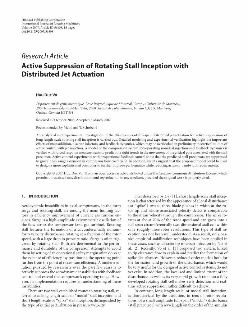
The MIT low-speed three stage axial compressor facility usedin this research was designed by Eastland [20] using a Pratt& Whitney research compressor. It has a constant tip diam-eter of 610 mm, a constant hub-to-tip ratio of 0.88, and itoperates at 2400 rpm. Further details of the compressor canbe found in Haynes et al. [7]. This compressor has been ex-tensively used in stall research, starting with Gamache andGreitzer [21] who measured reversed-flow performance andlater by Garnier et al. [22] who confirmed the presence ofmodal disturbances prior to rotating stall. This led to theuse of this compressor in active rotating stall stabilizationresearch by Haynes et al. [7] and Van Schalkwyk et al. [8].The facility was subsequently modified by Vo and Paduano[18] for experimental research with jet injection. A side viewand cross-section of the compression system are shown inFigure 1. The compressor, driven by an electric motor witha tachometer and a torque sensor, draws air through a bell-mouth inlet and two coarse screens. A set of eight pitotprobes and 16 circumferentially equally spaced hot wires areplaced at the midspan of the annulus upstream of the inletguide vanes (IGVs) for time-averaged and unsteady velocitymeasurements, respectively. An actuator ring is sandwichedbetween the IGVs and first rotor as shown in Figure 1. Time-averaged inlet total and exit static pressure measurements areobtained through the pitot probes and compressor exit end-wall static pressure taps, respectively. The air exiting the com-pressor enters a small annular exhaust plenum and passesthrough a conical valve used as a throttle to control the massflow (and thus the flow coefficient). The plenum volume issmall enough to preclude surge. The air subsequently exitsoutdoors via a dump plenum and a duct with several screensand an orifice plate, for mass flow measurement (to obtainflow coefficient).

For active control with jet actuation, the servo guidevanes used previously were replaced by twelve jet actuatorsdesigned by Diaz [19]. Each jet actuator consists of a valve

Huu Duc Vo 3

Exhaust fan(not used)

36” in. dia.

Orificeplate

Porousscreen Honeycomb

Porousscreen

ExhaustplenumConical

throttleCompressor

Sensorring

Distortiongenerator

Drive trainAxial compressortest facility(side view)

Drive motor

Servomotor

ValveInjectors

Hot wire

Flow

HubTip 63.5 mm

IGV

Jet actuator ring(front view) [19]

Opticalencoder

Servomotor

Valvebody

Mountingring

Injectors

Flow

Figure 1: MIT low-speed three-stage axial compressor test facility with jet actuation.

30◦

30◦

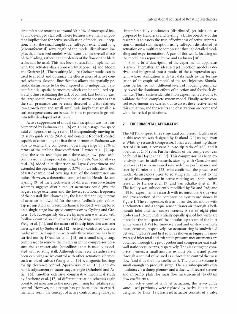
Figure 2: Injector design [19].

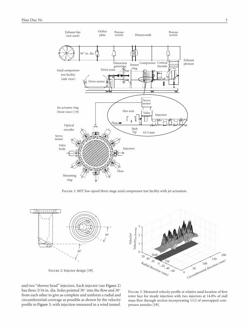
and two “shower head” injectors. Each injector (see Figure 2)has three 3/16 in. dia. holes pointed 30◦ into the flow and 30◦

from each other to give as complete and uniform a radial andcircumferential coverage as possible as shown by the velocityprofile in Figure 3, with injection measured in a wind tunnel.

200150

100

500

Circumferential direction (mm)

−60−40

−200

2040

20

Radial direction (mm)

0

1

2

3

Vel

ocit

y/V

eloc

ity n

obl

owin

g

Hub

Tip

Figure 3: Measured velocity profile at relative axial location of firstrotor face for steady injection with two injectors at 14.8% of stallmass flow through section incorporating 1/12 of unwrapped com-pressor annulus [19].


12 actuators(valves and servo

motors)

12

injectionrates

Fluid system

- Compressor-24 injectors- Ducts-16 hot wires

16

h.w.signals

Hot wireanemometers

(16)

16

h.w.outputs

Besselfilters (16)

12 servoamplifiers

12encoderoutputs

DMC 430motor controller

boards (4)

Control computer

- Highpass Butterworth filter- Converts h.w. readings to velocities- Computes discrete Fourier transform- Applies control law to each harmonic- Applies inverse discrete Fourier transformto obtain outputs to servo motors

12

motorcommands

16

filteredh.w.

outputs

Figure 4: Closed-loop control feedback configuration.

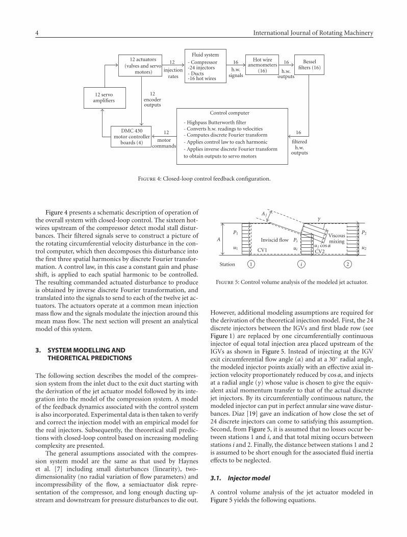
Figure 4 presents a schematic description of operation ofthe overall system with closed-loop control. The sixteen hot-wires upstream of the compressor detect modal stall distur-bances. Their filtered signals serve to construct a picture ofthe rotating circumferential velocity disturbance in the con-trol computer, which then decomposes this disturbance intothe first three spatial harmonics by discrete Fourier transfor-mation. A control law, in this case a constant gain and phaseshift, is applied to each spatial harmonic to be controlled.The resulting commanded actuated disturbance to produceis obtained by inverse discrete Fourier transformation, andtranslated into the signals to send to each of the twelve jet ac-tuators. The actuators operate at a common mean injectionmass flow and the signals modulate the injection around thismean mass flow. The next section will present an analyticalmodel of this system.

3. SYSTEM MODELLING ANDTHEORETICAL PREDICTIONS

The following section describes the model of the compres-sion system from the inlet duct to the exit duct starting withthe derivation of the jet actuator model followed by its inte-gration into the model of the compression system. A modelof the feedback dynamics associated with the control systemis also incorporated. Experimental data is then taken to verifyand correct the injection model with an empirical model forthe real injectors. Subsequently, the theoretical stall predic-tions with closed-loop control based on increasing modelingcomplexity are presented.

The general assumptions associated with the compres-sion system model are the same as that used by Hayneset al. [7] including small disturbances (linearity), two-dimensionality (no radial variation of flow parameters) andincompressibility of the flow, a semiactuator disk repre-sentation of the compressor, and long enough ducting up-stream and downstream for pressure disturbances to die out.

A

P1

u1

Inviscid flow Pi

uiCV1

Ajγ

uj cosαCV2

Viscousmixing

P2

u2

Station 1 i 2

Figure 5: Control volume analysis of the modeled jet actuator.

However, additional modeling assumptions are required forthe derivation of the theoretical injection model. First, the 24discrete injectors between the IGVs and first blade row (seeFigure 1) are replaced by one circumferentially continuousinjector of equal total injection area placed upstream of theIGVs as shown in Figure 5. Instead of injecting at the IGVexit circumferential flow angle (α) and at a 30◦ radial angle,the modeled injector points axially with an effective axial in-jection velocity proportionately reduced by cosα, and injectsat a radial angle (γ) whose value is chosen to give the equiv-alent axial momentum transfer to that of the actual discretejet injectors. By its circumferentially continuous nature, themodeled injector can put in perfect annular sine wave distur-bances. Diaz [19] gave an indication of how close the set of24 discrete injectors can come to satisfying this assumption.Second, from Figure 5, it is assumed that no losses occur be-tween stations 1 and i, and that total mixing occurs betweenstations i and 2. Finally, the distance between stations 1 and 2is assumed to be short enough for the associated fluid inertiaeffects to be neglected.

3.1. Injector model

A control volume analysis of the jet actuator modeled inFigure 5 yields the following equations.

Huu Duc Vo 5

From station 1 to station i:

continuity

ρuiAi = ρu1A(Ai = A− Aj cos γ

). (1)

Bernoulli

Pi +12ρu2

i = P1 +12ρu2

1. (2)

From station i to station 2 (CV2):

continuity

ρu2A = ρuj cosαAj + ρuiAi. (3)

Axial momentum

(Pi − P2

)A = −ρu2

i Ai − ρu2j cos2 αAj cos γ + ρu2

2A. (4)

The second term on the right-hand side of (4) repre-sents the effect of momentum addition, whereas the othertwo terms are the effect of mass addition. Combining (1)through (4), then simplifying and nondimensionalizing gives

φ2 = φ1 +(Aj

Acosα

)φj , (5)

Pt2 − Pt1ρU2

= −12Mφ2

2 − (N cosα)φ2φj +12

(R cos2 α

)φ2j ,

(6)

where R ≡ (Aj/A)(2 cos γ +N),

M ≡( (

Aj/A)

cos γ

1− (Aj/A) cos γ

)2

,

N ≡(Aj/A

)(1− 2

(Aj/A

)cos γ

)

(1− (Aj/A) cos γ

)2 ,

(7)

which in linearized form are

δφ2 = δφ1 +(Aj

Acosα

)δφj , (8)

δPt2 − δPt1ρU2

= −Xδφ2 − Yδφj , (9)

where X ≡Mφ2 +Nφj cosα, Y ≡ (Nφ2 − Rφj cosα) cosα.

3.2. Fluid system model

As explained in detail in [18], the fluid system modelis obtained essentially by adding the pressure rise acrossthe actuator (9) to the pressure rise across the compres-sor, as given by the Moore-Greitzer model with unsteadylosses [7, 9, 23, 24], and combined with the model’s

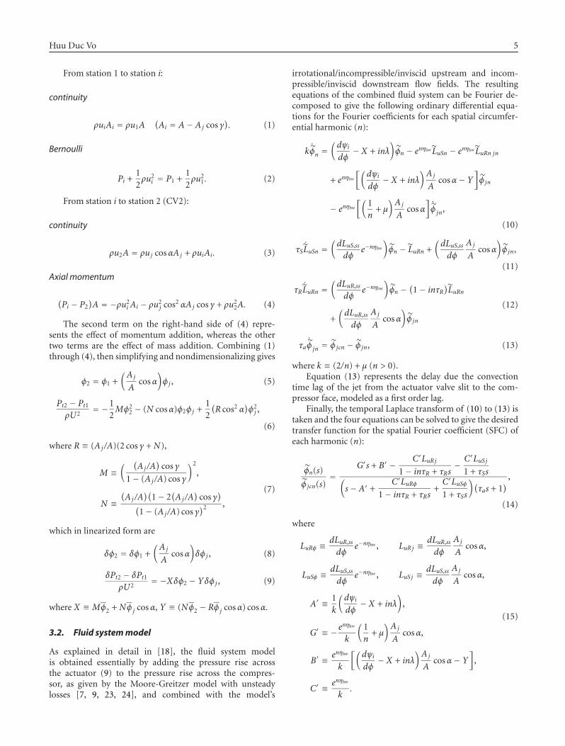
irrotational/incompressible/inviscid upstream and incom-pressible/inviscid downstream flow fields. The resultingequations of the combined fluid system can be Fourier de-composed to give the following ordinary differential equa-tions for the Fourier coefficients for each spatial circumfer-ential harmonic (n):

k˙φn =

(dψidφ

− X + inλ)φn − enηhw LuSn − enηhw LuRn jn

+ enηhw

[(dψidφ

− X + inλ)Aj

Acosα− Y

]φ jn

− enηhw

[(1n

+ μ)Aj

Acosα

]˙φjn,

(10)

τS˙LuSn =

(dLuS,ss

dφe−nηhw

)φn − LuRn +

(dLuS,ss

dφ

Aj

Acosα

)φ jn,

(11)

τR˙LuRn =

(dLuR,ss

dφe−nηhw

)φn −

(1− inτR

)LuRn

+(dLuR,ss

dφ

Aj

Acosα

)φ jn

(12)

τa˙φjn = φ jcn − φ jn, (13)

where k ≡ (2/n) + μ (n > 0).Equation (13) represents the delay due the convection

time lag of the jet from the actuator valve slit to the com-pressor face, modeled as a first order lag.

Finally, the temporal Laplace transform of (10) to (13) istaken and the four equations can be solved to give the desiredtransfer function for the spatial Fourier coefficient (SFC) ofeach harmonic (n):

φn(s)

φ jcn(s)=

G′s + B′ − C′LuRj1− inτR + τRs

− C′LuSj1 + τSs(

s− A′ +C′LuRφ

1− inτR + τRs+C′LuSφ1 + τSs

)(τas + 1

),

(14)

where

LuRφ ≡ dLuR,ss

dφe−nηhw , LuRj ≡ dLuR,ss

dφ

Aj

Acosα,

LuSφ ≡ dLuS,ss

dφe−nηhw , LuSj ≡ dLuS,ss

dφ

Aj

Acosα,

A′ ≡ 1k

(dψidφ

− X + inλ)

,

G′ ≡ −enηhw

k

(1n

+ μ)Aj

Acosα,

B′ ≡ enηhw

k

[(dψidφ

− X + inλ)Aj

Acosα− Y

],

C′ ≡ enηhw

k.

(15)


3.3. Modeling of control system dynamics

The theoretical study by Hendricks and Gysling [9] employsdirect feedback on a model of the fluid system similar tothe one derived above. However, to better predict the per-formance of actuation in practice, one should incorporateall the dynamics associated with the feedback loop. In thiscase, the pertinent control system dynamics are the feedbacktime delay, the highpass filters, the sample and hold dynam-ics of the discrete control process and the actuator dynam-ics. These dynamics, with the exception of the highpass filter,were modeled in detail by Haynes et al. [7], although someaspects are modified here to account for changes in the sys-tem.

First, the total feedback time delay from the ve-locity disturbance at the compressor face to the com-manded actuation sent to the servo motors can belumped and modeled by a pure time delay whose firstorder approximation is (16). Second, the only filterwhose dynamics can significantly affect the system is afirst-order Butterworth highpass filter with a cutoff fre-quency ( f ) of 0.1 Hz. It was used to correct for thedrift of the hot wires during the experiments. The fil-ter was implemented in the computer software and canbe modeled by (17). Third, the sample and hold dy-namics of the discrete-time control system was mod-eled in continuous time by Haynes [24] as (18). Fi-nally, the actuator dynamics incorporate the dynamicsfrom the commanded to actual servo motor position.This is modeled with the measured transfer functionin (19):

D(s) = 1− (τt/2)s

1 +(τt/2

)s

, (16)

F(s) = s

s + 2π f R/U, (17)

ZOH(s) = 11 +

(τ f /2

)s, (18)

A(s) = (s + 1.1934)(s + 0.3869± i0.3443)(s + 0.1824± i0.2933)(s + 1.5971± i3.0352)

• (s− 3.2229± i1.8607)(s + 3.2229± i1.8607)

.

(19)

To complete the model, the values of the parameters needto be obtained. Some, such as fluid inertias, can be calculatedfrom geometry. Others were obtained empirically. Such is thecase for the isentropic and actual compressor speedlines. Theformer is derived from the torque input and compressor ve-locity, the latter from pressure measurements. The differencebetween them is the total fluid loss Lu, with LR,ss = rLu andLS,ss = (1 − r)Lu, where r is the reaction of the compressor.

0.4 0.42 0.44 0.46 0.48 0.5 0.52 0.54 0.56 0.58

φd

0.9

0.92

0.94

0.96

0.98

1

1.02

1.04

1.06

1.08

1.1

ψ(a

ctu

ator

+co

mpr

esso

r)

Bottom to top curves:

mjet = 0%, 9.3%, 10.7% & 11.6% of mstall, no blowing

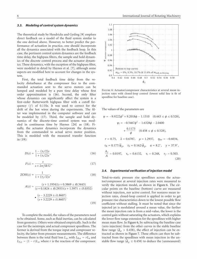
Figure 6: Actuator/compressor characteristics at several mean in-jection rates with closed-loop control (lowest solid line is fit ofspeedline for baseline case).

The values of the parameters are

ψ = −9.9222φ2 + 9.2018φ − 1.1310 (0.443 ≤ φ ≤ 0.528),

ψi = −0.5467φ2 − 1.6328φ − 2.0400

+0.1173φ

(0.458 ≤ φ ≤ 0.528),

r = 0.75, λ = 0.6787, μ = 1.2937, ηhw = −0.6034,

τR = 0.177/φd, τS = 0.162/φd, α = 8.2◦, γ = 37.9◦,

Aj

A= 0.0197, τa = 0.6132, τt = 0.248, τ f = 0.503.

(20)

3.4. Experimental verification of injection model

Total-to-static pressure rise speedlines across the actua-tor/compressor at several injection rates were measured toverify the injection model, as shown in Figure 6. The cir-cular points on the baseline (bottom) curve are measuredwithout injection, nor active control. For nonzero mean in-jection rates, closed-loop control is applied in order to getpressure rise characteristics down to the lowest possible flowcoefficient without stalling. It must be noted that since theinjected jet is modulated around a mean value, the fartherthe mean injection rate is from a mid-value, the lower is thecontrol gain without saturating the actuators, which explainsthe lower flow range extension for the speedlines with highermean mass flow. In Figure 6, by subtracting the baseline case(zero injection) from the other curves in the stable baselineflow range (φd > 0.458), the effect of injection can be ex-tracted as shown in Figure 7. These effects can then be sub-tracted from the speedlines with mean injection in the un-stable flow range (φd ≤ 0.458) to deduce the (unmeasured)

Huu Duc Vo 7

0.4 0.42 0.44 0.46 0.48 0.5 0.52 0.54 0.56 0.58

φd

0

0.01

0.02

0.03

0.04

0.05

0.06

0.07

0.08

0.09

0.1

ψje

t

Bottom to top curves:

mjet = 9.3%, 10.7% & 11.6% of mstall, no blowing

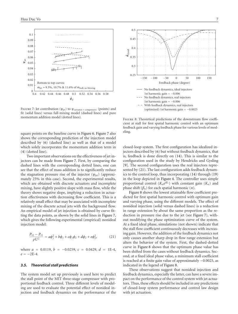
Figure 7: Jet contribution (ψjet) to ψ(actuator + compressor) (points) andfit (solid lines) versus full-mixing model (dashed lines) and puremomentum addition model (dotted lines).

square points on the baseline curve in Figure 6. Figure 7 alsoshows the corresponding prediction of the injection modeldescribed by (6) (dashed line) as well as that of a modelwhich solely incorporates the momentum addition term in(4) (dotted line).

Two important observations on the effectiveness of jet in-jectors can be made from Figure 7. First, by comparing thedashed lines with the corresponding dotted lines, one cansee that the effect of mass addition is to significantly reducethe stagnation pressure rise of the injector (ψjet) (approxi-mately 25% in this case). Second, the experimental results,which are obtained with discrete actuators and incompletemixing, have slightly positive slope with mass flow, while thetheory shows negative slope, implying a reduction in actua-tion effectiveness with decreasing flow coefficient. This is arelatively small effect that may be associated with incompletemixing of the discrete actual jets with the background flow.An empirical model of jet injection is obtained by curve fit-ting the data points, as shown by the solid lines in Figure 7,which gives the following experimental (empirical) nonidealinjection model:

Pt2 − Pt1ρU2

= aφ2j + bφj + cφjφ2 + dφ2 + eφ2

2, (21)

where a = 0.0119, b = −0.0259, c = 0.0429, d = 1E-4,e = −2E-4.

3.5. Theoretical stall predictions

The system model set up previously is used here to predictthe stall point of the MIT three-stage compressor with pro-portional feedback control. Three different levels of model-ing are used to evaluate the potential effect of nonideal in-jection and feedback dynamics on the performance of the

−150 −100 −50 0 50 100 150

Feedback phase (degree)

0.25

0.3

0.35

0.4

0.45

0.5

φd

,sta

ll

No feedback dynamics, ideal injectors1st harmonic gain = −0.006No feedback dynamics, real injectors1st harmonic gain = −0.006With feedback dynamics, real injectors(optimized) 1st harmonic gain = −0.0025

Figure 8: Theoretical predictions of the downstream flow coeffi-cient at stall for first spatial harmonic control with an optimumfeedback gain and varying feedback phase for various levels of mod-eling.

closed-loop system. The first configuration has idealized in-jectors described by (6) but without feedback dynamics, thatis, feedback is done directly on (14). This is similar to theconfiguration used in the study by Hendricks and Gysling[9]. The second configuration uses the real injectors repre-sented by (21). The last configuration adds feedback dynam-ics to the control loop, thus incorporating (14) through (19)in the loop depicted in Figure 4. The controller uses simpleproportional control (Kneiβn) with constant gain (Kn) andphase shift (βn) for each spatial harmonic (n).

Figure 8 shows the lowest attainable flow coefficient pre-dicted for first spatial harmonic control with optimum gainand varying phase, using the different models. The effect ofnonideal injection (solid versus dashed lines) is a reductionin range extension by about the same proportion as the re-duction in pressure rise due to the jet (see Figure 7), with-out modifying the phase optimization curve of the system.At a fixed ideal phase, simulations (not shown) indicate thatthe stall flow coefficient continuously decreases with increas-ing gain. However, the addition of the feedback dynamics notonly causes another sharp drop in flow range extension butalters the behavior of the system. First, the dashed-dottedcurve in Figure 8 shows that the optimum phase value hasbeen shifted from the cases without feedback dynamics. Sec-ond, at a fixed ideal phase value, a minimum stall coefficientis reached at a finite gain value of approximately −0.0025, asindicated in the legend of Figure 8.

These observations suggest that nonideal injection andfeedback dynamics, especially the latter, can have a severe im-pact on the performance of the control system with jet actua-tors. Thus, these effects should be included in any predictionsof closed-loop system performance and control law designwith jet actuation.


4. SYSTEM IDENTIFICATION

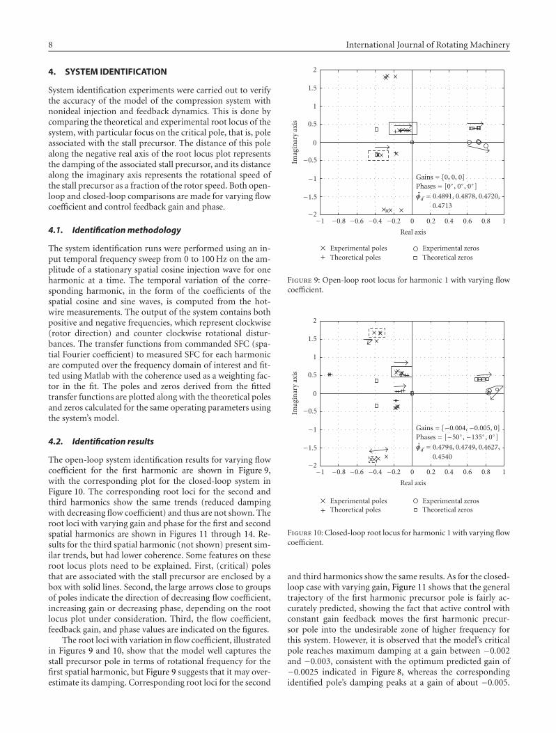
System identification experiments were carried out to verifythe accuracy of the model of the compression system withnonideal injection and feedback dynamics. This is done bycomparing the theoretical and experimental root locus of thesystem, with particular focus on the critical pole, that is, poleassociated with the stall precursor. The distance of this polealong the negative real axis of the root locus plot representsthe damping of the associated stall precursor, and its distancealong the imaginary axis represents the rotational speed ofthe stall precursor as a fraction of the rotor speed. Both open-loop and closed-loop comparisons are made for varying flowcoefficient and control feedback gain and phase.

4.1. Identification methodology

The system identification runs were performed using an in-put temporal frequency sweep from 0 to 100 Hz on the am-plitude of a stationary spatial cosine injection wave for oneharmonic at a time. The temporal variation of the corre-sponding harmonic, in the form of the coefficients of thespatial cosine and sine waves, is computed from the hot-wire measurements. The output of the system contains bothpositive and negative frequencies, which represent clockwise(rotor direction) and counter clockwise rotational distur-bances. The transfer functions from commanded SFC (spa-tial Fourier coefficient) to measured SFC for each harmonicare computed over the frequency domain of interest and fit-ted using Matlab with the coherence used as a weighting fac-tor in the fit. The poles and zeros derived from the fittedtransfer functions are plotted along with the theoretical polesand zeros calculated for the same operating parameters usingthe system’s model.

4.2. Identification results

The open-loop system identification results for varying flowcoefficient for the first harmonic are shown in Figure 9,with the corresponding plot for the closed-loop system inFigure 10. The corresponding root loci for the second andthird harmonics show the same trends (reduced dampingwith decreasing flow coefficient) and thus are not shown. Theroot loci with varying gain and phase for the first and secondspatial harmonics are shown in Figures 11 through 14. Re-sults for the third spatial harmonic (not shown) present sim-ilar trends, but had lower coherence. Some features on theseroot locus plots need to be explained. First, (critical) polesthat are associated with the stall precursor are enclosed by abox with solid lines. Second, the large arrows close to groupsof poles indicate the direction of decreasing flow coefficient,increasing gain or decreasing phase, depending on the rootlocus plot under consideration. Third, the flow coefficient,feedback gain, and phase values are indicated on the figures.

The root loci with variation in flow coefficient, illustratedin Figures 9 and 10, show that the model well captures thestall precursor pole in terms of rotational frequency for thefirst spatial harmonic, but Figure 9 suggests that it may over-estimate its damping. Corresponding root loci for the second

−1 −0.8 −0.6 −0.4 −0.2 0 0.2 0.4 0.6 0.8 1

Real axis

−2

−1.5

−1

−0.5

0

0.5

1

1.5

2

Imag

inar

yax

is

Gains = [0, 0, 0]Phases = [0◦, 0◦, 0◦]

φd = 0.4891, 0.4878, 0.4720,0.4713

Experimental polesTheoretical poles

Experimental zerosTheoretical zeros

Figure 9: Open-loop root locus for harmonic 1 with varying flowcoefficient.

−1 −0.8 −0.6 −0.4 −0.2 0 0.2 0.4 0.6 0.8 1

Real axis

−2

−1.5

−1

−0.5

0

0.5

1

1.5

2

Imag

inar

yax

is

Gains = [−0.004, −0.005, 0]Phases = [−50◦, −135◦, 0◦]

φd = 0.4794, 0.4749, 0.4627,0.4540



Figure 10: Closed-loop root locus for harmonic 1 with varying flowcoefficient.

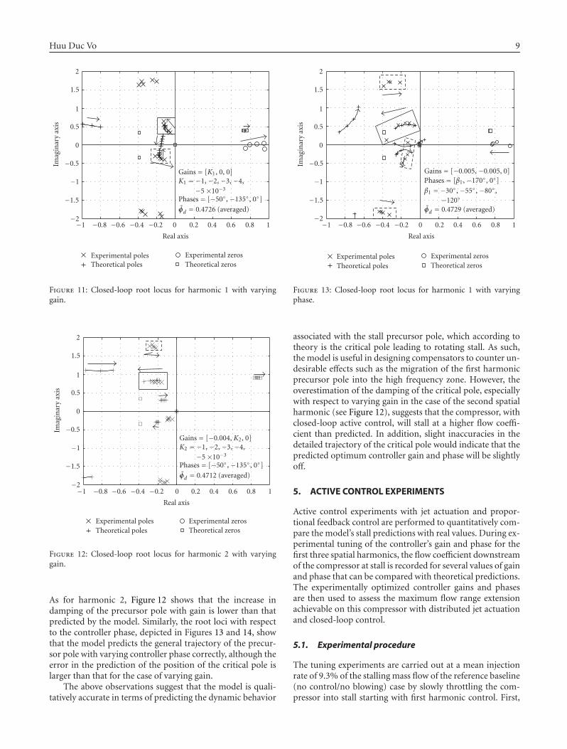
and third harmonics show the same results. As for the closed-loop case with varying gain, Figure 11 shows that the generaltrajectory of the first harmonic precursor pole is fairly ac-curately predicted, showing the fact that active control withconstant gain feedback moves the first harmonic precur-sor pole into the undesirable zone of higher frequency forthis system. However, it is observed that the model’s criticalpole reaches maximum damping at a gain between −0.002and −0.003, consistent with the optimum predicted gain of−0.0025 indicated in Figure 8, whereas the correspondingidentified pole’s damping peaks at a gain of about −0.005.

Huu Duc Vo 9

−1 −0.8 −0.6 −0.4 −0.2 0 0.2 0.4 0.6 0.8 1

Real axis

−2

−1.5

−1

−0.5

0

0.5

1

1.5

2

Imag

inar

yax

is

Gains = [K1, 0, 0]K1 = −1, −2, −3, −4,

−5 ×10−3

Phases = [−50◦, −135◦, 0◦]

φd = 0.4726 (averaged)



Figure 11: Closed-loop root locus for harmonic 1 with varyinggain.

−1 −0.8 −0.6 −0.4 −0.2 0 0.2 0.4 0.6 0.8 1

Real axis

−2

−1.5

−1

−0.5

0

0.5

1

1.5

2

Imag

inar

yax

is

Gains = [−0.004, K2, 0]K2 = −1, −2, −3, −4,

−5 ×10−3

Phases = [−50◦, −135◦, 0◦]




Figure 12: Closed-loop root locus for harmonic 2 with varyinggain.

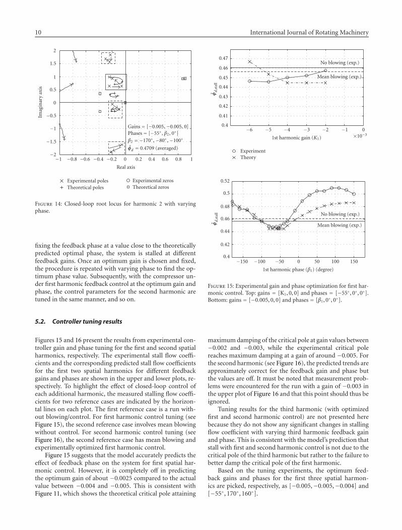
As for harmonic 2, Figure 12 shows that the increase indamping of the precursor pole with gain is lower than thatpredicted by the model. Similarly, the root loci with respectto the controller phase, depicted in Figures 13 and 14, showthat the model predicts the general trajectory of the precur-sor pole with varying controller phase correctly, although theerror in the prediction of the position of the critical pole islarger than that for the case of varying gain.

The above observations suggest that the model is quali-tatively accurate in terms of predicting the dynamic behavior

−1 −0.8 −0.6 −0.4 −0.2 0 0.2 0.4 0.6 0.8 1

Real axis

−2

−1.5

−1

−0.5

0

0.5

1

1.5

2

Imag

inar

yax

is

Gains = [−0.005, −0.005, 0]Phases = [β1, −170◦, 0◦]

β1 = −30◦, −55◦, −80◦,−120◦




Figure 13: Closed-loop root locus for harmonic 1 with varyingphase.

associated with the stall precursor pole, which according totheory is the critical pole leading to rotating stall. As such,the model is useful in designing compensators to counter un-desirable effects such as the migration of the first harmonicprecursor pole into the high frequency zone. However, theoverestimation of the damping of the critical pole, especiallywith respect to varying gain in the case of the second spatialharmonic (see Figure 12), suggests that the compressor, withclosed-loop active control, will stall at a higher flow coeffi-cient than predicted. In addition, slight inaccuracies in thedetailed trajectory of the critical pole would indicate that thepredicted optimum controller gain and phase will be slightlyoff.

5. ACTIVE CONTROL EXPERIMENTS

Active control experiments with jet actuation and propor-tional feedback control are performed to quantitatively com-pare the model’s stall predictions with real values. During ex-perimental tuning of the controller’s gain and phase for thefirst three spatial harmonics, the flow coefficient downstreamof the compressor at stall is recorded for several values of gainand phase that can be compared with theoretical predictions.The experimentally optimized controller gains and phasesare then used to assess the maximum flow range extensionachievable on this compressor with distributed jet actuationand closed-loop control.

5.1. Experimental procedure

The tuning experiments are carried out at a mean injectionrate of 9.3% of the stalling mass flow of the reference baseline(no control/no blowing) case by slowly throttling the com-pressor into stall starting with first harmonic control. First,


−1 −0.8 −0.6 −0.4 −0.2 0 0.2 0.4 0.6 0.8 1

Real axis

−2

−1.5

−1

−0.5

0

0.5

1

1.5

2

Imag

inar

yax

is

Gains = [−0.005, −0.005, 0]Phases = [−55◦, β2, 0◦]

β2 = −170◦, −80◦, −100◦




Figure 14: Closed-loop root locus for harmonic 2 with varyingphase.

fixing the feedback phase at a value close to the theoreticallypredicted optimal phase, the system is stalled at differentfeedback gains. Once an optimum gain is chosen and fixed,the procedure is repeated with varying phase to find the op-timum phase value. Subsequently, with the compressor un-der first harmonic feedback control at the optimum gain andphase, the control parameters for the second harmonic aretuned in the same manner, and so on.

5.2. Controller tuning results

Figures 15 and 16 present the results from experimental con-troller gain and phase tuning for the first and second spatialharmonics, respectively. The experimental stall flow coeffi-cients and the corresponding predicted stall flow coefficientsfor the first two spatial harmonics for different feedbackgains and phases are shown in the upper and lower plots, re-spectively. To highlight the effect of closed-loop control ofeach additional harmonic, the measured stalling flow coeffi-cients for two reference cases are indicated by the horizon-tal lines on each plot. The first reference case is a run with-out blowing/control. For first harmonic control tuning (seeFigure 15), the second reference case involves mean blowingwithout control. For second harmonic control tuning (seeFigure 16), the second reference case has mean blowing andexperimentally optimized first harmonic control.

Figure 15 suggests that the model accurately predicts theeffect of feedback phase on the system for first spatial har-monic control. However, it is completely off in predictingthe optimum gain of about −0.0025 compared to the actualvalue between −0.004 and −0.005. This is consistent withFigure 11, which shows the theoretical critical pole attaining

−6 −5 −4 −3 −2 −1 0×10−3

1st harmonic gain (K1)

0.4

0.41

0.42

0.43

0.44

0.45

0.46

0.47

φd

,sta

ll

ExperimentTheory

No blowing (exp.)

Mean blowing (exp.)

−150 −100 −50 0 50 100 150

1st harmonic phase (β1) (degree)

0.4

0.42

0.44

0.46

0.48

0.5

0.52

φd

,sta

ll No blowing (exp.)

Mean blowing (exp.)

Figure 15: Experimental gain and phase optimization for first har-monic control. Top: gains = [K1, 0, 0] and phases = [−55◦, 0◦, 0◦].Bottom: gains = [−0.005, 0, 0] and phases = [β1, 0◦, 0◦].

maximum damping of the critical pole at gain values between−0.002 and −0.003, while the experimental critical polereaches maximum damping at a gain of around −0.005. Forthe second harmonic (see Figure 16), the predicted trends areapproximately correct for the feedback gain and phase butthe values are off. It must be noted that measurement prob-lems were encountered for the run with a gain of −0.003 inthe upper plot of Figure 16 and that this point should thus beignored.

Tuning results for the third harmonic (with optimizedfirst and second harmonic control) are not presented herebecause they do not show any significant changes in stallingflow coefficient with varying third harmonic feedback gainand phase. This is consistent with the model’s prediction thatstall with first and second harmonic control is not due to thecritical pole of the third harmonic but rather to the failure tobetter damp the critical pole of the first harmonic.

Based on the tuning experiments, the optimum feed-back gains and phases for the first three spatial harmon-ics are picked, respectively, as [−0.005,−0.005,−0.004] and[−55◦, 170◦, 160◦].

Huu Duc Vo 11

−6 −5 −4 −3 −2 −1 0×10−3

2nd harmonic gain (K2)

0.4

0.41

0.42

0.43

0.44

0.45

0.46

0.47

φd

,sta

ll

ExperimentTheory

No blowing (exp.)

1st harmonic control (exp.)

−150 −100 −50 0 50 100 150

2nd harmonic phase (β2) (degree)

0.4

0.42

0.44

0.46

0.48

0.5

0.52

φd

,sta

ll No blowing (exp.)

1st harmonic control (exp.)

Figure 16: Experimental gain and phase optimization for secondharmonic control. Top: gains = [−0.005,K2, 0] and phases =[−55◦,−180◦, 0◦]. Bottom: gains = [−0.005,−0.005, 0] andphases = [−55◦,β2, 0◦].

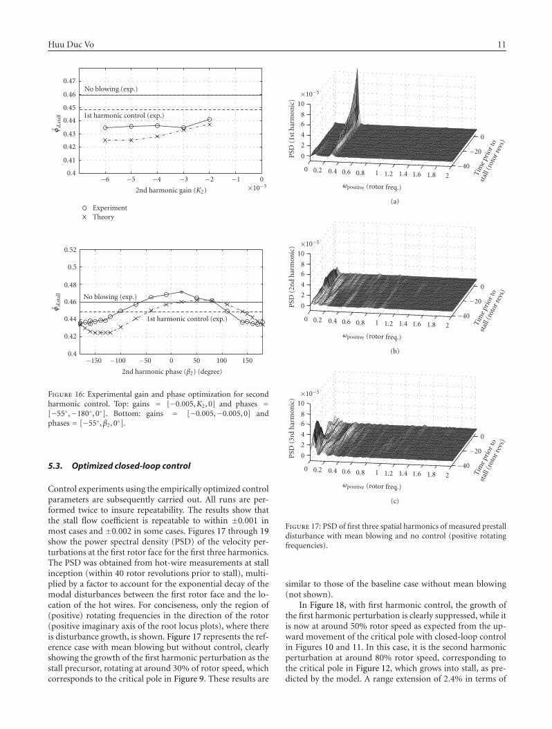
5.3. Optimized closed-loop control

Control experiments using the empirically optimized controlparameters are subsequently carried out. All runs are per-formed twice to insure repeatability. The results show thatthe stall flow coefficient is repeatable to within ±0.001 inmost cases and ±0.002 in some cases. Figures 17 through 19show the power spectral density (PSD) of the velocity per-turbations at the first rotor face for the first three harmonics.The PSD was obtained from hot-wire measurements at stallinception (within 40 rotor revolutions prior to stall), multi-plied by a factor to account for the exponential decay of themodal disturbances between the first rotor face and the lo-cation of the hot wires. For conciseness, only the region of(positive) rotating frequencies in the direction of the rotor(positive imaginary axis of the root locus plots), where thereis disturbance growth, is shown. Figure 17 represents the ref-erence case with mean blowing but without control, clearlyshowing the growth of the first harmonic perturbation as thestall precursor, rotating at around 30% of rotor speed, whichcorresponds to the critical pole in Figure 9. These results are

−40

−20

0

Tim

epr

ior t

o

stal

l (ro

tor r

evs)

0 0.2 0.4 0.6 0.8 1 1.2 1.4 1.6 1.8 2ωpositive (rotor freq.)

0

2

4

68

10×10−5

PSD

(1st

har

mon

ic)

(a)

−40

−20

0

Tim

epr

ior t

o

stal

l (ro

tor r

evs)


0

2

4

68

10×10−5

PSD

(2n

dh

arm

onic

)

(b)

−40

−20

0

Tim

epr

ior t

o

stal

l (ro

tor r

evs)


0

2

4

68

10×10−5

PSD

(3rd

har

mon

ic)

(c)

Figure 17: PSD of first three spatial harmonics of measured prestalldisturbance with mean blowing and no control (positive rotatingfrequencies).

similar to those of the baseline case without mean blowing(not shown).

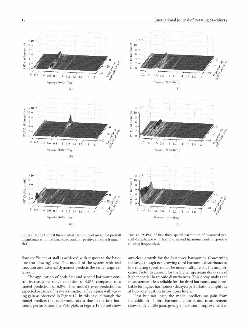
In Figure 18, with first harmonic control, the growth ofthe first harmonic perturbation is clearly suppressed, while itis now at around 50% rotor speed as expected from the up-ward movement of the critical pole with closed-loop controlin Figures 10 and 11. In this case, it is the second harmonicperturbation at around 80% rotor speed, corresponding tothe critical pole in Figure 12, which grows into stall, as pre-dicted by the model. A range extension of 2.4% in terms of


−40

−20

0

Tim

epr

ior t

o

stal

l (ro

tor r

evs)


0

2

4

68

10×10−5

PSD

(1st

har

mon

ic)

(a)

−40

−20

0

Tim

epr

ior t

o

stal

l (ro

tor r

evs)


0

2

4

68

10×10−5

PSD

(2n

dh

arm

onic

)

(b)

−40

−20

0

Tim

epr

ior t

o

stal

l (ro

tor r

evs)


0

2

4

68

10×10−5

PSD

(3rd

har

mon

ic)

(c)

Figure 18: PSD of first three spatial harmonics of measured prestalldisturbance with first harmonic control (positive rotating frequen-cies).

flow coefficient at stall is achieved with respect to the base-line (no blowing) case. The model of the system with realinjection and external dynamics predicts the same range ex-tension.

The application of both first and second harmonic con-trol increases the range extension to 4.8%, compared to amodel prediction of 6.8%. This model’s over-prediction isexpected because of its overestimation of damping with vary-ing gain as observed in Figure 12. In this case, although themodel predicts that stall would occur due to the first har-monic perturbation, the PSD plots in Figure 19 do not show

−40

−20

0

Tim

epr

ior t

o

stal

l (ro

tor r

evs)


0

2

4

68

10

×10−5

PSD

(1st

har

mon

ic)

(a)

−40

−20

0

Tim

epr

ior t

o

stal

l (ro

tor r

evs)


0

2

4

68

10

×10−5

PSD

(2n

dh

arm

onic

)

(b)

−40

−20

0

Tim

epr

ior t

o

stal

l (ro

tor r

evs)


0

2

4

68

10

×10−5

PSD

(3rd

har

mon

ic)

(c)

Figure 19: PSD of first three spatial harmonics of measured pre-stall disturbance with first and second harmonic control (positiverotating frequencies).

any clear growth for the first three harmonics. Concerningthe large, though nongrowing third harmonic disturbance atlow rotating speed, it may be noise multiplied by the amplifi-cation factor to account for the higher upstream decay rate ofhigher spatial harmonic disturbances. This decay makes themeasurements less reliable for the third harmonic and unre-liable for higher harmonics (decayed perturbation amplitudeat hot-wire location below noise levels).

Last but not least, the model predicts no gain fromthe addition of third harmonic control, and measurementshows only a little gain, giving a maximum improvement in

Huu Duc Vo 13

Table 1: Summary of experimental and theoretical stall flow coefficients with optimized closed-loop control.

Downstream flow coefficient at stall (φd,stall) [% decrease in φd,stall from baseline]

Description ExperimentModel w/o feedbackdynamics and idealinjection

Model w/o feedbackdynamics and realinjection

Model with feedbackdynamics and realinjection

No blowing (baseline) 0.458 0.456 0.456 0.456

Mean blowing, no control 0.455 [0.7%] 0.454 [0.4%] 0.461 [−1.1%] 0.461 [−1.1%]

1st harmonic control 0.447 [2.4%] 0.436 [4.3%] 0.445 [2.4%] 0.445 [2.4%]

1st and 2nd harmonic control 0.436 [4.8%] 0.402 [11.8%] 0.414 [9.2%] 0.425 [6.8%]

1st, 2nd, and 3rd harmonic control 0.433 [5.5%] 0.385 [15.6%] 0.409 [10.3%] 0.425 [6.8%]

0.42 0.43 0.44 0.45 0.46 0.47 0.48 0.49 0.5 0.51 0.52

φd

0.96

0.98

1

1.02

1.04

1.06

ψ(a

ctu

ator

+co

mpr

esso

r)

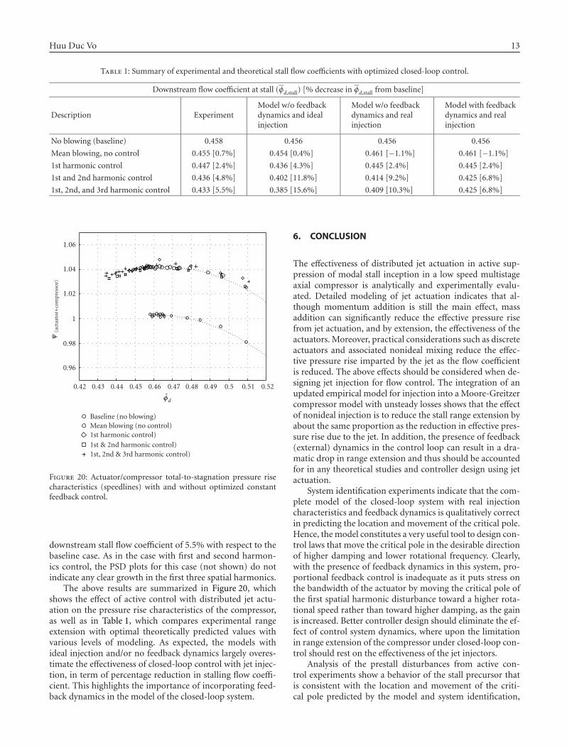
Baseline (no blowing)Mean blowing (no control)1st harmonic control)1st & 2nd harmonic control)1st, 2nd & 3rd harmonic control)

Figure 20: Actuator/compressor total-to-stagnation pressure risecharacteristics (speedlines) with and without optimized constantfeedback control.

downstream stall flow coefficient of 5.5% with respect to thebaseline case. As in the case with first and second harmon-ics control, the PSD plots for this case (not shown) do notindicate any clear growth in the first three spatial harmonics.

The above results are summarized in Figure 20, whichshows the effect of active control with distributed jet actu-ation on the pressure rise characteristics of the compressor,as well as in Table 1, which compares experimental rangeextension with optimal theoretically predicted values withvarious levels of modeling. As expected, the models withideal injection and/or no feedback dynamics largely overes-timate the effectiveness of closed-loop control with jet injec-tion, in term of percentage reduction in stalling flow coeffi-cient. This highlights the importance of incorporating feed-back dynamics in the model of the closed-loop system.

6. CONCLUSION

The effectiveness of distributed jet actuation in active sup-pression of modal stall inception in a low speed multistageaxial compressor is analytically and experimentally evalu-ated. Detailed modeling of jet actuation indicates that al-though momentum addition is still the main effect, massaddition can significantly reduce the effective pressure risefrom jet actuation, and by extension, the effectiveness of theactuators. Moreover, practical considerations such as discreteactuators and associated nonideal mixing reduce the effec-tive pressure rise imparted by the jet as the flow coefficientis reduced. The above effects should be considered when de-signing jet injection for flow control. The integration of anupdated empirical model for injection into a Moore-Greitzercompressor model with unsteady losses shows that the effectof nonideal injection is to reduce the stall range extension byabout the same proportion as the reduction in effective pres-sure rise due to the jet. In addition, the presence of feedback(external) dynamics in the control loop can result in a dra-matic drop in range extension and thus should be accountedfor in any theoretical studies and controller design using jetactuation.

System identification experiments indicate that the com-plete model of the closed-loop system with real injectioncharacteristics and feedback dynamics is qualitatively correctin predicting the location and movement of the critical pole.Hence, the model constitutes a very useful tool to design con-trol laws that move the critical pole in the desirable directionof higher damping and lower rotational frequency. Clearly,with the presence of feedback dynamics in this system, pro-portional feedback control is inadequate as it puts stress onthe bandwidth of the actuator by moving the critical pole ofthe first spatial harmonic disturbance toward a higher rota-tional speed rather than toward higher damping, as the gainis increased. Better controller design should eliminate the ef-fect of control system dynamics, where upon the limitationin range extension of the compressor under closed-loop con-trol should rest on the effectiveness of the jet injectors.

Analysis of the prestall disturbances from active con-trol experiments show a behavior of the stall precursor thatis consistent with the location and movement of the criti-cal pole predicted by the model and system identification,


especially for control of the lower spatial harmonics. In termsof stall delay, the trends are right but, as expected from theover prediction of the damping by the model, the stall predic-tions are slightly optimistic. The best result achieved with jetactuation in this system with proportional feedback controlis a range extension of 5.5% in downstream flow coefficientcompared with a theoretically predicted maximum of 6.8%.However, a more sophisticated controller that can mitigatethe negative effects of the feedback dynamics could improvethe range extension with this actuation scheme.

NOMENCLATURE

Symbols

A: Area

A(s): Actuator dynamics

D(s): Feedback time delay transfer function

F(s): Butterworth filter transfer function

f : Cut-off frequency of F(s)

Kn: Controller feedback gain

Lu: Pressure loss across the compressor due to vis-cous losses

LuR: Pressure loss across the rotors due to viscouslosses

LuS: Pressure loss across the stators due to viscouslosses

m: Mass flow

n: harmonic number

Pt : Total pressure

Ps: Static pressure

PSD: Power spectral density

R: Mean compressor radius

r: Compressor reaction

s: Laplace transform variable

t: Time

U : Mean rotor blade velocity

ZOH(s): Discrete sampling dynamics transfer function

α: Injection angle in the annular plane with re-spect to axial direction

βn: Controller feedback phase

γ: Injection angle in the radial plane with respectto axial direction

η: Nondimensional axial position with respect tocompressor face

λ: Rotor fluid inertia

μ: Total fluid inertia in the compressor

ρ: Air density

ξ: Nondimensional time

Φ: Local flow potential

φ: Axial flow coefficient, (axial velocity)/U

φ: annulus-averaged axial flow coefficient

ξ: Nondimensional time

τa: Jet convection time lag constant

τ f : Sampling (ZOH(s)) time constant

τt : Feedback delay (D(s)) time constant

ω: Temporal frequency

φn: nth spatial Fourier coefficient of flow coefficient dis-turbance δφ

φd: φ downstream of the jet actuator

ψ: Steady-state stagnation-to-static pressure rise coef-ficient, (Ps,out − Pt,in)/ρU2

ψi: Steady-state isentropic stagnation-to-static pressurerise coefficient

ψjet: Stagnation pressure rise coefficient due to jetactuation

Operator, superscripts, and subscripts

δ( ): Small perturbation

(∼): Spatial Fourier coefficient

(•): Derivative with respect to nondimensionaltime (ξ)

( )∗: Complex conjugate

( )c: Pertaining to the input

( )I : Station (i) in Figure 5

( ) j : Pertaining to the jet

( )n: nth harmonic

( )hw: Hot wires

( )u: Upstream of actuator

( )d: Downstream of actuator

( ),ss: Steady state

ACKNOWLEDGMENTS

This work was carried out while the author was at the GasTurbine Laboratory, Massachusetts Institute of Technology,Cambridge, MA. The author wishes to thank Dr. J. D. Pad-uano, Professor A. H. Epstein, and Dr. H. J. Weigl for theiradvice, and Dr. J. Protz, Dr. C. Van Schalkwyk and the tech-nicians of the MIT Gas Turbine Laboratory for their help insetting up the experimental facilities. This work was spon-sored by the U.S. Air Force Office of Scientific Research, Dr.J. McMicheal, Technical Manager, whose support is gratefullyacknowledged.

REFERENCES

[1] I. J. Day, “Stall inception in axial flow compressors,” Journal ofTurbomachinery, vol. 115, no. 1, pp. 1–9, 1993.

[2] C. Nie, G. Xu, X. Cheng, and J. Chen, “Micro air injection andits unsteady response in a low-speed axial compressor,” Journalof Turbomachinery, vol. 124, no. 4, pp. 572–579, 2002.

Huu Duc Vo 15

[3] H. D. Vo, C. S. Tan, and E. M. Greitzer, “Criteria for spikeinitiated rotating stall,” in Proceedings of the ASME TurboExpo—Gas Turbie Technology: Focus for the Future, pp. 155–165, Reno-Tahoe, Nev, USA, June 2005, ASME Paper GT2005-68374.

[4] F. K. Moore, “Theory of rotating stall of multistage ax-ial compressors—part I: small disturbances—part II: finitedisturbances—part III: limit cycles,” Journal of Engineering forGas Turbines and Power, vol. 106, no. 2, pp. 313–336, 1984.

[5] F. K. Moore and E. M. Greitzer, “Theory of post-stall tran-sients in axial compression systems—part I: development ofequations,” Journal of Engineering for Gas Turbines and Power,vol. 108, no. 1, pp. 68–76, 1986.

[6] J. D. Paduano, A. H. Epstein, L. Valavani, J. P. Longley, E. M.Greitzer, and G. R. Guenette, “Active control of rotating stallin a low-speed axial compressor,” Journal of Turbomachinery,vol. 115, no. 1, pp. 48–56, 1993.

[7] J. M. Haynes, G. J. Hendricks, and A. H. Epstein, “Active sta-bilization of rotating stall in a three-stage axial compressor,”Journal of Turbomachinery, vol. 116, no. 2, pp. 226–239, 1994.

[8] C. M. Van Schalkwyk, J. D. Paduano, E. M. Greitzer, andA. H. Epstein, “Active stabilization of axial compressors withcircumferential inlet distortion,” Journal of Turbomachinery,vol. 120, no. 3, pp. 431–439, 1998.

[9] G. J. Hendricks and D. L. Gysling, “Theoretical study ofsensor-actuator schemes for rotating stall control,” Journal ofPropulsion and Power, vol. 10, no. 1, pp. 101–109, 1994.

[10] D. L. Gysling and E. M. Greitzer, “Dynamic control of rotat-ing stall in axial flow compressors using aeromechanical feed-back,” Journal of Turbomachinery, vol. 117, no. 3, pp. 307–319,1995.

[11] H. J. Weigl, J. D. Paduano, L. G. Frechette, et al., “Active stabi-lization of rotating stall and surge in a transonic single-stageaxial compressor,” Journal of Turbomachinery, vol. 120, no. 4,pp. 625–636, 1998.

[12] K. L. Suder, M. D. Hathaway, S. A. Thorp, A. J. Strazisar, andM. B. Bright, “Compressor stability enhancement using dis-crete tip injection,” Journal of Turbomachinery, vol. 123, no. 1,pp. 14–23, 2001.

[13] R. D’Andrea, R. L. Behnken, and R. M. Murray, “Rotating stallcontrol of an axial flow compressor using pulsed air injection,”Journal of Turbomachinery, vol. 119, no. 4, pp. 742–752, 1997.

[14] S. Yeung, Y. Wang, and R. M. Murray, “Bleed valve rate re-quirements evaluation in rotating stall control on axial com-pressors,” Journal of Propulsion and Power, vol. 16, no. 5, pp.781–791, 2000.

[15] Z. S. Spakovszky, J. D. Paduano, R. Larsonneur, A. Traxler, andM. M. Bright, “Tip clearance actuation with magnetic bearingsfor high-speed compressor stall control,” Journal of Turboma-chinery, vol. 123, no. 3, pp. 464–472, 2001.

[16] M. T. Schobeiri and M. Attia, “Active control of compressorinstability and surge by stator blades adjustment,” Journal ofPropulsion and Power, vol. 19, no. 2, pp. 312–317, 2003.

[17] L. G. Frechette, O. G. McGee, and M. B. Graf, “Tailored struc-tural design and aeromechanical control of axial compressorstall—part II: evaluation of approaches,” Journal of Turboma-chinery, vol. 126, no. 1, pp. 63–72, 2004.

[18] H. D. Vo and J. D. Paduano, “Experimental development ofa jet injection model for rotating stall control,” in Proceedingsof the International Gas Turbine & Aeroengine Congress & Ex-hibition, p. 11, Stockholm, Sweden, June 1998, ASME Paper98-GT-308.

[19] D. S. Diaz, “Design of a jet actuator for active control of rotat-ing stall,” S.M. thesis, Department of Aeronautics and Astro-nautics, MIT, Cambridge, Mass, USA, 1994.

[20] A. H. J. Eastland, “Investigation of compressor performance inrotating stall,” MIT GTL Report 164, MIT, Cambridge, Mass,USA, 1982.

[21] R. N. Gamache and E. M. Greitzer, “Reverse flow in multistageaxial compressors,” Journal of Propulsion and Power, vol. 6,no. 4, pp. 461–473, 1990.

[22] V. H. Garnier, A. H. Epstein, and E. M. Greitzer, “Rotatingwaves as a stall inception indication in axial compressors,”Journal of Turbomachinery, vol. 113, no. 2, pp. 290–302, 1991.

[23] J. D. Paduano, “Active control of rotating stall in axial com-pressors,” MIT GTL Report 208, MIT, Cambridge, Mass, USA,1992.

[24] J. M. Haynes, “Active control of rotating stall in a three-stageaxial compressor,” MIT GTL Report 218, MIT, Cambridge,Mass, USA, 1993.

International Journal of

AerospaceEngineeringHindawi Publishing Corporationhttp://www.hindawi.com Volume 2010

RoboticsJournal of

Hindawi Publishing Corporationhttp://www.hindawi.com Volume 2014


Active and Passive Electronic Components

Control Scienceand Engineering

Journal of



RotatingMachinery


Hindawi Publishing Corporation http://www.hindawi.com

Journal ofEngineeringVolume 2014

Submit your manuscripts athttp://www.hindawi.com

VLSI Design



Shock and Vibration


Civil EngineeringAdvances in

Acoustics and VibrationAdvances in



Electrical and Computer Engineering

Journal of

Advances inOptoElectronics

Hindawi Publishing Corporation http://www.hindawi.com

Volume 2014

The Scientific World JournalHindawi Publishing Corporation http://www.hindawi.com Volume 2014

SensorsJournal of


Modelling & Simulation in EngineeringHindawi Publishing Corporation http://www.hindawi.com Volume 2014


Chemical EngineeringInternational Journal of Antennas and

Propagation




Navigation and Observation



DistributedSensor Networks


Active Suppression of Rotating Stall Inception with...

Documents

Transcript of Active Suppression of Rotating Stall Inception with...