ACTIVE STEREO VISION: DEPTH PERCEPTION FOR NAVIGATION ...
163
ACTIVE STEREO VISION: DEPTH PERCEPTION FOR NAVIGATION, ENVIRONMENTAL MAP FORMATION AND OBJECT RECOGNITION A THESIS SUBMITTED TO THE GRADUATE SCHOOL OF NATURAL AND APPLIED SCIENCES OF THE MIDDLE EAST TECHNICAL UNIVERSITY BY LKAY ULUSOY IN PARTIAL FULLFILLMENT OF THE REQUIREMENTS FOR THE DEGREE OF DOCTOR OF PHILOSOPHY IN THE DEPARTMENT OF ELECTRICAL AND ELECTRONICS ENGINEERING SEPTEMBER 2003
Transcript of ACTIVE STEREO VISION: DEPTH PERCEPTION FOR NAVIGATION ...

ACTIVE STEREO VISION: DEPTH PERCEPTION FOR NAVIGATION,
ENVIRONMENTAL MAP FORMATION AND OBJECT RECOGNITION
A THESIS SUBMITTED TO THE GRADUATE SCHOOL OF NATURAL AND APPLIED SCIENCES
OF THE MIDDLE EAST TECHNICAL UNIVERSITY
BY �
LKAY ULUSOY
IN PARTIAL FULLFILLMENT OF THE REQUIREMENTS FOR THE
DEGREE OF
DOCTOR OF PHILOSOPHY
IN
THE DEPARTMENT OF ELECTRICAL AND ELECTRONICS
ENGINEERING
SEPTEMBER 2003

Approval of the Graduate School of Natural and Applied Sciences
_______________________
Prof. Dr. Canan Özgen Director
I certify that this thesis satisfies all the requirements as a thesis for the degree of Doctor of Philosophy.
_______________________
Prof. Dr. Mübeccel Demirekler Head of Department
This is to certify that we have read this thesis and that in our opinion it is fully adequate, in scope and quality, as a thesis for the degree of Doctor of Philosophy.
_______________________
Prof. Dr. U� ur Halıcı Supervisor
Examining Committee Members
Prof. Dr. Kemal Leblebicio� lu _______________________
Prof. Dr. U� ur Halıcı _______________________
Prof. Dr. Hasan Güran _______________________
Assoc. Prof. Dr. Volkan Atalay _______________________
Prof. Dr. Erhan Nalçacı _______________________

iii
ABSTRACT
ACTIVE STEREO VISION: DEPTH PERCEPTION FOR NAVIGATION,
ENVIRONMENTAL MAP FORMATION AND OBJECT RECOGNITION
Ulusoy, �lkay
Ph. D., Department of Electrical and Electronics Engineering
Supervisor: Prof. Dr. U� ur Halıcı
September 2003, 148 pages
In very few mobile robotic applications stereo vision based navigation and mapping
is used because dealing with stereo images is very hard and very time consuming.
Despite all the problems, stereo vision still becomes one of the most important
resources of knowing the world for a mobile robot because imaging provides much
more information than most other sensors. Real robotic applications are very
complicated because besides the problems of finding how the robot should behave
to complete the task at hand, the problems faced while controlling the robot’s
internal parameters bring high computational load. Thus, finding the strategy to be
followed in a simulated world and then applying this on real robot for real
applications is preferable. In this study, we describe an algorithm for object

iv
recognition and cognitive map formation using stereo image data in a 3D virtual
world where 3D objects and a robot with active stereo imaging system are
simulated. Stereo imaging system is simulated so that the actual human visual
system properties are parameterized. Only the stereo images obtained from this
world are supplied to the virtual robot. By applying our disparity algorithm, depth
map for the current stereo view is extracted. Using the depth information for the
current view, a cognitive map of the environment is updated gradually while the
virtual agent is exploring the environment. The agent explores its environment in an
intelligent way using the current view and environmental map information obtained
up to date. Also, during exploration if a new object is observed, the robot turns
around it, obtains stereo images from different directions and extracts the model of
the object in 3D. Using the available set of possible objects, it recognizes the object.
Keywords: stereo vision, active vision, disparity, depth perception, environmental
map, object recognition

v
ÖZ
AKT�F STEREO GÖRME:
�LERLEME, ÇEVRESEL HAR
�TA ÇIKARMA VE
NESNE TANIMA AMAÇLARI
�Ç
�N DER
�NL
�K ALGILANMASI
Ulusoy, �lkay
Doktora, Elektrik ve Elektronik Mühendisli � i Bölümü
Tez Yöneticisi: Prof. Dr. U� ur Halıcı
Eylul 2003, 148 sayfa
Stereo görme analizi çok zor ve zaman alıcı oldu� u için, robot çalı� malarında çok
sık tercih edilen bir yöntem de� ildir. Buna ra� men, hareketli bir robot için çevrenin
daha detaylı bilinmesi açısından stereo görüntüleme en temel kaynak olarak tercih
edilmeye ba� lanmı� tır. Bunun en temel nedeni, görüntülemenin analizi çok zor
olmasına ra� men di � er sensörlere nazaran çok daha fazla bilgi sa� lıyor olmasıdır.
Gerçek robot uygulamaları çok karma� ıktır. Bu nedenle, robotun nasıl davranması
gerekti � inin bulunması amaçlanıyorsa öncelikle simülasyonlar üzerinde çalı� ıp daha
sonra bulunan stratejinin gerçek robot üzerinde uygulanması tercih edilen bir
yöntemdir. Bu çalı� mada, üç boyutlu sanal bir ortam olu� turulmu� tur. Bu sanal
ortamda üç boyutlu nesneler ve aktif stereo görme sistemine sahip sanal bir robot

vi
yer almaktadır. Bu sanal ortamdan alınan stereo görüntüler kullanılarak sanal
robotun nesne tanıması ve çevresel harita çıkarması hedeflenmi � tir. Stereo
görüntüleme sistemi, gerçek insan görme sistemi özelliklerine göre simüle
edilmi � tir. Sanal robot, sadece stereo görüntüleri kullanmaktadır. Farklılık
algoritmamız kullanılarak stereo görüntülerden o anki görme alanı için derinlik
bilgisi çıkarılmaktadır. Robot akıllı bir � ekilde etrafı tararken, derinlik bilgisi
kullanılarak kognitif harita sürekli doldurulmaktadır. Robot, ortamda ilerlemeyi o
anki görsel bilgi ve o ana kadar olu� turulmu� kognitif harita yardımıyla
gerçekle� tirmektedir. Aynı zamanda robot, ortamda dola� ırken yeni bir nesne ile
kar� ıla� ırsa, nesnenin etrafında dönerek farklı yönlerden stereo görüntüsünü
çekmekte ve üç boyutlu modelini çıkarmaktadır. Daha önceden tanımlanmı�
olabilecek nesneler arasından, görmü� oldu� u nesneyi üç boyutlu yapı bilgisinden
çıkarmaktadır.
Anahtar Kelimeler: stereo görme, aktif görme, farklılık, derinlik algısı, çevresel
harita çıkarmak, nesne tanıma

vii
To My Father, Mother, Brother and Lovely Daughter

viii
ACKNOWLEDGEMENTS
I would like to express my gratitude to my supervisor Prof. Dr. U� ur Halıcı for her
guidance and support throughout the research. I would also like to thank to Prof. Dr.
Kemal Leblebicio� lu, Asst. Prof. Dr. Volkan Atalay and Prof. Dr. Edwin Hancock
for their contributions.
I would like to acknowledge TUB�TAK-BAYG for the scholarship that covered my
studies at the University of York, UK and thank to both my supervisor and
TUB�TAK for providing me such a possibility.

ix
TABLE OF CONTENTS
ABSTRACT............................................................................................................. III
ÖZ.............................................................................................................................. V
DEDICATION.................................................................................................... .VI
ACKNOWLEDGEMENTS.................................................................................. VIII
LIST OF FIGURES.................................................................................................XII
LIST OF TABLES................................................................................................. XV
CHAPTER
1. INTRODUCTION.................................................................................................. 1
1.1 Problem Definition and Motivation ............................................................... 1
1.2 Contribution ................................................................................................... 6
1.3 Organization of the Thesis............................................................................. 9
2. LITERATURE REVIEW..................................................................................... 11
2.1 Vision for Mobile Robots............................................................................. 11
2.1.1 Map-based Navigation ............................................................................. 11
2.1.2 Map-less Navigation ................................................................................ 12
2.1.3 Map Building............................................................................................ 14
2.2 Stereo Vision for Mobile Robots................................................................. 15
2.3 Stereo Algorithms........................................................................................ 18
2.3.1 Dense Stereo Algorithms......................................................................... 18
2.3.2 Sparse Stereo Algorithms......................................................................... 21
2.3.3 Biological Stereo Algorithms................................................................... 24
2.3.4 Probabilistic stereo algorithms................................................................. 28
2.4 Reconstruction from Multiple Images ......................................................... 29
2.5 Biological Navigation and Robotic Applications......................................... 30

x
2.5.1 Local Navigation...................................................................................... 31
2.5.2 Way Finding............................................................................................. 32
2.5.3 Cognitive Maps........................................................................................ 34
2.6 Robotic Mapping.......................................................................................... 35
2.6.1 Taxonomy of robotic mapping................................................................. 35
2.6.2 Problems in Robotic Mapping ................................................................. 39
2.6.3 Simultaneous Localization and Mapping................................................. 41
2.7 Virtual Environment Applications............................................................... 43
3. BIOLOGICAL STEREO VISION WITH MULTI SCALE PHASE BASED
FEATURES.............................................................................................................. 45
3.1 Introduction and Motivation......................................................................... 45
3.2 Feature Extraction by Population Coding Method....................................... 46
3.3 Feature Extraction Using Steerable Filters................................................... 50
3.4 Finding Corresponding Pairs Using Multi-scale Phase................................ 56
3.5 Finding Disparity and Depth........................................................................ 57
3.6 Complexity of the Algorithm....................................................................... 69
3.7 Probabilistic Model of the Disparity Algorithm .......................................... 71
3.7.1 Probability Density Estimation of Phase Differences by von Mises Model
71
3.7.2 Probability of Being a Pair ....................................................................... 79
3.7.3 Validation of the Probabilistic Model ...................................................... 81
3.8 Summary and Conclusion ............................................................................ 85
4. APPLICATION OF OUR ACTIVE STEREO VISION ALGORITHM ON A
VIRTUAL ROBOT FOR COGNITIVE MAP FORMATION AND OBJECT
RECOGNITION IN A VIRTUAL ENVIRONMENT............................................. 88
4.1 Introduction.................................................................................................. 88
4.2 Design and Implementation Details of the Simulation Software................. 91
4.3 Camera Controller ........................................................................................ 96
4.4 Active Vision and Cognitive Map Construction.......................................... 97
4.5 Object Recognition..................................................................................... 102

xi
4.6 Results and Conclusion.............................................................................. 110
5. CONCLUSION.................................................................................................. 116
REFERENCES....................................................................................................... 120
APPENDICES
A. DEPTH PERCEPTION IN HUMAN VISUAL SYSTEM ............................... 128
A.1 Pictorial Depth Cues................................................................................... 128
A.1.1 Occlusion (Interposition).................................................................... 128
A.1.2 Linear Perspective.............................................................................. 129
A.1.3 Relative familiar size.......................................................................... 131
A.1.4 Focus, Depth of Field and Accommodation ...................................... 132
A.2 Binocular disparity (Stereopsis) ................................................................. 134
B. GEOMETRY FILE FORMAT.......................................................................... 136
C. A SAMPLE CAMERACONTROLLER PLUGIN ........................................... 146
D. CAMERACONTROLLER.H............................................................................ 146
E. C++ SCRIPT FOR RGB TO HSV CONVERSION.......................................... 148

xii
LIST OF FIGURES
FIGURE
1. Modules of the whole system.............................................................................................5
2. Flow chart of the stereo vision system. ............................................................................10
3. Different models for disparity encoding cells: a. Position shift model, b. Phase shift
model, c. Hybrid model. (Picture is taken from [19]) ..................................................26
4. a,b. Stereo image pair (Blocks 1) taken from CMU database, c,d. Corresponding feature
points with orientation given in color scale. In this case population coding method has
been used......................................................................................................................50
5. The template filter used in analysis. a. The real part which is the 4th derivative of
Gaussian, b. The Imaginary part which is a steerable approximation to the Hilbert
transform of the real part..............................................................................................52
6. Feature points obtained by steerable filtering for the Blocks 1 stereo image pair given in
Figure 4. The orientation is given in color scale..........................................................53
7. Feature points extracted using filters at different number of scales. a. Single scale where
width of the filter is 6 pixels, b. Single scale where width of the filter is 18 pixels, c.
Three scales where filter widths are 6, 12 and 18 pixels, d. Five scales where filter
widths are 6,10,14,18,22 pixels....................................................................................55
8. Stereo camera projection system......................................................................................58
9. Disparity estimated for the Blocks 1 image pair. .............................................................59
10. Fine tuning. Feature points are numbered starting from the left-most one through the
right-most one and given in the x-axis of the plot. y-axis shows the disparity where
rough disparity is given with (* ) and fine tuned disparity given with line. .................60
11. a. Left image, b. Right image, c. Disparity. Stereo images (Blocks 2) are taken from
CMU stereo database. ..................................................................................................62
xiii
12. a Left image, b. Right image, c. Disparity. Stereo images (Venus stereo pair) are taken
from Middlebury Stereo webpage................................................................................63
13. a. Left image, b. Right image, c. Disparity. Stereo images (Sawtooth stereo pair) are
taken from Middlebury Stereo webpage......................................................................64
14. a. Left image, b. Right image, c. Disparity. Stereo images (Tsukuba stereo pair) are
taken from Middlebury Stereo webpage......................................................................65
15. Fine tuning. Feature points are numbered starting from the left-most one through the
right-most one and given in the x-axis of the plot. y-axis shows the disparity where
rough disparity is given with (* ) and fine tuned disparity given with line. .................67
16. Disparity calculated for Sawtooth stereo pair using: a. Single scale where filter width is
six pixels, b. Three scales where filter widths are 6, 12 and 18 pixels. .......................68
17. Mixture of von Mises models for the correct pair phase differences. a, c, e. Components
of the mixture model for scale 1, 2 and 3 respectively, b, d, f. Mixture model and
histogram of phase differences for scale 1, 2 and 3 respectively.................................78
18. Results for Venus stereo pair. a. Disparity found by the method in Section 3.5, b.
Disparity found by the probabilistic model described in Section 3.6. .........................80
19. Results for Block stereo pair. a. Disparity found by the method in Section 3.5, b.
Disparity found by the probabilistic model described in Section 3.6. .........................82
20. Results for Sawtooth stereo pair. a. Disparity found by the method in Section 3.5, b.
Disparity found by the probabilistic model described in Section 3.6. .........................83
21. Results for Tsukuba stereo pair. a. Disparity found by the method in Section 3.5, b.
Disparity found by the probabilistic model described in Section 3.6. .........................84
22. A screen shot from the virtual environment. A farm cottage and different type of trees
are seen. In the upper left and right panes left and right eye views are shown
respectively. In the lower left and right panes top and front views are shown
respectively. Below of the bottom panes, there are tab based dialog boxes. ...............92
23. Interface for displaying feature point information. Locations of feature points for the
cottage are shown on the left camera view as black dots and disparities found are
shown on the right camera view in colors....................................................................93
24. Top-view with camera and target controls.....................................................................96
25. States of camera controller DLL. .................................................................................100
26. Flowchart of the map construction system...................................................................101
xiv
27. 3D cognitive map. x- and z- axis are the width and depth of the environment
respectively and y-axis is for height above the ground. Only the grids for which the
belief of being occupied are high are shown here. Others are given zero values i.e. not
occupied. ....................................................................................................................102
28. a. Location and color information stored in each grid for an apple tree in the cognitive
map, b. Cognitive map grids for the top of the apple tree, c. Cognitive map grids for
the body of the apple tree...........................................................................................104
29. a. Location and color information stored in each grid for a pine tree in the cognitive
map, b. Cognitive map grids for the top of the pine tree, c. Cognitive map grids for the
body of the pine tree...................................................................................................105
30. Labeled occupancy.......................................................................................................109
31. a. Virtual environment with three different object very far away from each other, b.
Computed 3D map, c. Occupancy (top view of 3D map) with labeled objects. ........110
32. a. Virtual environment with three objects of the same type, b. Computed 3D map, c.
Occupancy (top view of 3D map) with labeled objects. ............................................112
33. An illustration showing the effect of occlusion............................................................129
34. An illustration showing linear perspective...................................................................130
35. Relative size as a cue. Which one of the balloons looks closer?..................................131
36. Accommodation. Blurred image. .................................................................................132
37. Accommodation. Focused image. ................................................................................133
38. Uncrossed disparity ......................................................................................................134
39. Crossed disparity..........................................................................................................135

xv
LIST OF TABLES
TABLE
1. Success rate of the algorithm for different stereo pairs....................................................66
2. Parameters of the algorithm effective for complexity......................................................70
3. Success rate of the probabilistic model for different image pairs. ...................................81
4. Parameters used in the program. ....................................................................................115

1
CHAPTER 1
INTRODUCTION
1.1 Problem Definition and Motivation
In this thesis the main goal is to develop a biologically inspired stereo vision system
and to use this system in a robotic application where human-like activities such as
cognitive map formation and object recognition are performed.
Navigation could not be achieved unless distance information is obtained. For
other activities of human such as object recognition, shape extraction, etc., some
other cues such as silhouette, shading, texture, etc., could also be used but for
navigation and localization depth information is crucial.
Although monocular cues, such as previous familiarity, interposition, linear and
size perspective, distribution of shadows and illumination and motion parallax, are
effective for depth perception (See Appendix A for detailed information about
depth perception), for many species with frontally located eyes including humans,
binocular disparity provides a powerful and highly quantitative cue to near field
(<100 ft) depth perception. Binocular disparity refers to a small positional
difference between corresponding images features in the two eyes, and arises
because the two eyes are separated horizontally. Depth perception based upon
binocular disparities is known as stereopsis.
In many robotics applications depth is usually extracted by proximity sensors
such as ultrasound or laser scanners. However, cameras have several desirable

2
properties compared to these proximity sensors. They are low cost sensors that
provide a huge amount of information, they are easy to set-up and they are passive
so that vision based navigation systems do not suffer from the interferences often
observed when using active sound- or light-based proximity sensors.
For depth extraction, at least a stereo camera system is necessary. However,
since dealing with stereo images is very hard and very time consuming, only in
some recent mobile robotic applications stereovision is used. In spite of the fact that
there are big problems in dealing with stereo images, stereovision is becoming one
of the most important resources of knowing the world for a mobile robot. One of the
reasons is that although imaging is very difficult to handle, it provides much more
information of the world than most other sensors. The other reason is that with
recent improvements in the hardware, time consuming applications are becoming
faster and easier. Moreover, if robots are deployed in populated environment, it
makes sense to base the perceptional skills on vision as humans do [98].
There are some commercial products as been used in [61]. However these
require special hardware. Since on-body real-time systems are required for mobile
robotics, using only standard PC hardware and simple image capture card system
instead of systems which require special hardware is preferred [42].
Higher vertebrates like humans can perform navigation extending beyond
sensory horizon. They can make short-cuts and can find other route to destination if
the route they are following was blocked. This is called survey navigation and for
such navigation some form of spatial representation is necessary. Higher vertebrates
appear to construct representations (sometimes referred to as cognitive maps) which
encode spatial relations between relevant locations in their environment.
Hippocampus is known to be the place in the brain for such a representation. Many
studies investigated hippocampus of rat brain and cognitive maps are modeled
based on these physiological findings [49].
Real robotic applications are very complicated because besides the problems of
finding how the robot should behave to complete the task at hand, the problems

3
faced while controlling the robot’s internal parameters bring high computational
load. Thus, first working in a simulated environment in order to find the strategy to
be followed by the robot and then applying this on real robotic applications is
preferable. Especially intelligent way finding, path planning and mapping
algorithms are developed in simulated environments [41, 80, 90, 97, 79, 49].
Biologically inspired active vision system is also implemented in such a virtual
environment in [90].
In this study we develop a multi-scale phase based disparity algorithm for the
purpose of depth estimation which is very important for human navigation. Since
dealing with stereovision and robot control at the same time is very hard, we also
apply our stereovision algorithm in a simulated world with simulated cameras and
objects where the goal is to construct three dimensional (3D) map of the
environment. Then, in the future studies our algorithm can be applied on real robots.
In robotic research various systems for map construction have been proposed.
Some uses metric measurements to construct the map. Some only extracts the
topology of the environment [88]. Although metric maps suffer from big size, due to
accuracy embedded in such maps they provide better localization for the robot.
Because of this reason we have chosen grid-based mapping which is also a metric
mapping. Some studies prefer robot centered maps versus world centered maps.
However, since world centered maps are easier to construct we choose world
centered maps. But such maps suffer from movement errors due to slippery and
odometry errors, since this kind of errors add up in time. But since we use stereo
vision in our map construction algorithm we assume that ego-motion extraction and
localization could be performed easily. Thus, world centered maps can be
constructed without major error. In our future studies algorithms for ego-motion
extraction and localization for stereo-vision will be developed for real robotic
applications in natural environments. All these different mapping methods and
problems coming with them are explained in Chapter 2. In this thesis we construct a

4
world centric, grid based cognitive map which is very important for higher
vertebrate survey navigation.
Our virtual world is a computer simulation of a very simple 3D environment. In
this environment there is an agent which has a stereo imaging system modeled with
the properties of human eye. There are also 3D objects each having two parts which
are either sphere, ellipsoid, cylinder or cone of any size. Some of the 3D objects are
as follows: a sphere on top of a cylinder is an apple tree, a cone on top of a small
radius cylinder is a pine tree, a cone on top of a large radius cylinder is a cottage,
etc. The agent uses only the stereo image pairs obtained form this virtual world and
explores its environment based on some heuristics. It simultaneously builds up a 3D
map and recognizes the objects it observes during exploration.
The schema of the complete system is given in Figure 1. Our system is
composed of two main modules: 1) Simulation module (SM) where virtual
environment exists, 2) Processor module (PM) where all kinds of control activities
are achieved. Also, processor module is composed of two sub modules: 1) Map
formation and object recognition sub-module, 2) Navigation and camera controller
sub-module.

5
Figure 1 Modules of the whole system.
The system works as follows: First, 2D stereo images are rendered from the 3D
virtual world and passed to PM. Then, using our multi-scale phase based disparity
algorithm, depth map is extracted for the current view and environmental map is
updated. From the environmental map formed up to date, navigation destination is
decided and cameras are controlled. Finally, new camera locations and parameters
are passed to the SM. All these activities are recursively done in a continuous
manner until all of the environment is explored. Each time a new depth estimate is
calculated, environmental map is updated and each time all the information about a
new object is fully extracted, object is recognized. Thus, map formation and object
recognition sub-module and navigation and camera controller sub-module works in
parallel.
Our human-like stereo vision system does not require special hardware. Only a
standard PC and a frame grabber would be enough for obtaining stereo images in
SIMULATION
MODULE (Virtual Environment)
NAVIGATION
AND CAMERA CONTROLLER
SUB-MODULE
2D stereo image pair
Camera positions and parameters
MAP FORMATION
AND OBJECT RECOGNITION
SUB-MODULE
PROCESSOR MODULE

6
natural environments. We inspired from biological binocular cell models and use
steerable filters to extract interest points, called feature points in this thesis. The
feature used in order to match corresponding feature points is the multi-scale phase
information. The flow chart which summarizes our stereo vision algorithm is shown
in Figure 2. Using steerable filters, feature points are extracted from both of the
stereo image pair. Using the oriented filters at different scales, we obtain multi-scale
phase and magnitude information at each feature point. Then corresponding pairs
are matched based on multi-scale phase similarity. Finally, depth and 3D location
information are calculated from disparity with the help of known camera parameters
and location information.
1.2 Contr ibution
In this study we propose a biological model for feature based disparity estimation
and use this system in robotic applications. First of all a biological disparity
estimation model is proposed. Then our disparity algorithm is modeled
probabilistically. Finally our disparity algorithm is used on a virtual robot with
stereo vision in a 3D virtual world in order to construct 3D map of the environment
and recognize objects around.
The usual method for feature point matching is to compare vector of filter
responses at different scales and orientations which requires many operations since
the compared vector could be very large [99, 40]. Later, Lüdtke, Wilson and
Hancock uses population coding method in order to estimate a single orientation
value for each feature point which would make the comparison easier. In their work
they inspired from hyper-column structure of the visual cortex. When population
coding is used to represent the convolution responses of the filter bank, the outputs
of only a small number of filters need to be combined in order to achieve a
considerable improvement of the precision of orientation estimation. However in
their case, they use only a single scale in finding the feature points and estimating
the orientation values. In this study we use steerable filters at three different scales

7
in finding our feature points and estimating orientations. When a small number of
oriented filter responses are used to obtain responses at other orientations this is
called steerable filtering. In this study we used the method of [26] in designing our
steerable filters. Also, by using filters tuned at various frequencies, feature points
having high information content at different local frequencies are selected.
Although feature points extracted from image pairs are sparse, since they are the
points of high contrast edges in various scales that define the bounding contours of
objects, they still prove to be informative.
Since phase is very sensitive to spatial differences and at the same time very
stable to lighting, orientation and scale deformations, using phase information in
order to find correspondences between feature points provides reliable solutions.
Unfortunately, there are image locations where phase is singular and can not be
reliably used [38-39]. Such points are the locations where local frequencies at these
points are very different from the filter tuning. In this study, by selecting feature
points using multi-scale analysis, performing phase comparisons at multiple scales
and by using magnitude confidence information we overcome these difficulties. The
confidence weighting is used to augment phase information with information
concerning the magnitude of the steerable filtered image to improve the
correspondence method.
Using phase in correspondence matching is also biologically grounded. The
reason for this is that simple binocular cells occur in pairs that are in quadrature
phase. In physiological modeling of binocular cells, phase-based disparity methods
are highly appreciated. Physiological phase-based models can be classified into
two: 1. Disparity is estimated from local phase difference between left and right
images based on Fourier theorem as been done in [84]. 2. Phase shift model of
binocular cells: Receptive fields of binocular cells have phase differences and this is
used in energy models [25, 76]. Both models have some limitations. Because, when
phase is used, disparity estimation is reliable only for the disparity values less than
half of the filter wavelength. Nature has a solution for this problem: In experimental

8
studies, it is observed that there are also binocular cells which have similar
receptive fields but located at different positions [25]. There are biological cell
models based on this finding and they are called position-shift models. In position
shift models of binocular cells, receptive fields are similar but positioned at
different locations. By this model a large range of disparities can be estimated. In
[38-39] hybrid model which has both position shift and phase shift is proposed.
However it also has same kind of limitation. In this study, two routes to locating
feature-point correspondences are explored. Inspired from the position shift model,
corresponding pairs are found by checking the phase vector similarity along
epipolar line. Rough disparity values are obtained and a large range of disparities
can be calculated, but to a limited accuracy. Inspired from the phase shift model,
local phase difference is used in calculating subpixel disparity which has the
accuracy less than one pixel. Fine tuning is performed without encountering the
quarter cycle limit. This tuning scheme also allows a continuum of disparity
estimates to be obtained.
In [8] stability of phase for some deformations is investigated and in a later study
[9] they applied their method to feature matching and conclude that in order to be
sure for stability of phase through scale, multi-scaling should be included. The use
of multiple scales is also biologically plausible. The reason for this is that binocular
cells, which are encoding disparity, are sensitive to different spatial wavelengths. In
all the studies given above, first disparities at different scales are computed and then
the results are pooled in order to obtain a single disparity map. However in this
study, we include multiple scaling at the beginning both in extracting features and
in matching. Disparity is estimated only once using multi-scale phase directly in
matching.
In the probabilistic modeling of our matching algorithm, mixture of von Mises
distributions is used. The distribution of phase differences between matched pairs at
each scale for Venus stereo image pair is modeled and the models at all scales are
tested on other stereo pairs. The important thing here is that although modeling is

9
done by using Venus stereo pair data only, it works fine for many other images. By
this probabilistic model, we not only reach a higher success rate for many image
pairs, but bring flexibility to the disparity search region.
Finally, the disparity estimation is applied to map construction and object
recognition in a virtual world. Other than the usually known 2D occupancy grid
method, a 3D map is constructed in this study. Our heuristic exploration strategy
uses the advantage of active vision property. The importance of using vision in
robotic applications is also emphasized by including an object recognition task. In
recognizing objects, first of all point cloud belonging to an object is considered.
Then this point cloud is segmented into two parts by using proximity and color
similarity. Then surfaces are fit to each part and finally object is recognized from
the shape of the parts.
1.3 Organization of the Thesis
In Chapter 2 literature review of vision for mobile robot navigation, stereo vision
for mobile robot, various disparity algorithms, biological and robotic navigation,
robotic map formation, virtual environments and 3D reconstruction from multiple
images are summarized. In Chapter 3 our biological disparity algorithm is given.
Results are also presented in the same chapter. Our probabilistic model for disparity
algorithm is also explained in Chapter 3. In Chapter 4 application of our
stereovision to a virtual environment for the purpose of 3D cognitive map formation
and object recognition is explained thoroughly. The related results are also given in
this chapter. Chapter 5 is the conclusion chapter.

10
Figure 2 Flow chart of the stereo vision system.
LEFT IMAGE RIGHT IMAGE
STEERABLE FILTERING-
FEATURE POINT EXTRACTION
FILTERING AT EDGE POINTS WITH
ORIENTED FILTERS- FEATURE EXTRACTION
MATCHING AND
DISPARITY ESTIMATION
DEPTH COMPUTATION
EDGE, ORIENTATION
DISPARITY
DEPTH AND 3D LOCATION INFORMATION
CAMERA LOCATION AND PARAMETERS
MULTI-SCALE PHASE AND MAGNITUDE
11
CHAPTER 2
LITERATURE REVIEW
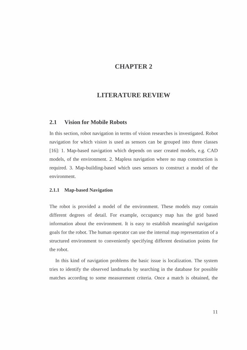
2.1 Vision for Mobile Robots
In this section, robot navigation in terms of vision researches is investigated. Robot
navigation for which vision is used as sensors can be grouped into three classes
[16]: 1. Map-based navigation which depends on user created models, e.g. CAD
models, of the environment. 2. Mapless navigation where no map construction is
required. 3. Map-building-based which uses sensors to construct a model of the
environment.
2.1.1 Map-based Navigation
The robot is provided a model of the environment. These models may contain
different degrees of detail. For example, occupancy map has the grid based
information about the environment. It is easy to establish meaningful navigation
goals for the robot. The human operator can use the internal map representation of a
structured environment to conveniently specifying different destination points for
the robot.
In this kind of navigation problems the basic issue is localization. The system
tries to identify the observed landmarks by searching in the database for possible
matches according to some measurement criteria. Once a match is obtained, the

12
system needs to calculate its position as a function of the observed landmarks and
their positions in the database.
In probabilistic FINALE [60], the uncertainty in the position and orientation on
the plane of the robot is represented by a Gaussian distribution and, thus, the
uncertainty at each location of the robot is characterized by mean and covariance. In
topological NEURONAV [58], a graph topologically representing a layout of the
hallways is used for driving the vision process. Two modules, hallway follower and
landmark detector are implemented using an ensemble of neural networks.
Most of the earlier methods use a single camera and a range sensor. In [73]
monocular, trinocular vision based and laser based robot localization are compared
and comparable precision levels are attained. Since vision provides much more
information it is preferred by many recent studies although vision poses more
complex matching problems than laser. In [98] images are retrieved and a data base
is formed and then Monte-Carlo localization is used to find the similarity between
the current image and the data base. In [89] triclops camera system is used and ego
motion of the robot is calculated from the scale invariant features detected and
matched through successive frames.
2.1.2 Map-less Navigation
Navigation is achieved without any prior description of the environment. No maps
are ever created. Most robotic systems are limited to essentially just roaming in
mapless systems. In most cases the robot only has access to a few sequences of
images that help it to get to its destination or a few predefined images of target
goals that it can use to track and pursue. Navigation using optical flow, appearance
based matching, object recognition are some examples.
In navigation using optical flow, motion parallax is more useful and features
such as “ time-to-crash” are more relevant than distance when it is necessary to jump
over an obstacle. In [65] N images of the same scene are obtained by N cameras

13
each having a different focal length where focal length is categorized in 3 steps, i.e.
far, medium, close. Cameras are positioned together such that they see the same
perspective. The scene is divided into regions and the best focus for each region is
found by computing sharpness (i.e. intensity differences between all horizontally
neighboring pixels). Thus, each region is assigned far, medium or close. The robot
moves using the farness or closeness information in the regions of the image. In
[45] active vision based control is used for collision avoidance as well as
maintenance of clearance in a priori unknown textured environments. Change in
image quality measure, which is defined in their study, is used in a fuzzy logic
control.
In navigation using appearance based matching, memorizing the environment is
done by storing images or templates of the environment and associating those
images with commands or controls. In [30] the set of local views for a given
panoramic image defines a “place” in the environment. Each place is associated
with a direction (azimuth) to the goal. Finally, a neural network is used to learn this
association and during actual navigation, it provides the controls that take the robot
to its final destination. In [55] after a sequence of images is stored, the robot is
required to repeat the same trajectory. The system compares the currently observed
image with the images in the sequence database using correlation. The displacement
in pixels between the view image and the template image is then used for steering.
In [66], the robot is manually driven in the obstacle free hallway and expectation
maps are rendered from the hallway model at regular intervals. First, the robot
renders an expectation image using its current best estimate of where its present
location is. Next, the model edges extracted from the expectation image are
compared and matched with the edges extracted from the camera image through an
extended Kalman filter. The Kalman filter automatically then yields updated values
for the location and the orientation of the robot. Obstacles are found from the
difference of vertical edges in the camera image and the expectation map
immediately after each exercise in self localization.

14
In navigation using object recognition, instead of using appearance based
approaches to memorize and recall locations, a symbolic navigation approach such
as “go to the door” is used in [44]. In [5] vision based autonomous vehicle requires
the ability to focus on the important features in an input scene. Task dependent
emphasizing or deemphasizing is modeled by a neural network where hidden layer
keeps important information for the task only.
2.1.3 Map Building
Automated or semi automated robots could explore their environment and build an
internal representation of it. Occupancy grids are the basic methods. They allow
measurements from multiple sensors to be incorporated. Even uncertainties can be
embedded in the map. The extent to which the resulting geometry can be relied
upon for subsequent navigation depends naturally on the accuracy of robot
odometry and sensor uncertainties during map construction.
Additionally for large scale and complex spaces, the resulting representations
may not be computationally efficient for path planning, localization, etc. Instead
topological representations of space can be used [23]. These representations often
have local metrical information embedded for node recognition and to facilitate
navigational decision making after a map is constructed. Various proposed
approaches differ with respect to what constitutes a node in a graph-based
description of the space, how a node may be distinguished from other neighboring
nodes, the effect of sensor uncertainty, the compactness of the representation. Major
difficulty is the recognition of nodes previously visited.
In metrical approaches, on the other hand, if the odometry and the sensors are
sufficiently accurate, the computed distances between the different features of space
help in identifying places previously visited. The best of the occupancy grid based
and topology based approaches are combined in [91] but using range sensors only.
In [48] stereo camera system is used besides the laser range finder in map
construction, object recognition and navigation. But the environment is a simple

15
indoor one and predefined special features are needed. In [42], on body depth
generation system which requires only a PC and an image card is implemented.
After the formation of the map, the next problem is the localization. In [70] a
map similarity measure is formed using the probability distribution of the distance
from each occupied cell in the local map that is computed at the current robot
position to the closest occupied cell in a previously computed map of the
environment. This probability distribution function is used in a likelihood function
for each robot pose. Some recent studies perform simultaneous mapping and
localization as in [89] and [14].
2.2 Stereo Vision for Mobile Robots
Stereo cameras used in robotic applications are built to simulate the way human
visual system works. Human visual system, having all its amazing powers, helps us
to see the world, study the world and understand the world and is also very
powerful in telling the depth of objects in the scene. Human visual system interprets
depth in sensed images using both physiological and psychological cues. The
physiological depth cues include accommodation, convergence, binocular parallax,
and monocular movement parallax. The psychological cues are retinal image size,
linear perspective, texture gradient, overlapping, aerial perspective, and shades and
shadows. Among these cues, only convergence and binocular parallax are binocular
depth cues (requiring both eyes to be open), while all others are monocular (one eye
only). Detailed explanation of human depth perception can be found in Appendix A.
Although stereo vision systems loses almost all the monocular cues as well as the
binocular cue such as convergence and performs poorly so far compared to human
visual system, stereo vision still becomes one of the most important resources of
knowing the world for a mobile robot. One of the main reasons is that although it is
very difficult to handle, imaging the world provides yet much more information of
the world than most other sensors. Another reason is that as mobile robots are built
to simulate or help human beings, it is important to make them look and work as

16
humans. With better and better stereo algorithms, advances in image processing,
computer vision, artificial intelligence, etc., improvements in hardware, and with
the belief that robot should act as human beings, we can anticipate that stereo vision
will be one of the most widely used sensors for mobile robots.
In a standard setting of stereo imaging used on a robot, two cameras are bound
together with a certain displacement. These stereo cameras have parallel optical
axes and most likely the same focal lengths. In most application scenarios, by
calculating the disparity map between the two captured images, stereo vision helps
recover depth information of the environment, which can then be used by mobile
robots to avoid obstacles, construct map, localize itself and recognize visual
commands.
Stereo vision for mobile robots has some specific requirements. The first
requirement is that the algorithm has to be real-time. The reason for this
requirement can be miscellaneous, for example, to avoid obstacles or to recognize
gestures. Second, mobile robots tend to move around and take pictures. This means
the stereo algorithm needs to handle image sequences. This provides the algorithm a
better chance to get the correct disparity map or refine it. Third, mobile robots are
typically moving on a plane ground. To avoid obstacles on the ground, the disparity
map can be calculated based on the plane ground (called horopter). Fourth, stereo is
not the only sensor on a mobile robot. Fusion of multiple sensors needs to be
studied to best estimate the environment the robot is in.
Some robotic applications where stereo is used are listed as follows:
Real time stereo processing and obstacle detection (horopter based stereo):
Many approaches can be used to do stereo in real time especially when accuracy is
not very important. For example, a hierarchical pyramid of the two stereo pair can
be built and the matching can be refined step-by-step from coarse to fine level. As
fine level disparity can be initialized by the coarse level disparity, this can improve
the speed greatly. Another way to speed up stereo is to down sample the images, as
well as the disparity levels. For mobile robot, sometimes ignoring the details may
17
actually help increase the stability of the system, especially when the task of the
stereo does not require a lot of accuracy.
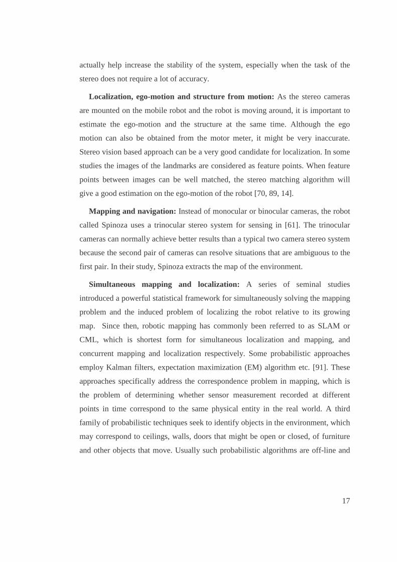
Localization, ego-motion and structure from motion: As the stereo cameras
are mounted on the mobile robot and the robot is moving around, it is important to
estimate the ego-motion and the structure at the same time. Although the ego
motion can also be obtained from the motor meter, it might be very inaccurate.
Stereo vision based approach can be a very good candidate for localization. In some
studies the images of the landmarks are considered as feature points. When feature
points between images can be well matched, the stereo matching algorithm will
give a good estimation on the ego-motion of the robot [70, 89, 14].
Mapping and navigation: Instead of monocular or binocular cameras, the robot
called Spinoza uses a trinocular stereo system for sensing in [61]. The trinocular
cameras can normally achieve better results than a typical two camera stereo system
because the second pair of cameras can resolve situations that are ambiguous to the
first pair. In their study, Spinoza extracts the map of the environment.
Simultaneous mapping and localization: A series of seminal studies
introduced a powerful statistical framework for simultaneously solving the mapping
problem and the induced problem of localizing the robot relative to its growing
map. Since then, robotic mapping has commonly been referred to as SLAM or
CML, which is shortest form for simultaneous localization and mapping, and
concurrent mapping and localization respectively. Some probabilistic approaches
employ Kalman filters, expectation maximization (EM) algorithm etc. [91]. These
approaches specifically address the correspondence problem in mapping, which is
the problem of determining whether sensor measurement recorded at different
points in time correspond to the same physical entity in the real world. A third
family of probabilistic techniques seek to identify objects in the environment, which
may correspond to ceilings, walls, doors that might be open or closed, of furniture
and other objects that move. Usually such probabilistic algorithms are off-line and

18
can not be run in real time. In most recent studies map construction and localization
and/or ego-motion extraction are simultaneously studied [89, 14].
2.3 Stereo Algor ithms
2.3.1 Dense Stereo Algor ithms
Recently there were some efforts by Scharstein and Szeliski [85] who tried to
provide a common test bed for evaluating different stereo algorithms. In their work,
they measure the performances of different algorithms based on known ground truth
data. Four pairs of images were used in their system (Sawtooth, Tsukuba, Venus
and Map). The two criteria they used were:
RMS (root mean square) error (measured in disparity units) between the
computed disparity map dC(x,y) and the ground truth map dT(x,y):
2
1
),(
2),(),(1
��
�
�
��
�
�� −=
yxTC yxdyxd
NR
Eq 1
Percentage of bad matching pixels (PBMP):
( )� >−=),(
),(),(1
yxdTC yxdyxd
NB δ Eq 2
where δd is currently set to be 1.0.
Stereo algorithms are compared on both accuracy and speed. Real time
correlation based stereo is found to be the fastest one among all but also is the least
accurate one. Sum of squared difference (SSD) and dynamic programming (DP)

19
take approximately one second for 384x288 Tsukuba stereo pair. However their
percentage of bad matching pixel (PBMP) is less than the PBMP of real time
algorithm. Graph cut (GC) takes around 23 seconds for the same image pair but its
PBMP is nearly one third of SSD’s PBMP. Layered stereo algorithm is the best
performing one but takes the longest.
Here, some of the representative algorithms in the literature will be summarized.
Sum of squared difference (SSD): This is the most widely used technique in
real applications. The algorithm handles the stereo pair row by row. A rectangular
window is placed on an image and the window in the other image of the stereo pair
that gives the minimum SSD compared with the window in the reference image is
searched. Obviously the SSD of the two windows in the two images are a function
of the disparity d. The disparity at a certain pixel d0 is given by:
[ ]2
),(0 ),(),(minarg �
∈
+−=Wnm
rightleftd
ndmInmId Eq 3
where I represents the image intensity, W is the comparing window. There are
alternative criteria when searching for the best match such as sum of absolute
difference (SAD) and normalized cross covariance.
Dynamic Programming (DP): Stereo matching can have many constraints
about what a valid matching should be, based on our assumption about the scene.
These constraints include the ordering constraint, the uniqueness constraint, the
disparity limit, and the disparity continuity constraint, to name a few. [12]’s
approach of dynamic programming uses ordering constraint and makes an
assumption that if two pixels are corresponding to each other, their intensity
difference follows the Gaussian distribution. The overall cost function is defined
through a maximum likelihood criterion. The cross-correlation for two
corresponding epipolar lines is calculated for all pairs of lines. The optimal path is
found by searching a path that gives the minimum cost function.

20
Graph cut (GC): A problem with the above two approaches is that each
epipolar line is processed independently. The solutions obtained on consecutive
epipolar lines can vary significantly and create artifacts across epipolar lines,
especially affecting object boundaries that are perpendicular to the epipolar lines.
Graph cut is a different approach that optimizes the solution globally. The ordering
constraint is replaced by a more general local coherence constraint, which claims
that disparities tend to be locally very similar in any and all directions. To achieve
the above constraint, epipolar lines are stacked together and form a correlation cube.
The goal is to find the best surface in the cube that minimizes the overall cost. This
problem can be reformulated as a maximum-flow problem in a graph. If a source
and a sink are added to the cost cube, and all the discrete points in the cube are
considered as vertices of the graph, the maximum flow between the source and sink
is the minimum cut of the graph, which will be effectively the disparity surface.
Layered Stereo: [4]’s approach is very different from what have been discussed
so far for the representation of the depth map. The scene is represented as a
collection of approximately planar layers. Each layer consists of an explicit 3D
plane equation, a colored image with per-pixel opacity (a sprite) and a per-pixel
depth offset relative to the plane. The authors claim that using this kind of
representation, the depth and color information can have high accuracy even in
partially occluded regions, and the representation is very suitable for rendering and
video parsing. The algorithm has two steps: initial estimate and layered refinement
by re-synthesis. In the initial estimate state, with some manual interaction, the scene
is segmented into different initial ‘ layers’ . Each layer is then fitted by a planar
equation in the least square sense. The layer sprite on each layer is then synthesized
by image blending. As a plane model may not be able to describe the scene very
well, the residue of the disparity is calculated with any normal stereo algorithm. In
the re-synthesis stage, the original stereo images are re-generated with the layered
model. The prediction error between the re-produced images and the original
images is minimized. The authors believe that this kind of representation may be

21
helpful for mobile robots as well. A simple scenario is to represent the world with
progressive level of details. The planar model may be the very first level of details
for the scene, when the object is still far from the robot. When the robot gets closer
to the object, finer model by adding the residue will be used for the robot to avoid
obstacles.
Real-time correlation based stereo: For mobile robot, real time is more critical,
as if the robot has obstacle avoidance algorithm that is based on stereo, better it can
see the obstacle as early as it can. At early times, real-time performance was
reached by using DSP board. Now that computers gets faster and faster, software
based real-time stereo can be easily achieved.
Phase based stereo: Jenkin and Jepson [37-39] and Sanger [84] describe
promising methods based on the output phase behavior of band-pass Gabor filters.
Fleet and Jepson [39] discuss further justification for such techniques based on the
stability of band-pass phase behavior as a function of typical distortions that exist
between left and right views. They show that phase signals are occasionally very
sensitive to spatial position and variations in scale, in which cases incorrect
measurements occur. With the aid of the local frequency of the filter output
(provided by the phase derivative) and the local amplitude information, the regions
of phase instability, which are called singularities, are detected so that potentially
incorrect measurements can be identified. They also show how the local frequency
can be used away from the singularity neighborhoods to improve the accuracy of
the disparity estimates. Recently, Carneiro and Jenkin provide multi-scale phase-
based stable features [8, 9].
2.3.2 Sparse Stereo Algor ithms
In sparse stereo algorithms [33, 52, 56, 57, 82], distinctive features from the images
are extracted and corresponding pairs are matched using some feature-based
criteria. The advantage of these methods is that they produce accurate results. The
disadvantage is that the results are rather sparse and textureless regions are left
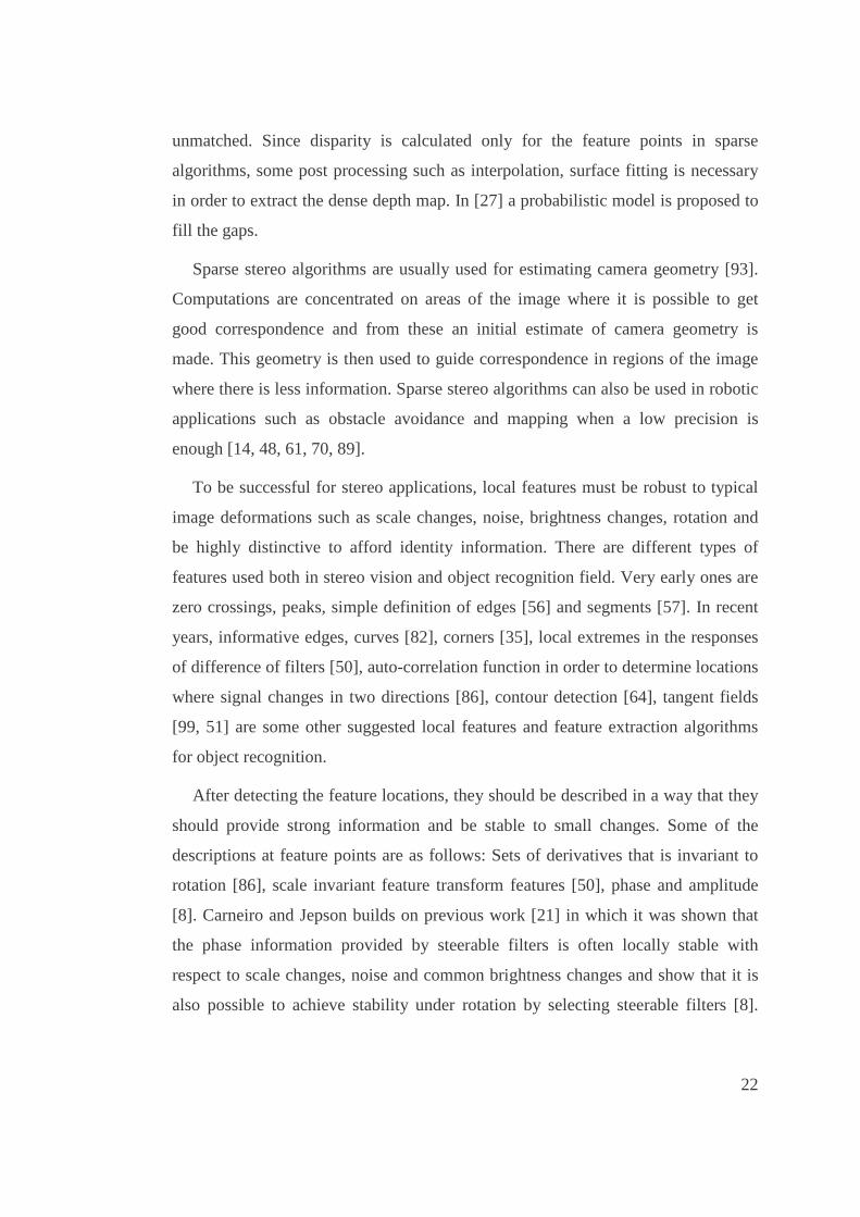
22
unmatched. Since disparity is calculated only for the feature points in sparse
algorithms, some post processing such as interpolation, surface fitting is necessary
in order to extract the dense depth map. In [27] a probabilistic model is proposed to
fill the gaps.
Sparse stereo algorithms are usually used for estimating camera geometry [93].
Computations are concentrated on areas of the image where it is possible to get
good correspondence and from these an initial estimate of camera geometry is
made. This geometry is then used to guide correspondence in regions of the image
where there is less information. Sparse stereo algorithms can also be used in robotic
applications such as obstacle avoidance and mapping when a low precision is
enough [14, 48, 61, 70, 89].
To be successful for stereo applications, local features must be robust to typical
image deformations such as scale changes, noise, brightness changes, rotation and
be highly distinctive to afford identity information. There are different types of
features used both in stereo vision and object recognition field. Very early ones are
zero crossings, peaks, simple definition of edges [56] and segments [57]. In recent
years, informative edges, curves [82], corners [35], local extremes in the responses
of difference of filters [50], auto-correlation function in order to determine locations
where signal changes in two directions [86], contour detection [64], tangent fields
[99, 51] are some other suggested local features and feature extraction algorithms
for object recognition.
After detecting the feature locations, they should be described in a way that they
should provide strong information and be stable to small changes. Some of the
descriptions at feature points are as follows: Sets of derivatives that is invariant to
rotation [86], scale invariant feature transform features [50], phase and amplitude
[8]. Carneiro and Jepson builds on previous work [21] in which it was shown that
the phase information provided by steerable filters is often locally stable with
respect to scale changes, noise and common brightness changes and show that it is
also possible to achieve stability under rotation by selecting steerable filters [8].

23
They deform a given image by changing the brightness, introducing non-uniform
brightness variation, adding noise, changing scale and rotation and select interest
points by Harris corner detector [35] on both the original and the deformed images.
Then steerable quadrature filter pairs are used to obtain local amplitude and phase
information. Since a pixel does not provide a distinctive response, they considered
M sample points taken from a region around each interest point. At each spatial
sample point (i.e. the interest point and the sample points taken from a region
around it) the filters are steered to N equally spaced orientations starting from the
main orientation of the pixel computed as described in [26]. The resulting phase-
based, complex feature vector has M*N individual components specified by the
complex filter responses. Finally, they computed the similarity between local
features between the original and the deformed images using normalized phase
correlation since this is known to provide some stability to typical image
deformations. The detection rate is defined to be the proportion of interest points
such that there are some interest points in the transformed image which is both
sufficiently close to the mapped point and which has a similar local feature vector.
They compared their results with differential invariant features [86] and showed
that phase-based feature displays consistently better results.
In order to make the phase-based approach more comparable to the other
approaches, Carneiro and Jepson also introduce a new form of multi-scale interest
point detector [9]. Since Harris corner detector is not very robust to scale changes,
they use an approach similar to [17], in which they check local spatial information
to determine whether the current scale is appropriate. They calculate the local
frequency of the response with the derivative of the phase signal and the interest
points that have local frequency close to the mean frequency of all the interest
points are selected to be locally stable. In order to achieve semi-invariance to scale
changes, space is sampled at a discrete set of scales. Given a feature vector from a
test image, they searched database for similar features, irrespective of the specific
scales at which they were observed in the test and model images. Then the specific

24
scales belonging to the matched features provide some information about the
relative scales of the target in the test and the database images. They conclude that
although phase-based local feature performs better in terms of common illumination
changes, 2D rotation and sub-pixel translation, for scale and large shear changes
both shift invariant feature transformation and the differential invariants produce
better results. However, they also suggest that the robustness of the phase-based
feature to scale changes can be improved by using a denser sampling in the scale-
space.
2.3.3 Biological Stereo Algor ithms
In many recent studies, spatial filtering of the image pairs by Gabor filters is well
accepted because Gabor filters are limited spatially and have finite bandwidth.
Another attractive aspect of using Gabor filters is their orientation selectivity. The
usage of Gabor filters is also supported by some physiological findings. A Gabor
filter has a shape very similar to the receptive field profile of simple cells in primate
visual cortex. It is also found that adjacent simple cells have the same orientation
and spatial frequency and are in quadrature pairs. This observation also leads the
researchers to think that phase of a complex Gabor filter can be internally encoded
by such a pair of neighboring simple cells.
In their experimental studies, Freeman, Ohzawa and Anzai [25, 67, 68, 1-3]
obtained monocular receptive fields and binocular interaction receptive fields for
simple and complex cells in adult cats. And they showed that these cells could be
modeled by Gabor-like functions. They also show experimentally that the receptive
fields for the left and right eye can be similar in some cells, but are clearly different
for the others and the degree of differences between receptive fields is quantified by
using receptive field phase. This observation has lead to the use of Gabor filters to
model the phase difference for the receptive fields to act as disparity decoders.
Inspired from all these findings, Anzai et. al. [1-3] models disparity selective
complex cells. In this feed forward model of disparity extraction, complex cells are
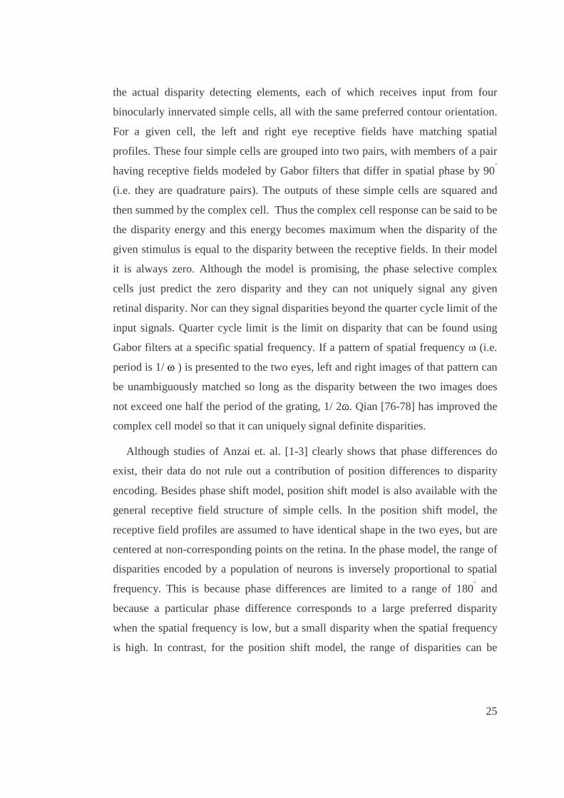
25
the actual disparity detecting elements, each of which receives input from four
binocularly innervated simple cells, all with the same preferred contour orientation.
For a given cell, the left and right eye receptive fields have matching spatial
profiles. These four simple cells are grouped into two pairs, with members of a pair
having receptive fields modeled by Gabor filters that differ in spatial phase by 90˚
(i.e. they are quadrature pairs). The outputs of these simple cells are squared and
then summed by the complex cell. Thus the complex cell response can be said to be
the disparity energy and this energy becomes maximum when the disparity of the
given stimulus is equal to the disparity between the receptive fields. In their model
it is always zero. Although the model is promising, the phase selective complex
cells just predict the zero disparity and they can not uniquely signal any given
retinal disparity. Nor can they signal disparities beyond the quarter cycle limit of the
input signals. Quarter cycle limit is the limit on disparity that can be found using
Gabor filters at a specific spatial frequency. If a pattern of spatial frequency � (i.e.
period is 1/ � ) is presented to the two eyes, left and right images of that pattern can
be unambiguously matched so long as the disparity between the two images does
not exceed one half the period of the grating, 1/ 2� . Qian [76-78] has improved the
complex cell model so that it can uniquely signal definite disparities.
Although studies of Anzai et. al. [1-3] clearly shows that phase differences do
exist, their data do not rule out a contribution of position differences to disparity
encoding. Besides phase shift model, position shift model is also available with the
general receptive field structure of simple cells. In the position shift model, the
receptive field profiles are assumed to have identical shape in the two eyes, but are
centered at non-corresponding points on the retina. In the phase model, the range of
disparities encoded by a population of neurons is inversely proportional to spatial
frequency. This is because phase differences are limited to a range of 180˚ and
because a particular phase difference corresponds to a large preferred disparity
when the spatial frequency is low, but a small disparity when the spatial frequency
is high. In contrast, for the position shift model, the range of disparities can be

26
encoded. Fleet et. al. [38-39] uses a hybrid model of disparity encoding cell which
has its receptive field profiles differ by both an overall positional shift and a phase
difference. In his model, when receptive fields are exactly the same, then the energy
neuron is sensitive to zero disparity as in Ohzawa's model. If there is only a phase
difference between receptive fields, then the energy neuron response reaches a
maximum when the disparity is equal to the intraocular phase difference divided by
the instantaneous frequency. If there is a position shift between the receptive fields,
then the cell gives the maximum response when the disparity is equal to the position
shift. In the hybrid model where receptive fields are shifted in position and also
have phase shift, the binocular energy response of the neuron depends continuously
on both the position shift and the phase shift. This hybrid model posits that the
energy should be sampled at each spatial position, with several position shifts and
with several different phase shifts. In Figure 3, three different types of disparity
encoding cell models are shown. The leftmost drawing is for position shift model
where the internal structure of the receptive fields is the same but cells are
positioned at non-corresponding points on the retina. The middle drawing is for
phase shift model where cells are positioned at corresponding points on the retina
but have phase difference. The right most drawing is for the hybrid model where
both cells are positioned at non-corresponding points and have phase difference.
Figure 3 Different models for disparity encoding cells: a. Position shift model, b. Phase
shift model, c. Hybrid model. (Picture is taken from [19])
27
Using phase difference in complex Gabor filters to decode disparity is not
limited to models of complex cells using phase differences only. But complex
Gabor filters have also been used for finding disparity from the region-based phase
differences between the left and right images [84]. Sanger filters the stereo image
pair with different oriented and sized complex Gabor filters and by checking the
regional similarities of phase of complex Gabor filtered images finds the
corresponding regions.
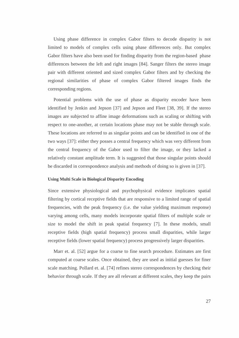
Potential problems with the use of phase as disparity encoder have been
identified by Jenkin and Jepson [37] and Jepson and Fleet [38, 39]. If the stereo
images are subjected to affine image deformations such as scaling or shifting with
respect to one-another, at certain locations phase may not be stable through scale.
These locations are referred to as singular points and can be identified in one of the
two ways [37]: either they posses a central frequency which was very different from
the central frequency of the Gabor used to filter the image, or they lacked a
relatively constant amplitude term. It is suggested that those singular points should
be discarded in correspondence analysis and methods of doing so is given in [37].
Using Multi Scale in Biological Dispar ity Encoding
Since extensive physiological and psychophysical evidence implicates spatial
filtering by cortical receptive fields that are responsive to a limited range of spatial
frequencies, with the peak frequency (i.e. the value yielding maximum response)
varying among cells, many models incorporate spatial filters of multiple scale or
size to model the shift in peak spatial frequency [7]. In these models, small
receptive fields (high spatial frequency) process small disparities, while larger
receptive fields (lower spatial frequency) process progressively larger disparities.
Marr et. al. [52] argue for a coarse to fine search procedure. Estimates are first
computed at coarse scales. Once obtained, they are used as initial guesses for finer
scale matching. Pollard et. al. [74] refines stereo correspondences by checking their
behavior through scale. If they are all relevant at different scales, they keep the pairs

28
as correct matches, otherwise they discard these matches. Inspired from the
knowledge that humans can not compare spatial phase between frequencies more
than two octaves apart, Sanger [84] combines disparities at different scales
separated by two octaves using a weighting method. In [76] a simple method which
averages over different scales is used. In [22] the energy responses at different
scales are simply summed. This pooling helps the large responses near the correct
disparity sum to produce even larger peak. Anzai et. al. [1-2] model a binocular
disparity representation in which disparity information is encoded by a group of
cells in terms of phase disparity at each size or spatial frequency scale.
2.3.4 Probabilistic stereo algor ithms
Experiences show that disparity estimations from local phase-differences as been
done in [84] are reliable near edges but yield poor results between them. In [27] a
probabilistic lattice structure is proposed to fill unreliable regions which result after
phase-based disparity estimation by using a simple smoothness constraint in the
spirit of Markov random fields. The probability of being a pair is modeled by an
exponential function (Eq 4) where the parameter is the usual local phase difference
divided by the filter wavelength, k0 (Eq 5). But in this case while the phase
difference method as used in [84] is limited to only small disparities, with the help
of exponential, longer shifts can also be considered in this case.
2),(),( RL xxdRL exxp π−= Eq 4
0
)()(),(
k
xxxxd LLRR
RL
φφ −= Eq 5
In many other probabilistic algorithms which estimate the disparity map between
the stereo images, usually the starting point is to maximize the conditional
probability of disparity given stereo images. The main problem is how to calculate
the conditional probability given only stereo image set. In [46] Gibbs’ distribution

29
is used to transform energy into probability. What is special in this study is that they
consider point wise energy based on Markov Random Fields theory where it is
proved that it is possible to estimate the disparity of a position, if all of the joint
probability distributions between neighborhood disparities are known in advance.
Assuming that the disparities in the neighborhood of a pixel are independent one
another, the joint probability can be rewritten as the product of marginal
probabilities of each disparity in the neighborhood. Myers, Wilson and Hancock
applied their graph edit distance method to uncalibrated stereo correspondence
problem where corrupted relational graphs are compared and matched [63]. In [59]
a probability distribution function for disparity gradient is proposed for windowing
operation. They formulated the relation between the maximum search space in the
second image with respect to the relative displacement of the continuous edges in
the successive scan lines of the first image. In [71] his previous work [70] on
matching edge images for robot localization is generalized. Using a probabilistic
framework, his method considers the distance from each pixel in the template to the
closest matching pixel in the image. The joint probability density function is
approximated as the product of each individual probability distribution function,
assuming that the distance measurements are independent. This study is also a good
example in order to show the close relation between stereo matching and robot
localization.
2.4 Reconstruction from Multiple Images
3D point clouds obtained by image matching are intermediate results and should be
integrated into a 3D surface model. Methods that manipulate or create surfaces in
the object space can be listed as follows:
Surface fitting to organized data points: Besides the coordinates of the points,
connectivity information is also available for each view. Usual surface fitting
algorithms can directly be applied.
30
Surface fitting to unorganized data points: Surfaces are fitted to unorganized
point cloud in the object space. A given initial mesh can be deformed by energy
minimization, planar surface patches can be fit to 3D points defined by
segmentation of color images, points can be clustered into regions of similar surface
orientation for surface fitting to unorganized data. In [29] iterative re-weighted
least-squares is used where the surface primitives are small disks in 3D called
“oriented particles” . Lelo� lu and Halici fit growing planar surfaces to 3D points
[47].
Minimizing re-projection error by optimization: The surfaces in 3D are
obtained with no need to a prior image matching phase. For the purpose of
maximization of multi-image correlation by changing parameters of a surface, in
[28] an objective function defined over multiple images is minimized by moving the
vertexes of a triangular mesh.
Volumetr ic methods: Surfaces are obtained without explicit matching. In the
space carving method, part of the space that contains objects is divided into voxels
and outermost voxels of the volume are removed if they are not justified by the
images [62]. When the volume does not shrink any more, a surface covering the
volume is generated. There is no explicit surface model until the volume is
generated.
2.5 Biological Navigation and Robotic Applications
Navigation means directing a ship to its destination. This includes three steps: 1.
The navigator determines the ship’s position on a chart as accurately as possible. 2.
On the chart, he relates his position to the destination, reference points and possible
hazards. 3. Based on this info, he sets the new course of the vessel. As a similar
approach, the steps of navigation in robotics can be listed as follows: 1. The robot
finds where it is. 2. The robot discovers where the other places are with respect to it.
3. The robot plans how to get to other places from where it is.
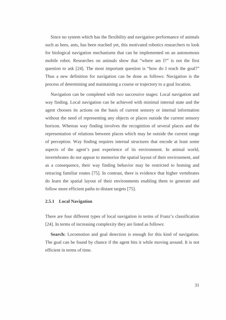
31
Since no system which has the flexibility and navigation performance of animals
such as bees, ants, has been reached yet, this motivated robotics researchers to look
for biological navigation mechanisms that can be implemented on an autonomous
mobile robot. Researches on animals show that “where am I?” is not the first
question to ask [24]. The most important question is “how do I reach the goal?”
Thus a new definition for navigation can be done as follows: Navigation is the
process of determining and maintaining a course or trajectory to a goal location.
Navigation can be completed with two successive stages: Local navigation and
way finding. Local navigation can be achieved with minimal internal state and the
agent chooses its actions on the basis of current sensory or internal information
without the need of representing any objects or places outside the current sensory
horizon. Whereas way finding involves the recognition of several places and the
representation of relations between places which may be outside the current range
of perception. Way finding requires internal structures that encode at least some
aspects of the agent’s past experience of its environment. In animal world,
invertebrates do not appear to memorize the spatial layout of their environment, and
as a consequence, their way finding behavior may be restricted to homing and
retracing familiar routes [75]. In contrast, there is evidence that higher vertebrates
do learn the spatial layout of their environments enabling them to generate and
follow more efficient paths to distant targets [75].
2.5.1 Local Navigation
There are four different types of local navigation in terms of Franz’s classification
[24]. In terms of increasing complexity they are listed as follows:
Search: Locomotion and goal detection is enough for this kind of navigation.
The goal can be found by chance if the agent hits it while moving around. It is not
efficient in terms of time.

32
Direction following: The agent must be able to align its course with a locally
available direction to find the goal. The goal does not need to be perceivable during
approach. If the agent displaced from the trail, it will miss the goal. E.g. ship setting
its course along a fixed compass direction. Inspired from flying insects which are
able to centre their flight path in a corridor by balancing image motion in their two
eyes [11], a robot equipped with a wide angle camera follows the walls in a corridor
by balancing the maximal flow on both sides and centering its course between the
nearest objects.
Aiming: An agent has to orient its body axis such that the goal is in front of it.
The goal must be perceivable during approach. E.g. ship navigating to a widely
visible light house. In [36] a robot with motion detecting camera is used in the same
manner as flies do. When an isolated object passes from front to back during flight,
the fly compensates for the optic flow created by the object by counter rotating until
the object is brought in front of the insect where it creates no image motion.
Guidance: the agent can be guided by spatial configuration of the surrounding
objects. Spatial information is the relation between the current location, goal and
current perceivable environment: E.g. A ship that tries to reach a fixed position
between several islands. In [10] bees and ants are inspired where they store a
relatively unprocessed snapshot of the surrounding panorama as seen from the goal.
A robot with omni directional camera is used where the landmarks in the view are
black regions on white background. From the difference between the image
positions in the snapshot and the current view, a movement direction was computed
to reduce the perceived difference.
2.5.2 Way Finding
Way finding can also be classified into three [24]:
Recognition tr iggered response: Starting location triggers the activation of
local navigation method leading to the goal. This can be taken as the elementary
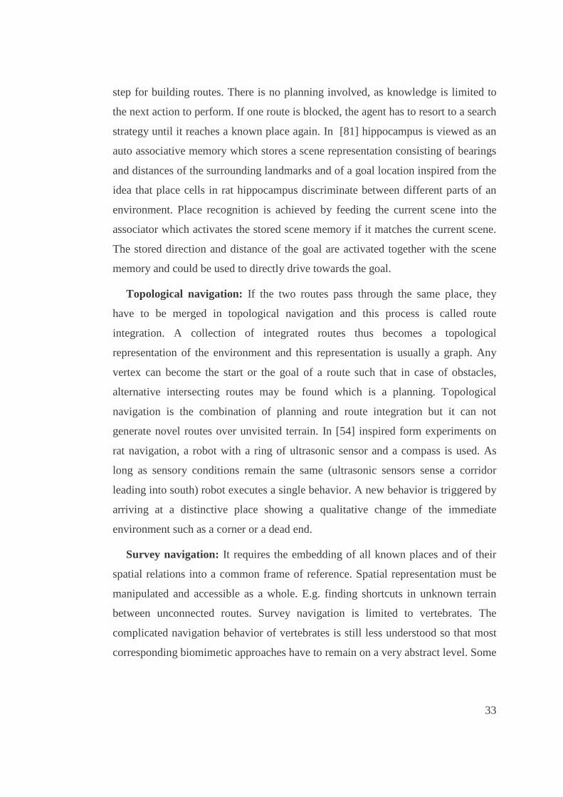
33
step for building routes. There is no planning involved, as knowledge is limited to
the next action to perform. If one route is blocked, the agent has to resort to a search
strategy until it reaches a known place again. In [81] hippocampus is viewed as an
auto associative memory which stores a scene representation consisting of bearings
and distances of the surrounding landmarks and of a goal location inspired from the
idea that place cells in rat hippocampus discriminate between different parts of an
environment. Place recognition is achieved by feeding the current scene into the
associator which activates the stored scene memory if it matches the current scene.
The stored direction and distance of the goal are activated together with the scene
memory and could be used to directly drive towards the goal.
Topological navigation: If the two routes pass through the same place, they
have to be merged in topological navigation and this process is called route
integration. A collection of integrated routes thus becomes a topological
representation of the environment and this representation is usually a graph. Any
vertex can become the start or the goal of a route such that in case of obstacles,
alternative intersecting routes may be found which is a planning. Topological
navigation is the combination of planning and route integration but it can not
generate novel routes over unvisited terrain. In [54] inspired form experiments on
rat navigation, a robot with a ring of ultrasonic sensor and a compass is used. As
long as sensory conditions remain the same (ultrasonic sensors sense a corridor
leading into south) robot executes a single behavior. A new behavior is triggered by
arriving at a distinctive place showing a qualitative change of the immediate
environment such as a corner or a dead end.
Survey navigation: It requires the embedding of all known places and of their
spatial relations into a common frame of reference. Spatial representation must be
manipulated and accessible as a whole. E.g. finding shortcuts in unknown terrain
between unconnected routes. Survey navigation is limited to vertebrates. The
complicated navigation behavior of vertebrates is still less understood so that most
corresponding biomimetic approaches have to remain on a very abstract level. Some

34
exceptions are the models of the rat hippocampus that can draw on a large number
of neurophysiological investigations where a cognitive map is thought to be stored
in the hippocampus [24]. However still there are different views for the exact role
of hippocampus in navigation. But the concept of cognitive map is highly
appreciated. Since cognitive map construction is one of the main purpose of this
thesis this subject will be investigated more in the following sub-section.
2.5.3 Cognitive Maps
Goal independent memories of spaces which are very important for topological and
survey navigation can be used for many different routes and these goal independent
memories of space are called cognitive maps. In cognitive map route description is
in this manner: “ if you want to go to B, you should turn left” . Thus cognitive maps
can be used as a route planning stage or short cut finding which are the abilities of
higher vertebrates only. Hippocampus is known to be the place for cognitive maps
and many physiological experiments have been done on rat hippocampus in order to
get more information about cognitive map structure.
In [31], starting from insect homing mechanism, higher vertebrate map
construction and shortest path discovery is modeled by neural networks. In [49]
physiological modeling of hippocampus is used for cognitive map modeling. A cell
growing ability network is constructed where different type of cells and layers of
these cells such as landmark cell layer, place cell layer are modeled. The creation of
place cell requires that at least three landmarks are nearby and visible to the agent.
Each place cell is laterally connected to some place cells neighboring to it. The
place fields of all place cells cover and partition an explored environment. As the
agent moves, it keeps track of the place where it is currently situated and the place it
previously was. Route finding is based on the traveling experience that is coded in
the weights of lateral connections between place cells. For finding the shortest path
an activation spreading process is used. In [79] a learning procedure is added on the
links of the cognitive map which enables to reinforce particular paths, and to forget
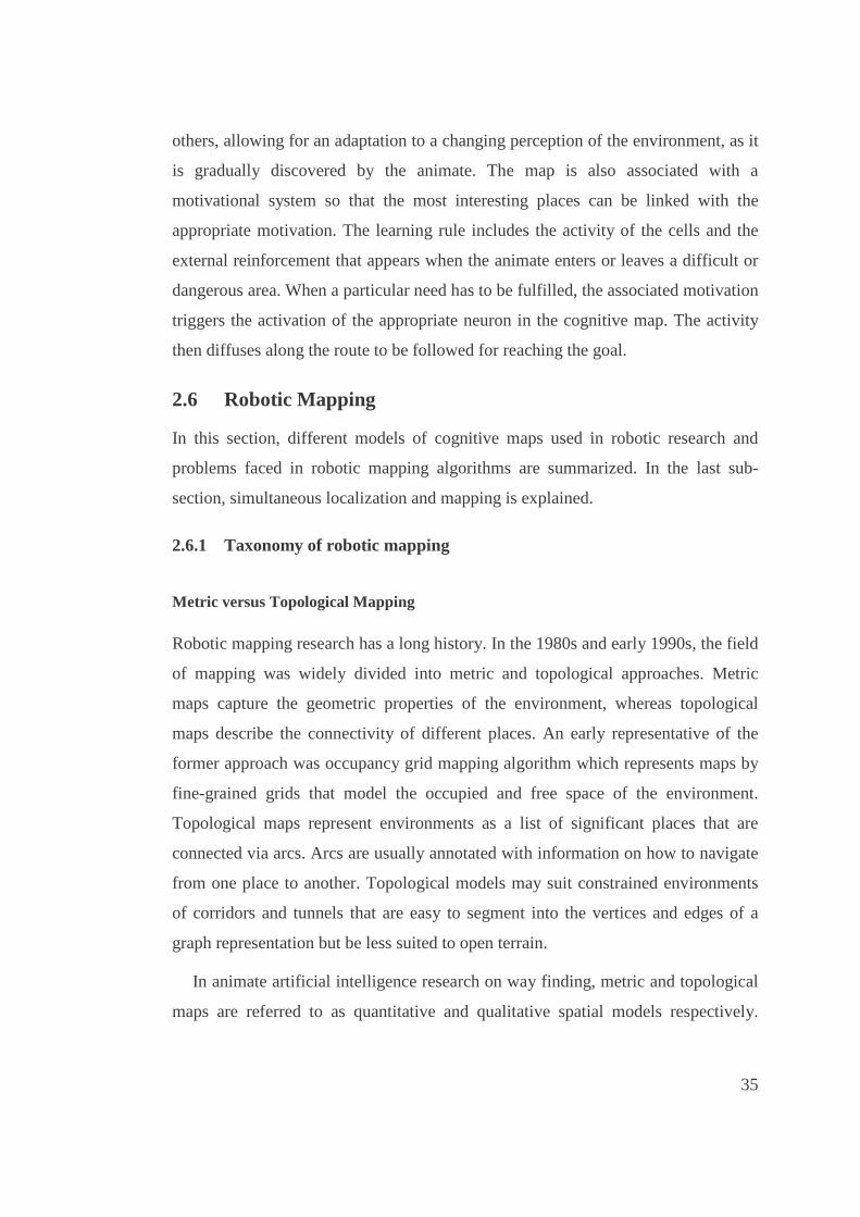
35
others, allowing for an adaptation to a changing perception of the environment, as it
is gradually discovered by the animate. The map is also associated with a
motivational system so that the most interesting places can be linked with the
appropriate motivation. The learning rule includes the activity of the cells and the
external reinforcement that appears when the animate enters or leaves a difficult or
dangerous area. When a particular need has to be fulfilled, the associated motivation
triggers the activation of the appropriate neuron in the cognitive map. The activity
then diffuses along the route to be followed for reaching the goal.
2.6 Robotic Mapping
In this section, different models of cognitive maps used in robotic research and
problems faced in robotic mapping algorithms are summarized. In the last sub-
section, simultaneous localization and mapping is explained.
2.6.1 Taxonomy of robotic mapping
Metr ic versus Topological Mapping
Robotic mapping research has a long history. In the 1980s and early 1990s, the field
of mapping was widely divided into metric and topological approaches. Metric
maps capture the geometric properties of the environment, whereas topological
maps describe the connectivity of different places. An early representative of the
former approach was occupancy grid mapping algorithm which represents maps by
fine-grained grids that model the occupied and free space of the environment.
Topological maps represent environments as a list of significant places that are
connected via arcs. Arcs are usually annotated with information on how to navigate
from one place to another. Topological models may suit constrained environments
of corridors and tunnels that are easy to segment into the vertices and edges of a
graph representation but be less suited to open terrain.
In animate artificial intelligence research on way finding, metric and topological
maps are referred to as quantitative and qualitative spatial models respectively.

36
Qualitative models of spatial layout have an important advantage over route
knowledge, in that they allow the agent to generate novel routes (using known path
segments). However, such models do not allow the determination of ‘straight-line’
routes or of short cuts that cross unexplored terrain –such skills require knowledge
of the quantitative spatial relations, direction and distance, between locations. In
view of the importance of effective way finding to autonomous agents this is a very
significant point in favor of the use of quantitative spatial knowledge.
One of the basic studies of topological mapping is Franz et. al.’s learning view
graphs [23]. In their study, view graph approach from the mazes of Schölkopf and
Mallot [88] is extended to open environments. Humans are able to navigate in
unknown environments after presentation of sequences of connected views. This
has led to the concept of a view graph. A view graph is defined as a topological
representation consisting of local views and their spatial relations. Depending on the
task, these relations can be, e.g., movement decisions connecting the views, or mere
adjacencies. Since open environments do not impose a structure on the view graph,
a set of views have to be selected and the connections between them have to be
found. In their study the vertices of the acquired view graph are panoramic views of
the environment and its edges are connections between views that can be traversed
using a visual homing procedure. Since only visual information is used here, it must
be guaranteed that the recorded views are sufficiently distinct. During exploration,
the system constantly checks whether the current view becomes similar to the
already recorded snapshots. This again is a view classifier as used for the selection
of the snapshots. In a second step, the system checks whether the detected snapshot
is not yet connected to the vertex from which the current exploration step started.
Whenever these conditions hold, the system tries to home to the snapshot. If
successful, an edge connecting the two vertices is included, and the exploration
continues from the detected snapshot. In cases where the robot gets lost or bumps
into obstacles, a non-edge is recorded between both vertices thus preventing the
failed action from being repeated. During exploration, the infrared sensors of the

37
robot are continuously checked for the presence of nearby objects. If obstacles are
detected at distances larger than 1cm, the robot tries to turn away without slowing
down. Smaller distances are interpreted as collisions causing the robot to back up
and turn away from the obstacle.
In grid-based (metric) paradigm, environments are represented by evenly spaced
grids [60]. Each grid cell may include the presence of an obstacle in the
corresponding region of the environment. If the position of a mobile robot can be
tracked accurately (however usually accumulated error exists), different positions
for which sensor measurements look alike are naturally disambiguated. Nearby
geometric places are recognized as such, even if the sensor measurements differ.
Grid based approaches suffer from complexity especially when the resolution of a
grid must be fine enough to capture every important detail of the world.
In [91] grid-based map (discrete, 2D occupancy grids) is converted to a
topological map. Each grid cell <x,y> in a map has attached a value of belief that
this cell is occupied. Belief is defined as whether or not the center of the robot can
be moved to the center of that cell. Occupancy values are determined based on
sensor readings where sonar interpretations must be integrated over time to yield a
single, consistent map. Using Bayesian approach and conditional independence
approximation, integration over time for sonar sensors are obtained. In the presence
of odometric errors maps are usually less accurate. In their study, wheel encoders,
map matching and wall orientation information are integrated in order to minimize
position error. After obtaining the grid-based map the following algorithm is
applied to convert it to a topological map: First each occupancy value in the
occupancy grid is thresholded. Then Voronoi diagram is constructed and critical
points on the Voronoi diagram, which are the points that minimize clearance
locally, are found. Critical lines are obtained by connecting each critical point with
its basis points. These critical lines partition the free-space into disjoint regions.
Finally, the partitioning is mapped into an isomorphic graph. Each region
corresponds to a node in the topological graph, and each critical line to an arc.

38
The distinction between metric and topological has always been fuzzy, since
virtually all working topological approaches rely on geometric information. In
practice, metric maps are finer grained than topological ones. Higher resolution
comes at a computational price, but it helps to solve various hard problems, such as
the correspondence.
Many quantitative navigation systems seek to construct maximally accurate
metric world models. Such an aim can justify the construction of a unified model,
into which all available observations are integrated, as the most efficient way to
minimize errors in estimates of spatial position. However, from the point of view of
a navigator, accuracy may not be the key criterion for determining the adequacy of
its spatial knowledge [75]. This is shown by recognizing that effective way finding
rarely needs an accurate assessment of the position of a remote target – a navigator
who begins with just a coarse estimate of the required heading can ‘home in’ on the
distant goal by making successive corrections based on incoming perceptual data
[75]. Rather than seeking to maximize accuracy, the animate artificial intelligence
approach emphasizes strategies for coping with the inevitable error and uncertainty
attached to acquired knowledge.
World-centr ic Versus Robot-centr ic Mapping
Historically, a second taxonomy of mapping algorithms is world-centric versus
robot-centric. World-centric maps are represented in a global coordinate space. The
entities in the map do not carry information about the sensor measurements that led
to their discovery. Robot-centric maps, in contrast, are described in measurement
space. They describe the sensor measurements a robot would receive at different
locations. At first glance, robot-centric maps might appear easier to build, since no
‘ translation’ of robot measurements into world coordinates is needed. However,
robot-centric maps suffer two disadvantages. First, it is often difficult to extrapolate
from individual measurements to measurements nearby, unexplored places –an
extrapolation that is typically straightforward in world-centric approaches. Second,

39
if different places look alike, robot-centric approaches often face difficulties to
disambiguate them, again due to the lack of an obvious geometry in measurement
space. For these reasons, the dominant approaches to date generate world-centric
maps. For example in [75], a quantitative model of environmental layout is
achieved by integrating observations from different egocentric view-points into
representations with respect to environment-centered co-ordinate frames.
2.6.2 Problems in Robotic Mapping
Sensor Problems
To acquire a map, robots must possess sensors that enable it to perceive the outside
world. Sensors commonly brought to bear for this task include cameras, range
finders using sonar, laser, and infrared technology, radar, tactile sensors, compasses,
and GPS. However, all these sensors are subject to errors, often referred to as
measurement noise. More importantly, most robot sensors are subject to strict range
limitations. For example, light and sound cannot penetrate walls. These range
limitations makes it necessary for a robot to navigate through its environment when
building a map.
The motion commands (controls) issued during environment exploration carry
important information for building maps, since they convey information about the
locations at which different sensor measurements were taken. Robot motion is also
subject to errors, and the controls alone are therefore insufficient to determine a
robot’s pose (location and orientation) relative to its environment. A key challenge
in robotic mapping arises from the nature of the measurement noise.
Modeling problems are usually relatively easy to solve if the noise in different
measurements is statistically independent. If this were the case, a robot could
simply take more and more measurements to cancel out the effects of the noise.
Unfortunately, in robotic mapping, the measurement errors are statistically
dependent. This is because errors in control accumulate over time, and they affect

40
the way future sensor measurements are interpreted. Accommodating such
systematic errors is the key to building maps successfully, and it is also a key
complicating factor in robotic mapping. Many existing mapping algorithms are
therefore surprisingly complex, both from a mathematical and from an
implementation point of view.
Size Problem
The second complicating aspect of the robot mapping problem arises from the high
number of the entities that are being mapped. A detailed two-dimensional floor
plan, which is an equally common representation of robotic maps, often requires
millions of numbers.
Correspondence Problem
A third and possibly the hardest problem in robotic mapping is the correspondence
problem also known as the data association problem. The correspondence problem
is the problem of determining if sensor measurements taken at different points in
time correspond to the same physical object in the world. The correspondence
problem is difficult, since the number of possible hypotheses can grow
exponentially over time. Although the correspondence problem was basically
ignored in the robot mapping community, in recent years it has emerged.
Dynamism Problem
Fourth, environments change over time. Some changes may be relatively slow, such
as the change of appearance of a tree across different seasons, or the structural
changes that most office buildings are subjected to over time. Others are faster, such
as the change of doors status or the location of furniture items, such as chairs. Even
faster may be the change of location of other agents in the environment, such as cars
or people. The dynamism of robot environments creates a big challenge, since it
adds yet another way in which seemingly inconsistent sensor measurements can be

41
explained. To see, imagine a robot facing a closed door that previously was
modeled as open.
There are almost no mapping algorithms that can learn meaningful maps of
dynamic environments. Instead, the predominant paradigm relies on a static world
assumption, in which the robot is the only time-variant quantity (and everything
else that moves is just noise). Consequently, most techniques are only applied in
relatively short time windows, during which the respective environments are static.
Exploration Problem
A fifth and final challenge arises from the fact that robots must choose their way
during mapping. The task of generating robot motion in the pursuit of building a
map is commonly referred to as robotic exploration. While optimal robot motion is
relatively well-understood in fully modeled environments, exploring robots have to
cope with partial and incomplete models. Hence, any viable exploration strategy has
to be able to accommodate contingencies and surprises that might arise during map
acquisition. For this reason, exploration is a challenging planning problem, which is
often solved sub-optimally via simple heuristics. When choosing where to move,
various quantities have to be traded off: the expected gain in map information, the
time and energy it takes to gain this information, the possible loss of pose
information along the way, and so on.
2.6.3 Simultaneous Localization and Mapping
Since the 1990s, the field of robot mapping has been dominated by probabilistic
techniques. A series of seminal studies introduced a powerful statistical framework
for simultaneously solving the mapping problem and the induced problem of
localizing the robot relative to its growing map. Since then, robotic mapping has
commonly been referred to as SLAM or CML, which is shortest form for
simultaneous localization and mapping, and concurrent mapping and localization
respectively.

42
Some probabilistic approaches employ Kalman filters, expectation maximization
(EM) algorithm etc. [91]. These approaches specifically address the correspondence
problem in mapping, which is the problem of determining whether sensor
measurement recorded at different points in time correspond to the same physical
entity in the real world. A third family of probabilistic techniques seek to identify
objects in the environment, which may correspond to ceilings, walls, doors that
might be open or closed, of furniture and other objects that move. Usually such
probabilistic algorithms are off-line and can not be run in real time. A real time
incremental EM in order to obtain map for cyclic environment is suggested in [92].
The mapping is formulated as a maximum likelihood estimation problem in the high
sized space of all grid maps. The estimation is carried out using the expectation
maximization algorithm. In their study the key feature is the forward modeling of
the physical sensors. Forward models describe the physics of the environment, from
causes (occupancy) to effects (measurement). In their study, the forward model is a
mixture model specific to range finders, such as sonar sensors. The optimization
begins with an entirely unoccupied map. EM then iterates two steps, an expectation
step (E step) and a maximization step (M step), thereby gradually increasing the
likelihood of the data until a local maximum is reached. The E step calculates the
expected correspondences for a given map. These expectations are simply the
probabilities for each of the possible “causes” of the sensor measurements. The M
step generates a new map for a fixed set of expectations by minimizing an energy
function. In [89], first scale invariant features are detected from the images obtained
by triclops camera system and their coordinates in 3D are found after matching
corresponding pairs. Then successive frames are matched and displacements of
these landmarks through time are found. Finally, ego-motion is calculated using
least squares minimization. Also in [14] SLAM is implemented with stereo vision
where repeatable long term localization is achieved using only naturally occurring,
automatically detected features.

43
2.7 Vir tual Environment Applications
Real robotic applications are very complicated because besides the problems of
finding how the robot should behave to complete the task at hand, the problems
faced while controlling the robot’s internal parameters brings high computational
load. The problem to be solved is not only the navigation procedure but also to
move the robot to the desired location by making the wheels turn or feet step in a
balanced way. Thus, first working in a simulated environment in order to find the
strategy to be followed by the robot and then applying this on real robot for real
applications is preferable. Thus, many studies prefer to work on simulations while
producing their algorithm. After reaching a high level of performance, the
algorithms could then be applied on real robots, of course, with necessary
modifications.
In Terzopoulos and Rabie [80,90] biologically inspired active vision system is
implemented on artificial fishes in a virtual environment. Each eye of a fish is
implemented as four coaxial virtual cameras to approximate the spatially
nonuniform, foveal/peripheral imaging capabilities typical of biological eyes. The
system consists of two modules: a foveation module and a stabilization module.
These enable the artificial fish to stabilize the visual target in its field of view,
foveate the target, and visually navigate towards the target. In Jerbic et. al. [41] the
planning of intelligent robot behavior in simulated environment is investigated.
Action plan and work space structure, are stored in a list and in a shadowed neural
network respectively. In [87] simulation of the environment and a virtual camera
taking snapshots from this environment are used to improve a real robot’s self-
localization where real camera snapshots are taken by an on-board camera. In [55]
simulation of a corridor world is constructed. A real robot is run by an operator to
obtain images. Real images are inserted into virtual corridors as texture. Then
virtual and real robots are let to move. Robots compare what they see and what they
memorized and then move accordingly. In [97], computer simulations are used to
compare exploration efficiency in a 3D field with cognitive map, without cognitive

44
map and with random exploration. In Quoy et. al. [79] a learning procedure is added
on the links of the cognitive map which enables to reinforce particular paths, and to
forget others, allowing for an adaptation to a changing perception of the
environment, as it is gradually discovered by the animate. In [69] a humanoid robot
which has stereo vision system and a 3D environment are simulated as a computer
program. The algorithm for the problem of vision based behavior consisting of local
map generation, planning and navigation is developed in simulation and then it is
applied on real robots. Image processing to obtain RGB color, depth and optical
flow are present where the robot’s duty is to find and track a red ball.

45
CHAPTER 3
BIOLOGICAL STEREO VISION WITH MULTI SCALE PHASE BASED FEATURES
3.1 Introduction and Motivation
In this part of the thesis we propose a sparse disparity algorithm. Instead of corners
which are very sparse, we prefer edges of high information as features to be
matched. We inspired from the work of Ludke and Hancock [51] in finding our
features. In their study, population coding of a bank of 8 complex Gabor filters of
different orientation is used to extract features. The orientation selective complex
cells found in a cortical hyper column are modeled by the response moduli of a
bank of complex Gabor filters. The local maximum search in order to obtain
distinctive points is performed and only points of high contrast and high certainty
“survive” . These points are usually located at object boundaries.
In our algorithm we used multi-scale phase information in order to match our
sparse features. In doing this, we inspired from the biological disparity encoding
cell models where phase is used to encode disparity. In the experimental studies of
Anzai et. al. [1, 2, 3] phase shift model of binocular cell was proposed. In their
model receptive fields of a binocular cell are at the same position in the two eyes
but have phase differences. Their study also shows that besides phase shift model,
position shift model is also available with the general receptive field structure of
simple cells. In the position shift model, the receptive field profiles are assumed to

46
have identical shape in the two eyes, but are centered at non-corresponding points
on the retina.
Using phase difference in complex Gabor filters to decode disparity is not
limited to models of complex cells using phase differences only. Jenkin and Jepson
[37-39] and Sanger [84] describe promising methods based on the output phase
behavior of band-pass Gabor filters. Fleet, Jepson and Jenkin [39] discuss further
justification for such techniques based on the stability of band-pass phase behavior
as a function of typical distortions that exist between left and right views. Recently,
Carneiro and Jenkin provide multi-scale phase-based stable features [8, 9].
Our approach is as follows: We commence from feature points detected using
steerable filtering method [26] as being done in [18]. With this method, we have
feature points with orientation information. Next, phase at different scales are
calculated and a phase vector is formed for each feature point. Then,
correspondences are estimated using the similarity of phase at multiple scales where
magnitude is used as weighting. In this way we avoid the singular points
encountered in the method of Jenkin and Jepson [38-39]. After calculating disparity
from the positional difference between corresponding points, fine-tuning in
disparity is performed using the phase difference information. We also propose a
probabilistic model for corresponding point matching. In the following sections,
extraction of features using population coding by the method of Ludke [51], our
feature extraction method using steerable filters, disparity estimation, fine tuning in
disparity, depth calculation and our probabilistic model are explained in the given
order. Also the flow chart of our stereo vision algorithm is given in Figure 2.
3.2 Feature Extraction by Population Coding Method
Gabor filters (Eqs 6,7) are well known models of orientation selective cells in striate
cortex [13]:

47
Eq 6
Eq 7
Here xσ , yσ express width of 2D Gaussian envelope along x and y direction
which can be considered the radius of the receptive field, 0ω is the spatial frequency
and θ gives the orientation in space.
Experiments show that adjacent simple cells have the same orientation and
spatial frequency, but are in quadrature pairs (i.e. they differ in spatial phase by 90o)
[15]. Thus a simple cell pair can be expressed by a complex Gabor filter which can
encode phase:
[ ]�
��
��
� �
++���
�
���
�+−= θθπω
σσθω sincos2
22exp),,,( 02
2
2
2
0 yxiyx
yxgyx
Eq 8
Although it is clear that cortical neurons are capable of responding to a diversity
of feature contrast patterns, orientations and scales, combinational models of how to
combine these responses have also proved quite elusive. Gabor filter banks provide
rather coarse estimates of feature orientation unless the full range of orientations is
sampled with a large number of filters, which is obviously highly inefficient.
Recently, however, there has been a suggestion that neuronal ensembles of the sort
encountered in cortical hyper columns can be conveniently encoded using a
population vector [32]. When population coding is used to represent the convolution
responses of the filter bank, the outputs of only a small number of filters need to be
combined in order to achieve a considerable improvement of the precision of
orientation estimation. In fact, population coding has become an essential paradigm
[ ]) sin cos ( 2 cos 2 2
exp) , , , ( 0 2
2
2
2 0 θ θ πω
σ σ θ ω y x
y x y x g
y x
+ * � � �
�
� � �
� + − =
[ ]) sin cos ( 2 sin 2 2
exp) , , , ( 0 2
2
2
2 0 θ θ πω
σ σ θ ω y x
y x y x g
y x +*
� � �
�
� � �
� +− =
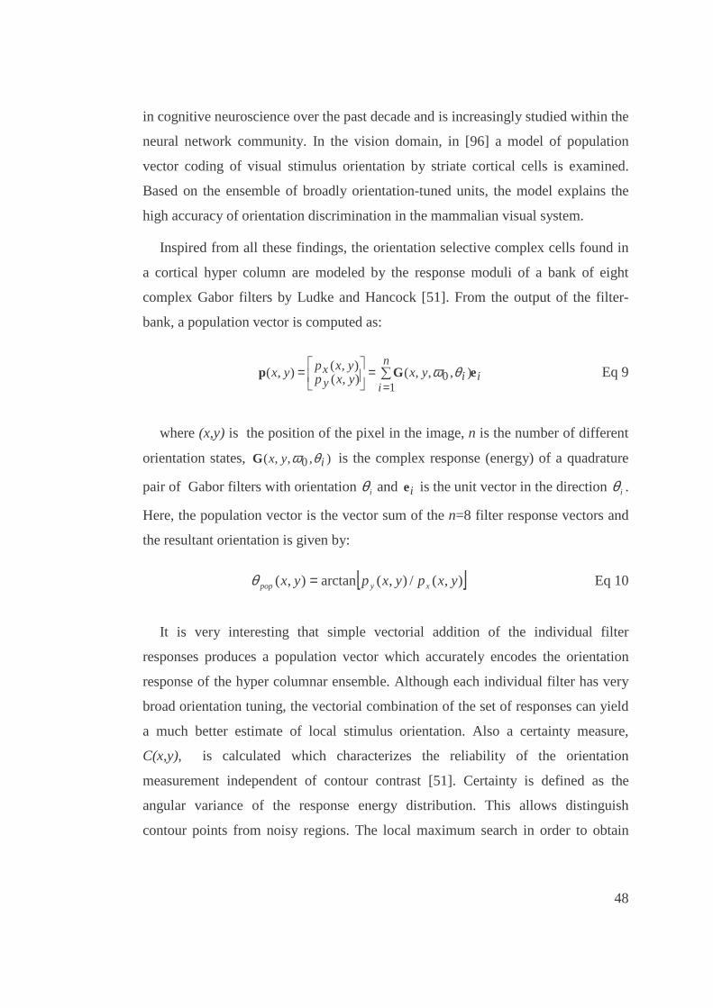
48
in cognitive neuroscience over the past decade and is increasingly studied within the
neural network community. In the vision domain, in [96] a model of population
vector coding of visual stimulus orientation by striate cortical cells is examined.
Based on the ensemble of broadly orientation-tuned units, the model explains the
high accuracy of orientation discrimination in the mammalian visual system.
Inspired from all these findings, the orientation selective complex cells found in
a cortical hyper column are modeled by the response moduli of a bank of eight
complex Gabor filters by Ludke and Hancock [51]. From the output of the filter-
bank, a population vector is computed as:
in
ii
yx yxyxp
yxpyx eGp �=
=��
���
�=1
0 ),,,(),(),(),( θω Eq 9
where (x,y) is the position of the pixel in the image, n is the number of different
orientation states, ),,,( 0 iyx θωG is the complex response (energy) of a quadrature
pair of Gabor filters with orientation iθ and ie is the unit vector in the direction iθ .
Here, the population vector is the vector sum of the n=8 filter response vectors and
the resultant orientation is given by:
[ ]),(/),(arctan),( yxpyxpyx xypop =θ Eq 10
It is very interesting that simple vectorial addition of the individual filter
responses produces a population vector which accurately encodes the orientation
response of the hyper columnar ensemble. Although each individual filter has very
broad orientation tuning, the vectorial combination of the set of responses can yield
a much better estimate of local stimulus orientation. Also a certainty measure,
C(x,y), is calculated which characterizes the reliability of the orientation
measurement independent of contour contrast [51]. Certainty is defined as the
angular variance of the response energy distribution. This allows distinguish
contour points from noisy regions. The local maximum search in order to obtain

49
distinctive points, is performed on the product of certainty and response energy,
),(),( yxCyxp . As a result only points of high contrast and high certainty
“survive” . These points are usually located on object boundaries.
In Figure 4 we show a stereo image pair and feature points obtained from these
images using the method explained above. The estimated orientation for each
feature is given in colors.
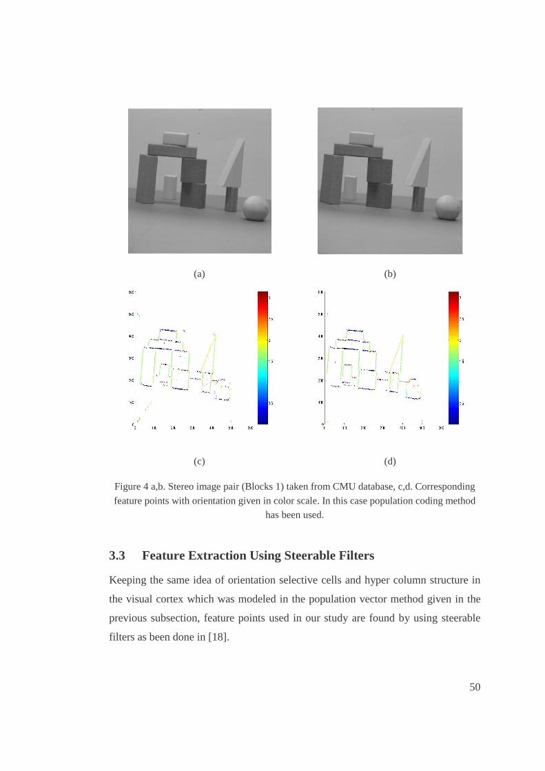
50
(a) (b)
(c) (d)
Figure 4 a,b. Stereo image pair (Blocks 1) taken from CMU database, c,d. Corresponding
feature points with orientation given in color scale. In this case population coding method has been used.
3.3 Feature Extraction Using Steerable Filters
Keeping the same idea of orientation selective cells and hyper column structure in
the visual cortex which was modeled in the population vector method given in the
previous subsection, feature points used in our study are found by using steerable
filters as been done in [18].
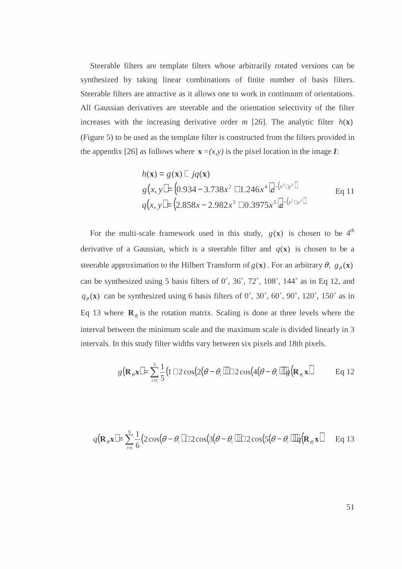
51
Steerable filters are template filters whose arbitrarily rotated versions can be
synthesized by taking linear combinations of finite number of basis filters.
Steerable filters are attractive as it allows one to work in continuum of orientations.
All Gaussian derivatives are steerable and the orientation selectivity of the filter
increases with the increasing derivative order m [26]. The analytic filter )(xh
(Figure 5) to be used as the template filter is constructed from the filters provided in
the appendix [26] as follows where x =(x,y) is the pixel location in the image I:
( ) ( ) ( )
( ) ( ) ( )22
22
53
42
3975.0982.2858.2,
246.1738.3934.0,
)()()(
yx
yx
exxxyxq
exxyxg
jqgh
+−
+−
+−=
+−=
+= xxx
Eq 11
For the multi-scale framework used in this study, )(xg is chosen to be 4th
derivative of a Gaussian, which is a steerable filter and )(xq is chosen to be a
steerable approximation to the Hilbert Transform of )(xg . For an arbitrary �, )(xθg
can be synthesized using 5 basis filters of 0˚, 36˚, 72˚, 108˚, 144˚ as in Eq 12, and
)(xθq can be synthesized using 6 basis filters of 0˚, 30˚, 60˚, 90˚, 120˚, 150˚ as in
Eq 13 where iθR is the rotation matrix. Scaling is done at three levels where the
interval between the minimum scale and the maximum scale is divided linearly in 3
intervals. In this study filter widths vary between six pixels and 18th pixels.
( ) ( )( ) ( )( )( ) ( )�=
−+−+=5
1
4cos22cos215
1
iii i
gg xRxR θθ θθθθ Eq 12
( ) ( ) ( )( ) ( )( )( ) ( )�=
−+−+−=6
1
5cos23cos2cos26
1
iiii i
qq xRxR θθ θθθθθθ Eq 13

52
(a)
(b)
Figure 5 The template filter used in analysis. a. The real part which is the 4th derivative of
Gaussian, b. The Imaginary part which is a steerable approximation to the Hilbert transform of the real part.
After defining the filters, as the first step, the image is filtered with basis filters at
three different scales and at each scale these are used to interpolate the filtered
images of orientation between 0º to 180º with 10º degrees of interval by using
equations 12 and 13. Then, the orientation estimation, )(~
xθ , is done as follows:
�=
=S
nnr
1, )(maxarg)(
~xx θ
θθ Eq 14
where )(, xθnr is the response of steerable filtering for scale n and orientation �
and S is the number of scales. At the final step, �=
S
nn
r1
~,
)(xθ is thresholded and
feature points are extracted. For the stereo pair given in Figure 4 the feature points
are obtained and shown in Figure 6 with their orientation in color.

53
(a) (b)
Figure 6 Feature points obtained by steerable filtering for the Blocks 1 stereo image pair
given in Figure 4. The orientation is given in color scale.
In population coding method [51] explained in the previous section, the images
are filtered with 8 different oriented complex Gabor filters at a predefined
wavelength. Since only one scale is considered this makes 16 times filtering.
Population vector for each pixel location is calculated by summing the 8 different
oriented complex filter responses. Also a certainty measure is calculated for each
pixel. Feature points are selected to be the local maximum of the product of
population vector magnitude and certainty.
In steerable filtering method used in our study, 5 and 6 orientations are
considered for the real and the imaginary part of the complex filter respectively. In
this case any number of scaling is allowed and this makes (5+6)*n filtering where n
is the number of scales allowed. In order to find the best representative orientation
for each pixel, filter responses are calculated for each scale for the interval between
0˚ and 180˚ with 10˚ steps using the already obtained filter responses. The
orientation of a pixel location is selected to be the orientation which gives the

54
maximum sum of responses over scales. Feature points are selected using global
thresholding over the sum of responses at the estimated orientations.
Both of these methods use very similar filters however the population vector
method [51] is single scale but the steerable filter method used in our study is multi-
scale. In order to show the importance of using multi-scale in extracting features,
we show feature points extracted using steerable filters with different number of
scales in Figure 7.

55
(a) (b)
(c) (d)
Figure 7 Feature points extracted using filters at different number of scales. a. Single scale
where width of the filter is 6 pixels, b. Single scale where width of the filter is 18 pixels, c. Three scales where filter widths are 6, 12 and 18 pixels, d. Five scales where filter widths
are 6,10,14,18,22 pixels.

56
3.4 Finding Corresponding Pairs Using Multi-scale Phase
The main attributes used in this thesis for the corresponding pair matching of
feature points are multi-scale phase and amplitude. While extracting the feature
points as explained above we also obtain orientation information for each feature
point. Using this orientation information we calculate phase at each feature point as
follows:
���
�
���
�=
))((
))((arctan
,
,
in
ini rimag
rreal
x
x
θ
θφ Eq 15
Here, the quantity iφ is the phase at feature point i, ))(( , inrreal xθ and
))(( , inrimag xθ are real and imaginary parts of the filtered image respectively where
ix is the coordinate of feature point i, n and � are the scale and orientation of the
filter applied at feature point i. We use the phase measurements for filters of
different width, i.e. different scales, to locate correspondences. We use three filters
where the width of the narrowest filter is six pixels and the largest filter is 18 pixels.
Let [ ]Ti 321 φφφ=
� be a vector of phase estimates obtained using these filters. For
each feature point at the left image, we search over a window for feature points of
similar phase vector in the right image.
We measure the similarity of phase vectors by taking the dot product of the
phase vectors (Eq 16). The candidate j which has the largest weighted phase vector
dot product with feature point i is the one that satisfies the condition. In Eq 16, • is
used for vector dot product and * is used for element by element vector product.
Weighting vector Cij (Eq 17) is constructed by using the method described in [84].
Each element nijc shows how similar the magnitudes of feature points i and j at scale
n (Eq 18). Hence, it is the confidence value of the pair i-j.

57
{ }{ })(maxargˆijji
jj C∗•= Eq 16
���
�
�
���
�
�
=3
2
1
ij
ij
ij
ij
c
c
c
C Eq 17
��
�
�
��
�
�=
|)(|
|)(|,
|)(|
|)(|min
,
,
,
,
in
jn
jn
innij r
r
r
rc
x
x
x
x
θ
θ
θ
θ Eq 18
The matching algorithm explained above is cross checked for left to right
correspondences and right to left correspondences. In this way, we may discard
occluded feature points and unsafe matches. For the stereo pair shown in Figure 4
we find correspondences for 537 out of 980 feature points in the right-hand image.
3.5 Finding Dispar ity and Depth
Once the cameras are calibrated, that is, the internal parameters of cameras like
focal length and principle point, and the camera pose (the position and orientation
of the camera in a given common coordinate system) are known, the 3D coordinate
of a point can be found, if its projections on at least two images are available.
Assuming that corresponding points are available, 3D location of the point P can
be found by finding the intersection point of the lines passing through the camera
center and the projection of P in the images. In Figure 8 the projection of point P on
left and right images are denoted by P1 and P2. The lines starting from the projection
points and passing through the camera lenses converge at point P. In this case,
cameras are assumed to be parallel thus epipolar lines are aligned and in the
horizontal direction. Epipolar lines are the intersection of the image planes with the
plane formed by the focal centers and the object point.

58
In rectified pairs, i.e. epipolarly aligned images, the difference between the
projections of the point P on the image planes is known as the disparity, � , and is
inversely proportional to the depth which is the distance of the object point to the
reference camera. In our case depth can be calculated as follows:
d=b*f/� Eq 19
where d is the depth of the point P in the space, i.e. the distance of point P from the
plane of the lenses, b is the baseline, i.e. distance between the two lenses, f is the
focal length of the lenses, i.e. the distance of the imaging plane (retina in the human
eye) to the lenses, � is the disparity of point P, i.e. the distance between the
projection of point P on two image planes.
Figure 8 Stereo camera projection system.
In this study, we also work on stereo image pairs where parallel cameras are
used. This means that the epipolar line is in the horizontal direction and the
disparity is the horizontal pixel distance between corresponding feature point
P
P1 P2
�1
�2
b �
d
f
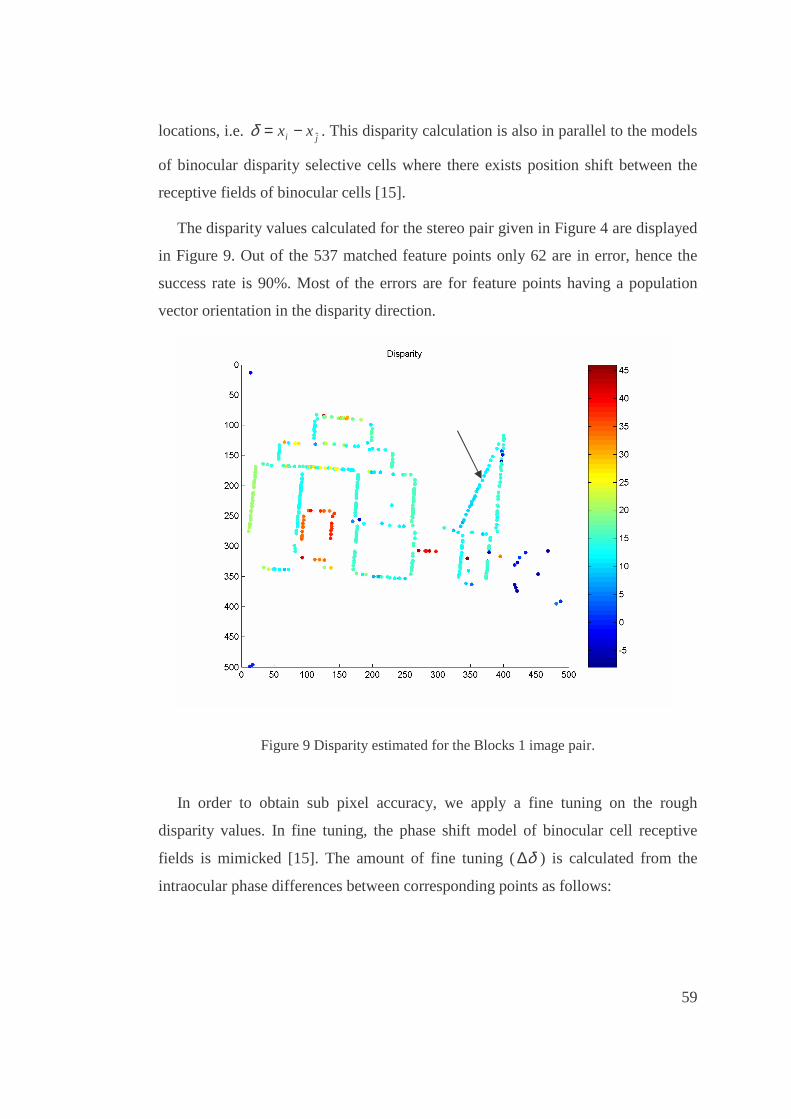
59
locations, i.e. ji xx ˆ−=δ . This disparity calculation is also in parallel to the models
of binocular disparity selective cells where there exists position shift between the
receptive fields of binocular cells [15].
The disparity values calculated for the stereo pair given in Figure 4 are displayed
in Figure 9. Out of the 537 matched feature points only 62 are in error, hence the
success rate is 90%. Most of the errors are for feature points having a population
vector orientation in the disparity direction.
Figure 9 Disparity estimated for the Blocks 1 image pair.
In order to obtain sub pixel accuracy, we apply a fine tuning on the rough
disparity values. In fine tuning, the phase shift model of binocular cell receptive
fields is mimicked [15]. The amount of fine tuning ( δ∆ ) is calculated from the
intraocular phase differences between corresponding points as follows:

60
πλφδ 2/* nnij=∆ Eq 20
Here nj
ni
nij φφφ −= is the measured phase difference at scale n between
corresponding feature points where i and j are the corresponding feature point
indenties and nλ is the wavelength used at scale n. In this way, the rough disparity
estimate expressed by integer number of pixels is tuned by the phase shift model
and sub pixel disparity, D, is calculated as follows:
δδ +∆=D Eq 21
In order to express the effect of fine tuning, the rough disparity and fine tuned
sub pixel disparity calculated on the edge-segment shown by an arrow in Figure 9
are shown in Figure 10. Here, x-axis of the plot is for the feature points on the edge
where neighboring feature points are given successive numbers starting from one
and y- axis is the disparity. The ground truth disparity changes from 13 pixels to 9
pixels on this edge. The rough disparity for each feature point is given by ‘ * ’ and
the fine tuned disparity is given by line. As can be seen on the figure, rough
disparities are in integer numbers and have a stair shaped structure whereas fine
tuned sub-pixel disparity varies smoothly.
Figure 10 Fine tuning. Feature points are numbered starting from the left-most one through
the right-most one and given in the x-axis of the plot. y-axis shows the disparity where
rough disparity is given with (* ) and fine tuned disparity given with line.

61
Disparity results for other image pairs are shown in Figures 11-14. Also, the
results are summarized in Table 1. Total number of feature points extracted from
the right image of the stereo pair, the number of pairs matched, the number of
wrong matches among matched pairs and the success rate over number of matched
pairs, i.e. the percentage of correct matches over total number of matched pairs, are
given in the successive columns of the table from left to right for each stereo pair.
Although the image pairs have very different characteristics, the results are still
satisfactory. Especially for textured locations in the images, features extracted and
multi-scale phase are very informative so that success rate is high.

62
(a) (b)
(c)
Figure 11 a. Left image, b. Right image, c. Disparity. Stereo images (Blocks 2) are taken
from CMU stereo database.

63
(a) (b)
(c)
(d)
Figure 12 a Left image, b. Right image, c. Disparity. Stereo images (Venus stereo pair) are
taken from Middlebury Stereo webpage.

64
(a) (b)
(c)
(d)
Figure 13 a. Left image, b. Right image, c. Disparity. Stereo images (Sawtooth stereo pair)
are taken from Middlebury Stereo webpage.

65
(a) (b)
(c)
(d)
Figure 14 a. Left image, b. Right image, c. Disparity. Stereo images (Tsukuba stereo pair)
are taken from Middlebury Stereo webpage.
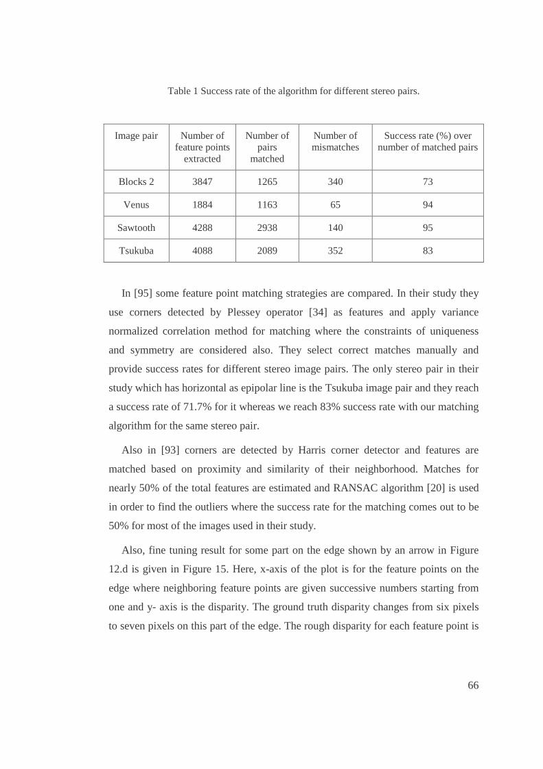
66
Table 1 Success rate of the algorithm for different stereo pairs.
Image pair Number of feature points
extracted
Number of pairs
matched
Number of mismatches
Success rate (%) over number of matched pairs
Blocks 2 3847 1265 340 73
Venus 1884 1163 65 94
Sawtooth 4288 2938 140 95
Tsukuba 4088 2089 352 83
In [95] some feature point matching strategies are compared. In their study they
use corners detected by Plessey operator [34] as features and apply variance
normalized correlation method for matching where the constraints of uniqueness
and symmetry are considered also. They select correct matches manually and
provide success rates for different stereo image pairs. The only stereo pair in their
study which has horizontal as epipolar line is the Tsukuba image pair and they reach
a success rate of 71.7% for it whereas we reach 83% success rate with our matching
algorithm for the same stereo pair.
Also in [93] corners are detected by Harris corner detector and features are
matched based on proximity and similarity of their neighborhood. Matches for
nearly 50% of the total features are estimated and RANSAC algorithm [20] is used
in order to find the outliers where the success rate for the matching comes out to be
50% for most of the images used in their study.
Also, fine tuning result for some part on the edge shown by an arrow in Figure
12.d is given in Figure 15. Here, x-axis of the plot is for the feature points on the
edge where neighboring feature points are given successive numbers starting from
one and y- axis is the disparity. The ground truth disparity changes from six pixels
to seven pixels on this part of the edge. The rough disparity for each feature point is

67
given by ‘ * ’ and the fine tuned disparity is given by line. As can be seen on the
figure, rough disparities of feature points are in integer numbers and same for all
feature points although they are slanted and should have slightly different disparity
values. Fine tuned sub-pixel disparity varies smoothly starting from just above six
pixels and extends to seven pixels.
Figure 15 Fine tuning. Feature points are numbered starting from the left-most one through
the right-most one and given in the x-axis of the plot. y-axis shows the disparity where rough disparity is given with (* ) and fine tuned disparity given with line.
In order to show the importance of using multi scale instead of single scale in
matching, we present disparity maps obtained using a single scale and three scales
in Figure 16. In both cases left to right and right to left double checking is
performed in order to get only relevant results. In the top image of Figure 16 result
given is in the case when only a single scale phase is used in matching. In the
bottom image results when multi-scale is used. Using multi-scale phase brings more
reliable results with more number of points.

68
(a)
(b)
Figure 16 Disparity calculated for Sawtooth stereo pair using: a. Single scale where filter
width is six pixels, b. Three scales where filter widths are 6, 12 and 18 pixels.
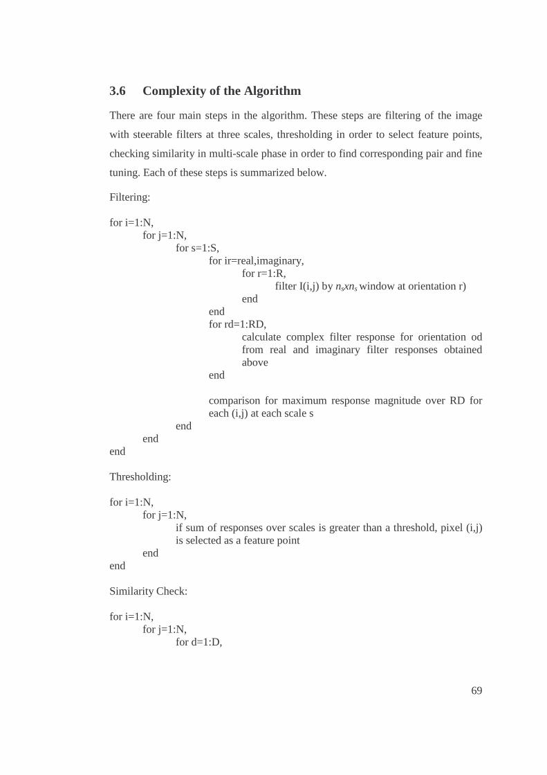
69
3.6 Complexity of the Algor ithm
There are four main steps in the algorithm. These steps are filtering of the image
with steerable filters at three scales, thresholding in order to select feature points,
checking similarity in multi-scale phase in order to find corresponding pair and fine
tuning. Each of these steps is summarized below.
Filtering:
for i=1:N, for j=1:N,
for s=1:S, for ir=real,imaginary, for r=1:R,
filter I(i,j) by nsxns window at orientation r) end
end for rd=1:RD,
calculate complex filter response for orientation od from real and imaginary filter responses obtained above
end comparison for maximum response magnitude over RD for each (i,j) at each scale s
end end
end Thresholding:
for i=1:N, for j=1:N,
if sum of responses over scales is greater than a threshold, pixel (i,j) is selected as a feature point
end end Similarity Check:
for i=1:N, for j=1:N,
for d=1:D,
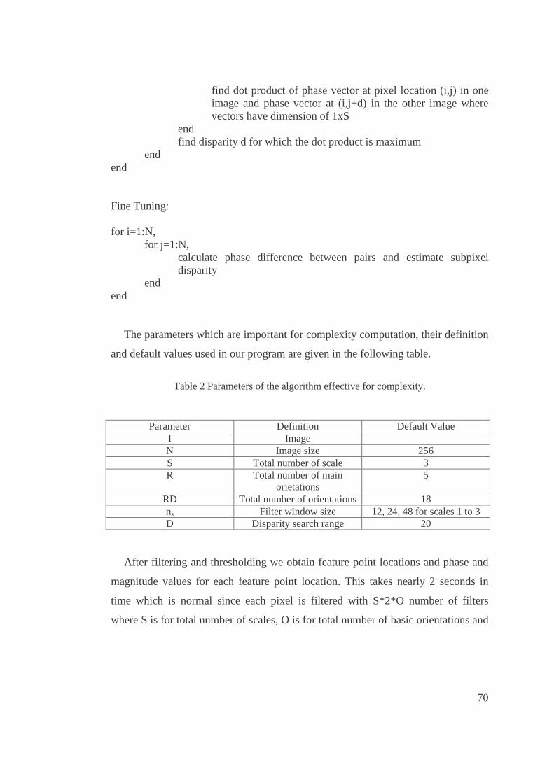
70
find dot product of phase vector at pixel location (i,j) in one image and phase vector at (i,j+d) in the other image where vectors have dimension of 1xS
end find disparity d for which the dot product is maximum
end end
Fine Tuning:
for i=1:N, for j=1:N,
calculate phase difference between pairs and estimate subpixel disparity
end end
The parameters which are important for complexity computation, their definition
and default values used in our program are given in the following table.
Table 2 Parameters of the algorithm effective for complexity.
Parameter Definition Default Value I Image N Image size 256 S Total number of scale 3 R Total number of main
orietations 5
RD Total number of orientations 18 ns Filter window size 12, 24, 48 for scales 1 to 3 D Disparity search range 20
After filtering and thresholding we obtain feature point locations and phase and
magnitude values for each feature point location. This takes nearly 2 seconds in
time which is normal since each pixel is filtered with S*2*O number of filters
where S is for total number of scales, O is for total number of basic orientations and

71
2 is for real and imaginary parts of the complex filters. The matching step is
completed in 63 milliseconds.
The complexity of the system is calculated as follows:
O ( �=
S
ssnRN
1
22 )+O ( 2N )+O ( DSN 2 )+O ( 2N ) Eq 22
where first term is for filtering step, second term is for thresholding step, third term
is for checking similarity step and last term is for the fine tuning step. For single
scale, the complexity is simplified to O( 22RnN ) and for multiple scales it comes
out to be O( 22RSnN ) where n is assumed to be the width of the widest filter.
3.7 Probabilistic Model of the Dispar ity Algor ithm
After finding correspondences and computing the associated disparities, we model
the distribution of phase differences between corresponding pairs. In order to model
a phase distribution, a circular distribution would be appropriate because of the
periodicity property of the phase. One of the circular distributions which is
appropriate for this purpose is the von Mises distribution.
The probabilistic modeling of the disparity algorithm is done as follows: First,
von Mises distribution is fit to phase differences between corresponding feature
points of Venus stereo pair. This is done once for each scale. Then, an equation for
probability of being a pair is proposed. Finally, the model is tested for its
performance on different images. Results show that although the model is based on
Venus stereo pair only, it works fine for other images such as Blocks 2, Sawtooth
and Tsukuba as well.
3.7.1 Probability Density Estimation of Phase Differences by von Mises
Model
The general form of the von Mises distribution is given by the formula:
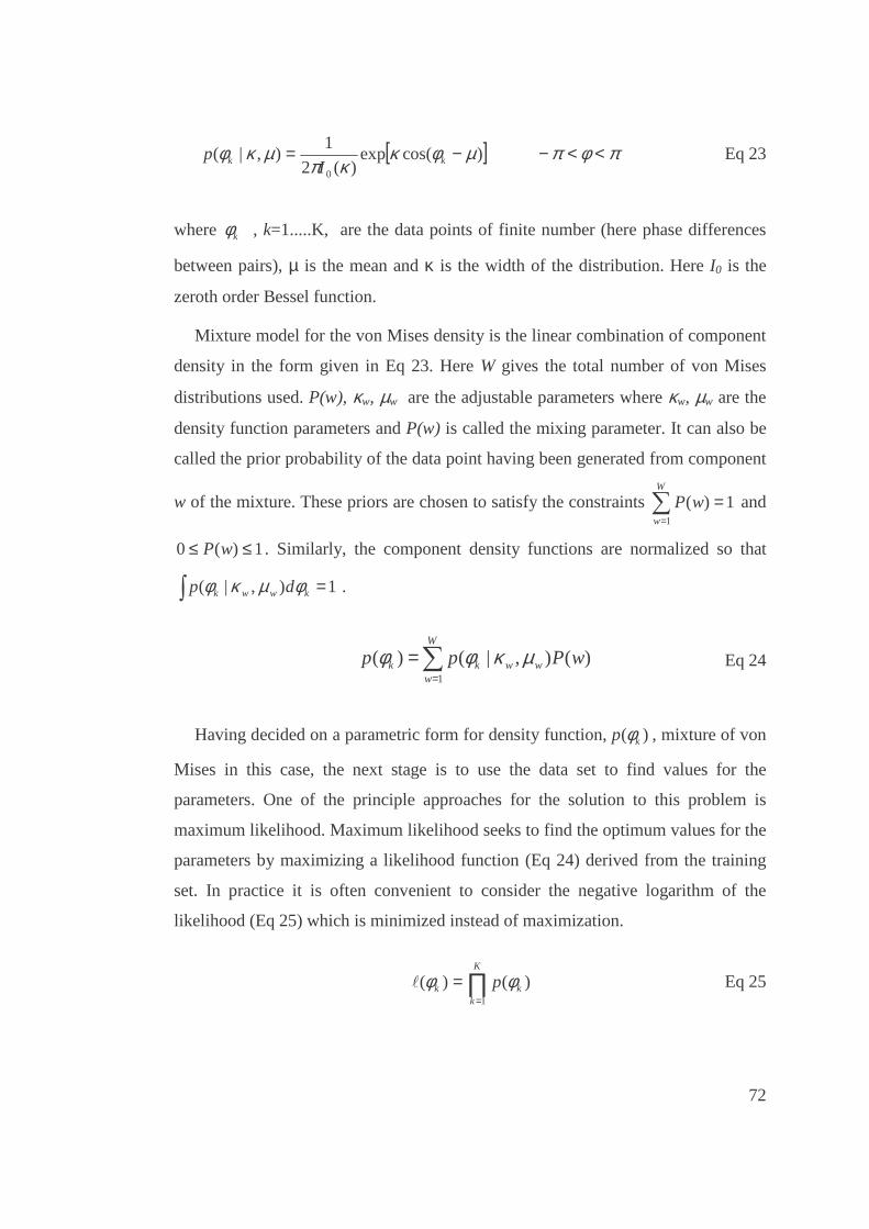
72
[ ] πφπµφκκπ
µκφ <<−−= )cos(exp)(2
1),|(
0kk I
p Eq 23
where kφ , k=1.....K, are the data points of finite number (here phase differences
between pairs), µ is the mean and κ is the width of the distribution. Here I0 is the
zeroth order Bessel function.
Mixture model for the von Mises density is the linear combination of component
density in the form given in Eq 23. Here W gives the total number of von Mises
distributions used. P(w), κw, µw are the adjustable parameters where κw, µw are the
density function parameters and P(w) is called the mixing parameter. It can also be
called the prior probability of the data point having been generated from component
w of the mixture. These priors are chosen to satisfy the constraints 1)(1
=�=
W
w
wP and
1)(0 ≤≤ wP . Similarly, the component density functions are normalized so that
1),|( =� kwwk dp φµκφ .
�=
=W
wwwkk wPpp
1
)(),|()( µκφφ Eq 24
Having decided on a parametric form for density function, )( kp φ , mixture of von
Mises in this case, the next stage is to use the data set to find values for the
parameters. One of the principle approaches for the solution to this problem is
maximum likelihood. Maximum likelihood seeks to find the optimum values for the
parameters by maximizing a likelihood function (Eq 24) derived from the training
set. In practice it is often convenient to consider the negative logarithm of the
likelihood (Eq 25) which is minimized instead of maximization.
∏=
=K
kkk p
1
)()( φφ� Eq 25

73
)(ln)(ln1
k
K
kk pE φφ �
=
−=−= � Eq 26
Using the mixture density of von Mises distribution, the log likelihood for the
data set can be given by:
� ��= ==
�
� �−=−=−=
K
k
W
wwwk
K
kkk wPppE
1 11
)(),|(ln)(ln)(ln µκφφφ� Eq 27
One of the methods to find the parameters P(w), κw, µw is to take the derivative
of E with respect to the parameter and solve by equalizing the result to zero. This
way a direct method to calculate the parameters can not be provided. In fact highly
non-linear coupled equations are represented. Thus, an iterative scheme would be
better for finding the minimum of E. An iterative scheme could be as follows: First
initial guesses for the parameters are made which are called ‘old’ values. Then the
right hand sides of the derivatives explained above are solved and this gives a
revised estimate for the parameters and these revised parameters are called as
‘new’ . These parameter values are then become the ‘old’ values and the process is
repeated. This way at each iteration the error function decreases until a local
minimum is found. This is also a special case of a more general procedure known as
the expectation-maximization (EM) algorithm.
The change in error when we replace the old parameter values by the new values
can be written as in Eq 27 where )( knewp φ denotes the probability density evaluated
using the new values for the parameters while )( koldp φ represents the density
evaluated using the old parameter values.
��
� �
−=−k k
old
knew
oldnew
p
pEE
)(
)(ln
φφ
Eq 28

74
Using the definition of mixture distribution given by Eq 23 it can be re-written as
follows [6]:
��
�
�
�
��
�
�
−=−k k
oldk
old
kold
wk
newnew
oldnew
wP
wP
p
wpwPEE
)(
)(
)(
)()(ln
φφ
φ
φ Eq 29
where )|( wp kφ is used instead of ),|( wwkp µκφ and )|( kwP φ is used instead
of )|,( kwwP φµκ for simplicity and the last term is simply the identity. Making use
of the Jensen’s equality [6] the equation becomes:
���
� �
−≤−w k
oldk
old
knewnew
kold
k
oldnew
wPp
wpwPwPEE
)|()(
)|()(ln)(
φφφ
φ Eq 30
We wish to minimize newE with respect to the ‘new’ parameters. If we let Q be
the right hand side in Eq 29 then we have QEE oldnew +≤ and so QE old +
represents an upper bound on the value of newE . Thus minimizing Q will
necessarily lead to a decrease in the value of the newE unless newE is already at a
local minimum. If we drop the terms which depend on the ‘old’ parameters, Q is
rephrased as follows where ‘n’ is used instead of ‘old’ and ‘n+1’ is used instead of
‘new’ in order to emphasize the iterative process:
{ }��= =
++++ −=K
k
W
w
nnw
nwkk
nn wPpwPQ1 1
)1()1()1()()1( )(),|(ln)|(~ µκφφ Eq 31
This function can be minimized with respect to the ‘new’ parameters at iteration
‘n+1’ . For )1(,)1( ++ nw
nw µκ this minimization is straight forward. The derivative of
the function with respect to the parameter will be equalized to zero and the result
will be solved for the parameter.

75
The update equation for )1( +nwµ is given in Eq 31. The solution is straight
forward if the posterior probabilities and the Bayes’ theorem (Eq 32, 33) are
inserted in Eq 31 then Eq 31 becomes as in Eq 34. The posterior probabilities also
satisfy 1)|(1
=�=
W
wkwP φ .
����
�
�
����
�
�
=�
�+
K
kkk
n
K
kkk
n
nw
wP
wP
)2cos()|(
)2sin()|(arctan2/1
)(
)(
)1(
φφ
φφµ Eq 32
�=
=W
wwwkk wPpp
1
)(),|()( µκφφ Eq 33
)(
)(),|()|(
k
wwkk p
wPpwP
φµκφφ = Eq 34
�������
�
�
�������
�
�
=
��
��
=
=+
K
kkW
w
nnnwk
nnnwk
K
kkW
w
nnnwk
nnnwk
nw
wPp
wPp
wPp
wPp
w
w
w
w
)2cos()(),|(
)(),|(
)2sin()(),|(
)(),|(
arctan2/1
1
1)1(
φµκφ
µκφ
φµκφ
µκφ
µ Eq 35
For )1( +nwκ the solution is not obtained directly but the R value is obtained as in
Eq 35. For the solution of R, which is a value in the range [0-1], the posterior
probabilities which are expressed using Bayes’ theorem as explained just above are
also used.
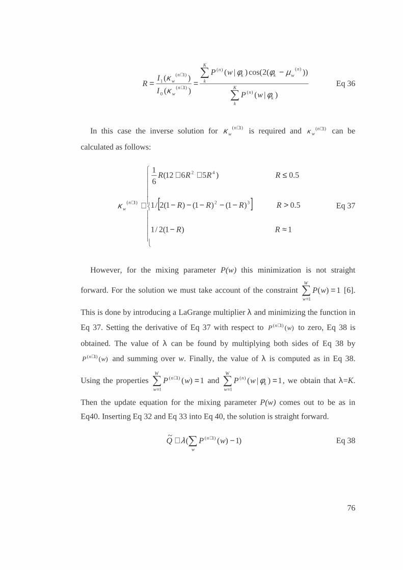
76
�
� −== +
+
K
kk
n
K
k
nwkk
n
nw
nw
wP
wP
I
IR
)|(
))(2cos()|(
)(
)(
)(
)()(
)1(0
)1(1
φ
µφφ
κκ
Eq 36
In this case the inverse solution for )1( +nwκ is required and )1( +n
wκ can be
calculated as follows:
[ ]
����
�
����
�
≈−
>−−−−−
≤++
≅+
1)1(2/1
5.0)1()1()1(2/1
5.0)5612(6
1
32
42
)1(
RR
RRRR
RRRR
nwκ Eq 37
However, for the mixing parameter P(w) this minimization is not straight
forward. For the solution we must take account of the constraint 1)(1
=�=
W
w
wP [6].
This is done by introducing a LaGrange multiplier λ and minimizing the function in
Eq 37. Setting the derivative of Eq 37 with respect to )()1( wP n+ to zero, Eq 38 is
obtained. The value of λ can be found by multiplying both sides of Eq 38 by
)()1( wP n+ and summing over w. Finally, the value of λ is computed as in Eq 38.
Using the properties 1)(1
)1( =�=
+W
w
n wP and 1)|(1
)( =�=
W
wk
n wP φ , we obtain that λ=K.
Then the update equation for the mixing parameter P(w) comes out to be as in
Eq40. Inserting Eq 32 and Eq 33 into Eq 40, the solution is straight forward.
)1)((~ )1( −+ � +
w
n wPQ λ Eq 38

77
0)(
)|(
1)1(
)(
=+−�=
+
K
kn
kn
wP
wP λφ Eq 39
�=
+=K
kn
kn
wP
wP
1)1(
)(
)(
)|( φλ Eq 40
�=+
kk
nn wPK
wP )|(1
)( )()1( φ Eq 41
The results of fitting the von Mises mixture model to phase differences between
Venus corresponding pairs at different scales are shown in Figure 17. In this case, J
is taken to be five, i.e. total number of mixed von Mises distribution components is
five. The five different components for each scale are given at the leftmost column
of the figure (Figure 17 a,c,e). As can be seen on the plots, most components are
exactly the same, thus J=5 is more than enough. On the rightmost column, the final
mixture models are shown on top of the phase difference histograms. Here, top row
(Figure 17 a,b) is for scale one, i.e. when filter of width six pixels is used, middle
row (Figure 17 c,d) is for scale two, i.e. when filter of width 12 pixels is used and
the last row (Figure 17 e,f) is for scale three, i.e. when filter of width 18 pixels is
used.

78
(a) (b)
(c) (d)
(e) (f)
Figure 17 Mixture of von Mises models for the correct pair phase differences. a, c, e.
Components of the mixture model for scale 1, 2 and 3 respectively, b, d, f. Mixture model and histogram of phase differences for scale 1, 2 and 3 respectively.

79
3.7.2 Probability of Being a Pair
With the parameters of the mixture model to hand, we can estimate correspondence
probabilities from the phase differences. The correspondence probabilities are taken
to be a posteriori probability of the mixture with the smallest mean at convergence
of the EM algorithm. Suppose that Eq 41 is the a posteriori correspondence
probability for scale n where j is the index for candidate corresponding feature
points for feature point i. The overall correspondence probability is the product of
correspondence probabilities computed at the different scales as in Eq 42 assuming
that they are independent. The correspondences are taken so as to maximize P(i=j)
as in Eq 43. Applying the correspondences located in this way the computed
disparities for Venus stereo pair are very similar to those found using the method
described in Section 3.5. Both results are shown in Figure 18.
�=j
ijn
ijn
ijn ppP )(/)()( φφφ Eq 42
∏==n
ijnPjiP )()( φ Eq 43
)(maxargˆ jiPjj
== Eq 44

80
(a)
(b)
Figure 18 Results for Venus stereo pair. a. Disparity found by the method in Section 3.5, b.
Disparity found by the probabilistic model described in Section 3.6.
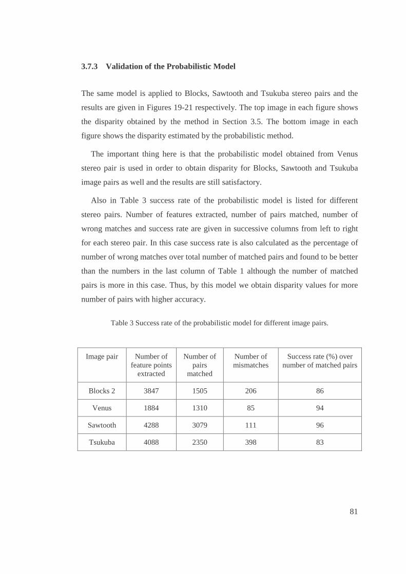
81
3.7.3 Validation of the Probabilistic Model
The same model is applied to Blocks, Sawtooth and Tsukuba stereo pairs and the
results are given in Figures 19-21 respectively. The top image in each figure shows
the disparity obtained by the method in Section 3.5. The bottom image in each
figure shows the disparity estimated by the probabilistic method.
The important thing here is that the probabilistic model obtained from Venus
stereo pair is used in order to obtain disparity for Blocks, Sawtooth and Tsukuba
image pairs as well and the results are still satisfactory.
Also in Table 3 success rate of the probabilistic model is listed for different
stereo pairs. Number of features extracted, number of pairs matched, number of
wrong matches and success rate are given in successive columns from left to right
for each stereo pair. In this case success rate is also calculated as the percentage of
number of wrong matches over total number of matched pairs and found to be better
than the numbers in the last column of Table 1 although the number of matched
pairs is more in this case. Thus, by this model we obtain disparity values for more
number of pairs with higher accuracy.
Table 3 Success rate of the probabilistic model for different image pairs.
Image pair Number of feature points
extracted
Number of pairs
matched
Number of mismatches
Success rate (%) over number of matched pairs
Blocks 2 3847 1505 206 86
Venus 1884 1310 85 94
Sawtooth 4288 3079 111 96
Tsukuba 4088 2350 398 83

82
(a)
(b)
Figure 19 Results for Block stereo pair. a. Disparity found by the method in Section 3.5, b.
Disparity found by the probabilistic model described in Section 3.6.

83
(a)
(b)
Figure 20 Results for Sawtooth stereo pair. a. Disparity found by the method in Section 3.5,
b. Disparity found by the probabilistic model described in Section 3.6.

84
(a)
(b)
Figure 21 Results for Tsukuba stereo pair. a. Disparity found by the method in Section 3.5,
b. Disparity found by the probabilistic model described in Section 3.6.
85
3.8 Summary and Conclusion
We have presented a stereo correspondence method which is motivated by
biological information. We have modeled hyper column structure of the human
visual cortex using steerable filters. Thus, instead of calculating disparities using
oriented filters and pooling the results over different orientations, a single
orientation for each feature is obtained prior to disparity computation. The steerable
filter estimate of stimulus orientation found using this method is very accurate
given the small number of filters used.
By using multi-scale filtering highly informative feature points are extracted
even they are at different scales. The use of multiple scales is also biologically
plausible. The reason for this is that disparity encoding binocular cells are sensitive
to different spatial wavelengths. Although feature points extracted from image pairs
are sparse, since they are the points of high contrast edges that define the bounding
contours of objects, they still prove to be informative.
Correspondences between feature points are located using multi-scale phase
information. This idea is also biologically grounded. The reason for this is that
simple binocular cells occur in pairs that are in quadrature phase. Also, phase is
sensitive to spatial differences, and hence it provides fine image detail which is
helpful in discriminating neighboring image regions. Phase is also robust to small
scale differences. Unfortunately, there are image locations where phase is singular
and can not be reliably used. Such points are the locations where local frequencies
at these points are very different from the filter tuning. In this study, by performing
phase comparisons at multiple scales and by using magnitude confidence
information we overcome these difficulties. The confidence weighting is used to
augment phase information with information concerning the magnitude of the
steerable filtered image to improve the correspondence method.
Two routes to locating feature-point correspondences are explored. Using the
position shift model, rough disparity values are obtained and a large range of

86
disparities can be calculated, but to a limited accuracy. Using the phase shift model,
fine tuning is performed without encountering the quarter cycle limit. This tuning
scheme also allows a continuum of disparity estimates to be obtained. Success rate
for correct matches over total number of matches is quite high when compared to
other studies in which similar type of stereo image pairs are considered. The
smallest success rate is obtained for Blocks 2 stereo pair because nearly half of the
total number of edges has orientation parallel to the epipolar line and due to the lack
of texture, phase contents are very similar for neighboring edges. The next better
success rate is for Tsukuba stereo pair. Tsukuba images are known to be a hard
image pair for stereo algorithms because they have very complicated depth
discontinuities and repeated patterns. The best success rate is obtained for Venus
and Sawtooth stereo pairs. In these pairs both textured and textureless regions exist.
Also slanted surfaces are present. Thus, they are good examples for matching
algorithms.
The complexity of our algorithm is calculated as O( 22SRnN ) where n is
assumed to be the width of the widest filter, S is the total number of scales used and
N is the image size where image is though to be square in size. The feature
extraction step of our algorithm takes time where as matching and extraction of
depth filed is real time. Although highly informative edges are selected as features
by using multi-scale strategy, it is time consuming to filter the image pair with
filters of various widths. However, with the recent development in hardware and
software and with some parallel processing we are hoping to obtain our features in
real time in the very near future.
There are of course some problems occur because of using phase in matching
since this algorithm gives results for textured regions and edges only. For texture-
less regions since there are no edges and features, no disparity value can be found.
Thus some post processing such as surface fitting is needed in order to obtain dense
disparity values.

87
There are some taxonomy papers for feature based matching however they are
dated very late. One of the recent matching algorithms is given by [93] where
feature matching is done for the purpose of camera calibration. Their feature points
are corners and proximity and similarity of feature point intensity neighborhood are
used for matching. Then RANSAC is used for computing homography. Finally
matching is guided by the estimated homography. In their study, the average
success rate over different image pairs is %50. The most recent taxonomy study for
feature matching is performed by Vincent and Laganiere [95]. They followed the
same steps as [93]. But they used variance normalized correlation between feature
points for matching. In their study Tsukuba image pair is also used in order to show
the results and they reach %67.8 success rate. Than they do left to right and right to
left symmetry check and increase their success rate to %71.7 with the number of
good matches being 195. When we apply our matching algorithm to the same
Tsukuba image pair, although the number of feature points are high in our case, we
reach a success rate of %83.
In this part of the thesis, a probabilistic algorithm for correspondence matching is
also proposed. Mixture of von Mises distributions are used to model probabilistic
matching algorithm using phase differences obtained for a stereo image pair and the
model is verified on other stereo pairs. The model provides not only better results
especially for Block 2 stereo pair but also flexibility in search region in matching.
The important thing here is that although modeling is done by Venus stereo pair
data only, it works fine for many other images. Another important thing is that von
Mises being a circular distribution has been used in EM algorithm for the first time.

88
CHAPTER 4
APPLICATION OF OUR ACTIVE STEREO VISION ALGORITHM ON A VIRTUAL ROBOT FOR
COGNITIVE MAP FORMATION AND OBJECT RECOGNITION IN A VIRTUAL ENVIRONMENT
4.1 Introduction
In the previous chapter, we explained our disparity algorithm which is based on
human vision. In this chapter we will apply it on a virtual robot for the purpose of
environmental map construction. Our disparity algorithm is a sparse algorithm and
is appropriate for such an application.
The reason why we select such an application is that we want to use our method
in a navigation activity which is achieved by humans. Humans can manage a high
level of navigation which is called survey navigation by constructing an
environmental map in the hippocampus region of the brain. The task of generating
robot motion in the pursuit of building a map is commonly referred to as robotic
exploration. While optimal robot motion is relatively well-understood in fully
modeled environments, exploring robots have to cope with partial and incomplete
models. Hence, any viable exploration strategy has to be able to accommodate
contingencies and surprises that might arise during map acquisition. For this reason,
exploration is a challenging planning problem, which is often solved sub-optimally
via simple heuristics. In this study, we also suggest a heuristic for environmental
map construction strategy using our disparity algorithm only.
89
Humans can perform many different activities simultaneously. While they are
walking, they can recognize objects that they observe around their pathways. Thus a
vision model should be such that it could be used for as many purposes as possible
such as obstacle avoidance, map construction and object recognition . The best way
of doing this is to construct a vision model which is as close to the human visual
system as possible. Our model is also good for other visual activities such as
obstacle avoidance and object recognition as well as environmental map
construction. In this chapter we also give a recognition algorithm for simple shaped
objects.
We apply our algorithm in a 3D virtual environment. There is a virtual agent in
this environment and this agent has stereo cameras which are modeled based on
human eye properties. The cameras are positioned at a height above the ground
level with six cm distance between each other just as the eyes of humans. The
cameras are controlled in the way human eyes can be. Given a target location, both
eyes look at the same target point with similar parameters such as focal length.
There are also 3D objects from the set { apple tree, pine tree, cottage} with different
shapes, sizes, textures and colors in this virtual world. These 3D objects are made
up of two basic shapes from the set { sphere, ellipsoid, cylinder, cone} . For
example, a big radius cone on top of a big radius cylinder is a cottage, whereas a
small radius cone on top of a small radius cylinder is a pine tree. Also, a sphere on
top of a cylinder is for an apple tree. The objects can be placed anywhere on the
ground in the virtual world and the agent can move anywhere around them.
We explained our physiological model of disparity extraction in the previous
chapter. For each stereo image pair that the agent obtains from the virtual
environment, disparity is extracted and depth for the current view is calculated. In
doing this we assume that the camera parameters are known by the agent just like
the eye parameters such as focal length are known by the humans. When looking at
a distant location the eye muscles activate such that the view is as clear as possible
and this is coordinated between the visual cortex and eye muscles which is

90
obviously showing that human brain is aware of the eye parameters for depth
calculation.
The map is constructed using the location information extracted from the current
view in a way that each grid value is increased by one if something is observed at
the location covered by that grid. This means that the belief of that grid being
occupied is as large as the value of that grid. Also, color information is kept for
each grid. In this study we used world centered, grid based cognitive map structure
due to its applicability, differentiability, simplicity and fine grained structure.
World-centric maps are represented in a global coordinate space. Since
disambiguation of similar but different places is hard and extrapolation from
individual measurements to measurements nearby is very difficult for robot-centric
approaches, dominant approaches to date generate world-centric maps. Occupancy
grid map is a metric map that represents the environment by fine grained grids and
models the occupied and free space of the environment whereas topological maps
only give the relative position of the things in the environment. Since metric maps
are finer grained than topological ones, places that look alike can be disambiguated
more easily. Although this high resolution comes at a computational price, it helps
to solve various hard problems. In this study, unlike the common 2D grid-based
maps, we construct 3D map of the environment.
While the agent is exploring the environment, new objects seen around are
investigated in detail. Using the location and color information, the shape of the
object parts are estimated and the whole object is classified to be either one from
the set: { apple tree, pine tree, cottage} .
Further details for virtual world construction software, map construction
algorithm and object recognition are given in the following sections.

91
4.2 Design and Implementation Details of the Simulation Software
The simulation software is developed using C++ programming language and
OpenGL graphics library on the Microsoft (MS) Windows operating system (OS)
[94]. As the user interface of the software is depicted in Figure 22, it is composed of
four panes showing the scene from different view points. The two panes above are
views from the left camera (eye) and right camera, respectively. The bottom panes
render the scene from the top viewpoint, and front viewpoint. Below of the bottom
panes, there are tab based (so called) dialog boxes which allow entering/adjustment
of the parameters used throughout algorithm implementations.
A multi-purpose user interface for displaying the calculated feature point
information is shown in Figure 23. You can either see only the rendered stereo
images or both stereo images and extracted feature points simultaneously by
selecting “Show Feature Point” option button shown under each image. By
selecting a channel from the pull-down menu called “Channel” various kinds of
information can be seen for each feature point on the screen. For example, in this
specific study, Channel 0 to Channel 2 are used to keep world coordinates of the
feature points, i.e. x,y,z locations respectively. Channel 3 is used for disparity and
Channel 4 is for agent centered depth. Any information can be arranged to be
printed on the screen with minor changes in the software. Moreover, by clicking on
a feature point by mouse, all the information about that feature point, i.e.
information of all channels, is seen in the dialog box called “Point Info” . In Figure
23, the image shown on the left side is the left camera view and the black dots on
the image show feature point locations for this current view. The image on the right
side is the right camera view and Channel 3 is selected to be shown on the feature
points thus the disparity values for the right feature points are shown in colors.
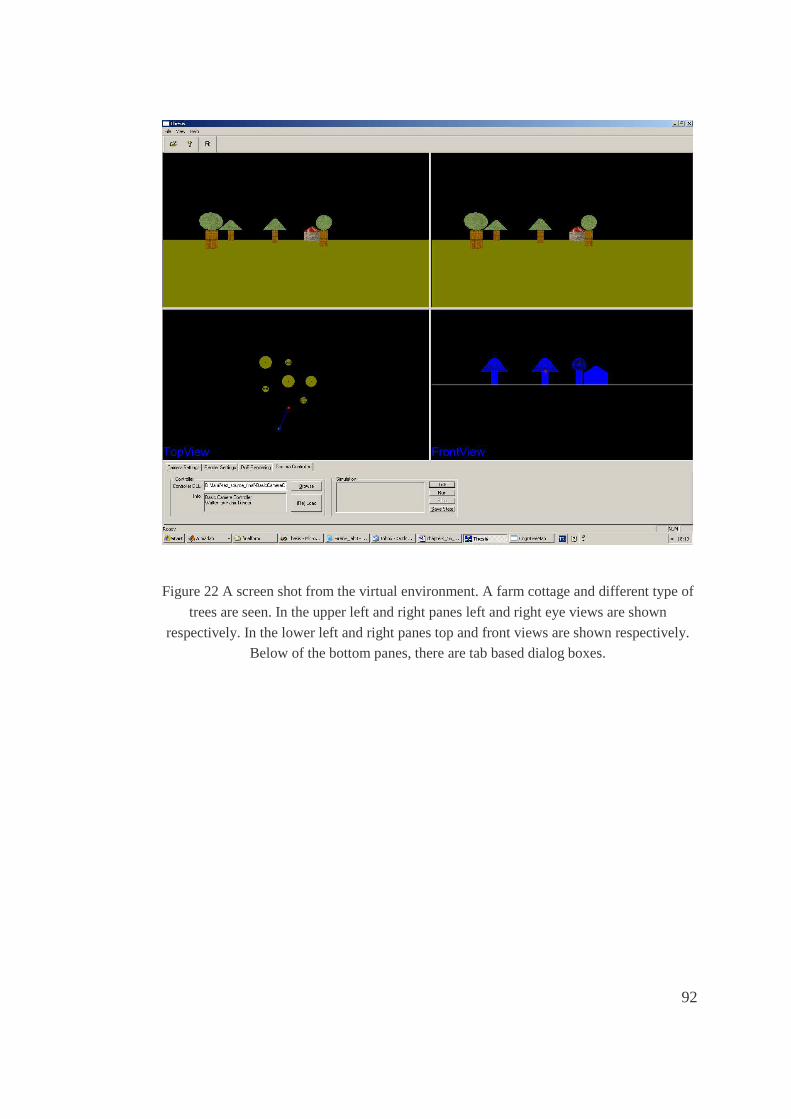
92
Figure 22 A screen shot from the virtual environment. A farm cottage and different type of
trees are seen. In the upper left and right panes left and right eye views are shown
respectively. In the lower left and right panes top and front views are shown respectively. Below of the bottom panes, there are tab based dialog boxes.

93
Figure 23 Interface for displaying feature point information. Locations of feature points for
the cottage are shown on the left camera view as black dots and disparities found are shown on the right camera view in colors.
Basically, the software should fulfill the following requirements in order to be
used in our study:
1. It should allow specifying and rendering arbitrary geometric shapes and
these shapes should be placed somewhere in the virtual environment.
2. We should locate the agent at any point on the ground of our virtual world.
3. Images rendered for the current snapshots viewed by the camera(s) (left and
right) should be exported to a specified image file for future processing.
4. We should modify the camera parameters whenever we would like. Those
modifications should be observed at interactive frame.

94
5. The software should support some kind of plug-in mechanism to be loaded
(and linked) dynamically into the application at run-time. This plug-in should
access internal structure of the scene data and image(s) rendered, so that this plug-in
would control the navigation in the scene by locating the camera. The method or
methods used by this plug-in(s) to navigate through the scene is up to the internals
and goals of the plug-in. In this study, the navigation algorithm for the purpose of
environmental map formation and object recognition will be the camera controller
plug-in.
Some assumptions made in this study are as follows:
1. Objects in the environment are made up of two parts and these parts have
one of the following basic shapes: { sphere, ellipsoid, cylinder, cone} . The shapes
can be of any size, color and texture. The final objects are either one from the set
{ apple tree, pine tree, cottage} .
2. The objects constructed from these basic shapes can be located anywhere in
the world.
3. The objects are clearly separable.
4. The agent is aware of its initial position in the world and initial orientation
with respect to global north.
5. The agent is aware of its internal camera parameters.
6. The agent is aware of its external camera parameters such as position and
gaze direction.
7. The cameras can see up to a predefined distance.
8. There is no error in agent movement, i.e. agent goes to its target with
success.
According to these requirements and assumptions the software is designed and
implemented as follows:
95
1. Specifying the geometric shapes is done via loading the shape and texture
data from a disk file. The format of the geometry file is given in Appendix B. The
geometric shapes are easily handled using object oriented techniques. Some
primitive shapes such as ellipsoid, cylinder and cone are used in order to form other
complex shapes such as trees, cottages, etc. The shapes can have different sizes. For
example, a pine tree is constructed from a cone on top of a cylinder, whereas a
cottage is constructed from a cone on top of a large radius cylinder.
2. The requirement of locating the camera anywhere in 3D space is fulfilled in
three ways. First, at the bottom panes (top view and front view), the user can
change the position of the camera and its target by dragging the camera and target
symbols within the views, as shown in Figure 24. Second, the user can enter the
camera parameters numerically in dialog box named "Camera Settings" at the
bottom tabbed control. Third, the camera parameters can be controlled
automatically via the plug-in.
3. The rendered images on the left and right camera views can be exported by
entering the menu (pop-up menu) by clicking the right-mouse button within the
views, and selecting ‘Export Frame’ . Also rendering could be done via the plug-in
automatically.
4. The plug-in mechanism to load a camera controller is done by using
dynamic-link libraries (DLL). A sample camera controller source is listed in
Appendix C. The camera controller source used in this study will be explained in
the following section. The camera controller DLL controls the stereo cameras (i.e.
the agent) through the virtual world in an intelligent way in order to extract the
environmental cognitive map and recognize the objects.

96
Figure 24 Top-view with camera and target controls
4.3 Camera Controller
The camera controller used in this study controls the camera internal parameters,
positions and orientations, renders the stereo images, processes these images and
extracts depth information in order to construct a world-centered, grid based
cognitive map and recognize the objects in the view.
The following basic activities are performed by our camera controller dll:
1. Gaze direction, focal length, field of view, base (pupil) distance between the
cameras are the main camera parameters which could be modified whenever
desired. This is done either by entering the camera parameters numerically in dialog
box named "Camera Settings" at the bottom tabbed control or by automatically
setting in the plug-in.
2. Stereo images are rendered.
Target
Left Camera
Right camera
Pupil distance

97
3. Depth information is extracted from the stereo image pair.
4. Cognitive map is updated for the current view using depth and color
information.
5. Next position of the agent is decided according to the purposes. If the agent
needs to explore the environment more, first of all it turns around itself to see if
there is something new close to it. If the agent sees a new object and wants to be
sure if it is a real thing or noise, the next target is selected so that the agent gets
close to the object leaving some clearance between the object and itself. If the agent
is sure that it is a new object, going around it in order to recognize it is the next
movement and this is done in a controlled manner keeping a clearance between the
object and the agent. If the agent doesn’ t see anything new around then it goes to
the most unexplored region.
6. Object recognition is achieved after the agent fulfills a complete turn around
a new object.
4.4 Active Vision and Cognitive Map Construction
In this study, world centered, grid based 3D map of the environment is extracted
and each grid codes a 1x1x1 unit cube of world unit. The cognitive map is
constructed from the depth information obtained via the disparity algorithm.
Feature extraction for the current view, estimation of the disparity and
calculation of the agent centered depth information are obtained as explained in
Chapter 3. The maximum allowed disparity is set to a value at the beginning and is
kept the same all through the processes. The depth information also provides a sort
of obstacle location information in the field of view. This agent centered location
information is converted to world centered location information by Eq 44 where R
is the rotation and translation matrix which converts the camera coordinates
),,( cccC zyxz = to world coordinates ),,( wwwW zyxz = .
CW zz R= Eq 45

98
The state space structure of the system is as given in Figure 25. Also in Figure 26
the flow chart is given. Based on this structure, the following recursive active vision
and exploration strategy is followed for the purpose of cognitive map construction:
1. Initially, cognitive map grid values are set to zero, agent is located and
oriented in the world and the cameras take the first stereo view, i.e. images are
rendered.
2. The disparity and depth are calculated as in Chapter 3 and the world
coordinates of the feature points are calculated as in Eq 44. The resulting values for
feature points could be observed by the interface as in Figure 23 if desired.
3. For the current view, map is updated. World centric location information for
each feature point is used to fill the cognitive map such that if a feature point
belongs to a grid on the map, that grid’s value is increased by 1. So each grid will
keep a number which shows something like the belief of that grid being full. The
belief of being full is as high as the number.
4. If something new is observed in the view, the agent is moved in front of the
nearest object to take a sharper view and steps 2 and 3 are repeated. If it is really an
object not a noise, then the agent starts to turn around that object by looking at the
object all the time and keeping a distance between the object in the view and itself.
For each move while turning around the object, steps 2 and 3 are repeated. If
turning around the object is fulfilled with success then process continues from step
6.
5. If nothing new is observed, the agent makes a 90˚ counter-clock wise turn
around itself and repeats 2 and 3. If a new object is observed then and steps starting
from 2 are repeated. The agent continues to make 90˚ counter-clock wise turns
around itself until it makes a full turn or a new object is seen. If nothing is observed
until the agent makes a full turn around itself then the agent moves to a different
location. In this move, the already constructed cognitive map is checked and the
closest unexplored direction is selected and the agent starts to move in that direction

99
until a new object is seen or until the borders of the world are reached. If a new
object is seen during this time, steps starting from 2 are repeated. If nothing is
observed then the agent starts to turn around itself and step 5 is repeated.
6. If turning around an object is fulfilled with success then object recognition is
performed. The object recognition algorithm will be explained in the next
subsection. While turning around the object, if some other objects are seen
somewhere then the nearest one is selected to be the next target after object
recognition step is completed. The agent is moved to that target and stereo images
are rendered and steps starting from 2 are repeated
7. During all these movements the 3D cognitive map is updated gradually. In
the end the 3D cognitive map of the environment is obtained. The grid points which
have high numbers, i.e. high belief of being full, are selected to be full.
The 3D cognitive map for the environment given in Figure 22 is shown in Figure
27.

100
Figure 25 States of camera controller DLL.
INITIALIZATION
SEARCH FOR A NEW OBJECT
GO AROUND THE OBJECT
RECOGNIZE THE OBJECT
TURN AROUND YOURSELF
GO TO CLOSEST UNEXPLORED
REGION
STOP
find one = true
full turn = true
full turn = false
find one = false full turn = false
full turn = true
find one = false
find one = true
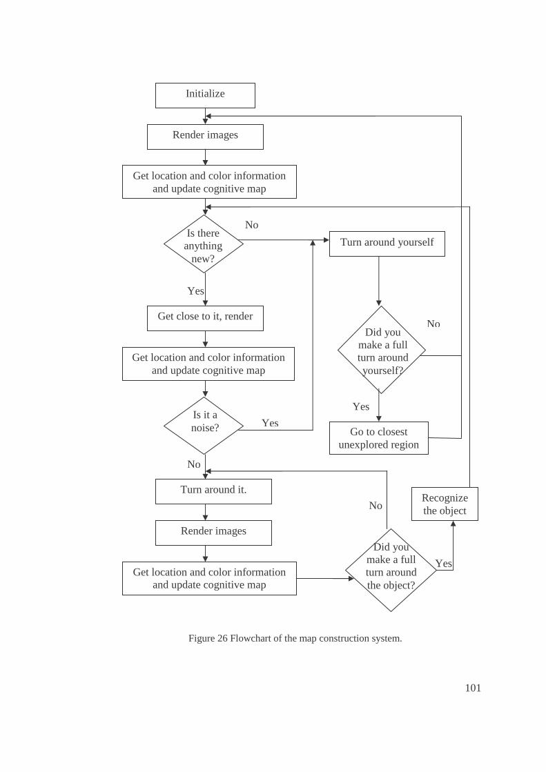
101
Figure 26 Flowchart of the map construction system.
Initialize
Render images
Get location and color information and update cognitive map
Is there anything
new?
Get close to it, render
Is it a noise?
Turn around it.
Render images
Get location and color information and update cognitive map
Calculate location and color
Did you make a full turn around the object?
No
No
Yes
Yes
Turn around yourself
Did you make a full turn around yourself?
No
No
Go to closest unexplored region
Yes
Recognize the object
Get location and color information and update cognitive map
Yes

102
Figure 27 3D cognitive map. x- and z- axis are the width and depth of the environment
respectively and y-axis is for height above the ground. Only the grids for which the belief of being occupied are high are shown here. Others are given zero values i.e. not occupied.
4.5 Object Recognition
While exploring the environment for the purpose of map construction, whenever a
new object is seen, the agent gets close to that object and turns around it keeping a
clearance between the object and itself and gets the 3D feature point locations of
that object. These locations are (x,y,z) triples..
While filling the cognitive map, the RGB color information is also saved for
each grid. This is done by following a few steps: First the averages of the RGB
values for each feature point are calculated. This is done by averaging the RGB
values of the pixels falling into a window centered at a feature point selected on the
right image of the stereo pair. Then the averages of the RGB values of the feature
points falling on the same grid are calculated. Finally the RGB averages for each
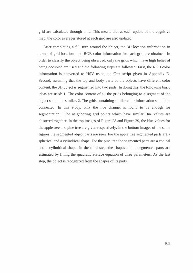
103
grid are calculated through time. This means that at each update of the cognitive
map, the color averages stored at each grid are also updated.
After completing a full turn around the object, the 3D location information in
terms of grid locations and RGB color information for each grid are obtained. In
order to classify the object being observed, only the grids which have high belief of
being occupied are used and the following steps are followed: First, the RGB color
information is converted to HSV using the C++ script given in Appendix D.
Second, assuming that the top and body parts of the objects have different color
content, the 3D object is segmented into two parts. In doing this, the following basic
ideas are used: 1. The color content of all the grids belonging to a segment of the
object should be similar. 2. The grids containing similar color information should be
connected. In this study, only the hue channel is found to be enough for
segmentation. The neighboring grid points which have similar Hue values are
clustered together. In the top images of Figure 28 and Figure 29, the Hue values for
the apple tree and pine tree are given respectively. In the bottom images of the same
figures the segmented object parts are seen. For the apple tree segmented parts are a
spherical and a cylindrical shape. For the pine tree the segmented parts are a conical
and a cylindrical shape. In the third step, the shapes of the segmented parts are
estimated by fitting the quadratic surface equation of three parameters. As the last
step, the object is recognized from the shapes of its parts.
104
(a)
(b) (c)
Figure 28 a. Location and color information stored in each grid for an apple tree in the
cognitive map, b. Cognitive map grids for the top of the apple tree, c. Cognitive map grids for the body of the apple tree.
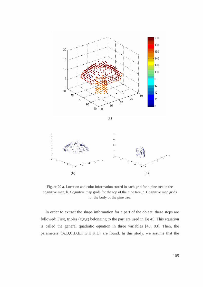
105
(a)
(b) (c)
Figure 29 a. Location and color information stored in each grid for a pine tree in the
cognitive map, b. Cognitive map grids for the top of the pine tree, c. Cognitive map grids
for the body of the pine tree.
In order to extract the shape information for a part of the object, these steps are
followed: First, triples (x,y,z) belonging to the part are used in Eq 45. This equation
is called the general quadratic equation in three variables [43, 83]. Then, the
parameters { A,B,C,D,E,F,G,H,K,L} are found. In this study, we assume that the

106
parameter A in Eq 45 is non-zero, since the shapes in our environment is either
sphere, cylinder or cone. Reorganizing Eq 45 we obtained Eq 46 and the unknown
equation parameters P={ B’ ,C’ ,D’ ,E’ ,F’ ,G’ ,H’ ,K’ ,L’ } can be solved as in Eq 47
where V�
is the pseudo inverse of V (Eq 48) and X is the vector of x-coordinates
(Eq 49). Here N is the total number of (x,y,z) triples. Finally, form these parameters
we can comment on the shape [43, 83].
0222222222 =+++++++++ LKzHyGxFyzExzDxyCzByAx Eq 46
222 222222 xLzKyHxGyzFxzExyDzCyB −=′+′+′+′+′+′+′+′+′ Eq 47
XV
L
K
H
G
F
E
D
C
B
P *�
=
������������
�
�
������������
�
�
′′′′′′′′′
= Eq 48
V=
���������
�
�
���������
�
�
1222222...............................................................1222222
.
22
11111111121
21
NNNNNNNNNNN zyxzyzxyxzy
zyxzyzxyxzy
Eq 49

107
X=
���������
�
�
���������
�
�
2
21
.
.
.
.
.
.
.
Nx
x
Eq 50
In order to comment on the shape, first of all an S matrix (Eq 50) and Q vector
(Eq 51) are formed from the parameters. This S matrix is a non-zero real symmetric
matrix [43, 83] and has real characteristic values, i.e. real eigenvalues � 1, � 2, � 3 ,
where at least one of them is different than zero. Since we deal with 3 basic shapes
of sphere, cone and cylinder, we can say that all three are different than zero. Thus,
there exists an orthogonal matrix R such that Eq 52 holds. Considering the change
of coordinates xx TR= where ),,( zyx=x , Eq 45 can be rewritten as Eq 53 where
',',' KHG are calculated as in Eq 54. Here, u1, u2, u3 are the eigenvectors of S.
Knowing that all three of the eigenvalues are non-zero, we can translate x system to
x~ system by 1
'~λG
xx += , 2
'~λH
yy += , 3
'~λK
zz += . Then Eq 53 can be rewritten as
in Eq 55 where k is calculated as in Eq 56.
���
�
�
���
�
�
′′′′′′′′
=CFE
FBD
ED
S
1
Eq 51
���
�
�
���
�
�
′′′
=K
H
G
Q Eq 52
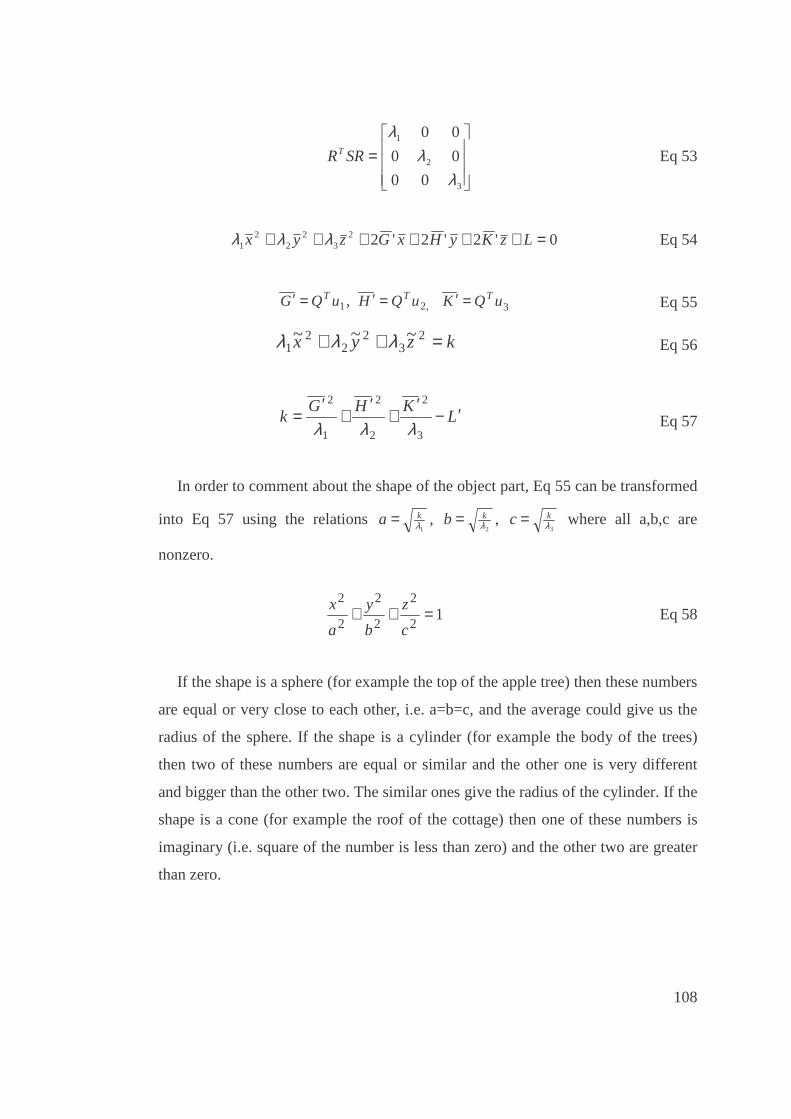
108
���
�
�
���
�
�
=
3
2
1
00
00
00
λλ
λSRRT Eq 53
0'2'2'223
22
21 =++++++ LzKyHxGzyx λλλ Eq 54
3,21, uQKuQHuQG TTT =′=′=′ Eq 55
kzyx =++ 23
22
21
~~~ λλλ Eq 56
LKHG
k ′−′
+′
+′
=3
2
2
2
1
2
λλλ Eq 57
In order to comment about the shape of the object part, Eq 55 can be transformed
into Eq 57 using the relations 1λ
ka = , 2λ
kb = , 3λ
kc = where all a,b,c are
nonzero.
12
2
2
2
2
2=++
c
z
b
y
a
x Eq 58
If the shape is a sphere (for example the top of the apple tree) then these numbers
are equal or very close to each other, i.e. a=b=c, and the average could give us the
radius of the sphere. If the shape is a cylinder (for example the body of the trees)
then two of these numbers are equal or similar and the other one is very different
and bigger than the other two. The similar ones give the radius of the cylinder. If the
shape is a cone (for example the roof of the cottage) then one of these numbers is
imaginary (i.e. square of the number is less than zero) and the other two are greater
than zero.

109
After finding the shape for both of the object parts, the object is recognized using
the following logic:
* If there is a sphere on a small radius cylinder, this is an apple tree.
* If there is a cone on a small radius cylinder, this is a pine tree.
* If there a cone is on a big cylinder, this is a cottage.
After going around the environment and recognizing all the objects seen, we
finally have the location information for all the objects and label for each of them.
In Figure 30 the 2D occupancy map and estimated labels for the objects are shown.
2D map is calculated by summing the grid values of 3D map in y-axis which gives
us the usual 2D environmental map.
Figure 30 Labeled occupancy.

110
4.6 Results and Conclusion
Some other virtual environments and the resultant 3D map and 2D occupancy
information are given in the following figures. In Figure 31 the environment is
constructed such that there is one from each object class and each of them is placed
very far away from the others. In Figure 32 the environment consists of three apple
trees which have different sizes. In all cases, map construction and object
recognition are successfully completed.
(a)
Figure 31 a. Virtual environment with three different object very far away from each other,
b. Computed 3D map, c. Occupancy (top view of 3D map) with labeled objects.
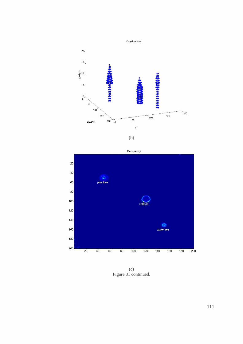
111
(b)
(c) Figure 31 continued.
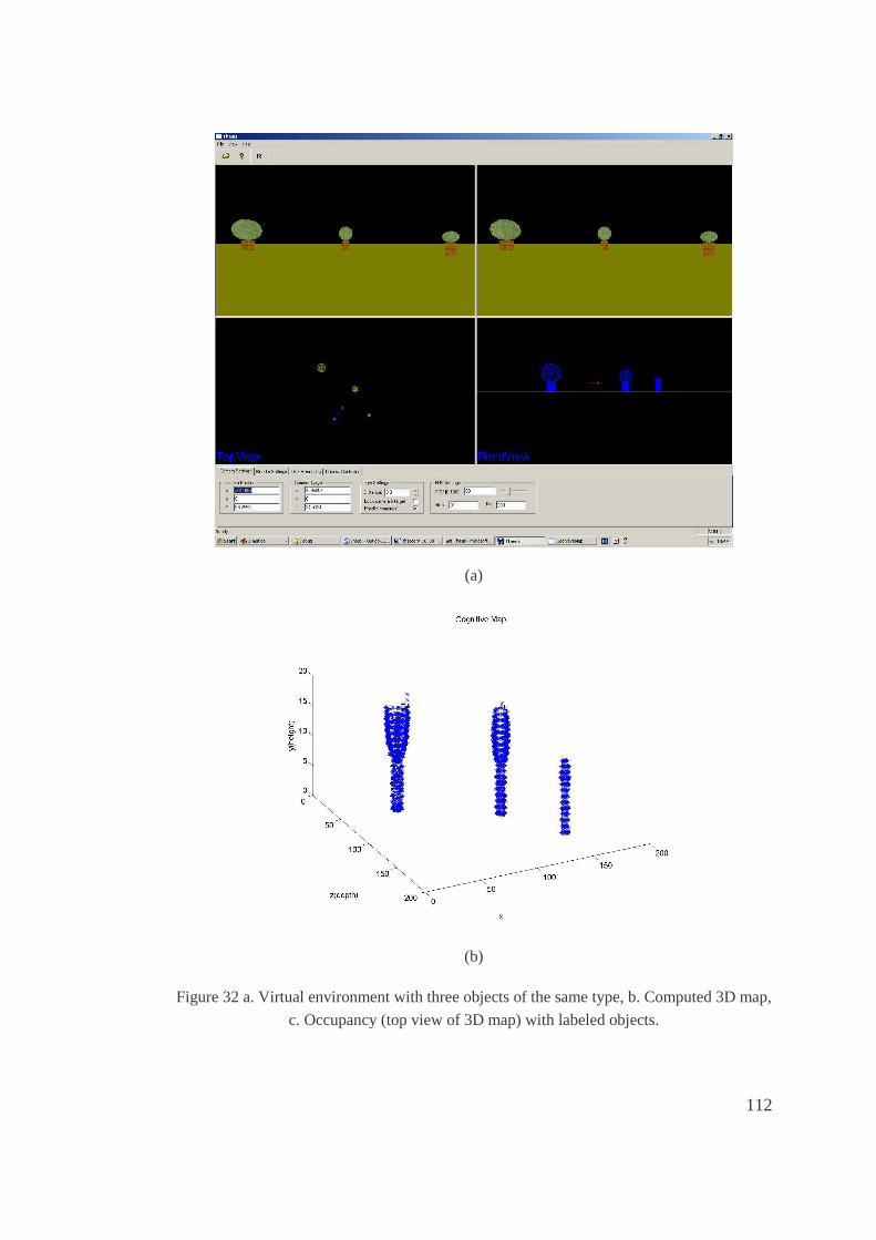
112
(a)
(b)
Figure 32 a. Virtual environment with three objects of the same type, b. Computed 3D map,
c. Occupancy (top view of 3D map) with labeled objects.

113
(c)
Figure 32 continued
The parameters used in our program are listed in the following table. Parameter
names, purposes and default values are listed in the successive columns from left to
right. These parameters are kept the same in all cases of map construction. A global
world coordinate system is assumed and the virtual world is centered at the center
of the world coordinate system. Virtual world is divided into grids of size GridSize
in world units in each dimension. The size of the stereo images rendered from the
virtual world is ImWidth by ImHeight pixels and kept the same through out the
process of map construction. Distance between stereo camera pairs (BaseLine in
world units), focal length of the cameras (FocalLength in world units), field of view
(FOV degrees), the nearest distance cameras can see (Near in world units) and the

114
farthest distance (Far in world units) are the camera parameters initialized at the
beginning of each map construction. MaxDisparity, MinDisparity and
RowPermission all in pixels are the limits of search space for disparity.
While the agent explores the environment, it keeps a distance of ObjectClearance
in world unit between the closest object in the view and itself. Also the same
distance is kept while turning around an object. The agent turns around the object
with ObjectTurnAngle degrees at each step of turn, and turns around itself with
RobotTurnAngle degrees at each step of turn.
After completing a full turn around an object, the point cloud belonging to the
object is thresholded by CountThreshold and the grids which have higher values are
selected and considered for the recognition step. Object is segmented into two
partsin terms of proximity and color similarity, where hue channel similarity is
enough in most cases and the ColorThreshold_Hue is the similarity threshold used.

115
Table 4 Parameters used in the program.
Name of the parameter Purpose Default value
ImWidth Image width 256 ImHeight Image height 256 WorldX Size of the virtual world in x
direction 200
WorldY Size of the virtual world in y direction
200
WorldZ Size of the virtual world in z direction
30
GridSize
Size of a single world grid in terms of world meters
1
BaseLine Distance between stereo cameras 0.3 FocalLength Focal length of the cameras 0.1 FOV Field of View 80º Far The farthest distance seen by the
cameras 100
Near The nearest distance seen by the cameras
0.1
MaxDisparity Maximum disparity search limit in epipolar direction
20
MinDisparity Minimum disparity search limit in epipolar direction
-10
RowPermission Search limit in the direction vertical to epipolar direction
1
CountThreshold The grid value threshold in order to be considered as occupied
5
ColorThreshold_Hue Hue similarity threshold 7.0 ColorThreshold_saturation Saturation similarity threshold 0.15 ColorThreshold_value Value similarity threshold 0.15 ObjectTurnAngle Amount of turn around the object at
each step 40º
RobotTurnAngle Amount of turn around the robot itself at each step
45º
ObjectClearance Distance kept between the robot and the object
10

116
CHAPTER 5
CONCLUSION
In this study a human-like disparity estimation algorithm for the purpose of depth
extraction is developed. Then this stereo vision system is applied to construct a
world centric, grid based cognitive map which is very important for higher
vertebrate survey navigation. This is done in a 3D virtual environment by moving a
virtual robot around the 3D objects of this virtual world. The future study is to apply
the algorithm on a real robot in a natural environment.
Navigation could not be achieved unless distance information is obtained. The
most informative, natural and cheapest sensors for depth extraction are stereo or
multiple cameras. With some processing on the images obtained by cameras, not
only distance but other information such as color, texture, shape, motion, etc. can be
obtained as well. And this brings the effort to include cameras as sensors to recent
robotic applications although extraction of information from multiple images is very
hard. By this way, a robot can simultaneously navigate, avoid obstacles, recognize
objects around, perform some very special tasks just like humans do when at least a
stereo camera pair is used as sensors. The final goal of many studies is to come up
with a system which functions as humans do. Thus a vision model which is similar
to human vision system would be very appropriate in order to perform many tasks
simultaneously in a parallel manner.
In this study, a disparity algorithm which is based on multi-scale phase similarity
of edges between corresponding feature points is developed. Sparse algorithms are

117
very important because before a dense analysis, at least in order to calibrate
cameras, sparse feature matching is needed. Also, for 3D reconstruction and many
robotic applications feature based methods work very well. In this study, features
and their orientation information are extracted from stereo image pairs by steerable
filters inspired from biological model of human cortical hyper-column structure
where responses to filters at various orientations are stored. Thus, instead of
calculating disparities using oriented filters and pooling the results over different
orientations, a single orientation for each feature is obtained prior to disparity
computation. The steerable filter estimate of stimulus orientation found using this
method is very accurate given the small number of filters used.
Although the feature points are sparse, since features are extracted using a multi-
scale strategy and they are the points of high contrast edges that define the bounding
contours of objects, they prove to be highly informative. Correspondences between
feature points are located using multi-scale phase information. This idea is
biologically grounded. The reason for this is that simple binocular cells occur in
pairs that are in quadrature phase. Besides, phase is very sensitive to position
differences hence it provides fine image detail which is helpful in discriminating
neighboring image regions and also is stable to geometric, lighting and very small
scale deformations. However phase may not be stable for large scale deformations.
There are image locations where phase is singular and can not be reliably used.
Such points are the locations where local frequencies are very different from the
filter tuning. Using multi-scale and including magnitude in matching algorithms
bring good results in matching images with scale deformations. In this study, phase
comparison is done at multiple scales and confidence weighting is used to augment
phase information with information concerning the magnitude of the steerable
filtered image to improve the correspondence method. Since phase-based stereo
methods are not good in textureless regions but only good at boundaries, using
multi-scale phase information at sparse feature points and using magnitude as
confidence provide a highly trustable disparity information at feature points only.

118
Two routes to locating feature-point correspondences are explored. Using the
position shift model, rough disparity values are obtained and a large range of
disparities can be calculated, but to a limited accuracy. Using the phase shift model,
fine tuning is performed without encountering the quarter cycle limit. This tuning
scheme also allows a continuum of disparity estimates to be obtained.
In the future studies, post processing will be performed on the disparity values in
order to get rid of spikes and discontinuities. Also, surface fitting will be applied to
sparse disparity results in order to obtain dense disparity. This will provide a tool
for image segmentation when color and disparity are used together.
Also, a probabilistic algorithm for correspondence matching is proposed.
Mixture of von Mises distributions are used to model probabilistic matching
algorithm using phase differences obtained for a stereo image pair and the model is
verified on other stereo pairs. Thus, it can be concluded that multi-scale phase
similarity is a good measure for sparse feature matching problems. In the future
studies, more number of stereo pairs will be used as training set in modeling our
algorithm probabilistically which will increase the success rate.
Finally, our stereo vision algorithm is applied in a simulated world. In this world
there is a virtual robot (agent) which has a stereo imaging system modeled with the
properties of human eye. There are also 3D objects which are made of simple
shapes such as sphere, cone, cylinder, etc. In our study, the agent explores its
environment based on some heuristics and simultaneously builds a 3D map and
recognizes the objects it observes during exploration. The task of generating robot
motion in the pursuit of building a map is commonly referred to as robotic
exploration. While optimal robot motion is relatively well-understood in fully
modeled environments, exploring robots have to cope with partial and incomplete
models. Hence, any viable exploration strategy has to be able to accommodate
contingencies and surprises that might arise during map acquisition. For this reason,
exploration is a challenging planning problem, which is often solved sub-optimally
via simple heuristics. In future studies, more complex objects will be used in our

119
virtual world and our virtual world will include natural effects such as lighting,
background, shadow ect.
In the future studies, our exploration strategy will be expanded and our complete
system will be applied on real robots. In that case simultaneous localization and
mapping, ego-motion extraction problems will also be studied. All these problems
are very closely related to stereo matching and with some slight changes on our
algorithm we would be able to provide results for these problems also. Our final
goal is to have a system where obstacle avoidance, map construction, localization,
ego-motion extraction, object recognition and 3D reconstruction are done
simultaneously. Also auto focusing which is very important for calibration and
deciding on search space will be investigated.
In our study we only used world-centric coordinate system. However, human can
prefer ego-centric or world-centric coordinate system with respect to the task
performed. Thus, using ego-centric and world-centric together according to task is
an other future study.
120
REFERENCES
[1] Anzai, A., Ohzawa, I., Freeman, R. D., Neural mechanisms for encoding binocular disparity: Receptive field position vs. phase. Journal of Neurophysiology, vol. 82, no. 2, pp. 874-890, 1999.
[2] Anzai, A., Ohzawa, I., Freeman, R. D., Neural mechanisms for processing binocular
information: I. Simple cells. Journal of Neurophysiology, vol. 82, no. 2, pp. 891-908, 1999.
[3] Anzai, A., Ohzawa, I., Freeman, R. D., Neural mechanisms for processing binocular
information: II. Complex cells. Journal of Neurophysiology, vol. 82, no. 2, pp. 909-924, 1999.
[4] Baker, S., Szeliski, R., Anandan, P., A layered approach to stereo reconstruction,
Proc. of CVPR98, pp. 434-441, 1998. [5] Baluja, S., Pomerleau, D. A., Expectation based selective attention for visual
monitoring and control of a robot vehicle. Robotics and Autonomous Systems 22, pp. 329-344, 1997.
[6] Bishop, C. M., Neural Networks for Pattern Recognition. Oxford University Press,
1995. [7] Blake, R., Wilson, H.R., Neural models of stereoscopic vision. Trends in
Neuroscience, vol. 14, no. 10, pp.445-452, 1991. [8] Carneiro, G., Jepson, A.D., Phase-based local features. In ECCV2002, pp. 282-296,
Copenhagen, Denmark, May 2002. [9] Carneiro, G., Jepson, A.D., Multi-scale phase-based local features. In CVPR, pp.
736-743, Madison, WI, USA, June 2003. [10] Cartwright, B. A., Collett, T. S., Landmark learning in bees. Journal of
Computational Physiology A 151, pp.521-543, 1983. [11] Coombs, D., Roberts, K., Centering behavior using peripheral vision. Proceedings of
IEEE Conference on Computer Vision and Pattern Recognition, IEEE Computer Society Press, Los Alamitos, CA, pp. 440-451, 1993.

121
[12] Cox, I., Hingorani, S., Rao, S., A maximum likelihood stereo algorithm. Computer Vision and Image Understanding, vol. 63, no. 3, May 1996.
[13] Daugman, J., Uncertainity relation for resolution in space, spatial frequency and
orientation optimized by two dimensional visual cortical filters. Journal of the Optical Society of America 2, pp. 1160-1169, 1985.
[14] Davison, A. J., Murray, D. W., Simultaneous localization and map building using
active vision, IEEE transactions on Pattern Analysis and Machine Intelligence, vol. 24, no. 7, pp. 865-880, July 2002.
[15] DeAngelis, G., Seeing in three dimensions: the neurophysiology of stereopsis. Trends
in Cognitive Science, vol. 4, no. 3, s. 80-89, 2000. [16] DeSouza, G. N., Kak, A.C., Vision for mobile robot navigation: A Survey. IEEE
Transactions on Pattern Analysis and Machine Intelligence, vol. 24, no. 2, pp. 237-267, 2002.
[17] Elder, J. H., Zucker, S. W., Locale scale control for edge detection and blur
estimation. IEEE PAMI, 20 (7), pp. 699-716, 1998. [18] Erol, A., Automatic Fingerprint Recognition. Ph.D. Thesis, Middle East Technical
University, Electrical and Electronics Department, Ankara, Turkey, 2001. [19] Erwin, E., Miller, K. D. The subregion correspondence model of binocular simple
cells. Journal of Neuroscience 19, pp. 7212-7229, 1999. [20] Fischler, M. A., Bolles, R. C., Random sample consensus: a paradigm for model
fitting with application to image analysis and automated cartography. Communication Association and Computing Machine, 24 (6), pp. 381-395, 1981.
[21] Fleet, D., Measurement of Image Velocity. Kluwe Academic Publishers, 1992. [22] Fleet, D. J., Wagner, H.,Heeger, D. J., Neural encoding of binocular disparity:
Energy models, position shifts and phase shifts. Vision Research, vol. 36, no. 12, pp. 1839-1857, 1996.
[23] Franz, M.O., Schölkopf, B., Mallot, H. A., Bülthoff, H. H., Leaning view graphs for
robot navigation. Autonomous Robots, 5, pp. 111-125, 1998. [24] Franz, M. O., Mallot, H. A., Biomimetic robot navigation. Robotic and Autonomous
Systems, 30, pp. 133-153, 2000. [25] Freeman, R. D., Ohzawa, I., On the neurophysiological organization of binocular
vision. Vision Research, vol. 30, no. 11, pp. 1661-1676, 1990. [26] Freeman, W. T., The design and use of Steerable Filters. IEEE Trans. Pattern
Analysis and Machine Intelligence, 13(9), 1991.

122
[27] Fröhlinghaus, T., Buhmann, J. M., Regularizing phase-based stereo. International
Conference on Pattern Recognition, ICPR96, pp. 451-455, Vienna, 1996. [28] Fua, P., Leclerc, Y. G., Using 3D meshes to combine image-based and geometry-
based constraints. In ECCV94, pp. B:281-291, 1994. [29] Fua, P., From multiple stereo views to multiple 3-D surfaces. International Journal of
Computer Vision, 24 (1):19-35, 1997. [30] Gaussier, P., Joulain, C., Zrehen, S., Revel, A., Visual navigation in an open
environment without map. Proc. IEEE Int’ l Conf. Intelligent Robots and Systems, pp. 545-550, Sept. 1997.
[31] Gaussier, P., Lepretre, S., Joulain, C., Revel, A., Quoy, M., Banquet, J. P., Animal
and robot learning: experiments and models about visual navigation. In Seventh European Workshop on Learning Robots- EWLR'98, Edinburgh, UK, 1998.
[32] Georgopoulos, A. P., Schwarz, A. B., Kettner, R. E., Neural population coding of
movement direction. Science 233, pp. 1416-1419, 1986. [33] Grimson, W. A computer implementation of a theory of human stereo vision. Royal,
B-292:217-253, 1981. [34] Harris, C., Determination of ego-motion from matched points. Proc. Alvey Vision
Conf., 1987. [35] Harris, C., Stephens, M., A combined corner and edge detector. In Alvey Vision
Conference, pp. 147-151, 1988. [36] Hüber, S. A., Bülthoff, H. H., Simulation and robot implementation of visual
orientation behaviors of flies. In: Pheifer, R., Blumberg, B., Meyer, J. A., Wilson, S. W. (Eds.), From Animals to Animats 5, Proceedings of SAB’98, MIT Press, Cambridge, MA, pp.77-85, 1998.
[37] Jenkin, M. R. M., Jepson, A. D., Recovering local surface structure through local
phase difference measurements. CVGIP: Image Understanding, vol. 59, no. 1, pp. 72-93, 1994.
[38] Jepson, A. D., Fleet, D. J., Scale space singularities. Lecture Notes in Computer
Science, vol. 427, pp. 50-55, 1990. [39] Jepson, A. D., Fleet, D. J., Phase singularities in scale space. Image and Vision
Computing, vol. 9, no. 5, s. 338-343, 1991. [40] Jones, D. G., Malik, J., Computational framework for determining stereo
correspondence from a set of linear spatial filters. Image and Vision Computing, vol. 10, no. 10, pp. 699-708, 1992.

123
[41] Jerbic, B., Grolinger, K., Vranjes, B., Autonomous agent based on reinforcement
learning and adaptive shadowed network. Artificial Intelligence in Engineering 13, pp. 141-157, 1999.
[42] Kagami, S., Okada, K., Inaba, M., Inoue, H., Design and implementation of on body
real-time depth map generation system. Proceedings of the 2000 IEEE International Conference on Robotics and Automation, San Francisco, CA, pp. 1441-1446, April 2000.
[43] Karaka� , H. I. Analytic Geometry. [44] Kim, D., Nevatia, R., Symbolic navigation with a generic map. Proc. IEEE Workshop
Vision for Robots, pp. 136-145, Aug. 1995. [45] Kundur, S. R., Raviv, D., Active vision based control schemes for autonomous
navigation tasks. Pattern Recognition 33, pp. 295-308, 2000. [46] Lee, S. H., Park, J. I., Lee, C. W., A new stereo matching algorithm based on
Bayesian model. Proc. IEEE ICASSP98, pp. 2769-2772, 1998. [47] Lelo� lu, U. M., Halıcı, U., Multi-image region growing for integrating disparity
maps. In Franc Solina and Ales Leonardis, editors, Computer Analysis of Images and Patterns, CAIP99, pp. 403-410, Slovenia, 1999.
[48] Leven, P., Hutchinson, S., Burschka, D., Farber, G., Perception based motion
planning for indoor exploration, Prooceedings of the 1999 IEEE International Conference on Robotics and Automation, Detroit, Michigan, pp. 695-701, May 1999.
[49] Li, G., Svensson, B., Navigation with a focus directed mapping network.
Autonomous Robots 7, pp. 9-30, 1999. [50] Lowe, D.G., Three-dimensional object recognition in it cortex. In First IEEE
International Workshop on Biologically Motivated Computer Vision, pg. 20-31, Seoul, Korea, May 2000.
[51] Ludtke, N., Wilson, R. C., Hancock, E. R., Tangent fields from population coding.
Lecture Notes in Computer Science, vol. 1811, pp. 584-593, 2000. [52] Marr, D., Poggio, T., A computational theory of human stereo vision. Proceedings of
the Royal Society of London, B207, pp. 187-217, 1979. [53] Marshall, J. A., Burbeck, C. A., Ariely, D., Occlusion edge blur: a cue to relative
visual depth. Journal of the Optical Society of America, 1996. [54] Mataric, M. J., Navigation with a rat brain: A neurobiologically inspired model for
robot spatial representation. In: Meyer, J. A., Wilson, S. W. (Eds.), Form Animals to Animats, MIT Press, Cambridge, MA, 1991.

124
[55] Matsumoto, Y., Inaba, M., Inoue, H., Visual navigation using view-sequenced route
representation. Proc. IEEE Int’ l Conf. Robotics and Automation, vol. 1, pp. 83-88, Apr. 1996.
[56] Mayhew, J. E. W., Frisby, J. P. , Psychophysical and computational studies towards a
theory of human stereopsis. Artificial Intelligence, vol. 17, pp. 349-385, 1981. [57] Medioni, G., Nevatia, R. Segment-based stereo matching. CVGIP, 31(1), pp.2-18,
1985. [58] Meng, M., Kak, A. C., Mobile robot navigation using neural networks and
nonmetrical environment models. IEEE Control Systems, pp. 30-39, Oct. 1993. [59] Moallem, P., Faez, K., Haddadnia, J., Reduction of the search space region in the
edge based stereo correspondence. VMV, pp. 149-152, 2001. [60] Moravec, H. P., Elfes, A., High resolution maps from angle sonar. In IEEE
International Conference on Robotics and Automation, pp. 116-121, 1985. [61] Murray, D., Little, J., Using real-time stereo vision for mobile robot navigation.
Prooceedings of the IEEE Workshop on Perception for Mobile Agents, Santa Barbara, CA, June 1998.
[62] Mülayim, A. Y., 3D Reconstruction of Rigid Objects from Multiple Calibrated
Views. Ph.D. Thesis, METU, Ankara, Turkey, 2003. [63] Myers, R., Wilson, R. C., Hancock, E.R., Bayesian graph edit distance. Image
Analysis and Processing, Venice, Italy, pp. 1166-1171, 1999. [64] Nelson, R.C., Memory based recognition for 3-d objects. In ARPA Image
Understanding Workshop, pg. 1305-1310, Palm Springs, USA, February 1996. [65] Nourbakhsh, I. R., Andre, D., Tomasi, C., Genesereth, M. R., Obstacle avoidance via
depth from focus, ARPA Image Understanding Workshop 1996. [66] Ohya, A., Kosaka, A., Kak, A., Vision based navigation by a mobile robot with
obstacle avoidance using single camera vision and ultrasonic sensing. IEEE Transactions on Robotics and Automation, vol. 14, no. 6, December 1998.
[67] Ohzawa, I., DeAngelis, G. C., Freeman, R. D., Stereoscopic depth discrimination in
the visual cortex: Neurons ideally suited as disparity detectors. Science, vol. 249, no. 4972, pp. 1037-1041, 1990.
[68] Ohzawa, I., Mechanisms of stereoscopic vision: the disparity energy model. Current
Opinion in Neurobiology 8, pp. 509-515, 1998.

125
[69] Okada, K., Kino, Y., Kanehino, F., Kuniyoshi, Y., Inaba, M., Inoue, H., Rapid development system for humanoid vision-based behaviours with real-virtual common interface. Proceedings of the International Conference on Intelligent Robotics and Systems, Laussanne, Switzerland, Oct 2002.
[70] Olson, C. F., Subpixel localization and uncertainty estimation using occupancy grids.
Proceedings of the 1999 IEEE International Conference on Robotics and Automation, Detroit, Michigan, pp. 1987-1992, May 1999.
[71] Olson, C. F., Maximum likelihood image matching. IEEE Transactions on Pattern
Analysis and Machine Intelligence, vol. 24, no 6, pp. 853-857, 2002. [72] Pentland, A. P., A new sense of depth of field. IEEE Trans. On Pattern Analysis and
Machine Intelligence, vol. PAMI-9, no 3, pp. 523-531, 1987. [73] Perez, J.A., Castellanos, J. A., Montiel, J. M. M., Neira, J., Tardos, J. D., Continuous
mobile robot localization: Vision vs. Laser, Proceedings of the 1999 IEEE International Conference on Robotics and Automation, Detroit, Michigan, pp. 2917-2923, May 1999.
[74] Pollard, S. B., Mayhew, J. E. W., Frisby, J. P., PMF: A stereo correspondence
algorithm using a disparity gradient limit. Perception, vol. 14, pp. 449-470, 1985. [75] Prescott, T. J., Spatial representation for navigation in animats. Adaptive Behaviour,
4(2), pp. 85-123, 1996. [76] Qian, N., Computing stereo disparity and motion with known binocular cell
properties. Neural Computation, vol. 6, no. 3, pp. 390-404, 1994. [77] Qian, N., Zhu, Y., Physiological computation of binocular disparity. Vision Research,
vol. 37, no. 13, s. 1811-1827, 1997. [78] Qian, N., Relationship between phase and energy methods for disparity computation.
Neural Computation, 12, pp. 279-292, 2000. [79] Quoy, M., Laroque, P., Gaussier, P., Learning and motivational couplings promote
smarter behaviors of an animate in an unknown world. Robotics and Autonomous Systems 38, pp. 149-156, 2002.
[80] Rabie, T. F., Terzopoulos, D., Stereo and color analysis for dynamic obstacle
avoidance. CVPR1998, pp. 245-252, 1998. [80] Ramloll, R., Mowat, D., Way finding in virtual environments using an interactive
spatial cognitive map. In IV2001 Proceedings, IEEE Press, pp. 574-583, 2001. [81] Recce, M., Harris, K. D., Memory of places: A navigational support of Marr’s theory
of hippocampal function. Hippocampus 6, pp. 735-748, 1996.
126
[82] Robert, L., Faugeras, O. Curve-based stereo: Figural continuity and curvature. In IEEE Conference on Computer Vision and Pattern Recognition, pp. 57-62, 1991.
[83] Rogers, D. F., Adams, J. A., Mathematical Elements for Computer Graphics. Second
Eddition, McGraw-Hill International Editions, 1990. [84] Sanger, T. D., Stereo disparity computation using Gabor filters. Biol. Cybern., 59, pp.
405-418, 1988. [85] Scharstein, D., Szeliski, R., A Taxonomy and evaluation of dense two-frame stereo
correspondence algorithms. International Journal of Computer Vision, 47 (1/2/3), pp. 7-42, April-June 2002.
[86] Schmid, C., Mohr, R., Local gray value invariants for image retrieval. IEEE
Transactions on Pattern Analysis and Machine Intelligence, 19(5):530-535, 1997. [87] Schmitt, M., Rous, M., Matsikis, A., Kraiss, K. F., Vision-based self-localization of a
mobile robot using a virtual environment. Proceedings of the International Conference on Robotics and Automation, Detroit, Michigan, pp. 2911-2916, May 1999.
[88] Schölkopf, B., Mallot, H., View-based cognitive mapping and path planning.
Adaptive Bahavior, 3, pp. 311-348, 1995. [89] Se, S., Lowe, D., Little, J., Vision-based mobile robot localization and mapping using
scale-invariant features. Proceedings of the 2001 IEEE International Conference on Robotica and Automation, Seoul, Korea, pp.2051-2058, May 2001.
[90] Terzopoulos, D., Rabie, T. F., Animat vision: Active vision in artificial animals.
Journal of Computer Vision Research, pp. 2-19, September, 1997. [91] Thrun, S., Learning metric-topological maps for indoor mobile robot navigation.
Artificial Intelligence, 99 (1), pp. 21-71, 1998. [92] Thrun, S., Learning occupancy grids with forward models. Proceedings of the 2001
IEEE/RSJ International Conference on Intelligent Robots and Systems, Mani, Hawaii, USA, pp.1676-1681, Oct.29-Nov. 03, 2001.
[93] Torr, P.H.S., Zisserman, A., Feature-based methods for structure and motion
estimation. In Vision Algorithms: Theory and Practice, pg. 278-294, Corfu, Greece, September 1999.
[94] Tunçer, F., Image Synthesis for Depth Estimation Using Stereo and Focus Analysis.
M.Sc. Thesis, Department of Electrical and Electronics Engineering, Middle East Technical University, Ankara, Turkey, 2002.
127
[95] Vincent, E., Laganiere, R., Matching feature points in stereo pairs: A comparative study of some matching strategies. Int. Journal of Machine Graphics and Vision, vol. 10, no. 3, pp. 237-259, 2001.
[96] Vogels, R., Population coding of stimulus orientation by striate cortical cells.
Biological Cybernetics, 64, pp. 25-31, 1990. [97] Voicu, H., Schmayuk, N., Three dimensional cognitive mapping with a neural
network. Robotic and Autonomous Systems 35, pp. 23-36, 2001 . [98] Wolf, J., Burgard, W., Burkhardt, H., Robust vision-based localization for mobile
robots using an image retrieval system based on invariant features. Proceedings of the 2002 IEEE International Conference on Robotics and Automation, Washington, DC, pp. 359-365, May 2002.
[99] Zucker, S., Early orientation selection: Tangent fields and the dimensionality of their
support, Comp. Vis., Graph., and Image Process., 32, pp. 74-103, 1985.

128
APPENDIX A
DEPTH PERCEPTION IN HUMAN VISUAL SYSTEM
The visual system makes use of a variety of cues to help judge the distance of
objects. These cues can be classified mainly into two groups:
• Monocular (pictorial) cues
• Binocular cues
A.1 Pictor ial Depth Cues
Our perception of the relative depth, or distance from the viewpoint, of the various
objects in a static, two-dimensional image of a three-dimensional scene may be
influenced to various extents by several different factors, which are sometimes
referred to as pictorial cues to depth because of their use by artists to convey a
greater sense of depth in a flat medium.
A.1.1 Occlusion (Interposition)
Probably the most important of the pictorial depth cues is occlusion, the obscuration
of a portion of a more distant object’s surface by another surface that is closer to the
viewpoint. There is evidence that our visual system makes fundamental use of
occlusion information to encode the relative depths of superimposed surfaces at a
relatively early stage in visual processing, and that the occlusion boundaries are the

129
key elements in conveying the depth relationships. See Figure 33 for a illustration
of occlusion.
Figure 33 An illustration showing the effect of occlusion
A.1.2 L inear Perspective
When we look through our eyes at the world, the three-dimensional information in
the scene gets projected onto the two-dimensional surface of our retina.
Mathematically, this transformation can be described by a perspective projection, a
3D-to-2D mapping that has several important features. The first of these is what is
often referred to in the literature as “ linear perspective” or the observation that lines
which are parallel in the three-dimensional model will appear in the projected image
to converge toward a single vanishing point as they recede into the distance. This
phenomenon is illustrated in Figure 34. In general, the effect will be most
pronounced when the lines originate close to the viewpoint and extend a
considerable distance away.

130
Figure 34 An illustration showing linear perspective
Parallel lines are obviously not the only lines whose relative orientations are
“ remapped” by a perspective projection, but the effects of perspective convergence
may be most clearly represented by them. It becomes increasingly difficult to
appreciate the “distortion” due to perspective projection when the represented
objects are more distant from the viewpoint, have a more limited extent in depth,
and are smoothly curving or of irregular or unfamiliar shape.
A perspective projection is clearly not the only possible 3D-to-2D mapping, and in
some instances it has been argued that, for the purposes of representing certain
types of information about a three-dimensional model, it is not necessarily the best
type of mapping to use. A common alternative is to employ an orthographic
projection, in which parallel lines remain parallel. Such projections can be
somewhat easier to construct manually and interpret intellectually, and certain
algorithms for generating images from three-dimensional models derive their
computational efficiency from relying on the regularities inherent in this approach.

131
We are not constrained, when constructing a computer-generated image, to
represent the data exactly as it would appear if it sat before us as a physical entity;
however, it is important to consider both the advantages and disadvantages of
stylizing the display.
A.1.3 Relative familiar size
A second consequence of perspective (but not orthographic) projection is that as an
object moves farther away from the viewpoint it will subtend a smaller visual angle
on the retina. This means that more distant objects will have relatively smaller
projected sizes, and this is the basic premise behind the pictorial depth cue referred
to as “ relative familiar size” . Size is an ambiguous cue unless the physical size of
the object is known.
Figure 35 Relative size as a cue. Which one of the balloons looks closer?

132
A.1.4 Focus, Depth of Field and Accommodation
When we perceive objects in our everyday experience, we are rarely conscious of
anything appearing to be “out of focus” . Under ordinary circumstances, when we
direct our attention to an object we fixate it in our fovea and automatically adjust
the lens of our eye to bring the object into focus. Because of the great disparity
between the depth of field attainable by our visual system and the depth of field
available with a camera, however, it is not at all uncommon to observe photographs
in which some part of the image is blurred due to its distance in depth from the
focal point.
Accommodation refers to the ability of the eye to change focus from distant to
near objects.
Figure 36 Accommodation. Blurred image.
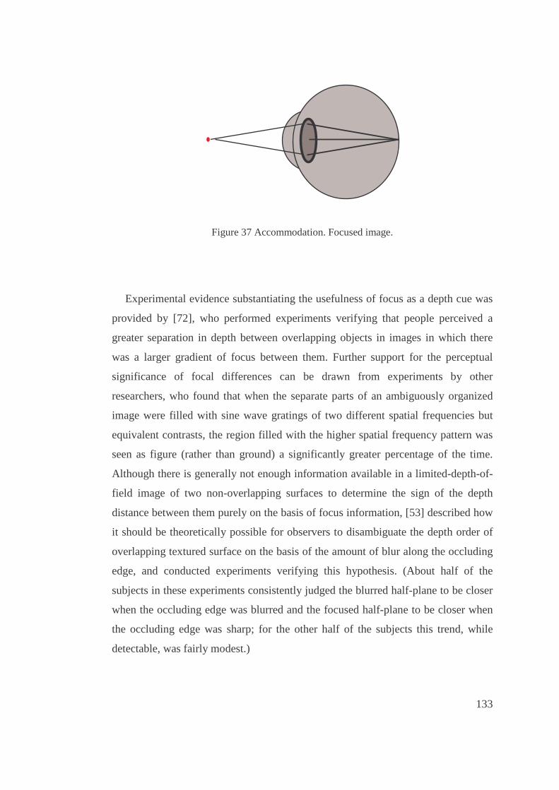
133
Figure 37 Accommodation. Focused image.
Experimental evidence substantiating the usefulness of focus as a depth cue was
provided by [72], who performed experiments verifying that people perceived a
greater separation in depth between overlapping objects in images in which there
was a larger gradient of focus between them. Further support for the perceptual
significance of focal differences can be drawn from experiments by other
researchers, who found that when the separate parts of an ambiguously organized
image were filled with sine wave gratings of two different spatial frequencies but
equivalent contrasts, the region filled with the higher spatial frequency pattern was
seen as figure (rather than ground) a significantly greater percentage of the time.
Although there is generally not enough information available in a limited-depth-of-
field image of two non-overlapping surfaces to determine the sign of the depth
distance between them purely on the basis of focus information, [53] described how
it should be theoretically possible for observers to disambiguate the depth order of
overlapping textured surface on the basis of the amount of blur along the occluding
edge, and conducted experiments verifying this hypothesis. (About half of the
subjects in these experiments consistently judged the blurred half-plane to be closer
when the occluding edge was blurred and the focused half-plane to be closer when
the occluding edge was sharp; for the other half of the subjects this trend, while
detectable, was fairly modest.)
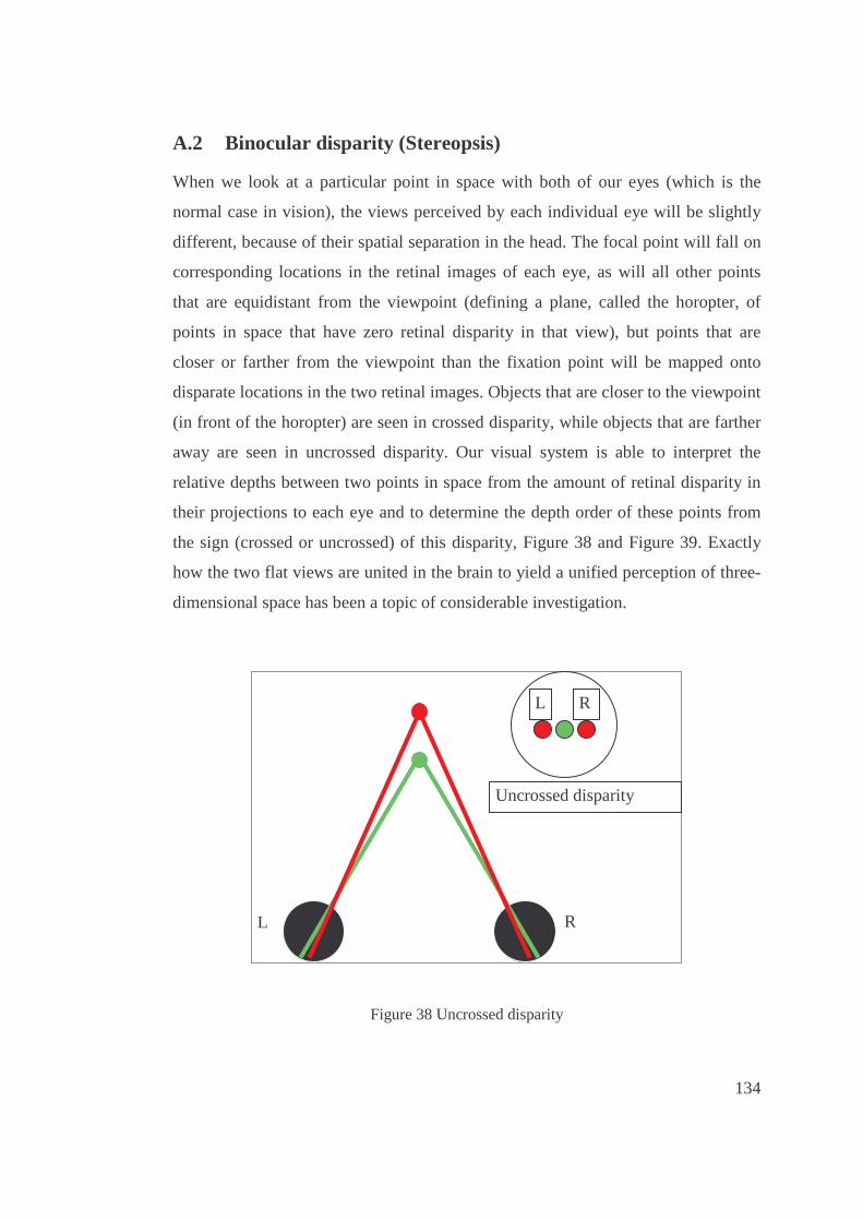
134
A.2 Binocular dispar ity (Stereopsis)
When we look at a particular point in space with both of our eyes (which is the
normal case in vision), the views perceived by each individual eye will be slightly
different, because of their spatial separation in the head. The focal point will fall on
corresponding locations in the retinal images of each eye, as will all other points
that are equidistant from the viewpoint (defining a plane, called the horopter, of
points in space that have zero retinal disparity in that view), but points that are
closer or farther from the viewpoint than the fixation point will be mapped onto
disparate locations in the two retinal images. Objects that are closer to the viewpoint
(in front of the horopter) are seen in crossed disparity, while objects that are farther
away are seen in uncrossed disparity. Our visual system is able to interpret the
relative depths between two points in space from the amount of retinal disparity in
their projections to each eye and to determine the depth order of these points from
the sign (crossed or uncrossed) of this disparity, Figure 38 and Figure 39. Exactly
how the two flat views are united in the brain to yield a unified perception of three-
dimensional space has been a topic of considerable investigation.
Figure 38 Uncrossed disparity
R L
Uncrossed disparity
R L
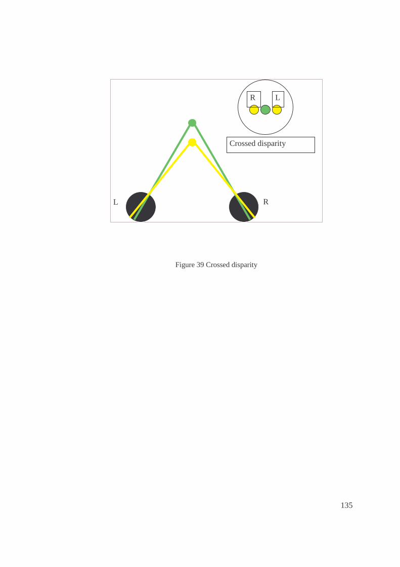
135
Figure 39 Crossed disparity
R L
Crossed disparity
R L

136
APPENDIX B
GEOMETRY FILE FORMAT
A sample geometry file listing with a few primitives is given below. The fields are
self-explanatory as seen from the comment lines.
# Shader count 3 # Texture count 9 # Visual count 13 ################################################################################ # SHADER 0 ################################################################################ # Ambient color 1.0 1.0 1.0 1.0 # Diffuse color 1.0 0.0 0.0 0.0 # Specular color 1.0 0.0 1.0 0.0 # Emissive color 0.0 0.0 0.0 0.0 # Shininess [0,128] 50 ################################################################################ # SHADER 1 ################################################################################

137
# Ambient color 0.0 0.0 1.0 1.0 # Diffuse color 0.0 0.0 1.0 0.0 # Specular color 1.0 1.0 1.0 1.0 # Emissive color 0.0 0.0 0.0 0.0 # Shininess [0,128] 50 ################################################################################ # SHADER 2 ################################################################################ # Ambient color 0.0 1.0 1.0 0.0 # Diffuse color 1.0 0.0 1.0 0.0 # Specular color 1.0 1.0 0.0 0.0 # Emissive color 0.0 0.0 0.0 0.0 # Shininess [0,128] 50 ################################################################################ # TEXTURE 0 ################################################################################ textures/checker.tga textures/wood.tga textures/brick.tga textures/grass.tga textures/roof.tga textures/sky.tga textures/earth.tga textures/cobra.tga textures/bubinga.tga ################################################################################ # VISUAL 0 - SPHERE TREE TOP - APPLE ################################################################################ # Visual type SPHERE # Center 10 12 20 # Radius 4

138
# Shader index -1 # Texture index 3 ################################################################################ # VISUAL 1 - TREE BODY - APPLE ################################################################################ # Visual type CYLINDER # RadiusBase 2 # RadiusTop 2 # Height 8 # Slices 50 # Stacks 30 # Translation [x,y,z] 10 8 20 # Rotation [x,y,z] 1 0 0 # Shader index -1 # Texture index 1 ################################################################################ # VISUAL 2 - HAUSE ################################################################################ # Visual type CYLINDER # RadiusBase 7

139
# RadiusTop 7 # Height 7 # Slices 70 # Stacks 80 # Translation [x,y,z] 20 7 -5 # Rotation [x,y,z] 1 0 0 # Shader index -1 # Texture index 2 ################################################################################ # VISUAL 3 - ROOF ################################################################################ # Visual type CYLINDER # RadiusBase 1 # RadiusTop 7 # Height 4 # Slices 36 # Stacks 50 # Translation [x,y,z] 20 11 -5 # Rotation [x,y,z] 1 0 0 # Shader index

140
-1 # Texture index 4 ################################################################################ # VISUAL 4 - SPHERE TREE TOP - APPLE ################################################################################ # Visual type SPHERE # Center -10 12 -30 # Radius 4 # Shader index -1 # Texture index 3 ################################################################################ # VISUAL 5 - TREE BODY - APPLE ################################################################################ # Visual type CYLINDER # RadiusBase 2 # RadiusTop 2 # Height 8 # Slices 50 # Stacks 30 # Translation [x,y,z] -10 8 -30 # Rotation [x,y,z]

141
1 0 0 # Shader index -1 # Texture index 1 ################################################################################ # VISUAL 6 - TREE TOP - PINE ################################################################################ # Visual type CYLINDER # RadiusBase 1 # RadiusTop 8 # Height 8 # Slices 36 # Stacks 20 # Translation [x,y,z] -10 16 -5 # Rotation [x,y,z] 1 0 0 # Shader index -1 # Texture index 3 ################################################################################ # VISUAL 7 - TREE BODY - PINE ################################################################################ # Visual type CYLINDER # RadiusBase 2

142
# RadiusTop 2 # Height 8 # Slices 36 # Stacks 20 # Translation [x,y,z] -10 8 -5 # Rotation [x,y,z] 1 0 0 # Shader index -1 # Texture index 1 ################################################################################ # VISUAL 8 - TREE TOP - PINE ################################################################################ # Visual type CYLINDER # RadiusBase 1 # RadiusTop 8 # Height 8 # Slices 36 # Stacks 20 # Translation [x,y,z] -40 16 -30 # Rotation [x,y,z] 1 0 0

143
# Shader index -1 # Texture index 3 ################################################################################ # VISUAL 9 - TREE BODY - PINE ################################################################################ # Visual type CYLINDER # RadiusBase 2 # RadiusTop 2 # Height 8 # Slices 36 # Stacks 20 # Translation [x,y,z] -40 8 -30 # Rotation [x,y,z] 1 0 0 # Shader index -1 # Texture index 1 ################################################################################ # VISUAL 10 - SPHERE TREE TOP - APPLE ################################################################################ # Visual type SPHERE # Center -40 12 5 # Radius 4

144
# Shader index -1 # Texture index 3 ################################################################################ # VISUAL 11 - TREE BODY - APPLE ################################################################################ # Visual type CYLINDER # RadiusBase 2 # RadiusTop 2 # Height 8 # Slices 50 # Stacks 30 # Translation [x,y,z] -40 8 5 # Rotation [x,y,z] 1 0 0 # Shader index -1 # Texture index 1 ################################################################################ # VISUAL 12 - GROUND ################################################################################ # Visual type POLYGON # Enable back face culling 1 # Shader index 1

145
# Texture index -1 # Vertex count 4 # Vertex data # x y z r g b a tu tv -500 0 -500 0.5 0.5 0.0 0.0 0 0 -500 0 500 0.5 0.5 0.0 0.0 3 0 500 0 500 0.5 0.5 0.0 0.0 3 3 500 0 -500 0.5 0.5 0.0 0.0 0 3

146
APPENDIX C
A SAMPLE CAMERACONTROLLER PLUGIN
CameraController .h
#ifndef __CAMERACONTROLLER_H #define __CAMERACONTROLLER_H #include "Simulation.h" class CCameraController { public: virtual ~CCameraController() { } virtual char *GetInfo() { return "Default Camera Controller"; } virtual char *GetResult() { return "Default result"; } virtual void Tick() = 0; virtual void SetSimulation( CSimulation *pSimulation ) = NULL; } ; #endif BasicCameraController .cpp #include "../CameraController.h" #define _PLUGIN_EXPORT __declspec( dllexport ) //////////////////////////////////////////////////////////////////////////////// class CBasicCameraController : public CCameraController { public:

147
CSimulation *m_pSimulation; float m_fTime; public: CBasicCameraController() { m_pSimulation = NULL; m_fTime = 0.0f; } virtual char *GetInfo() { return "Basic Camera Controller\x0d\x0aWritten by Fahri Tuncer"; } virtual char *GetResult() { return "No result"; } virtual void Tick(); virtual void SetSimulation( CSimulation *pSimulation ) { m_pSimulation = pSimulation; } } ; //////////////////////////////////////////////////////////////////////////////// // extern "C" __declspec (dllexport) void* __stdcall CreateInstance() extern "C" __declspec (dllexport) void *CreateInstance() { return new CBasicCameraController(); } //////////////////////////////////////////////////////////////////////////////// void CBasicCameraController::Tick() { float campos[3] = { 3.0f, 1.0f, 3.0f } ; campos[0] = 3.0f * cosf( m_fTime ); campos[1] = 2.0f * cosf( m_fTime ); campos[2] = 3.0f * sinf( m_fTime ); m_pSimulation->SetCameraPos( campos ); m_fTime += 0.1f; }

148
APPENDIX D
C++ SCRIPT FOR RGB TO HSV CONVERSION
// r,g,b values are from 0 to 1 // h = [0,360], s = [0,1], v = [0,1] //if s == 0, then h = -1 (undefined) void RGBtoHSV( float r, float g, float b, float *h, float *s, float *v ) { float min, max, delta; min = MIN( r, g, b ); max = MAX( r, g, b ); *v = max; // v delta = max - min; if( max != 0 ) *s = delta / max; // s else { // r = g = b = 0 // s = 0, v is undefined *s = 0; *h = -1; return; } if( r == max ) *h = ( g - b ) / delta; // between yellow & magenta else if( g == max ) *h = 2 + ( b - r ) / delta; // between cyan & yellow else *h = 4 + ( r - g ) / delta; // between magenta & cyan *h *= 60; // degrees if( *h < 0 ) *h += 360; }