Active Sound and Vibration Control: theory and applications Volume 25/3 || ANC Around a human's head

Chapter 10

Active noise control around #ahuman's head using an adaptiveprediction method

S. Honda and H. HamadaDepartment of Information and Communication Engineering, Tokio DenkiUniversity, Tokio, Japan, Email: [email protected]

This chapter introduces a new active noise control system for optimal controlof the sound field around a humanfs head. Geometrical arrangements of errormicrophones are proposed around the head in a diffused noise field. In orderto evaluate the controlled sound field, a rigid sphere theoretical model is usedas a human's head in the computer simulations.

In previous studies it was shown that the theoretical sphere model main-tains a good approximation of a head-related transfer function (HRTF) belowabout 5 kHz. In this chapter the relationship between the noise reduction andthe corresponding configuration of the error microphone and secondary sourcearrangement is evaluated. As a result, we found that the closely located sec-ondary sources to the sphere head give significant noise reduction in a largecontrol area. A possible arrangement of the error microphones is found to pro-vide an optimal result according to a given control strategy, such as flatness ofreduced sound pressure of the quiet zone.

10.1 Introduction

In this research the aim is to achieve an effective active noise control systemat both the listener's ears as well as at a relatively large area around his or

Downloaded 23 Aug 2012 to 128.59.62.83. Term of Use: http://digital-library.theiet.org/journals/doc/IEEDRL-home/info/subscriptions/terms.jsp

224 Active Sound and Vibration Control

her head, so that significant control can be expected even when the listenerslightly moves his or her head. For this purpose, we have recently introduceda new strategy for an ANC system, in which the sound field around a human'shead has been investigated under noise exposure visualisation techniques.

This was based on the perfect rigid sphere model which was applied asa theoretical model of a human's head. According to the previous work[211, 312, 313], this model maintained a good approximation of the head-related transfer function up to 5 kHz, so that we were now able to define thetheoretically calculated HRTF, referred to as the sphere head-related transferfunction (SHRTF), to examine acoustic properties around the head.

In an ANC system the effectiveness of noise reduction and its area stronglydepend on the primary and secondary sound field as well as on the performanceof the controller. If an adequate arrangement between the secondary sourceand the controlled point can be chosen, it is possible to manipulate the shapeof the equalised area. Increasing the number of secondary sources and controlpoints may allow the expansion of the quiet zone, although there is always arestriction on the number of them for practical appliactions [105, 191].

In this Chapter the discussion is focussed on producing a large quiet zoneusing only a small number of error microphones and secondary sources. Thenumber of secondary sources is chosen to be two for the typical case of theANC system to control two points at both the listener's ears. Fundamentalinvestigation is carried out for two different sound fields, these are: the freesound field in which the incoming direction of the primary source is known,and the diffused sound field. In addition, we also examine the ANC systemfor multiple control points to clarify the relationship between controller effec-tiveness and the number of control points.

10.2 Outline of the system

Figure 10.1 shows a block diagram of the single-channel adaptive predictiontype active noise controller referred to as the AP-ANC system. C is thesecondary transfer function between the secondary sources and error micro-phones, and the control filter is W. The AP-ANC system can be divided intotwo processes: a control process and a learning process. In the learning pro-cess shown in the lower part of Figure 10.1 an instantaneous value of the noisesignal at the error microphone can be predicted by the time history of the pastnoise signal. This process is sufficient to update the filter coefficients of thecontroller, and therefore only information from the error microphone is usedto control the noise in the AP-ANC system [89, 120, 233, 279].


ANC Around a human's head 225

Error p SecondaryPrimary > Microphone ^ SourceSource 1 . • • • • * • • • •

Control Process

Cs

Cop^ fn) w w

iAdaptivePredictor

^ error e(n)p Learning Process

Figure 10.1 A block diagram of AP-ANC

We can expand a single-channel AP-ANC system to a multiple-channelsystem to discuss the area of a controlled sound field in a more general sense.In the following discussions only the control process will be taken into consid-eration. The control process as in Figure 10.1 can be reformulated to Figure10.2.

The AP-ANC needs only the primary noise signal without antinoise signals.The AP-ANC has a cancellation filter C. If the system is capable of performingperfect feedback cancelling, we can rewrite Figure 10.2 as Figure 10.3. Figure10.3 shows a block diagram of a multiple-channel AP-ANC system.

In this Chapter the primary sound field is assumed to be stationary. Thisprimary noise is actively cancelled by L secondary sources, which are controlledby the adaptive filters to minimise the sum of squares of M error microphoneoutputs. It is noted that, under low-frequency conditions, surprisingly fewerror sensors are needed to achieve substantial reductions in total noise energy.

For controlling a noise signal consisting of a pure sinusoid of known fre-quency, which can be considered a constant value in the frequency domain, wehave:

D = 1 (10.1)

Thus, by expressing the quantities of Figure 10.3 and omitting the frequency



Figure 10.2 A block diagram of multiple-channel AP-ANC (a part of thecontrol process)

M

Figure 10.3 A block diagram of multiple-channel AP-ANC (perfect identifi-cation at the control Process)

index for simplicity, we have:

Y = [ Yx y2 . . . YL ] = WD = W

where

W = [ W i W 2 . . . W L ]

(10.2)

(10.3)



is the vector of frequency-domain adaptive weights. Therefore, the error signalcan be expressed as:

E = [Ei E2 . . . EM]T = D + CWD (10.4)

whereD s [ A A ••.DM)T (10.5)

andCl2 . . . C\l

c = (10.6)

The unconstrained frequency-domain cost function is given in eqn. (10.6)where E is defined as in eqn. (10.4) and the superscript H (Hermitian) denotesconjugate transpose. By taking the complex gradient of eqn. (10.6), we obtainthe multiple-channel frequency-domain FXLMS algorithm.

The filtered reference signal matrix becomes CH. The reference signal Dof eqn. (10.1) is a constant in the frequency domain. It can be easily shownthat the steady-state optimal weight solution is given by:

W ^ = ( C ^ C ) " 1 ^ (10.7)

A theoretical model of C can be derived by the rigid sphere model (SHRTF).Figure 10.4 shows a relationship between the sound source and the rigid sphere.

We define a transfer function using a rigid sphere as:

__ sound pressure at a spherical surface ( .sound pressure at a point to a monopole sound surface

Therefore, the SHRTF used in our simulation is defined as:

n(cos0) (10.9)n=0 fin \ka)

where k is the wave number. The angle 9, distance r and R are defined asshown in Figure 10.4. a is the radius of the rigid sphere; hffi(z) = 3n{z)—3nn{z)is the spherical Hankel function of the second-order n.

If we assume spherical sound waves from the secondary source, the transferfunction Csf, defined between the secondary sound source and a point located



point

sphericalsource

Figure 10.4 Relationship between spherical source and rigid sphere

around a rigid sphere, can be written as:

Csf = ~-= v + a& J2(2n + l)jn(ka

(10.10)Also, in the case of plane wave propagation, the transfer function CPf becomessimpler and is given by:

CPf = £ = (10.11)n=0

10.3 Simulation

10.3.1 Purpose of simulation

In this Section we investigate our ANC system using plots of the visualisedsound field. First, we deal with the 2L - 2M (two secondary sources andtwo error microphones) ANC system, and examine the difference of the noisereduction due to the primary sound field condition as well as the secondarysource locations. We also look at the relationship between the number of errormicrophones and the controlled area in the diffused sound field.



10.3.2 ANC for a single primary source propagation

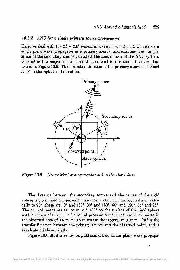
Here, we deal with the 2L — 2M system in a simple sound field, where only asingle plane wave propagates as a primary source, and examine how the po-sition of the secondary source can affect the control area of the ANC system.Geometrical arrangements and coordinates used in this simulation are illus-trated in Figure 10.5. The incoming direction of the primary source is definedas 0° in the right-hand direction.

Primary source

[m]

observ<

observejktrea

Figure 10.5 Geometrical arrangements used in the simulation

x Secondary source

d point

The distance between the secondary source and the centre of the rigidsphere is 0.5 m, and the secondary sources in each pair are located symmetri-cally to 90°, these are: 0° and 180°, 30° and 150°, 60° and 120°, 85° and 95°.The control points are set to 0° and 180° on the surface of the rigid spherewith a radius of 0.08 m. The sound pressure level is calculated at points inthe observed area of 0.6 m by 0.6 m within the interval of 0.02 m. Cpf is thetransfer function between the primary source and the observed point, and itis calculated theoretically.

Figure 10.6 illustrates the original sound field under plane wave propaga-



tion with a frequency of 1 kHz, and Figure 10.3.2 shows noise reduction bythe ANC system with four different arrangements of the secondary sources.To compare these, we take the ratio of the sound pressure level in the originalsound field (i.e. ANC off) and that in the controlled sound field (ANC on)shown in Figure 10.3.2.

-0.3-1

-0.3-0.2-0.1 0 0.1 0.2 0.3x[m]

Figure 10.6 Primary field (0°)

According to the figures, when the incoming direction of the primary sourceagrees with the angle of one of the secondary sources, we can see a largecontrolled area (see Figure 10.3.2d), but Figure 10.3.2a indicates that a closelyplaced secondary sources gives a more significant performance of the noisereduction than wide a arrangement. This can also be seen in Figure 10.3.2.

10.3.3 Diffuse sound field

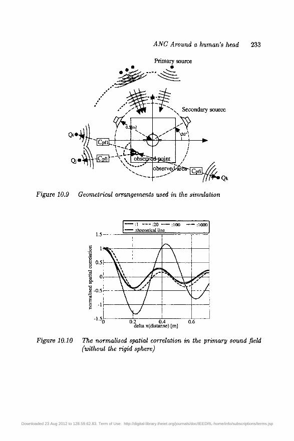
In this Section the diffused sound field is taken into account. Geometricalcoordinates for the diffused field analysis are illustrated in Figure 10.9, and allthe positions of the secondary sources and error microphones are the same asthose for the above discussion (see previous Section). To consider the diffusedsound field, we assume that plane waves come from every direction around thesphere with 5° interval. Thus 72 plane waves with random phase are consideredas the primary sources. The normalised spatial correlation is computed so asto determine the averaging number of the primary sources (see Figures 10.10and 10.11) [163]. We take the average of 100 simulations to calculate the soundpressure level in the diffused condition.

Figure 10.10 shows the normalised spatial correlation in the primary soundfield without a rigid sphere and Figure 10.11 shows the normalised spatial cor-



-0.3-0.2-0.1 0 0.1 0.2 0.3x[m]

-0.3-0.2-0.1 0 0.1 0.2 0.3x[m]

(a) (b)

(c) (d)

Figure 10.7 Controlled area (primary area 0°)

relation with a rigid sphere. Figures 10.12, 10.3.3 and 10.3.3 show the resultsfor the 2L - 2M ANC system. Figures 10.15, 10.3.3 and 10.3.3 present the re-sults for the system with multiple control points on the rigid sphere. Based onthe figures it is obvious that the original sound field is more complicated thanthat due to the single primaxy source (Figure 10.12). However, we can still ob-



SB,

-0.3-0.2-0.1 0 0.1 0.2 0.3x[m]

-0.3-0.2-0.1 0 0.1 0.2 0.3x[m]

-20 -15 -10 -5 0 5 10 15 20 -20 -15 -10 -5 0 5 10 15 20

(a) (b)

-0.3-0.2-0.1 0 0.1 0.2 0.3x[m]

-20 -15 -10 -5 0 5 10 15 20

> • < *

-0.3-0.2-0.1 0 0.1 0.2 0.3x[m]

-20-15-io-5 o s IO 1520

(c) (d)

Figure 10.8 Noise attenuation level (primary area 0°)

serve that an arrangement of closely placed secondary sources (Figure 10.3.3a)gives a large noise reduced area compared to that with wide distances (Fig-ure 10.3.3d). Similar results can also be seen in Figure 10.3.3. Concerning therelationship between the effective area and the number of error microphones,from Figures 10.3.3a and Figure 10.3.36, we can see the very small area with



Primary source

Secondary source

Figure 10.9 Geometrical arrangements used in the simulation

1.5

°-5

"a5

-1.5,

:1 :20 —•• :100 :1000rtheoretical line

\

\\

/

A?J1j

\' /

0.2 0.4 0.6delta x(distanse) [m]

Figure 10.10 The normalised spatial correlation in the primary sound field(without the rigid sphere)



1.5

1

0.5

0

-0.5

-1

- L 5 o

:1 :20 :100 :1000"—— :theoretical line (without the rigid sphere)

-A

0.2 0.4delta x(distanse) [m]

0.6

Figure 10.11 The normalised spatial correlation in the primary soundfieldfwith the rigid sphere)

-0.3-0.3-0.2-0.1 0 0.1 0.2 0.3

x[m]

Figure 10.12 Primary field



-0.3-0.2-0.1 0 0.1 0.2 0.3x[m]

-0.3-0.2-0.1 0 0.1 0.2 0.3x[m]

-60 -55 -50 -45 -40 -35 -30 -25 -20 -60 -55 -50 -45 -40 -35 -30 -25 -20

(a) (b)

l o

-0.3-0.2-0.1 6 0.1 0.2 0.3x[m]

-0.3-0.2-0.1 0 0.1 0.2 03x[m]

-60 -55 -50 -45 -40 -35 -30 -25 -20 -60 -55 -50 -45 -40 -35 -30 -25 -20

(c) (d)

Figure 10.13 Controlled area (secondary sources 85/95°)

large noise reduction level, while some noise attenuation is also observed. Onthe other hand, the multiple-points control system can give a performance



SB,

-0.34-0.3-0.2-0.1 0 0.1 0.2 0.3

x[m]

-0.-0.3-0.2-0.1 0 0.1 0.2 0.3

x[m]

-20 -15 -JO -5 0 5 10 15 20 -20 -15 -10 -5 0 5 10 15 20

(a) (b)

-o.:-0.3

-0.3-0.2-01 0 0 1 0.2 0.3x[m]

- 0 . 3 - 0 . 2 - 0 . 1 0 0 1 0 2 0 .3x[m]

-20 -15 -10 -5 0 5 10 15 20 -20 -15 -10 -5 0 5 10 15 20

(c) (d)

Figure 10.14 Noise attenuation level (secondary sources 85/95°)

with very low noise reduction, although it does not give much noise boost.



-0.3-0.2-0.1 0 0.1 0.2 0.3

x[m]

Figure 10.15 Primary field

10.4 Conclusions

In this Chapter the relationship between noise reduction and the correspond-ing configuration of error microphones and secondary source arrangements hasbeen evaluated using a rigid sphere theoretical model as a human's head. Inthe case of the free sound field, in which the incoming direction of the pri-mary source is known, we found that the arrangement with closely placedsecondary sources has significant performance both for noise reduction as wellas providing a wide control area compared with the distant secondary sourcearrangements. We have shown the results for a primary source of 1 kHz, butit is obvious that more conspicuous results can also be obtained at higherfrequencies. As for the diffused sound field, we confirmed that introducingmultiple control points magnifies the control area of noise reduction but thenoise attenuation level decreases in general. Using our visualisation techniqueof sound pressure around a rigid sphere (as a human head) under control, wealso indicated the possibility of finding the optimal arrangement of the sec-ondary sources and error microphones for a given specification of performancesuch as minimum attenuation level of noise and the shape of the control area.It is by no means easy to settle the matter to the satisfaction of both sides,i.e. wide area and noise reduction level. Genetic algorithms may be employedfor searching the error microphone positions for the purpose of satisfying thepractical specifications which may include the limitation of possible positionsand weighted cost functions for each evaluated position.



-0

-0.3-0.2-0.1 0 0.1 02 03x[m]

-0.3-0.2-0.1 0 0.1 0.2 0.3x[m]

(a) (b)

-0.3-0.2-0.1 0 0 1 0 2 0 3x[m]

-0.3-0.2-0.1 0 0.1 0.2 0.3

(c) (d)

Figure 10.16 Controlled area (secondary sources: 0/18(P)



-0.3--0.3-0.2-0.1 0 0.1 0.2 0.3

x[m]-0.3-0.2-0.1 0 0.1 0.2 0.3

x[m]

-20 -15 -10 -5 0 5 10 15 20 -20 -15 -10 -5 0 5 10 15 20

(a) (b)

-0.3-0.2-0.1 0 0.1 0.2 0.3x[m]

-0.3-0.2-0.1 0 0.1 0.2 0.3x[m]

-20 -15 -10 -5 0 5 10 15 20

(d)

Figure 10.17 Noise attenuation level (secondary sources: 0/18CP)


Active Sound and Vibration Control: theory and applications Volume 25/3 || ANC Around a human's head

Documents

Transcript of Active Sound and Vibration Control: theory and applications Volume 25/3 || ANC Around a human's head