Active Sampling for Class Probability Estimation and...

CeDER Working Paper #IS-01-03, Stern School of Business, New York University, NY, NY 10012

November 7, 2001

Active Sampling for Class Probability Estimation and Ranking

Maytal Saar-Tsechansky [email protected] Department of Information Systems Leonard N. Stern School of Business, New York University 44 West Fourth Street New York, NY 10012, USA Tel: (212) 998-0812 Foster Provost [email protected] Department of Information Systems Leonard N. Stern School of Business, New York University 44 West Fourth Street New York, NY 10012, USA Tel: (212) 998-0806

Abstract

In many cost-sensitive environments class probability estimates are used by deci-sion makers to evaluate the expected utility from a set of alternatives. Supervised learning can be used to build class probability estimates; however, it often is very costly to obtain training data with class labels. Active learning acquires data incre-mentally, at each phase identifying especially useful additional data for labeling, and can be used to economize on examples needed for learning. We outline the critical features for an active learning approach and present an active learning method for estimating class probabilities and ranking. BOOTSTRAP-LV identifies par-ticularly informative new data for learning based on the variance in probability es-timates, and by accounting for a particular data item’s informative value for the rest of the input space. We show empirically that the method reduces the number of data items that must be obtained and labeled, across a wide variety of domains. We investigate the contribution of the components of the algorithm and show that each provides valuable information to help identify informative examples. We also compare BOOTSTRAP-LV with UNCERTAINTY SAMPLING, an existing active learning method designed to maximize classification accuracy. The results show that BOOT-

STRAP-LV uses fewer examples to exhibit a certain class probability estimation accu-racy and provide insights on the behavior of the algorithms. Finally, to further our understanding of the contributions made by the elements of BOOTSTRAP-LV, we ex-periment with a new active learning algorithm drawing from both UNCERTAINTY

SAMPLING and BOOTSTRAP-LV and show that it is significantly more competitive with BOOTSTRAP-LV compared to UNCERTAINTY SAMPLING. The analysis suggests more general implications for improving existing active learning algorithms for classification.

Keyword: Active learning, class probability estimation, cost-sensitive learning

Saar-Tsechansky & Provost

2

1. Introduction Supervised classifier learning requires data with class labels. In many applications, procuring class labels can be costly. For example, to learn diagnostic models experts may need to read many historical cases. To learn document classifiers experts may need read many documents and assign them labels. To learn customer response mod-els, consumers may have to be given costly incentives to reveal their preferences. Active learning processes data incrementally, using the model learned "so far" to select particularly helpful additional training examples for labeling. When successful, active learning methods reduce the number of instances that must be labeled to achieve a particular level of accuracy. Most existing methods and particularly empiri-cal approaches for active learning address classification problems—they assume the task is to assign cases to one of a fixed number of classes. Many applications, however, require more then simple classification. In particular, probability estimates are central in decision theory, allowing a decision maker to in-corporate costs/benefits for evaluating alternatives. For example, in target marketing the estimated probability that a customer will respond to an offer is combined with the estimated profit (Zadrozny and Elkan, 2001) to evaluate various offer proposi-tions. Other applications require ranking of cases, to improve consumer response rate to offer propositions, as well as to add flexibility for user processing1. For example, documents can be ranked by their probability of being of interest to the user, and offers to consumers may be presented/proposed in order of the probability of pur-chase or of the expected benefit to the seller. We therefore focus on learning class probability estimation (CPE) models.

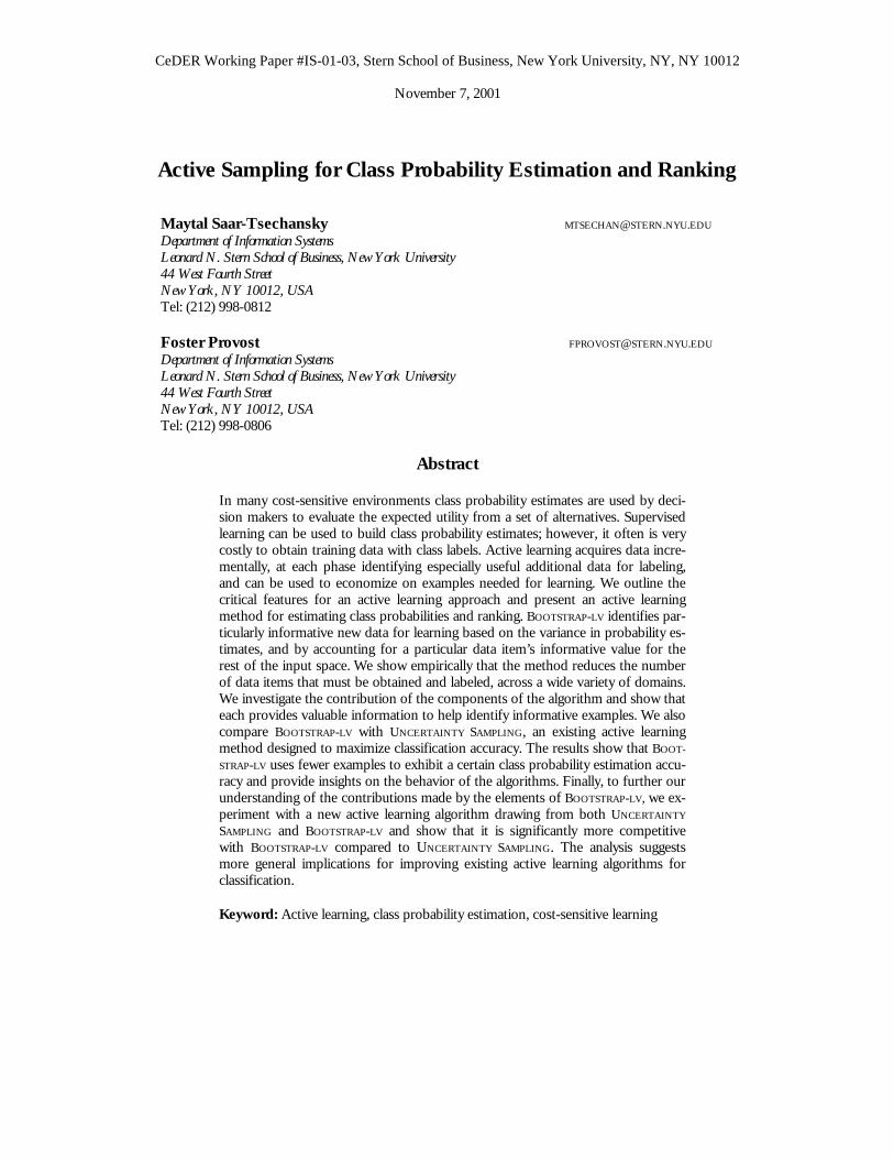
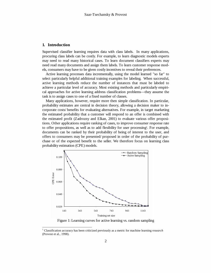
Figure 1: Learning curves for active learning vs. random sampling

1 Classification accuracy has been criticized previously as a metric for machine learning research (Provost et al., 1998).

0.029

0.049

0.069

0.089

0.109

143 343 543 743 943 1143

Training set size

CPE

Erro

r

Random SamplingActive Sampling


3

In this paper we consider active learning to produce accurate CPEs and class-based rankings from fewer learning examples. Figure 1 shows the desired behavior of an active learner. The horizontal axis represents the information needed for learning, i.e., the number of training examples, and the vertical axis represents the error rate of the probabilities produced by the learned model. Each learning curve shows how error rate decreases as more training data are used. The upper curve represents the de-crease in error from randomly selecting training data; the lower curve represents ac-tive learning. The two curves form a "banana" shape: very early on, the curves are comparable because a model is not yet available for active learning. The active learn-ing curve soon accelerates, because of the careful choice of training data. Given enough data, random selection catches up. We introduce a new active learning technique, BOOTSTRAP-LV, for learning CPEs. BOOTSTRAP-LV uses bootstrap samples (Efron and Tibshirani, 1993) of available training data to examine the variance in the probability estimates for not-yet-labeled data, and employs a weight sampling procedure to finally select particularly informative exam-ple for learning. We show empirically across a wide range of data sets that BOOTSTRAP-LV decreases the number of labeled instances needed to achieve accurate probability estimates, or alternatively that it increases the accuracy of the probability estimates for a fixed number of training data. A careful analysis of the algorithm’s characteristics and performance reveals the contributions of its components. The analysis also leads to a new algorithm for active learning that is more competitive compared to other methods with respect to BOOTSTRAP-LV and has computational advantages. The latter further demonstrates how the components of the BOOTSTRAP-LV algorithm contribute to its efficacy and highlights why existing algorithms do not perform well for CPE.

2. Active Learning and the Bootstrap-LV Algorithm

The fundamental notion of active learning has a long history in machine learning. To our knowledge, the first to discuss it explicitly were (Simon and Lea, 1974) and (Winston, 1975). Simon and Lea describe how machine learning is different from other types of problem solving, because learning involves the simultaneous search of two spaces: the hypothesis space and the instance space. The results of searching the hypothesis space can affect how the instance space will be sampled. Winston dis-cusses how the best examples to select next for learning are "near misses," instances that miss being class members for only a few reasons. Subsequently, theoretical re-sults showed that the number of training data can be reduced substantially if they can be selected carefully (Angluin, 1988). The term active learning was coined later to de-scribe induction where the algorithm controls the selection of potential unlabeled training examples (Cohn et al., 1994). A generic algorithm for active learning is shown in Figure 2. A learner first is ap-plied to an initial set L of labeled examples (usually selected at random or provided by an expert). Subsequently, sets of M examples are selected in phases from a set of unlabeled examples UL, until some predefined condition is met (e.g., the labeling budget is exhausted). In each phase, each candidate example ULxi ∈ is assigned an


4

effectiveness score iES based on an objective function, reflecting its contribution to subsequent learning. Examples then are selected for labeling based on their effective-ness scores. Often, multiple examples, rather than a single example, are selected in each phase due to computational constraints. Once examples are selected, their labels are obtained (e.g., by querying an expert) before being added to L, to which the learner is applied next.

Input: an initial labeled set L, an unlabeled set UL, an inducer I, a stopping criterion, and an integer M specifying the number of actively selected exam-ples in each phase.

1 While stopping criterion not met /* perform next phase: */ 2 Apply inducer I to L 3 For each example { ULxx ii ∈| } compute iES , the effectiveness score 4 Select a subset S of size M from UL based on iES 5 Remove S from UL, label examples in S, and add S to L Output: estimator E induced with I from the final labeled set L

Figure 2: Generic Active Learning Algorithm The objective of active learning is to select examples that will reduce the generaliza-tion error of the model the most. The generalization error is the expected error across the entire example space. Therefore when evaluating a learning example an optimal active learning approach must evaluate the expected reduction in generalization error if the example were to be added to the training set from which the model would be induced. The example that is expected to reduce the generalization error the most should be added to the training set. We are interested in an active learning scheme that will apply to arbitrary learners, thus computational considerations may prohibit us from examining the models re-sulting from adding each potential unlabeled example to the training set (as pre-scribed by Roy and McCallum (Roy and McCallum, 2001). We therefore resort to an indirect estimation of potential learning examples’ informative value. Also, we con-sider the potential of each learning example to help improve the estimation of other examples in the space not only the performance of its own class probability, which we describe in detail below. Given the generic framework presented in Figure 2, BOOTSTRAP-LV embodies a par-ticular instantiation of steps 3 and 4. The description we provide here pertains to binary classification problems. Since our goal is to reduce the class probability estimation (CPE) error, it is useful to understand its sources. A model’s estimation )|(ˆ Txf for a particular input x de-pends upon the sample T from which the model is induced, and therefore can be treated as a random variable. Let )(xf be the underlying function describing the probability of class membership for a case described by input x. One indication of the quality of the current class probability estimate )|(ˆ Txf for example x given a training


5

set T is the expected estimation (absolute) error, reflecting the discrepancy between the estimated probability and the true probability, i.e., |)|(ˆ)(| Txfxf − . We may infer from the discrepancy whether additional information is needed to improve the model’s estimation. Note however, that in an inductive learning setting the class prob-ability for an input, )(xf , is not known to us, even when an instance’s true class is known. A common formulation of the estimation error (Friedman, 1997) decomposes the expected squared estimation error into the sum of two terms:

222 )]|(ˆ)([)]|(ˆ)|(ˆ[)]|(ˆ)([( TxfExfTxfETxfETxfxfE TTTT −+−=− , )(⋅E represents expectation across training sets T. The first term in the sum is re-

ferred to as the “variance” of the estimation and reflects the sensitivity of the estima-tion to the training sample. The second term is referred to as the (squared) “bias”, reflecting the extent to which the induced model can approximate the target function

)(xf (Friedman, 1997). Both the estimation error and the estimation bias refer to the actual probability function, )(xf , which as mentioned is not available for an induc-tive learning algorithm to consider. Therefore it is impossible to compute them di-rectly. The estimation “variance”, however, reflects a behavior of the estimation procedure without reference to the underlying probability function. In order to reduce the estimation error the BOOTSTRAP-LV algorithm estimates and then tries to reduce the estimation variance. The estimation variance for a certain input is referred to as the “local variance” (LV) to differentiate it from the model’s expected variance over the entire input space. We ignore the bias, or alternatively assume the bias is zero. The BOOTSTRAP-LV algorithm, shown in Figure 3, first estimates the estimation vari-ance of each potential learning example (the LV). If the LV is high, we infer that this example is not well captured by the model given the available data. The local variance also reflects the potential error reduction if this variance were reduced as more exam-ples become available for the learner. BOOTSTRAP-LV then employs the LV estimations together with a specialized sampling procedure to identify the examples that are par-ticularly likely to reduce the average estimation error across the entire example space (i.e., generalization error) the most. We first describe the estimation of the estimation variance. We then will discuss the sampling procedure.

Given that an efficient closed-form estimation of the local variance may not be ob-tained for arbitrary learners, we estimate it empirically. The variance stems from the estimation being induced from a random sample. We therefore emulate a series of samples by generating a set of k bootstrap subsamples (Efron and Tibshirani, 1993)

jB , kj ,...,1= from L. We generate a set of models by applying the inducer I to each bootstrap sample jB , resulting in k estimators jE , kj ,...,1= . To calculate the esti-mated variance, for each example in ULxi ∈ , we estimate the variance among CPEs predicted by the estimators {

jE }. Finally, each example in ULxi ∈ is assigned an effectiveness score that is proportional to its local variance.


6

Algorithm BOOTSTRAP-LV Input: an initial labeled set L sampled at random, an unlabeled set UL, an inducer I , a stop-ping criterion, and a sample size M. 2 for (s=1;until stopping criterion is met; s++) 3 Generate k bootstrap subsamples

jB , kj ,...,1= from L 4 Apply inducer I on each subsample

jB and induce estimator jE

5 For all examples { ULxx ii ∈| } compute ( ){ }R

ppxpxD

ik

j iijis

min,12)(

)(∑=

−=

6 Sample from the probability distribution sD , a subset S of M examples from UL with-out replacement

7 Remove S from UL, label examples in S, and add them to L 8 end for Output: estimator E induced with I from L

Figure 3: The BOOTSTRAP-LV Algorithm The local variance provides an indication of the potential error reduction for each

individual example in the example space if more relevant examples are provided to the learner. It does not however provide an indication of how much is learned from each learning example about other examples in the space. We stated earlier that our objective is to reduce the generalization error by training a model with fewer, particu-larly informative examples, and we emphasized the potential impact a learning exam-ple may have on reducing the estimation error of other examples in the example space. Consider an active learning algorithm where the effectiveness score reflects the potential contribution of a learning example to reducing its own error. Also assume examples are selected in order of their effectiveness score, such that the examples with the highest scores are selected for labeling first. We refer to this approach as Direct Selection. Direct selection ignores information about how the class probability estimation error of other examples in the space may be affected by adding an example to the training set. The latter, however, is essential to evaluate the expected effect an example may have on the generalization error.

Random sampling is often referred to in the active learning literature as non-informed learning (e.g., (Cohn et al., 1994, Lewis and Gale, 1994)). Nevertheless, random sampling is powerful because it allows the incorporation of information about the distribution of examples even when the information is not known explic-itly. For example, consider the case when examples for labeling are sampled at ran-dom. An example may inform the learning about other examples in the space if it shares some common features with these examples. Consider a set of examples shar-ing a set of features. With random sampling, the larger this set the more likely it is that an example from this set is sampled, providing information about a larger num-ber of examples. Note that this property is obtained without having to capture explic-itly how examples are associated with each other.


7

In order to reduce the average error across the example space BOOTSTRAP-LV incor-porates sampling into the selection of training examples by weight sampling examples for labeling. In particular, the probability of each example to be sampled is propor-tional to its local variance.

Specifically, the distribution from which examples are sampled is given by ( ){ }

R

ppxpxD

ik

j iijis

min,12)(

)(∑ =

−= , where )( ij xp denotes the estimated probability an estima-

tor jE assigns to the event that example ix belongs to one of the two classes (the choice of performing the calculation for either class is arbitrary because the variance for both classes is equal); ip =

k

xpk

j ij∑ =1)( ; min,ip is the average probability estimation

assigned to the minority class by the estimators {jE } , and R is a normalizing factor

( ){ }∑ ∑= =−= )(

1 min,12)(ULsize

i ik

j iij ppxpR , so that sD is a distribution.

There is one additional technical point of note. Consider the case where the classes are not represented equally in the training data. When high variance exists in regions of the domain for which the minority class is assigned high probability, it is likely that the region is relatively better understood than regions with the same variance but for which the majority class is assigned high probability. In the latter case, the class prob-ability estimation may be exhibiting high variance due simply to lack of representation of the minority class in the training data, and would benefit from sampling more in the respected region. Therefore the estimated variance is divided by the average value of the minority-class probability estimates min,ip . The minority class is determined once from the initial random sample.

3. Related Work

Cohn et al. (Cohn et al., 1996) propose an active learning approach for statistical learning models, generating queries (i.e., learning examples) from the input space to be used as inputs to the learning algorithm. This approach directly evaluates the effec-tiveness score, i.e., the informative contribution of each example to the learning task. At each phase the expectation of the variance of the model over the example space is used to generate the example that minimizes this variance. Since it requires a compu-tation in closed form of the learner’s variance, this approach is impracticable for arbi-trary models. In addition, queries are generated whereas here we are interested in identifying informative examples from an existing set of available unlabeled examples (a subset of the set of possible queries). When an efficient closed-form estimation of the expected generalization error is not available, the models that result from adding each potential learning example to the training set can be induced in order to estimate the expected changes in generali-zation error. Roy and McCallum (Roy and McCallum, 2001) propose this approach for building classifiers. At each phase they update the current model with each addi-tional learning example for each possible label and calculate an effectiveness score, measured as class entropy, as an estimate of the improvement in classification error.


8

They then select the example bringing about the greatest expected reduction of en-tropy. The algorithm was shown to be effective, reducing the number of examples needed to obtain a certain level of accuracy. For many learning algorithms, however, the induction of a new model for each possible training example may be prohibitively expensive. A critical requirement for their approach, therefore, allowing it to be com-putationally tractable, is that the learning algorithm allows efficient incremental up-dates of the model, such as the Naïve Bayes algorithm used to classify text documents in the paper (Roy and McCallum, 2001). When an efficient closed-form computation of the error or incremental model updates are not possible, various active learning approaches compute alternative ef-fectiveness scores. In particular, the QUERY BY COMMITTEE (QBC) algorithm (Seung et al.,1992) was proposed to select learning examples actively for training a binary classi-fier. Examples are sampled at random, generating a “stream” of potential learning examples, and each example is considered informative (and thus is labeled) if classifi-ers sampled from the current version space disagree regarding its class prediction. The QBC algorithm employs disagreement as a binary effectiveness score, designed to capture whether or not uncertainty exists regarding class prediction given the cur-rent labeled examples. McCallum and Nigam (McCallum and Nigam, 1998) note that a disadvantage of the “stream-based” QBC approach lies in the decision of whether to label an example being “made on each document (i.e., example) individually, irrespective of the alterna-tives”. Alternatively, estimation uncertainty of all the unlabeled learning examples can be compared, allowing one to select at each phase the example(s) with the largest classification uncertainty. Various other approaches have been developed within the Query By Committee framework that identify informative examples for constructing classifiers and which use a variety of measures that quantify the level of uncertainty or the likelihood of classification error given the current labeled data. In particular, these effectiveness scores quantify the estimated informative value of each example to ob-tain a ranking of the examples’ informative values. Subsequently the example(s) with the highest effectiveness score(s) is (are) selected. For instance, Abe and Mamimtsuka (Abe and Mamimtsuka, 1998) use bagging and boosting to generate a committee of classifiers and quantify disagreement as the mar-gin (i.e., the difference in weight assigned to either class). Examples with the mini-mum margin are selected for labeling. The final classifier is composed of an ensemble of classifiers whose votes are used for class prediction. UNCERTAINTY SAMPLING (Lewis and Gale, 1994) was designed to select informative examples to construct binary clas-sifiers by adopting the uncertainty notion underlying the QBC approach, but instead of generating a committee of hypotheses to estimate uncertainty the algorithm em-ploys a single probabilistic classifier. Examples whose probabilities of class member-ship are closest to 0.5 are selected for labeling first. UNCERTAINTY SAMPLING has several attractive properties that we return to below. All these methods, as indicated by their effectiveness scores, are designed to in-crease classification accuracy, not to improve CPEs or rankings, which is our concern in this paper. In addition, differently from the approach we propose in this paper


9

these methods do not incorporate the effect of a learning example on other examples across the example space. Particularly, they disregard the potential effect of a training example on reducing the error of other examples in the example space. Examples for which the current estimation is most uncertain may have no significant contribution to reducing the estimation error of other examples in the instance space. The failure to account for this effect was noted by Dagan and Engelson (Dagan and Engelson, 1999) as well as by McCallum and Nigam (McCallum and Nigam, 1998) who pro-posed to incorporate an instance density measure explicitly into the effectiveness score, where the density measure reflects how similar are other examples in the space to the one examined. The underlying assumption is that the proposed similarity measure captures the relative effect an example would have on reducing the classifica-tion error of other examples in the space. The approach was shown to be effective in selecting informative examples for document classification. Yet the proposed density measure is specific to document items, where similarity measures are available (e.g., TF/IDF). It is not clear what an appropriate density measure may be for an arbitrary domain2.

Our approach uses weight sampling, by which we argue it implicitly incorporates properties of the domain to support the selection of examples more likely to be in-formative regarding other examples in the space. Note that weight sampling also is employed in the AdaBoost algorithm (Freund and Shapire, 1996) on which Iyengar et al. (Iyengar et al., 2000) base their active learning approach. Their algorithm results in an ensemble of classifiers where weight sampling is used both to select examples from which successive classifiers in the ensemble are generated as well as to select examples for labeling. Iyengar et. al note that better results were obtained when ex-amples were sampled compared to when examples are selected by order of their error measure. They propose to study this phenomenon further and hypothesize that sam-pling allows their approach to avoid selecting the same examples repeatedly. How-ever, we argue that in addition weight sampling acts to increase the likelihood of selecting examples that are particularly informative for reducing the generalization error. As we discuss in the previous paragraph, selecting examples should address the relevance of each learning example to other examples in order to identify examples that will better decrease the average estimation error (i.e., the generalization error). Moreover, whereas the domain-specific approach of McCallum and Nigam modeled the example space explicitly and incorporated a measure of space density into the effectiveness score (McCallum and Nigam, 1998), the weight-sampling mechanism can be applied seamlessly for arbitrary domains.

In sum, BOOTSTRAP-LV employs an effectiveness score which identifies examples whose CPE varies highly. It uses this measure to indicate the potential improvement in class probability estimation error, rather than classification accuracy. BOOTSTRAP-LV estimates local variance empirically, enabling its computation with an arbitrary model-ing scheme. Lastly, we use a sampling mechanism to complement the selection of 2 Roy and McCallum note the domain-specific limitation of this approach [Roy and McCallum,

2001].


10

examples for learning. We argue that weight sampling can help account for the in-formative value an example confers for other examples in the space.

4. Experimental Evaluation

The experiments we describe here examine BOOTSTRAP-LV’s performance over a range of domains in order to assess its general ability to identify particularly useful examples for learning. In section 4.1 we present our experimental setting. Sections 4.2 and 4.3 present and discuss our results with simple probability estimation trees, and with bagged probability estimation trees, respectively. We discuss addition evaluation measures in section 4.4. In Section 4.5 we compare BOOTSTRAP-LV with UNCERTAINTY

SAMPLING, an active learning approach for classifiers, to provide insights on the opera-tion of the algorithm and its advantage compared to existing approaches. Finally, experiments with a new active learning algorithm inspired by the empirical investiga-tion provide further insights into the elements of the BOOTSTRAP-LV algorithm.

4.1 Experimental Setting We applied BOOTSTRAP-LV to 20 data sets, 17 from the UCI machine learning reposi-

tory (Blake et al., 1998) and 3 used previously to evaluate rule-learning algorithms (Cohen and Singer, 1999). Data sets with more than two classes were mapped into two-class problems.

For these experiments we use tree induction to produce class probability esti-mates2. In particular, for the experiments presented here, the underlying probability estimator is a Probability Estimation Tree (PET), an unpruned C4.5 decision tree (Quinlan, 1993) for which the Laplace correction (Cestnik, 1990) is applied at the leaves. Not pruning and using the Laplace correction had been shown to improve the CPEs produced by PETs (Bauer and Kohavi, 1999; Provost et al., 1998; Provost & Domingos, 2000; Perlich et al. 2001).

To evaluate the predictive quality of the CPE models induced by BOOTSTRAP-LV it would be desirable to compare against the true class probability values, for example, computing the mean absolute error with respect to the actual probabilities. However, in these data sets only class membership is observed and the true class probabilities are unknown. As models are learned from more data, performance improves typically as a learning curve; BOOTSTRAP-LV aims to obtain comparable performance with fewer labeled data (recall figure 1). We compare the probabilities assigned by the model induced with BOOTSTRAP-LV at each phase with those assigned by a “best” estimator,

BE , as surrogates to the true probabilities, where BE is induced from the entire set of available learning examples ULL ∪ (where the labels of all examples are known to us). In particular, we induce BE using bagged PETs, which have shown to produce superior probability estimates compared to individual PETs (Bauer and Kohavi, 1999; Provost et al., 1998; Provost & Domingos, 2000). We then calculate the mean abso- 2 Probability estimation trees are easy to build, fast computationally, robust across data sets, comprehensible to human experts, and produces surprisingly good probability-based rankings [Perlich et al., 2001]


11

lute error, denoted BMAE (Best-estimate Mean Absolute Error), for an estimator E

with respect to BE 's estimation. BMAE is given by N

xpxpBMAE

N

i iEiEB∑=−

= 1)()( , where

)( iE xpB

is the estimated probability given by BE ; )( iE xp is the probability estimated by E, and N is the number of (test) examples examined.

We compare the performance of BOOTSTRAP-LV with a method, denoted by RANDOM, where estimators are induced with the same inducer and the same training-set size, but for which examples are sampled at random. We compare across different sizes of the labeled set L. In order not have very large sample sizes, M, for large data sets and very small ones for small data sets, we applied different numbers of sampling phases for different data sets, varying between 10 and 30; at each phase the same number of examples was added to L. Results are averaged over 10 random, three-way partitions of the data sets into an initial labeled set, an unlabeled set, and a test set against which the two estimators are evaluated. For control the same partitions were used by both RANDOM and BOOTSTRAP-LV.

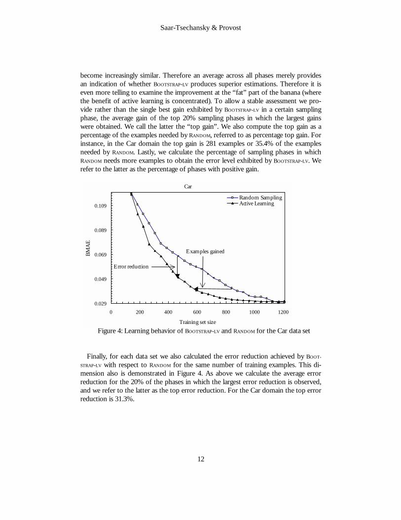
The banana curve in Figure 4 shows the relative performance for the Car data set. As shown in Figure 4, the error of the estimator induced with BOOTSTRAP-LV decreases faster initially, exhibiting lower error for fewer examples. This demonstrates that ex-amples actively added to the labeled set are more informative (on average), allowing the inducer to construct a better estimator for a certain number of learning examples. Note that for visibility the algorithms’ performance with the initial labeled set (for which all algorithms perform identically) is not shown.

Evaluations of active learning algorithms often present only the initial part of the learning curve to demonstrate the efficacy of the algorithm. We summarize the com-parative performance of the competing algorithms also across the entire leaning curve. In particular, the objective of BOOTSTRAP-LV is to enable learning with fewer examples in order to obtain a certain level of CPE accuracy. For each data set we calculate a set of measures pertaining to the gain obtained with BOOTSTRAP-LV in terms of the number of examples that did not need to be labeled when using BOOTSTRAP-LV instead of RANDOM. The number of examples gained for a certain performance level is demonstrated in Figure 4. For each sampling phase of the algorithm we calculate the difference in the number of examples needed by BOOTSTRAP-LV to obtain the exhibited error level and the number needed by RANDOM to obtain the same error level. We calculate the average gain across all sampling phases, referred to as average gain, as well as the gain as a percentage of the number of examples needed by RANDOM (i.e., the percentage of examples gained if BOOTSTRAP-LV is used instead of RANDOM), referred to as average percentage gain. For instance, in the Car domain (Figure 4) the average gain is 155 examples and the average percentage gain is 23.3% of the examples needed by RANDOM.

Because of the natural banana shape of the learning curves, even for the ideal case the performance of estimators induced from any two samples cannot be considerably different at the final sampling phases, as most of the available examples have been used by both sampling methods and therefore the samples obtained by the methods


12

become increasingly similar. Therefore an average across all phases merely provides an indication of whether BOOTSTRAP-LV produces superior estimations. Therefore it is even more telling to examine the improvement at the “fat” part of the banana (where the benefit of active learning is concentrated). To allow a stable assessment we pro-vide rather than the single best gain exhibited by BOOTSTRAP-LV in a certain sampling phase, the average gain of the top 20% sampling phases in which the largest gains were obtained. We call the latter the “top gain”. We also compute the top gain as a percentage of the examples needed by RANDOM, referred to as percentage top gain. For instance, in the Car domain the top gain is 281 examples or 35.4% of the examples needed by RANDOM. Lastly, we calculate the percentage of sampling phases in which RANDOM needs more examples to obtain the error level exhibited by BOOTSTRAP-LV. We refer to the latter as the percentage of phases with positive gain.

Figure 4: Learning behavior of BOOTSTRAP-LV and RANDOM for the Car data set Finally, for each data set we also calculated the error reduction achieved by BOOT-

STRAP-LV with respect to RANDOM for the same number of training examples. This di-mension also is demonstrated in Figure 4. As above we calculate the average error reduction for the 20% of the phases in which the largest error reduction is observed, and we refer to the latter as the top error reduction. For the Car domain the top error reduction is 31.3%.

Car

0.029

0.049

0.069

0.089

0.109

0 200 400 600 800 1000 1200

Training set size

BMA

E

Random SamplingActive Learning

Examples gained

Error reduction


13

4.2 Results: Bootstrap-LV versus Random Sampling

For some data sets BOOTSTRAP-LV exhibits even more dramatic results than those presented for the Car data set above; Figure 5 shows results for the Pendigits data set (the most impressive “win”). BOOTSTRAP-LV achieves its almost minimal level of error at about 4000 examples. RANDOM requires more than 9300 examples to obtain this error level. It is important to note that an active learning algorithm’s performance is par-ticularly interesting in the initial sampling phases demonstrating the performance that can be obtained for a relatively small portion of the data and therefore a small labeling cost. As can be seen in Figure 4, in the initial phases the error exhibited by the model induced from BOOTSTRAP-LV’s selection of learning examples is reduced substantially faster than when examples are sampled randomly.

Figure 5: CPE learning curves for the Pendigits data set. BOOTSTRAP-LV accelerates error

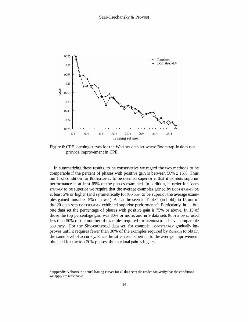
reduction considerable in the initial sampling phases. For 5 of the 20 data sets, BOOTSTRAP-LV did not succeed in accelerating learning

much or at all, as is shown for the Weather data set in Figure 6. Note that the accu-racy was comparable to that obtained with random sampling, as neither curve consis-tently resides above the other. This is discussed further below.

Table 1 presents a summary of our results for all the data sets. The second column shows the percentage of phases with positive gain. The third and fourth columns show the top percentage gain and the top gain (respectively). The fifth and sixth col-umns of Table 1 show the average percentage gain and the average gain across all sampling phases by applying BOOTSTRAP-LV. The seventh Column presents the top error reduction.

0.0165

0.0215

0.0265

0.0315

0.0365

0.0415

0.0465

352 2352 4352 6352 8352Training set size

BMA

E

RandomBootstrap-LV


14

Figure 6: CPE learning curves for the Weather data set where Bootstrap-lv does not

provide improvement in CPE

In summarizing these results, to be conservative we regard the two methods to be comparable if the percent of phases with positive gain is between 50% ± 15%. Thus our first condition for BOOTSTRAP-LV to be deemed superior is that it exhibits superior performance in at least 65% of the phases examined. In addition, in order for BOOT-

STRAP-LV to be superior we require that the average examples gained by BOOTSTRAP-LV be at least 5% or higher (and symmetrically for RANDOM to be superior the average exam-ples gained must be –5% or lower). As can be seen in Table 1 (in bold), in 15 out of the 20 data sets BOOTSTRAP-LV exhibited superior performance3. Particularly, in all but one data set the percentage of phases with positive gain is 75% or above. In 13 of those the top percentage gain was 30% or more, and in 9 data sets BOOTSTRAP-LV used less than 50% of the number of examples required for RANDOM to achieve comparable accuracy. For the Sick-euthyroid data set, for example, BOOTSTRAP-LV gradually im-proves until it requires fewer than 30% of the examples required by RANDOM to obtain the same level of accuracy. Since the latter results pertain to the average improvement obtained for the top-20% phases, the maximal gain is higher.

3 Appendix A shows the actual leaning curves for all data sets; the reader can verify that the conditions we apply are reasonable.

0.235

0.24

0.245

0.25

0.255

0.26

0.265

0.27

0.275

174 674 1174 1674 2174 2674 3174 3674Training set size

BMA

ERandomBootstrap-LV


15

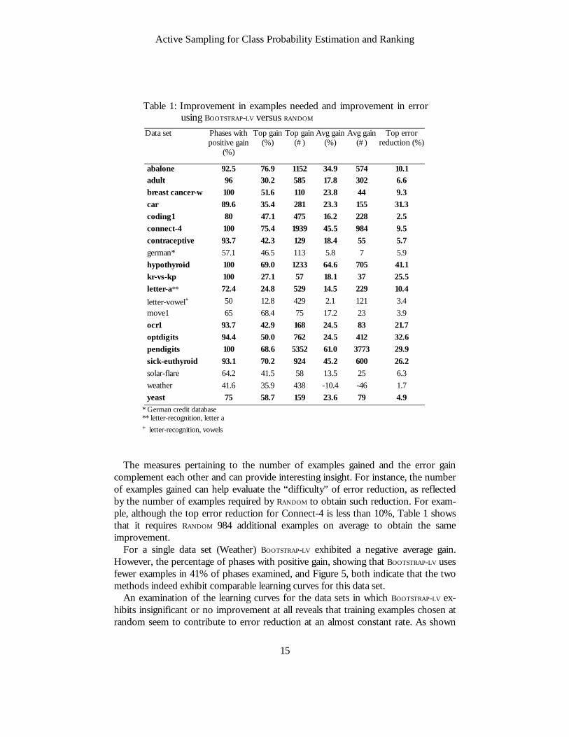
Table 1: Improvement in examples needed and improvement in error using BOOTSTRAP-LV versus RANDOM

Data set

Phases with positive gain

(%)

Top gain (%)

Top gain (#)

Avg gain (%)

Avg gain (#)

Top error reduction (%)

abalone 92.5 76.9 1152 34.9 574 10.1 adult 96 30.2 585 17.8 302 6.6 breast cancer-w 100 51.6 110 23.8 44 9.3 car 89.6 35.4 281 23.3 155 31.3 coding1 80 47.1 475 16.2 228 2.5 connect-4 100 75.4 1939 45.5 984 9.5 contraceptive 93.7 42.3 129 18.4 55 5.7 german* 57.1 46.5 113 5.8 7 5.9 hypothyroid 100 69.0 1233 64.6 705 41.1 kr-vs-kp 100 27.1 57 18.1 37 25.5 letter-a** 72.4 24.8 529 14.5 229 10.4 letter-vowel+ 50 12.8 429 2.1 121 3.4 move1 65 68.4 75 17.2 23 3.9 ocr1 93.7 42.9 168 24.5 83 21.7 optdigits 94.4 50.0 762 24.5 412 32.6 pendigits 100 68.6 5352 61.0 3773 29.9 sick-euthyroid 93.1 70.2 924 45.2 600 26.2 solar-flare 64.2 41.5 58 13.5 25 6.3 weather 41.6 35.9 438 -10.4 -46 1.7 yeast 75 58.7 159 23.6 79 4.9

* German credit database ** letter-recognition, letter a + letter-recognition, vowels

The measures pertaining to the number of examples gained and the error gain

complement each other and can provide interesting insight. For instance, the number of examples gained can help evaluate the “difficulty” of error reduction, as reflected by the number of examples required by RANDOM to obtain such reduction. For exam-ple, although the top error reduction for Connect-4 is less than 10%, Table 1 shows that it requires RANDOM 984 additional examples on average to obtain the same improvement.

For a single data set (Weather) BOOTSTRAP-LV exhibited a negative average gain. However, the percentage of phases with positive gain, showing that BOOTSTRAP-LV uses fewer examples in 41% of phases examined, and Figure 5, both indicate that the two methods indeed exhibit comparable learning curves for this data set.

An examination of the learning curves for the data sets in which BOOTSTRAP-LV ex-hibits insignificant or no improvement at all reveals that training examples chosen at random seem to contribute to error reduction at an almost constant rate. As shown


16

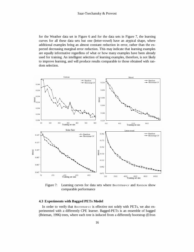
for the Weather data set in Figure 6 and for the data sets in Figure 7, the learning curves for all these data sets but one (letter-vowel) have an atypical shape, where additional examples bring an almost constant reduction in error, rather than the ex-pected decreasing marginal error reduction. This may indicate that learning examples are equally informative regardless of what or how many examples have been already used for training. An intelligent selection of learning examples, therefore, is not likely to improve learning, and will produce results comparable to those obtained with ran-dom selection.

Figure 7: Learning curves for data sets where BOOTSTRAP-LV and RANDOM show comparable performance

4.3 Experiments with Bagged PETs Model In order to verify that BOOTSTRAP-LV is effective not solely with PETs, we also ex-perimented with a differently CPE learner. Bagged-PETs is an ensemble of bagged (Brieman, 1996) trees, where each tree is induced from a differently bootstrap (Efron

German

0.184

0.194

0.204

0.214

0.224

0.234

0.244

63 163 263 363 463 563 663Training set size

BMA

E

RandomBootstrap-LV

Move1

0.124

0.144

0.164

0.184

0.204

0.224

112 612 1112 1612Training set size

BMA

E

RandomBootstrap-LV

Solar-flare

0.047

0.067

0.087

0.107

0.127

0.147


BMA

E

RandomBootstrap-LV

Letter-vowel

0.072

0.092

0.112

0.132

0.152

0.172

0.192

522 2522 4522 6522 8522 10522Training set size

BMA

E

RandomBootstrap-LV


17

and Tibshirani, 1993) sample. The trees are used to estimate the class probability of an instance by averaging the CPEs of the PETs in the ensemble. Bagged-PETs are not comprehensible models, but have been shown generally to produce superior CPEs compared to single PETs (Bauer and Kohavi, 1999; Provost et al., 1998; Pro-vost & Domingos, 2000).

BOOTSTRAP-LV’s performance for the bagged-PETs model concurs with the results obtained for individual PETs. Particularly, for 15 of the data sets BOOTSTRAP-LV exhib-ited phases-gained of more than 65% (in 13 of those phases-gained is more than 75%). The average of the top-20% example gain was 25% or higher in 11 of those data sets. Only in two data sets is phases-gained less than 40%.

Figure 8 shows a comparison between BOOTSTRAP-LV and RANDOM for individual PETs and for bagged-PETs. The overall error exhibited by the bagged-PETs is lower than for the PET, and for both models BOOTSTRAP-LV achieves its lowest error with considerably fewer examples than are required for RANDOM.

Figure 8: CPE learning curves for the Hypothyroid data set showing performance for BOOTSTRAP-LV and RANDOM with bagged PETs and single PETs.

4.4 Other Evaluation Criteria We also evaluated BOOTSTRAP-LV using alternative performance measures: the 0/1

mean squared error measure used by Bauer and Kohavi (1999), as well as the area under the ROC curve (denoted AUC) (Bradley 1997), which specifically evaluates ranking accuracy.

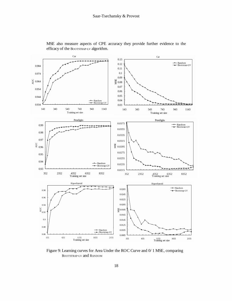
The results for these measures agree with those obtained with BMAE. For exam-ple, BOOTSTRAP-LV generally leads to fatter ROC curves with fewer examples. Figure 9 presents learning curves of both measures for the Car and Pendigits and Hypothyroid data sets, whose learning curves using BMAE were presented earlier. As AUC and

0.005

0.01

0.015

0.02

0.025

0.03

0.035


BMA

E

BPET RandomBPET Bootstrap-LVPET RandomPET Bootstrap-LV


18

MSE also measure aspects of CPE accuracy they provide further evidence to the efficacy of the BOOTSTRAP-LV algorithm.

Figure 9: Learning curves for Area Under the ROC Curve and 0/1 MSE, comparing BOOTSTRAP-LV and RANDOM

Pendigits

0.93

0.94

0.95

0.96

0.97

0.98

0.99


AU

C

RandomBootsrap-LV

Pendigits

0.0215

0.0235

0.0255

0.0275

0.0295

0.0315

0.0335

0.0355

0.0375


MSE

RandomBootsrap-LV

Hypothyroid

0.86

0.88

0.9

0.92

0.94

0.96

0.98


AU

C

RandomBootstrap-LV

Hypothyroid

0.0085

0.0105

0.0125

0.0145

0.0165

0.0185

0.0205

0.0225

0.0245

0.0265


MSE

RandomBootstrap-LV

Car

0.934

0.944

0.954

0.964

0.974

0.984


AU

C

RandomBootstrap-LV

Car

0.03

0.040.05

0.060.07

0.08

0.090.1

0.110.12

0.13


MSE

RandomBootstrap-LV


19

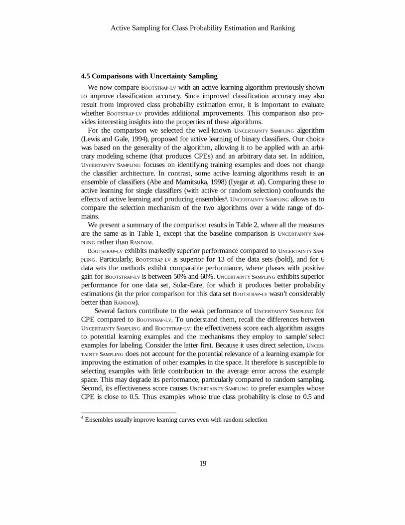
4.5 Comparisons with Uncertainty Sampling We now compare BOOTSTRAP-LV with an active learning algorithm previously shown

to improve classification accuracy. Since improved classification accuracy may also result from improved class probability estimation error, it is important to evaluate whether BOOTSTRAP-LV provides additional improvements. This comparison also pro-vides interesting insights into the properties of these algorithms. For the comparison we selected the well-known UNCERTAINTY SAMPLING algorithm (Lewis and Gale, 1994), proposed for active learning of binary classifiers. Our choice was based on the generality of the algorithm, allowing it to be applied with an arbi-trary modeling scheme (that produces CPEs) and an arbitrary data set. In addition, UNCERTAINTY SAMPLING focuses on identifying training examples and does not change the classifier architecture. In contrast, some active learning algorithms result in an ensemble of classifiers (Abe and Mamitsuka, 1998) (Iyegar et. al). Comparing these to active learning for single classifiers (with active or random selection) confounds the effects of active learning and producing ensembles4. UNCERTAINTY SAMPLING allows us to compare the selection mechanism of the two algorithms over a wide range of do-mains.

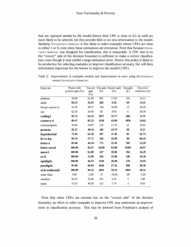
We present a summary of the comparison results in Table 2, where all the measures are the same as in Table 1, except that the baseline comparison is UNCERTAINTY SAM-

PLING rather than RANDOM. BOOTSTRAP-LV exhibits markedly superior performance compared to UNCERTAINTY SAM-

PLING. Particularly, BOOTSTRAP-LV is superior for 13 of the data sets (bold), and for 6 data sets the methods exhibit comparable performance, where phases with positive gain for BOOTSTRAP-LV is between 50% and 60%. UNCERTAINTY SAMPLING exhibits superior performance for one data set, Solar-flare, for which it produces better probability estimations (in the prior comparison for this data set BOOTSTRAP-LV wasn’t considerably better than RANDOM).

Several factors contribute to the weak performance of UNCERTAINTY SAMPLING for CPE compared to BOOTSTRAP-LV. To understand them, recall the differences between UNCERTAINTY SAMPLING and BOOTSTRAP-LV: the effectiveness score each algorithm assigns to potential learning examples and the mechanisms they employ to sample/select examples for labeling. Consider the latter first. Because it uses direct selection, UNCER-

TAINTY SAMPLING does not account for the potential relevance of a learning example for improving the estimation of other examples in the space. It therefore is susceptible to selecting examples with little contribution to the average error across the example space. This may degrade its performance, particularly compared to random sampling. Second, its effectiveness score causes UNCERTAINTY SAMPLING to prefer examples whose CPE is close to 0.5. Thus examples whose true class probability is close to 0.5 and

4 Ensembles usually improve learning curves even with random selection


20

that are captured correctly by the model (hence their CPE is close to 0.5 as well) are more likely to be selected, yet they provide little or no new information to the model. Similarly, UNCERTAINTY SAMPLING is less likely to select examples whose CPEs are close to either 1 or 0, even when these estimations are erroneous. Note that because UNCER-

TAINTY SAMPLING was designed for classification, this is reasonable. A CPE that is on the “correct” side of the decision boundary is sufficient to make a correct classifica-tion, even though it may exhibit a large estimation error. Hence, this policy is likely to be productive for selecting examples to improve classification accuracy, but will deny information important for the learner to improve the model’s CPEs.

Table 2: Improvement in examples needed and improvement in error using BOOTSTRAP-LV

versus UNCERTAINTY SAMPLING

Data set

Phases with positive gain (%)

Top per gain (%)

Top gain (#)

Avg per gain (%)

Avg gain (#)


abalone 50.00 61.09 801 17.63 102 14.11

adult 69.23 35.03 284 9.56 69 11.13 breast cancer-w 55.56 49.37 144 10.90 15 20.20

car 62.50 50.46 68 9.95 6 36.30

coding1 93.75 63.25 1027 31.77 686 6.74 connect-4 89.47 85.52 3230 43.89 1958 54.02 contraceptive 50.00 54.87 126 11.76 21 10.01

german 81.25 48.14 146 24.74 69 8.12 hypothyroid 71.43 62.30 307 17.10 85 62.72 kr-vs-kp 94.74 57.71 144 33.90 90 60.43 letter-a 85.00 44.34 771 15.50 395 21.29 letter-vowel 100.00 81.27 14210 63.80 11463 44.97 move1 100.00 62.89 247 39.96 194 16.29 ocr1 100.00 51.90 256 35.86 146 34.30 optdigits 100.00 44.13 1359 26.08 570 34.91 pendigits 95.00 60.85 1636 27.45 996 38.30 sick-euthyroid 100.00 84.12 1692 59.13 1093 40.51 solar-flare 0.00 -2.98 -17 -16.66 -69 -1.64

weather 56.25 35.06 351 6.32 3 1.98

yeast 53.33 40.38 121 7.74 3 6.03

Note that when CPEs are extreme but on the “correct side” of the decision

boundary, an effort to select examples to improve CPE may undermine an improve-ment in classification accuracy. This may be inferred from Friedman’s analysis of


21

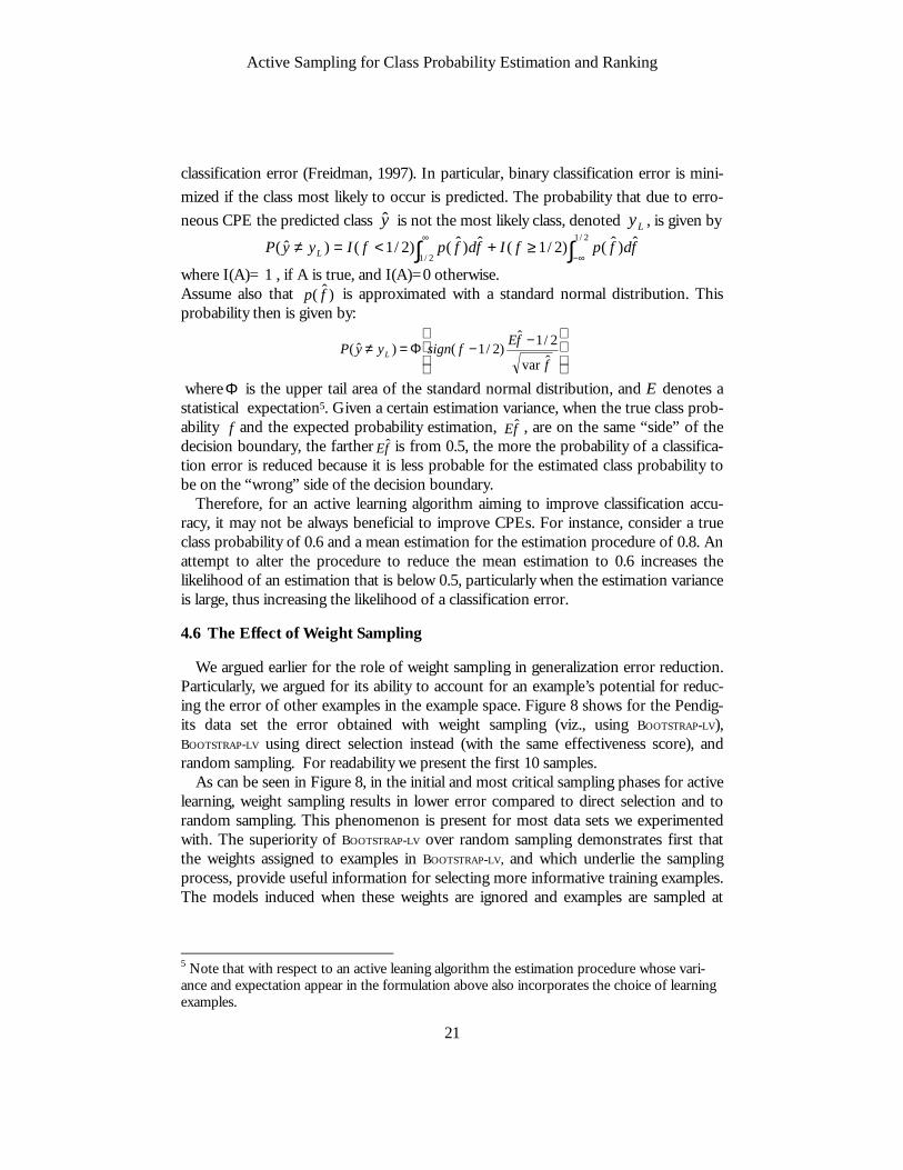
classification error (Freidman, 1997). In particular, binary classification error is mini-mized if the class most likely to occur is predicted. The probability that due to erro-neous CPE the predicted class y is not the most likely class, denoted Ly , is given by

∫∫ ∞−

∞≥+<=≠

2/1

2/1ˆ)ˆ()2/1(ˆ)ˆ()2/1()ˆ( fdfpfIfdfpfIyyP L

where I(A)= 1 , if A is true, and I(A)=0 otherwise. Assume also that )ˆ( fp is approximated with a standard normal distribution. This probability then is given by:

−−Φ=≠f

fEfsignyyP L ˆvar

2/1ˆ)2/1()ˆ(

whereΦ is the upper tail area of the standard normal distribution, and E denotes a statistical expectation5. Given a certain estimation variance, when the true class prob-ability f and the expected probability estimation, fEˆ , are on the same “side” of the decision boundary, the farther fEˆ is from 0.5, the more the probability of a classifica-tion error is reduced because it is less probable for the estimated class probability to be on the “wrong” side of the decision boundary.

Therefore, for an active learning algorithm aiming to improve classification accu-racy, it may not be always beneficial to improve CPEs. For instance, consider a true class probability of 0.6 and a mean estimation for the estimation procedure of 0.8. An attempt to alter the procedure to reduce the mean estimation to 0.6 increases the likelihood of an estimation that is below 0.5, particularly when the estimation variance is large, thus increasing the likelihood of a classification error.

4.6 The Effect of Weight Sampling

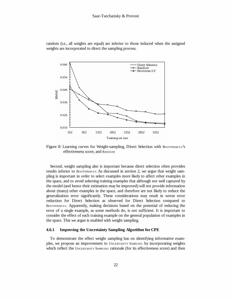
We argued earlier for the role of weight sampling in generalization error reduction. Particularly, we argued for its ability to account for an example’s potential for reduc-ing the error of other examples in the example space. Figure 8 shows for the Pendig-its data set the error obtained with weight sampling (viz., using BOOTSTRAP-LV), BOOTSTRAP-LV using direct selection instead (with the same effectiveness score), and random sampling. For readability we present the first 10 samples.

As can be seen in Figure 8, in the initial and most critical sampling phases for active learning, weight sampling results in lower error compared to direct selection and to random sampling. This phenomenon is present for most data sets we experimented with. The superiority of BOOTSTRAP-LV over random sampling demonstrates first that the weights assigned to examples in BOOTSTRAP-LV, and which underlie the sampling process, provide useful information for selecting more informative training examples. The models induced when these weights are ignored and examples are sampled at

5 Note that with respect to an active leaning algorithm the estimation procedure whose vari-ance and expectation appear in the formulation above also incorporates the choice of learning examples.


22

random (i.e., all weights are equal) are inferior to those induced when the assigned weights are incorporated to direct the sampling process.

Figure 8: Learning curves for Weight-sampling, Direct Selection with BOOTSTRAP-LV’s

effectiveness score, and RANDOM Second, weight sampling also is important because direct selection often provides

results inferior to BOOTSTRAP-LV. As discussed in section 2, we argue that weight sam-pling is important in order to select examples more likely to affect other examples in the space, and to avoid selecting training examples that although not well captured by the model (and hence their estimation may be improved) will not provide information about (many) other examples in the space, and therefore are not likely to reduce the generalization error significantly. These considerations may result in worse error reduction for Direct Selection as observed for Direct Selection compared to BOOTSTRAP-LV. Apparently, making decisions based on the potential of reducing the error of a single example, as some methods do, is not sufficient. It is important to consider the effect of each training example on the general population of examples in the space. This we argue is enabled with weight sampling.

4.6.1 Improving the Uncertainty Sampling Algorithm for CPE

To demonstrate the effect weight sampling has on identifying informative exam-ples, we propose an improvement to UNCERTAINTY SAMPLING by incorporating weights which reflect the UNCERTAINTY SAMPLING rationale (for its effectiveness score) and then

0.016

0.026

0.036

0.046

0.056

0.066

352 852 1352 1852 2352 2852 3352

Training set size

BM

AE

Direct SelectionRandomBootstrap-LV


23

to weight-sample examples according to their weights. We will show how the per-formance of this algorithm improves CPE and compare it to BOOTSTRAP-LV. Since UNCERTAINTY SAMPLING selects examples whose CPE is close to 0.5, we assign to each example a weight that reflects this distance. In particular, at each sampling phase s, the weight assigned to example ix is given by ( )

Rp

xW iis

−−=

5.05.0)( , where

R is a normalization factor such that W is a distribution. The probability of an exam-ple being sampled increases the closer its CPE is to 0.5. The algorithm denoted WEIGHTED UNCERTAINTY SAMPLING (WUS), is described in Figure 9 below. Input: an initial labeled set L, an unlabeled set UL, an inducer I, a stopping criterion, and an integer M specifying the number of actively selected ex-amples in each phase. 1 While stopping criterion not met /* perform next phase: */ 2 Apply inducer I to L

3 For each example { ULxx ii ∈| } assign weight ( )R

pxW i

is

−−=

5.05.0)(

4 Sample from the probability distribution sW , a subset S of M examples from UL without replacement

5 Remove S from UL, label examples in S, and add them to L 6 end for Output: estimator E induced with I from L

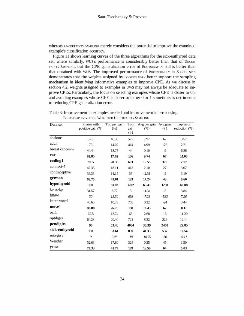
Figure 9: WEIGHTED UNCERTAINTY SAMPLING Algorithm Comparing the new WUS algorithm with BOOTSTRAP-LV for CPE we see that WUS is much more competitive with BOOTSTRAP-LV than UNCERTAINTY SAMPLING. A summary of the results is presented in Table 3. BOOTSTRAP-LV outperforms WUS for 8 data sets (in bold), BOOTSTRAP-LV and WUS are comparable for 10 data sets and WUS is superior in two (italicized). In comparison BOOTSTRAP-LV provides superior CPEs compared to UNCERTAINTY SAMPLING for 14 out of 20 data sets. For six data sets in which UNCERTAINTY

SAMPLING is inferior to BOOTSTRAP-LV, WUS exhibits comparable performance to that of BOOTSTRAP-LV. Overall BOOTSTRAP-LV remains superior, yet the new WEIGHTED UNCER-

TAINTY SAMPLING algorithm exhibits improved performance compared to UNCERTAINTY

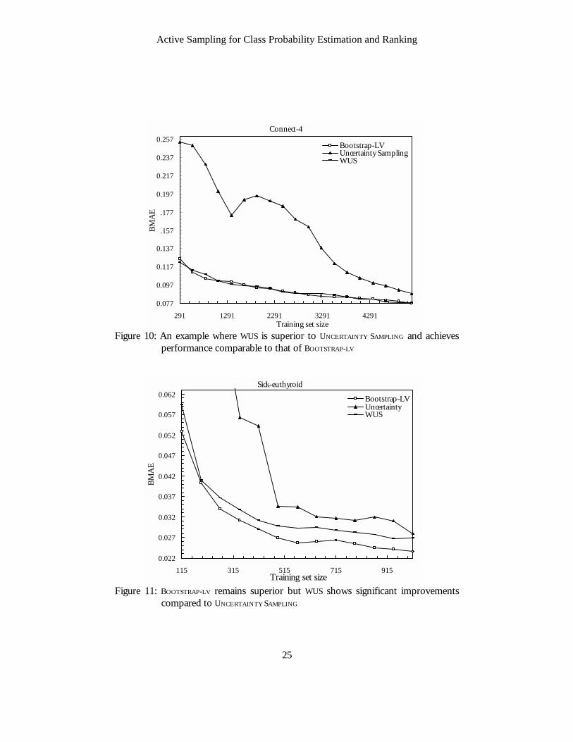
SAMPLING. Figure 10 shows CPE learning curves for the BOOTSTRAP-LV, UNCERTAINTY SAMPLING

and UWS for the Connect-4 data set. Whereas UNCERTAINTY SAMPLING is inferior to BOOTSTRAP-LV for the Connect-4 data set, WUS’s performance is comparable to that of BOOTSTRAP-LV. This can be primarily attributed to WUS accounting for a broader set of considerations when selecting examples, particularly WUS’s consideration of the po-tential error reduction effect an example may have on other examples in the space,


24

whereas UNCERTAINTY SAMPLING merely considers the potential to improve the examined example’s classification accuracy.

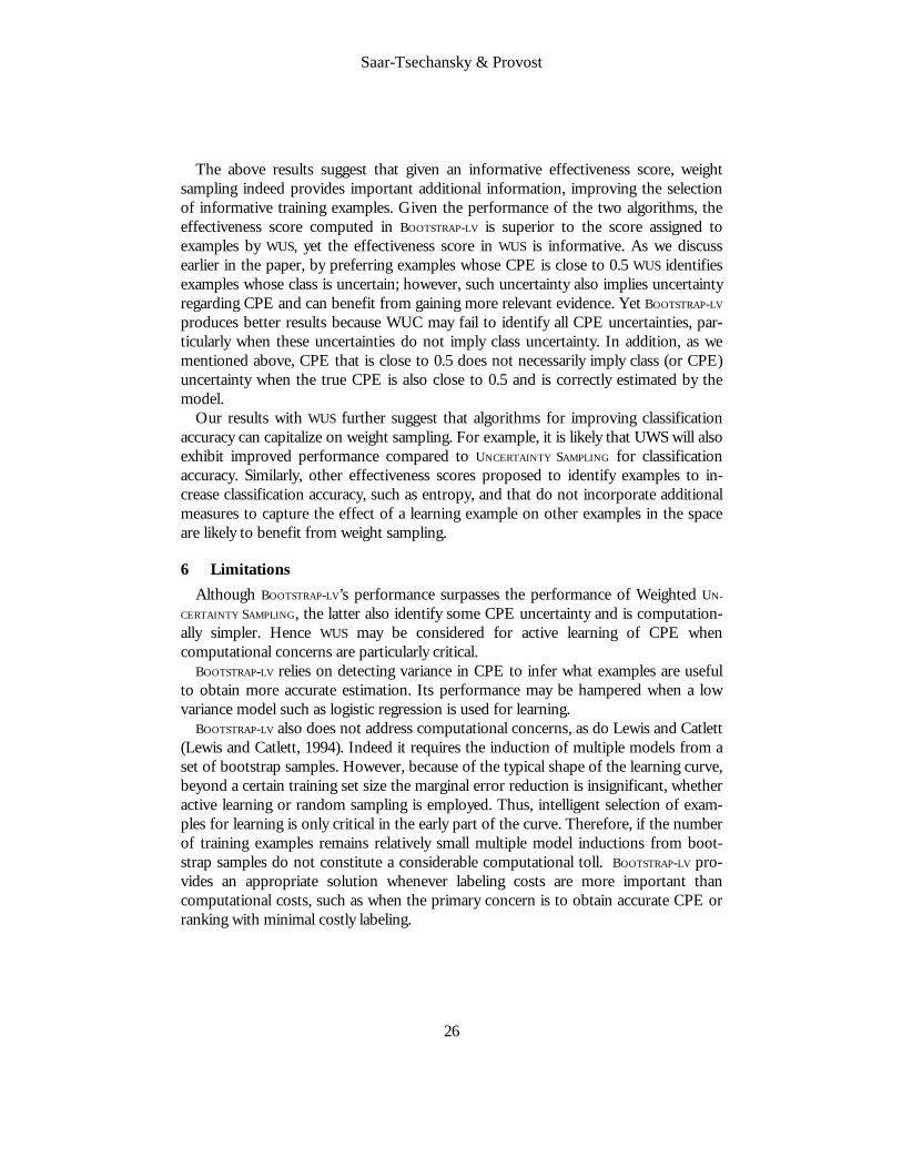
Figure 11 shows learning curves of the three algorithms for the sick-euthyroid data set, where similarly, WUS’s performance is considerably better than that of UNCER-

TAINTY SAMPLING, but the CPE generalization error of BOOTSTRAP-LV still is better than that obtained with WUS. The improved performance of BOOTSTRAP-LV in 8 data sets demonstrates that the weights assigned by BOOTSTRAP-LV better support the sampling mechanism in identifying informative examples to improve CPE. As we discuss in section 4.2, weights assigned to examples in UWS may not always be adequate to im-prove CPEs. Particularly, the focus on selecting examples whose CPE is closer to 0.5 and avoiding examples whose CPE is closer to either 0 or 1 sometimes is detrimental to reducing CPE generalization error. Table 3: Improvement in examples needed and improvement in error using

BOOTSTRAP-LV versus WEIGHTED UNCERTAINTY SAMPLING Data set

Phases with positive gain (%)

Top per gain (%)

Top gain (#)

Avg per gain (%)

Avg gain (#)


abalone 57.1 46.30 577 7.97 62 3.57 adult 76 14.07 414 4.99 123 2.71 breast cancer-w 44.44 18.75 44 0.10 -9 6.86 car 92.85 17.62 136 9.74 67 14.08 coding1 87.5 28.33 671 16.55 379 2.77 connect-4 47.36 18.11 413 2.10 27 3.07 contraceptive 33.33 14.15 58 -2.51 -5 3.19 german 68.75 43.01 133 17.24 43 6.66 hypothyroid 100 81.83 1782 65.41 1260 62.08 kr-vs-kp 31.57 3.77 5 -1.34 -5 3.84 letter-a 30 13.30 693 -7.23 -583 7.26 letter-vowel 46.66 10.73 765 0.32 -24 3.44 move1 88.88 26.73 138 13.45 62 8.11 ocr1 62.5 13.74 66 2.68 16 11.20 optdigits 64.28 20.40 721 8.32 229 12.14 pendigits 90 53.40 4064 36.39 2468 22.85 sick-euthyroid 100 53.61 859 41.33 537 17.54 solar-flare 0 2.46 -19 -16.79 -56 -9.11 Weather 52.63 17.80 328 0.35 45 1.50 yeast 73.33 41.79 189 16.59 64 5.03


25

Figure 10: An example where WUS is superior to UNCERTAINTY SAMPLING and achieves performance comparable to that of BOOTSTRAP-LV

Figure 11: BOOTSTRAP-LV remains superior but WUS shows significant improvements

compared to UNCERTAINTY SAMPLING

Connect-4

0.077

0.097

0.117

0.137

0.157

0.177

0.197

0.217

0.237

0.257


BMA

EBootstrap-LVUncertainty SamplingWUS

Sick-euthyroid

0.022

0.027

0.032

0.037

0.042

0.047

0.052

0.057

0.062


BMA

E

Bootstrap-LVUncertaintyWUS


26

The above results suggest that given an informative effectiveness score, weight sampling indeed provides important additional information, improving the selection of informative training examples. Given the performance of the two algorithms, the effectiveness score computed in BOOTSTRAP-LV is superior to the score assigned to examples by WUS, yet the effectiveness score in WUS is informative. As we discuss earlier in the paper, by preferring examples whose CPE is close to 0.5 WUS identifies examples whose class is uncertain; however, such uncertainty also implies uncertainty regarding CPE and can benefit from gaining more relevant evidence. Yet BOOTSTRAP-LV produces better results because WUC may fail to identify all CPE uncertainties, par-ticularly when these uncertainties do not imply class uncertainty. In addition, as we mentioned above, CPE that is close to 0.5 does not necessarily imply class (or CPE) uncertainty when the true CPE is also close to 0.5 and is correctly estimated by the model.

Our results with WUS further suggest that algorithms for improving classification accuracy can capitalize on weight sampling. For example, it is likely that UWS will also exhibit improved performance compared to UNCERTAINTY SAMPLING for classification accuracy. Similarly, other effectiveness scores proposed to identify examples to in-crease classification accuracy, such as entropy, and that do not incorporate additional measures to capture the effect of a learning example on other examples in the space are likely to benefit from weight sampling.

6 Limitations Although BOOTSTRAP-LV’s performance surpasses the performance of Weighted UN-

CERTAINTY SAMPLING, the latter also identify some CPE uncertainty and is computation-ally simpler. Hence WUS may be considered for active learning of CPE when computational concerns are particularly critical.

BOOTSTRAP-LV relies on detecting variance in CPE to infer what examples are useful to obtain more accurate estimation. Its performance may be hampered when a low variance model such as logistic regression is used for learning.

BOOTSTRAP-LV also does not address computational concerns, as do Lewis and Catlett (Lewis and Catlett, 1994). Indeed it requires the induction of multiple models from a set of bootstrap samples. However, because of the typical shape of the learning curve, beyond a certain training set size the marginal error reduction is insignificant, whether active learning or random sampling is employed. Thus, intelligent selection of exam-ples for learning is only critical in the early part of the curve. Therefore, if the number of training examples remains relatively small multiple model inductions from boot-strap samples do not constitute a considerable computational toll. BOOTSTRAP-LV pro-vides an appropriate solution whenever labeling costs are more important than computational costs, such as when the primary concern is to obtain accurate CPE or ranking with minimal costly labeling.


27

7 Conclusions BOOTSTRAP-LV was designed to use fewer labeled training data to produce accurate

class probability estimates. The algorithm addresses two key components of active learning: an effectiveness score and a selection procedure, which complement each other to identify particularly informative examples for learning class probability esti-mates. BOOTSTRAP-LV is domain independent and is not restricted to a particular learn-ing algorithm.

An empirical evaluation of the approach shows that it performs remarkably well. The evaluation encompasses a wide range of benchmark domains providing compre-hensive evidence for the efficacy of the algorithm. We show how the information provided by the effectiveness scores produces better results than can be obtained with random sampling (i.e., when all weights are equal). We also show that BOOTSTRAP-LV outperforms an existing active learning method, UNCERTAINTY SAMPLING. We investi-gate the properties of the algorithms to explain our empirical results. In particular, the experimental results demonstrate how both the weights assigned to potential training examples and the weight sampling procedure combine to produce superior CPEs. We also examine the properties of the UNCERTAINTY SAMPLING algorithm compared to those of BOOTSTRAP-LV to explain the comparison in performance for estimating class prob-abilities.

Lastly, we use the results of this investigation to propose another active learning al-gorithm, WEIGHTED UNCERTAINTY SAMPLING, which assigns effectiveness scores reflecting the rationale of UNCERTAINTY SAMPLING’s effectiveness score, but which in addition, employs the scores to weight sample examples for training. A comparison with BOOT-

STRAP-LV reveals that BOOTSTRAP-LV still is superior for improving CPEs, demonstrating the value of BOOTSTRAP-LV’s effectiveness score, but also demonstrates the advantages conferred by weight sampling. Our empirical analysis suggests the application of weight sampling with other effectiveness scores proposed in the literature for the active learning of classifiers.

Making decisions in cost sensitive environments often resorts to decision-theoretic approaches for evaluating alternatives, requiring the estimation of probabilities of events or classes to score alternative outcomes. The cost-sensitive nature of such environments can greatly benefit from active learning of class probability estimations and rankings of alternatives. BOOTSTRAP-LV was designed to address this need. The paper provides a comprehensive study of the performance of the BOOTSTRAP-LV algo-rithm with respect to several alternative approaches and highlights the properties responsible for the observed behavior.

Acknowledgments

We thank Vijay Iyengar for helpful comments. We also thank IBM for a Faculty Partnership

Award and the The Penn State eBusiness Research Center and SAP for their support.


28

References

Abe, N. and Mamitsuka, H. (1998). Query Learning Strategies using Boosting and

Bagging. In Proceedings of the Fifteenth International Conference on Machine Learning, pp. 1-

9.

Angluin, D. (1998). Queries and concept learning. Machine Learning, 2:319-342, 1988.

Bauer, E., Kohavi, R. (1999). An Empirical Comparison of Voting Classification Al-

gorithms: Bagging, Boosting, and Variants. Machine Learning, 36, 105-142 (1999).

Blake, C.L. & Merz, C.J. (1998). UCI Repository of machine learning databases. Ir-

vine, CA: University of California, Department of Information and Computer Sci-

ence, 1998 [http://www.ics.uci.edu/~mlearn/MLRepository.html].

Bradley, A. P. (1997). The use of the area under the ROC curve in the evaluation of

machine learning algorithms. Pattern Recognition, 30(7), 1145-1159, 1997.

L. Breiman. (1996). Bagging predictors. Machine Learning, 26(2), 123--140, 1996

Cestnik, B. (1990). Estimating probabilities: A crucial task in machine learning. In

Proceedings of the Ninth European Conference on Artificial Intelligence, 147-149, 1990.

Cohn, D., Atlas, L. and Ladner, R. (1994). Improved generalization with active learn-

ing. Machine Learning, 15:201-221, 1994.

Cohn, D., Ghahramani, Z., and Jordan M. (1996). Active learning with statistical

models. Journal of Artificial Intelligence Research, 4:129-145, 1996.

Cohen, W. W. and Singer, Y. (1999). A simple, fast, and effective rule learner. In pro-

ceedings of the National Conference of the American Association of Artificial Intelli-

gence, 335-342, 1999.

Efron, B. and Tibshirani, R. (1993). An introduction to the Bootstrap, Chapman and Hall,

1997.

Freund, Y. and Shcapire R. (1996). Experiments with a new boosting algorithm. In

Proceedings of the International Conference on Machine Learning, 148-156, 1996.

Iyengar, V. S., Apte, C., and Zhang T. (2000). Active Learning using Adaptive Re-

sampling. In Sixth ACM Special Interest Group on Knowledge Discovery in Databases Inter-

national Conference on Knowledge Discovery and Data Mining. 92-98.


29

Lewis, D. and Gale, W. A. (1994). A sequential algorithm for training text classifiers.

In Association for Computing Machinery-Special Interest Group on Information Retrieval,

1994, 3-12.

Lewis, D. D., and Catlett, J. (1994). Heterogeneous Uncertainty Sampling. In Proceed-

ings of the Eleventh International Conference on Machine Learning, 148-156, 1994.

[Perlich, C.; Provost F.; and Seminoff, J. S. (2001). Tree induction vs. logistic regres-

sion: A learning-curve analysis. CeDER Working Paper #IS-01-02, Stern School of Busi-

ness, NYU.

Provost, F.; Fawcett, T.; and Kohavi, R. (1998). The case against accuracy estimation

for comparing classifiers. In Proceedings of the International Conference on Machine Learn-

ing, 445-453, 1998.

Provost, F. and Domingos P. (2000). Well-trained PETs: Improving Probability Es-

timation Trees. CeDER Working Paper #IS-00-04, Stern School of Business, NYU.

Quinlan, J. R. (1993). C4.5: Programs for machine learning. Morgan Kaufman, San Mateo, California, 1993.

H. S. Seung, M. Opper, and H. Smopolinsky. (1992). Query by committee. In Proceed-

ings of the Fifth Annual ACM Workshop on Computational Learning Theory, 287-294,

1992.

Simon H. A. and Lea G., (1974). Problem solving and rule induction: A unified view.

In L.W. Gregg (ed.), Knowledge and Cognition. Chap. 5. Potomac, MD: Erlbaum, 1974.

Turney, P.D. (2000). Types of cost in inductive concept learning, Workshop on Cost-

Sensitive Learning at ICML-2000, Stanford University, California, 15-21. Valiant L. G. (1984). A theory of the learnable. Communications of the ACM, 27:1134-

1142, 1984.

Winston, P. H. (1975). Learning structural descriptions from examples. In “The Psychol-

ogy of Computer Vision”, P. H. Winston (ed.), McGraw-Hill, New York, 1975.

Zadrozny B. and Elkan C. (2001). Learning and making decisions when costs and

probabilities are both unknown. In the proceedings of The Seventh ACM Special Inter-

est Group on Knowledge Discovery and Data Mining International Conference on Knowledge Dis-

covery and Data Mining. 204-212, 2001.

Active Sampling for Class Probability Estimation and...

Documents

Transcript of Active Sampling for Class Probability Estimation and...