Active Control of Separated Flow over a Circular-Arc AirfoilVortex-shedding frequencies were...

iii

Active Control of Separated Flow over a

Circular-Arc Airfoil

Sergio Miranda

Thesis submitted to the Faculty of the Virginia Polytechnic Institute and State

University in partial fulfillment of the requirements for the degree of

Masters of ScienceIn

Engineering Mechanics

Demetri P. Telionis, ChairDean T. Mook

Muhammad R. HajjScott L. Hendricks

May 8, 2000Blacksburg, Virginia

Keywords: Flow control, wind tunnel testing, airfoil, vortex flow

Copyright 2000, Sergio Miranda

iv

Active Control of Separated Flow over aCircular-arc Airfoil

Sergio Miranda

(ABSTRACT)

An experimental study of active control of fully separated flow over a symmetrical circular-

arc airfoil at high angles of attack was performed. The experiments were carried out in a

low-speed, open circuit wind tunnel. Angles of attack from 10 to 40 degrees were tested.

Low-power input, unsteady excitation was applied to the leading or trailing edge shear

layers. The actuation was provided by the periodic oscillation of a 4-percent-chord flap

placed on the suction side of the airfoil and facing the sharp edge. Vortex-shedding

frequencies were measured and harmonic combinations selected as the applied actuator

frequencies.

Pressure measurements over the airfoil show that the control increased the normal force

coefficient by up to 70%. This supports the idea of vortex capture in the time-averaged

sense, enhancing the lift on the airfoil by managing the shear layer roll up.

The results indicate the viability of the control of large-scale flow fields by exploiting the

natural amplification of disturbances triggered by small-scale actuators.

The application of flow control on sharp-edged aircraft wings could lead to improved

maneuverability, innovative flight control and weight reduction. These can be achieved by

inexpensive, low-power, rugged actuators.

iii

Dedication

To my fiancé Carolina. You did this with me...even from so far away...Te amo~~~!!!

and my parents, who always encouraged and supported me to achieve my dreams.

iv

Acknowledgements

The list is endless if I have to thank all the people that made possible this work.

My first and sincere thanks goes to the mastermind of all I have done: Dr. D. P. Telionis.

He gave me the possibility of studying in the United States and showed me what I

thought nobody could really do: that there are no limits on what we can achieve. We

agreed in many things, disagreed in others, but there was no time where I could not

learn something from him. He supported me from the beginning and never said no to a

new idea. Thanks, from the bottom of my heart.

The other person who I owe an immense gratitude is my laboratory fellow and

friend Matthew Zeiger. He was with me on the worst times of my research, helping with

the pressure acquisition system that he best knows. Thanks for your time and friendship.

I’ll try to catch up on you in golfing...

Working in the ESM Fluids Laboratory allowed me to meet many people,

graduates, undergraduates and technicians. All of them helped me on building this brick

by brick project, and all of them showed me that friendship doesn’t have frontiers. Mark

Carrara, Alexis Telionis, Michael Tadema-Wielandt, Demetri Stamos, Pavlos Vlachos,

Robert Hodges, Sandra Klute, Yasser El-Okda. I will never forget you guys.

Friends outside the Lab helped me to forget my research difficulties and enjoy my

life. All of them participated in this thesis, by relaxing me in the anger times. A special

thanks to my friend and roommate Juan Salcedo, for his friendship and taking me out of

the lab when I most needed it. I can not forget to mention Diego de la Riva, Axel

Castaños, Valerio Viti and all the people I have met in the Latin American and Iberic

Student Association, LAIGSA.

I could never forget to mention Dr. D. T. Mook. I had the pleasure to know him as

a professor and also as a graduate committee advisor. His comments were always more

than helpful. I really enjoyed those afternoons of spanish conversations.

I also want to thank Dr. M. R. Hajj and S. L. Hendricks for integrating my

committee and spending their valuable time for me. I had the pleasure to meet them as a

teaching assistant, and respect them for their simplicity and wisdom.

The Engineering Science and Mechanics department would not be the same

without Loretta Tickle. She was the solution for all the problems, and she solved each of

them efficiently. She puts her heart on everything she does, and I will never forget that.

Thank you.

v

A brief, but more than important thanks goes to Dr. Martinez. You know why...

I don’t want to forget my family, the old one, and the new one (in law’s). All of you

helped me to be here, and e-mails counting can probably show it. Thanks for your love.

At last, but not least, I want to thank the one that made everything possible, from

the very beginning. I owe you this beautiful life, and my love for everything I do. You

know I do my best. Thank you God.

vi

Table of Contents

TABLE OF FIGURES AND MULTIMEDIA OBJECTS VIII

NOMENCLATURE XIII

CHAPTER 1 INTRODUCTION 1

1.1 Flow control 2

1.2 Separated Flow 5

CHAPTER 2 REVIEW OF BASIC CONCEPTS 7

2.1 Physics of Enhancing Vortex Lift by Unsteady Excitation 8

2.1.1 Vortex layer instability-receptivity 9

2.1.2 Resonance 11Sound-Vortex Resonance 12

Vortex-Vortex Resonance 12

2.1.3 Streaming 13Acoustic Streaming 13

Vortical Streaming 14

CHAPTER 3 LITERATURE REVIEW 15

3.1 Relevant Previous Work 15

3.2 Conclusions 32

CHAPTER 4 EXPERIMENTAL SETUP AND EQUIPMENT 34

4.1 Introduction 34

4.2 Wind Tunnel 34

4.3 Airfoil model and instrumentation 36

4.3.1 Airfoil Model 36

4.3.2 Actuation System 40

4.3.3 Feedback Sensor 42

4.3.4 Strain Gage Balance 44

vii

4.3.5 Pitot Rake 49

4.4 Data Acquisition System and Additional Instrumentation 52

CHAPTER 5 EXPERIMENTAL RESULTS 55

5.1 Rake Calibration and Positioning 55

5.2 Data Acquisition Process 58

5.3 Results 64

5.3.1 Base flow 64

5.3.2 Controlled Case 70

5.4 Balance Results 90

CHAPTER 6 CONCLUSIONS AND PROPOSED WORK 94

REFERENCES 96

VITA 99

viii

Table of Figures and Multimedia Objects

Figure 1.1.1 Classification of flow control strategies (from Gad-el-Hak, 1998) 3

Figure 1.1.2 Different control loops for active flow control (from Gad-el-Hak, 1998) 4

Figure 1.2.1 Separated/Separating Flows and possible actuation 5

Figure 2.1 The mean CL ~ α of a flat plate. From Wicks (1954) (Taken From Wu’s

paper) 7

Figure 2.1.1.1 Sketch of initial mixing layer. From Ho and Huerre (1984). (Taken

From Wu’s paper) 9

Figure 2.1.1.2 Variations of normalized amplification rate of the perturbed free vortex

layer. From Ho and Huerre (1984) (Taken From Wu’s paper). Linear stability

theory: R = 1; ⋅ R= 0.5; - - - R << 1. Experiments: 7 , \\\ R = 1 ; x R =

0.72; D R = 0.31. 10

Figure 2.1.1.3 Subharmonic and vortex merging. From Ho (1981)(Taken From Wu’s

paper). 10

Figure 3.1 Vortex-generator test configurations shown approximately to scale. From

Bursnall (1952). 16

Figure 3.2 Sketch of testing model. From Zhou et al (1993). 17

Figure 3.3 Variation of lift coefficient with forcing frequency. °= 27α ,51065.6Re x= . From Zhou et al (1993). 18

Figure 3.4 Distribution of pressure coefficient. °= 27α , 51065.6Re x= . From Zhou

et al (1993). 18

Figure 3.5 Relation between vortex shedding frequency and forcing frequency.

°= 27α , 51071.6Re x= . From Zhou et al (1993). 19

Figure 3.6 Turbulence energy in the wake. y′is the vertical distance in the wind-

tunnel coordinates, with 0=′y at the leading edge of the airfoil. °= 27α ,

51071.6Re x= , 615.1=cx . Open symbols: unforced; closed: forced with

2=f . From Zhou et al (1993). 19

Figure 3.7 Mean velocity profile in the wake. y′is the same as in Figure 3.6,

°= 27α , 51071.6Re x= , 615.1=cx , 15.0=cz . Open symbols: unforced;

closed: forced with 2=f . From Zhou et al (1993). 20

ix

Figure 3.8 a) Schematic of experimental arrangement, b) coordinate system of the

flap motion, and c) oscillating mode shapes of the flap motion. From Hsiao et

al (1998). 22

Figure 3.9 Variation of normalized lift coeffitients over an airfoil with excitation

frequency at different angles of attack for 5100.3Re x= and forcing at a

1.25% chord. Arrow indicates bigger 0ll CC , with the base positioned at

10 =ll CC . From Hsiao et al (1990). 23

Figure 3.10 a) Maximum velocity fluctuation; b) the corresponding sound pressure

level at the slot exit; and c) the lift coefficient at constant driven voltage and

AOA = 22°. From Chang et al (1992). 24

Figure 3.11 a) Maximum velocity fluctuation; b) the corresponding SPL; and c) the lift

coefficient at AOA = 22° and driven by a low-frequency loudspeaker. From

Chang et al (1992). 25

Figure 3.12 Airfoil pressure distributions with and without excitation for angles of

attack : a) 26° and b) 28°. From Hsiao et al (1994). 26

Figure 3.13 Schematic diagram of a synthetic jet. From Crook et al (1999). 27

Figure 3.14 Experimental set-up for active control of stalled flow around an airfoil by

impinging vortex rings. From Kiya et al (1999). 28

Figure 3.15 a) Flow visualization of the separated flow affected by the impinging

vortex rings. Flow is from left to right. The phase-averaged reattachment

position is indicates by the open triangles. Coordinates of position of the

vortex rings are denoted by the solid triangles on the x and vertical y axes; b)

Phase-averaged velocity distributions q~ in the separated flow affected by the

impinging vortex rings. The phase-averaged reattachment position is indicated

by the open triangles. Coordinates of position of the vortex rings are denoted

by the solid triangles on the x and y axed. Thin solid lines indicate the

distributions of the time-averaged velocity q~ in the undisturbed shear layer,

while the solid lines show the center o the shear layer. 30

Figure 3.16 5.0=sa ff , %5.2=µC , with αµ sincUlvCmax ∞= being

cl %5.2= and max

v the maximum perturbation velocity. a) Instantaneous lift

and drag coefficients. b) Power spectral density of Cl. 31

Figure 3.17 As Figure 3.16 but 2=sa ff . 32

x

Figure 4.2.1 ESM Wind Tunnel. From Seider (1984) 35

Figure 4.3.1.1 Airfoil model dimensions (inches) 38

Figure 4.3.1.2 Model geometry and pressure taps location 39

Figure 4.3.1.3 Pressure taps construction 39

Figure 4.3.1.4 32 Channel PSI ESP Pressure Scanner 40

Figure 4.3.2.1 Flap close up view 41

Figure 4.3.2.2 Flap Detail 42

Figure 4.3.2.3 High current adjustable voltage regulator 43

Figure 4.3.3.1 Complete model schematic 44

Figure 4.3.3.2 Complete airfoil model 45

Figure 4.3.3.3 Close up view of the actuating/sensing mechanism 45

Figure 4.3.4.1 Strain Gage Balance 46

Figure 4.3.4.2 Strain gage balance 47

Figure 4.3.4.3 Balance/Wing system and degrees of freedom. 48

Figure 4.3.4.4 Universal joint exploded view. 49

Figure 4.3.5.1 Pitot Rake Positioning 51

Figure 4.3.5.2 Pitot Rake 51

Figure 4.4.1 Schematic diagram of the experimental set up 53

Figure 5.1.1 Circular cylinder positioning for rake calibration 55

Figure 5.1.2 Frequency spectrum on the rake for V∞= 16.2 m/sec 56

Figure 5.1.3 Comparison of results for circular cylinder vortex shedding 57

Figure 5.1.4 Vortex shedding visualization for rake alignment, smU /5.6=∞ ;a) Angle

of attack 50°, b) Angle of attack 30°. 59

Figure 5.2.1 Schematic of flap positions tested. a) Leading edge flap; b) trailing edge

flap. 60

Figure 5.2.2 Pressure taps measured in the experiment. 62

Figure 5.3.1.1 Airfoil pressure coefficient distribution at different angles of attack.

Suction and pressure sides. No actuation. For Reynolds number, see Table

5.2.1. 64

Figure 5.3.1.2 Power spectrum density on the rake for pitots 1 through 3. Angle of

attack 20°. smU /5.17=∞ 66

Figure 5.3.1.3 Power spectrum density on the rake for pitots 4 through 6. Angle of

attack 20°. smU /5.17=∞ 66

xi

Figure 5.3.1.4 PSD at angles 40° through 25°. Pitot 3. Reynolds number and

freestream velocity as in Table 5.2.1. PK: peak values. 67

Figure 5.3.1.5 PSD at angles 20° through 10°. Pitot 3. Reynolds number and

freestream velocity as in Table 5.2.1. PK: peak values. 67

Figure 5.3.1.6 Base flow normal force coefficient with respect to time at different

angles of attack. Freestream velocity and Reynolds number from Table 5.2.1.

Avr: average value. 69

Figure 5.3.2.1 Normal force coefficient variation with excitation frequency. Angle of

attack: 40°; � leading edge flap actuation; ê trailing edge flap actuation. 71

Figure 5.3.2.2 Strouhal number variation with excitation frequency. Angle of attack:

40°; � leading edge flap actuation; ê trailing edge flap actuation. 71






attack: 25°; leading edge flap actuation. 73


25°; leading edge flap actuation. 73






attack: 15°; leading edge flap actuation. 75




attack: 10°;leading edge flap actuation. 76



Figure 5.3.2.13 PSD of pitot 3 at excitation |F|=2.06. Angle of attack 30° 78

Figure 5.3.2.14 PSD of pitot 3 at excitation |F|=1.75. Angle of attack 25°. Pk: peaks. 79

xii

Figure 5.3.2.15 Pressure coefficient distribution for controlled case. Angle of attack

20°. Leading edge excitation. 80

Figure 5.3.2.16 PSD of pitot 3 for controlled case. Angle of attack 20°. Leading edge

excitation. 81

Figure 5.3.2.17 Evolution of normal force coefficient for different actuation

frequencies. Angle of attack 20°. Leading edge excitation. 82


20°. Trailing edge excitation. 83

Figure 5.3.2.19 PSD of pitot 4 for controlled case. Angle of attack 20°. Trailing edge

excitation. 83


frequencies. Angle of attack 20°. Trailing edge excitation. 84




excitation. 86






excitation. 89



Figure 5.4.1 Natural frequency spectrum for the balance system. 91

Figure 5.4.2 Integrated pressure over the suction side of the airfoil. °= 30α ,

smU /10=∞ . 92

Figure 5.4.3 Balance output voltage for the lift channel. °= 30α , smU /10=∞ . 92

Table 5.2.1 Experiment parameters on the airfoil testing. LE: leading edge; TE:

trailing edge 62

Table 5.2.2 Pressure taps location 63

xiii

Nomenclature

θ Flap angleL Liftρ Flow Density

Γ Circulationθ Shear layer thickness

iα Imaginary part of the complex wave number

lC Section lift coefficient

pC Pressure coefficient

nC Section normal force coefficient

U Velocity / Velocity on the shear layerc Airfoil Chordf Frequency

P Pressureα Angle of attack

|F| Reduced frequency sa ff≡|Str| Normalized Strouhal number 0StrStr≡|Cn| Normalized section normal force coefficient 0nn CC≡

Subscripts:

stall Static stall condition∞ Free streama Actuators Sheddingsuc Airfoil suction sidepres Airfoil pressure side

0 Base case, no control applied.

1

Chapter 1 Introduction

Over the past few decades, there has been a marked trend towards the design of

fighter aircraft with low radar signature and at the same time capable of flying at

supersonic regimes, maintaining high levels of maneuverability. This kind of configurations

involve many physical and technical limitations, setting a new challenge to the industry.

Sharp edges are a common feature on these airframes, and separation can not be

avoided for even low angles of attack. The need for complex flap systems or swept wing

configurations with stable lifting vortices is part of the tools that designers use to achieve

high levels of agility and also flight at angles of attack well beyond the maximum lift.

Flow control is a new approach in the design of new radical configurations. The

suction side of the wings for low-observable fighter aircraft is dominated by separated flow

that comprises of large and small vortices with a wide spectrum of length scales and

frequencies. Active control of this vortical structure could serve for different purposes at

different flight regimes and angles of attack. Recent experimental and numerical evidence

shows that at high angles of attack, it is indeed possible to increase lift by as much as 70

percent by controlling the vortex forming process of separated flows. This can be achieved

by utilizing low power actuators, effectively controlling the shear layer roll up over the wing.

The system could provide an effective way of aerodynamic controls reducing or

eliminating the required moving surfaces, or trimming the aircraft without incurring an

increase of drag. This could lead to an important reduction in take off weight and airframe

simplicity. It is also possible to permit the aircraft to fly efficiently at post-stall angles of

attack, improving turn performance in air combat. The structures could benefit by this new

approach as well. Buffeting control may reduce the airloads, leading to a possible

reduction of the structure weight and also having a deep impact on the life on the airframe.

All these could be implemented via fast computers that permit the management of multiple

feedback parameters present in the control of the flow field over these configurations.

The goal of this research is to get a better insight into the flow field over these

configurations, and analyze the effects of the control on the aerodynamic characteristics. A

two-dimensional circular-arc airfoil is chosen as the test bed for the analysis of flow control

at high angles of attack. This is a necessary step for the understanding of the vortex lift

augmentation control on the subsonic regime of supersonic, stealth wing configurations.

Attached flow can not be sustained over a sharp edge leading edge even at low angles of

2

attack. A different means of flow control has to be put in practice: flow control of separated

flows.

Before proceeding further, we provide here a short description of the concepts of

flow control.

1.1 Flow control

Man has never been satisfied with the world that surrounds him, and tried to control

or improve it from the very beginning to get more beneficial effects. This applies to almost

all science disciplines nowadays, and fluid Mechanics is not an exception. Since early

times, fluid was an attractive and at the same time difficult to understand subject that

forced investigators to improve their skills and knowledge. Even after understanding some

of the complicated fluid behavior investigators were never satisfied, and put also their

efforts on controlling it. That’s where the discipline of Flow Control was born.

It is hard to provide a definition for flow control, but one that could closely fit with

this work is given by Fiedler (1998): “...is a process or operation by which certain

characteristics of a given flow are manipulated in such a way as to achieve improvements

or a specific technical performance”.

This definition of flow control is bounded by the fact that this manipulation is

effectuated by “...the internal amplification of a small ‘tailored; disturbances”. The word

‘control’ might seem too strict or even arrogant in the sense that the flow is just induced to

behave in a given form. This control is just a triggering of the natural unsteadiness by

means of a low power actuator. In such a way that the flows develops naturally in the

desired form.

An excellent introduction and historical perspective of flow control can be found in

Gad-el-Hak (1998). From there, we can make use of two figures that show where we stand

in this research in terms of the applied control. Figures 1.1.1 and 1.1.2 show the flow

control strategies and feedback loops for different forms of actuation. Figure 1.1.1 basically

provides the distinction between passive and active actuation and the active different

classifications. The active control differs from the passive in the sense that auxiliary power

is required. The reactive active control is that one where a control signal is taken from

measurements of the flow, whereas in the predetermined case, the control is not

dependent on the flow condition. Reactive flow itself divides in feedforward, where the

measured variable and the controlled variable differ (applying a control law); and feedback,

3

where the controlled variable is measured, fed back, and compared with a reference input.

The feedback reactive control is also subdivided in different control methods.

The possible control loops are depicted in Figure 1.1.2. a) shows a typical

predetermined active control strategy, being an open loop. The reactive active flow control

can be an open feedforward loop as in b) or a closed feedback one as in c). As we will see

later, the control loop used in this work is of the reactive active type, using an open

feedforward control loop.

Figure 1.1.1 Classification of flow control strategies (from Gad-el-Hak, 1998)

FeedbackFeedforward

ReactivePredetermined

ActivePassive

Flow control Strategies

Optimal controlDynamical SystemPhysical modelAdaptive

4

(a)

(b)

(c)

Figure 1.1.2 Different control loops for active flow control (from Gad-el-Hak, 1998)

Controller

(Actuator)

Power

Controlledvariable

Controlledvariable

Measuredvariable

Feedforwardsignal

SensorController

(Actuator)

Power

Measured/controlledvariable

Feedforwardvariable

-

+

Reference

Feedbacksignal

Feedforward element

(Actuator)Comparator

Feedforward element

(Actuator)

5

1.2 Separated Flow

Our goal is to be able to control the separated flow over a thin circular-arc airfoil.

For that matter, we should clarify here the difference between separated flow control and

flow separation control. Both imply the condition of a detached flow, but in a different flow

scale. Fiedler (1998) makes a clear distinction between these two flow fields. This is

shown in Figure 1.2.1.

Figure 1.2.1 Separated/Separating Flows and possible actuation

Weak separation can be defined as that one where the separation point is variable

or undefined. That is the case for most flow fields around airplanes (ex: flow over a wing),

where the separation point depends solely on the surface contour and flight condition.

When separation occurs, the wall boundary layer detaches from the wall and develops into

Passive

Separation Flow Control

Strong separationWeak separation

Separating/separated flows

Active

− Optimal Shape

− Vortex generators

− Vibrating flaps

− Acoustic excitation

− Suction and/or blowing

(steady or periodic)

Separated Flow Control

6

a free shear layer. Since the free shear layer is more susceptible to control than the

boundary layer itself, any attempt of control has to introduce a perturbation directly into it.

The strong separation case is the one where the separation point is fixed. This is

the one that applies to this work, and to mostly all bluff bodies with sharp corners. The

separation point is usually fixed at a sharp edge or corner.

For both the strong and weak separation cases, passive and active controls are possible.

The latter is less effective and more compromising. The shape is optimized to one flight

regime, and can not be changed, unless leading and trailing edge flaps are used1. In the

case of bluff bodies, passive control has a more limited application, influencing the flow in

a reduced way.

Active control, has shown to be more effective and flexible in its application. It is

also not as intrusive as vortex generators, and can produce substantial increases in L/D.

Various practical means of applying active control are shown in Figure 1.2.1. All of these

have been experimentally explored and shown to yield different results.

In the specific case of airfoils aerodynamics, it is important to notice that this classification

depends on the leading edge radius. For sharp leading edges, the airfoil is going to

behave as a bluff body even for the low α range. This is because there is an inmediate

separation due to the large unfavorable pressure gradient existing at the sharp edge. This

separation is normally prevented by the use of leading edge flaps.

For rounded leading-edge airfoils, the weak or strong separation classification

depends strictly on the angle of attack. Wu et al. (1998) make a nice distinction between

these to cases, and this is how Figure 1.2.1 also classifies the conditions. For the angle of

attack range α < αstall, the flow is not fully separated, and the control is aimed at

overcoming separation. Usually the result is the complete elimination of the separated flow

at a given α or the reattachment of the flow downstream, creating a recirculating bubble.

For α > αstall the flow is fully separated, and is most uncertain that the control will promote

reattachment. This defines two control categories: separation control and separated flow

control.

This research falls into the category of active control of a strong separation, ie.

separated flow control. The actuation is applied by means of an oscillating flap either on

the leading or trailing edge.

1 New materials are giving the possibility of modify the wing shape in flight to achieve the optimizedcondition. This are the so-called smart wings, modifying camber and thickness as required.

7

Chapter 2 Review of Basic Concepts

The area of separated flow control is full of empirical relations and physical

interpretations, but a theory that could back up all experiments performed to the date is still

missing. This is due to the complexity of the flow, and its highly non-linear behavior. An

excellent review and starting point for this kind of flow control is given by Wu et al. (1991),

who discuss the maximum lift achieved at super high angles of attack, and the aircraft

maneuvering possibilities that this opens. They show how a simple flat plate has a second

maximum lift peak at a very high angle of attack, as shown in Figure 2.1.

Figure 2.1 The mean CL ~ α of a flat plate. From Wicks (1954) (Taken From Wu’s paper)

The idea is to break through the unsteady separation barrier by enhancing the flow

separation and unsteadiness in a controlled manner using unsteady excitation. This would

lead to the third generation of aeronautical types of flow, with weakly unsteady detached

vortex flow.

The overall idea is to increase lift by capturing a vortex in the suction side of the

wing in the average sense.The Kutta-Joukowsky lift formula relates the lift with the amount

of circulation around the wing by:

8

Γ−= UL ρ

If a vortex is captured in the average sense, an increase in lift will be induced due to the

additional circulation around the airfoil. In order to create an increment in lift, there can not

be counter rotating vortices over the airfoil, since this would destroy any total circulation.

This means that if a strong vortex over the wing can’t be sustained, then vortex shedding

must exist. Should the vortex shedding be completely controlled or eliminated? Not

necessarily: vortex shedding can exist if in the average a non-zero circulation is generated.

Wu et al (1991) discuss different experiments done in the past and how they tried to

achieve the vortex lift by different means. They emphasize the fact that in the 2-D

experiments, the vortex is unstable and has the tendency to become three-dimensional.

The only possible way to stabilize the vortex is by inducing a strong axial velocity in the

spanwise direction. This is how slender wings can maintain a stable vortex on their leading

edges without control, since the vortex generated has a strong core axial velocity. They

don’t need flow control since this is the natural way the vortex appears in this kind of flow,

in its stable state. Anyway, if angle of attack is highly increased on a slender wing, vortex

shedding occurs, detaching the vortices unsteadily from the upper surface. This would

repeat again the behavior observed in the 2-D case for even lower angles of attack. The

difference is that in the 2-D case, a stable vortex can’t exist, and detaches immediately.

But it is important to notice that even when the flow field over a 2-D airfoil and a slender

wing are completely different, there are still analogies between them for high angles of

attack.

Different theoretical models were tried without real application to the vortex capture

phenomenon. This problem is difficult to model, invloving a strong nonlinear interaction

and unsteadiness of thin vortex layers and shed vortices.

2.1 Physics of Enhancing Vortex Lift by Unsteady Excitation

In the same paper, Wu et al (1991) summarize the physics of the vortex lift

enhancement by unsteady excitation. This can be resumed in a chain of events:

vortex layer instability-receptivity-resonance-streaming

9

These are the mechanisms that take place in the flow field and need to be understood in

order to devise an effective method to control the flow and capture a vortex.

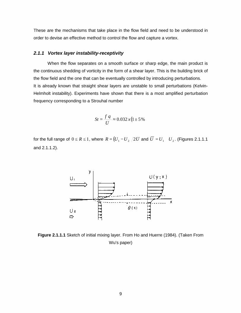
2.1.1 Vortex layer instability-receptivity

When the flow separates on a smooth surface or sharp edge, the main product is

the continuous shedding of vorticity in the form of a shear layer. This is the building brick of

the flow field and the one that can be eventually controlled by introducing perturbations.

It is already known that straight shear layers are unstable to small perturbations (Kelvin-

Helmholt instability). Experiments have shown that there is a most amplified perturbation

frequency corresponding to a Strouhal number

( )%51032.0 ±≈= xUf

Stθ

for the full range of 10 ≤≤R , where ( ) UUUR 221 −= and 21 UUU += . (Figures 2.1.1.1

and 2.1.1.2).

Figure 2.1.1.1 Sketch of initial mixing layer. From Ho and Huerre (1984). (Taken From

Wu’s paper)

10

Figure 2.1.1.2 Variations of normalized amplification rate of the perturbed free vortex

layer. From Ho and Huerre (1984) (Taken From Wu’s paper). Linear stability theory: R

= 1; ⋅ R= 0.5; - - - R << 1. Experiments: 7 , \\\ R = 1 ; x R = 0.72; D R = 0.31.

As the vortex layer evolves, it rolls up into vortices which soon start interacting with

each other. The sub-harmonic instability plays its role, causing the vortex merging at half

the fundamental frequency with double wave length. This is shown in Figure 2.1.1.3.

Figure 2.1.1.3 Subharmonic and vortex merging. From Ho (1981)(Taken From Wu’s

paper).

11

The process goes on repeating this behavior, doubling the vortex size each time and

increasing the layer thickness. This describes the local interaction of the vortices. A global

effect is produced due to the upstream influence of the downstream stronger concentrated

vortices. This is called feedback mechanism and adds its effects to the local instability.

Vortex pairing and the growth of shear layers are strongly affected by small

external excitation. This is the receptivity problem: how certain modes are excited by

imposed disturbances. Depending on the forcing frequency, the response frequency of the

shear layer will set to a particular harmonic. The important fact is that very low forcing

levels ( )U%1.001.0 − are needed if the forcing frequency is properly chosen.

The application of a straight vortex layer is practically of no use in the present case,

since the shear layer will be a rolled-up one. Howoever, the fundamental behavior of the

rolled-up and straight vortex layer is similar, and stability and receptivity fundamentals can

be interpolated from the latter.

2.1.2 Resonance

The concept of resonance here is closely related to the one known from simple

oscillation theory. If the forcing terms on a linear oscillator have the same frequency as

that of the fundamental mode of the linear oscillator, then an internal resonance appears

and leads to an enhanced response. The resonant response of this oscillation, might be

favorable or not, and if the former is encountered, then due to the amplification and

organizing effects of the internal resonance it provides a potential for managing the

unsteady detached flow.

Since the resonance is the result of the interaction of two periodic events

syncronized in phase with frequencies that are integer multiples of each other, we need a

periodic flow feature and feedback mechanism which is in phase with the former in order

to enable the disturbance to interact to itself In this form, with a low power input and using

the natural frequency of the system, the amplitude of the excitations can be greatly

improved. For our application, the resonance of interest is the wave-vortex resonance. The

waves include:

− Sound waves, being longitudinal acoustic/shock waves, generated from normal

perturbations in unsteady processes.

− Vortex waves, being transverse vortical waves, generated from tangential

perturbations in unsteady processes.

12

Both cases are inherently coupled, especially in the proximity to solid surfaces. Then, in

order to control de vortex layer development and create favorable resonance, both

acoustic waves and vortex waves can be imposed as forcing sources. Wu et al. (1991)

provide an extensive review of the physics of both cases. The main important points are

presented below.

Sound-Vortex Resonance

This appears as the resonant interaction of acoustic field and vortical waves in

separated vortex layers. Many experiments were performed, and they all show that in

separated flows with sound resonance, good spanwise vortex shedding correlation is

obtained, and great concentration of vorticity. Even when unsteady vortex flow is the

principal generator of acoustic waves, the inverse is not true. In order to create the

resonant condition, there has to be a mechanism by which the normal pressure

fluctuations transfer to tangential pressure fluctuations creating the feedback mechanism.

This process is found to be realized in the wall trough the adherence condition. The sound-

vortex interaction effects the following benefits:

− Allows to set the frequency of unsteady vortex layer evolution

− Presents a natural means of organizing the vortical flow structure

− Possibility of obtaining the most enhanced vortical flow with the least amount of

energy.

The most interesting part in the mechanism of sound-vortex interaction, is that Kutta

condition imposed on sharp edges enhances the mechanism of energy transfer from

acoustic field to the vortex layer or viceversa. Analytical and experimental results show

that sharp edge leading and trailing edges enhance the sound-vortex resonance. In both

cases, the optimum was found, placing the sound source as close to the edge and with the

acoustic waves emanating to the edge off the airfoil.

The sound-vortex resonance is a very flexible system to apply since it can produce

a wide range of frequencies (20 Hz to 30 kHz) and was found to convert 99% of the

incident acoustic energy to vortical energy at resonant frequencies.

Vortex-Vortex Resonance

A mechanical oscillation, as the one implemented in this experiment, produces a

vortical wave that can generate vortex-vortex resonance. Since there is no need for

transformation from normal waves to tangential waves, the vortex-vortex interaction is

13

more straightforward and leads to better vortex shedding frequency fixing. The drawback

is that the frequency range is more limited (110 Hz for this experiment). The simplest

explanation is that the tangential oscillation to the surface produces vortical waves that

establish the vortex-vortex resonance. There are also acoustic waves generated in the

process.

It is important to notice that research has shown that oscillating sharp edges are

more effective than oscillating bluff bodies (see Wu et al, 1991). This is due to the fact that

from a sharp edge the separation is fixed and also the vorticity besides being more

concentrated, has the same sign (compared to a Karman vortex that alternates vortices

signs). This results in less oscillation amplitude needed to achieve the same effect.

There is no systematical theoretical explanation to the vortex-vortex resonance

mechanism. Anyway, experiments show that using proper forcing frequency (by means of

flaps, synthetic jets, etc) results are better than those produced by acoustic excitation,

even when the resonant condition is not arrived at.

The best of both worlds can probably be achieved by blowing/suction. Both vortex

and acoustic waves are generated in the process, and this probably explains the

effectiveness achieved in the experiments.

2.1.3 Streaming

We were able to see that the internal resonance can excite and enhance the well

organized vortical waves. This doesn’t mean though that the overall effect creates a lift

increment. To achieve this, the alternating change of sign of the shed vortices has to be

managed in order to make the net time-averaged circulation non-zero. The definition of

streaming or drift motion comes from the mean motion of a fluid from the nonlinear wave

interaction. As before, we have two forms of streaming due to each wave-vortex

resonance: acoustic streaming and vortical streaming.

Acoustic Streaming

The acoustic streaming can be best understood as the effect of the nonlinear

Reynolds stress in a periodic flow. The necessary mechanism which dissipates the wave

energy converting it into steady streaming, is the viscosity. That means that it is a

nonlinear result of the sound-vortex interaction.

14

It can be shown that the product of the acoustic streaming is vortical flow, therefore, under

given conditions, the acoustic generation can be seen as a steady vorticity source. There

is no theoretical work that analyzes the effect of acoustic streaming on the evolving vortex

layer, but the experiments and understanding of the physics show that this is effective in

generating organized vortical flows.

Vortical Streaming

Vortical streaming is the vortex flow induced by an incident vortical wave. Like

acoustic streaming, for a vortical streaming to be strong, there must be an effective

mechanism to attenuate the vortical wave and convert its energy to the main vortex. For

incompressible flows, the mechanical dissipation that augments streaming is viscosity.

15

Chapter 3 Literature Review

The area of airfoil research is broad and full of interesting results. Nevertheless,

flow control experiments over separated flow found usually applies only for low speed, low

Mach number conventional airfoils. Experiments performed over supersonic airfoil

configurations, even in the low speed regime, are not available. It’s not strange, since

active flow control is a relatively newcomer to the field.

3.1 Relevant Previous Work

Some declassified literature is available from research done on the early fifties, on

the very beginning of the supersonic flow era. Even in those days, flow control was in the

mind of researchers and engineers, knowing that a sharp leading edge, appropriate for

supersonic flow performed poorly on subsonic regimes. A good indication of that interest is

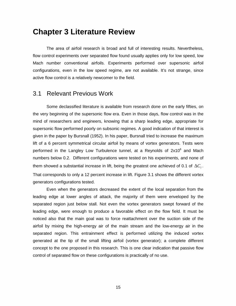
given in the paper by Bursnall (1952). In his paper, Bursnall tried to increase the maximum

lift of a 6 percent symmetrical circular airfoil by means of vortex generators. Tests were

performed in the Langley Low Turbulence tunnel, at a Reynolds of 2x106 and Mach

numbers below 0.2. Different configurations were tested on his experiments, and none of

them showed a substantial increase in lift, being the greatest one achieved of 0.1 of lC∆ .

That corresponds to only a 12 percent increase in lift. Figure 3.1 shows the different vortex

generators configurations tested.

Even when the generators decreased the extent of the local separation from the

leading edge at lower angles of attack, the majority of them were enveloped by the

separated region just below stall. Not even the vortex generators swept forward of the

leading edge, were enough to produce a favorable effect on the flow field. It must be

noticed also that the main goal was to force reattachment over the suction side of the

airfoil by mixing the high-energy air of the main stream and the low-energy air in the

separated region. This entrainment effect is performed utilizing the induced vortex

generated at the tip of the small lifting airfoil (vortex generator); a complete different

concept to the one proposed in this research. This is one clear indication that passive flow

control of separated flow on these configurations is practically of no use.

16

Figure 3.1 Vortex-generator test configurations shown approximately to scale. From

Bursnall (1952).

A completely new approach to control the separated flow over wings with sharp

leading edges was introduced by Zhou et al (1993). Following the theory established in Wu

et al (1991), they tested a NACA 0025 with its sharp leading edge facing upstream, and a

2.2 percent chord flap on the suction side near the leading edge. It must be noted that the

flap oscillation was a mere 0.5-1 mm peak to peak. The tested model can be seen

sketched on Figure 3.2.

17

Figure 3.2 Sketch of testing model. From Zhou et al (1993).

Zhou et al found that at an angle of attack of 27° and with proper frequency, lift was

increased by 60-70% in comparison with the stationary configuration. Both balance

measurements and pressure distributions were acquired on their experiment. Results are

shown in Figures 3.3 and 3.4, where the reduced frequency is given by: ∞⋅= Ucff flap .

Figure 3.3 shows and increment of 70% for 1=f reducing to 60% for 2=f . Zhou et al

make the comment that at lower angles of attack or lower Reynolds numbers, the forcing

effects were smaller, but no results are included. Figure 3.4 shows that when the forcing is

imposed, a separated region containing a strong vortex in the upper surface is attained in

the mean sense. Reattachment follows close to the trailing edge. Pulsed-wire

measurements made possible a deeper insight and confirmed the existence of the vortex

capturing.

Hot wire measurements in the wake taken from the paper are shown in Figures 3.5,

3.6 and 3.7. The first figure implies that forcing practically made no change in vortex

shedding from the airfoil. Figure 3.6 at the same time, shows a reduction in turbulence

intensity in the wake, that is, a reduction of vorticity carried by each vortex shed from the

airfoil. This means that forcing did not capture singular vortices but prevented vorticity from

18

Figure 3.3 Variation of lift coefficient with forcing frequency. °= 27α , 51065.6Re x= .

From Zhou et al (1993).

Figure 3.4 Distribution of pressure coefficient. °= 27α , 51065.6Re x= . From Zhou et al

(1993).

19

Figure 3.5 Relation between vortex shedding frequency and forcing frequency. °= 27α ,51071.6Re x= . From Zhou et al (1993).

Figure 3.6 Turbulence energy in the wake. y′is the vertical distance in the wind-tunnel

coordinates, with 0=′y at the leading edge of the airfoil. °= 27α , 51071.6Re x= ,

615.1=cx . Open symbols: unforced; closed: forced with 2=f . From Zhou et al (1993).

20

Figure 3.7 Mean velocity profile in the wake. y′is the same as in Figure 3.6, °= 27α ,

51071.6Re x= , 615.1=cx , 15.0=cz . Open symbols: unforced; closed: forced with

2=f . From Zhou et al (1993).

being swept out. The conservation of this vorticity contributed to a time-average large

scale vortex on the upper surface, that incremented lift. The last figure depicts a reduction

of the mean velocity defect. That translates to the fact that there is drag reduction present

as well.

The overall idea gained on this paper is that a huge increase in L/D can be

obtained with a small perturbation applied on the shear layer. The average capturing of a

vortex on the suction side leads to more than beneficial results.

Another interesting paper on flow control over stalled airfoils applying an oscillating

flap actuation is given by Hsiao et al (1993). They instrument a NACA 633-018 airfoil with a

flap mechanism close to the leading edge and study parametrically the effects of position,

amplitude and frequency of the flap motion, as well as the Reynolds number at post-stall

angles of attack. The angles of attack tested are 28°, 31° and 35°, whereas the Reynolds

numbers are 5109.1Re x= and 5102.3Re x= . From the excitation frequency effects,

they can deduce that the most effective forcing frequency is that of the natural shedding

frequency of the vortical structures in the shear layer. Excitation of the first harmonic, sf2 ,

or the first sub-harmonic, 2sf does have some effect, but significantly smaller than the

fundamental forcing.

21

Hsiao et al can see the same effect of excitation on the flow pattern over the airfoil

as Zhou et al : shear layer vortices develop into large vortical structures. These structures

induce high velocity to lower the pressure on the airfoil upper surface. The long time

average of lift can be incremented as much as 50%. Energy spectra of the velocity

fluctuations in the wake region, show that when the natural shedding frequency is forced,

the fundamental mode attains significantly higher energy while it becomes narrower. This

means that the vortical flow pattern becomes more organized due to the effective forcing.

Studies on location and amplitude of the oscillating flap show that both have effects

on lift and drag. Moreover, the aerodynamic properties become more sensitive as

α increases. They believe that at a high angle of attack the development of the rolled-up

vortex is less restricted by the airfoil upper surface. However, efficient control is achieved

when the flap protrudes into the shear region to stimulate the unstable shear layer. At

angles above 40° their flap extended beyond the shear layer, setting the limit for the

actuation system. Amplitude effects proved to be secondary as long as the tip of the flap

protrudes the shear layer.

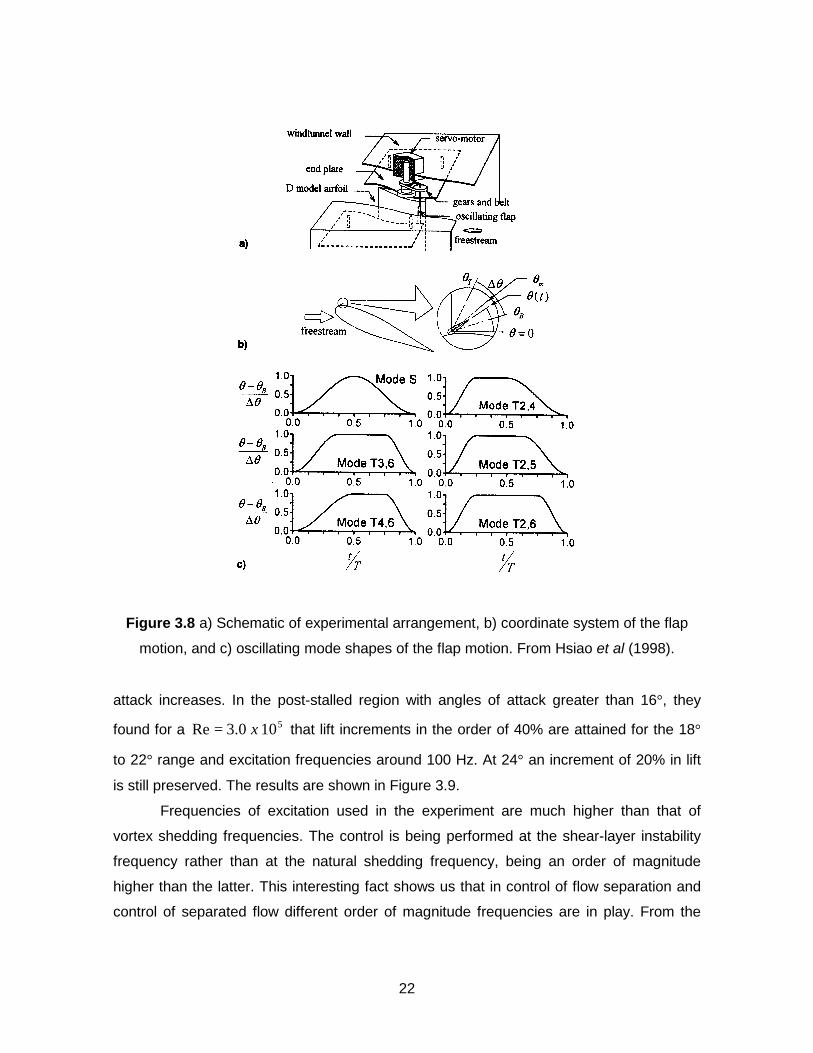
Using the same set up, Hsiao et al (1998) studied the effects of the oscillation

modes shapes on the aerodynamic properties. Different modes of actuation were tested

and are shown in Figure 3.8 along with the experimental arrangement.

The oscillating mode of the flap motion shows to be an important parameter on the

final aerodynamic performance. Excitation mode 6,2T , 6,3T , or 6,4T gives a much better lift

coefficient increase than mode S or 4,2T , whereas mode 5,2T falls in between them. At the

stalled α the most effective mode, 6,2T , obtains a 20-45% extra increase of lift coefficient

in comparison to mode S . Mode 6,2T not only produces a stronger leading-edge vortex,

but also causes an earlier vortex formation and a lower vortex convection speed on the

vortex-enhancement process.

Hsiao et al (1990) applied acoustic excitation of wall-separated flow on the

NACA 633-018. One-mm-wide slots are located at 1.25%, 6.25% and 13.75% chord to

emit acoustic waves coming from a loudspeaker and measure the most effective position.

Even when their goal is to delay stall, controlling separation and favoring reattachment,

their conclusions and comments are valuable. They perform excitation at different

frequency levels in three regions: pre-stalled region, stalled region, and post-stalled region.

Lift increase is negligible for the pre-stalled region, but becomes significant as angle of

22

Figure 3.8 a) Schematic of experimental arrangement, b) coordinate system of the flap

motion, and c) oscillating mode shapes of the flap motion. From Hsiao et al (1998).

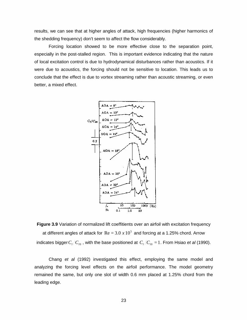
attack increases. In the post-stalled region with angles of attack greater than 16°, they

found for a 5100.3Re x= that lift increments in the order of 40% are attained for the 18°

to 22° range and excitation frequencies around 100 Hz. At 24° an increment of 20% in lift

is still preserved. The results are shown in Figure 3.9.

Frequencies of excitation used in the experiment are much higher than that of

vortex shedding frequencies. The control is being performed at the shear-layer instability

frequency rather than at the natural shedding frequency, being an order of magnitude

higher than the latter. This interesting fact shows us that in control of flow separation and

control of separated flow different order of magnitude frequencies are in play. From the

23

results, we can see that at higher angles of attack, high frequencies (higher harmonics of

the shedding frequency) don’t seem to affect the flow considerably.

Forcing location showed to be more effective close to the separation point,

especially in the post-stalled region. This is important evidence indicating that the nature

of local excitation control is due to hydrodynamical disturbances rather than acoustics. If it

were due to acoustics, the forcing should not be sensitive to location. This leads us to

conclude that the effect is due to vortex streaming rather than acoustic streaming, or even

better, a mixed effect.

Figure 3.9 Variation of normalized lift coeffitients over an airfoil with excitation frequency

at different angles of attack for 5100.3Re x= and forcing at a 1.25% chord. Arrow

indicates bigger 0ll CC , with the base positioned at 10 =ll CC . From Hsiao et al (1990).

Chang et al (1992) investigated this effect, employing the same model and

analyzing the forcing level effects on the airfoil performance. The model geometry

remained the same, but only one slot of width 0.6 mm placed at 1.25% chord from the

leading edge.

24

Hot-wire velocity measurements were performed at the slot exit at different

excitation frequencies. Sound pressure level (SPL) was also measured at the slot exit, and

the results showed that the corresponding maximum theoretical acoustic velocity

fluctuations were only a small percentage to the measured velocity fluctuations u′. They

deduced that this unsteady pulsing of the fluid around the slot is the main disturbance

source affecting the flow field around the airfoil, and not the acoustic waves as it was

believed.

Figure 3.10 and 3.11 shows relevant results for the non calibrated actuation ( maxu′

is not constant through the frequency forcing spectrum) for two different loudspeakers. It is

important to notice that a SPL value of 136 dB is equivalent to maximum acoustic velocity

fluctuations of 0.29 m/sec.

Figure 3.10 a) Maximum velocity fluctuation; b) the corresponding sound pressure level at

the slot exit; and c) the lift coefficient at constant driven voltage and AOA = 22°. From

Chang et al (1992).

25

Again, the results obtained support the fact that the actuation is more effective

when the forcing frequency is “locked-in” to the shear layer instability frequency. This was

examined further by Hsiao et al (1994), by placing the same model at higher angles of

attack, to the high post-stall angles (> 24°). He noted that for the low post-stalled region

(20° - 24°) there is an absence of well-defined peaks in the airfoil wake frequency

spectrum, showing that no significant vortex structure has formed behind the airfoil. At

higher angles, narrow banded peaks are present due to the vortex shedding formation. In

Figure 3.11 a) Maximum velocity fluctuation; b) the corresponding SPL; and c) the lift

coefficient at AOA = 22° and driven by a low-frequency loudspeaker. From Chang et al

(1992).

this regime, they found that the most effective frequency for improving aerodynamic

performance is correlated to the vortex shedding instability frequency in the wake. Under

26

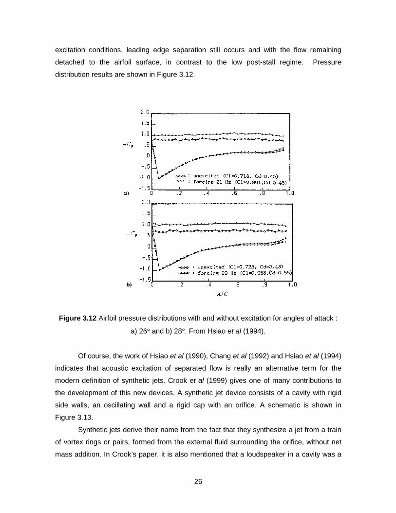
excitation conditions, leading edge separation still occurs and with the flow remaining

detached to the airfoil surface, in contrast to the low post-stall regime. Pressure

distribution results are shown in Figure 3.12.

Figure 3.12 Airfoil pressure distributions with and without excitation for angles of attack :

a) 26° and b) 28°. From Hsiao et al (1994).

Of course, the work of Hsiao et al (1990), Chang et al (1992) and Hsiao et al (1994)

indicates that acoustic excitation of separated flow is really an alternative term for the

modern definition of synthetic jets. Crook et al (1999) gives one of many contributions to

the development of this new devices. A synthetic jet device consists of a cavity with rigid

side walls, an oscillating wall and a rigid cap with an orifice. A schematic is shown in

Figure 3.13.

Synthetic jets derive their name from the fact that they synthesize a jet from a train

of vortex rings or pairs, formed from the external fluid surrounding the orifice, without net

mass addition. In Crook’s paper, it is also mentioned that a loudspeaker in a cavity was a

27

usual form of creating synthetic jets. It is important to note that the sharp edges on the

orifice may contribute through acoustic streaming to the formation of the jet without net

mass flow.

Crook et al (1999) performed some preliminary control of the separation of the

turbulent boundary layer on a circular cylinder, with a single jet positioned just upstream

(93.5 degrees) of the separation point. The device was driven at the natural shedding

frequency, and fluid flow visualization was used to check the effectiveness. The synthetic

jet creates a very strong entrainment of the surrounding fluid, and also penetrates the

boundary layer. They observed a delay in the separation line, even when only one device

is used.

Figure 3.13 Schematic diagram of a synthetic jet. From Crook et al (1999).

A more graphical visualization of the entrainment produced by a synthetic jet is

given in Kiya et al (1999). They performed flow control over a stalled flat plate at an angle

of attack of 10° by introducing vortex rings into the separated layer. The rings were

produced through an orifice of 5 mm bored through the top wind tunnel wall, which was

connected to a woofer through a chamber. Figure 3.14 clarifies the set-up.

Results show that the vortices in the shear layer interact with the vortex ring

yielding a local increase of moment thickness, thus increasing the entrainment rate. A

compact rolling up vortex is created that eliminates the reverse flow on its downstream

side, by transporting high momentum fluid of the main flow towards the surface. This

28

generates a dynamic reattachment moving from 4.0=cx to 8.0=cx , reducing the

separation zone.

Figure 3.14 Experimental set-up for active control of stalled flow around an airfoil by

impinging vortex rings. From Kiya et al (1999).

For this low Reynolds number case (8300), the most effective frequency happens

to be approximately half of the Kelvin-Helmholtz instability. But at higher Reynolds

numbers, the primary mechanism to determine the optimum frequency is the shedding-

type instability. Figure 3.15 presents a sequence of a vortex impinging the plate shear

layer.

Computational Fluid Dynamics (CFD) makes important contributions to the

knowledge of fluid behavior. A paper reflecting the importance of numerical simulations to

post-stall flow control is given by Wu et al (1998). In this paper, the authors perform

Reynolds-averaged two dimensional computations of turbulent flow over an NACA 0012

airfoil at post-stall angles of attack, including periodic blowing-suction excitation located at

the 2.5% of the chord.

The authors show that massively separated and disordered unsteady flow can be

effectively controlled by a local unsteady excitation, with low-level power input. The

unforced random separated flow under proper excitation frequency, becomes periodic or

quasi-periodic. This is associated with a strong lift enhancement. They also show that in

some situations reduction of drag and pressure fluctuations (i.e.: buffeting) is possible.

29

a) b)

Figure 3.15 For caption, see below. Taken from Kiya et al (1999)

30

Figure 3.15 a) Flow visualization of the separated flow affected by the impinging vortex

rings. Flow is from left to right. The phase-averaged reattachment position is indicates by

the open triangles. Coordinates of position of the vortex rings are denoted by the solid

triangles on the x and vertical y axes; b) Phase-averaged velocity distributions q~ in the

separated flow affected by the impinging vortex rings. The phase-averaged reattachment

position is indicated by the open triangles. Coordinates of position of the vortex rings are

denoted by the solid triangles on the x and y axed. Thin solid lines indicate the

distributions of the time-averaged velocity q~ in the undisturbed shear layer, while the solid

lines show the center o the shear layer.

It’s interesting to notice that they focus their attention on the control of the leading

edge shear layer, for its upstream location, highly flexible receptivity, and being the only

source of vortex lift.

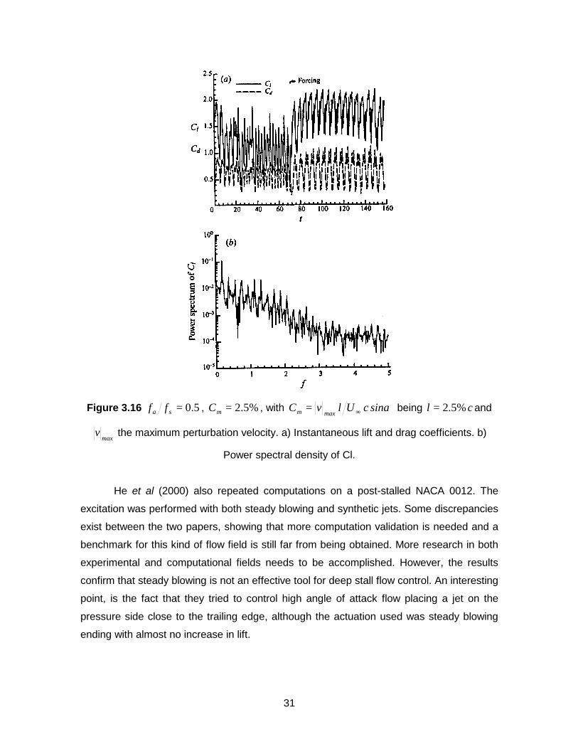
The most effective actuation frequencies were the natural shedding frequency, and

its subharmonics and superharmonics , for angles of attack from 18° to 35°. Lift

enhancement up to 70% was achieved, and random high frequency modes were shown to

be almost suppressed in some cases ( sff 2= ), implying a perfect frequency lock-in. This

is reflected in Figures 3.16 and 3.17.

Wu et al (1998) also explored the physical mechanisms in terms of nonlinear mode

competition and resonance, as well as vortex dynamics, ending with significant

conclusions. They point out that forcing with proper frequency and amplitude can cause

the response frequencies of both shed vortices and shear layer to lock into the harmonics

of the forcing frequency, suppressing other modes. This leads to a well organized flow that

from the vortex-dynamics point of view corresponds to a sufficiently strong entrainment

due to the rolling-in structure of the lifting vortex. To create this vortex, two conditions must

be met. First, the discrete vortices in the shear layer must be forced into rolling-up

coalescence, possible only if the forcing frequency is an order of magnitude lower than the

natural shear-layer frequency, and the forcing amplitude is above a minimum. Second, the

concentrated lifting vortex must be not too far form the airfoil surface, To ensure this

conditions, the angle of attack cannot be too close to stall neither too large.

31

Figure 3.16 5.0=sa ff , %5.2=µC , with αµ sincUlvCmax ∞= being cl %5.2= and

maxv the maximum perturbation velocity. a) Instantaneous lift and drag coefficients. b)

Power spectral density of Cl.

He et al (2000) also repeated computations on a post-stalled NACA 0012. The

excitation was performed with both steady blowing and synthetic jets. Some discrepancies

exist between the two papers, showing that more computation validation is needed and a

benchmark for this kind of flow field is still far from being obtained. More research in both

experimental and computational fields needs to be accomplished. However, the results

confirm that steady blowing is not an effective tool for deep stall flow control. An interesting

point, is the fact that they tried to control high angle of attack flow placing a jet on the

pressure side close to the trailing edge, although the actuation used was steady blowing

ending with almost no increase in lift.

32

Another important difference to Wu et al (1998) is their conclusion that even when

forcing frequency may improve the averaged lift, it also increases the pressure oscillation

amplitudes.

Figure 3.17 As Figure 3.16 but 2=sa ff .

3.2 Conclusions

It is not difficult to conclude that in order to capture a vortex in the average sense

over the airfoil suction side, an efficient way to periodically perturb the leading edge shear

layer is needed. For that reason, the actuation system selected for the current research is

the same as the one utilized by Zhou et al (1993) in their experiment. Even more, the idea

of the flap working as a synthetic jet seems reasonable. If properly sealed and actuating

33

from the fully closed position to a certain angle, flow suction and blowing should occur by

while the flap is moving. This comes from a simple analysis supported by the principle of

conservation of mass in the cavity generated between the flap and airfoil. Neither of the

papers dealing with flaps as the mean of actuation fully investigated the effect of the flap in

the shear layer.

All the papers but one (He et al, 2000) focus their control to the leading edge shear

layer. The actuation of the trailing edge shear layer may also affect the flow through its

global instability. This is one of the points to be studied in the present experiment.

Active Control of Separated Flow over a Circular-Arc AirfoilVortex-shedding frequencies were...

Documents

Transcript of Active Control of Separated Flow over a Circular-Arc AirfoilVortex-shedding frequencies were...