Active Control of Combustion Instability: Theory andPractice

Anuradha M. Annaswamy and Ahmed F. GhoniemDepartment of Mechanical Engineering

MITCambridge, MA

Introduction

One of the most successful applications of control technology in fluid systems is in the context

of dynamic instability in continuous combustion systems. Recent results in this area have shown

unequivocally that active control is not only a feasible technology for reducing the unsteady pres-

sure oscillations, but also that the approach can be scaled up to large-scale industrial rigs. Models

of combustion instability have been derived using both physically based and system-identification

based methods. Optimal, time-delay, and adaptive controllers have been designed using these

models and demonstrated to lead to an order of magnitude improvement in a range of combustion

rigs over empirically designed control methods. In this paper, we present a survey of the existing

theory that includes modeling and control of pressure instability in combustion systems and the

practical applications of active control to-date in small, medium, and large-scale combustion rigs.

Dynamic instability has long been recognized as a problem in continuous combustion systems.

In several applications, including ramjets, rocket motors, afterburners, and gas turbines, this insta-

bility assumes the form of pressure oscillations that have a tendency to grow. Besides the obvious

implications of the increased levels of pressure on the structural integrity of the system compo-

nents, the combined presence of other performance metrics, such as maximizing thermal outputs

and thrust or minimizing emissions, makes a study of this instability and its control extremely

important. In the context of gas turbines, burning at lean operating conditions is attractive from

the standpoint of reduced NOx formation, whereas in propulsion devices such as ramjet engines,

burning under near stoichiometric conditions is desirable since this leads to enhanced heat release

and therefore high performance. Interestingly enough, both of these conditions lead to potentially

unstable behavior.

The recent twist in this old problem is active control. Simple demonstrations on a Rijke tube

1

- Heat Release -

�Acoustics�

6�����

+

Figure 1. Thermoacoustic instability in a combustion system.

in the 1980s showed that by using a very small fraction of the system energy, the pressure ampli-

tude can be reduced by several orders of magnitude, thereby establishing the feasibility of active

combustion control. Subsequently, several laboratory-scale tests were conducted by simulating

conditions of afterburners, ramjets, and gas turbine dynamics and attempting active control of the

ensuing instability. During 1999-2000, several successes were reported in large-scale industrial

rigs, showing that active combustion control is indeed a feasible and viable technology.

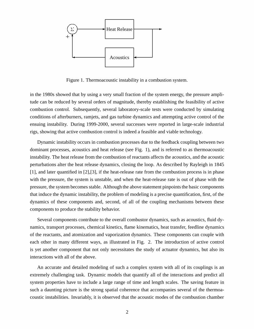
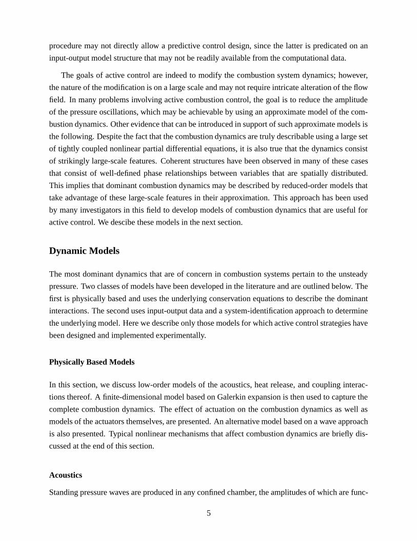
Dynamic instability occurs in combustion processes due to the feedback coupling between two

dominant processes, acoustics and heat release (see Fig. 1), and is referred to as thermoacoustic

instability. The heat release from the combustion of reactants affects the acoustics, and the acoustic

perturbations alter the heat release dynamics, closing the loop. As described by Rayleigh in 1845

[1], and later quantified in [2],[3], if the heat-release rate from the combustion process is in phase

with the pressure, the system is unstable, and when the heat-release rate is out of phase with the

pressure, the system becomes stable. Although the above statement pinpoints the basic components

that induce the dynamic instability, the problem of modeling is a precise quantification, first, of the

dynamics of these components and, second, of all of the coupling mechanisms between these

components to produce the stability behavior.

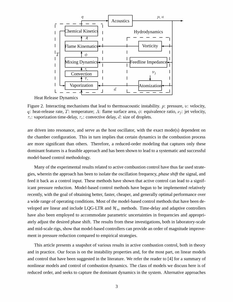
Several components contribute to the overall combustor dynamics, such as acoustics, fluid dy-

namics, transport processes, chemical kinetics, flame kinematics, heat transfer, feedline dynamics

of the reactants, and atomization and vaporization dynamics. These components can couple with

each other in many different ways, as illustrated in Fig. 2. The introduction of active control

is yet another component that not only necessitates the study of actuator dynamics, but also its

interactions with all of the above.

An accurate and detailed modeling of such a complex system with all of its couplings is an

extremely challenging task. Dynamic models that quantify all of the interactions and predict all

system properties have to include a large range of time and length scales. The saving feature in

such a daunting picture is the strong spatial coherence that accompanies several of the thermoa-

coustic instabilities. Invariably, it is observed that the acoustic modes of the combustion chamber

2

-q p; u

Acoustics -

d6

�Vorticity�Flame Kinematics

A6

Chemical Kinetics

�Feedline Impedance�Mixing Dynamics

�6

�c6

�?

�j

Atomization�Vaporization

6�vConvection

-

T

Heat Release Dynamics

Hydrodynamics

Figure 2. Interacting mechanisms that lead to thermoacoustic instability. p: pressure, u: velocity,q: heat-release rate, T : temperature; A: flame surface area, �: equivalence ratio, �j: jet velocity,�v: vaporization time-delay, �v: convective delay, d: size of droplets.

are driven into resonance, and serve as the host oscillator, with the exact mode(s) dependent on

the chamber configuration. This in turn implies that certain dynamics in the combustion process

are more significant than others. Therefore, a reduced-order modeling that captures only these

dominant features is a feasible approach and has been shown to lead to a systematic and successful

model-based control methodology.

Many of the experimental results related to active combustion control have thus far used strate-

gies, wherein the approach has been to isolate the oscillation frequency, phase shift the signal, and

feed it back as a control input. These methods have shown that active control can lead to a signif-

icant pressure reduction. Model-based control methods have begun to be implemented relatively

recently, with the goal of obtaining better, faster, cheaper, and generally optimal performance over

a wide range of operating conditions. Most of the model-based control methods that have been de-

veloped are linear and include LQG-LTR and H1 methods. Time-delay and adaptive controllers

have also been employed to accommodate parametric uncertainties in frequencies and appropri-

ately adjust the desired phase shift. The results from these investigations, both in laboratory-scale

and mid-scale rigs, show that model-based controllers can provide an order of magnitude improve-

ment in pressure reduction compared to empirical strategies.

This article presents a snapshot of various results in active combustion control, both in theory

and in practice. Our focus is on the instability properties and, for the most part, on linear models

and control that have been suggested in the literature. We refer the reader to [4] for a summary of

nonlinear models and control of combustion dynamics. The class of models we discuss here is of

reduced order, and seeks to capture the dominant dynamics in the system. Alternative approaches

3

of using numerical models that involve unsteady calculations of all variables in the flow field using

techniques such as DNS (direct numerical simulation) and LES (large eddy simulation) are not

addressed here but can be found, for example, in [5] and the references therein. More emphasis

is given to models and control methods that have been experimentally validated in some form or

another compared to others that have been verified through numerical simulations.

First, we discuss the highlights of dynamic models and model-based control strategies that

have been developed in the context of combustion instability. Following that, we present results

accruing from experimental investigations in the context of a whole range of rigs ranging from

table top combustors to large-scale industrial rigs. In each case, we describe the configuration of

the rig, the flow conditions, the actuator-sensor used, the control strategies, and the results obtained.

Finally, we outline the status of the current research in active combustion control.

Active Combustion Control: Theory

Two dominant mechanisms that contribute to combustion dynamics are heat-release dynamics and

acoustics. Both of these subprocesses are affected by each other, resulting in a tightly closed feed-

back loop. Several mechanisms provide the coupling interactions between these two processes.

These include agencies that provide velocity perturbations, such as flow impedance, and those that

lead to equivalence ratio perturbations, such as the feedline dynamics. Mechanisms such as vor-

ticity and entropy have also been observed to provide the coupling. These results indicate that a

complete and accurate description of the combustion dynamics consists of several partial differ-

ential equations that describe the acoustics, heat-release dynamics, feedline dynamics, chemical

kinetics, hydrodynamics, transport, and entropy. These equations can then be analyzed using com-

putational procedures that result in the solutions of the flow variables p(x; t), u(x; t), and �(x; t), as

well as the variables that pertain to the heat-release rate q(x; t). Such procedures typically involve

at least a few million state variables and employ methods such as finite difference, finite element,

and vortex element methods. In addition to the large size of the computations involved, additional

complexities arise due to the underlying nonlinearities, whose subtleties make the computing sig-

nificantly harder.

Yet another question that arises is how these computational models can be used to carry out

active control, the goal of which is to modify these dynamics in one form or another. This implies

that the computational procedures need to be carried out not once but several times, each with a

different control action that would result in a different boundary condition, to determine the best

active control input. Also, these solutions may vary significantly from one operating condition

to another, which in turn might require more trial-and-error computing. In addition, the above

4

procedure may not directly allow a predictive control design, since the latter is predicated on an

input-output model structure that may not be readily available from the computational data.

The goals of active control are indeed to modify the combustion system dynamics; however,

the nature of the modification is on a large scale and may not require intricate alteration of the flow

field. In many problems involving active combustion control, the goal is to reduce the amplitude

of the pressure oscillations, which may be achievable by using an approximate model of the com-

bustion dynamics. Other evidence that can be introduced in support of such approximate models is

the following. Despite the fact that the combustion dynamics are truly describable using a large set

of tightly coupled nonlinear partial differential equations, it is also true that the dynamics consist

of strikingly large-scale features. Coherent structures have been observed in many of these cases

that consist of well-defined phase relationships between variables that are spatially distributed.

This implies that dominant combustion dynamics may be described by reduced-order models that

take advantage of these large-scale features in their approximation. This approach has been used

by many investigators in this field to develop models of combustion dynamics that are useful for

active control. We descibe these models in the next section.

Dynamic Models

The most dominant dynamics that are of concern in combustion systems pertain to the unsteady

pressure. Two classes of models have been developed in the literature and are outlined below. The

first is physically based and uses the underlying conservation equations to describe the dominant

interactions. The second uses input-output data and a system-identification approach to determine

the underlying model. Here we describe only those models for which active control strategies have

been designed and implemented experimentally.

Physically Based Models

In this section, we discuss low-order models of the acoustics, heat release, and coupling interac-

tions thereof. A finite-dimensional model based on Galerkin expansion is then used to capture the

complete combustion dynamics. The effect of actuation on the combustion dynamics as well as

models of the actuators themselves, are presented. An alternative model based on a wave approach

is also presented. Typical nonlinear mechanisms that affect combustion dynamics are briefly dis-

cussed at the end of this section.

Acoustics

Standing pressure waves are produced in any confined chamber, the amplitudes of which are func-

5

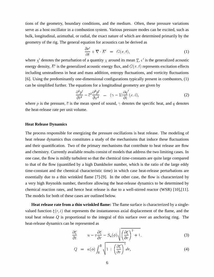
tions of the geometry, boundary conditions, and the medium. Often, these pressure variations

serve as a host oscillator in a combustion system. Various pressure modes can be excited, such as

bulk, longitudinal, azimuthal, or radial, the exact nature of which are determined primarily by the

geometry of the rig. The general equation for acoustics can be derived as

@e0

@t+r �E 0 = G(x; t); (1)

where �0 denotes the perturbation of a quantity � around its mean �, e0 is the generalized acoustic

energy density, E 0 is the generalized acoustic energy flux, and G(x; t) represents excitation effects

including unsteadiness in heat and mass addition, entropy fluctuations, and vorticity fluctuations

[6]. Using the predominantly one-dimensional configurations typically present in combustors, (1)

can be simplified further. The equations for a longitudinal geometry are given by

@2p0

@t2� c2

@2p0

@x2= ( � 1)

@q

@t

0

(x; t); (2)

where p is the pressure, c is the mean speed of sound, denotes the specific heat, and q denotes

the heat-release rate per unit volume.

Heat Release Dynamics

The process responsible for energizing the pressure oscillations is heat release. The modeling of

heat release dynamics thus constitutes a study of the mechanisms that induce these fluctuations

and their quantification. Two of the primary mechanisms that contribute to heat release are flow

and chemistry. Currently available results consist of models that address the two limiting cases. In

one case, the flow is mildly turbulent so that the chemical time-constants are quite large compared

to that of the flow (quantified by a high Damkholer number, which is the ratio of the large eddy

time-constant and the chemical characteristic time) in which case heat-release perturbations are

essentially due to a thin wrinkled flame [7]-[9]. In the other case, the flow is characterized by

a very high Reynolds number, therefore allowing the heat-release dynamics to be determined by

chemical reaction rates, and hence heat release is due to a well-stirred reactor (WSR) [10],[11].

The models for both of these cases are outlined below.

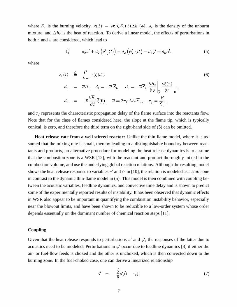
Heat release rate from a thin wrinkled flame: The flame surface is characterized by a single-

valued function �(r; t) that represents the instantaneous axial displacement of the flame, and the

total heat release Q is proportional to the integral of this surface over an anchoring ring. The

heat-release dynamics can be represented as

@�

@t= u� v

@�

@r� Su(�)

vuut @�@r

!2

+ 1; (3)

Q = �(�)Z R

0

vuut1 +

@�

@r

!2

dr; (4)

6

where Su is the burning velocity, �(�) = 2��uSu(�)�hr(�), �u is the density of the unburnt

mixture, and �hr is the heat of reaction. To derive a linear model, the effects of perturbations in

both u and � are considered, which lead to

:Q0

= d0u0 + d1

�u0�f (t)

�+ d2

��0�f (t)

�+ d3�

0 + d� _�0; (5)

where

x� (t)4=

Z t

t��x(�)d�; (6)

d0 = �R; d1 = �� Su; d2 = ��Su

@Su@�

������

@�(r)

@r

�����0

;

d3 = ��@Su

@��(0); � = 2���hrSu; �f =

R

Su

;

and �f represents the characteristic propagation delay of the flame surface into the reactants flow.

Note that for the class of flames considered here, the slope at the flame tip, which is typically

conical, is zero, and therefore the third term on the right-hand side of (5) can be omitted.

Heat release rate from a well-stirred reactor: Unlike the thin-flame model, where it is as-

sumed that the mixing rate is small, thereby leading to a distinguishable boundary between reac-

tants and products, an alternative procedure for modeling the heat release dynamics is to assume

that the combustion zone is a WSR [12], with the reactant and product thoroughly mixed in the

combustion volume, and use the underlying global reaction relations. Although the resulting model

shows the heat-release response to variables u0 and �0 in [10], the relation is modeled as a static one

in contrast to the dynamic thin-flame model in (5). This model is then combined with coupling be-

tween the acoustic variables, feedline dynamics, and convective time delay and is shown to predict

some of the experimentally reported results of instability. It has been observed that dynamic effects

in WSR also appear to be important in quantifying the combustion instability behavior, especially

near the blowout limits, and have been shown to be reducible to a low-order system whose order

depends essentially on the dominant number of chemical reaction steps [11].

Coupling

Given that the heat release responds to perturbations u0 and �0, the responses of the latter due to

acoustics need to be modeled. Perturbations in �0 occur due to feedline dynamics [8] if either the

air- or fuel-flow feeds is choked and the other is unchoked, which is then convected down to the

burning zone. In the fuel-choked case, one can derive a linearized relationship

�0 = ��

uu0s(t� �c); (7)

7

where u0s denotes the velocity perturbation at the exit of the fuel nozzle and �c = L=u, and L is the

distance from the supply to the burning plane. The coupling between u 0 and p0 can be determined

using either the energy or momentum balance relations

@p0

@t+ p

@u0

@x= ( � 1)q0 (8)

@u0

@t+

1

�

@pi@x

= 0: (9)

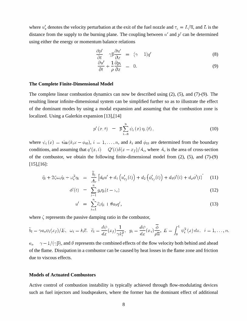
The Complete Finite-Dimensional Model

The complete linear combustion dynamics can now be described using (2), (5), and (7)-(9). The

resulting linear infinite-dimensional system can be simplified further so as to illustrate the effect

of the dominant modes by using a modal expansion and assuming that the combustion zone is

localized. Using a Galerkin expansion [13],[14]

p0 (x; t) = pnXi=0

i (x) �i (t) ; (10)

where i (x) = sin (kix+ �i0), i = 1; : : : ; n, and ki and �i0 are determined from the boundary

conditions, and assuming that q 0(x; t) = Q0(t)Æ(x� xf )=Ac, where Ac is the area of cross-section

of the combustor, we obtain the following finite-dimensional model from (2), (5), and (7)-(9)

[15],[16]:

��i + 2�!i _�i + !2

i �i =ebiAc

hd0u

0 + d1�u0�f (t)

�+ d2

��0�f (t)

�+ d3�

0(t) + d� _�0(t)

i(11)

�0(t) =nXi=1

gi�i(t� �c) (12)

u0 =nXi=1

eci _�i + �a0q0; (13)

where � represents the passive damping ratio in the combustor,

ebi = ao i(xf )=E; !i = kic; eci = d

dx(xf)

1

k2i; gi =

d

dx(xs)

�

�u; E =

Z L

0

2

i (x) dx; i = 1; : : : ; n;

ao = �1=( p), and � represents the combined effects of the flow velocity both behind and ahead

of the flame. Dissipation in a combustor can be caused by heat losses in the flame zone and friction

due to viscous effects.

Models of Actuated Combustors

Active control of combustion instability is typically achieved through flow-modulating devices

such as fuel injectors and loudspeakers, where the former has the dominant effect of additional

8

mass flow, which results in additional heat release, and the latter introduces additional velocity,

which impacts on both acoustics and heat release. Below we present both the models of actuated

combustors and the models of the actuators.

The impact of an acoustic actuator whose diaphragm velocity is vc is given by [17]:

��i + 2�0!�i + !2

i �i = bi:q0

f +bci _vc (14)

y =nXi=1

cci�i; (15)

:q0f =

nXi=1

(gfci:�i +kao�rvc) ; (16)

where y = p0(xs; t)=p, the normalized unsteady pressure component; is the output; xa, xs, and xfare the locations of the actuator, the sensor, and the flame, respectively; kao = 0 if xa > xf and

unity otherwise; bci = �r

E i (xa); cci = i (xs); gf = k�Su�hr; �hr is the heat release rate

per unit mass of the mixture; and k is determined by the flame stabilization mechanism. In (16),

no equivalence ratio perturbations are assumed to be present, and �f is negligible.

If the quantity added is fuel, in addition to the mass flow, heat input is introduced as well, since

it changes the equivalence ratio. Defining

�c =_m0

c

_ma�0;

where _ma is the mean air mass flow rate and �0 is the fuel-to-air ratio at stoichiometry, it can be

shown that when only �0-perturbations are present, the heat release dynamics in (5) is altered as

:Q0

= d2

��0�f (t) + �0c�f

(t� �co)�+ d3(�

0 + �c(t� �co)) + d�( _�0 + _�c(t� �co));

where �co = Lc=u and Lc is the distance between the burning plane and the location of the fuel

injector. If the heat release dynamics are only due to �0-perturbations, for a single-mode model,

the overall combustion model is of the form

�� + 2�! _� + !2� � ��(t� �c) = kc _�c(t� �co): (17)

Actuator Dynamics

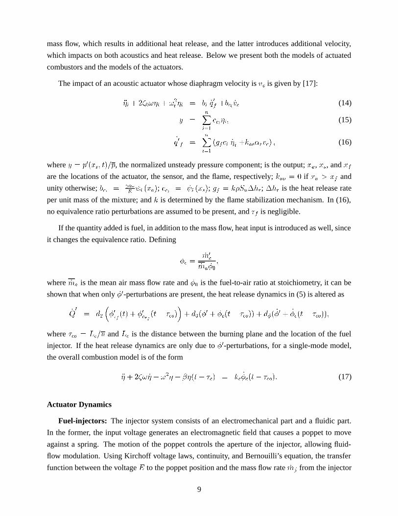
Fuel-injectors: The injector system consists of an electromechanical part and a fluidic part.

In the former, the input voltage generates an electromagnetic field that causes a poppet to move

against a spring. The motion of the poppet controls the aperture of the injector, allowing fluid-

flow modulation. Using Kirchoff voltage laws, continuity, and Bernouilli’s equation, the transfer

function between the voltage E to the poppet position and the mass flow rate _mj from the injector

9

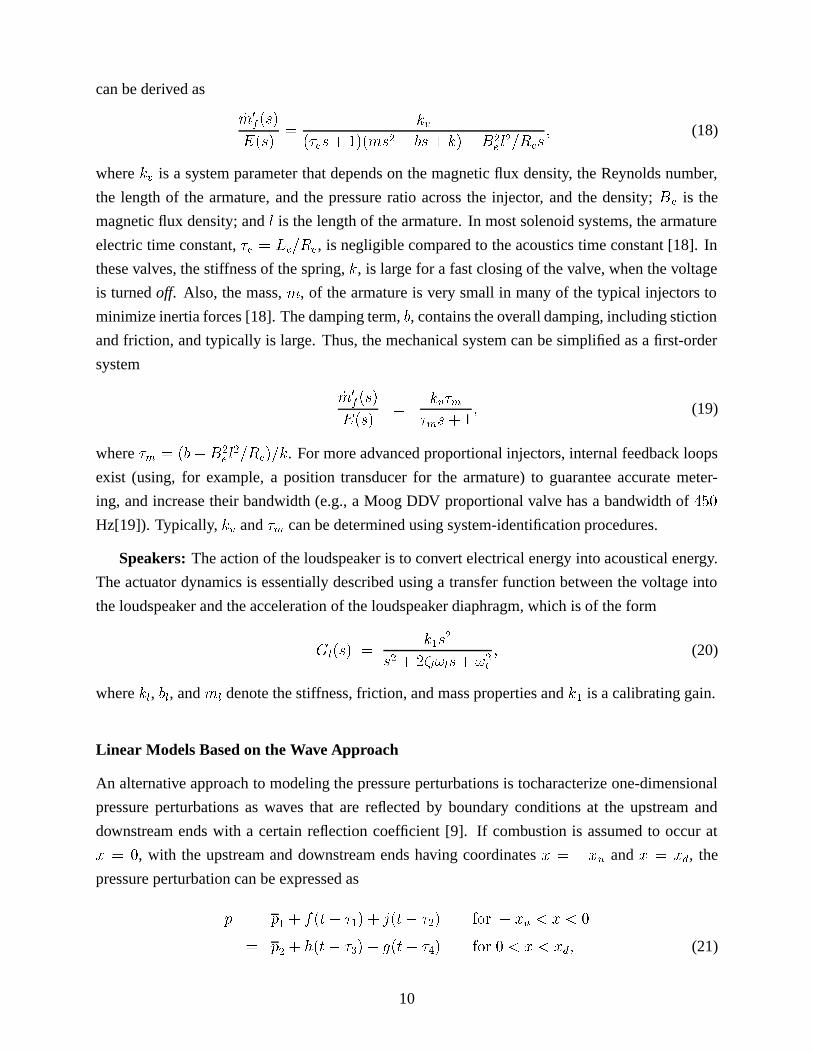
can be derived as

_m0f(s)

E(s)=

kv(�es+ 1)(ms2 + bs + k) +B2

e l2=Res

; (18)

where kv is a system parameter that depends on the magnetic flux density, the Reynolds number,

the length of the armature, and the pressure ratio across the injector, and the density; Be is the

magnetic flux density; and l is the length of the armature. In most solenoid systems, the armature

electric time constant, �e = Le=Re, is negligible compared to the acoustics time constant [18]. In

these valves, the stiffness of the spring, k, is large for a fast closing of the valve, when the voltage

is turned off. Also, the mass, m, of the armature is very small in many of the typical injectors to

minimize inertia forces [18]. The damping term, b, contains the overall damping, including stiction

and friction, and typically is large. Thus, the mechanical system can be simplified as a first-order

system

_m0

f (s)

E(s)=

kv�m�ms+ 1

; (19)

where �m = (b + B2

e l2=Re)=k. For more advanced proportional injectors, internal feedback loops

exist (using, for example, a position transducer for the armature) to guarantee accurate meter-

ing, and increase their bandwidth (e.g., a Moog DDV proportional valve has a bandwidth of 450

Hz[19]). Typically, kv and �m can be determined using system-identification procedures.

Speakers: The action of the loudspeaker is to convert electrical energy into acoustical energy.

The actuator dynamics is essentially described using a transfer function between the voltage into

the loudspeaker and the acceleration of the loudspeaker diaphragm, which is of the form

Gl(s) =k1s

2

s2 + 2�l!ls+ !2

l

; (20)

where kl, bl, and ml denote the stiffness, friction, and mass properties and k1 is a calibrating gain.

Linear Models Based on the Wave Approach

An alternative approach to modeling the pressure perturbations is tocharacterize one-dimensional

pressure perturbations as waves that are reflected by boundary conditions at the upstream and

downstream ends with a certain reflection coefficient [9]. If combustion is assumed to occur at

x = 0, with the upstream and downstream ends having coordinates x = �xu and x = xd, the

pressure perturbation can be expressed as

p = p1 + f(t� �1) + j(t� �2) for � xu < x < 0

= p2+ h(t� �3) + g(t� �4) for 0 < x < xd; (21)

10

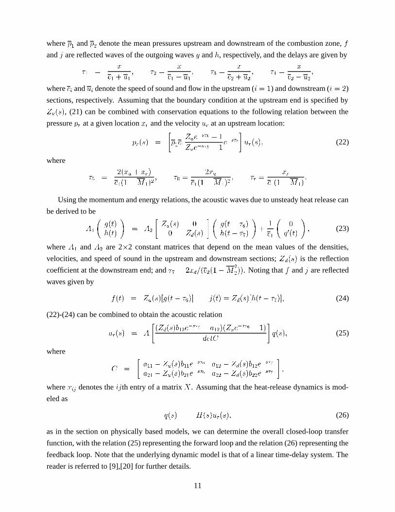
where p1

and p2

denote the mean pressures upstream and downstream of the combustion zone, f

and j are reflected waves of the outgoing waves g and h, respectively, and the delays are given by

�1 =x

c1 + u1; �2 =

x

c1 � u1; �3 =

x

c2 + u2; �4 =

x

c2 � u2;

where ci and ui denote the speed of sound and flow in the upstream (i = 1) and downstream (i = 2)

sections, respectively. Assuming that the boundary condition at the upstream end is specified by

Zu(s), (21) can be combined with conservation equations to the following relation between the

pressure pr at a given location xr and the velocity ur at an upstream location:

pr(s) =

"�1c1

Zue�s�5 + 1

Zue�s�6 � 1e�s�r

#ur(s); (22)

where

�5 =2(xu + xr)

c1(1�M1)2; �6 =

2xuc1(1�M 1)2

; �r =xr

c1(1�M 1):

Using the momentum and energy relations, the acoustic waves due to unsteady heat release can

be derived to be

A1

g(t)h(t)

!= A2

"Zu(s) 00 Zd(s)

# g(t� �6)h(t� �7)

!+

1

c1

0

q0(t)

!; (23)

where A1 and A2 are 2�2 constant matrices that depend on the mean values of the densities,

velocities, and speed of sound in the upstream and downstream sections; Zd(s) is the reflection

coefficient at the downstream end; and �7 = 2xd=(c2(1�M2

2)). Noting that f and j are reflected

waves given by

f(t) = Zu(s)[g(t� �6)] j(t) = Zd(s)[h(t� �7)]; (24)

(22)-(24) can be combined to obtain the acoustic relation

ur(s) = A

"(Zd(s)b12e

�s�7 � a12)(Zue�s�6 � 1)

detC

#q(s); (25)

where

C =

"a11 � Zu(s)b11e

�s�6 a12 � Zd(s)b12e�s�7

a21 � Zu(s)b21e�s�6 a22 � Zd(s)b22e

�s�7

#;

where xij denotes the ijth entry of a matrix X . Assuming that the heat-release dynamics is mod-

eled as

q(s) = H(s)ur(s); (26)

as in the section on physically based models, we can determine the overall closed-loop transfer

function, with the relation (25) representing the forward loop and the relation (26) representing the

feedback loop. Note that the underlying dynamic model is that of a linear time-delay system. The

reader is referred to [9],[20] for further details.

11

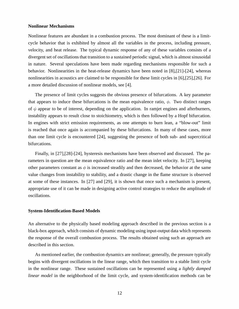
Nonlinear Mechanisms

Nonlinear features are abundant in a combustion process. The most dominant of these is a limit-

cycle behavior that is exhibited by almost all the variables in the process, including pressure,

velocity, and heat release. The typical dynamic response of any of these variables consists of a

divergent set of oscillations that transition to a sustained periodic signal, which is almost sinusoidal

in nature. Several speculations have been made regarding mechanisms responsible for such a

behavior. Nonlinearities in the heat-release dynamics have been noted in [8],[21]-[24], whereas

nonlinearities in acoustics are claimed to be responsible for these limit cycles in [6],[25],[26]. For

a more detailed discussion of nonlinear models, see [4].

The presence of limit cycles suggests the obvious presence of bifurcations. A key parameter

that appears to induce these bifurcations is the mean equivalence ratio, �. Two distinct ranges

of � appear to be of interest, depending on the application. In ramjet engines and afterburners,

instability appears to result close to stoichiometry, which is then followed by a Hopf bifurcation.

In engines with strict emission requirements, as one attempts to burn lean, a “blow-out” limit

is reached that once again is accompanied by these bifurcations. In many of these cases, more

than one limit cycle is encountered [24], suggesting the presence of both sub- and supercritical

bifurcations.

Finally, in [27],[28]-[24], hysteresis mechanisms have been observed and discussed. The pa-

rameters in question are the mean equivalence ratio and the mean inlet velocity. In [27], keeping

other parameters constant as � is increased steadily and then decreased, the behavior at the same

value changes from instability to stability, and a drastic change in the flame structure is observed

at some of these instances. In [27] and [29], it is shown that once such a mechanism is present,

appropriate use of it can be made in designing active control strategies to reduce the amplitude of

oscillations.

System-Identification-Based Models

An alternative to the physically based modeling approach described in the previous section is a

black-box approach, which consists of dynamic modeling using input-output data which represents

the response of the overall combustion process. The results obtained using such an approach are

described in this section.

As mentioned earlier, the combustion dynamics are nonlinear; generally, the pressure typically

begins with divergent oscillations in the linear range, which then transition to a stable limit cycle

in the nonlinear range. These sustained oscillations can be represented using a lightly damped

linear model in the neighborhood of the limit cycle, and system-identification methods can be

12

used for determing the model parameters. As is well known, the system identification procedure

requires (i) input and output data selection, (ii) model structure selection, (iii) determination of the

‘best’ model in the structure as guided by the data, and (iv) selection of an appropriate persistently

exciting input [30]. A control strategy based on such a model will then reduce the output of the

linear model and thus the amplitude of the limit cycle. Such an approach has been used for swirl-

stabilized rigs [31],[32] and for tube-combustors [33], and the results of the former are presented

in the section on active combustion control practice. In [31], two different models, including the

ARMAX and the N4SID methods [30],[34], have been used, whose distinctions lie mainly in how

the impact of external noise on the system dynamics is modeled. For example, in the ARMAX

approach, the model is given by

Ay = Bu+ Ce; (27)

where u and y are the input and the output; e represents exogenous noise, which includes the effect

of nonlinearity; and A;B;C are the system parameters. Prediction error methods and subspace

methods are used in the ARMAX and N4SID models, respectively, for parameter estimation using

a persistently exciting reference signal such as a band-limited white noise. Typically, in most

combustion systems, the input is a voltage to the fuel injector and the output is the pressure sensed

in the combustor. The reader is referred to [31] for further details.

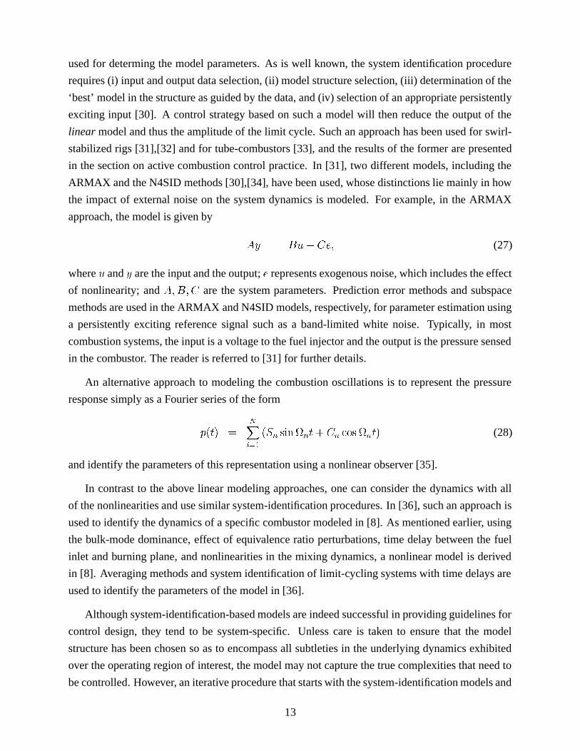
An alternative approach to modeling the combustion oscillations is to represent the pressure

response simply as a Fourier series of the form

p(t) =NXi=1

(Sn sinnt+ Cn cos nt) (28)

and identify the parameters of this representation using a nonlinear observer [35].

In contrast to the above linear modeling approaches, one can consider the dynamics with all

of the nonlinearities and use similar system-identification procedures. In [36], such an approach is

used to identify the dynamics of a specific combustor modeled in [8]. As mentioned earlier, using

the bulk-mode dominance, effect of equivalence ratio perturbations, time delay between the fuel

inlet and burning plane, and nonlinearities in the mixing dynamics, a nonlinear model is derived

in [8]. Averaging methods and system identification of limit-cycling systems with time delays are

used to identify the parameters of the model in [36].

Although system-identification-based models are indeed successful in providing guidelines for

control design, they tend to be system-specific. Unless care is taken to ensure that the model

structure has been chosen so as to encompass all subtleties in the underlying dynamics exhibited

over the operating region of interest, the model may not capture the true complexities that need to

be controlled. However, an iterative procedure that starts with the system-identification models and

13

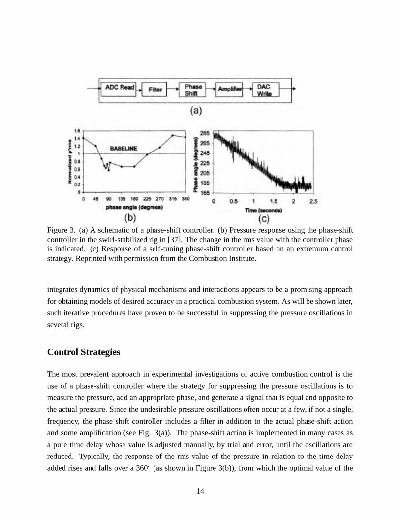
Figure 3. (a) A schematic of a phase-shift controller. (b) Pressure response using the phase-shiftcontroller in the swirl-stabilized rig in [37]. The change in the rms value with the controller phaseis indicated. (c) Response of a self-tuning phase-shift controller based on an extremum controlstrategy. Reprinted with permission from the Combustion Institute.

integrates dynamics of physical mechanisms and interactions appears to be a promising approach

for obtaining models of desired accuracy in a practical combustion system. As will be shown later,

such iterative procedures have proven to be successful in suppressing the pressure oscillations in

several rigs.

Control Strategies

The most prevalent approach in experimental investigations of active combustion control is the

use of a phase-shift controller where the strategy for suppressing the pressure oscillations is to

measure the pressure, add an appropriate phase, and generate a signal that is equal and opposite to

the actual pressure. Since the undesirable pressure oscillations often occur at a few, if not a single,

frequency, the phase shift controller includes a filter in addition to the actual phase-shift action

and some amplification (see Fig. 3(a)). The phase-shift action is implemented in many cases as

a pure time delay whose value is adjusted manually, by trial and error, until the oscillations are

reduced. Typically, the response of the rms value of the pressure in relation to the time delay

added rises and falls over a 360Æ (as shown in Figure 3(b)), from which the optimal value of the

14

delay (or the corresponding phase) is determined. In [37], an adaptive version of the phase-shift

controller is illustrated where the adaptation is based on an extremum control strategy [38] that

seeks to determine the optimal phase (see Fig. 3(c)) by making use of the fact that the rms value

of the pressure is a minimum at the desired phase value.

The phase-shift control strategy, which is sometimes referred to as a phase-delay or a time-

delay strategy, has been used extensively in active combustion control, from laboratory-scale rigs

[39] to industrial ones [40], and has been quite successful. However, the application scope of this

strategy is quite limited. At some of the operating conditions, secondary peaks are generated due

to the control action, thereby compromising on the maximum damping that is achievable. If more

than one frequency is present, the control design seems to prove quite challenging. In some cases,

the phase-shift controller appears to be quite sensitive to perturbations.

As is evident from the section on dynamic models, several models, such as (14)-(16), (17), (25)-

(26), (27), and (28), have been developed for quantifying the combustion instability. Controllers

have been designed based on optimal, time-delay, and adaptive strategies using these models and

implemented in a range of rigs, and are outlined in this section. As in the earlier discussion, our

focus is on those control methods that have been validated experimentally.

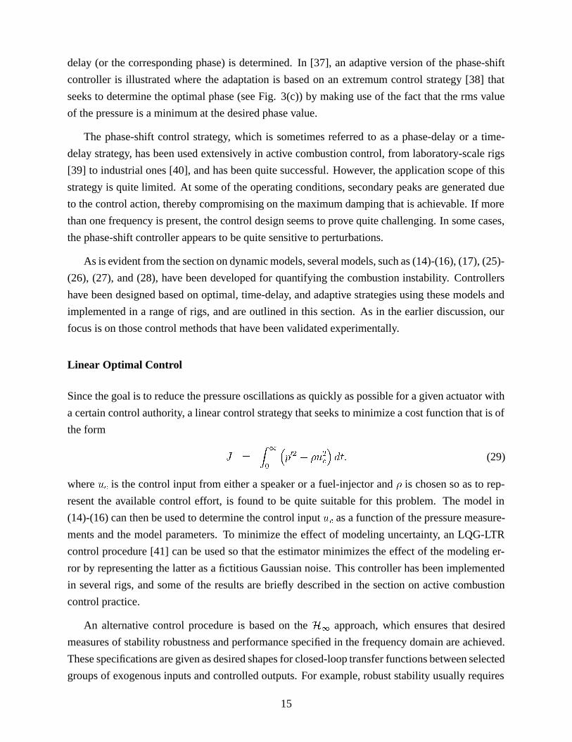
Linear Optimal Control

Since the goal is to reduce the pressure oscillations as quickly as possible for a given actuator with

a certain control authority, a linear control strategy that seeks to minimize a cost function that is of

the form

J =Z1

0

�p02 + �u2c

�dt; (29)

where uc is the control input from either a speaker or a fuel-injector and � is chosen so as to rep-

resent the available control effort, is found to be quite suitable for this problem. The model in

(14)-(16) can then be used to determine the control input uc as a function of the pressure measure-

ments and the model parameters. To minimize the effect of modeling uncertainty, an LQG-LTR

control procedure [41] can be used so that the estimator minimizes the effect of the modeling er-

ror by representing the latter as a fictitious Gaussian noise. This controller has been implemented

in several rigs, and some of the results are briefly described in the section on active combustion

control practice.

An alternative control procedure is based on the H1 approach, which ensures that desired

measures of stability robustness and performance specified in the frequency domain are achieved.

These specifications are given as desired shapes for closed-loop transfer functions between selected

groups of exogenous inputs and controlled outputs. For example, robust stability usually requires

15

the appropriate closed-loop transfer function to be small at high frequencies, as the size of uncer-

tainty is large there. SinceH1-optimal control leads to all-pass closed-loop transfer functions, the

H1 control problem is formulated using frequency-weighted transfer functions. This method has

also been applied for combustion instability using models (25)-(26) in [42] and models of the form

(14)-(16) in [43] and led to satisfactory pressure reduction.

Note that both of the above methods either neglect the effects of time delay or use Pade approx-

imants to represent time-delay effects using a finite-dimensional model, which restricts the domain

of applicability of these controllers to systems where the delay is small.

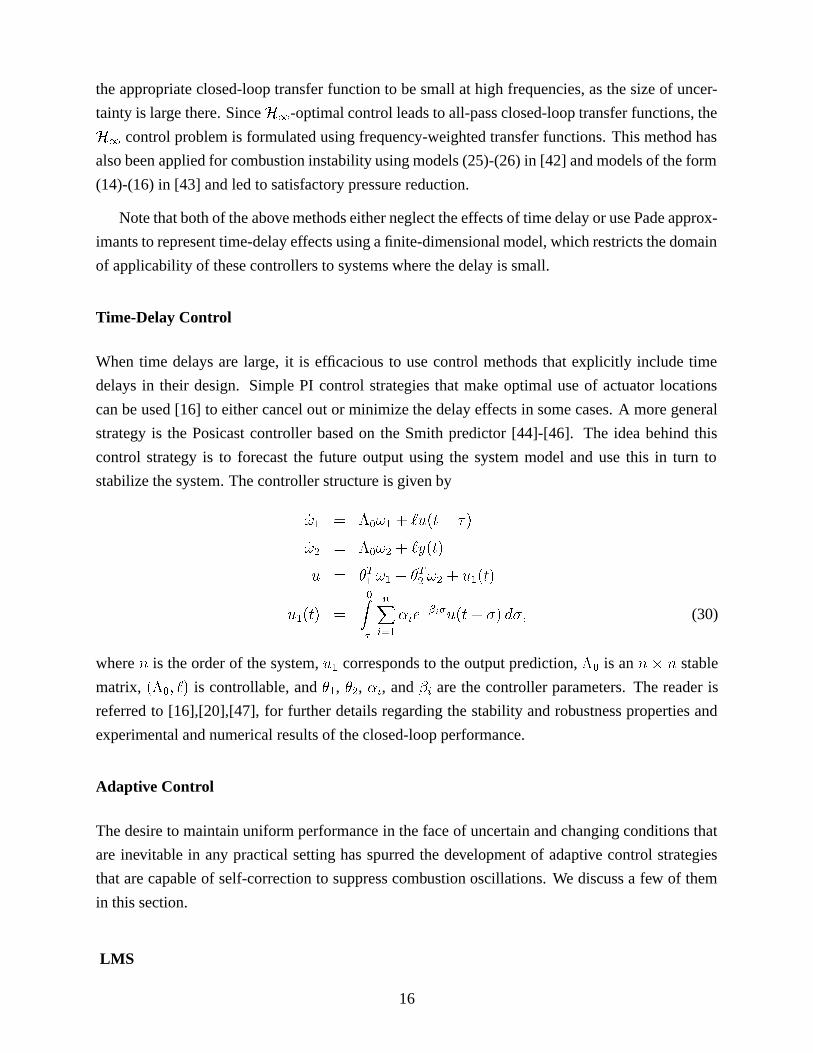
Time-Delay Control

When time delays are large, it is efficacious to use control methods that explicitly include time

delays in their design. Simple PI control strategies that make optimal use of actuator locations

can be used [16] to either cancel out or minimize the delay effects in some cases. A more general

strategy is the Posicast controller based on the Smith predictor [44]-[46]. The idea behind this

control strategy is to forecast the future output using the system model and use this in turn to

stabilize the system. The controller structure is given by

_!1 = �0!1 + `u(t� �)

_!2 = �0!2 + `y(t)

u = �T1!1 + �T

2!2 + u1(t)

u1(t) =

0Z��

nXi=1

�ie��i�u(t+ �) d�; (30)

where n is the order of the system, u1 corresponds to the output prediction, �0 is an n � n stable

matrix, (�0; `) is controllable, and �1, �2, �i, and �i are the controller parameters. The reader is

referred to [16],[20],[47], for further details regarding the stability and robustness properties and

experimental and numerical results of the closed-loop performance.

Adaptive Control

The desire to maintain uniform performance in the face of uncertain and changing conditions that

are inevitable in any practical setting has spurred the development of adaptive control strategies

that are capable of self-correction to suppress combustion oscillations. We discuss a few of them

in this section.

LMS

16

The LMS algorithm [48] consists of deploying an adaptive filter whose coefficients are adjusted so

as to minimize an error that represents a departure from the desired values of a key variable. In the

combustion problem, the underlying model is of the form

p0(i) = W (z)[kTX(i)]; (31)

where W (z) represents the combustion dynamics, X is a signal measured from the controlled

system, and p0 is the unsteady pressure whose desired value is zero. This motivates the filtered-x

LMS algorithm [48] where the update rule is given by

�k(i) = ��p0(i)Xf(i); (32)

where Xf = W (z)[X]. Since W (z) represents either a part of or the complete dynamics of the

combustor, uncertainties in the dynamics also necessitate a parallel identification loop that deter-

mines the parameters of W (z) online. In [49], such a scheme was observed to exhibit instabilities

in the adaptive filter coefficients. In [50], no instabilities were reported, but a second mode was

often excited, sometimes leading to partial extinction in the combustor. It should in fact be noted

that the filtered-x algorithm does not have guaranteed properties of stability and convergence in

general. A modified LMS algorithm was suggested in [51] that resolves many of the shortcomings

observed in [49],[50].

Model-Based Self-Tuning Control

An alternative approach to adaptive control is to exploit the structure of the dynamic model. For

example, for certain actuator locations, the transfer functions corresponding to the models in (14)-

(16) and (25)-(26) can be shown to have relative degree smaller than two, with stable zeros, and

known high-frequency gain. For these cases, a simple adaptive phase-lead compensator can be

shown to successfully suppress the pressure oscillations [20],[52], and is of the form

u = k0(t)p0+

:k0 p

00 (33):k0 = � kp

0p00 (34)

p0 = kcs+ zcs+ pc

[p0]; p00 =1

s+ ap0: (35)

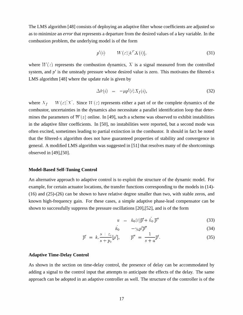
Adaptive Time-Delay Control

As shown in the section on time-delay control, the presence of delay can be accommodated by

adding a signal to the control input that attempts to anticipate the effects of the delay. The same

approach can be adopted in an adaptive controller as well. The structure of the controller is of the

17

same form as in (30), but the parameters �1 and �2 are adjusted online and u1 is chosen as

u1 = �T(t)u(t)

_�(t) = �y(t)!(t� �);

where � = [�T1; �T

2; �

T]T ; ! = [!T

1; !T

2; uT ]T ; ui, the ith element of the vector u(t), is the ith

sample of u(t) in the interval [t� �; t), i = 1; : : : ; p; and p is chosen to be small enough so that the

sampling error in the realization of u1 is small. The stability of the above controller is discussed

in [47]. A controller whose order depended on the relative degree of the plant rather than its own

order was developed in [53] and successfully implemented on a benchtop combustor in [20].

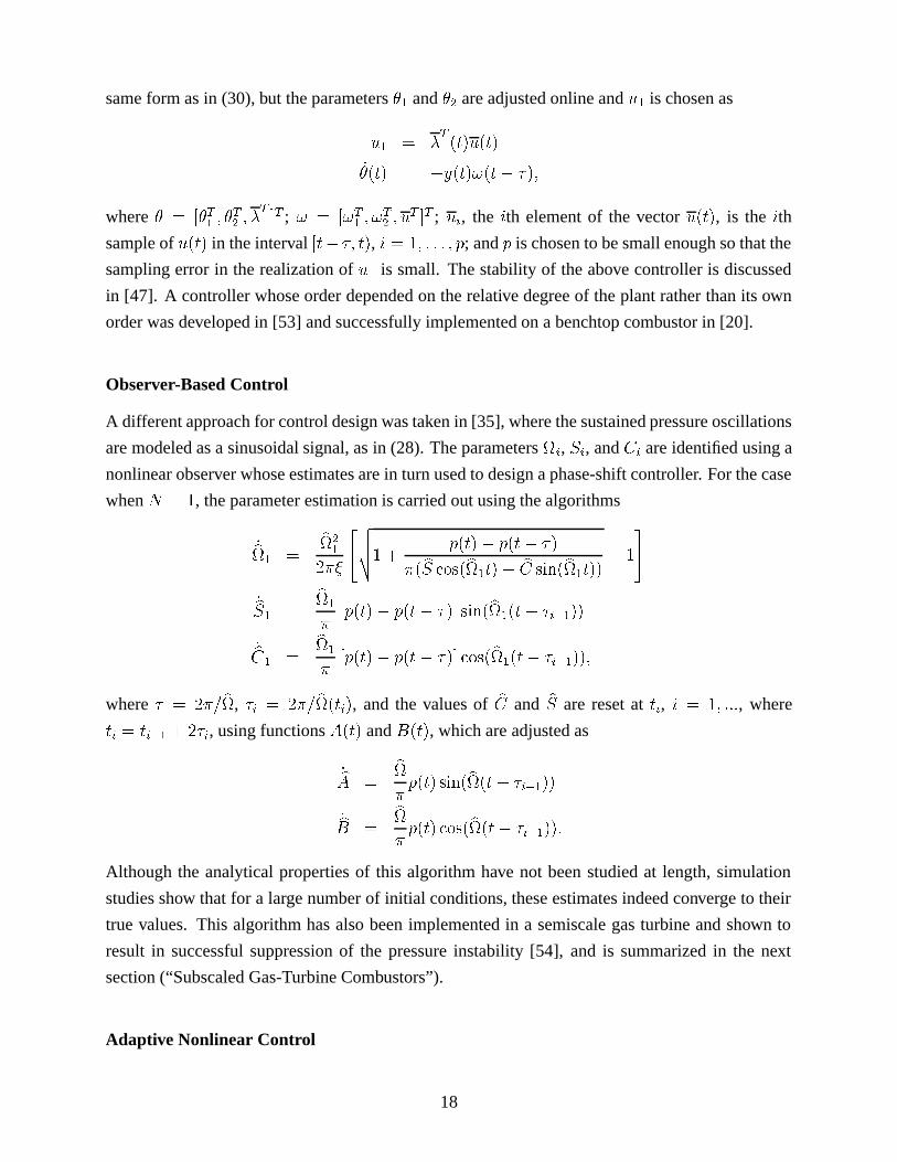
Observer-Based Control

A different approach for control design was taken in [35], where the sustained pressure oscillations

are modeled as a sinusoidal signal, as in (28). The parameters i, Si, and Ci are identified using a

nonlinear observer whose estimates are in turn used to design a phase-shift controller. For the case

when N = 1, the parameter estimation is carried out using the algorithms

_b1 =b2

1

2��

24vuut1 +p(t)� p(t� �)

�( bS cos(b1t)� bC sin(b1t))� 1

35_bS1 =

b1

�[p(t)� p(t� �)] sin(b1(t� �i�1))

_bC1 =b1

�[p(t)� p(t� �)] cos(b1(t� �i�1));

where � = 2�=b, �i = 2�=b(ti), and the values of bC and bS are reset at ti, i = 1; :::, where

ti = ti�1 + 2�i, using functions A(t) and B(t), which are adjusted as

_bA =b�p(t) sin(b(t� �i�1))

_bB =b�p(t) cos(b(t� �i�1)):

Although the analytical properties of this algorithm have not been studied at length, simulation

studies show that for a large number of initial conditions, these estimates indeed converge to their

true values. This algorithm has also been implemented in a semiscale gas turbine and shown to

result in successful suppression of the pressure instability [54], and is summarized in the next

section (“Subscaled Gas-Turbine Combustors”).

Adaptive Nonlinear Control

18

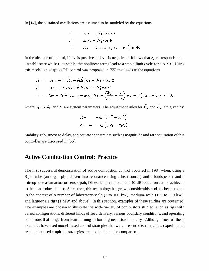
In [14], the sustained oscillations are assumed to be modeled by the equations

_r1 = �c1r1 � �r1r2 cos �

_r2 = �c2r2 � �r21cos �

_� = 2�c1 � �c2 � ���c2

1r2 � 2r2

�sin�:

In the absence of control, if �c1 is positive and �c2 is negative, it follows that r1 corresponds to an

unstable state while r2 is stable; the nonlinear terms lead to a stable limit cycle for a � > 0. Using

this model, an adaptive PD control was proposed in [55] that leads to the equations

_r1 = �1r1 + ( 1cKd + Æ1cKp)r1 � �r1r2 cos �

_r2 = �2r2 + ( 2cKd + Æ2cKp)r2 � �r21cos �

_� = 2�1 � �2 + (2!1Æ1 � !2Æ2)cKD �

�2 1!� 2!2

� cKP � ���c2

1r2 � 2r2

�sin�;

where 1, 2, Æ1, and Æ2 are system parameters. The adjustment rules for cKp and cKD are given by

_KP = �gP�Æ1r

2

1+ Æ2r

2

2

�_KD = �gD

� 1r

2

1+ 2r

2

2

�:

Stability, robustness to delay, and actuator constraints such as magnitude and rate saturation of this

controller are discussed in [55].

Active Combustion Control: Practice

The first successful demonstration of active combustion control occurred in 1984 when, using a

Rijke tube (an organ pipe driven into resonance using a heat source) and a loudspeaker and a

microphone as an actuator-sensor pair, Dines demonstrated that a 40-dB reduction can be achieved

in the heat-induced noise. Since then, this technology has grown considerably and has been studied

in the context of a number of laboratory-scale (1 to 100 kW), medium-scale (100 to 500 kW),

and large-scale rigs (1 MW and above). In this section, examples of these studies are presented.

The examples are chosen to illustrate the wide variety of combustors studied, such as rigs with

varied configurations, different kinds of feed delivery, various boundary conditions, and operating

conditions that range from lean burning to burning near stoichiometry. Although most of these

examples have used model-based control strategies that were presented earlier, a few experimental

results that used empirical strategies are also included for comparison.

19

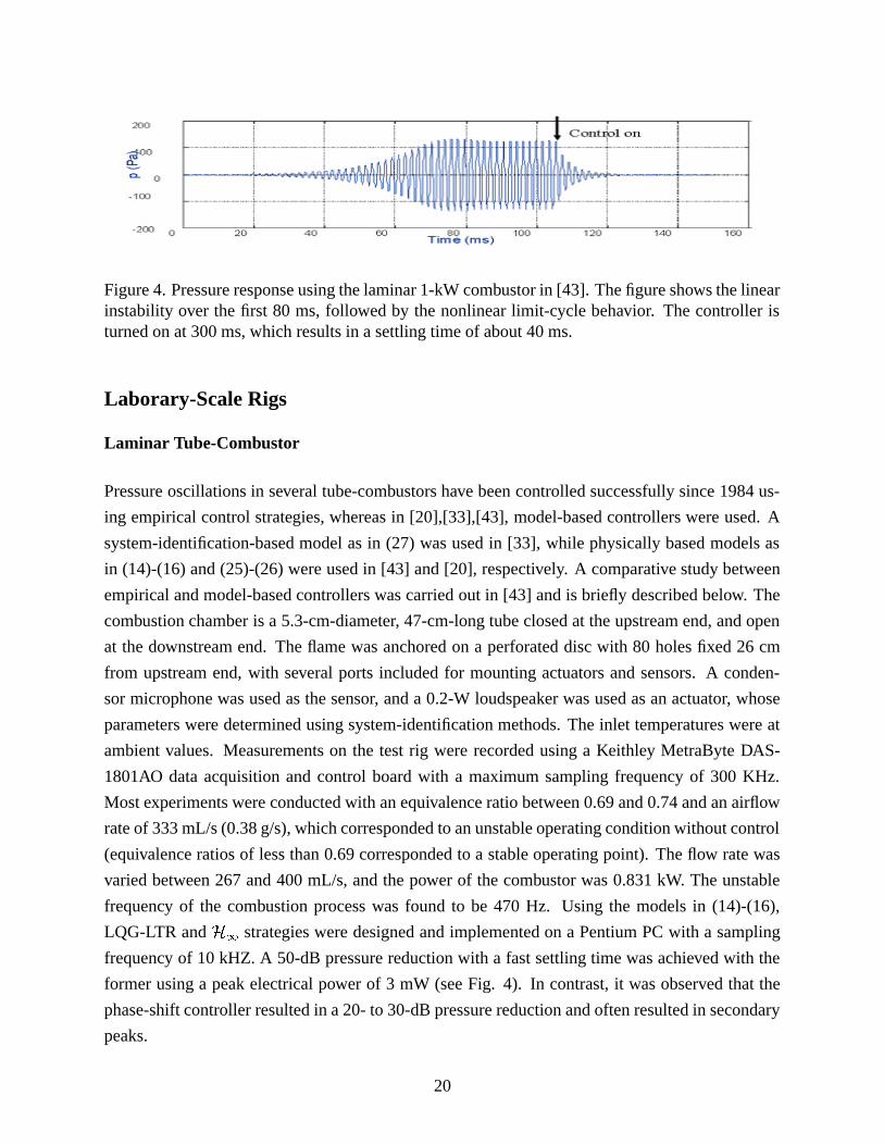
Figure 4. Pressure response using the laminar 1-kW combustor in [43]. The figure shows the linearinstability over the first 80 ms, followed by the nonlinear limit-cycle behavior. The controller isturned on at 300 ms, which results in a settling time of about 40 ms.

Laborary-Scale Rigs

Laminar Tube-Combustor

Pressure oscillations in several tube-combustors have been controlled successfully since 1984 us-

ing empirical control strategies, whereas in [20],[33],[43], model-based controllers were used. A

system-identification-based model as in (27) was used in [33], while physically based models as

in (14)-(16) and (25)-(26) were used in [43] and [20], respectively. A comparative study between

empirical and model-based controllers was carried out in [43] and is briefly described below. The

combustion chamber is a 5.3-cm-diameter, 47-cm-long tube closed at the upstream end, and open

at the downstream end. The flame was anchored on a perforated disc with 80 holes fixed 26 cm

from upstream end, with several ports included for mounting actuators and sensors. A conden-

sor microphone was used as the sensor, and a 0.2-W loudspeaker was used as an actuator, whose

parameters were determined using system-identification methods. The inlet temperatures were at

ambient values. Measurements on the test rig were recorded using a Keithley MetraByte DAS-

1801AO data acquisition and control board with a maximum sampling frequency of 300 KHz.

Most experiments were conducted with an equivalence ratio between 0.69 and 0.74 and an airflow

rate of 333 mL/s (0.38 g/s), which corresponded to an unstable operating condition without control

(equivalence ratios of less than 0.69 corresponded to a stable operating point). The flow rate was

varied between 267 and 400 mL/s, and the power of the combustor was 0.831 kW. The unstable

frequency of the combustion process was found to be 470 Hz. Using the models in (14)-(16),

LQG-LTR and H1 strategies were designed and implemented on a Pentium PC with a sampling

frequency of 10 kHZ. A 50-dB pressure reduction with a fast settling time was achieved with the

former using a peak electrical power of 3 mW (see Fig. 4). In contrast, it was observed that the

phase-shift controller resulted in a 20- to 30-dB pressure reduction and often resulted in secondary

peaks.

20

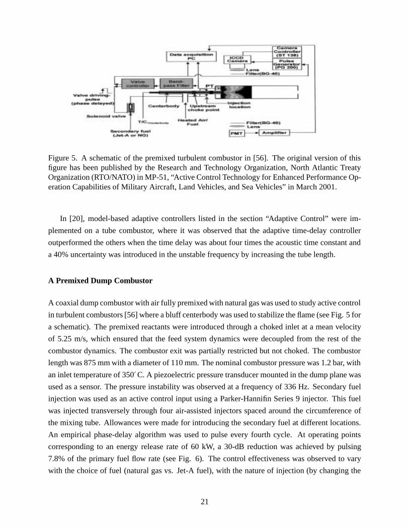
Figure 5. A schematic of the premixed turbulent combustor in [56]. The original version of thisfigure has been published by the Research and Technology Organization, North Atlantic TreatyOrganization (RTO/NATO) in MP-51, “Active Control Technology for Enhanced Performance Op-eration Capabilities of Military Aircraft, Land Vehicles, and Sea Vehicles” in March 2001.

In [20], model-based adaptive controllers listed in the section “Adaptive Control” were im-

plemented on a tube combustor, where it was observed that the adaptive time-delay controller

outperformed the others when the time delay was about four times the acoustic time constant and

a 40% uncertainty was introduced in the unstable frequency by increasing the tube length.

A Premixed Dump Combustor

A coaxial dump combustor with air fully premixed with natural gas was used to study active control

in turbulent combustors [56] where a bluff centerbody was used to stabilize the flame (see Fig. 5 for

a schematic). The premixed reactants were introduced through a choked inlet at a mean velocity

of 5.25 m/s, which ensured that the feed system dynamics were decoupled from the rest of the

combustor dynamics. The combustor exit was partially restricted but not choked. The combustor

length was 875 mm with a diameter of 110 mm. The nominal combustor pressure was 1.2 bar, with

an inlet temperature of 350ÆC. A piezoelectric pressure transducer mounted in the dump plane was

used as a sensor. The pressure instability was observed at a frequency of 336 Hz. Secondary fuel

injection was used as an active control input using a Parker-Hannifin Series 9 injector. This fuel

was injected transversely through four air-assisted injectors spaced around the circumference of

the mixing tube. Allowances were made for introducing the secondary fuel at different locations.

An empirical phase-delay algorithm was used to pulse every fourth cycle. At operating points

corresponding to an energy release rate of 60 kW, a 30-dB reduction was achieved by pulsing

7.8% of the primary fuel flow rate (see Fig. 6). The control effectiveness was observed to vary

with the choice of fuel (natural gas vs. Jet-A fuel), with the nature of injection (by changing the

21

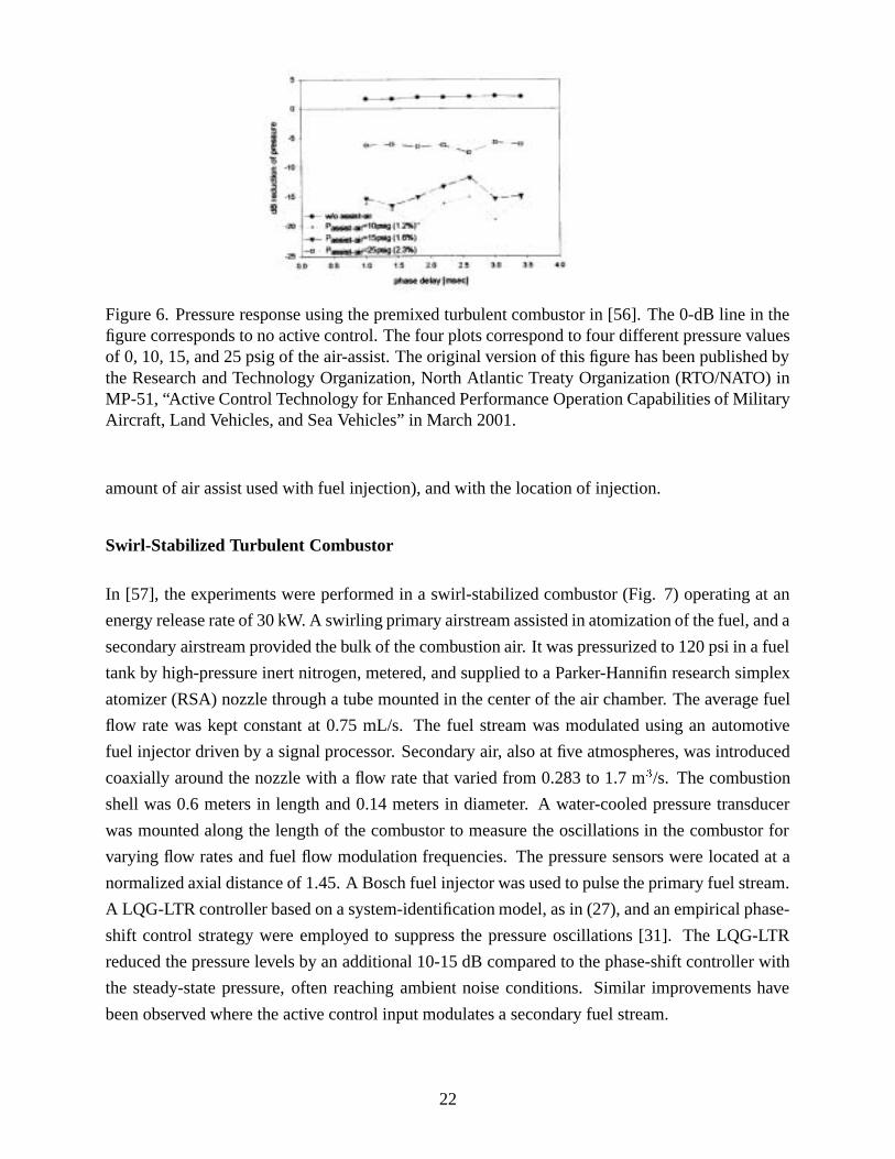
Figure 6. Pressure response using the premixed turbulent combustor in [56]. The 0-dB line in thefigure corresponds to no active control. The four plots correspond to four different pressure valuesof 0, 10, 15, and 25 psig of the air-assist. The original version of this figure has been published bythe Research and Technology Organization, North Atlantic Treaty Organization (RTO/NATO) inMP-51, “Active Control Technology for Enhanced Performance Operation Capabilities of MilitaryAircraft, Land Vehicles, and Sea Vehicles” in March 2001.

amount of air assist used with fuel injection), and with the location of injection.

Swirl-Stabilized Turbulent Combustor

In [57], the experiments were performed in a swirl-stabilized combustor (Fig. 7) operating at an

energy release rate of 30 kW. A swirling primary airstream assisted in atomization of the fuel, and a

secondary airstream provided the bulk of the combustion air. It was pressurized to 120 psi in a fuel

tank by high-pressure inert nitrogen, metered, and supplied to a Parker-Hannifin research simplex

atomizer (RSA) nozzle through a tube mounted in the center of the air chamber. The average fuel

flow rate was kept constant at 0.75 mL/s. The fuel stream was modulated using an automotive

fuel injector driven by a signal processor. Secondary air, also at five atmospheres, was introduced

coaxially around the nozzle with a flow rate that varied from 0.283 to 1.7 m3/s. The combustion

shell was 0.6 meters in length and 0.14 meters in diameter. A water-cooled pressure transducer

was mounted along the length of the combustor to measure the oscillations in the combustor for

varying flow rates and fuel flow modulation frequencies. The pressure sensors were located at a

normalized axial distance of 1.45. A Bosch fuel injector was used to pulse the primary fuel stream.

A LQG-LTR controller based on a system-identification model, as in (27), and an empirical phase-

shift control strategy were employed to suppress the pressure oscillations [31]. The LQG-LTR

reduced the pressure levels by an additional 10-15 dB compared to the phase-shift controller with

the steady-state pressure, often reaching ambient noise conditions. Similar improvements have

been observed where the active control input modulates a secondary fuel stream.

22

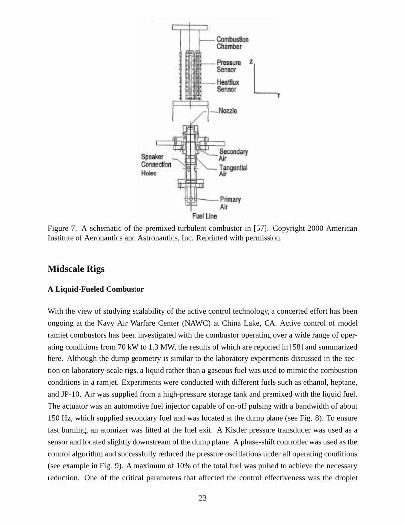
Figure 7. A schematic of the premixed turbulent combustor in [57]. Copyright 2000 AmericanInstitute of Aeronautics and Astronautics, Inc. Reprinted with permission.

Midscale Rigs

A Liquid-Fueled Combustor

With the view of studying scalability of the active control technology, a concerted effort has been

ongoing at the Navy Air Warfare Center (NAWC) at China Lake, CA. Active control of model

ramjet combustors has been investigated with the combustor operating over a wide range of oper-

ating conditions from 70 kW to 1.3 MW, the results of which are reported in [58] and summarized

here. Although the dump geometry is similar to the laboratory experiments discussed in the sec-

tion on laboratory-scale rigs, a liquid rather than a gaseous fuel was used to mimic the combustion

conditions in a ramjet. Experiments were conducted with different fuels such as ethanol, heptane,

and JP-10. Air was supplied from a high-pressure storage tank and premixed with the liquid fuel.

The actuator was an automotive fuel injector capable of on-off pulsing with a bandwidth of about

150 Hz, which supplied secondary fuel and was located at the dump plane (see Fig. 8). To ensure

fast burning, an atomizer was fitted at the fuel exit. A Kistler pressure transducer was used as a

sensor and located slightly downstream of the dump plane. A phase-shift controller was used as the

control algorithm and successfully reduced the pressure oscillations under all operating conditions

(see example in Fig. 9). A maximum of 10% of the total fuel was pulsed to achieve the necessary

reduction. One of the critical parameters that affected the control effectiveness was the droplet

23

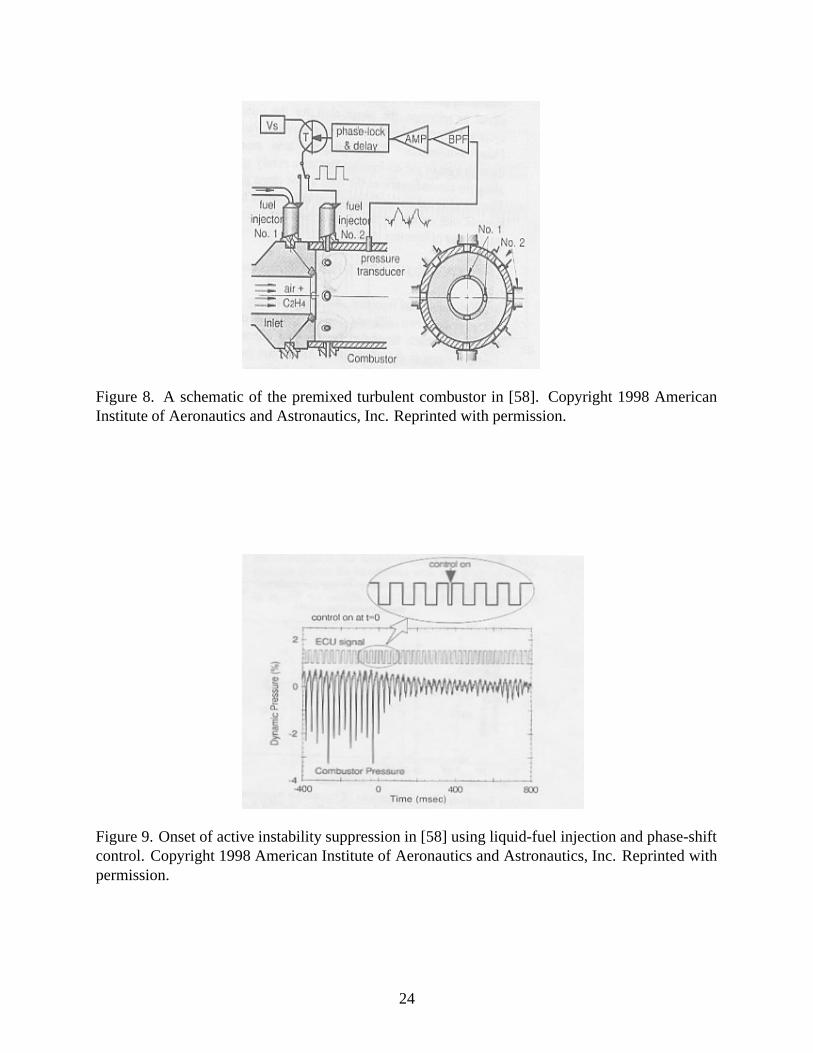
Figure 8. A schematic of the premixed turbulent combustor in [58]. Copyright 1998 AmericanInstitute of Aeronautics and Astronautics, Inc. Reprinted with permission.

Figure 9. Onset of active instability suppression in [58] using liquid-fuel injection and phase-shiftcontrol. Copyright 1998 American Institute of Aeronautics and Astronautics, Inc. Reprinted withpermission.

24

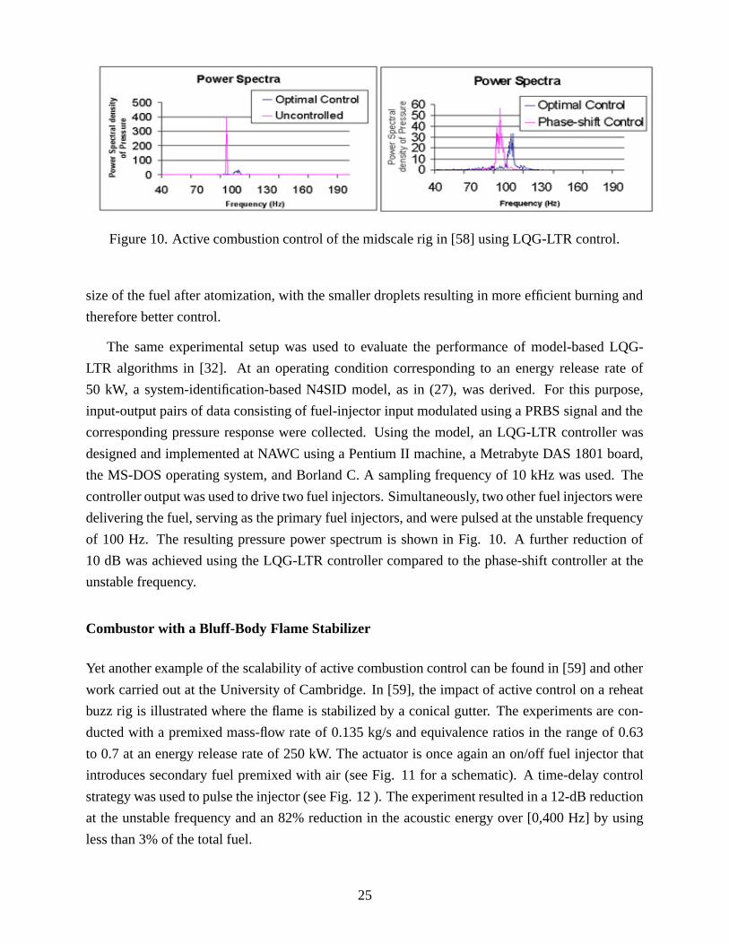
Figure 10. Active combustion control of the midscale rig in [58] using LQG-LTR control.

size of the fuel after atomization, with the smaller droplets resulting in more efficient burning and

therefore better control.

The same experimental setup was used to evaluate the performance of model-based LQG-

LTR algorithms in [32]. At an operating condition corresponding to an energy release rate of

50 kW, a system-identification-based N4SID model, as in (27), was derived. For this purpose,

input-output pairs of data consisting of fuel-injector input modulated using a PRBS signal and the

corresponding pressure response were collected. Using the model, an LQG-LTR controller was

designed and implemented at NAWC using a Pentium II machine, a Metrabyte DAS 1801 board,

the MS-DOS operating system, and Borland C. A sampling frequency of 10 kHz was used. The

controller output was used to drive two fuel injectors. Simultaneously, two other fuel injectors were

delivering the fuel, serving as the primary fuel injectors, and were pulsed at the unstable frequency

of 100 Hz. The resulting pressure power spectrum is shown in Fig. 10. A further reduction of

10 dB was achieved using the LQG-LTR controller compared to the phase-shift controller at the

unstable frequency.

Combustor with a Bluff-Body Flame Stabilizer

Yet another example of the scalability of active combustion control can be found in [59] and other

work carried out at the University of Cambridge. In [59], the impact of active control on a reheat

buzz rig is illustrated where the flame is stabilized by a conical gutter. The experiments are con-

ducted with a premixed mass-flow rate of 0.135 kg/s and equivalence ratios in the range of 0.63

to 0.7 at an energy release rate of 250 kW. The actuator is once again an on/off fuel injector that

introduces secondary fuel premixed with air (see Fig. 11 for a schematic). A time-delay control

strategy was used to pulse the injector (see Fig. 12 ). The experiment resulted in a 12-dB reduction

at the unstable frequency and an 82% reduction in the acoustic energy over [0,400 Hz] by using

less than 3% of the total fuel.

25

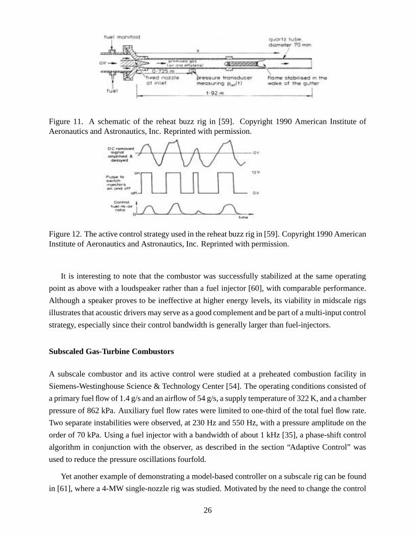
Figure 11. A schematic of the reheat buzz rig in [59]. Copyright 1990 American Institute ofAeronautics and Astronautics, Inc. Reprinted with permission.

Figure 12. The active control strategy used in the reheat buzz rig in [59]. Copyright 1990 AmericanInstitute of Aeronautics and Astronautics, Inc. Reprinted with permission.

It is interesting to note that the combustor was successfully stabilized at the same operating

point as above with a loudspeaker rather than a fuel injector [60], with comparable performance.

Although a speaker proves to be ineffective at higher energy levels, its viability in midscale rigs

illustrates that acoustic drivers may serve as a good complement and be part of a multi-input control

strategy, especially since their control bandwidth is generally larger than fuel-injectors.

Subscaled Gas-Turbine Combustors

A subscale combustor and its active control were studied at a preheated combustion facility in

Siemens-Westinghouse Science & Technology Center [54]. The operating conditions consisted of

a primary fuel flow of 1.4 g/s and an airflow of 54 g/s, a supply temperature of 322 K, and a chamber

pressure of 862 kPa. Auxiliary fuel flow rates were limited to one-third of the total fuel flow rate.

Two separate instabilities were observed, at 230 Hz and 550 Hz, with a pressure amplitude on the

order of 70 kPa. Using a fuel injector with a bandwidth of about 1 kHz [35], a phase-shift control

algorithm in conjunction with the observer, as described in the section “Adaptive Control” was

used to reduce the pressure oscillations fourfold.

Yet another example of demonstrating a model-based controller on a subscale rig can be found

in [61], where a 4-MW single-nozzle rig was studied. Motivated by the need to change the control

26

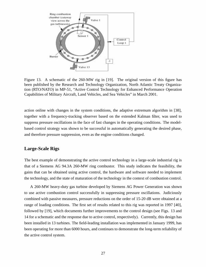
Figure 13. A schematic of the 260-MW rig in [19]. The original version of this figure hasbeen published by the Research and Technology Organization, North Atlantic Treaty Organiza-tion (RTO/NATO) in MP-51, “Active Control Technology for Enhanced Performance OperationCapabilities of Military Aircraft, Land Vehicles, and Sea Vehicles” in March 2001.

action online with changes in the system conditions, the adaptive extremum algorithm in [38],

together with a frequency-tracking observer based on the extended Kalman filter, was used to

suppress pressure oscillations in the face of fast changes in the operating conditions. The model-

based control strategy was shown to be successful in automatically generating the desired phase,

and therefore pressure suppression, even as the engine conditions changed.

Large-Scale Rigs

The best example of demonstrating the active control technology in a large-scale industrial rig is

that of a Siemens AG 94.3A 260-MW ring combustor. This study indicates the feasibility, the

gains that can be obtained using active control, the hardware and software needed to implement

the technology, and the state of maturation of the technology in the context of combustion control.

A 260-MW heavy-duty gas turbine developed by Siemens AG Power Generation was shown

to use active combustion control successfully in suppressing pressure oscillations. Judiciously

combined with passive measures, pressure reductions on the order of 15-20 dB were obtained at a

range of loading conditions. The first set of results related to this rig was reported in 1997 [40],

followed by [19], which documents further improvements to the control design (see Figs. 13 and

14 for a schematic and the response due to active control, respectively). Currently, this design has

been installed in 13 turbines. The field-leading installation was implemented in January 1999, has

been operating for more than 6000 hours, and continues to demonstrate the long-term reliability of

the active control system.

27

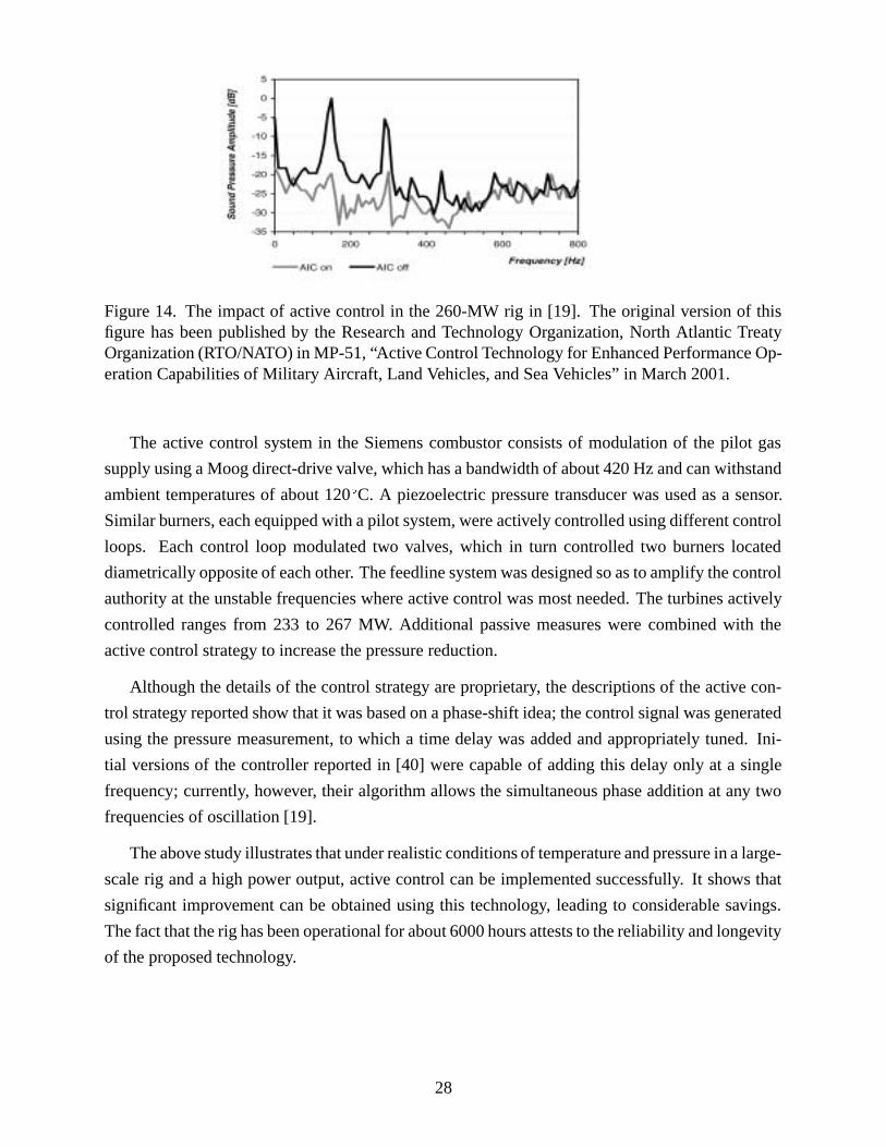
Figure 14. The impact of active control in the 260-MW rig in [19]. The original version of thisfigure has been published by the Research and Technology Organization, North Atlantic TreatyOrganization (RTO/NATO) in MP-51, “Active Control Technology for Enhanced Performance Op-eration Capabilities of Military Aircraft, Land Vehicles, and Sea Vehicles” in March 2001.

The active control system in the Siemens combustor consists of modulation of the pilot gas

supply using a Moog direct-drive valve, which has a bandwidth of about 420 Hz and can withstand

ambient temperatures of about 120ÆC. A piezoelectric pressure transducer was used as a sensor.

Similar burners, each equipped with a pilot system, were actively controlled using different control

loops. Each control loop modulated two valves, which in turn controlled two burners located

diametrically opposite of each other. The feedline system was designed so as to amplify the control

authority at the unstable frequencies where active control was most needed. The turbines actively

controlled ranges from 233 to 267 MW. Additional passive measures were combined with the

active control strategy to increase the pressure reduction.

Although the details of the control strategy are proprietary, the descriptions of the active con-

trol strategy reported show that it was based on a phase-shift idea; the control signal was generated

using the pressure measurement, to which a time delay was added and appropriately tuned. Ini-

tial versions of the controller reported in [40] were capable of adding this delay only at a single

frequency; currently, however, their algorithm allows the simultaneous phase addition at any two

frequencies of oscillation [19].

The above study illustrates that under realistic conditions of temperature and pressure in a large-

scale rig and a high power output, active control can be implemented successfully. It shows that

significant improvement can be obtained using this technology, leading to considerable savings.

The fact that the rig has been operational for about 6000 hours attests to the reliability and longevity

of the proposed technology.

28

Summary

The overarching consensus in the field is that active combustion control is a viable and feasible

technology. The best illustration of this technology is that of Siemens-Westinghouse Inc. on a

264-MW annular rig. The demonstrations by United Technologies Research Center on a single-

nozzle rig [61],[62] and that of Siemens-Westinghouse in [54] indicate the range of geometries

where comparable gains have been realized.

Modeling of combustion instability has come a long way. The main challenge in this area is the

characterization of unsteady heat-release dynamics and the instigating mechanisms that produce

unsteadiness. Under suitable simplifications, these mechanisms are beginning to be understood and

modeled. Even with the resulting low-order time-delay models, instability behavior in a number

of rigs has been explained. The next major hurdle is the study of flame dynamics under turbulent

conditions where flame-vortex interactions are significant.

Model-based control strategies are beginning to play a role in this field and are being im-

plemented in recent years with clear evidence of the gains that can be realized over phase-shift

controllers. The underlying models represent a class of time-delay systems, thereby dictating the

development of suitable time-delay controllers; the system uncertainties present have led to the

derivation of adaptive controllers that guarantee satisfactory performance in the presence of large

delays.

Despite the above success, several issues remain to be addressed. In cases where active control

resulted in a clear improvement, what the contributing factors were that led to such a performance

is not well understood. The overall closed-loop combustor needs to be optimized to achieve better

quality, reliability, and repeatability at lower cost, as well as better speeds. Uniformity in perfor-

mance needs to be realized over a large range of flow rates and loads in the presence of chemical,

hydrodynamic, and acoustic uncertainties.

Combustion instability suppression is but one objective of combustion control. Maintaining

high premixedness, low NOx levels, complete combustion, and control of pattern factor, as well as

enhancing the flammability limits and increasing the volumetric heat-release rate, are other typical

and often concomitant requirements in applications such as gas turbines, afterburners, and ramjet

engines. To realize these multiple performance objectives, a systems study of analysis and syn-

thesis needs to be carried out. This requires the judicious use of multiple, distributed, and varying

types of actuators located at various points in the combustion chamber. Development of hierar-

chical control architectures that address the multiple time scales in the problem and accommodate

variations in the system, environment, and operating conditions are necessary directions for current

and future research.

29

Acknowledgments

This work is sponsored in part by the National Science Foundation, contract no. ECS 9713415,and in part by the Office of Naval Research, contract no. N00014-99-1-0448.

References

[1] J.W.S. Rayleigh, The Theory of Sound, volume 2. New York: Dover, 1945.

[2] B.T. Chu, “Stability of systems containing a heat source–The Rayleigh criterion,” technical report,NASA Research Memorandum RN 56D27, 1956.

[3] A.A. Putnam, Combustion Driven Oscillations in Industry. New York: American Elsevier Pub. Co.,1971.

[4] A.M. Annaswamy, “Nonlinear modeling and control of combustion dynamics,” in Fluid Flow Control(in press), P. Koumoutsakos, I. Mezic, and M. Morari, eds, New York: Springer Verlag, 2002.

[5] S. Candel, D. Thevenin, N. Darabiha, and D. Veynante, “Progress in numerical combustion,” Com-bustion Science and Technology, vol.149, pp.297–337, 1999.

[6] F.E.C. Culick, “Combustion instabilities in liquid-fueled propulsion systems - An Overview,” inAGARD Conference Proceedings, paper 1, 450, The 72

nd(B) Propulsion and Energetics Panel Spe-cialists Meeting, 1988.

[7] M. Fleifil, A.M. Annaswamy, Z. Ghoniem, and A.F. Ghoniem, “Response of a laminar premixed flameto flow oscillations: A kinematic model and thermoacoustic instability result,” Combustion and Flame,vol.106, pp.487–510, 1996.

[8] A.A. Peracchio and W. Proscia, “Nonlinear heat release/acoustic model for thermoacoustic instabilityin lean premixed combustors,” in ASME Gas Turbine and Aerospace Congress, Stockholm, Sweden,1998.

[9] A.P. Dowling, “A kinematic model of of a ducted flame,” Journal of Fluid Mechanics, vol.394,pp.51–72, 1999.

[10] T. Lieuwen and B.T. Zinn, “The role of equivalence ratio oscillations in driving combustion instabil-ities in low N0x gas turbines,” The Twenty-Seventh International Symposium on Combustion, 1998,pp.1809–1816.

[11] S. Park, A.M. Annaswamy, and A.F. Ghoniem, “Heat release dynamics modeling of kinetically con-trolled burning,” Combustion and Flame, vol.128, pp.217–231, 2002.

[12] S. Turns, Introduction to Combustion. New York: McGraw-Hill, 1996.

[13] B.T. Zinn and M.E. Lores, “Application of the galerkin method in the solution of nonlinear axial com-bustion instability problems in liquid rockets,” Combustion Science and Technology, vol.4, pp.269–278, 1972.

[14] F.E.C. Culick, “Nonlinear behavior of acoustic waves in combustion chambers,” Acta Astronautica,vol.3, pp.715–756, 1976.

30

[15] A.M. Annaswamy, M. Fleifil, J.P. Hathout, and A.F. Ghoniem, “Impact of linear coupling on the designof active controllers for thermoacoustic instability,” Combustion Science and Technology, vol.128,pp.131–180, 1997.

[16] J.P. Hathout, M. Fleifil, A.M. Annaswamy, and A.F. Ghoniem, “Active control of combustion insta-bility using fuel-injection in the presence of time-delays,” AIAA Journal of Propulsion and Power (inpress), 2002.

[17] M. Fleifil, J.P. Hathout, A.M. Annaswamy, and A.F. Ghoniem, “The origin of secondary peaks withactive control of thermoacoustic instability,” Combustion Science and Technology, vol.133, pp.227–265, 1998.

[18] K. Ogata, Modern Control Engineering. third edition, Englewood Cliffs, NJ:Prentice Hall, 1997.

[19] J. Hermann, A. Orthmann, S. Hoffmann, and P. Berenbrink, “Combination of active instability controland passive measures to prevent combustion instabilities in a 260 mw heavy duty gas turbine,” inNATO RTO/AVT Symposium on Active Control Technology for Enhanced Performance in Land, Air,and Sea Vehicles, Braunschweig, Germany, May 2000.

[20] S. Evesque, Adaptive Control of Combustion Oscillations, Ph.D. thesis, University of Cambridge,Cambridge, U.K., November 2000.

[21] A.P. Dowling, “Nonlinear self-excited oscillations of a ducted flame,” Journal of Fluid Mechanics,vol.346, pp.271–290, 1999.

[22] M. Fleifil, A.M. Annaswamy, and A.F. Ghoniem, “A physically based nonlinear model of combustioninstability and active control,” in Proceedings of the Conference on Control Applications, Trieste, Italy,August 1998.

[23] J. Rumsey, M. Fleifil, A.M. Annaswamy, J.P. Hathout, and A.F. Ghoniem, “Low-order nonlinear mod-els of thermoacoustic instabilities and linear model-based control,” in Proceedings of the Conferenceon Control Applications, Trieste, Italy, August 1998.

[24] T. Lieuwen and B.T. Zinn, “Experimental investigation of limit cycle oscillations in an unstable gasturbine combustor,” in AIAA 2000-0707, 38th AIAA Aerospace Sciences Meeting, Reno, NV, January2000.

[25] V. Yang and F.E.C. Culick, “Nonlinear analysis of pressure oscillations in ramjet engines,” AIAA-86-0001, 1986.

[26] F.E.C. Culick, “Some recent results for nonlinear acoustics in combustion chambers,” AIAA, vol.32,pp.146–169, 1994.

[27] G. Isella, C. Seywert, F.E.C. Culick, and E. E. Zukoski, “A further note on active control of combustioninstabilities based on hysteresis,” Short Communication, Combustion Science and Technology, vol.126,pp.381–388, 1997.

[28] G.A. Richards, M.C. Yip, and E.H. Rawlins, “Control of flame oscillations with equivalence ratiomodulation,” Journal of Propulsion and Power, vol.15, pp.232–240, 1999.

[29] R. Prasanth, A.M. Annaswamy, J.P. Hathout, and A.F. Ghoniem, “When do open-loop strategies forcombustion control work?” AIAA Journal of Propulsion and Power (in press), 2002.

[30] L. Ljung and T. Soderstrom, Theory and Practice of Recursive Identification. MA: MIT Press, Cam-bridge, 1985.

31

[31] S. Murugappan, S. Park, A.M. Annaswamy, A.F. Ghoniem, S. Acharya and T. Allgood, “Optimalcontrol of a swirl stabilized spray combustor using system identification approach,” in 38th AIAAAerospace Sciences Meeting and Exhibit, Reno, NV, 2001.

[32] B.J. Brunell, “A system identification approach to active control of thermoacoustic instabilities,”master’s thesis, Department of Mechanical Engineering, MIT, Cambridge, MA, 1996.

[33] J.E. Tierno and J.C. Doyle, “Multimode active stabilization of a Rijke tube,” in DSC-Vol. 38, ASMEWinter Annual Meeting, 1992.

[34] P. van Overschee and B. de Moor, “N4SID: Subspace algorithms for the identification of combineddeterministic-stochastic systems,” Automatica, vol.30, no.1, pp.75–93, 1994.

[35] Y. Neumeier, N. Markopoulos, and B.T. Zinn, “A procedure for real-time mode decomposition, ob-servation, and prediction for active control of combustion instabilities,” in Proceedings of the IEEEConference on Control Applications, Hartford, CT, 1997.

[36] R.M. Murray, C.A. Jacobson, R. Casas, A.I. Khibnik, C.R. Johnson, Jr., R. Bitmead, A.A. Peracchio,and W.M. Proscia, “System identification for limit cycling systems: A case study for combustioninstabilities,” in American Control Conference, Philadelphia, PA, 1998.

[37] S. Murugappan, E.J. Gutmark, S. Acharya, and M.Krstic, “Extremum seeking adaptive controller forswirl stabilized spray combustion,” Twenty-Eighth International Combustion Symposium, Edinburgh,U.K., July 2000.

[38] M. Krstic, Performance improvement and limitations in extremum seeking control, Systems andControl Letters, vol.39, pp.313–326, 2000.

[39] M.A. Heckl, Active control of the noise from a Rijke tube, in Aero- and Hydro-Acoustics, G. Comte-Bellot and J.E. Flowers Williams, eds, pp.211–216, Berlin, Heidelberg:Springer, 1986.

[40] J.R. Seume, N. Vortmeyer, W. Krause, J. Hermann, C.-C Hantschk, P. Zangl, S. Gleis, and D. Vort-meyer, “Application of active combustion instability control to a heavy-duty gas turbine,” in Proceed-ings of the ASME-ASIA, Singapore, 1997.

[41] G. Stein and M. Athans, “The LQG/LTR procedure for multivariable feedback control design,” IEEETransactions on Automatic Control, vol.32, pp.105–114, 1987.

[42] Y.C. Chu, A.P. Dowling, and K. Glover, “Robust control of combustion oscillations,” in Proceedingsof the Conference on Control Applications, Trieste, Italy, August 1998.

[43] A.M. Annaswamy, M. Fleifil, J. Rumsey, J.P. Hathout, R. Prasanth, and A.F. Ghoniem, “Thermoacous-tic instability: Model-based optimal control designs and experimental validation,” IEEE Transactionson Control Systems Technology, vol.8, no.6, pp.905–918, November 2000.

[44] O.J. Smith, “A controller to overcome dead time,” ISA Journal, vol.6, 1959.

[45] A.Z. Manitius and A.W. Olbrot, “Finite spectrum assignement problem for systems with delays,” IEEETransactions on Automatic Control, vol.AC-24, no. 4, 1979.

[46] K. Ichikawa, “Frequency-domain pole assignement and exact model-matching for delay systems,” Int.J. Control, vol.41, pp.1015–1024, 1985.

[47] S. Niculescu and A.M. Annaswamy, “A simple adaptive controller for positive-real systems withtime-delay,” in The American Controller Conference, Chicago, IL, 2000.

32

[48] B. Widrow and S.D. Stearns, Adaptive Signal Processing. Englewood Cliffs, NJ:Prentice-Hall, 1985.

[49] A. Kemal and C.T. Bowman, “Active adaptive control of combustion,” in Proceedings of the IEEEConference on Control Applications, pp. 667–672, Albany, NY, 1995.

[50] G. Billoud, M.A. Galland, C. Huynh Huu, and S. Candel, “Adaptive active control of combustioninstabilities,” Combustion Science and Technology, vol. 81, pp.257–283, 1992.

[51] S. Evesque and A.P. Dowling, “LMS algorithm for adaptive control of combustion oscillations,” Com-bustion Science and Technology, vol.164, pp.65–94, 2001.

[52] A.M. Annaswamy, O. El-Rifai, M. Fleifil, and A.F. Ghoniem, “A model-based self-tuning controllerfor thermoacoustic instability,” Combustion Science and Technology, vol.135, pp.213–240, 1998.

[53] S. Evesque, A.P. Dowling, and A.M. Annaswamy, “Adaptive algorithms for control of combustion,”in NATO RTO/AVT Symposium on Active Control Technology for Enhanced Performance in Land, Air,and Sea Vehicles, Braunschweig, Germany, May 2000.

[54] S.S. Sattinger, Y. Neumeier, A. Nabi, B.T. Zinn, D.J. Amos, and D.D. Darling, “Sub-scale demon-stration of the active feedback control of gas-turbine combustion instabilities,” ASME Journal ofEngineering for Gas Turbines and Power, vol.122, pp.262–268, 2000.

[55] M. Krstic, A.S. Krupadanam, and C. Jacobson, “Self-tuning control of a nonlinear model of combus-tion instabilities,” IEEE Control System Thechnology, vol.7, no.4, pp.424–436, July 1999.

[56] K. Kim, J. Lee, Jacob Stenzler, and D.A. Santavicca, “Optimization of active control systems forsuppressing combustion dynamics,” in NATO RTO/AVT Symposium on Active Control Technology forEnhanced Performance in Land, Air, and Sea Vehicles, Braunschweig, Germany, May 2000.

[57] S. Murugappan, E. Gutmark, and S. Acharya, “Application of extremum seeking controller for sup-pression of combustion instabilities in spray combustion,” AIAA-2000-1025, 38th AIAA AerospaceSciences Meeting, Reno, NV, 2000.

[58] K. Yu, K.J. Wilson, and K.C. Schadow, “Scale-up experiments on liquid-fueled active combustioncontrol,” in 34th AIAA/ASME/SAE/ASEE Joint Propulsion Conference, AIAA 98-3211, Cleveland,OH, 1998.

[59] P.J. Langhorne, A.P. Dowling, and N. Hooper, “Practical active control system for combustion oscil-lations,” Journal of Propulsion and Power, vol.6, no.3, pp.324–333, 1990.

[60] G.J. Bloxsidge, A.P. Dowling, N. Hooper, and P.J. Langhorne, “Active control of reheat buzz,” AIAAJournal, vol.26, no.7, July 1988.

[61] A. Banaszuk, Y. Zhang, and C. Jacobson, “Active control of combustion instabilities in gas turbineengines for low emissions,” Part II: Adaptive control algorithm development, demonstration and per-formance limitations,” in NATO RTO/AVT Symposium on Active Control Technology for EnhancedPerformance in Land, Air, and Sea Vehicles, Braunschweig, Germany, May 2000.

[62] J.M. Cohen, N.M. Rey, C.A. Jacobson, and T.J. Anderson, “Active control of combustion instabilityin a liquid-fueled low-NOx combustor,” ASME 98-GT-267, ASME/IGTI, Sweden, 1998.

33

List of Figures

1 Thermoacoustic instability in a combustion system. . . . . . . . . . . . . . . . . . 2

2 Interacting mechanisms that lead to thermoacoustic instability. p: pressure, u: ve-

locity, q: heat-release rate, T : temperature; A: flame surface area, �: equivalence

ratio, �j: jet velocity, �v: vaporization time-delay, �v: convective delay, d: size of

droplets. . . . . . . . . . . . . . . . . . . . . . . . . . . . . . . . . . . . . . . . . 3

3 (a) A schematic of a phase-shift controller. (b) Pressure response using the phase-

shift controller in the swirl-stabilized rig in [37]. The change in the rms value

with the controller phase is indicated. (c) Response of a self-tuning phase-shift

controller based on an extremum control strategy. Reprinted with permission from

the Combustion Institute. . . . . . . . . . . . . . . . . . . . . . . . . . . . . . . . 14

4 Pressure response using the laminar 1-kW combustor in [43]. The figure shows

the linear instability over the first 80 ms, followed by the nonlinear limit-cycle

behavior. The controller is turned on at 300 ms, which results in a settling time of

about 40 ms. . . . . . . . . . . . . . . . . . . . . . . . . . . . . . . . . . . . . . . 20

5 A schematic of the premixed turbulent combustor in [56]. The original version

of this figure has been published by the Research and Technology Organization,

North Atlantic Treaty Organization (RTO/NATO) in MP-51, “Active Control Tech-

nology for Enhanced Performance Operation Capabilities of Military Aircraft,

Land Vehicles, and Sea Vehicles” in March 2001. . . . . . . . . . . . . . . . . . . 21

6 Pressure response using the premixed turbulent combustor in [56]. The 0-dB line

in the figure corresponds to no active control. The four plots correspond to four

different pressure values of 0, 10, 15, and 25 psig of the air-assist. The original

version of this figure has been published by the Research and Technology Or-

ganization, North Atlantic Treaty Organization (RTO/NATO) in MP-51, “Active

Control Technology for Enhanced Performance Operation Capabilities of Military

Aircraft, Land Vehicles, and Sea Vehicles” in March 2001. . . . . . . . . . . . . . 22

7 A schematic of the premixed turbulent combustor in [57]. Copyright 2000 Ameri-

can Institute of Aeronautics and Astronautics, Inc. Reprinted with permission. . . . 23

8 A schematic of the premixed turbulent combustor in [58]. Copyright 1998 Ameri-

can Institute of Aeronautics and Astronautics, Inc. Reprinted with permission. . . . 24

9 Onset of active instability suppression in [58] using liquid-fuel injection and phase-

shift control. Copyright 1998 American Institute of Aeronautics and Astronautics,

Inc. Reprinted with permission. . . . . . . . . . . . . . . . . . . . . . . . . . . . . 24

10 Active combustion control of the midscale rig in [58] using LQG-LTR control. . . 25

11 A schematic of the reheat buzz rig in [59]. Copyright 1990 American Institute of

Aeronautics and Astronautics, Inc. Reprinted with permission. . . . . . . . . . . . 26

12 The active control strategy used in the reheat buzz rig in [59]. Copyright 1990

American Institute of Aeronautics and Astronautics, Inc. Reprinted with permission. 26

13 A schematic of the 260-MW rig in [19]. The original version of this figure has been

published by the Research and Technology Organization, North Atlantic Treaty

Organization (RTO/NATO) in MP-51, “Active Control Technology for Enhanced

Performance Operation Capabilities of Military Aircraft, Land Vehicles, and Sea

Vehicles” in March 2001. . . . . . . . . . . . . . . . . . . . . . . . . . . . . . . 27

14 The impact of active control in the 260-MW rig in [19]. The original version of this

figure has been published by the Research and Technology Organization, North

Atlantic Treaty Organization (RTO/NATO) in MP-51, “Active Control Technol-

ogy for Enhanced Performance Operation Capabilities of Military Aircraft, Land

Vehicles, and Sea Vehicles” in March 2001. . . . . . . . . . . . . . . . . . . . . . 28

1 Thermoacoustic instability in a combustion system. . . . . . . . . . . . . . . . . . 1

2 Interacting mechanisms that lead to thermoacoustic instability. p: pressure, u: ve-

locity, q: heat-release rate, T : temperature; A: flame surface area, �: equivalence

ratio, �j: jet velocity, �v: vaporization time-delay, �v: convective delay, d: size of

droplets. . . . . . . . . . . . . . . . . . . . . . . . . . . . . . . . . . . . . . . . . 1

3 (a) A schematic of a phase-shift controller. (b) Pressure response using the phase-

shift controller in the swirl-stabilized rig in [37]. The change in the rms value

with the controller phase is indicated. (c) Response of a self-tuning phase-shift

controller based on an extremum control strategy. Reprinted with permission from

the Combustion Institute. . . . . . . . . . . . . . . . . . . . . . . . . . . . . . . . 2

4 Pressure response using the laminar 1-kW combustor in [43]. The figure shows

the linear instability over the first 80 ms, followed by the nonlinear limit-cycle

behavior. The controller is turned on at 300 ms, which results in a settling time of

about 40 ms. . . . . . . . . . . . . . . . . . . . . . . . . . . . . . . . . . . . . . . 2

2

5 A schematic of the premixed turbulent combustor in [56]. The original version

of this figure has been published by the Research and Technology Organization,

North Atlantic Treaty Organization (RTO/NATO) in MP-51, “Active Control Tech-

nology for Enhanced Performance Operation Capabilities of Military Aircraft,

Land Vehicles, and Sea Vehicles” in March 2001. . . . . . . . . . . . . . . . . . . 3

6 Pressure response using the premixed turbulent combustor in [56]. The 0-dB line

in the figure corresponds to no active control. The four plots correspond to four

different pressure values of 0, 10, 15, and 25 psig of the air-assist. The original

version of this figure has been published by the Research and Technology Or-

ganization, North Atlantic Treaty Organization (RTO/NATO) in MP-51, “Active

Control Technology for Enhanced Performance Operation Capabilities of Military

Aircraft, Land Vehicles, and Sea Vehicles” in March 2001. . . . . . . . . . . . . . 3

7 A schematic of the premixed turbulent combustor in [57]. Copyright 2000 Ameri-

can Institute of Aeronautics and Astronautics, Inc. Reprinted with permission. . . . 4

8 A schematic of the premixed turbulent combustor in [58]. Copyright 1998 Ameri-

can Institute of Aeronautics and Astronautics, Inc. Reprinted with permission. . . . 4

9 Onset of active instability suppression in [58] using liquid-fuel injection and phase-

shift control. Copyright 1998 American Institute of Aeronautics and Astronautics,

Inc. Reprinted with permission. . . . . . . . . . . . . . . . . . . . . . . . . . . . . 5

10 Active combustion control of the midscale rig in [58] using LQG-LTR control. . . 5

11 A schematic of the reheat buzz rig in [59]. Copyright 1990 American Institute of

Aeronautics and Astronautics, Inc. Reprinted with permission. . . . . . . . . . . . 5

12 The active control strategy used in the reheat buzz rig in [59]. Copyright 1990

American Institute of Aeronautics and Astronautics, Inc. Reprinted with permission. 6

13 A schematic of the 260-MW rig in [19]. The original version of this figure has been

published by the Research and Technology Organization, North Atlantic Treaty

Organization (RTO/NATO) in MP-51, “Active Control Technology for Enhanced

Performance Operation Capabilities of Military Aircraft, Land Vehicles, and Sea

Vehicles” in March 2001. . . . . . . . . . . . . . . . . . . . . . . . . . . . . . . 6

3

14 The impact of active control in the 260-MW rig in [19]. The original version of this

figure has been published by the Research and Technology Organization, North

Atlantic Treaty Organization (RTO/NATO) in MP-51, “Active Control Technol-

ogy for Enhanced Performance Operation Capabilities of Military Aircraft, Land

Vehicles, and Sea Vehicles” in March 2001. . . . . . . . . . . . . . . . . . . . . . 6

4

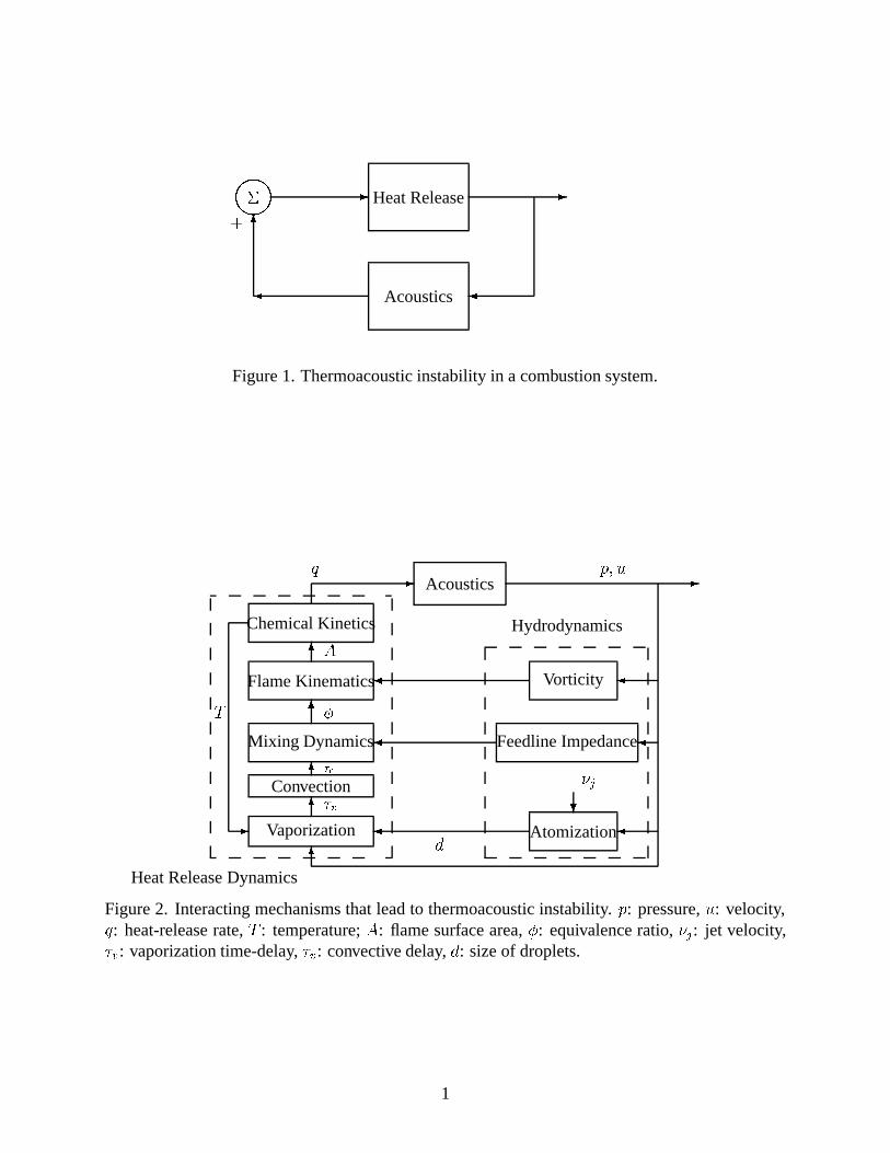
- Heat Release -

�Acoustics�

6�����

+

Figure 1. Thermoacoustic instability in a combustion system.

-q p; u

Acoustics -

d6

�Vorticity�Flame Kinematics

A6

Chemical Kinetics

�Feedline Impedance�Mixing Dynamics

�6

�c6

�?

�j

Atomization�Vaporization

6�vConvection

-

T

Heat Release Dynamics

Hydrodynamics

Figure 2. Interacting mechanisms that lead to thermoacoustic instability. p: pressure, u: velocity,q: heat-release rate, T : temperature; A: flame surface area, �: equivalence ratio, �j: jet velocity,�v: vaporization time-delay, �v: convective delay, d: size of droplets.

1

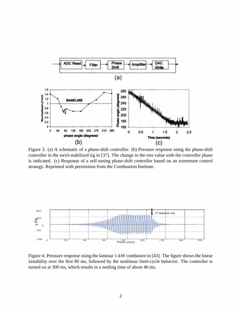
Figure 3. (a) A schematic of a phase-shift controller. (b) Pressure response using the phase-shiftcontroller in the swirl-stabilized rig in [37]. The change in the rms value with the controller phaseis indicated. (c) Response of a self-tuning phase-shift controller based on an extremum controlstrategy. Reprinted with permission from the Combustion Institute.

Figure 4. Pressure response using the laminar 1-kW combustor in [43]. The figure shows the linearinstability over the first 80 ms, followed by the nonlinear limit-cycle behavior. The controller isturned on at 300 ms, which results in a settling time of about 40 ms.

2

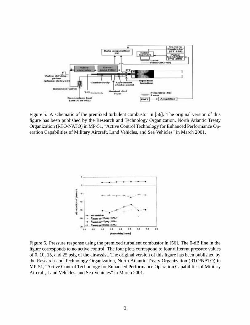
Figure 5. A schematic of the premixed turbulent combustor in [56]. The original version of thisfigure has been published by the Research and Technology Organization, North Atlantic TreatyOrganization (RTO/NATO) in MP-51, “Active Control Technology for Enhanced Performance Op-eration Capabilities of Military Aircraft, Land Vehicles, and Sea Vehicles” in March 2001.

Figure 6. Pressure response using the premixed turbulent combustor in [56]. The 0-dB line in thefigure corresponds to no active control. The four plots correspond to four different pressure valuesof 0, 10, 15, and 25 psig of the air-assist. The original version of this figure has been published bythe Research and Technology Organization, North Atlantic Treaty Organization (RTO/NATO) inMP-51, “Active Control Technology for Enhanced Performance Operation Capabilities of MilitaryAircraft, Land Vehicles, and Sea Vehicles” in March 2001.

3

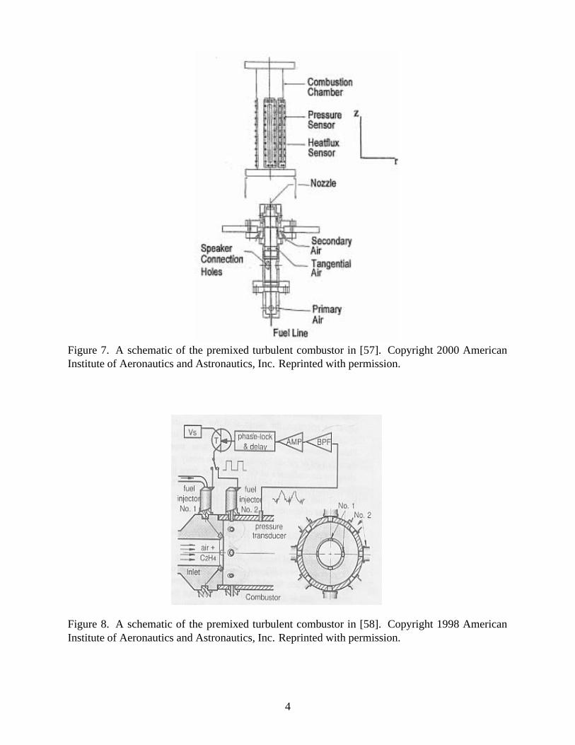
Figure 7. A schematic of the premixed turbulent combustor in [57]. Copyright 2000 AmericanInstitute of Aeronautics and Astronautics, Inc. Reprinted with permission.

Figure 8. A schematic of the premixed turbulent combustor in [58]. Copyright 1998 AmericanInstitute of Aeronautics and Astronautics, Inc. Reprinted with permission.

4

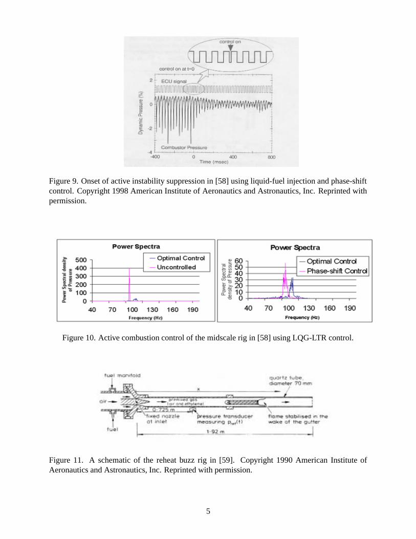
Figure 9. Onset of active instability suppression in [58] using liquid-fuel injection and phase-shiftcontrol. Copyright 1998 American Institute of Aeronautics and Astronautics, Inc. Reprinted withpermission.

Figure 10. Active combustion control of the midscale rig in [58] using LQG-LTR control.

Figure 11. A schematic of the reheat buzz rig in [59]. Copyright 1990 American Institute ofAeronautics and Astronautics, Inc. Reprinted with permission.

5

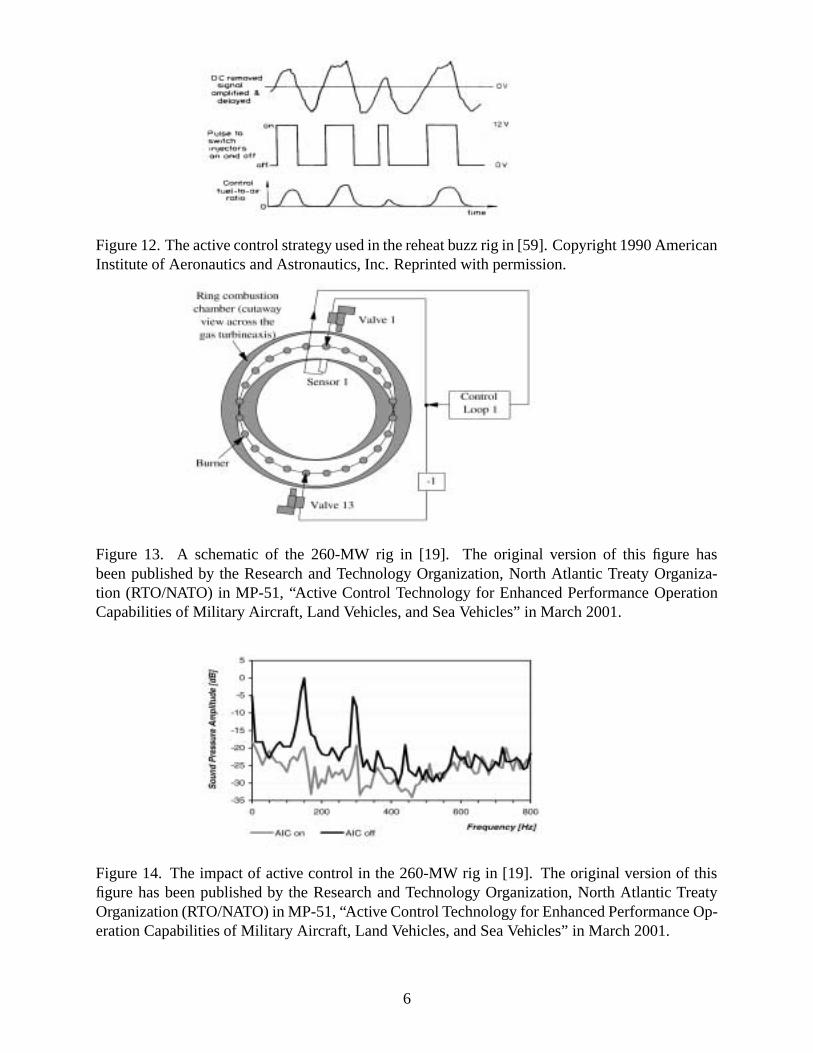
Figure 12. The active control strategy used in the reheat buzz rig in [59]. Copyright 1990 AmericanInstitute of Aeronautics and Astronautics, Inc. Reprinted with permission.

Figure 13. A schematic of the 260-MW rig in [19]. The original version of this figure hasbeen published by the Research and Technology Organization, North Atlantic Treaty Organiza-tion (RTO/NATO) in MP-51, “Active Control Technology for Enhanced Performance OperationCapabilities of Military Aircraft, Land Vehicles, and Sea Vehicles” in March 2001.

Figure 14. The impact of active control in the 260-MW rig in [19]. The original version of thisfigure has been published by the Research and Technology Organization, North Atlantic TreatyOrganization (RTO/NATO) in MP-51, “Active Control Technology for Enhanced Performance Op-eration Capabilities of Military Aircraft, Land Vehicles, and Sea Vehicles” in March 2001.

6