ACTEX(Please provide this information in case clarification is needed.) Send to: Stephen Camilli...
62
ACTEX Learning | Learn Today. Lead Tomorrow. ACTEX SOA Exam LTAM Study Manual Study Plus + gives you digital access* to: • Actuarial Exam & Career Strategy Guides • Technical Skill eLearning Tools • Samples of Supplemental Textbooks • And more! *See inside for keycode access and login instructions With Study Plus + Johnny Li, P.h.D., FSA | Andrew Ng, Ph.D., FSA Fall 2018 Edition | Volume I
Transcript of ACTEX(Please provide this information in case clarification is needed.) Send to: Stephen Camilli...

ACTEX Learning | Learn Today. Lead Tomorrow.
ACTEX SOA Exam LTAM Study Manual
StudyPlus+ gives you digital access* to:• Actuarial Exam & Career Strategy Guides
• Technical Skill eLearning Tools
• Samples of Supplemental Textbooks
• And more!
*See inside for keycode access and login instructions
With StudyPlus+
Johnny Li, P.h.D., FSA | Andrew Ng, Ph.D., FSA
Fall 2018 Edition | Volume I

ACTEX LearningNew Hartford, Connecticut
ACTEX SOA Exam LTAM Study Manual
Fall 2018 Edition
Johnny Li, P.h.D., FSA | Andrew Ng, Ph.D., FSA

Copyright © 2018 SRBooks, Inc.
ISBN: 978-1-63588-389-3
Printed in the United States of America.
No portion of this ACTEX Study Manual may bereproduced or transmitted in any part or by any means
without the permission of the publisher.
Actuarial & Financial Risk Resource Materials
Since 1972
Learn Today. Lead Tomorrow. ACTEX Learning

ACTEX LTAM Study Manual, Fall 2018 Edition
ACTEX is eager to provide you with helpful study material to assist you in gaining the necessary knowledge to become a successful actuary. In turn we would like your help in evaluating our manuals so we can help you meet that end. We invite you to provide us with a critique of this manual by sending this form to us at
your convenience. We appreciate your time and value your input.
Your opinion is important to us
Publication:
Very Good
A Professor
Good
School/Internship Program
Satisfactory
Employer
Unsatisfactory
Friend Facebook/Twitter
In preparing for my exam I found this manual: (Check one)
I found Actex by: (Check one)
I found the following helpful:
I found the following problems: (Please be specific as to area, i.e., section, specific item, and/or page number.)
To improve this manual I would:
Or visit our website at www.ActexMadRiver.com to complete the survey on-line. Click on the “Send Us Feedback” link to access the online version. You can also e-mail your comments to [email protected].
Name:Address:
Phone: E-mail:
(Please provide this information in case clarification is needed.)
Send to: Stephen Camilli ACTEX Learning
P.O. Box 715 New Hartford, CT 06057


NOT FOR PRINT: ADD KEYCODE TEMPLATE PAGE HERE

NOT FOR PRINT: ADD KEYCODE TEMPLATE PAGE HERE

Actex Learning | Johnny Li and Andrew Ng | SoA Exam LTAM
P-1 Preface
Contents
Preface P-7
Syllabus Reference P-10
Flow Chart P-13 Chapter 0 Some Factual Information C0-1
0.1 Traditional Life Insurance Contracts C0-1 0.2 Modern Life Insurance Contracts C0-3 0.3 Underwriting C0-3 0.4 Life Annuities C0-4 0.5 Pensions C0-6 Chapter 1 Survival Distributions C1-1
1.1 Age-at-death Random Variables C1-1 1.2 Future Lifetime Random Variable C1-4 1.3 Actuarial Notation C1-6 1.4 Curtate Future Lifetime Random Variable C1-10 1.5 Force of Mortality C1-12
Exercise 1 C1-20 Solutions to Exercise 1 C1-26 Chapter 2 Life Tables C2-1
2.1 Life Table Functions C2-1 2.2 Fractional Age Assumptions C2-6 2.3 Select-and-Ultimate Tables C2-17 2.4 Moments of Future Lifetime Random Variables C2-28 2.5 Useful Shortcuts C2-38
Exercise 2 C2-42 Solutions to Exercise 2 C2-51 Chapter 3 Life Insurances C3-1
3.1 Continuous Life Insurances C3-2 3.2 Discrete Life Insurances C3-17 3.3 mthly Life Insurances C3-26 3.4 Relating Different Policies C3-29 3.5 Recursions C3-36 3.6 Relating Continuous, Discrete and mthly Insurance C3-42 3.7 Useful Shortcuts C3-45
Exercise 3 C3-48 Solutions to Exercise 3 C3-61

Preface
Actex Learning | Johnny Li and Andrew Ng | SoA Exam LTAM
P-2
Chapter 4 Life Annuities C4-1
4.1 Continuous Life Annuities C4-1 4.2 Discrete Life Annuities (Due) C4-18 4.3 Discrete Life Annuities (Immediate) C4-25 4.4 mthly Life Annuities C4-29 4.5 Relating Different Policies C4-30 4.6 Recursions C4-34 4.7 Relating Continuous, Discrete and mthly Life Annuities C4-37 4.8 Useful Shortcuts C4-43
Exercise 4 C4-46 Solutions to Exercise 4 C4-60 Chapter 5 Premium Calculation C5-1
5.1 Traditional Insurance Policies C5-1 5.2 Net Premium and Equivalence Principle C5-3 5.3 Net Premiums for Special Policies C5-12 5.4 The Loss-at-issue Random Variable C5-18 5.5 Percentile Premium and Profit C5-27 5.6 The Portfolio Percentile Premium Principle C5-38
Exercise 5 C5-40 Solutions to Exercise 5 C5-63 Chapter 6 Net Premium Reserves C6-1
6.1 The Prospective Approach C6-2 6.2 The Recursive Approach: Basic Idea C6-15 6.3 The Recursive Approach: Further Applications C6-24
Exercise 6 C6-33 Solutions to Exercise 6 C6-50 Chapter 7 Insurance Models Including Expenses C7-1
7.1 Gross Premium C7-1 7.2 Gross Premium Reserve C7-5 7.3 Expense Reserve and Modified Reserve C7-13 7.4 Premium and Reserve Basis C7-23 7.5 Actual and Expected Profit C7-28
Exercise 7 C7-34 Solutions to Exercise 7 C7-52

Actex Learning | Johnny Li and Andrew Ng | SoA Exam LTAM
P-3 Preface
Chapter 8 Multiple Decrement Models: Theory C8-1
8.1 Multiple Decrement Table C8-1 8.2 Forces of Decrement C8-5 8.3 Associated Single Decrement C8-10 8.4 Discrete Jumps C8-22
Exercise 8 C8-29 Solutions to Exercise 8 C8-40 Chapter 9 Multiple Decrement Models: Applications C9-1
9.1 Calculating Actuarial Present Values of Cash Flows C9-1 9.2 Calculating Reserve C9-4 9.3 Calculating Profit C9-12
Exercise 9 C9-18 Solutions to Exercise 9 C9-26 Chapter 10 Multiple State Models C10-1
10.1 Discrete-time Markov Chain C10-4 10.2 Continuous-time Markov Chain C10-14 10.3 Kolmogorov’s Forward Equations C10-20 10.4 Calculating Actuarial Present Value of Cash Flows C10-34 10.5 Calculating Reserves C10-43
Exercise 10 C10-50 Solutions to Exercise 10 C10-67 Chapter 11 Multiple Life Functions C11-1
11.1 Multiple Life Statuses C11-2 11.2 Insurances and Annuities C11-17 11.3 Dependent Life Models C11-31
Exercise 11 C11-44 Solutions to Exercise 11 C11-64

Preface
Actex Learning | Johnny Li and Andrew Ng | SoA Exam LTAM
P-4
Chapter 12 Pension Plans and Retirement Benefits C12-1
12.1 The Salary Scale Function C12-1 12.2 Pension Plans C12-11 12.3 Setting the DC Contribution Rate C12-14 12.4 DB Plans and Service Table C12-18 12.5 Funding of DB Plans C12-38 12.6 Retiree Health Benefits C12-46
Exercise 12 C12-57 Solutions to Exercise 12 C12-73 Chapter 13 Profit Testing C13-1
13.1 Profit Vector and Profit Signature C13-1 13.2 Profit Measures C13-12 13.3 Using Profit Test to Compute Premiums and Reserves C13-16
Exercise 13 C13-24 Solutions to Exercise 13 C13-32 Chapter 14 Life Table Estimation C14-1
14.1 Complete and Grouped Data C14-1 14.2 The Kaplan-Meier Estimator C14-5 14.3 The Nelson-Aalen Estimator C14-12 14.4 Parametric Estimation of Death Probabilities C14-14 14.5 Calendar- and Anniversary-based Studies C14-18 14.6 Interval-based Study C14-23 14.7 Parametric Estimation of Q Matrix C14-25
Exercise 14 C14-27 Solutions to Exercise 14 C14-34 Chapter 15 Mortality Improvement Modeling C15-1
15.1 Some Facts and Jargons C15-1 15.2 Mortality Improvement Scales C15-4 15.3 Stochastic Mortality Models C15-15
Exercise 15 C15-30 Solutions to Exercise 15 C15-37
Actex Learning | Johnny Li and Andrew Ng | SoA Exam LTAM
P-5 Preface
Chapter 16 Health Benefits C16-1
16.1 Structured Settlements C16-1 16.2 Health Insurance Products C16-6 16.3 Modeling Health Insurance Products C16-16 16.4 Continuing Care Retiring Communities C16-21
Exercise 16 C16-25 Solutions to Exercise 16 C16-31 Appendix 1 Numerical Techniques A1-1
1.1 Numerical Integration A1-1 1.2 Euler’s Method A1-7 1.3 Solving Systems of ODEs with Euler’s Method A1-12 Appendix 2 Review of Probability A2-1
2.1 Probability Laws A2-1 2.2 Random Variables and Expectations A2-2 2.3 Special Univariate Probability Distributions A2-6 2.4 Joint Distribution A2-9 2.5 Conditional and Double Expectation A2-10 2.6 The Central Limit Theorem A2-12 Appendix 3 Illustrative Life Table A3-1

Preface
Actex Learning | Johnny Li and Andrew Ng | SoA Exam LTAM
P-6
Exam LTAM: General Information T0-1 Mock Test 1 T1-1
Solution T1-29 Mock Test 2 T2-1
Solution T2-28 Mock Test 3 T3-1
Solution T3-29 Mock Test 4 T4-1
Solution T4-30 Mock Test 5 T5-1
Solution T5-29 Mock Test 6 T6-1
Solution T6-29 Mock Test 7 T7-1
Solution T7-29 Mock Test 8 T8-1
Solution T8-29

Actex Learning | Johnny Li and Andrew Ng | SoA Exam LTAM
P-7 Preface
Suggested Solutions to MLC May 2012 S-1 Suggested Solutions to MLC Nov 2012 S-17 Suggested Solutions to MLC May 2013 S-29 Suggested Solutions to MLC Nov 2013 S-45 Suggested Solutions to MLC April 2014 S-55 Suggested Solutions to MLC Oct 2014 S-69 Suggested Solutions to MLC April 2015 S-81 Suggested Solutions to MLC Oct 2015 S-97 Suggested Solutions to MLC May 2016 S-109 Suggested Solutions to MLC Oct 2016 S-123 Suggested Solutions to MLC April 2017 S-133 Suggested Solutions to MLC Oct 2017 S-145 Suggested Solutions to MLC April 2018 S-157 Suggested Solutions to Sample Structural Questions S-169

Preface
Actex Learning | Johnny Li and Andrew Ng | SoA Exam LTAM
P-8
Preface
Thank you for choosing ACTEX. In 2018, the SoA launched Exam LTAM (Long-Term Actuarial Mathematics) to replace Exam MLC (Models for Life Contingencies). Compared to its predecessor, Exam LTAM has a much broader coverage. Topics that are newly introduced include the following: (1) Structural settlement and health insurance
You are required to know the calculations involved in structural settlements, which are often used in settling personal injury claims arising from motor vehicle accidents and medical malpractice. You also need to understand various types of health insurance, and know how to price them using complex multiple-state models.
(2) Mortality modeling
You are required to know several sophisticated mortality models, including the Lee-Carter model, the Cairns-Blake-Dowd model, the CBD M7 model, and MP-2014. You also need to know how to apply them in life insurance pricing and valuation.
(3) Retirement benefits
You are required to know how to value retiree health benefits. Although the set-up covered in Exam LTAM is a “simplified” one, the calculations are still quite involved.
(4) Estimation of life tables
You are required to know how life tables (and multiple state models) are estimated using advanced statistical methods. Previously, in Exam MLC, candidates were required to know how to apply them only.
In this brand new study manual, four chapters (Chapters 12, 14, 15 and 16; 216 pages in total) are written to cover these new (and very advanced) topics, ensuring you are best prepared for the exam! As a fact, one author (Professor Johnny Li) of this study manual has strong expertise in many of these exam topics. Professor Li published some 60 papers on mortality modeling and 2 books on personal injury claims. He also taught mortality modeling in a SoA live webcast. Some of his previous work has been adopted into the SoA’s study note (LTAM-21-18) for this exam. Exam LTAM has a very unique format. Among all preliminary exams, Exam LTAM is the only one that includes both multiple-choice and written-answer questions. We know very well that you may be worried about written-answer questions. To help you score the highest mark you can in the written-answer section, this manual contains more than 150 written-answer questions for you to practice. Eight full-length mock exams, written in exactly the same format as that announced in the SoA’s Exam LTAM Introductory Note, are also provided. Many of the written-answer questions in this study manual are highly challenging! We are sorry for giving you a hard time, but we do want you to succeed in the real exam.

Actex Learning | Johnny Li and Andrew Ng | SoA Exam LTAM
P-9 Preface
The learning outcomes stated in the syllabus of Exam LTAM require candidates to be able to interpret a lot of actuarial concepts. This skill is drilled extensively in our practice problems, which often ask you to interpret a certain actuarial formula or to explain your calculation. Also, in Exam LTAM you may be asked to define or describe a certain product, model or terminology. To help you prepare for this type of questions, Chapters 0 and 16 of this study manual provide you summaries of the definitions and descriptions of various products and terminologies. The summaries are written in a “fact sheet” style so that you can remember the key points more easily. Proofs and derivations are another key challenge. In Exam LTAM, you are highly likely to be asked to prove or derive something. You are expected to know, for example, how to derive the Kolmogorov forward differential equations for a certain transition probability. In this new study manual, we do teach (and drill) you how to prove or derive important formulas. This is in stark contrast to some other exam prep products in which proofs and derivations are downplayed, if not omitted. Besides the topics specified in the exam syllabus, you also need to know a range of numerical techniques, for example, Euler’s method and Simpson’s rule, in order to succeed. We know that you may not have even seen these techniques before, so we have prepared a special chapter (Appendix 1) to teach you all of the numerical techniques required for Exam LTAM. In addition, whenever a numerical technique is used, we clearly point out which technique it is, letting you follow our examples and exercises more easily. We have made our best effort to ensure that all topics in the syllabus are explained and practiced in sufficient depth. For your reference, a detailed mapping between this study manual and the readings in the exam syllabus is provided on pages P-11 to P-14. Other distinguishing features of this study manual include:
− All topics in the newest release (as of June 6, 2018) of LTAM-21-18 “Supplementary Note on Long Term Actuarial Mathematics” are fully incorporated into this study manual.
− We use graphics extensively. Graphical illustrations are probably the most effective way to explain formulas involved in Exam LTAM. The extensive use of graphics can also help you remember various concepts and equations.
− A sleek layout is used. The font size and spacing are chosen to let you feel more comfortable in reading. Important equations are displayed in eye-catching boxes.
− Rather than splitting the manual into tiny units, each of which tells you a couple of formulas only, we have carefully grouped the exam topics into 17 chapters and 3 appendices. Such a grouping allows you to more easily identify the linkages between different concepts, which are essential for your success as multiple learning outcomes can be examined in one single exam question.
− Instead of giving you a long list of formulas, we point out which formulas are the most important. Having read this study manual, you will be able to identify the formulas you must remember and the formulas that are just variants of the key ones.

Preface
Actex Learning | Johnny Li and Andrew Ng | SoA Exam LTAM
P-10
− We do not want to overwhelm you with verbose explanations. Whenever possible, concepts and techniques are demonstrated with examples and integrated into the practice problems.
− We explain multiple-state models in great depth. A solid understanding of multiple-state models is crucially important, because many of the learning objectives in Exam LTAM are related to multiple-state models.
− We teach you how to make tedious retiree health benefit calculations more manageable by using a tabular approach. Also, whenever possible, multiple methods (direct methods and computationally efficient algorithms) are presented.
− We write practice problems and mock exam questions in a similar format to the released exam questions. This arrangement helps you comprehend questions more quickly in the real exam.
− All mock exams in this study manual are based on the newest set of examination tables (the Standard Ultimate Life Table), so in the real exam, you can retrieve values from these tables more quickly.
On page P-15, you will find a flow chart showing how different chapters of this manual are connected to one another. You should first study Chapters 0 to 10 in order. Chapter 0 will give you some background factual information; Chapters 1 to 4 will build you a solid foundation; and Chapters 5 to 10 will get you to the core of the exam. You should then study Chapters 11 to 16 in any order you wish. Immediately after reading a chapter, do all practice problems we provide for that chapter. Make sure that you understand every single practice problem. Finally, work on the mock exams. Before you begin your study, please download the exam syllabus from the SoA’s website:
https://www.soa.org/Education/Exam-Req/edu-exam-ltam-detail.aspx
On the last page of the exam syllabus, you will find a link to Exam LTAM Tables, which are frequently used in the exam. You should keep a copy of the tables, as we are going to refer to them from time to time. You should also check the exam home page periodically for updates, corrections or notices. If you find a possible error in this manual, please let us know at the “Customer Feedback” link on the ACTEX homepage (www.actexmadriver.com). Any confirmed errata will be posted on the ACTEX website under the “Errata & Updates” link. Enjoy your study!

Actex Learning | Johnny Li and Andrew Ng | SoA Exam LTAM
P-11 Preface
Syllabus Reference
Our Manual AMLCR / SN Chapter 0: Some Factual Information
0.1 − 0.6 1
Chapter 1: Survival Distributions 1.1 2.1, 2.2 1.2 2.2 1.3 2.4 1.4 2.6 1.5 2.3
Chapter 2: Life Tables
2.1 3.1, 3.2 2.2 3.3 2.3 3.7, 3.8, 3.9 2.4 2.5, 2.6 2.5
Chapter 3: Life Insurances
3.1 4.4.1, 4.4.5, 4.4.7, 4.6 3.2 4.4.2, 4.4.6, 4.4.7, 4.6 3.3 4.4.3 3.4 4.4.8, 4.5 3.5 4.4.4 3.6 4.5 3.7
Chapter 4: Life Annuities
4.1 5.5 4.2 5.4.1, 5.4.2, 5.9, 5.10 4.3 5.4.3, 5.4.4 4.4 5.6 4.5 5.8 4.6 5.11.1 4.7 5.11.2, 5.11.3 4.8

Preface
Actex Learning | Johnny Li and Andrew Ng | SoA Exam LTAM
P-12
Our Manual AMLCR / SN Chapter 5: Premium Calculation
5.1 6.1, 6.2 5.2 6.5 5.3 6.5 5.4 6.4 5.5 6.7 5.6 6.8
Chapter 6: Net Premium Reserves
6.1 7.1, 7.3.1, 7.8 6.2 7.3.3 6.3 7.4
Chapter 7: Insurance Models Including Expenses
7.1 6.6 7.2 7.3.2, 7.5 7.3 7.9 7.4 6.7, 7.3.4 7.5 7.3.4
Chapter 8: Multiple Decrement Models: Theory
8.1 8.8 8.2 8.8, 8.9 8.3 8.8, 8.10 8.4 8.12
Chapter 9: Multiple Decrement Models: Applications
9.1 9.2 LTAM-21-18 Sec 3 9.3
Chapter 10: Multiple State Models
10.1 8.13, LTAM-21-18 Sec 3 10.2 8.2, 8.3, 8.11 10.3 8.4, 8.5 10.4 8.6 10.5 8.7, LTAM-21-18 Sec 3

Actex Learning | Johnny Li and Andrew Ng | SoA Exam LTAM
P-13 Preface
Our Manual AMLCR / SN Chapter 11: Multiple Life Functions
11.1 9.2 to 9.4 11.2 9.2 to 9.4 11.3 9.5 to 9.7
Chapter 12: Pension Plans and Retirement Benefits
12.1 10.3 12.2 10.1, 10.2 12.3 10.4 12.4 10.5, 10.6 12.5 10.5, 10.6 12.6 LTAM-21-18 Sec 6
Chapter 13: Profit Testing
13.1 12.2 to 12.4 13.2 12.5 13.3 12.6, 12.7
Chapter 14: Life Table Estimation
14.1 LTAM-22-18 12.1, 12.2 14.2 LTAM-22-18 12.3, 12.5 14.3 LTAM-22-18 12.3, 12.5 14.4 LTAM-22-18 12.8 14.5 LTAM-22-18 12.7 14.6 LTAM-22-18 12.7 14.7 LTAM-22-18 12.9

Preface
Actex Learning | Johnny Li and Andrew Ng | SoA Exam LTAM
P-14
Our Manual AMLCR / SN Chapter 15: Mortality Improvement Modeling
15.1 LTAM-21-18 Sec 4.1 15.2 LTAM-21-18 Sec 4.2 15.3 LTAM-21-18 Sec 4.3
Chapter 16: Health Benefits
16.1 LTAM-21-18 Sec 5 16.2 LTAM-21-18 Sec 1 (except 1.6) 16.3 LTAM-21-18 Sec 2 (except 2.4) 16.4 LTAM-21-18 Sec 1.6, 2.4
Appendix 1: Numerical Techniques
A1.1 8.6 A1.2 7.5.2 A1.3 7.5.2

Actex Learning | Johnny Li and Andrew Ng | SoA Exam LTAM
P-15 Preface
Flow Chart
1. Survival Distributions
2. Life Tables
3. Life Insurances
4. Life Annuities
6. Net Premium Reserves
8. Multiple Decrement Models: Theory
15. Mortality Improvement Modeling
10. Multiple State Models
11. Multiple Life Functions
A1. Numerical Techniques
5. Premium Calculation
7. Insurance Models Including Expenses
14. Life Table Estimation
0. Some Factual Information
13. Profit Testing
9. Multiple Decrement Models: Applications
12. Pension Plans and Retirement Benefits
16. Health Benefits
Preface
Actex Learning | Johnny Li and Andrew Ng | SoA Exam LTAM
P-16

This chapter serves as a summary of Chapter 1 in AMLCR. It contains descriptions of various life
insurance products and pension plans. There is absolutely no mathematics in this chapter.
You should know (and remember) the information presented in this chapter, because in the written
answer questions, you may be asked to define or describe a certain pension plan or life insurance
policy. Most of the materials in this chapter are presented in a “fact sheet” style so that you can
remember the key points more easily.
Many of the policies and plans mentioned in this chapter will be discussed in detail in later parts
of this study guide.
Whole life insurance
A whole life insurance pays a benefit on the death of the policyholder whenever it occurs. The
following diagram illustrates a whole life insurance sold to a person age x.
The amount of benefit is often referred to as the sum insured. The policyholder, of course, has to
pay the “price” of policy. In insurance context, the “price” of a policy is called the premium,
which may be payable at the beginning of the policy, or periodically throughout the life time of
the policy.
Time from now
0
(Age x)
A benefit (the
sum insured) is
paid here
Death occurs

Term life insurance
A term life insurance pays a benefit on the death of the policyholder, provided that death occurs
before the end of a specified term.
The time point n in the diagram is called the term or the maturity date of the policy.
Endowment insurance
An endowment insurance offers a benefit paid either on the death of the policyholder or at the end
of a specified term, whichever occurs earlier.
These three types of traditional life insurance will be discussed in Chapter 3 of this study guide.
Participating (with profit) insurance
Any premium collected from the policyholder will be invested, for example, in the bond market.
In a participating insurance, the profits earned on the invested premiums are shared with the
policyholder. The profit share can take different forms, for example, cash dividends, reduced
premiums or increased sum insured. You need not know the detail of this product.
Time from now
0 n
(Age x)
Death occurs here:
Pay a benefit Death occurs here:
Pay nothing
Time from now
0 n
(Age x)
Death occurs here:
Pay the sum
insured on death
Pay the sum
insured at time n if
the policyholder is
alive at time n

Modern life insurance products are usually more flexible and often involve an investment
component. The table below summarizes the features of several modern life insurance products.
Product Features
Universal life
insurance
Combines investment and life insurance
Premiums are flexible, as long as the accumulated value of the
premiums is enough to cover the cost of insurance
Unitized with-profit
insurance
Similar to traditional participating insurance
Premiums are used to purchase shares of an investment fund.
The income from the investment fund increases the sum insured.
Equity-linked
insurance
The benefit is linked to the performance of an investment fund.
Examples: equity-indexed annuities (EIA), unit-linked policies,
segregated fund policies, variable annuity contracts
Usually, investment guarantees are provided.
We will not discuss these policies in detail because it is out of the scope of this exam.
Underwriting refers to the process of collecting and evaluating information such as age, gender,
smoking habits, occupation and health history. The purposes of this process are:
To classify potential policyholders into broadly homogeneous risk categories
To determine if additional premium has to be charged.
The following table summarizes a typical categorization of potential policyholders.
Category
Characteristics
Preferred lives
Have very low mortality risk
Normal lives
Have some risk but no additional premium has to be charged
Rated lives
Have more risk and additional premium has to be charged
Uninsurable lives
Have too much risk and therefore not insurable
Underwriting is an important process, because with no (or insufficient) underwriting, there is a
risk of adverse selection; that is, the insurance products tend to attract high risk individuals,
leading to excessive claims. In Chapter 2, we will introduce the select-and-ultimate table, which
is closely related to underwriting.
A life annuity is a benefit in the form of a regular series of payments, conditional on the survival
of the policyholder. There are different types of life annuities.
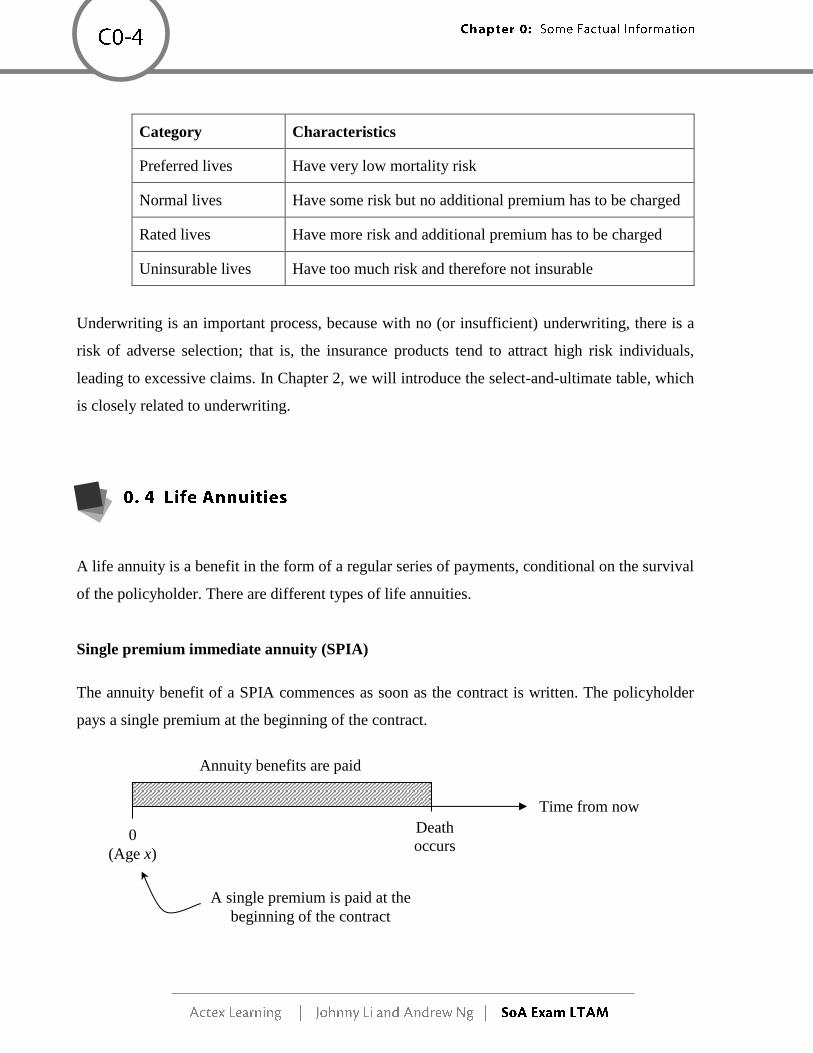
Single premium immediate annuity (SPIA)
The annuity benefit of a SPIA commences as soon as the contract is written. The policyholder
pays a single premium at the beginning of the contract.
Time from now
0
(Age x)
Death
occurs
Annuity benefits are paid
A single premium is paid at the
beginning of the contract

Single premium deferred annuity (SPDA)
The annuity benefit of a SPDA commences at some future specified date (say n years from now).
The policyholder pays a single premium at the beginning of the contract.
Regular Premium Deferred Annuity (RPDA)
An RPDA is identical to a SPDA except that the premiums are paid periodically over the deferred
period (i.e., before time n).
These three annuity types will be discussed in greater depth in Chapter 4 of this study guide.
Some life annuities are issued to two lives (a husband and wife). These life annuities can be
classified as follows.
Joint life annuity The annuity benefit ceases on the first death of the couple.
Last survivor annuity The annuity benefit ceases on the second death of the couple.
Reversionary annuity The annuity benefit begins on the first death of the couple, and
ceases on the second death.
These annuities will be discussed in detail in Chapter 11 of this study guide.
A single premium is paid at the
beginning of the contract
Time from now
0
(Age x)
n
The annuity benefit
begins at time n
Death
occurs

A pension provides a lump sum and/or annuity benefit upon an employee’s retirement. In the
following table, we summarize a typical classification of pension plans:
Defined contribution
(DC) plans
The retirement benefit from a DC plan depends on the accumulation
of the deposits made by the employ and employee over the employee’s
working life time.
Defined benefit (DB)
plans
The retirement benefit from a DB plan depends on the employee’s
service and salary.
Final salary plan: the benefit is a function of the employee’s
final salary.
Career average plan: the benefit is a function of the average salary
over the employee’s entire career in the
company.
Pension plans will be discussed in detail in Chapter 12 of this study guide.

Actex Learning | Johnny Li and Andrew Ng | SoA Exam LTAM
C1-1 Chapter 1: Survival Distributions
Chapter 1 Survival Distributions
1. To define future lifetime random variables 2. To specify survival functions for future lifetime random variables
3. To define actuarial symbols for death and survival probabilities and
develop relationships between them 4. To define the force of mortality
In Exam FM, you valued cash flows that are paid at some known future times. In Exam LTAM,
by contrast, you are going to value cash flows that are paid at some unknown future times.
Specifically, the timings of the cash flows are dependent on the future lifetime of the underlying
individual. These cash flows are called life contingent cash flows, and the study of these cash
flows is called life contingencies.
It is obvious that an important part of life contingencies is the modeling of future lifetimes. In this
chapter, we are going to study how we can model future lifetimes as random variables. A few
simple probability concepts you learnt in Exam P will be used.
Let us begin with the age-at-death random variable, which is denoted by T0. The definition of T0
can be easily seen from the diagram below.
1. 1 Age-at-death Random Variable

Chapter 1: Survival Distributions
Actex Learning | Johnny Li and Andrew Ng | SoA Exam LTAM
C1-2
The age-at-death random variable can take any value within [0, ). Sometimes, we assume that
no individual can live beyond a certain very high age. We call that age the limiting age, and denote
it by . If a limiting age is assumed, then T0 can only take a value within [0, ].
We regard T0 as a continuous random variable, because it can, in principle, take any value on the
interval [0, ) if there is no limiting age or [0, ] if a limiting age is assumed. Of course, to model
T0, we need a probability distribution. The following notation is used throughout this study guide
(and in the examination).
F0(t) Pr(T0 t) is the (cumulative) distribution function of T0.
f0(t) 0
d( )
dF t
t is the probability density function of T0. For a small interval t, the product
f0(t)t is the (approximate) probability that the age at death is in between t and t t.
In life contingencies, we often need to calculate the probability that an individual will survive to
a certain age. This motivates us to define the survival function:
S0(t) Pr(T0 t) 1 – F0(t).
Note that the subscript “0” indicates that these functions are specified for the age-at-death random
variable (or equivalently, the future lifetime of a person age 0 now).
Not all functions can be regarded as survival functions. A survival function must satisfy the
following requirements:
1. S0(0) 1. This means every individual can live at least 0 years.
2. S0() 0 or )(lim 0 tSt
0. This means that every individual must die eventually.
3. S0(t) is monotonically decreasing. This means that, for example, the probability of surviving
to age 80 cannot be greater than that of surviving to age 70.
T0 0
Age
Death occurs

Actex Learning | Johnny Li and Andrew Ng | SoA Exam LTAM
C1-3 Chapter 1: Survival Distributions
Summing up, f0(t), F0(t) and S0(t) are related to one another as follows.
Note that because T0 is a continuous random variable, Pr(T0 c) 0 for any constant c. Now, let
us consider the following example.
You are given that S0(t) 1 – t/100 for 0 t 100.
(a) Verify that S0(t) is a valid survival function.
(b) Find expressions for F0(t) and f0(t).
(c) Calculate the probability that T0 is greater than 30 and smaller than 60.
Solution
(a) First, we have S0(0) 1 – 0/100 1.
Second, we have S0(100) 1 – 100/100 0.
Third, the first derivative of S0(t) is 1/100, indicating that S0(t) is non-increasing.
Hence, S0(t) is a valid survival function.
(b) We have F0(t) 1 – S0(t) t/100, for 0 t 100.
Also, we have and f0(t) d
dtF0(t) 1/100, for 0 t 100.
(c) Pr(30 T0 60) S0(30) – S0(60) (1 – 30/100) – (1 – 60/100) 0.3.
F O R M U L A Relations between f0(t), F0(t) and S0(t)
, (1.1)
, (1.2)
Pr(a T0 b) = . (1.3)
Example 1.1 [Structural Question]
[ END ]
Chapter 1: Survival Distributions
Actex Learning | Johnny Li and Andrew Ng | SoA Exam LTAM
C1-4
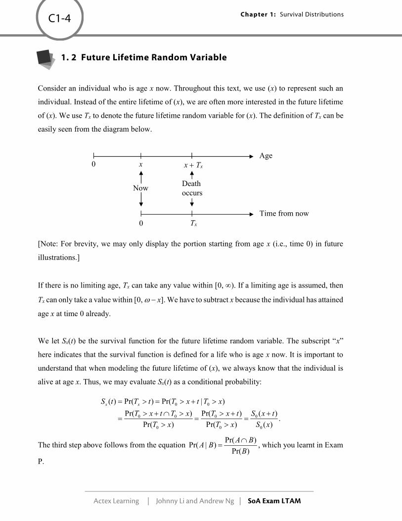
Consider an individual who is age x now. Throughout this text, we use (x) to represent such an
individual. Instead of the entire lifetime of (x), we are often more interested in the future lifetime
of (x). We use Tx to denote the future lifetime random variable for (x). The definition of Tx can be
easily seen from the diagram below.
[Note: For brevity, we may only display the portion starting from age x (i.e., time 0) in future
illustrations.]
If there is no limiting age, Tx can take any value within [0, ). If a limiting age is assumed, then
Tx can only take a value within [0, x]. We have to subtract x because the individual has attained
age x at time 0 already.
We let Sx(t) be the survival function for the future lifetime random variable. The subscript “x”
here indicates that the survival function is defined for a life who is age x now. It is important to
understand that when modeling the future lifetime of (x), we always know that the individual is
alive at age x. Thus, we may evaluate Sx(t) as a conditional probability:
0 0
0 0 0 0
0 0 0
( ) Pr( ) Pr( | )
Pr( ) Pr( ) ( ).
Pr( ) Pr( ) ( )
x xS t T t T x t T x
T x t T x T x t S x t
T x T x S x
The third step above follows from the equation Pr( )
Pr( | )Pr( )
A BA B
B
, which you learnt in Exam
P.
1. 2 Future Lifetime Random Variable
x Tx 0 Age
Time from now Tx 0
x
Death occurs
Now

Actex Learning | Johnny Li and Andrew Ng | SoA Exam LTAM
C1-5 Chapter 1: Survival Distributions
With Sx(t), we can obtain Fx(t) and fx(t) by using
Fx(t) 1 – Sx(t) and fx(t) d
( )d xF t
t,
respectively.
You are given that S0(t) 1 – t/100 for 0 t 100.
(a) Find expressions for S10(t), F10(t) and f10(t).
(b) Calculate the probability that an individual age 10 now can survive to age 25.
(c) Calculate the probability that an individual age 10 now will die within 15 years.
Solution
(a) In this part, we are asked to calculate functions for an individual age 10 now (i.e., x 10).
Here, 100 and therefore these functions are defined for 0 t 90 only.
First, we have 010
0
(10 ) 1 (10 ) /100( ) 1
(10) 1 10 /100 90
S t t tS t
S
, for 0 t 90.
Second, we have F10(t) 1 – S10(t) t/90, for 0 t 90.
Finally, we have 10 10
d 1( ) ( )
d 90f t F t
t .
(b) The probability that an individual age 10 now can survive to age 25 is given by
Pr(T10 15) S10(15) 1 90
15
6
5.
(c) The probability that an individual age 10 now will die within 15 years is given by
Pr(T10 15) F10(15) 1 S10(15) 6
1.
F O R M U L A
Survival Function for the Future Lifetime Random Variable
(1.4)
Example 1.2 [Structural Question]
[ END ]

Chapter 1: Survival Distributions
Actex Learning | Johnny Li and Andrew Ng | SoA Exam LTAM
C1-6
For convenience, we have designated actuarial notation for various types of death and survival
probabilities.
Notation 1: t px
We use t px to denote the probability that a life age x now survives to t years from now. By
definition, we have
t px Pr(Tx t) Sx(t).
When t 1, we can omit the subscript on the left-hand-side; that is, we write 1px as px.
Notation 2: t qx
We use t qx to denote the probability that a life age x now dies before attaining age x t. By
definition, we have
t qx Pr(Tx t) Fx(t).
When t 1, we can omit the subscript on the left-hand-side; that is, we write 1qx as qx.
Notation 3: t|u qx
We use t |u qx to denote the probability that a life age x now dies between ages x t and x t u.
By definition, we have
t|u qx Pr(t Tx t u) Fx(t u) Fx(t) Sx(t) Sx(t u).
When u 1, we can omit the subscript u; that is, we write t |1 qx as t | qx.
Note that when we describe survival distributions, “p” always means a survival probability, while
“q” always means a death probability. The “|” between t and u means that the death probability is
deferred by t years. We read “t | u” as “t deferred u”. It is important to remember the meanings of
these three actuarial symbols. Let us study the following example.
1. 3 Actuarial Notation

Actex Learning | Johnny Li and Andrew Ng | SoA Exam LTAM
C1-7 Chapter 1: Survival Distributions
Express the probabilities associated with the following events in actuarial notation.
(a) A new born infant dies no later than age 45.
(b) A person age 20 now survives to age 38.
(c) A person age 57 now survives to age 60 but dies before attaining age 65.
Assuming that S0(t) e0.0125t for t 0, evaluate the probabilities.
Solution
(a) The probability that a new born infant dies no later than age 45 can be expressed as 45q0. [Here
we have “q” for a death probability, x 0 and t 45.]
Further, 45q0 F0(45) 1 – S0(45) 0.4302.
(b) The probability that a person age 20 now survives to age 38 can be expressed as 18p20. [Here
we have “p” for a survival probability, x 20 and t 38 – 20 18.]
Further, we have 18p20 S20(18) 0
0
(38)
(20)
S
S 0.7985.
(c) The probability that a person age 57 now survives to age 60 but dies before attaining age 65
can be expressed as 3|5q57. [Here, we have “q” for a (deferred) death probability, x 57, t 60
– 57 3, and u 65 – 60 5.]
Further, we have 3|5q57 S57(3) – S57(8) 0
0
(60)
(57)
S
S 0
0
(65)
(57)
S
S = 0.058357.
[ END ]
Other than their meanings, you also need to know how these symbols are related to one another.
Here are four equations that you will find very useful.
Equation 1: t px t qx 1
This equation arises from the fact that there are only two possible outcomes: dying within t years
or surviving to t years from now.
Example 1.3

Chapter 1: Survival Distributions
Actex Learning | Johnny Li and Andrew Ng | SoA Exam LTAM
C1-8
Equation 2: t+u px t px u pxt
The meaning of this equation can be seen from the following diagram.
Mathematically, we can prove this equation as follows:
0 0 0
0 0 0
( ) ( ) ( )( ) ( ) ( )
( ) ( ) ( )t u x x x x t t x u x t
S x t u S x t S x t up S t u S t S u p p
S x S x S x t
.
Equation 3: t|u qx tu qx – t qx t px – tu px
This equation arises naturally from the definition of t|u qx.
We have t|u qx Pr(t Tx t u) Fx( t u) Fx( t ) t|u qx tu qx – t qx.
Also, t|u qx Pr(t Tx t u) Sx(t) Sx(t u) t px – tu px.
Equation 4: t|u qx t px u qxt
The reasoning behind this equation can be understood from the following diagram:
0 t t u
Time from now
Survive from time 0 to t: probability t px
Survive from time t to t u: probability u pxt
Survive from time 0 to t u: probability t+u px
(Age x) (Age x t)
Death occurs: prob.= uqxt Time from now
0 t t u
Survive from time 0 to time t: probability t px
t|u qx
(Age x) (Age x t)

Actex Learning | Johnny Li and Andrew Ng | SoA Exam LTAM
C1-9 Chapter 1: Survival Distributions
Mathematically, we can prove this equation as follows:
t|u qx t px – t u px (from Equation 3)
t px – t px u pxt (from Equation 2)
t px (1 u pxt )
t px u qxt (from Equation 1)
Here is a summary of the equations that we just introduced.
Let us go through the following example to see how these equations are applied.
You are given:
(i) px 0.99
(ii) px1 0.985
(iii) 3px1 0.95
(iv) qx3 0.02
Calculate the following:
(a) px3
(b) 2px
(c) 2px1
(d) 3px
(e) 1|2qx
F O R M U L A
Relations between t px, t qx and t|u qx
t px t qx 1, (1.5)
t+u px t px u pxt, (1.6)
t|u qx tu qx – t qx t px – tu px t px u qxt. (1.7)
Example 1.4

Chapter 1: Survival Distributions
Actex Learning | Johnny Li and Andrew Ng | SoA Exam LTAM
C1-10
Solution
(a) px3 1 – qx3
1 – 0.02 0.98
(b) 2px px px1
0.99 0.985 0.97515
(c) Consider 3px1 2px1 px3
0.95 2px1 0.98
2px1 0.9694
(d) 3px px 2px1
0.99 0.9694 0.9597
(e) 1|2qx px 2qx1
px (1 – 2px1)
0.99 (1 – 0.9694) 0.0303
[ END ]
In practice, actuaries use Excel extensively, so a discrete version of the future lifetime random
variable would be easier to work with. We define
x xK T ,
where y means the integral part of y. For example, 11 , 4.3 4 and 10.99 10. We
call Kx the curtate future lifetime random variable.
It is obvious that Kx is a discrete random variable, since it can only take non-negative integral
values (i.e., 0, 1, 2, …). The probability mass function for Kx can be derived as follows:
Pr(Kx 0) Pr(0 Tx 1) qx,
Pr(Kx 1) Pr(1 Tx 2) 1|1qx,
Pr(Kx 2) Pr(2 Tx 3) 2|1qx, …
1. 4 Curtate Future Lifetime Random Variable

Actex Learning | Johnny Li and Andrew Ng | SoA Exam LTAM
C1-11 Chapter 1: Survival Distributions
Inductively, we have
The cumulative distribution function can be derived as follows:
Pr(Kx k) Pr(Tx k 1) k1qx, for k 0, 1, 2, … .
It is just that simple! Now, let us study the following example, which is taken from a previous
SoA Exam.
For (x):
(i) K is the curtate future lifetime random variable.
(ii) qxk 0.1(k 1), k 0, 1, 2, …, 9
Calculate Var(K 3).
(A) 1.1 (B) 1.2 (C) 1.3 (D) 1.4 (E) 1.5
Solution
The notation means “minimum”. So here K 3 means min(K, 3). For convenience, we let W
min(K, 3). Our job is to calculate Var(W). Note that the only possible values that W can take are
0, 1, 2, and 3.
To accomplish our goal, we need the probability function of W, which is related to that of K. The
probability function of W is derived as follows:
Pr(W 0) Pr(K 0) qx 0.1
Pr(W 1) Pr(K 1) 1|qx
px qx1
F O R M U L A
Probability Mass Function for Kx
Pr(Kx k) k|1qx, k 0, 1, 2, … (1.8)
Example 1.5 [Course 3 Fall 2003 #28]

Chapter 1: Survival Distributions
Actex Learning | Johnny Li and Andrew Ng | SoA Exam LTAM
C1-12
(1 – qx)qx1
(1 – 0.1) 0.2 0.18
Pr(W 2) Pr(K 2) 2|qx
2px qx2 px px1 qx2
(1 – qx)(1 – qx1) qx2
0.9 0.8 0.3 0.216
Pr(W 3) Pr(K 3) 1 – Pr(K 0) – Pr(K 1) – Pr(K 2) 0.504.
From the probability function for W, we obtain E(W) and E(W 2
) as follows:
E(W) 0 0.1 1 0.18 2 0.216 3 0.5042.124
E(W 2 ) 02 0.1 12 0.18 22 0.216 32 0.5045.58
This gives Var(W) E(W 2
) – [E(W)]2 5.58 – 2.1242 1.07. Hence, the answer is (A).
[ END ]
In Exam FM, you learnt a concept called the force of interest, which measures the amount of
interest credited in a very small time interval. By using this concept, you valued, for example,
annuities that make payouts continuously. In this exam, you will encounter continuous life
contingent cash flows. To value such cash flows, you need a function that measures the probability
of death over a very small time interval. This function is called the force of mortality.
Consider an individual age x now. The force of mortality for this individual t years from now is
denoted by xt or x(t). At time t, the (approximate) probability that this individual dies within a
very small period of time t is xt t. The definition of xt can be seen from the following
diagram.
1. 5 Force of Mortality

Actex Learning | Johnny Li and Andrew Ng | SoA Exam LTAM
C1-13 Chapter 1: Survival Distributions
From the diagram, we can also tell that fx(t) t Sx(t)xtt. It follows that
fx(t) Sx(t)xt t pxxt .
This is an extremely important relation, which will be used throughout this study manual.
Recall that )()()( tStFtf xxx . This yields the following equation:
)(
)(
tS
tS
x
xtx
,
which allows us to find the force of mortality when the survival function is known.
Recall that d ln 1
d
x
x x , and that by chain rule,
)(
)(
d
)(lnd
xg
xg
x
xg for a real-valued function g. We
can rewrite the previous equation as follows:
)].(lnd[dd
)](lnd[
)(
)(
tStt
tS
tS
tS
xtx
xtx
x
xtx
Replacing t by u,
.dexp)(
)0(ln)(lnd
)](ln[dd
)](lnd[d
0
0
0
0
t
uxx
xx
t
ux
x
tt
ux
xux
utS
StSu
uSu
uSu
This allows us to find the survival function when the force of mortality is known.
Time from now
0 t t t
Survive from time 0 to time t: Prob. Sx(t)
Death occurs during t to t t:
Prob. xt t
Death between time t and t t: Prob. (measured at time 0) fx(t)t

Chapter 1: Survival Distributions
Actex Learning | Johnny Li and Andrew Ng | SoA Exam LTAM
C1-14
Not all functions can be used for the force of mortality. We require the force of mortality to satisfy
the following two criteria:
(i) xt 0 for all x 0 and t 0.
(ii)
0 duux .
Criterion (i) follows from the fact that xt t is a measure of probability, while Criterion (ii)
follows from the fact that )(lim tS xt
0.
Note that the subscript x t indicates the age at which death occurs. So you may use x to denote
the force of mortality at age x. For example, 20 refers to the force of mortality at age 20. The two
criteria above can then be written alternatively as follows:
(i) x 0 for all x 0.
(ii)
0 dxx .
The following two specifications of the force of mortality are often used in practice.
Gompertz’ law
x Bcx
Makeham’s law
x A Bcx
In the above, A, B and c are constants such that A B, B 0 and c 1.
F O R M U L A
Relations between xt, fx(t) and Sx(t)
fx(t) Sx(t)xt t pxxt, (1.9)
, (1.10)
(1.11)

Actex Learning | Johnny Li and Andrew Ng | SoA Exam LTAM
C1-15 Chapter 1: Survival Distributions
Let us study a few examples now.
For a life age x now, you are given that 2(10 )
( )100x
tS t
for 0 t 10.
(a) Find xt .
(b) Find fx(t).
Solution
(a) tt
t
tS
tS
x
xtx
10
2
100
)10(100
)10(2
)(
)(2
.
(b) You may work directly from Sx(t), but since we have found xt already, it would be quicker
to find fx(t) as follows:
fx(t) Sx(t)xt 2(10 ) 2 10
100 10 50
t t
t
.
[ END ]
For a life age x now, you are given
xt 0.002t, t 0.
(a) Is xt a valid function for the force of mortality of (x)?
(b) Find Sx(t).
(c) Find fx(t).
Solution
(a) First, it is obvious that xt 0 for all x and t.
Second, 2
00 0d 0.002 d 0.001x u u u u u
.
Hence, it is a valid function for the force of mortality of (x).
Example 1.6 [Structural Question]
Example 1.7 [Structural Question]

Chapter 1: Survival Distributions
Actex Learning | Johnny Li and Andrew Ng | SoA Exam LTAM
C1-16
(b) Sx(t) )001.0exp(d002.0expdexp 2
0
0 tuuu
tt
ux
.
(c) fx(t) Sx(t)xt 0.002texp(0.001t2).
[ END ]
You are given:
(i)
1
0 dexp1 tR tx
(ii)
1
0 d)(exp1 tkS tx
(iii) k is a constant such that S 0.75R.
Determine an expression for k.
(A) ln((1 – qx) / (1 0.75qx))
(B) ln((1 – 0.75qx) / (1 px))
(C) ln((1 – 0.75px) / (1 px))
(D) ln((1 – px) / (1 0.75qx))
(E) ln((1 – 0.75qx) / (1 qx))
Solution
First, R 1 – Sx(1) 1 px qx.
Second,
xk
xkt
txkt
tx peSeueukS
1)1(1dexp1d)(exp1
0
0 .
Since S 0.75R, we have
1 0.75
.1 0.75
kx x
k x
x
e p q
pe
q
Hence, 1
ln ln1 0.75 1 0.75
x x
x x
p qk
q q
and the answer is (A).
[ END ]
Example 1.8 [Course 3 Fall 2002 #35]

Actex Learning | Johnny Li and Andrew Ng | SoA Exam LTAM
C1-17 Chapter 1: Survival Distributions
(a) Show that when x Bcx, we have
)1( tx cc
xt gp ,
where g is a constant that you should identify.
(b) For a mortality table constructed using the above force of mortality, you are given that 10p50
0.861716 and 20p50 0.718743. Calculate the values of B and c.
Solution
(a) To prove the equation, we should make use of the relationship between the force of mortality
and tpx.
)1(ln
expdexpdexp00
txt sxt
sxxt ccc
BsBcsp .
This gives g exp(B/lnc).
(b) From (a), we have )1( 1050
861786.0 ccg and )1( 2050
718743.0 tccg . This gives
)861716.0ln(
)718743.0ln(
1
110
20
c
c.
Solving this equation, we obtain c = 1.02000. Substituting back, we obtain g 0.776856 and
B 0.00500.
[ END ]
Now, let us study a longer structural question that integrates different concepts in this chapter.
The function
18000
11018000 2xx
has been proposed for the survival function for a mortality model.
(a) State the implied limiting age .
(b) Verify that the function satisfies the conditions for the survival function S0(x).
Example 1.9 [Structural Question]
Example 1.10 [Structural Question]
Chapter 1: Survival Distributions
Actex Learning | Johnny Li and Andrew Ng | SoA Exam LTAM
C1-18
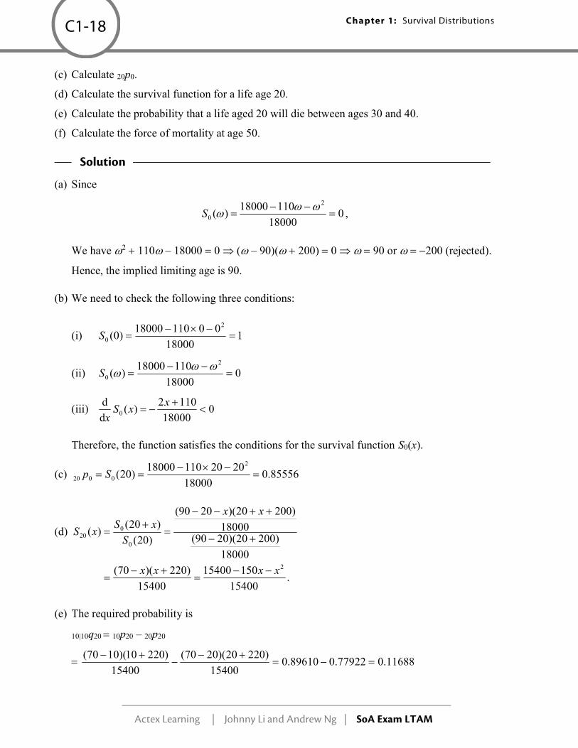
(c) Calculate 20p0.
(d) Calculate the survival function for a life age 20.
(e) Calculate the probability that a life aged 20 will die between ages 30 and 40.
(f) Calculate the force of mortality at age 50.
Solution
(a) Since
018000
11018000)(
2
0
S ,
We have 2 110 – 18000 0 ( – 90)( 200) 0 90 or 200 (rejected).
Hence, the implied limiting age is 90.
(b) We need to check the following three conditions:
(i) 118000
0011018000)0(
2
0
S
(ii) 018000
11018000)(
2
0
S
(iii) 018000
1102)(
d
d0
xxS
x
Therefore, the function satisfies the conditions for the survival function S0(x).
(c) 85556.018000
202011018000)20(
2
0020
Sp
(d)
.15400
15015400
15400
)220)(70(
18000
)20020)(2090(18000
)20020)(2090(
)20(
)20()(
2
0
020
xxxx
xx
S
xSxS
(e) The required probability is
10|10q20 10p20 – 20p20
11688.077922.089610.015400
)22020)(2070(
15400
)22010)(1070(
(d)

Actex Learning | Johnny Li and Andrew Ng | SoA Exam LTAM
C1-19 Chapter 1: Survival Distributions
(f) First, we find an expression for x.
)200)(90(
1102
18000
)200)(90(18000
2110
)(
)(
0
0
xx
xxx
x
xS
xSx .
Hence, 50 )20050)(5090(
110502
0.021.
[ END ]
You may be asked to prove some formulas in the structural questions of Exam LTAM. Please
study the following example, which involves several proofs.
Prove the following equations:
(a) xt ptd
d t pxx+t
(b) t
sxxsxt spq
0 d
(c) 1d
0
x
txxt tp
Solution
(a) LHS )(dd
d)dexp()dexp(
d
d
d
d
0
0
0 txxt
t
sx
t
sx
t
sxxt pst
sst
pt
RHS
(b) LHS t qx Pr(Tx t) spssft
sxxs
t
x dd)(
0
0 RHS
(c) LHS ttftpx
xtx
x
xt d)(d
0
0
xqx 1 RHS
[ END ]
Example 1.11 [Structural Question]

Chapter 1: Survival Distributions
Actex Learning | Johnny Li and Andrew Ng | SoA Exam LTAM
C1-20
1. [Structural Question] You are given:
0
1( )
1S t
t
, t 0.
(a) Find F0(t).
(b) Find f0(t).
(c) Find Sx(t).
(d) Calculate p20.
(e) Calculate 10|5q30. 2. You are given:
2
0
(30 )( )
9000
tf t
, for 0 t 30
Find an expression for t p5. 3. You are given:
0
20( )
200
tf t
, 0 t 20.
Find 10. 4. [Structural Question] You are given:
1
100x x
, 0 x 100.
(a) Find S20(t) for 0 t 80.
(b) Compute 40p20.
(c) Find f20(t) for 0 t 80. 5. You are given:
2
100x x
, for 0 x 100.
Find the probability that the age at death is in between 20 and 50. 6. You are given:
(i) S0(t)
t1 0 t , 0.
(ii) 40 220.
Find .
Exercise 1

Actex Learning | Johnny Li and Andrew Ng | SoA Exam LTAM
C1-21 Chapter 1: Survival Distributions
7. Express the probabilities associated with the following events in actuarial notation.
(a) A new born infant dies no later than age 35.
(b) A person age 10 now survives to age 25.
(c) A person age 40 now survives to age 50 but dies before attaining age 55.
Assuming that S0(t) e0.005t for t ≥ 0, evaluate the probabilities. 8. You are given:
2
0 ( ) 1100
tS t
, 0 t 100.
Find the probability that a person aged 20 will die between the ages of 50 and 60. 9. You are given:
(i) 2px 0.98
(ii) px2 0.985
(iii) 5qx0.0775
Calculate the following:
(a) 3px
(b) 2px3
(c) 2|3qx 10. You are given:
qxk 0.1(k 1), k 0, 1, 2, …, 9.
Calculate the following:
(a) Pr(Kx 1)
(b) Pr(Kx 2) 11. [Structural Question] You are given x for all x 0.
(a) Find an expression for Pr(Kx k), for k 0, 1, 2, …, in terms of and k.
(b) Find an expression for Pr(Kx k), for k 0, 1, 2, …, in terms of and k.
Suppose that 0.01.
(c) Find Pr(Kx 10).
(d) Find Pr(Kx 10).

Chapter 1: Survival Distributions
Actex Learning | Johnny Li and Andrew Ng | SoA Exam LTAM
C1-22
12. Which of the following is equivalent to
t
uxxu up
0 d ?
(A) t px
(B) t qx
(C) fx(t)
(D) – fx(t)
(E) fx(t)xt
13. Which of the following is equivalent to d
d t xpt
?
(A) –t px xt
(B) xt
(C) fx(t)
(D) –xt
(E) fx(t)xt 14. (2000 Nov #36) Given:
(i) x F e2x, x 0
(ii) 0.4p0 0.50
Calculate F.
(A) –0.20
(B) –0.09
(C) 0.00
(D) 0.09
(E) 0.20 15. (CAS 2004 Fall #7) Which of the following formulas could serve as a force of mortality?
(I) x Bcx, B 0, C 1
(II) x a(b x)1, a 0, b 0
(III) x (1 x)3, x 0
(A) (I) only
(B) (II) only
(C) (III) only
(D) (I) and (II) only
(E) (I) and (III) only

Actex Learning | Johnny Li and Andrew Ng | SoA Exam LTAM
C1-23 Chapter 1: Survival Distributions
16 (2002 Nov #1) You are given the survival function S0(t), where
(i) S0(t) 1, 0 t 1
(ii) S0(t)100
1te
, 1 t 4.5
(iii) S0(t) 0, 4.5 t
Calculate 4.
(A) 0.45
(B) 0.55
(C) 0.80
(D) 1.00
(E) 1.20
17. (CAS 2004 Fall #8) Given 1/ 2
0 ( ) 1100
tS t
, for 0 t 100, calculate the probability that
a life age 36 will die between ages 51 and 64. (A) Less than 0.15
(B) At least 0.15, but less than 0.20
(C) At least 0.20, but less than 0.25
(D) At least 0.25, but less than 0.30
(E) At least 0.30 18. (2007 May #1) You are given:
(i) 3p70 0.95
(ii) 2p71 0.96
(iii) 107.0d 75
71 xx
Calculate 5p70.
(A) 0.85
(B) 0.86
(C) 0.87
(D) 0.88
(E) 0.89

Chapter 1: Survival Distributions
Actex Learning | Johnny Li and Andrew Ng | SoA Exam LTAM
C1-24
19. (2005 May #33) You are given:
0.05 50 60
0.04 60 70x
x
x
Calculate 4|14q50 .
(A) 0.38
(B) 0.39
(C) 0.41
(D) 0.43
(E) 0.44 20. (2004 Nov #4) For a population which contains equal numbers of males and females at birth:
(i) For males, mx 0.10, x 0
(ii) For females, fx 0.08, x 0
Calculate q60 for this population. (A) 0.076
(B) 0.081
(C) 0.086
(D) 0.091
(E) 0.096 21. (2001 May #28) For a population of individuals, you are given:
(i) Each individual has a constant force of mortality.
(ii) The forces of mortality are uniformly distributed over the interval (0, 2).
Calculate the probability that an individual drawn at random from this population dies within one year. (A) 0.37
(B) 0.43
(C) 0.50
(D) 0.57
(E) 0.63
Actex Learning | Johnny Li and Andrew Ng | SoA Exam LTAM
C1-25 Chapter 1: Survival Distributions
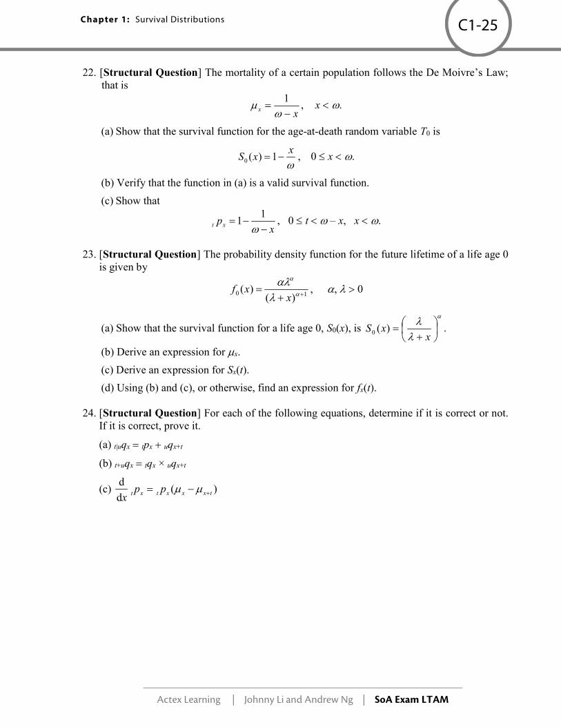
22. [Structural Question] The mortality of a certain population follows the De Moivre’s Law; that is
xx
1, x .
(a) Show that the survival function for the age-at-death random variable T0 is
x
xS 1)(0 , 0 x .
(b) Verify that the function in (a) is a valid survival function.
(c) Show that
xpxt
11 , 0 t – x, x .
23. [Structural Question] The probability density function for the future lifetime of a life age 0
is given by
10 )()(
xxf , , 0
(a) Show that the survival function for a life age 0, S0(x), is
xxS )(0 .
(b) Derive an expression for x.
(c) Derive an expression for Sx(t).
(d) Using (b) and (c), or otherwise, find an expression for fx(t). 24. [Structural Question] For each of the following equations, determine if it is correct or not.
If it is correct, prove it.
(a) t|uqx tpx uqxt
(b) tuqx tqx × uqxt
(c) )(d
dtxxxtxt pp
x

Chapter 1: Survival Distributions
Actex Learning | Johnny Li and Andrew Ng | SoA Exam LTAM
C1-26
Solutions to Exercise 1
1. (a) 0
1( ) 1
1 1
tF t
t t
.
(b) 0 0 2 2
d 1 1( ) ( )
d (1 ) (1 )
t tf t F t
t t t
.
(c) 0
0
1( ) 11( )
1( ) 11
x
S x t xx tS tS x x t
x
.
(d) p20 S20(1) 21/22.
(e) 10|5q30 10p30 – 15p30 S30(10) – S30(15) 1 30 1 30 31 31
1 30 10 1 30 15 41 46
0.0822.
2. S0(t)
27000
)30(
27000
)30(
9000
d)30(d)(
330330
230
0
tuuuuuf tt
t
.
If follows that 33
05 5 3
0
(5 ) (30 5 )( ) 1
(5) (30 5) 25t
S t t tp S t
S
.
3. S0(t)
400
)20(
400
)20(
200
d)20(d)(
220220
20
0
tuuuuuf tt
t
.
tt
t
tS
tft
20
2
400
)20(200
20
)(
)(2
0
0 .
Hence, 10 2/(20 – 10) 0.2.
4. (a) First, note that 20
1 1
100 20 80t t t
. We have
.80
1)80
80exp(ln))]80exp([ln(
d80
1expdexp)(
0
0
0 20200
ttu
uu
utS
t
tt
u
(b) 40p20 S20(40) 1 – 40/80 1/2.
(c) f20(t) S20(t)20t 1 1
180 80 80
t
t
.

Actex Learning | Johnny Li and Andrew Ng | SoA Exam LTAM
C1-27 Chapter 1: Survival Distributions
5. Our goal is to find Pr(20 T0 50) S0(20) – S0(50).
Given the force of mortality, we can find the survival function as follows:
2
0
0
0 0
1001)
100
100ln2exp())]100[ln(2exp(
d100
2expdexp)(
ttu
uu
utS
t
tt
u
So, the required probability is (1 – 20/100)2 – (1 – 50/100)2 0.82 – 0.52 0.39.
6. xx
x
xS
xSx
1
11
)(
)(
1
0
0 .
We are given that 40 220. This implies 2
40 20
, which gives 60.
7. (a) The probability that a new born infant dies no later than age 35 can be expressed as 35q0.
[Here we have “q” for a death probability, x 0 and t 35.]
Further, 35q0 F0(35) 1 – S0(35) 0.1605.
(b) The probability that a person age 10 now survives to age 25 can be expressed as 15p10. [Here we have “p” for a survival probability, x 10 and t 25 – 10 15.]
Further, we have 15p10 S10(15) )15(
)25(
0
0
S
S0.9277.
(c) The probability that a person age 40 now survives to age 50 but dies before attaining age 55 can be expressed as 10|5q40. [Here, we have “q” for a (deferred) death probability, x 40, t 50 – 40 10, and u 55 – 50 5.]
Further, we have 10|5q40 S40(10) – S40(15) 0
0
(50)
(40)
S
S 0
0
(55)
(40)
S
S = 0.0235.
8. The probability that a person aged 20 will die between the ages of 50 and 60 is given by
30|10q20 30p20 – 40p20 S20(30) – S20(40).
2
2
2
0
020 80
1
100
201
100
201
)20(
)20()(
t
t
S
tStS .
So, S20(30) 64
25
80
301
2
, S20(40)
64
16
80
401
2
. As a result, 30|10q20 9/64.

Chapter 1: Survival Distributions
Actex Learning | Johnny Li and Andrew Ng | SoA Exam LTAM
C1-28
9. (a) 3px 2px px2 0.98 0.985 0.9653.
3 2 3 5 5
52 3
3
1
1 1 0.07750.95566
0.9653
x x x x
xx
x
p p p q
qp
p
(c) 2|3qx 2px – 5px 0.98 – (1 – 0.0775) 0.0575. 10. (a) Pr(Kx 1) 1|qx px qx1 (1 – qx)qx1 (1 – 0.1) 0.2 0.18
(b) Pr(Kx 0) qx 0.1
Pr(Kx 2) 2|qx2px qx2 px px1 qx2 (1 – qx)(1 – qx1)qx2
0.9 0.8 0.3 0.216.
Hence, Pr(Kx 2) 0.1 0.18 0.216 0.496. 11. (a) Given that x for all x 0, we have t px et, px e and qx 1 – e.
Pr(Kx k) k|qx kpx qxk e k (1 – e).
(b) Pr(Kx k) k1qx 1 k1px 1 e(k 1).
(c) When 0.01, Pr(Kx 10) e10 0.01(1 – e0.01) 0.0090.
(d) When 0.01, Pr(Kx 10) 1 – e(10 + 1) 0.01 0.1042. 12. First of all, note that upx xu in the integral is simply fx(u).
)Pr(d)(d
0
0 tTuufup x
t
x
t
uxxu Fx(t) t qx.
Hence, the answer is (B).
13. Method I: We use t px = 1 t qx. Differentiating both sides with respect to t,
)()(d
d
d
d
d
dtftF
tq
tp
t xxxtxt .
Noting that fx(t) t px x+t, the answer is (A).
Method II: We differentiate t px with respect to t as follows:
.dd
ddexp
dexpd
d)(
d
d
d
d
0
0
0
t
ux
t
ux
t
uxxxt
ut
u
ut
tSt
pt
Recall the fundamental theorem of calculus, which says that )(d)(d
d
tguug
t
t
c . Thus
txxttx
t
uxxt pupt
)(dexp
d
d
0 .
Hence, the answer is (A).
(b)

Actex Learning | Johnny Li and Andrew Ng | SoA Exam LTAM
C1-29 Chapter 1: Survival Distributions
14. First, note that
0.4 0.4 20.4 0 0 0
0.5 exp d exp ( )duup u F e u .
The exponent in the above is 0.4
0.4 2 2
00
1( )d
2
0.4 1.11277 0.5
0.4 0.61277
u uF e u Fu e
F
F
As a result, 0.5 e0.4F0.61277, which gives F 0.2. Hence, the answer is (E). 15. Recall that we require the force of mortality to satisfy the following two criteria:
(i) x 0 for all x 0, (ii) 0
dx x
.
All three specifications of x satisfy Criterion (i). We need to check Criterion (ii).
We have
00
dln
xx Bc
Bc xc
,
00d ln( )
ax a b x
b x
,
and
3 200
1 1 1d
(1 ) 2(1 ) 2x
x x
.
Only the first two specifications can satisfy Criterion (ii). Hence, the answer is (D).
[Note: x Bcx is actually the Gompertz’ law. If you knew that you could have identified that x Bcx can serve as a force of mortality without doing the integration.]
16. Recall that )(
)(
tS
tS
x
xtx
.
Since we need 4, we use the definition of S0(t) for 1 t 4.5:
0 ( ) 1100
teS t ,
100)(0
tetS .
As a result,
4
4
4 4 4100 1.203
1001
100
ee
e e
. Hence, the answer is (E).

Chapter 1: Survival Distributions
Actex Learning | Johnny Li and Andrew Ng | SoA Exam LTAM
C1-30
17. The probability that a life age 36 will die between ages 51 and 64 is given by
S36(15) – S36(28).
We have 8
64
64
64
100
361
100
361
)36(
)36()(
2/1
2/1
2/1
0
036
tt
t
S
tStS
.
This gives S36(15)8
7 and S36(28)
8
6 . As a result, the required probability is
S36(15) – S36(28) 1/8 0.125. Hence, the answer is (A). 18. The computation of 5p70 involves three steps.
First, 3 7070
2 71
0.950.9896
0.96
pp
p .
Second, 75
71 d 0.107
4 71 0.8985x x
p e e .
Finally, 5p70 0.9896 0.8985 0.889. Hence, the answer is (E). 19. 4p50 e0.05 4 0.8187
10p50 e0.05 10 0.6065
8p60 e0.04 8 0.7261
18p50 10p50 8p60 0.6065 0.7261 0.4404
Finally, 4|14q50 4p50 – 18p50 0.8187 – 0.4404 0.3783. Hence, the answer is (A). 20. For males, we have
0 0d 0.10d 0.10
0 ( )t tm
u u um tS t e e e .
For females, we have
0 0d 0.08d 0.08
0 ( )t tf
u u uf tS t e e e .
For the overall population,
0.1 60 0.08 60
0 (60) 0.0053542
e eS
,
and
0.1 61 0.08 61
0 (61) 0.004922
e eS
.

Actex Learning | Johnny Li and Andrew Ng | SoA Exam LTAM
C1-31 Chapter 1: Survival Distributions
Finally, 060 60
0
(61)1 1 0.081
(60)
Sq p
S . Hence, the answer is (B).
21. Let M be the force of mortality of an individual drawn at random, and T be the future lifetime
of the individual. We are given that M is uniformly distributed over (0, 2). So the density function for M is fM() 1/2 for 0 2 and 0 otherwise.
This gives
0
2
0
2
2
Pr( 1)
E[Pr( 1| )]
Pr( 1| ) ( )d
1(1 ) d
21
(2 1)21
(1 )20.56767.
M
T
T M
T M f
e
e
e
Hence, the answer is (D). 22. (a) We have, for 0 x ,
x
esss
sxSx
xxx
s
1)]exp([ln()d1
exp()dexp()()1ln(
0
0
0 0 .
(b) We need to check the following three conditions:
(i) S0(0) 1 – 0/ 1
(ii) S0() 1 – / 0
(iii) S 0() 1/ 0 for all 0 ≤ x < , which implies S0(x) is non-increasing.
Hence, the function in (a) is a valid survival function.
(c) x
t
x
txx
tx
xS
txSpxt
11
1
)(
)(
0
0 , for 0 t – x, x .
23. (a)
x x
xs
sssfxFxS
0 0 1000 )(d
)(1d)(1)(1)(
.
(b) xxS
xfx
)(
)(
0
0 .

Chapter 1: Survival Distributions
Actex Learning | Johnny Li and Andrew Ng | SoA Exam LTAM
C1-32
(c) .)(
)()(
0
0
tx
x
x
txxS
txStS x
(d) txtx
xtStf txxx
)()( .
24. (a) No, the equation is not correct. The correct equation should be t|uqx tpx × uqxt. (b) No, the equation is not correct. The correct equation should be tupx tpx × upxt. (c) Yes, the equation is correct. The proof is as follows:
)(
)(
)(
)(
)(
)(
)(
)(
)(
)(
)(
)(
)(
)(
)(
)]([
))())(())()((
)]([
)(')()(')(
)(
)(
d
d
d
d
0
0
0
0
0
0
0
0
0
0
0
0
0
0
20
0000
20
0000
0
0
txxxt
xxtxttx
xt
p
pp
xS
xf
xS
txS
xS
txS
txS
txf
xS
xf
xS
txS
xS
txf
xS
xftxStxfxS
xS
xStxStxSxS
xS
txS
xp
x