Page 1/20

Cross-scale evaluation of catchment- and global-scalehydrological model simulations of drought characteristicsacross eight large river catchmentsAmit Kumar  ( amit1792kumar@gmail.com )

University of Nottingham https://orcid.org/0000-0001-6444-4047Simon N Gosling 

University of NottinghamMatthew F Johnson 

University of NottinghamJamal Zaherpour 

University of NottinghamGuoyong Leng 

Key Laboratory of Water Cycle & Related Land Surface Processes Chinese Academy of SciencesHannes Muller Schmied 

Goethe University FrankfurtJenny Kupzig 

Ruhr-Universitat BochumLutz Breuer 

Justus Liebig Universitat GiessenNaota Hanasaki 

National Institute for Environmental Studies, TsukubaQiuhong Tang 

Key Laboratory of Water Cycle & Related Land Surface Processes Chinese Academy of SciencesRohini Kumar 

Helmholtz Centre for Environmental Research - UFZSebastian Ostberg 

Potsdam Institute for Climate Impact ResearchTobias Stacke 

Helmholtz-Zentrum GeesthachtYadu Pokhrel 

Michigan State University Department of Civil and Environmental EngineeringYoshihide Wada 

Utrecht University: Universiteit UtrechtYoshimitsu Masaki 

Ibaraki University

Research Article

Keywords: catchment scale hydrological models, global scale hydrological models, drought

Page 2/20

Posted Date: April 26th, 2021

DOI: https://doi.org/10.21203/rs.3.rs-409757/v1

License: This work is licensed under a Creative Commons Attribution 4.0 International License.   Read Full License

Page 3/20

AbstractAlthough global- and catchment-scale hydrological models are often shown to accurately simulate long-term runoff time-series, far less is known about their suitability for capturing hydrological extremes, such as droughts. Here we evaluatedrunoff simulations from nine catchment scale hydrological models (CHMs) and eight global scale hydrological models(GHMs) for eight large catchments: Upper Amazon, Lena, Upper Mississippi, Upper Niger, Rhine, Tagus, Upper Yangtze andUpper Yellow. The simulations were conducted within the framework of phase 2a of the Inter-Sectoral Impact ModelIntercomparison Project (ISIMIP2a). We evaluated the ability of the CHMs, GHMs and their respective ensemble means(Ens-CHM and Ens-GHM) to simulate observed monthly runoff and hydrological droughts over 31 years (1971–2001).Observed and simulated hydrological drought events were identi�ed using the Standardised Runoff Index (SRI) and wereclassi�ed based on intensity. Our results show that for all eight catchments, CHMs out-performed GHMs in monthly runoffestimation showing a better representation of observed runoff than GHMs. The number of drought events identi�ed underdifferent drought categories (i.e. SRI values of -1 to -1.49, -1.5 to -1.99, and ≤-2) varied signi�cantly between models. Allthe models, as well as the two ensemble means present limited ability to accurately simulate severe drought events in alleight catchments, in terms of their timing and intensity. By analysing the monthly runoff time-series for several extremedroughts over the historical period, we identify room for improvement in the models so that extreme droughts mayultimately be better represented by both CHMs and GHMs.

1. IntroductionA drought is an event where water availability is lower than normal, resulting in a failure to ful�l the water demands ofdifferent natural systems and socioeconomic sectors (WMO 1986). From 1991 to 2005, 950 million people were affectedby droughts worldwide and economic damage of 100 billion US dollars was reported (UN and UNISDR, UNDP 2009).Droughts are usually the consequence of a prolonged period of below normal precipitation that also affects many otherenvironmental, climate and social variables (Lloyd-Hughes 2014; Van Loon 2015). As a result, drought events can bedi�cult to identify in space and time, which makes it one of the most complex natural hazards (Wilhite 1993; Wilhite,Hayes and Svoboda 2000). Researchers, managers and policy makers quantify drought events using drought indicesbased on climate data (reviewed in Heim 2002; Keyantash and Dracup 2002; Mishra and Singh 2010). Whilst precipitationis a key input in calculating these indices, other climate and environmental variables that affect water storage andavailability, are also signi�cant.

Droughts are complex natural disasters as their onset and magnitude is related to the interaction between manyhydrological and climatological processes. Droughts can be classi�ed into different types namely meteorological,hydrological, agricultural and socioeconomic droughts. Meteorological droughts represent below normal precipitation andare mainly presented by precipitation driven indices such as the Standardised Precipitation Index (SPI; McKee, Doeskenand Kliest 1993), Regional Drought Area Index (RDAI; Fleig et al. 2011) and Effective drought index (EDI; Byun and Wilhite1999). In contrast, hydrological droughts de�ne effects on freshwater storage, which are represented by indices that usestream �ows, reservoir levels, groundwater levels or other similar variables. Hydrological droughts are often closely relatedto meteorological droughts and can also be exacerbated by environmental changes, anthropogenic activities, andmismanagement of water resources (Tallaksen et al. 2004).

Studies on hydrological droughts at global or continental scales increasingly use Land Surface Models (LSMs), GlobalHydrological Models (GHMs) and Catchment Scale Hydrological Models (CHMs) to quantify and predict drought events(Gosling, Zaherpour, et al. 2017; Hattermann et al. 2017). GHMs, LSMs and CHMs have been widely used to model �oodhazards and risk (Arnell and Gosling 2016), climate change mitigation (Irvine et al. 2017), forecasting at shorter timescales (Emerton et al. 2016) and food security (Elliott et al. 2014). The use of these models to study droughts is alsorelatively common (Van Huijgevoort et al. 2013; Prudhomme et al. 2014) but there is relatively less information on theperformance of the models for simulating drought. Given the societal signi�cance of drought prediction under climate

Page 4/20

change scenarios (Pokhrel et al. 2021) using these tools, and the in�uence of results on climate change adaptation andmitigation decision-making, it is critical to understand their strengths and limitations when speci�cally focusing ondrought conditions.

Model inter-comparison projects like WaterMIP (Haddeland et al. 2011) and the Inter-Sectoral Impact Model Inter-comparison Project (ISIMIP) (Frieler et al. 2017) have made it possible to evaluate and compare simulations for historicaland future periods from ensembles of GHMs and CHMs driven by common input datasets. Although recent studies haveexploited these two MIPs to evaluate the general performance of ensembles of GHMs (Haddeland et al. 2011; Prudhommeet al. 2014; Zaherpour et al. 2018), CHMs (Dams et al. 2015; Huang et al. 2017), or both GHMs and CHMs together(Hattermann et al. 2017; Krysanova et al. 2020), none have comprehensively evaluated the relative capabilities of twolarge-scale multi-model ensembles of GHMs and CHMs to represent historical hydrological drought.

This study provides a �rst insight into the relative abilities of GHMs and CHMs to simulate hydrological drought events(hereafter referred to as ‘droughts’). We used GHM and CHM simulations from ISIMIP2a (Gosling, Müller Schmied, et al.2017) to identify historical drought events from their respective monthly runoff simulations, and evaluated how thesedroughts compared to the observed record. The main objectives of this study were, �rstly, to systematically evaluate theperformance of global scale and catchment scale hydrological models to simulate droughts and, secondly, to analyse thesimulated drought by ensemble mean to determine how well it represents droughts simulated by individual models.Finally, we discuss the opportunities for improving the simulation of drought events by both GHMs and CHMs.

2. Data And Methods

2.1. Study CatchmentsEight large (> 65,000 km2) catchments were selected to cover important climate zones and hydrological systems aroundthe globe. These were, the Upper Amazon, Lena, Upper Mississippi, Upper Niger, Rhine, Tagus, Upper Yangtze and UpperYellow (Fig. 1). They are the same eight catchments used in previous ‘cross-scale’ GHM-CHM comparisons (Gosling,Zaherpour, et al. 2017; Hattermann et al. 2017). For the analysis, only the upper part of the Amazon, Mississippi, Niger,Yangtze and Yellow were modelled due to their complicated geomorphological structure and human alterations furtherdownstream (Krysanova and Hattermann 2017). Catchment boundaries were de�ned according to Drainage DirectionMaps at 30′ (DDM30; Döll and Lehner 2002) for the GHMs and CHMs, and according to the Global Runoff Data Centre(GRDC; http://grdc.bafg.de) for the observed data.

2.2. Models and input dataSimulated runoff data from eight GHMs and nine CHMs along with corresponding observed runoff data from the GRDC,for 1971–2001, were used in this study. Observed runoff data was acquired from the most downstream gauge in theGRDC catalogue for each catchment. All GHMs and CHMs were run with input climate data from WATCH ERA-40 (Weedonet al. 2011) for the period 1971–2001. Output from the models is openly available from the Earth System Grid Federation(ESGF; https://esg.pik-potsdam.de/search/isimip) for the GHMs (Gosling, Müller Schmied, et al. 2017) and the CHMs(Krysanova et al. 2017). All the GHMs provided outputs for all catchments; however, the number of CHMs with simulatedrunoff varied by catchment (Table 1). Following the method described by Haddeland et al. (2011), monthly observed andsimulated runoff data was converted to catchment-mean monthly runoff by using the area upstream of the gaugeaccording to the DDM30 river network. Thus, an area correction factor was applied to the GRDC runoff data to account forthe fact that the river network, which is at 0.5° spatial resolution, may not perfectly overlap with the GRDC river catchmentboundaries (Table 1).

Both GHMs and CHMs simulate the full hydrological cycle with predominantly daily precipitation and temperature as inputdata. All the GHMs simulated hydrological processes at a spatial resolution of 0.5° x 0.5° across the global land surface.

Page 5/20

In contrast, CHMs operated using various approaches; three CHMs run on a grid (mHM, VIC, WaterGAP3), four by splittingthe catchment into sub-catchments and smaller hydrological response units (HBV, HYPE, SWAT, SWIM) and one byconsidering the whole catchment as a single entity (HYMOD). The GHMs were not calibrated to catchment speci�cconditions, except WaterGAP2 (which was calibrated against long-term average monthly runoff for a number of gaugesworldwide) while the CHMs were calibrated and the performance of the calibration evaluated in a separate validationperiod using the WATCH reanalysis climate forcing data (Huang et al. 2017).

In addition to the individual model results, we calculated the corresponding ensemble mean for the GHMs and CHMsrespectively for every catchment and included them in the analysis, for meeting our second study objective. For thepurposes of this study, all the models were treated as independent even though many of the models operate on similarmodel parameterisation. No hydrological model was excluded or weighted based on their performance on simulatingpresent day runoff.

2.3. Drought Indicator and performance evaluationSeveral standardised indices have been developed for identifying hydrological droughts, such as the Palmer HydrologicalDrought Index(PDSI; Jacobi et al. 2013), Water Supply Index (WSI; Garen 1993) and Standardised Stream�ow/RunoffIndex (SSI/SRI; Vicente-Serrano et al. 2012). In comparison with PHDI and WSI, SSI is more commonly accepted due thefact that it is simple to calculate, can be used on various time scales and above all, requires fewer inputs. SSI isextensively used in many studies (Shukla and Wood 2008; Vicente-Serrano et al., 2012; Wu et al. 2018; Liu et al. 2019).Calculation of SSI/SRI is similar to that of Standardised Precipitation Index (SPI) proposed by McKee, Doesken and Kliest(1993) but considering runoff instead of precipitation. The SRI values are determined based on long-term runoff records(preferably > 30 years) by aggregating the monthly runoff over an accumulation period (1, 3, 6, 12, or 24 months). The newseries formed after accumulation (1 month for this study) is then �tted to a probability distribution that subsequently istransformed to a normal distribution such that the mean SRI is zero. The “SPEI” package in R (Beguería and Vicente-Serrano 2017) was used for all the calculations of SRI. “SPEI” i.e. Standardized Precipitation-Evapotranspiration Indexpackage facilitates computation of SPI and other variants of SPI (SRI for our study) by providing de�ned functions thatcan be used directly in the R working environment. Any positive SRI values indicate runoff values greater than the meanmonthly runoff and vice versa. Any SRI value less than − 1 was considered to indicate drought condition. These droughtconditions were categorised based on SRI values into three drought categories namely moderate, severe and extremedroughts. SRI values from − 1 to -1.49 signi�es moderate drought, from − 1.5 to -1.99 severe drought, and all the SRIvalues less than − 2 as extreme drought.

Continuous SRI values -1 signi�ed drought events, which lasted until the SRI rose above − 1 again. Two main factors playan important role in the identi�cation a drought event: the intensity and duration. Therefore, all the comparisons madebetween observed and modelled records were based on intensity, duration and frequency of drought events. We calculatedthree drought characteristics – drought intensity, drought duration and frequency of drought events to analysehydrological drought conditions for all eight catchments. Run theory method (Yevjevich and Ica Yevjevich 1967) was usedfor the extraction of drought characteristics from drought index series i.e. SRI time series. The drought duration (inmonths) was taken as the period the SRI remained -1, and the minimum SRI value in this period was used as the droughtintensity.

We used the coe�cient of determination i.e. the square of Pearson product moment correlation coe�cient (R2) with acon�dence interval of 0.95, and the Nash-Sutcliffe coe�cient (NSE; Nash and Sutcliffe 1970) to evaluate the goodness of�t between observed runoff and simulated runoff obtained from different CHMs and GHMs. R2 indicated the strength ofrelationship between the simulated and observed runoff, and NSE indicated the models e�ciency (range - to 1). NSEvalues approaching 1 indicate a perfect match of simulated and observed runoff values while negative values show thatthe observed mean is a better predictor than the model.

Page 6/20

3. Results

3.1. Comparison of observed and simulated runoffBoth the R2 and NSE were used for capturing nuances between simulated and observed runoff. Table 2 shows the R2 andNSE values between observed monthly runoff and all the CHMs and GHMs incorporated in the analysis, including theensemble mean of the GHMs (Ens-GHM) and CHMs (Ens-CHM) respectively. All the direct comparisons drawn betweenCHMs and GHMs are based upon Ens-CHM and Ens-GHM, and not the individual CHMs or GHMs.

For all eight catchments, CHMs out-performed GHMs in runoff estimation showing a better representation of observedrunoff than GHMs. Ens-CHM and Ens-GHM have R2 values greater than 0.7 (Moriasi et al. 2007, 2015) for all catchmentsexcept for Lena by Ens-GHM. Comparing both ensemble outputs, R2 values of Ens-CHM were higher than those of Ens-GHM for all catchments. Similarly, NSE values of Ens-CHM for all eight catchments were greater than 0.7 and closer to 1for Rhine, Tagus and Yangtze catchments, while for Ens-GHM only two catchments i.e. Yangtze and Yellow had NSEvalues greater than 0.7, with negative values for the Niger and Rhine.

3.2. Comparison of observed and simulated SRIR2 and NSE values for SRI series obtained from simulated runoff outputs from CHMs and GHMs are shown in Table 3,including the ensembles i.e. Ens-GHM and Ens-CHM. Both R2 and NSE vary widely across all catchments for both GHMsand CHMs. The R2 values of the ensemble series varied between 0.18 (Ens-GHM) and 0.94 (Ens-CHM) while the NSEranged from − 0.14 (Ens-GHM) to 0.95 (Ens-CHM) across all catchments. The catchments where most of the models (bothGHMs and CHMs) performed well were the Mississippi and Rhine, both with R2 and NSE values for Ens-CHM and Ens-GHM > 0.85. For both these catchments, individual models always had R2 > 0.50 and NSE values > 0.40. No individualGHM or CHM achieved R2 and NSE values > 0.7 for the other six catchments, with the exception of HBV for the Taguscatchment (R2 = 0.75 and NSE = 0.74). The catchment where all the models performed the worst was the Niger, where noindividual GHM or CHM (except SWIM) achieved an R2 value > 0.35 and NSE values were always close to, or below zero.For only three catchments, Ens-CHM had R2 and NSE values > 0.70 and Ens-GHM for only two.

3.3. Evaluation of the frequency of drought eventsTable 4 presents the number of drought events identi�ed from the SRI series of observed and simulated Ens-GHM andEns-CHM runoff for all eight catchments classi�ed into different drought categories and sub-categories. Despite havingsubstantial variation in R2 and NSE values for the SRI series (Table 3), the total number of individual drought events weresimilar (Table 4). For all eight catchments, 136 individual drought events were identi�ed from the observed data and theensemble models successfully simulated 133 and 123 drought events for Ens-GHM and Ens-CHM, respectively. However, itis possible that the models simulated roughly the same number of drought events as observed, but differ in timing aswhen and for how long they really occurred. A detailed analysis is presented in Table 5 in the following Sect. 3.4 showingoccurrences and timing of observed and simulated extreme drought events (SRI less than − 2).

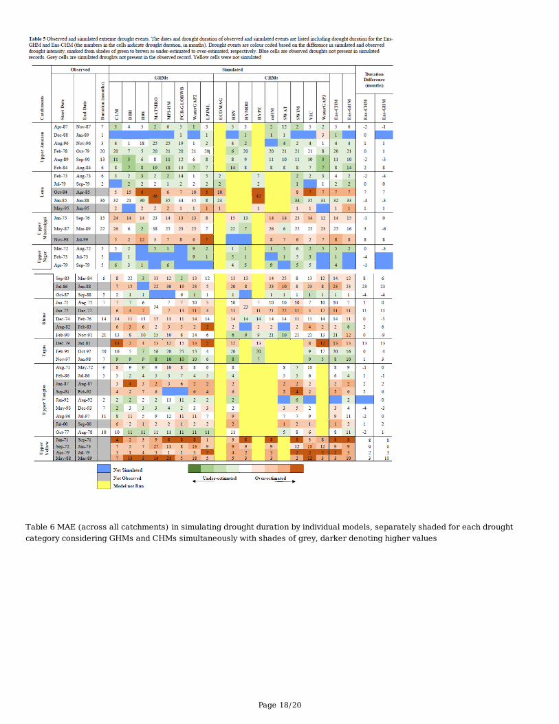
3.4. Evaluation of drought intensityTable 5 shows observed and simulated (by Ens-GHM or Ens-CHM) extreme drought events, and the performance ofindividual models in representing these events in terms of drought intensity and drought duration. In the ‘Observed’column, the observed drought events are listed from all eight catchments stating the start and end date, and droughtduration in months; unshaded cells are observed droughts, while cells shaded grey are simulated drought events that arenot present in the observed record. The respective simulated drought duration is shown in the adjacent columns. Theresults are colour-coded based on the model difference from the observed drought intensity with shades of green

Page 7/20

indicating under-estimation and brown over-estimation. Cells marked blue denote that the model did not simulate thatparticular event, while cells marked yellow indicate that the model was not run for that particular catchment.

Substantial variation was seen in the ability of individual CHMs and GHMs to simulate drought intensity. Out of the 27observed extreme drought events across all eight catchments, Ens-GHM and Ens-CHM failed to identify 3 and 1 droughtevent(s), respectively. In total 14 such extreme drought events were identi�ed by the ensemble models which were notobserved (shaded grey under ‘Observed’ in Table 5), and 5 of these events were identi�ed as extreme drought events byboth Ens-GHM and Ens-CHM.

There is a marked difference across catchments in whether the models over- or under-estimated the intensity of observeddroughts, and in the ability to simulate the very occurrence of an observed drought itself. We observed cases of falsepositive, where a model simulates a drought that never occurred in the observed record, and cases of false negative, wherea model fails to simulate a drought that occurred in the observed record for almost all catchments under extreme droughtcategory.

For the Amazon, individual CHMs and GHMs performed similarly, with most models under-estimating drought intensity of6 of the observed extreme drought events in the catchment. In one case here, an observed event went undetected by 10out of 17 models. All the individual models poorly simulated hydrological conditions in the Yellow catchment, with 4extreme drought events simulated that were not observed in reality. Model performance is more nuanced in the othercatchments, with some observed droughts within a catchment underestimated and other events over-estimated (Niger,Rhine, Yangtze).

3.5. Evaluation of drought durationFor all of the observed events which were simulated in each drought category (i.e. moderate, severe and extreme), wecalculated the absolute error in months, of the drought duration simulated by each model. The mean of all the absoluteerrors under each drought category for a model gave the mean absolute error (MAE) for that model under that particulardrought category. Figure 2 shows the MAE for the Ens-GHM and Ens-CHM, for every catchment, under the three droughtcategories along with their respective mean observed drought duration, and Table 6 presents MAE values for all individualmodels averaged across all catchments.

The largest total MAE (i.e. the MAE summed across the three drought intensity categories) was seen for the Ens-CHM forthe Niger, followed by the Mississippi and Tagus (Fig. 2). For both ensembles, the error is, overall, smallest for duration ofextreme droughts across all three drought categories Table 6. The ability of the models to simulate extreme droughtdurations better than for lower intensity drought durations is con�rmed in Fig. 2 showing the smallest magnitude of MAEfor extreme category events over half the catchments (5), across the three drought categories by Ens-CHM. For the Ens-GHM, this is the case with half the catchments (4). However, overall, it can be concluded that both the CHMs and GHMsstruggle to accurately model drought duration (errors are consistently > 1 month).

4. DiscussionThe aim of this study was to assess the performance of GHMs and CHMs in simulating observed hydrological droughtevents using the SRI as a hydrological drought indicator, computed using the observed and simulated runoff from GHMs,CHMs and respective ensemble means. No two drought events are the same and, as such, drought events cannot bejudged based on a single characteristic. Here we used three characteristics; the intensity, duration and frequency tocompare drought events. We used R2 and NSE as indicators to judge the ability of these models to replicate observedmonthly runoff and SRI patterns, and in turn identify hydrological drought events.

4.1. Comparison of simulated hydrologic conditions between GHMsand CHMs

Page 8/20

Previous studies reported that model sensitivity of CHMs and GHMs towards climate variability is comparable, andensemble models exhibit similarity in the effect of global warming on hydrological indicators (Gosling, Zaherpour, et al.2017; Hattermann et al. 2017). While R2 and NSE values (Table 2) indicated few similarities between observed monthlyrunoff and simulated runoff by GHMs; CHMs across all catchments show better reproduction of the observed monthlyrunoff except WaterGAP3 performing satisfactory in only two catchments (Rhine and Yellow). Interestingly our resultsindicate that even though the CHMs are better at reproducing better monthly runoff values, SRI series from models of bothscales are comparable (Table 3). The individual model performances also re�ected well upon both ensemble models. Ingeneral practice, evaluation of hydrological models is based on peak �ow estimations, and seldom on a model’s ability tocapture low �ow and no �ow conditions (Moriasi et al. 2007). However, for drought identi�cation it is of centralimportance that a model accurately predicts observed low-�ow and no-�ow conditions because such conditions playcritical roles in determining �ow de�cit, which accumulated over time can trigger drought events. For the purpose of thisstudy, special attention was given to extreme drought category events (events with drought intensity <-2) as they areusually the most devastating.

Although the R2 and NSE values for the SRI series are less than satisfactory for many individual GHMs and CHMs acrossalmost all catchments, the ensemble means of the two sets of models were better at estimating drought frequency formost of the catchments. There was a marked difference in performance of models when estimating drought intensityacross all catchments. One of the key reasons behind this �nding is the data used for drought identi�cation, which here isthe simulated monthly runoff data. The accuracy of the SRI output is directly proportional to the quality of data used forits calculation (Hayes et al. 1999). Huang et al. (2017) reported that CHMs accurately reproduced monthly runoff,seasonal dynamics, moderate or high �ows but simulations of low �ows were poor in most catchments. Zaherpour et al.(2018) also found that the majority of GHMs overestimated low �ows considerably more than they overestimated high-�ows and that GHMs overestimated minimum �ow return periods. The majority of the GHMs showed a tendency foroverestimating monthly runoff with a wider magnitude range (Veldkamp et al. 2018). Previous studies highlight that thiswider spread around ensembles in every catchment is due to the structure of GHMs (Haddeland et al. 2011; Gudmundssonet al. 2012). Physical processes such as transmission losses, having less presence in the GHMs is one main reason forsome of the differences between simulated and observed runoff (Gosling and Arnell 2011). In addition, evapotranspirationsimulation has been reported to vary widely among the GHMs (Wartenburger et al. 2018).

4.2. Models performance across catchmentsBoth the ensembles display, overall, a good performance comparative to the individual models and showed comparableoutputs (SRI values) despite the GHMs having a wider spread across the ensemble. The ensemble output does not alwaysdeliver better performance than individual models, however. For mean monthly runoff estimation, WaterGAP2 showedbetter results than the Ens-GHM and outperformed other GHMs because the other models overestimated orunderestimated the low-�ow conditions. The better performance of WaterGAP2 for runoff estimation can be ascribed to itscalibration with long-term annual river discharge; however, independently of calibration, the identi�cation of hydrologicalextremes remains poor among all models. Although the GHMs used the same climate forcing, they used differentformulations to compute potential evapotranspiration, which contributes to differences in simulated runoff between theGHMs (Beck et al. 2017).

Our results indicate relatively better performances of GHMs for runoff in the Rhine catchment; however, tendency towardsa false positive (Sect. 3.4) can be attributed to dry bias introduced by the choice of potential evapotranspirationformulation for individual models. For example, PCR-GLOBWB consistently appeared near the dry end of Ens-GHM,perhaps because it includes a temperature based evaporation formulation (Hamon) that has been shown to induce a largebias when applied outside its calibration range (Milly and Dunne 2017). In general, for GHMs it is di�cult to estimate adrought event at the right time because multiple errors propagate from the inputs (meteorological parameters) and some

Page 9/20

GHMs struggle to capture the magnitude and timing of processes like abstraction losses and snowmelt accurately, whichis likely to have an impact on drought timing (initiation and duration of drought events).

For CHMs, large biases have been reported in simulating low �ow conditions across a majority of studied catchmentsespecially for the Yangtze catchment (Huang et al. 2017). Similarity in performance of both sets of individual models inthe Amazon, Lena Tagus, and Yangtze catchments for intensity of extreme drought events (Table 5) can likely beattributed towards the quality of the meteorological data. Some studies have reported WATCH data to be unreliable due toinaccuracies in observed precipitation records, caused by fog/mist (Strauch et al. 2017). Secondly, the inability ofindividual CHMs to replicate low-�ow or no-�ow may be due to the choice of objective functions for calibration of theCHMs (Huang et al. 2017). In addition, inaccuracies in low-�ow observations may be a factor, or river ice effects in somecatchments, which affects estimation of drought conditions. WaterGAP3 among all CHMs comparatively showed theweakest performance, which may be attributed to fewer parameters used for model calibration compared to other CHMs.Performance of the Ens-CHM was better in some catchments than the others, likely due to the fact that different numbersof models were included for each ensemble. Therefore, one of the reasons for comparatively better performance by theEns-CHM in estimating drought frequency and lower MAE in drought duration for Rhine, Amazon and Lena is an effect ofa larger of individual models involved in the ensemble calculations.

5. ConclusionOur study focused upon the effectiveness of catchment- and global-scale hydrological models to estimate droughtconditions at the catchment scale, for 8 large catchments. We found comparably lower performance by most GHMs insimulating observed monthly runoff. R2 values for the ensemble mean SRI series varied between 0.18 and 0.95 while theNSE from − 0.14 to 0.95 across all catchments. Whilst the Ens-GHM and Ens-CHM produced similar estimates of the totalnumber of drought events across all drought categories, both ensembles struggled to estimate the frequency of droughtwithin the drought categories. Thus, both sets of models have limited ability to simulate the �ner, more granular anddetailed characteristics of observed droughts. There were marked differences across catchments in estimates of droughtintensity by models, and in ability to simulate the occurrence of observed droughts (giving false positives and falsenegatives in many cases). For both the ensembles, the error is, overall, smallest for duration of extreme droughts acrossall three drought categories. However, it can also be concluded that both CHMs and GHMs struggled in accuratelymodelling drought duration for moderate and severe drought categories. We believe that there is still room forimprovement in runoff simulations to facilitate drought identi�cation and accurate estimation of drought characteristics.Therefore, we recommend introducing multiple criteria (Krysanova et al., 2018) during model calibration speci�cally forthe evaluation of low- or no-�ow simulations.

ReferencesArnell, N. W. and Gosling, S. N. (2016) “The impacts of climate change on river �ood risk at the global scale,” ClimaticChange. doi: 10.1007/s10584-014-1084-5.

Arnold, J. G., Allen, P. M. and Bernhardt, G. (1993) “A comprehensive surface-groundwater �ow model,” Journal ofHydrology. doi: 10.1016/0022-1694(93)90004-S.

Beck, H. E. et al. (2017) “Global evaluation of runoff from 10 state-of-the-art hydrological models,” Hydrology and EarthSystem Sciences. doi: 10.5194/hess-21-2881-2017.

Beguería, S. and Vicente-Serrano, S. M. (2017) “Calculation of the Standardised Precipitation-Evapotranspiration Index(SPEI).”

Page 10/20

Bergstrom, S. and Forsman, A. (1973) “Development of a conceptual deterministic rainfall-runoff model,” NORDICHYDROL. doi: 10.2166/nh.1973.0012.

Bondeau, A. et al. (2007) “Modelling the role of agriculture for the 20th century global terrestrial carbon balance,” GlobalChange Biology. doi: 10.1111/j.1365-2486.2006.01305.x.

Boyle, D. (2001) Multicriteria calibration of hydrologic models. The University of Arizona.

Byun, H. R. and Wilhite, D. A. (1999) “Objective quanti�cation of drought severity and duration,” Journal of Climate. doi:10.1175/1520-0442(1999)012<2747:OQODSA>2.0.CO;2.

Dams, J. et al. (2015) “Multi-model approach to assess the impact of climate change on runoff,” Journal of Hydrology.doi: 10.1016/j.jhydrol.2015.08.023.

Döll, P. and Lehner, B. (2002) “Validation of a new global 30-min drainage direction map,” Journal of Hydrology, 258(1–4).doi: 10.1016/S0022-1694(01)00565-0.

Elliott, J. et al. (2014) “Constraints and potentials of future irrigation water availability on agricultural production underclimate change,” Proceedings of the National Academy of Sciences of the United States of America. doi:10.1073/pnas.1222474110.

Emerton, R. E. et al. (2016) “Continental and global scale �ood forecasting systems,” WIREs Water. doi:10.1002/wat2.1137.

Fleig, A. K. et al. (2011) “Regional hydrological drought in north-western Europe: Linking a new Regional Drought AreaIndex with weather types,” Hydrological Processes. doi: 10.1002/hyp.7644.

Frieler, K. et al. (2017) “Assessing the impacts of 1.5ĝ€°C global warming - Simulation protocol of the Inter-Sectoral ImpactModel Intercomparison Project (ISIMIP2b),” Geoscienti�c Model Development. doi: 10.5194/gmd-10-4321-2017.

Garen, D. C. (1993) “Revised Surface‐Water Supply Index for Western United States,” Journal of Water Resources Planningand Management. doi: 10.1061/(asce)0733-9496(1993)119:4(437).

Gosling, S., Zaherpour, J., et al. (2017) “A comparison of changes in river runoff from multiple global and catchment-scalehydrological models under global warming scenarios of 1 °C, 2 °C and 3 °C,” Climatic Change. doi: 10.1007/s10584-016-1773-3.

Gosling, S., Müller Schmied, H., et al. (2017) ISIMIP2a Simulation Data from Water (global) Sector. doi:10.5880/PIK.2017.010.

Gosling, S. N. and Arnell, N. W. (2011) “Simulating current global river runoff with a global hydrological model: Modelrevisions, validation, and sensitivity analysis,” Hydrological Processes. doi: 10.1002/hyp.7727.

Gudmundsson, L. et al. (2012) “Comparing large-scale hydrological model simulations to observed runoff percentiles inEurope,” Journal of Hydrometeorology. doi: 10.1175/JHM-D-11-083.1.

Haddeland, I. et al. (2011) “Multimodel estimate of the global terrestrial water balance: Setup and �rst results,” Journal ofHydrometeorology. doi: 10.1175/2011JHM1324.1.

Hagemann, S. and Dümenil, L. (1998) “A parametrization of the lateral water�ow for the global scale,” Climate Dynamics.doi: 10.1007/s003820050205.

Page 11/20

Hanasaki, N. et al. (2008) “An integrated model for the assessment of global water resources - Part 1: Model descriptionand input meteorological forcing,” Hydrology and Earth System Sciences. doi: 10.5194/hess-12-1007-2008.

Hattermann, F. F. et al. (2017) “Cross‐scale intercomparison of climate change impacts simulated by regional and globalhydrological models in eleven large river basins,” Climatic Change, 141(3), pp. 561–576. doi: 10.1007/s10584-016-1829-4.

Hayes, M. J. et al. (1999) “Monitoring the 1996 Drought Using the Standardized Precipitation Index,” Bulletin of theAmerican Meteorological Society. doi: 10.1175/1520-0477(1999)080<0429:MTDUTS>2.0.CO;2.

Heim, R. R. (2002) “A Review of Twentieth-Century Drought Indices Used in the United States,” Bulletin of the AmericanMeteorological Society, 83(8), pp. 1149–1166. doi: 10.1175/1520-0477-83.8.1149.

Huang, S. et al. (2017) “Evaluation of an ensemble of regional hydrological models in 12 large-scale river basinsworldwide,” Climatic Change. doi: 10.1007/s10584-016-1841-8.

Van Huijgevoort, M. H. J. et al. (2013) “Global multimodel analysis of drought in runoff for the second half of thetwentieth century,” Journal of Hydrometeorology. doi: 10.1175/JHM-D-12-0186.1.

Irvine, P. J. et al. (2017) “Towards a comprehensive climate impacts assessment of solar geoengineering,” Earth’s Future.doi: 10.1002/2016EF000389.

Jacobi, J. et al. (2013) “A tool for calculating the palmer drought indices,” Water Resources Research, 49(9), pp. 6086–6089. doi: 10.1002/wrcr.20342.

Keyantash, J. and Dracup, J. A. (2002) “The Quanti�cation of Drought: An Evaluation of Drought Indices,” Bulletin of theAmerican Meteorological Society. doi: 10.1175/1520-0477-83.8.1167.

Krysanova, V. et al. (2017) “ISIMIP2a Simulation Data from Water (regional) Sector.” doi: 10.5880/PIK.2018.007.

Krysanova, V. et al. (2018) “How the performance of hydrological models relates to credibility of projections under climatechange,” Hydrological Sciences Journal, 63(5). doi: 10.1080/02626667.2018.1446214.

Krysanova, V. et al. (2020) “How evaluation of global hydrological models can help to improve credibility of river dischargeprojections under climate change,” Climatic Change. doi: 10.1007/s10584-020-02840-0.

Krysanova, V. and Hattermann, F. F. (2017) “Intercomparison of climate change impacts in 12 large river basins: overviewof methods and summary of results,” Climatic Change, 141(3). doi: 10.1007/s10584-017-1919-y.

Krysanova, V., Müller-Wohlfeil, D.-I. and Becker, A. (1998) “Development and test of a spatially distributedhydrological/water quality model for mesoscale watersheds,” Ecological Modelling, 106(2–3), pp. 261–289. doi:10.1016/S0304-3800(97)00204-4.

Liang, X. et al. (1994) “A simple hydrologically based model of land surface water and energy �uxes for general circulationmodels,” Journal of Geophysical Research. doi: 10.1029/94jd00483.

Lindström, G. et al. (2010) “Development and testing of the HYPE (Hydrological Predictions for the Environment) waterquality model for different spatial scales,” Hydrology Research. doi: 10.2166/nh.2010.007.

Liu, Y. et al. (2019) “Understanding the Spatiotemporal Links Between Meteorological and Hydrological Droughts From aThree-Dimensional Perspective,” Journal of Geophysical Research: Atmospheres. doi: 10.1029/2018JD028947.

Page 12/20

Lloyd-Hughes, B. (2014) “The impracticality of a universal drought de�nition,” Theoretical and Applied Climatology. doi:10.1007/s00704-013-1025-7.

Van Loon, A. F. (2015) “Hydrological drought explained,” Wiley Interdisciplinary Reviews: Water. doi: 10.1002/wat2.1085.

McKee, T. B., Doesken, N. J. and Kliest, J. (1993) “The relationship of drought frequency and duration to time scales. InProceedings of the 8th Conference of Applied Climatology, 17-22 January, Anaheim, CA.” in Preprints, Eighth Conf. onApplied Climatology, Amer. Meteor, Soc.

Milly, P. C. D. and Dunne, K. A. (2017) “A Hydrologic Drying Bias in Water-Resource Impact Analyses of AnthropogenicClimate Change,” Journal of the American Water Resources Association. doi: 10.1111/1752-1688.12538.

Mishra, A. K. and Singh, V. P. (2010) “A review of drought concepts,” Journal of Hydrology. doi:10.1016/j.jhydrol.2010.07.012.

Moriasi, D. N. et al. (2007) “Model Evaluation Guidelines for Systematic Quanti�cation of Accuracy in WatershedSimulations,” Transactions of the ASABE, 50(3). doi: 10.13031/2013.23153.

Moriasi, D. N. et al. (2015) “Hydrologic and water quality models: Performance measures and evaluation criteria,”Transactions of the ASABE, 58(6). doi: 10.13031/trans.58.10715.

Motovilov, Y. G. et al. (1999) “Validation of a distributed hydrological model against spatial observations,” Agricultural andForest Meteorology. doi: 10.1016/S0168-1923(99)00102-1.

Muller Schmied, H. et al. (2016) “Variations of global and continental water balance components as impacted by climateforcing uncertainty and human water use,” Hydrology and Earth System Sciences, 20(7). doi: 10.5194/hess-20-2877-2016.

Nash, J. E. and Sutcliffe, J. V. (1970) “River �ow forecasting through conceptual models Part I-A discussion of principles,”Journal of Hydrology.

Oleson, K. W. et al. (2010) Technical Description of version 4.0 of the Community Land Model (CLM). doi: 10.1.1.172.7769.

Pokhrel, Y. et al. (2021) “Global terrestrial water storage and drought severity under climate change,” Nature ClimateChange. doi: 10.1038/s41558-020-00972-w.

Pokhrel, Y. N. et al. (2015) “Incorporation of groundwater pumping in a global Land Surface Model with the representationof human impacts,” Water Resources Research, 51(1). doi: 10.1002/2014WR015602.

Prudhomme, C. et al. (2014) “Hydrological droughts in the 21st century, hotspots and uncertainties from a globalmultimodel ensemble experiment,” Proceedings of the National Academy of Sciences of the United States of America. doi:10.1073/pnas.1222473110.

Samaniego, L., Kumar, R. and Attinger, S. (2010) “Multiscale parameter regionalization of a grid-based hydrologic model atthe mesoscale,” Water Resources Research, 46(5). doi: 10.1029/2008WR007327.

Shukla, S. and Wood, A. W. (2008) “Use of a standardized runoff index for characterizing hydrologic drought,” GeophysicalResearch Letters. doi: 10.1029/2007GL032487.

Strauch, M. et al. (2017) “Adjustment of global precipitation data for enhanced hydrologic modeling of tropical Andeanwatersheds,” Climatic Change. doi: 10.1007/s10584-016-1706-1.

Page 13/20

Tallaksen, L. M. L. M. et al. (2004) “Hydrological Drought: Processes and Estimation Methods for Stream�ow andGroundwater Developments in Water science,” Elsevier.

Tang, Q. et al. (2007) “The in�uence of precipitation variability and partial irrigation within grid cells on a hydrologicalsimulation,” Journal of Hydrometeorology. doi: 10.1175/JHM589.1.

UN and UNISDR, UNDP, I. (2009) Making Disaster Risk Reduction Gender Sensitive: Policy and Practical Guidelines.

Veldkamp, T. I. E. et al. (2018) “Human impact parameterizations in global hydrological models improve estimates ofmonthly discharges and hydrological extremes: A multi-model validation study,” Environmental Research Letters. doi:10.1088/1748-9326/aab96f.

Verzano, K. (2009) “Climate change impacts on �ood related hydrological processes: further development and applicationof a global scale hydrological model,” Reports on Earth System Science.

Vicente-Serrano, S. M. et al. (2012) “Accurate Computation of a Stream�ow Drought Index,” Journal of HydrologicEngineering. doi: 10.1061/(asce)he.1943-5584.0000433.

Wada, Y., Wisser, D. and Bierkens, M. F. P. (2014) “Global modeling of withdrawal, allocation and consumptive use ofsurface water and groundwater resources,” Earth System Dynamics. doi: 10.5194/esd-5-15-2014.

Wartenburger, R. et al. (2018) “Evapotranspiration simulations in ISIMIP2a-Evaluation of spatio-temporal characteristicswith a comprehensive ensemble of independent datasets,” Environmental Research Letters, 13(7). doi: 10.1088/1748-9326/aac4bb.

Weedon, G. P. et al. (2011) “Creation of the WATCH forcing data and its use to assess global and regional reference cropevaporation over land during the twentieth century,” Journal of Hydrometeorology, 12(5). doi: 10.1175/2011JHM1369.1.

Wilhite, D. A. (1993) “The Enigma of Drought,” in Drought Assessment, Management, and Planning: Theory and CaseStudies. doi: 10.1007/978-1-4615-3224-8_1.

Wilhite, D. A., Hayes, M. J. and Svoboda, M. D. (2000) “Drought Monitoring and Assessment: Status and Trends in theUnited States,” in. doi: 10.1007/978-94-015-9472-1_11.

WMO (1986) Report on Drought and Countries Affected by Drought During 1974–1985, World MeteorologicalOrganization.

Wu, J. et al. (2018) “Impacts of reservoir operations on multi-scale correlations between hydrological drought andmeteorological drought,” Journal of Hydrology. doi: 10.1016/j.jhydrol.2018.06.053.

Yevjevich, V. and Ica Yevjevich, V. (1967) “An objective approach to de�nitions and investigations of continental hydrologicdroughts an objective approach to de�nitions and investigations of continental hydrologic droughts,” Hydrology Papers.

Zaherpour, J. et al. (2018) “Worldwide evaluation of mean and extreme runoff from six global-scale hydrological modelsthat account for human impacts,” Environmental Research Letters. doi: 10.1088/1748-9326/aac547.

TablesTable 1 Catchments, gauging station, upstream area of gauging station, and the GHMs and CHMs thatcomprise ensemble (shaded)

Page 14/20

Catchment UpperAmazon

Lena UpperMississippi

UpperNiger

Rhine Tagus UpperYangtze

UpperYellow

GRDC number 3623100 2903430 4119800 1134100 6435060 6113050 --- ---

Gauging station SaoPaulo deOlivenca

Stolb Alton Koulikoro Lobith Almourol Cuntan Tangnaihai

Upstream drainage area (km2) -GRDC

990,781 2,460,000 444,185 120,000 160,800 67,490 804,859 121,000

Upstream drainage area (km2) –DDM30

994,469 2,456,513 448,575 121,058 162,092 71,007 851,303 117,543

Difference between GRDC andDDM30 areas (%)

-0.4 0.1 -1.0 -0.9 -0.8 -5.2 -5.8 2.9

GHMensemble

(Ens-GHM)

CLM (Oleson et al.2010)                

DBH (Tang et al.2007)                

H08 (Hanasaki et al.2008)                

MATSIRO (Pokhrelet al. 2015)                 

MPI-HM (Hagemannand Dümenil 1998)                

PCR-GLOBWB (Wada,

Wisser and Bierkens2014)                

WaterGAP2 (MullerSchmied et al. 2016)                LPJmL (Bondeau et

al. 2007)                Number of GHM simulations 8 8 8 8 8 8 8 8CHM

ensemble(Ens-CHM)

ECOMAG (Motovilovet al. 1999)

   

HBV (Bergstrom andForsman 1973) 

             

HYMOD (Boyle2001)

         

HYPE (Lindström etal. 2010)

     

mHM (Samaniego,Kumar and Attinger

2010)

         

SWAT (Arnold, Allenand Bernhardt 1993)

         

SWIM (Krysanova,Müller-Wohlfeil and

Becker 1998)

             

VIC (Liang et al.1994)

               

WaterGAP3 (Verzano2009)

             

Number of CHM simulations 7 5 7 7 7 4 4 6

Table 2 R2 and NSE (in parenthesis) values for simulated (individual GHMs and CHMs including both ensembles) versus observedmonthly runoff across all eight catchments. Shaded cells denotes where both R2 and NSE values are above 0.7, and marked with xdenote that the particular model was not run for the specific catchment

Page 15/20

UpperAmazon

Lena UpperMississippi

UpperNiger

Rhine Tagus UpperYangtze

UpperYellow

GHMs CLM 0.54(0.21)

0.52(0.39)

0.60(-0.40)

0.86(-2.80)

0.51(-5.30)

0.54(0.43)

0.29(0.14)

0.60(0.37)

DBH 0.60(0.48)

0.05(-0.70)

0.54(-4.40)

0.75(-4.50)

0.64(-2.80)

0.78(-1.70)

0.89(0.80)

0.78(-0.20)

H08 0.78(-0.40)

0(-0.40)

0.62(-0.10)

0.73(-6.90)

0.62(-0.90)

0.84(-1.90)

0.59(0.46)

0.58(0.36)

MATSIRO 0.49(-0.70)

0.67(0.50)

0.75(0.57)

0.88(-1.10)

0.56(0.06)

0.82(0.75)

0.77(0.57)

0.76(0.03)

MPI-HM 0.57(0.19)

0.45(0.37)

0.75(-0.30)

0.88(-1.10)

0.71(-0.90)

0.70(0.34)

0.57(0.46)

0.49(0.15)

PCR-GLOBWB

0.65(-1.20)

0.44(0.34)

0.72(0)

0.55(-0.40)

0.79(0.26)

0.84(0.79)

0.91(0.84)

0.70(-0.50)

WaterGAP2 0.76(0.73)

0.62(0.58)

0.76(0.74)

0.77 (0.75) 0.88(0.87)

0.83(0.80)

0.90(0.80)

0.64(0.53)

LPJML 0.70(-0.20)

0.50(0.28)

0.47(-0.40)

0.71(-9.10)

0.80(-1.10)

0.85(-1.60)

0.93(0.87)

0.66(0.62)

CHMs ECOMAG x 0.93(0.90)

x x x x x x

HBV 0.83(0.82)

x 0.72(0.70)

0.89 (0.77) 0.87(0.87)

0.92(0.83)

0.96(0.94)

0.84(0.82)

HYMOD 0.66(0.66)

x 0.65(0.64)

0.87 (0.86) 0.82(0.79)

x x 0.79(0.78)

HYPE x 0.95(0.94)

x x 0.90(0.85)

0.92(0.91)

x x

mHM 0.78(0.50)

x 0.89(0.86)

0.87(0.86)

0.90(0.87)

x x 0.86(0.85)

SWAT 0.78(0.62)

x 0.79(0.74)

0.85(0.72)

0.94(0.86)

x 0.94(0.93)

SWIM 0.85(0.85)

0.92(0.90)

0.78(0.77)

0.90(0.86)

0.91(0.91)

x 0.95(0.93)

0.83(0.81)

VIC 0.81(0.8)

0.85(0.80)

0.75(0.67)

0.87(0.83)

0.88(0.88)

0.88(0.85)

0.96(0.95)

0.72(0.71)

WaterGAP3 0.35(0.21)

0.44(0.39)

0.62(0.58)

0.59(0.27)

0.84(0.81)

0.79(0.66)

x 0.79(0.77)

Ens-GHM 0.81(0.24)

0.58(0.46)

0.87(0.38)

0.86(-1.70)

0.84(-0.20)

0.87(0.44)

0.83(0.79)

0.80(0.80)

Ens-CHM 0.78(0.75)

0.92(0.90)

0.89(0.89)

0.90(0.87)

0.96(0.96)

0.94(0.94)

0.97(0.96)

0.84(0.84)

Table 3 R2 and NSE (in parenthesis) values for simulated (individual GHMs and CHMs including both ensembles) versus observedSRI across all eight catchments. Shaded cells denotes where both R2 and NSE values are >0.70 and marked with x denote that theparticular model was not run for the specific catchment

Page 16/20

UpperAmazon

Lena UpperMississippi

UpperNiger

Rhine Tagus UpperYangtze

UpperYellow

GHMs CLM 0.42(0.3)

0.17(-0.29)

0.64(0.6)

0.15(-0.2)

0.5(0.43)

0.38(0.24)

0.37(0.22)

0.4(0.27)

DBH 0.44(0.34)

0.12(-0.43)

0.67(0.64)

0.11(-0.32)

0.76(0.75)

0.32(0.15)

0.45(0.35)

0.27(0.05)

H08 0.44(0.34)

0.14(-0.35)

0.66(0.63)

0.11(-0.32)

0.63(0.59)

0.31(0.13)

0.34(0.18)

0.23(-0.03)

MATSIRO 0.32(0.14)

0.3(0.01)

0.71(0.7)

0.24(-0.01)

0.55(0.49)

0.42(0.31)

0.44(0.33)

0.34(0.18)

MPI-HM 0.39(0.26)

0.19(-0.24)

0.75(0.74)

0.27(0.05)

0.71(0.7)

0.65(0.62)

0.39(0.25)

0.43(0.32)

PCR-GLOBWB

0.48(0.39)

0.33(0.06)

0.75(0.74)

0.01(-0.75)

0.8(0.79)

0.56(0.5)

0.52(0.45)

0.45(0.35)

WaterGAP2 0.53(0.47)

0.28(-0.02)

0.78(0.77)

0.24(-0.01)

0.87(0.88)

0.65(0.62)

0.54(0.48)

0.5(0.43)

LPJML 0.5(0.43)

0.12(-0.44)

0.53(0.46)

0.12(-0.28)

0.8(0.79)

0.21(-0.07)

0.47(0.37)

0.29(0.09)

CHMs ECOMAG x 0.45(0.28)

x x x x x x

HBV 0.55(0.49)

x 0.68(0.65)

0.25(0.01)

0.88(0.88)

0.75(0.74)

0.59(0.54)

0.25(0.01)

HYMOD 0.5(0.42)

x 0.59(0.54)

0.28(0.07)

0.78(0.77)

x x 0.41(0.29)

HYPE x 0.44(0.27)

x x 0.89(0.89)

0.64(0.61)

x x

mHM 0.56(0.5)

x 0.87(0.87)

0.27(0.05)

0.88(0.89)

x x 0.54(0.47)

SWAT 0.54(0.47)

x 0.72(0.7)

0.31(0.13)

0.93(0.93)

x 0.56(0.5)

x

SWIM 0.62(0.58)

x 0.73(0.72)

0.49(0.4)

0.88(0.88)

x 0.51(0.43)

0.51(0.44)

VIC 0.52(0.45)

0.3(0.01)

0.64(0.6)

0.27(0.05)

0.91(0.91)

0.34(0.18)

0.55(0.49)

0.32(0.13)

WaterGAP3 0.23(-0.02)

0.29(0)

0.77(0.76)

0.16(-0.17)

0.86(0.86)

0.57(0.51)

x 0.49(0.41)

Ens-GHM 0.56(0.5)

0.35(0.1)

0.86(0.86)

0.18(-0.14)

0.85(0.85)

0.47(0.38)

0.57(0.52)

0.56(0.46)

Ens-CHM 0.56(0.5)

0.46(0.3)

0.88(0.88)

0.33(0.15)

0.94(0.95)

0.73(0.71)

0.65(0.62)

0.53(0.46)

Table 4 Number of drought events identified from SRI series of observed and simulated Ens-GHM and Ens-CHM runoff for all eightcatchments, classified into drought categories (moderate, severe and extreme) based on drought intensity

Page 17/20

Catchments(↓)

Droughtcategory (→)

Moderate (-1 to-1.49)

Severe (-1.5 to-1.99)

Extreme Totalindividualdroughtevents(-1 or

Below)

(-2 to-2.49)

(-2.5 to-2.99)

(-3 orBelow)

Upper Amazon Ens-GHM 3 5 4 12Ens-CHM 6 5 3 1   15

Obs 6 4 3 2 1 16Lena Ens-GHM 7 4 2 1 14

Ens-CHM 7 5 2 1   15Obs 11 4 2   1 18

Upper Mississippi Ens-GHM 8 4 1 1 14

Ens-CHM 6 3 2 1   12

Obs 9 3 2     14Upper Niger Ens-GHM 10 7 1 1 19

Ens-CHM 9 4 1 1   15Obs 11 6 5     22

Rhine Ens-GHM 7 7 2 2 18Ens-CHM 8 6 3     17

Obs 10 6 3     19Tagus Ens-GHM 11 6 17

Ens-CHM 2 5 1     8Obs 5 3 1 1   10

Upper Yangtze Ens-GHM 12 5 5 22Ens-CHM 12 5 4 3   24

Obs 10 5 5 1   21Upper Yellow Ens-GHM 6 7 3 1 17

Ens-CHM 9 5 1 2   17Obs 7 9       16

Total individual drought events acrossall catchments

Ens-GHM 64 45 18 5 1 133Ens-CHM 59 38 17 9   123

Obs 69 40 21 4 2 13

Page 18/20

Table 6 MAE (across all catchments) in simulating drought duration by individual models, separately shaded for each droughtcategory considering GHMs and CHMs simultaneously with shades of grey, darker denoting higher values

Page 19/20

Drought category (SRI level) (→) Moderate(-1 to -1.49)

Severe(-1.5 to -1.99)

Extreme(-2 or Below)

Models (↓)

GHMs CLM 3.69 4.53 2.83DBH 2.3 3.5 5.29H08 2.53 3.21 6.13

MATSIRO 5.62 5.78 7.47MPI-HM 3.78 5.15 3.58

PCR-GLOBWB 3.01 4.27 3.64WaterGAP2 2.69 3.91 2.77

LPJML 2.77 2.65 6.09CHMs ECOMAG 3.63 2 5.33

HBV 3.89 4.78 3.16HYMOD 3 4.35 5.85HYPE 3.29 2.47 2.11mHM 3.5 6.15 2.36SWAT 3.11 3.51 3.78SWIM 2.8 4.28 2.38VIC 2.92 4.26 2.66

WaterGAP3 2.92 3.05 4.61  Ens-GHM 3.24 3.9 3  Ens-CHM 2.94 4.18 2.45

Figures

Figure 1

Location of the eight study catchments labelled as (1) Upper Amazon, (2) Lena, (3) Upper Mississippi, (4) Upper Niger, (5)Rhine, (6) Tagus, (7) Upper Yangtze, and (8) Upper Yellow. Note: The designations employed and the presentation of thematerial on this map do not imply the expression of any opinion whatsoever on the part of Research Square concerning

Page 20/20

the legal status of any country, territory, city or area or of its authorities, or concerning the delimitation of its frontiers orboundaries. This map has been provided by the authors.

Figure 2

MAE in simulating drought under each drought category by ensemble model (Ens-GHM and Ens-CHM) for all eightcatchments along with respective mean observed drought duration