Acoustic Waves in Layered Media - From Theory to Seismic
52
1 Acoustic Waves in Layered Media - From Theory to Seismic Applications Alexey Stovas 1 and Yury Roganov 2 1 NTNU, Trondheim, 2 USGPI, Kiev, 1 Norway 2 Ukraine 1. Introduction Acoustic wave propagation in layered media is very important topic for many practical applications including medicine, optics and applied geophysics. The key parameter controlling all effects in layered media is the scaling factor given by the ratio between the wavelength and the layer thickness. Existing theory mostly covers the solutions derived for the low-frequency and high-frequency limits. In the first limit, when the wavelength is much larger than the layer thickness, the layered medium is substituted by an effective medium with the properties given by special technique called the Backus averaging. In the second limit, when the wavelength is much smaller than the layer thickness, we can use the ray theory to compute both reflection and transmission responses. In practice, the wavelength could be comparable with the layer thickness, and application of both frequency limits is no longer valid. In this chapter, we will mainly focus on the frequency-dependent effects for acoustic waves propagating through the layered media. We show that there are distinct periodically repeated patterns consisted of the pass- and stop-bands of very complicated configuration defined in frequency-slowness or frequency- group angle domain that control the reflection and transmission responses. The edges between the pass- and stop-bands result in the caustics in the group domain. The quasi- shear waves in a homogeneous transversely isotropic medium could also results in the high- frequency caustics, but for the layered media, all wave modes can result in frequency- dependent caustics. The caustics computed for a specific frequency differ from those observed at the low- and high-frequency limits. From physics point of view, the pass-bands correspond to the effective medium, while the stop-bands correspond to the resonant medium. We distinguish between the effects of scattering and intrinsic attenuation in layered media. The propagation of acoustic waves in a layered medium results in the energy loss due to scattering effect. The intrinsic attenuation is an additional effect which plays very important role in seismic data inversion. We provide the theoretical and numerical study to compare both effects for a periodically layered medium. We also investigate the complex frequency roots of the reflection/transmission responses. We also derive the phase velocity approximations in a layered medium. As the trial model for layered medium, we widely use the periodically layered medium with the limited number of parameters. The propagation of acoustic waves through a periodic layered medium is analyzed by an eigenvalue www.intechopen.com
Transcript of Acoustic Waves in Layered Media - From Theory to Seismic

1
Acoustic Waves in Layered Media - From Theory to Seismic Applications
Alexey Stovas1 and Yury Roganov2 1NTNU, Trondheim,
2USGPI, Kiev, 1Norway 2Ukraine
1. Introduction
Acoustic wave propagation in layered media is very important topic for many practical applications including medicine, optics and applied geophysics. The key parameter controlling all effects in layered media is the scaling factor given by the ratio between the wavelength and the layer thickness. Existing theory mostly covers the solutions derived for the low-frequency and high-frequency limits. In the first limit, when the wavelength is much larger than the layer thickness, the layered medium is substituted by an effective medium with the properties given by special technique called the Backus averaging. In the second limit, when the wavelength is much smaller than the layer thickness, we can use the ray theory to compute both reflection and transmission responses. In practice, the wavelength could be comparable with the layer thickness, and application of both frequency limits is no longer valid. In this chapter, we will mainly focus on the frequency-dependent effects for acoustic waves propagating through the layered media. We show that there are distinct periodically repeated patterns consisted of the pass- and stop-bands of very complicated configuration defined in frequency-slowness or frequency-group angle domain that control the reflection and transmission responses. The edges between the pass- and stop-bands result in the caustics in the group domain. The quasi-shear waves in a homogeneous transversely isotropic medium could also results in the high-frequency caustics, but for the layered media, all wave modes can result in frequency-dependent caustics. The caustics computed for a specific frequency differ from those observed at the low- and high-frequency limits. From physics point of view, the pass-bands correspond to the effective medium, while the stop-bands correspond to the resonant medium. We distinguish between the effects of scattering and intrinsic attenuation in layered media. The propagation of acoustic waves in a layered medium results in the energy loss due to scattering effect. The intrinsic attenuation is an additional effect which plays very important role in seismic data inversion. We provide the theoretical and numerical study to compare both effects for a periodically layered medium. We also investigate the complex frequency roots of the reflection/transmission responses. We also derive the phase velocity approximations in a layered medium. As the trial model for layered medium, we widely use the periodically layered medium with the limited number of parameters. The propagation of acoustic waves through a periodic layered medium is analyzed by an eigenvalue
www.intechopen.com

Waves in Fluids and Solids
4
decomposition of the propagator matrix. This reveals how the velocity and attenuation of the layered medium vary as function of the periodic structure, material parameters and frequency. We show that there is one more parameter controlling the wave propagation apart of the wavelength to layer thickness ratio that is the acoustic contrast between the layers. Multiple scattering in finely layered sediments is important in stratigraphic interpretation in seismic, matching of well log-data with seismic data and seismic modelling. Two methods have been used to treat this problem in seismic applications: the O’Doherty-Anstey approximation and Backus averaging. The O’Doherty-Anstey approximation describes the stratigraphic filtering effects, while the Backus averaging defines the elastic properties for an effective medium from the stack of the layers. Using numerical examples, we show that there is a transition zone between the effective medium (low-frequency limit) and the time-average medium (high-frequency limit) and that the width of this zone depends on the strength of the reflection coefficient series. Assuming that a tubidite reservoir can be approximated by a stack of thin shale-sand layers we use standard AVO-attributes to estimate net-to-gross and oil saturation. Necessary input is Gassmann rock physics properties for sand and shale as well as the fluid properties for hydrocarbons. Required seismic input is AVO intercept and gradient. The method is based upon thin layer reflectivity modeling. It is shown that random variability in thickness and seismic properties of the thin sand and shale layers does not change the AVO attributes at top and base of the turbidite reservoir sequence significantly. The method is tested on seismic data from offshore Brazil, and the results show reasonable agreement between estimated and observed net-to-gross and oil saturation. The methodology can be further developed for estimating changes in pay thickness from time lapse seismic data. We propose the method of computation seismic AVO attributes (intercept and gradient) from ultra-thin geological model based on the SBED modelling software. The SBED software is based on manipulating sine-functions, creating surfaces representing incremental sedimentation. Displacement of the surfaces creates a three dimensional image mimicking bedform migration, and depositional environments as diverse as tidal channels and mass flows can be accurately recreated. The resulting modelled deposit volume may be populated with petrophysical information, creating intrinsic properties such as porosity and permeability (both vertical and horizontal). The Backus averaging technique is used for up-scaling within the centimetre scale (the intrinsic net-to-gross value controls the acoustic properties of the ultra-thin layers). It results in pseudo-log data including the intrinsic anisotropy parameters. The synthetic seismic modelling is given by the matrix propagator method allows us to take into account all pure mode multiples, and resulting AVO attributes become frequency dependent. Within this ultra-thin model we can test different fluid saturation scenarios and quantify the likelihood of possible composite analogues. This modelling can also be used for inversion of real seismic data into net-to-gross and fluid saturation for ultra-thin reservoirs. There are many other issues related to wave propagation in layered media we do not discuss in
this chapter. For further reading we suggest several books (Aki&Richards, 1980; Brekhovskih,
1960; Kennett, 1983; Tsvankin, 1995) that cover the problems we did not touch here.
2. System of differential equations
To describe the dynamic of the wave propagation in an elastic medium, it is common to use the Hook’s law that defines the linear relation between the stress tensor ij and the strains tensor pqe ,
www.intechopen.com
Acoustic Waves in Layered Media - From Theory to Seismic Applications
5
ij ijpq pqc e , (1)
where 1
2
p q
pq
q p
u ue
x x
and ijpqc is the stiffness tensor. If there are no volume forces
within the medium, we can write the moment equation in the following way (Aki and Richards, 1980)
2
2
iji
j
u
t x
. (2)
In equation (1) and (2), it is assumed that the summation is performed over the repeatable indices. Since the tensor ijpqc is symmetrical with respect to index changing ij pq , i j , p q , the relation (1) can be written as
p
ij ijpq
q
uc
x . (3)
If we denote ii
uv
t
as the velocity of the particle movement, the equations (2) and (3) can
be given as
iji
j
v
t x
, (4)
ij p
ijpq
q
vc
t x
. (5)
We can apply the Fourier transform for the variables , 1x , 2x to equations (4) and (5) according to the following relations
1 1 2 2
1 2 1 2 1 23
1, , , ,
8
i p x p x tf p p f x x t e dx dx dt
,
1 1 2 22
1 2 1 2 1 2, , , ,i p x p x t
f x x t f p p e dp dp d
.
After substituting the derivatives on 1x , 2x , t with the coefficients 1i p , 2i p , i , and excluding the variables 11 , 12 , 22 , the system of equations (4)-(5) can be given in a vector-matrix form
di
dzbMb , (6)
where vector 1 2 3 13 23 33, , , , ,T
v v v b , 3z x , and matrix M is defined as
1
33
T
A C
MB A
, (7)
www.intechopen.com

Waves in Fluids and Solids
6
with ,,mn mp nqp q cC , 1
33 1 31 2 32p p A C C C and 1
3 33 3
, 1,2
m n m n mn
m n
p p
B C C C C I ,
where 1p and 2p are the horizontal slowness in 1x and 2x direction, respectively, and is
the density. The matrices 1
33
C and B are symmetrical, and matrix M satisfies the equation
TKMK M , (8)
where TM is transposed matrix,
0 I
KI 0
and I is the unit 3x3 matrix. Equation (6)
describes the wave propagation in the vertically heterogeneous medium with all parameters
being dependent on z-coordinate only. Note, even if the parameters z and ijpqc z are
discontinuous functions, the components of the vector b remain continuous functions of
depth. If the medium is a homogeneous transversely isotropic with vertical symmetry axis (a VTI medium), the propagation of waves in qP-qSV system is independent from the qSH-waves propagation. In this case, there are two equations (6): with dimension 4x4 (qP-qSV system) and with dimension 2x2 (qSH wave). For vertical propagation, equation (6) is reduced into three independent equations (for qP-, qSV- and qSH-waves). The analytical
form of matrix M for different types of media can be found in Aki and Richards (1980), Braga and Herrmann (1992) and Fryer and Frazer (1987).
3. Propagator matrix
The propagator matrix is the matrix 0 6,z z P GL C that is the solution of initial-value
problem
0
0
,,
z zi z z
z
PMP , 0 0,z z P I . (9)
The propagator matrix satisfies the Volterra integral equation
0
0 0, ,
z
z
z z z d P I M P , (10)
that can be solved by using the Picard iteration. This leads to the Peano series for 0,z zP
(Peano, 1888; Pease, 1965)
1
0 0 0
0 1 1 1 2 2 1, ...
z z
z z z
z z d d d
P I M M M . (11)
The series (11) converges if c M for all 0 ,z z , where ... is some matrix norm. If M M , the matrix with constant elements, than equation (11) is reduced to the exponent
0 0, expz z i z z P M . (12)
From equation (9), it follows that for any vector 0zb , the vector 0 0,z z z zb P b is the
solution of equation (6). By substituting the basis vectors ie , 1,2,3i , instead of the vector
www.intechopen.com

Acoustic Waves in Layered Media - From Theory to Seismic Applications
7
0zb , we can prove that the columns of matrix 0,z zP are the linear independent
solutions of equation (6), i.e. the propagator matrix describes the fundamental system of
solutions of equation (6). Since,
2 2 0 0 2 1 1 0 0, , ,z z z z z z z z z b P b P P b , (13)
than,
2 0 2 1 1 0, , ,z z z z z zP P P . (14)
If the medium consists of N layers with matrices iM and layer thickness ih , the equations
(12)-(14) gives the propagator matrix from the stack of the layers
0 1 1, exp ...expN N Nz z i h i h P M M , (15)
where 0 1 ...N Nz z h h .
Equation (15) was used by Haskell (1953) and Thomson (1950) in their works to describe the wave propagation in a layered isotropic medium.
4. Symmetry relations
Let us assume that matrices k
M can be diagonalized by using a similarity transformation, ( ) 1
diagm
k k k k M E E . In this case, ( ) 1
exp diag expm
k k k k k ki h i h M E E . The
columns of matrix k
E are the polarization vectors for all types of wave propagating in layer
k with horizontal slownesses 1p and
2p , while
( )m
k are corresponding vertical slownesses.
Therefore, the vector 1
( ) ( )k
z zw E b consists of up- and down-going wave amplitudes in
layer k with 1 1 1
... ...k k
h h z h h . Let us denote by 0
E and 1N E the matrices that
consist of the eigen-vectors of matrices 0
M and 1N M , respectively, which define the
properties of the half-spaces surrounding the stack of layers. The matrix
1
1 0
NQ E PE (16)
is called the amplitude propagator matrix, since the equation 1 0N w Qw provides the
linear relation between the amplitudes over and under the stack of layers for all wave types.
The amplitude propagator matrix can be blocked by 3x3 sub-matrices, 1,2ij ijQ Q , and the
amplitude vectors 0
w and 1N w can be blocked by three-component sub-vectors,
corresponding to up- and down-going waves of different type,
0
0
0
u
wd
, 1
1
1
N
N
N
uw
d. (17)
Therefore, we can write
1 011 21
1 021 22
N
N
u uQ Q
d dQ Q. (18)
www.intechopen.com

Waves in Fluids and Solids
8
From equation (18), it follows that the amplitudes of waves going away from the stack of
layers: 0
u and 1N d can be computed from the amplitudes of waves coming to the stack of
layers: 1N u and
0d ,
1 0
0 1
N D U
D U N
d T R d
u R T u, (19)
where
1
22 21 11 12D
T Q Q Q Q , (20)
1
21 11U
R Q Q , (21)
1
11 12D
R Q Q , (22)
1
11U
T Q . (23)
The matrices U
R , U
T and, D
R ,D
T are called the reflection and transmission matrices for up-
and down-going wave, respectively (Figure 1). From equations (20)-(23), the amplitude
propagator matrix can be rewritten as
1 1
1 1
U U D
U U D U U D
T T RQ
R T T R T R
. (24)
The matrix
D U
D U
T R
SR T
(25)
is called the scattering matrix (Ursin, 1983) and contains all reflection and transmission
coefficients for up- and down-going waves of all type as sub-matrices. If the layers posses the
VTI (transverse isotropy with vertical symmetry axis) symmetry, the following relation is valid
T Q JQ J , (26)
where 0 I
JI 0
. In order to prove the relation (26), we represent the amplitude
propagator matrix Q as 1 0
...N N
Q F Λ Λ F , where 1
1k k k
F E E , ( )
diagm
k kΛ and ( ) ( )
expm m
k k ki h . To validate the relation (26), it is sufficient to prove that
T
k k Λ J J
and T
k kF JF J . The first equality follows from the fact that the matrix
kΛ is diagonal, and
the elements of matrix k
Λ are symmetric, ( 3 ) ( )
1m m
k k . The second equality can be proven
by substitution of equations (35) and (36) for matrices k
E and 1
1k
E into this equation and
www.intechopen.com

Acoustic Waves in Layered Media - From Theory to Seismic Applications
9
using relations (37). The symmetry relations for reflection and transmission matrices for
stack of layers sandwiched between two half-spaces,
T
D DR R ,
T
U UR R ,
T
D UT T , (27)
can be derived by substitution the expression for amplitude propagator matrix Q from
equation (24) into equation (26). It is assumed that all layers and half-spaces posses the VTI
symmetry, and the presence of attenuation is allowed. The symmetry relations (27) are also
derived by Ursin (1983) for a stack of isotropic layers. If we consider the single interface
between the half-spaces, than the diagonal sub-matrices in equation (24) are equal (see
equations (35) and (36)), and, therefore, 1 1
U U U D
R T T R and 1 1
U D U U D
T T R T R (Ursin,
1983). These relations result in
0U U D U
T R R T , 2
D U U T T R I . (28)
By using 1
U U D U
R T R T and equations (27) we can derive two additional symmetry
relations
0U D D D
R T T R , 2
U D D T T R I . (29)
The symmetry relations (28) and (29) are derived by Frasier (1970), Kennett et al. (1978) and Ursin (1983).
5. Reflection and transmission responses of layered transversely isotropic media
This chapter is mostly based on the paper Stovas and Ursin (2003). The major point in this
chapter is wave field decomposion into up- and down-going waves (Kennett, 1983; Ursin,
1983) scaled such that, for an elastic medium, the vertical energy flux is constant. This
results in important symmetries in the transformation matrix and also in the reflection and
transmission (R/T) coefficients (Chapman, 1994; Ursin and Haugen, 1996). The equations of
motion and Hook’s law in a source free VTI medium (radially symmetric about the vertical,
z axis) for qP- and qSV-waves in 1 3X X plane after applying a Fourier transform can be
expressed as an ordinary first-order matrix-vector differential equation as shown in
equation (6), where denotes circular frequency, 3 13 33 1, , ,T
v v b is the displacement
velocity - stress vector, the superscript " "T indicating the transpose, and the matrix M has
the blocked structure,
0
0
A
MB
, (30)
composed of the 2x2 symmetric matrices A and B are given by
1 1
33 13 33
11 2 2 15513 33 11 13 33
,c pc c p
p cpc c p c c c
A B , (31)
www.intechopen.com

Waves in Fluids and Solids
10
which are dependent on the horizontal slowness p , the stiffness coefficients ijc from the stiffness matrix and the density . In order to decompose into up- and down-going waves (Ursin, 1983, Ursin and Stovas, 2002), we make the linear transformation
u
b Ed
. (32)
Then equation (6) becomes
id
idz
u Δ 0 F G u
d 0 Δ G F d, (33)
where u and d are the up- and down-going wave amplitudes, and
,qP qSVdiag Δ (34)
contains the vertical slownesses for qP- and qSV-waves, qP and qSV . The transformation matrix
1 1
2 2
1
2
E E
EE E
(35)
is normalized with respect to the vertical energy flux so that the inverse has the simple form
1 1 T T
1 1 2 2 1
1 1 T T
1 2 2 1
1 1
2 2
E E E E
EE E E E
. (36)
Matrices 1E and 2E posses the symmetries
2 1 2 1
T T E E E E I . (37)
Therefore, the layer propagator matrix can be given as
( ) ( )
1 11 12
( ) ( )
21 11
exp expk k
k k k k
ii h i h
i
P PP M E Λ E
P P, (38)
where ( ) 1cosk
mm m mh P E Δ E and ( ) 1sink
mn m nh P E Δ E , , , 1,2m n m n . From equation (37)
and (38), it follows that
( ) ( )
1 1 11 12
( ) ( )
21 11
exp expk k
k k k k
ii h i h
i
P PP M E Λ E
P P, (39)
and
( ) 1 1 ( )
11 1 1 2 2 22
( ) 1 1 ( )
21 2 1 2 1 21
( ) 1 1 ( )
12 1 2 1 2 12
cos cos
sin sin
sin sin
TTk k
TTk k
TTk k
h h
h h
h h
P E Δ E E Δ E P
P E Δ E E Δ E P
P E Δ E E Δ E P
. (40)
www.intechopen.com

Acoustic Waves in Layered Media - From Theory to Seismic Applications
11
The product of matrices of this type indicates that the propagator matrix P for the stack of layers can be blocked as follows
11 12
21 22
i
i
P P
PP P
, (41)
where the elements of 2x2 matrices klP are real functions of horizontal slowness p and
frequency . The elements of matrices kl P are even/odd functions of frequency if k+l is
an even/odd number, respectively. Matrix kM possesses the following symmetries
,T
k k k k KM K M TM T M , (42)
where I 0
T0 I
. Therefore,
1exp , expT T
k k k k k ki h i h KP K M P TP T M P . (43)
For an elastic medium, the elements of matrix kM are real, and, therefore, * 1
k k
P P , and equations (43) can be rewritten as
* *,T
k k k k
KP K P TP T P . (44)
Multiplications of equations (44) for 1,...,k N , gives similar symmetry relations for propagator matrix for the stack of layers,
* *,T KPK P TPT P . (45)
The scattering matrices F and G are given by
1 2 1 22 1 2 1
1 1,
2 2
T T T Td d d d
dz dz dz dz
E E L E
F E E G E E , (46)
with symmetries
,T T F F G G , (47)
so that F and G have the form
11 12
12 22
0,
0
g gf
g gf
F G . (48)
To compute the scattering matrices F and G , we express them as functions of
perturbations in the elements of the matrices A and B in equation (31). The eigenvector
matrices satisfy the following equations
2 1 1 2, AE E Δ BE E Δ . (49)
From equations (35) and (36), we obtain
www.intechopen.com

Waves in Fluids and Solids
12
1 1 2 2, E E G F E E G F . (50)
Differentiating equations (49) and substituting equations (50), we obtain
11 12
2 2 1 1
12 22
2 2 1 1
2 1
22
0 1
20
qP qP qSVT T
qP qSV qSV
qP qSV T T
qP qSV
g g
g g
f
f
ΔG GΔ E A E E B E
ΔF FΔ E AE E B E Δ
. (51)
From equations (51) we can compute all elements of matrices F and G . Equation (6) can be solved not only by propagator matrix technique described in previous chapter, but also by a layer-recursive scheme described in Ursin and Stovas (2002). We let
DjR , DjT , UjR and UjT denote the R/T matrices for the interface at jz z (Figure 1). For the layer thickness 1j j jz z z , the layer propagator matrix is given by
expj j ji z L Λ . (52)
Assume that the generalized reflection matrix from the top of layer j+1 to the bottom of the stratified medium, ,D j Nz z
R , is known; then the new reflection matrix up to the top of layer j is given by the recursive relation (Ursin, 1983)
1
1, , ,D j N j Dj Uj D j N Dj D j N Dj jz z z z z z R L R T R I R R T L . (53)
It is started with the initial value , 0D j Nz z R , satisfying the radiation condition in the elastic half-space. By considering a plane interface between two homogeneous media, we can define the transmission and reflection coefficient matrices. Continuity of the wavefields gives the 2x2 reflection and transmission matrices (Ursin, 1983):
1 12 ,
DPP DPS DPP DPS
D D
DSP DSS DSP DSS
t t r r
t t r r
T C D R C D C D , (54)
with
1 2 1 2
2 1 1 2,T T C E E D E E , (55)
where superscripts 1
and 2
denote the upper and lower medium, respectively.
RD
TD
TU
RU
I
I
zz
00
Fig. 1. Definition of the reflection and transmission response matrices (Ursin&Stovas, 2002).
www.intechopen.com

Acoustic Waves in Layered Media - From Theory to Seismic Applications
13
The symmetry equations (37) imply that
T CD I . (56)
Using equation (55), the reflection and transmission matrices are given by
11 22 21 12
12 21 22 11
2 2 2 2 2
11 12 21 22 11 21 12 22
2 2 2 2 2
11 21 12 22 11 12 21 22
det det2
det detdet( )det
det 1 21
det( )det 2 det 1
D
D
c c c c
c c c c
c c c c c c c c
c c c c c c c c
C CT
C CC D C
CR
C D C C
(57)
where ijc are elements of matrix C and
2 2 2 2 2
11 12 21 22det det det 1 c c c c C D C C . (58)
The matrices UR and UT can be computed by interchanging the superscripts 1 and 2 or
using the symmetry relations (37) and (56) (Ursin and Stovas, 2001), which gives
1,T
U D U D D D
T T R T R T . (59)
The weak-contrast approximations for reflection and transmission matrices an be derived by
assuming weak contrast in elastic parameters above and below the interface. We consider a
plane interface with a discontinuity in the parameters
2 1
k k km m m (60)
and average parameters
2 1
2
k kk
m mm
, (61)
where 1
km and 2
km characterize the medium above and below the interface, respectively.
To approximate the reflection and transmission matrices in equation (54), we proceed as in
Stovas and Ursin (2001) and expand the matrices , 1,2, 1,2
j
k k j E , into second-order
Taylor series with respect to the average medium. This gives the second-order approximations
2 2 2
11 12 12 11 22 11 12 12 11 222 2
2 2 2
12 11 22 12 22 12 11 22 22 12
1 1 11
2 2 2,
1 1 11
2 2 2
D D
g g f f g g g g g f g f g g
f g g g g g f g f g g g g f
T R
. (62)
From the symmetries of the matrices 1E and 2E , the second-order derivatives of these
matrices with respect to the medium parameters cancel; therefore they do not appear in the
second-order approximations for the R/T coefficients. In the equations above, the elements
f and ijg are as defined in equation (46), but the derivatives of the medium parameters
kdm
dz are replaced by km . Neglecting the second-order terms gives the linear approximations
www.intechopen.com

Waves in Fluids and Solids
14
1 1,D D T I F R G . (63)
These correspond to ones given in Ursin and Haugen (1996) for VTI media and in Aki and
Richards (1980) for isotropic media, except that they are normalized with respect to the
vertical energy flux and not with respect to amplitude.
6. Periodically layered media
Let us introduce the infinite periodically layered VTI medium with the period thickness
1
N
j
j
H h
, where
jh is the thickness of
th
j layer in the sequence of N layers comprising the
period. The dispersion equation for this N layered medium is given by (Helbig, 1984)
det exp 0i H P I , (64)
and the period propagator matrix P is specified by formula (15). The equation (64) is known
as the Floquet (1883) equation.
The parameter ,p is effective and generally complex vertical component of the
slowness vector. For plane waves with horizontal slowness p , the real part of which satisfies
equation (64), Re q , defines the vertical slowness of the envelope, while the imaginary part,
Im , characterizes the attenuation due to scattering. Note that for propagating waves,
0
lim 0
. This indicates that there is no scattering in the low frequency limit.
The low and high frequency limits
In the low-frequency asymptotic of the propagator matrix P has the following form exp i H P M with
2
1
1
2
N
k k j j j
k j
ih h h o
H H
M M M M M M
(65)
Therefore, the dispersion equation (64) in the low-frequency limit has roots similar to those defined for a homogeneous VTI medium given by the averaged matrix
1
10
N
k k
k
hH
M M . (66)
One can see from observing the elements of the matrices in equation (31) that equation (66)
is equivalent to the Backus averaging. The propagator matrix P , which defines the
propagation of mode k
m in the th
k layer, 1, ...,k N , can be defined as
1 1
exp exp expN N k k
i h i h i h P F F F , (67)
where ( ) ( ) ( )
k k km m m T
k k k kF n m is a 4x4 matrix of rank one,
( )k
m T
km and
( )k
m
kn are the left- and right
hand side eigenvectors of matrix k
M with eigenvalue ( )m
k . Substituting
kF into equation (67)
results in
www.intechopen.com

Acoustic Waves in Layered Media - From Theory to Seismic Applications
15
1 1 1
1 1 1
1 1
exp ... expT T T
k N N k N
N N
m m m m mm m m
k k N N k k N
k k
i h i h
P n m n m n m , (68)
where the number 1( ) ( )
1ln ...N
m T m
N m n . In this case, the dispersion equation (64), which
defines the vertical slowness for the period of the layered medium, has the root given by
1
1k
N
m
k k
k
ih
H H
, (69)
where the term i H is responsible for the transmission losses for propagating waves
which is frequency independent. This can be shown by considering the single mode plane
wave,
exp exp expi pr z t i pr q z t z H , (70)
where
1
1k
N
m
k k
k
q h qH
. (71)
This equation defines the vertical slowness for a single mode transmitted wave initiated by a
wide-band - pulse, since it is frequency-independent. The caustics from multi-layered VTI
medium in high-frequency limits are discussed in Roganov and Stovas (2010). Note, that
propagator matrix in equation (68) describes the downward plane wave propagation of a
given mode within each layer, i.e. the part of the full wave field. All multiple reflections and
transmissions of other modes are ignored. Therefore, this notation is valid for the case of the
frequency independent single mode propagation of a wide band pulse. In the low
frequency limit, the wave field consists of the envelope with all wave modes. For an
accurate description of this envelope and obtaining the Backus limit we have to use the
formula (15) for complete propagator P .
6.1 Dispersion equation analysis
From the relations (45), one can see that the matrices P , *P and *
TP are similar. These
matrices have the same eigen-values. So, if x is eigen-value of matrix P , than *x , 1x and *1x are also eigen-values. Additionally, taking into account the identity, det 1P , it can
be shown, that equation
det 0x P I (72)
reduces to
21 1
1 2 2 0x x a x x a , (73)
and the roots of equation (64) corresponding to qP- and qSV-waves, P and S , satisfy
the equations
www.intechopen.com

Waves in Fluids and Solids
16
1 2
1 1 1cos cos , , cos cos , .
2 4 2qP qSV qP qSVH H a p H H a p (74)
The real functions 1 ,a p and 2 ,a p can be computed using the trace and the sum of
the principal second order minors of the matrix P , respectively. Using equation (41) and
taking into account that 11 P and 22 P are even functions of frequency, and 12 P and 21 P are odd functions of frequency, the functions 1 ,a p and 2 ,a p are even
functions of frequency and horizontal slowness. The system of equations (74) defines the
continuous branches of functions Re ,qP qPq p and Re ,qSV qSVq p which
specify the vertical slowness of four envelopes with horizontal slowness p and frequency
. Let us denote 1 1, , 4b p a p , 2 2, , 4 1 2b p a p and 1
2
x xy
. Note that
the functions 1 ,b p and 2 ,b p are also even functions of frequency and horizontal
slowness.
-1.5 -1.0 -0.5 0.0 0.5 1.0 1.5
-2.0
-1.5
-1.0
-0.5
0.0
0.5
1.0
1.5
2.0
M3
M2
M1
M0
N2N
1
f=25Hz
f=50Hz f=15Hz
2
435
1
1,2: no roots
3: one root (qP)
4: one root (qSV)
5: two roots
b2
b1
Fig. 2. Propagating and evanescent regions for qP and qSV waves in the 1 2,b b domain.
The points 1
1,1N and 2
1,1N denote the crossings between 2 1
1 2b b and 2
2 1b b .
The paths corresponding to f const are given for frequencies of 15, 25 and 50f Hz are
shown in magenta, red and blue, respectively. The starting point 0
M (that corresponds to zero
horizontal slowness) and the points corresponding to crossings of the path and boundaries
between the propagating regions, , 1, 2, 3j
M j , are shown for the frequency 15f Hz .
Points 4
M and 5
M are outside of the plotting area (Roganov&Stovas, 2011).
All envelopes are propagating, if the roots of quadratic equation
2
1 22 0y b y b (75)
are such that 1 1y and 2 1y . On the boundaries between propagating and evanescent
envelopes, we have 1y or discriminator of equation (75), 21 2, 0D p b b . In the
first case we have, 2 11 2b b , and in the second case, 2
2 1b b (Figure 2). If 1y , the
equation cosy H has the following solutions
www.intechopen.com

Acoustic Waves in Layered Media - From Theory to Seismic Applications
17
2
2
12 ln 1 , , 1
1(2 1) ln 1 , , 1
n i y y n yH
n i y y n yH
Z
Z
, (76)
and Req const in this area. The straight lines 2 11 2b b and the parabola 2
2 1b b
defined between the tangent points 1 1,1N and 2 1,1N split the coordinate plane 1 2,b b
into five regions (Figure 2). If parameters 1b and 2b are such that the corresponding point 1 2,b b is located in region 1 or 2, the system of equations (74) has no real roots, and
corresponding envelopes do not contain the propagating wave modes. The envelopes with
one propagating wave of qP-or qSV- wave mode correspond to the points located in region
3 or region 4, respectively. The points from region 5 result in envelopes with both
propagating qP- and qSV-wave modes. If a specific frequency is chosen, for instance,
30 Hz (or 15f Hz ), and only the horizontal slowness is varied, the point with
coordinates 1 2,b b will move along some curve passing through the different regions.
Consequently, the number of propagating wave modes will be changed. In Figure 2, we
show using the points iM 0, 5i with the initial position 0M defined by 0p and the
following positions crossing the boundaries for the regions occurred at 1 0.172p s km ,
2 0.217p s km and 3 0.246p s km . This curve will also cross the line 2 11 2b b at
4 0.332p s km and 5 0.344p s km . Between the last two points, the curve is located in the
region 2 with no propagating waves for both modes. The frequency dependent positions of
the stop bands for p const can be investigated using the curve, 1 2,b b b .
Since the propagator in the zero frequency limit is given by the identity matrix, 0
lim P I , than 1 20 0 1b b , and all curves b start at the point 2 1,1N . For
propagating waves, the functions 1b and 2b are given by linear combinations of
trigonometric functions and therefore are defined only in a limited area in the 1 2,b b
domain.
-1.0 -0.5 0.0 0.5 1.0
-1.0
-0.5
0.0
0.5
1.0
co
s(
P)
cos(S)
-1.0 -0.5 0.0 0.5 1.0
-1.0
-0.5
0.0
0.5
1.0
b2
b1
Fig. 3. The normal incidence case ( 0p ). The dependence of cosqP
H on cosqSV
H
(a Lissajous curve) is shown (left) and similar curve is plotted in the 1 2,b b domain (right).
Both of these plots correspond to frequency range 0 50Hz . Note, that the stop bands exist
only for qP wave and can be seen for cos 1qP
H in the left plot and for
2 11 2b b in the right one (Roganov&Stovas, 2011).
www.intechopen.com

Waves in Fluids and Solids
18
The simplest case occurs at the normal incidence where 0p . At this point the quadratic
equation 2
1 22 0y b y b has two real roots qPy and qSVy for each value
of . The functions cosqP qPy H and cosqSV qSVy H are the right side of
the dispersion equation for qP- and qSV- wave, respectively. If these trigonometric
functions have incommensurable periods, the parametric curve ,qSV qPy y densely
fills the area that contains rectangle 1,1 1,1 and is defined as a Lissajous curve
(Figure 3, left). The mapping , ,2
qSV qPqSV qP qSV qP
y yy y y y
has the Jacobian
2
qSV qPy y with a singularity at qSV qPy y . This point is located at the discriminant
curve, 2
2 1b b . We can prove that the curve ,
2
qSV qPqSV qP
y yy y
is tangent
to parabola 2
2 1b b at the singular point and is always located in the region 2
2 1b b . In fact,
i f , 1
2
qSV qPy yb
, 2 qSV qPb y y a n d 0 0qP qSVy y t h a n
22
1 2 0
10
4qP qSVb b y y . In Figure 3 ( left) , i t is shown the
parametric curve ,qSV qPy y computed for our two layer model described in Table 1.
Since both layers have the same vertical shear wave velocity and density, cosqSV qSVy t with 1 2 0qSVt h h . In the qP- wave case, 21 2 1 2cos cos 1qP qP qP qP qPy t t r t t r where 1 1 01qPt h , 2 2 02qPt h
and 02 01 01 02r . The solutions of this equation and has been studied by Stovas
and Ursin (2007) and Roganov and Roganov (2008). The plot of this curve in 1 2,b b domain
is shown in Figure 3 (right). It can be seen that the stop bounds are characterized by the
values 2 11 2b b . If , 0D p , equation (64) has the complex conjugate and dual roots.
Let us denote one of them as 1y C . Then, equation (74) has four complex roots: , , * and * , where 1cos H y . In these cases, the energy envelope equals zero. The up
going and down going wave envelopes have different signs for Im that correspond to
exponentially damped and exponentially increasing terms.
6.2 Computational aspects
The computation of the slowness surface at different frequencies is performed by computing
the propagator matrix (15) for the entire period and analysis of eigenvalues of this matrix.
To define the direction for propagation of the envelope with eigenvectors 3 13 33 1, , ,T
v v b
and non-zero energy is done in accordance with sign of the vertical energy flux (Ursin, 1983;
Carcione, 2001)
* *
1 13 3 33
1Re
2E v v . (77)
www.intechopen.com

Acoustic Waves in Layered Media - From Theory to Seismic Applications
19
If 0E , the direction of the envelope propagation depends on the absolute value of exp i H ; exp 1i H (up going envelope) and exp 1i H (down going
envelope). The mode of envelope can be defined by computing the amplitude propagators
1
1 1
Q E PE . (78)
The absolute values of the elements of the matrix Q are the amplitudes of the different
wave modes composing the envelope and defined in the first layer within the period.
Therefore, the envelope of a given mode contains the plane wave of the same mode with the
maximum amplitude (when compared with other envelopes).
6.3 Asymptotic analysis of caustics Let us investigate the asymptotic properties for the vertical slowness of the envelope in the neighborhood of the boundary between propagating and evanescent waves when approaching this boundary from propagating region.
If 0 1y p and 0 0dy dp , than in the neighborhood of the point 0p p the following
approximation of equation cosy H is valid
2 2 2
1 12
H ddp
, (79)
where 0dp p p , 0d and 0 0p . Therefore, d O dp , 1d dp O dp ,
and the curve p at the 0p p has the vertical tangent line, 0
limp p
d dp . In the
group space ,x t x , it leads to an infinite branch represented by caustic. In the area of
propagating waves, we have 0
limp p
d dp . Therefore, ( ) /x p H d dp and
t p H p px p . Furthermore, for large values of x , 0 0t x p x H p . This
fact follows from existence of limit, 0
0limp p
p p . As a consequence, every continuous
branch of the slowness surface limited by the attenuation zones (stop bands) results in the
caustic in group space which looks like an open angle sharing the same vertex (Figure 4).
When we move from one point of discontinuity to another in the increasing direction of p ,
the plane angle figure rotates clockwise since the slope of the traveltime curve 0dt dx p is
increasing. The case where 0 1y p can be discussed in the same manner. If 0 0D p ,
than 1 1cos h b D p b O p . Therefore, the asymptotic behavior of p as
0p p is the same as discussed above.
6.4 Low frequency caustics
In Figure 5 we show the propagating, evanescent and caustic regions in p f domain for qP- and qSV- waves ( / 2f ). Figure 5 displays contour plots of the vertical energy flux in the p f domain for qP- and qSV- waves.
From Figure 5 one can see that the caustic area has weak frequency dependence in the low
frequency range (almost vertical structure for caustic region in ,p f domain, Figures 5 and
6). This follows from more general fact that for VTI periodic medium, is even function
www.intechopen.com
Waves in Fluids and Solids
20
0.0 0.1 0.2 0.3 0.4 0.5 0.6
0.0
0.1
0.2
0.3
0.4
0.5
0.6
min x
min q'
Vert
ical
slo
wn
ess (
s/k
m)
Horizontal slowness (s/km)0 2 4 6 8
0.0
0.5
1.0
1.5
2.0
2.5
3.0
Tra
velt
ime (
s)
Offset (km)
Fig. 4. Sketch for the stop band limited branch of the slowness surface and corresponding branch on the traveltime curve. The correspondence between characteristic points is shown by dotted line (Roganov&Stovas, 2011).
of frequency. Last statement is valid because y satisfies the equation (75) and functions cosy H , 1b and 2b are even. Therefore,
0 o , (80)
and the slowness surface at low frequencies is almost frequency independent.
Fig. 5. The propagating, evanescent and caustic regions for the qP wave (left) and the
qSV wave (right) are shown in the ,p f domain. The regions are indicated by colors:
red – no waves, white – both waves, magenta – qSV wave only and blue – caustic
(Roganov&Stovas, 2011).
Fig. 6. The vertical energy flux for qP wave (left) and qSV - wave (right) shown in the ,p f
domain. The zero energy flux zones correspond to evanescent waves (Roganov&Stovas, 2011).
www.intechopen.com

Acoustic Waves in Layered Media - From Theory to Seismic Applications
21
0.0 0.1 0.2 0.3 0.4 0.5 0.6
0.0
0.1
0.2
0.3
0.4
0.5
0.6
II
IIII
II
I
breaks of
the slowness surface
Vert
ical slo
wn
ess (
s/k
m)
Horizontal slowness (s/km)
f=15Hz
qSV-wave
qP-wave
0 1 2 3 4 5 6 7 8
0.0
0.5
1.0
1.5
2.0
IIIII II
I
I
Tra
veltim
e (
s)
Offset (km)
f=15Hz
qSV-wave
qP-wave
Fig. 7. The qP and qSV wave slowness surfaces (left) and the corresponding traveltime
curves (right) corresponding frequency of 15Hz . The branches on the slowness surfaces and
on the traveltime curves are denoted by I, II and III (for the qSV wave) and I and II (for
the qP wave) (Roganov&Stovas, 2011).
0 10 20 30 40 50 60 70 80 90
1,75
1,80
1,85
1,90
1,95
2,00
2,05
2,10
2,15
breaks of
the slowness surface
Pha
se
velo
city (
km
/s)
Phase angle (degrees)0 10 20 30 40 50 60 70 80 90
3,5
3,6
3,7
3,8
3,9
4,0
4,1
breaks of
the slowness surface
Ph
ase v
elo
cit
y (
km
/s)
Phase angle (degrees)
Fig. 8. The phase velocities for qSV wave (left) and qP wave (right) computed for a
frequency of15Hz (Roganov&Stovas, 2011).
0,0 0,1 0,2 0,3 0,4 0,5 0,6
0,0
0,1
0,2
0,3
0,4
0,5
0,6
Vert
ical
slo
wn
ess
(s/k
m)
Horizontal slowness (s/km)
15Hz
25Hz
50Hz
0,6 0,7 0,8 0,9 1,0
0,60
0,62
0,64
0,66
Tra
ve
ltim
e (
s)
Offset (km)
15Hz
25Hz
50Hz
Fig. 9. Comparison of the qSV slowness surface and traveltime curves computed for
frequencies of 15, 25 and 50f Hz (shown in magenta, red and blue colors, respectively)
(Roganov&Stovas, 2011).
www.intechopen.com

Waves in Fluids and Solids
22
0,15 0,20 0,25 0,30 0,35
0,30
0,35
0,40
0,45
0,50
Vert
ica
l slo
wn
es
s (
s/k
m)
Horizontal slowness (s/km)
LF limit
HF limit
15Hz
0,80 0,85 0,90 0,95 1,00 1,05
0,61
0,62
0,63
0,64
0,65
0,66
0,67
0,68
Tra
ve
ltim
e (
s)
Offset (km)
LF limit
HF limit
15Hz
Fig. 10. Comparison of the qSV slowness surfaces and traveltime curves computed for
frequencies of 15, low and high frequency limits (shown in black, red and blue,
respectively). Note, the both effective media in low and high frequency limits have
triplications for traveltime curves (Roganov&Stovas, 2011).
To illustrate the method described above we choose two-layer transversely isotropic
medium with vertical symmetry axis which we used in our previous paper (Roganov and
Stovas, 2010). The medium parameters are given in Table 1. Each single VTI layer in the
model has its own qSV- wave triplication. In Figure 7 (left), we show the slowness surfaces
for the qP- and qSV- waves computed for a single frequency of 15 Hz. The discontinuities in
both slowness surfaces correspond to the regions with evanescent waves or zero vertical
energy flux, 0E (equation (77)). The first discontinuity has the same location on the
slowness axis for both qP- and qSV- wave slowness surfaces. In the group space (Figure 7,
right), we can identify each traveltime branch with correspondent branch of the slowness
surface. In Figure 8, we show the phase velocities for qP- and qSV- waves versus the phase
angle . The discontinuities in the phase velocity are clearly seen for both qP- and qSV-
waves in different phase angle regions. Comparisons of the qSV- wave slowness surface and
traveltime curves computed for different frequencies, 15,25f and 50Hz are given in
Figure 9. One can see that higher frequencies result in more discontinuities in the slowness
surface. Only the branches near the vertical and horizontal axis remain almost the same. In
Figure 10, we show the slowness surfaces and traveltime curves computed for frequency
15f Hz and those computed in the low and high frequency limits. The vertical slowness
and traveltime computed in low and high frequency limits are continuous functions of
horizontal slowness and offset, respectively.
7. Reflection/transmission responses in periodicaly layered media
The problem of reflection and transmission responses in a periodically layered medium is
closely related to stratigraphic filtering (O’Doherty and Anstey,1971; Schoenberger and
Levin, 1974; Morlet et al., 1982a, b; Banik et al., 1985a, b; Ursin, 1987; Shapiro et al., 1996;
Ursin and Stovas, 2002; Stovas and Ursin, 2003; Stovas and Arntsen, 2003). Physical
experiments were performed by Marion and Coudin (1992) and analyzed by Marion et al
(1994) and Hovem (1995). The key question is the transition between the applicability of
low- and high-frequency regimes based on the ratio between wavelength ( ) and thickness
( d ) of one cycle in the layering. According to different literature sources, this transition
www.intechopen.com

Acoustic Waves in Layered Media - From Theory to Seismic Applications
23
occurs at a critical d value which Marion and Coudin (1992) found to be equal to 10.
Carcione et al. (1991) found this critical value to be about 8 for epoxy and glass and to be 6 to 7
for sandstone and limestone. Helbig (1984) found a critical value of d equal to 3. Hovem
(1995) used an eigenvalue analysis of the propagator matrix to show that the critical value
depends on the contrast in acoustic impedance between the two media. Stovas and Arntsen
(2003) showed that there is a transition zone from effective medium to time-average medium
which depends on the strength of the reflection coefficient in a finely layered medium. To compute the reflection and transmission responses, we consider a 1D periodically layered medium. Griffiths and Steinke (2001) have given a general theory for wave propagation in periodic layered media. They expressed the transmission response in terms of Chebychev polynomials of the second degree which is a function of the elements of the propagator matrix for the basic two-layer medium. They also provided an extensive reference list.
7.1 Multi-layer transmission and reflection responses
We consider one cycle of a binary medium with velocities 1v and
2v , densities
1 and
2
and the thicknesses 1h and
2h as shown in Figure 11. For a given frequency f the phase
factors are: 2 2k k k k
fh v f t , where kt is the traveltime in medium k for one cycle.
The normal incidence reflection coefficient at the interface between the layers is given by
2 2 1 1
2 2 1 1
v vr
v v
. (81)
The amplitude propagator matrix for one cycle is computed for an input at the bottom of the layers (Hovem, 1995)
1 2
1 2
* *2
1 10 01
1 11 0 0
i i
i i
r r a be e
r r b ar e e
Q , (82)
and
1 2 2 1 2 2
1
2 22
2
2 2 2
1 1 2 sin,
1 1 1.
i i i i
ie r e re e ir
a b er r r
(83)
We also compute the real and imaginary part of a (Brekhovskikh, 1960) and absolute value
of b , resulting in
v2
2
v1
1
d
d2
d1
Fig. 11. Single cycle of the periodic medium (Stovas&Ursin, 2007).
www.intechopen.com
Waves in Fluids and Solids
24
2 2
1 2 1 2 1 2 1 22 2
2 2
1 2 1 2 1 2 1 22 2
2
2
2 1Re cos sin sin cos cos sin sin
1 1
2 1Im sin cos sin sin cos cos sin
1 1
2 sin
1
r ra
r r
r ra
r r
rb
r
(84)
We note, that 2 2
det 1a b Q as shown also by Griffiths and Steinke (2001). The
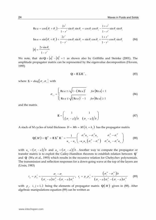
amplitude propagator matrix can be represented by the eigenvalue decomposition (Hovem,
1995)
1Q EΣE , (85)
where 1 2,diag Σ with
2
1,2
2
Re 1 Re Re 1
Re Re 1 Re 1
a i a for a
a a for a
(86)
and the matrix
1 2
1 1
a b a b E (87)
A stack of M cycles of total thickness 1 2
D Mh M h h has the propagator matrix
1 22 2 21 2 11
22 21 21 22 2 1 2 22 1 21
1M M M M
M M
M M M M
u uM
u u u u u u
Q Q EΣ E (88)
with 21 1
u a b and 22 2
u a b . Another way to compute the propagator or
transfer matrix is to exploit the Cailey-Hamilton theorem to establish relation between 2
Q
and Q (Wu et al., 1993) which results in the recursive relation for Chebychev polynomials.
The transmission and reflection responses for a down-going wave at the top of the layers are
(Ursin, 1983)
2 11 12 1
22 12 22
2 2 1 1 2 2 1 1
,
M M
D DM M M M
bt p r p p
a a a a
(89)
with , , 1, 2ij
p i j being the elements of propagator matrix MQ given in (88). After
algebraic manipulations equation (89) can be written as
www.intechopen.com

Acoustic Waves in Layered Media - From Theory to Seismic Applications
25
1
22
2
2
2
Imcos sin
sin sin
sin cos Im sin Im 11 sin 1
sin
sin sin
sin cos Im sin sin 1
i
D
i
D D
aM i M
et
M i a M a CM
b M M Cer t b
M i a M C
, (90)
where and C are the phase and amplitude factors, respectively, and is the phase of
the eigen-value. The equation for transmission response in periodic structure was
apparently first obtained in the quantum mechanics (Cvetich and Picman, 1981) and has
been rediscovered several times. For extensive discussion see reference 13 in Griffiths and
Steinke (2001). The reflection and transmission response satisfy
2 2
1D Dt r , (91)
which is conservation of energy. When Re 1a , the eigen-values give a complex phase-
shift, representing a propagating regime. Then equation (86) gives
1,2
i
e (92)
with cos Re a , which may be obtained from Floquet solution for periodic media, but for
first time appeared in Brekhovskikh (1960), equation (7.25). Then we use
2
cos sincos
sin1
,M M
C b
C
, (93)
in equation (90). Equation (93) for the amplitude factor is given in a form of Chebychev
polynomials of the second kind written in terms of sinusoidal functions. When Re 1a ,
the eigen-values are a damped or increasing exponential function, representing an
attenuating regime. Then equation (86) gives
1,2
e
(94)
with cosh Re a . Then the reflection and transmission responses are still given by
equation (90) but with phase and amplitude factors now given by
2
cosh sinhcos
sinh1
,M M
C b
C
, (95)
For the limiting cases with Re 1a , there is a double root
1 , 2
Re a (96)
www.intechopen.com

Waves in Fluids and Solids
26
and then we must use
2 2
1cos
1
, C b M
b M
(97)
Note, that in this case 2 2
Imb a . To compute expressions (93) and (95) for even number
M we use (Gradshtein and Ryzhik, 1995, equation 1.382)
2
2 22 2
22 21 1
1 1 Re 1 Recos 1 Re 1
2 11 sin sin
2
,
M M
k k
a aC b M a
k kC
M M
(98)
The transmission response from equation (84) can be expressed via the complex phase factor :
i
Dt e
(99)
with
21
ln 12i C . (100)
The angular wavenumber is denoted k . With RekD or cos coskD , the
phase velocity is given by
v k D . (101)
Using notations from Carcione (2001), the dispersion equation can be written as , cos cos 0F k kD , and the expression for group velocity is
F k D
VF
. (102)
7.2 Equivalent time-average and effective medium
The behaviour of the reflection and transmission responses is determined by Re a which is
one for 0f . The boundaries between a propagating and attenuating regime are at
Re 1a (see equation (84)) given by the equation
1 21
tan tan2 2 1
r
r
. (103)
For low frequencies the stack of the layers behaves as an effective medium with a velocity
defined by (Backus, 1962; Hovem, 1995) and can be defined as the zero-frequency limit
( 0EFv v from equation (101))
www.intechopen.com

Acoustic Waves in Layered Media - From Theory to Seismic Applications
27
2
1 2
2 2 2 2
1 2
1 1 4 1
1EF TA
h h r
v v h v v r . (104)
This occurs for frequencies below the first root of the equation Re 1a . For higher
frequencies the stack of the layers is characterized by the time-average velocity defined by
the infinite frequency limit ( TAv v from equation (101))
1 2
1 2 1 2
1 1
TA
h h
v h h v v
. (105)
This occurs for frequencies above the second root of the equation Re 1a . There is a
transition zone between these two roots in which the stack of layers partly blocks the
transmitted wave. The behaviour of the medium is characterized by the ratio between wavelength and layer
thickness. This is given by
1 2
1TAv
h f h h f t
, (106)
where t is the traveltime through the two single layers. To estimate the critical ratio of
wavelength to layer thickness we assume 1 2
2t t t . The effective medium limit the
occurs at
1
1
1tan
1
ra
r
, (107)
and the time-average limit the occurs at
1
2
1tan
2 1
ra
r
, (108)
For small values of 1r we obtain
1
1,2
2tan 4 1
4 2
r ra
. (109)
The transition between an effective medium to time average medium is schematically
illustrated in Figure 12. Since the boundaries for the transmission zone in equation (103) are
periodic functions of frequency, the low wavelength zone (high frequencies) is more
complicated than shown in this figure.
www.intechopen.com

Waves in Fluids and Solids
28
0,0 0,1 0,2 0,3 0,4 0,5 0,6 0,7 0,8 0,9
0
4
8
12
16
20
24
28
32
36
40
/d
Time average medium
Effective medium
Transition zone
Absolute value of r
Fig. 12. Schematic representation of the critical d ratio as function of reflection
coefficient (1 2 ) (Stovas&Ursin, 2007).
7.3 Reflection and transmission responses versus layering and layer contrast
We use a similar model as in Marion and Coudin (1992) with three different reflection
coefficients: the original 0.87r and 0.48r and 0.16r . We use m and Hz instead of
mm and kHz . The total thickness of the layered medium is 51k k
D M h m is constant.
, 1, 2, 4, ..., 64k
M k is the number of cycles in the layered medium, so that the individual layer
thickness is decreasing as k is increasing. The ratio 1 2 1 2 1 2 2 1
0.91t t h v h v . The
other model parameters are given in Stovas and Ursin (2007).
0 100 200 300 400 500 600 700
-1
0
1
Frequency [Hz]
-1
0
1-1
0
1-1
0
1-1
0
1-1
0
1-1
0
1
M1
M2
M4
M8
M16
M32
M64
r=0.16
0 100 200 300 400 500 600 700
-1
0
1
Frequency [Hz]
-1
0
1-1
0
1-1
0
1-1
0
1-1
0
1-1
0
1
M1
M2
M4
M8
M16
M32
M64
r=0.48
0 100 200 300 400 500 600 700
-1
0
1
Frequency [Hz]
-1
0
1-1
0
1-1
0
1-1
0
1-1
0
1-1
0
1
M1
M2
M4
M8
M16
M32
M64
r=0.87
Fig. 13. Re a as function of frequency. Re 1a is only plotted with area filled under the
curve (Stovas&Ursin, 2007).
www.intechopen.com

Acoustic Waves in Layered Media - From Theory to Seismic Applications
29
0 100 200 300 400 500 600 700
-1,0-0,50,00,51,0
Frequency [Hz]
-1,0-0,50,00,51,0
-1,0-0,50,00,51,0
-1,0-0,50,00,51,0
-1,0-0,50,00,51,0
-1,0-0,50,00,51,0
-1,0-0,50,00,51,0
M1
M2
M4
M8
M16
M32
M64
r=0.16
0 100 200 300 400 500 600 700
-1,0-0,50,00,51,0
Frequency [Hz]
-1,0-0,50,00,51,0
-1,0-0,50,00,51,0
-1,0-0,50,00,51,0
-1,0-0,50,00,51,0
-1,0-0,50,00,51,0
-1,0-0,50,00,51,0
M1
M2
M4
M8
M16
M32
M64
r=0.48
0 100 200 300 400 500 600 700
-1,0-0,50,00,51,0
Frequency [Hz]
-1,0-0,50,00,51,0
-1,0-0,50,00,51,0
-1,0-0,50,00,51,0
-1,0-0,50,00,51,0
-1,0-0,50,00,51,0
-1,0-0,50,00,51,0
M1
M2
M4
M8
M16
M32
M64
r=0.87
Fig. 14. The phase function cos as a function of frequency (from equation (98)) shown by
solid line and cos corresponding to the single layer with time-average velocity shown by
dashed line (Stovas&Ursin, 2007).
The very important parameter that controls the regime is Re a (equation (84)). The plots of
Re a versus frequency are given in Figure 13 for different models. One can see that the
propagating and attenuating regimes are periodically repeated in frequency. The higher
reflectivity the more narrow frequency bands are related to propagating regime ( Re 1a ).
One can also follow that the first effective medium zone is widening as the index of model
increases and reflection coefficient decreases, and that the wavelength to layer thickness
ratio is the parameter which controls the regime. The gaps between the propagating
regime bands become larger with increase of reflection coefficient. These gaps correspond to
the blocking or attenuating regime. The graphs for the phase factor cos and amplitude
factor C (equation (98)) are shown in Figure 14 and 15, respectively. The dotted lines in
Figure 14 correspond to the time-average phase behaviour. One can see when the computed
phase becomes detached from the time-average phase. Note also the anomalous phase
behaviour in transition zones. The amplitude factor C (Figure 15) has periodic structure,
and periodicity increase with increase of reflection coefficient. In transition zones the
amplitude factor reaches extremely large values which correspond to strong dampening.
The transmission and reflection amplitudes are shown in Figure 16. The larger reflection
coefficient the more frequently amplitudes change with frequency. The transition zones can
be seen by attenuated values for transmission amplitudes. With increase of reflection
www.intechopen.com

Waves in Fluids and Solids
30
0 100 200 300 400 500 600 700
-2-1012
Frequency [Hz]
-2-1012
-2-1012
-2-1012
-2-1012
-2-1012
-2-1012
M1
M2
M4
M8
M16
M32
M64
r=0.16
0 100 200 300 400 500 600 700
-10-505
10
Frequency [Hz]
-10-505
10-10
-505
10-10
-505
10-10
-505
10-10
-505
10-10
-505
10
M1
M2
M4
M8
M16
M32
M64
r=0.48
0 100 200 300 400 500 600 700
-20-10
01020
Frequency [Hz]
-20-10
01020
-20-10
01020
-20-10
01020
-20-10
01020
-20-10
01020
-20-10
01020
M1
M2
M4
M8
M16
M32
M64
r=0.87
Fig. 15. The amplitude function C (from equation (98)) as a function of frequency (very
large values of C are not shown) (Stovas&Ursin, 2007).
coefficient the dampening in transmission amplitudes becomes more dramatic. The exact
transmission and reflection responses are computed using a layer recursive algorithm (Ursin
and Stovas, 2002). We use a Ricker wavelet with a central frequency of 500 Hz. The
transmission and reflection responses are shown in Figure 17 and 18, respectively. No
amplitude scaling was used. One can see that these plots are strongly related to the
behaviour of Re a (Figure 13). The upper seismogram in Figure 17 is similar to the Marion
and Coudin (1992) experiment and the Hovem (1995) simulations. The effects related to the
effective medium (difference between the first arrival traveltime for model 1
M and 64
M and
the transition between effective and time average medium, models 4 16
M M ) are the more
pronounced for the high reflectivity model. For this model the first two traces (models 1
M
and 2
M ) are composed of separate events, and then the events become more and more
interferential as the thickness of the layers decrease. Model 8
M gives trains of nearly
sinusoidal waves (tuning effect). The transmission response for model 16
M is strongly
attenuated, and models 32
M and 64
M behave as the effective medium. From Figures 13-16
and the transmission and reflection responses (Figures 17 and 18) one can distinguish
between time average, effective medium and transition behaviour. This behaviour can be
seen for any reflectivity, but a decrease in the reflection coefficient results in the convergence
of the traveltimes for time-average and effective medium. This makes the effective medium
arrival very close to the time average one. Note also that for the very much-pronounced
www.intechopen.com

Acoustic Waves in Layered Media - From Theory to Seismic Applications
31
0 100 200 300 400 500 600 700
0,00,51,0
M64
M32
M16
M8
M4
M2
M1
r=0.16
Frequency [Hz]
0,00,51,0
0,00,51,0
0,00,51,0
0,00,51,0
0,00,51,0
0,00,51,0
0 100 200 300 400 500 600 700
0,00,51,0
M64
M32
M16
M8
M4
M2
M1
r=0.48
Frequency [Hz]
0,00,51,0
0,00,51,0
0,00,51,0
0,00,51,0
0,00,51,0
0,00,51,0
0 100 200 300 400 500 600 700
0,00,51,0
M64
M32
M16
M8
M4
M2
M1
r=0.87
Frequency [Hz]
0,00,51,0
0,00,51,0
0,00,51,0
0,00,51,0
0,00,51,0
0,00,51,0
Fig. 16. The transmission amplitude (solid line) and reflection amplitude (dotted line) as function of frequency (Stovas&Ursin, 2007).
0,00 0,02 0,04 0,06 0,08 0,10
-404
M4
M2
M1
r=0.16
Time [s]
-404
-404
-404
M64
M32
M16
M8
-404
-404
-404
0,00 0,02 0,04 0,06 0,08 0,10
-3,50,03,5
M4
M2
M1
r=0.48
Time [s]
-3,50,03,5
-3,50,03,5
-3,50,03,5
M64
M32
M16
M8
-3,50,03,5
-3,50,03,5
-3,50,03,5
0,00 0,02 0,04 0,06 0,08 0,10
-101
M4
M2
M1
r=0.87
Time [s]
-101
-101
-101
M64
M32
M16
M8
-101
-101
-101
Fig. 17. Numerical simulations of the transmission response (Stovas&Ursin, 2007).
www.intechopen.com

Waves in Fluids and Solids
32
0,00 0,02 0,04 0,06 0,08 0,10
-1,50,01,5
Time [s]
-1,50,01,5
M1
M2
M4
M8
M16
M32
M64
-1,50,01,5
-1,50,01,5
-1,50,01,5
-1,50,01,5
-1,50,01,5
r=0.16
0,00 0,02 0,04 0,06 0,08 0,10
-303
Time [s]
-303
M1
M2
M4
M8
M16
M32
M64
-303
-303
-303
-303
-303
r=0.48
0,00 0,02 0,04 0,06 0,08 0,10
-404
Time [s]
-404
M1
M2
M4
M8
M16
M32
M64
-404
-404
-404
-404
-404
r=0.87
Fig. 18. Numerical simulations of the reflection response (Stovas&Ursin, 2007).
effective medium (model 64
M , 0.87r ) one can see the effective medium multiple on the
time about 0.085s. The reflection responses (Figure 18) demonstrate the same features as the
transmission responses (for example strongly attenuated transmission response is related to
weak attenuated reflection response). Effective medium is represented by the reflections
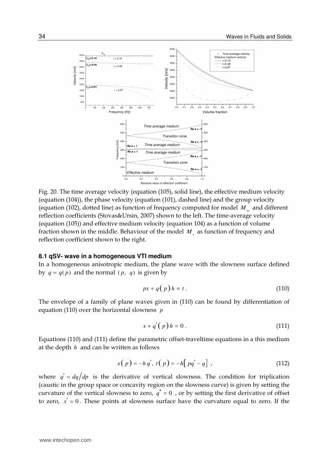
from the bottom of the total stack of the layers. The phase velocities are computed from the
phase factor (equation (100)) and shown in Figure 19 as a function of frequency. The phase
velocity curve starts from the effective medium velocity and at the critical frequency it
jumps up to the time-average velocity. One can see that the width of the transition zone is
larger for larger values of reflection coefficient. The difference between the effective medium
velocity and time-average velocity limits also increases with reflection coefficient increase.
In Figure 20, one can see time-average velocity, effective medium velocity, phase velocity
(equation (100)) and group velocity (equation (102)) computed for reflection coefficients 0.16,
0.48 and 0,87 and model 64
M . In this case we are in the effective medium zone. The larger
reflection coefficient is, the lower effective medium velocity, the larger difference between
the phase and group velocity and the velocity dispersion becomes more pronounced. The
effective medium velocity limit also depends on the volume fraction ( 2 1 2
h h h ) for
one cycle (see equation (104)). This dependence is illustrated in Figure 21 for different values
of reflection coefficient. The maximum difference between the time-average and effective
medium velocity reaches 2.191 km/s at 0.18 ( 0.87r ), 0.513 km/s at 0.24 ( 0.48r )
and 0.053 km/s at 0.26 ( 0.16r ). One can see that for the small values of reflection
coefficient the difference between the time-average velocity (high-frequency limit) and
effective medium velocity (low frequency limit) becomes very small. For large values of
reflection coefficient and certain range of volume fraction the effective medium velocity is
www.intechopen.com
Acoustic Waves in Layered Media - From Theory to Seismic Applications
33
0 100 200 300 400 500 600 700
3600
3800
4000
4200
M64
M32
M16
M8
M4
M2
M1
VEF
VTA
r=0.16
Frequency [Hz]
0 100 200 300 400 500 600 700
2800
3200
3600
4000
4400
4800
M64
M32
M16
M8M4
M2
M1
VEF
VTA
r=0.48
Frequency [Hz]
0 100 200 300 400 500 600 700
1500
3000
4500
6000
M64
M32
M16
M8M4
M2
M1
VEF
VTA
r=0.87
Frequency [Hz]
Fig. 19. The phase velocity (equation (101)) in m/s as function of frequency (Stovas&Ursin, 2007).
smaller than the minimum velocity of single layer constitutes. The effective medium is related
to the propagating regime. The effective medium velocity depends on the reflection coefficient.
The lesser contrast the higher effective medium velocity (the more close to the time-average
velocity). One can also distinguish between effective medium, transition and time average
frequency bands (Figure 22). These bands are separated by the frequencies given by conditions
from the first two roots of equation Re 1a . The first root (equation (107)) gives the limiting
frequency for effective medium. The second one (equation (108)) gives the limiting frequency
for time average medium. From Figure 22, one can see that the transition zone converges to the
limit 4 with decreasing reflection coefficient. The first transition zone results in the most
significant changes in the phase velocity and the amplitude factor C .
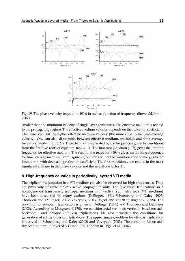
8. High-frequency caustics in periodically layered VTI media
The triplications (caustics) in a VTI medium can also be observed for high-frequencies. They are physically possible for qSV-wave propagation only. The qSV-wave triplications in a homogeneous transversely isotropic medium with vertical symmetry axis (VTI medium) have been discussed by many authors (Dellinger, 1991; Schoenberg and Daley, 2003; Thomsen and Dellinger, 2003; Vavrycuk, 2003; Tygel and et. 2007; Roganov, 2008). The condition for incipient triplication is given in Dellinger (1991) and Thomsen and Dellinger (2003). According to Musgrave (1970), we consider axial (on- axis vertical), basal (on-axis horizontal) and oblique (off-axis) triplications. He also provided the conditions for generation of all the types of triplications. The approximate condition for off-axis triplication is derived in Schoenberg and Daley (2003) and Vavrycuk (2003). The condition for on-axis triplication in multi-layered VTI medium is shown in Tygel et al. (2007).
www.intechopen.com
Waves in Fluids and Solids
34
0 100 200 300 400 500 600 700
800
1200
1600
2000
2400
2800
3200
3600
4000V
TA
VEF
(r=0.87)
VEF
(r=0.48)
VEF
(r=0.16) r = 0.16
r = 0.48
r = 0.87
Ve
locity [
m/s
]
Frequency [Hz]
0,0 0,1 0,2 0,3 0,4 0,5 0,6 0,7 0,8 0,9 1,0
2000
2500
3000
3500
4000
4500
5000
5500
Ve
locity [
m/s
]
Volume fraction
Time-average velocity
Effective medium velocity
r=0.16
r=0.48
r=0.87
0,0 0,2 0,4 0,6 0,8 1,0
0
100
200
300
400
500
600
0
100
200
300
400
500
600Time average medium
Time average medium
Time average medium
Transition zone
Transition zone
Effective medium
Re a = -1
Re a = -1
Re a = 1
Re a = -1
Re a = 1
Re a = -1
Fre
qu
en
cy [H
z]
Absolute value of reflection coefficient
Fig. 20. The time average velocity (equation (105), solid line), the effective medium velocity
(equation (104)), the phase velocity (equation (101), dashed line) and the group velocity
(equation (102), dotted line) as function of frequency computed for model 64
M and different
reflection coefficients (Stovas&Ursin, 2007) shown to the left. The time-average velocity
(equation (105)) and effective medium velocity (equation 104) as a function of volume
fraction shown in the middle. Behaviour of the model 4
M as function of frequency and
reflection coefficient shown to the right.
8.1 qSV- wave in a homogeneous VTI medium
In a homogeneous anisotropic medium, the plane wave with the slowness surface defined
by ( )q q p and the normal ( , )p q is given by
px q p h t . (110)
The envelope of a family of plane waves given in (110) can be found by differentiation of
equation (110) over the horizontal slowness p
0x q p h . (111)
Equations (110) and (111) define the parametric offset-traveltime equations in a this medium
at the depth h and can be written as follows
,x p h q t p h pq q , (112)
where q dq dp is the derivative of vertical slowness. The condition for triplication
(caustic in the group space or concavity region on the slowness curve) is given by setting the
curvature of the vertical slowness to zero, 0q , or by setting the first derivative of offset
to zero, 0x . These points at slowness surface have the curvature equal to zero. If the
www.intechopen.com

Acoustic Waves in Layered Media - From Theory to Seismic Applications
35
triplication region is degenerated to a single point, it is called incipient triplication. At that
point we have 0q and 0q . For the incipient horizontal on-axis triplication, it is not
true, because at that point q equal to infinity, and we have to take the corresponding limit.
The triplications can be also related to the parabolic points on the slowness surface with one
of the principal curvatures being zero. The exception is the incipient vertical on-axis
triplication with both principal curvatures equal to zero. The phase velocity can be written
(Schoenberg and Daley, 2003) as a function of phase angle
2
2 0
2
Sv
v fg
, (113)
where 0 Sv is the vertical S-wave velocity, and function f is defined as
2 2
1 1 1P S
f f eu g eu g E u , (114)
where + and – correspond to qP- and qSV-wave, respectively, cos 2u , and parameters
11 33
11 33
c ce
c c
, 55
11 33
2cg
c c and
2
11 55 33 55 13 55
2
11 33
4( )( ) 4( )
( )
c c c c c cE
c c
, which can be written
in terms of Thomsen (1986) anisotropy parameters
2
01 1 2 1 1, ,e g E e e g (115)
and 0 0 0S P
v v is the S- to P-wave vertical velocity ratio. Note, that 0 1g and
1e g . Parameter E is also known as anelliptic parameter (Schoenberg and Daley,
2003) since it is proportional to the parameter , 2
02 1E g e g ,
which is responsible for the anellipticity of the slowness surface and for the non-
hyperbolicity of the traveltime equation. Vavrycuk (2003) used parameter to estimate the
critical strength of anisotropy for the off-axis triplications in a homogeneous VTI medium.
For the waves propagating for entire range of the phase angles, it is required that the
function ( , )Sf u E and the expression under the square-root in equation (114)
2 2
( , ) (1 ) (1 )s u E eu g E u (116)
should be non-negative for all | | 1u . Solving equations ( , ) 0Sf u E and ( , ) 0s u E for
the parameter E , results in the following explicit functions 2
4 (1 )( )
1f
g euE u
u
and
2
2
(1 )( )
1s
eu gE u
u
, where the sub-indices f and s indicate the solutions for the
equations 0f and 0s , respectively. Function ( )f
E u defines the minimum plausible
values for the parameter E in order to satisfy the condition 2
0v , while the function
( )s
E u defines the maximum plausible values for the parameter E in order to satisfy the
condition 2
Im 0v . By setting derivatives 0f
dE du and 0s
dE du , we obtain that,
www.intechopen.com

Waves in Fluids and Solids
36
for the range 1u , implicit functions ( , ) 0Sf u E and ( , ) 0s u E have the maximum and
the minimum at the points 1
A (from 0f and 0f
dE du ) and 2
A (from 0s and
0s
dE du ), respectively (Figure 21). The coordinates for these points are
2 2 2 2
1 1 2 2(1 1 ) / , 2 (1 1 ), /(1 ), (1 )
A A A Au e e E g e u e g E g e . (117)
Fig. 21. Schematic plot of the triplication conditions on ,u E space. The graphs for
( , ) 0Sf u E and ( , ) 0s u E are shown by dash line, and the graph for ( , ) 0
Su E is
shown by solid line. Points 1
A and 2
A correspond to the extrema of the functions
( , ) 0Sf u E and ( , ) 0s u E , respectively. Points
1B and
2B are the limiting points on the
lower branch of ( , ) 0Su E from the left and from right, respectively. Points
2A ,
1C and
2C correspond to the extrema of the function ( , ) 0
Su E which has two branches limiting
the triplication areas: 1 – vertical on-axis, 2 – horizontal on-axis and 3 – off-axis. The
condition 1 2A A
E E E is a necessary and sufficient condition for existence of qP- and qSV-
waves for entire range of the phase angles (Roganov&Stovas, 2010).
Therefore, the parameter E is limited as follows 1 2A A
E E E . Note, that 1
0A
u if 0e .
The equation for 2A
u was shown in Schoenberg and Daley (2003). The lower limit yields the
condition 2
0v , while the upper limit is related to the Thomsen’s (1986) definition of
parameter , i.e. 2
01 2 0 . The range for parameter E yields a necessary and
sufficient condition for the Christoffel matrix being positive definite for the entire range of
the phase angles. Therefore, this condition is valid for all physically plausible medium
parameters. Using equation (113) and
sin ( ) , cos ( ) , cos 2p V q V u ,
we obtain that for both types of waves we have the following equalities p
0 0
1 (1 ) 1 (1 ),
S S
u g u gp q
v f v f
, (118)
where P Sf f depending on the wave-mode (see equation (114)). The first and second
derivatives of the vertical slowness are given by
www.intechopen.com

Acoustic Waves in Layered Media - From Theory to Seismic Applications
37
/
/
( (1 ))
( (1 ))
u
u
dq p f f u
dp q f f u
, (119)
2
2 2 3 3
0
2
S
d q g
dp v q
, (120)
where /
uf df du and
1 1 1 1 ,P S P S
e g eu g E u e g s m n s (121)
with s given in equation (116) and
2 32 2 3 2 2 2 2 2 2
2 22 2 2 2 2 2 2 2
2 2 2 3 1 3 1 1 1 2 2 1 1
1 1 6 4 1 1 2 1 1
m E e e g g u e g u e g u g g e g e g eu g
n u E e g g u e g u e g E g e eu g
. (122)
For qSV and qP waves propagating in a homogeneous VTI medium, the triplication
condition is given by (Roganov, 2008)
( , ) 0Su E , (123)
( , ) 0Pu E . (124)
Equations (121)-(122) are too complicated to define the influence of parameters e and g on
the form of the curves given by equations (123) and (124). Nevertheless, these equations can be
used for numerical estimation of the position for triplications with any given values for e and
g , as well as for the following theoretical analysis. It is well known that qP waves never have
triplications in a homogeneous VTI medium (Musgrave, 1970; Dellinger, 1991; Vavrycuk,
2003), and, therefore, the equation (124) has no roots for propagating qP waves. By taking all
the physically possible values for u , e , g and E , one can prove that if ( , ) 0s u E , 1u ,
0 1g and 1e g , the following inequality always takes place, ( , ) 0Pu E .
The product of ( , )Pu E and ( , )
Su E
2 2
( , ) ( , ) ( , )P S
u E u E u E m sn (125)
given by polynomial with the sixth order in u and fifth order in E , can also be used to
define the triplications for qSV-waves. For elliptical anisotropy, 0E , we have the
equalities ( , ) 2Sf u E g and
2
55( )V c . In this case, both the slowness and the group
velocity surfaces are circles, and qSV-waves have no triplications. The straight line given by
0E , separate the plane ( , )u E into sub-planes with non-crossing branches of the curve
( , ) 0Su E . One of these branches is located in the range of values
10
AE E and 1u
and is limited from the left and the right by the points 1
B and 2
B , respectively. The
coordinates of these points are (Figure 23)
www.intechopen.com

Waves in Fluids and Solids
38
1 1 2 2
1, 1 1, 1,B B B B
u E g e g u E g e g , (126)
while the second branch is closed and located in the range of values 2
0A
E E . The
limited values 1
0B
E and 2
0B
E , that follows from inequalities 0 1g and 1e g .
Under the lower branch of the curve ( , ) 0Su E on the plane ( , )u E , there are two
parameter areas resulting in the on-axis triplications (both for vertical and horizontal axis),
while the upper branch of the curve ( , ) 0Su E defines the parameter area for the off-axis
triplications. In Figure 23, these areas are denoted by numbers 1, 2 and 3, respectively.
Therefore, the on-axis triplications can simultaneously happen for both axis, if 0E , while
the off-axis triplications can exist only alone, if 0E . Let us define the critical values for
parameter E in ( , )u E space with horizontal tangent line (1A
E , 2A
E , 1C
E and 2C
E in Figure
23) that define the incipient triplications. In order to do so we need to solve the system of
equations
( , ) 0
( , )0
S
S
u E
u E
u
. (127)
For the range of parameters 1 2A A
E E E and 1u , system of equations (127) has four
solutions, where the first two solutions 1 1,
A Au E and
2 2,
A Au E are defined above. For
the second two solutions 1 1,
C Cu E and
2 2,
C Cu E we have
1 2 2C C Au u u , while
1CE and
2CE are the largest (always positive) and intermediate (always negative) roots of the cubic
equation
23 2 2 2 2 2 2 2 2
3 3 2 3 8 1 16 1 1 0t E E g e g E g g e E g e g e . (128)
Equations similar to our equation (128) are derived in (Peyton, 1983; Schoenberg and Helbig,
1997; Thomsen and Dellinger, 2003; Vavrycuk, 2003; Roganov, 2008). To prove that equation
( ) 0t E gives the positions for the critical points of the curve ( , ) 0u E one can
substitute 2A
u u . Consequently, we have
2 2
2
2 22
1( , ) ( ) ( , )
1A A
g eu E t E p u E
g (129)
and
2
22 2
( , ) 6 (1 )( , )
(1 )
A
A
u E e gu E
u g e
. (130)
Therefore, if ( ) 0t E and 2A
u u , then system of equations (127) is obeyed. The least root
of equation (128) is located in the area defined by 1E and holds also equation
( , ) 0Pu E . It is located outside the region
1 2A AE E E and does not define any qSV
wave triplication. The intermediate root defines the critical point 2
C on the lower branch of
the curve (123). The minimum point 1
A (dividing the triplication domain 1 and 2) is also
www.intechopen.com

Acoustic Waves in Layered Media - From Theory to Seismic Applications
39
located on the same branch. The largest root corresponds to the minimum point 1
C on the
upper branch of the curve (123). If 1 1C A
E E E , we have off-axis triplications. The
coordinates 1C
E and 2C
E are given by equations
1 2
2 sin 2 / 3 / 6 , 2 sin 2 / 3 5 / 6C C
E Q d E Q d , (131)
where
2 2 2 2
2 2 2 2
3 / 2
[(1 ) ](1 )1 2 / 3 1 2 / 3 arccos, ,
g e e gd g g e Q e g g
Q . (132)
The case for the qSV-wave vertical on-axis incipient triplication can be obtained by setting
1u ( 0 ) with condition (120) being simplified to 2B
E E or 0.5 or 2
0nmov
(Tygel et al., 2007). The case for the qSV-wave horizontal on-axis incipient triplication can be
obtained by setting 1u ( 2 ) with condition (118) being simplified to 1B
E E or 2 2
0 01 2 2 1 . If
1 1 2min( , )
A B BE E E E , we have both on-axis triplications.
If 0e (or 0 ), then we have the following equality 1 2B B
E E , and, therefore, both on-
axis triplications are incipient.
8.2 Extension of qSV-wave triplications for multilayered case
From the ray theory it follows that for any vertically heterogeneous medium including
horizontally layered medium, kinematically effective vertical slowness is always the average
of the vertical slownesses from the individual layers. We have to stress that our approach is
based on the high-frequency limit of the wave propagation, not on the low-frequency one
which results in effective medium averaging. Since the wave propagates through the
layered medium with the same horizontal slowness p , the effective vertical slowness has
very simple form
q q , (133)
where denotes the arithmetic thickness averaging, i i i
m m h h , with
, 1,ih i N being the thickness of layer i in the stack of N layers. With notation (133),
equations (112) are valid for the multilayered case. Similar approach is used in Stovas (2009)
for a vertically heterogeneous isotropic medium. If a layered VTI medium results in more
then one caustic, there is no any kinematically effective VTI medium given in equation (133),
which can reproduce the same number of caustics. This statement follows from the fact that
a homogeneous VTI medium might have only one off-axis triplication. Therefore, the second
derivative of the effective vertical slowness is given by
2
2 2 3 3
0
2
S
d q g
dp v q
. (134)
With equation (134) the condition for off-axis, vertical on-axis and horizontal on-axis
triplications in multi-layered VTI medium takes the form (Roganov and Stovas, 2010)
www.intechopen.com

Waves in Fluids and Solids
40
2 3 3
0
0S
S S S
g
v q
. (135)
To obtain the condition for incipient vertical triplications, we have to substitute 1u и
0p into equation (135). After some algebraic manipulations, we obtain
2
0 2
2
1, 0 2
( )0
S B
u p B
d q v E E
dp E
. (136)
Similar equation can be derived by using the traveltime parameters. Tygel et al. (2007)
shown that the vertical on-axis triplications in the multilayered VTI medium are defined by
the normal moveout velocity (representing the curvature of the traveltime curve t x taken
at zero offset): 2
0nmov , where
2 2 1 1
0 0nmo nmo S Sv v v v
is the overall normal moveout velocity
squared. In order to use equation (135), the function u p has to be defined in terms of
horizontal slowness for each layer
2 2
0 S
S
a p v bu p u p
c
, (137)
where
2 2 2 4 4
0 0
22 2 2 2 2 2 4 4
0 0
2 2 2 4 4
0 0
1 2
1 2 2 1 1 4 4
2
S S
S S
S S
a g g e g p v egp v
b g e g g eg e g e g E p v E Eg e g p v
c g egp v Ep v
. (138)
Function 0b p if 0E . We are going to prove that the function b b p from
equation (138) is positive for all physically plausible parameters e and g , if anelliptic
parameter 0E . Solving bi-quadratic equation 0b p yields
22 2
1, 2 ,3 , 4 2 2 2
0 ,
1 2 1 2 1 11
4 4S
Eg e g eg e g E e e E g
pv E Eg e g
(139)
The expression under the inner square root in equation (139) can be written as
22 2 2
0 01 4 1 1 2e E g (140)
Note, that 2
01 2 0 (it follows from Thomsen’s (1986) definition of parameter ).
Taking into account that 1e , and 22
0 1 0b p g e g and 2 2
01 1 1 0
Sb p v e e g , one can see that if 0E , the expression under the
square root in equation (139) is negative, and the equation 0b p has no roots. Function c c p can take zero value at
www.intechopen.com

Acoustic Waves in Layered Media - From Theory to Seismic Applications
41
2
0
1
S
gp p e e E
v E (141)
To compute u u p from equation (137) we need to take the limit given by
2 2 2 2
3 2 2 2 2
4 2 4 1Lim
4 3 4 1p p
e g E e e g eg E e E eg E e gu p u p
e g E e e eg E e E e g E e g
. (141)
If 0c p , that happens at
2
0
1
S
gp p e e E
v E , (142)
function u p takes the value
2 2 2 2
3 2 2 2 2
4 2 4 1
4 3 4 1
e g E e e g eg E e E eg E e gu p
e g E e e eg E e E e g E e g
. (143)
Note that in the presence of on-axis triplication (for the horizontal axis), function ( )u p has
two branches when 0
1S
p v , and the second branch is defined by
2 2
0P Su p u p a p v b c . The incipient off-axis triplication condition in a multi-
layered medium is given by equation (Roganov and Stovas, 2010)
3 3
0
0
S
S S
S
dg q
v dp
. (144)
Functions Sq and
S ,
S defined in equations (118) and (121), respectively, are given in
terms of u . To compute the derivatives in equation above one need to exploit equation (117)
for u u p and apply the chain rule, i.e. S S
dq dp dq du du dp . For a given model this
equation can be resolved for horizontal slowness and used to estimate the limits for the
vertical slowness approximation or traveltime approximation. For multilayered case, the
parametric offset-traveltime equations (112) take the following form
,x p H q t p H pq q , (145)
where i
H h is the total thickness of the stack of layers.
www.intechopen.com

Waves in Fluids and Solids
42
8.3 Converted wave case
In the special case of converted qP-qSV waves (C-waves) in a homogeneous VTI medium, the condition (113) reduces to
3 3 3 3
0S P
S S P Pq q
. (146)
To compute functions P
, P
q and P
we need to define P
u p which can be computed
similar to equation (117)
2 2
0 S
P
a p v bu p
c
, (147)
where functions a , b and c can be computed from equation (138). One can show that for
the range of horizontal slowness corresponding to propagating qP-wave, the sum
3 3 3 3
0S P
S S P Pq q
, (148)
which means that the converted qP-qSV waves in a homogeneous VTI medium have no
triplications. In Figure 22 one can see the functions 3 3
2S S S
q (controlling the triplications
for qSV-wave), 3 3
2P P P
q (controlling the triplications for qP-wave) and 3 3 3 3
S S S P P Pq q
(controlling the triplications for converted waves). The model parameters are taken from the
case 1 model 1. One can see that the only function crossing the u axis is the qSV-wave
related one.
-1,0 -0,5 0,0 0,5 1,0
-40
-30
-20
-10
0
10
20
30
S/q
S
3S
3 +
P/q
P
3P
3
2P/q
P
3P
3
2S/q
S
3S
3
u
Fig. 22. The functions controlled the qP- (red line), qSV- (blue line) and qPqSV-wave (black line) triplications. The data are taken from the case 1 model 1 (Roganov&Stovas, 2010).
8.4 Single-layer caustics versus multi-layer caustics
For our numerical tests we consider the off-axis triplications only, because the vertical on-axis triplications were discussed in details in Tygel et. al (2007), while the horizontal on-axis triplications have only theoretical implications.
First we illustrate the transition from the vertical on-axis triplication to the off-axis
triplication by changing the values for parameter E only, 0.3, 0.2, ..., 0.5E . Since the
other parameters remain constant, this change corresponds to the changing in Thomsen’s
www.intechopen.com

Acoustic Waves in Layered Media - From Theory to Seismic Applications
43
(1986) parameter . The slowness surfaces, the curvature of the slowness surfaces and the
traveltime curves are shown in Figure 23. One can see how the anomaly in the curvature
moves from zero slowness to non-zero one.
0,0 0,1 0,2 0,3 0,4 0,5 0,6
0,0
0,1
0,2
0,3
0,4
0,5
0,6
E increase
qs,
s/k
m
Horizontal slowness, s/km
0,0 0,1 0,2 0,3 0,4 0,5
-8
-6
-4
-2
0
2
4
6
8
E increase
-d2q
s /d
p2,
s/k
m2
Horizontal slowness, s/km
0,0 0,5 1,0 1,5 2,0 2,5 3,0 3,5 4,0
0,8
0,9
1,0
1,1
1,2
1,3
1,4
1,5
E increaseTra
ve
ltim
e,
s
Offset, km
Fig. 23. The slowness surface (to the left), the curvature of slowness surface (in the middle)
and the traveltime versus offset (to the right) from the homogeneous VTI media with change
in parameter E only. The model parameters are taken from the model 1 in Table 1.
Parameter E takes the values -0.3, -0.2,…, 0.5. The curves with positive and negative values
for E are shown with red lines and blue lines, respectively. The elliptically isotropic case,
0E , is shown by black line (Roganov&Stovas, 2010).
Next we test the qSV-wave slowness-surface approximations from Stovas and Roganov (2009). The slowness-surface approximations for qSV waves (similar to acoustic approximation for qP waves) are used for processing (in particular, phase-shift migration) and modeling purpose with reduced number of medium parameters. With that respect, it is important to know how the slowness-surface approximations reproduce the triplications. We notice that if the triplication is located for short offset, it can partly be shown up by approximation 1 (short spread approximation). The wide-angle approximations 2 and 3 can not treat the triplications. In the numerical examples provided in Roganov and Stovas (2010), we considered four cases with two layer models when each layer has parameters resulting in triplication for qSV-wave. With changing the fraction ratio from 0 to 1 with the step of 0.1, we can see the transition between two different triplications for cases 1-4. For given numbers of the fraction ratio we can observe the different cases for two-layer triplications. For the overall propagation we can have no triplication (case 1), one triplication (case 2), two triplications (case 3) and one ”pentaplication” or two overlapped triplications (case 4). Intuitively, we can say that the most complicated caustic from N VTI layers can be composed from N
www.intechopen.com

Waves in Fluids and Solids
44
overlapped triplications or one “(2N+1)-plication”. The examples shown in Roganov and Stovas (2010) provide the complete set of situations for off-axis triplications in two-layer VTI media and give a clue what we can expect to see from multilayered VTI media.
9. Phase velocity approximation in finely layered sediments
The effect of multiple scattering in finely layered sediments is of importance for stratigraphic interpretation, matching of well log-data with seismic data and seismic modelling. This problem was first studied in the now classical paper by O'Doherty and Anstey (1971) and further investigated by Shapiro and Treitel (1997). In this paper I derive a new approximation for the phase velocity in an effective medium which depends on three parameters only and show how it depends on the strength of the reflection coefficients (Stovas, 2007). Approximation is tested on the real well log data example and shows very good performance.
9.1 Vertical propagation through the stack of the layers
The transmission and reflection responses of normal-incident plane wave from the stack of N layers are given by the following expressions (Stovas and Arntsen, 2006)
22
11
...1
1 1,
N jNN
D D
NN
iii
jk
N N jk
e r ee r
t r
, (149)
where kr are reflection coefficients, the cumulated phases
1 1
N N
i i i i
i i
h V
, with j
h
and j
V are thickness and velocity in the layer j, respectively, and the reflection coefficient
correlation function
1
2
1 1
...j k
N N
i
k j
k j k
r r e
(150)
The exponential factors in denominators for transmission and reflection response are the phase
delays for direct wave, the product function in transmission response gives the direct
transmission loss and the sum function in reflection response corresponds to contributions
from the primary reflections (first order term) and interbedded multiples (higher order terms).
The phase velocity is given by
1
1 1
1
1 1
sin 2 ...1 1 1 Im 1 1
tan tan1 Re
1 cos 2 ...
N N
k j j k
k j k
N N
TA TA
k j j k
k j k
r r
a aV V D V D
r r
, (151)
where D is the total thickness of the stack and TA N
V D is time-average velocity. The
velocity in zero-frequency limit is given by (Stovas and Arntsen, 2006)
www.intechopen.com
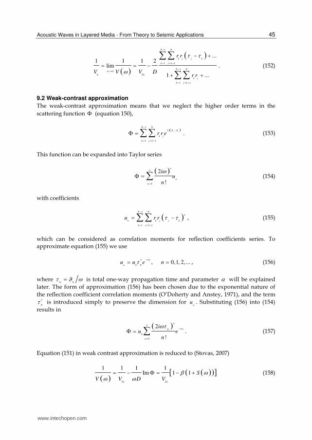
Acoustic Waves in Layered Media - From Theory to Seismic Applications
45
1
1 1
10
0
1 1
...1 1 1 2
lim
1 ...
N N
k j j k
k j k
N N
TA
k j
k j k
r r
V V V Dr r
. (152)
9.2 Weak-contrast approximation
The weak-contrast approximation means that we neglect the higher order terms in the
scattering function (equation 150),
1
2
1 1
j k
N N
i
k j
k j k
r r e
. (153)
This function can be expanded into Taylor series
0
2
!
n
n
n
iu
n
(154)
with coefficients
1
1 1
N N
n
n k j j k
k j k
u r r
, (155)
which can be considered as correlation moments for reflection coefficients series. To approximate equation (155) we use
0
, 0,1, 2, ...n n
n Nu u e n
, (156)
where N N
is total one-way propagation time and parameter will be explained
later. The form of approximation (156) has been chosen due to the exponential nature of
the reflection coefficient correlation moments (O’Doherty and Anstey, 1971), and the term n
N is introduced simply to preserve the dimension for
nu . Substituting (156) into (154)
results in
0
0
2
!
n
nN
n
iu e
n
. (157)
Equation (151) in weak contrast approximation is reduced to (Stovas, 2007)
1 1 1 1Im 1 1
TA TA
SV V D V
(158)
www.intechopen.com

Waves in Fluids and Solids
46
with 0 1
2 2N
u e u and
2
2
1
1 2
2 1 !
n n
nN
n
S en
, where 0
u being considered
as the zero-order auto-correlation moment for reflection coefficients series 1
0
1 1
N N
k j
k j k
u r r
and is the parameter in correlation moments approximation. For practical
use we need the limited number of terms M in equation (160). The zero-frequency limit from
equation (152) is given by 1 1
0 12 1
TA TAV V u D V .
Substituting this limit into equation (158) we obtain
0
1 11
1S
V V
. (163)
Parameter 0 , therefore, describes the relation between two limits 0
1TA
V V and
function S can be interpreted as the normalized relative change in the phase slowness 1 1 1 1
0 0 TAS V V V V .
The phase velocity approximation is described by three parameters only: one-way
propagation time N
; 2) parameter which is ratio of low and high frequency velocity
limits; 3) parameter which describes the structure of the stack.
4200 4220 4240 4260 4280 4300 4320
2500
3000
3500
4000
4500
5000
VP
Depth, m
4200 4220 4240 4260 4280 4300 4320
1,8
1,9
2,0
2,1
2,2
2,3
2,4
2,5
2,6
2,7
4200 4220 4240 4260 4280 4300 4320
-0,08
-0,06
-0,04
-0,02
0,00
0,02
0,04
0,06
0,08
r
0 2 4 6 8 10
-45
-40
-35
-30
-25
-20
-15
-10
-5
ln(-un)=-6.18045-3.46737*n
ln(-
un )
n
0 5 10 15 20 25 30 35 40 45 50
4310
4315
4320
4325
4330
M=11 M=15
M=7
M=3
Ph
as
e v
elo
cit
y, m
/s
Frequency, Hz
Exact
Limited series of S()
Fig. 24. Elastic parameters and reflection coefficients for Tilje formation (to the left), the correlation moments approximation (in the middle) and the phase velocity and its approximations computed from limited series of S . (Stovas, 2007).
For numerical application we use 140m of the real well-log data sampled in 0.125m (Figure
24). This interval related to the Tilje formation from the North Sea. In Figure 24, we also
show how to compute parameters for approximation (156). The one way traveltime is
www.intechopen.com

Acoustic Waves in Layered Media - From Theory to Seismic Applications
47
0.0323N
s , 0.04 and 0.03468 . In particular it means that the time-average
velocity is only 4% higher than the zero frequency limit. The results of using this
approximation with the limited number of terms (M = 3, 7, 11 and 15) in equation (157) are
shown in Figure 24. The exact phase velocity function is obtained from the transmission
response computed by the matrix propagator method (Stovas and Arntsen, 2006). One can
see that with increase of M the quality of approximation increases with frequency.
10. Estimation of fuid saturation in finely layered reservoir
The theory of reflection and transmission response from a stack of periodically layered sediments can be used for inversion of seismic data in turbidite reservoirs. In this case, the model consists of sand and shale layers with quasi-periodical structure. The key parameters we invert for are the net-to-gross ratio (the fractural amount of sand) and the fluid saturation in sand. The seismic data are decomposed into the AVO (amplitude versus offset) or AVA (amplitude versus incident angle) attributes. The following notations are used: AVO intercept is the normal reflectivity and AVO gradient is the first order term in Taylor series expansion of reflectivity with respect to sine squared of incident angle. For simultaneous estimation of net-to-gross and fluid saturation we can use the PP AVO
parameters (Stovas, Landro and Avseth, 2006). To model the effect of water saturation we
use the Gassmann model (Gassmann, 1951). Another way of doing that is to apply the
poroelastic Backus averaging based on the Biot model (Gelinsky and Shapiro, 1997). Both
net-to-gross and water saturation can be estimated from the cross-plot of AVO parameters.
This method is applied on the seismic data set from offshore Brazil. To build the AVO cross-
plot for the interface between the overlaying shale and the turbidite channel we used the
rock physics data. These data were estimated from well logs. The AVO cross-plot contains
the contour lines for intercept and gradient plotted versus net-to-gross and water saturation.
The discrimination between the AVO attributes depends on the discrimination angle (angle
between the contour lines, see Stovas and Landrø, 2004).One can see that the best
discrimination is observed for high values of net-to-gross and water saturation, while the
worst discrimination is for low net-to-gross and water saturation (where the contour lines
are almost parallel each other). Note, that the inversion is performed in the diagonal band of
AVO attributes. Zones outside from this band relate to the values which are outside the
chosen sand/shale model. Our idea is that the top reservoir reflection should give relatively
high values for net-to-gross regardless to water saturation values. The arbitrary reflection
should give either low values for net-to-gross with large uncertainties in water saturation or
both net-to-gross and saturation values outside the range for the chosen model. The data
outside the diagonal band are considered as a noise. To calibrate them we use well-log data
from the well. The P-wave velocity, density and gamma ray logs are taken from the well-
log. One can say that the variations in the sand properties are higher than we tested in the
randomization model. Nevertheless, the range of variations affects more on the applicability
of the Backus averaging (which is weak contrast approximation) than the value for the
Backus statistics. The AVO attributes were picked from the AVO sections (intercept and
gradient), calibrated to the well logs and then placed on the cross-plot. One might therefore
argue that the AVO-attributes themselves can be used as a hydrocarbon indicator, and this
is of course being used by the industry. However, the attractiveness of the proposed method
is that we convert the two AVO-attributes directly into net-to-gross and saturation
www.intechopen.com

Waves in Fluids and Solids
48
attributes, in a fully deterministic way. Furthermore the results are quantitative, given the
limitations and simplifications in the model being used.
11. Seismic attributes from ultra-thin reservoir
Here we propose the method of computation seismic AVO attributes (intercept and
gradient) from ultra-thin geological model based on the SBED modelling software (Stovas,
Landro and Janbo, 2007). The SBED software is based on manipulating sine-functions,
creating surfaces representing incremental sedimentation. Displacement of the surfaces
creates a three dimensional image mimicking bedform migration, and depositional
environments as diverse as tidal channels and mass flows can be accurately recreated. The
resulting modelled deposit volume may be populated with petrophysical information,
creating intrinsic properties such as porosity and permeability (both vertical and
horizontal). The Backus averaging technique is used for up-scaling within the centimetre
scale (the intrinsic net-to-gross value controls the acoustic properties of the ultra-thin
layers). It results in pseudo-log data including the intrinsic anisotropy parameters. The
synthetic seismic modelling is given by the matrix propagator method allows us to take into
account all pure mode multiples, and resulting AVO attributes become frequency
dependent. Within this ultra-thin model we can test different fluid saturation scenarios and
quantify the likelihood of possible composite analogues. This modelling can also be used for
inversion of real seismic data into net-to-gross and fluid saturation for ultra-thin reservoirs.
11.1 SBED model The SBED software is based on manipulating sine-functions, creating surfaces representing
incremental sedimentation (Wen, 2004; Nordahl, 2005). Displacement of the surfaces creates
a three-dimensional image mimicking bedform migration, and depositional environments
as diverse as tidal channels and mass flows can be accurately recreated. Due to the high-
resolution output, common practice is to generate models that are volumetrically slightly
larger than real core data (30 x 30 cm in x and y directions). The resulting modelled deposit
volume may be populated with petrophysical information, creating intrinsic properties such
as porosity and permeability (both vertical and horizontal). These petrophysical properties
are based on empirical Gaussian distributions that can be further customized to fit observed
data. In addition, a detailed net-to-gross ratio is produced for each modelled case.
11.2 AVO attributes
To test our method we use the porosity and net-to-gross synthetic logs computed in SBED model with sedimentation conditions based on the turbidite system from the Glitne Field. In Figure 25, we show these plots for 80 m thickness of reservoir. First, we consider the homogeneous fluid saturation in reservoir. The anisotropy parameters logs are computed by using available rock physics data. The water saturation results in increase in both anisotropy parameters, but parameter remains negative. Water saturation results in amplitude increase in the mid-reservoir section for both central frequencies. The oil-water contact (OWC) scenario (20% water saturation above and 90 percent water saturation below the OWC) results in elastic properties can easily be seen on the upscaled log data. The position for OWC is quite pronounced in elastic properties. The synthetic near- and far-offset traces results in more smooth reflection in the mid-reservoir section.The advantages of proposed
www.intechopen.com

Acoustic Waves in Layered Media - From Theory to Seismic Applications
49
technology are following: 1) the sedimentology scenario, 2) the fluid saturation scenario, 3) the AVO attributes from ultra-thin layered reservoirs taking into account the interbedded multiples.
2,22
2,21
2,20
2,19
2,18
2,17
2,16
2,15
2,14
2,13
0,0 0,1 0,2 0,3 0,4
Dep
th, km
2,22
2,21
2,20
2,19
2,18
2,17
2,16
2,15
2,14
2,13
0,5 0,6 0,7 0,8 0,9 1,0
N/G
Dep
th, km
Fig. 25. The porosity (to the left) and net-to-gross (to the right) vertical profiles generated by SBED for the reservoir zone (Stovas et al., 2007).
12. Conclusions
In this chapter we discuss different issues related to wave propagation in layered media with major focus on finely (thin) layered media. We widely use the matrix propagator technique and discuss very important symmetries of propagator and reflection/ transmission matrices. The weak-contrast reflection and transmission coefficients are derived in first- and second-order approximations. The periodically layered medium is a fundamental example to illustrate the effect of periodicity on the wavefield, and we use this example to derive reflection and transmission responses. We analyze the caustics of the shear waves in a single layer and in multilayered media. Few seismic applications mostly related to seismic upscaling problem are discussed at the end of this chapter.
13. Acknowledgments
Alexey Stovas acknowledges the ROSE project at NTNU for financial support. Yury Roganov acknowledges Tesseral Technologies Inc. for financial support.
14. References
Aki, K. & Richards, P. (1980). Quantitative seismology. Theory and methods, W.H. Freeman and Company, San Francisco, ISBN 9781891389634.
Backus, G.E. (1962). Long-wave elastic anisotropy produced by horizontal layering. J.Geophys.Res., Vol.67, pp. 4427-4440, ISSN 0148-0227.
Bamberger, A.; Chavent, G.; Hemon, Ch. & Lailly, P. (1982). Inversion of normal incidence seismograms. Geophysics, Vol.47, pp. 757-770, ISSN 0016-8033.
Banik, N.C.; Lerche, I. & Shuey, R.T. (1985a). Stratigrafic filtering, Part I: Derivation of the O’Doherty-Anstey formula. Geophysics, Vol.50, pp. 2768-2774, ISSN 0016-8033.
Banik, N.C.; Lerche, I.; Resnik, J.R. & Shuey, R.T. (1985b). Stratigrafic filtering, Part II: Model spectra. Geophysics, Vol.50, pp. 2775-2783, ISSN 0016-8033.
Braga, A.M. & Herrmann G. (1992). Floquet waves in anisotropic periodically layered composites. J. Acoust. Soc. Am., Vol.91, pp. 1211-1227, ISSN 0001-4966.
Brekhovskikh, L.M. (1960). Waves in layered media, Academic Press, Applied Mathematics and Mechanics, Vol.6, New York.
www.intechopen.com

Waves in Fluids and Solids
50
Carcione, J.M.; Kosloff, D. & Behle, A. (1991). Long-wave anisotropy in stratified media: A numerical test. Geophysics, Vol.56, pp. 245-254, ISSN 0016-8033.
Carcione, J.M. (2007). Wavefields in real media: Wave propagation in anisotropic, anelastic and porous media (second edition), Elsevier, ISBN 0950-1401, Amsterdam-London-Paris.
Chapman, C.H. (1994). Reflection/transmission coefficients reciprocities in anisotropic media. Geophysical Journal International, Vol.116, pp. 498-501, ISSN 0956-540X.
Cvetich, M. & Picman, L. (1981). Scattering states for a finite chain in one dimension. J.Phys.A., Vol.14, pp. 379.382, ISSN 0305-4470.
Dellinger, J.A. (1991). Anisotropic seismic wave propagation. PhD Thesis, Stanford, CA, USA (http://sepwww.stanford.edu/theses/sep69/).
Fryer G. J. & Frazer L. N. (1987). Seismic waves in stratified anisotropic media-II. Elastodynamic eigensolutions for some anisotropic systems. Geophy. J. R. astr. Soc., Vol.91, pp. 73-101, ISSN 0305-8719.
Gassmann, F. (1951). Uber die Elastitat poroser Medien, Vier. Der Natur. Gesellschaft in Zurich, Vol.96, pp. 1-23.
Gelinsky, S. & Shapiro, S.A. (1997). Poroelastic Backus averaging for anisotropic layered fluid- and gas-saturated Sediments. Geophysics, Vol.62, pp. 1867-1878, ISSN 0016-8033.
Gradshtein, I.S. & Ryzhik, I.M. (1995). Tables of integrals, series and products (seventh edition), ISBN 0-12-059876-0 ,Academic Press.
Griffiths, D.J. & Steinke, C.A. (2001). Waves in locally periodic media. Am.J.Phys., Vol.69, pp. 137-154, ISSN 0096-0322.
Haskell, N.A. (1953). The dispersion of surface waves in multilayered media. Bulletin of the Seismological Society of America, Vol.43, pp. 17-34, ISSN 0037-1106.
Helbig, K. (1984). Anisotropy and dispersion in periodically layered media. Geophysics, Vol.49, pp. 364-373, ISSN 0016-8033.
Hovem, J.M. (1995). Acoustic waves in finely layered media. Geophysics, Vol.60, pp. 1217-1221, ISSN 0016-8033.
Kennett, B.L.N. (1983). Seismic wave propagation in stratified media. Cambridge University Press.
Marion, D. & Coudin, P. (1992) From ray to effective medium theories in stratified media: An experimental study, Expanded Abstract of 62nd Ann.Internat.Mtg., Soc.Expl.Geophys., pp. 1341-1343, New Orleans, USA.
Marion, D.; Mukerji, T. & Mavko, G. (1994). Scale effects on velocity dispersion: From ray to effective theories in stratified media. Geophysics, Vol.59, pp. 1613-1619, ISSN 0016-8033.
Morlet, J.; Atens, G.; Fourgeau, E., & Giard, D. (1982a). Wave propagation and sampling theory – Part I: Complex signal andscattering in multilayered media. Geophysics, Vol.47, pp. 203-221, ISSN 0016-8033.
Musgrave M.J.P. (1970). Crystal Acoustics. San Francisco: Holden — Day. Nordahl, K.; Ringrose, P.S. & Wen, R. (2005). Petrophysical characterization of a heterolithic
tidal reservoir interval using a process-based modeling tool. Petroleum Geoscience Vol.11, pp. 17-28.
O’Doherty, R.F. & Anstey, N.A. (1971). Reflections on amplitudes. Geophys. Prospect., Vol.19, pp. 430-458, ISSN 0016-8025.
www.intechopen.com

Acoustic Waves in Layered Media - From Theory to Seismic Applications
51
Peano, G. (1888). Int´egration par s´eries des ´equations diff´erentielles lin´eaires. Math. Ann. Vol.32, pp. 450–456.
Pease, M.C. (1965). Methods of Matrix Algebra, Academic Press, New York. Peyton, R.G. (1983). Elastic wave propagation in transversely isotropic media, Martinus Nijhoff
Publishers, The Netherlands. Roganov, Y. & Roganov, V. (2008). Dispersion of low-frequency waves in periodically
layered media. Geophysical Journal Vol.30, pp. 27-33, ISSN 0203-3100 (in Russian). Roganov, Yu. (2008). Caustics on the wave fronts in transversely isotropic media.
Geoinformatika N3, 29-34, ISSN 1684-2189 (in Russian). Roganov, Yu. & Stovas, A. (2010). On shear wave triplications in a multi-layered VTI
medium. Geophysical Prospecting, Vol.58, N4, pp. 549-559, ISSN 0016-8025. Roganov, Yu. & Stovas, A. (2011). Caustics in a periodically layered transversely isotropic
medium with vertical symmetry Axis. Geophysical Prospecting, (accepted, early view), ISSN 0016-8025.
Schoenberger, M. & Levin, F.K. (1974). Apparent attenuation due to intrabed multiples. Geophysics, Vol.39, pp. 278-291, ISSN 0016-8033.
Schoenberg, M. & Daley T.M. (2003). qSV wavefront triplication in transversely isotropic material. Expanded Abstracts of 73th Annual International Meeting, SEG , pp. 137-140, Dallas, USA, October 26-31.
Schoenberg, M. & Helbig K. (1997). Orthorhombic media: Modeling elastic wave behavior in vertically fractured earth. Geophysics , Vol.62, pp. 1954—1974, ISSN 0016-8033.
Shapiro, S.A.; Hubral, P. & Ursin, B. (1996). Reflectivity/transmissivity for one dimensional inhomogeneous random elastic media: dynamic-equivalent medium approach. Geoph. J. Int., Vol.126, pp. 184-196, ISSN 0956-540X.
Shapiro, S.A. & Treitel, S. (1997). Multiple scattering of seismic waves in multilayered structures. Physics of the Earth and Planetary Interiors, Vol.104, pp. 147-159.
Stovas, A. & Ursin, B. (2001). Second-order approximations of the reflection and transmission coefficients between two visco- elastic isotropic media. Journal of Seismic Exploration, Vol.9, pp. 223-233, ISSN: 0963-0651.
Stovas, A. & Ursin, B. (2003). Reflection and transmission responses of a layered transversely isotropic viscoelastic medium. Geophysical Prospecting, Vol.51, No.5, pp. 447-477, ISSN 0016-8025.
Stovas, A. & Landrø, M. (2004). Optimal use of PP and PS time-lapse stacks for fluid-pressure discrimination. Geophysical Prospecting. Vol.52, pp. 1-12, ISSN 0016-8025.
Stovas, A. & Arntsen, B. (2006). Vertical propagation of low frequency waves in finely layered medium. Geophysics, Vol.71, N3, pp. T87-T94, ISSN 0016-8033.
Stovas, A.; Landrø, M. & Avseth, P. (2006). AVO attribute inversion for finely layered reservoirs. Geophysics, Vol.71, N3, pp. C25-C36, ISSN 0016-8033.
Stovas, A. (2007). Phase velocity approximation in a finely layered sediments. Geophysics, Vol.72, N5, pp. T57-T59, ISSN 0016-8033.
Stovas, A. & Ursin, B. (2007). Equivalent time-average and effective medium for periodic layers, Geophysical Prospecting, Vol.55, N6, pp. 871-882, ISSN 0016-8025.
Stovas, A.; Landro, M. & Janbu, M. (2007). Seismic attributes from ultra-thin layered reservoirs. Oil and Gas, Vol.62, N2, pp. 147-154.
Stovas, A. (2009). Power-gradient velocity model. Geophysics, Vol.74, No.5, pp. U13-U33, ISSN 0016-8033.
www.intechopen.com

Waves in Fluids and Solids
52
Stovas, A. & Roganov, Yu. (2009). Slowness surface approximations for qSV-waves in transversely isotropic media. Geophysical Prospecting, Vol. 57, pp. 1-11, ISSN 0016-8025.
Thomson, W.T. (1950). Transmission of elastic waves through a stratified solid. J. Appl. Phys. Vol. 21, pp. 89-93, ISSN 0021-8979.
Thomsen, L. (1986). Weak elastic anisotropy. Geophysics, Vol.51, pp. 1954-1966, ISSN 0016-8033.
Thomsen, L. & Dellinger, J. (2003). On shear-wave triplication in transversely isotropic media. Journal of Applied Geophysics, Vol.54, pp. 289—296, ISSN: 0926-9851.
Tsvankin, I. (1995). Seismic wavefields in layered isotropic media, Samizdat Press, Golden, USA.
Tygel, M.; Ursin, B. & Stovas, A. (2007). Convergence of the traveltime power series for a layered transversely isotropicmedium. Geophysics, Vol. 72, No.2, pp. D21-D28, ISSN 0016-8033.
Ursin, B. (1983). Review of elastic and electromagnetic wave propagation in horizontally layered media. Geophysics, Vol.48,No.8, pp.1063-1081, ISSN 0016-8033.
Ursin, B. (1987). The plane-wave reflection and transmission response of a vertically inhomogeneous acoustic medium. In Bernabini, M.; Carrion, P.; Jacovitti, G.; Rocca, F.; Treitel, S. & Worthington, M., eds., Deconvolution and inversion, pp. 189-207 , Blackwell Sc. Publ., Oxford, ISBN: 9780632019014.
Ursin, B. & Haugen, G.U. (1996). Weak-contrast approximation of the elastic scattering matrix in anisotropic media. Pure and Applied Geophysics, Vol.148, pp. 685- 714, ISSN 0033-4553.
Ursin, B. & Stovas, A. (2002). Reflection and transmission responses of a layered isotropic visco-elastic medium. Geophysics Vol.67, pp. 307-323, ISSN 0016-8033.
Vavrycuk, V. (2003). Generation of triplication on transversely isotropic media. Physical Review B. Vol.68, 054107, ISSN 1098-0121.
Wen, R. (2004). 3D modeling of stratigraphic heterogeneity in channelized reservoirs: methods and applications in seismic attribute facies classification. CSEG Recorder, Vol.29, pp. 38-45.
Wu, H.; Sprung, D.W.L. & Martorell, J. (1993). Periodic quantum wires and their quasi-one-dimensional nature. J.Phys.D, Vol.26, pp. 798-803, ISSN 0022-3727.
www.intechopen.com

Waves in Fluids and SolidsEdited by Prof. Ruben Pico Vila
ISBN 978-953-307-285-2Hard cover, 314 pagesPublisher InTechPublished online 22, September, 2011Published in print edition September, 2011
InTech EuropeUniversity Campus STeP Ri Slavka Krautzeka 83/A 51000 Rijeka, Croatia Phone: +385 (51) 770 447 Fax: +385 (51) 686 166www.intechopen.com
InTech ChinaUnit 405, Office Block, Hotel Equatorial Shanghai No.65, Yan An Road (West), Shanghai, 200040, China
Phone: +86-21-62489820 Fax: +86-21-62489821
Acoustics is an discipline that deals with many types of fields wave phenomena. Originally the field of Acousticswas consecrated to the sound, that is, the study of small pressure waves in air detected by the human ear.The scope of this field of physics has been extended to higher and lower frequencies and to higher intensitylevels. Moreover, structural vibrations are also included in acoustics as a wave phenomena produced byelastic waves. This book is focused on acoustic waves in fluid media and elastic perturbations inheterogeneous media. Many different systems are analyzed in this book like layered media, solitons,piezoelectric substrates, crystalline systems, granular materials, interface waves, phononic crystals, acousticlevitation and soft media. Numerical methods are also presented as a fourth-order Runge-Kutta method andan inverse scattering method.
How to referenceIn order to correctly reference this scholarly work, feel free to copy and paste the following:
Alexey Stovas and Yury Roganov (2011). Acoustic Waves in Layered Media - From Theory to SeismicApplications, Waves in Fluids and Solids, Prof. Ruben Pico Vila (Ed.), ISBN: 978-953-307-285-2, InTech,Available from: http://www.intechopen.com/books/waves-in-fluids-and-solids/acoustic-waves-in-layered-media-from-theory-to-seismic-applications

© 2011 The Author(s). Licensee IntechOpen. This chapter is distributedunder the terms of the Creative Commons Attribution-NonCommercial-ShareAlike-3.0 License, which permits use, distribution and reproduction fornon-commercial purposes, provided the original is properly cited andderivative works building on this content are distributed under the samelicense.