Marvin E. GoldsteinGlenn Research Center, Cleveland, Ohio

Abbas KhavaranQSS Group, Inc., Cleveland, Ohio

Acoustic Source Modeling for HighSpeed Air Jets

NASA/TM—2005-213416

January 2005

AIAA–2005–0415

https://ntrs.nasa.gov/search.jsp?R=20050061038 2018-05-24T11:39:47+00:00Z

The NASA STI Program Office . . . in Profile

Since its founding, NASA has been dedicated tothe advancement of aeronautics and spacescience. The NASA Scientific and TechnicalInformation (STI) Program Office plays a key partin helping NASA maintain this important role.

The NASA STI Program Office is operated byLangley Research Center, the Lead Center forNASA’s scientific and technical information. TheNASA STI Program Office provides access to theNASA STI Database, the largest collection ofaeronautical and space science STI in the world.The Program Office is also NASA’s institutionalmechanism for disseminating the results of itsresearch and development activities. These resultsare published by NASA in the NASA STI ReportSeries, which includes the following report types:

• TECHNICAL PUBLICATION. Reports ofcompleted research or a major significantphase of research that present the results ofNASA programs and include extensive dataor theoretical analysis. Includes compilationsof significant scientific and technical data andinformation deemed to be of continuingreference value. NASA’s counterpart of peer-reviewed formal professional papers buthas less stringent limitations on manuscriptlength and extent of graphic presentations.

• TECHNICAL MEMORANDUM. Scientificand technical findings that are preliminary orof specialized interest, e.g., quick releasereports, working papers, and bibliographiesthat contain minimal annotation. Does notcontain extensive analysis.

• CONTRACTOR REPORT. Scientific andtechnical findings by NASA-sponsoredcontractors and grantees.

• CONFERENCE PUBLICATION. Collectedpapers from scientific and technicalconferences, symposia, seminars, or othermeetings sponsored or cosponsored byNASA.

• SPECIAL PUBLICATION. Scientific,technical, or historical information fromNASA programs, projects, and missions,often concerned with subjects havingsubstantial public interest.

• TECHNICAL TRANSLATION. English-language translations of foreign scientificand technical material pertinent to NASA’smission.

Specialized services that complement the STIProgram Office’s diverse offerings includecreating custom thesauri, building customizeddatabases, organizing and publishing researchresults . . . even providing videos.

For more information about the NASA STIProgram Office, see the following:

• Access the NASA STI Program Home Pageat http://www.sti.nasa.gov

• E-mail your question via the Internet tohelp@sti.nasa.gov

• Fax your question to the NASA AccessHelp Desk at 301–621–0134

• Telephone the NASA Access Help Desk at301–621–0390

• Write to: NASA Access Help Desk NASA Center for AeroSpace Information 7121 Standard Drive Hanover, MD 21076

Marvin E. GoldsteinGlenn Research Center, Cleveland, Ohio

Abbas KhavaranQSS Group, Inc., Cleveland, Ohio

Acoustic Source Modeling for HighSpeed Air Jets

NASA/TM—2005-213416

January 2005

National Aeronautics andSpace Administration

Glenn Research Center

Prepared for the43rd Aerospace Sciences Meeting and Exhibitsponsored by the American Institute of Aeronautics and AstronauticsReno, Nevada, January 10–13, 2005

AIAA–2005–0415

Acknowledgments

The authors would like to thank Dr. Nicholas Georgiadis, nozzle branch, NASA Glenn Research Center, forproviding the RANS-Wind solution to several jets discussed in this paper and Drs. Nicholas Georgiadis and

John Goodrich, NASA, and Stewart Leib, Ohio Aerospace Institute, for commenting on the manuscript.

Available from

NASA Center for Aerospace Information7121 Standard DriveHanover, MD 21076

National Technical Information Service5285 Port Royal RoadSpringfield, VA 22100

This report is a preprint of a paper intended for presentation at a conference. Becauseof changes that may be made before formal publication, this preprint is made

available with the understanding that it will not be cited or reproduced without thepermission of the author.

Available electronically at http://gltrs.grc.nasa.gov

NASA/TM—2005-213416 1

Acoustic Source Modeling for High Speed Air Jets

M.E. Goldstein and Abbas Khavaran National Aeronautics and Space Administration

Glenn Research Center Cleveland, Ohio 44135

The far field acoustic spectra at 90° to the downstream axis of some typical high speed jets are calculated from two different forms of Lilley’s equation combined with some recent measurements of the relevant turbulent source function. These measurements, which were limited to a single point in a low Mach number flow, were extended to other conditions with the aid of a highly developed RANS calculation. The results are compared with experimental data over a range of Mach numbers. Both forms of the analogy lead to predictions that are in excellent agreement with the experimental data at subsonic Mach numbers. The agreement is also fairly good at supersonic speeds, but the data appears to be slightly contaminated by shock-associated noise in this case.

I. Introduction The acoustic analogy introduced by Lighthill1 over 50 years ago remains the principal tool for predicting the noise from high speed air jets. Its most general formulation amounts to rearranging the Navier-Stokes equations into a form that separates out the linear terms and associates them with propagation effects that can then be determined as part of the solution. The non-linear terms are treated as “known” source functions to be determined by modeling and, in more recent approaches, with some or all of the model parameters being determined from a steady RANS calculation. The “base” flow (about which the linearization is carried out) is usually assumed to be parallel and the resulting equation is usually referred to as a Lilley’s2 equation. The major drawback with these approaches is that the unsteady effects, which actually generate the sound, must be included as part of the model. This clearly puts severe demands on the modeling aspects of the prediction, which usually amount to assuming a functional form for the two-point time-delayed velocity correlation spectra. These predictions should, however, be less sensitive to the details of the model when it is possible to neglect variations in retarded time across the source correlation volume. It is therefore fortunate that this seems to be a reasonable approximation when performed in an appropriate moving frame of reference,3 assuming, of course, that the Mach number is not too large. The source models are usually tested by comparing them with measurements of the far field acoustic spectrum at 90° to the downstream jet axis, which is believed to be uninfluenced by propagation effects. A major purpose of this paper is to show that this spectrum can be accurately predicted by using an appropriate acoustic analogy approach combined with some measurements of the source function that were recently carried out by Harper-Bourne.4

II. The Acoustic Analogy Equation and its Far –Field Solution Reference 5 shows that the Navier-Stokes equations can be rewritten (for an ideal gas) as the Navier-Stokes equations linearized about a fictitious “base” flow but with different (in general non-linear) dependent variables, with the heat flux vector replaced by a generalized enthalpy flux and with the viscous stresses replaced by a generalized Reynolds stress. This is a true acoustic analogy (in the Lighthill1 sense) in that it shows that there is an exact analogy between the flow fluctuations in any real flow and the linear fluctuations about a fictitious “base flow” due to an externally imposed stress tensor and energy flux vector.

When the “base” flow is taken to be the unidirectional transversely sheared mean flow

( ) ( )1 2 3 2 3, , , , constanti iv U x x x x p p= δ ρ = ρ = = (1)

NASA/TM—2005-213416 2

where x = { }1 2 3, ,x x x is a Cartesian coordinate system, v = { }1 2 3, ,v v v denotes the velocity, p the pressure and ρ the density, the general equations reduce to the modified Lilley’s1 equation

( ) ( )2 2 2

2 212 2

12 1 1ij ij j

e ii j i j j

e eD U D DLp c c eDt x x x x x xDt Dt

⎛⎛ ⎞′ ′ ′∂ ∂ ∂η⎞∂ ∂′ ′= − + γ − − γ −⎜⎜ ⎟ ⎟⎜ ⎟ ⎜∂ ∂ ∂ ∂ ∂ ∂⎠⎝ ⎠ ⎝ (2)

where

22 2

21

2i i j j

D D UL c cDt x x x x xDt

⎛ ⎞∂ ∂ ∂ ∂ ∂≡ − −⎜ ⎟∂ ∂ ∂ ∂ ∂⎝ ⎠ (3)

is the variable-density Pridmore-Brown17 operator,

( )22 3,c p x x≡ γ ρ (4)

is the square of the mean-flow sound speed, and

1

D UDt t x

∂ ∂≡ +∂ ∂

(5)

denotes the convective derivative based on U. The symbol t denotes the time, γ denotes the specific heat ratio,

1

2e i ip p v vγ −′ ′ ′ ′≡ + ρ (6)

is a generalized pressure fluctuation,

212ij i j ij ije v v vγ −′ ′ ′ ′ ′≡ −ρ + δ ρ + σ (7)

NASA/TM—2005-213416 3

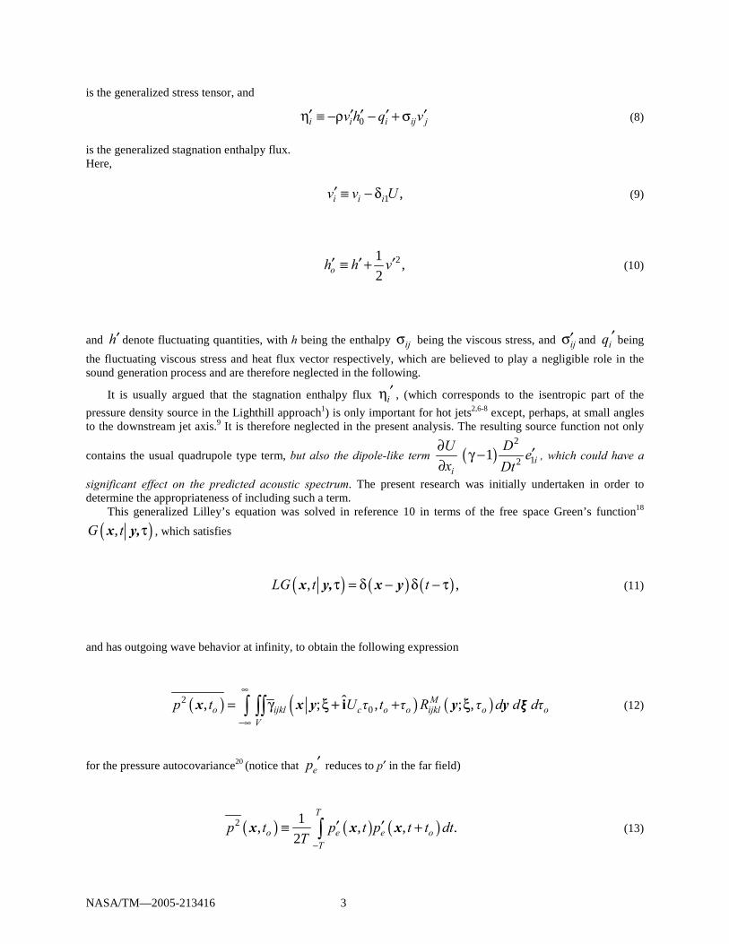
is the generalized stress tensor, and

0i i i ij jv h q v′ ′ ′ ′ ′η ≡ −ρ − + σ (8)

is the generalized stagnation enthalpy flux. Here, 1 ,i i iv v U′ ≡ − δ (9)

21 ,2oh h v′ ′ ′≡ + (10)

and h′ denote fluctuating quantities, with h being the enthalpy ijσ being the viscous stress, and ij′σ and iq ′ being the fluctuating viscous stress and heat flux vector respectively, which are believed to play a negligible role in the sound generation process and are therefore neglected in the following.

It is usually argued that the stagnation enthalpy flux i′η , (which corresponds to the isentropic part of the

pressure density source in the Lighthill approach1) is only important for hot jets2,6-8 except, perhaps, at small angles to the downstream jet axis.9 It is therefore neglected in the present analysis. The resulting source function not only

contains the usual quadrupole type term, but also the dipole-like term i

Ux

∂∂

( )2

121 iD eDt

′γ − , which could have a

significant effect on the predicted acoustic spectrum. The present research was initially undertaken in order to determine the appropriateness of including such a term. This generalized Lilley’s equation was solved in reference 10 in terms of the free space Green’s function18

( ),G t τx y, , which satisfies

( ) ( ) ( ), ,LG t tτ = δ − δ − τx y, x y (11)

and has outgoing wave behavior at infinity, to obtain the following expression

( ) ( ) ( )20

ˆ, ; , ; ,Mo ijkl c o o ijkl o o

V

p t U τ t τ R τ d d dτ∞

−∞

= γ +∫ ∫∫x x y y y ξξ + ξi (12)

for the pressure autocovariance20 (notice that ep ′ reduces to p′ in the far field)

( ) ( ) ( )2 1, , , .2

T

o e e oT

p t p t p t t dtT −

′ ′≡ +∫x x x (13)

NASA/TM—2005-213416 4

The symbol V denotes integration over all space; T denotes some large but finite time interval,

ˆc oU τ≡ −ξ η i (14)

denotes a moving frame coordinate system,

( ) ( ) ( )0 0 1 1 1, , , , ,ijkl ij o o klt t t t dt∞

−∞

γ + τ ≡ γ + + τ γ +∫x y;η x y x y η (15)

and the propagation factor ( ),kl tγ x y is defined in reference 10. ( ); ,Mijkl 0R τy ξ is a moving frame correlation

tensor, which is defined in terms of the fixed frame density-weighted, fourth-order, two-point, and time-delayed fluctuating velocity correlation

( ) ( ) ( )1; , , ,2

T

ijkl o i j k l oT

R τ v v τ v v τ τ dτT −

′ ′ ′ ′≡ ρ ρ + +∫y y yη η (16)

and the second order fixed frame density weighted correlation

( ) ( ) ( )1; , ,2

T

ij o i j oT

R v v dT −

′ ′τ ≡ ρ τ ρ + τ + τ τ∫y y, yη η (17)

by

( ) ( ) ( ) ( )ˆ ˆ; , ; , ; ,0 ; ,0 .Mijkl 0 ijkl c o o ij kl c oR τ R U τ τ R R U τ≡ −y y y y +i 0 i 0ξ ξ + ξ + (18)

The indicated arguments refer to all three terms preceding the parentheses. Our interest is in the far field spectrum

( ) ( )21 , ,2

oi to oI e p t dt

∞ω

ω−∞

≡π ∫x x (19)

which can be calculated by taking the Fourier transform of equation (12) and using the convolution theorem21 to obtain

NASA/TM—2005-213416 5

( ) ( ) ( ) ( )* ˆ2 ; ; , , ,oi τ Mij kl c o ijkl o o

V

I U τ e R τ d dτ∞

− ωω

−∞

= π Γ ω Γ + + ω∫ ∫x y x y x y i yξ ξ ξ (20)

where

( ) ( ) ( )1 ,2

i tij ije t d tω −τ

−∞

Γ ≡ γ − τ − τπ ∫ x y (21)

is the Fourier transform of ijγ (we use capital letters to denote Fourier transform of the corresponding lower case

quantity) and we introduced ( )Iω |x y , the acoustic spectrum at x due to a unit volume of turbulence at y, i.e.,

( ) ( )V

I I dω ω= ∫x x y y, (22)

in order to simplify the formulas. The relevant far field expansion of ijΓ is given in reference 10. The only approximation made up to this point is the neglect of the enthalpy and viscous source terms, but equation (20) will depend on the turbulent source correlations only through

( ) ( ), , ,Mijkl o ijkl o

V

R dτ ≡ τ∫y y ξξR (23)

if variations in retarded time across the correlation volume are neglected, i.e., if ( )ˆ ;kl cU∗Γ + + τ ωx y iV is

assumed to be constant over the correlation volume.3 However, the definitions (14) and (18) imply that the integration variable in equation (23) can be changed back to η , which means that

( ) ( ) ( ) ( ), , , ; ,0 ; ,0ijkl o ijkl o ij klV

R R R d⎡ ⎤τ ≡ τ −⎣ ⎦∫y y y y + η0 0R O O (24)

Equation (20) can now be rearranged into the simpler form

( ) ( ) ( ) ( )( )22 2 sin * , 1 cos ,as ,ij kl ijkl cI M x

x c∗

ω ⊥ ⊥∞

π πω⎛ ⎞→ θ Γ Γ Φ − θ ω → ∞⎜ ⎟⎝ ⎠

x y x y x y y (25)

NASA/TM—2005-213416 6

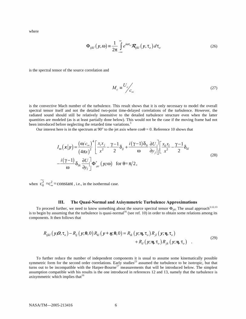
where

( ) ( )1, ,2

oiijkl ijkl o oe d

∞ωτ

−∞

Φ ω ≡ τ τπ ∫y yR (26)

is the spectral tensor of the source correlation and

cc

UM c∞≡ (27)

is the convective Mach number of the turbulence. This result shows that it is only necessary to model the overall spectral tensor itself and not the detailed two-point time-delayed correlations of the turbulence. However, the radiated sound should still be relatively insensitive to the detailed turbulence structure even when the latter quantities are modeled (as is at least partially done below). This would not be the case if the moving frame had not been introduced before neglecting the retarded time variations.3

Our interest here is in the spectrum at 90° to the jet axis where cosθ = 0. Reference 10 shows that

( ) ( )( )

( )

( ) ( )

41

2 2 2

1

11 12 24

1for = 2,

ijkl

i j i k lij kl

j

kl

x xc i x xUIyx xx

i Uy

∞ω

∗

⎤ω γ − δ⎡ γ − ∂ γ −⎡= − δ + − δ⎥⎢ ⎢ω ∂ ⎣π ⎥⎣ ⎦γ − ⎤∂− δ Φ ω θ π⎥ω ∂ ⎦

x y

y;

(28)

when 2 20 c =c = c o nstant∞ , i.e., in the isothermal case.

III. The Quasi-Normal and Axisymmetric Turbulence Approximations To proceed further, we need to know something about the source spectral tensor Φijkl. The usual approach3,12,13

is to begin by assuming that the turbulence is quasi-normal16 (see ref. 10) in order to obtain some relations among its components. It then follows that

( ) ( ) ( ) ( ) ( )

( ) ( ), , ; ,0 ; ,0 ; , ; ,

; , ; , .ijkl o ij kl ik o jl o

il o jk o

R R R R R

R R

τ − = τ τ

+ τ τ

y y y + η y y

y y

0 0 η η

η η

O (29)

To further reduce the number of independent components it is usual to assume some kinematically possible symmetric form for the second order correlations. Early studies23 assumed the turbulence to be isotropic, but that turns out to be incompatible with the Harper-Bourne17 measurements that will be introduced below. The simplest assumption compatible with his results is the one introduced in references 12 and 13, namely that the turbulence is axisymmetric which implies that16

NASA/TM—2005-213416 7

( ) ( )0 0 0 1 1 0 1 1; ,ij o i j ij i j j j j iR A B C Dτ = η η + δ + δ δ + δ η + δ ηy η (30)

where the symbols A0, B0, C0, and D0 denote functions of y, 0τ , and 2 22 3⊥η ≡ η + η ; A0, B0 and C0 denote even

functions of the latter quantity whileD0 denotes an odd function. This model is chosen because it is the most general of those whose mathematical properties have been studied in the literature and because it reflects the fact that the cross flow velocity components tend to be much more similar to one another than to the stream-wise component (even for non-axysymmetric flows). Inserting equation (30) into equation (29) and inserting the result into equation (25) via equations (24) and (26) yields (after a straightforward but tedious calculation that follows along the lines of the one in appendix A of ref. 12)

( )( )

( ) ( )

2

4 22

1 2 3 4

4

12 1 1 ,2

I x

Mc c

ω

∞ ∞

⎜ π

⎡ ⎤⎛ ⎞ ⎡ ⎤ω γ − ω⎛ ⎞= Φ − γ − Φ + Φ + γ − ∇ Φ⎢ ⎥⎜ ⎟ ⎢ ⎥⎜ ⎟⎝ ⎠⎝ ⎠ ⎢ ⎥ ⎣ ⎦⎣ ⎦

x y

(31)

where

( )21 22

1 , , ,2

oio o

V

e R d d∞

− ωτ

−∞

Φ ≡ τ τπ ∫ ∫ y η η (32a)

( )2 2 22 23 12 22

1 ,2

oio

V

e R R R d d∞

− ωτ

−∞

Φ ≡ + + τπ ∫ ∫ η (32b)

( )2 2 2 23 12 23 11 22

1 4 2 2 ,2

oio

V

e R R R R d d∞

− ωτ

−∞

Φ ≡ + + + τπ ∫ ∫ η (32c)

and

( )24 12 11 22

12

oio

V

e R R R d d∞

− ωτ

−∞

Φ ≡ + τπ ∫ ∫ η (32d)

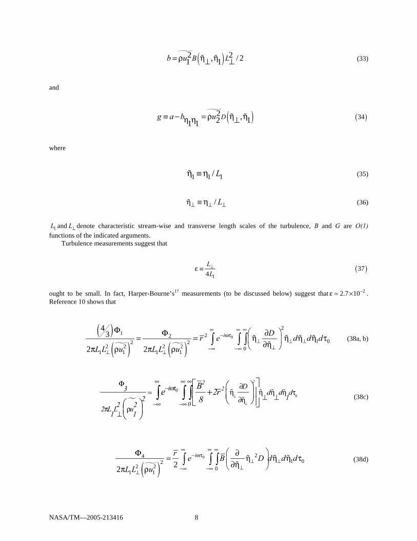
are seemingly independent spectral functions. However, the coefficients A, B, C, and D are not all independent and, when compressibility effects are neglected (i.e., when ρ is treated as a constant), these turbulence correlations can be expressed in terms of two independent scalar functions of y, 0τ , ⊥η , and 1η , say a and b,14,15,24 which scale like

NASA/TM—2005-213416 8

( )2 2, / 21 1B Lb u= ρ η η⊥ ⊥ (33)

and

( )2 ,2 11 1Dg a b u≡ − = ρ η ηη η ⊥ ( )34

where

1 1 1/ Lη ≡ η (35)

/ L⊥ ⊥ ⊥η ≡ η (36)

1L and L⊥ denote characteristic stream-wise and transverse length scales of the turbulence, B and G are O(1)

functions of the indicated arguments. Turbulence measurements suggest that

14

LL⊥ε ≡ ( )37

ought to be small. In fact, Harper-Bourne’s17 measurements (to be discussed below) suggest that 22.7 10−ε × . Reference 10 shows that

( )

( ) ( )0

21 22

1 02 22 2 2 2 0

1 1 1 1

43

2 2

i Dr e d d dL L u L L u

∞ ∞ ∞− ωτ

⊥ ⊥ ⊥⊥−∞ −∞

⊥ ⊥

Φ ⎛ ⎞Φ ∂= = η η η η τ⎜ ⎟∂η⎝ ⎠π ρ π ρ∫ ∫ ∫ (38a, b)

2

00

22i

0

D3 d d d12

2 22 L L u1 1

B2r

8e ⊥

⊥

∞ ∞ ∞− ωτ

−∞ −∞

Φ ∂= η η η η τ

⊥ ⊥∂ηπ ρ

⊥

+⎤⎡ ⎛ ⎞⎥⎢ ⎜ ⎟

⎝ ⎠ ⎥⎣ ⎦⎛ ⎞⎜ ⎟⎝ ⎠

∫ ∫ ∫ (38c)

( )0 24

1 022 2 0

1 122

ir e B D d d dL L u

∞ ∞ ∞− ωτ

⊥ ⊥⊥−∞ −∞

⊥

⎛ ⎞Φ ∂= η η η τ⎜ ⎟∂η⎝ ⎠π ρ∫ ∫ ∫ (38d)

NASA/TM—2005-213416 9

when ( )2O ε terms are neglected. The ratio r is defined by

2 22 1 .r u u≡ ρ ρ (39)

Lacking any specific data to the contrary, it seems reasonable to suppose that

( ) ( )2 2 2 222 0 11

1 1, , ( ) ( ) , ,o oi io o o o

V V

e R d d r r e R d d∞ ∞

− ωτ − ωτ

−∞ −∞

τ τ Γ Φ ≡ Γ τ τπ π∫ ∫ ∫ ∫y yη η = η η (40)

where Γ is a constant. Equation (31) then becomes

( )( ) ( ) ( )2

22 2 202 ,oI xc C U

cω ∞∞

⎛ ⎞ω ⎡ ⎤⏐ π = Φ ω ω + κ ∇⎜ ⎟ ⎢ ⎥⎣ ⎦⎝ ⎠yx y (41)

where

( )2 2

2 20

2 3 1 1 12 ( ) 1 23 4 2 2 2

C r⎤γ − γ −⎡ ⎛ ⎞ ⎛ ⎞≡ Γ − γ − + +⎥⎜ ⎟ ⎜ ⎟⎢⎣ ⎝ ⎠ ⎝ ⎠⎥⎦

(42)

is a constant, i.e., independent of ω ,and

0

0

21 0

0

0 21 0

0

21 1

2

i

i

r e B D d d d

Ce B d d d

∞ ∞ ∞− ωτ

⊥ ⊥⊥−∞ −∞

∞ ∞ ∞− ωτ

⊥ ⊥−∞ −∞

κ ≡

⎛ ⎞∂ η η η τ⎜ ⎟∂ηγ −⎛ ⎞ ⎝ ⎠⎜ ⎟⎝ ⎠

η η η τ

∫ ∫ ∫

∫ ∫ ∫

(43)

IV. The Harper-Bourne Spectrum The results cannot be made more explicit without inputting more specific information about the turbulence structure. This is accomplished with the aid of some recent measurements17 of the two-point fourth-order stream-wise velocity correlation spectra along the centerline of the mixing layer in a low Mach number jet, which would most closely correspond to

( ) ( )211

1, , , ,oio o oH e R d

∞− ωτ

−∞

ω ≡ τ τπ ∫y yη η (44)

NASA/TM—2005-213416 10

with the quasi-normal approximation that is being used in the present analysis. Harper-Bourne17 divided 0H into the three components (see his eqs. (2.5) and (2.7) on p. 2)

( ) 1

1, , , , , pi

o oH H R el l

ωτ⊥

⊥

⎛ ⎞η η= ω ω⎜ ⎟⎝ ⎠

y y0 (45)

where 1l , l⊥ are the spectral stream-wise and transverse length scales (not necessarily the same as the time domain length scales 1L and L⊥ introduced above) and

1 .pcU

ητ (46)

No assumption is made about the decomposition of the correlations into products of their space and time components with this approach. The first factor can be evaluated from his measurements of ( )1111 0, ,R τy 0 , which are reasonably well

represented by the exponential oe−λ τ . But reference 19 shows that ( )1111 0, ,R τy 0 does not in reality have a sharp

cusp at 0 0τ = . A better representation would therefore be

( )0 00 0

1111 0

erfc. + erfc.2 2, , ,2erfc.

e eR

−λτ λτλτ λτ⎛ ⎞ ⎛ ⎞β − β +⎜ ⎟ ⎜ ⎟β β⎝ ⎠ ⎝ ⎠τ =β

y 0 (47)

which behaves like oe−λ τ for large 0τ and reduces to this quantity when 0β = , but smoothes out the cusp at

0 0τ = . It therefore follows that20

( )( )2/4

12 2 2, , .

(exp. erfc. )( )ou eH

− βω λλρω =π β β λ + ω

y 0 (48)

Inserting these into equation (46) and using the result in equations (41) and (42) shows that

( )( ) ( ) ( )2 2/4 2 3 2

1 1 120 2 4 2 2 2

2 ,,

(exp. erfc. )( )

cu e U U l l R lI C

x c

− βω λ⊥

ω∞

⎡ ⎤λρ ω + κ ∇⎢ ⎥⎣ ⎦⏐ =β β λ + ω ω

yx y (49)

where

NASA/TM—2005-213416 11

( ) ( ) 2 11, 2 , , ,1 1 10

i lR l R e d d

∞ ∞ − π η≡ π η η η η η∫ ∫ ⊥ ⊥ ⊥

−∞y y ( )50

and 1l and l⊥ are defined by

11

c

ll

2 Uω

≡π

(51)

and

.2 c

llU⊥

⊥ω≡π

(52)

Harper-Bourne obtains the best fit to his data with the non-separable form

2 41 ,R e ⊥− η +η= (53)

which can be inserted into equation (50) to obtain

( )3

2 21

.

2 1 2

R

l

π=⎡ ⎤+ π⎢ ⎥⎣ ⎦

(54)

Harper-Bourne’s figure 13 shows that while 1l and l⊥ are constant at relatively low frequencies, it is the scaled

length scales il and l⊥ that become constant as ω → ∞ . The data is well represented by the functions ( )21 1 1

2 2St

J

l eU

−ω ≈ −π

(55)

and

( )0.50.15 1 ,2

St

J

l eU

−⊥ω ≈ −π

(56)

where

NASA/TM—2005-213416 12

2J

JDSt U

ω≡ π (57)

and JD denotes the jet diameter.

V. Extension of the Harper-Bourne Data Unfortunately, all of Harper-Bourne’s data are taken at a single point in a very low Mach number jet, while practical interest is in much higher Mach number flows and the acoustic predictions require information about the turbulence over the entire noise producing region of the jet. We therefore attempt to extend his data by using some modeling assumptions along with the Wind code developed by NASA Glenn Research Center and the U.S.A.F. Arnold Engineering Development Center, which is a RANS code with a standard k − ε turbulence model. To this end, we first assume that the time scale 1−λ that appears in equation (49) is proportional to the k − ε time scale k

ε ,

i.e., we put 1 kC− τλ ≈ ε (58)

where Cτ is an adjustable constant.

Equations (55) and (56) are extended by assuming that the time and velocity scales JJ

DU and JU are

proportional to the k − ε time and length scales kε and

12k respectively to obtain

⎥⎦

⎤⎢⎣

⎡⎟⎠⎞

⎜⎝⎛−−≈

πεω

πω

2exp1

22/11 kCkCl Sl (59)

and

1 20 3 1 0 252 2

l / Sl k. C k exp . C ,⊥ ⎡ ⎤ω ω⎛ ⎞≈ − −⎢ ⎥⎜ ⎟π πε⎝ ⎠⎣ ⎦ (60)

where lC and SC are constants. Figure 1 shows the RANS (WIND code) solution for a 2 in. diameter cold jet at the jet exit Mach number of 0.18 for which Harper-Bourne carried out his measurements. The two constants lC and

SC are determined by requiring that equations (55) and (59) be in reasonable agreement with the data at the measurement point ( 1 4 0Jx / D . ,= 2 0 50Jx / D .= ). A reasonably good approximation is obtained by selecting

lC ≈ 3.0 and 0.50SC ≈ . We neglected the difference in exponents between (59) and (60) but plan to remedy this oversight in the near future.

The velocity ratio r is typically close to ½ in. most cases and we shall use this value in our computations. The constant oC is related to the ratio rΓ (defined implicitly by eq. (40)) by eq. (43), which for 1.4γ = becomes

( )22 0.43 0.013oC r≈ Γ + (61)

NASA/TM—2005-213416 13

Unfortunately, Harper- Bourne only measured the stream-wise and not the transverse velocity correlations so that Γ

is essentially unknown. But if we assume, as in reference 10, that ( ) 2 21/ 2 , oB D a e ⊥−η= = η τ then this quantity

is equal to 3 and it follows that

2 0.1472.oC ≈ (62)

We treat , , and oC Cτ β as adjustable constants, whose determination is described in the next section. It is necessary to specify the square root in equation (43) in order to fix κ . Again, Harper- Bourne does not provide enough data to ascertain this quantity, but it becomes equal to ½ in. and equation (43), therefore, becomes

0.1oCκ ≈ (63)

when, as before, it is assumed that 1.4γ = and ( ) 2 21/ 2 , oB D a e ⊥−η= = η τ .

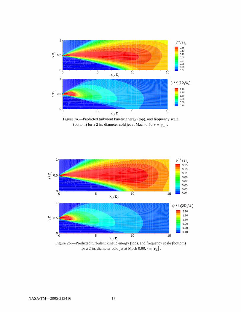
VI. Comparison with Measurements The far-field spectra at 90° to the jet axis were calculated from equations (49) and (54) at 1 Jy = 100D for Mach 0.50, 0.90, and 1.5 cold jets. As in the JeNo code,15,21 the local result (49) was summed over all source points within the noise producing region of the jet in order to predict the actual sound field. RANS solutions for the relevant nozzles were obtained from the WIND code with upstream boundary conditions specified in terms of the stagnation pressure and temperature at the nozzle plenum entrance. The predicted turbulent kinetic energy distribution and the corresponding time-scale for the three jets are shown in figure 2.

The calculated 90° acoustic spectra are compared with the subsonic SHJAR data recently acquired at NASA Glenn Research Center and correctly expanded supersonic data obtained at Langley Research Center in figures 3 through 5. Atmospheric attenuation was removed from all measurements in order to make a lossless comparison

with predictions. We expect the parameters lC and SC , which were determined from the Mach 0.18 jet RANS solution, to be independent of both Reynolds number and Mach number. The adjustable constants , , and oC Cτ β

were determined by obtaining the best fit with the Mach 0.5 data. The resulting values of Cτ and β turn out to be

0.35 and 0.10 respectively. The scale factor oC turns out to be 2 0.133oC ≈ , which is in remarkably good agreement with the value calculated from equation (61). The calculated spectra are in excellent agreement with the subsonic data over the entire frequency range. The agreement is not quite as good for the supersonic case, but it is likely that this data contains a small amount of shock associated noise that is not accounted for by the theory. Equation (63) implies that 0 27.κ ≈ when 2 0.133oC ≈ . Figure 4 (with 0 9.κ ≈ ) shows that there is very little difference between the results obtained with κ given by this equation and those obtained with κ = 0. Equation (49) shows that 4~ ωωI as 0→ω in the latter case, which is consistent with the conventional wisdom that, at least for cold jets, the sideline noise is dominated by a quadrupole- type source as originally proposed by Lighthill.

VII. Discussion A simpler and, we believe, more elegant form of Lilley’s equation was derived in reference 19 by introducing the new dependent variable

NASA/TM—2005-213416 14

( ) 11p

pγπ ≡ − (64)

to obtain

1

2 ,ji

i j

ffD ULDt x x x

∂∂ ∂π = −∂ ∂ ∂

(65)

where

( ) ( )1 1 .i i jj i

f v v hx x∂ ∂π′ ′ ′≡ − + π − γ −

∂ ∂ (66)

L is defined by equation (3) and iv′ is defined by equation (9). In this context it is usual to neglect the dipole-like

term ( )1i

hx

∂π′γ −∂

rather than the dipole-like term ( )2

21 j

j

DxDt

′∂ηγ −

∂ for cold air jets. It was also shown in

reference 19 that this dipole-like term will not even appear in equation (66) if 2c is replaced by ( )2 2c c ′+ (where

( ) ( )2 1c h′ ′= γ − denotes the fluctuation in the squared sound speed) in the operator L defined by equation (3), so its

neglect can also be interpreted to mean that the sound speed fluctuations have a negligible effect (relative to the mean) on the acoustic propagation. Since equations (2) and (65) are both exact, any differences in the predictions must be attributable to the neglect of these terms. When the preceding analysis is applied to the present equations (i.e., equations (64) to (66) rather than equation (2)), the final result is still given by equation (41) but with 0κ = , a slightly different definition of the density weighted source correlations, and

( )22 1 ,4oC r= Γ (67)

which becomes

2 0.187,oC ≈ (68)

when the values Γ and r obtained in the previous section are inserted-a result that is fairly close to the previous value. The principal difference between these predictions is therefore due to the second term in the factor

( )22 U⎡ ⎤ω + κ ∇⎢ ⎥⎣ ⎦, which does not significantly affect the high frequency behavior of the solution but has the

potential of causing Iω to exhibit the dipole-like behavior

2 0I asω ω ω →∼ (69a)

in the formulation discussed in this paper rather than the quadrupole-like behavior

NASA/TM—2005-213416 15

4 0I asω ω ω →∼ (69b)

that always occurs when the predictions are based on equations (65) and (66). But the computations and data comparisons of the previous section show that the second term in this factor is relatively small for cold jets and that good agreement is achieved independently of whether that term is included. This is because the low frequency roll off of the acoustic spectrum is primarily determined by the peak frequency distribution of the local spectra and not by their low frequency asymptotes. We note, however, that the value of oC given by equation (62) is slightly closer to the “fitted” value than the one given by equation (68), but-given the uncertainty of the approximations used in the source modeling-this difference is not large enough to distinguish between these two forms of the acoustic analogy.

VII. Concluding Remarks The research was initially motivated by the need to distinguish between the two forms of the acoustic analogy described above. Unfortunately the results turned out to be inconclusive-with both forms of the analogy yielding excellent agreement with the data. Our hope is that similar comparisons for hot jets or jets with more complex flow fields will provide the required selectivity. But until this is done, our recommendation would be to base the jet noise predictions on the formulation (65) and (66), as was done in reference 21, since this leads to much simpler formulas-especially at angles other than 90°.

Finally, it is worth noting that the adjustable constant β, which measures the curvature of the temporal autocovariance at 0τ = , is relatively small and is therefore consistent with experimentally observed turbulence spectra.20 It is, however, somewhat puzzling that the high frequency roll off of the predicted acoustic spectra turns out to be fairly sensitive to this parameter. It is also rather unfortunate, because this quantity is difficult to measure with any accuracy.

References 1Lighthill, M.J., “On Sound Generated Aerodynamically: I. General Theory,” Proceedings R. Society Lond., A 211, 1952, pp. 564–587. 2Lilley, G.M., “On the Noise from Jets,” Noise Mechanism, AGARD–CP–131, 1974, pp. 13.1–13.12. 3Ffowcs William, J.E., “The Noise from Turbulence Convected at High Speed,” Phil. Trans. Roy. Soc., A 225, 1963, pp. 469–503. 4Harper-Bourne, M., “Jet Noise Turbulence Measurements,” AIAA Paper 2003–3214, 2003. 5Goldstein, M.E., “A Generalized Acoustic Analogy,” Journal of Fluid Mechanics, vol. 488, 2003, pp. 315–333. 6Lilley, G.M., “The Radiated Noise from Isotropic Turbulence with Applications to the Theory of Jet Noise,” Journal of Sound Vibration, vol. 190, 1996, pp. 463–476. 7Morfey, C.L., Szewczyk, V.M., and Fisher, B.J., “New Scaling Laws for Hot and Cold Jet Mixing Noise Based on a Geometric Acoustics Model,” Journal of Sound and Vibration, vol. 46, no. 1, 1976, pp. 79–103. 8Lilley, G.M., “Jet Noise: Classical Theory and Experiments” in Aeroacoustics of Flight Vehicles, H. Hubbard ed., vol. 1 NASA RP-1258, and WRDC TR-90-3052, 1991, pp. 211–289. 9Freund, J.B., “Turbulent Jet Noise: Shear Noise, Self-Noise, and Other Contributions,” AIAA Paper 2002–2423, 2002. 10Goldstein, M.E., “The 90° Acoustic Spectrum of a High Speed Air Jet”, AIAA Journal, vol. 42, no. 11, Nov. 2004. 11Goldstein, M.E. and Rosenbaum, B.M., “Emission of Sound from Turbulence Converted by a Parallel Flow in the Presence of Solid Boundaries,” NASA TN D–7118, 1973. 12Goldstein, M.E. and Rosenbaum, B., “Effect of Anisotropic Turbulence on Aerodynamic Noise,” Journal of the Acoustical Society of America, vol. 54, no. 3, 1973, pp. 630–645.

NASA/TM—2005-213416 16

13Kerschen, E.J., “Constraints on the Invariant Function of Axisymmetric Turbulence,” AIAA Journal, vol. 21, no. 7, 1983, pp. 978–985. 14Lindborg, E., “Kinematics of Homogeneous Axisymmetric Turbulence,” Journal of Fluid Mechanics, vol. 302, 1995, pp. 179–201. 15Khavaran, A., “Role of Anisotropy in Turbulent Mixing Noise,” AIAA Journal, vol. 37, no. 7, 1999, pp. 832–841. 16Batchelor, G.K., “Theory of Homogeneous Turbulence,” Cambridge University Press, 1953. 17Pridmore-Brown, “Sound Propagation in a Fluid Flowing Through an Attenuating Duct,” Journal of Fluid Mechanics, vol. 4, 1958, pp. 393–406. 18Morse, P.M. and Feshbach, H., “Methods of Theoretical Physics,” McGraw-Hill, 1953. 19Goldstein, M.E., “An exact form of Lilley’s equation with a velocity quadrupole/temperature dipole source term” Journal of Fluid Mechanics, vol. 443, 2001, pp. 231–236. 20Pope, S.B., “Turbulent Flows,” Cambridge University Press, 2000, pp. 70 and 144. 21Khavaran, A., Bridges, J., and Freund, J.B., “A Parametric Study of Fine-Scale Turbulence Mixing Noise,” NASA/TM—2002-211696, 2002. 22Norum, T. NASA-Langley Jet Noise Lab Generic Nozzle Narrow Band Spectra, vol. 1, 1994 (unpublished, available electronically).

x1 / DJ

r/D

J

0 5 10 150

0.5

1

2.101.701.300.900.500.10

(ε/k)(2DJ/UJ)

x1 / DJ

r/D

J

0 5 10 150

0.5

10.150.130.110.090.070.050.030.01

k 0.5 / UJ

Figure 1.—Predicted turbulent kinetic energy (top), and frequency scale

(bottom) in a Mach 0.18 cold jet. r .⊥≡ y

NASA/TM—2005-213416 17

x1 / DJ

r/D

J

0 5 10 150

0.5

1

0.150.130.110.090.070.050.030.01

k0.5/ UJ

x1 / DJ

r/D

J

0 5 10 150

0.5

1

2.101.701.300.900.500.10

(ε / k)(2DJ/UJ)

Figure 2a.—Predicted turbulent kinetic energy (top), and frequency scale

(bottom) for a 2 in. diameter cold jet at Mach 0.50. r ⊥≡ y .

x1 / DJ

r/D

J

0 5 10 150

0.5

1

2.101.701.300.900.500.10

(ε / k)(2DJ/UJ)

x1 / DJ

r/D

J

0 5 10 150

0.5

1

0.150.130.110.090.070.050.030.01

k0.5 / UJ

Figure 2b.—Predicted turbulent kinetic energy (top), and frequency scale (bottom)

for a 2 in. diameter cold jet at Mach 0.90. r ⊥≡ y .

NASA/TM—2005-213416 18

x1 / DJ

r/D

J

0 5 10 150

0.5

1

0.160.140.120.100.070.050.030.01

k0.5 / UJ

x1 / DJ

r/D

J

0 5 10 150

0.5

1

2.101.701.300.900.500.10

(ε /k)(2DJ/UJ)

Figure 2c.—Predicted turbulent kinetic energy (top), and frequency scale (bottom)

for a Mach 1.50 convergent-divergent nozzle with 1.68 in. exit diameter. r ⊥≡ y .

Figure 3.—Spectrum at 90° and at R/DJ = 100 for a Mach 0.50 cold jet. Prediction (dashed line); data (solid line), 2f ω≡ π , R ≡ y .

f DJ / UJ

10Lo

g(U

JD

J_1P

2/p

r2),

dB

10-1 100 101404550556065707580

NASA/TM—2005-213416 19

Figure 4.—Spectrum at 90° and at R/DJ = 100 for a Mach 0.90 cold jet. Prediction with 0.0=κ (dashed line); 90.0=κ (dash-dot);

data (solid line), 2f ω≡ π , R ≡ y .

Figure 5.—Spectrum at 90° and at R/DJ = 100 for Mach 1.5 cold jet. Prediction (dash-dot); data (solid line), 2f ω≡ π , R ≡ y .

f DJ / UJ

10Lo

g(U

JD

J_1P

2/p

r2),

dB

10-2 10-1 100 10180

85

90

95

100

105

110

115

f DJ / UJ

10Lo

g(U

JD

J_1P

2/p

r2),

dB

10-2 10-1 100 10160

65

70

75

80

85

90

95

This publication is available from the NASA Center for AeroSpace Information, 301–621–0390.

REPORT DOCUMENTATION PAGE

2. REPORT DATE

19. SECURITY CLASSIFICATION OF ABSTRACT

18. SECURITY CLASSIFICATION OF THIS PAGE

Public reporting burden for this collection of information is estimated to average 1 hour per response, including the time for reviewing instructions, searching existing data sources,gathering and maintaining the data needed, and completing and reviewing the collection of information. Send comments regarding this burden estimate or any other aspect of thiscollection of information, including suggestions for reducing this burden, to Washington Headquarters Services, Directorate for Information Operations and Reports, 1215 JeffersonDavis Highway, Suite 1204, Arlington, VA 22202-4302, and to the Office of Management and Budget, Paperwork Reduction Project (0704-0188), Washington, DC 20503.

NSN 7540-01-280-5500 Standard Form 298 (Rev. 2-89)Prescribed by ANSI Std. Z39-18298-102

Form ApprovedOMB No. 0704-0188

12b. DISTRIBUTION CODE

8. PERFORMING ORGANIZATION REPORT NUMBER

5. FUNDING NUMBERS

3. REPORT TYPE AND DATES COVERED

4. TITLE AND SUBTITLE

6. AUTHOR(S)

7. PERFORMING ORGANIZATION NAME(S) AND ADDRESS(ES)

11. SUPPLEMENTARY NOTES

12a. DISTRIBUTION/AVAILABILITY STATEMENT

13. ABSTRACT (Maximum 200 words)

14. SUBJECT TERMS

17. SECURITY CLASSIFICATION OF REPORT

16. PRICE CODE

15. NUMBER OF PAGES

20. LIMITATION OF ABSTRACT

Unclassified Unclassified

Technical Memorandum

Unclassified

National Aeronautics and Space AdministrationJohn H. Glenn Research Center at Lewis FieldCleveland, Ohio 44135–3191

1. AGENCY USE ONLY (Leave blank)

10. SPONSORING/MONITORING AGENCY REPORT NUMBER

9. SPONSORING/MONITORING AGENCY NAME(S) AND ADDRESS(ES)

National Aeronautics and Space AdministrationWashington, DC 20546–0001

Available electronically at http://gltrs.grc.nasa.gov

January 2005

NASA TM—2005-213416AIAA–2005–0415

E–14937

Cost Center 2250000004

25

Acoustic Source Modeling for High Speed Air Jets

Marvin E. Goldstein and Abbas Khavaran

Jet noise; Turbulence; Acoustics

Unclassified -UnlimitedSubject Categories: 01, 34, and 71 Distribution: Nonstandard

Prepared for the 43rd Aerospace Sciences Meeting and Exhibit sponsored by the American Institute of Aeronautics andAstronautics, Reno, Nevada, January 10–13, 2005. Marvin E. Goldstein, NASA Glenn Research Center; and AbbasKhavaran, QSS Group, Inc., 21000 Brookpark Road, Cleveland, Ohio 44135. Responsible person, Marvin E. Goldstein,organization code R, 216–433–5825.

The far field acoustic spectra at 90° to the downstream axis of some typical high speed jets are calculated from twodifferent forms of Lilley’s equation combined with some recent measurements of the relevant turbulent source function.These measurements, which were limited to a single point in a low Mach number flow, were extended to other conditionswith the aid of a highly developed RANS calculation. The results are compared with experimental data over a range ofMach numbers. Both forms of the analogy lead to predictions that are in excellent agreement with the experimental data atsubsonic Mach numbers. The agreement is also fairly good at supersonic speeds, but the data appears to be slightlycontaminated by shock-associated noise in this case.