Acoustic Scattering from a Sphere

Steve Turley

November 24, 2006

Contents

1 Introduction 2

1.1 Boundary Conditions . . . . . . . . . . . . . . . . . . . . . . . . . . . . . . . . . . . . . . . . . 21.2 Green's Function . . . . . . . . . . . . . . . . . . . . . . . . . . . . . . . . . . . . . . . . . . . 31.3 Far Field . . . . . . . . . . . . . . . . . . . . . . . . . . . . . . . . . . . . . . . . . . . . . . . 31.4 Solutions in Spherical Coordinates . . . . . . . . . . . . . . . . . . . . . . . . . . . . . . . . . 4

2 Potentials 4

3 Scattering Theory 6

3.1 Integral Equations . . . . . . . . . . . . . . . . . . . . . . . . . . . . . . . . . . . . . . . . . . 63.2 Applying Boundary Conditions . . . . . . . . . . . . . . . . . . . . . . . . . . . . . . . . . . . 7

3.2.1 Dirichlet Problem . . . . . . . . . . . . . . . . . . . . . . . . . . . . . . . . . . . . . . 73.2.2 Neuman Problem . . . . . . . . . . . . . . . . . . . . . . . . . . . . . . . . . . . . . . . 93.2.3 Penetrable Scatterer . . . . . . . . . . . . . . . . . . . . . . . . . . . . . . . . . . . . . 10

4 Balloon Scattering 11

5 Results 11

5.1 Soft Sphere . . . . . . . . . . . . . . . . . . . . . . . . . . . . . . . . . . . . . . . . . . . . . . 115.1.1 Far Field . . . . . . . . . . . . . . . . . . . . . . . . . . . . . . . . . . . . . . . . . . . 125.1.2 Near Field . . . . . . . . . . . . . . . . . . . . . . . . . . . . . . . . . . . . . . . . . . . 17

5.2 Hard Sphere . . . . . . . . . . . . . . . . . . . . . . . . . . . . . . . . . . . . . . . . . . . . . . 185.2.1 Far Field . . . . . . . . . . . . . . . . . . . . . . . . . . . . . . . . . . . . . . . . . . . 205.2.2 Near Field . . . . . . . . . . . . . . . . . . . . . . . . . . . . . . . . . . . . . . . . . . . 20

5.3 Penetrable Scatters . . . . . . . . . . . . . . . . . . . . . . . . . . . . . . . . . . . . . . . . . . 205.3.1 Far Field . . . . . . . . . . . . . . . . . . . . . . . . . . . . . . . . . . . . . . . . . . . 205.3.2 Near Field . . . . . . . . . . . . . . . . . . . . . . . . . . . . . . . . . . . . . . . . . . . 26

5.4 Balloon . . . . . . . . . . . . . . . . . . . . . . . . . . . . . . . . . . . . . . . . . . . . . . . . 26

References 26

List of Figures

1 Dierential cross section for scattering from an acoustically soft sphere of radius 0.1 wavelengths. 132 Dierential cross section for scattering from an acoustically soft sphere of radius 1.0 wavelength. 143 Dierential cross section for scattering from an acoustically soft sphere of radius 3.0 wavelengths. 154 Dierential cross section for scattering from an acoustically soft sphere of radius 10.0 wave-

lengths. . . . . . . . . . . . . . . . . . . . . . . . . . . . . . . . . . . . . . . . . . . . . . . . . 165 Near eld intensity for scattering from a soft sphere of radius 2.5 wavelengths. . . . . . . . . 196 Dierential cross section for scattering from an acoustically hard sphere of radius 0.1 wavelengths. 217 Dierential cross section for scattering from an acoustically hard sphere of radius 1 wavelength. 22

1

8 Dierential cross section for scattering from an acoustically hard sphere of radius 3 wavelengths. 239 Dierential cross section for scattering from an acoustically hard sphere of radius 10 wavelengths. 2410 Total intensity near a 2.5 wavelength radius hard sphere. . . . . . . . . . . . . . . . . . . . . . 2511 Dierential cross section for scattering from a penetrable sphere of radius 0.1 wavelengths

with kd/k = 1.5 and ρd/ρ = 1.5. . . . . . . . . . . . . . . . . . . . . . . . . . . . . . . . . . . 2712 Dierential cross section for scattering from a penetrable sphere of radius 1 wavelength with

kd/k = 1.5 and ρd/ρ = 1.5. . . . . . . . . . . . . . . . . . . . . . . . . . . . . . . . . . . . . . 2813 Dierential cross section for scattering from a penetrable sphere of radius 3 wavelengths with

kd/k = 1.5 and ρd/ρ = 1.5. . . . . . . . . . . . . . . . . . . . . . . . . . . . . . . . . . . . . . 2914 Dierential cross section for scattering from a penetrable sphere of radius 10 wavelengths with

kd/k = 1.5 and ρd/ρ = 1.5. . . . . . . . . . . . . . . . . . . . . . . . . . . . . . . . . . . . . . 3015 Total near eld for scattering from a penetrable sphere of radius 2.5 wavelengths and with

kd = 1.2 and ρd = 1.2. . . . . . . . . . . . . . . . . . . . . . . . . . . . . . . . . . . . . . . . . 31

1 Introduction

This article derives the forumula for scalar 2d scattering from a sphere. It uses my earlier article on scalar2d scattering from a circle[1] as a starting point. That article in turn is based on a derivation on general 2dscattering[2]. Another derivation of many of these formulas can be found in an article by R. Kress availablein print[3] and on the web[4]. Since this article is intended to be more of a summary than derivation, I referthe read to the above articles and references therein for additional details and proofs.

The problem of scattering from a homogenous bounded object inside another homogenous region involvessolving the Helmholtz Equation,

(∇2 + k2)u(x) = 0, (1)

where the pressure p(x, t) is related to u by the expression

p(x, t) = <u(x)eiωt

. (2)

The quantity k in Equation 1 is called the wave number and is related by the wavelength λ, angular frequencyω and speed of sound in the medium c by the relations

k =2π

λ(3)

=ω

c. (4)

The wave number is actually a vector whose direction is the direction of propagation of the place wavesolutions to Equation 1. It is helpful to divide the total eld u into a sum of an incident plane wave ui anda scattered wave us with

u = ui + us . (5)

Since Equation 1 is linear and ui satises this equation, us must satisfy it as well. Equation 1 has a uniquesolution in the regions outside the scatterer if us satises the Sommerfeld radiation condition at innity

limr→∞

(∂us

∂r− ikus

)= 0 (6)

and appropriate boundary conditions on the surface of the scatterer.

1.1 Boundary Conditions

In this article, I will treat three boundary conditions. The rst is for scattering from a sound-soft obstaclewhere the excess pressure is zero on the boundary (Dirichlet boundary condition). This isn't the problem ofimmediate interest, but produces a good and simple test case. A similarly simple situation arises when theobject is a hard scatterer so that the velocity is zero at the boundary. The nal object I will treat is wherethe scatterer is a homogenous bounded scatterer. In that case, there are two boundary conditions which

2

relate the wave inside and outside the scatter. Let uD be u inside the scatter. Continuity of the pressureand the normal velocity across the interface requires that

u = uD (7)

1ρ

∂u

∂n=

1ρD

∂uD

∂n(8)

at the boundary. The quantities ρ and ρD are the respective densities of the material outside and inside thescatterer. The quantity ∂u

∂nis the normal derivative of u,where n is the normal to the surface (pointing in

to the scatterer),∂u

∂n= n · ∇u . (9)

In the case of a balloon, the problem which motivated this article, the boundary condition in Equation 8seems reasonable, but Equation 7 is probably not going to hold. The membrane on the surface of theballoon provides a gradient in the pressure. To a rst approximation, I'll assume the membrane doesn't haveany surface waves (the uids on either side can't exert transverse forces) and that the pressure boundarycondition is just a constant pressure dierence.

u = uD − pb , (10)

where pbis a constant on the surface of the scatterer.

1.2 Green's Function

The Green's function of Equation 1 is

G(x,x′) =14π

eik|x − x′|

|x − x′|. (11)

Application of Green's rst and second identities to Equation 1 allow one to show that

u(x) =∫

∂D

u(x′)

∂G(x,x′)∂n(x′)

− ∂u

∂n(x′)G(x,x′)

ds(x′) , (12)

where the integral is over the surface of D (which I'll represent as ∂D) and x is in the region outside of thescatterer.

1.3 Far Field

The eld u can be found far away from the scatterer by expanding the Green's function in Equation 11 ina Taylor series in |x|/|x′|. It is found that the wave is a spherical wave modulated by a factor f(x) whichonly depends on the direction of observation x.

u(x) =eik|x|

|x|f(x) (13)

f(x) =14π

∫∂D

u(x′)

∂e−ikx·x′

∂n(x′)− ∂u

∂n(x′)e−ikx·x′

ds(x′) (14)

Note that this expansion need not be applied to compute the eld from the scattering problem. Equation 12can be solved for the eld anywhere in space outside of scatterer once u and its normal derivative on thesurface are known.

3

1.4 Solutions in Spherical Coordinates

A separable solutions to Equation 1 can be found in spherical coordinates. There are two classes of solutions.The rst set of solutions are valid everywhere in space, but don't satisfy the radiation condition. They arecalled the complete solutions.

V mn (x) = jn(kx)Y m

n (x) , (15)

where x = |x|, jn are the regular spherical Bessel functions, and Y mn are the spherical harmonics. The second

class of solutions satisfy the Sommerfeld radiation condition, but are not regular at the origin. They arecalled the radiating solutions.

Wmn (x) = h(1)

n (kx)Y mn (x) , (16)

where hn are the spherical Hankel functions with

h(1)n (z) = jn(z) + iyn(z) . (17)

The spherical Bessel functions are related to the regular Bessel functions by the relation

fn(z) =√

π

2zFn+1/2(z) , (18)

where fn is one of jn, yn, or hn and F is one of J , Y , or H. The radiating solutions are complete in thesense that any radiating solution can be expanded as a linear combination of the terms in Equation 16.

u(x) =∞∑

n=0

n∑m=−n

amn h(1)

n (kx)Y mn (x) . (19)

The coecients amn are determined by the bondary conditions in the problem. Once these coecients have

been determined, the scattering amplitude in Equation 14 can be expressed as

f(x) =1k

∞∑n=0

1in+1

n∑m=−n

amn Y m

n (x) . (20)

It will be useful later to have an expansion of the Green's function in Equation 11 in terms of these twosolutions. It is

G(x,x′) = ik∞∑

n=0

n∑m=−n

Wmn (x)V m

n (x′) , (21)

where the overbar denotes the complex conjugate of an expression.

2 Potentials

It is convenient to solve scattering problems in terms of acoustic single-layer and acoustic double-layerpotentials. Physically, these correspond to continuous layers of monopoles and dipoles on the surface ofthe scatterer. The potentials are solutions to Equation 1 inside and outside the scatterer and satisfy theSommerfeldt radiation condition. The single-layer potential u and double-layer potential v away from thesurface are

u(x) =∫

∂D

ρ(x′)G(x,x′) ds(x′) (22)

v(x) =∫

∂D

ρ(x′)∂G(x,x′)∂n(x′)

ds(x′) . (23)

Examination of Equation 12 shows that solutions of Equation 11 can be expressed as a combination ofEquations 22 and 23 with the densities ρ being the values of u or its normal derivative on the boundary ofthe scatterer.

4

We are interested in the values of the potentials at the surface of the scatter. Taking the limits approachingthe surface requires some care because of a discontinuity in k. Taking this limit carefully, one nds that onthe surface

u(x) =∫

∂D

ρ(x′)G(x,x′) ds(x′) (24)

∂u±∂n

(x) =∫

∂D

ρ(x′)∂G(x,x′)∂n(x′)

ds(x′)∓ 12ρ(x) (25)

v±,(x) =∫

∂D

ρ(x′)∂G(x,x′)∂n(x′)

ds(x′)± 12ρ(x) (26)

In addition, the normal derivative of v is continuous across the boundary ∂D. The + or - sign in the aboveformulas refers to the direction in which the limit is taken on the normal derivatives. A plus sign is the limitfrom the side in the direction of the normal to the surface. Formally,

∂u±∂n

≡ limh→+0

n(x) · ∇u(x± hn(x)) . (27)

With these limiting values of the potentials, it is simple to derive the following jump relations relatingthese potentials and their derivatives to each other on either side of the boundary.

u+ = u− (28)

∂u+

∂n− ∂u−

∂n= −ρ (29)

v+ − v− = ρ (30)

∂v+

∂n=

∂v−∂n

(31)

We will use these relations to enforce the boundary conditions for our various cases. The integrals appearingin the Equations 22, 23, 24, 25, and 26 can be written as the operators

(Sρ)(x) = 2∫

∂D

G(x,x′)ρ(x′) ds(x′) (32)

(Kρ)(x) = 2∫

∂D

∂G(x,x′)∂n(x′)

ρ(x′) ds(x′) (33)

(K ′ρ)(x) = 2∫

∂D

∂G(x,x′)∂n(x)

ρ(x′) ds(x′) (34)

(Tρ)(x) = 2∂

∂n(x)

∫∂D

∂G(x,x′)∂n(x′)

ρ(x′) ds(x′) (35)

with these denitions, the jump relations can be written as

u± =12Sρ (36)

∂u±∂n

=12K ′ρ∓ ρ (37)

v± =12Kρ± ρ (38)

∂v±∂n

=12Tρ (39)

Using this short-hand notation, the conditions on the solutions to Equation 1 for the region inside thescatterer can be written as (

u∂u/∂n

)=

(−K S−T K ′

) (u

∂u/∂n

). (40)

For the exterior region this relation is(u

∂u/∂n

)=

(K −ST ′

) (u

∂u/∂n

). (41)

5

3 Scattering Theory

One of the rst things a mathematician worries about in scattering problems is whether the problem asposed as a solution and whether that solution is unique. As physicists, the existence question may seem abit quaint. Physically, it would seem imposible for there to be no solutions. Also, as we anticiated a singlephysical result, it would be unusal to have more than one possible solution.

However, there is a special case, that is physically meaningful and can cause numerical problems. Considera system where the frequency of the sound matches an internal resonance in the scatterer. Since thesedisturbances go to zero on the boundary of the scatterer, they don't radiate and therefore don't contributeto the scattered wave. Any amount of these resonances added to the solution is therefore also a solution,and the equations will not have a unique answer.

3.1 Integral Equations

There are a number of dierent ways people use to solve the Equation 1 for scattering problems. One wayto classify two general approaches are dierential equation methods and intergral equation methods. I willfocus on integral equation methods in this article for a number of reasons:

1. By applying Green's theorem, integral equations can reduce the problem domain from R3(3 dimensionalspace) to R2(two dimensional space) on the boundary of the scatter. (This only applies to homogenousmedia.)

2. The exact Sommerfeld radiation condition is automatically taken into account. Dierential equationmethods need to do this by approximation radiation boundary conditions applied in the near eld.

3. Finite dierence approaches used in dierential equation techniques involve small dierences betweenlarge numbers. This can cause numerical diculties unless the scattering surface is modeled accuratelyand great care is taken in doing the numerical derivatives.

The integral equations developed in Section 1 and the potentials dened in Section 2 provide a good startingpoint. Applying Equation 41 to us and Equation 40 to ui,

us = Kus − S∂us

∂n(42)

ui = −Kui + S∂ui

∂n. (43)

∂us

∂n= Tus −K ′ ∂us

∂n(44)

∂ui

∂n= −Tui + K ′ ∂ui

∂n(45)

Subtractring Equation 42 from Equation 43 and using Equation 5, one hasu

2ui = Ku + S∂u

∂n+ u . (46)

Subtracting Equation 44 from Equation 45, one has

2∂ui

∂n= −Tu + K ′ ∂u

∂n+

∂u

∂n. (47)

The existance of solutions to these equations depend on the smoothness of the surface, and in particularlythe functions u and ∂u

∂non those surfaces. In the case of a sphere, we expect our surface to be smooth and

not cause diculties. We still face a problem of the uniqueness of the solutions near interior resonances(where Equation 46 has solutions for ui = 0 or Equation 47 has solutions for ∂u

∂n= 0). These solutions can

be added to any other solution of the non-homogeneous equations to also give a valid solution. Luckily, thesesolutions don't radiate, and won't change our nal computed scattered eld. We will need to take some carewith considering these limiting cases, however. One way the challenges of these internal resonances can beavoid is by solving a linear combination of Equation 46 and Equation 47.

2∂ui

∂n− 2iui = −Tu + K ′ ∂u

∂n+

∂u

∂n− iKu− iS

∂u

∂n− iu . (48)

6

3.2 Applying Boundary Conditions

There several classes of boundary conditions of interest in this case. I will rst consider the simplest one,called the exterior Dirichlet problem. In this case, the function u has a known value f on the surface of thescattering. (For the simplest possible Dirichelt problem, f = 0.) This would be the acoustically soft spherementioned earlier. It is treated in Section 3.2.1.

Another interesting problem is where the normal discplacement is zero at the boundary of the scatterer.This would be the case with a hard scatterer. It is treated in Section 3.2.2.

The nal problem (and the one of current interest) would be the general case of a penetrable scatterer.This is the most complicated of the three cases because it involves considering both the interior and exteriorsolutions. It is treated in Section 3.2.3.

3.2.1 Dirichlet Problem

Integral Equation Approach For an acoustically soft sphere with u = 0 on the boundary, Equation 46reduces to

2ui = S∂u

∂n. (49)

This problem could be solved in several straightforward ways. I will illustrate use a somewhat involved ap-proach that has value of being generalizable for other boundary conditions and problems requiring numericalsolutions.

The goal is to solve Equation 49 for ∂u/∂n on the surface of the sphere. For notational simplicity, letσ = ∂u/∂n on the surface of the sphere ∂D. Substituting this expression into Equation 49 with S as denedin Equation 32,

ui =∫

∂D

G(x,x′)σ(x′) ds(x′) . (50)

Since the Green's function has an expansion in terms of spherical harmonics, it makes sense to expand bothG and σ in spherical harmonics. Let the sphere have radius a. From Equations 21, 15, and 16 one has

G(ax, ax′) = ik

∞∑n=0

n∑m=−n

jn(ka)h(1)n (ka)Y m

n (x)Y mn (x′) . (51)

I have also used the fact the jn is real. We'll use the following expansion for σ.

σ(x′) =∞∑

n=0

n∑m=−n

smnY mn (x′) (52)

Since the Y mn functions are orthogonal to each other with the relation∫

Y mn (x)Y m′

n′ (x) dx = δm m′δn n′ (53)

the integral in Equation 50 can be done explicitly. The Kronaker δ's appearing in Equation 53 reduce thequadruple sum to a double sum.

ui = ik∞∑

n=0

n∑m=−n

snmjn(ka)h(1)n (ka)Y m

n (x) (54)

The constants snm can be found by expanding the plane wave ui in spherical coordinates as well. Thisexpansion can be written as

ui = eik·x = 4π∞∑

n=0

injn(kx)n∑

m=−n

Y mn (x)Y m

n (k) . (55)

Comparing the terms in Equation 54 with those in Equation 55, we see that

snm =4π

kin−1 Y −m

n (k)

h(1)n (ka)

. (56)

7

Substituting the value for snm from Equation 56 into Equation 52, we have a solution for the normalderivative of u on the boundary.

∂u

∂n(ax′) = σ(x′) (57)

=4π

k

∞∑n=0

in−1

h(1)n (ka)

n∑m=−n

Y mn (x′)Y m

n (k) (58)

=1ik

∞∑n=0

in(2n + 1)Pn(x′ · k)

h(1)n (ka)

(59)

Equation 59 uses the identity

2n + 14π

Pn(x · y) =n∑

m=−n

Y mn (x)Y m

n (y) . (60)

Once σ is known, the far eld can be computed from Equation 14. Using the expansion in Equation 55,

f(x) = −4π

k

∫∂D

[ ∞∑n=0

in−1

h(1)n (ka)

n∑m=−n

Y mn (x′)Y m

n (k)

] ∞∑n′=0

(−n′jn′(ka)

n′∑m′=−n′

Y m′

n′ (x)Y m′n′ (x′)

dx′(61)

=4πi

k

∑m,n

jn(ka)

h(1)n (ka)

Y mn (x)Y m

n (k) (62)

=i

k

∞∑n=0

(2n + 1)jn(ka)

h(1)n (ka)

Pn(x · k) . (63)

A more general solution good in the near and far eld can be computed from Equation 12 with the expansionin Equation 21 for the Green's function.

u(x) = −4πi∞∑

n,n′

in−1

h(1)n (ka)

jn′(ka)hn′(kx)n,n′∑

m=−n,m′=−n′

Y mn (k)Y m′

n′

∫∂D

Y mn (x′)Y m′

n′ (x′) dx′ (64)

= −4π∞∑

n=0

inh(1)n (kx)

jn(ka)

h(1)n (ka)

n∑m=−n

Y mn (k)Y m

n (x) (65)

= −∞∑

n=0

(2n + 1)inh(1)n (kx)

jn(ka)

h(1)n (ka)

Pn(x · k) . (66)

Series Approach A simpler, but less generalizable way to solve this problem is to apply the boundarycondition to series expansions of the incident plane wave and scattered wave at the surface os the sphere.An the surface,

eik·ax′= 4π

∑n,m

injn(ka)Y mn (x′)Y m

n (k) (67)

us(ax′) =∑n,m

anmh(1)n (ka)Y m

n (x′) . (68)

For the soft sphere problem, the sum of these two series should be zero. Since the Y mn functions are linearly

independent, the terms in each series must be equal to minus each other.

anm = −4πinjn(ka)

h(1)n (ka)

Y mn (k) (69)

us(x) = −4π∑

injn(ka)

h(1)n (ka)

h(1)n (kx)Y m

n (k)Y mn (x) (70)

= −∑

in(2n + 1)jn(ka)

h(1)n (ka)

h(1)n (kx)Pn(k · x) (71)

8

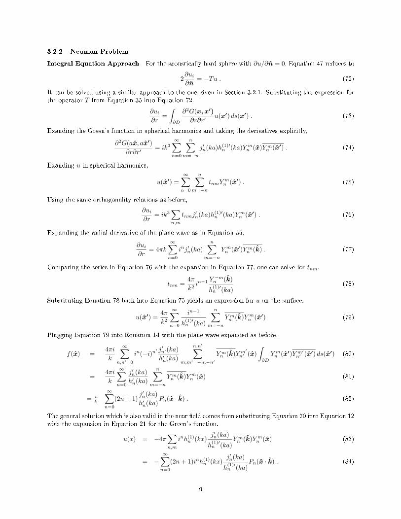
3.2.2 Neuman Problem

Integral Equation Approach For the acoustically hard sphere with ∂u/∂n = 0, Equation 47 reduces to

2∂ui

∂n= −Tu . (72)

It can be solved using a similar approach to the one given in Section 3.2.1. Substituting the expression forthe operator T from Equation 35 into Equation 72,

∂ui

∂r=

∫∂D

∂2G(x, x′)∂r∂r′

u(x′) ds(x′) . (73)

Exanding the Green's function in spherical harmonics and taking the derivatives explicitly,

∂2G(ax, ax′)∂r∂r′

= ik3∞∑

n=0

n∑m=−n

j′n(ka)h(1)′n (ka)Y m

n (x)Y mn (x′) . (74)

Exanding u in spherical harmonics,

u(x′) =∞∑

n=0

n∑m=−n

tnmY mn (x′) . (75)

Using the same orthogonality relations as before,

∂ui

∂r= ik3

∑n,m

tnmj′n(ka)h(1)′n (ka)Y m

n (x′) . (76)

Expanding the radial derivative of the plane wave as in Equation 55,

∂ui

∂r= 4πk

∞∑n=0

inj′n(ka)n∑

m=−n

Y mn (x′)Y m

n (k) . (77)

Comparing the series in Equation 76 with the expansion in Equation 77, one can solve for tnm.

tnm =4π

k2in−1 Y −m

n (k)

h(1)′n (ka)

(78)

Substituting Equation 78 back into Equation 75 yields an expression for u on the surface.

u(x′) =4π

k2

∞∑n=0

in−1

h(1)′n (ka)

n∑m=−n

Y mn (k)Y m

n (x′) (79)

Plugging Equation 79 into Equation 14 with the plane wave expanded as before,

f(x) =4πi

k

∞∑n,n′=0

in(−i)n′ j′n′(ka)h′n(ka)

n,n′∑m,m′=−n,−n′

Y mn (k)Y m′

n′ (x)∫

∂D

Y mn (x′)Y m′

n′ (x′) ds(x′) (80)

=4πi

k

∞∑n=0

j′n(ka)h′n(ka)

n∑m=−n

Y mn (k)Y m

n (x) (81)

= ik

∞∑n=0

(2n + 1)j′n(ka)h′n(ka)

Pn(x · k) . (82)

The general solution which is also valid in the near eld comes from substituting Equation 79 into Equation 12with the expansion in Equation 21 for the Green's function.

u(x) = −4π∑n,m

inh(1)n (kx)

j′n(ka)

h(1)′n (ka)

Y mn (k)Y m

n (x) (83)

= −∞∑

n=0

(2n + 1)inh(1)n (kx)

j′n(ka)

h(1)′n (ka)

Pn(x · k) . (84)

9

Series Approach As the the soft sphere, the hard sphere problem can be solved by requiring that thesum of the series for the normal derivative of the incident and scattered waves by zero.

∂

∂nui = − ∂

∂x′eik·ax′

= −4πk∑n,m

inj′n(ka)Y mn (x′)Y m

n (k) (85)

− ∂

∂nus =

∂

∂x′

∑n,m

anmh(1)n (kx′)Y m

n (x′) (86)

= k∑n,m

anmh(1)′n (ka)Y m

n (x′) (87)

anm = −4πinj′n(ka)

h(1)′n (ka)

h(1)n Y m

n (k) (88)

us(x) = −4π∑n,m

inh(1)n (kx)

j′n(ka)

h(1)′n (ka)

Y mn (k)Y m

n (x) (89)

= −∞∑

n=0

(2n + 1)inh(1)n (kx)

j′n(ka)

h(1)′n (ka)

Pn(x · k) (90)

3.2.3 Penetrable Scatterer

Integral Equation Approach The penetrable sphere can be computed with the series approach just aswas done with the soft and hard spheres. Because of the orthogonality of the spherical harmonics, it leadsto the same solution as the direct series solution which is outlined below. Since the extra algebra does littleto enlighten the reader about the characteristics of the solution, it will be omitted here.

Series Approach I will break the eld u at the boundary into three components: ui (the initial planewave), us (the scattered wave), and ud (the wave inside the scatterer). Expressing each of these as a seriesas before,

ui = 4π∑n,m

injn(ka)Y mn (x′)Y m

n (k) (91)

us =∑n,m

anmh(1)n (ka)Y m

n (x′) (92)

ud =∑n,m

bnmjn(kda)Y mn (x′) . (93)

Neglecting the pressure dierence enabled by the balloon (imagine scattering from bubbles in water, forinstance),

ui + us = ud . (94)

We can recover our acoustically soft sphere solution by setting bnm = 0. Since each term in the sum mulipliesby the same factor of Y m

n (x′), each term must be equal to zero.

4πinjn(ka)Y mn (k) + anmh(1)

n (ka)− bnmjn(kda) = 0 (95)

4πinjn(ka)Y mn (k) + anmh

(1)n (ka)

jn(kda)= bnm (96)

With our without the balloon, the radial velocities must match at the boundary as well (Equation 8).

1ρ

∂

∂x′(ui + us) =

1ρd

∂

∂x′ud (97)

10

Setting the sum of the derivative terms equal to zero yields

4πk

ρinj′n(ka)Y m

n (k) +k

ρanmh(1)′

n (ka) =kd

ρdbnmj′n(kda) (98)

4πkρ inj′n(ka)Y m

n (k) + kρanmh

(1)′n (ka)

kd

ρdj′n(kda)

= bnm . (99)

Setting the expression for bnm in Equation 96 equal to the expression for bnm in Equation 99,

4πinjn(ka)Y mn (k) + anmh

(1)n (ka)

jn(kda)=

4πkρdinj′n(ka)Y m

n (k) + kρdanmh(1)′n (ka)

kdρj′n(kda)

anm

[h

(1)n (ka)

jn(kda)− kρdh

(1)′n (ka)

kdρj′n(kda)

]= 4πinY m

n (k)[

kρdj′n(ka)

kdρj′n(kda)− jn(ka)

jn(kda)

]anm = 4πinY m

n (k)jn(kda)kρdj

′n(ka)− kdρj′n(kda)jn(ka)

kdρj′n(kda)h(1)n (ka)− jn(kda)kρdh

(1)′n (ka)

. (100)

Plugging Equation 100 into Equation 92 (with a going to x),

us(x) = 4π∑n,m

injn(kda)kρdj

′n(ka)− kdρj′n(kda)jn(ka)

kdρj′n(kda)h(1)n (ka)− jn(kda)kρdh

(1)′n (ka)

h(1)n (kx)Y m

n (k)Y mn (x) (101)

=∑

n

in(2n + 1)kρdj

′n(ka)jn(kda)− kdρj′n(kda)jn(ka)

kdρj′n(kda)h(1)n (ka)− kρdh

(1)′n (ka)jn(kda)

h(1)n (kx)Pn(k · x) (102)

f(x′) = − i

k

∑n

(2n + 1)kρdj

′n(ka)jn(kda)− kdρj′n(kda)jn(ka)

kdρj′n(kda)h(1)n (ka)− kρdh

(1)′n (ka)jn(kda)

Pn(k · x) . (103)

Note that if k = kd and ρ = ρd, the scattered wave has an amplitude of zero as would be expected. In thelimit of kd small, Equation 102 reduces to that for scttering from a hard sphere. In the limit of kd large,Equation 102 reduces to that for scattering from a soft sphere.

4 Balloon Scattering

In this section, I'll generalize the results from Section 3 to that from an idealized balloon. To make general-izations of this calculations explicit, I'll start by outlining the assumptions of the theory in this section.

1. The balloon is a perfect sphere.

2. The balloon membrane is neglibily thin and has the sole eect of providing a pressure dierence betweenthe gas on the outside of the balloon and inside the balloon.

3. The gasses inside and outside the balloon have uniform density and temperature.

5 Results

In this section, I have included some numerical results for the formas derived in this paper. They are dividedinto three groups, the acoustically soft sphere, the acoustically hard sphere, and penetrable scatterers.

5.1 Soft Sphere

The following Matlab functions were used to plot scattering from a soft sphere of radius a. The rst thingI needed were some short functions to computer spherical Bessel functions. The function in the sphj.m

computes the spherical Bessel function of the rst kind

jn(x) =√

π

2xJn+1/2(x) . (104)

11

function j=sphj(n,x)

% compute the spherical bessel function of the first kind

% of order n at the point x

j=sqrt(pi/(2*x))*besselj(n+0.5,x);

end

Similarly, the le function in sphh.m computes the spherical Hankel function of the rst kind

hn(x) =√

π

2xHn+1/2(x) . (105)

function h=sphh(n,x)

% compute the spherical hankel function of the first kind

% of order n at the point x

h=sqrt(pi/(2*x))*besselh(n+0.5,x);

end

5.1.1 Far Field

The function soft.m computes the cross section |f |2for a soft sphere of radius a (measured in wavelengths).

function [theta,intensity]=soft(a)

% *** soft(a) ***

% compute scattering from a soft sphere of radius a

% at the angle theta using nmax as the maximum value

% of n in the sum.

% The terms in the series oscillate up to about n=ka and then

% decrease rapidly. Taking 2ka terms, should be more than sufficient

% for large spheres. It always uses a minimum of 5 terms.

theta=0:0.01:pi; % scattering angle in radians

k=2*pi; % wave number with wavelength of 1

nmax=2*k*a+5;

nary=0:nmax;

nterm=2*nary+1;

jn=sphj(nary,k*a);

hn=sphh(nary,k*a);

% legendre calculates the associated legendre polynomials.

% I'm only interested in the m=0 one

for term=nary

lpn=legendre(term,cos(theta));

pn(term+1,:)=lpn(1,:);

end

for term=1:size(theta,2)

intensity(term)=abs(i/k*sum(nterm.*jn./hn.*pn(:,term)'))^2;

end

end

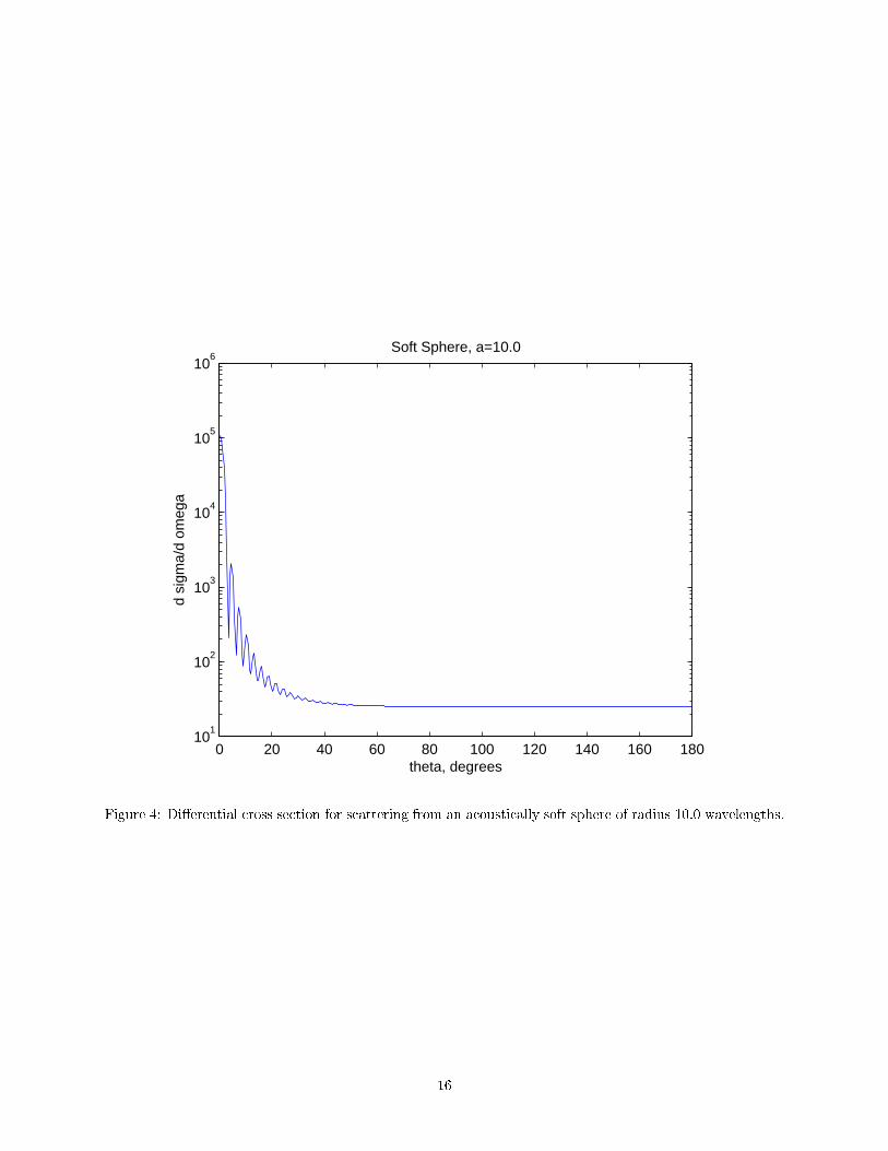
It is somewhat slow to run this program in Matlab for large spheres, but works ne for spheres up to 10wavelengths or so. Figures 1 through 4 are the squares of the scattering amplitude for acoustically softspheres of various wavelengths.

These plots generally look okay to me, but I'm worried about a factor of 2 in the normalization. For alarge sphere, I would expect the total cross section

σ =∫|f(Ω2 dΩ (106)

12

0 20 40 60 80 100 120 140 160 1800.004

0.006

0.008

0.01

0.012

0.014

0.016

theta, degrees

d si

gma/

d om

ega

Soft Sphere, a=0.1

Figure 1: Dierential cross section for scattering from an acoustically soft sphere of radius 0.1 wavelengths.

13

0 20 40 60 80 100 120 140 160 1800

2

4

6

8

10

12

14

16

18

20

theta, degrees

d si

gma/

d om

ega

Soft Sphere, a=1.0

Figure 2: Dierential cross section for scattering from an acoustically soft sphere of radius 1.0 wavelength.

14

0 20 40 60 80 100 120 140 160 18010

0

101

102

103

104

theta, degrees

d si

gma/

d om

ega

Soft Sphere, a=3.0

Figure 3: Dierential cross section for scattering from an acoustically soft sphere of radius 3.0 wavelengths.

15

0 20 40 60 80 100 120 140 160 18010

1

102

103

104

105

106

theta, degrees

d si

gma/

d om

ega

Soft Sphere, a=10.0

Figure 4: Dierential cross section for scattering from an acoustically soft sphere of radius 10.0 wavelengths.

16

to be equal to the cross sectional area of the sphere

A = πa2 . (107)

If I integrate |2/π numerically for spheres of radius 10 and 20, I get 10.282 and 20.022.

> > [theta10,dsigma10]=soft(10);

> > [theta20,dsigma20]=soft(20);

> > sqrt(sum(dsigma10.*sin(theta10))*(theta(2)-theta(1)))

ans =

10.2574

> > sqrt(sum(dsigma20.*sin(theta20))*(theta(2)-theta(1)))

ans =

20.0186

I can also do these integrals analytically by taking the large argument expansions for the Bessel and Hankel

functions. Abramowitz and Stegun[5] formula 10.1.16 gives a series expansion for h(1)n (z) as

h(1)n (z) = i−n−1z−1eiz

n∑k=0

(n + 1/2, k)(−2iz)−k . (108)

For large x, the dominant term in this series will be the k=0 term. Therefore, the asymptotic values for jn

and h(1)n for large x are

hn(x) =ei(x−π/2−nπ/2)

x(109)

jn(x) =cos

(x− π

2 −nπ2

)x

. (110)

Note that the asymptotic expansion for hn in Equation 109 can be subsituted into Equation 63 to giveEquation 66 and into Equation 82 to give Equation 84, providing a good cross check on those sets offormulas.

The integrated cross section can be computed using the orthogonality relation for the Legendre polyno-mials ∫ 1

−1

Pn(x)Pm(x) =2

2n + 1δn,m . (111)

The integrated square of Equation 66 is then

σ =∫

dσ

dΩdΩ =

∫|f |2 dΩ =

2k2

∞∑n=0

(2n + 1)(jn(ka))2∣∣∣h(1)

n (ka)∣∣∣2 . (112)

I'd like to make a further reduction of this analytically, but haven't been able to gure it out yet.

5.1.2 Near Field

I also implemented a computation of the near eld intensity in the le softnear.m. It takes a very longtime to run in matlab and is much more practical in a compiled language.

function [x,y,intensity]=softnear(a)

% *** soft(a) ***

% compute scattering from a soft sphere of radius a

% at the angle theta using nmax as the maximum value

% of n in the sum.

% The terms in the series oscillate up to about n=ka and then

% decrease rapidly. Taking 2ka terms, should be more than sufficient.

17

% It always uses a minimum of 5 terms.

x=-10:.1:10;

y=x;

k=2*pi; % wave number with wavelength of 1

nmax=2*k*a+5;

nary=0:nmax;

nterm=2*nary+1;

jn=sphj(nary,k*a);

hn=sphh(nary,k*a);

% legendre calculates the associated legendre polynomials.

% I'm only interested in the m=0 one

for ix=1:size(x,2)

for iy=1:size(y,2)

r=sqrt(x(ix)^2+y(iy)^2);

if(r<a)

intensity(ix,iy)=0;

else

for term=nary

lpn=legendre(term,x(ix)/r);

pn(term+1,:)=lpn(1,:);

end

hnx=sphh(nary,k*r);

intensity(iy,ix)=abs(exp(i*k*x(ix))-...

sum(i.^nary.*nterm.*jn./hn.*hnx.*pn'))^2;

end

end

end

end

Figure 5 is the output of an equivalent FORTRAN program for the total near eld intensity near a softsphere of radius 2.5 wavelengths.

5.2 Hard Sphere

The formulas for the hard sphere involve derivatives of bessel functions. These were computed using thedierentiation formula 10.1.22 in Abramowitz and Stegun[5],

d

dzfn(z) =

n

zfn(z)− fn+1(z) , (113)

where the function f can be jn, yn, or hn. The function sphjp computes d/dx fn(x).

function jp=sphjp(n,x)

% compute the derivative of the spherical bessel function of the

% first kind of order n at the point x

jp=n/x.*sphj(n,x)-sphj(n+1,x);

end

The function sphhp compute d/dx(1)n (x).

function hp=sphhp(n,x)

% compute the derivative of the spherical hankel function of the

% first kind of order n at the point x

hp=n/x*sphh(n,x)-sphh(n+1,x);

end

18

Figure 5: Near eld intensity for scattering from a soft sphere of radius 2.5 wavelengths.

19

5.2.1 Far Field

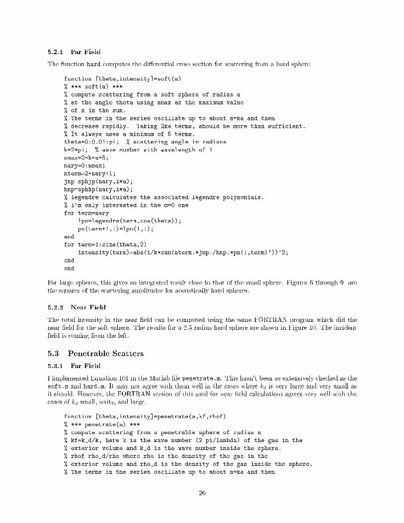
The function hard computes the dierential cross section for scattering from a hard sphere.

function [theta,intensity]=soft(a)

% *** soft(a) ***

% compute scattering from a soft sphere of radius a

% at the angle theta using nmax as the maximum value

% of n in the sum.

% The terms in the series oscillate up to about n=ka and then

% decrease rapidly. Taking 2ka terms, should be more than sufficient.

% It always uses a minimum of 5 terms.

theta=0:0.01:pi; % scattering angle in radians

k=2*pi; % wave number with wavelength of 1

nmax=2*k*a+5;

nary=0:nmax;

nterm=2*nary+1;

jnp=sphjp(nary,k*a);

hnp=sphhp(nary,k*a);

% legendre calculates the associated legendre polynomials.

% I'm only interested in the m=0 one

for term=nary

lpn=legendre(term,cos(theta));

pn(term+1,:)=lpn(1,:);

end

for term=1:size(theta,2)

intensity(term)=abs(i/k*sum(nterm.*jnp./hnp.*pn(:,term)'))^2;

end

end

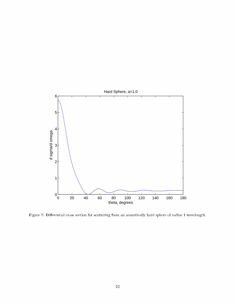
For large spheres, this gives an integrated result close to that of the small sphere. Figures 6 through 9 arethe squares of the scattering amplitudes for acoustically hard spheres.

5.2.2 Near Field

The total intensity in the near eld can be computed using the same FORTRAN program which did thenear eld for the soft sphere. The results for a 2.5 radius hard sphere are shown in Figure 10. The incidenteld is coming from the left.

5.3 Penetrable Scatters

5.3.1 Far Field

I implemented Equation 101 in the Matlab le penetrate.m. This hasn't been as extensively checked as thesoft.m and hard.m. It may not agree with them well in the cases where kd is very large and very small asit should. However, the FORTRAN version of this used for near eld calculations agrees very well with thecases of kd small, unity, and large.

function [theta,intensity]=penetrate(a,kf,rhof)

% *** penetrate(a) ***

% compute scattering from a penetrable sphere of radius a

% kf=k_d/k, here k is the wave number (2 pi/lambda) of the gas in the

% exterior volume and k_d is the wave number inside the sphere.

% rhof=rho_d/rho where rho is the density of the gas in the

% exterior volume and rho_d is the density of the gas inside the sphere.

% The terms in the series oscillate up to about n=ka and then

20

0 20 40 60 80 100 120 140 160 1800

1

2

3

4

5

6

7

8x 10

−4

theta, degrees

d si

gma/

d om

ega

Hard Sphere, a=0.1

Figure 6: Dierential cross section for scattering from an acoustically hard sphere of radius 0.1 wavelengths.

21

0 20 40 60 80 100 120 140 160 1800

1

2

3

4

5

6

theta, degrees

d si

gma/

d om

ega

Hard Sphere, a=1.0

Figure 7: Dierential cross section for scattering from an acoustically hard sphere of radius 1 wavelength.

22

0 20 40 60 80 100 120 140 160 18010

−2

10−1

100

101

102

103

theta, degrees

d si

gma/

d om

ega

Hard Sphere, a=3.0

Figure 8: Dierential cross section for scattering from an acoustically hard sphere of radius 3 wavelengths.

23

0 20 40 60 80 100 120 140 160 18010

0

101

102

103

104

105

theta, degrees

d si

gma/

d om

ega

Hard Sphere, a=10.0

Figure 9: Dierential cross section for scattering from an acoustically hard sphere of radius 10 wavelengths.

24

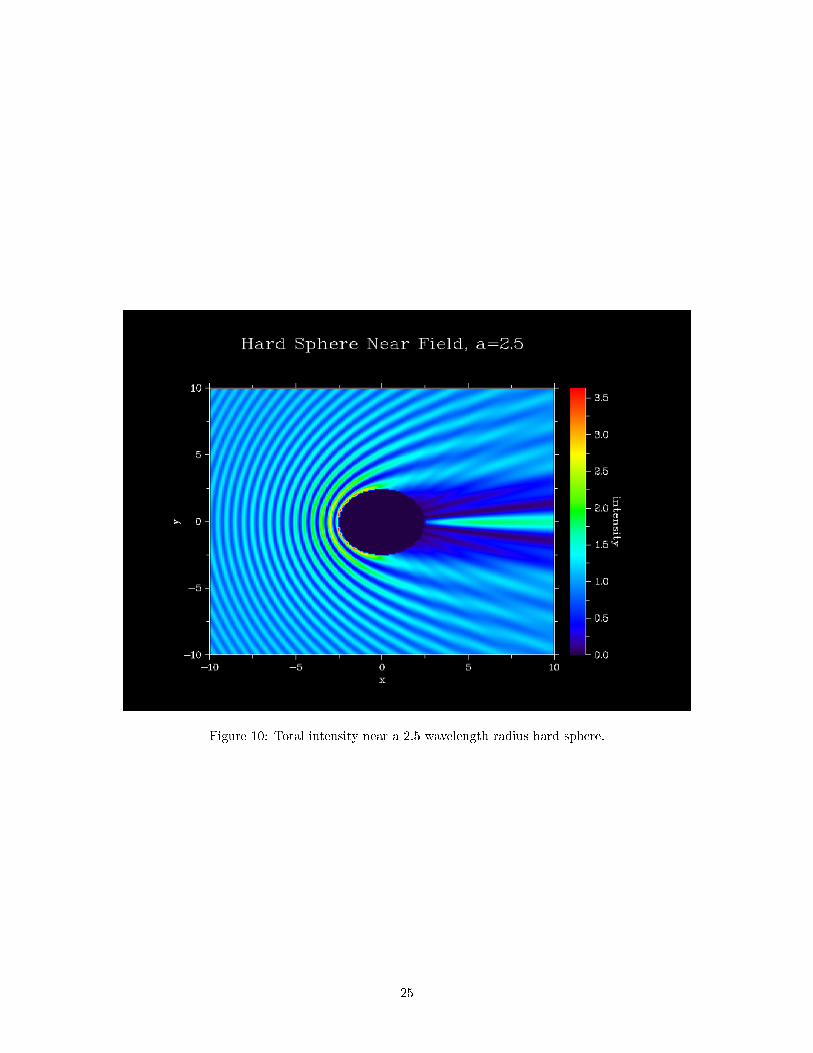
Figure 10: Total intensity near a 2.5 wavelength radius hard sphere.

25

% decrease rapidly. Taking 2ka terms, should be more than sufficient.

% It always uses a minimum of 5 terms.

theta=0:0.01:pi; % scattering angle in radians

k=2*pi; % wave number with wavelength of 1

ka=k*a;

kda=k*kf*a;

nmax=2*k*a+5;

nary=0:nmax;

nterm=2*nary+1;

jn=sphj(nary,ka);

hn=sphh(nary,ka);

jnp=sphjp(nary,ka);

hnp=sphhp(nary,ka);

jnd=sphj(nary,kda);

jnpd=sphjp(nary,kda);

% legendre calculates the associated legendre polynomials.

% I'm only interested in the m=0 one

for term=nary

lpn=legendre(term,cos(theta));

pn(term+1,:)=lpn(1,:);

end

for term=1:size(theta,2)

num=rhof*jnp.*jnd-kf*jnpd.*jn;

denom=kf*jnpd.*hn-rhof*hnp.*jnd;

intensity(term)=abs(-i/k*sum(nterm.*num./denom.*pn(:,term)'))^2;

end

end

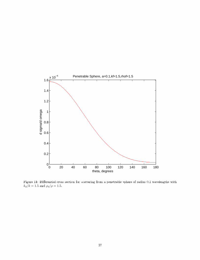
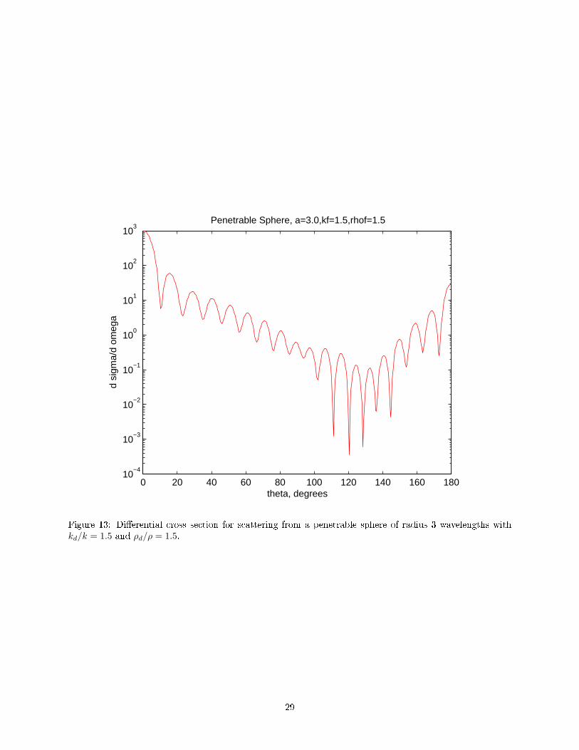
Figures 11 through 14 are the squares of the scattering amplitudes for penetrable spheres.

5.3.2 Near Field

The same FORTRAN program used to compute near eld intenisities for the hard and soft spheres was alsoused with a penetrable sphere. Figure 15 shows the results of running this program for a sphere is radius 2.5wavelengths with k_d=1.2 and \rho_d=1.2. An interesting feature is the focussing of the incident beamwith a maximum intensity about 4 wavelengths beyond the center of the sphere.

5.4 Balloon

References

[1] S. Turley, Scattering from a Circle, Internal Hughes Research Laboratory Notes, Aug. 1992.

[2] S. Turley, 2d Scalar Surface Scattering, Internal Hughes Research Laboratory Notes, May 1992.

[3] R. Kress, Acoustic Scattering, in Scattering - Scattering and Inverse Scattering in Pure and Applied

Science, edited by E. Pike and P. Sabatier, chapter 2, Academic Press, London, 2001.

[4] R. Kress, Acoustic Scattering, November 2006, a copy of sections 2.1 and 2.2 can be found athttp://diogenes.iwt.uni-bremen.de/vt/laser/papers/Kress-acustic-scatter-ed-book.ps.

[5] M. Abramowitz and I. A. Stegun, Handbook of Mathematical Functions, Applied Mathematics Series,National Bureau of Standards, Cambridge, 1972.

26

0 20 40 60 80 100 120 140 160 1800

0.2

0.4

0.6

0.8

1

1.2

1.4

1.6x 10

−4

theta, degrees

d si

gma/

d om

ega

Penetrable Sphere, a=0.1,kf=1.5,rhof=1.5

Figure 11: Dierential cross section for scattering from a penetrable sphere of radius 0.1 wavelengths withkd/k = 1.5 and ρd/ρ = 1.5.

27

0 20 40 60 80 100 120 140 160 1800

2

4

6

8

10

12

14

16

18

20

theta, degrees

d si

gma/

d om

ega

Penetrable Sphere, a=1.0,kf=1.5,rhof=1.5

Figure 12: Dierential cross section for scattering from a penetrable sphere of radius 1 wavelength withkd/k = 1.5 and ρd/ρ = 1.5.

28

0 20 40 60 80 100 120 140 160 18010

−4

10−3

10−2

10−1

100

101

102

103

theta, degrees

d si

gma/

d om

ega

Penetrable Sphere, a=3.0,kf=1.5,rhof=1.5

Figure 13: Dierential cross section for scattering from a penetrable sphere of radius 3 wavelengths withkd/k = 1.5 and ρd/ρ = 1.5.

29

0 20 40 60 80 100 120 140 160 18010

−2

10−1

100

101

102

103

104

105

106

theta, degrees

d si

gma/

d om

ega

Penetrable Sphere, a=10.0,kf=1.5,rhof=1.5

Figure 14: Dierential cross section for scattering from a penetrable sphere of radius 10 wavelengths withkd/k = 1.5 and ρd/ρ = 1.5.

30

Figure 15: Total near eld for scattering from a penetrable sphere of radius 2.5 wavelengths and with kd = 1.2and ρd = 1.2.

31