
ACOUSTIC EMISSION FOR FATIGUE CRACK MONITORING …orca.cf.ac.uk/47735/2/2013MohdSPhD.pdf ·...
179
i ACOUSTIC EMISSION FOR FATIGUE CRACK MONITORING IN NUCLEAR PIPING SYSTEM PhD Thesis Shukri Mohd Cardiff School of Engineering Cardiff University, Cardiff UK 2012
Transcript of ACOUSTIC EMISSION FOR FATIGUE CRACK MONITORING …orca.cf.ac.uk/47735/2/2013MohdSPhD.pdf ·...
i
ACOUSTIC EMISSION FOR FATIGUE CRACK MONITORING IN
NUCLEAR PIPING SYSTEM
PhD Thesis
Shukri Mohd
Cardiff School of Engineering
Cardiff University, Cardiff
UK
2012
ii
SUMMARY OF THESIS
Candidate’s Name: Shukri Mohd
Candidate’s for the Degree of: PHD
Institution at which study pursued: School of Engineering, Cardiff University
Full title of Thesis: Acoustic Emission for Fatigue Crack Monitoring in Nuclear Piping
System
Summary:
Accurate Acoustic Emission (AE) source location is crucial for monitoring the thermal
fatigue crack in nuclear piping systems. Conventional Time of Arrival (TOA) location
techniques can provide estimated location of fatigue cracks but are not accurate enough
to allow crack size estimation. This thesis examines the role of AE as a Non-destructive
Testing (NDT) tool for thermal fatigue damage monitoring in nuclear piping system.
The work focuses on developing an accurate AE source location technique. The works
is divided into three main areas of research:
1. Development of Wavelet Transform analysis and Modal Location (WTML)
method
A novel location method was successfully developed using modal location theory and
wavelet transform analysis. Source location was performed on a steel plate of 790 x 300
mm with nominal thickness of 5 mm under a planar location setup using H-N sources.
The accuracy of the new technique was compared with the major location methods (the
time of arrival (TOA) technique, triple point filtering and DeltaT location methods). The
result of the study shows that the WTML method produces more accurate location result
compared with other AE location methods.
2. Validation of WTML method for accurate location of fatigue crack growth in
steel plate
Laboratory fatigue tests were conducted on steel plate in order to monitor and locate
fatigue crack growth, and validate the workability of WTML method. WTML was
successful in locating the AE signal released from fatigue crack growth. The accuracy
of WTML is much better than TOA, DeltaT and triple point filtering location methods.
3. Crack size measurement using WTML method
The capability of the WTML location method to measure crack length due to fatigue
crack growth under tensile-tensile loading is investigated. The WTML method
successfully used to determine the crack length in the steel pipe with the maximum
measurement error of 5 mm.
Key Words: Acoustic Emission, Damage detection, Fatigue Crack Growth, Source
location, Modal Analysis, Wavelet Transform Analysis, Crack-length measurement

iii
ACKNOWLEDGEMENTS
Praise to God, The Almighty, who gave me this opportunity to complete this research
work.
I take this opportunity to express my deep gratitude to Prof. K. Holford for her great
supervision throughout my study. Her guidance and encouragement are much
appreciated. I am also grateful to Dr. Rhys Pullin for his excellent guidance and support
throughout this study.
My thanks also to all Acoustic Emission (AE) group members especially Dr. Mark
Eaton, Matthew Pearson and Hisyam for their technical advice and help. Many thanks
to all staff of the Cardiff University Mechanical and Structural Engineering Divisions;
particularly Harry Lane, Len Czekaj, Des Sanford and Brian Hooper for their
continuous support during my experimental work.
Finally I extend my deepest thanks to my dearest wife Juliawati and my lovely daughter
Nurul Afifah and all of my family members for their patient and support throughout my
study.
iv
GLOSSARY OF TERM
Acoustic Emission:
Acoustic Emission Signal: The electrical signal obtained by an instrumented computer
system through the detection of Acoustic Emission
Hit: A hit is the term used to indicate that a given AE channel has detected and
processed an acoustic emission transient.
Event: A single AE source produces a transient mechanical wave that propagates in all
direction in medium. The AE wave is detected in the form of hits on one or more
channels. An event therefore, is a group of AE hits that was received from a single
source.
Source: Place where the event takes place.
Noise: The signal obtained in the absence of any acoustic emission.
Sensor: Device that converts the physical parameter of wave into an electrical
parameter.
Resonant Sensor: High sensitivity over a narrow frequency band.
Wideband Sensors: High sensitivity over a large frequency band.
Source location: Computed origin of the acoustic source.
Location Plot: Representation of sources of acoustic emission computed using an array
of sensors.

v
INDEX OF CONTENTS
SUMMARY OF THESIS i
ACKNOWLEDGEMENTS ii
LIST OF FIGURES iii
LIST OF TABLES viii
GLOSSARY OF TERMS ix
CHAPTER 1: INTRODUCTION
1.1 Structural Integrity of Nuclear Piping 1
1.2 NDT and Structural Integrity 3
1.3 Research Objective 4
1.4 Major contribution of research work 4
1.5 Publication of research outcomes 5
1.6 Outline of thesis 5
CHAPTER 2: BACKGROUND AND THEORY
2.1 Introduction 7
2.2 Acoustic Emission (AE) 7
2.2.1 Introduction 7
2.2.2 Signal measurement parameters 8
2.2.3 AE sources mechanism 11
2.2.4 AE wave propagation 13
2.2.5 Wave attenuation 16
2.3 Modal analysis 17
2.3.1 Modal Acoustic Emission 18
2.3.2 Dispersion curve 20
2.3.3 Modified dispersion curve 20
2.4 AE source location 21
2.4.1 Introduction 21
2.4.2 Time of Arrival (TOA) source location 22
2.4.3 DeltaT location 26
2.4.4 Waveform filtering based source location 28
vi
2.4.5 Single Sensor Modal Analysis Location 29
2.5 Wavelet Transform 30
2.5.1 Introduction to AE signal analysis 30
2.5.2 Fundamental of wavelet transform 31
2.5.3 Source location of Lamb waves AE signals by wavelet transform 32
2.5.4 Signal denoising of AE using Discrete Wavelet Transform (DWT) 34
2.5.5 Signal characterization using wavelet transform analysis 35
2.6 Thermal fatigue 35
2.6.1 Introduction to fatigue 35
2.6.2 Thermal fatigue in nuclear piping 37
2.6.3 Fatigue and AE 40
2.7 Conclusions 42
CHAPTER 3: EXPERIMENTAL EQUIPMENT AND TECHNIQUES
3.1 AE instrumentation and software 45
3.1.1 Data acquisition and storage 45
3.1.2 AE sensors 46
3.1.3 AE preamplifier 51
3.1.4 Hsu-Nielsen source 52
3.1.5 Couplant 54
3.1.6 Sensor mounting 55
3.2 Data replay and analysis 57
3.2.1 Graphical representation 57
3.2.2 Wavelet transform analysis 60
3.3 Fatigue loading and crack monitoring 64
3.3.1 Loading machine 64
3.3.2 Linear variable differential transducer 64
3.3.3 Crack gauge 65
3.4 Experimental techniques gauge measurement 67
3.4.1 AE sensor mounting and sensitivity verification 67
3.4.2 Wave velocity determination 69
3.4.3 Crack length measurement 69
3.4.4 Dye penetrant inspection 70
3.4.5 DeltaT source location 71
vii
3.4.6 Triple point filtering analysis 72
3.5 Summary 72
CHAPTER 4: Development of Novel Wavelet Transform Analysis and Modal Location
(WTML) Methodology
4.1 Introduction 74
4.2 AE source location technique ; principal and limitation 74
4.2.1 Time of arrival (TOA) 74
4.2.2 DeltaT 75
4.2.3 Single sensor modal analysis location (SSMAL) 76
4.3 SSMAL with Modified Dispersion Curve 76
4.3.1 Introduction 76
4.3.2 Objective of the study 77
4.3.3 Experimental procedure 77
4.3.4 Dispersion curve analysis 78
4.3.5 Preliminary SSMAL 80
4.3.6 Modified dispersion work and analysis 82
4.3.7 Summary of finding from modified dispersion work and analysis 85
4.4 Proposed wavelet transform analysis and modal location (WTML)
methodology 86
4.4.1 Introduction 86
4.4.2 WTML approach 87
4.5 Wavelet Transform Analysis and Modal Location (WTML) of Artificial
Sources in A Steel Plate 89
4.5.1 Experimental Setup and Validation Procedure 89
4.5.2 Results and discussion 90
4.5.3 Summary of finding 95
4.6 Wavelet Transform Modal Location (WTML) of Artificial Sources in A Steel
Pipe Section 96
4.6.1 Experimental Setup and Validation Procedure 96
4.6.2 Results and Discussion 98
4.6.3 Summary of finding 102
4.7 Conclusions and future work 103
viii
CHAPTER 5: ACOUSTIC EMISSION CRACK LENGTH MEASUREMENT IN
STEEL PLATE AND PIPE USING A WAVELET TRANSFORM
ANALYSIS AND MODAL LOCATION THEORY
5.1 Introduction 102
5.2 AE from fatigue crack in pipe 102
5.2.1 Specimen geometry 102
5.2.2 Experimental procedure and signal analysis 103
5.2.3 Results and discussion 105
5.2.4 Conclusion for AE source location in steel pipe 119
5.3 Crack length measurement in steel plate using WTML 120
5.3.1 Specimen geometry 120
5.3.2 Experimental equipment, procedure and analytical method 122
5.3.3 Results and discussion 129
5.4 Summary of findings 151
CHAPTER 6: CONCLUSION AND FUTURE WORK 153
6.1 Summary of conclusions 153
6.2 Recommendation for further work 156
CHAPTER 7: REFERENSES 158
Appendix A 167
Appendix B 171
1
CHAPTER 1: INTRODUCTION
This chapter begins with relevant background information regarding structural
integrity of nuclear piping (Section 1.1), followed by a brief explanation on
Acoustic Emission (AE) and other non-destructive testing (NDT) techniques as
structural integrity monitoring tools, their strengths and limitations (Section 1.2).
The objective and scope of the research work is explained in Section 1.3 while
Section 1.4 details the major contributions of this work. Finally, Section 1.5
presents an outline of the remaining chapters of the thesis.
1.1 Structural integrity of nuclear piping
Piping integrity is a major issue for nuclear plant safety. Piping systems in nuclear
power plants are designed for pressures and mechanical loads originating from
deadweight and seismic events and operating thermal transients using the equations
in the ASME Boiler and Pressure Vessel Code, Section III (ASME, 2006).
In nuclear power plant, carbon steels and low alloy steels are usually used for
various pipe components. These structures are not only subjected to mechanical
loads, but are frequently exposed to aggressive thermal loads which induce the
formation of fatigue cracks especially in the welded area. Thermal fatigue can
occur in nuclear piping through a number of different mechanisms such as wall
thermal gradient stress, piping thermal expansion and thermal stratification stress.
Both thermal gradient stresses and thermal expansion is well considered in the
ASME codes design stress analysis, however thermal stratification is not
considered in this design code (Hirschberg, 2000).
Thermal fatigue cracks have been reported to occur in primary loop recirculation
pipes and various other components of nuclear power plants (Hayashi, 1998).
Thermal fatigue has also been identified as the major ageing mechanism of nuclear
piping system such as in piping connected to Reactor Coolant System (RCS)
especially for surge, spray and branch lines and their nozzles that are subject to
2
thermal transients during plant start-up and shut-down, thermal stratification,
thermal shock, turbulent penetration, and thermal cycling (EPRI, 2005).
Thermal stratification may also cause leaks in normally stagnant lines connected to
the reactor coolant loop in safety injection systems, reactor coolant drain lines, a
residual heat removal suction line, and an excess letdown line. In addition,
stratification has caused cracking of steam generator feed water nozzles and high
piping displacements in pressuriser surge lines (Bieniussa, 1999).Thermal fatigue
can lead to cracks formation and these cracks can be categorised as small leaks in
piping or medium leaks in piping when crack opening is more than 1 mm
(NEA/CSNI/R, 2005).
In normal practice, after detection of a fatigue crack during periodic non-destructive
inspection, fracture mechanics methodology is used to estimate the safe operational
life of the component or structure. Furthermore, a life prediction study can be
useful to determine component flaw inspection intervals along with critical flaw
shape and sizes for safety acceptance criteria. Based upon this information,
maintenance and replacement schedules can be planned to ensure continued safe
performance of the plant.
Section XI of ASME Boiler and Pressure Vessel Code provide the guidelines for
nuclear power industry to evaluate the serviceability of piping component that is
subject to cyclic stress such as thermal fatigue. One of the key parts of Section XI
of this code is a damage tolerance analysis which postulates the flaw at thermal
fatigue location and then performs thermal fatigue crack growth analysis to
determine the inspection intervals that can detect the fatigue cracks before they
exceed the critical size allowed by the governing code (Gosselin et. al., 2007).
Damage tolerance analysis of piping structural components is used to avoid
catastrophic failure and to maintain the safe and reliable operation of piping
structures especially for ageing nuclear power plants.
3
1.2 NDT and structural integrity monitoring
There is a comprehensive ageing management program in place for all the
operating nuclear power plants. Periodic in-service inspection of critical
components such piping system is very important for assuring their structural
integrity and the safe operation of nuclear power plants. Non-destructive testing
techniques play a crucial role in this regard and are conducted based on the
guideline of Section XI of ASME Boiler and Pressure Vessel Code.
Acoustic Emission (AE) is considered as a passive NDT technique because AE
detects emitted elastic waves within structure during deformation while most other
traditional NDT methods such as radiography, ultrasound and eddy currents require
a source input and are therefore defined as active testing technique. A major
strength of AE is its ability to be used as a “global” monitoring tool (Holford et al.
1999) i.e. it can provide inspection on a wider area compared with other NDT
techniques.
AE offers the opportunity to monitor the thermal fatigue damage continuously and
cracks can be identified at early initiation stage of formation without intrusion on
the test schedule. AE offers several advantages over other NDT techniques for
monitoring fatigue crack growth on piping structure such as nuclear piping system:-
It provides the ability to monitor the structure throughout the test period
without interruption.
It provides global monitoring of the structure.
It requires minimum accessibility.
It can provide an early warning before catastrophic failure, an option to stop
the test, improving safety and saving cost.
Conventional acoustic emission testing methods, however, suffer from some
draw- backs. Current AE location techniques only give estimated location of
fatigue crack growth area. The exact size of fatigue crack growth cannot be
determined using available commercial AE source location systems. The result of
AE tests are usually followed by other conventional NDT methods such
4
ultrasonic testing for determining the accurate location and size of damage for
further repairing processes.
1.3 Research objectives
The aim of this research work is to develop an accurate AE location technique for
use in the global and local monitoring of thermal fatigue crack in steel pipes, in
order to provide a commercial NDT tool for structural integrity monitoring of
nuclear piping systems.
The main objectives are to evaluate and enhance current methods for locating the
fatigue crack growth in the steel pipe member using standard artificial acoustic
emission sources and validated these techniques using actual AE data from fatigue
crack growth.
1.4 Major contribution of the research work
Major significant contribution of this research can be summarised as follows:
1. Development of novel AE location method based on wavelet transforms
analysis and modal location method applied to fatigue cracks. This method is
named ‘Wavelet Transform analysis and Modal Location’ (WTML). This
method is found to be more accurate than available commercial location
methods and comparable with advanced location methods such as the DeltaT
(Baxter 2007) technique. However, WTML method is superior to the DeltaT
method because it is easier to use and does not involve prior calibration. In
addition, the proposed method could be applied using only a single sensor.
2. Validation of new methods for locating the actual fatigue crack growth on
steel plate under cyclic tensile loading. The proposed method was successfully
used to accurately locate fatigue crack growth in steel plate.
3. Deployment of discrete wavelet transforms (DWT) de-noising methodology to
improve temporal measurement error in modal analysis. DWT de-noising
5
capability was found to significantly improve the accuracy of SSMAL for
locating actual fatigue crack growth signal that contained excessive back
ground noise.
1.5 Publication of research outcomes
The publications from this research are as follows:
Conference Papers
1. Shukri MOHD, Karen M. HOLFORD and Rhys PULLIN. “Acoustic
Emission Source Location in Steel Structures Using a Wavelet
Transform analysis and Modal Location Theory”. In 7th
International
Conference on Acoustic Emission Testing, Granada, September 2012.
2. Shukri MOHD, Karen M. HOLFORD and Rhys PULLIN. “Planar
Location of Simulated AE source on Steel Pipe using a Wavelet
Transform analysis based on Modal Location Theory”. International
Conference on Humanities, Social Science, Science and Technology,
Cardiff, July 2012
1.6 Outline of thesis
This chapter provides background information on thermal fatigue damage
monitoring in nuclear piping. The benefits of AE monitoring for this application
have been discussed and the objectives of this research have been identified.
Chapter Two presents relevant background information and theory. AE theory of
source mechanisms, wave propagation and source location is provided along with
wavelet transform analysis and thermal fatigue theory. A review of past failures in
nuclear piping due to thermal fatigue is also included.
6
Chapter Three discusses experimental equipment, procedure and techniques utilised
and developed throughout the research. This chapter also describes the software
used for analysis of the AE data from artificial and actual sources.
Chapter Four describes a novel method developed to improve source location in
plate like structure especially for nuclear power plant piping system based on
Modal AE (MAE) theory and wavelet transform analysis. H-N tests on plate and
pipe were completed to validate the method. The results are presented and
discussed.
Chapter Five describe a fatigue test on a notched plate under tension loading. This
test was carried out to validate the newly developed method to precisely locate the
AE signal from fatigue crack growth in a plate under cyclic tensile loading and
compare the location accuracy with other methods such as TOA planar location,
DeltaT location and waveform filtering. The accuracy of location is then validated
by a crack gauge measurement.
Chapter Six discusses a fatigue test on notched pipe under four point bend loading.
This test was carried out to validate the newly developed method to precisely
locating the AE signal from fatigue crack growth on a steel pipe. This chapter also
discussed the application of the DWT denoisiong methodology for remove noise
from the AE waveform and how this can then improve MAE source location for
actual fatigue signal.
Finally, Chapter Seven summarises the overall conclusions and findings of the
study and suggests directions for future research and development, and Chapter
Eight contains all the references to research cited in this thesis.
7
CHAPTER2: BACKGROUND AND THEORY
2.1 Introduction
This chapter presents relevant background information and theory on AE source
mechanisms, Lamb waves theory and wave propagation, and source location along
with wavelet transform analysis and thermal fatigue. A review of past failures in
nuclear piping due to thermal fatigue is also included.
2.2 Acoustic Emission (AE)
2.2.1 Background theory
AE is a transient elastic wave generated by the rapid release of energy from a
localised source within a material (ASTM 1982). AE is a natural phenomenon and
occurs in a wide range of materials, structures and processes. The largest-scale of
AE is seismic events, while the smallest-scale processes that have been observed
during AE tests are the movement of small numbers of dislocations in stressed
metals (Miller and McIntire 1987).
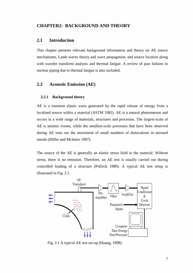
The source of the AE is generally an elastic stress field in the material. Without
stress, there is no emission. Therefore, an AE test is usually carried out during
controlled loading of a structure (Pollock 1989). A typical AE test setup is
illustrated in Fig. 2.1.
Fig. 2.1 A typical AE test set-up (Huang, 1998).
8
AE sensors mounted on the structure detect the displacement of the surface and
convert this tiny movement to an electrical signal by using a piezoelectric crystal.
After sensing and pre-amplification, the signal is transmitted to the main instrument,
where it is amplified and filtered.
Detection of the signal is accomplished with a comparator circuit, which generates
a digital output pulse whenever the AE signals exceeds a fixed threshold voltage.
The threshold level is usually set by the operator and is the key variable that
determines the test sensitivity (Miller and McIntire 2005).
AE equipment is highly sensitive to any kind of surface displacement within its
operating frequency range, typically 20 to 1200 kHz. The equipment can detect not
only crack growth and material deformation but also such processes as
solidification, flow and phase transformation (Miller and McIntire, 1987).
Due to recent advancement in acquisition speeds and processors, the latest AE
equipment is able to handle high rate data acquisition and faster signal processing.
AE equipment with large data storage has enabled waveform data to be stored by
the AE system which provide better understanding of AE wave propagation (Miller
and McIntire, 2005).
2.2.2 Signal measurement parameters
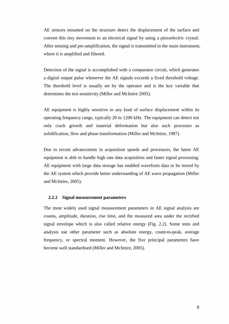
The most widely used signal measurement parameters in AE signal analysis are
counts, amplitude, duration, rise time, and the measured area under the rectified
signal envelope which is also called relative energy (Fig. 2.2). Some tests and
analysis use other parameter such as absolute energy, count-to-peak, average
frequency, or spectral moment. However, the five principal parameters have
become well standardised (Miller and McIntire, 2005).
9
Fig. 2.2 Definitions used for recording acoustic-emission events (Huang, 1998).
Amplitude, A, is the highest peak voltage attained by an AE waveform. This is very
important parameter because it directly determines the detectability of the AE event.
AE amplitudes are directly related to the magnitude of the source event, and they
vary over a wide range from micro-volts to volts. The amplitudes of AE are
customarily expressed on a decibel scale, in which 1 V at the transducer is defined
as 0 dB, 10 V as 20dB, 100 V as 40dB and so on.
Counts, N, are the threshold-crossing pulses and sometimes are called ring-down
counts. This is the one of the oldest and easiest ways to quantify the AE signal.
Counts depend strongly on the acoustic properties and reverberant nature of both
the specimen and sensor.
MARSE Energy, E, is the measured area under the rectified signal envelope. Energy
is preferred over counts because it is sensitive to amplitude as well as duration, and
it is less dependent on the threshold setting and operating frequency. True Energy,
is a measure of the AE hit and is measured in atto-joules (1x10⁻¹⁰
J = 1 aJ).
Absolute energy is derived from integral of the squared voltage signal divided by
reference resistance (10kΩ) over the duration of acoustic emission waveform
packet. This parameter represents the true energy of an AE event from transient
signals or of certain data rate interval of continuous AE signals (PAC 2005).
10
Duration, D, is the time from the first threshold crossing to the last. Duration is
measured in microseconds. It is valuable for noise filtering and other type of signal
qualification.
Rise time, R, is the elapsed time from the first threshold crossing to the signal peak.
In modern AE system, these parameters are known as feature data and are captured
by signal processing software by extracting the value of these parameters from
waveform data. This parameter can be used for several types of signal qualification
and noise rejection and is dependent on wave propagation processes between
source and sensor.
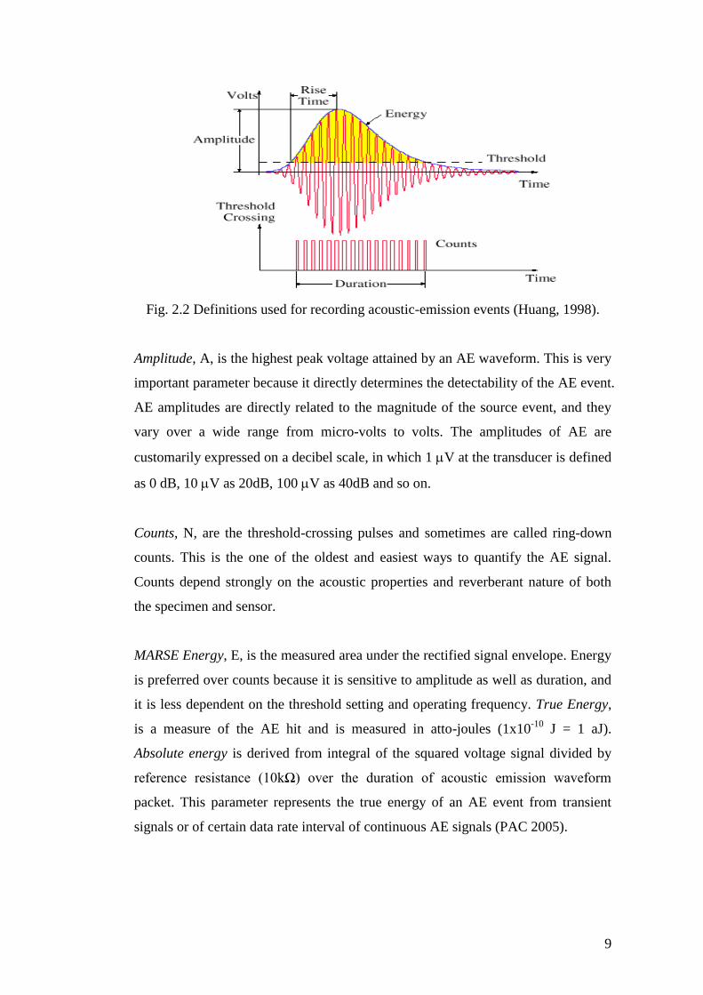
AE signals can be analysed by correlating one feature to the others or to other
parameters such as load, strain location or time. Fig. 2.3 below shows AE data
displays based on data feature correlation that are commonly used in AE signal
analysis.
Fig. 2.3 Typical AE data display for AE signal analysis based on signal feature
extraction (Baxter 2007)
11
A detailed explanation about AE data display was well explained by Pollock (1989)
and in general AE can be classed as:
History/Time plots
Distribution functions to show the statistical properties of the emission
Channel plots showing the distribution of detected emission by each channel
Location displays that shows the position of an AE source
Point plots showing the correlation different AE parameters and
Diagnostic plots showing the severity of AE indications from different parts
or locations of the structure
2.2.3 AE sources mechanism
AE are stress waves produced by rapid released of elastic energy in stressed
materials. Emission from these sources can be categorised as either transient or
continuous wave.
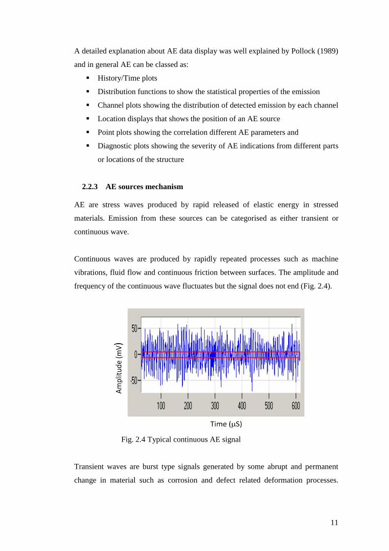
Continuous waves are produced by rapidly repeated processes such as machine
vibrations, fluid flow and continuous friction between surfaces. The amplitude and
frequency of the continuous wave fluctuates but the signal does not end (Fig. 2.4).
Fig. 2.4 Typical continuous AE signal
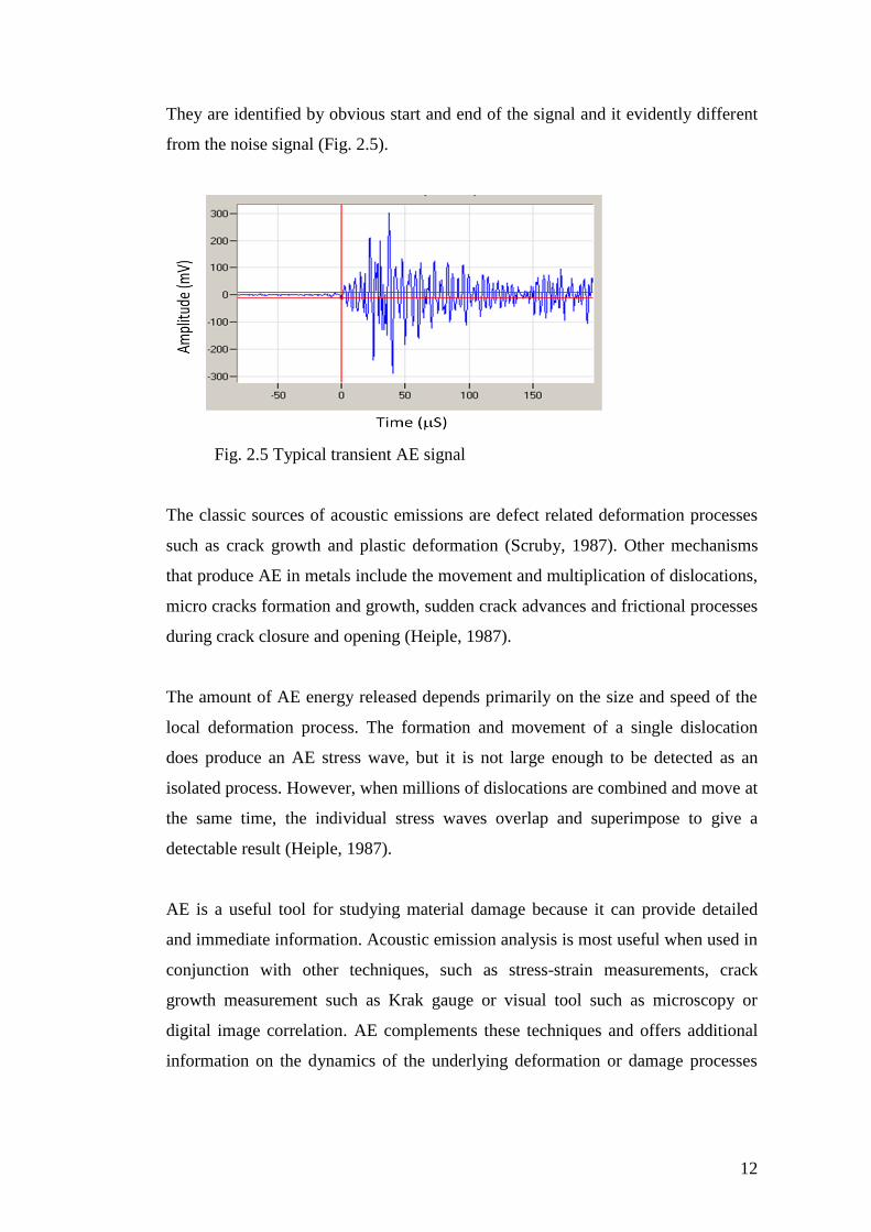
Transient waves are burst type signals generated by some abrupt and permanent
change in material such as corrosion and defect related deformation processes.
12
They are identified by obvious start and end of the signal and it evidently different
from the noise signal (Fig. 2.5).
Fig. 2.5 Typical transient AE signal
The classic sources of acoustic emissions are defect related deformation processes
such as crack growth and plastic deformation (Scruby, 1987). Other mechanisms
that produce AE in metals include the movement and multiplication of dislocations,
micro cracks formation and growth, sudden crack advances and frictional processes
during crack closure and opening (Heiple, 1987).
The amount of AE energy released depends primarily on the size and speed of the
local deformation process. The formation and movement of a single dislocation
does produce an AE stress wave, but it is not large enough to be detected as an
isolated process. However, when millions of dislocations are combined and move at
the same time, the individual stress waves overlap and superimpose to give a
detectable result (Heiple, 1987).
AE is a useful tool for studying material damage because it can provide detailed
and immediate information. Acoustic emission analysis is most useful when used in
conjunction with other techniques, such as stress-strain measurements, crack
growth measurement such as Krak gauge or visual tool such as microscopy or
digital image correlation. AE complements these techniques and offers additional
information on the dynamics of the underlying deformation or damage processes
13
and the transitions from one type of deformation or damage to another (Pollock,
1989).
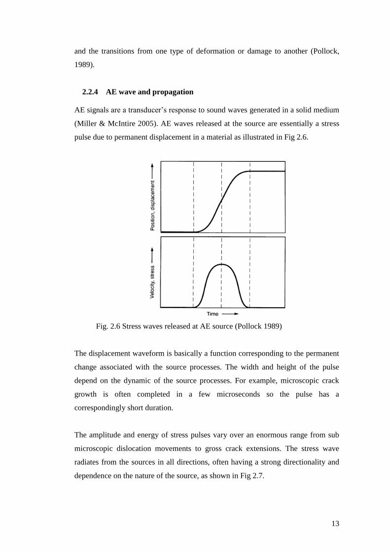
2.2.4 AE wave and propagation
AE signals are a transducer’s response to sound waves generated in a solid medium
(Miller & McIntire 2005). AE waves released at the source are essentially a stress
pulse due to permanent displacement in a material as illustrated in Fig 2.6.
Fig. 2.6 Stress waves released at AE source (Pollock 1989)
The displacement waveform is basically a function corresponding to the permanent
change associated with the source processes. The width and height of the pulse
depend on the dynamic of the source processes. For example, microscopic crack
growth is often completed in a few microseconds so the pulse has a
correspondingly short duration.
The amplitude and energy of stress pulses vary over an enormous range from sub
microscopic dislocation movements to gross crack extensions. The stress wave
radiates from the sources in all directions, often having a strong directionality and
dependence on the nature of the source, as shown in Fig 2.7.
14
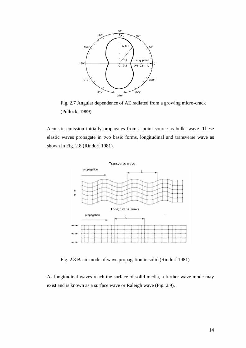
Fig. 2.7 Angular dependence of AE radiated from a growing micro-crack
(Pollock, 1989)
Acoustic emission initially propagates from a point source as bulks wave. These
elastic waves propagate in two basic forms, longitudinal and transverse wave as
shown in Fig. 2.8 (Rindorf 1981).
Fig. 2.8 Basic mode of wave propagation in solid (Rindorf 1981)
As longitudinal waves reach the surface of solid media, a further wave mode may
exist and is known as a surface wave or Raleigh wave (Fig. 2.9).
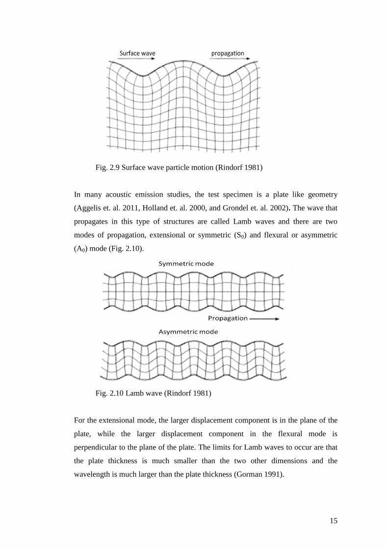
15
Fig. 2.9 Surface wave particle motion (Rindorf 1981)
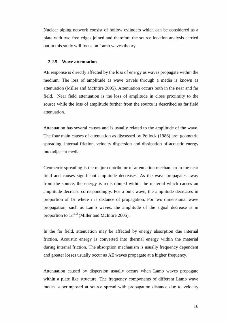
In many acoustic emission studies, the test specimen is a plate like geometry
(Aggelis et. al. 2011, Holland et. al. 2000, and Grondel et. al. 2002). The wave that
propagates in this type of structures are called Lamb waves and there are two
modes of propagation, extensional or symmetric (S0) and flexural or asymmetric
(A0) mode (Fig. 2.10).
Fig. 2.10 Lamb wave (Rindorf 1981)
For the extensional mode, the larger displacement component is in the plane of the
plate, while the larger displacement component in the flexural mode is
perpendicular to the plane of the plate. The limits for Lamb waves to occur are that
the plate thickness is much smaller than the two other dimensions and the
wavelength is much larger than the plate thickness (Gorman 1991).
16
Nuclear piping network consist of hollow cylinders which can be considered as a
plate with two free edges joined and therefore the source location analysis carried
out in this study will focus on Lamb waves theory.
2.2.5 Wave attenuation
AE response is directly affected by the loss of energy as waves propagate within the
medium. The loss of amplitude as wave travels through a media is known as
attenuation (Miller and McIntire 2005). Attenuation occurs both in the near and far
field. Near field attenuation is the loss of amplitude in close proximity to the
source while the loss of amplitude further from the source is described as far field
attenuation.
Attenuation has several causes and is usually related to the amplitude of the wave.
The four main causes of attenuation as discussed by Pollock (1986) are; geometric
spreading, internal friction, velocity dispersion and dissipation of acoustic energy
into adjacent media.
Geometric spreading is the major contributor of attenuation mechanism in the near
field and causes significant amplitude decreases. As the wave propagates away
from the source, the energy is redistributed within the material which causes an
amplitude decrease correspondingly. For a bulk wave, the amplitude decreases in
proportion of 1/r where r is distance of propagation. For two dimensional wave
propagation, such as Lamb waves, the amplitude of the signal decrease is in
proportion to 1/r1/2
(Miller and McIntire 2005).
In the far field, attenuation may be affected by energy absorption due internal
friction. Acoustic energy is converted into thermal energy within the material
during internal friction. The absorption mechanism is usually frequency dependent
and greater losses usually occur as AE waves propagate at a higher frequency.
Attenuation caused by dispersion usually occurs when Lamb waves propagate
within a plate like structure. The frequency components of different Lamb wave
modes superimposed at source spread with propagation distance due to velocity
17
variations. This type of attenuation can be very large for highly attenuated
dispersive mode such as guided waves in ultrasonic testing.
The fourth attenuation mechanism is dissipation of acoustic energy into adjacent
media. Scattering of AE signals due to internal scattering from in-homogeneities
such as grains in metals can cause this type of attenuation. Other sources of this
kind of attenuation are surface coating and fluids contained in vessel or piping
system.
To avoid the AE signal escaping detection due to attenuation, several transducers
should be placed close together to ensure that an AE event emanating from any
region on the structure can be detected. The minimum spacing between two sensors
can be identified empirically through simulated AE testing or through experience
with similar structures.
Attenuation can be measured by placing several sensors at different distances from
an AE source. Attenuation can be calculated as:
= 20/x log A1/A2 (2.1)
Where:
is attenuation coefficient (decibels over distances); x is distance between detection
points; A1 is amplitude of signal at point 1; and A2 is amplitude of signal at point 2.
Attenuation coefficient is a function of the frequency content of the AE wave and
the medium of wave propagation.
2.3 Modal analysis
The wave propagation in plate like structure is complicated because of the
interaction of the wave with its two free surfaces. Complicated resonant conditions
occur as the frequency changes and propagation can occurs in a series of symmetric
and asymmetric modes. The way in which acoustic wave propagates in plate like
structures is governed by Lamb wave theory, also known as plate wave theory
(Gorman 1991).
18
Lamb wave propagation and velocity are very strongly dependent upon both
frequency content and plate thickness. The dependency of velocity upon frequency
is known as dispersion and any particular frequency can propagate a number of
different velocities (Pollock 1986, Holford 2000). Multiple symmetric and
asymmetric Lamb wave modes could exist together at given signal frequency. The
number of coexisting wave-modes goes up as the frequency-thickness product is
increased (Harker, 1988).
Conventional AE analysis techniques have mainly utilised simple signal parameters
like amplitude, duration, counts and energy and the rate at which AE signals
occurred. In an alternative to this conventional technique, the dispersive nature of
Lamb wave can be exploited and is known as modal acoustic emission (Holford
2000).
2.3.1 Modal Acoustic Emission (MAE)
MAE uses wideband and high fidelity instrumentation to detect and capture the
transient wave associated with defect growth (Chang 2006). The MAE technique
involves the determination of the arrival time of S0 (extensional) and A0 (flexural)
wave components and computing the distance of the source to sensor by measuring
their temporal separation of the source waveform (Holford 2000, Pullin 2007).
A few researchers have observed flexural and extensional mode propagation in
plate like structures. Gorman (1991) studied signals in aluminium and composite
plates using a range of sensor types. He demonstrated the occurrence of the
fundamental flexural and extensional components and observed that the two modes
have significantly different frequency contents and dispersion characteristics.
Using signals obtained from the testing of carbon fibre reinforced polymer (CFRP),
Surgeon and Wevers (1999) determined the difference in arrival times for
symmetric and asymmetric modes. The difference in arrival times of symmetric and
asymmetric modes is calculated based on simple plate wave theory and was
compared with measured values of separation and the results were in good
agreement.
19
Based on modal characteristic of the wave mode propagation in plate like structures,
the velocity and the different arrival time of these modes could be used for accurate
source location. Since the detection of the arrival time of different modes is not
determined by a preset threshold of data acquisition, it is expected that SSMAL will
produce more accurate source location (Surgeon, 1999) compared with the
traditional based source location method. Ziola and Gorman (1991) suggested that
accurate linear location can only be performed if the modal nature of AE signals is
taken into account.
Maji and Sapathi (1995), Dunegan (1997) and Holford (1999) have demonstrated
that the location of pencil lead break sources using single sensor source location
can be carried out by band pass filtering. Filtering of the original signal to high
frequency content and low frequency content was used to establish the arrival of S0
and A0 modes to estimate source to sensor distance.
Pullin (2005) used the two fundamental components of Lamb waves for estimating
the artificial and fatigue crack source to sensors distance in aerospace grade steel.
He showed that, in a controlled laboratory study of fatigue crack growth, it is
possible to calculate the distance of a fatigue crack source from a single sensor with
reasonable accuracy.
Nevertheless, this method also suffers from some drawbacks. The arrival time of A0
and S0 modes is often difficult to determine due to the superposition of these
fundamental modes with reflections from specimen boundaries, superposition with
other wave modes and also from noise signals. Furthermore, the uses of incorrect
modes will contribute to a larger error in SSMAL measurement when compared
with the commercial TOA method.
2.3.2 Dispersion Curve
Dispersion curves are a very useful tool in MAE. Dispersion curves are generated
by plotting either phase or group velocity values against their frequency-thickness
20
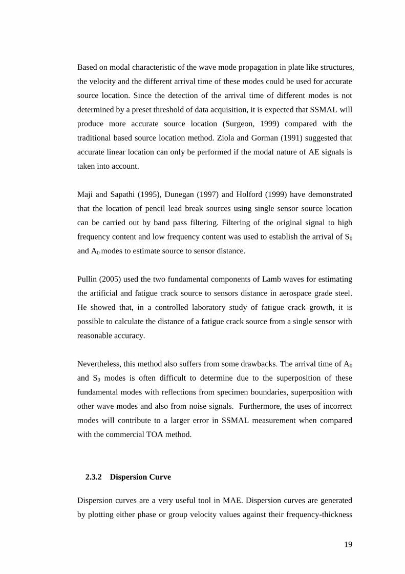
products. The curves are displayed as a function of velocity on the vertical axis and
frequency (or thickness-frequency) on the horizontal axis from the test item setup
as shown in Fig. 2.11.
Fig. 2. 11 Typical dispersion curves for 10 mm steel plate (generated using PAC
Sharewavelet software)
The dispersion curves illustrate how, for a fixed plate thickness, different frequency
components of lamb waves travel at different velocities. If the wave is detected by a
suitable transducer, separation of the difference frequency components can be
observed and respective arrival times can be measured. The dispersion curve graph
can be modified in a variety of ways to help the user visualise the wave propagation
characteristics.
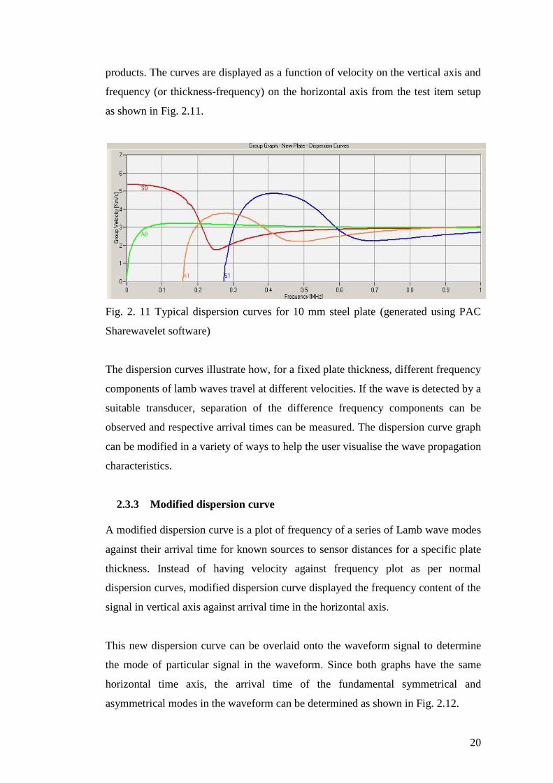
2.3.3 Modified dispersion curve
A modified dispersion curve is a plot of frequency of a series of Lamb wave modes
against their arrival time for known sources to sensor distances for a specific plate
thickness. Instead of having velocity against frequency plot as per normal
dispersion curves, modified dispersion curve displayed the frequency content of the
signal in vertical axis against arrival time in the horizontal axis.
This new dispersion curve can be overlaid onto the waveform signal to determine
the mode of particular signal in the waveform. Since both graphs have the same
horizontal time axis, the arrival time of the fundamental symmetrical and
asymmetrical modes in the waveform can be determined as shown in Fig. 2.12.
21
Fig. 2.12 Illustration on how a modified dispersion curve overlaid on waveform
can be used to determine the arrival of Lamb wave modes
2.4 AE source location
2.4.1 Introduction
Locating the source of significant AE is often the main goal of an inspection. AE
systems are capable of using multiple sensors during testing, allowing them to
record a hit from a single AE event. As hits are recorded by each sensor/channel,
the source can be located by knowing the velocity of the wave in the material and
the difference in arrival times among the sensors, as measured by hardware
circuitry or computer software. By properly spacing the sensors in this manner, it is
possible to inspect an entire structure with relatively few sensors (Miller and
McIntire 2005, Pollock 1989).
Most source location techniques assume that AE waves travel at a constant velocity
in a material. However, various effects may alter the expected velocity of the AE
waves such as reflections and multiple wave modes which can affect the accuracy
of this technique. Therefore, the geometric effects of the structure being tested and
the operating frequency of the AE system must be considered when determining
whether a particular source location technique is feasible for a given test structure
(Baxter 2007).
22
Good knowledge of source location is the basic requirement for further
characterisation of a damage mechanism. Calculation of the AE source location is
mostly based on arrival time differences of the signals recorded by different
transducers. Errors in arrival time determination and elastic wave velocity
measurement can crucially affect the inaccuracy of AE source location (Miller and
McIntire, 2005).
2.4.2 Time of Arrival (TOA) source location
The AE event causes a micro-seismic wave that travels within the material and is
detected by the transducers and the time of arrival is then determined. Usually, the
AE events are located based on the time of arrival at a number of transducers, using
the known distances between the transducers and the P-wave (bulk longitudinal
wave) propagation velocity. This method is known as time of arrival (TOA)
approach (Miller and McIntire 2005, Rindorf 1981).
Time of Arrival (TOA) source location is the most widely used method for AE
source location. This method is based on the measurement of time difference
between the arrivals of individual AE events at different sensors in an array and is
the basis of most commercial AE software.
The sensors are arranged either in linear, triangular or rectangular arrays. In order
for point location to be justified, signals must be detected by a minimum number of
two sensors for linear, three for planar and four for volumetric location.
Linear location methods can be explained by considering an array of three sensors
along a beam. An AE event occurring at any point in this beam will emit stress
waves which propagate in both directions. The simplest method of locating this
event is using zonal location.
This method examines the order in which the AE signal reaches the sensors in its
array. By noting which sensor is ‘hit’ first, the zonal location can be determined. In
Fig. 2.13 a), sensor 2 is hit first and therefore the source must have come from an
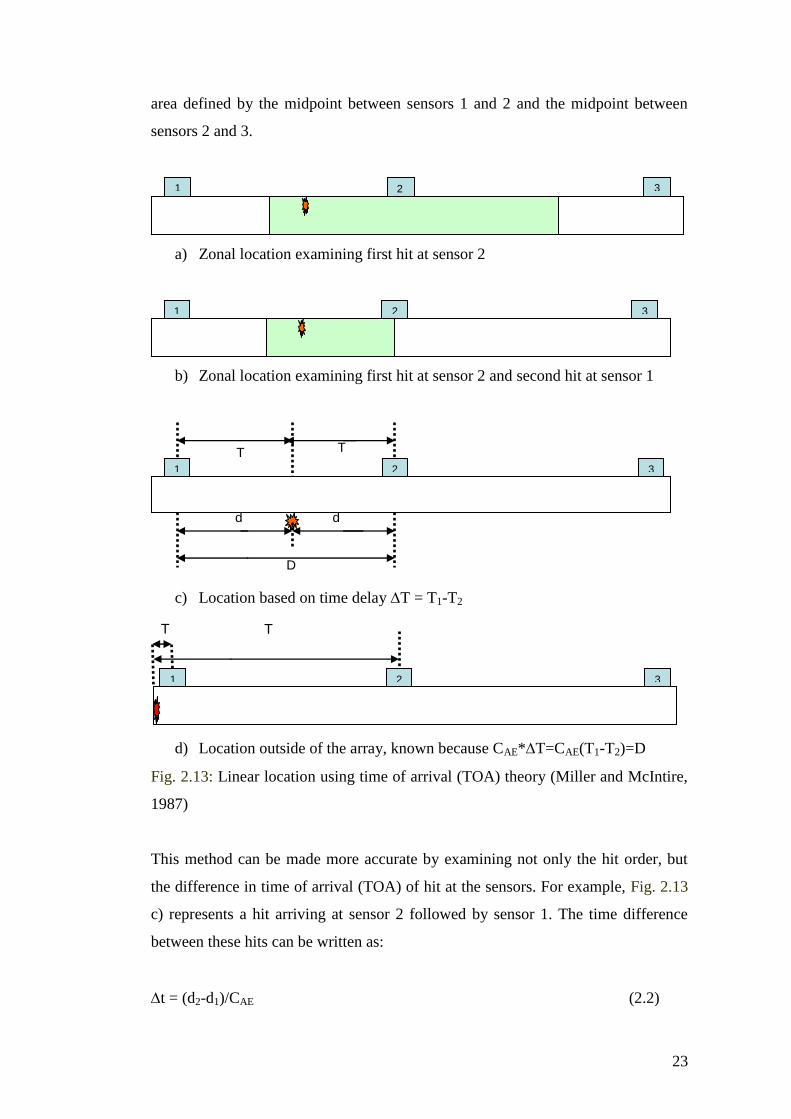
23
area defined by the midpoint between sensors 1 and 2 and the midpoint between
sensors 2 and 3.
a) Zonal location examining first hit at sensor 2
b) Zonal location examining first hit at sensor 2 and second hit at sensor 1
c) Location based on time delay T = T1-T2
d) Location outside of the array, known because CAE*T=CAE(T1-T2)=D
Fig. 2.13: Linear location using time of arrival (TOA) theory (Miller and McIntire,
1987)
This method can be made more accurate by examining not only the hit order, but
the difference in time of arrival (TOA) of hit at the sensors. For example, Fig. 2.13
c) represents a hit arriving at sensor 2 followed by sensor 1. The time difference
between these hits can be written as:
t = (d2-d1)/CAE (2.2)
1 2 3
T
2
T
1
1 2 3
T
2
T
1
D
d
2
d
1
1 2 3
1 3
2
24
where: CAE = calculated wave velocity
t = time difference between sensors
d1 = distance from source to first hit sensor
d2 = distance from source to second hit sensor
This is however, commonly expressed in terms of d1
d1= (D-CAE. t) /2 (2.3)
where D= total distance between sensors
If the source originates from outside the array, Fig. 2.13 d), then the time difference
between the two signals will become equal to the time taken for the wave to travel
between the two sensors. The source will be located at the sensor at the edge of the
array; in this case of the example, at sensor 1.
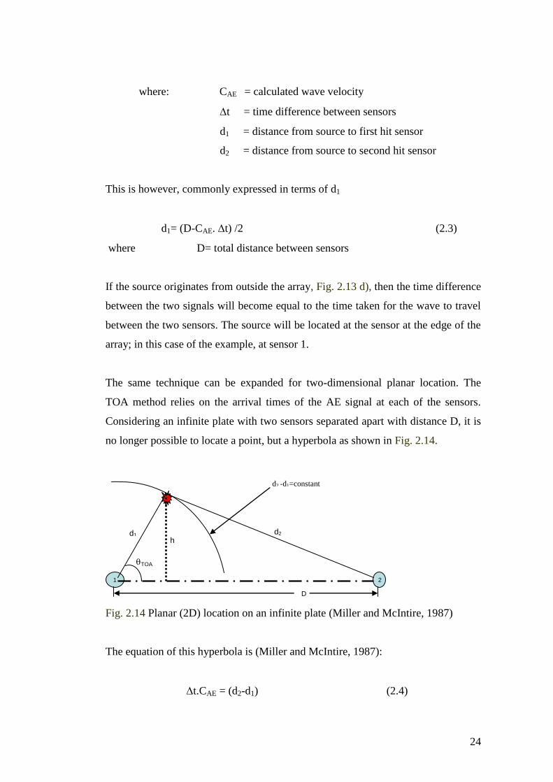
The same technique can be expanded for two-dimensional planar location. The
TOA method relies on the arrival times of the AE signal at each of the sensors.
Considering an infinite plate with two sensors separated apart with distance D, it is
no longer possible to locate a point, but a hyperbola as shown in Fig. 2.14.
Fig. 2.14 Planar (2D) location on an infinite plate (Miller and McIntire, 1987)
The equation of this hyperbola is (Miller and McIntire, 1987):
t.CAE = (d2-d1) (2.4)
1 2
d1 d2
D
d2 -d1=constant
TOA
h
25
and h = d1 Sin TOA (2.5)
h2 = d2
2 – (D- d1 TOA)
2 (2.6)
then d12 sin
2TOA = d2
2 – (D- d1cosTOA)
2 (2.7)
d12 = d2
2 – D
2 - 2Dd1 TOA
substituting d2 = d1 + t.CAE from the (2.3) gives:
d1 = ½ ((D2
- t2CAE
2) / (2tCAE + DcosTOA)) (2.8)
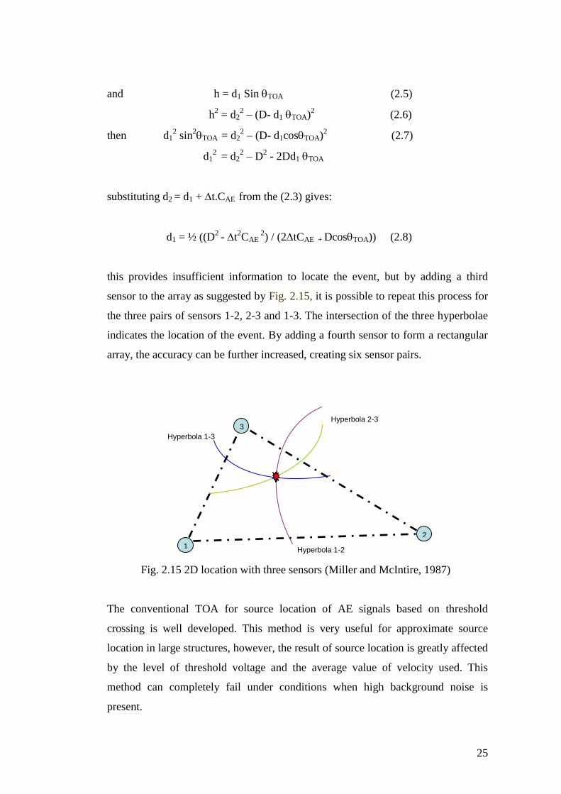
this provides insufficient information to locate the event, but by adding a third
sensor to the array as suggested by Fig. 2.15, it is possible to repeat this process for
the three pairs of sensors 1-2, 2-3 and 1-3. The intersection of the three hyperbolae
indicates the location of the event. By adding a fourth sensor to form a rectangular
array, the accuracy can be further increased, creating six sensor pairs.
Fig. 2.15 2D location with three sensors (Miller and McIntire, 1987)
The conventional TOA for source location of AE signals based on threshold
crossing is well developed. This method is very useful for approximate source
location in large structures, however, the result of source location is greatly affected
by the level of threshold voltage and the average value of velocity used. This
method can completely fail under conditions when high background noise is
present.
1
2
3 Hyperbola 2-3
Hyperbola 1-3
Hyperbola 1-2
26
The sources of error are fully investigated by Rindorf (1981) and detailed
explanation can be found in Miller and McIntire (2005). However, according to
Holford (2000), the main sources of error associated with the TOA method are:
Premature triggering of detection threshold by a low amplitude symmetric
component – timing is usually based on the arrival of the asymmetry
(flexural) component.
Dispersion of the asymmetric mode component – wave dispersion within
the structure will cause alterations in the waveform. This may cause the
detection threshold triggered by a different phase of the signal.
Different wave-paths due to inhomogeneitis in structure.
Other sources of error include inaccurate sensor location, incorrect group wave
velocity and human error.
2.4.3 DeltaT location
The Delta location method as proposed by Baxter (2007) utilises an artificial source
to acquire the time of arrival data at each sensor within an array. This method also
utilises the time arrival of AE signal at the sensor, as with the TOA methods;
however, a location is derived from a user defined map system rather than using an
average velocity.
The arrival time difference (T) is analysed at pairs of sensors within an array. A
map is constructed displaying contour lines of equal T sources for each sensor
pair. Any previous, current or future AE data received from within the mapped area
can be overlaid on T maps to identify the source location without considering the
wave path and wave speeds (Baxter 2007).
The T location method involves five major steps as outlined below;
o Determine area of interest – The area where the crack is expected to initiate
and growth is first determined.
o Grid construction – a grid is constructed in the area of interest on an
engineering component in which future AE events will be located. The
resolution of the grid should be as higher as possible for higher source
27
location accuracy. Sources are located with reference to the grid applied to
structure rather than sensor location.
o Obtain TOA of training data – Pencil lead break (H-N source) is conducted
at each node on the grid to obtain the time arrival data at each sensor. It is
essential to have enough AE sources at each node to provide reliable result
and to eliminate erroneous data. At least five sources at each node are
required to provide a reliable result.
o T map calculation – For each H-N source, the TOA time difference (T)
for each sensor pair are calculated. An array of three sensors has three
sensor pairs 1-2, 1-3 and 2-3 while array of four sensors has six sensor pairs
(1-2, 1-3, 1-4, 2-3, 2-4 and 3-4). The average T for each sensor pair at each
node is stored in a map. The maps can be displayed as contour plots of equal
T.
o AE source location – To locate an actual event from an AE source, T for
each sensor pair is calculated. A line or contour on each map corresponding
to the calculated T can be identified. Source locations are determined by
overlying the results from each sensor pairs and identifying their
convergence point. For source location using an array of four sensors, six
lines from six sensor pairs will be used and these six lines are expected to
intersect at one point to give the location of the source.
The T location method cannot be used for complete coverage of structure but it is
suggested to be used as a tool to improve source location around critical or
complicated areas. This method overcomes the assumption that the wave
propagates with constant velocity in the straight path which is untrue for structures
with multiple thickness changes. A further advantage of the DeltaT source location
method is that new areas of interest can be added during or post test and therefore
active areas identified by TOA can also be more accurately assessed (Baxter, 2007).
According to Baxter (2007), this method has an associated error equivalent to one
grid square.
28
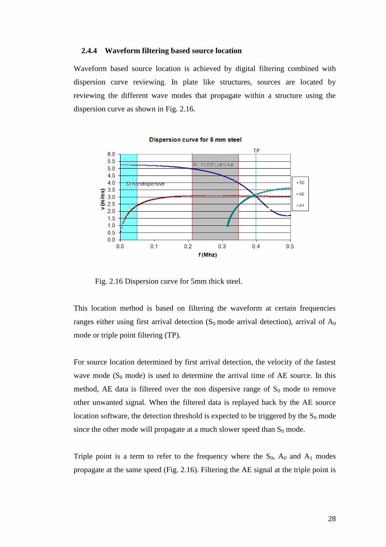
2.4.4 Waveform filtering based source location
Waveform based source location is achieved by digital filtering combined with
dispersion curve reviewing. In plate like structures, sources are located by
reviewing the different wave modes that propagate within a structure using the
dispersion curve as shown in Fig. 2.16.
Fig. 2.16 Dispersion curve for 5mm thick steel.
This location method is based on filtering the waveform at certain frequencies
ranges either using first arrival detection (S0 mode arrival detection), arrival of A0
mode or triple point filtering (TP).
For source location determined by first arrival detection, the velocity of the fastest
wave mode (S0 mode) is used to determine the arrival time of AE source. In this
method, AE data is filtered over the non dispersive range of S0 mode to remove
other unwanted signal. When the filtered data is replayed back by the AE source
location software, the detection threshold is expected to be triggered by the S0 mode
since the other mode will propagate at a much slower speed than S0 mode.
Triple point is a term to refer to the frequency where the S0, A0 and A1 modes
propagate at the same speed (Fig. 2.16). Filtering the AE signal at the triple point is
29
expected to produce more accurate source location result since the detection
threshold is expected to be triggered simultaneously by the S0, A0 and A1 mode.
2.4.5 Single Sensor Modal Analysis Location (SSMAL)
Conventional AE locations technique have mainly utilised the arrival time of first
threshold crossing. An alternative to this conventional technique exploits the
dispersive nature of Lamb waves and is known as modal acoustic emission (MAE)
(Gorman 1991, Posser 1992). For a fixed plate thickness, different frequency
components of Lamb waves travel at different velocity.
Single sensor modal analysis location (SSMAL) works on the MAE theory.
SSMAL utilised the time delay of the S0 and A0 modes of waveform signals (time
domain signals) and the distance of the source from sensor is determined by the
velocity of two modes and their time delay (Holford, 1999 and Pullin 2005). If the
two basic components of lamb waves, S0 and A0, travel at different velocities CS0
and CA0, and the time lapse (Δt) between their arrival is measured, then the source
to sensor distance (D) is given by;
D = Δt (CS0CA0/ CS0-CA0) (Pullin et. al, 2007). (2.9)
SSMAL method also suffers from some drawbacks. The arrival of A0 is often
difficult to determine due to the superposition of this fundamental mode with
reflection signals from specimen boundaries, superposition with other wave modes
and also from noise. This can cause incorrect mode arrival time determination
which leads to temporal separation measurement error.
Furthermore, the use of the incorrect mode arrival time of A0 mode will contribute
to a larger error in SSMAL measurement when compared with the commercial
TOA method. To overcome this drawback, a modified dispersion curve as
discussed in section 2.3.4 can be used to verify the temporal separation
measurement however this curve can only be produced if the source to sensor
distance is known.
30
SSMAL location method promises an accurate source location result if the temporal
separation error due to the superposition of A0 mode with other wave components
can be resolved. Temporal separation measurement error in SSMAL can be
improved by deploying time-frequency analysis such as wavelet transform which
can discriminate the content of AE signal.
2.5 Wavelet transform
2.5.1 Introduction AE signal analysis
The AE signal processing method is divided into time domain analysis and
frequency domain analysis. Temporal separation determination of fundamental
Lamb wave modes for single sensor modal analysis location (Pullin 2007) is the
typical time domain analysis. Frequency spectrum analysis describes the frequency-
domain characteristics of an AE signal. The Fourier Transforms (FT) spectrum
analysis and spectrum estimations are typical spectrum analysis methods
(Takemoto 2000).
The FT is only able to retrieve the frequency content of the signal but at the same
time it loses any temporal information. This is overcome by a Short Time Fourier
Transform (STFT) which calculates the FT of a part of a signal as a window and
shifts the window over the entire signal. However, the STFT gives the content of a
signal with a constant time and frequency resolution due to the fixed window length
(Takemoto 2000). For analysing AE Lamb wave signals propagating in plate like
components, this is not the desired resolution. The broadband and dispersive nature
of Lamb waves need a multi resolution analysis and it is possible by using a
wavelet analysis (Takemoto 2000).
Wavelet transform (WT) theory is a signal processing method which overcomes the
limitation of Fourier analysis by performing time- frequency analysis at the same
time. It also solves the conflict of time and frequency resolution in STFT analysis
(Takemoto 2000). Detailed mathematical derivation on STFT and WT and their
construction methods is well explained by Daubechies (1999).
31
Wavelet analysis has attracted attention in AE signal processing for its ability to
analyse rapidly changing transient signal (Jeong 2000). WT analysis is suitable for
processing transient AE signals because it not only describes the signal spectrum
corresponding to a local time, but also describing the time-domain information
within that spectrum (Serrano 1996).
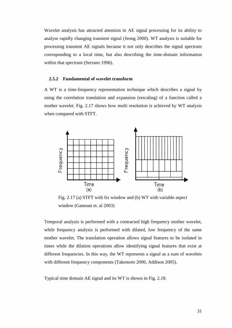
2.5.2 Fundamental of wavelet transform
A WT is a time-frequency representation technique which describes a signal by
using the correlation translation and expansion (rescaling) of a function called a
mother wavelet. Fig. 2.17 shows how multi resolution is achieved by WT analysis
when compared with STFT.
Fig. 2.17 (a) STFT with fix window and (b) WT with variable aspect
window (Ganesan et. al 2003)
Temporal analysis is performed with a contracted high frequency mother wavelet,
while frequency analysis is performed with dilated, low frequency of the same
mother wavelet. The translation operation allows signal features to be isolated in
times while the dilation operations allow identifying signal features that exist at
different frequencies. In this way, the WT represents a signal as a sum of wavelets
with different frequency components (Takemoto 2000, Addison 2005).
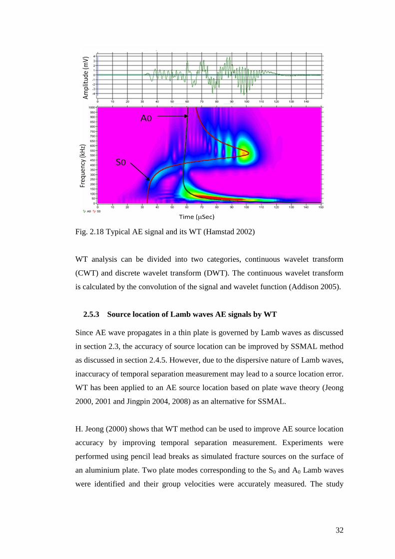
Typical time domain AE signal and its WT is shown in Fig. 2.18.
32
Fig. 2.18 Typical AE signal and its WT (Hamstad 2002)
WT analysis can be divided into two categories, continuous wavelet transform
(CWT) and discrete wavelet transform (DWT). The continuous wavelet transform
is calculated by the convolution of the signal and wavelet function (Addison 2005).
2.5.3 Source location of Lamb waves AE signals by WT
Since AE wave propagates in a thin plate is governed by Lamb waves as discussed
in section 2.3, the accuracy of source location can be improved by SSMAL method
as discussed in section 2.4.5. However, due to the dispersive nature of Lamb waves,
inaccuracy of temporal separation measurement may lead to a source location error.
WT has been applied to an AE source location based on plate wave theory (Jeong
2000, 2001 and Jingpin 2004, 2008) as an alternative for SSMAL.
H. Jeong (2000) shows that WT method can be used to improve AE source location
accuracy by improving temporal separation measurement. Experiments were
performed using pencil lead breaks as simulated fracture sources on the surface of
an aluminium plate. Two plate modes corresponding to the S0 and A0 Lamb waves
were identified and their group velocities were accurately measured. The study
33
showed that the source location measured by this approach mostly agreed with the
actual locations.
Gabor wavelet has been used in the analysis of AE signals due to its good
resolution in both time and frequency domain. The frequency component in the
output signal has been extracted from the output of the envelope of a WT (Jeong
2001, Jingpin 2008).
H. Jeong (2000) applied the WT using Gabor wavelet to the analysis of flexural
transient wave propagation in anisotropic composite laminates. He found that
dispersion of the flexural mode obtained by WT analysis shows a good agreement
with experimental results. Based on his analysis, the peak of WT analysis amplitude
is related to the arrival time of the group velocity and the arrival time of each
frequency has been successfully determined by WT analysis.
In principal, both Jeong and Jinpin used peak amplitude of AE signals to determine
the arrival of fundamental mode and temporal separation. Most of the conventional
TOA based AE system use first threshold crossing to determine the arrival AE
signal rather than peak amplitude. It is expected that the minimum value of wavelet
coefficient magnitude for each mode component could be more accurate for
determining mode arrival times.
Aljets (2010) used WT to pick the arrival time of S0 and A0 modes and located the
AE source in a large plate like structures using a local triangular sensor array. He
found that, there is a possibility to wrongly pick the arrival time of the mode of
interest which leads to significant location error. This error may make worse by
noisy testing environment.
2.5.4 Signal denoising of AE using Discrete Wavelet Transform (DWT)
AE signals are broadband and contain environmental and electrical noises. This
noise signal should be eliminated before further signal analysis is carried out and
this can be done by performing DWT analysis.
34
The denoising of signals using the wavelet transform is done by representing the
signal by a small number of coefficients. The waveform is decomposed into a series
of wavelet coefficients. Each coefficient has different amplitudes at the various
locations and durations. The wavelet coefficient is related to position (or time) and
frequency of waveform (Zhao 2000).
Many of the wavelet coefficients generated by the WT are at a coefficient value
near zero. They add very little to the composition of the waveform itself and most
of them are produced by noise in the waveform. By applying a threshold process,
these noise signal coefficients can be removed without affecting the integrity of the
original signal. DWT is a very powerful tool for denoising and filtering certain
components of AE signals when combined with the inverse DWT (Takemoto 2000).
Signal denoising using wavelet analysis has several advantages compared with
conventional filtering methods. It can reduce the noise of a signal and at the same
time keep the original features of the signal. Detailed signal denoising using WT
can be found in Alfouri (2008) and common steps to reduce high frequency noise
using wavelet denoising can be summarised as follow:
i) Discrete wavelet transform are calculated based on the best mother
wavelet
ii) Wavelet coefficient threshold are applied onto the waveform to
eliminate high frequency noise
iii) Waveform are reconstructed by inverse transform and normalising
2.5.5 Signal characterisation using WT analysis
WT method is not just useful for source location and signal denoising but also can
be used for source identification or defect/damage characterisation. Some work has
been carried out to utilise WT analysis to characterise the AE signal. Zhihao (2009)
combined WT with the energy analysis to study the AE signal from the rubbing
fault of a rotary machine. AE feature of the rubbing fault was successfully
extracted by using this method.
35
Gang Qi (2000) used wavelet analysis to study the fracture behaviour on glass fibre
reinforced plastic. He found that wavelet based methods could approximate residual
strength better than classical AE technique.
Hamstad (2002) was used A0/S0 ratio based on WT analysis to distinguish different
sources types all centred at the same depth below the plate surface and with the
same propagation system. He found that the values of this ratio overlapped for
different source types at different depths and concluded that it is not possible to
uniquely identify the source type with a small set of WT -based data.
2.6 Thermal fatigue
2.6.1 Introduction to fatigue
Fatigue is the progressive, localised, and permanent structural change that occurs in
a material subjected to repeated or fluctuating strains at nominal stresses that have
maximum values less than (and often much less than) the static yield stress of the
material (Fine and Chung 1996 ).
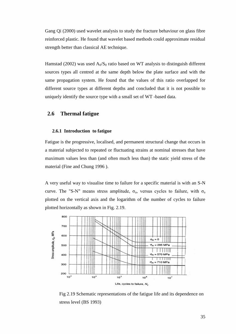
A very useful way to visualise time to failure for a specific material is with an S-N
curve. The "S-N" means stress amplitude, σa, versus cycles to failure, with σa
plotted on the vertical axis and the logarithm of the number of cycles to failure
plotted horizontally as shown in Fig. 2.19.
Fig 2.19 Schematic representations of the fatigue life and its dependence on
stress level (BS 1993)
36
Fatigue may produce cracks and cause fractures after a sufficient number of cycles.
According to BS (1993), failure of a material due to fatigue may be viewed on
microscopic level in three steps:
i. Crack Initiation: The initial crack occurs in this stage. The crack may be caused
by surface scratches caused by slip bands or dislocations intersecting the
surface as a result of previous cyclic loading or work hardening.
ii. Crack Propagation: The crack continues to grow during this stage as a result of
continuously applied stress range.
iii. Failure: Failure occurs when the material that has not been affected by the crack
cannot withstand the applied stress range. This stage often happens very quickly.
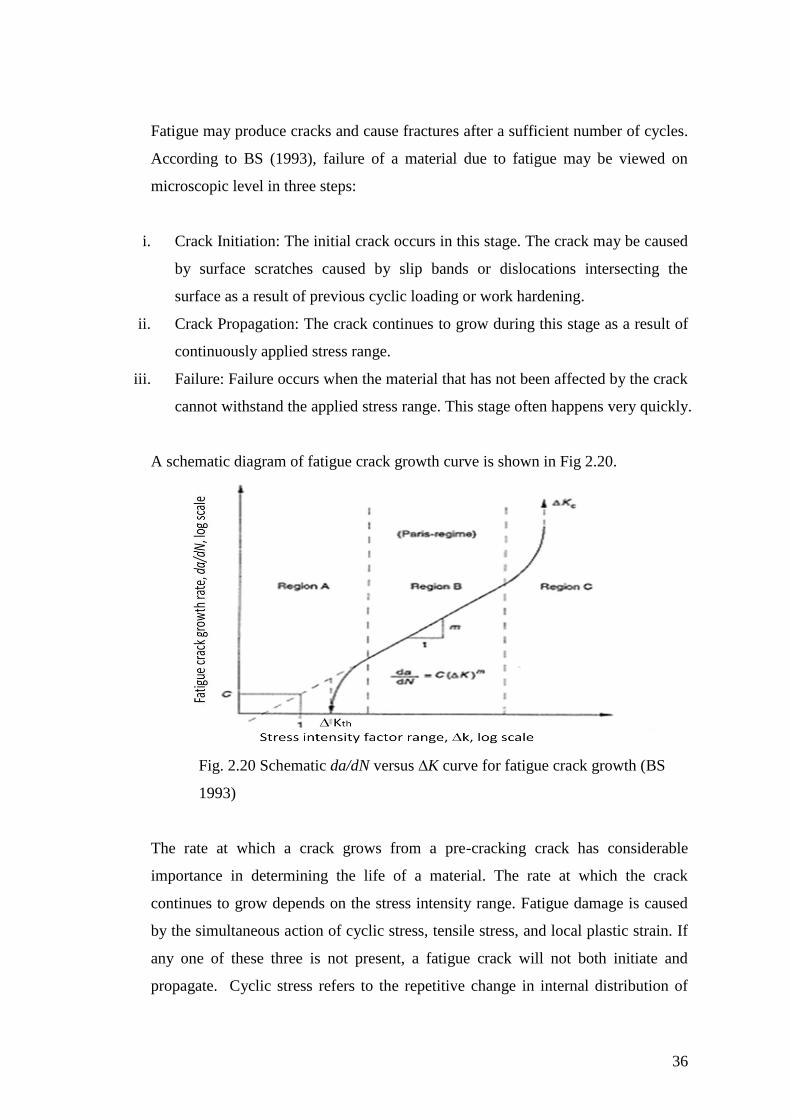
A schematic diagram of fatigue crack growth curve is shown in Fig 2.20.
Fig. 2.20 Schematic da/dN versus ∆K curve for fatigue crack growth (BS
1993)
The rate at which a crack grows from a pre-cracking crack has considerable
importance in determining the life of a material. The rate at which the crack
continues to grow depends on the stress intensity range. Fatigue damage is caused
by the simultaneous action of cyclic stress, tensile stress, and local plastic strain. If
any one of these three is not present, a fatigue crack will not both initiate and
propagate. Cyclic stress refers to the repetitive change in internal distribution of
37
force and it can be in form of load, pressure or temperature. Damage caused by
thermal cyclic loading is called thermal fatigue.
2.6.2 Thermal fatigue in nuclear piping
Thermal fatigue cracks have been reported to occur in primary loop recirculation
pipes and various other components of nuclear power plants (Hayashi, 1998). The
main source of fatigue cracks in the nuclear piping system is the thermal stresses
associated with plant heat-up and cool down which were not included in the
original fatigue design analyses. For example, thermal fatigue cracks were initiated
at a branch pipe connection between a feed water system and shut down cooling
system (Hayashi, 1998).
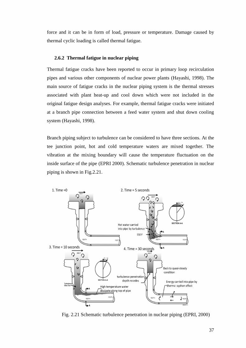
Branch piping subject to turbulence can be considered to have three sections. At the
tee junction point, hot and cold temperature waters are mixed together. The
vibration at the mixing boundary will cause the temperature fluctuation on the
inside surface of the pipe (EPRI 2000). Schematic turbulence penetration in nuclear
piping is shown in Fig.2.21.
Fig. 2.21 Schematic turbulence penetration in nuclear piping (EPRI, 2000)
38
In the section closest to the run pipe, the entire pipe’s cross section is at a hot
temperature. In the second section, the run pipe temperature permeates into the
branch pipe, but to a lesser extent, such that it stratifies at the top of the pipe.
Combined with this are flow turbulence effects, which cause local thermal cycling
at points in the pipe cross-section. In the third section of turbulence penetration,
further away from the run pipe, only the effects of run pipe temperature permeating
into the pipe due to natural convection effects are present. There is no flow
turbulence across the cross section. However, cycling can still occur in this region,
as the length of turbulence penetration may produce temperature variations over
time in both the axial and radial directions.
Thermal stratification may also cause leaks in normally stagnant lines connected to
the reactor coolant loop in safety injection systems, reactor coolant drain lines, a
residual heat removal suction line, and an excess letdown line. In addition,
stratification has caused cracking of steam generator feed water nozzles and high
piping displacements in pressuriser surge lines (Bieniussa 1999).
Thermal fatigue can lead to crack formation, small leaks in piping, medium leaks in
piping (when crack opening is more than 1 mm) or a total break of piping system
(NEA/CSNI/R, 2005). The leak before break (LLB) concept is widely used in the
nuclear industry to describe the idea that in the piping carrying the coolant of power
reactor, a leak will develop before a catastrophic failure will occur (IAEA 1993).
The LLB concept is based on a fracture mechanic approach that a crack would
grow through the wall of piping system, resulting in a leak, and that this postulated
small ‘through wall’ defect in plant piping would be detected by a leakage
monitoring system before the flaw could grow to critical size. Leakage exceeding a
specified limit requires the plant to be shut down (IAEA 1993).
For the application of the LLB concept to take place in the nuclear power plant,
leak detection methods must be added to the plant. However, no single currently
available leak detection method can provide optimal detection sensitivity, location
ability and measurement accuracy. Although quantitative leakage determination is
39
possible by using condensate flow monitors (Kupperman 1985), sump monitors and
primary coolant inventory balance, these methods are not adequate for locating and
measuring leak size and are not sensitive enough to meet LLB requirements (IAEA
1993)
Currently, piping structures in nuclear power plants are inspected using
conventional non-destructive methods like ultrasonic testing which are carried out
during power plant shut down, which are usually held every 10 years (IAEA, 2003).
If cracks due to thermal fatigue occur within this period, it will be left unattended
unless a proper continuous leak monitoring system is installed to monitor such
failure in piping systems in nuclear power plant. This type of critical failure not just
causes leaks of radioactive material into the environment but also may contribute to
the catastrophic failure of the nuclear power plant.
A suitable technology to improve leak detection capability at specified sites in the
nuclear power piping is the use of AE monitoring. AE offers the opportunity to
monitor the thermal fatigue damage continuously and cracks can be identified at
early initiation stage without intrusion on the plant operation schedule. However,
current AE techniques still have difficulties with sources discrimination and flaw
size measurement.
With current development in WT analysis, it may be possible that the MAE
technique can detect, identify and measure the size of thermal fatigue cracks in
piping systems in a more accurate manner.
2.6.3 Fatigue and AE
AE from crack growth is of interest for practical non-destructive testing
applications. The formation of the stress concentrations in their vicinity, cracks and
other defects will emit stress waves when load is increased, while an unflawed part
in material will remain silent. It is useful to distinguish between AE signals from
the plastic zone at the crack tip and AE signals from the movement of the crack
itself. If the size of the plastic zone is very big, the signal released from this
mechanism will not represent the actual location of the crack tip. Growth of the
40
plastic zone typically produces many emissions of low amplitude (Khan 1982,
Talebzadeh 2001).
AE from the crack front movement depends on the nature of the crack growth
process. Microscopically, rapid mechanisms such as brittle inter-granular fracture
and trans-granular cleavage are detectable when the crack front is advancing one
grain at sub-critical stress levels. Slow, continuous crack growth mechanism such
as micro-void coalescence and active path corrosion are not detectable in
themselves but they may be detectable through associated plastic zone growth
(Miller, 1987).
AE monitoring, together with fracture mechanics methods, have been used to study
cleavage crack growth in laboratory specimens of several alloy steels. Experimental
results indicate that, during the onset of rapid unstable crack growth, spontaneous
acoustic events are emitted. The fractographic studies on the fractured surface have
demonstrated that a large number of energetic signals result from local brittle
fracture at the crack tip. It was found that the stress intensity factor corresponding
to the first trans-granular or inter-granular cleavage crack extension provides
predictive information regarding the final unstable failure (Khan, 1982).
Roberts & Talebzadeh (2002, 2003) used AE to monitor fatigue crack propagation
in steel and welded steel specimens for T-section girders. The study showed that
AE count rates have a reasonable correlation with crack propagation rate and
suggests that AE monitoring can be used to predict the remaining life of fatigue
damaged structures.
Crack closure also emits AE. Singh et al (2007) was correlating Elber’s crack
closure result with AE data by showing that the primary cause of the generation of
AE is considered to be crack opening and closure associated with friction between
two fatigue crack surfaces. Chang (2009) used AE to study fatigue crack closure in
aluminium alloy during unloading and suggested that the AE technique could be
used to measure the crack closure level especially for short cracks.
41
The AE technique also has also been used to study the creep fatigue deformation.
Han & Oh (2006) correlate the AE count rate with this deformation parameter and
suggest that it could be used as an effective tool to evaluate this kind of fatigue.
For locating the crack growth in nuclear piping, it is very important to properly
characterise the AE signal released from the crack growth area and differentiated it
from other sources mechanism. Baxter (2006) used AE feature data to characterise
active AE signals emanating from fatigue crack growth area in aircraft grade
material under a four point bending test. He found that, AE feature data extraction
and filtering techniques were useful to characterise AE signals from fatigue crack
growth and other areas which produced active AE events.
2.7 Conclusions
Fatigue crack growth emits acoustic energy and one of the advantages of acoustic
emission (AE) testing is its ability to locate this kind of defect by using an array of
sensors at a distance from the source. The cost saving of deploying an AE
inspection method can be achieved by reducing the time to perform the follow up
test due to the localisation of the damage source and the downtime associated with
plant shut down. Further cost saving can be achieved if defects can be sized as well
as located.
Accurate AE source location is very important for nuclear piping structural
integrity monitoring. The conventional TOA for source location of AE signals
based on threshold crossing is well developed and is very useful for approximate
source location in large structure. However, the result of source location is greatly
affected by the level of threshold voltage and the average value of velocity
measured. This method can completely fail under condition when high background
noise is present.
DeltaT location method has been developed to overcome the in accuracy of TOA
location method especially for testing the complex structure. DeltaT method works
on the same principle as the TOA method utilising the time arrival of the signal at
the sensor.
42
This method has been shown to be more accurate than TOA because velocity and
geometry errors are minimised. Effects from boundary reflections and mode
conversions are also accounted for in DeltaT location algorithm. This method is
found suitable for structural health monitoring of structures with non uniform
geometry such as in aircraft landing gear.
The main disadvantages of the DeltaT location methods are; the map should be
constructed before the actual test for a specific location (i.e., the AE data from
outside the map area cannot be analysed by this technique) and the analysis is only
valid if the location of the sensor arrays does not change.
Single sensor modal analysis location (SSMAL) works on the MAE theory. This
method is based on the dispersive characteristic of Lamb waves that propagate in
plate like structure. SSMAL is expected to produce better location results compared
with TOA methods since the timing error due to the arrival delay between first hit
arrival and first threshold crossing is minimised. However, due to dispersion
characteristic of Lamb wave, superposition of the A0 mode arrival with other higher
order asymmetry components will lead to source location inaccuracy.
MAE location method promises an accurate source location result if the temporal
separation error due to the superposition of A0 mode from other wave components
can be resolved. Temporal separation measurement error in SSMAL can be
improved by deploying time-frequency analysis which can discriminate the content
of AE signal instead of depending on the time domain waveform analysis for
temporal separation measurement.
The availability of an additional representation, in term of time frequency analysis
of acoustic wave propagating in the dispersive media, by WT analysis the
discrimination of various frequency ranges of AE signals which, when used in
conjunction with modal analysis, can improve location accuracy.
43
WT for AE signal analysis can be divided into two parts, continuous WT analysis
and discrete waveform analysis. The discrete WT decomposes the signal into
wavelet coefficients from which the signal can be reconstructed again.
The reconstructed waveform can be used to calculate more accurate source location
by deploying wavelet coefficient value. WT analysis can be used for multi-
resolution analysis of local frequency content of an AE signal. It can be used for
signal compression, signal denoising, feature extraction and source location.
In this study, the AE feature data will be used to characterise crack growth data
from steel plates and pipes under four point bending and the AE signal released
from crack growth will be differentiated from other sources mechanisms. The
waveform of this signal will be analysed using WT analysis. The accuracy of WT
analysis will be compared with other methods such as TOA and DeltaT and also
waveform filtering method. This study is also carried out to seek the feasibility of
using AE for measuring crack length due to thermal fatigue.
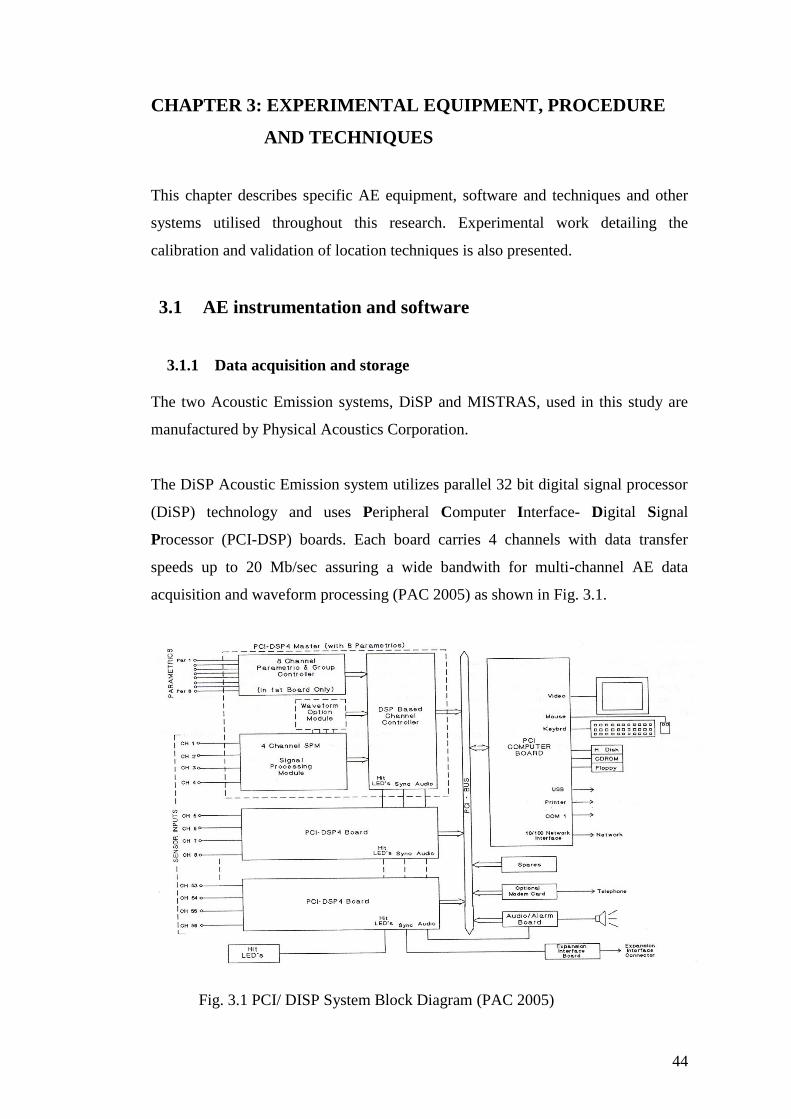
44
CHAPTER 3: EXPERIMENTAL EQUIPMENT, PROCEDURE
AND TECHNIQUES
This chapter describes specific AE equipment, software and techniques and other
systems utilised throughout this research. Experimental work detailing the
calibration and validation of location techniques is also presented.
3.1 AE instrumentation and software
3.1.1 Data acquisition and storage
The two Acoustic Emission systems, DiSP and MISTRAS, used in this study are
manufactured by Physical Acoustics Corporation.
The DiSP Acoustic Emission system utilizes parallel 32 bit digital signal processor
(DiSP) technology and uses Peripheral Computer Interface- Digital Signal
Processor (PCI-DSP) boards. Each board carries 4 channels with data transfer
speeds up to 20 Mb/sec assuring a wide bandwith for multi-channel AE data
acquisition and waveform processing (PAC 2005) as shown in Fig. 3.1.
Fig. 3.1 PCI/ DISP System Block Diagram (PAC 2005)
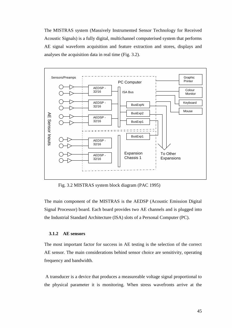
45
The MISTRAS system (Massively Instrumented Sensor Technology for Received
Acoustic Signals) is a fully digital, multichannel computerised system that performs
AE signal waveform acquisition and feature extraction and stores, displays and
analyses the acquisition data in real time (Fig. 3.2).
Fig. 3.2 MISTRAS system block diagram (PAC 1995)
The main component of the MISTRAS is the AEDSP (Acoustic Emission Digital
Signal Processor) board. Each board provides two AE channels and is plugged into
the Industrial Standard Architecture (ISA) slots of a Personal Computer (PC).
3.1.2 AE sensors
The most important factor for success in AE testing is the selection of the correct
AE sensor. The main considerations behind sensor choice are sensitivity, operating
frequency and bandwidth.
A transducer is a device that produces a measureable voltage signal proportional to
the physical parameter it is monitoring. When stress wavefronts arrive at the
AEDSP - 32/16
AEDSP - 32/16
AEDSP - 32/16
AEDSP - 32/16
AEDSP - 32/16
BusExp1
BusExp2
BusExpN
BusExp1
PC Computer
ISA Bus
Graphic Printer
Colour Monitor
Keyboard
Mouse
Sensors/Preamps
AE
Se
nso
r Inpu
ts
Expansion Chassis 1
To Other Expansions
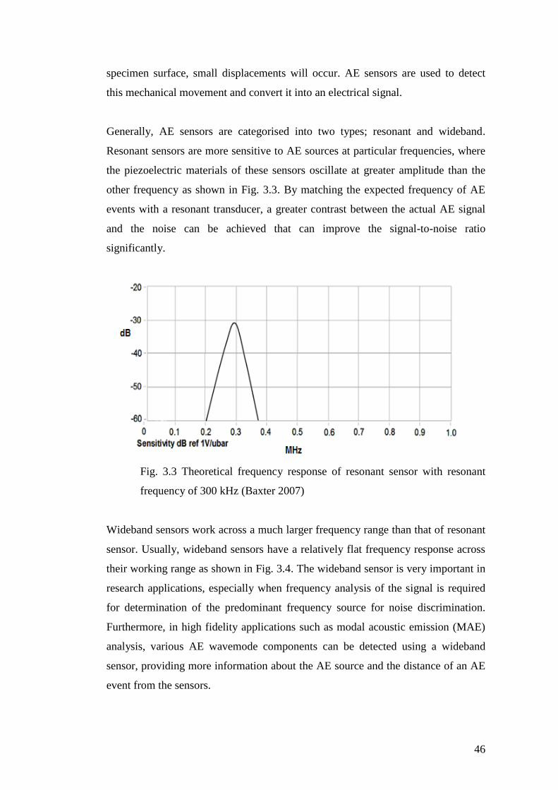
46
specimen surface, small displacements will occur. AE sensors are used to detect
this mechanical movement and convert it into an electrical signal.
Generally, AE sensors are categorised into two types; resonant and wideband.
Resonant sensors are more sensitive to AE sources at particular frequencies, where
the piezoelectric materials of these sensors oscillate at greater amplitude than the
other frequency as shown in Fig. 3.3. By matching the expected frequency of AE
events with a resonant transducer, a greater contrast between the actual AE signal
and the noise can be achieved that can improve the signal-to-noise ratio
significantly.
Fig. 3.3 Theoretical frequency response of resonant sensor with resonant
frequency of 300 kHz (Baxter 2007)
Wideband sensors work across a much larger frequency range than that of resonant
sensor. Usually, wideband sensors have a relatively flat frequency response across
their working range as shown in Fig. 3.4. The wideband sensor is very important in
research applications, especially when frequency analysis of the signal is required
for determination of the predominant frequency source for noise discrimination.
Furthermore, in high fidelity applications such as modal acoustic emission (MAE)
analysis, various AE wavemode components can be detected using a wideband
sensor, providing more information about the AE source and the distance of an AE
event from the sensors.
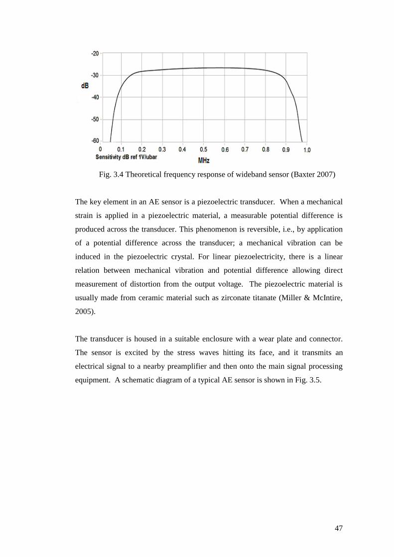
47
Fig. 3.4 Theoretical frequency response of wideband sensor (Baxter 2007)
The key element in an AE sensor is a piezoelectric transducer. When a mechanical
strain is applied in a piezoelectric material, a measurable potential difference is
produced across the transducer. This phenomenon is reversible, i.e., by application
of a potential difference across the transducer; a mechanical vibration can be
induced in the piezoelectric crystal. For linear piezoelectricity, there is a linear
relation between mechanical vibration and potential difference allowing direct
measurement of distortion from the output voltage. The piezoelectric material is
usually made from ceramic material such as zirconate titanate (Miller & McIntire,
2005).
The transducer is housed in a suitable enclosure with a wear plate and connector.
The sensor is excited by the stress waves hitting its face, and it transmits an
electrical signal to a nearby preamplifier and then onto the main signal processing
equipment. A schematic diagram of a typical AE sensor is shown in Fig. 3.5.
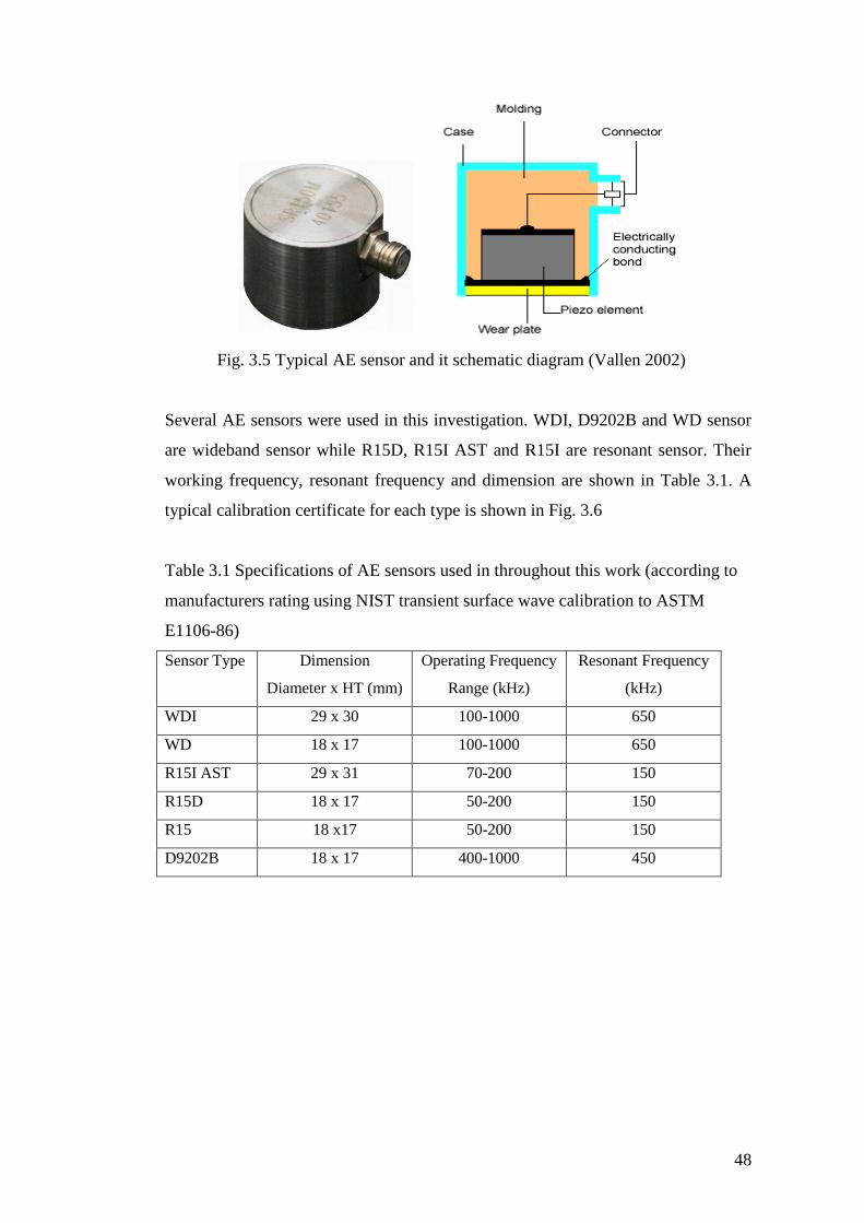
48
Fig. 3.5 Typical AE sensor and it schematic diagram (Vallen 2002)
Several AE sensors were used in this investigation. WDI, D9202B and WD sensor
are wideband sensor while R15D, R15I AST and R15I are resonant sensor. Their
working frequency, resonant frequency and dimension are shown in Table 3.1. A
typical calibration certificate for each type is shown in Fig. 3.6
Table 3.1 Specifications of AE sensors used in throughout this work (according to
manufacturers rating using NIST transient surface wave calibration to ASTM
E1106-86)
Sensor Type Dimension
Diameter x HT (mm)
Operating Frequency
Range (kHz)
Resonant Frequency
(kHz)
WDI 29 x 30 100-1000 650
WD 18 x 17 100-1000 650
R15I AST 29 x 31 70-200 150
R15D 18 x 17 50-200 150
R15 18 x17 50-200 150
D9202B 18 x 17 400-1000 450
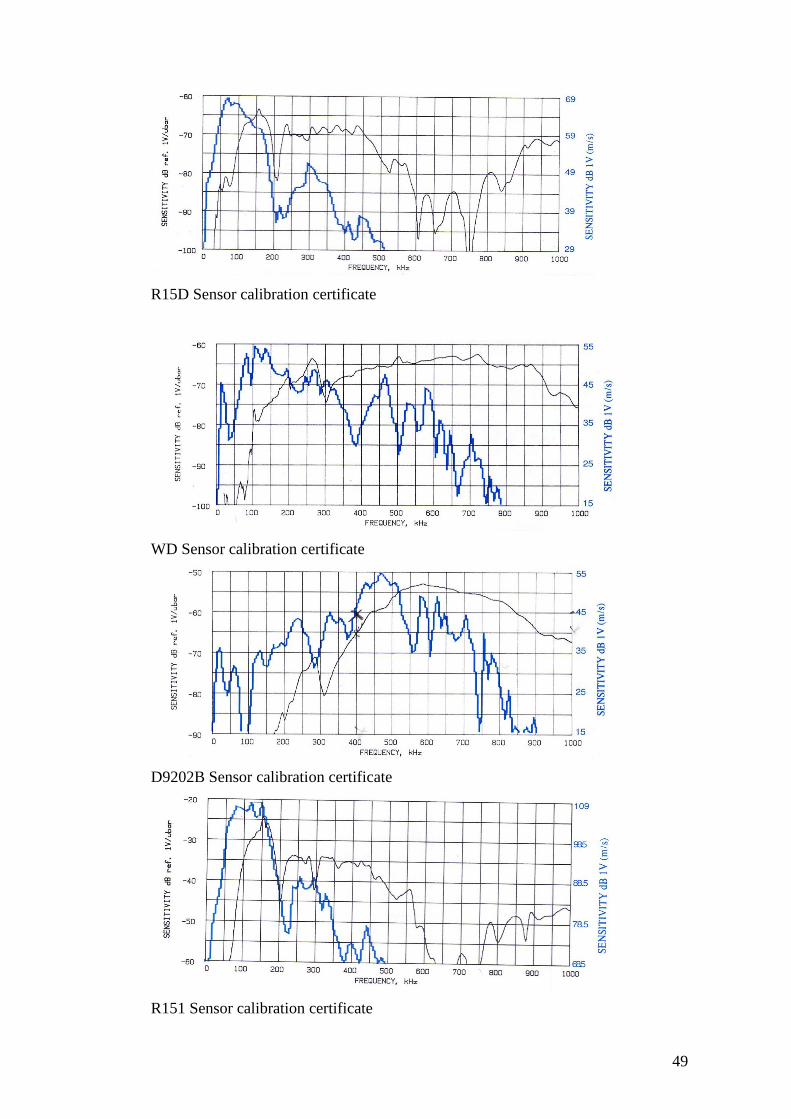
49
R15D Sensor calibration certificate
WD Sensor calibration certificate
D9202B Sensor calibration certificate
R151 Sensor calibration certificate
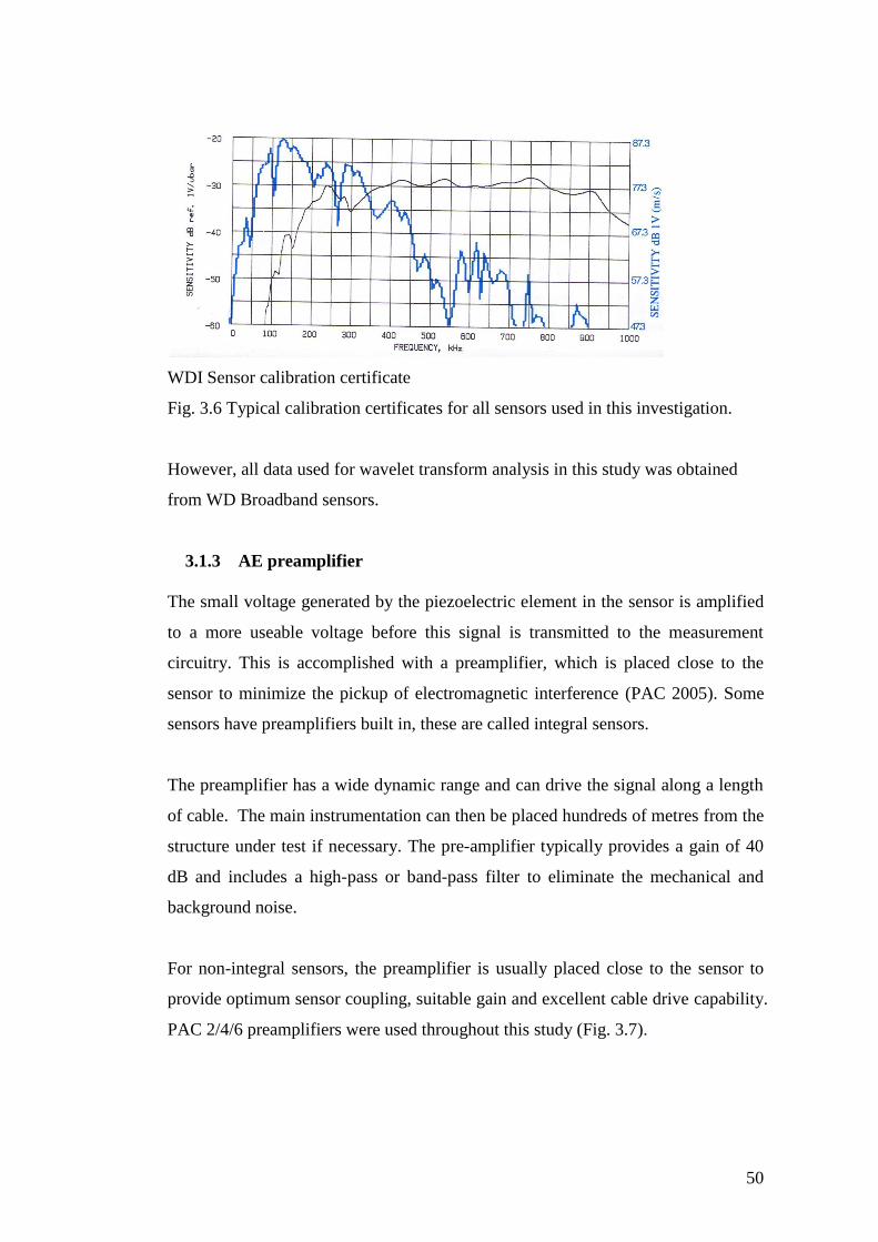
50
WDI Sensor calibration certificate
Fig. 3.6 Typical calibration certificates for all sensors used in this investigation.
However, all data used for wavelet transform analysis in this study was obtained
from WD Broadband sensors.
3.1.3 AE preamplifier
The small voltage generated by the piezoelectric element in the sensor is amplified
to a more useable voltage before this signal is transmitted to the measurement
circuitry. This is accomplished with a preamplifier, which is placed close to the
sensor to minimize the pickup of electromagnetic interference (PAC 2005). Some
sensors have preamplifiers built in, these are called integral sensors.
The preamplifier has a wide dynamic range and can drive the signal along a length
of cable. The main instrumentation can then be placed hundreds of metres from the
structure under test if necessary. The pre-amplifier typically provides a gain of 40
dB and includes a high-pass or band-pass filter to eliminate the mechanical and
background noise.
For non-integral sensors, the preamplifier is usually placed close to the sensor to
provide optimum sensor coupling, suitable gain and excellent cable drive capability.
PAC 2/4/6 preamplifiers were used throughout this study (Fig. 3.7).
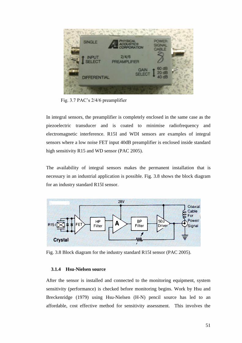
51
Fig. 3.7 PAC’s 2/4/6 preamplifier
In integral sensors, the preamplifier is completely enclosed in the same case as the
piezoelectric transducer and is coated to minimise radiofrequency and
electromagnetic interference. R15I and WDI sensors are examples of integral
sensors where a low noise FET input 40dB preamplifier is enclosed inside standard
high sensitivity R15 and WD sensor (PAC 2005).
The availability of integral sensors makes the permanent installation that is
necessary in an industrial application is possible. Fig. 3.8 shows the block diagram
for an industry standard R15I sensor.
Fig. 3.8 Block diagram for the industry standard R15I sensor (PAC 2005).
3.1.4 Hsu-Nielsen source
After the sensor is installed and connected to the monitoring equipment, system
sensitivity (performance) is checked before monitoring begins. Work by Hsu and
Breckenridge (1979) using Hsu-Nielsen (H-N) pencil source has led to an
affordable, cost effective method for sensitivity assessment. This involves the
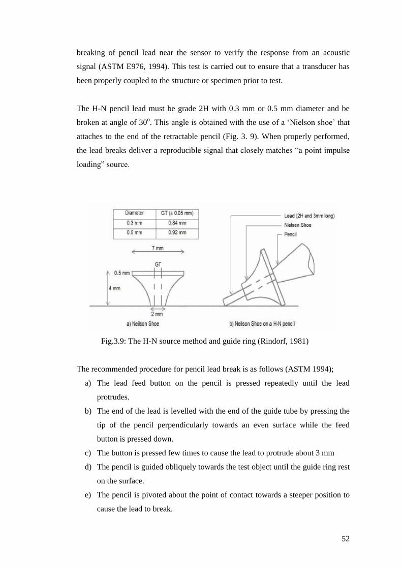
52
breaking of pencil lead near the sensor to verify the response from an acoustic
signal (ASTM E976, 1994). This test is carried out to ensure that a transducer has
been properly coupled to the structure or specimen prior to test.
The H-N pencil lead must be grade 2H with 0.3 mm or 0.5 mm diameter and be
broken at angle of 30o. This angle is obtained with the use of a ‘Nielson shoe’ that
attaches to the end of the retractable pencil (Fig. 3. 9). When properly performed,
the lead breaks deliver a reproducible signal that closely matches “a point impulse
loading” source.
Fig.3.9: The H-N source method and guide ring (Rindorf, 1981)
The recommended procedure for pencil lead break is as follows (ASTM 1994);
a) The lead feed button on the pencil is pressed repeatedly until the lead
protrudes.
b) The end of the lead is levelled with the end of the guide tube by pressing the
tip of the pencil perpendicularly towards an even surface while the feed
button is pressed down.
c) The button is pressed few times to cause the lead to protrude about 3 mm
d) The pencil is guided obliquely towards the test object until the guide ring rest
on the surface.
e) The pencil is pivoted about the point of contact towards a steeper position to
cause the lead to break.
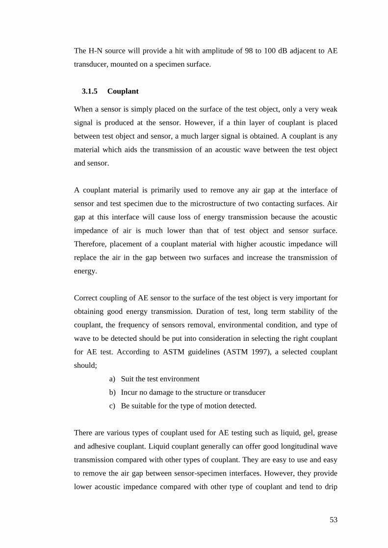
53
The H-N source will provide a hit with amplitude of 98 to 100 dB adjacent to AE
transducer, mounted on a specimen surface.
3.1.5 Couplant
When a sensor is simply placed on the surface of the test object, only a very weak
signal is produced at the sensor. However, if a thin layer of couplant is placed
between test object and sensor, a much larger signal is obtained. A couplant is any
material which aids the transmission of an acoustic wave between the test object
and sensor.
A couplant material is primarily used to remove any air gap at the interface of
sensor and test specimen due to the microstructure of two contacting surfaces. Air
gap at this interface will cause loss of energy transmission because the acoustic
impedance of air is much lower than that of test object and sensor surface.
Therefore, placement of a couplant material with higher acoustic impedance will
replace the air in the gap between two surfaces and increase the transmission of
energy.
Correct coupling of AE sensor to the surface of the test object is very important for
obtaining good energy transmission. Duration of test, long term stability of the
couplant, the frequency of sensors removal, environmental condition, and type of
wave to be detected should be put into consideration in selecting the right couplant
for AE test. According to ASTM guidelines (ASTM 1997), a selected couplant
should;
a) Suit the test environment
b) Incur no damage to the structure or transducer
c) Be suitable for the type of motion detected.
There are various types of couplant used for AE testing such as liquid, gel, grease
and adhesive couplant. Liquid couplant generally can offer good longitudinal wave
transmission compared with other types of couplant. They are easy to use and easy
to remove the air gap between sensor-specimen interfaces. However, they provide
lower acoustic impedance compared with other type of couplant and tend to drip
54
due to low viscosity. Therefore, they are not suitable for any vertical mounting
application as this encourages loss of the couplant layer with time.
Grease based couplants have much higher viscosity than gels or liquids and
therefore are more suitable for rougher surface application. Brown grease is
predominantly used in this investigation. This type of couplant allows lateral sensor
movement to encourage displacement of trapped air (Theobald et. al 2008).
Furthermore, if well clamped, grease offers better long-term stability than gels and
liquids and generally does not damage the surface. However, due to high viscosity
of grease couplant, application of force on the sensor is required to remove all the
trapped air, a mounting fixture is used to meet this purpose.
Adhesive agent can also be used as a couplant. If applied on a clean flat surface, an
adhesive agent can provide better transmission for both longitudinal and shear wave
if correctly applied. This type of couplant is ideal for the applications that need
absolute coupling and sensor stability such as DeltaT source location. The most
common adhesive agents used in AE testing are cyanoacrylate and silicon rubber
compound.
Silicone rubber compound has also been used in this work because it can be applied
as a fluid to achieved a thin layer, bubble free couplant and at the same time
provide a permanent bond on the structure under test. This thin layer can provide
excellent sound transmission which is comparable with greased based couplant but
with a relatively strong bond (Theobald et. al. 2008). Furthermore, silicone rubber
compound also works very well on rough surfaces and has good resistance to bond
failure if surface movement might occur during the test and therefore is suitable for
vertical mounting application. This type of bond enables easier sensor removal after
use with lower risk of sensor damage compared with cyanoacrylate bond.
3.1.6 Sensor mounting
Sensor mounting fixtures are necessary to hold the sensor in a fixed position when
the non-adhesive couplant is used. Typically, when the sensor is coupled to the test
piece, it is secured with tape or a magnetic hold-down device (together with either a
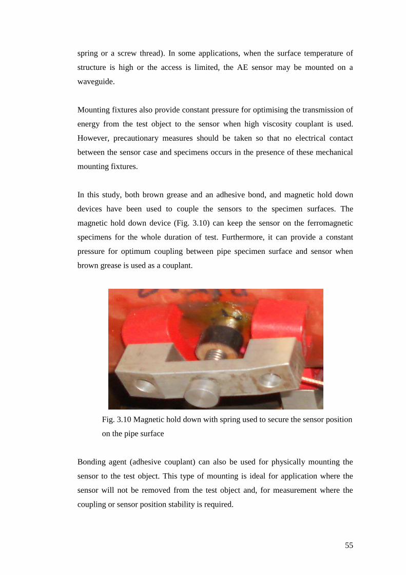
55
spring or a screw thread). In some applications, when the surface temperature of
structure is high or the access is limited, the AE sensor may be mounted on a
waveguide.
Mounting fixtures also provide constant pressure for optimising the transmission of
energy from the test object to the sensor when high viscosity couplant is used.
However, precautionary measures should be taken so that no electrical contact
between the sensor case and specimens occurs in the presence of these mechanical
mounting fixtures.
In this study, both brown grease and an adhesive bond, and magnetic hold down
devices have been used to couple the sensors to the specimen surfaces. The
magnetic hold down device (Fig. 3.10) can keep the sensor on the ferromagnetic
specimens for the whole duration of test. Furthermore, it can provide a constant
pressure for optimum coupling between pipe specimen surface and sensor when
brown grease is used as a couplant.
Fig. 3.10 Magnetic hold down with spring used to secure the sensor position
on the pipe surface
Bonding agent (adhesive couplant) can also be used for physically mounting the
sensor to the test object. This type of mounting is ideal for application where the
sensor will not be removed from the test object and, for measurement where the
coupling or sensor position stability is required.
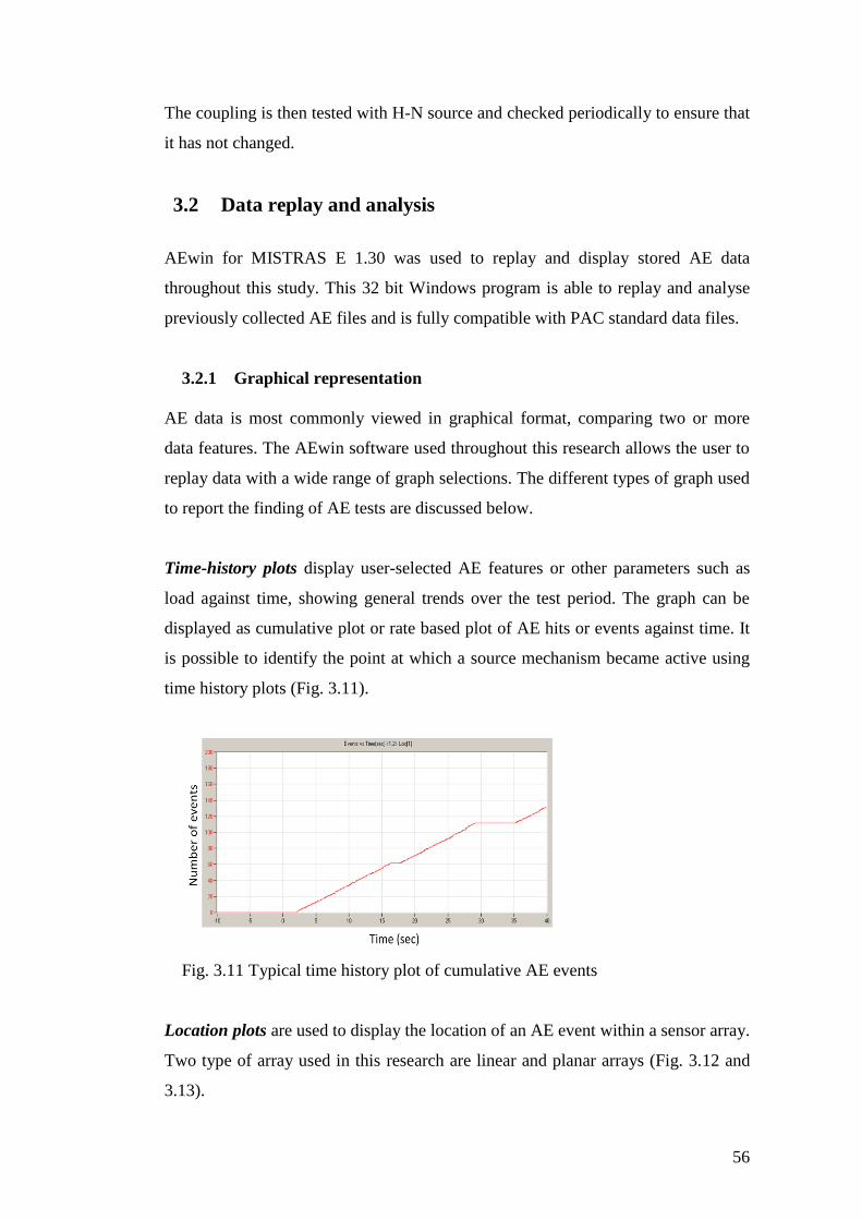
56
The coupling is then tested with H-N source and checked periodically to ensure that
it has not changed.
3.2 Data replay and analysis
AEwin for MISTRAS E 1.30 was used to replay and display stored AE data
throughout this study. This 32 bit Windows program is able to replay and analyse
previously collected AE files and is fully compatible with PAC standard data files.
3.2.1 Graphical representation
AE data is most commonly viewed in graphical format, comparing two or more
data features. The AEwin software used throughout this research allows the user to
replay data with a wide range of graph selections. The different types of graph used
to report the finding of AE tests are discussed below.
Time-history plots display user-selected AE features or other parameters such as
load against time, showing general trends over the test period. The graph can be
displayed as cumulative plot or rate based plot of AE hits or events against time. It
is possible to identify the point at which a source mechanism became active using
time history plots (Fig. 3.11).
Fig. 3.11 Typical time history plot of cumulative AE events
Location plots are used to display the location of an AE event within a sensor array.
Two type of array used in this research are linear and planar arrays (Fig. 3.12 and
3.13).
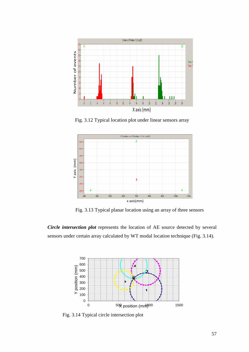
57
Fig. 3.12 Typical location plot under linear sensors array
Fig. 3.13 Typical planar location using an array of three sensors
Circle intersection plot represents the location of AE source detected by several
sensors under certain array calculated by WT modal location technique (Fig. 3.14).
Fig. 3.14 Typical circle intersection plot
0
100
200
300
400
500
600
700
0 500 1000 1500
Y p
ositio
n (
mm
)
X position (mm)
1
2
3
4
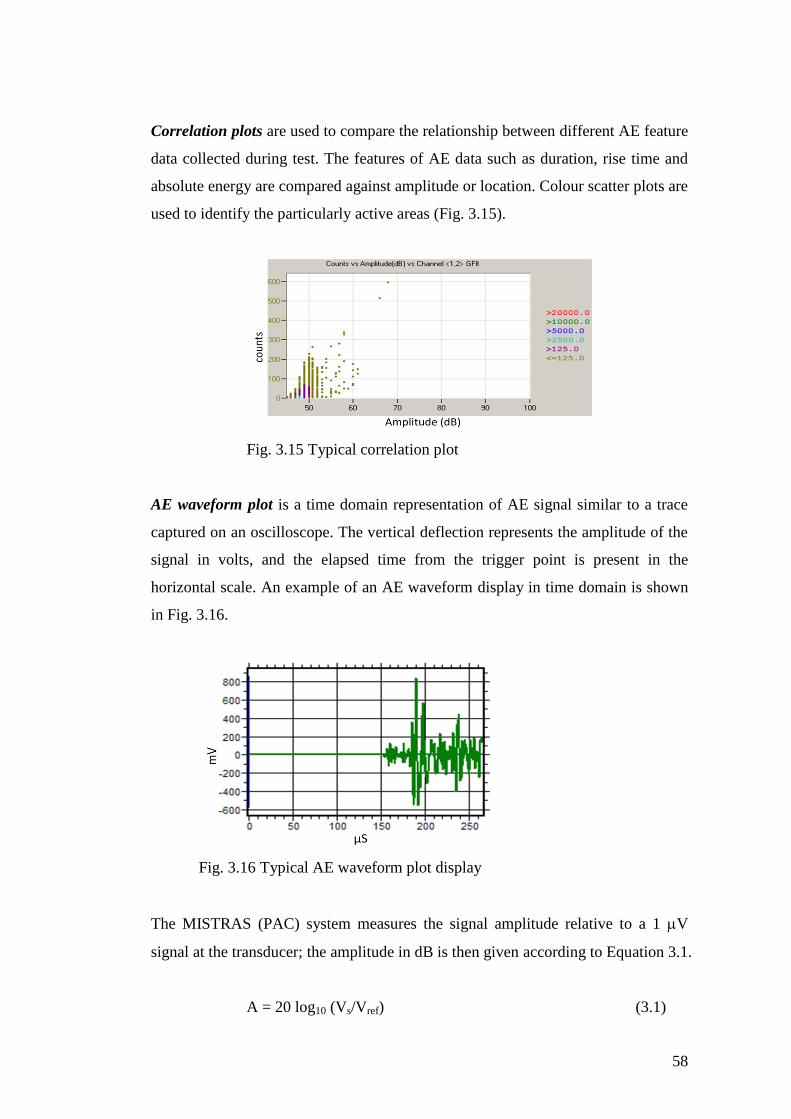
58
Correlation plots are used to compare the relationship between different AE feature
data collected during test. The features of AE data such as duration, rise time and
absolute energy are compared against amplitude or location. Colour scatter plots are
used to identify the particularly active areas (Fig. 3.15).
Fig. 3.15 Typical correlation plot
AE waveform plot is a time domain representation of AE signal similar to a trace
captured on an oscilloscope. The vertical deflection represents the amplitude of the
signal in volts, and the elapsed time from the trigger point is present in the
horizontal scale. An example of an AE waveform display in time domain is shown
in Fig. 3.16.
Fig. 3.16 Typical AE waveform plot display
The MISTRAS (PAC) system measures the signal amplitude relative to a 1 V
signal at the transducer; the amplitude in dB is then given according to Equation 3.1.
A = 20 log10 (Vs/Vref) (3.1)
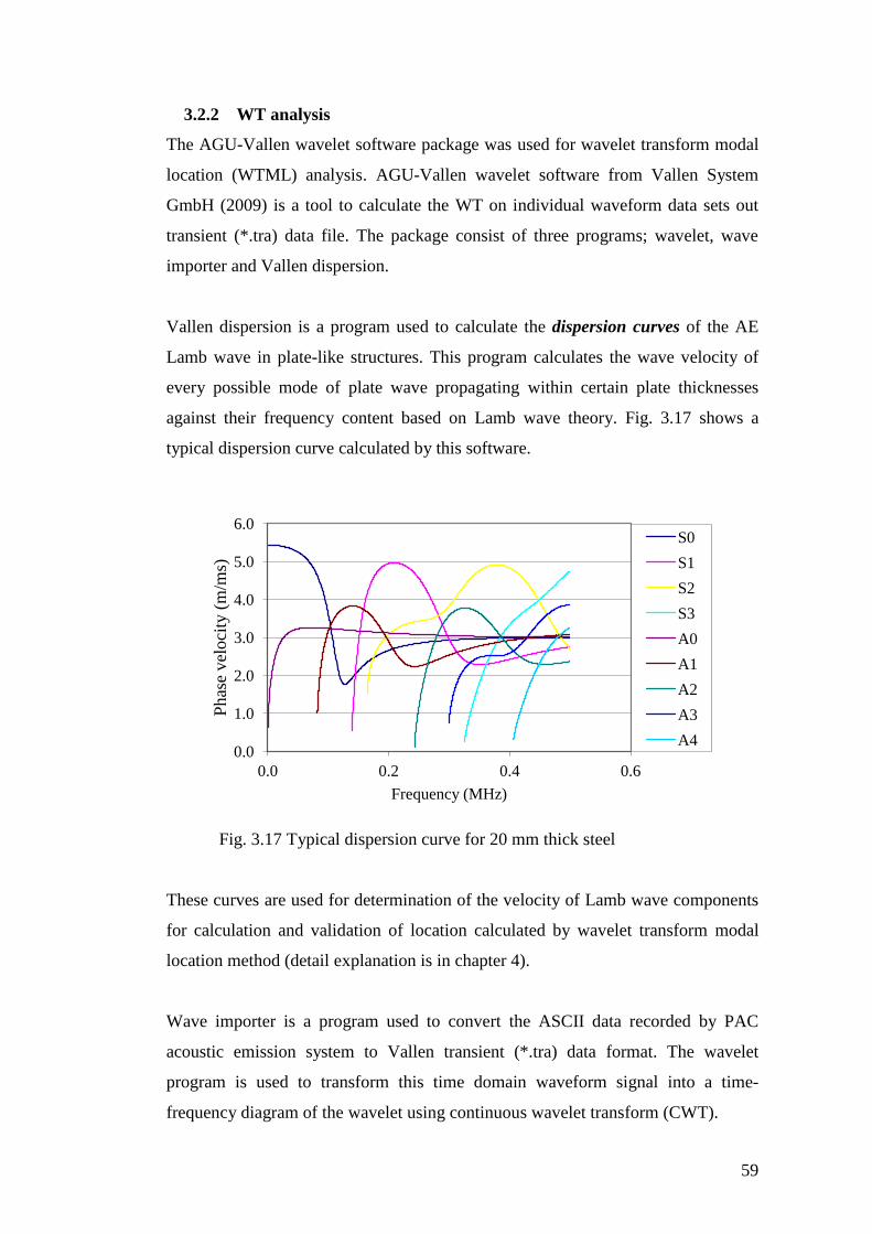
59
3.2.2 WT analysis
The AGU-Vallen wavelet software package was used for wavelet transform modal
location (WTML) analysis. AGU-Vallen wavelet software from Vallen System
GmbH (2009) is a tool to calculate the WT on individual waveform data sets out
transient (*.tra) data file. The package consist of three programs; wavelet, wave
importer and Vallen dispersion.
Vallen dispersion is a program used to calculate the dispersion curves of the AE
Lamb wave in plate-like structures. This program calculates the wave velocity of
every possible mode of plate wave propagating within certain plate thicknesses
against their frequency content based on Lamb wave theory. Fig. 3.17 shows a
typical dispersion curve calculated by this software.
Fig. 3.17 Typical dispersion curve for 20 mm thick steel
These curves are used for determination of the velocity of Lamb wave components
for calculation and validation of location calculated by wavelet transform modal
location method (detail explanation is in chapter 4).
Wave importer is a program used to convert the ASCII data recorded by PAC
acoustic emission system to Vallen transient (*.tra) data format. The wavelet
program is used to transform this time domain waveform signal into a time-
frequency diagram of the wavelet using continuous wavelet transform (CWT).
0.0
1.0
2.0
3.0
4.0
5.0
6.0
0.0 0.2 0.4 0.6
Phas
e vel
oci
ty (
m/m
s)
Frequency (MHz)
S0
S1
S2
S3
A0
A1
A2
A3
A4
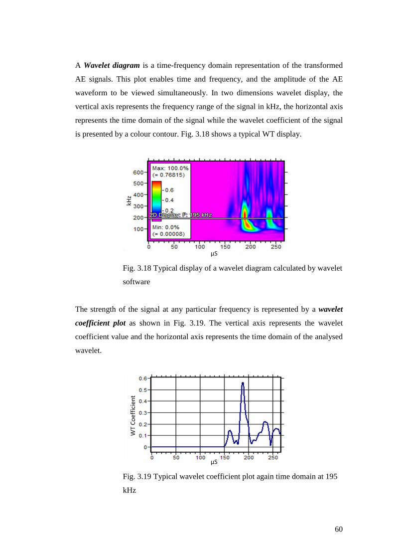
60
A Wavelet diagram is a time-frequency domain representation of the transformed
AE signals. This plot enables time and frequency, and the amplitude of the AE
waveform to be viewed simultaneously. In two dimensions wavelet display, the
vertical axis represents the frequency range of the signal in kHz, the horizontal axis
represents the time domain of the signal while the wavelet coefficient of the signal
is presented by a colour contour. Fig. 3.18 shows a typical WT display.
Fig. 3.18 Typical display of a wavelet diagram calculated by wavelet
software
The strength of the signal at any particular frequency is represented by a wavelet
coefficient plot as shown in Fig. 3.19. The vertical axis represents the wavelet
coefficient value and the horizontal axis represents the time domain of the analysed
wavelet.
Fig. 3.19 Typical wavelet coefficient plot again time domain at 195
kHz
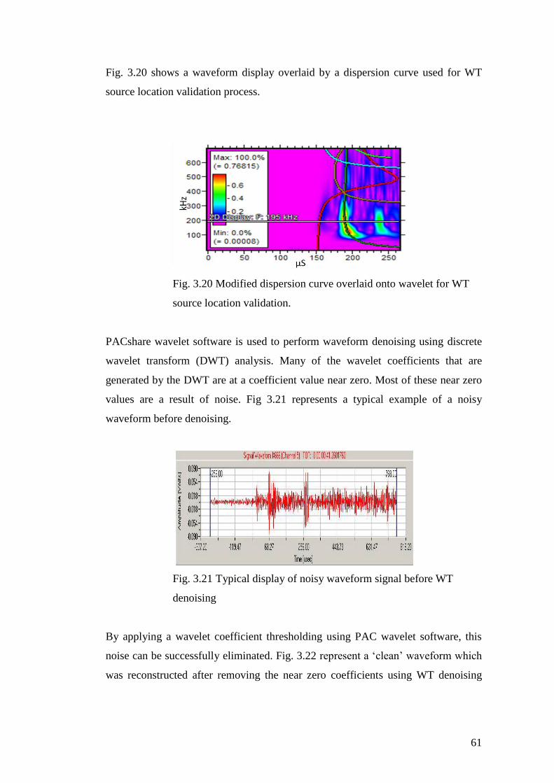
61
Fig. 3.20 shows a waveform display overlaid by a dispersion curve used for WT
source location validation process.
Fig. 3.20 Modified dispersion curve overlaid onto wavelet for WT
source location validation.
PACshare wavelet software is used to perform waveform denoising using discrete
wavelet transform (DWT) analysis. Many of the wavelet coefficients that are
generated by the DWT are at a coefficient value near zero. Most of these near zero
values are a result of noise. Fig 3.21 represents a typical example of a noisy
waveform before denoising.
Fig. 3.21 Typical display of noisy waveform signal before WT
denoising
By applying a wavelet coefficient thresholding using PAC wavelet software, this
noise can be successfully eliminated. Fig. 3.22 represent a ‘clean’ waveform which
was reconstructed after removing the near zero coefficients using WT denoising
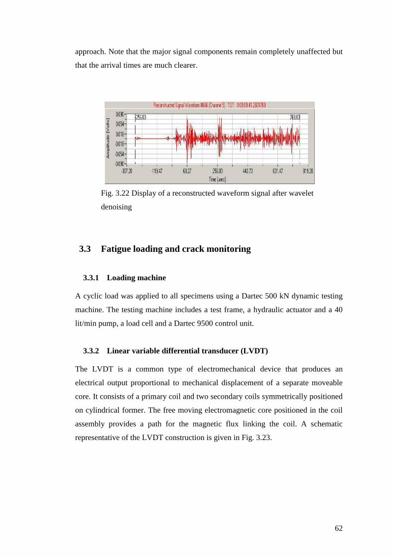
62
approach. Note that the major signal components remain completely unaffected but
that the arrival times are much clearer.
Fig. 3.22 Display of a reconstructed waveform signal after wavelet
denoising
3.3 Fatigue loading and crack monitoring
3.3.1 Loading machine
A cyclic load was applied to all specimens using a Dartec 500 kN dynamic testing
machine. The testing machine includes a test frame, a hydraulic actuator and a 40
lit/min pump, a load cell and a Dartec 9500 control unit.
3.3.2 Linear variable differential transducer (LVDT)
The LVDT is a common type of electromechanical device that produces an
electrical output proportional to mechanical displacement of a separate moveable
core. It consists of a primary coil and two secondary coils symmetrically positioned
on cylindrical former. The free moving electromagnetic core positioned in the coil
assembly provides a path for the magnetic flux linking the coil. A schematic
representative of the LVDT construction is given in Fig. 3.23.
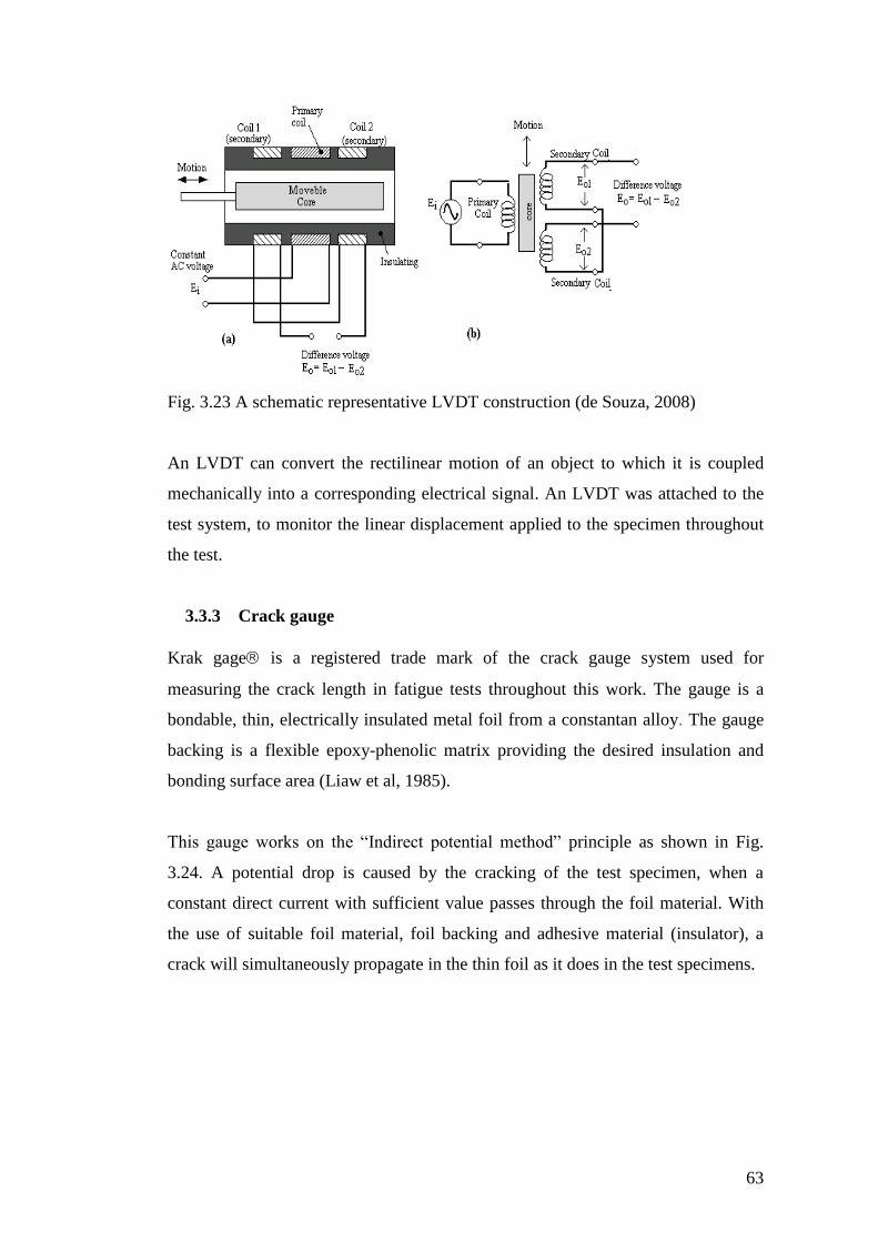
63
Fig. 3.23 A schematic representative LVDT construction (de Souza, 2008)
An LVDT can convert the rectilinear motion of an object to which it is coupled
mechanically into a corresponding electrical signal. An LVDT was attached to the
test system, to monitor the linear displacement applied to the specimen throughout
the test.
3.3.3 Crack gauge
Krak gage is a registered trade mark of the crack gauge system used for
measuring the crack length in fatigue tests throughout this work. The gauge is a
bondable, thin, electrically insulated metal foil from a constantan alloy. The gauge
backing is a flexible epoxy-phenolic matrix providing the desired insulation and
bonding surface area (Liaw et al, 1985).
This gauge works on the “Indirect potential method” principle as shown in Fig.
3.24. A potential drop is caused by the cracking of the test specimen, when a
constant direct current with sufficient value passes through the foil material. With
the use of suitable foil material, foil backing and adhesive material (insulator), a
crack will simultaneously propagate in the thin foil as it does in the test specimens.
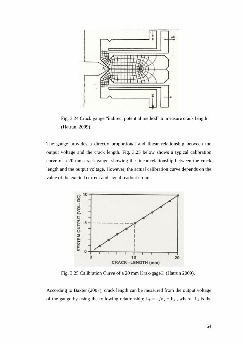
64
Fig. 3.24 Crack gauge “indirect potential method” to measure crack length
(Hatrun, 2009).
The gauge provides a directly proportional and linear relationship between the
output voltage and the crack length. Fig. 3.25 below shows a typical calibration
curve of a 20 mm crack gauge, showing the linear relationship between the crack
length and the output voltage. However, the actual calibration curve depends on the
value of the excited current and signal readout circuit.
Fig. 3.25 Calibration Curve of a 20 mm Krak-gage (Hatrun 2009).
According to Baxter (2007), crack length can be measured from the output voltage
of the gauge by using the following relationship; Lk = akVk + bk , where Lk is the
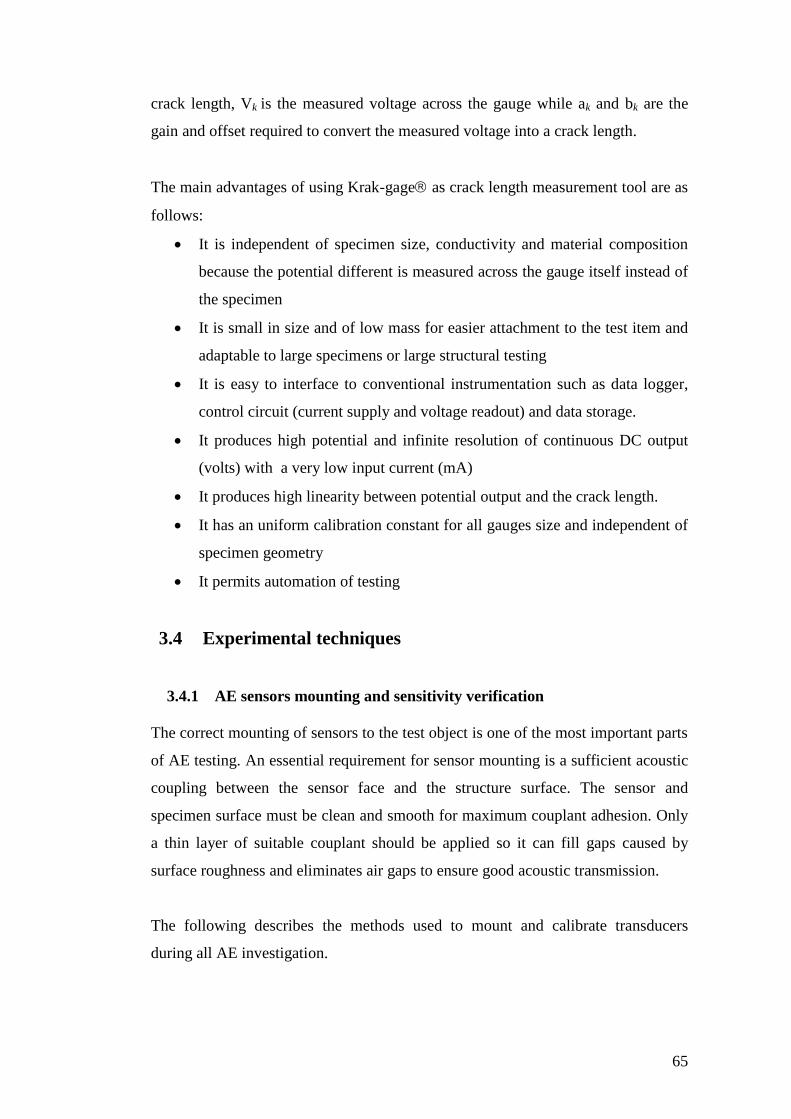
65
crack length, Vk is the measured voltage across the gauge while ak and bk are the
gain and offset required to convert the measured voltage into a crack length.
The main advantages of using Krak-gage as crack length measurement tool are as
follows:
It is independent of specimen size, conductivity and material composition
because the potential different is measured across the gauge itself instead of
the specimen
It is small in size and of low mass for easier attachment to the test item and
adaptable to large specimens or large structural testing
It is easy to interface to conventional instrumentation such as data logger,
control circuit (current supply and voltage readout) and data storage.
It produces high potential and infinite resolution of continuous DC output
(volts) with a very low input current (mA)
It produces high linearity between potential output and the crack length.
It has an uniform calibration constant for all gauges size and independent of
specimen geometry
It permits automation of testing
3.4 Experimental techniques
3.4.1 AE sensors mounting and sensitivity verification
The correct mounting of sensors to the test object is one of the most important parts
of AE testing. An essential requirement for sensor mounting is a sufficient acoustic
coupling between the sensor face and the structure surface. The sensor and
specimen surface must be clean and smooth for maximum couplant adhesion. Only
a thin layer of suitable couplant should be applied so it can fill gaps caused by
surface roughness and eliminates air gaps to ensure good acoustic transmission.
The following describes the methods used to mount and calibrate transducers
during all AE investigation.
66
a) The specimen surface for sensor mounting is cleaned to remove all
irregularities to ensure maximum area contact between sensor and
surface. This is for optimising the AE transfer coupling. This usually
takes the form of light sanding for normal surfaces. For paint coated
specimen, filing is used to remove the paint from the surface.
b) A couplant is applied to ensure the optimum transmission of AE
signal between specimen and sensor. Brown grease is predominantly
used in this investigation especially for the test carried out on the
non flat surface such as on pipe specimen whereas silicone rubber
compound is also used for flat surface specimens.
c) The sensor is placed on the structure surface and rotated slightly to
ensure an adequate layer of couplant covers the surface of the sensor.
The sensor is secured by a magnetic clamp for the whole test
duration, which ensures that a constant pressure is applied between
the sensor and the test specimen.
d) A cable is attached to the sensor and to the corresponding channel at
the rear of the AE data acquisition system. The cable is secured to
ensure that no strain occurs in the cable during monitoring.
e) The sensitivity of the mounted sensor is verified using an artificial
source (H-N source). Pencil lead fracture is performed adjacent to
the sensor and the AE signal is recorded. A well mounted sensor
should record a signal with amplitude of 98-100 dB. If a sensors
response is below 98dB, the sensor has to be remounted and
rechecked again. If the response is still low, the cabling is checked
by performing a pencil lead break on the face of the sensor. The
cable should be replaced if the signal response is less than 100dB. If
the signal response still does not meet those criteria after cable
replacement, then the sensor should be replaced.
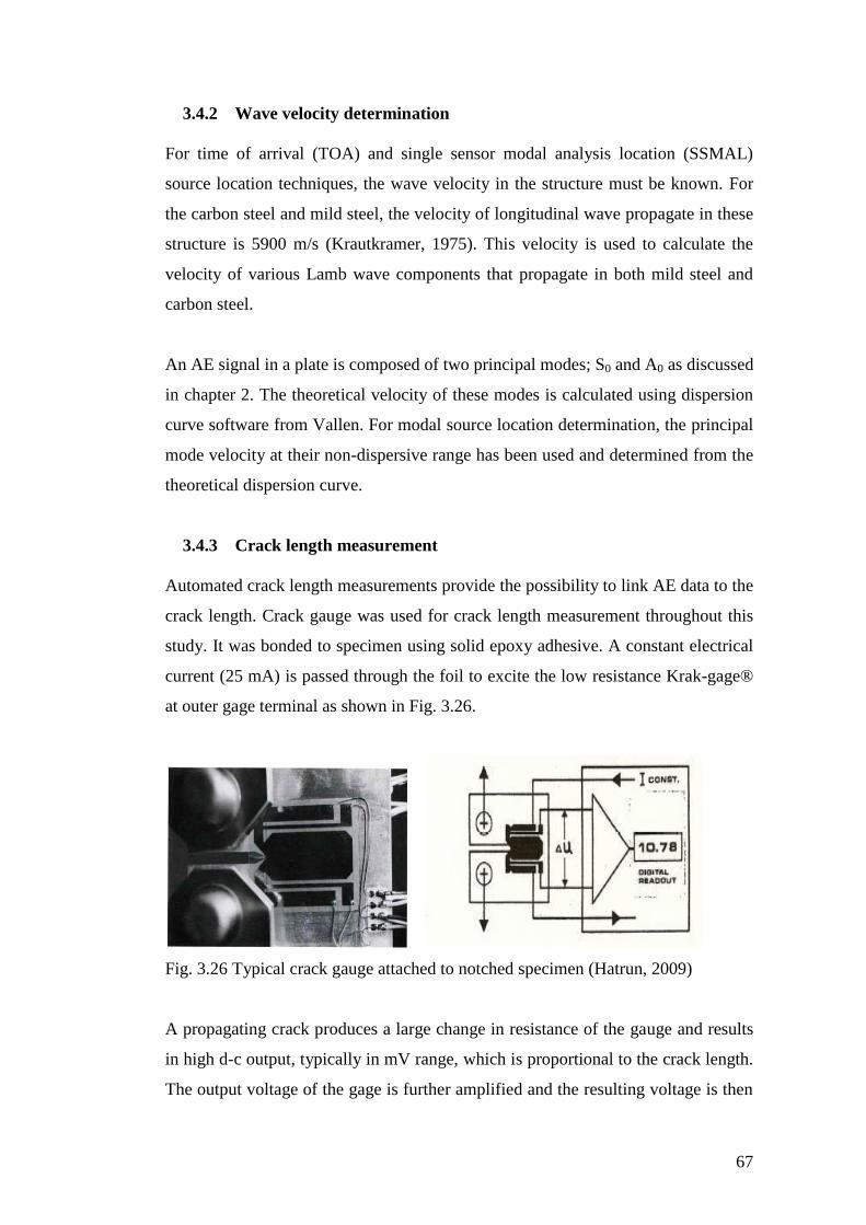
67
3.4.2 Wave velocity determination
For time of arrival (TOA) and single sensor modal analysis location (SSMAL)
source location techniques, the wave velocity in the structure must be known. For
the carbon steel and mild steel, the velocity of longitudinal wave propagate in these
structure is 5900 m/s (Krautkramer, 1975). This velocity is used to calculate the
velocity of various Lamb wave components that propagate in both mild steel and
carbon steel.
An AE signal in a plate is composed of two principal modes; S0 and A0 as discussed
in chapter 2. The theoretical velocity of these modes is calculated using dispersion
curve software from Vallen. For modal source location determination, the principal
mode velocity at their non-dispersive range has been used and determined from the
theoretical dispersion curve.
3.4.3 Crack length measurement
Automated crack length measurements provide the possibility to link AE data to the
crack length. Crack gauge was used for crack length measurement throughout this
study. It was bonded to specimen using solid epoxy adhesive. A constant electrical
current (25 mA) is passed through the foil to excite the low resistance Krak-gage®
at outer gage terminal as shown in Fig. 3.26.
Fig. 3.26 Typical crack gauge attached to notched specimen (Hatrun, 2009)
A propagating crack produces a large change in resistance of the gauge and results
in high d-c output, typically in mV range, which is proportional to the crack length.
The output voltage of the gage is further amplified and the resulting voltage is then
68
measured using a circuit, the output of which is fed to the data logger to enable
digital data to be stored into computer.
3.4.4 Dye penetrant inspection
Dye penetrant is a non-destructive method used to aid visual inspection by enabling
cracks that have broken to the surface to be readily seen. Dye penetrant testing
works on capillary action where dye liquid with low surface tension penetrates
inside the crack. Red dye penetrant is used in this work to ensure the indications
produce a good contrast with a white developer.
Dye penetrant testing is carried out in accordance with ASTM E 165-95 (2001)
which involve six major steps; pre-cleaning, penetrant application, removal excess
penetrant, application of developer, inspection and post cleaning.
i. Pre cleaning
The surface of the specimen is first cleaned by wiping with tissues damped with
solvent material. This step is carried out to remove any dirt or any loose scale that
may prevent the penetrant from penetrating the crack or may cause false indication.
ii. Application of penetrant
Once the surface is cleaned, the red dye is then applied to the clean surface of the
specimen under test. The red dye is left to remain on the specimen surface for about
an hour. This time is called “dwell time” which provides enough duration for the
penetrant material to soak deep into the fatigue crack and at the same time allows
the excess penetrant to drain out from the surface of the part under test.
iii. Removal of excess penetrant
Excess penetrant is removed from the surface after an hour of penetrant application
by wiping with clean cloth damped with solvent material. This will remove any
trace of excess penetrant material on the specimen surface to avoid false indication
while at the same time leaving penetrant inside the crack.
iv. Application of developer

69
A white developer is applied onto the specimen surface, this draws penetrant from
cracks out onto the surface to form the visible indication. This action is known as
“bleed out”. Any areas that bleed-out reveal the location and orientation of crack
on the surface.
v. Inspection
Inspection of the test surface is carried out one hour after developer application.
This duration is known as developing time, the time required to allow penetrant
inside the crack to blot out onto surface of specimen to form a visible indication.
The length can be measured and the image (picture) captured.
vi. Post cleaning
The test surface is cleaned after the test and recording of defects using the solvent
remover.
The dye penetrant test is used throughout this work to locate the fatigue crack
growth because of the following;
it is a low cost inspection method
test is easy to carry out and does not involve complicated instrumentation
the inspection can be carry out in shorter time and
Results are visible.
3.4.5 DeltaT source location
DeltaT source location is an AE location method based on the different time arrival
at a pair of sensors. It requires a time contour map of the specimen to be
constructed and this provides expected time arrivals regardless of specimen
thickness and geometry. The source location is accomplished by comparing the
actual AE data from the test with the time contour map.
Delta T analysis involves five important step as follows;
i. Determine the area of interest
ii. Construct a calibration grid
iii. Obtain training data
70
iv. Calculate DeltaT map
v. Compare actual data with contour map
Before DeltaT analysis is carried out, the area of interest on in the structure under
test should be first identified. A grid is then constructed around this area. The grid
area should be sufficient to cover the final location of the defect/damage and the
direction of fatigue crack growth. Training data for DeltaT map was obtained by
conducting an H-N source at each node (5 sources per node) of the grid.
A time contour map (which is independent of velocity) is constructed over the area
of interest by analysis of the arrival time delay at pairs of sensors from particular
source locations. Noesis software from PAC and DeltaT software developed by
Baxter et al (2007) has been used for this analysis. The contour map is saved as
data file and gives information of the time delay between pairs sensor at each nodes.
Any crack signal will be processed with DeltaT software (by calculating the time
different at each sensors pairs for any detected events) and then is compared with
contour map.
3.4.6 Triple point filtering analysis
Triple point waveform filtering based source location is achieved by performing
narrow band filtering at the frequency at which S0, A0 and A1 modes propagate at
same velocity. This analysis is carried out to improve the accuracy of TOA source
location by eliminating the timing triggering error.
3.5 Summary
This chapter described the equipment used for AE data acquisition, data replay and
data analysis. Two Acoustic Emission systems, DiSP and MISTRAS, manufactured
by Physical Acoustic Emission were used in laboratory testing. Wide band WD
sensors with working frequency range of 100-1000 kHz were used to detect the
Lamb waves.
AEwin for Mistras E 1.30 was used for replay and displayed the stored data
throughout this study. This software was also used for data feature extraction for
71
characterisation of damage mechanism, data filtering, TOA source location and
triple point waveform filtering source location.
The software utilised for WT analysis was also described. The AGU-Vallen
wavelet software package was used for continuous WT analysis. PACshare wavelet
software from Physical Acoustic Corporation is used to perform waveform
denoising using discrete wavelet transform (DWT) analysis.
Other equipment for monitoring the crack growth in steel plate was also well
explained. Crack gauge and liquid penetrant testing has been used to monitor the
crack length during the fatigue test.
72
CHAPTER 4: DEVEPLOPMENT AND VERIFICATION OF
NOVEL WAVELET TRANSFORM ANALYSIS
AND MODAL LOCATION (WTML)
METHODOLOGY FOR ACCURATE SOURCE
LOCATION AND CRACK SIZING
4.1 Introduction
The AE technique has been used to monitor the integrity of the seam weld of reheat
steam piping in nuclear piping system (IAEA, 2003) and fossil fuel power plant
(Rodgers et al, 1996). Fatigue cracks have been successfully located at the critical
area on fossil power plant piping systems; however other non-destructive testing
(NDT) has been used to evaluate the defect size.
This chapter aims to develop a new AE source location methodology using wavelet
transform analysis (WT), to compare the accuracy of the new proposed method
with time of arrival (TOA) and DeltaT methods, and to seek the possibility of
developing an AE crack length measurement procedure based on WT analysis and
modal location theory.
4.2 AE source location technique ; principles and limitations
Source location is an important feature of AE structural integrity monitoring and
accurate source location requires the application of a series of very important
processes, including; accurate detection and processing of AE signals, event
detection and grouping of AE signals to form an accurate event record, extraction
of critical timing features and assignment of their correct propagation velocity, and
application of the appropriate location algorithm.
4.2.1 Time of arrival (TOA)
Time of arrival (TOA) source location is the most widely used location method and
this is the basis used in most of the commercial AE software. However, other
73
methods such as single sensor modal analysis method (SSMAL) (Pullin 2005),
DeltaT method (Baxter 2007) and Waveform filtering methods (Miller and
McIntire 2005) can also be used. A detailed explanation of source location is
presented in chapter 2.
TOA method is based on time arrival of an AE event at sensors within an array. In
this method, the velocity of wave propagation in the medium is assumed to be
constant and in a direct path. However, due to the noise from the environment, most
of the available commercial AE system use first threshold crossing for measuring
this flight time of the AE signal instead of first hit arrival. Triggering error and time
delay between the first hit arrivals and first threshold crossing will produce an error
in the TOA measurement which may lead to source location inaccuracy. Other
causes of source location inaccuracy include inaccurate sensor location, incorrect
group wave velocity and human error.
4.2.2 DeltaT
The DeltaT method still uses the time of arrival of the signal at the sensor. However,
in the DeltaT method, source location is derived from a user-defined arrival contour
map rather than using a constant wave velocity. The method is described in detail in
chapter 2.
This method was shown to be more accurate than the TOA technique because
velocity and geometry errors are minimised and the effects of boundary reflections
and mode conversion are accounted for. This method is suitable for structural
health monitoring of structures with non uniform geometry such as in aircraft
landing gear (Baxter, 2007).
This method does have its drawbacks however; the map must be constructed before
the actual test for a specific location. The AE signal detected by the system is
compared with the constructed map and therefore the AE data from outside the map
area cannot be analysed. On top of that, the analysis is only valid if the location of
the sensor arrays does not change. Furthermore, since the arrival time for this
location method is also determined by first threshold crossing, time of arrival error
74
due to delay between first hit arrival and first threshold crossing may also lead to
source location inaccuracy.
4.2.3 Single Sensor Modal Analysis Location (SSMAL)
Conventional AE location techniques have mainly utilised the time arrival at first
threshold crossing. An alternative to this conventional technique exploits the
dispersive nature of Lamb waves and is known as modal acoustic emission (MAE)
and the method is described in detail in Chapter 2.
SSMAL is expected to produce better location results compared with TOA method
since the timing error due the arrival delay between first hit arrival and first
threshold crossing is minimised. However, due to dispersion characteristic of
Lamb wave, superposition of A0 mode arrival with other higher order Asymmetry
components will lead to source location inaccuracy due to temporal separation
measurement error.
Temporal separation measurement error in SSMAL can be improved by deploying
time-frequency analysis which can discriminate the content of AE signal instead of
depending on time domain waveform analysis. To the author’s knowledge, this has
not been achieved to date by any other researcher.
4.3 SSMAL with Modified Dispersion Curve
4.3.1 Introduction
According to Lamb wave theory, when acoustic waves propagate within plate-like
structures, their movements are limited by the boundary of the plate. The
propagation of Lamb waves in plate-like structures is characterised by the wave
modes velocity dispersion with frequency content and can be illustrated using
dispersion curves. There are several symmetric and asymmetric AE modes that will
propagate with difference velocities. The temporal separation between the
fundamental symmetric (S0) and asymmetric (A0) mode has been used in SSMAL
for more accurate source location (Pullin 2005). In order to obtained the correct
75
temporal separation between S0 and A0 mode for accurate SSMAL, the arrival of A0
mode should be discriminated from other wave mode that propagate at the velocity
that is close to A0 mode velocity. Modified dispersion curves can be used to
determine the time arrival of these two modes.
The modified dispersion curve used in this study is a plot of the frequency of a
series of Lamb wave modes against their arrival time for known source-to-sensor
distances for a specific plate thickness. Instead of plotting velocity against
frequency (as in the normal dispersion curve), modified dispersion curves display
the frequency content of the signal in vertical axis against arrival time in the
horizontal axis. This modified dispersion curve is then overlaid onto the waveform
signal for evaluating the temporal separation between S0 and A0 modes.
Since both modified dispersion graph and waveform signal have the same
horizontal time axis, the arrival time of the fundamental symmetry and asymmetry
modes in the waveform can be determined by evaluating the arrival time of the
corresponding wave mode in this new (modified) dispersion curve.
4.3.2 Objective of the study
This study has been completed to
i. Investigate the effect of plate thickness on dispersion curves.
ii. Investigate the use of modified dispersion curves to discriminate the
arrival of different asymmetric mode for more accurate SSMAL.
4.3.3 Experimental procedure
A 20 mm thick ASTM 516 gr 70 steel plate measuring 80 mm x 2m and a 4 mm
thick mild steel plate measuring 500 mm x 1500 mm are used in this study. The re
use of plates with different thickness is to study the effect of thickness on the Lamb
wave velocity dispersion. The theoretical dispersion curve for both plates was
calculated using Vallen Dispersion software.
For modified dispersion curves analysis, H-N sources at four known source to
sensor locations on the 20 mm thick ASTM were used in this work. Dispersion
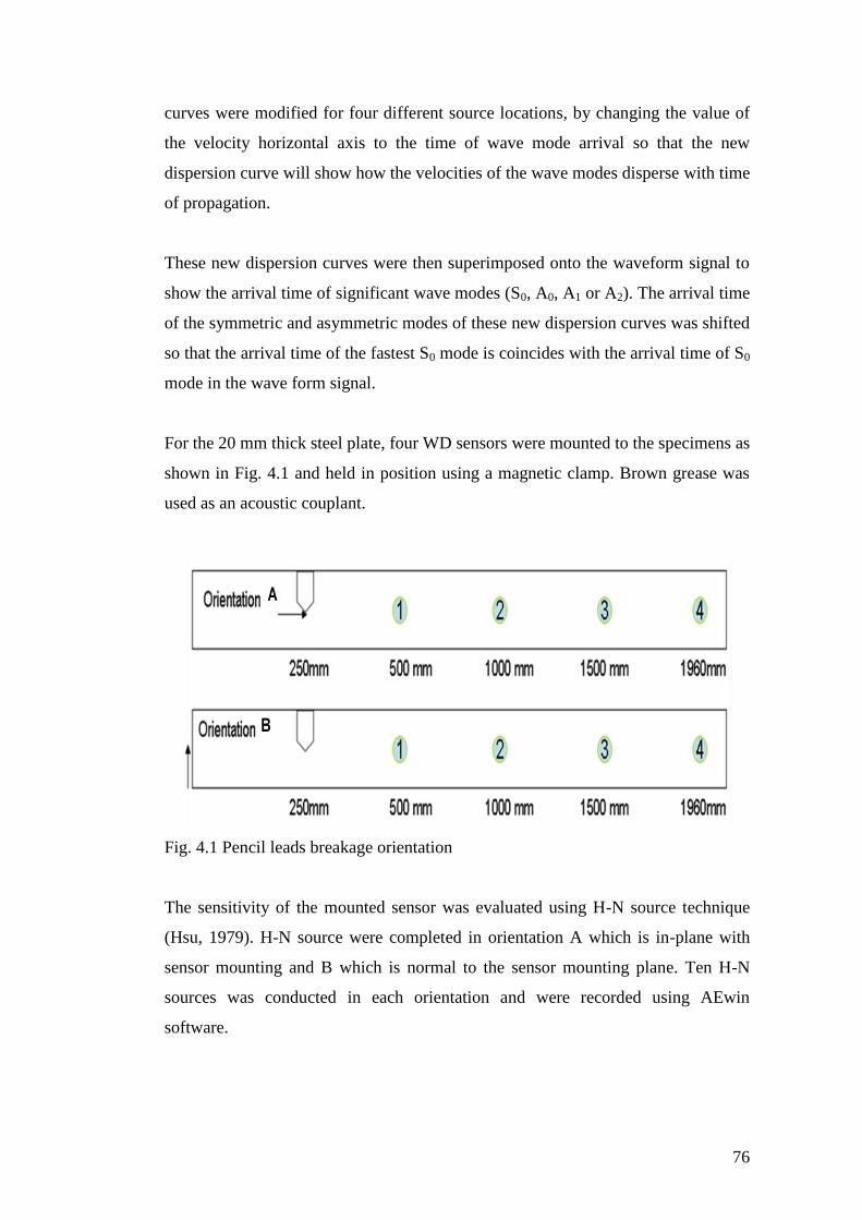
76
curves were modified for four different source locations, by changing the value of
the velocity horizontal axis to the time of wave mode arrival so that the new
dispersion curve will show how the velocities of the wave modes disperse with time
of propagation.
These new dispersion curves were then superimposed onto the waveform signal to
show the arrival time of significant wave modes (S0, A0, A1 or A2). The arrival time
of the symmetric and asymmetric modes of these new dispersion curves was shifted
so that the arrival time of the fastest S0 mode is coincides with the arrival time of S0
mode in the wave form signal.
For the 20 mm thick steel plate, four WD sensors were mounted to the specimens as
shown in Fig. 4.1 and held in position using a magnetic clamp. Brown grease was
used as an acoustic couplant.
Fig. 4.1 Pencil leads breakage orientation
The sensitivity of the mounted sensor was evaluated using H-N source technique
(Hsu, 1979). H-N source were completed in orientation A which is in-plane with
sensor mounting and B which is normal to the sensor mounting plane. Ten H-N
sources was conducted in each orientation and were recorded using AEwin
software.
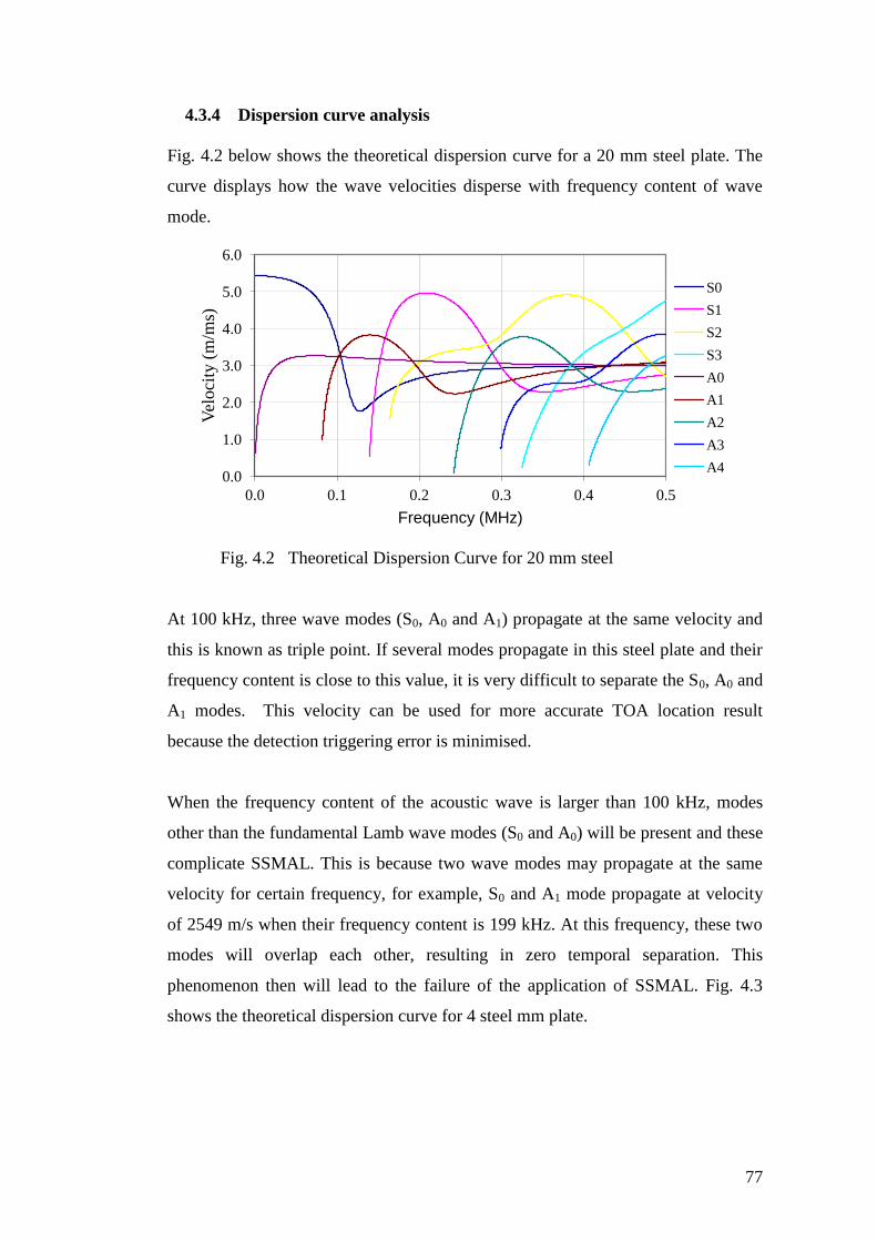
77
4.3.4 Dispersion curve analysis
Fig. 4.2 below shows the theoretical dispersion curve for a 20 mm steel plate. The
curve displays how the wave velocities disperse with frequency content of wave
mode.
Fig. 4.2 Theoretical Dispersion Curve for 20 mm steel
At 100 kHz, three wave modes (S0, A0 and A1) propagate at the same velocity and
this is known as triple point. If several modes propagate in this steel plate and their
frequency content is close to this value, it is very difficult to separate the S0, A0 and
A1 modes. This velocity can be used for more accurate TOA location result
because the detection triggering error is minimised.
When the frequency content of the acoustic wave is larger than 100 kHz, modes
other than the fundamental Lamb wave modes (S0 and A0) will be present and these
complicate SSMAL. This is because two wave modes may propagate at the same
velocity for certain frequency, for example, S0 and A1 mode propagate at velocity
of 2549 m/s when their frequency content is 199 kHz. At this frequency, these two
modes will overlap each other, resulting in zero temporal separation. This
phenomenon then will lead to the failure of the application of SSMAL. Fig. 4.3
shows the theoretical dispersion curve for 4 steel mm plate.
0.0
1.0
2.0
3.0
4.0
5.0
6.0
0.0 0.1 0.2 0.3 0.4 0.5
Vel
oci
ty (
m/m
s)
Frequency (MHz)
S0
S1
S2
S3
A0
A1
A2
A3
A4
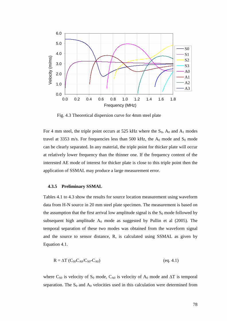
78
Fig. 4.3 Theoretical dispersion curve for 4mm steel plate
For 4 mm steel, the triple point occurs at 525 kHz where the S0, A0 and A1 modes
travel at 3353 m/s. For frequencies less than 500 kHz, the A0 mode and S0 mode
can be clearly separated. In any material, the triple point for thicker plate will occur
at relatively lower frequency than the thinner one. If the frequency content of the
interested AE mode of interest for thicker plate is close to this triple point then the
application of SSMAL may produce a large measurement error.
4.3.5 Preliminary SSMAL
Tables 4.1 to 4.3 show the results for source location measurement using waveform
data from H-N source in 20 mm steel plate specimen. The measurement is based on
the assumption that the first arrival low amplitude signal is the S0 mode followed by
subsequent high amplitude A0 mode as suggested by Pullin et al (2005). The
temporal separation of these two modes was obtained from the waveform signal
and the source to sensor distance, R, is calculated using SSMAL as given by
Equation 4.1.
R = T (CS0CA0/CS0-CA0) (eq. 4.1)
where CS0 is velocity of S0 mode, CA0 is velocity of A0 mode and T is temporal
separation. The S0 and A0 velocities used in this calculation were determined from
0.0
1.0
2.0
3.0
4.0
5.0
6.0
0.0 0.2 0.4 0.6 0.8 1.0 1.2 1.4 1.6 1.8
Ve
locity (
m/m
s)
Frequency (MHz)
S0
S1
S2
S3
A0
A1
A2
A3
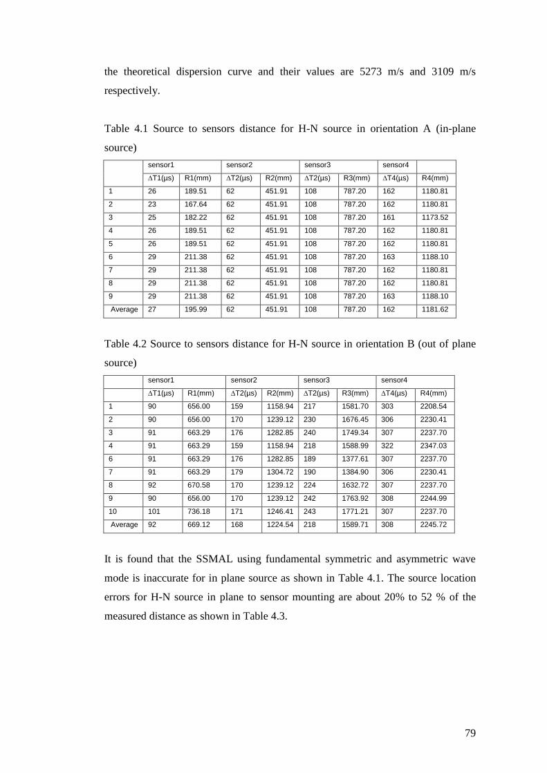
79
the theoretical dispersion curve and their values are 5273 m/s and 3109 m/s
respectively.
Table 4.1 Source to sensors distance for H-N source in orientation A (in-plane
source)
sensor1 sensor2 sensor3 sensor4
∆T1(µs) R1(mm) ∆T2(µs) R2(mm) ∆T2(µs) R3(mm) ∆T4(µs) R4(mm)
1 26 189.51 62 451.91 108 787.20 162 1180.81
2 23 167.64 62 451.91 108 787.20 162 1180.81
3 25 182.22 62 451.91 108 787.20 161 1173.52
4 26 189.51 62 451.91 108 787.20 162 1180.81
5 26 189.51 62 451.91 108 787.20 162 1180.81
6 29 211.38 62 451.91 108 787.20 163 1188.10
7 29 211.38 62 451.91 108 787.20 162 1180.81
8 29 211.38 62 451.91 108 787.20 162 1180.81
9 29 211.38 62 451.91 108 787.20 163 1188.10
Average 27 195.99 62 451.91 108 787.20 162 1181.62
Table 4.2 Source to sensors distance for H-N source in orientation B (out of plane
source)
sensor1 sensor2 sensor3 sensor4
∆T1(µs) R1(mm) ∆T2(µs) R2(mm) ∆T2(µs) R3(mm) ∆T4(µs) R4(mm)
1 90 656.00 159 1158.94 217 1581.70 303 2208.54
2 90 656.00 170 1239.12 230 1676.45 306 2230.41
3 91 663.29 176 1282.85 240 1749.34 307 2237.70
4 91 663.29 159 1158.94 218 1588.99 322 2347.03
6 91 663.29 176 1282.85 189 1377.61 307 2237.70
7 91 663.29 179 1304.72 190 1384.90 306 2230.41
8 92 670.58 170 1239.12 224 1632.72 307 2237.70
9 90 656.00 170 1239.12 242 1763.92 308 2244.99
10 101 736.18 171 1246.41 243 1771.21 307 2237.70
Average 92 669.12 168 1224.54 218 1589.71 308 2245.72
It is found that the SSMAL using fundamental symmetric and asymmetric wave
mode is inaccurate for in plane source as shown in Table 4.1. The source location
errors for H-N source in plane to sensor mounting are about 20% to 52 % of the
measured distance as shown in Table 4.3.
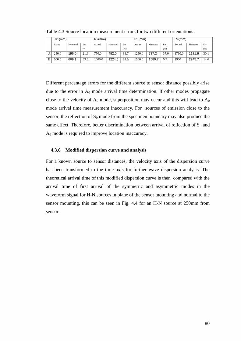
80
Table 4.3 Source location measurement errors for two different orientations.
R1(mm) R2(mm) R3(mm) R4(mm)
Actual Measured Err
(%)
Actual Measured Err
(%)
Act.ual Measured Err
(%)
Act.ual Measured Err
(%)
A 250.0 196.0 21.6 750.0 452.0 39.7 1250.0 787.2 37.0 1710.0 1181.6 30.1
B 500.0 669.1 33.8 1000.0 1224.5 22.5 1500.0 1589.7 5.9 1960 2245.7 14.6
Different percentage errors for the different source to sensor distance possibly arise
due to the error in A0 mode arrival time determination. If other modes propagate
close to the velocity of A0 mode, superposition may occur and this will lead to A0
mode arrival time measurement inaccuracy. For sources of emission close to the
sensor, the reflection of S0 mode from the specimen boundary may also produce the
same effect. Therefore, better discrimination between arrival of reflection of S0 and
A0 mode is required to improve location inaccuracy.
4.3.6 Modified dispersion curve and analysis
For a known source to sensor distances, the velocity axis of the dispersion curve
has been transformed to the time axis for further wave dispersion analysis. The
theoretical arrival time of this modified dispersion curve is then compared with the
arrival time of first arrival of the symmetric and asymmetric modes in the
waveform signal for H-N sources in plane of the sensor mounting and normal to the
sensor mounting, this can be seen in Fig. 4.4 for an H-N source at 250mm from
sensor.
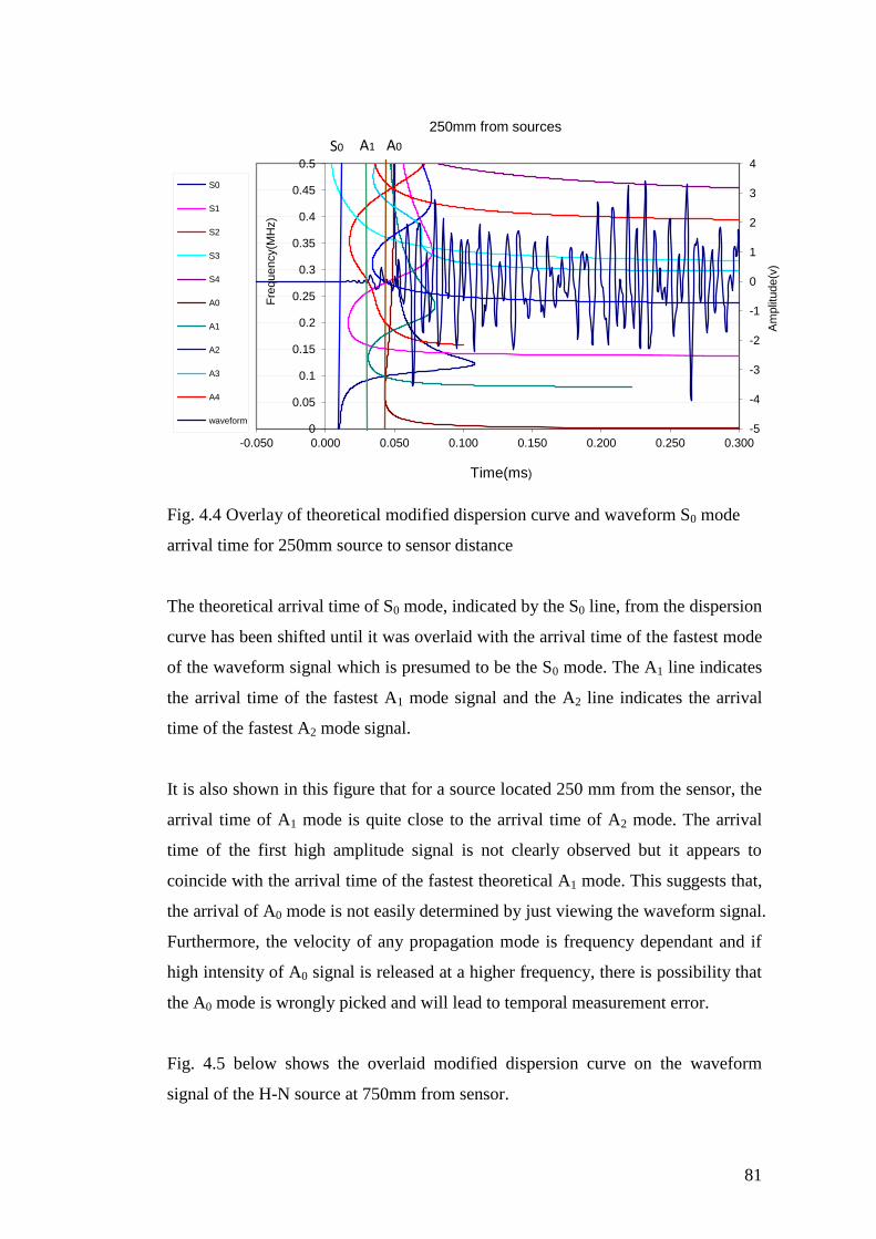
81
Fig. 4.4 Overlay of theoretical modified dispersion curve and waveform S0 mode
arrival time for 250mm source to sensor distance
The theoretical arrival time of S0 mode, indicated by the S0 line, from the dispersion
curve has been shifted until it was overlaid with the arrival time of the fastest mode
of the waveform signal which is presumed to be the S0 mode. The A1 line indicates
the arrival time of the fastest A1 mode signal and the A2 line indicates the arrival
time of the fastest A2 mode signal.
It is also shown in this figure that for a source located 250 mm from the sensor, the
arrival time of A1 mode is quite close to the arrival time of A2 mode. The arrival
time of the first high amplitude signal is not clearly observed but it appears to
coincide with the arrival time of the fastest theoretical A1 mode. This suggests that,
the arrival of A0 mode is not easily determined by just viewing the waveform signal.
Furthermore, the velocity of any propagation mode is frequency dependant and if
high intensity of A0 signal is released at a higher frequency, there is possibility that
the A0 mode is wrongly picked and will lead to temporal measurement error.
Fig. 4.5 below shows the overlaid modified dispersion curve on the waveform
signal of the H-N source at 750mm from sensor.
-5
-4
-3
-2
-1
0
1
2
3
4
0
0.05
0.1
0.15
0.2
0.25
0.3
0.35
0.4
0.45
0.5
-0.050 0.000 0.050 0.100 0.150 0.200 0.250 0.300
Am
plit
ude(v
)
Fre
quency(M
Hz)
Time(ms)
250mm from sources
S0
S1
S2
S3
S4
A0
A1
A2
A3
A4
waveform
S0 A1 A0
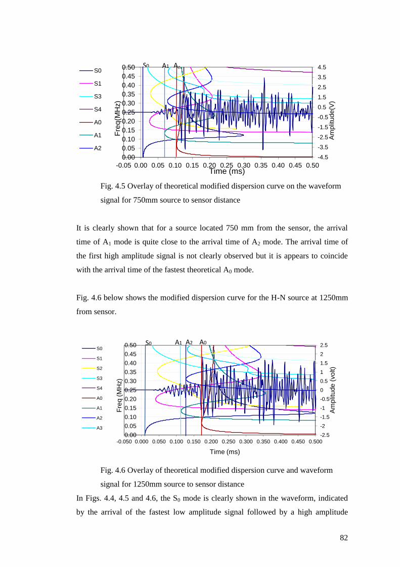
82
Fig. 4.5 Overlay of theoretical modified dispersion curve on the waveform
signal for 750mm source to sensor distance
It is clearly shown that for a source located 750 mm from the sensor, the arrival
time of A1 mode is quite close to the arrival time of A2 mode. The arrival time of
the first high amplitude signal is not clearly observed but it is appears to coincide
with the arrival time of the fastest theoretical A0 mode.
Fig. 4.6 below shows the modified dispersion curve for the H-N source at 1250mm
from sensor.
Fig. 4.6 Overlay of theoretical modified dispersion curve and waveform
signal for 1250mm source to sensor distance
In Figs. 4.4, 4.5 and 4.6, the S0 mode is clearly shown in the waveform, indicated
by the arrival of the fastest low amplitude signal followed by a high amplitude
-4.5
-3.5
-2.5
-1.5
-0.5
0.5
1.5
2.5
3.5
4.5
0.00
0.05
0.10
0.15
0.20
0.25
0.30
0.35
0.40
0.45
0.50
-0.05 0.00 0.05 0.10 0.15 0.20 0.25 0.30 0.35 0.40 0.45 0.50
Am
plit
ude(V
)
Fre
q(M
Hz)
Time (ms)
S0
S1
S3
S4
A0
A1
A2
S0 A1 A0
-2.5
-2
-1.5
-1
-0.5
0
0.5
1
1.5
2
2.5
0.00
0.05
0.10
0.15
0.20
0.25
0.30
0.35
0.40
0.45
0.50
-0.050 0.000 0.050 0.100 0.150 0.200 0.250 0.300 0.350 0.400 0.450 0.500
Am
plit
ude (
volt)
Fre
q (
MH
z)
Time (ms)
S0
S1
S2
S3
S4
A0
A1
A2
A3
S0 A1 A2 A0
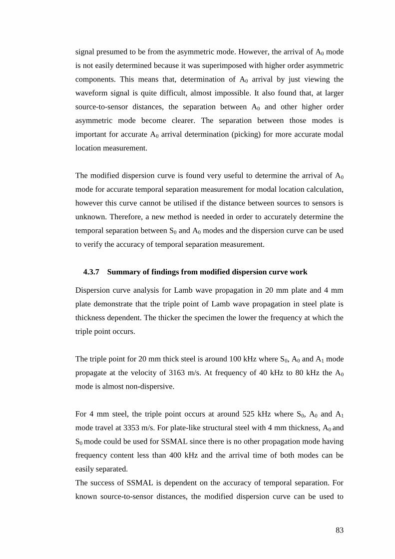
83
signal presumed to be from the asymmetric mode. However, the arrival of A0 mode
is not easily determined because it was superimposed with higher order asymmetric
components. This means that, determination of A0 arrival by just viewing the
waveform signal is quite difficult, almost impossible. It also found that, at larger
source-to-sensor distances, the separation between A0 and other higher order
asymmetric mode become clearer. The separation between those modes is
important for accurate A0 arrival determination (picking) for more accurate modal
location measurement.
The modified dispersion curve is found very useful to determine the arrival of A0
mode for accurate temporal separation measurement for modal location calculation,
however this curve cannot be utilised if the distance between sources to sensors is
unknown. Therefore, a new method is needed in order to accurately determine the
temporal separation between S0 and A0 modes and the dispersion curve can be used
to verify the accuracy of temporal separation measurement.
4.3.7 Summary of findings from modified dispersion curve work
Dispersion curve analysis for Lamb wave propagation in 20 mm plate and 4 mm
plate demonstrate that the triple point of Lamb wave propagation in steel plate is
thickness dependent. The thicker the specimen the lower the frequency at which the
triple point occurs.
The triple point for 20 mm thick steel is around 100 kHz where S0, A0 and A1 mode
propagate at the velocity of 3163 m/s. At frequency of 40 kHz to 80 kHz the A0
mode is almost non-dispersive.
For 4 mm steel, the triple point occurs at around 525 kHz where S0, A0 and A1
mode travel at 3353 m/s. For plate-like structural steel with 4 mm thickness, A0 and
S0 mode could be used for SSMAL since there is no other propagation mode having
frequency content less than 400 kHz and the arrival time of both modes can be
easily separated.
The success of SSMAL is dependent on the accuracy of temporal separation. For
known source-to-sensor distances, the modified dispersion curve can be used to
84
determine the arrival of A0 mode for accurate temporal separation measurement.
However, this curve cannot be utilised if the distance between sources and sensors
is unknown.
The larger the source-to-sensor distances the clearer the separation between A0 and
other higher order symmetric mode. The separation between those modes is
important for accurate A0 arrival determination (picking) for accurate modal
location measurement.
A new method is needed to accurately determine the temporal separation between
S0 and A0 modes and the dispersion curve can be used to verify the accuracy of
temporal separation measurement. If a suitable method is developed for recognising
and picking the first arrival of A0 mode, modal location can be utilised for accurate
thermal fatigue source location and crack size measurement in nuclear piping
system.
The modal location method promises an accurate source location result if the
temporal separation error due to the superposition of A0 mode with other wave
components can be resolved. Temporal separation measurement error in SSMAL
can be improved by deploying time-frequency analysis which can discriminate the
content of the AE signal instead of depending on time domain waveform analysis
for temporal separation measurement.
4.4 Proposed wavelet transform analysis and modal location
(WTML) methodology
4.4.1 Introduction
The wavelet is a very short, time base signal, usually an oscillating signal with one
or several cycles. This wavelet is used as a basis for decomposition of the
waveform into multiple component parts called coefficients, based on location and
scale.
85
WT provides two dimensional coefficients, frequency and time. The strength of
each coefficient provides insight into the percentage of correlation of that particular
wavelet to the waveform. The coefficient value gives a third dimension of the data,
an amplitude or strength associated with them. WT analysis can be divided into two
categories, continuous wavelet transforms and discrete wavelet transforms.
With the wavelet approach, the frequency content and the time localisation of the
waveform signal can be viewed simultaneously. WT analysis can also be used to
discriminate various frequency ranges of AE signals and can be presented in the
time domain signal.
4.4.2 WTML approach
Due to the ability to view the frequency content and the time localisation of the
waveform signal simultaneously, it is proposed that WT can be deployed for more
accurate source location and crack length measurement and improve SSMAL by
providing more accurate temporal separation measurements. WT assisted by a
modified dispersion curve could be used to distinguish the arrival A0 from the
arrival of other components and noise signals. The temporal separation between
those two modes can be accurately measured using wavelet coefficient against time.
This temporal separation measurement can then be utilised in the SSMAL
calculation. WTML source location technique is expected to produce more accurate
source-to-sensor location compared with other location method. The modified
dispersion curve also can be used to validate the WTML location calculation.
This novel approach is called Wavelet Transform analysis and Modal Location
(WTML) method, and it utilises the wavelet coefficient plot against time from WT
analysis to accurately measure the temporal separation between A0 and S0 modes.
In WTML method, temporal separation is measured from first minimum value of
wavelet coefficient of those wavemode components rather than using peak value as
used by other researchers (Jeong 2000, Takemoto 2000, Hamstad 2002, Jinpin 2004,
Alex 2010).
86
It is expected that this temporal separation measurement approach will give more
accurate result since the first minimum wavelet coefficient represents the actual
first arrival wavemode component while the maximum coefficient represents the
peak to peak temporal separation. This temporal separation measurement is then
utilised in the SSMAL calculation and it is expected that WTML approach will
produce more accurate source to sensor location results compared with other
location methods. Furthermore, WTML method utilises the modified dispersion
curve to validate the location calculation accuracy.
The WTML method developed and used in this study involves four main steps;
Waveform acquisition and processing, Source to sensors distance calculation,
Verification of source to sensor distance measurement and Location of events.
1. Waveform acquisition and processing
The AE waveform from AE source is acquired. This waveform is then
transformed into wavelet. This transform will produce the wavelet of the
waveform and the plot of wavelet coefficient strength against time.
2. Source to sensors distance calculation.
The SSMAL equation (Pullin 2005) is used to calculate the source to sensors
distance. However, temporal separation is determined using WT analysis
instead of using the time domain waveform signal. The following are the steps
for source to sensors distance calculation.
a) Calculate theoretical dispersion curve (velocity against frequency) for
material under investigation. The theoretical velocity of fundamental
symmetric (cS0) and asymmetric (cA0) modes from this dispersion
curve need to be determined.
b) Measure the temporal separation between S0 and A0 component from
wavelet coefficient plot for every sensor.
c) Calculate source to sensor distance using the SSMAL equation.
87
3. Verification of source to sensor measurement
This verification is performed by calculating a new dispersion curve,
frequency against time, for material under test using the calculated source
to sensors distance from step 2 a) above. This modified dispersion curve is
then overlaid onto the transformed wavelet from step 1. The position
(time) of S0 and A0 modes is then evaluated against the wavelet, wavelet
coefficient plot and waveform plot.
4. Location of Events.
The circle intersection technique has been used for determining the source
location. For verified source to sensor location from previous step, a circle
is plotted around every sensor and the verified source to sensor distance is
the radius of the circles. The intersection of every circle has been used as
the source location.
4.5 Wavelet Transform Analysis and Modal Location (WTML)
of artificial sources in a steel plate
4.5.1 Experimental setup and validation procedure
MISTRAS WD sensors (working frequency range of 100-1000 kHz) were used
throughout this work. The sensors were mounted on a steel plate and held in
position with magnetic clamps. The plate was manufactured from mild steel with
dimension of 5 mm thick, 790 mm long and 300mm width. Two sharp notches with
length of 50 mm were introduced onto both edges of the specimen as shown in Fig.
4.7 to represent the edge of a crack. Four sensors were mounted onto the plate
surface. A four channel MISTRAS AEwin DiSP data acquisition system was used
for AE waveform acquisition. Detected events were pre-amplified by a 40 dB
preamplifier. The acquired waveforms were stored on the computer for further
analysis.
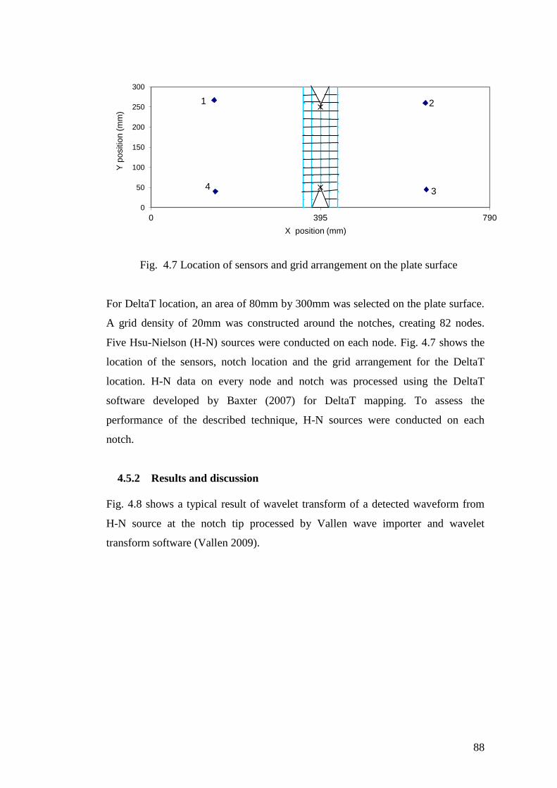
88
Fig. 4.7 Location of sensors and grid arrangement on the plate surface
For DeltaT location, an area of 80mm by 300mm was selected on the plate surface.
A grid density of 20mm was constructed around the notches, creating 82 nodes.
Five Hsu-Nielson (H-N) sources were conducted on each node. Fig. 4.7 shows the
location of the sensors, notch location and the grid arrangement for the DeltaT
location. H-N data on every node and notch was processed using the DeltaT
software developed by Baxter (2007) for DeltaT mapping. To assess the
performance of the described technique, H-N sources were conducted on each
notch.
4.5.2 Results and discussion
Fig. 4.8 shows a typical result of wavelet transform of a detected waveform from
H-N source at the notch tip processed by Vallen wave importer and wavelet
transform software (Vallen 2009).
0
50
100
150
200
250
300
0 395 790
Y p
ositio
n (
mm
)
X position (mm)
1 2
4 3
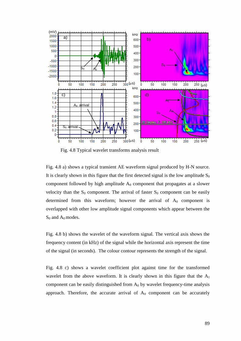
89
Fig. 4.8 Typical wavelet transforms analysis result
Fig. 4.8 a) shows a typical transient AE waveform signal produced by H-N source.
It is clearly shown in this figure that the first detected signal is the low amplitude S0
component followed by high amplitude A0 component that propagates at a slower
velocity than the S0 component. The arrival of faster S0 component can be easily
determined from this waveform; however the arrival of A0 component is
overlapped with other low amplitude signal components which appear between the
S0 and A0 modes.
Fig. 4.8 b) shows the wavelet of the waveform signal. The vertical axis shows the
frequency content (in kHz) of the signal while the horizontal axis represent the time
of the signal (in seconds). The colour contour represents the strength of the signal.
Fig. 4.8 c) shows a wavelet coefficient plot against time for the transformed
wavelet from the above waveform. It is clearly shown in this figure that the A1
component can be easily distinguished from A0 by wavelet frequency-time analysis
approach. Therefore, the accurate arrival of A0 component can be accurately
a) b)
c) d)
S0 A0
(mV) kHz
kHz
)
(s) (s)
(s) (s)
S0
S0 arrival
A0 arrival
A0
A0
S0
A1
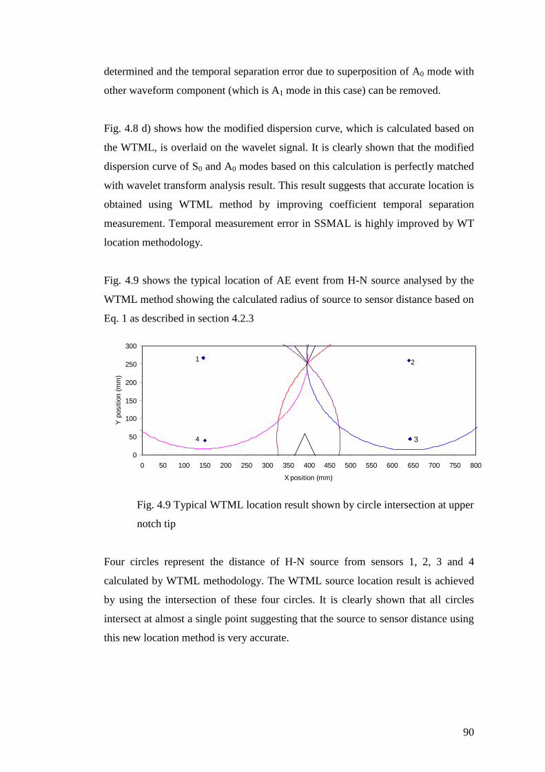
90
determined and the temporal separation error due to superposition of A0 mode with
other waveform component (which is A1 mode in this case) can be removed.
Fig. 4.8 d) shows how the modified dispersion curve, which is calculated based on
the WTML, is overlaid on the wavelet signal. It is clearly shown that the modified
dispersion curve of S0 and A0 modes based on this calculation is perfectly matched
with wavelet transform analysis result. This result suggests that accurate location is
obtained using WTML method by improving coefficient temporal separation
measurement. Temporal measurement error in SSMAL is highly improved by WT
location methodology.
Fig. 4.9 shows the typical location of AE event from H-N source analysed by the
WTML method showing the calculated radius of source to sensor distance based on
Eq. 1 as described in section 4.2.3
Fig. 4.9 Typical WTML location result shown by circle intersection at upper
notch tip
Four circles represent the distance of H-N source from sensors 1, 2, 3 and 4
calculated by WTML methodology. The WTML source location result is achieved
by using the intersection of these four circles. It is clearly shown that all circles
intersect at almost a single point suggesting that the source to sensor distance using
this new location method is very accurate.
0
50
100
150
200
250
300
0 50 100 150 200 250 300 350 400 450 500 550 600 650 700 750 800
X position (mm)
Y p
ositio
n (
mm
)
1 2
4 3
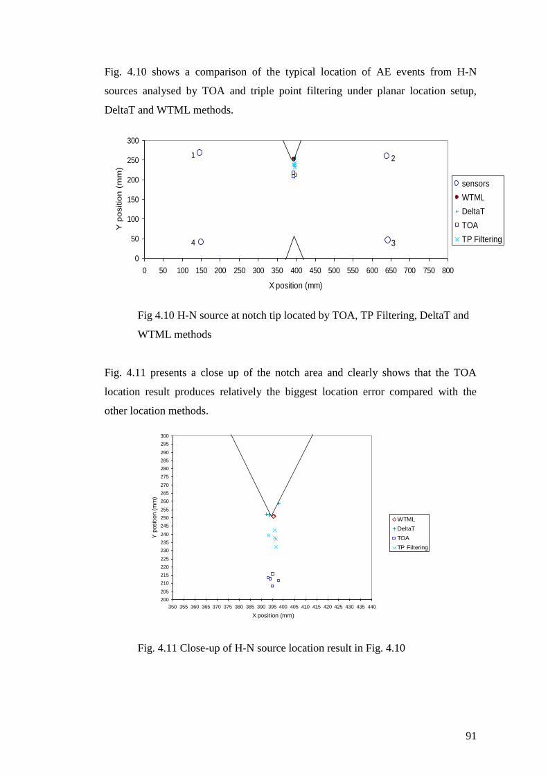
91
Fig. 4.10 shows a comparison of the typical location of AE events from H-N
sources analysed by TOA and triple point filtering under planar location setup,
DeltaT and WTML methods.
Fig 4.10 H-N source at notch tip located by TOA, TP Filtering, DeltaT and
WTML methods
Fig. 4.11 presents a close up of the notch area and clearly shows that the TOA
location result produces relatively the biggest location error compared with the
other location methods.
Fig. 4.11 Close-up of H-N source location result in Fig. 4.10
0
50
100
150
200
250
300
0 50 100 150 200 250 300 350 400 450 500 550 600 650 700 750 800
X position (mm)
Y p
ositio
n (
mm
)
sensors
WTML
DeltaT
TOA
TP Filtering
1 2
4 3
200
205
210
215
220
225
230
235
240
245
250
255
260
265
270
275
280
285
290
295
300
350 355 360 365 370 375 380 385 390 395 400 405 410 415 420 425 430 435 440
X position (mm)
Y p
ositio
n (
mm
)
WTML
DeltaT
TOA
TP Filtering
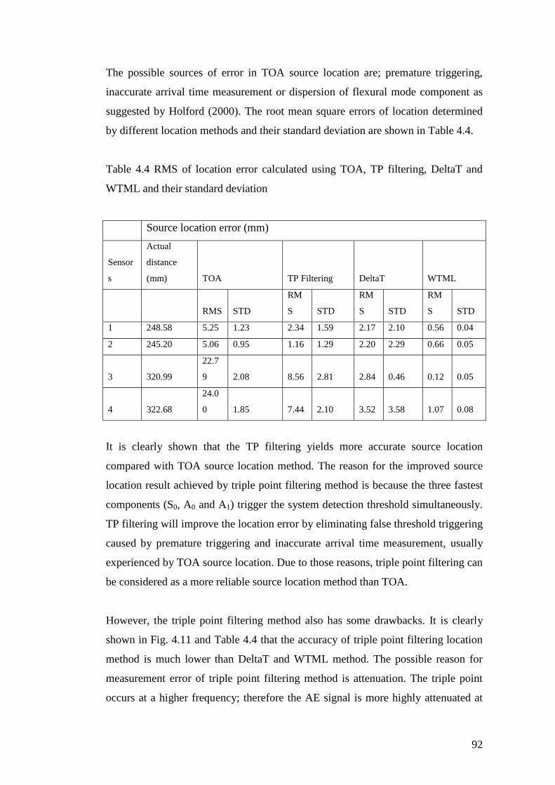
92
The possible sources of error in TOA source location are; premature triggering,
inaccurate arrival time measurement or dispersion of flexural mode component as
suggested by Holford (2000). The root mean square errors of location determined
by different location methods and their standard deviation are shown in Table 4.4.
Table 4.4 RMS of location error calculated using TOA, TP filtering, DeltaT and
WTML and their standard deviation
Source location error (mm)
Sensor
s
Actual
distance
(mm)
TOA
TP Filtering
DeltaT
WTML
RMS STD
RM
S STD
RM
S STD
RM
S STD
1 248.58 5.25 1.23 2.34 1.59 2.17 2.10 0.56 0.04
2 245.20 5.06 0.95 1.16 1.29 2.20 2.29 0.66 0.05
3 320.99
22.7
9 2.08 8.56 2.81 2.84 0.46 0.12 0.05
4 322.68
24.0
0 1.85 7.44 2.10 3.52 3.58 1.07 0.08
It is clearly shown that the TP filtering yields more accurate source location
compared with TOA source location method. The reason for the improved source
location result achieved by triple point filtering method is because the three fastest
components (S0, A0 and A1) trigger the system detection threshold simultaneously.
TP filtering will improve the location error by eliminating false threshold triggering
caused by premature triggering and inaccurate arrival time measurement, usually
experienced by TOA source location. Due to those reasons, triple point filtering can
be considered as a more reliable source location method than TOA.
However, the triple point filtering method also has some drawbacks. It is clearly
shown in Fig. 4.11 and Table 4.4 that the accuracy of triple point filtering location
method is much lower than DeltaT and WTML method. The possible reason for
measurement error of triple point filtering method is attenuation. The triple point
occurs at a higher frequency; therefore the AE signal is more highly attenuated at
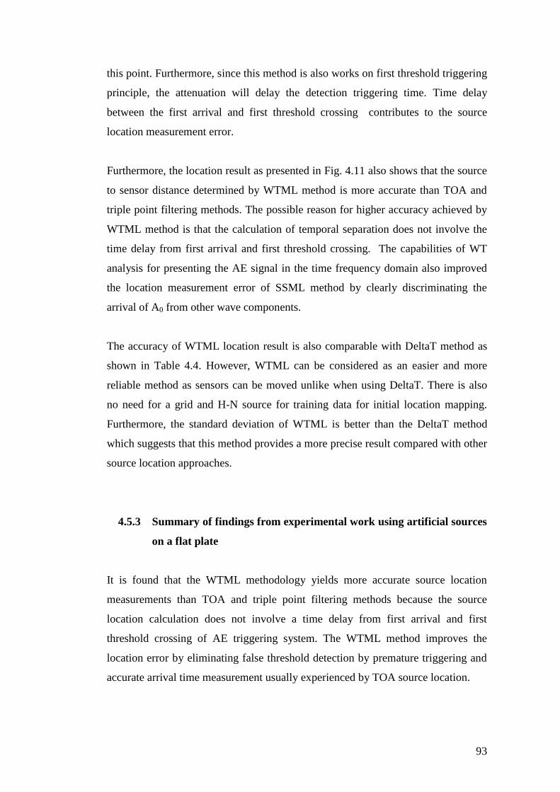
93
this point. Furthermore, since this method is also works on first threshold triggering
principle, the attenuation will delay the detection triggering time. Time delay
between the first arrival and first threshold crossing contributes to the source
location measurement error.
Furthermore, the location result as presented in Fig. 4.11 also shows that the source
to sensor distance determined by WTML method is more accurate than TOA and
triple point filtering methods. The possible reason for higher accuracy achieved by
WTML method is that the calculation of temporal separation does not involve the
time delay from first arrival and first threshold crossing. The capabilities of WT
analysis for presenting the AE signal in the time frequency domain also improved
the location measurement error of SSML method by clearly discriminating the
arrival of A0 from other wave components.
The accuracy of WTML location result is also comparable with DeltaT method as
shown in Table 4.4. However, WTML can be considered as an easier and more
reliable method as sensors can be moved unlike when using DeltaT. There is also
no need for a grid and H-N source for training data for initial location mapping.
Furthermore, the standard deviation of WTML is better than the DeltaT method
which suggests that this method provides a more precise result compared with other
source location approaches.
4.5.3 Summary of findings from experimental work using artificial sources
on a flat plate
It is found that the WTML methodology yields more accurate source location
measurements than TOA and triple point filtering methods because the source
location calculation does not involve a time delay from first arrival and first
threshold crossing of AE triggering system. The WTML method improves the
location error by eliminating false threshold detection by premature triggering and
accurate arrival time measurement usually experienced by TOA source location.
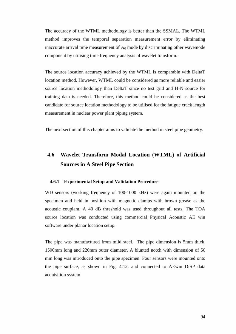
94
The accuracy of the WTML methodology is better than the SSMAL. The WTML
method improves the temporal separation measurement error by eliminating
inaccurate arrival time measurement of A0 mode by discriminating other wavemode
component by utilising time frequency analysis of wavelet transform.
The source location accuracy achieved by the WTML is comparable with DeltaT
location method. However, WTML could be considered as more reliable and easier
source location methodology than DeltaT since no test grid and H-N source for
training data is needed. Therefore, this method could be considered as the best
candidate for source location methodology to be utilised for the fatigue crack length
measurement in nuclear power plant piping system.
The next section of this chapter aims to validate the method in steel pipe geometry.
4.6 Wavelet Transform Modal Location (WTML) of Artificial
Sources in A Steel Pipe Section
4.6.1 Experimental Setup and Validation Procedure
WD sensors (working frequency of 100-1000 kHz) were again mounted on the
specimen and held in position with magnetic clamps with brown grease as the
acoustic couplant. A 40 dB threshold was used throughout all tests. The TOA
source location was conducted using commercial Physical Acoustic AE win
software under planar location setup.
The pipe was manufactured from mild steel. The pipe dimension is 5mm thick,
1500mm long and 220mm outer diameter. A blunted notch with dimension of 50
mm long was introduced onto the pipe specimen. Four sensors were mounted onto
the pipe surface, as shown in Fig. 4.12, and connected to AEwin DiSP data
acquisition system.
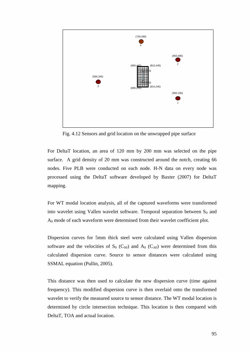
95
Fig. 4.12 Sensors and grid location on the unwrapped pipe surface
For DeltaT location, an area of 120 mm by 200 mm was selected on the pipe
surface. A grid density of 20 mm was constructed around the notch, creating 66
nodes. Five PLB were conducted on each node. H-N data on every node was
processed using the DeltaT software developed by Baxter (2007) for DeltaT
mapping.
For WT modal location analysis, all of the captured waveforms were transformed
into wavelet using Vallen wavelet software. Temporal separation between S0 and
A0 mode of each waveform were determined from their wavelet coefficient plot.
Dispersion curves for 5mm thick steel were calculated using Vallen dispersion
software and the velocities of S0 (CS0) and A0 (CA0) were determined from this
calculated dispersion curve. Source to sensor distances were calculated using
SSMAL equation (Pullin, 2005).
This distance was then used to calculate the new dispersion curve (time against
frequency). This modified dispersion curve is then overlaid onto the transformed
wavelet to verify the measured source to sensor distance. The WT modal location is
determined by circle intersection technique. This location is then compared with
DeltaT, TOA and actual location.
1
2
3
4
(750,590)
(950,495)
(950,195)
(590,345)
(810,445)
(810,245)
(690,445)
(690,245)
(750,320)
(750,370)
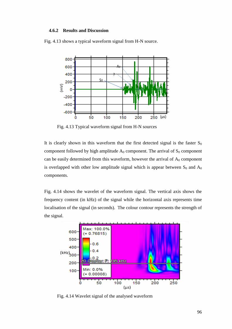
96
4.6.2 Results and Discussion
Fig. 4.13 shows a typical waveform signal from H-N source.
Fig. 4.13 Typical waveform signal from H-N sources
It is clearly shown in this waveform that the first detected signal is the faster S0
component followed by high amplitude A0 component. The arrival of S0 component
can be easily determined from this waveform, however the arrival of A0 component
is overlapped with other low amplitude signal which is appear between S0 and A0
components.
Fig. 4.14 shows the wavelet of the waveform signal. The vertical axis shows the
frequency content (in kHz) of the signal while the horizontal axis represents time
localisation of the signal (in seconds). The colour contour represents the strength of
the signal.
Fig. 4.14 Wavelet signal of the analysed waveform
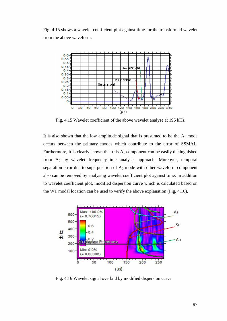
97
Fig. 4.15 shows a wavelet coefficient plot against time for the transformed wavelet
from the above waveform.
Fig. 4.15 Wavelet coefficient of the above wavelet analyse at 195 kHz
It is also shown that the low amplitude signal that is presumed to be the A1 mode
occurs between the primary modes which contribute to the error of SSMAL.
Furthermore, it is clearly shown that this A1 component can be easily distinguished
from A0 by wavelet frequency-time analysis approach. Moreover, temporal
separation error due to superposition of A0 mode with other waveform component
also can be removed by analysing wavelet coefficient plot against time. In addition
to wavelet coefficient plot, modified dispersion curve which is calculated based on
the WT modal location can be used to verify the above explanation (Fig. 4.16).
Fig. 4.16 Wavelet signal overlaid by modified dispersion curve
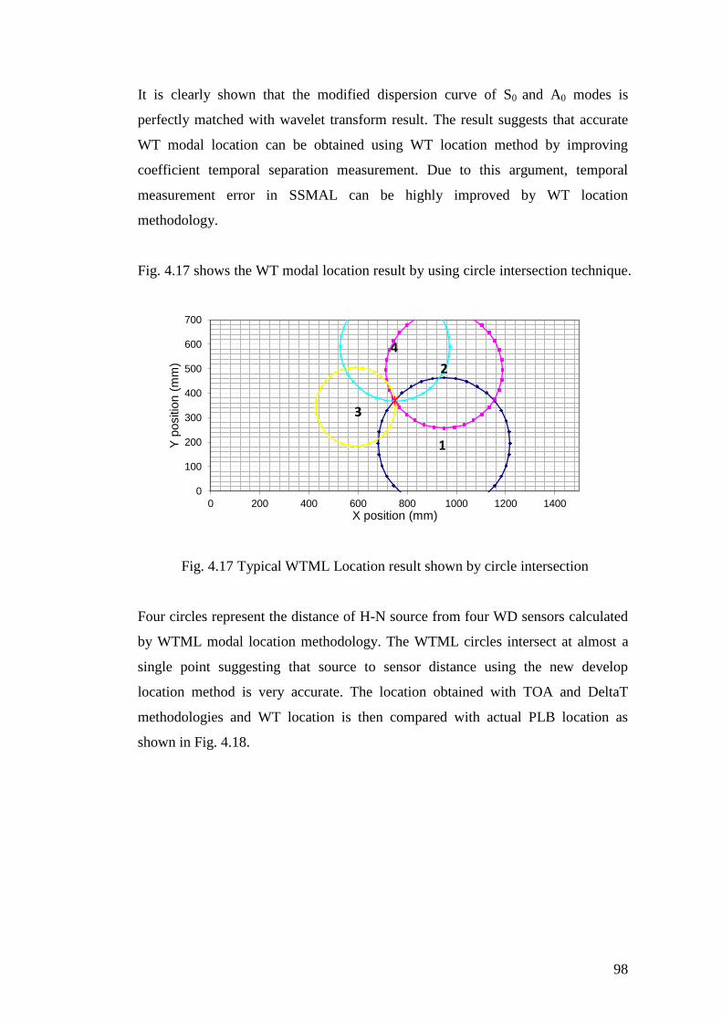
98
It is clearly shown that the modified dispersion curve of S0 and A0 modes is
perfectly matched with wavelet transform result. The result suggests that accurate
WT modal location can be obtained using WT location method by improving
coefficient temporal separation measurement. Due to this argument, temporal
measurement error in SSMAL can be highly improved by WT location
methodology.
Fig. 4.17 shows the WT modal location result by using circle intersection technique.
Fig. 4.17 Typical WTML Location result shown by circle intersection
Four circles represent the distance of H-N source from four WD sensors calculated
by WTML modal location methodology. The WTML circles intersect at almost a
single point suggesting that source to sensor distance using the new develop
location method is very accurate. The location obtained with TOA and DeltaT
methodologies and WT location is then compared with actual PLB location as
shown in Fig. 4.18.
0
100
200
300
400
500
600
700
0 200 400 600 800 1000 1200 1400
Y p
ositio
n (
mm
)
X position (mm)
1
2
3
4
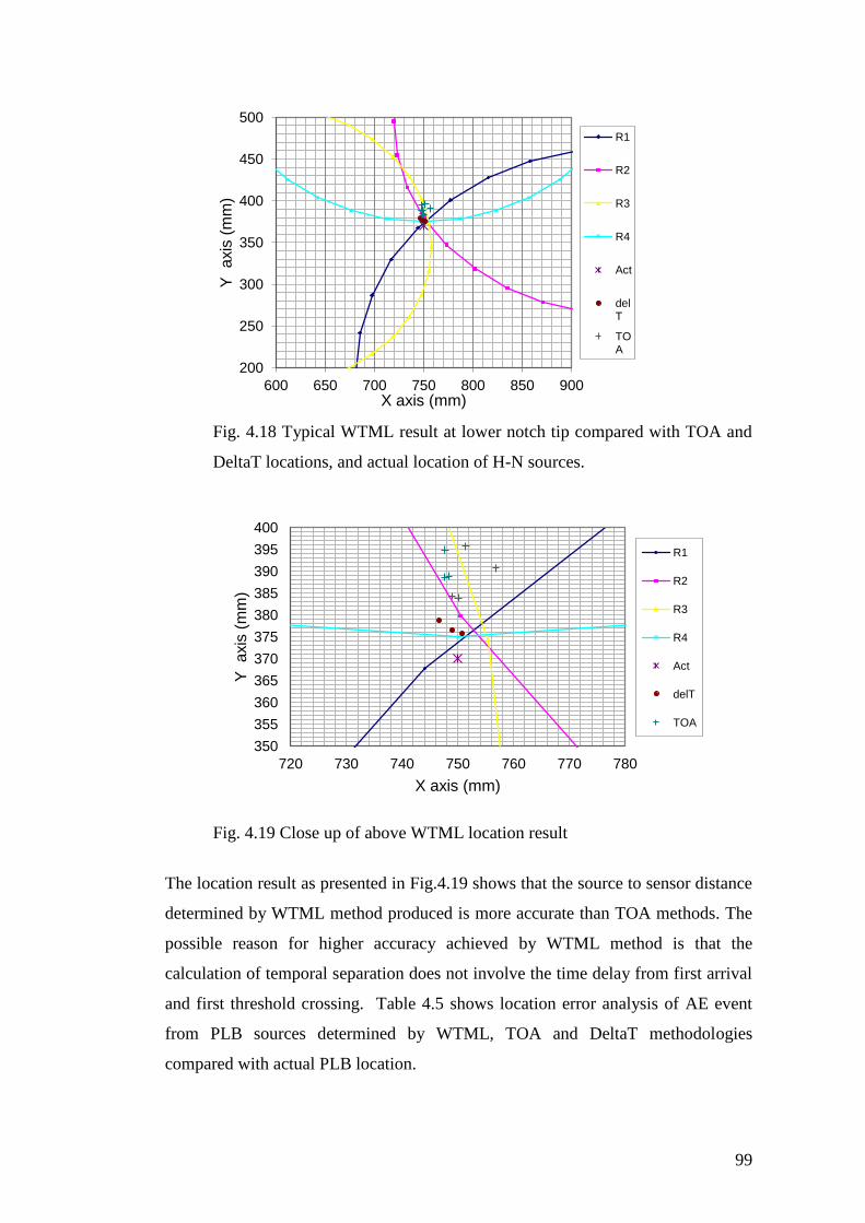
99
Fig. 4.18 Typical WTML result at lower notch tip compared with TOA and
DeltaT locations, and actual location of H-N sources.
Fig. 4.19 Close up of above WTML location result
The location result as presented in Fig.4.19 shows that the source to sensor distance
determined by WTML method produced is more accurate than TOA methods. The
possible reason for higher accuracy achieved by WTML method is that the
calculation of temporal separation does not involve the time delay from first arrival
and first threshold crossing. Table 4.5 shows location error analysis of AE event
from PLB sources determined by WTML, TOA and DeltaT methodologies
compared with actual PLB location.
200
250
300
350
400
450
500
600 650 700 750 800 850 900
Y a
xis
(m
m)
X axis (mm)
R1
R2
R3
R4
Act
delT
TOA
350
355
360
365
370
375
380
385
390
395
400
720 730 740 750 760 770 780
Y a
xis
(m
m)
X axis (mm)
R1
R2
R3
R4
Act
delT
TOA
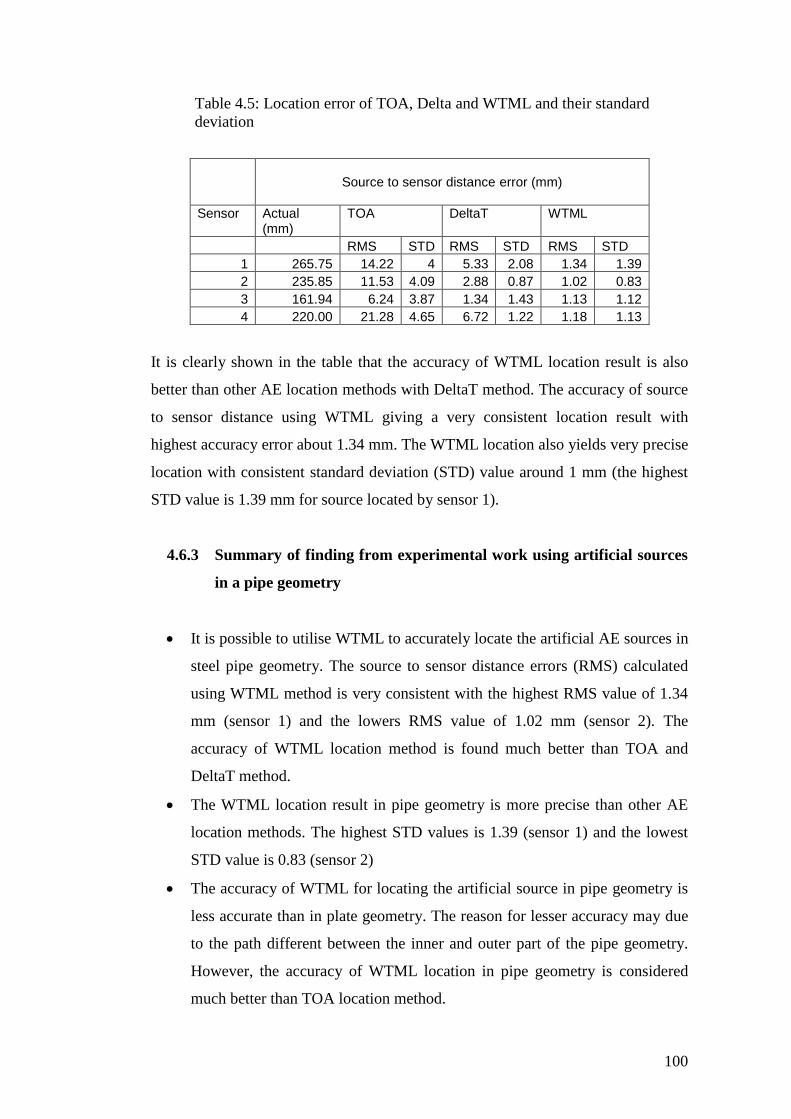
100
Table 4.5: Location error of TOA, Delta and WTML and their standard
deviation
Source to sensor distance error (mm)
Sensor
Actual (mm)
TOA
DeltaT
WTML
RMS STD RMS STD RMS STD
1 265.75 14.22 4 5.33 2.08 1.34 1.39
2 235.85 11.53 4.09 2.88 0.87 1.02 0.83
3 161.94 6.24 3.87 1.34 1.43 1.13 1.12
4 220.00 21.28 4.65 6.72 1.22 1.18 1.13
It is clearly shown in the table that the accuracy of WTML location result is also
better than other AE location methods with DeltaT method. The accuracy of source
to sensor distance using WTML giving a very consistent location result with
highest accuracy error about 1.34 mm. The WTML location also yields very precise
location with consistent standard deviation (STD) value around 1 mm (the highest
STD value is 1.39 mm for source located by sensor 1).
4.6.3 Summary of finding from experimental work using artificial sources
in a pipe geometry
It is possible to utilise WTML to accurately locate the artificial AE sources in
steel pipe geometry. The source to sensor distance errors (RMS) calculated
using WTML method is very consistent with the highest RMS value of 1.34
mm (sensor 1) and the lowers RMS value of 1.02 mm (sensor 2). The
accuracy of WTML location method is found much better than TOA and
DeltaT method.
The WTML location result in pipe geometry is more precise than other AE
location methods. The highest STD values is 1.39 (sensor 1) and the lowest
STD value is 0.83 (sensor 2)
The accuracy of WTML for locating the artificial source in pipe geometry is
less accurate than in plate geometry. The reason for lesser accuracy may due
to the path different between the inner and outer part of the pipe geometry.
However, the accuracy of WTML location in pipe geometry is considered
much better than TOA location method.
101
4.7 Conclusions and future work
• WTML method was successfully developed for more accurate AE source
location in this study.
• WTML methodology produced more accurate source location than TOA
since calculation does not involve time delay from first arrival and first
threshold crossing
• WTML methodology produced more accurate source location than SSMAL
since the temporal separation can be more accurately measured
• WTML produced more reliable and easier source location methodology
than DeltaT since a grid and H-N source for training data is not required
• This method could be considered as the best candidate for source location
methodology to be utilised for the fatigue crack length measurement in
nuclear power plant piping system
• Further work aims to validate the workability of this method for detection of
actual crack growth in cracked plate and pipe
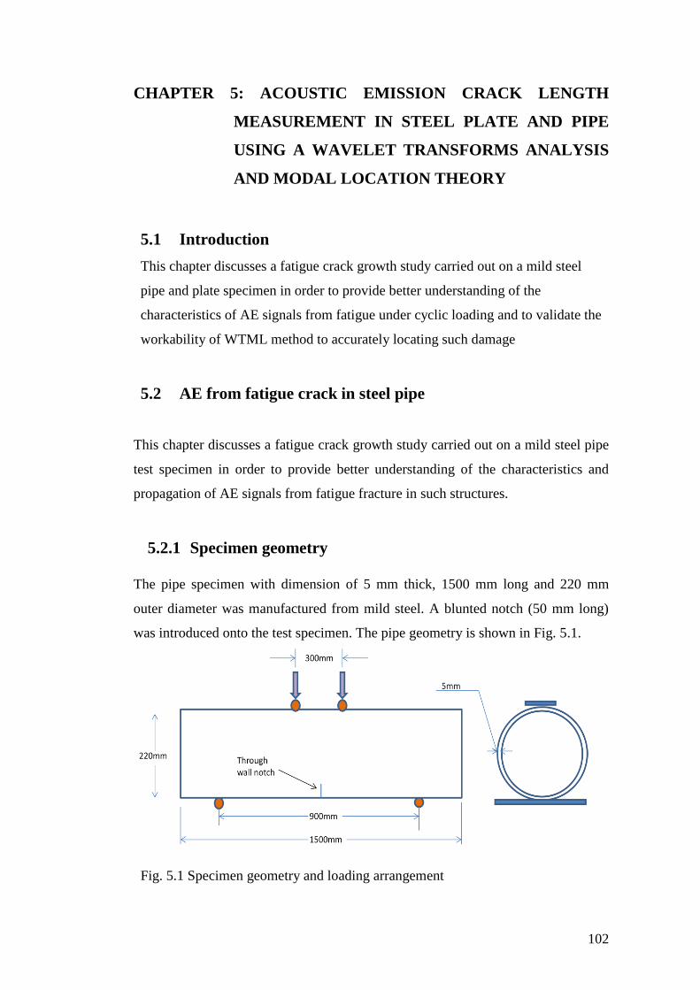
102
CHAPTER 5: ACOUSTIC EMISSION CRACK LENGTH
MEASUREMENT IN STEEL PLATE AND PIPE
USING A WAVELET TRANSFORMS ANALYSIS
AND MODAL LOCATION THEORY
5.1 Introduction
This chapter discusses a fatigue crack growth study carried out on a mild steel
pipe and plate specimen in order to provide better understanding of the
characteristics of AE signals from fatigue under cyclic loading and to validate the
workability of WTML method to accurately locating such damage
5.2 AE from fatigue crack in steel pipe
This chapter discusses a fatigue crack growth study carried out on a mild steel pipe
test specimen in order to provide better understanding of the characteristics and
propagation of AE signals from fatigue fracture in such structures.
5.2.1 Specimen geometry
The pipe specimen with dimension of 5 mm thick, 1500 mm long and 220 mm
outer diameter was manufactured from mild steel. A blunted notch (50 mm long)
was introduced onto the test specimen. The pipe geometry is shown in Fig. 5.1.
Fig. 5.1 Specimen geometry and loading arrangement
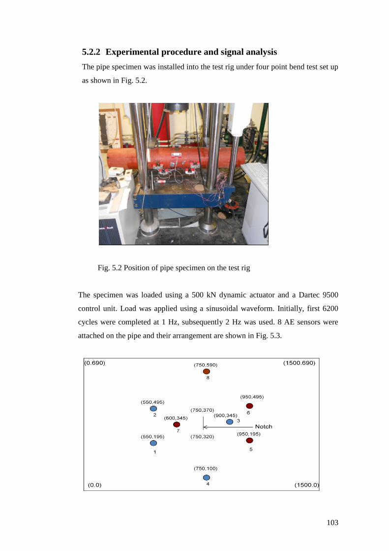
103
5.2.2 Experimental procedure and signal analysis
The pipe specimen was installed into the test rig under four point bend test set up
as shown in Fig. 5.2.
Fig. 5.2 Position of pipe specimen on the test rig
The specimen was loaded using a 500 kN dynamic actuator and a Dartec 9500
control unit. Load was applied using a sinusoidal waveform. Initially, first 6200
cycles were completed at 1 Hz, subsequently 2 Hz was used. 8 AE sensors were
attached on the pipe and their arrangement are shown in Fig. 5.3.
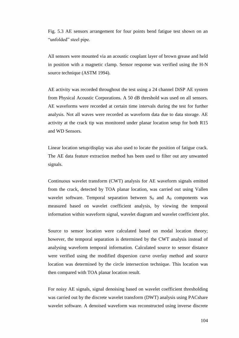
104
Fig. 5.3 AE sensors arrangement for four points bend fatigue test shown on an
“unfolded” steel pipe.
All sensors were mounted via an acoustic couplant layer of brown grease and held
in position with a magnetic clamp. Sensor response was verified using the H-N
source technique (ASTM 1994).
AE activity was recorded throughout the test using a 24 channel DiSP AE system
from Physical Acoustic Corporations. A 50 dB threshold was used on all sensors.
AE waveforms were recorded at certain time intervals during the test for further
analysis. Not all waves were recorded as waveform data due to data storage. AE
activity at the crack tip was monitored under planar location setup for both R15
and WD Sensors.
Linear location setup/display was also used to locate the position of fatigue crack.
The AE data feature extraction method has been used to filter out any unwanted
signals.
Continuous wavelet transform (CWT) analysis for AE waveform signals emitted
from the crack, detected by TOA planar location, was carried out using Vallen
wavelet software. Temporal separation between S0 and A0 components was
measured based on wavelet coefficient analysis, by viewing the temporal
information within waveform signal, wavelet diagram and wavelet coefficient plot.
Source to sensor location were calculated based on modal location theory;
however, the temporal separation is determined by the CWT analysis instead of
analysing waveform temporal information. Calculated source to sensor distance
were verified using the modified dispersion curve overlay method and source
location was determined by the circle intersection technique. This location was
then compared with TOA planar location result.
For noisy AE signals, signal denoising based on wavelet coefficient thresholding
was carried out by the discrete wavelet transform (DWT) analysis using PACshare
wavelet software. A denoised waveform was reconstructed using inverse discrete
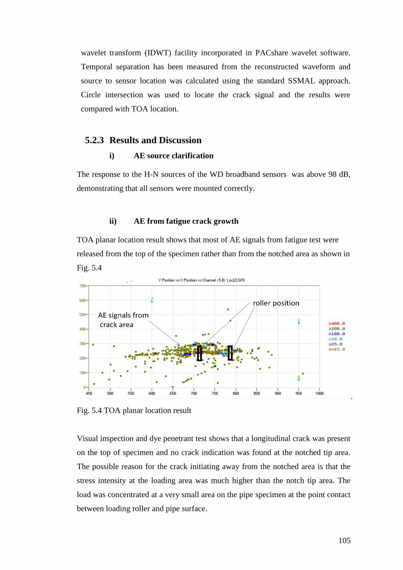
105
wavelet transform (IDWT) facility incorporated in PACshare wavelet software.
Temporal separation has been measured from the reconstructed waveform and
source to sensor location was calculated using the standard SSMAL approach.
Circle intersection was used to locate the crack signal and the results were
compared with TOA location.
5.2.3 Results and Discussion
i) AE source clarification
The response to the H-N sources of the WD broadband sensors was above 98 dB,
demonstrating that all sensors were mounted correctly.
ii) AE from fatigue crack growth
TOA planar location result shows that most of AE signals from fatigue test were
released from the top of the specimen rather than from the notched area as shown in
Fig. 5.4
.
Fig. 5.4 TOA planar location result
Visual inspection and dye penetrant test shows that a longitudinal crack was present
on the top of specimen and no crack indication was found at the notched tip area.
The possible reason for the crack initiating away from the notched area is that the
stress intensity at the loading area was much higher than the notch tip area. The
load was concentrated at a very small area on the pipe specimen at the point contact
between loading roller and pipe surface.
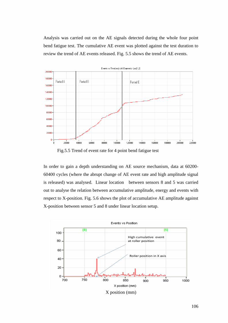
106
Analysis was carried out on the AE signals detected during the whole four point
bend fatigue test. The cumulative AE event was plotted against the test duration to
review the trend of AE events released. Fig. 5.5 shows the trend of AE events.
Fig.5.5 Trend of event rate for 4 point bend fatigue test
In order to gain a depth understanding on AE source mechanism, data at 60200-
60400 cycles (where the abrupt change of AE event rate and high amplitude signal
is released) was analysed. Linear location between sensors 8 and 5 was carried
out to analyse the relation between accumulative amplitude, energy and events with
respect to X-position. Fig. 5.6 shows the plot of accumulative AE amplitude against
X-position between sensor 5 and 8 under linear location setup.
X position (mm)
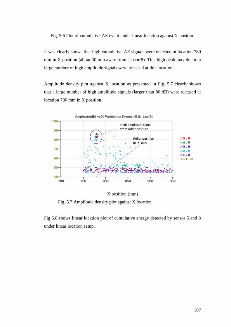
107
Fig. 5.6 Plot of cumulative AE event under linear location against X-position
It was clearly shows that high cumulative AE signals were detected at location 780
mm in X position (about 30 mm away from sensor 8). This high peak may due to a
large number of high amplitude signals were released at this location.
Amplitude density plot against X location as presented in Fig. 5.7 clearly shows
that a large number of high amplitude signals (larger than 80 dB) were released at
location 780 mm in X position.
X position (mm)
Fig. 5.7 Amplitude density plot against X location
Fig 5.8 shows linear location plot of cumulative energy detected by sensor 5 and 8
under linear location setup.
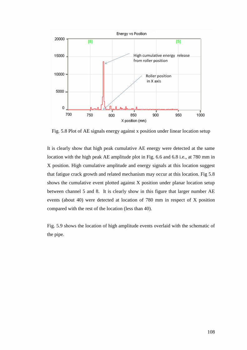
108
Fig. 5.8 Plot of AE signals energy against x position under linear location setup
It is clearly show that high peak cumulative AE energy were detected at the same
location with the high peak AE amplitude plot in Fig. 6.6 and 6.8 i.e., at 780 mm in
X position. High cumulative amplitude and energy signals at this location suggest
that fatigue crack growth and related mechanism may occur at this location. Fig 5.8
shows the cumulative event plotted against X position under planar location setup
between channel 5 and 8. It is clearly show in this figure that larger number AE
events (about 40) were detected at location of 780 mm in respect of X position
compared with the rest of the location (less than 40).
Fig. 5.9 shows the location of high amplitude events overlaid with the schematic of
the pipe.
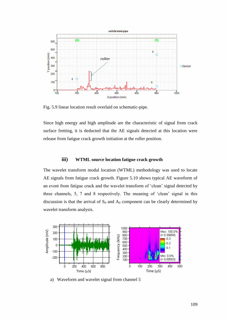
109
Fig. 5.9 linear location result overlaid on schematic-pipe.
Since high energy and high amplitude are the characteristic of signal from crack
surface fretting, it is deducted that the AE signals detected at this location were
release from fatigue crack growth initiation at the roller position.
iii) WTML source location fatigue crack growth
The wavelet transform modal location (WTML) methodology was used to locate
AE signals from fatigue crack growth. Figure 5.10 shows typical AE waveform of
an event from fatigue crack and the wavelet transform of ‘clean’ signal detected by
three channels, 5, 7 and 8 respectively. The meaning of ‘clean’ signal in this
discussion is that the arrival of S0 and A0 component can be clearly determined by
wavelet transform analysis.
a) Waveform and wavelet signal from channel 5
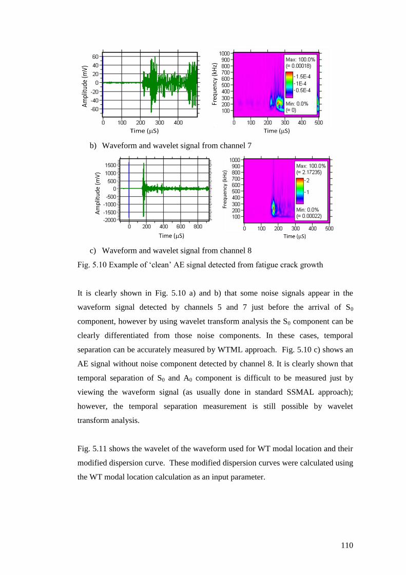
110
b) Waveform and wavelet signal from channel 7
c) Waveform and wavelet signal from channel 8
Fig. 5.10 Example of ‘clean’ AE signal detected from fatigue crack growth
It is clearly shown in Fig. 5.10 a) and b) that some noise signals appear in the
waveform signal detected by channels 5 and 7 just before the arrival of S0
component, however by using wavelet transform analysis the S0 component can be
clearly differentiated from those noise components. In these cases, temporal
separation can be accurately measured by WTML approach. Fig. 5.10 c) shows an
AE signal without noise component detected by channel 8. It is clearly shown that
temporal separation of S0 and A0 component is difficult to be measured just by
viewing the waveform signal (as usually done in standard SSMAL approach);
however, the temporal separation measurement is still possible by wavelet
transform analysis.
Fig. 5.11 shows the wavelet of the waveform used for WT modal location and their
modified dispersion curve. These modified dispersion curves were calculated using
the WT modal location calculation as an input parameter.
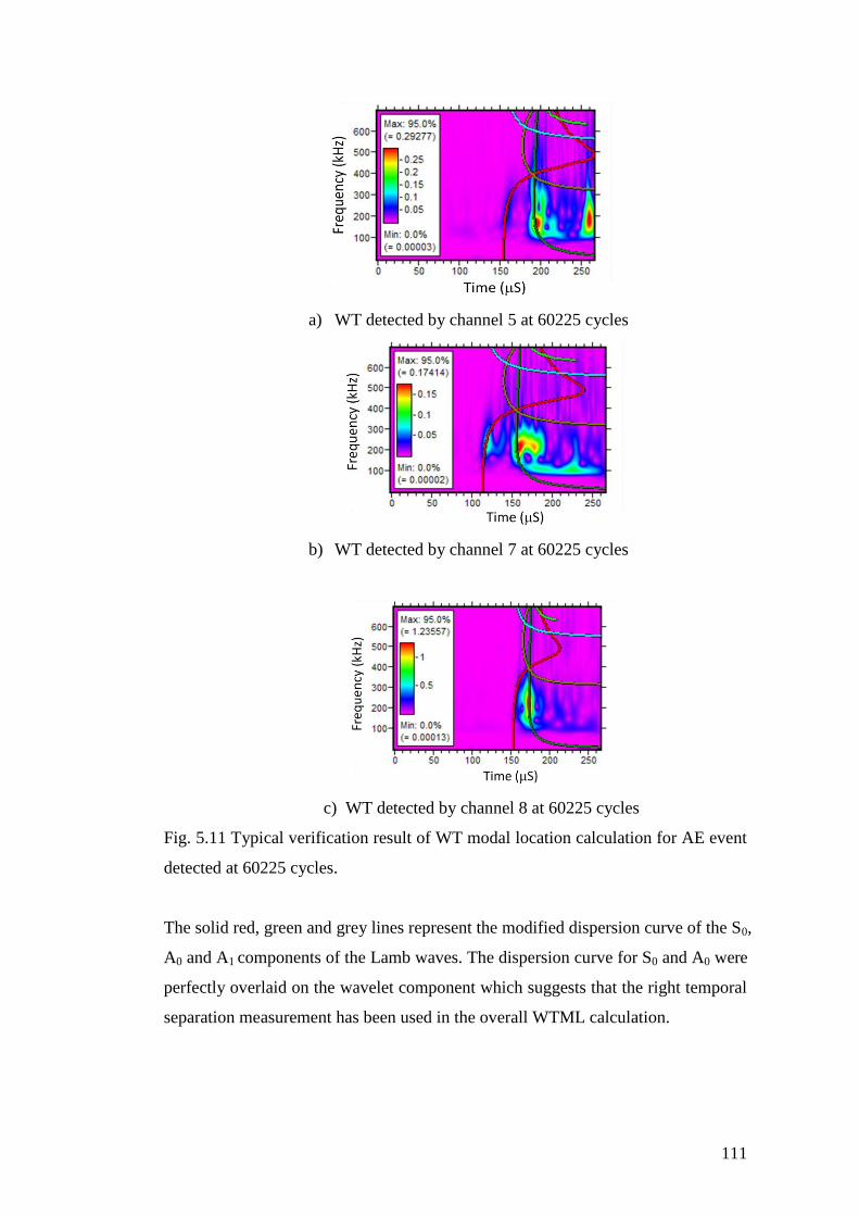
111
a) WT detected by channel 5 at 60225 cycles
b) WT detected by channel 7 at 60225 cycles
c) WT detected by channel 8 at 60225 cycles
Fig. 5.11 Typical verification result of WT modal location calculation for AE event
detected at 60225 cycles.
The solid red, green and grey lines represent the modified dispersion curve of the S0,
A0 and A1 components of the Lamb waves. The dispersion curve for S0 and A0 were
perfectly overlaid on the wavelet component which suggests that the right temporal
separation measurement has been used in the overall WTML calculation.
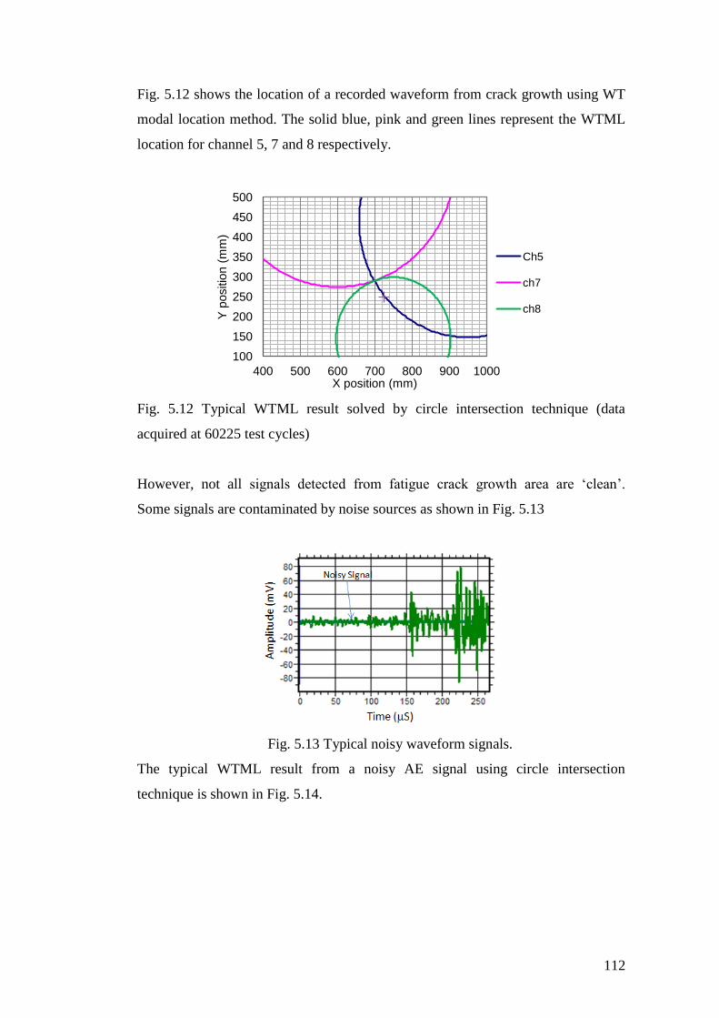
112
Fig. 5.12 shows the location of a recorded waveform from crack growth using WT
modal location method. The solid blue, pink and green lines represent the WTML
location for channel 5, 7 and 8 respectively.
Fig. 5.12 Typical WTML result solved by circle intersection technique (data
acquired at 60225 test cycles)
However, not all signals detected from fatigue crack growth area are ‘clean’.
Some signals are contaminated by noise sources as shown in Fig. 5.13
Fig. 5.13 Typical noisy waveform signals.
The typical WTML result from a noisy AE signal using circle intersection
technique is shown in Fig. 5.14.
100
150
200
250
300
350
400
450
500
400 500 600 700 800 900 1000
Y p
ositio
n (
mm
)
X position (mm)
Ch5
ch7
ch8
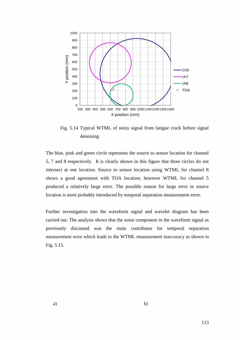
113
Fig. 5.14 Typical WTML of noisy signal from fatigue crack before signal
denoising
The blue, pink and green circle represents the source to sensor location for channel
5, 7 and 8 respectively. It is clearly shown in this figure that three circles do not
intersect at one location. Source to sensor location using WTML for channel 8
shows a good agreement with TOA location; however WTML for channel 5
produced a relatively large error. The possible reason for large error in source
location is most probably introduced by temporal separation measurement error.
Further investigation into the waveform signal and wavelet diagram has been
carried out. The analysis shows that the noise component in the waveform signal as
previously discussed was the main contributor for temporal separation
measurement error which leads to the WTML measurement inaccuracy as shown in
Fig. 5.15.
a) b)
0
100
200
300
400
500
600
700
800
900
1000
200 300 400 500 600 700 800 900 1000 1100 1200 1300 1400
Y p
ositio
n (
mm
)
X position (mm)
Ch5
ch7
ch8
TOA
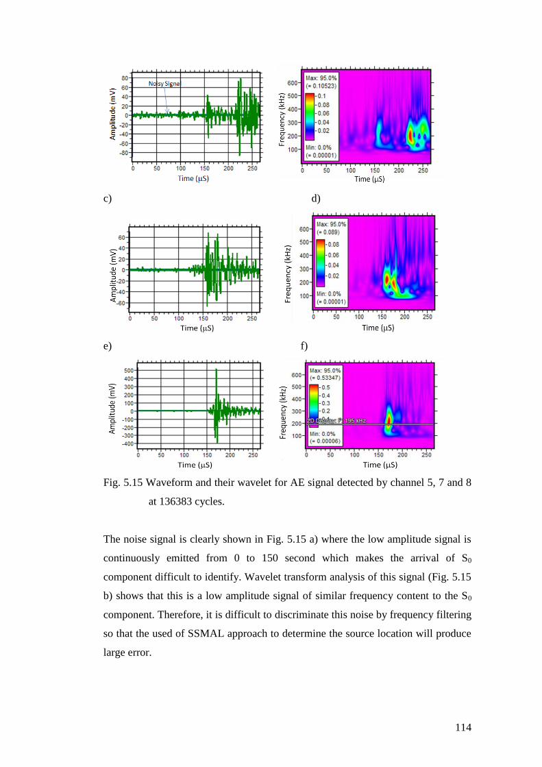
114
c) d)
e) f)
Fig. 5.15 Waveform and their wavelet for AE signal detected by channel 5, 7 and 8
at 136383 cycles.
The noise signal is clearly shown in Fig. 5.15 a) where the low amplitude signal is
continuously emitted from 0 to 150 second which makes the arrival of S0
component difficult to identify. Wavelet transform analysis of this signal (Fig. 5.15
b) shows that this is a low amplitude signal of similar frequency content to the S0
component. Therefore, it is difficult to discriminate this noise by frequency filtering
so that the used of SSMAL approach to determine the source location will produce
large error.
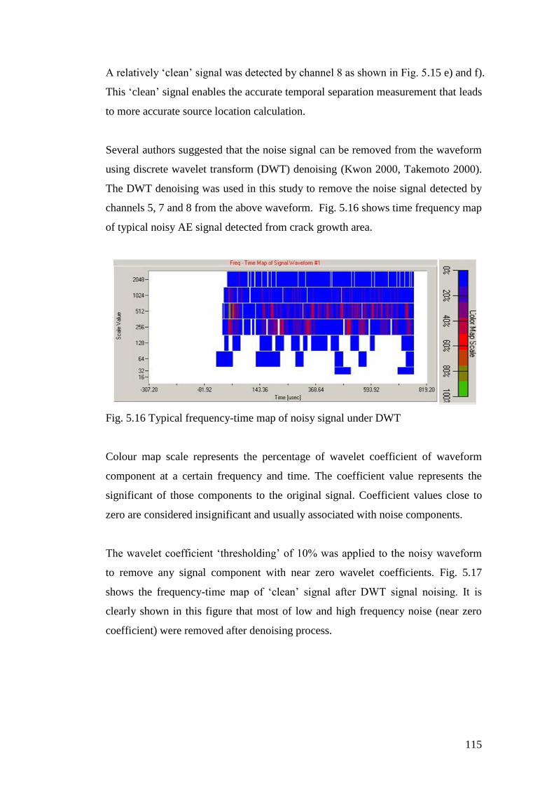
115
A relatively ‘clean’ signal was detected by channel 8 as shown in Fig. 5.15 e) and f).
This ‘clean’ signal enables the accurate temporal separation measurement that leads
to more accurate source location calculation.
Several authors suggested that the noise signal can be removed from the waveform
using discrete wavelet transform (DWT) denoising (Kwon 2000, Takemoto 2000).
The DWT denoising was used in this study to remove the noise signal detected by
channels 5, 7 and 8 from the above waveform. Fig. 5.16 shows time frequency map
of typical noisy AE signal detected from crack growth area.
Fig. 5.16 Typical frequency-time map of noisy signal under DWT
Colour map scale represents the percentage of wavelet coefficient of waveform
component at a certain frequency and time. The coefficient value represents the
significant of those components to the original signal. Coefficient values close to
zero are considered insignificant and usually associated with noise components.
The wavelet coefficient ‘thresholding’ of 10% was applied to the noisy waveform
to remove any signal component with near zero wavelet coefficients. Fig. 5.17
shows the frequency-time map of ‘clean’ signal after DWT signal noising. It is
clearly shown in this figure that most of low and high frequency noise (near zero
coefficient) were removed after denoising process.
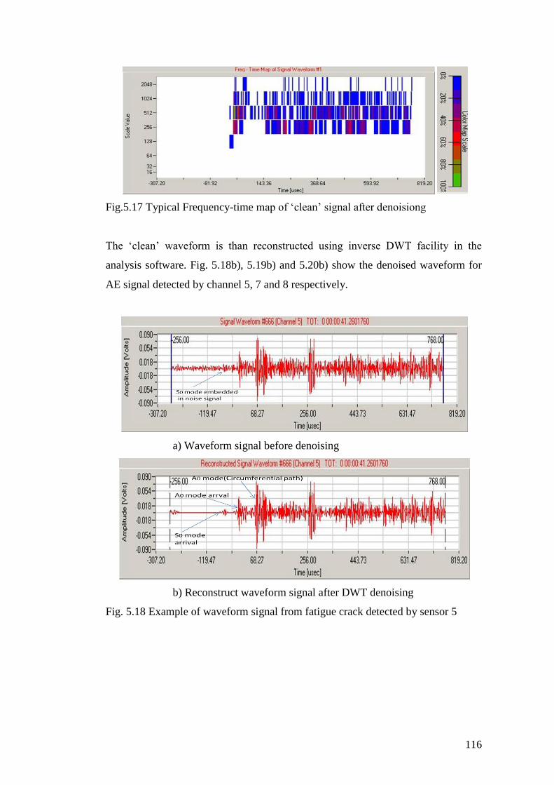
116
Fig.5.17 Typical Frequency-time map of ‘clean’ signal after denoisiong
The ‘clean’ waveform is than reconstructed using inverse DWT facility in the
analysis software. Fig. 5.18b), 5.19b) and 5.20b) show the denoised waveform for
AE signal detected by channel 5, 7 and 8 respectively.
a) Waveform signal before denoising
b) Reconstruct waveform signal after DWT denoising
Fig. 5.18 Example of waveform signal from fatigue crack detected by sensor 5
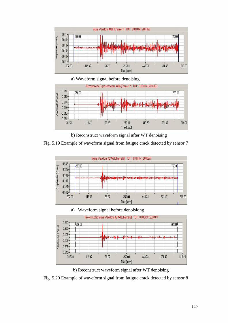
117
a) Waveform signal before denoising
b) Reconstruct waveform signal after WT denoising
Fig. 5.19 Example of waveform signal from fatigue crack detected by sensor 7
a) Waveform signal before denoisiong
b) Reconstruct waveform signal after WT denoising
Fig. 5.20 Example of waveform signal from fatigue crack detected by sensor 8
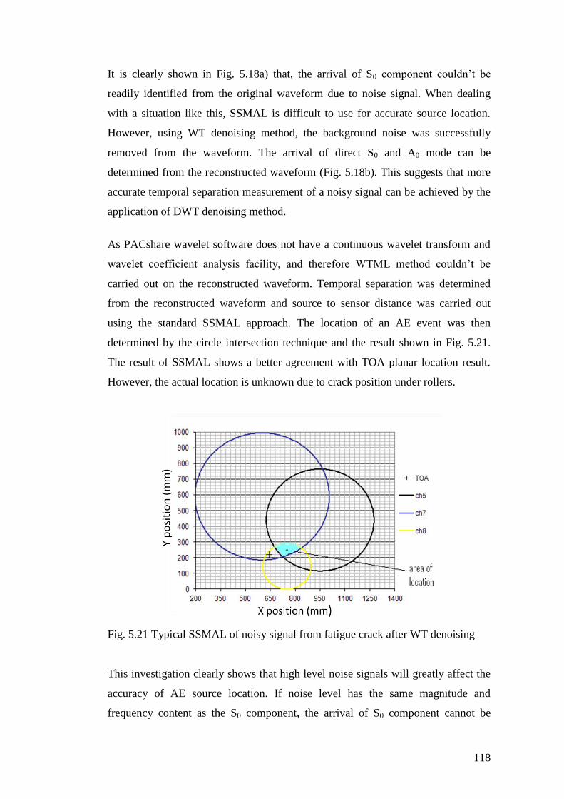
118
It is clearly shown in Fig. 5.18a) that, the arrival of S0 component couldn’t be
readily identified from the original waveform due to noise signal. When dealing
with a situation like this, SSMAL is difficult to use for accurate source location.
However, using WT denoising method, the background noise was successfully
removed from the waveform. The arrival of direct S0 and A0 mode can be
determined from the reconstructed waveform (Fig. 5.18b). This suggests that more
accurate temporal separation measurement of a noisy signal can be achieved by the
application of DWT denoising method.
As PACshare wavelet software does not have a continuous wavelet transform and
wavelet coefficient analysis facility, and therefore WTML method couldn’t be
carried out on the reconstructed waveform. Temporal separation was determined
from the reconstructed waveform and source to sensor distance was carried out
using the standard SSMAL approach. The location of an AE event was then
determined by the circle intersection technique and the result shown in Fig. 5.21.
The result of SSMAL shows a better agreement with TOA planar location result.
However, the actual location is unknown due to crack position under rollers.
Fig. 5.21 Typical SSMAL of noisy signal from fatigue crack after WT denoising
This investigation clearly shows that high level noise signals will greatly affect the
accuracy of AE source location. If noise level has the same magnitude and
frequency content as the S0 component, the arrival of S0 component cannot be
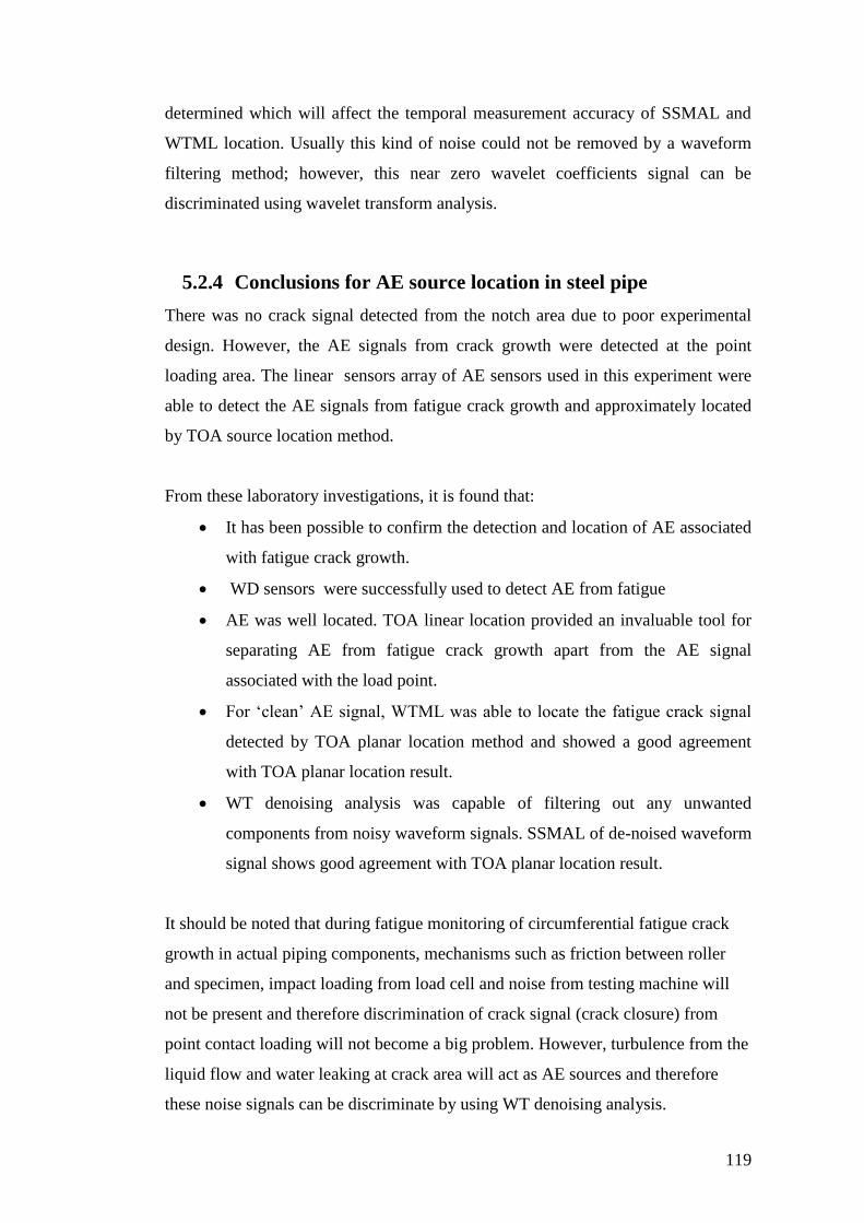
119
determined which will affect the temporal measurement accuracy of SSMAL and
WTML location. Usually this kind of noise could not be removed by a waveform
filtering method; however, this near zero wavelet coefficients signal can be
discriminated using wavelet transform analysis.
5.2.4 Conclusions for AE source location in steel pipe
There was no crack signal detected from the notch area due to poor experimental
design. However, the AE signals from crack growth were detected at the point
loading area. The linear sensors array of AE sensors used in this experiment were
able to detect the AE signals from fatigue crack growth and approximately located
by TOA source location method.
From these laboratory investigations, it is found that:
It has been possible to confirm the detection and location of AE associated
with fatigue crack growth.
WD sensors were successfully used to detect AE from fatigue
AE was well located. TOA linear location provided an invaluable tool for
separating AE from fatigue crack growth apart from the AE signal
associated with the load point.
For ‘clean’ AE signal, WTML was able to locate the fatigue crack signal
detected by TOA planar location method and showed a good agreement
with TOA planar location result.
WT denoising analysis was capable of filtering out any unwanted
components from noisy waveform signals. SSMAL of de-noised waveform
signal shows good agreement with TOA planar location result.
It should be noted that during fatigue monitoring of circumferential fatigue crack
growth in actual piping components, mechanisms such as friction between roller
and specimen, impact loading from load cell and noise from testing machine will
not be present and therefore discrimination of crack signal (crack closure) from
point contact loading will not become a big problem. However, turbulence from the
liquid flow and water leaking at crack area will act as AE sources and therefore
these noise signals can be discriminate by using WT denoising analysis.

120
5.3 Crack length measurement in steel plate using WTML
method
This section discusses a fatigue crack growth study carried out on a mild steel plate
specimen in order to provide better understanding of the characteristics of AE
signals from fatigue under tensile-tensile cyclic loading and to validate the
workability of WTML method to accurately locating such damage.
This research work aimed to:
Grow the fatigue crack in the mild steel plate using cyclic tensile loading.
Confirm that fatigue in this mild steel plate can be detected using AE
techniques.
Locate AE from fatigue damage using TOA location with linear and planar
sensor arrays.
Implement WTML method to the AE signal from fatigue crack growth
detected by TOA planar location.
Evaluate the efficiency of WTML for locating the actual data from fatigue
crack growth in the pipe.
Evaluate the capability the AE methods to measure crack length due to
fatigue crack growth under tensile-tensile loading.
5.3.1 Specimen geometry
Mild steel plate with dimension of 5mm thick, 790 X 300 mm was used in this
study. Seven holes were produced at each ends of the specimen (Fig. 5.22) in order
to hold the specimen on the testing machine. Two sharp notches were introduced at
both edge of specimen.
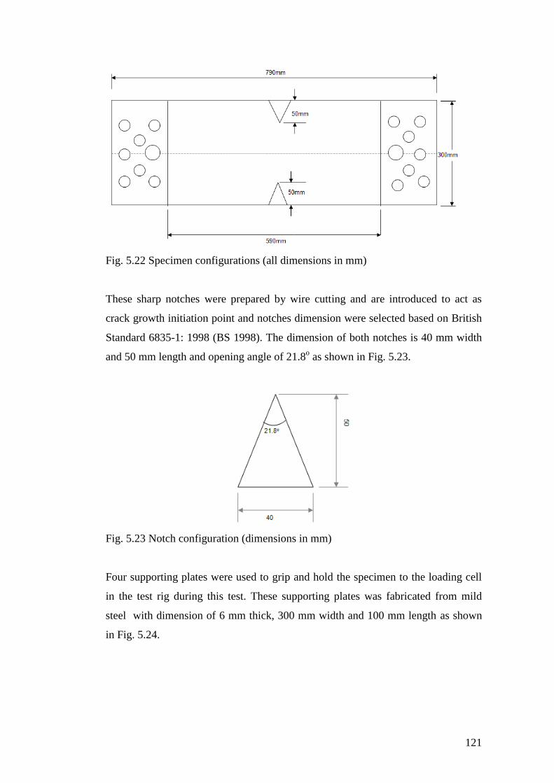
121
Fig. 5.22 Specimen configurations (all dimensions in mm)
These sharp notches were prepared by wire cutting and are introduced to act as
crack growth initiation point and notches dimension were selected based on British
Standard 6835-1: 1998 (BS 1998). The dimension of both notches is 40 mm width
and 50 mm length and opening angle of 21.8o as shown in Fig. 5.23.
Fig. 5.23 Notch configuration (dimensions in mm)
Four supporting plates were used to grip and hold the specimen to the loading cell
in the test rig during this test. These supporting plates was fabricated from mild
steel with dimension of 6 mm thick, 300 mm width and 100 mm length as shown
in Fig. 5.24.
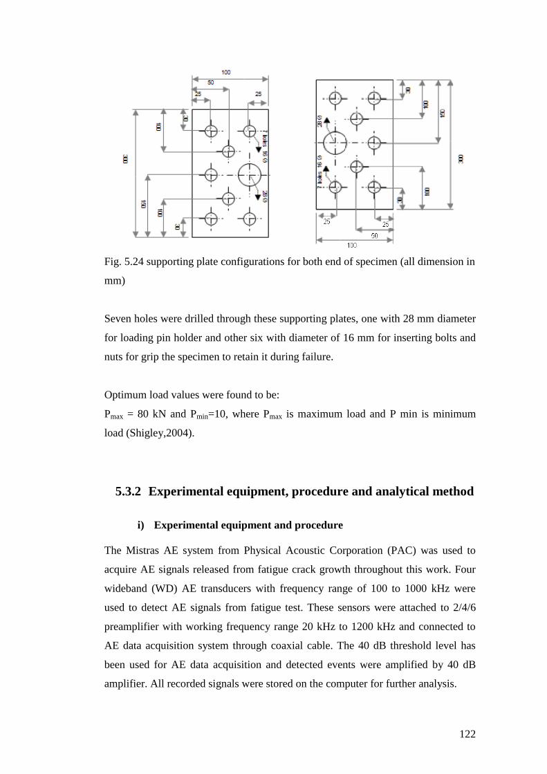
122
Fig. 5.24 supporting plate configurations for both end of specimen (all dimension in
mm)
Seven holes were drilled through these supporting plates, one with 28 mm diameter
for loading pin holder and other six with diameter of 16 mm for inserting bolts and
nuts for grip the specimen to retain it during failure.
Optimum load values were found to be:
Pmax = 80 kN and Pmin=10, where Pmax is maximum load and P min is minimum
load (Shigley,2004).
5.3.2 Experimental equipment, procedure and analytical method
i) Experimental equipment and procedure
The Mistras AE system from Physical Acoustic Corporation (PAC) was used to
acquire AE signals released from fatigue crack growth throughout this work. Four
wideband (WD) AE transducers with frequency range of 100 to 1000 kHz were
used to detect AE signals from fatigue test. These sensors were attached to 2/4/6
preamplifier with working frequency range 20 kHz to 1200 kHz and connected to
AE data acquisition system through coaxial cable. The 40 dB threshold level has
been used for AE data acquisition and detected events were amplified by 40 dB
amplifier. All recorded signals were stored on the computer for further analysis.
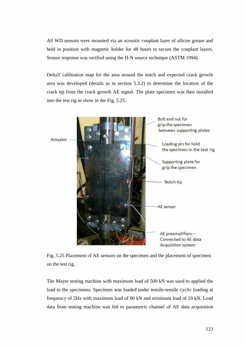
123
All WD sensors were mounted via an acoustic couplant layer of silicon grease and
held in position with magnetic holder for 48 hours to secure the couplant layers.
Sensor response was verified using the H-N source technique (ASTM 1994).
DeltaT calibration map for the area around the notch and expected crack growth
area was developed (details as in section 5.3.2) to determine the location of the
crack tip from the crack growth AE signal. The plate specimen was then installed
into the test rig as show in the Fig. 5.25.
Fig. 5.25 Placement of AE sensors on the specimen and the placement of specimen
on the test rig.
The Mayer testing machine with maximum load of 500 kN was used to applied the
load to the specimens. Specimen was loaded under tensile-tensile cyclic loading at
frequency of 2Hz with maximum load of 80 kN and minimum load of 10 kN. Load
data from testing machine was fed to parametric channel of AE data acquisition
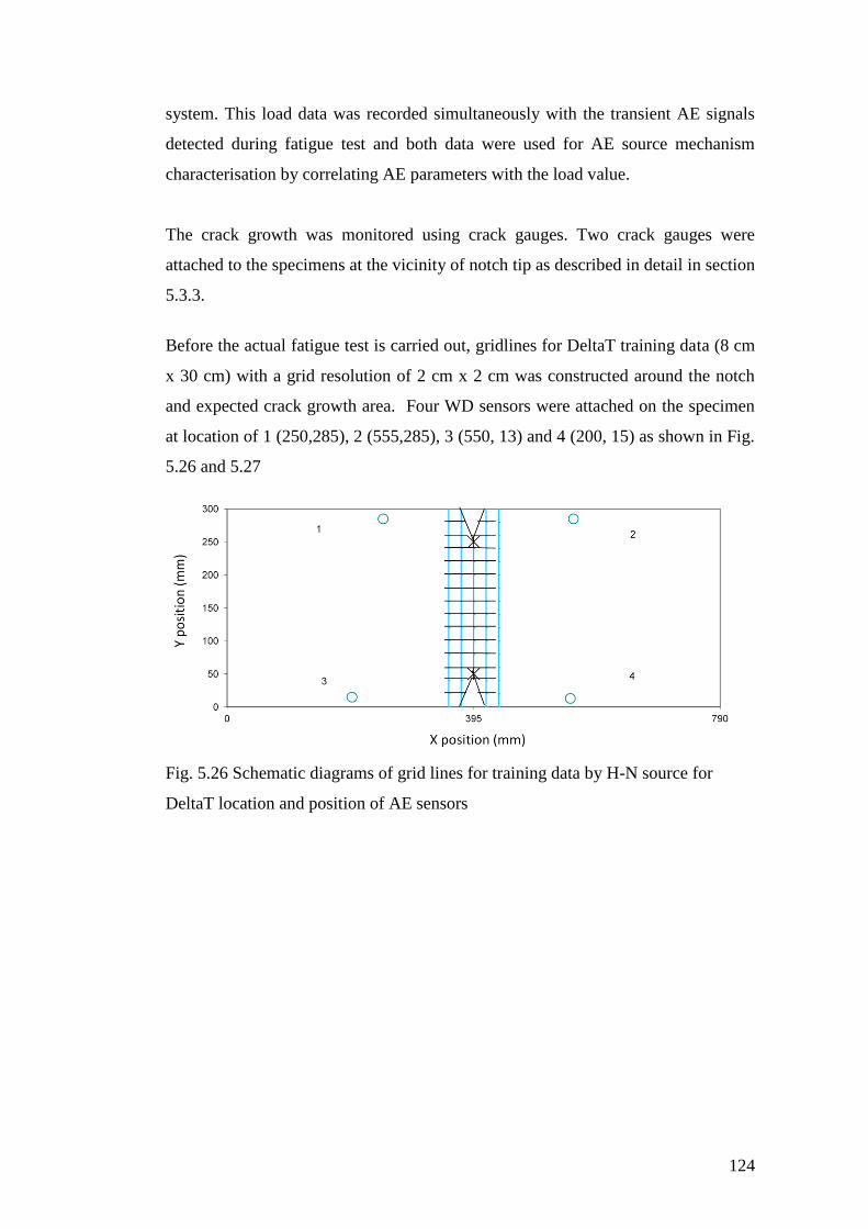
124
system. This load data was recorded simultaneously with the transient AE signals
detected during fatigue test and both data were used for AE source mechanism
characterisation by correlating AE parameters with the load value.
The crack growth was monitored using crack gauges. Two crack gauges were
attached to the specimens at the vicinity of notch tip as described in detail in section
5.3.3.
Before the actual fatigue test is carried out, gridlines for DeltaT training data (8 cm
x 30 cm) with a grid resolution of 2 cm x 2 cm was constructed around the notch
and expected crack growth area. Four WD sensors were attached on the specimen
at location of 1 (250,285), 2 (555,285), 3 (550, 13) and 4 (200, 15) as shown in Fig.
5.26 and 5.27
Fig. 5.26 Schematic diagrams of grid lines for training data by H-N source for
DeltaT location and position of AE sensors
125
Fig. 5.27 Actual grid line on the plate specimen
Five H-N sources were conducted at each node and time delays between each pair
of sensor were calculated using DeltaT software developed by Baxter (2007). The
DeltaT map base on time arrival delay between pairs of sensors was developed as
calibration map. Five H-N source were conducted at both notches and location of
this notch was compare with the calibration map to assess the performance of the
DeltaT map. This map will be used to determine the location of detected signal
during crack growth test using DeltaT approach and will be compared with other
location methods.
ii) Crack growth monitoring
Crack gauge as described in Chapter 3 (section 3.3.3) was used to monitor the crack
growth throughout this work. Crack gauge was attached to specimens at the vicinity
of notches tip. This gauge was connected to the power supply box and voltage
amplifier through a terminal as shown in Fig. 5.28.
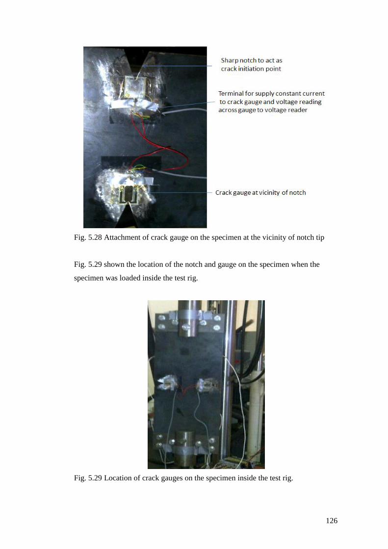
126
Fig. 5.28 Attachment of crack gauge on the specimen at the vicinity of notch tip
Fig. 5.29 shown the location of the notch and gauge on the specimen when the
specimen was loaded inside the test rig.
Fig. 5.29 Location of crack gauges on the specimen inside the test rig.
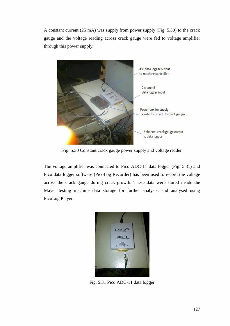
127
A constant current (25 mA) was supply from power supply (Fig. 5.30) to the crack
gauge and the voltage reading across crack gauge were fed to voltage amplifier
through this power supply.
Fig. 5.30 Constant crack gauge power supply and voltage reader
The voltage amplifier was connected to Pico ADC-11 data logger (Fig. 5.31) and
Pico data logger software (PicoLog Recorder) has been used to record the voltage
across the crack gauge during crack growth. These data were stored inside the
Mayer testing machine data storage for further analysis, and analysed using
PicoLog Player.
Fig. 5.31 Pico ADC-11 data logger
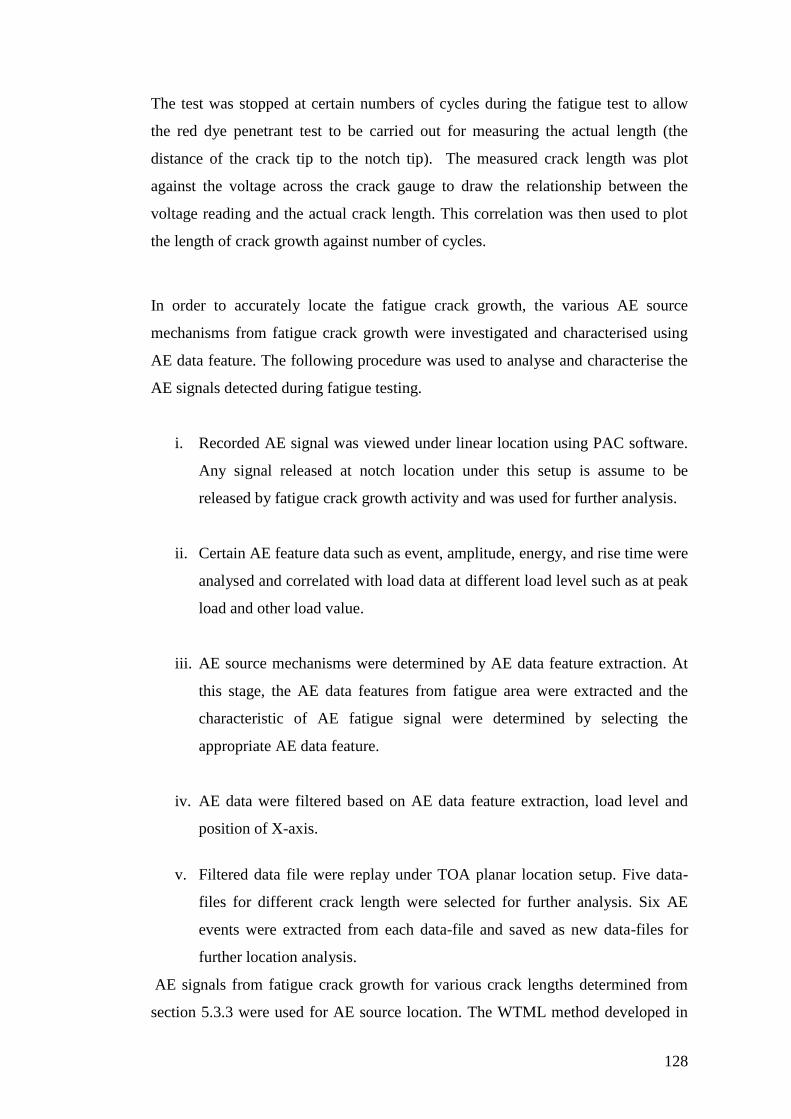
128
The test was stopped at certain numbers of cycles during the fatigue test to allow
the red dye penetrant test to be carried out for measuring the actual length (the
distance of the crack tip to the notch tip). The measured crack length was plot
against the voltage across the crack gauge to draw the relationship between the
voltage reading and the actual crack length. This correlation was then used to plot
the length of crack growth against number of cycles.
In order to accurately locate the fatigue crack growth, the various AE source
mechanisms from fatigue crack growth were investigated and characterised using
AE data feature. The following procedure was used to analyse and characterise the
AE signals detected during fatigue testing.
i. Recorded AE signal was viewed under linear location using PAC software.
Any signal released at notch location under this setup is assume to be
released by fatigue crack growth activity and was used for further analysis.
ii. Certain AE feature data such as event, amplitude, energy, and rise time were
analysed and correlated with load data at different load level such as at peak
load and other load value.
iii. AE source mechanisms were determined by AE data feature extraction. At
this stage, the AE data features from fatigue area were extracted and the
characteristic of AE fatigue signal were determined by selecting the
appropriate AE data feature.
iv. AE data were filtered based on AE data feature extraction, load level and
position of X-axis.
v. Filtered data file were replay under TOA planar location setup. Five data-
files for different crack length were selected for further analysis. Six AE
events were extracted from each data-file and saved as new data-files for
further location analysis.
AE signals from fatigue crack growth for various crack lengths determined from
section 5.3.3 were used for AE source location. The WTML method developed in
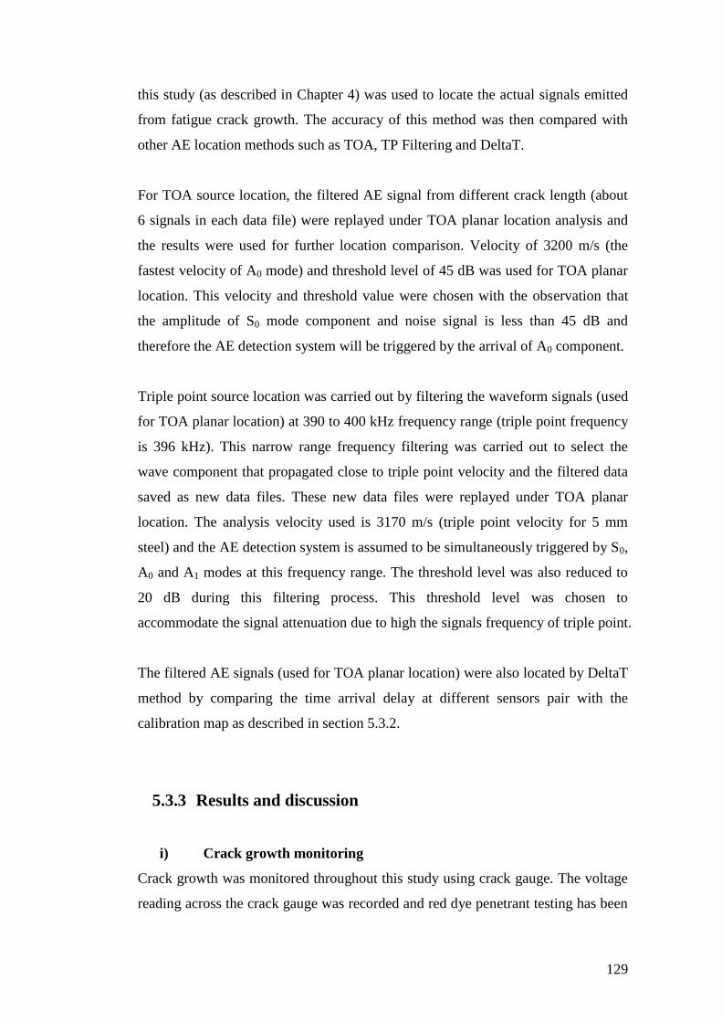
129
this study (as described in Chapter 4) was used to locate the actual signals emitted
from fatigue crack growth. The accuracy of this method was then compared with
other AE location methods such as TOA, TP Filtering and DeltaT.
For TOA source location, the filtered AE signal from different crack length (about
6 signals in each data file) were replayed under TOA planar location analysis and
the results were used for further location comparison. Velocity of 3200 m/s (the
fastest velocity of A0 mode) and threshold level of 45 dB was used for TOA planar
location. This velocity and threshold value were chosen with the observation that
the amplitude of S0 mode component and noise signal is less than 45 dB and
therefore the AE detection system will be triggered by the arrival of A0 component.
Triple point source location was carried out by filtering the waveform signals (used
for TOA planar location) at 390 to 400 kHz frequency range (triple point frequency
is 396 kHz). This narrow range frequency filtering was carried out to select the
wave component that propagated close to triple point velocity and the filtered data
saved as new data files. These new data files were replayed under TOA planar
location. The analysis velocity used is 3170 m/s (triple point velocity for 5 mm
steel) and the AE detection system is assumed to be simultaneously triggered by S0,
A0 and A1 modes at this frequency range. The threshold level was also reduced to
20 dB during this filtering process. This threshold level was chosen to
accommodate the signal attenuation due to high the signals frequency of triple point.
The filtered AE signals (used for TOA planar location) were also located by DeltaT
method by comparing the time arrival delay at different sensors pair with the
calibration map as described in section 5.3.2.
5.3.3 Results and discussion
i) Crack growth monitoring
Crack growth was monitored throughout this study using crack gauge. The voltage
reading across the crack gauge was recorded and red dye penetrant testing has been
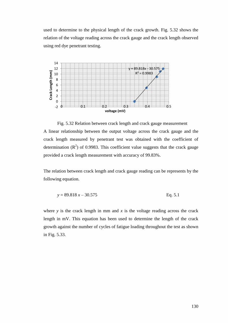
130
used to determine to the physical length of the crack growth. Fig. 5.32 shows the
relation of the voltage reading across the crack gauge and the crack length observed
using red dye penetrant testing.
Fig. 5.32 Relation between crack length and crack gauge measurement
A linear relationship between the output voltage across the crack gauge and the
crack length measured by penetrant test was obtained with the coefficient of
determination (R2) of 0.9983. This coefficient value suggests that the crack gauge
provided a crack length measurement with accuracy of 99.83%.
The relation between crack length and crack gauge reading can be represents by the
following equation.
y = 89.818 x – 30.575 Eq. 5.1
where y is the crack length in mm and x is the voltage reading across the crack
length in mV. This equation has been used to determine the length of the crack
growth against the number of cycles of fatigue loading throughout the test as shown
in Fig. 5.33.
y = 89.818x - 30.575 R² = 0.9983
-2
0
2
4
6
8
10
12
14
0 0.1 0.2 0.3 0.4 0.5
Cra
ck L
en
gth
(m
m)
voltage (mV)
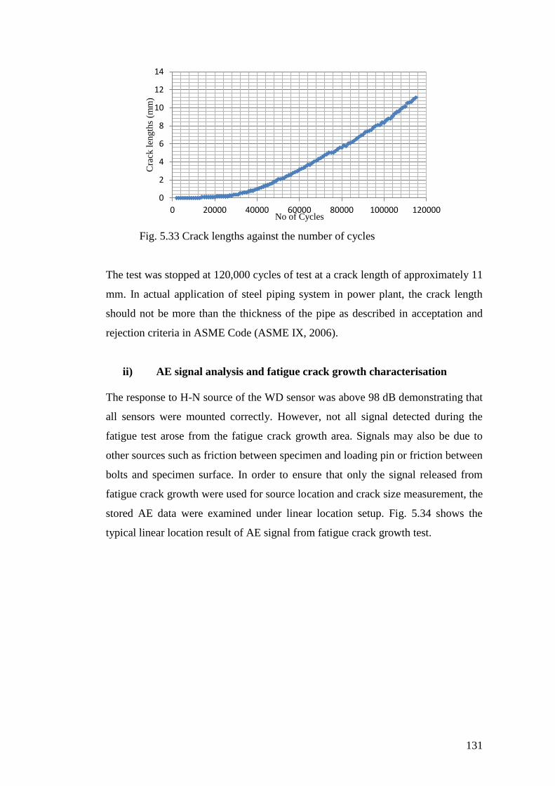
131
Fig. 5.33 Crack lengths against the number of cycles
The test was stopped at 120,000 cycles of test at a crack length of approximately 11
mm. In actual application of steel piping system in power plant, the crack length
should not be more than the thickness of the pipe as described in acceptation and
rejection criteria in ASME Code (ASME IX, 2006).
ii) AE signal analysis and fatigue crack growth characterisation
The response to H-N source of the WD sensor was above 98 dB demonstrating that
all sensors were mounted correctly. However, not all signal detected during the
fatigue test arose from the fatigue crack growth area. Signals may also be due to
other sources such as friction between specimen and loading pin or friction between
bolts and specimen surface. In order to ensure that only the signal released from
fatigue crack growth were used for source location and crack size measurement, the
stored AE data were examined under linear location setup. Fig. 5.34 shows the
typical linear location result of AE signal from fatigue crack growth test.
0
2
4
6
8
10
12
14
0 20000 40000 60000 80000 100000 120000
Cra
ck l
ength
s (m
m)
No of Cycles
132
Fig. 5.34 Plot of cumulative AE event against X position
This linear location result shows a very good agreement with the actual notch
location (395, 250) which suggest that the detected AE signal were emitted by
fatigue crack growth activity in the vicinity of the notch tip.
According to Scruby (1987), the primary sources associated with crack growth are
plastic zone extension, plastic opening at the crack tip and elastic crack advance.
However, plastic zone extension and plastic opening at the crack tip may not be
detectable under slow ductile loading and elastic crack advance can be detected if
their mechanism is fast brittle fracture. Most of these sources are generated at peak
load value under cyclic fatigue loading.
Secondary events associated with fatigue crack growth are crack face fretting
(Scruby 1987). This mechanism also known as crack closure and usually occurs at
lower load value (Pollock 2012).
Since the source mechanism of fatigue crack growth is load dependent, load level
of detected AE signals was plotted against the duration of test and Fig. 5.35 shows
a typical plot of load level of detected signals versus test duration from one of
recorded AE data-file.
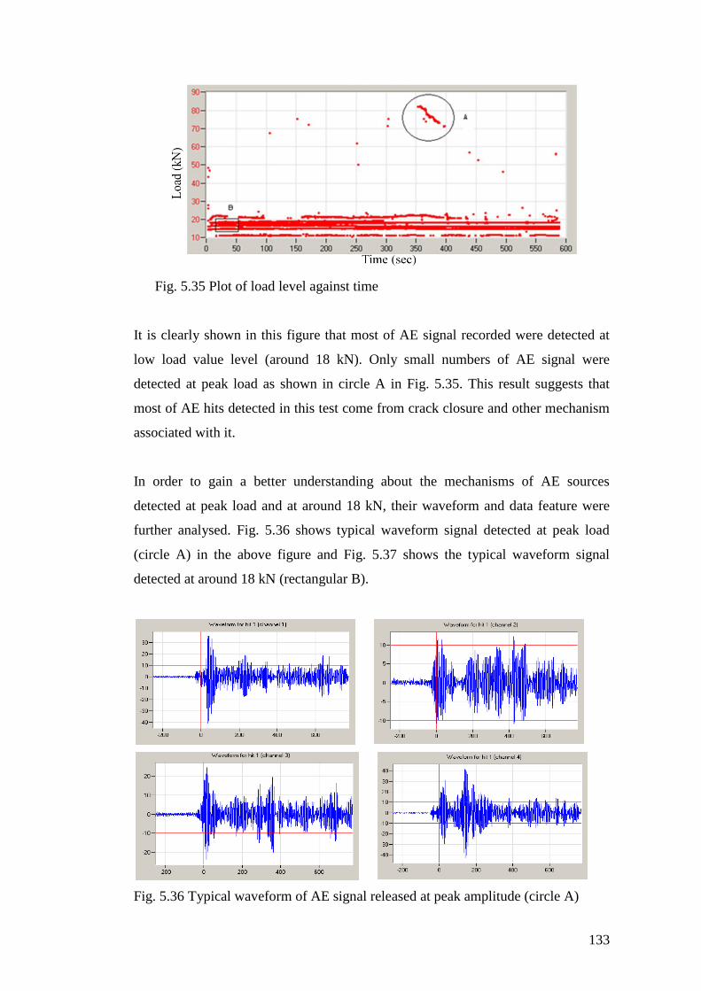
133
Fig. 5.35 Plot of load level against time
It is clearly shown in this figure that most of AE signal recorded were detected at
low load value level (around 18 kN). Only small numbers of AE signal were
detected at peak load as shown in circle A in Fig. 5.35. This result suggests that
most of AE hits detected in this test come from crack closure and other mechanism
associated with it.
In order to gain a better understanding about the mechanisms of AE sources
detected at peak load and at around 18 kN, their waveform and data feature were
further analysed. Fig. 5.36 shows typical waveform signal detected at peak load
(circle A) in the above figure and Fig. 5.37 shows the typical waveform signal
detected at around 18 kN (rectangular B).
Fig. 5.36 Typical waveform of AE signal released at peak amplitude (circle A)
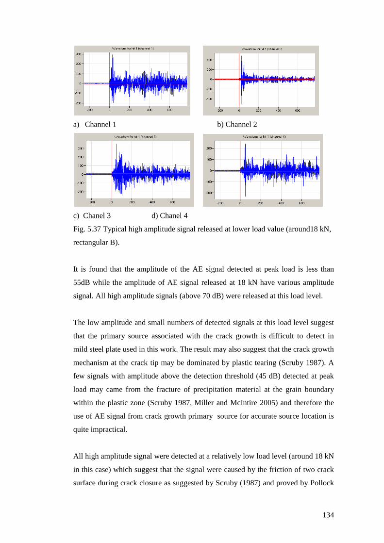
134
a) Channel 1 b) Channel 2
c) Chanel 3 d) Chanel 4
Fig. 5.37 Typical high amplitude signal released at lower load value (around18 kN,
rectangular B).
It is found that the amplitude of the AE signal detected at peak load is less than
55dB while the amplitude of AE signal released at 18 kN have various amplitude
signal. All high amplitude signals (above 70 dB) were released at this load level.
The low amplitude and small numbers of detected signals at this load level suggest
that the primary source associated with the crack growth is difficult to detect in
mild steel plate used in this work. The result may also suggest that the crack growth
mechanism at the crack tip may be dominated by plastic tearing (Scruby 1987). A
few signals with amplitude above the detection threshold (45 dB) detected at peak
load may came from the fracture of precipitation material at the grain boundary
within the plastic zone (Scruby 1987, Miller and McIntire 2005) and therefore the
use of AE signal from crack growth primary source for accurate source location is
quite impractical.
All high amplitude signal were detected at a relatively low load level (around 18 kN
in this case) which suggest that the signal were caused by the friction of two crack
surface during crack closure as suggested by Scruby (1987) and proved by Pollock
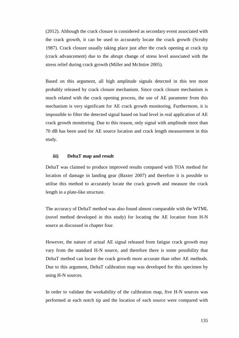
135
(2012). Although the crack closure is considered as secondary event associated with
the crack growth, it can be used to accurately locate the crack growth (Scruby
1987). Crack closure usually taking place just after the crack opening at crack tip
(crack advancement) due to the abrupt change of stress level associated with the
stress relief during crack growth (Miller and McIntire 2005).
Based on this argument, all high amplitude signals detected in this test most
probably released by crack closure mechanism. Since crack closure mechanism is
much related with the crack opening process, the use of AE parameter from this
mechanism is very significant for AE crack growth monitoring. Furthermore, it is
impossible to filter the detected signal based on load level in real application of AE
crack growth monitoring. Due to this reason, only signal with amplitude more than
70 dB has been used for AE source location and crack length measurement in this
study.
iii) DeltaT map and result
DeltaT was claimed to produce improved results compared with TOA method for
location of damage in landing gear (Baxter 2007) and therefore it is possible to
utilise this method to accurately locate the crack growth and measure the crack
length in a plate-like structure.
The accuracy of DeltaT method was also found almost comparable with the WTML
(novel method developed in this study) for locating the AE location from H-N
source as discussed in chapter four.
However, the nature of actual AE signal released from fatigue crack growth may
vary from the standard H-N source, and therefore there is some possibility that
DeltaT method can locate the crack growth more accurate than other AE methods.
Due to this argument, DeltaT calibration map was developed for this specimen by
using H-N sources.
In order to validate the workability of the calibration map, five H-N sources was
performed at each notch tip and the location of each source were compared with
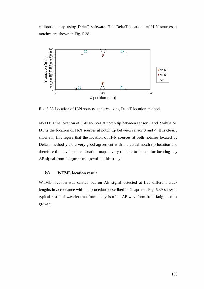
136
calibration map using DeltaT software. The DeltaT locations of H-N sources at
notches are shown in Fig. 5.38.
Fig. 5.38 Location of H-N sources at notch using DeltaT location method.
N5 DT is the location of H-N sources at notch tip between sensor 1 and 2 while N6
DT is the location of H-N sources at notch tip between sensor 3 and 4. It is clearly
shown in this figure that the location of H-N sources at both notches located by
DeltaT method yield a very good agreement with the actual notch tip location and
therefore the developed calibration map is very reliable to be use for locating any
AE signal from fatigue crack growth in this study.
iv) WTML location result
WTML location was carried out on AE signal detected at five different crack
lengths in accordance with the procedure described in Chapter 4. Fig. 5.39 shows a
typical result of wavelet transform analysis of an AE waveform from fatigue crack
growth.
0 20 40 60 80
100 120 140 160 180 200 220 240 260 280 300
0 395 790
Y p
ositio
n (
mm
)
X position (mm)
N5 DT
N6 DT
act
1 2
3 4
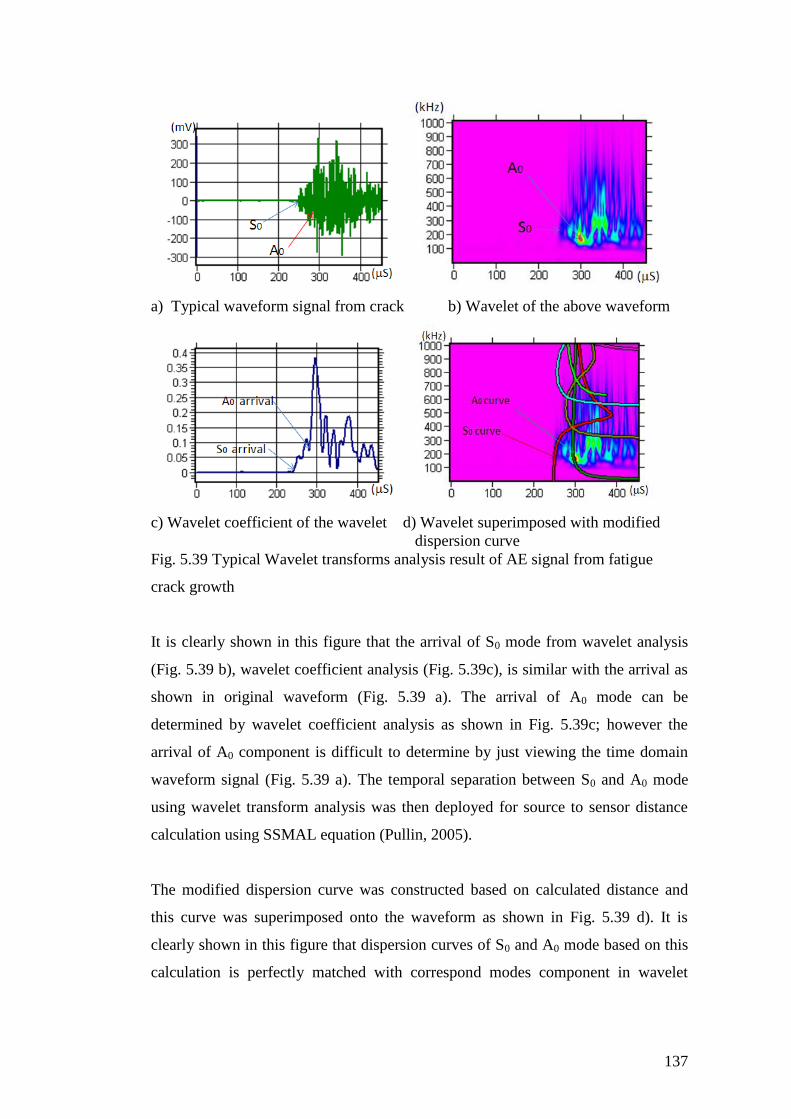
137
a) Typical waveform signal from crack b) Wavelet of the above waveform
c) Wavelet coefficient of the wavelet d) Wavelet superimposed with modified
dispersion curve
Fig. 5.39 Typical Wavelet transforms analysis result of AE signal from fatigue
crack growth
It is clearly shown in this figure that the arrival of S0 mode from wavelet analysis
(Fig. 5.39 b), wavelet coefficient analysis (Fig. 5.39c), is similar with the arrival as
shown in original waveform (Fig. 5.39 a). The arrival of A0 mode can be
determined by wavelet coefficient analysis as shown in Fig. 5.39c; however the
arrival of A0 component is difficult to determine by just viewing the time domain
waveform signal (Fig. 5.39 a). The temporal separation between S0 and A0 mode
using wavelet transform analysis was then deployed for source to sensor distance
calculation using SSMAL equation (Pullin, 2005).
The modified dispersion curve was constructed based on calculated distance and
this curve was superimposed onto the waveform as shown in Fig. 5.39 d). It is
clearly shown in this figure that dispersion curves of S0 and A0 mode based on this
calculation is perfectly matched with correspond modes component in wavelet
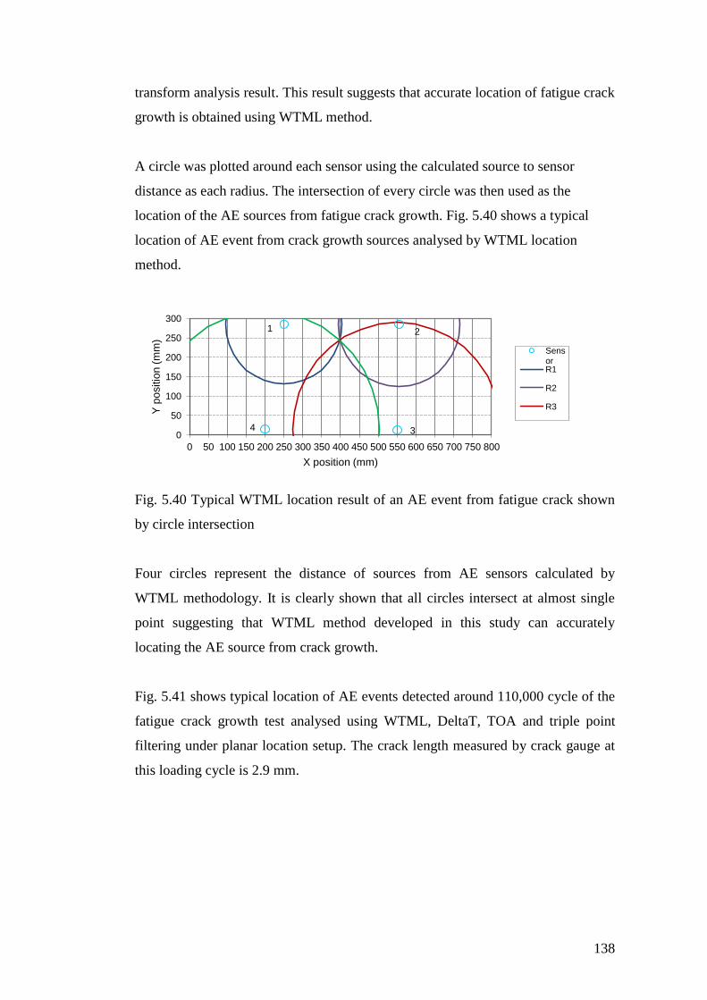
138
transform analysis result. This result suggests that accurate location of fatigue crack
growth is obtained using WTML method.
A circle was plotted around each sensor using the calculated source to sensor
distance as each radius. The intersection of every circle was then used as the
location of the AE sources from fatigue crack growth. Fig. 5.40 shows a typical
location of AE event from crack growth sources analysed by WTML location
method.
Fig. 5.40 Typical WTML location result of an AE event from fatigue crack shown
by circle intersection
Four circles represent the distance of sources from AE sensors calculated by
WTML methodology. It is clearly shown that all circles intersect at almost single
point suggesting that WTML method developed in this study can accurately
locating the AE source from crack growth.
Fig. 5.41 shows typical location of AE events detected around 110,000 cycle of the
fatigue crack growth test analysed using WTML, DeltaT, TOA and triple point
filtering under planar location setup. The crack length measured by crack gauge at
this loading cycle is 2.9 mm.
0
50
100
150
200
250
300
0 50 100 150 200 250 300 350 400 450 500 550 600 650 700 750 800
Y p
ositio
n (
mm
)
X position (mm)
Sensor R1
R2
R3
1 2
3 4
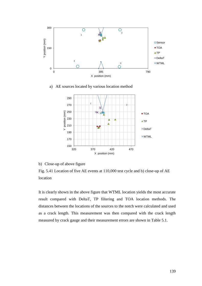
139
a) AE sources located by various location method
b) Close-up of above figure
Fig. 5.41 Location of five AE events at 110,000 test cycle and b) close-up of AE
location
It is clearly shown in the above figure that WTML location yields the most accurate
result compared with DeltaT, TP filtering and TOA location methods. The
distances between the locations of the sources to the notch were calculated and used
as a crack length. This measurement was then compared with the crack length
measured by crack gauge and their measurement errors are shown in Table 5.1.
0
150
300
0 395 790
Y p
ositio
n (
mm
)
X position (mm)
Sensor
TOA
TP
DeltaT
WTML
1 2
4
3
150
170
190
210
230
250
270
290
320 370 420 470
Y positio
n (
mm
)
X position (mm)
TOA
TP
DeltaT
WTML
1 2
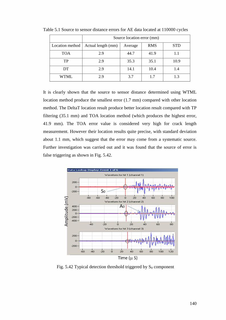
140
Table 5.1 Source to sensor distance errors for AE data located at 110000 cycles
Source location error (mm)
Location method Actual length (mm) Average RMS STD
TOA 2.9 44.7 41.9 1.1
TP 2.9 35.3 35.1 10.9
DT 2.9 14.1 10.4 1.4
WTML 2.9 3.7 1.7 1.3
It is clearly shown that the source to sensor distance determined using WTML
location method produce the smallest error (1.7 mm) compared with other location
method. The DeltaT location result produce better location result compared with TP
filtering (35.1 mm) and TOA location method (which produces the highest error,
41.9 mm). The TOA error value is considered very high for crack length
measurement. However their location results quite precise, with standard deviation
about 1.1 mm, which suggest that the error may come from a systematic source.
Further investigation was carried out and it was found that the source of error is
false triggering as shown in Fig. 5.42.
Fig. 5.42 Typical detection threshold triggered by S0 component
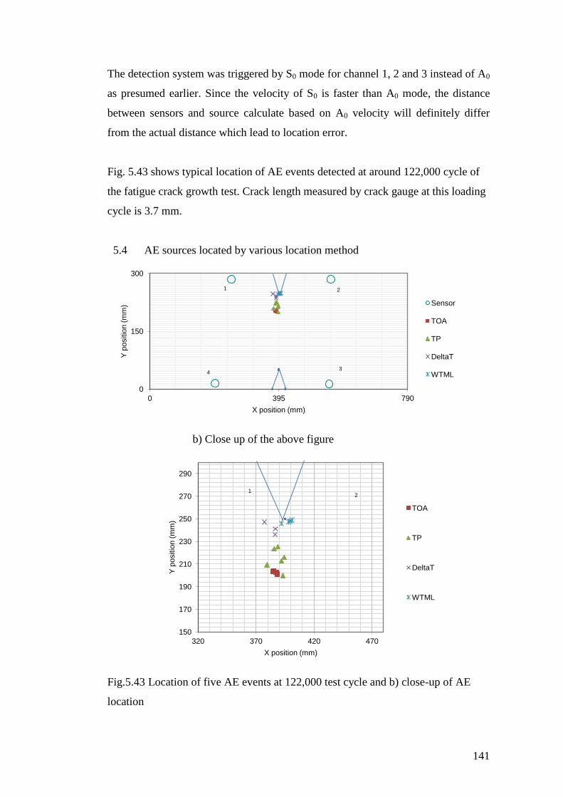
141
The detection system was triggered by S0 mode for channel 1, 2 and 3 instead of A0
as presumed earlier. Since the velocity of S0 is faster than A0 mode, the distance
between sensors and source calculate based on A0 velocity will definitely differ
from the actual distance which lead to location error.
Fig. 5.43 shows typical location of AE events detected at around 122,000 cycle of
the fatigue crack growth test. Crack length measured by crack gauge at this loading
cycle is 3.7 mm.
5.4 AE sources located by various location method
b) Close up of the above figure
Fig.5.43 Location of five AE events at 122,000 test cycle and b) close-up of AE
location
0
150
300
0 395 790
Y p
ositio
n (
mm
)
X position (mm)
Sensor
TOA
TP
DeltaT
WTML
1 2
4 3
150
170
190
210
230
250
270
290
320 370 420 470
Y p
ositio
n (
mm
)
X position (mm)
TOA
TP
DeltaT
WTML
1 2
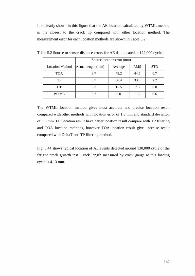
142
It is clearly shown in this figure that the AE location calculated by WTML method
is the closest to the crack tip compared with other location method. The
measurement error for each location methods are shown in Table 5.2.
Table 5.2 Source to sensor distance errors for AE data located at 122,000 cycles
Source location error (mm)
Location Method Actual length (mm) Average RMS STD
TOA 3.7 48.2 44.5 0.7
TP 3.7 36.4 33.8 7.2
DT 3.7 15.5 7.8 6.0
WTML 3.7 5.0 1.3 0.6
The WTML location method gives most accurate and precise location result
compared with other methods with location error of 1.3 mm and standard deviation
of 0.6 mm. DT location result have better location result compare with TP filtering
and TOA location methods, however TOA location result give precise result
compared with DeltaT and TP filtering method.
Fig. 5.44 shows typical location of AE events detected around 130,000 cycle of the
fatigue crack growth test. Crack length measured by crack gauge at this loading
cycle is 4.13 mm.
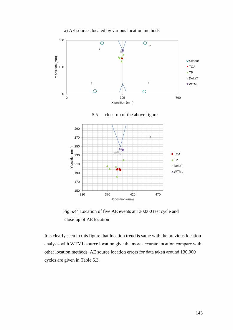
143
a) AE sources located by various location methods
5.5 close-up of the above figure
Fig.5.44 Location of five AE events at 130,000 test cycle and
close-up of AE location
It is clearly seen in this figure that location trend is same with the previous location
analysis with WTML source location give the more accurate location compare with
other location methods. AE source location errors for data taken around 130,000
cycles are given in Table 5.3.
0
150
300
0 395 790
Y p
ositio
n (
mm
)
X position (mm)
Sensor
TOA
TP
DeltaT
WTML
1
2
4 3
150
170
190
210
230
250
270
290
320 370 420 470
Y p
ositio
n (
mm
)
X position (mm)
TOA
TP
DeltaT
WTML
1 2
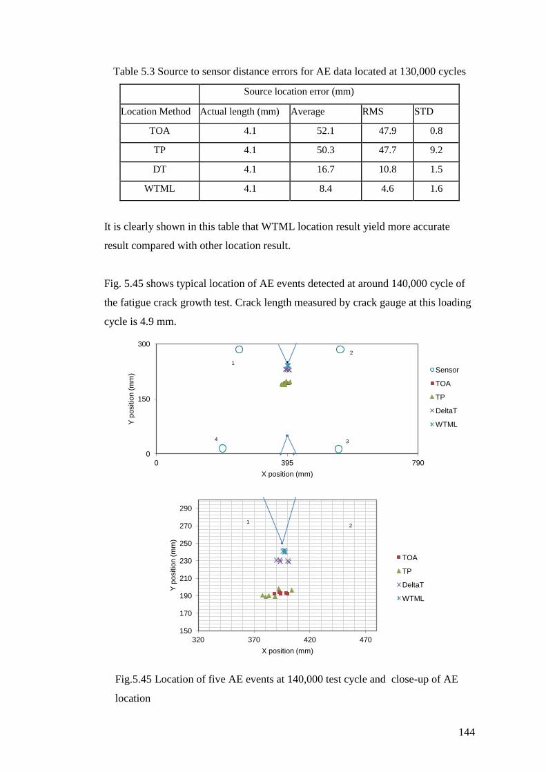
144
Table 5.3 Source to sensor distance errors for AE data located at 130,000 cycles
Source location error (mm)
Location Method Actual length (mm) Average RMS STD
TOA 4.1 52.1 47.9 0.8
TP 4.1 50.3 47.7 9.2
DT 4.1 16.7 10.8 1.5
WTML 4.1 8.4 4.6 1.6
It is clearly shown in this table that WTML location result yield more accurate
result compared with other location result.
Fig. 5.45 shows typical location of AE events detected at around 140,000 cycle of
the fatigue crack growth test. Crack length measured by crack gauge at this loading
cycle is 4.9 mm.
Fig.5.45 Location of five AE events at 140,000 test cycle and close-up of AE
location
0
150
300
0 395 790
Y p
ositio
n (
mm
)
X position (mm)
Sensor
TOA
TP
DeltaT
WTML
1
2
4 3
150
170
190
210
230
250
270
290
320 370 420 470
Y p
ositio
n (
mm
)
X position (mm)
TOA
TP
DeltaT
WTML
1 2
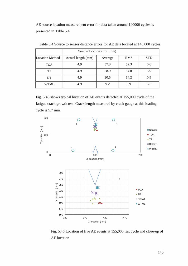
145
AE source location measurement error for data taken around 140000 cycles is
presented in Table 5.4.
Table 5.4 Source to sensor distance errors for AE data located at 140,000 cycles
Source location error (mm)
Location Method Actual length (mm) Average RMS STD
TOA 4.9 57.3 52.3 0.6
TP 4.9 58.9 54.0 3.9
DT 4.9 20.5 14.2 0.9
WTML 4.9 9.2 3.9 5.5
Fig. 5.46 shows typical location of AE events detected at 155,000 cycle of the
fatigue crack growth test. Crack length measured by crack gauge at this loading
cycle is 5.7 mm.
Fig. 5.46 Location of five AE events at 155,000 test cycle and close-up of
AE location
0
150
300
0 395 790
Y p
ositio
n (
mm
)
X position (mm)
Sensor
TOA
TP
DeltaT
WTML
1 2
4 3
150
170
190
210
230
250
270
290
320 370 420 470
Y lo
catio
n (
mm
)
X location (mm)
TOA
TP
DeltaT
WTML
1 2
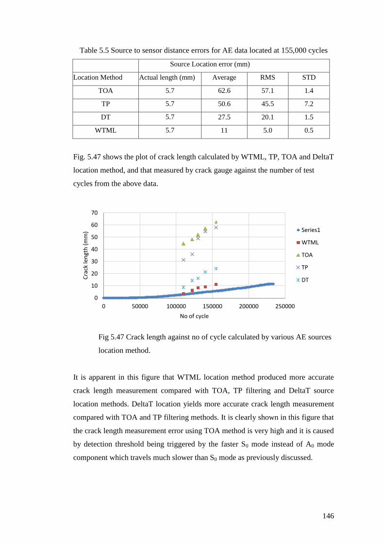
146
Table 5.5 Source to sensor distance errors for AE data located at 155,000 cycles
Source Location error (mm)
Location Method Actual length (mm) Average RMS STD
TOA 5.7 62.6 57.1 1.4
TP 5.7 50.6 45.5 7.2
DT 5.7 27.5 20.1 1.5
WTML 5.7 11 5.0 0.5
Fig. 5.47 shows the plot of crack length calculated by WTML, TP, TOA and DeltaT
location method, and that measured by crack gauge against the number of test
cycles from the above data.
Fig 5.47 Crack length against no of cycle calculated by various AE sources
location method.
It is apparent in this figure that WTML location method produced more accurate
crack length measurement compared with TOA, TP filtering and DeltaT source
location methods. DeltaT location yields more accurate crack length measurement
compared with TOA and TP filtering methods. It is clearly shown in this figure that
the crack length measurement error using TOA method is very high and it is caused
by detection threshold being triggered by the faster S0 mode instead of A0 mode
component which travels much slower than S0 mode as previously discussed.
0
10
20
30
40
50
60
70
0 50000 100000 150000 200000 250000
Cra
ck le
ngt
h (
mm
)
No of cycle
Series1
WTML
TOA
TP
DT
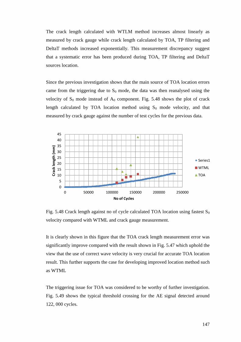
147
The crack length calculated with WTLM method increases almost linearly as
measured by crack gauge while crack length calculated by TOA, TP filtering and
DeltaT methods increased exponentially. This measurement discrepancy suggest
that a systematic error has been produced during TOA, TP filtering and DeltaT
sources location.
Since the previous investigation shows that the main source of TOA location errors
came from the triggering due to S0 mode, the data was then reanalysed using the
velocity of S0 mode instead of A0 component. Fig. 5.48 shows the plot of crack
length calculated by TOA location method using S0 mode velocity, and that
measured by crack gauge against the number of test cycles for the previous data.
Fig. 5.48 Crack length against no of cycle calculated TOA location using fastest S0
velocity compared with WTML and crack gauge measurement.
It is clearly shown in this figure that the TOA crack length measurement error was
significantly improve compared with the result shown in Fig. 5.47 which uphold the
view that the use of correct wave velocity is very crucial for accurate TOA location
result. This further supports the case for developing improved location method such
as WTML
The triggering issue for TOA was considered to be worthy of further investigation.
Fig. 5.49 shows the typical threshold crossing for the AE signal detected around
122, 000 cycles.
0
5
10
15
20
25
30
35
40
45
0 50000 100000 150000 200000 250000
Cra
ck le
ngt
h (
mm
)
No of Cycles
Series1
WTML
TOA
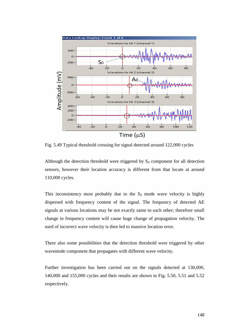
148
Fig. 5.49 Typical threshold crossing for signal detected around 122,000 cycles
Although the detection threshold were triggered by S0 component for all detection
sensors, however their location accuracy is different from that locate at around
110,000 cycles.
This inconsistency most probably due to the S0 mode wave velocity is highly
dispersed with frequency content of the signal. The frequency of detected AE
signals at various locations may be not exactly same to each other; therefore small
change in frequency content will cause huge change of propagation velocity. The
used of incorrect wave velocity is then led to massive location error.
There also some possibilities that the detection threshold were triggered by other
wavemode component that propagates with different wave velocity.
Further investigation has been carried out on the signals detected at 130,000,
140,000 and 155,000 cycles and their results are shown in Fig. 5.50, 5.51 and 5.52
respectively.
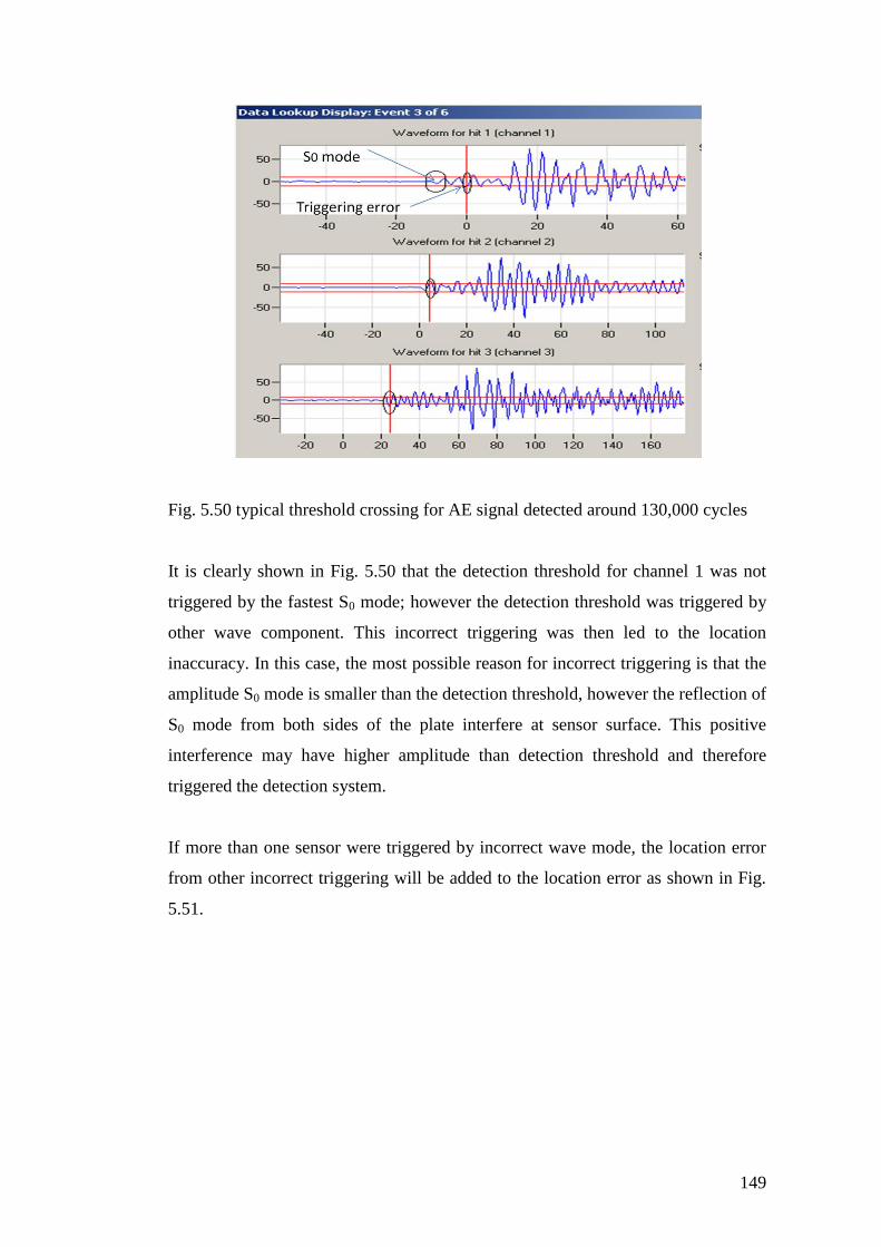
149
Fig. 5.50 typical threshold crossing for AE signal detected around 130,000 cycles
It is clearly shown in Fig. 5.50 that the detection threshold for channel 1 was not
triggered by the fastest S0 mode; however the detection threshold was triggered by
other wave component. This incorrect triggering was then led to the location
inaccuracy. In this case, the most possible reason for incorrect triggering is that the
amplitude S0 mode is smaller than the detection threshold, however the reflection of
S0 mode from both sides of the plate interfere at sensor surface. This positive
interference may have higher amplitude than detection threshold and therefore
triggered the detection system.
If more than one sensor were triggered by incorrect wave mode, the location error
from other incorrect triggering will be added to the location error as shown in Fig.
5.51.
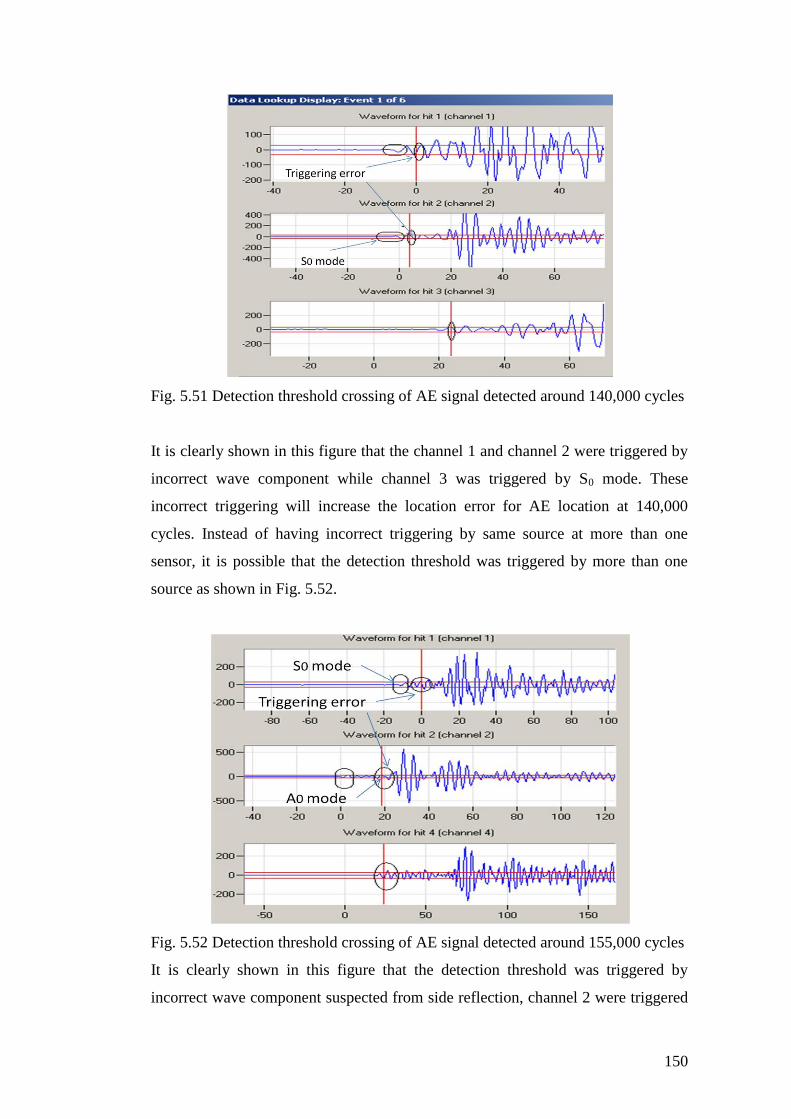
150
Fig. 5.51 Detection threshold crossing of AE signal detected around 140,000 cycles
It is clearly shown in this figure that the channel 1 and channel 2 were triggered by
incorrect wave component while channel 3 was triggered by S0 mode. These
incorrect triggering will increase the location error for AE location at 140,000
cycles. Instead of having incorrect triggering by same source at more than one
sensor, it is possible that the detection threshold was triggered by more than one
source as shown in Fig. 5.52.
Fig. 5.52 Detection threshold crossing of AE signal detected around 155,000 cycles
It is clearly shown in this figure that the detection threshold was triggered by
incorrect wave component suspected from side reflection, channel 2 were triggered
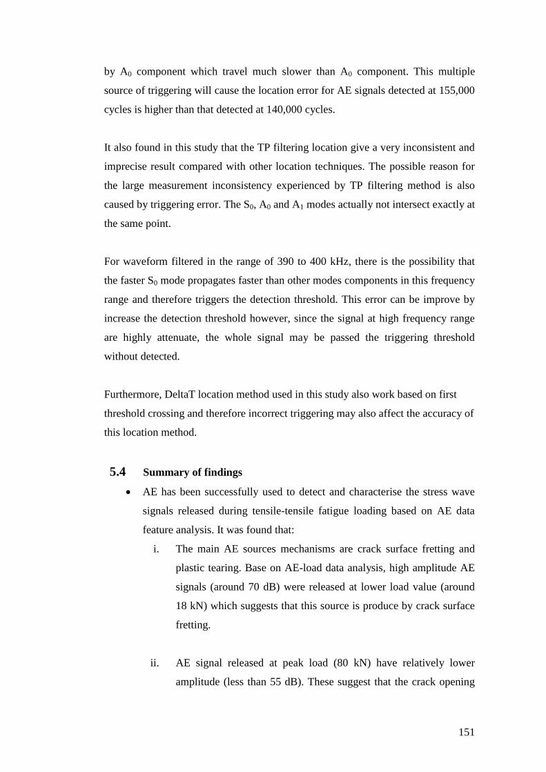
151
by A0 component which travel much slower than A0 component. This multiple
source of triggering will cause the location error for AE signals detected at 155,000
cycles is higher than that detected at 140,000 cycles.
It also found in this study that the TP filtering location give a very inconsistent and
imprecise result compared with other location techniques. The possible reason for
the large measurement inconsistency experienced by TP filtering method is also
caused by triggering error. The S0, A0 and A1 modes actually not intersect exactly at
the same point.
For waveform filtered in the range of 390 to 400 kHz, there is the possibility that
the faster S0 mode propagates faster than other modes components in this frequency
range and therefore triggers the detection threshold. This error can be improve by
increase the detection threshold however, since the signal at high frequency range
are highly attenuate, the whole signal may be passed the triggering threshold
without detected.
Furthermore, DeltaT location method used in this study also work based on first
threshold crossing and therefore incorrect triggering may also affect the accuracy of
this location method.
5.4 Summary of findings
AE has been successfully used to detect and characterise the stress wave
signals released during tensile-tensile fatigue loading based on AE data
feature analysis. It was found that:
i. The main AE sources mechanisms are crack surface fretting and
plastic tearing. Base on AE-load data analysis, high amplitude AE
signals (around 70 dB) were released at lower load value (around
18 kN) which suggests that this source is produce by crack surface
fretting.
ii. AE signal released at peak load (80 kN) have relatively lower
amplitude (less than 55 dB). These suggest that the crack opening
152
mechanisms during fatigue crack growth is tearing of plastic
deformation area in the vicinity of the crack tip.
WTML was successfully used to accurately locate the AE signal released
from fatigue crack growth. The accuracy of WTML is much better than
TOA, DeltaT and triple point filtering location methods.
WTML was successfully used to determine the crack length in the steel
pipe with the maximum measurement error of 5 mm. A step by step guide
to WTML methodology to measure the crack length is shown in Appendix
1
WTML based location technique can be used to measure crack length if
accurate enough.
The TOA location method produces the largest location inaccuracy. The
main sources of location errors are triggering error and therefore TOA
planar location based on threshold crossing is not reliable to be used for
accurately measure the fatigue crack length.
153
CHAPTER 6: CONCLUSIONS AND FUTURE WORKS
Managing the safety aspect of ageing nuclear power plant is very important to
ensure their integrity and functional capability is achieved throughout the entire
plant service life. Thermal fatigue is among the major ageing mechanism in nuclear
power plant piping system and a through wall crack and leakage are the most likely
modes of failure. Acoustic emission (AE) testing can be used to globally locate an
active source emitted from cracking area by using an array of sensors.
The cost saving of deploying an AE inspection method can be achieved by
minimisation of the time to perform the follow up test due to the localisation of the
damage source and the downtime associated with plant shut down.
6.1 Summary of Conclusion
An accurate AE source location methodology has been developed in this work
using wavelet transform analysis (WT) and modal location theory. This new
method is known as Wavelet Transform analysis and Modal Location (WTML).
This novel method utilised the dispersive characteristic of Lamb waves and time-
frequency discrimination capability of wavelet transform analysis.
It is possible to use AE technology for measuring the crack length in steel pipes
based on the proposed location method. The accuracy of WTML is found to be
superior to other AE location methods.
6.1.1 WT Source location of H-N source in steel plate and pipe
Novel WTML method has been successfully developed. This method
utilised modal location theory (velocity of different wave component) and
time-frequency discrimination capability of wavelet transform analysis.
154
It is found that WTML is more accurate than conventional TOA. WTML
overcomes false threshold triggering and time delay between first arrival
and first threshold crossing.
WTML is more accurate than TP filtering. TP is expected to produce
more accurate source location than FTC TOA since the detection
threshold is triggered by S0, A0 and A1 simultaneously. However, TP
occurs at relatively higher frequency at which AE signal highly attenuate,
increase the time delay between FTC and first arrival which lead to
location inaccuracy.
WTML improve the accuracy of SSMAL due to the time-frequency
discrimination capability of WT analysis which improves the temporal
separation measurement error.
WTML is comparable with DeltaT in term of accuracy, however it is
considered superior since the proposed method does not requires
calibration of testing area and the sensors can be moved anywhere on the
test item. Furthermore, single sensor WTML for monitoring crack growth
in nuclear piping especially circumferential crack in welded area is
possible.
6.1.2 WT Source location for fatigue crack growth in steel plate
AE has been successfully used to detect and characterise the stress wave
signals released during tensile-tensile fatigue loading based on AE data
feature analysis. It was found that:
o The main AE source mechanisms are crack surface fretting and
plastic tearing. Base on AE-load data analysis, high amplitude AE
signals (around 70 dB) were released at lower load value (around 18
kN) which suggests that this source is produce by crack surface
fretting.
155
o AE signal released at peak load (80 kN) have relatively lower
amplitude (less than 55 dB). These suggest that the crack opening
mechanisms during fatigue crack growth is tearing of plastic
deformation area in the vicinity of the crack tip.
WTML was successfully used to accurately locate the AE signal released
from fatigue crack growth. The accuracy of WTML is much better than
TOA, DeltaT and triple point filtering location methods.
WTML was successfully used to determine the crack length in the steel
plate with the maximum location error of 5 mm. The step by step instruction
for WTML methodology to measure the crack length is shown in Appendix
1
WTML provides improved accuracy over DeltaT, TOA and triple point
filtering methods.
The TOA location method produces the largest location inaccuracy. The
main sources of location errors are triggering error and therefore TOA
planar location based on threshold crossing is not reliable for accurate
fatigue crack length measurement.
6.1.3 WT Source location for fatigue crack growth in steel pipe
It has been possible to confirm the detection and location of AE associated
with fatigue crack growth using WD sensor was successfully used to
detect AE from fatigue.
AE was well located. TOA linear location provided an invaluable tool for
separating AE from fatigue crack growth from the AE signal associated
with the load point.
156
For ‘clean’ AE signal, WTML was able to locate the fatigue crack signal
detected by TOA planar location method and showed a good agreement
with TOA planar location result.
WT denoising analysis is capable of filtering out any unwanted components
from noisy waveform signals. SSMAL of de-noise waveform signal
shows good agreement with TOA planar location result.
6.2 Recommendation for further work
The following work is recommended for further investigation;
i. Conduct a fatigue crack growth test which ensures that the crack can be
grown from the notch tip. This is very important for verifying the
workability of WTML methodology to accurately locate and monitor the
crack length in pipe structures.
ii. Conduct water flow and turbulence to simulations to represent the actual
noise sources in nuclear piping. Further development of source
characterisation is required for pick the right AE signals from crack
growth and eliminate background ‘noise’ signal and ultimately
discriminate fatigue crack signal from other sources such as fretting,
turbulence, water flow and leaking. This can be achieved by improving the
AE signal filtering methodology (either using pattern recognition approach
or other methods) or DWT denoising.
iii. Develop automation system for WTML location. The system should
include
Algorithm for automatic detection of AE signal from crack growth
either using proper filtering technique or artificial neural network.
Algorithm for compressing the ‘noise’ from the crack growth signals
157
Algorithm for SSMAL based on WT analysis
Algorithm for validate the source to sensor distance using modified
dispersion curve and
Iterative algorithm for determine the intersection point/triangulation
point
iv. Further field test should be conducted to allow comparison between
current NDT technique and WTML AE testing. It is important to gain
confidence in WTML AE technique and provide more case studies for
future research.
158
CHAPTER 7: REFERENCES
Addison, P.S. (2005). “Wavelet transforms and the ECG: a review”.
Physiological Measurement. 26: R155-R199
Aggelis, D.G, Kordatos, E. Z., Matikas, T.E. (2011). “Acoustic Emission for
Fatigue Damage Characterization in Metal Plates”. Mechanic Research
Communication. 38:106-110
Alfouri, M and Daqrouq, K. (2008). “ECG Signal denoising by Wavelet
Transform Thresholding”. American Journal of Applied Science. 5(3): 276-281
Aljets, D., Chong, A., and Wilcox, S., (2010). “Acoustic Emission Source
Location in Plate -like Structures Using a Closely Arranged Triangular Sensor
Array”. The 29th European Conference on Acoustic Emission Testing 2010,
Vienna.
ASME (2006). ASME Boiler and Pressure Vessel Code, Section III.
ASME (2006). ASME Boiler and Pressure Vessel Code, Section XI.
ASTM (1982). “Standard Definitions of Terms Relating to Acoustic Emission”
American Society for Testing and Materials, E610-82
ASTM (1994). “Standard Guide for Determining the Reproducibility of
Acoustic Emission Sensor Response”, American Society for Testing and
Materials, E976 – 94
ASTM (1997). “Standard Guide for Mounting Piezoelectric Acoustic Emission
Sensors”, American Society for Testing and Materials, E650 – 97
ASTM (1995). “Standard Test Method for Liquid Penetrant Examination.”
American Society for Testing and Materials E 165-95
Atwood, C.L., Shah, V. K., Galyean, W.J. (1999). “Analysis of Pressurised Water
Reactor Primary Coolant Leaks Events Caused by Thermal Fatigue.” ESREL ’99-
European Safety and Reliability Conference
159
Baxter, M.G. (2005). “Detection of Fatigue Crack Growth in Aircraft Landing
Gear, 4 Point Bend Test Specimens”. Key Engineering Materials. 293-294: 193-
200
Baxter, M., Pullin, R., Holford, K., Evans, S. L. (2007). “Delta T sources
location for acoustic emission, Mechanical system and Signal Processing.” 2:
1512-1520
Bieniussa, K. W. B, Reck, H. (1999). “Technical Notes. Piping specific
analysis of stresses due to thermal stratification”. Journal of Nuclear
Engineering and Design. 190: 239–249
BSI (1998). “Method for determination of the rate of the fatigue grack Growth
in metallic materials: Fatigue growth rate of above 10-8
m per cycle“. BS 6835
– 1: 1998
BSI (1993). “Methods of Fatigue Testing, British Standard. Guide to general
principles”. BS 3518- Part 1: 1993
Chang, H., Han, E.H., Wang, J.Q., Ke, W. (2009). “Acoustic emission study of
fatigue crack closure of physical short and long cracks for aluminium alloy
LY12CZ”. International Journal of Fatigue. 31, 403–407
Chang, H., Han, E.H., Wang, J.Q., Ke, W. (2006). “Analysis of modal acoustic
emission signals of LY12CZ aluminium alloy at anodic and chatodic polarization”.
NDT&E International. 39:8-12
Daubechies, I. (1990). “The Wavelet Transform Time-Frequency Localization
and Signal Analysis”. IEEE Transaction on Information Theory, 36(5): 961-
1005
De Souza (2008). “Conversion from geometrical to electrical model of LVDT”.
16th
IMECO TC4 Symposium. Florence, Italy Sept.
160
EPRI (2005), “Materials Reliability Program: Management of Thermal
Fatigue in Normally Stagnant Non-Isolable Reactor Coolant System Branch
Lines (MRP-146)”. Palo Alto, CA: 2005. 1011955.
Gosselin, S.R., Heasler, P.G., Simonen, F.A., Doctor, S.R., (2007). “Fatigue
Crack Flaw Tolerance in Nuclear Power Plant Piping”.
Fine, M.E and Chung Y.W. (1996). “Fatigue failure in metal.” Metal
Handbook, 10th
ed. ASM international. 19: 148
Ganesan, R., Das, T.K., Sikder, A.K., Kumar, A. (2003). “Wavelet based
identification of elimination defect in CMP (Cu-Low k) using non-stationary
Acoustic Emission.” IEEE Transaction on Semiconductor Manufacturing,
16(4)
Gorman, M. R., (1991). “Plate Wave Acoustic Emission.” J. Acoustic Society
of America. 90(1)
Grondel, S., Delebarre, C., Assad, J., Dupuis, J-P., Reithler, L., (2002).
“Fatigue crack monitoring of riveted strap by Lamb waves analysis and
Acoustic Emission techniques”. NDT&E International. 35:137-146
Hamstad, M. A., Gallagher, A. O., and Gary, J., (2002). “A Wavelet Transform
Applied to Acoustic Emission Signal: Sources Identification”. Journal Acoustic
Emission. 20: 39-61
Han, K.S and Oh, K.H. (2006). ”Acoustic emission as a tool for fatigue
assessment”. Key engineering Materials. 306-308, 271-278
Harker, A. H. (1988). “Elastic Waves in Solids: with applications to the non-
destructive testing of Pipelines.” British Gas PLC, Adam Higler, Bristol.
161
Hatrun Corporation (2009). “Krak-gage Theory of Operation”.
http://www.krak-gage.com. Download on Tuesday, December 01, 2009.
Hatrun Corporation (2009), “Krak-gage drawing, specification and selection
table”. http://www.krak-gage.com Download on Tuesday, December 01, 2009.
Hayashi, M. (1998). “Thermal fatigue strength of type 304 stainless steel in
simulated BWR environment”. Nuclear Engineering and Design. 184: 135-144
Heiple, C. R and Carpenter, S. (1987). “Acoustic emission produced by
deformation of metals and alloys- a review”. J. Acoustic Emission, 6(4): 215-
237
Hirschberg, P., (2000). “Mitigation of Thermal Fatigue in Unisolable Piping
Connected to PWR Reactor Coolant Systems (MRP-29).” EPRI, Palo Alto, CA.
1001017.
Holford, K.M. and Carter D.C. (1999). “Acoustic Emission Sources Location”.
Key Engineering Materials.167-168: 162-171
Holford, K.M., 2000, “Acoustic Emission - Basic Principles and Future
Directions”, Strain. 36 (2):
Holland, S., Kosel, T., Weaver, R., Sachse, W. (2000). “Determination of
Plate Source, Detector Separation from one Signal”. Ultrasonic 38: 620-623
Hsu, N.N. and Breckenridge, F.R. (1979). “ Characterization and Calibration
of Acoustic Emission Sensors.” Material Evaluation. 39: 60-68
Huang, M., Jiang L., Liaw, P.K., Brooks, C. R., Seeley, R., and Klarstrom, D.
L., (1998). “Using Acoustic Emission in Fatigue and Fracture”. Materials
Research, Journal of Materials. 50 (11):
162
IAEA (1993). “Applicability of leak before break concept”. International
Atomic Energy Agency, Vienna. IAEA-TEC DOC 710
IAEA (2003). “Assessment and management of ageing of major nuclear power
plant components important to safety”. International Atomic Energy Agency,
Vienna. IAEA-TECDOC-1361
Jeong, H. (2001). “Analysis of plate wave propagation in anisotropic laminates
using a wavelet transform,” NDT&E International, 34: 185-190
Jeong, H. and Jang, Y-S. (2000). “Fracture source location in thin plates using
the wavelet transform of dispersive waves,” IEEE Transactions on Ultrasonic,
Ferroelectrics and Frequency Control. 47:612-619
Jeong, H. and Jang, Y-S. (2000). “Wavelet analysis of plate wave propagation
in composite laminates,” Composite Structures, 49: 443-450
Jingpin, J., He, C., Wu, B., Fei, R., and Wang, X. (2004). “Application of
Wavelet Transform on Modal Acoustic Emission Source Location in Thin
Plates with One Sensor”. International Journal of Pressure Vessels and Piping.
81: 427-431
Jingpin, J, Bin, W., Cunfu, H. (2008). “Acoustic Emission Source Location
Methods Using Mode and Frequency Analysis”, Structural Control and Health
Monitoring. 15:642-651
Khan, M. A, Shoji, T. and Takahashi, H. (1982). “Acoustic from cleavage
microcracking in alloy steels”. Metal Science. 16:118-126
Khan, M. A, Shoji, T., Niitsuma, H, and Takahashi, H. (1982). “Acoustic
Emission Rating Parameter for Prediction of Tearing Instability in Structural
Materials”. Engineering Fracture Mechanic. 16(5) 645-658
Krautkramer, J & Krautkramer, K. (1975). “Ultrasonic Testing of Materials”.
Springer- Verlag, Berlin, 3rd
Edition.
163
Kupperman, D.S. & Clayton, T.N. (1985). “Evaluation of method for leak
detection in reactor primary systems”. Journal of Nuclear Engineering and
Design. 89(2-3): 371-378
Kwon, O. Y. and Lee, K.,(2000), “ Acoustic Emission for Detection of Fatigue
Damage” in Acoustic Emission - Beyond Millennium edited by T. Kishi, M.
Ohtsu and S. Yuyama, Elsevier, Oxford.
Li, Z., Xia, S., Wang, J., Su, X.(2006) “Damage detection of cracked beams
based on wavelet transform.” International Journal of Impact Engineering. 32:
1190-1200
Liaw, P.K, Logsdon, W.A, Roth, L.D., and Hartmann, H.R.,(1985) “Krak–gage
for Automatic Fatigue Crack Growth Rate Testing,” A Review, in “ Automated
Test methods for Fracture and Fatigue Crack Growth, ASTM STP 877, W.H.
Cullen, R.W Landgraf, L.R Kaisand, and J.H. Underwood, Eds., American
Society for Testing and Materials, Philadelphia, pp. 177-196
Maji and Sapathi (1995). “Acoustic Emission Source Location Based on Lamb
Wave.” Proceedings of Engineering Mechanics. 1: 597-600
Miller, R. K. and P. McIntire, (2005). Acoustic Emission Testing, Vol. 5, 3rd
ed., NDT Handbook, ASNT.
NEA/CSNI/R (2005) 8, (2005). “Thermal cycling in LWR component in
OECD-NEA member countries”. Nuclear Energy Agency
PAC (2005). “DiSP with AEwin User’s Manual Rev. 3”. Physical Acoustic
Corporation, Princeton, New Jersey, USA.
Park, H.C. & Kim, D.-S. (2001), Evaluation of the dispersive phase and group
velocities using harmonic wavelet transform. NDT&E International 34: 457-
467
164
Pollock, A. A. (1986). “Classical Wave Theory in AE Testing”. Progress in
Acoustic Emission 111. The Japanese Society of NDI.
Pollock, A. A., 1989. Acoustic Emission Inspection, Metals Handbook, 9th
Edition, ASM International. 17:278-294
Pollock, 2012. “AE Observation During Cyclic Testing of A572 Steel
Laboratory Specimen”. 30th
European Conference on AE Testing. Granada.
Prosser W.H, Dorighi, J., Gorman M.R. (1992). “Extensional and flexural
waves in a thin-walled graphite/epoxy tube.” J. Compos. Mater. 26:2016–27
Prosser, W.H., Gorman, M.R. (1994). “Plate mode velocities in graphite/epoxy
plates - Part 1”. J. Acoustic Soc. Am. 96:902–907
Pullin, R., Holford, K.M. and Baxter, M.G. (2005). “Modal Acoustic Emission
Signals from Artificial and Fatigue Crack Sources in Aerospace Grade Steel,
Key Engineering Materials. 293-294:217-226
Rindorf, H.J. (1981). “Acoustic Emission Source Location in Theory and in
Practice.” Bruel and Kjaer Technical Review. 2: 3-44
Roberts, T.M., Talebzadeh, M. (2003). “Acoustic emission monitoring of
fatigue crack propagation”. Journal of Construction Steel Research. 59 (6),
695- 712
Roberts, T.M., Talebzadeh, M. (2003). “Fatigue life prediction based on crack
propagation and acoustic emission count rates”. Journal of Construction Steel
Research. 59(6): 679-694
Rodgers, J.M, Morgan, B.C., Richard M. Tilley, R.M., (1996) ”Acoustic
emission monitoring for inspection of seam-welded hot reheat piping in fossil
power plants,” SPIE Conference on Non-destructive Evaluation Techniques for
Aging Infrastructure & Manufacturing, Vol. 2947.
165
Scruby, C. B. (1987). “An Introduction to Acoustic Emission”, J. Phys, E: Sci.
Instrument. 20: 946-953
Shigley, J. E., Mischke, C. R. and Budynas, R. G. (2004) “Mechanical
Engineering Design, 7th Edition, mcgraw-Hill
Singh, P. J., Mukhopadhyay, C.K., Jayakumar, T., Mannan, S.L., Raj, B.
(2007). “Understanding fatigue crack propagation in AISI 316 (N) weld using
Elber’s crack closure concept: Experimental results from GCMOD”.
International Journal of Fatigue, 29, 2170–2179
Surgeon, M. and Wevers, M. (1999). “One sensor linear location of acoustic
emission events using plate wave theory”. Materials Science and Engineering.
A265: 254–261
Takemoto, M., Nishino, H., Ono, K. (2000). “Wavelet Transform-Application
to AE signals analysis” in Acoustic Emission - Beyond Millennium edited by T.
Kishi, M. Ohtsu and S. Yuyama, Elsevier, Oxford
Talebzadeh, M. (2001). “Assessment of Structural Integrity based on Acoustic
Emissions”. PhD Dissertation. Division of Structural Engineering, University
of Wales Cardiff
Theobald, P., Zeqiri, B., Avison, J., (2008). “Couplants and their influence on
AE sensor sensitivity”. J. Acoustic Emission, 26: 91-97
Vallen, H. “AE Testing Fundamentals, Equipment, Applications,” NDT.net -
September 2002, Vol. 7 No.09.
Vallen (2009). “Vallen System website.” http://www.vallen.de, Download on
Tuesday, June 23, 2009, 12:01:40 PM
166
Zhihao, J., Dan, W., Wen, J. (2009). “The wavelet transform in the acoustic
emission signal feature extraction of the rubbing fault”. DOI
10.1109/DBTA.2009.164
Zhao, J. R., Ma, Y. and Gao, H. (2000). “Denoising method of AE signal by
using wavelet transform”. (download from http://www.ndt.net/ on 10 May
2010)
Ziola, S. M., and Gorman, M.R. (1991). “Source Location in thin plates using
cross correlation.” Journal of Acoustical Society of America. 90(5):2551-2556.
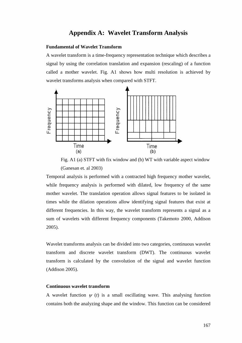
167
Appendix A: Wavelet Transform Analysis
Fundamental of Wavelet Transform
A wavelet transform is a time-frequency representation technique which describes a
signal by using the correlation translation and expansion (rescaling) of a function
called a mother wavelet. Fig. A1 shows how multi resolution is achieved by
wavelet transforms analysis when compared with STFT.
Fig. A1 (a) STFT with fix window and (b) WT with variable aspect window
(Ganesan et. al 2003)
Temporal analysis is performed with a contracted high frequency mother wavelet,
while frequency analysis is performed with dilated, low frequency of the same
mother wavelet. The translation operation allows signal features to be isolated in
times while the dilation operations allow identifying signal features that exist at
different frequencies. In this way, the wavelet transform represents a signal as a
sum of wavelets with different frequency components (Takemoto 2000, Addison
2005).
Wavelet transforms analysis can be divided into two categories, continuous wavelet
transform and discrete wavelet transform (DWT). The continuous wavelet
transform is calculated by the convolution of the signal and wavelet function
(Addison 2005).
Continuous wavelet transform
A wavelet function (t) is a small oscillating wave. This analysing function
contains both the analyzing shape and the window. This function can be considered
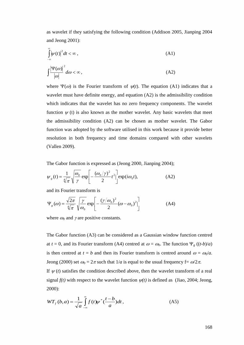
168
as wavelet if they satisfying the following condition (Addison 2005, Jianping 2004
and Jeong 2001):
dtt2
)( , (A1)
d
2)(
, (A2)
where () is the Fourier transform of (t). The equation (A1) indicates that a
wavelet must have definite energy, and equation (A2) is the admissibility condition
which indicates that the wavelet has no zero frequency components. The wavelet
function (t) is also known as the mother wavelet. Any basic wavelets that meet
the admissibility condition (A2) can be chosen as mother wavelet. The Gabor
function was adopted by the software utilised in this work because it provide better
resolution in both frequency and time domains compared with other wavelets
(Vallen 2009).
The Gabor function is expressed as (Jeong 2000, Jianping 2004);
),exp(2
)(exp
1)( 0
2
2
00
4tittg
(A2)
and its Fourier transform is
2
0
2
0
04
)(2
)(exp
2)(
g (A4)
where 0 and are positive constants.
The Gabor function (A3) can be considered as a Gaussian window function centred
at t = 0, and its Fourier transform (A4) centred at = 0. The function g ((t-b)/a)
is then centred at t = b and then its Fourier transform is centred around = 0/a.
Jeong (2000) set 0 = 2 such that 1/a is equal to the usual frequency f= /2.
If (t) satisfies the condition described above, then the wavelet transform of a real
signal f(t) with respect to the wavelet function (t) is defined as (Jiao, 2004; Jeong,
2000):
dta
bttf
aabWT f )()(
1),( *
, (A5)
169
where * denotes the complex conjugate of , and this is defined on the open (a, b)
half plane( a>0 and bR ). Parameters a and b stand for rescale and shift of the
basic wavelet function.
The analysis function for WT can be defined as
)()( 2
1
,a
btatba
, (A6)
which mean that every wavelet is generated by shifting and rescaling a basic
wavelet (t).
,)()(*)(),( dttfttabWT
(A7)
when function (t) satisfies the admissibility condition (A2), the original signal f(t)
can be obtained from the wavelet transform WT(b,a) by performing wavelet
inversion.
Discrete wavelet transforms (DWT)
The discrete wavelet transform and its inverse transform are defined as follows
(Addison, 2005):
dttftWT nmnm )()(* ,, , (A8)
),()( ,, tWTtf nm
m n
nm (A9)
where is a constant value for normalisations.
In the discrete domain, the scale and shift parameters are generally discretised as
a= a0m
and b= nb0 and the analysing wavelets are also discretised as follows:
),()(0
020, m
m
nma
nbtat
(A10)
where m and n are integer values.
Wavelet Coefficient
Wavelet analysis is fundamentally a correlation method. The wavelet coefficient,
c (t), provides information about the structure of input signal, f (t), and its
relationship to the shape of the analyzing wavelet, (t). The wavelet coefficient is
defined by the following correlation (Park, 2001):
170
dttttftc )'(*)'()(
(A11)
Where *(t) is the complex conjugate of (t) (pair of complex number, both
having a same real part, but with imaginary parts of equal magnitude and opposite
sign). When f (t’) correlate well with *(t’-t), c (t) will be large, but when they do
not correlate, c (t) will be small. Any wave shape may be used for the wavelet if it
is localised at particular time (Park, 2001).
Gabor Wavelet Gabor wavelet has been used in the analysis of AE signals due to its good
resolution in both time and frequency domain. The frequency component in the
output signal has been extracted from the output of the envelope of WT (Jeong
2001, Jingpin 2008):
21
)22cos(1)(2),( bkxaatxWT cgu (A 12)
Where WTu(x,t) is the magnitude of WT of signal x, g() is the Fourier
transform of the basic wavelet, the parameters a and b stand for scale and shift of
the basic wavelet, k is the wave number corresponding to frequency . The
magnitude of WT takes it maximum value at a = 0/c and b = (k/)x= x/cg. In
other words, the location of the peak on the (a,b) plane indicates the arrival time of
the group velocity cg at frequency c = 0/a, i.e., f = 1/a.
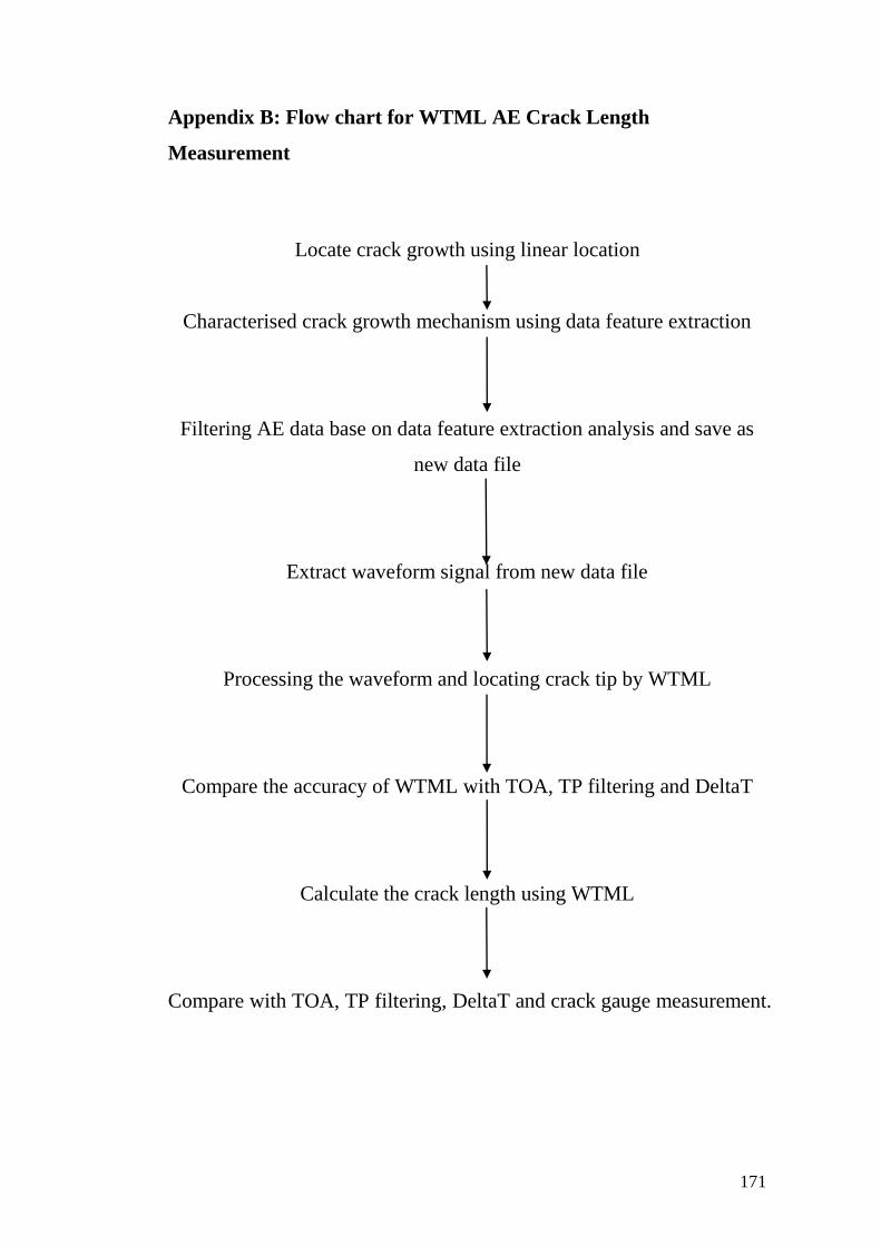
171
Appendix B: Flow chart for WTML AE Crack Length
Measurement
Locate crack growth using linear location
Characterised crack growth mechanism using data feature extraction
Filtering AE data base on data feature extraction analysis and save as
new data file
Extract waveform signal from new data file
Processing the waveform and locating crack tip by WTML
Compare the accuracy of WTML with TOA, TP filtering and DeltaT
Calculate the crack length using WTML
Compare with TOA, TP filtering, DeltaT and crack gauge measurement.