Acid Battery/Fuel Cell Hybrid Power

Automotive Research Center

A U.S. Army Center of Excellence for Modeling and Simulation of Ground Vehicles

Led by the University of Michigan

Control of a Lead-‐Acid Battery/Fuel Cell Hybrid Power System for a UGV: Experimental Report

Funded by:

U.S. Army Research Development and Engineering Command (RDECOM)

U.S. Army Tank Automotive Research, Development and Engineering Center (TARDEC)

In accordance with Cooperative Agreement W56HZV-‐14-‐2-‐0001

John A Broderick

Dawn M Tilbury

Ella M Atkins

December 2014

UNCLASSIFIED: Distribution Statement A. Approved for public release.

Control of a Lead-Acid Battery/Fuel Cell Hybrid Power System for

a UGV: Experimental Report

John A Broderick, Dawn M Tilbury, and Ella M Atkins

December 19, 2014

1 Introduction

Future robotic vehicles including both small unmanned ground vehicles (UGVs) and full-scale vehi-cles will carry multiple sources of power, including batteries, fuel cells, combustion engines, ultraca-pacitors, and/or solar cells, to allow for long-endurance operation. Fuel-based power sources havea higher specific energy than batteries, the reason most current automobiles are gasoline-powered.Batteries have other advantages, such as low noise profile, easy replacement, and direct energyconversion. Solar energy harvesting exploits natural resources to increase total energy reserves.Long-term missions, especially for autonomous robots that can operate indefinitely without humancontact, will require power systems operated together at maximum system efficiency. Ongoingresearch in the Automotive Research Center (ARC) looks at integration of multiple power sourcesfor ground robots together to increase energy efficiency and mission duration.

As part of the proposed work for ARC project 1.13: Reconfigurable Control for Energy andThermal Management in Unmanned Vehicles, hardware tests were conducted at TARDEC in theGround Systems Power and Energy Laboratory (GSPEL) to validate the models and methodologythat had been developed for optimization of multiple power sources. For these tests, the powersystem consists of an AMI 200 W solid oxide fuel cell and a TALON lead-acid battery pack; thisfuel cell was designed to power small ground robots and is easily mountable on a TALON. Thegoals of these tests were twofold: verify that average power provides sufficient information foroptimization purposes and demonstrate effectiveness of optimization compared to baseline controlscheme. Details of the optimization are presented in [3].

This report is organized as follows. Related work and an overview of the optimization method ispresented in Section 2. Section 3 details the hardware system used. Section 4 details the modelingof the TALON battery pack for use in the optimization. Battery Performance under averaged andvariable power demands is summarized in Section 5 and validation of the optimization routine ispresented in Section 6. Conclusions and Lessons Learned are presented in Section 7.

2 Background and Scope of Experiments

2.1 Related work

While current UGVs are almost universally battery powered, new research is looking at replacingor augmenting the battery with a fuel cell. Wilhelm et al. present a UGV powered exclusivelyby a fuel cell [11]. Their robot was quite small, using a 10 W fuel cell, and served as a proof ofconcept. Joh et al. present a humanoid robot powered by a fuel cell and a battery in parallel [6].The authors demonstrate the use of their robot, including the use of the battery to supplement the

1

fuel cell when the power demand exceeds the capacity of the fuel cell. However, the fuel cell is ableto vary the power output and there is no discussion of charging the battery when power demandsare low.

Hybrid power sources are a major area of interest in the automotive industry [5]. Most of thework is based on a combustion engine/battery hybrid. However, there are some initial investigationsinto a fuel cell/battery hybrid automobile [10]. Ceraolo et al. presents a general approach tohybrid power architectures for automobiles [4]. For cars, due to the fact that the engine producesmechanical power and the battery produces electrical power, one of the key design decisions isbetween a parallel, series, or more complex power connection. Optimization for these differentconfigurations have been studied (see [1, 7], for example).

More recently, Murphey et al. presented a power management scheme for a vehicle with multiplepower sources [8]. Each individual source can be turned on or off, in addition to any throttlingallowed by the device. Using a machine learning algorithm, the controller can decide at each timestep which power sources are the best to use. While this algorithm has the same purpose as ouralgorithm, there are several key differences. First, their model assumes that the power sourcescan be turned on and off instantaneously and, second, their optimization looks over a short timehorizon and not over an entire mission.

2.2 Optimization Method

To increase the mission life of a small ground robot, we have proposed a hybrid power modelingframework to control the power system by selecting which power sources to use [3]. Due to thelong transients in startup/shutdown of the fuel cell under consideration, we consider power systemuse over an entire mission. To solve this problem, we simplify the models to a form where theoptimization of the entire mission can take place in a short amount of time. This involves onlyusing the average power of the mission and averaging the dynamics of the different power systemsto meet the required simplifications.

Previously, we had considered a power system consisting of the 200 W fuel cell and a BB2590Li-ion battery pack [3]. We used an existing model of the battery to run the optimization andschedule fuel cell on/off times for a long-duration mission. Figure 1 compares the simplified modelto the full nonlinear model for the optimal schedule of fuel cell operation. For this power systemsimulation, the simplifications do not introduce significant errors.

To compare the effectiveness of our optimization algorithm, we also propose a simple controllerbased on the battery state of charge (SOC). The fuel cell is turned on (off) when the SOC reachesa low (high) threshold. These thresholds are chosen conservatively so that the battery is neverdepleted before the fuel cell is turned on while there is a 200 W load on the system and the entirepower output from the fuel cell can be used to charge the battery. Figure 2 shows the total energyusage over a mission using the optimization and this conservative control scheme. The optimizationscheme uses about 10% less power over the course of the entire mission.

2.3 Scope of Work

Having developed and compared this optimization in simulation, the next step is to validate themodels and assumptions used in a hardware setting. There are two main goals in these tests: confirmthat battery performance using an averaged power demand is sufficiently similar to performanceunder variable power demands and validate the optimization model against the real system.

While the simulation results are based on the BB2590 battery pack, due to incompatibilitiesbetween the fuel cell and the battery pack, a TALON lead-acid battery pack is used for the tests.

2

0 100 200 300 400 500 6000

10

20

30

40

50

60

70

80

90

Simple model

Full battery model

Variable Power

Figure 1: Comparing optimization model withfull system model

0 100 200 300 400 500 6000

1

2

3

4x 10

6

time [m]

Tota

l E

nerg

y U

sed [J]

SOC limits

Optimal

Figure 2: Comparing energy usage betweenbaseline controller and optimal scheduling

This requires that a model of the lead-acid battery be developed and integrated into the optimiza-tion routine in place of the BB2590 model. This model, along with all the experience and dataacquired from setting up and running the experience, are beneficial for future TARDEC projectslooking at powering the TALON with the fuel cell.

3 Hardware Setup

This section details the experimental setup for the fuel cell/battery hybrid power system. Usingthe fuel cell in parallel with the TALON battery kit and the data logger designed by the GSPELFuel Cell Lab, the battery and fuel cell currents and system voltages can be measured. The loadbank can be controlled to follow any given power profile. This setup allows for the load bank toemulate a robot power demand and to measure the power produced by the fuel cell and batteryduring system operation.

3.1 Ultra Electronics AMI Fuel Cell

(a) Fuel Cell (b) Propane Setup

Figure 3: AMI fuel cell with fuel tanks

The Ultra Electronics AMI Fuel Cell undertest is a 200 W propane solid oxide fuelcell. The fuel cell can be turned off andon by the small button on top of the fuelcell or by connecting to an external laptop.The connection is made through the smallheadphone jack on the top of the fuel celland a USB-serial converter connected tothe laptop. AMI has provided a LabVIEWexecutable to control the device.

The propane canisters are connected tothe fuel cell through a propane filter. Thetanks are positioned on a scale to measurethe current amount of fuel. The propane

3

tanks plus connectors weigh about 5.6 lbs when full and about 3.5 lbs when empty, though thesevalues are dependent on the arrangement of the system. The tanks and scale were on the bottomshelf of the cart and the filter and fuel cell on the top of the cart.

3.2 TALON Battery

The fuel cell is designed to work with the TALON lead acid battery pack. This pack consists of 3motorcycle batteries in series to produce the required voltage. The battery is B.B. Battery HR9-12.Each battery has a capacity of 8 Ah and 288 Wh and, combined in series, produce 36 V.

3.3 BK Precision Load Bank

Figure 4: Load Bank

The load bank used is a BK Precision 8510. The loadbank can be controlled manually or through a serial in-terface. LabVIEW modules are provided to initiate theserial communication and control system operation. Onlytwo modes of operation were used: constant current (forlogger calibration) and constant power. There are alsoconstant voltage and and constant resistance modes. Foreach mode of operation, the constant parameter (i.e. cur-rent for constant current) can be specified. The load bankrequires a ttl input for serial communication. This setupused a ttl/USB converter to connect to the external lap-top. The power input connects to the input terminals on the front of the device.

3.4 Data Logger

Hi there

Figure 5: Battery and Logger

The data logger for this system was designed by theGSPEL fuel cell lab. This logger consists of 2 batteryconnectors (on the same side), a fuel cell connector, anda load connector. The logger has an 8 pin header thatoutputs data voltages. With pin 1 closest to the loadconnector, the pins are as follows:

Pin Description1 Battery Current Sensor Output2 Fuel Cell Current Sensor Output3 Stepped-down System Voltage4 External Input5 External Input enabled6 Unconnected7 Unconnected8 Ground

The logger does not record these data fields. Instead,we connected the relevant pins to an NI-9205 Data Ac-quisition Unit housed in a NI-cDAQ. Using LabVIEW,the sampled data from the logger is read from the DAQand scaled to the actual values. To calibrate the differentfields, the following procedures were used.

4

Voltage The system voltage is stepped-down through a resistor network to about 10% of the realvalue. By comparing the voltage readings at the load bank for a 0 W command, the systemvoltage output is 10% of the actual voltage.

Current Sensor The data logger has 2 ACS756 current sensors, measuring the battery and fuelcell current individually. The current sensor output voltage scales linearly with the measuredcurrent. The 2 important calibrations are the bias and scale. The bias is the output voltagewhen zero current is measured. Nominally, the bias is half the VCC applied to the sensor(about 5 V in this setup). The bias can be easily measured by setting the load to 0 Wand measuring the output voltage. The scale is how much the voltage changes per ampof measured current (in the sensor documentation, the term sensitivity gives how much thevoltage changes per amp). Nominally, the scale is 25 A/V. To calibrate the scale, after settingthe bias, set the load bank to draw a constant current. With the known current the scale canbe calculated.

The logger was modified to have an external power supply instead of a 9V battery. The batterycan be reconnected by removing the top cover and loosening the board. On the backside, theexternal power supply wires can be disconnected and the battery carriage reconnected.

3.5 LabVIEW

The external laptop interfaces with the different components using LabVIEW. The basic outline ofthe program is to initialize communication, initialize power command data from file, record dataoutputs and send power commands for the duration of the test, then close communications. Thereare different loops for communication with each device and these loops end when the final timeis reached, the stop button is pushed, or there is an error in any communication stream. Whilethe communication loops occur asynchronously, all recorded data is marked with a synchronizedmeasurement time.

A new output folder based on the current time is created and 6 files are made: system parameter(mainly current sensor calibration values), power command, load bank measurement, fuel weightmeasurements, battery state of charge measurements and data logger measurements. Each is in csvfile format, with a row for each time step. The power command has the following columns: time,command. The fuel weight file has the following columns: time and weight. The SOC file has thefollowing measurements: time, measured SOC (based on integrating current), and estimated SOC(values are meaningless and never tuned). The load bank file has the following columns: time,voltage, current, power. The data logger file has the following columns: voltage, battery current,fuel cell current. This data is logged at a constant sample rate that is set on the main panel. Inthese tests, we mostly used 100 Hz.

The power command input file is formatted the same as the output file and the commandis linearly interpolated based on the current time and the closest two command points. Thecommunication blocks for the load bank include a 200 ms delay, so the power command is onlyupdated every 200 ms.

4 Battery Modeling

Due to the change in battery types between the simulation and the hardware tests, one of the firsttasks was to determine a battery model that could be used in the optimization. This was done bytuning a lead-acid battery model used by ARC project 1.10 to the batteries used in our setup [9].

5

0 100 200 300 400 50026

28

30

32

34

36

38

40

time [m]

Voltage

(a) Voltage over time, showing rapid discharges fol-lowed by voltage relaxation

0 100 200 300 400 500−1

0

1

2

3

4

5

6

time [m]

Voltage

(b) Repetitive current profile

Figure 6: Example pulse-relaxation test

02040608010032

34

36

38

40

42

SOC [%]

OC

V [

V]

Figure 7: OCV as a function of SOC

There are two main steps to finding the battery model: finding the open circuit voltage (OCV)as a function of state of charge and fitting the resistance/capacitance values to match the batteryperformance.

4.1 Pulse-Relaxation tests

To find the OCV, we use a pulse-relaxation test. The battery was initially charged and then aconstant current was drawn from the battery for a set time. The SOC is computed by integratingthe current draw. The battery is allowed to rest for a period of time while the voltage rebounds.The OCV is measured once the voltage has stabilized and the process is repeated. Figure 6 showsthe voltage and current profiles for one such test. From this test, the resulting OCV data is shownin Figure 7.

Table 1: OVC values for different SOC

SOC (%) 100.0 97.5 95.0 92.4 89.9 87.4 84.9 82.4 79.9 77.4 74.8 72.4 69.8OCV (V) 40.2 39.5 39.3 39.1 38.9 38.8 38.6 38.5 38.4 38.3 38.2 38.0 37.9

SOC (%) 67.3 64.8 62.3 59.8 57.3 54.8 52.3 49.8 47.3 44.8 42.3 39.8 37.3OCV (V) 37.8 37.6 37.5 37.4 37.3 37.1 37.0 36.9 36.7 36.6 36.5 36.3 36.2

SOC (%) 34.8 32.3 29.8 27.3 24.8 22.3 19.8 17.3 14.8 12.3 9.8 7.3 4.9OCV (V) 36.0 35.9 35.8 35.6 35.5 35.3 35.1 35.0 34.8 34.6 34.4 34.1 33.8

6

0 10 20 30 40 50 6035

36

37

38

39

40

41

time [m]

Ba

tte

ry V

olta

ge

Discharge− 150 W, optx−3

Simulation

Measured

0 20 40 60 80 10035

36

37

38

39

40

41

time [m]

Battery

Voltage

Discharge− Cov, optx−3

Simulation

Measured

Figure 8: Comparing battery model and measured voltage for two different power demands

0 50 100 15037.5

38

38.5

39

39.5

40

40.5

41

41.5

42

42.5

time [m]

Battery

Voltage

Simulation

Measured

0 20 40 60 80 100 12034

35

36

37

38

39

40

41

42

time [m]

Battery

Voltage

Simulation

Measured

Figure 9: Comparing battery model and measured voltage while charging

4.2 Battery model

The OCV-R-RC battery model from [9] presumes an OCV source in series with a resistor andan RC circuit. With the OCV known, the other parameters of the model must be found. Theprimary resistance R is parameterized by soc s as R = as2 + bs+ c. The RC circuit parameters areassumed to be constant over all SOC values. The quality of our curve fit was determined by thesquared difference between the simulated voltage and the measured voltage. Different parameterswere found for charging and discharging.

A series of experiments were conducted to tune the battery parameters, including pulse-relaxand discharge/charge tests. The parameters varied slightly between the different tests. Figures 8and 9 compare the battery simulation and the experimental measurements for the discharge andcharge profiles respectively. Model parameters were chosen by averaging the best fit parametersfor the different test cases. In the discharge tests, there is an interesting rebound in the measuredvoltage at the beginning of the test, which is not accounted for in the simulation model. Thisrebound is possibly due to battery heating. It is unclear if this is a common phenomenon in lead-acid batteries; however, it is very common in our tests. The tail portion of the simulation matches

7

0 200 400 600 800 1000 1200 140028

29

30

31

32

33

34

35

36

37

t [s]

Voltage [V

]

Data logger

Load Bank

(a) Voltage

0 200 400 600 800 1000 1200 1400

0.2

0.25

0.3

0.35

0.4

0.45

0.5

t [s]

SO

C

(b) State of charge

Figure 10: Battery reaches cutoff voltage before depletion

the experimental results quite well. For the charging case, the model matches the acquired dataclosely.

4.3 Other Battery Considerations

For power system optimization, the other key components of the model are the low SOC cutoff andthe charging characteristics. The SOC thresholds for the baseline control scheme depend on thesebattery parameters.

In one test shown in Figure 10, the battery voltage reached the lower voltage cutoff of 29 Vat about 18% state of charge. The voltage at the load bank is slightly lower then the data loggerdue to resistance in the wires between the logger and the load bank. The power demand for thistest was a constant 230 W. As such, we define the low limit on the state of charge as 18% for ourmodel. For optimization, we also introduce a safety margin to prevent the battery voltage fromgetting too close to the lower SOC limit.

0 0.2 0.4 0.6 0.8 1−6

−5

−4

−3

−2

−1

0

1

SOC

Curr

ent [A

]

Figure 11: Current ChargingProfile for Lead-Acid Battery

To determine charging characteristics of the combined fuelcell/battery system, the fuel cell was started with the battery ata lower state of charge and the battery was allowed to charge untilfull. As the battery charges, the system voltage increases until thevoltage converters in the fuel cell reach an upper limit. At thispoint the charging current decreases as the battery state of charge(and OCV) continues to increase. From experimental data, we pullout the charging curve, shown in Figure 11. The curve is fairlypiecewise-linear; at low SOC, the charging rate is constant basedon the maximum current available for the power output of the fuelcell above the mission demand. In this setup, this current matchesthe maximum charging current from the battery specifications. Once the battery reaches an SOCthreshold, the charging current decreases at a linear rate.

8

4.4 Variation Between Batteries

0 10 20 30 40 50 60 7020

25

30

35

40

time [m]

Battery

voltage [V

]

Old Battery 1

Old Battery 2

New Battery 1

Figure 12: Comparing Battery Performance

Each individual battery will have different per-formance. A total of four different batterieswere used during the summer tests. Two of thebatteries were older and had been used quitea bit with the TALON. As such, their operat-ing characteristics were quite degraded. Theother two batteries, which were the ones usedfor all the tests described above, were new andhad nearly identical behavior. As shown in Fig-ure 12, the new battery lasts longer than eitherof the old batteries, particularly old battery 2.While old battery 1 lasted close to the sametime as the new battery, the difference was greatenough to affect the battery model used in the optimization. This also shows how much the systemmodel might change over the life a component; a model that fits well for a new device would needto be adjusted as the device ages.

5 Battery Performance Under Different Power Demands

The first tests look at comparing battery performance under averaged and time varying powerdemands. One of the main assumptions in our optimization algorithm is that the averaged powerdemand is a valid approximation of time varying power demand. The simulation models suggestedthis approximation was valid; the purpose of these tests was to verify that assumption in hardware.

90 90.5 91 91.5 9220

40

60

80

100

120

140

160

180

200

time [m]

Po

we

r [W

]

Coverage Power Demand

Low Bandwidth Variability

High Bandwidth Variability

Average Power

Figure 13: Portion of power demands used in tests

Each test consists of operating the powersystem (battery and fuel cell) to meet a knownpower demand time history. The basic powerdemand for these tests is given by the areacoverage trajectory [3]. To prevent batterycharging currents from exceeding the maximumcharging current, a 30 W peripheral power de-mand is added. This power demand is con-sistent with constant power demands for thistype of robot [2]. The power demand, obtainedthrough simulation, is smooth; to add more re-alism, we also introduced different power loadswith more variation in the power demand overtime. Figure 13 shows the different power de-mand profiles. The variability is a random gaus-sian sample with the variance taken from testsdescribed in [2]. The “Low Bandwidth Variabil-ity” power demand has variability added every 3 seconds and the “High Bandwidth Variability”power demand has variability added every 0.2 seconds.

Four sets of tests were run. Each set was run on the same battery for repeatability. The first setwas completed with more variability in the initial battery state of charge, prompting the subsequentsets of tests. The second set of tests were run on a different battery and gave conflicting results,prompting the third set on the same battery. The fourth set of tests were run on battery used in

9

Table 2: Amp-hour during charge and discharge

(a) Second set

Cov. Path Low Band. High Band. AvgerageDischarge 6.02 5.9276 6.88 6.83

Charge 3.65 3.87 4.31 4.88(b) Third set

Cov. Path Low Band. High Band. AvgerageDischarge 6.75 6.83 6.37 6.89

Charge 4.86 4.85 4.43 4.81

the first tests to compare battery performance.

5.1 Test Procedure

The tests were run using the following procedure. First, the battery was discharged to about 40%SOC (36.35 V open circuit). The battery was allowed to rest to make sure the desired voltagewas achieved. Next, the fuel cell was turned on and allowed to start up. During this time, thepower system was under no load and the battery output current was recorded. When the fuel cellstarted producing power, the test was started and the load bank began to draw power accordingto the desired power profile for the test. Due to the variability of the fuel cell startup time, thebattery was at slightly different levels of charge when the tests began. The battery was allowed tocharge until power input to battery averaged around 20 W. The fuel cell was shut off and the testcontinued until the battery reached the low cut off voltage.

5.2 Test results

The tests were divided into charging and discharging portions due to the fact that the fuel cell isshut off at different times. Without this division, the discharge portions of the test could not bereadily compared. In each case, we compared the battery voltage and current and the time requiredto charge/discharge the battery.

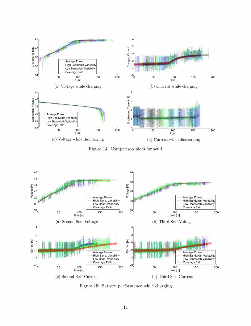
Figure 14 shows the results from the first set of tests. In these tests, the starting state of chargeof the battery was not as uniform at the beginning of the test. Because of this variability, the starttimes of the “High Bandwidth Variability” and “Low Bandwidth Variability” cases are shifted.This shift was determined manually to counteract the differences in starting state of the battery.After completing this test, a more thorough test procedure was devised to eliminate the need forthis manual adjustment.

In these tests, there is close agreement between the voltage and current over time during chargeand discharge phases. The total time for discharging the battery is also roughly equal between thedifferent tests. Compared to the “Average Power” case, the “Coverage Path” and “Low BandwidthVariability” tests take 2.7% and 0.5% longer respectively to discharge and the “High BandwidthVariability” takes 0.8% less time to discharge.

Figure 15 shows the voltage and current during charging for the second and third test sets. Inthe second set, there is some large differences between the current draws. The “Average Power”and “High Bandwidth Variability” tests have current draws that decrease linearly at the tail endof the charging cycle while the “Coverage Path” and “Low Bandwidth Variability” have closer toan exponential curve. In the third set, the current decreases linearly in all of the tests.

10

0 50 100 150 20034

36

38

40

42

t [m]

Charg

ing V

oltage

Average Power



Coverage Path

(a) Voltage while charging

0 50 100 150 200−6

−4

−2

0

2

4

t [m]

Charg

ing C

urr

ent

(b) Current while charging

0 50 100 150 20020

25

30

35

40

45

t [m]

Dis

charg

ing V

oltage

Average Power



Coverage Path

(c) Voltage while discharging

0 50 100 150 2000

2

4

6

8

t [m]

Dis

ch

arg

ing

Cu

rre

nt

[A]

(d) Current while discharging

Figure 14: Comparison plots for set 1

0 50 100 150 20037

38

39

40

41

42

43

time [m]

Vo

lta

ge

[V

]

Average Power

High Band. Variability

Low Band. Variability

Coverage Path

(a) Second Set- Voltage

0 50 100 150 20036

38

40

42

44

time [m]

Vo

lta

ge

[V

]

Average Power



Coverage Path

(b) Third Set- Voltage

0 50 100 150 200−6

−4

−2

0

2

4

time [m]

Cu

rre

nt

[A]

Average Power

High Band. Variability

Low Band. Variability

Coverage Path

(c) Second Set- Current

0 50 100 150 200−6

−4

−2

0

2

4

time [m]

Cu

rre

nt

[A]

Average Power



Coverage Path

(d) Third Set- Current

Figure 15: Battery performance while charging

11

0 20 40 60 80 100 120 14015

20

25

30

35

40

45

time [m]

Vo

lta

ge

[V

]

(a) Second Set

0 20 40 60 80 100 120 14025

30

35

40

45

time [m]

Vo

lta

ge

[V

]

(b) Third Set

Figure 16: Battery voltage while discharging

0 50 100 150 20037

38

39

40

41

42

time [m]

Vo

lta

ge

[V

]

Battery 2

Battery 1 (2)

Battery 1 (1)

(a) Coverage path

0 20 40 60 80 100 120 14025

30

35

40

45

time [m]

Vo

lta

ge

[V

]

(b) Average power demand

Figure 17: Comparing different batteries in same test

Figure 16 shows the data for the discharge portion of the same sets of tests. The second sethas significant variation, both in time to depletion and in the Amp-hour values in Table 2. It isunknown why this is. In contrast, the third set has close agreement between the different tests,with the exception of the high-bandwidth variability test. In particular, the battery is depletedfaster in the high-bandwidth variability than the other tests. The discharge time is 7.1% less thanthe “Average Power” test and uses 7.5% less current before full discharge, but has 7.9% less currentduring the charging phase, accounting for the discrepancy in discharge time. The difference in thehigh-bandwidth test is clearly visible. The “Coverage Path” power demand discharges the batteryin 0.66% less time and the “Low Bandwidth Variability” discharges the battery in 1.2% more timethan the average power case.

The forth set of tests were run to compare the two different batteries in use. Figure 17 comparesthe “Average Power” tests from the second, third, and forth sets of tests. There is close agreementbetween the different batteries. We cannot compare with the first set of tests because the powerdemand was 30 W lower in the first set.

6 Validation of Optimization

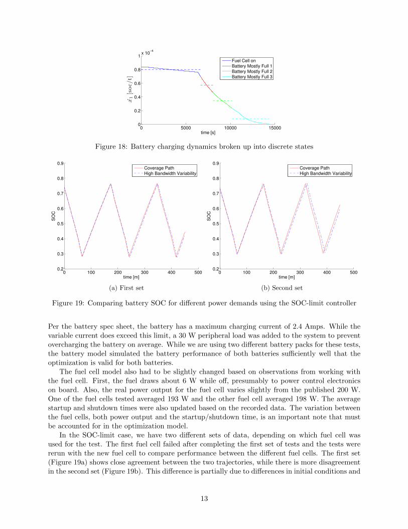
The first step of validating the optimization was to update the simulation battery model to includethe new lead-acid battery. For this, we used the model described in the Section 4. The mostimportant part is to determine the battery charging characteristics. Shown in Figure 18 is thebreakdown between the low charge and mostly charged states. This plot is very similar to thebreakdown for the BB2590 pack, though the drop off in charging is more linear than the BB2590.

12

0 5000 10000 150000

0.2

0.4

0.6

0.8

1x 10

−4

time [s]x1[soc/

t]

Fuel Cell on

Battery Mostly Full 1



Figure 18: Battery charging dynamics broken up into discrete states

0 100 200 300 400 5000.2

0.3

0.4

0.5

0.6

0.7

0.8

0.9

time [m]

SO

C

Coverage Path


(a) First set

0 100 200 300 400 5000.2

0.3

0.4

0.5

0.6

0.7

0.8

0.9

time [m]

SO

C

Coverage Path


(b) Second set

Figure 19: Comparing battery SOC for different power demands using the SOC-limit controller

Per the battery spec sheet, the battery has a maximum charging current of 2.4 Amps. While thevariable current does exceed this limit, a 30 W peripheral load was added to the system to preventovercharging the battery on average. While we are using two different battery packs for these tests,the battery model simulated the battery performance of both batteries sufficiently well that theoptimization is valid for both batteries.

The fuel cell model also had to be slightly changed based on observations from working withthe fuel cell. First, the fuel draws about 6 W while off, presumably to power control electronicson board. Also, the real power output for the fuel cell varies slightly from the published 200 W.One of the fuel cells tested averaged 193 W and the other fuel cell averaged 198 W. The averagestartup and shutdown times were also updated based on the recorded data. The variation betweenthe fuel cells, both power output and the startup/shutdown time, is an important note that mustbe accounted for in the optimization model.

In the SOC-limit case, we have two different sets of data, depending on which fuel cell wasused for the test. The first fuel cell failed after completing the first set of tests and the tests werererun with the new fuel cell to compare performance between the different fuel cells. The first set(Figure 19a) shows close agreement between the two trajectories, while there is more disagreementin the second set (Figure 19b). This difference is partially due to differences in initial conditions and

13

0 100 200 300 400 5000.2

0.3

0.4

0.5

0.6

0.7

0.8

0.9

1

time [m]

SO

C

Exp.− Coverage Path

Exp.− High BW Variability

Exp.− Slow Offsets

Simulation

Figure 20: Comparing Actual battery SOC withoptimization model

0 100 200 300 400 5000

1

2

3

4x 10

6

time [m]

Energ

y U

sed [J]

SOC−limits

Optimization

Figure 21: Energy usage for the SOC-limits andoptimization tests (Solid line- cov. power de-mand, dashed line- high band. variability powerdemand

a experimental error resulting in a slightly delayed (about 30 s) fuel cell restart. Due to differentfuel cell outputs, the data between fuel cells cannot be compared, however.

Figure 20 shows similar close agreement for the same tests using the optimization controller.There is close agreement between the optimization model and the experimental tests. This supportsour use of the approximation in the optimization routine.

Figure 21 compares the energy used over the course of the mission. To compute energy usage, weuse the weight of fuel consumed, scaled by the energy density of propane and the thermal efficiencyof the fuel cell, and the change in energy storage in the battery. The energy remaining in thebattery for a given SOC is calculated using the battery model. Using the unscaled propane energywould change the scale of the plot would be changed dramatically and hide what the optimizationis doing. This plot agrees closely with Figure 2 from simulation. This plot was determined usingactual fuel consumption and battery SOC, while the simulation plots were calculated by integratingthe power outputs from the battery and the fuel cell.

The optimization controller was run with an additional power demand. This power demand hada very low bandwidth variability in addition to the high bandwidth variability. In this case, a poweroffset was calculated for each 700 second portion of the trajectory. The average power demand forthis trajectory was the same as the average power for the baseline trajectory. This is similar to arobot that runs on constant terrain for a period, then on a different surface with slightly differentcharacteristics. Due to the large differences over time, the battery SOC is expected to deviate fromthe baseline test. This test was an experiment to see how far the averaging assumption can be taken.As shown in Figure 20, there is a large discrepancy over time due to the unexpected power demands.Additionally, the battery charging limits are encountered in the first charging cycle, leading to alower SOC at the end of the mission. This test shows the limits of the power demand assumptionused in the optimization. If the moving power average differs greatly from the overall average, thebattery can reach unsafe or inefficient operating conditions that the optimization routine cannotpredict. In this case, the power strategy would need to be adapted during the mission based onmeasured power usage. This adaptation is left for future work.

14

7 Conclusions and Lessons Learned

7.1 Conclusions

The results from these experiments confirm the assumptions that underpin the optimization routinethat was developed to maximize energy efficiency for a hybrid robot power system. In particular, weshowed that average and time varying power demands result in similar battery life and performance.The optimization routine is also able to conserve energy over the course of a mission and extendground robot performance.

These experiments also pointed out the sensitivity of the optimization algorithms on the powersystem components. When there is any variability in the components, whether startup times onthe same fuel cell or power output in different fuel cells, the optimization model can produceincorrect results. As such, a safety buffer must be added to the optimization to prevent the robotfrom running out of energy over the course of the mission. Future research needs to address thisdeficiency in the model.

7.2 Lessons Learned

Only two fuel cells were used during the tests this summer. One unit, labeled SYS0020R02N0022,was used for the majority of the tests before it began to fail during startup. The second unit, labeledSYS0020R02N0017, was used exclusively for the long duration tests (both SOC-limit control andoptimization).

The first major issue that occurred with the fuel cell was that it would occasionally turn offduring use. This was not a normal shutdown; it would be operating then immediately turn silentand the LabVIEW program would lose connection with the device. This occurred two or threetimes with the first fuel cell and once with the second fuel cell. After restarting the LabVIEWprogram, the fuel cell would be listed in the off state. The only anomalous reading that I could tellwas that the temperature sensors would show impossible data. One sensor would read 0 and theother would read 650 exactly. After a short time, the numbers would switch back to real values (inthe 600-700 range). Whenever this occurred, the fuel cell would be started up momentarily, thenshutdown before ignition began, allowing the fuel cell to enter the cool down state and return thedevice to a safe condition for restarting. The file “Data 140714 113814.txt” records the data fromthe fuel cell after the device was restarted. Unfortunately, the data logging was never turned onwhen the fuel cell shut down.

The other major issue with the fuel cell was that the first device started to fail on startup. Itonly occurred when the fuel cell was started soon after being shutdown. Sometimes the fuel cellwould pop as normal, but would take several minutes to get to that point, at which point it wouldimmediately fail.

For the first fuel cell, the startup time average about 820 seconds. One interesting point, whichmight be related to the failure described above, is that the fuel cell would take longer to start upon when it had recently been operating, taking closer to 900 seconds. The second fuel cell hada faster startup time, averaging about 740 seconds, though there were fewer startups to base thedata on. For this fuel cell, repeat startups took less time (about 40 seconds less).

The shutdown time is very consistent at 1000-1010 seconds for both fuel cells.

15

References

[1] Stefano Barsali, C. Miulli, and A. Possenti. A control strategy to minimize fuel consumptionof series hybrid electric vehicles. Energy Conversion, IEEE Transactions on, 19(1):187–195,2004.

[2] John A. Broderick, Dawn M. Tilbury, and Ella M. Atkins. Characterizing energy usageof a commercially available ground robot: Method and results. Journal of Field Robotics,31(3):441–454, 2014.

[3] John A Broderick, Dawn M Tilbury, and Ella M Atkins. Modeling and scheduling of multiplepower sources for a ground robot. In Proceedings of the ASME DSCC 2014, 2014.

[4] M. Ceraolo, A. Di Donato, and G. Franceschi. A general approach to energy optimization ofhybrid electric vehicles. Vehicular Technology, IEEE Transactions on, 57(3):1433–1441, 2008.

[5] C.C. Chan. The state of the art of electric, hybrid, and fuel cell vehicles. Proceedings of theIEEE, 95(4):704–718, 2007.

[6] Han-Ik Joh, Tae Jung Ha, Sang Youp Hwang, Jong-Ho Kim, Seung-Hoon Chae, Jae HyungCho, Joghee Prabhuram, Soo-Kil Kim, Tae-Hoon Lim, Baek-Kyu Cho, Jun-Ho Oh, Sang HeupMoon, and Heung Yong Ha. A direct methanol fuel cell system to power a humanoid robot.Journal of Power Sources, 195(1):293 – 298, 2010.

[7] Chan-Chiao Lin, Huei Peng, J.W. Grizzle, and Jun-Mo Kang. Power management strategy fora parallel hybrid electric truck. Control Systems Technology, IEEE Transactions on, 11(6):839–849, 2003.

[8] Yi L. Murphey, ZhiHang Chen, Leonidas Kiliaris, and M. Abul Masrur. Intelligent powermanagement in a vehicular system with multiple power sources. Journal of Power Sources,196(2):835 – 846, 2011.

[9] Yasha Parvini, Ernesto G. Urdaneta, Jason B Siegel, Saemin Choi, Ardalan Vahidi, and LeviThompson. Range extension study of a hybridized lead-acid battery using ultracapacitors viasimulation and experimental results from a 12 volt actively controlled hardware in the looptest bench. 2014. in preparation.

[10] P Rodatz, G Paganelli, A Sciarretta, and L Guzzella. Optimal power management of anexperimental fuel cell/supercapacitor-powered hybrid vehicle. Control Engineering Practice,13(1):41–53, 2005.

[11] Alexander N Wilhelm, Brian W Surgenor, and Jon G Pharoah. Design and evaluation of amicro-fuel-cell-based power system for a mobile robot. Mechatronics, IEEE/ASME Transac-tions on, 11(4):471–476, 2006.

16

Acid Battery/Fuel Cell Hybrid Power

Documents

Transcript of Acid Battery/Fuel Cell Hybrid Power