Achieving Performance Objectives for

Database Workloads

by

Anusha Mallampalli

A thesis

presented to the University of Waterloo

in fulfillment of the

thesis requirement for the degree of

Master of Mathematics

in

Computer Science

Waterloo, Ontario, Canada, 2010

©Anusha Mallampalli 2010

ii

AUTHOR'S DECLARATION

I hereby declare that I am the sole author of this thesis. This is a true copy of the thesis, including any

required final revisions, as accepted by my examiners.

I understand that my thesis may be made electronically available to the public.

iii

Abstract

In this thesis, our goal is to achieve customer-specified performance objectives for workloads in a

database management system (DBMS). Competing workloads in current DBMSs have detrimental

effects on performance. Differentiated levels of service become important to ensure that critical work

takes priority.

We design a feedback-based admission differentiation framework, which consists of three

components: workload classifier, workload monitor and adaptive admission controller. The adaptive

admission controller uses the workload management capabilities of IBM DB2’s Workload Manager

(WLM) to achieve the performance objectives of the most important workload by applying admission

control on the rest of the work, which is less important and may or may not have performance

objectives. The controller uses a feedback-based technique to automatically adjust the admission

control on the less important work to achieve performance objectives for the important workload. The

adaptive admission controller is implemented on an instance of DB2 to the test the effectiveness of

the controller.

iv

Acknowledgements

First, I would like to thank my supervisor Professor Kenneth Salem for his immense patience and

helpful advice. His continuous support not only helped me complete this thesis, but also helped me

stay optimistic through the low phases of life, when the progress was extremely slow. I also owe

many thanks to Keith McDonald at IBM Canada for his expert guidance with DB2 Workload

Manager (WLM) and his Database Workload Generator (DWG).

I would like to thank my readers Professor Ihab Ilyas and Professor Tim Brecht for helping me

significantly improve the quality of this thesis.

I am grateful to Paul Bird and Calisto Zuzarte for giving me an opportunity to spend a summer at

IBM Toronto Lab which not only led to this thesis work, but was also great fun. I would like to thank

Patrick Tayao, David Needs, Lee Johnson and Ahsan Khan for providing immediate support during

my initial frustrations with DB2 server issues and system issues.

I thank IBM Canada and Ontario Graduate Scholarship program for providing funding for this

research.

Finally, I would like to thank my family for supporting me, even if my decisions didn’t always

make sense to them.

v

Dedication

This is dedicated to my sister, Alekhya.

vi

Table of Contents

AUTHOR'S DECLARATION ............................................................................................................... ii

Abstract ................................................................................................................................................. iii

Acknowledgements ............................................................................................................................... iv

Dedication .............................................................................................................................................. v

Table of Contents .................................................................................................................................. vi

List of Figures ..................................................................................................................................... viii

List of Tables ........................................................................................................................................ ix

Chapter 1 Introduction ........................................................................................................................... 1

Chapter 2 Relevant Work ....................................................................................................................... 4

2.1 Load Control ................................................................................................................................ 5

2.2 Achieving Per-Class Performance Objectives ............................................................................. 7

2.2.1 Admission Differentiation ..................................................................................................... 8

2.3 Summary ...................................................................................................................................... 9

Chapter 3 Design and Implementation ................................................................................................. 11

3.1 Performance Objective Metric ................................................................................................... 11

3.2 Feedback-based Admission Differentiation Architectural Framework ..................................... 13

3.2.1 Framework Components ..................................................................................................... 13

3.3 Summary .................................................................................................................................... 22

Chapter 4 Experimental Evaluation ..................................................................................................... 23

4.1 Experimental Test Bed ............................................................................................................... 24

4.2 Database Workload Generator and Test Workloads .................................................................. 24

4.3 Experiment 1: Effect of WB on WA ............................................................................................ 27

4.4 Experiment 2: Effectiveness of Admission Control ................................................................... 28

4.5 Controller experiments with stable workload and fixed objective ............................................. 32

4.5.1 Controller Experiment 1: RS = 1082, KI = 0.01, I = 20 ....................................................... 33

4.5.2 Controller Experiment 2: RS = 1682ms, KI = 0.001, I = 40 ................................................ 36

4.5.3 Conclusion .......................................................................................................................... 38

4.6 Controller Experiments with Stable Workload and Changing Objective .................................. 38

4.6.1 Controller Experiment 3: RS = 1058ms -> 1082ms ............................................................. 38

4.6.2 Controller Experiment 4: RS = 1105ms -> 1058ms ............................................................ 41

4.6.3 Controller Experiment 5: RS = 1824ms -> 1058ms ............................................................ 43

vii

4.6.4 Conclusion ........................................................................................................................... 45

4.7 Controller Experiments with Changing Workloads and Fixed Objective .................................. 45

4.7.1 Controller Experiment 6: Workload increase ...................................................................... 46

4.7.2 Controller Experiment 7: Workload decrease ..................................................................... 49

4.7.3 Conclusion ........................................................................................................................... 52

4.8 Controller Parameter Tuning and Discussion ............................................................................. 52

4.8.1 Controller Experiment 8: Performance Problem with Small Controller Constant KI ......... 53

4.8.2 Controller Experiment 9: Performance Problem with Large Controller Constant KI ......... 55

4.8.3 Controller Experiment 10: Performance Problem with improper Control Interval I........... 57

4.8.4 Tuning Controller Constant KI and Control Interval I Experimentally ............................... 59

4.8.5 Choosing Controller Constant KI ........................................................................................ 59

4.8.6 Choosing Control interval I ................................................................................................. 63

4.9 Workloads with Small Inter-Arrival Time and Small Service Time .......................................... 63

4.9.1 Effectiveness of Controller on Workloads with Higher Arrival Rate ................................. 63

4.9.2 Effectiveness of Controller on Workloads with Small Service Time .................................. 65

4.10 Summary .................................................................................................................................. 66

Chapter 5 Conclusion ........................................................................................................................... 68

References ............................................................................................................................................ 71

viii

List of Figures

Figure 1: CPU-bound Query's Life ...................................................................................................... 12

Figure 2 Feedback-based Admission Differentiation Framework ....................................................... 14

Figure 3: Feedback control loop timeline and control interval I .......................................................... 18

Figure 4: Adaptive Admission Controller’s block diagram ................................................................. 22

Figure 5: Baseline is WA and WB when run in isolation. Problem instance is WA and WB when run

together. The bars show response time averages and error bars show standard deviations in the

response times. ..................................................................................................................................... 28

Figure 6: Sensitivity to concurrency threshold on WB. (a) shows response time average of WA for

each concurrency threshold on WB. (b) shows throughput of WB for each concurrency threshold on

WB. Error bars indicate standard deviation in the measurements at each concurrency threshold. ....... 29

Figure 7: Controller experiment results with inputs RS = 1082ms, KI = 0.01, I = 20 .......................... 35

Figure 8: Controller experiment results with inputs: RS = 1682ms, KI = 0.001, I = 40 ....................... 37

Figure 9: Controller experiment results with inputs: RS = 1058ms->1082ms, KI = 0.01, I = 20 ......... 40

Figure 10: Controller experiment results with inputs: RS = 1105ms->1058ms, KI = 0.01, I = 20 ....... 42

Figure 11: Controller experiment results with inputs: RS = 1824ms->1058ms, KI = 0.01/6, I = 40 .... 44

Figure 12: Controller experiment results with inputs: RS = 1105ms, KI = 0.01/6, I = 20 .................... 48

Figure 13: Controller experiment results with inputs: RS = 1105ms, KI = 0.01/6, I = 20 .................... 51

Figure 14: Controller experiment results with inputs: RS = 1082ms, KI = 0.001, I = 20 ..................... 54

Figure 15: Controller experiment results with inputs: RS = 1682ms, KI = 0.01, I = 20 ....................... 56

Figure 16: Controller experiment results with inputs: RS = 1682ms, KI = 0.001, I = 20 ..................... 58

Figure 17: Sensitivity of response time average of WD to concurrency threshold on WE ................... 64

Figure 18: Sensitivity of response time average of WF to concurrency threshold values on WG ........ 66

ix

List of Tables

Table 1: Test workloads WA and WB configurations ........................................................................... 26

Table 2: Response time average and standard deviation of WA for each concurrency threshold C from

Figure 6(a) ............................................................................................................................................ 30

Table 3: RS is the response time objectives for WA used in the experiments and expected concurrency

threshold is the threshold value that is expected to be chosen by the controller. ................................. 32

Table 4: Test workload WC configuration ............................................................................................ 45

Table 5: Workloads in each phase of Experiment 6 ............................................................................. 46

Table 6: Workloads in each phase of Experiment 7 ............................................................................. 49

Table 7: Test workloads WD and WE configurations ............................................................................ 64

Table 8: Test workloads WF and WG configurations ............................................................................ 65

1

Chapter 1

Introduction

Database management systems (DBMS) must accommodate a variety of workloads, which come in

from different sources, and which may have different service-level objectives. Service-level

objectives may be time-based, such as a goal to keep the throughput or the response time of a

workload to be below a certain threshold, or may be hard to quantify, such as a goal to keep the users

of a database happy and to prevent any aberrant database activity from hampering their day-to-day

work [1]. Time-based objectives are a standard representation of the performance requirements of the

workloads and hence, are most commonly known as performance objectives. In essence, a

performance objective of a workload reflects the workload’s desired resource requirements.

In a resource constrained environment, achieving the performance objectives of all of the

workloads may be impossible. Differentiated levels of service become necessary. Our objective in

this thesis is to design a mechanism which ensures that the performance objectives for the most

important workload are met, while handling the rest of the work, which is less important and may or

may not have performance objectives, at the best level possible. For example, if there is a large

amount of work from a less important application taking up most of the resources in a DBMS,

deteriorating the performance of a workload from an important application, we can throttle the less

important application just enough to achieve the performance objective of the important workload.

The idea is not to waste scarce system resources on less important work in a DBMS. From here on in

this thesis, we call the most important workload the primary workload and the other, less important

workload the secondary workload.

Admission control is a popular technique used for load control in DBMSs. The load of a workload

in a system can be regulated by controlling the workload’s admission level, defined as the number of

queries from that workload that are allowed to execute at any given time. Those queries that are not

admitted because the workload’s admission level has been reached are placed in a waiting queue so

that they can be processed at a later time. Therefore, we essentially work on service differentiation

through admission control, which we will call admission differentiation from here on, to achieve

performance objectives. In this thesis, we present an architectural framework that applies admission

control on the secondary workloads so that the primary workload can achieve its performance

2

objective. The framework not only uses admission differentiation to achieve performance objectives

for a primary workload, but also ensures best-effort service for the secondary workloads.

Admission control requires accurate calculation of the admission level for the secondary

workloads. If the admission level is too low, we end up delaying a lot of queries, resulting in an

underutilized system. If the admission level is too high, we end up admitting too many queries, which

might result in unfulfilled performance objectives. Therefore, we need an analytical method as

framework’s decisional underpinning.

Feedback-based techniques can provide an analytical foundation for achieving a performance

objective. They use the current performance of the primary workload as feedback to adjust the

amount of admission control on the secondary workloads. The amount by which the admission

control level should be adjusted is calculated by using control theory [2]. It enables our framework to

not only converge onto a performance objective value efficiently but also adapt to unpredictable

workload changes in the system. Hence, we call the framework feedback-based admission

differentiation.

This thesis makes two principal contributions:

An architectural framework for feedback-based admission differentiation (Chapter 3). The

framework achieves performance objectives of a primary workload on an instance of IBM

DB2. The framework includes a feedback-based control loop that adds to the existing

workload management capabilities in DB2’s Workload Manager [1]. In the feed-back control

loop, the current performance of the primary workload is measured and compared to its

objective, based on which the amount of control on the secondary workload is manipulated at

regular intervals.

An empirical evaluation of the admission controller mechanism (Chapter 4). We test the

mechanism in different scenarios, in which workloads and performance objectives are varied.

The rest of the thesis is structured as follows. Chapter 2 presents related work on admission control

and how it has been used to achieve various performance objectives. Chapter 3 presents an

architectural framework for feedback-based admission differentiation. We discuss the design and

implementation of the key functional components involved in the framework that work together to

achieve performance objectives for the primary workload by applying admission control on the

secondary workload. Chapter 4 presents a performance analysis of the mechanism. The thesis

3

concludes with an explanation of the lessons learned, suggestions for enhancements and future

research in this line of work for database management systems.

4

Chapter 2

Relevant Work

Current research in workload management concentrates on workload performance management.

Various methods for manipulating the performance of the workloads have been proposed. A query’s

life in a workload gives us three areas of scope for controlling performance of a workload. The first

opportunity is to decide whether a new query coming into the system is to be allowed to execute

immediately or not. Those that are not executed immediately might be delayed (queued) or rejected.

The second opportunity is to make scheduling decisions for the rejected queries. The third

opportunity is to control the execution of running queries [3]. These three opportunities have led to a

significant amount of work, resulting in three important types of resource control in workload

management: admission control [4-14], query scheduling [8, 9, 13, 15-17] and execution control [18-

21]. Since we use admission control as the resource control technique, we focus on the admission

control research.

Admission control has been traditionally used for OLTP workloads to prevent potential problem

queries from overloading the system. Admission control works by adjusting the multi-programming

level (MPL), which is the maximum number of queries that are permitted to run concurrently.

Unfortunately, choosing an MPL is not an easy task. If the MPL is set too high then it leads to

system overloading and if the MPL is set too low then it leads to system underutilization. Moreover,

with database systems having to operate in changing workload conditions, the MPL should be

adaptive. Therefore, it may be difficult for a human system administrator to tune the MPL manually.

A significant body of work exists on admission control in the form of various feedback-based

techniques to tune the MPL [4-14].

In the rest of this chapter, we present related work on admission control. In Section 2.1, we present

the work in which admission control was used to control the load of all the workloads running on a

system. They work on achieving global performance objectives. In Section 2.2, we present the work

in which admission control has been used to achieve per-class performance objectives.

5

2.1 Load Control

Most of the early work on feedback-based techniques in applying admission control has focused on

load control. These techniques aim at achieving an optimal MPL, which is high enough to maximize

the throughput of the workload in the system and low enough to avoid overloading and performance

degradation.

Monkeberg et al [4], Carey et al [5] and Heiss et al [6] focus on interactive transactional workloads.

Moenkeberg et al [4] measure a performance metric called conflict ratio, which is the ratio of the

number of locks held by all transactions to the number of locks held by active transactions. If the ratio

exceeds a critical threshold of 1.3, found experimentally, the admission of new transactions is

suspended, letting them queue. Otherwise one or more transactions waiting in the queue are admitted.

Similarly, Carey et al [5] measure the ratio of queued (blocked) transactions to running transactions.

If the ratio exceeds a threshold of 0.5, the admission of new transactions is suspended. Otherwise, one

or more transactions are admitted. The work done by Moenkeberg et al [4] and Carey et al [5] uses

static thresholds obtained through experiments to determine the amount of admission control to be

applied. These thresholds may be specific to the test system used to conduct the experiments.

Unlike Moenkeberg et al and Carey et al, Heiss et al [6] use a more general approach to calculating

the MPL in the system. They use two heuristic algorithms: incremental steps (IS) and parabolic

approximation (PA). In the IS algorithm, they start with an arbitrary value for the MPL and then they

increase the MPL by 1 at regular time intervals and measure transaction throughput. If the throughput

has increased, then they continue to increase the MPL, or if the throughput has decreased, then they

decrease the MPL at regular time intervals until the throughput starts to decrease again. In the PA

algorithm, they use a parabolic function to determine the new MPL. The parabolic function

approximates the performance in the system using the recent measurements of the performance for

different MPL values. The maximum of the parabolic function is used as the new MPL. Their

algorithm is restricted to parabolic performance functions and therefore the algorithm cannot be used

with performance metrics that do not follow parabolic functions such as query latencies or response

times which are often used to define service level objectives for workloads in current DBMSs. Their

goal is to maximize throughput in the system and hence, find the highest possible MPL for the whole

system that would prevent overloading. In contrast, our goal is to achieve performance objectives for

a primary workload and hence, find the best possible MPL on the secondary workload. We use

fundamentals from control theory for calculating the MPL on the secondary workload.

6

Kang et al [7] also use admission control to control the load. They pre-determine the CPU

utilization of a query and admit it only if its CPU utilization requirement is available in the system to

service it. Similarly, Elnikety et al [8] also use admission control to provide overload protection for

web servers by rejecting requests which would overload the server and placing them in a queue. Their

goal is to see to it that the current CPU utilization does not exceed the system’s capacity. In order to

admit a query, they pre-estimate the CPU utilization of the query. They add the estimate to the current

CPU utilization, which is also an aggregated estimate of the CPU utilizations of all the previously

admitted queries that are running in the system. If the sum is less than the system capacity, then query

is admitted. Therefore, effectively, they use estimates to admit a query. In contrast, our controller uses

the primary workload’s current, actual performance to understand the effect of load caused by the

secondary workload. Based on this feedback, the controller controls the CPU utilization of the

secondary workload by controlling the secondary workload’s MPL, which determines whether the

workload’s future, incoming queries can be admitted or not.

Schroeder [9] uses a combination of queuing theoretic models and feedback-based control to

determine the optimal MPL for the server. Her approach takes as inputs (from the DBA) the

maximum allowable thresholds for drop in throughput (from the highest throughput in the system)

and increase in response time (from the lowest response time in the system) and determines the

lowest optimal MPL. The queuing theoretic models are used to find a close-to-optimal MPL and then,

a feedback-based controller compares the current throughput and the current response time with their

respective thresholds. Based on these comparisons, the controller makes conservative adjustments to

the determined MPL. Similarly, Kang et al [10] also implement admission control by controlling the

MPL to control data contention. They measure the system’s data contention in the form of a data

contention ratio, which is the ratio of the number of locks held by all transactions (blocked and

active) to the number of locks held by active transactions. Their goal is to achieve a user-specified,

desired threshold for the data contention ratio. Based on the measured value of the data contention

ratio and the desired threshold, they use control theory to determine the amount by which the MPL is

to be tuned. Similarly, we also use fundamentals from control theory to determine the amount by

which the MPL is to be tuned. However, Kang, Sin and Shin concentrate only on data contention due

to locking involved between queries running in the system. Our controller approach differs in that our

framework works with workloads for which CPU contention is the problem. In addition, Kang et al

cancel admitted transactions that are blocked, waiting for locks, to alter the MPL in the database

server, but we do not cancel any admitted transactions.

7

As explained in the previous chapter, unlike all of the above work, we do not apply admission

control globally throughout the system to prevent overloads and we do not achieve global

performance objectives. Instead, we apply admission control on the secondary workloads alone to

regulate the CPU load caused by them just enough to achieve performance objectives for the primary

workload.

2.2 Achieving Per-Class Performance Objectives

There exists a fair amount of work on using admission control to achieve performance objectives for

individual workloads. The workloads are categorized into workload classes and each class is

monitored and controlled to achieve its performance objective.

Brown et al [11] were among the first to work on achieving performance objectives for workload

classes in a DBMS. They introduced an algorithm called M & M that uses memory allocation and

MPL to achieve response time objectives for workload classes. They classify queries into workload

classes according to their performance objectives. Then, they use a set of heuristics to determine the

MPL and the memory allocation for each workload class. The heuristics filter the search space of

possible solutions of combinations of the MPL and the memory allocation for a workload. These

heuristics underappreciate the interdependencies among the workloads. Workloads are dependent on

one another because they compete for shared resources. For example, if the MPL of a workload is

increased, this improves the performance of the workload, but it may result in increased response time

for the other workloads. Brown et al solve this dependency problem by incorporating performance

feedback along with their heuristics. They measure the response time of a class regularly after a

certain number of query completions and compare it to the objective. Based on the results of the

comparison, they tweak the MPL and the memory allocation settings. Our work is different from M &

M, because we don’t try to logically partition the available resources between various workload

classes to achieve their performance objectives by performing direct resource allocation. We try to

achieve performance objectives in an overloaded environment by sharing the available resources

among the workload classes. Our admission differentiation uses the interdependence of the workload

classes by using admission control on the secondary workloads to affect the performance of the

primary workload.

8

The M&M is devoid of any knowledge regarding the business importance of the workloads. Pang

et al [12] integrate the importance of the workloads into their MPL and memory settings. Pang et al

classify queries into workload classes based on their importance. Like M&M, the algorithm of Pang

et al achieve the response time objective of a class by measuring the response time of the class

regularly after a certain number of query completions and comparing it to the objective. The MPL is

based on this comparison. The MPL is calculated by using a statistical projection called the miss

ratio, which is the proportion of queries that fail to complete by their deadlines. If the statistical

projection fails, they use resource-utilization heuristics.

Apart from using admission control through MPL, Brown et al [11] and Pang et al [12] use direct

resource allocation by allocating memory for each workload class in order to achieve the class’s

performance objective. The advantage of using direct resource allocation is that a finer granularity

can be achieved in controlling the performance of a workload. However, a disadvantage of this

approach is that it requires changes to database internals and working at a level that requires operating

system support. Our approach is different in that we design and implement an admission control

mechanism that works at a level external to the database engine. The advantage of this approach is

that it does not depend on changes to the database internals, making portability easier, or knowledge

of the resource utilization of the workload, making implementation easier. Brown et al and Pang et al

also test their approach in a simulated environment without experimental validation on a DBMS.

2.2.1 Admission Differentiation

In current resource-constrained systems, if all workload classes are processed with the same level of

urgency, then the workloads can compete with each other for shared resources. This can be

detrimental on the performance of the system as a whole. Achieving performance objectives of all of

the workload classes may not be possible. One workload class has to be favoured over another

workload class. Therefore, the importance of the workload classes needs to be considered while

achieving their performance objectives.

The following is work done on the use of admission control to provide service differentiation in

web servers. Bhatti et al [13] perform a part of their service differentiation by performing admission

control on lower priority requests. Such requests are rejected when the number of higher priority

requests waiting in the execution queue exceeds a certain threshold, which is determined through

9

experimentation. Rejection is accomplished by closing the connection of the request. Like Bhatti et al,

we also apply admission control on secondary workloads to prevent our primary workload’s

performance from being affected due to overload in database management systems.

Similarly, Abdelzaher et al [14] also combine service differentiation with admission control. They

achieve a performance objective, capacity utilization, for a high-priority workload class by applying

admission control on a lower priority workload class to control the MPL. The lower priority requests

that will exceed the MPL are rejected. They use a combination of proportional and integral control to

determine the MPL by monitoring the current utilization and comparing it with the objective. Our

work in this thesis applies admission differentiation in the same way as Abdelzaher et al to workloads

in database management systems. We achieve response time objectives for the primary workload

through admission control in the form of controlling the MPL of the secondary workloads. We also

use fundamentals from control theory in our decision logic to determine the amount by which the

MPL has to be changed. However, their components that make up the controller require changes to

the server internals for implementation. Unlike Abdelzaher et al, we work outside the database engine

and therefore we do not touch the database internals.

2.3 Summary

In summary, there are three take away concepts from this chapter.

1. MPL control: All of the above work has implemented admission control by controlling the

MPL. Many kinds of performance objectives can be achieved by controlling the MPL. Our

algorithm also controls the MPL of the secondary workloads to achieve the performance

objectives of the primary workload.

2. Feedback-based control: All of the above work, except Kang et al [7] and Elnikety et al [8],

use monitoring as a part of their approach for admission control. They integrate monitored

information into decision making for calculation of the MPL value. We do the same by

monitoring the performance of the primary workload to determine the admission control to be

applied to the secondary workloads.

3. Decision logic: Most of the work done on admission control, either to provide overload

protection or to achieve a performance objective, uses predefined heuristics and simple

mathematical approaches in calculating the amount of admission control to be applied. Like

10

Kang et al [10] and Abdelzaher et al [14], we use fundamentals from control theory in our

decision making because they have been popularly used for working in dynamic scenarios.

11

Chapter 3

Design and Implementation

In this chapter, we present the design of an architectural framework for feedback-based admission

differentiation. Our high-level design goal is to adaptively achieve performance objectives for the

primary workload. If there are changes in the workloads or the performance objectives, the

framework’s components should work together to dynamically respond to changes without the

intervention of the database administrator and achieve performance objectives for the primary

workload. For implementing the framework, we use IBM DB2 as our database management system.

Before presenting the framework and its components, we present our performance objective

specification.

3.1 Performance Objective Metric

The most commonly used performance metrics for performance objectives are throughput [6, 9] and

response time [9, 11, 12]. Throughput is usually used for batch workloads. Batch workloads aim at

maximizing their utilization of the processor so that the workloads finish within a specified time

interval, known as the batch window. These workloads focus on executing as many queries as

possible and therefore, it suffices to focus on the number of transactions completed. Response time

objectives are commonly used for transactional workloads. For our implementation, we use CPU-

bound transactional workloads and therefore, we try to achieve response time objectives.

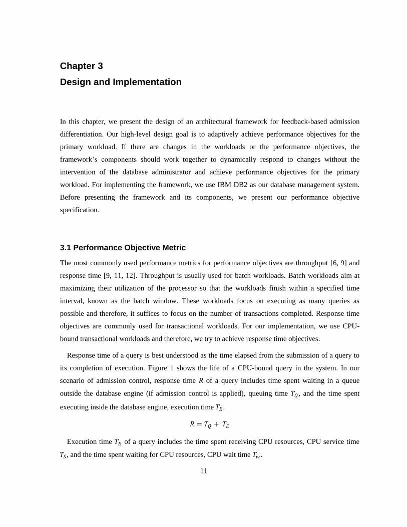
Response time of a query is best understood as the time elapsed from the submission of a query to

its completion of execution. Figure 1 shows the life of a CPU-bound query in the system. In our

scenario of admission control, response time R of a query includes time spent waiting in a queue

outside the database engine (if admission control is applied), queuing time 𝑇𝑄, and the time spent

executing inside the database engine, execution time 𝑇𝐸 .

𝑅 = 𝑇𝑄 + 𝑇𝐸

Execution time 𝑇𝐸 of a query includes the time spent receiving CPU resources, CPU service time

𝑇𝑆, and the time spent waiting for CPU resources, CPU wait time 𝑇𝑤 .

12

𝑇𝐸 = 𝑇𝑆 + 𝑇𝑤

Therefore,

𝑅 = 𝑇𝑄 + 𝑇𝑆 + 𝑇𝑤

Figure 1: CPU-bound Query's Life

In order to regulate the response time of a workload towards the workload’s performance objective,

the queuing time or the CPU service time or the CPU wait time of the queries of the workload should

be controlled. We do not apply admission control on the primary workload and therefore, there is no

queuing time 𝑇𝑄 for the primary workload. Service time 𝑇𝑆 is the inherent nature of a query and

therefore, cannot be changed. CPU wait time 𝑇𝑤 is mainly dependent on the CPU resource

contention. Hence, the focus of our framework narrows down to controlling the CPU wait time 𝑇𝑤 of

the primary workload by controlling the CPU contention in the system, which is done by applying

admission control on the secondary workload.

13

Response Time Objective Specification

In this thesis, we aim at achieving a response time objective for the primary workload. For example,

average response time of the workload should be 1000 ms.

3.2 Feedback-based Admission Differentiation Architectural Framework

In this section, we present the components required to perform feedback-based admission

differentiation and discuss the design and implementation of each component involved.

3.2.1 Framework Components

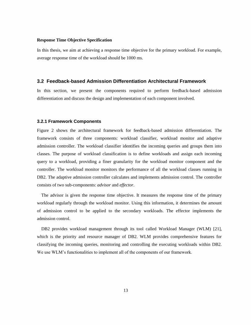
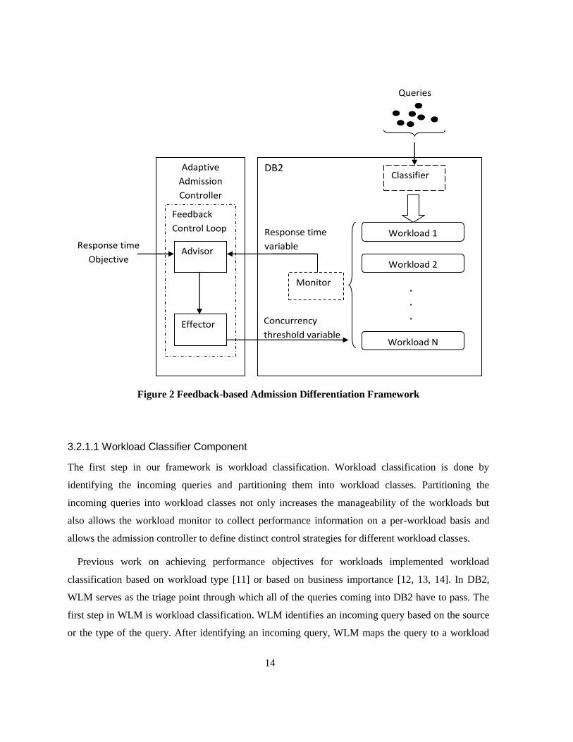
Figure 2 shows the architectural framework for feedback-based admission differentiation. The

framework consists of three components: workload classifier, workload monitor and adaptive

admission controller. The workload classifier identifies the incoming queries and groups them into

classes. The purpose of workload classification is to define workloads and assign each incoming

query to a workload, providing a finer granularity for the workload monitor component and the

controller. The workload monitor monitors the performance of all the workload classes running in

DB2. The adaptive admission controller calculates and implements admission control. The controller

consists of two sub-components: advisor and effector.

The advisor is given the response time objective. It measures the response time of the primary

workload regularly through the workload monitor. Using this information, it determines the amount

of admission control to be applied to the secondary workloads. The effector implements the

admission control.

DB2 provides workload management through its tool called Workload Manager (WLM) [21],

which is the priority and resource manager of DB2. WLM provides comprehensive features for

classifying the incoming queries, monitoring and controlling the executing workloads within DB2.

We use WLM’s functionalities to implement all of the components of our framework.

14

Queries

Adaptive

Admission

Controller

DB2

Workload 1

Feedback

Control Loop

Classifier

Workload 2

.

.

.

.

.

.

.

Workload N

Response time

Objective

Monitor

Concurrency

threshold variable

Response time

variable Advisor

Effector

Figure 2 Feedback-based Admission Differentiation Framework

3.2.1.1 Workload Classifier Component

The first step in our framework is workload classification. Workload classification is done by

identifying the incoming queries and partitioning them into workload classes. Partitioning the

incoming queries into workload classes not only increases the manageability of the workloads but

also allows the workload monitor to collect performance information on a per-workload basis and

allows the admission controller to define distinct control strategies for different workload classes.

Previous work on achieving performance objectives for workloads implemented workload

classification based on workload type [11] or based on business importance [12, 13, 14]. In DB2,

WLM serves as the triage point through which all of the queries coming into DB2 have to pass. The

first step in WLM is workload classification. WLM identifies an incoming query based on the source

or the type of the query. After identifying an incoming query, WLM maps the query to a workload

15

class and subsequently, maps all the other queries coming in from the same source or of the same type

to the same workload class.

In the implementation of our adaptive admission controller on DB2, for simplicity, we assume that

there are only two workload classes, primary and secondary. The workload classifier has to be

configured to identify the primary workload queries and group them into a primary workload class

and group all other incoming queries into a secondary workload class. Hence, each workload should

have its own individual workload class so that we can monitor each workload class individually and

control each workload class uniquely.

3.2.1.2 Workload Monitor Component

Workload monitor collects the performance information of the workloads. DB2’s WLM provides

various means of capturing performance information about individual workloads running on the

system. There are table functions that provide access to real-time information and event monitors to

capture detailed query information and aggregate information for historical analysis [21]. Statistics

from an event monitor can be read by resetting the statistics. Statistics can be reset by using a stored

procedure called WLM_COLLECT_STATS(), which sends the statistics to a set of tables and

histograms. The statistics can then be viewed by querying the statistics tables and viewing the

histograms. In contrast, table functions can be used to obtain point-in-time execution information

without having to reset statistics.

In the implementation of our adaptive admission controller, we focus on the response time

information of the primary workload. In order to understand whether the primary workload is meeting

its response time objective or not, we need to use an event monitor to capture response times

aggregated over a single control interval, after which the statistics need to be reset so that the next

control interval can be monitored. We use the event monitor DB2STATISTICS to collect aggregate

execution information. For obtaining response time information, WLM provides lifetime average and

execution time average in milliseconds. Lifetime average is the sum of queuing time average (due to

admission control by WLM) and execution time average. Execution time average is the sum of CPU

service time and CPU wait time. Therefore, in our implementation, if we want to measure the

response time average of the primary workload, we use execution time average and if we want to

16

measure the response time average of the secondary workload, we use lifetime average because it

includes queuing time due to admission control as well.

The response time average of the primary workload is read by querying for the execution time

average COORD_ACT_EXEC_TIME_AVG and the response time average of the secondary

workload is read by querying for the life time average COORD_ACT_LIFETIME_AVG from the

statistics table SCSTATS_DB2STATISTICS, where the event monitor’s aggregate statistics of all the

workloads are written to.

3.2.1.3 Adaptive Admission Controller

The control component is the final and the main part of our framework. Our adaptive admission

controller implements admission control on the secondary workload in order to achieve a

performance objective for the primary workload. With our design objective being that the framework

should be adaptive, our controller uses a feedback control loop that manipulates the CPU load caused

by the secondary workload. The feedback control loop controls the secondary workload’s admission

configuration parameter that changes the workload’s MPL by an amount that is just enough to ensure

that the primary workload is achieving its performance objective. This ensures that the secondary

workload receives the best service possible, given the primary workload’s objective.

Before we present the variables and the feedback control loop involved in the controller, we define

the admission configuration parameter.

3.2.1.3.1 Admission Configuration Parameter

An admission configuration parameter is a dynamic system parameter that sets the MPL for an

individual workload. DB2’s WLM offers, for each workload, a concurrency threshold

CONCURRENCTDBCOORDACTIVITIES that specifies the number of workload queries that can

run concurrently. In addition, the concurrency threshold is a queuing threshold, which means that the

queries that are not admitted are placed in a first come first serve (FCFS) queue. We can either choose

to have no queuing or limit the queue length or have an unbounded queue length.

For our implementation of the controller, we use the concurrency threshold with an unbounded

queue length, since we choose to not reject any incoming secondary workload queries.

17

3.2.1.3.2 Feedback Control Loop

The controller invokes a feedback control loop after every control interval. The feedback control loop

deals with three variables when the feedback control loop is invoked the ith time:

1. Response time variable 𝑅(𝑖) is the measured response time average of the primary workload

during the control interval that just ended. The controller aims at making the response time

variable match the response time objective.

2. Response time objective 𝑅𝑆 is the given response time target for the primary workload. The

difference between the response time objective and the response time variable is error

𝐸(𝑖) = 𝑅𝑆 − 𝑅(𝑖).

3. Concurrency threshold (or controller output) variable 𝐶(𝑖) is the controller output value

calculated by the feedback control loop for the admission configuration parameter. This is the

concurrency threshold of the secondary workload that will be used for the next control

interval.

The feedback control loop takes the following actions:

1. The advisor obtains the current response time 𝑅(𝑖) of the primary workload from the

workload monitor and compares it to the response time objective 𝑅𝑆 and calculates the error

𝐸(𝑖). The control logic is then used to calculate a new value for the concurrency threshold

variable 𝐶(𝑖).

2. The effector sets the admission configuration parameter to the new value of concurrency

threshold variable 𝐶(𝑖).

Further in this section, we discuss the inputs and the components of the feedback control loop.

Control Interval I

Control interval defines the window at the end of which the feedback control loop is invoked. The

control interval can be a time interval [6] or it can be based on a number of queries completed [11,

12].

The length of control interval should be chosen carefully. If the control interval is too short, then

the controller output C(i) may oscillate because there will be significant variance in the measured

18

values of the response time variable 𝑅(𝑖). The variance is due to low number of queries in the control

interval over which the response time is averaged. If there are more queries, then the variance can be

reduced. If the control interval is too long, then the controller will take too long to make the response

time of the primary workload converge onto the given response time objective. The controller will

adapt to the changes in the workload or changes in the response time objective slowly. Therefore, the

control interval 𝐼 should be chosen carefully. Chapter 4 further discusses how 𝐼 should be chosen and

how 𝐼 affects the performance of the controller.

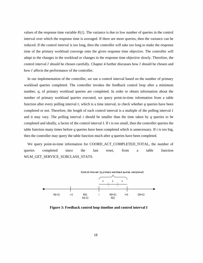
In our implementation of the controller, we use a control interval based on the number of primary

workload queries completed. The controller invokes the feedback control loop after a minimum

number, q, of primary workload queries are completed. In order to obtain information about the

number of primary workload queries executed, we query point-in-time information from a table

function after every polling interval 𝑡, which is a time interval, to check whether 𝑞 queries have been

completed or not. Therefore, the length of each control interval is a multiple of the polling interval 𝑡

and it may vary. The polling interval t should be smaller than the time taken by q queries to be

completed and ideally, a factor of the control interval I. If t is too small, then the controller queries the

table function many times before q queries have been completed which is unnecessary. If t is too big,

then the controller may query the table function much after q queries have been completed.

We query point-in-time information for COORD_ACT_COMPLETED_TOTAL, the number of

queries completed since the last reset, from a table function

WLM_GET_SERVICE_SUBCLASS_STATS.

Figure 3: Feedback control loop timeline and control interval I

19

Control Theory Logic

The feedback control loop in this framework is designed to use fundamentals from feedback control

theory [2] as its decision logic. Feedback control theory has been applied extensively in mechanical

systems [2]. Recently, it has started to become widely used a mathematical foundation for decision

making in control plans in computing [2, 11, 15].

In feedback-based control, depending on how the feedback information is used by the controller,

different levels of performance can be achieved. The simplest form of feedback-based control is

proportional control. If we use proportional control, the concurrency threshold variable 𝐶(𝑖) is

proportional to the error; 𝐶 𝑖 = 𝐾𝑃 ∗ 𝐸(𝑖) where 𝐾𝑃 is a tunable constant referred to as proportional

gain [2]. The effective result is to immediately react to the instantaneous error 𝐸(𝑖) to correct it.

Therefore, the disadvantage of proportional control is that it can react to short, transient disturbances

by immediately trying to correct it.

In contrast to proportional control, another form of feedback-based control is integral control. If we

use integral control, the change in the concurrency threshold variable 𝐶(𝑖) is governed by the error;

𝐶 𝑖 = 𝐶 𝑖 − 1 + 𝐾𝐼 ∗ 𝐸 𝑖 , where 𝐾𝐼 is a tunable constant [2]. The effective result is to accumulate

all the errors over time to determine the concurrency threshold.

𝐶 1 = 𝐶 0 + 𝐾𝐼 ∗ 𝐸 1

𝐶 2 = 𝐶 1 + 𝐾𝐼 ∗ 𝐸(2)

⋮

𝐶 𝑖 = 𝐶 0 + 𝐾𝐼 ∗ 𝐸 1 + 𝐾𝐼 ∗ 𝐸 2 + ⋯ + 𝐾𝐼 ∗ 𝐸(𝑖)

𝐶 𝑖 = 𝐶 0 + 𝐾𝐼 𝐸(𝑗)

𝑖

𝑗=1

Since integral control acts upon past errors, it tries to respond more to sustained change in response

time rather than short, transient disturbances in response time. Therefore, with databases workload

being prone to transient disturbances, we use integral control as our logic in the implementation of the

controller.

20

In our implementation of the controller, we choose to not completely shut out the secondary

workload queries from running. Therefore, we use the following to determine the concurrency

threshold so that we have at least one secondary workload query running in the system at all times.

𝐶 𝑖 = max 1, 𝐾𝐼 𝐸 𝑗

𝑖

𝑗=1

The integral constant 𝐾𝐼 defines the sensitivity of the controller’s output, i.e. the concurrency

threshold, to the error. From the integral control equation,

𝐶 𝑖 = 𝐶 𝑖 − 1 + 𝐾𝐼 ∗ 𝐸(𝑖)

𝐶 𝑖 − 𝐶 𝑖 − 1 = 𝐾𝐼 ∗ 𝐸(𝑖)

𝐾𝐼 =𝐶 𝑖 − 𝐶(𝑖 − 1)

𝐸(𝑖)

Therefore, 𝐾𝐼 is the amount by which the controller should manipulate the concurrency threshold

for a unit error in the response time of the primary workload.

If 𝐾𝐼 value is too high, then the feedback control loop makes large changes to the concurrency

threshold variable C(i) for a given error,. This can make the controller aggressive in responding to

errors, resulting in performance problems of overshoot and oscillation. If 𝐾𝐼 value is too low, then it

can result in making the feedback control loop too conservative in responding to errors in the

response time of the primary workload. This results in making the controller less sensitive to changes

in the system, such as changing workload. Hence, the value integral constant 𝐾𝐼 should be chosen

carefully. It should be noted that 𝐾𝐼 is specific to the workloads and the system being used. Therefore,

in our experiments presented in the next chapter, we choose 𝐾𝐼 experimentally, by trying different

values for 𝐾𝐼 to see how the feedback control loop reacts and tune the value accordingly. In Chapter

4, we further discuss how controller constant 𝐾𝐼 affect the performance of the controller.

3.2.1.3.3 Adaptive admission controller algorithm

Algorithm 1 shows how the adaptive admission controller works with the feedback control loop and

all of the variables defined. The algorithm consists of three steps: sample, calculate and manipulate.

These three functions constitute the feedback control loop described earlier in this section. The

21

sample step and calculate step make up the advisor sub-component and the manipulate step makes up

the effector sub-component.

Input: Polling interval 𝑡, Minimum query count 𝑞, Response time objective RS, Integral constant 𝐾𝐼

// Initialize number of completed primary workload queries and accumulated error

𝑛 = 0 and 𝐸 = 0;

while workloads run do

// Ensuring a control interval of a minimum of 𝑞 completed primary workload queries has lapsed

while 𝑛 < 𝑞 do

// Waiting idle for 𝑡 seconds before the number of completed primary workload queries is polled

wait 𝑡;

// Reading the number of completed primary workload queries since the last reset

𝑛 ⃪ Read COORD_ACT_COMPLETED_TOTAL from WLM_GET_SERVICE_SUBCLASS_STATS;

end

// 𝑺𝒂𝒎𝒑𝒍𝒆

// Measure response time average of primary workload from the statistics table

𝑅 ⃪ Read execution time average from SCSTATS_DB2STATISTICS;

// 𝑪𝒂𝒍𝒄𝒖𝒍𝒂𝒕𝒆

// Integrate error to implement integral control

𝐸 = 𝐸 + (𝑅𝑆 − 𝑅);

// Ensuring that at least one secondary workload query is allowed to run

𝐶 = max(1, 𝐾𝐼 ∗ 𝐸);

// 𝑴𝒂𝒏𝒊𝒑𝒖𝒍𝒂𝒕𝒆

// Half-up round C to integer

𝐶 = 𝑟𝑜𝑢𝑛𝑑 𝐶 ;

// Update concurrency threshold of secondary workload

Set CONCURRENTDBCOORDACTIVITIES to 𝐶;

Reset statistics by calling WLM_COLLECT_STATS();

end

Algorithm 1: Adaptive Admission Control

22

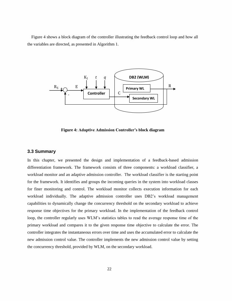
Figure 4 shows a block diagram of the controller illustrating the feedback control loop and how all

the variables are directed, as presented in Algorithm 1.

Primary WL

Secondary WL

Controller

DB2 (WLM)

R

C

E RS +

-

KI 𝑞 𝑡

Figure 4: Adaptive Admission Controller’s block diagram

3.3 Summary

In this chapter, we presented the design and implementation of a feedback-based admission

differentiation framework. The framework consists of three components: a workload classifier, a

workload monitor and an adaptive admission controller. The workload classifier is the starting point

for the framework. It identifies and groups the incoming queries in the system into workload classes

for finer monitoring and control. The workload monitor collects execution information for each

workload individually. The adaptive admission controller uses DB2’s workload management

capabilities to dynamically change the concurrency threshold on the secondary workload to achieve

response time objectives for the primary workload. In the implementation of the feedback control

loop, the controller regularly uses WLM’s statistics tables to read the average response time of the

primary workload and compares it to the given response time objective to calculate the error. The

controller integrates the instantaneous errors over time and uses the accumulated error to calculate the

new admission control value. The controller implements the new admission control value by setting

the concurrency threshold, provided by WLM, on the secondary workload.

23

Chapter 4

Experimental Evaluation

In this chapter, we evaluate the effectiveness of the admission controller in adaptively achieving

response time average objectives. Specifically, we address the following questions in this chapter:

1. Does admission control on the secondary workload affect the response time for the

primary workload?

2. Can the controller achieve response time objectives for a fixed workload?

3. Can the controller automatically adapt to changes in the response time objective of the

primary workload?

4. Can the controller dynamically adapt to changing workload conditions in the system?

5. How do input parameters such as controller constant KI and control interval I affect the

performance of the controller?

6. Will the controller work for workloads consisting of small queries, coming in at a high

arrival rate?

All the above questions are addressed experimentally. We designed a set of experiments to show

effectiveness of the controller in various scenarios. In Section 4.4, we present the results of an

experiment in which we test whether admission control is an effective choice for affecting the

response time of the primary workload. Then, we move on to experiments with the controller.

In the controller experiments, we evaluate the controller’s ability to achieve the response time

objective with minimal overshoot, minimal oscillation and short convergence time. Each controller

experiment is conducted by running the test workloads and the controller together for a period of 96

minutes on an instance of DB2. The controller is given the required response time objective RS,

controller constant KI, control interval I (shown as the minimum query count q) and polling interval t

as inputs.

In Section 4.5, we present the results of controller experiments in which we show the performance

of the controller on stable workloads with a fixed response time objective. In Section 4.6, we present

the results of controller experiments in which we test the controller in a scenario in which the

24

response time objective changes halfway through the experiment. In Section 4.7, we present the

results of controller experiments in which we test the controller in a scenario in which the workload

changes halfway through the experiment. In Section 4.8, we present the results of controller

experiments in which we show how controller constant KI and control interval I affect the

performance of the controller. In Section 4.9, we present the results of experiments in which we

examine the feasibility of using our controller’s admission control on workloads consisting of small

queries, coming in at a high arrival rate.

Before we address the questions related to the effectiveness of the controller, in Section 4.1, we

present the experimental system configuration used in the experiments. In Section 4.2, we present the

synthetic test workloads used in the experiments and in Section 4.3, we test the intensity of the

workloads to ensure that they will be useful in the experiments for testing the effectiveness of the

controller.

4.1 Experimental Test Bed

The database server machine used runs DB2 Version 9.5 on Linux kernel 2.6.5-7.283–smp (x86_64).

The system consists of four 2.0 GHz 64-bit Dual Core AMD Opteron (tm) processors. Therefore, the

system has 8 cores. However, the DB2 server’s fixed term license allows a maximum processor

utilization of 4 cores only. Hence, in our experiments, the DB2 database engine uses 4 CPU cores at

any given time. The threading degree is 1 thread per core. The system has 8 GB of RAM.

4.2 Database Workload Generator and Test Workloads

The workloads used to test the controller were generated using a database workload

generator called DWG. DWG is a Java program that generates read-only CPU bound workloads.

DWG begins by spawning a number of threads, each of which obtains a database connection to the

DB2 data server, and issues queries through the connections. DWG generates transactional

workloads with random query service time (TS) and query inter-arrival time (TA). DWG allows the

users to specify the distributions that the service times and the inter-arrival times should follow.

DWG is also capable of generating multiple concurrent workloads, each with a distinct, user-specified

query service and inter-arrival time distributions.

25

DWG defines and populates a set of tables against which its queries will be issued. A basic query

that DWG generates is to count the number of rows in the result of a join of many tables in the

database. In order to produce queries of various service times, variations of the basic query are

produced by performing a variable number of unions of the query with itself, thereby varying the

number of joins and the number of rows of the tables being queried.

DWG allows a user to choose from the following two types of distributions, according to which the

service times and the inter-arrival times are sampled:

1. Empirical distribution: DWG allows the user to specify an arbitrary, discrete cumulative

distribution function as a series of service time or inter-arrival time values and their

corresponding probabilities that the query service time or the query inter-arrival time is less

than or equal to the values. In our experiments, we use empirical distribution to simulate

workloads with deterministic, or fixed, service times or inter-arrival times by specifying a

probability of 1 for a fixed value to be sampled.

2. Exponential distribution: DWG can also generate exponentially distributed times with a user-

specified mean value. We use exponential distribution to generate workloads with random, or

variable, service times or inter-arrival times.

DWG also allows a user to specify a particular username for each workload so that DWG can

simulate the workload as if it is coming into the system from the particular username’s terminal.

DWG makes database connections to the DB2 data server for the queries from each workload with

the workload’s specified username. Therefore, we specify different usernames for the primary

workload and the secondary workload. We configure the workload classifier to identify primary

workload queries coming in from the same user and map them to one workload class and all the other

queries coming into the system from another user are considered secondary and mapped into another

workload class.

We design our test workloads’ service times and inter-arrival times in such a way that when both the

workloads run together, they overload the system, creating our problem scenario. We use the

following statistic to ensure high CPU utilization.

𝐶𝑃𝑈 𝑢𝑡𝑖𝑙𝑖𝑧𝑎𝑡𝑖𝑜𝑛 =𝑚𝑒𝑎𝑛 𝑠𝑒𝑟𝑣𝑖𝑐𝑒 𝑡𝑖𝑚𝑒

𝑚𝑒𝑎𝑛 𝑖𝑛𝑡𝑒𝑟-𝑎𝑟𝑟𝑖𝑣𝑎𝑙 𝑡𝑖𝑚𝑒

26

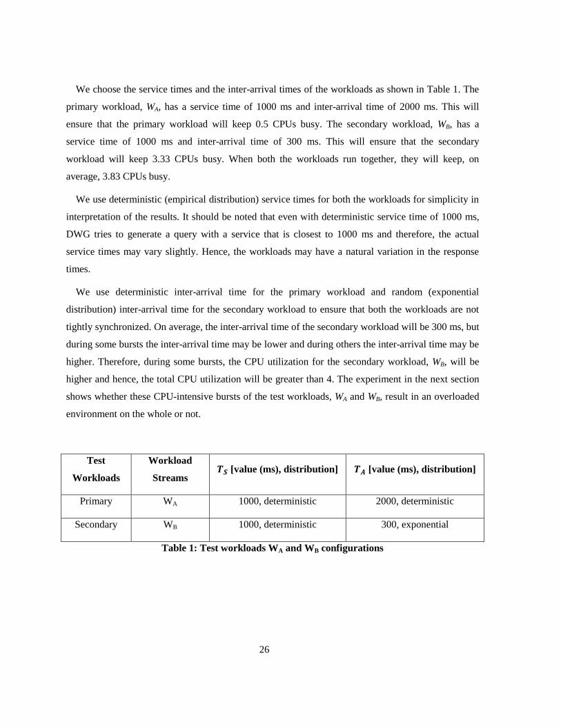
We choose the service times and the inter-arrival times of the workloads as shown in Table 1. The

primary workload, WA, has a service time of 1000 ms and inter-arrival time of 2000 ms. This will

ensure that the primary workload will keep 0.5 CPUs busy. The secondary workload, WB, has a

service time of 1000 ms and inter-arrival time of 300 ms. This will ensure that the secondary

workload will keep 3.33 CPUs busy. When both the workloads run together, they will keep, on

average, 3.83 CPUs busy.

We use deterministic (empirical distribution) service times for both the workloads for simplicity in

interpretation of the results. It should be noted that even with deterministic service time of 1000 ms,

DWG tries to generate a query with a service that is closest to 1000 ms and therefore, the actual

service times may vary slightly. Hence, the workloads may have a natural variation in the response

times.

We use deterministic inter-arrival time for the primary workload and random (exponential

distribution) inter-arrival time for the secondary workload to ensure that both the workloads are not

tightly synchronized. On average, the inter-arrival time of the secondary workload will be 300 ms, but

during some bursts the inter-arrival time may be lower and during others the inter-arrival time may be

higher. Therefore, during some bursts, the CPU utilization for the secondary workload, WB, will be

higher and hence, the total CPU utilization will be greater than 4. The experiment in the next section

shows whether these CPU-intensive bursts of the test workloads, WA and WB, result in an overloaded

environment on the whole or not.

Test

Workloads

Workload

Streams 𝑻𝑺 [value (ms), distribution] 𝑻𝑨 [value (ms), distribution]

Primary WA 1000, deterministic 2000, deterministic

Secondary WB 1000, deterministic 300, exponential

Table 1: Test workloads WA and WB configurations

27

4.3 Experiment 1: Effect of WB on WA

As explained in Chapter 1, our controller is targeted at achieving performance objectives for the

primary workload WA in a problem scenario where the secondary workload WB overloads the system

and competes with WA for CPU resources. Therefore, in order to examine the effect of WB on WA, we

conducted this characterization experiment. In this experiment, we compare the performance of each

workload when run in isolation with the performance of the workloads when run together.

Essentially, we compare the performance of WA when there is no CPU contention with the

performance of WA in an overloaded system in which there is there is competition for CPU resources.

In this experiment, we performed three runs with a runtime of 96 minutes each. First, WA is run in

isolation and the response time average is measured every 30 seconds (for calculation of variance in

the response time average measurements) over the run. Second, WB is run in isolation and the

response time average is measured every 30 seconds over the run. Third, WA and WB are run together

and their response time averages are measured every 30 seconds over the run. The first two runs serve

as the baseline measure for the third run. The third run is for examining whether the workloads

together overload the system, which is confirmed by a significant increase in response time averages

of both the workloads.

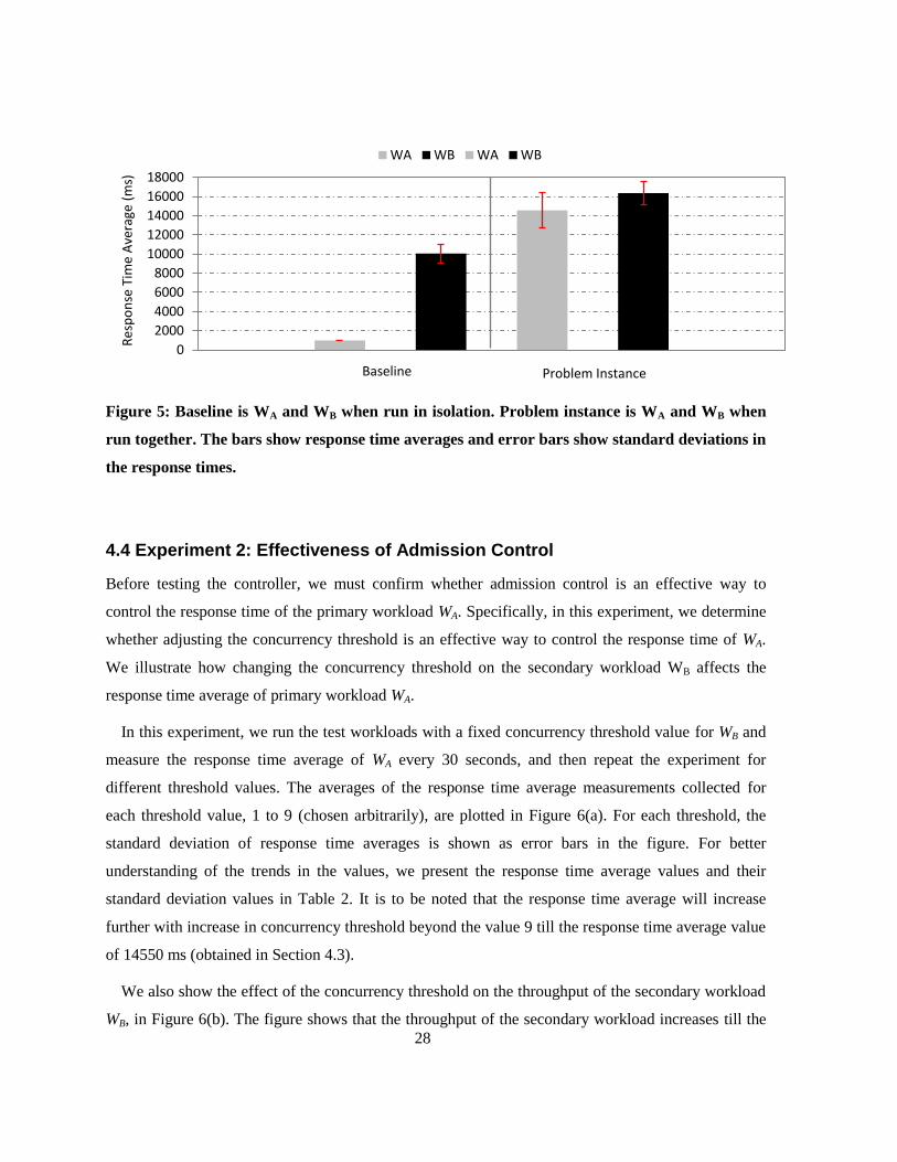
Figure 5 shows the averages of the response time average measurements of all the runs. The

response time average of WA when run in isolation is nearly 1000 ms with a very low standard

deviation of 0.7. This is because of using a deterministic service time of 1000 ms for WA, which

confirms that the response time of WA does not have a significant natural variation. When WA and WB

are run together, we see a significant deterioration in the performances of WA and WB. Most

importantly, the response time average of the primary workload WA increased to 14550 ms, which is

14 times that of WA when run in isolation. This result confirms that the secondary workload WB

competes for CPU resources with the primary workload WA, thereby deteriorating the response time

average of the primary workload WA. Therefore, the workloads WA and WB when run together create a

good test instance of our problem scenario, on which our admission controller mechanism can be

tested.

28

Figure 5: Baseline is WA and WB when run in isolation. Problem instance is WA and WB when

run together. The bars show response time averages and error bars show standard deviations in

the response times.

4.4 Experiment 2: Effectiveness of Admission Control

Before testing the controller, we must confirm whether admission control is an effective way to

control the response time of the primary workload WA. Specifically, in this experiment, we determine

whether adjusting the concurrency threshold is an effective way to control the response time of WA.

We illustrate how changing the concurrency threshold on the secondary workload WB affects the

response time average of primary workload WA.

In this experiment, we run the test workloads with a fixed concurrency threshold value for WB and

measure the response time average of WA every 30 seconds, and then repeat the experiment for

different threshold values. The averages of the response time average measurements collected for

each threshold value, 1 to 9 (chosen arbitrarily), are plotted in Figure 6(a). For each threshold, the

standard deviation of response time averages is shown as error bars in the figure. For better

understanding of the trends in the values, we present the response time average values and their

standard deviation values in Table 2. It is to be noted that the response time average will increase

further with increase in concurrency threshold beyond the value 9 till the response time average value

of 14550 ms (obtained in Section 4.3).

We also show the effect of the concurrency threshold on the throughput of the secondary workload

WB, in Figure 6(b). The figure shows that the throughput of the secondary workload increases till the

0

2000

4000

6000

8000

10000

12000

14000

16000

18000

Res

po

nse

Tim

e A

vera

ge (

ms)

WA WB WA WB

Problem InstanceBaseline

29

value 3.2 and then levels off at the same value. This is because the average CPU utilization of the

secondary workload, as explained in Section 4.2, is 3.33. With the concurrency threshold being an

upper bound on the number of concurrent queries that can execute at a time, the secondary workload

was able to execute only as many queries as the threshold value till it reached its maximum

concurrency at threshold 4. At concurrency threshold 4 and higher, the secondary workload was able

to run close to its maximum concurrency of 3.33.

Figure 6: Sensitivity to concurrency threshold on WB. (a) shows response time average of WA

for each concurrency threshold on WB. (b) shows throughput of WB for each concurrency

threshold on WB. Error bars indicate standard deviation in the measurements at each

concurrency threshold.

0.00

500.00

1000.00

1500.00

2000.00

2500.00

3000.00

1 2 3 4 5 6 7 8 9

Res

po

nse

Tim

e A

vera

ge_W

A (

ms)

Threshold(a) Response time average of WA

00.5

11.5

22.5

33.5

4

1 2 3 4 5 6 7 8 9

Thro

ugh

pu

t_W

B

(qu

erie

s/se

con

d)

Threshold(b) Throughput of WB

30

Concurrency threshold (C) Response time average Standard deviation (𝝈𝑪)

1 1058 1.38

2 1082 6.84

3 1105 7.46

4 1682 106.14

5 1824 135.70

6 1970 149.55

7 2231 172.56

8 2462 189.78

9 2641 210.31

Table 2: Response time average and standard deviation of WA for each concurrency threshold

C from Figure 6(a)

In Figure 6(a), there are two slopes in the trend of the response time averages of WA. The figure

shows that an increase in concurrency threshold value from 1 to 3 resulted in a barely noticeable

increase in the response time average of WA. The slope of the (best fit) line is 23. For increase in

concurrency threshold value from 4 to 9, there was a significant increase in the response time average

of WA. The slope of the (best fit) line is 225, which is nearly 10 times that of the slope for thresholds 1

to 3. The following is the explanation for the two distinct trends:

1. The trend of thresholds 1 to 3 exemplifies a no-CPU-contention environment; the total

concurrency of both the workloads together in the system is less than 4, which is number of

CPU cores in the system. Therefore, there is one-to-one mapping between queries and each

CPU core. Each query will have a dedicated CPU core. Hence, each query will have

negligible wait time TW. Therefore, the changing concurrency threshold on WB isn`t reflected

much on the response time average of WA.

2. The trend of thresholds 4 to 9 exemplifies a CPU-contention environment; the total number

of concurrent queries of both the workloads together in the system can be more than 4

31

sometimes. During the bursts in which the inter-arrival time of WB is smaller than 300 ms,

the queries that exceed the concurrency threshold applied are queued. Hence, as and when the

number of concurrent WB queries drops below the threshold, there are always queued queries

ready to run and increase the number of concurrent WB queries to the threshold value.

Therefore, effectively, there can be threshold number of WB queries running concurrently in

the system. Hence, there can be many-to-one mapping between queries and each CPU core.

The queries are multiplexed between the CPU cores through context-switching and

scheduling. Therefore, with increase in concurrency, there will be significant increase in

context switches for each query and hence, there will be significant increase in CPU wait

time TW for each query. Therefore, each unit value change in concurrency threshold on WB

results in a significant change in the response time average of WA.

Apart from these two significant trends, there is a steep slope from threshold value 3 to 4. This is

due to a spike in the response time average of WA at threshold 4. At threshold 4, WB performs at its

maximum concurrency and therefore, tries to keep more than 3 CPU cores busy, on average. Since

WA requires at least one CPU core, it faces significant competition from WB for that one CPU core

because there are only 4 CPU cores in the system. Hence, the response time average of WA increases

steeply at threshold 4.

Similar to the significant trends in response time averages of WA, there are two trends for the

variance in the response time measurements of the primary workload WA (in Table 2). The trend for

standard deviation 𝜎𝐶 for each concurrency threshold C is as follows:

1. Thresholds 1 to 3: As it is expected with a stable primary workload with no significant

natural variation in a no-CPU-contention environment, the figure shows small standard

deviations for these thresholds. For example, 𝜎1 = 1.38, 𝜎2 = 6.84 and 𝜎3 = 7.46.

2. Thresholds 4 to 9: The response time average measurements aren’t stable enough because the

measurements are dominated by the variance brought in due to resource contention, which

brings in context switching and scheduling overhead. For example, 𝜎4 = 106.14 and 𝜎5 =

135.70 which are nearly 10 times that of threshold 1.

32

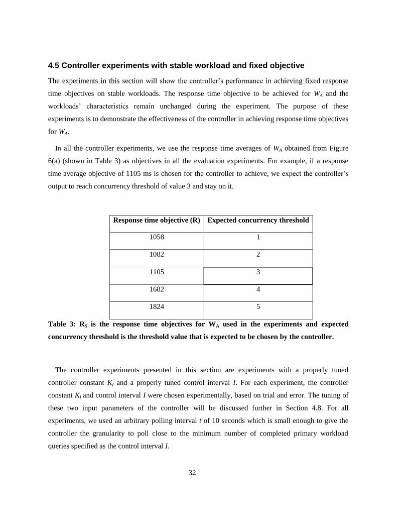
4.5 Controller experiments with stable workload and fixed objective

The experiments in this section will show the controller’s performance in achieving fixed response

time objectives on stable workloads. The response time objective to be achieved for WA and the

workloads’ characteristics remain unchanged during the experiment. The purpose of these

experiments is to demonstrate the effectiveness of the controller in achieving response time objectives

for WA.

In all the controller experiments, we use the response time averages of WA obtained from Figure

6(a) (shown in Table 3) as objectives in all the evaluation experiments. For example, if a response

time average objective of 1105 ms is chosen for the controller to achieve, we expect the controller’s

output to reach concurrency threshold of value 3 and stay on it.

Response time objective (R) Expected concurrency threshold

1058 1

1082 2

1105 3

1682 4

1824 5

Table 3: RS is the response time objectives for WA used in the experiments and expected

concurrency threshold is the threshold value that is expected to be chosen by the controller.

The controller experiments presented in this section are experiments with a properly tuned

controller constant KI and a properly tuned control interval I. For each experiment, the controller

constant KI and control interval I were chosen experimentally, based on trial and error. The tuning of

these two input parameters of the controller will be discussed further in Section 4.8. For all

experiments, we used an arbitrary polling interval t of 10 seconds which is small enough to give the

controller the granularity to poll close to the minimum number of completed primary workload

queries specified as the control interval I.

33

For each controller experiment, four graphs are presented to show the dynamics of the workloads

as a function of time:

The first graph shows the response time average R(i) of primary workload measured after

each control interval. We expect the primary workload to achieve its response time objective

RS with minimal overshoot and oscillation and stabilize on the objective.

The second graph shows the controller output C(i), the new, calculated concurrency threshold

the controller applies on secondary workload after each control interval. We expect it to reach

the expected concurrency threshold corresponding to the objective shown in Table 3 with

minimal overshoot and oscillation and stabilize on the threshold.

The third graph shows the throughput of secondary workload during each control interval.

We expect it to increase when the concurrency threshold applied on the secondary workload

increases and decrease when the concurrency threshold applied on the secondary workload

decreases.

The fourth graph shows the response time average of the secondary workload measured after

each control interval. We expect it to decrease with an increase in the concurrency threshold

applied on the secondary workload and increase with a decrease in the concurrency threshold

applied on the secondary workload.

4.5.1 Controller Experiment 1: RS = 1082, KI = 0.01, I = 20

In this experiment, we use a response time average objective RS of 1082 ms. The purpose of this

experiment is to test whether the controller is able to achieve an objective from the no-CPU-

contention environment. We expect the controller to stabilize on concurrency threshold 2 with

minimal overshoot and oscillation.

We perform this experiment with a controller constant KI of value 0.01 and a control interval I of a

minimum of 20 primary workload queries. Figure 7 shows the results of this experiment. The

controller output graph (in Figure 7(b)) shows that the controller output C(i) reaches the expected

concurrency threshold 2 in 280 seconds (7 control steps, each after an interval of 40 seconds) and as

a result, the response time average R(i) (in Figure 7(a)) also reaches the desired objective 1082

ms. The figure shows that the controller understands that if the response time average R(i) of the

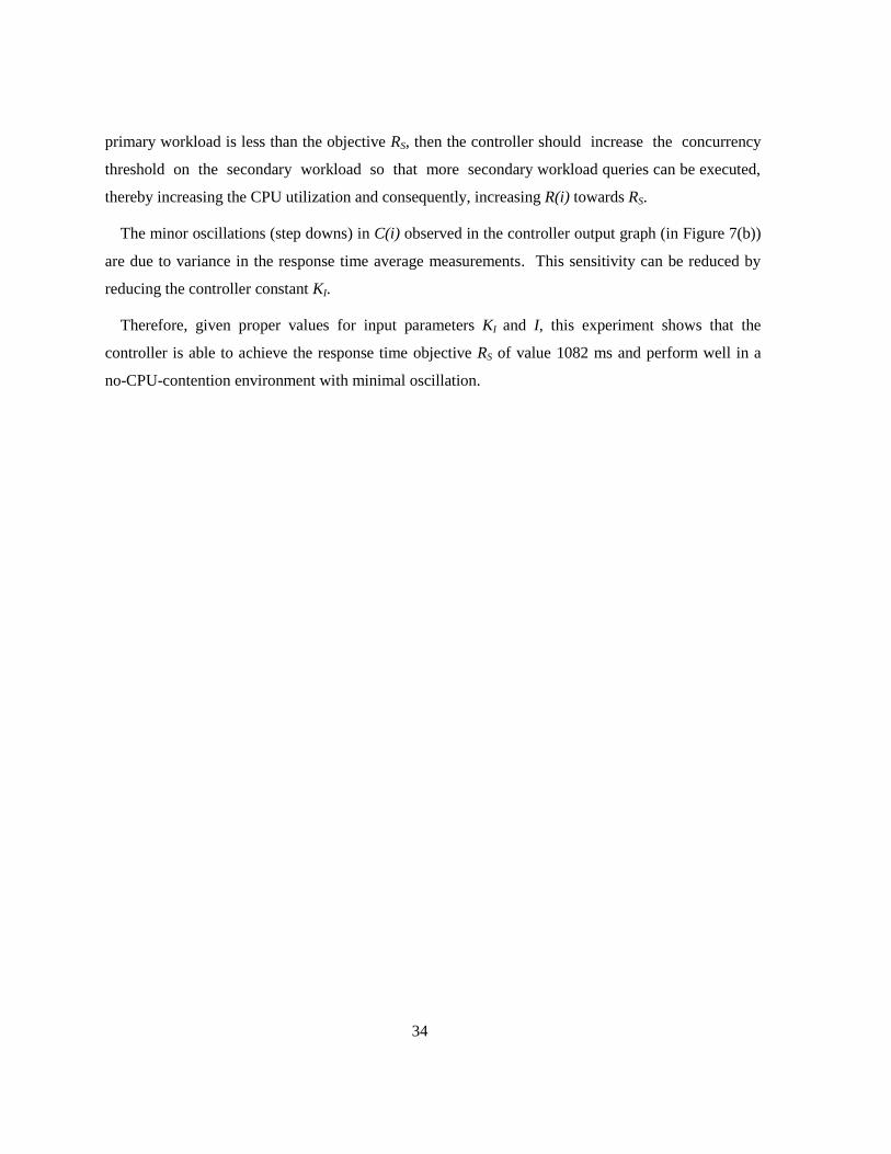
34

primary workload is less than the objective RS, then the controller should increase the concurrency

threshold on the secondary workload so that more secondary workload queries can be executed,

thereby increasing the CPU utilization and consequently, increasing R(i) towards RS.

The minor oscillations (step downs) in C(i) observed in the controller output graph (in Figure 7(b))

are due to variance in the response time average measurements. This sensitivity can be reduced by

reducing the controller constant KI.

Therefore, given proper values for input parameters KI and I, this experiment shows that the

controller is able to achieve the response time objective RS of value 1082 ms and perform well in a

no-CPU-contention environment with minimal oscillation.

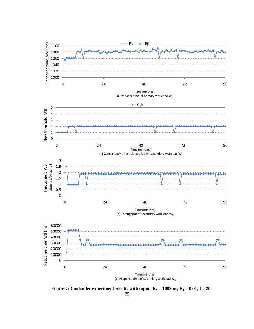
35

Figure 7: Controller experiment results with inputs RS = 1082ms, KI = 0.01, I = 20

1000

1020

1040

1060

1080

1100

0 24 48 72 96Res

po

nse

tim

e_W

A (

ms)

Time (minutes)(a) Response time of primary workload WA

Rs R(i)

0

1

2

3

4

5

0 24 48 72 96

New

th

resh

old

_WB

Time (minutes)(b) Concurrency threshold applied on secondary workload WB

C(i)

0

0.5

1

1.5

2

2.5

3

0 24 48 72 96

Thro

ugh

pu

t_W

B

(qu

erie

s/se

con

d)

Time (minutes)(c) Throughput of secondary workload WB

0

10000

20000

30000

40000

50000

60000

0 24 48 72 96

Res

po

nse

tim

e_W

B (

ms)

Time (minutes)(d) Response time of secondary workload WB

36

4.5.2 Controller Experiment 2: RS = 1682ms, KI = 0.001, I = 40

In this experiment, we use a response time average objective RS of 1682 ms. The purpose of this

experiment is to test whether the controller is able to achieve a response time average objective from

the CPU-contention environment. We expect the controller to stabilize on concurrency threshold 4

with minimal overshoot and oscillation.

We perform this experiment with a controller constant KI of value 0.001 and a control interval I of a

minimum of 40 completed primary workload queries. Figure 8 shows the results of this experiment.

The controller output graph (Figure 8(b)) shows that the controller output C(i) smoothly climbs to the

expected threshold 4 in 480 seconds (6 control steps, each after an interval of 80 seconds).

Correspondingly, the response time average R(i) (in Figure 8(a)) also steadily climbs to the desired

objective 1682 ms.

Compared to Controller Experiment 1, a smaller controller constant KI of value 0.001 and a longer

control interval I of a minimum of 40 completed primary workload queries worked well in this

experiment because the response time objective 1682 ms belongs to the CPU-contention environment.

For the CPU-contention environment, as explained in Experiment 2, the (slope of) change in response

time average of primary workload for a unit change in concurrency threshold on secondary workload

is higher. This results in larger changes in response time when the controller changes the concurrency

threshold. Therefore, a smaller controller constant KI compensates for the larger changes in response

time that the controller makes. In addition, for the CPU-contention environment, the variance in the

response time averages of the primary workload is higher. Therefore, a longer control interval I

dampens the variance and allows the controller to stay on the response time objective 1682 ms with

minimal oscillation.

Therefore, given appropriate values for input parameters KI and I, this experiment shows that the

controller is able to achieve the response time objective RS of value 1682 ms and perform well in a

CPU-contention environment with minimal oscillation.

37

Figure 8: Controller experiment results with inputs: RS = 1682ms, KI = 0.001, I = 40

1000

1400

1800

2200

2600

3000

0 24 48 72 96

Res

po

nse

tim

e_W

A (

ms)

Time (minutes)(a) Response time of primary workload WA

Rs R(i)

0

1

2

3

4

5

0 24 48 72 96New

th

resh

old

_WB

Time (minutes)(b) Concurrency threshold applied on secondary workload WB

C(i)

00.5

11.5

22.5

33.5

0 24 48 72 96

Thro

ugh

pu

t (q

uer

ies/

seco

nd

)

Time (minutes)(c) Throughput of secondary workload WB

0

10000

20000

30000

40000

50000

60000

0 24 48 72 96

Res

po

nse

tim

e_W

B (

ms)

Time (minutes)(d) Response time of secondary workload WB

38

4.5.3 Conclusion

The experiments in this section show that our adaptive admission controller can achieve

response time objectives for the primary workload by applying admission control on the

secondary workload, provided that appropriate values are set for controller constant KI and

control interval I. The controller is able to perform well without any performance problems in

environments without CPU contention in Experiment 1 and with CPU contention in Experiment 2.

4.6 Controller Experiments with Stable Workload and Changing Objective

In this section, we test our controller in a scenario in which the response time objective changes. In

these experiments, the response time objective RS of primary workload is changed half-way through

the experiment. The purpose of these experiments is to show how the controller automatically

adapts to changes in the response time objective.

In these experiments, when the response time objective RS changes, it results in significant error

in the comparison of the measured response time average R(i) of the primary workload and the

objective RS. Therefore, the controller calculates and applies a new threshold on the secondary

workload and then the response time average of the primary workload changes accordingly.

Essentially, the change is initiated by the controller output that consequently directs the running

response time average towards the objective.

For experiments in this section, after experimental tuning, we use a controller constant KI of

value of 0.01 for objectives from the no-CPU-contention environment. We use a KI of value 0.001

for objectives from the CPU-contention environment. I f we have objectives from both the

environments, we use a KI value of 0.01/6 which is midway between values 0.01 and 0.001.

Similarly, we use a control interval I of a minimum of 20 primary workload queries for

objectives from a no-CPU-contention environment and a minimum of 40 primary workload

queries when there is an objective from a CPU-contention environment involved.

4.6.1 Controller Experiment 3: RS = 1058ms -> 1082ms

In this experiment, the controller is tested for a response time objective change of a small

magnitude from 1058 ms to 1082 ms. The challenge for the controller in this experiment is that we

39

change from a response time objective corresponding to a lower concurrency threshold to a

response time objective corresponding to a higher concurrency threshold. Therefore, when the

objective changes, we expect the controller output to increase from threshold 1, which is the

expected concurrency threshold for objective 1058 ms, to threshold 2, which is the expected

concurrency threshold for objective 1082 ms, with minimal overshoot and oscillation.

We use a controller constant KI of value 0.01 and a control interval I of a minimum of 20

primary workload queries because both the objectives 1058 ms and 1082 ms correspond to

thresholds from the no-CPU-contention environment.

Figure 9 shows the results of this experiment. The controller output graph (in Figure 9(b))

shows that after the objective changes, the controller output C(i) successfully increases from

threshold 1 to threshold 2. Therefore, the controller understands that if the response time objective of

WA increases, then it has to increase the concurrency threshold on WB so that more WB queries can

execute, thereby increasing WB’s CPU utilization and consequently, increasing the response time

average R(i) of WA (in Figure 9(a)) towards the objective RS.

The figure shows that the controller successfully achieved both the objectives with minimal

overshoot and oscillation. However, the controller output C(i) took a long time of 480 seconds

(12 control steps, each after an interval of 40 seconds) to converge onto the expected threshold 2.

This is because of a transient spike in the response time average of WA at the first control step.

The spike is due to test workload’s start up disturbance. The controller measured a high response

time average and as a result, the accumulated error of the controller significantly reduced to

negative error and continued to be there because it was still achieving the objective of 1058 ms by

applying the minimum concurrency threshold value of 1 on WB. Therefore, when the objective

changed, it took a long time for the accumulated error to increase from the negative error and

accumulate enough positive error for the controller output C(i) to increase up to threshold 2. This

shows that such transient disturbances in the system can lengthen the convergence time for the

controller. The convergence time can be decreased by increasing the controller constant KI for the

controller to take larger control steps or decrease the control interval I for the controller to take more

control steps per unit time.

This experiment shows that the controller is able to automatically handle a response time

objective increase by a small magnitude without any performance problems of overshoot and

oscillation.

40

Figure 9: Controller experiment results with inputs: RS = 1058ms->1082ms, KI = 0.01, I = 20

1000

1050

1100

1150

1200

0 24 48 72 96Res

po

nse

tim

e_W

A (

ms)

Time (minutes)(a) Response time of primary workload WA

Rs R(i)

0

1

2

3

4

5

0 24 48 72 96

New

th

resh

old

_WA

(m

s)

Time (minutes)(b) Concurrency threshold applied on secondary workload WB

C(i)

0

2

4

6

8

0 24 48 72 96

Thro

ugh

pu

t_W

B

(qu

erie

s/se

con

d)

Time (minutes)(c) Throughput of secondary workload WB

0100002000030000400005000060000

0 24 48 72 96

Res

po

nse

tim

e_W

B (

ms)

Time (minutes)(d) Response time of secondary workload WB

41

4.6.2 Controller Experiment 4: RS = 1105ms -> 1058ms

In this experiment, we tested the controller for a response time objective decrease of a small

magnitude from 1105 ms to 1058 ms. The challenge for the controller in this experiment is that we

change from a response time objective corresponding to a higher concurrency threshold to a response

time objective corresponding to a lower concurrency threshold. Therefore, when the objective

changes, we expect the controller output to decrease from concurrency threshold 3, which is the

expected concurrency threshold for objective 1105 ms, to threshold 1, which is the expected

concurrency threshold for objective 1058 ms.

Similar to previous experiment, we use a controller constant KI of 0.01 and a control interval I of a

minimum of 20 primary workload queries in this experiment.

Figure 10 shows the results of this experiment. The controller output graph (in Figure 10(b)) shows

that after the objective changes, the controller output C(i) successfully decreases from threshold 3 to

threshold 1. This shows that the controller understands that if the response time objective of WA

decreases, then it has to decrease the concurrency threshold on WB so that fewer WB queries execute in

the system, thereby decreasing WB’s CPU utilization and consequently, decreasing the response time

average of WA towards the objective RS.

The figure shows that the controller successfully achieved both of the response time objectives

without overshoot and oscillation. The controller output graph in the figure shows that before the

objective changed, the controller output C(i) converged onto the expected threshold 3 in 280 seconds

(7 control steps, each after an interval of 40 seconds) and after the objective changed, the controller

output converged onto the expected threshold 1 in 120 seconds (3 control steps). Correspondingly, the

response time average R(i) of WA (in Figure 10(a)) also steadily converged onto the respective

objective RS.

This experiment shows that the controller is able to dynamically handle a response time

objective decrease by a small magnitude without any performance problems.

42

Figure 10: Controller experiment results with inputs: RS = 1105ms->1058ms, KI = 0.01, I = 20

1000

1050

1100

1150

1200

1250

1300

0 24 48 72 96

Res

po

nse

tim

e_W

A (

ms)

Time (minutes)(a) Response time of primary workload WA

R(i) R

0

1

2

3

4

5

0 24 48 72 96

New

th

resh

old

_WB

)

Time (minutes)(b) Concurrency threshold applied on secondary workload WB

C(i)

0

1

2

3

4

0 24 48 72 96

Thro

ugh

pu

t (q

uer

ies/

seco

nd

)

Time (minutes)(c) Throughput of secondary workload WB

0

10000

20000

30000

40000

50000

60000

0 24 48 72 96

Res

po

nse

tim

e_W

B (

ms)

Time (minutes)(d) Response time of secondary workload WB

43

4.6.3 Controller Experiment 5: RS = 1824ms -> 1058ms

In this experiment, we tested the controller for a response time objective change of a large magnitude

from 1824 ms to 1058 ms. When the objective changes, we expect the controller output to decrease

from concurrency threshold 5, which is the expected concurrency threshold for objective 1824 ms, to

concurrency threshold 1, which is the expected concurrency threshold for objective 1058 ms.

We know that a lower controller constant KI of value 0.001 works for the objective 1824 ms

because it belongs to the CPU-contention environment. We know that a higher controller constant KI

of value 0.01 works for the objective 1058 ms because it belongs to the resource-sufficient

environment. In this experiment, we have both the objectives and therefore, we use a KI of value in

between 0.01 and 0.001 that works reasonably well for both the objectives. We found a KI of a value

0.01/6 to work the best. We use a control interval I of a minimum of 40 primary workload queries in

this experiment.

Figure 11 shows the results of this experiment. The controller output graph (in Figure 11(b)) shows

that when the objective decreases by a large magnitude, the controller output C(i) drops and continues

to drop until the expected threshold 1. This shows that the controller continues to make changes to the

concurrency threshold as long as there is any error in the comparison of the response time average

R(i) and the response time objective RS. The controller constantly strives to achieve zero error and

consequently, it strives to achieve the objective RS.

The results in the figure shows there were no performance problems of overshoot and oscillation

due to change in response time objective. The controller successfully achieved both the response time

objectives. The controller output graph in the figure shows that before the objective changed, the

controller output C(i) converged onto the expected threshold 5 in 320 seconds (4 control steps, each

after an interval of 80 seconds). After the objective changed, for objective 1058 ms from the no-CPU-

contention environment, as expected with a smaller control constant KI and a longer control interval I,

the controller output C(i) took a longer time of 1440 seconds (18 control steps) to converge onto the

expected threshold 1 in comparison to the previous experiments with objective 1058 ms.

Correspondingly, the response time average R(i) of WA (in Figure 11(a)) also steadily converged onto

the respective objective RS.

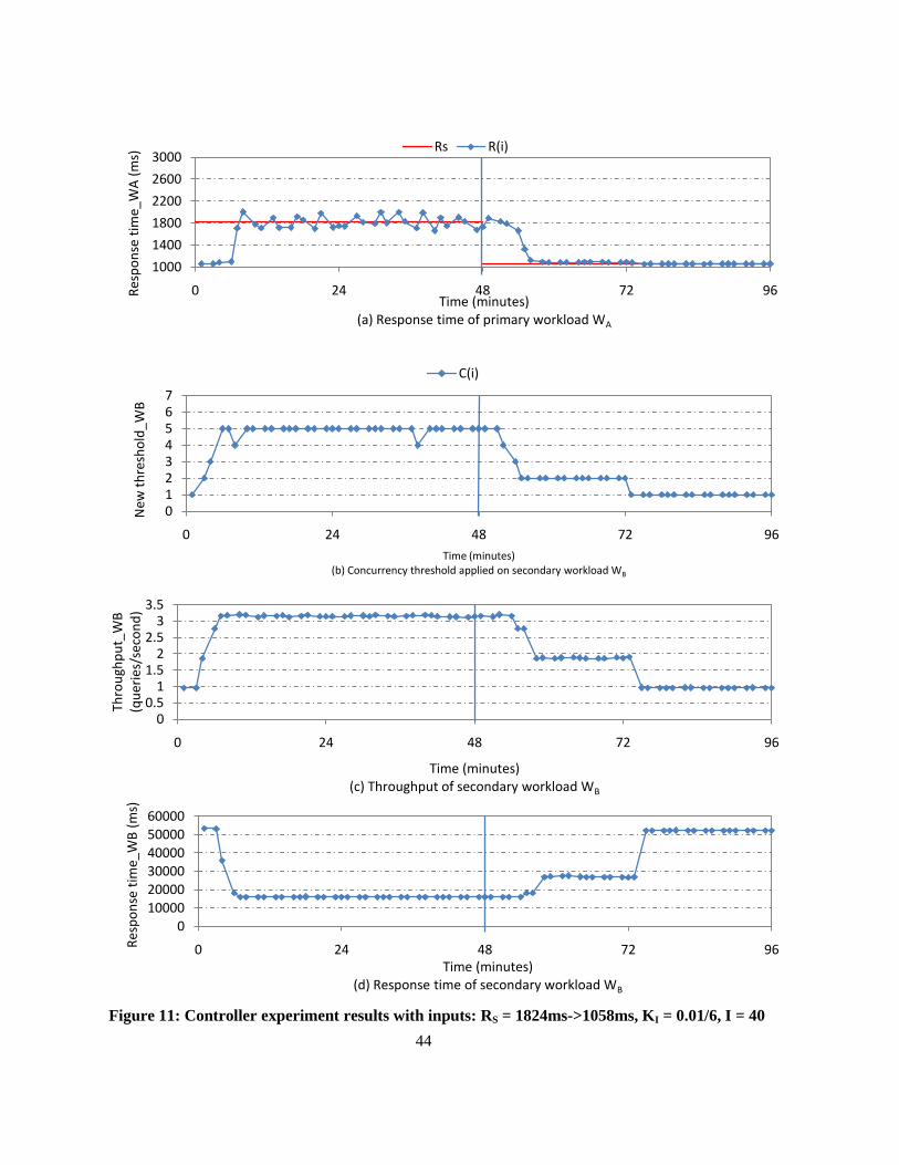
44

Figure 11: Controller experiment results with inputs: RS = 1824ms->1058ms, KI = 0.01/6, I = 40

1000

1400

1800

2200

2600

3000

0 24 48 72 96Res

po

nse

tim

e_W

A (

ms)

Time (minutes)(a) Response time of primary workload WA

Rs R(i)

01234567

0 24 48 72 96

New

th

resh

old

_WB

Time (minutes)(b) Concurrency threshold applied on secondary workload WB

C(i)

00.5

11.5

22.5

33.5

0 24 48 72 96

Thro

ugh

pu

t_W

B

(qu

erie

s/se

con

d)

Time (minutes)(c) Throughput of secondary workload WB

0

10000

20000

3000040000

50000

60000

0 24 48 72 96Res

po

nse

tim

e_W

B (

ms)

Time (minutes)(d) Response time of secondary workload WB

45

4.6.4 Conclusion

All the experiments in this section show that the controller can dynamically handle a change in the

response time objective RS. When the objective changes, the controller measures the change

through the error calculated when comparing the response time average R(i) of the primary

workload with the response time objective RS. As a result, the controller makes appropriate

changes to the concurrency threshold C(i) on the secondary workload and thereby, regulating the

number of queries executing in the system so that the response time average R(i) is directed

towards the objective RS. There were no performance problems of overshoot and oscillation due

to a change in the response time objective during the length of the experiments.

4.7 Controller Experiments with Changing Workloads and Fixed Objective

In this section, we test the adaptability of controller to a change in workload on the system. In these

experiments, the workload is changed after every 1/3rd

of the experiment. Specifically, we test the

controller`s ability to adapt to a change in CPU utilization due to change in the total number of

concurrent queries running in the system.

We design a workload stream WC to add to the primary workload in these experiments. Note that

we add the stream to the primary workload and not to the secondary workload because adding a

stream to the secondary workload will not be useful towards our intention to change the total number

of concurrent queries running in the system. Any added concurrency to the secondary workload will

end up queuing due to concurrency threshold, resulting in no increase in the CPU utilization.

For workload stream WC, we choose a deterministic service time of 1000 ms and a deterministic

inter-arrival time of 4000 ms. When this workload stream is added after every 1/3rd

of the experiment,

it should add to the CPU utilization on the system by keeping another 0.25 CPUs busy.

Workload Stream 𝑻𝑺 [value (ms), distribution] 𝑻𝑨 [value (ms), distribution]

WC 1000, deterministic 4000, deterministic

Table 4: Test workload WC configuration

46

In these experiments, a change in workload results in change in the response time average R(i) of

the primary workload and consequently, results in significant error in the comparison of R(i) and the

response time objective RS. Due to increased error, the controller output C(i) changes. Contrary to the

response time objective change experiments, in these experiments, the change is initiated by the

response time average R(i) of the primary workload that directs the controller output C(i) on the

secondary workloads.

In these experiments, since we work with changing workload, we also get to evaluate the controller

for a response time objective RS that does not correspond exactly to any concurrency threshold. We

conduct all the experiments with an arbitrarily chosen response time objective of 1105 ms.

4.7.1 Controller Experiment 6: Workload increase

In this experiment, the workload on the system is increased by a large magnitude after every 1/3rd

of

the experimental runtime. We add workload stream WC to the primary workload WA at the beginning

of the experiment and after every 32 minutes into the experiment. Therefore, the workloads in the

three phases of the experiment are shown in Table 5.

Phase Primary workload Secondary workload

1 WA+WC WB

2 WA+WC+WC WB

3 WA+WC+WC+WC WB

Table 5: Workloads in each phase of Experiment 6

The purpose of this experiment is to study how the controller adapts to workload increases. The

challenge in this experiment is that we change from a workload with the response time objective 1105

ms corresponding to a higher concurrency threshold value to a workload with the response time

objective 1105 ms corresponding to a lower concurrency threshold. Therefore, when the workload

47

increases, we expect the controller output to decrease and converge onto the right concurrency

threshold corresponding to the objective or toggle between two thresholds, between which the

objective exists.

We perform this experiment with a controller constant KI of value 0.01/6 and a control interval I of

a minimum of 20 primary workload queries. Figure 12 shows the results of this experiment. In Figure

12(a), in the first phase, the response time objective 1105 ms corresponds to concurrency

threshold 2 and therefore, the controller output C(i) (in Figure 12(b)) settles on threshold 1. The

controller output C(i) converges onto the expected threshold 2 in 460 seconds. In the second phase,

the objective 1105 ms shifts to corresponding to a concurrency threshold value lying in between

thresholds 1 and 2 and therefore, C(i) oscillates between the thresholds 1 and 2. In the third phase, the

objective 1105 ms shifts to corresponding to concurrency threshold 1 and therefore, the controller

output settles on threshold 1. The effect of the shift due to workload changes can be seen in the

throughput and the response time graphs of the secondary workload WB too.

This experiment shows that the controller is able to dynamically adapt to increase in workload, i.e.

increase in CPU utilization, without any performance problems due to a change in the workload.

48

Figure 12: Controller experiment results with inputs: RS = 1105ms, KI = 0.01/6, I = 20

1000

1100

1200

1300

1400

1500

1600

0 24 48 72 96

Res

po

nse

tim

e (m

s)

Time (minutes)(a) Response time of primary workload WA

Rs R(i)

0

1

2

3

4

5

0 24 48 72 96

New

th

resh

old

_WB

Time (minutes)(b) Concurrency threshold applied on secondary workload WB

C(i)

0

0.5

1

1.5

2

2.5

0 24 48 72 96

Thro

ugh

pu

t_W

B

(qu

erie

s/se

con

d)

Time (minutes)(c) Throughput of secondary workload WB

0

10000

20000

30000

40000

50000

60000

0 24 48 72 96Res

po

nse

tim

e_W

B (

ms)

Time (minutes)(d) Response time of secondary workload WB

49

4.7.2 Controller Experiment 7: Workload decrease

In this experiment, we repeat Controller Experiment 6, but in the reverse direction. The workload on

the system is decreased by a large magnitude after every 1/3rd of the experimental runtime. We

remove workload stream WC from the primary workload WA after every 32 minutes into the

experiment. Therefore, the workloads in the three phases of the experiment are shown in Table 6.

Phase Primary workload Secondary workload

1 WA+WC+WC+WC WB

2 WA+WC+WC WB

3 WA+WC WB

Table 6: Workloads in each phase of Experiment 7

The purpose of this experiment is to study how the controller adapts to large workload changes.

The challenge in this experiment is that we change from a workload with the response time objective

1105 ms corresponding to a lower threshold value to a workload with the response time objective

1105 ms corresponding to a higher threshold. Therefore, when the workload decreases, we expect the

controller output to increase without overshoot and oscillation and then converge onto the right

concurrency threshold corresponding to the objective or toggle between two thresholds, between

which the objective exists.

We perform this experiment with the same KI and I values as Controller Experiment 6. We use a

controller constant KI of value 0.01/6 and a control interval I of a minimum of 20 primary workload

queries. Figure 13 shows the results of this experiment. In Figure 13(a), in the first phase, the

response time objective 1105 ms corresponds to concurrency threshold 1 and therefore, the

controller output C(i) (in Figure 13(b)) settles on threshold 1. In the second phase, the objective 1105

ms shifts to corresponding to a concurrency threshold value lying in between thresholds 1 and 2 and

therefore, C(i) oscillates between the thresholds 1 and 2. In the third phase, the objective 1105 ms

shifts to corresponding to concurrency threshold 2 and therefore, the controller output settles to

50

threshold 2. The effect of the shift due to workload changes can be seen in the throughput and the

response time graphs of the secondary workload WB too.

This experiment shows that the controller is able to dynamically adapt to decrease in workload, i.e.

decrease in CPU utilization, without any performance problems due to a change in the workload.

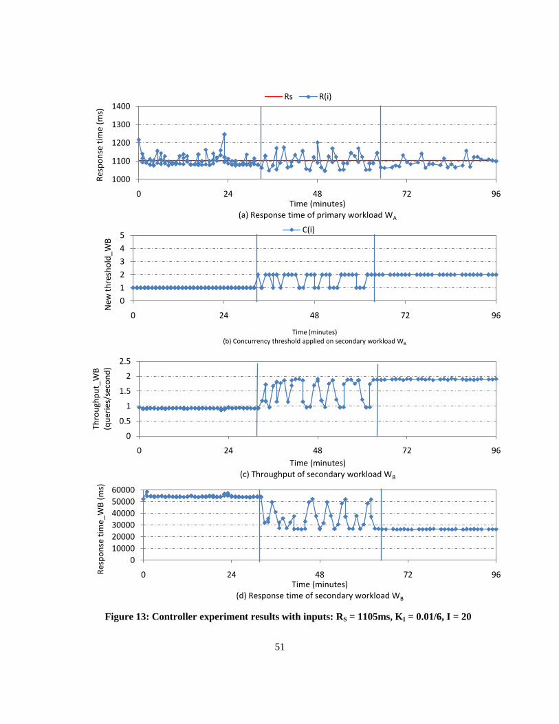
51

Figure 13: Controller experiment results with inputs: RS = 1105ms, KI = 0.01/6, I = 20

1000

1100

1200

1300

1400

0 24 48 72 96

Res

po

nse

tim

e (m

s)

Time (minutes)(a) Response time of primary workload WA

Rs R(i)

0

1

2

3

4

5

0 24 48 72 96

New

th

resh

old

_WB

Time (minutes)(b) Concurrency threshold applied on secondary workload WB

C(i)

0

0.5

1

1.5

2

2.5

0 24 48 72 96

Thro

ugh

pu

t_W

B

(qu

erie

s/se

con

d)

Time (minutes)(c) Throughput of secondary workload WB

0

10000

20000

30000

40000

50000

60000

0 24 48 72 96Res

po

nse

tim

e_W

B (

ms)

Time (minutes)(d) Response time of secondary workload WB

52

4.7.3 Conclusion

All the experiments in this section show that the controller can dynamically adapt to changes in the

workload appropriately. When the workload changes, the controller measures the change through the

response time average R(i) as the response time average of the primary workload changes due to a

change in CPU utilization in the system. This results in error when the controller compares the

response time average R(i) with the response time objective RS. As a result, the controller makes

appropriate changes to the concurrency threshold C(i) on the secondary workload, thereby regulating

the number of secondary workload queries executing in the system so that response time average R(i)

of the primary workload is directed towards objective RS. There were no performance problems of

overshoot and oscillation due to a change in the workload.

These experiments also show that when a response time objective RS does not correspond to a

concurrency threshold, the controller toggles between two thresholds, between which the objective

exists. This results in variant response times for the primary workload without achieving the objective

but only keeping the overall response time average over a larger interval at the objective RS.

Moreover, the fact that the concurrency threshold on the secondary workload is applied variably, it

may not be an attractive behavior of the controller. This shows that the response times of the primary

workload cannot be achieved at a finer granularity and therefore, workload control through

concurrency threshold is a coarse form of control. However, it is to be noted that the more secondary

workload classes there are to control, the more granularity we achieve in controlling the response

times of the primary workload.

4.8 Controller Parameter Tuning and Discussion

In this section, we present the controller experiments with poorly tuned input parameters, controller

constant KI and control interval I. The purpose of these experiments is to show the performance

problems involved when the controller constant KI and control interval I are poorly set for the

controller. We then discuss how to go about choosing appropriate values for KI and I by manual

tuning, based on trial and error. We end this section by giving some pointers to cut down manual

tuning.

53

4.8.1 Controller Experiment 8: Performance Problem with Small Controller Constant KI

We repeated Controller Experiment 1 (in Section 4.5) with smaller controller constant KI of value

0.001 instead of 0.01. The purpose of this experiment is to show how the controller performs if KI is

too small. We perform this experiment with a lower KI of value of 0.001 on response time objective

of 1082 ms from the no-CPU-contention environment. As explained earlier, we expect a low KI of

value 0.001 to work, but at the expense of slowing the controller in converging onto the expected

concurrency threshold 2.

Figure 14 shows the results of this experiment. The controller output graph (in Figure 14(b))

shows that the controller output C(i) reaches the expected threshold 2 in 3000 seconds (75 control

steps, each after an interval of 40 seconds), which is nearly 10 times that of Controller

Experiment 1. Correspondingly, the response time average R(i) (in Figure 14(a)) also reaches the

response time objective 1082 ms. The minor oscillations (step-downs) observed in C(i) in

Experiment 1 are also visibly reduced.

This result shows that if the controller constant KI is too small, then the controller takes a long time

to converge on the response time objective RS. The reason is that if we reduce KI by 10 times, the

controller takes control steps that are 10 times smaller in size. This makes the controller 10 times

slower in responding to errors. Hence, the convergence time of the controller is increased by 10 times.

We may increase the convergence time by reducing the control interval I. However, with the low

arrival rate of the primary workload queries, there can be significant variance in the response time

measurements of the primary workload and can result in the performance problem of oscillation,

which we will be discussing about in Section 4.8.3.

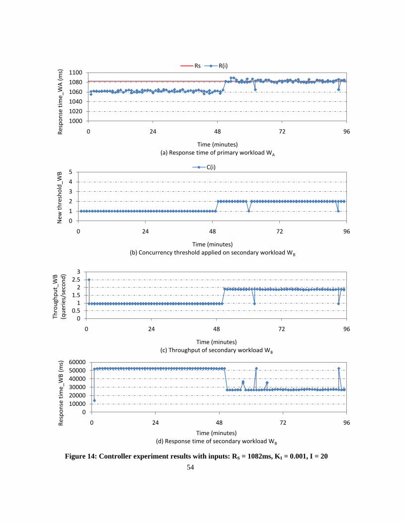
54

Figure 14: Controller experiment results with inputs: RS = 1082ms, KI = 0.001, I = 20

1000

1020

1040

1060

1080

1100

0 24 48 72 96Res

po

nse

tim

e_W

A (

ms)

Time (minutes)(a) Response time of primary workload WA

Rs R(i)

0

1

2

3

4

5

0 24 48 72 96

New

th

resh

old

_WB

Time (minutes)(b) Concurrency threshold applied on secondary workload WB

C(i)

00.5

11.5

22.5

3

0 24 48 72 96

Thro

ugh

pu

t_W

B

(qu

erie

s/se

con

d)

Time (minutes)(c) Throughput of secondary workload WB

0

10000

20000

30000

40000

50000

60000

0 24 48 72 96Res

po

nse

tim

e_W

B (

ms)

Time (minutes)(d) Response time of secondary workload WB

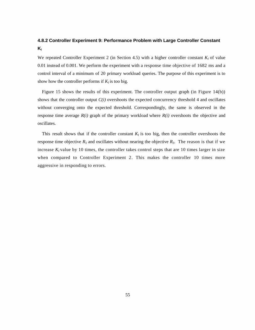
55

4.8.2 Controller Experiment 9: Performance Problem with Large Controller Constant

KI

We repeated Controller Experiment 2 (in Section 4.5) with a higher controller constant KI of value

0.01 instead of 0.001. We perform the experiment with a response time objective of 1682 ms and a

control interval of a minimum of 20 primary workload queries. The purpose of this experiment is to

show how the controller performs if KI is too big.

Figure 15 shows the results of this experiment. The controller output graph (in Figure 14(b))

shows that the controller output C(i) overshoots the expected concurrency threshold 4 and oscillates

without converging onto the expected threshold. Correspondingly, the same is observed in the

response time average R(i) graph of the primary workload where R(i) overshoots the objective and

oscillates.

This result shows that if the controller constant KI is too big, then the controller overshoots the

response time objective RS and oscillates without nearing the objective RS. The reason is that if we

increase KI value by 10 times, the controller takes control steps that are 10 times larger in size

when compared to Controller Experiment 2. This makes the controller 10 times more

aggressive in responding to errors.

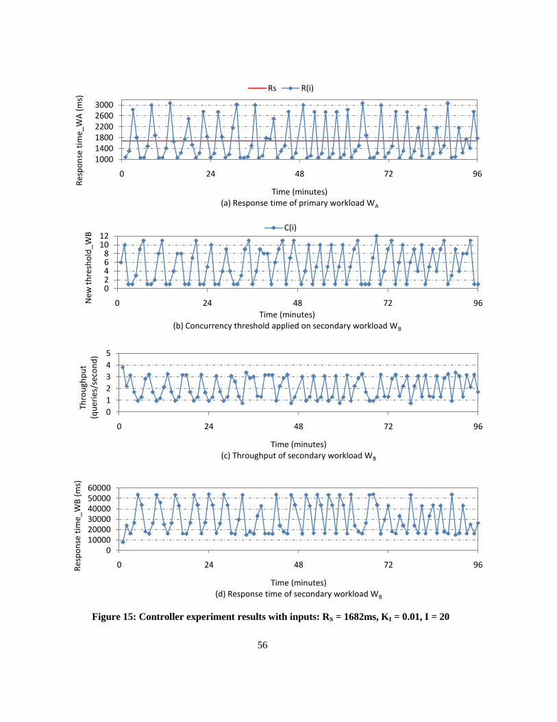
56

Figure 15: Controller experiment results with inputs: RS = 1682ms, KI = 0.01, I = 20

100014001800220026003000

0 24 48 72 96

Res

po

nse

tim

e_W

A (

ms)

Time (minutes)(a) Response time of primary workload WA

Rs R(i)

02468

1012

0 24 48 72 96New

th

resh

old

_WB

Time (minutes)(b) Concurrency threshold applied on secondary workload WB

C(i)

0

1

2

3

4

5

0 24 48 72 96

Thro

ugh

pu

t (q

uer

ies/

seco

nd

)

Time (minutes)(c) Throughput of secondary workload WB

0100002000030000400005000060000

0 24 48 72 96Res

po

nse

tim

e_W

B (

ms)

Time (minutes)(d) Response time of secondary workload WB

57

4.8.3 Controller Experiment 10: Performance Problem with improper Control Interval I

We repeat Controller Experiment 2 (in Section 4.5) with a smaller control interval I of a minimum of

20 primary workload queries instead of a minimum of 40 primary workload queries. We perform the

experiment with a response time objective of 1682 ms and a controller constant KI of 0.001. The

purpose of this experiment is to show how the input parameter I affects the performance of the

controller.

Figure 16 shows the results of this experiment. The new threshold graph (Figure 16(b)) shows that

the controller output C(i) smoothly climbs to the expected concurrency threshold 4 in 280 seconds (7

control steps, each after an interval of 40 seconds), which is half of that of Controller Experiment 2,

but oscillates largely between concurrency thresholds 3 and 4 and does not stabilize on threshold 4.

This is due to high variance in the response time measurements at threshold 4.

This result shows that the number of primary workload queries in a control interval I affect the

performance of the controller. Provided with a proper controller constant KI, the controller output C(i)

reaches the expected concurrency threshold without overshoot, but oscillates around the expected

threshold and does not settle on the threshold. The reason is for this is that if there are fewer queries

in a control interval I, the controller is more prone to being affected by the variance in the response

time average measurements. Having more primary workload queries in a control interval I smoothes

out the variance as the response time average measurements is averaged over more queries.

58

Figure 16: Controller experiment results with inputs: RS = 1682ms, KI = 0.001, I = 20

1000

1400

1800

2200

2600

3000

0 24 48 72 96Res

po

nse

tim

e_W

A (

ms)

Time (minutes)(a) Response time of primary workload WA

Rs R(i)

0123456

0 24 48 72 96

New

th

resh

old

_WB

Time (minutes)(b) Concurrency threshold applied on secondary workload WB

C(i)

0123456

0 24 48 72 96

Thro

ugh

pu

t (q

uer

ies/

seco

nd

)

Time (minutes)(c) Throughput of secondary workload WB

0100002000030000400005000060000

0 24 48 72 96

Res

po

nse

tim

e_W

B (

ms)

Time (minutes)(d) Response time of secondary workload WB

59

4.8.4 Tuning Controller Constant KI and Control Interval I Experimentally

Inappropriate values for KI and I can result in performance problems of overshoot, oscillation and

longer convergence times. Therefore, proper tuning is necessary for KI and I.

By tuning the parameters KI and I, we are able to control the aggressiveness of the controller.

Tuning KI changes the size of the control steps taken by the controller to move from one threshold to

another and therefore, by tuning KI, we are able to control the controller’s sensitivity to error. Tuning

I changes the number of control decisions per unit time, thereby changing the time span over which

the response time measurements of the primary workload are averaged and therefore, by tuning I, we

are able to control the controller’s sensitivity to variance.

The following is how to deal with a performance problem of overshoot and oscillation by tuning KI

and I.

1. If the controller overshoots the response time objective RS, oscillates and does not near the

objective, as in Controller Experiment 9, then this problem is due to a high KI and therefore,

KI needs to be decreased.

2. If the controller converges onto the objective RS but doesn’t stay on RS and oscillates, as in

Controller Experiment 10, then this problem is due to significant variance in the response

time measurements of the primary workload and therefore, I needs to be increased to

minimize variance.

The performance problem of longer convergence time, where the controller takes a significant

amount of time to converge onto the objective RS, as in Controller Experiment 8, is due to a low KI

and therefore, KI needs to be increased. It is to be noted that decreasing I can also increase the

convergence time.

4.8.5 Choosing Controller Constant KI

In all the controller experiments in this thesis, we used values for controller constant KI that were

obtained experimentally, based on trial and error. We used a KI of value 0.01 for response time

objectives from the no-CPU-contention environment and a KI of value 0.001 for response time

objectives from the CPU-contention environment. Practically, it is not realistic to perform manual

60

tuning of KI without having any pointers to starts from. Therefore, we discuss some possible ways to

reduce manual tuning in this section.

In the previous chapter, we defined the controller constant KI to be the amount by which the

controller should manipulate the concurrency threshold for a unit amount of error in the response time

of the primary workload.

𝐾𝐼 =𝐶 𝑖 − 𝐶(𝑖 − 1)

𝐸(𝑖)

Considering the slopes of trends from the response time curve (in Figure 2(a)) in the workload

characterization experiment, for response time objectives from the no-CPU-contention environment,

we know that we want the controller to have the granularity to change the concurrency threshold at

most by 1 if the error is of value 23 ms. Therefore, we want KI of value 0.04 in no-CPU-contention

environment.

𝐾𝐼 =1

23= 0.04

Similarly, for response time objectives from the CPU-contention environment, we know that we

the controller to change the concurrency threshold by 1 if the error is of value 225 ms. Therefore, we

want KI of value 0.004 in CPU-contention environment.

𝐾𝐼 =1

225= 0.004

These values 0.04 and 0.004 for KI are the highest that KI should be in each environment, making

the controller to adjust for response time error in a single control step, which may result in an

aggressive controller.

From the properly tuned controller experiments in Section 4.5, Controller Experiment 1 took 6

control steps to move from threshold 1 to threshold 2 in the beginning of the experiment in no-CPU-

contention environment. Therefore, the KI value that works well in that experiment should be 0.0067.

𝐾𝐼 =0.04

6= 0.0067

When this value is rounded off, it is equal to 0.01, which is what we used in Controller Experiment

1.

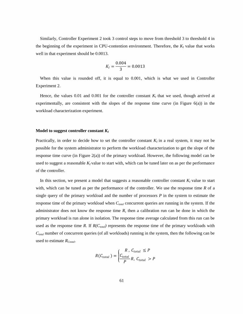
61

Similarly, Controller Experiment 2 took 3 control steps to move from threshold 3 to threshold 4 in

the beginning of the experiment in CPU-contention environment. Therefore, the KI value that works

well in that experiment should be 0.0013.

𝐾𝐼 =0.004

3= 0.0013

When this value is rounded off, it is equal to 0.001, which is what we used in Controller

Experiment 2.

Hence, the values 0.01 and 0.001 for the controller constant KI that we used, though arrived at

experimentally, are consistent with the slopes of the response time curve (in Figure 6(a)) in the

workload characterization experiment.

Model to suggest controller constant KI

Practically, in order to decide how to set the controller constant KI in a real system, it may not be

possible for the system administrator to perform the workload characterization to get the slope of the

response time curve (in Figure 2(a)) of the primary workload. However, the following model can be

used to suggest a reasonable KI value to start with, which can be tuned later on as per the performance

of the controller.

In this section, we present a model that suggests a reasonable controller constant KI value to start

with, which can be tuned as per the performance of the controller. We use the response time R of a

single query of the primary workload and the number of processors P in the system to estimate the

response time of the primary workload when Ctotal concurrent queries are running in the system. If the

administrator does not know the response time R, then a calibration run can be done in which the

primary workload is run alone in isolation. The response time average calculated from this run can be

used as the response time R. If R(Ctotal) represents the response time of the primary workloads with

Ctotal number of concurrent queries (of all workloads) running in the system, then the following can be

used to estimate RCtotal.

𝑅(𝐶𝑡𝑜𝑡𝑎𝑙 ) =

𝑅 , 𝐶𝑡𝑜𝑡𝑎𝑙 ≤ 𝑃𝐶𝑡𝑜𝑡𝑎𝑙

𝑃𝑅, 𝐶𝑡𝑜𝑡𝑎𝑙 > 𝑃

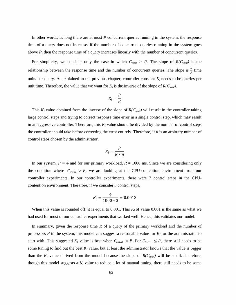
62

In other words, as long there are at most P concurrent queries running in the system, the response

time of a query does not increase. If the number of concurrent queries running in the system goes

above P, then the response time of a query increases linearly with the number of concurrent queries.

For simplicity, we consider only the case in which Ctotal > P. The slope of R(Ctotal) is the

relationship between the response time and the number of concurrent queries. The slope is 𝑅

𝑃 time

units per query. As explained in the previous chapter, controller constant KI needs to be queries per

unit time. Therefore, the value that we want for KI is the inverse of the slope of R(Ctotal).

𝐾𝐼 =𝑃

𝑅

This KI value obtained from the inverse of the slope of R(Ctotal) will result in the controller taking

large control steps and trying to correct response time error in a single control step, which may result

in an aggressive controller. Therefore, this KI value should be divided by the number of control steps

the controller should take before correcting the error entirely. Therefore, if n is an arbitrary number of

control steps chosen by the administrator,

𝐾𝐼 =𝑃

𝑅 ∗ 𝑛

In our system, 𝑃 = 4 and for our primary workload, R = 1000 ms. Since we are considering only

the condition where 𝐶𝑡𝑜𝑡𝑎𝑙 > 𝑃, we are looking at the CPU-contention environment from our

controller experiments. In our controller experiments, there were 3 control steps in the CPU-

contention environment. Therefore, if we consider 3 control steps,

𝐾𝐼 =4

1000 ∗ 3= 0.0013

When this value is rounded off, it is equal to 0.001. This KI of value 0.001 is the same as what we

had used for most of our controller experiments that worked well. Hence, this validates our model.

In summary, given the response time R of a query of the primary workload and the number of

processors P in the system, this model can suggest a reasonable value for KI for the administrator to

start with. This suggested KI value is best when 𝐶𝑡𝑜𝑡𝑎𝑙 > 𝑃. For 𝐶𝑡𝑜𝑡𝑎𝑙 ≤ 𝑃, there still needs to be

some tuning to find out the best KI value, but at least the administrator knows that the value is bigger

than the KI value derived from the model because the slope of R(Ctotal) will be small. Therefore,

though this model suggests a KI value to reduce a lot of manual tuning, there still needs to be some

63

tuning required to find the best controller constant KI, which can be done experimentally based on the

guidelines presented in Section 4.8.4.

4.8.6 Choosing Control interval I

In all the controller experiments, we used arbitrary values for the control interval I. We had to

consider variance in tuning the control interval I because the workloads that we used had a low arrival

rate of queries. In the no-CPU-contention environment, the variance in the response time

measurements was less and hence, we used a smaller control interval of a minimum of 20 primary

workload queries. In the CPU-contention environment, the variance in the response time

measurements was significantly high and in order to smooth out the variance, we used a longer

control interval I of a minimum of 40 primary workload queries.

Practically, the control interval I may not require a lot of tuning because most of the transactional

database workloads in a real system have high arrival rates. Hence, a reasonable control interval can

be easily chosen by the system administrator and the interval will have a good number of queries and

therefore there will not be any significant variance in the response time average measurements. The

same control interval will work for both no-CPU-contention environment and CPU-contention

environment. We examine the feasibility of using our controller on workloads with higher arrival

rates in the next section.

4.9 Workloads with Small Inter-Arrival Time and Small Service Time

Most of the transactional workloads in current DBMSs have a high arrival rate of queries with

sub-second service times. Therefore, we examine the feasibility of achieving response time

objectives for workloads with small service time TS and small inter-arrival time TA.

4.9.1 Effectiveness of Controller on Workloads with Higher Arrival Rate

We use two workload streams WD and WE as shown in Table 7. We use a service time of 200 ms and

an inter-arrival time of 120 ms for the primary workload WD and the secondary workload WE.

64

Therefore, both the workloads together have a CPU utilization of 3.2. We use random service time

TS and random inter-arrival time TA.

Test

Workloads

Workload

Streams 𝑻𝑺 [value (ms), distribution] 𝑻𝑨 [value (ms), distribution]

Primary WD 200, exponential 120, exponential

Secondary WE 200, exponential 120, exponential

Table 7: Test workloads WD and WE configurations

We perform workload characterization as in Experiment 2 of Section 5.4 on workloads WD and WE.

In this experiment, we determine whether admission control on the secondary workload WE is an

effective way to control the response time of the primary workload WD. The result of the experiment

is shown in Figure 16.

Figure 17: Sensitivity of response time average of WD to concurrency threshold on WE

The figure shows that the response time averages of WD increase consistently, starting from

threshold 1. This is because of increase CPU utilization with increase in concurrency threshold on WE.

With exponential service times and exponential inter-arrival times, there may be queries with service

200

250

300

350

400

450

500

1 2 3 4 5 6 7 8 9 10 11

Res

po

nse

tim

e (m

s)

Threshold

WDWD

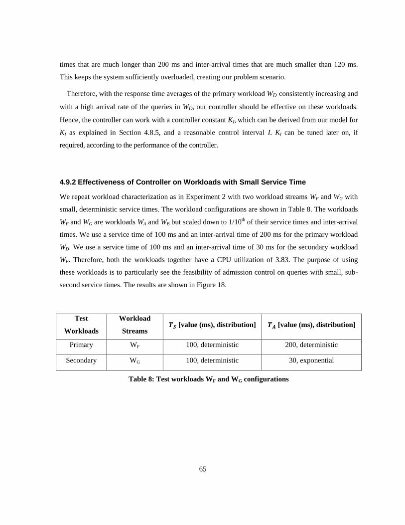
65

times that are much longer than 200 ms and inter-arrival times that are much smaller than 120 ms.

This keeps the system sufficiently overloaded, creating our problem scenario.

Therefore, with the response time averages of the primary workload WD consistently increasing and

with a high arrival rate of the queries in WD, our controller should be effective on these workloads.

Hence, the controller can work with a controller constant KI, which can be derived from our model for

KI as explained in Section 4.8.5, and a reasonable control interval I. KI can be tuned later on, if

required, according to the performance of the controller.

4.9.2 Effectiveness of Controller on Workloads with Small Service Time

We repeat workload characterization as in Experiment 2 with two workload streams WF and WG with

small, deterministic service times. The workload configurations are shown in Table 8. The workloads

WF and WG are workloads WA and WB but scaled down to 1/10th of their service times and inter-arrival

times. We use a service time of 100 ms and an inter-arrival time of 200 ms for the primary workload

WD. We use a service time of 100 ms and an inter-arrival time of 30 ms for the secondary workload

WE. Therefore, both the workloads together have a CPU utilization of 3.83. The purpose of using

these workloads is to particularly see the feasibility of admission control on queries with small, sub-

second service times. The results are shown in Figure 18.

Test

Workloads

Workload

Streams 𝑻𝑺 [value (ms), distribution] 𝑻𝑨 [value (ms), distribution]

Primary WF 100, deterministic 200, deterministic

Secondary WG 100, deterministic 30, exponential

Table 8: Test workloads WF and WG configurations

66

Figure 18: Sensitivity of response time average of WF to concurrency threshold values on WG

The figure shows that the response time averages of WF are not affected by change in concurrency

threshold on WG. This is because the queries of the workloads are too short, probably shorter than the

CPU time slice of the operating system’s scheduler. If we assume that the operating system uses

round robin (RR) scheduling, with the time slice being too big for the very small queries, the RR

scheduler will start to perform as a first-come-first-serve (FCFS) scheduler. Therefore, the context

switches for each query becomes significantly low. Therefore, with increase in concurrency, there is

negligible increase in context switches for each query and therefore, CPU wait time TW for each query

will almost remain the same. In conclusion, the response times of these very small queries do not

increase by increase in the number of concurrent queries in the system. This proves that our

controller’s concurrency threshold control will not be effective for workloads with very small queries.

4.10 Summary

In this chapter, based on all the experiments, we can conclude that our admission controller

has a certain number of advantages and a certain number of disadvantages.

The following are the advantages of the controller:

1. The controller is able to keep the response time average of the primary workload at the

response time objective with minimal performance problems, after careful tuning of input

parameters: controller constant KI and control interval I.

0.0020.0040.0060.0080.00

100.00120.00140.00

1 3 4 7 9

Res

po

nse

tim

e (m

s)

Threshold

WFWF

67

2. The controller, if properly tuned, is able to automatically adjust to changing response time

objective and changing workload conditions without any performance problems.

3. The aggressiveness and the convergence time of the controller can be controlled by

controlling the controller constant KI and the control interval I.

The following are the disadvantages of the controller:

1. Tuning the controller constant KI and the control interval I may be difficult in practice.

2. If the number of secondary workload classes to control is less, the controller’s admission

control can be a coarse form of control to achieve response time objectives.

3. The controller is not effective for workloads with very small queries because their CPU wait

time TW is not affected by concurrency threshold. Hence, the controller’s admission control

does not affect the response times of very small queries.

68

Chapter 5

Conclusion

In this thesis, we study achieving performance objectives for a primary workload in DBMSs. We

focus on how to use feedback-based admission differentiation to achieve the performance objectives.

We use admission control on secondary workloads to achieve objectives for the primary workload.

The amount of admission control to be applied is decided on the current performance of the primary

workload and how far it is from the objective.

We propose a general architectural framework for feedback-based admission differentiation. It

consists of three components: workload classifier, workload monitor and adaptive admission

controller. The workload classifier identifies and groups the incoming queries into workloads

according to their source or type. The workload monitor is concerned with providing feedback about

the workloads to the adaptive admission controller by continuously collecting performance

information. The adaptive admission controller calculates and implements admission control on the

secondary workload. The adaptive admission controller has two sub-components, namely an advisor

and effector. The advisor reads the performance information of the primary workload, compares the

information to the workload’s objective and calculates the amount of admission control to be applied

on the secondary workload. The amount of admission control to be applied is determined by using

fundamentals from control theory. Effector implements the admission control calculated on the

secondary workload.

In order to prove the effectiveness of feedback-based admission differentiation, we implemented all

the components in a commercial DBMS, DB2. We achieve response time objectives for the primary

workload by applying admission control in the form of applying a concurrency threshold to the

secondary workload.

We show that the adaptive admission controller is able to regulate the response time average of the

primary workload towards the workload’s response time objective by controlling the concurrency

threshold on the secondary workload, given an appropriate controller constant KI and control interval

I.

69

We evaluate the controller in different scenarios in which the response time objective or the

workload changes. The experiments in which response time objective changes show that the

controller can achieve both the objectives and handle the change effectively without oscillation. The

experiments in which workload changes show that the controller can dynamically achieve the

objective through the workload changes, without oscillation as well.

We show how controller constant KI and control interval I affect the performance of the controller.

The experiments show that we can control the aggressiveness of the controller by changing KI and I.

We also show the feasibility of the using the controller for workloads with a high arrival rate and

sub-second service times. The experiments showed a limitation of the controller that it is not effective

on workloads with very small queries because the queries are too small and therefore, the context

switching for each query does not increase with increase in concurrency in the system. Therefore, the

controller’s concurrency threshold control on the secondary workload (with small queries) do not

affect the response times of the primary workload (with very small queries).

In conclusion, a properly tuned adaptive admission controller is able to achieve response time

objectives for an important, primary workload by applying concurrency threshold control on the less

important, secondary workload, as long as the workload do not consist of very small queries. Hence,

the controller experiments in this thesis show that it is feasible to use feedback-based admission

differentiation to achieve performance objectives for a primary workload in a DBMS.

Having shown the effectiveness of the controller, it will be interesting to see the following as future

work:

1. Develop a method to auto-tune the controller constant KI. In this thesis, we showed a model

to derive a value for controller constant KI with the response time R and the number of

processors P. Though the derived value saves the administrator from a lot of tuning, it may

still require a bit of tuning to obtain the best KI value. Hence, it is necessary to develop a

well-defined process to tune KI automatically to avoid any manual tuning.

2. Enhance our feedback-based admission differentiation framework to achieve per-class

performance objectives for multiple workload classes. Achieving multiple performance

objectives is complicated by the interdependence between workload classes. Achieving

performance objective of one class affects the performance of the other classes. Therefore, we

70

need to develop a well-defined function to manage the objectives of all the workload classes

collectively.

3. Improve the objective specification for the architectural framework to include business

importance of the workload classes. In this thesis, we assumed the business importance of the

workloads and we designed the architectural framework to allow specifying the performance

objectives as values. There is no method to specify business importance of a workload class

which can define how important it is to achieve the objective of the class relative to other

workload classes. Therefore, integrating importance of workload classes along with their

performance objectives will be a good improvement to add to the framework.

4. Test the controller for achieving performance objectives of other metrics. For example, if

applying concurrency threshold on the secondary workloads affects the throughput of the

primary workload, then the controller can achieve throughput objectives of the primary

workload.

5. Investigate if the controller can be used on a wider range of workloads and not just read-only

transactional workloads.

71

References

[1] IBM Canada. Introduction to DB2 9.5 Workload Management. 2007.

[2] J. L. Hellerstein, Y. Diao, S. Parekh and D. M. Tilbury. Feedback Control of Computing Systems.

John Wiley & Sons, 2004.

[3] S. Krompass, A. Scholz, M. Albutiu, H. Kuno, J. Wiener, U. Dayal and A. Kemper. Quality of

Service-Enabled Management of Database Workloads. IEEE Data Engineering Bulletin, Special

Issue on Testing and Tuning of Database Systems, volume 31, issue 1, 2008.

[4] A. Moenkeberg and G. Weikum. Conflict-driven load control for the avoidance of data-contention

thrashing. In Proceedings of the Seventh International Conference on Data Engineering, pages 632-

639, 1991.

[5] M. J. Carey, S. Krishnamurthi and M. Livny. Load control for locking: The "half-and-half''

approach. In PODS '90: Proceedings of the Ninth ACM SIGACT-SIGMOD-SIGART Symposium on

Principles of Database Systems, Nashville, Tennessee, United States, pages 72-84, 1990.

[6] H. Heiss and R. Wagner. Adaptive load control in transaction processing systems. In VLDB '91:

Proceedings of the 17th International Conference on very Large Data Bases, pages 47-54, 1991.

[7] K.D. Kang, Sang H. Son and John A. Stankovic. Service differentiation in real-time main memory

databases. In ISORC '02: Proceedings of the Fifth IEEE International Symposium on Object-Oriented

Real-Time Distributed Computing, page 119, 2002.

[8] S. Elnikety, E. Nahum, J. Tracey and W. Zwaenepoel. A method for transparent admission control

and request scheduling in e-commerce web sites. In WWW '04: Proceedings of the 13th International

Conference on World Wide Web, New York, NY, USA, pages 276-286, 2004.

[9] B. Schroeder, M. Harchol-Balter, A. Iyengar, E. Nahum and A. Wierman. How to determine a

good multi-programming level for external scheduling. In ICDE '06: Proceedings of the 22nd

International Conference on Data Engineering, page 60, 2006.

[10] K. D. Kang, P. H. Sin and D. K. Shin. A feedback-based approach for data contention control. In

Symposium of Information and Communication Technology, Raleigh, North Carolina, August, 2004.

[11] K. P. Brown, M. Mehta, M. J. Carey and M. Livny. Towards automated performance tuning for

complex workloads. In VLDB '94: Proceedings of the 20th International Conference on very Large

Data Bases, pages 72-84, 1994.

[12] H. Pang, M. J. Carey and M. Livny. Multiclass Query Scheduling in Real-Time Database

Systems.IEEE Trans.on Knowl.and Data Eng., volume 7, issue 4, pages 533-551, 1995.

[13] N. Bhatti and R. Friedrich. Web server support for tiered services. IEEE Network, volume 13,

issue 5, pages 64-71, September/October, 1999.

72

[14] T. F. Abdelzaher, K. G. Shin and N. Bhatti. Performance Guarantees for Web Server End-

Systems: A Control-Theoretical Approach. IEEE Trans. Parallel Distrib. Syst., volume 13, issue 1,

pages 80-96, 2002.

[15] Chenyang Lu, John A. Stankovic, Sang H. Son and Gang Tao. Real Time Systems - Feedback

Control Real-Time Scheduling: Framework, Modeling, and Algorithms. In Journal of Real-Time

Systems, Special Issue on Control-Theoretical Approaches in Real-Time Computing, volume 23, issue

1, page 85, 2002.

[16] J. Huang, J. A. Stankovic, K. Ramamritham and D. Towsley. On using priority inheritance in

real-time databases. Technical Report, COINS TR 90-121, Department of Computer and Information

Science, University of Massachusetts, Amherst, MA, USA, 1990.

[17] J. Almeida, M. Dabu, A. Manikutty and P. Cao. Providing Differentiated Levels of Service in

Web Content Hosting. In Proceedings of the Workshop on Internet Server Performance, pages 91-

102, 1998.

[18] HP. HP NeoView Workload Management Services Guide. August, 2007.

[19] Teradata. Teradata Dynamic Workload Manager User Guide. September, 2006.

[20] R. Mistry. Microsoft SQL Server 2008 Management and Administration. Carmel, IN, USA:

SAMS, 2009.

[21] IBM. DB2 Workload Manager for Linux, Unix, and Windows. Riverton, NJ, USA: IBM Corp,

2008.