Achieving High Lifetime and Low Delay in

Very Large Sensors Networks using Mobile Sinks

Technical Report No. 385/11

Wint Yi Poe, Michael Beck, Jens B. Schmitt

Distributed Computer Systems Lab (DISCO), University of Kaiserslautern, Germany

Abstract. For smaller scale wireless sensor networks (WSN) it has beenclearly shown that a single mobile sink can be very bene�cial with re-spect to the network lifetime. Yet, how to plan the trajectories of many

mobile sinks in very large WSNs in order to simultaneously achieve life-

time and delay goals has not been treated so far. In this report, we delveinto this di�cult problem and propose a heuristic framework using multi-ple orbits for the sinks' trajectories. The framework is carefully designedbased on geometric arguments to achieve both, high lifetime and lowdelay. In simulations, we compare two di�erent instances of our frame-work, one conceived based on a load balancing argument and one basedon a distance minimization argument, with a set of di�erent competitorsspanning from statically placed sinks to battery-state aware strategies.We �nd our heuristics to perform very favorably: both instances out-perform the competitors in both, lifetime and delay. Furthermore, andprobably even more importantly, the heuristic, while keeping its gooddelay and lifetime performance, scales well with an increasing number ofsinks.

Keywords.Very large WSNs, Sink Trajectory, Worst-Case Delay, Life-time.

1 Introduction

There is a growing trend for ever larger wireless sensor networks (WSN) consist-ing of thousands or tens of thousands of sensor nodes. For example, the WSNbuilt by the GreenOrbs project at Zhejiang Forestry University for forest surveil-lance [10] employs 1000+ nodes. We believe this trend will continue and thusscalability plays a crucial role in all protocols and mechanisms for WSNs. An-other trend in many modern WSN applications is the sensitivity to the delayfor the information transfer from sensors to sinks. In particular, WSNs are acentral part of the vision of cyber-physical systems and as these are basicallyclosed-loop systems many WSN applications will have to operate under stringenttiming requirements. Hence, information transfer delays need to be controlled.On the other hand, since most WSNs are still based on battery-operated nodes,energy-e�ciency clearly remains another premier goal in order to keep networklifetime high. How to achieve a lifetime prolongation by using mobile sink(s) tocollect the data of a WSNs has already been investigated in many works (e.g.,[12, 2, 29, 24]). All of these leverage on the e�ect that the burden of being close

to a sink is shared over time among all the nodes in the �eld. This alleviates thetypical hot-spot problem, where nodes near the sink drain their battery muchfaster than others since they have to relay many data packets for other nodes.However, by using mobile sinks, in general, the information transfer delay fromsensors to sinks increases. This is simply due to the fact that there is alwaysa delay-optimal placement of the sinks and leaving it the message transfer de-lay becomes worse. This con�ict between lifetime and delay shows that thesetwo goals have to be carefully traded o� against each other when planning thetrajectories of multiple mobile sinks.

The contributions of our report are:

� To the best of our knowledge, we are the �rst to tackle the trajectory plan-ning problem for multiple mobile sinks in very large WSNs under lifetimeand delay goals.

� We derive a heuristic framework that keeps up its delay and lifetime per-formance in very large WSNs as long as a constant node to sink ratio isretained. (→Section 4)

� A thorough simulative investigation and comprehensive comparison with al-ternative approaches inspired by literature is presented. (→Section 5)

Our work is based on using multiple orbital trajectories for the mobile sinksand segment the sensor �eld into a so-called polar grid. In each orbit the sinksare moved synchronously (e.g., once a day), following a slow mobility approach[13]. For the case of very large WSNs with many mobile sinks (say hundreds)this n-orbit model generalizes recent previous work of ours using only 2 orbits[19]. While we base on this work with respect to giving the problem a geomet-ric interpretation, we remark that the n-orbit case is signi�cantly harder. Mostseverely, the distribution of K sinks over n orbits leads to a combinatorial ex-plosion of the search space for the values of K that we require in very largeWSNs. Similarly, the optimal choice of the number of orbits n as well as thesizing of their radii become very di�cult questions. We address these questionswith a heuristic framework. It is built on a geometric reduction of the problem,where the two performance characteristics, delay and lifetime, are amalgamatedinto minimizing the Euclidean distance between nodes and sinks. The intuitionbehind this is that both, delay and lifetime, bene�t from nodes being closer interms of Euclidean distance to their assigned sinks.

2 Related Work

In literature, a considerable number of works advocate for using a single ormultiple mobile sinks [2, 3, 4, 23, 12, 14, 16, 29, 5, 19, 27, 28, 6, 24, 9]. Themajority of these deal with single sinks [2, 12, 16, 29, 17, 27, 24, 30, 9] and allof them focus on prolonging lifetimes. The e�ects on information transfer delayare either completely neglected or simply observed without taking actions toestablish delay as an objective of equal importance to lifetime maximization.Clearly, the single mobile sink studies were not conceived with very large WSNsin mind; however, even the works on multiple mobile sinks usually considered arather low number of sinks and nodes and did not investigate the scalability ofthe proposed mechanisms. In our work, we target very large WSNs and strive for

high lifetime and low delay simultaneously, which sets us apart from the currentstate-of-the-art. Having said that, many of the previous works have inspired ourwork and we discuss them now separately:

Sink trajectories can be categorized into random, state-dependent, and pre-de�ned. Usage of a random trajectory can, e.g., be found in [4] where mobilesinks perform a random walk and collect the data from the sensors of theirassigned clusters trying to achieve a load balancing and lifetime maximization.

Recently, [2, 27, 16] address state-dependent sink mobility for maximizingthe lifetime of WSNs. In their approaches, the sink trajectory is a function of aparticular network variable, such as, e.g., the state of nodes' batteries. Thoughthe lifetime performance of such trajectories is good, the methods assume knowl-edge of global and dynamic information for determining the optimal paths andsojourn times, which is a strong assumption in very large WSNs.

[6, 26] propose a prede�ned single sink trajectory independent of any networkstate such that the sink appears on the same path periodically. [15] also pro-poses a geometrically motivated pre-de�ned trajectory for multiple sinks wherethe sinks move on the perimeters of a hexagonal tiling. This is shown to bebene�cial for lifetime prolongation. Like us they require no a priori knowledgeof node locations which is desirable for very large WSNs, yet they do not con-sider delay performance. In contrast to a periodical movement, the work in [11]proposes a prede�ned sink trajectory where the sink only appears once at eachposition along the trajectory. The author studied the improvement of lifetimeprolongation by using a joint sink mobility and routing scheme similar to [17].

In our work, we tackle the problem of �nding good trajectories for multiplemobile sinks such that we keep the maximum message delay low and still achievea long lifetime. So, delay and energy are traded o� against each other. Alongsimilar lines, [27] optimizes this trade-o�, too, designing a trajectory for a �datamule� which collects the data from each sensor node directly [23]. Yet, the datamule approach incurs long latencies and is generally not applicable in delay-sensitive WSNs. In [29, 17, 11], the movement of a sink is abstracted as a sequenceof a static sink placements assuming that the time scale of sink mobility is muchlarger than that of data delivery; we also follow this assumption of slow mobility(as it has been coined in [13]) in our work.

3 Network Model and Problem Statement

Let V be the set of sensor nodes with |V | = N ; S is the set of sinks with|S| = K. For both, N and K we assume large scales with N being on theorder of thousands and K up to the order of hundreds. The reachability betweennodes is modelled as a directed graph, G = (V, E), where V = V ∪ S. For alla, b ∈ V, the edge (a, b) ∈ E exists if and only if a and b are within a disc-basedtransmission range rtx. The sensor �eld is assumed to be a circular area withradius R.

3.1 The Nodes

The nodes are i.i.d. uniformly distributed over the sensor �eld. We assume thenode density (governed by the parameters R and N) to be high enough to ensure

connectivity with high probability (see also Section 5.4). The nodes are homo-geneous with respect to their initial energy E and their transmission range rtx.Also, the costs for sending and receiving messages do not di�er from node tonode. The amount of data produced by each of the nodes is the same and followsthe same tra�c pattern, e.g., a periodic data generation. The energy consump-tion for operations other than receiving or transmitting can be neglected, sincefor homogenous nodes they consume the same amount of energy. The nodes arestationary and use multi-hop-communication to send their data to their assignedsink. This means the routing topology is actually a forest of sink trees embeddedin the reachability graph G. The assignment of nodes to sinks is further discussedin Section 4.

3.2 The Sinks

The sinks are assumed to have no energy constraints. We assume that the sinks'movement is synchronous, i.e., all sinks move at the same time. Further, sinkmovement takes places on relatively long time-scales (e.g., once a day), muchlarger than the time-scale of the message transfer delay from sensors to sinks(e.g., on the order of seconds). Therefore, we neglect the time periods when thesinks are actually moving (or being moved) and the sink mobility is abstractedas a sequence of sinks' locations. At each location the sinks stay for an equalamount of time, further on called epochs. In particular, we also assume that alldata is �ushed from the WSN before a sink movement takes place, i.e., there isno data dependency between epochs.

3.3 The Problem Statement

In this setting, we want to simultaneously achieve a low information transferdelay and a long lifetime. Here, we de�ne lifetime as the time until the �rstnode of the network �dies�, i.e., its battery is depleted. For the delay, we considerthe worst-case message transfer delay for the whole network. To that end, weuse sensor network calculus [20] to compute the worst-case delays for each datastream from a node to its sinks and take the largest of these worst-case delaysas the worst-case delay for the whole network.

To solve this dual-objective problem one basically has to answer three ques-tions in each epoch:

1. Sink Trajectories: where should the sinks be positioned?2. Sink Selection: which sink does a node choose to send its data to?3. Sink-Tree Routing: which route is the data sent to the sink?

In this report, we focus on the planning of the sink trajectories and �hard-code�the other two questions: for sink selection, each node chooses its nearest sink withrespect to Euclidean distance (within the same orbit, more details are given inSection 4); for the routing we assume shortest path routing in the reachabilitygraph G, mainly because it is a frequent case. Yet, even under these restrictions,the problem is still a very hard one (even strong reductions of it are NP-hard,see also [19] for a discussion of this). The main complexity has its roots in thecon�icting objectives delay and lifetime. The end-to-end delay, as well as the

energy consumption, is dependent on the path between nodes and their sink, aswell as any other path interfering with this one. Hence there is a dependencystructure between the end-to-end delays which is very hard to untangle.

4 Heuristic Framework

In this section, we present our heuristic framework for planning the sink trajec-tories in very large WSNs with delay and lifetime goals. Due to the complexityof the problem, we reduce it to a geometric problem. This abstraction is justi-�able by the large scale of the WSN as we target it in our work. The rationalebehind it is that the delay (mainly governed by the number of hops) needed toreach a sink is proportional to the Euclidean distance from the nodes to theirsinks. On the other hand, per epoch, we divide the network area in a number ofcells (using a polar grid segmentation of the circular sensor �eld), correspond-ing to the number of sinks. In each epoch, each node is assigned to the sinkof its currently corresponding cell. Thus, we can abstract the load assigned toa single sink as the area of its cell. This geometric interpretation of load anddelay is instrumental in constructing good sink trajectories, because instead ofcomplex delay and energy functions we can now formulate the problem in termsof the size of cells and Euclidean distances between nodes and sinks, which areconsiderably simpler measures.

4.1 Orbital Sink Trajectories

Table 1. Notations for the orbit model.

R Radius of the network area.

N Number of nodes used.

K Number of sinks used.

L Leftover sinks.

n Number of orbits used.

Ki; i ∈ {1, . . . , n} Number of sinks placed in the i-th orbit.

Ri; i ∈ {1, . . . , n} Radius of the i-th circle,constructing the polar grid.

di; i ∈ {1, . . . , n} Maximal distance of one point in a cellof the i-th orbit, to the corresponding sink.

ai; i ∈ {1, . . . , n} The area of one cell in the i-th orbit.

θ Movement angle of the sinks between epochs.

γ ∈ [1, 2] For γ = 1 we get the MD-approach,for γ = 2 the EA-approach.

Our heuristic framework is based on an orbital model for the sink trajec-tories in order to achieve a small distance between nodes and their sinks, aswell as a balanced division of the network area into cells [19]. In a nutshell, itworks like this: we conceive several circles around the center of the sensor �eld,

with di�erent radii, called orbits; the sinks are placed on these orbits with reg-ular interspaces and revolve around the center, like satellites move around theearth (see Figure 1). For a more detailed presentation of this n-orbit model, weintroduce some de�nitions and notations (see also Table 1):

� We call the innermost orbit the �rst orbit and the outermost orbit the lastor n-th orbit.

� By a sink distribution we refer to how many sinks are placed in each of theorbits; we denote the number of sinks placed in the i-th orbit by Ki.

� The orbits and their sinks divide the network area in a polar grid as illus-trated in Figure 1. The cells within the same orbit have the same shape andsize. The sinks are located in the center of their cells, such that they mini-mize the maximal Euclidean distance of any point of this cell to themselves.This center can be calculated by replacing the cell by a trapezoid (or trian-gle, in the case of the �rst orbit) sharing the same corner points as the celland determining the center of the minimal enclosing circle of this trapezoid.A formal proof for the correctness of this intuitive statement can be foundin [18].

� The polar grid consists of n concentric circles segmenting the sensor �eldinto circular segments as well as ring segments. By Ri (i ∈ {1, . . . , n}) wedenote the radii of the concentric circles, where R1 describes the radius ofthe circular segments. The ring segments in the i-th orbit have an outerradius of Ri and an inner radius of Ri−1. The choice of Ri a�ects both, thenumber of nodes in a cell and the maximal distance from any point in thecell to the sink.

� By di, we denote the maximal distance of a point within a cell of the i-thorbit to its corresponding sink. Further, by ai, we denote the area of a cellin the ith orbit.

� To preserve the polar grid structure, after each epoch, the trajectories areconstructed by rotating all the sinks by the same angle θ around the center(thus a θ of 0° or 360° would result in no movement at all). More complicatedtrajectories are conceivable: the angles by which a single sink moves may bedi�erent from other sinks, even if they are in the same orbit and couldchange from epoch to epoch. Such trajectories would, however, not preservethe polar grid structure and be di�cult to analyze. Since we are consideringvery large networks, there might be a practical upper bound on the angleθ the sink can move between epochs, simply by the limited distance a realmobile sink may move between epochs.

The orbit model is �exible, since one can choose di�erent sink distributionsand number of orbits and also form the cells by varying the radii Ri. Throughthis �exibility we are able to adress di�erent goals like minimizing the overallEuclidean distance from any node to its sink or keeping the cells equally sized.Also the model scales naturally for an increasing number of sinks by simplyincreasing the number of orbits.

In the following we present two particular orbit models. The �rst has the goalof minimizing the maximum Euclidean distance from the nodes to their sink.The second has the goal of keeping the cells equally sized, while reducing theEuclidean distances as much as possible. Before we delve into the constructionof these two orbit models we provide an overview about their construction. In

R

Fig. 1. The n-orbit model.

a �rst step we found, by systematically searching the possible sink distributionsand radii Ri, that these follow rather simple rules. In a second step, we search forthe number of orbits, which results in the smallest maximal Euclidean distance.Up to this point, however, we handle the sinks, as if we could split them upand place them over several orbits, which is, of course, not possible. Hence inthe last step, we distribute the sinks in such a way, that they get close to theformulations found in the �rst and second steps.

4.2 Two strategies rising the parameter gamma

At �rst, we assume the number of orbits to be given and discuss the distributionof the sinks over the orbits (setting the Ki) and sizing the radii of the polar grid(setting the Ri). Based on this we compute the optimal number of orbits in thefollowing subsection.

Minimzing the Euclidean distanceAs mentioned above, we derive two types of orbital sink trajectories. The �rsthas the goal of keeping the maximal Euclidean distance small. This goal howeveris hard to achieve, due to a very complex goal function and a large number ofvariables. The optimization problem can be formulated as follows:

min{K:K1+...+Kn=K}

min0≤Ri≤R

{ max1≤i≤n

{di}}

with:

d1 =

{R1 cosβ if K1 = 3

R1

2 sin(π2−πK1

) if K1 > 3(1)

and for i > 1:

di =

Ri cosαi if Ri cosαi ≥ x√(Ri−Ri−1)2+4RiRi−1 cos2(π2−

πKi

)

2 sin(π2−πKi

) if Ri cosαi < x(2)

where αi, respectively β, is the angle at A in the triangle ∆ABO and x is thedistance between D and the midpoint on the line between A and B (see Figure

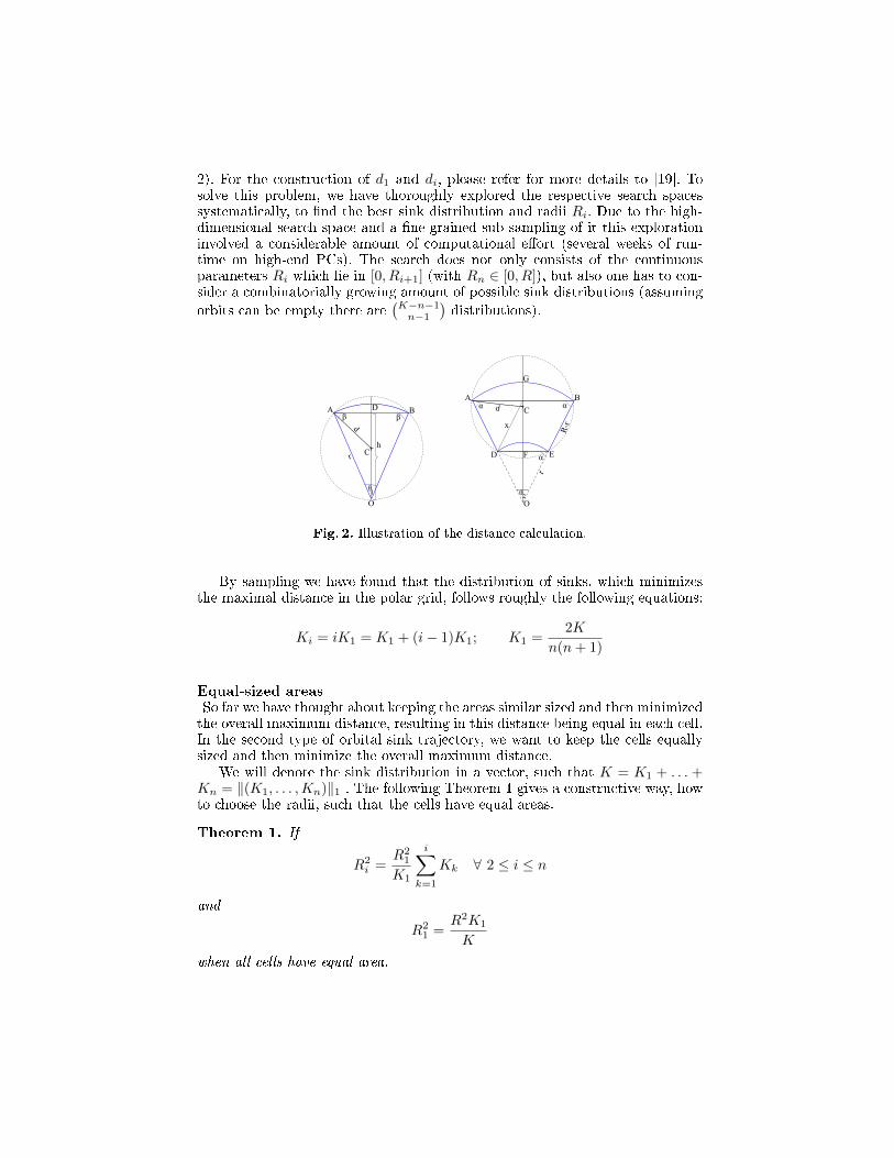
2). For the construction of d1 and di, please refer for more details to [19]. Tosolve this problem, we have thoroughly explored the respective search spacessystematically, to �nd the best sink distribution and radii Ri. Due to the high-dimensional search space and a �ne-grained sub-sampling of it this explorationinvolved a considerable amount of computational e�ort (several weeks of run-time on high-end PCs). The search does not only consists of the continuousparameters Ri which lie in [0, Ri+1] (with Rn ∈ [0, R]), but also one has to con-sider a combinatorially growing amount of possible sink distributions (assuming

orbits can be empty there are(K−n−1n−1

)distributions).

Fig. 2. Illustration of the distance calculation.

By sampling we have found that the distribution of sinks, which minimizesthe maximal distance in the polar grid, follows roughly the following equations:

Ki = iK1 = K1 + (i− 1)K1; K1 =2K

n(n+ 1)

Equal-sized areasSo far we have thought about keeping the areas similar sized and then minimizedthe overall maximum distance, resulting in this distance being equal in each cell.In the second type of orbital sink trajectory, we want to keep the cells equallysized and then minimize the overall maximum distance.

We will denote the sink distribution in a vector, such that K = K1 + . . . +Kn = ‖(K1, . . . ,Kn)‖1 . The following Theorem 1 gives a constructive way, howto choose the radii, such that the cells have equal areas.

Theorem 1. If

R2i =

R21

K1

i∑k=1

Kk ∀ 2 ≤ i ≤ n

and

R21 =

R2K1

K

when all cells have equal area.

Proof. Let 2 ≤ i ≤ n be arbitrary, when the area of a cell in the k -th orbit isgiven by:

Ai =π(R2

i −R2i−1)

Ki=πK−11 R2

1(∑ik=1Kk −

∑i−1k=1Kk)

Ki

=πR2

1

K1= A1

Where A1 is the area of a cell of the �rst orbit. Further one sees easily thatRn = R .

Under the same polar grid area assignment, the maximum distances for thetriangle d1 and for the trapezoid di can be computed according to the Equation1 and 2.

However, it is still unclear how to distribute the sinks optimally, such that alow maximal Euclidean distance is achieved. So we still have to deal with thecombinatorial explosion of possible sink distributions. Also for this approachwe decided to search systematically for the best solution. Having a closed formof radii distribution under the equal-sized area, sampling can be done muchfaster. Based on the results by sampling, the sinks distribution Ki can be derivedroughly as the following:

Ki = K1 + 2(i− 1)K1; K1 =K

n2

Table 2. Comparison of MD and EA Methods.

Minimum Euclidean Distance Equal Sized Area

Sink

distribution

K1Ki

= 1i

K1Ki

= 12i−1

Orbits' radii Ri = i · Rn Ri = i · RnRelationship

of K, K1,and

n

K = K1

n∑i=1

i K = K1

n∑i=1

2i− 1

Comparing the two strategiesThe results of these computations for four orbits (for other numbers of orbitsthe results look similar) can be found in Figure 3. One can observe in the �rst�gure that the radii converge to Ri = i · Rn . As seen in Figure 3 the di�erencebetween the two approaches lies mainly in the sink distribution. They follow therules presented in Table 2, the dashed lines in the �gures represent how the sinkdistribution, for 100 sinks, would have to look like, if one applies the rule.

Both strategies have in common that the radii are converging to the samevalues Ri = iRn , which can be seen esspecailly for low n . Also they share thelinear increasement of sinks in the orbtis, but with di�erent rates. One could see

Four Orbits’ Radii Distribution (MD vs. EA)

#sinks

Euclid

ean d

ista

nce (

m)

12 18 24 30 36 42 48 54 60 66 72 78 84 90 96

0

25

50

75

100 MD

EA

12 18 24 30 36 42 48 54 60 66 72 78 84 90 96

Four Orbits’ Sink Distribution (EA)

#sinks

sin

k d

istr

ibution

0

20

40

60

80

100

K1

K

KK

2

3

4

K1

K1+3K

1

+5K1

K1+3K

1

+7K1

+5K1

K1+3K

1

12 18 24 30 36 42 48 54 60 66 72 78 84 90 96

Four Orbits’ Sink Distribution (MD)

#sinks

sin

k d

istr

ibution

0

20

40

60

80

100

K1

K1+2K

1

+3K1

K1+2K

1

+4K1

+3K1

K1+2K

1

K1

K

KK

2

3

4

Fig. 3. Radii and Sink distributions for MD and EA.

the two strategies as special cases of an more general approach which distributesthe sinks in the following way:

Ki = K1 + γ(i− 1)K1; K1 =2K

n(nγ − γ + 2)(1)

For γ = 1 this results in the approach of minimizing the maximal distance(further called MD) and for γ = 2 we get the equally sized area approach (furthercalled EA). (For γ = 0 one gets an euqal distribution of sinks over the orbits.)There are other values for γ imaginable, resulting in hybrid approaches, however,we will not consider other values for γ in this report. For the rest of the reportwe set Ri = i · Rn to make further steps tractable.

We hope to see that equally sized cells are performing better in terms ofenergy and the strategy which concentrates on minimizing the maximal distanceis doing better in terms of delay. Further for values of γ between 1 and 2 wehope to see how the tradeo� between energy and delay developes.

4.3 Choosing the Right Number of Orbits

Clearly, choosing the right number of orbits is an important factor. In the smallerscale setting of our previous work [19] we found signi�cant gains when going from

a single orbit to a two-orbit trajectory. Hence, in the very large-scale WSNsthat we target in this work, we have to �nd out which number of orbits isoptimal. For this purpose, we compute for di�erent number of sinks the optimalnumber of orbits by checking through all numbers of orbits from 1 up to 100for both, MD and EA. How this computation was performed for a given numberof sinks is shown in Algorithm 1. The algorithm takes as inputs, the number ofsinks and the value of γ and outputs the number of orbits, which results in thesmallest maximal Euclidean distance between any point and its allocated sink.The alert reader may notice that the algorithm takes only the �rst and last orbitinto account for calculating the maximal Euclidean distance. This is due to thefollowing lemma:

Lemma 1. Let K and n be such that 3n(nγ−γ+2) ≤ 2K, then di is increasingin i for all i ≥ 2.

Proof. Let K sinks be given and let n ≥ 1 such that 3(nγ−γ+2)n ≤ 2K . Thende�ne as before:

Ri = iR

n

For the sink distribution we have to think about, what happens, when the totalnumber of sinks is not such a multiple of K1 that (1) is full�lled. We start byde�ning

K1 =

⌊2K

n(γn− γ + 2)

⌋and Ki = bK1 + γ(i− 1)K1c

and denote the rest of the sinks by L :

L = K −n∑i=1

Ki

Lemma 2. The chosen distribution ful�lls:∑i

Ki = K

Proof. ∑i

Ki =∑i

iK1 + li = L+∑i

iK1 = K

.

Lemma 3. It holds K1 ≥ 3

Proof. Since 3(γn− γ + 2)n ≤ 2K we have 2Kn(γn−γ+2) ≥ 3 , from which follows

b 2Kn(γn−γ+2)c ≥ 3 .

For calculating the maximal distance d(n) in the polar grid, we would needto calculate the distances in the orbits di(n) . To calculate these distances weneed to know, if we are considering "short" trapezoids or "long" trapezoids. Thefollowing theorem shows, that we have to consider only "short" trapezoids in allorbits, which makes the upfollowing calculations much easier.

Theorem 2. For all orbits holds that the resulting trapezoids are short, i.e.

| AB |2≤ x (3)

Proof. Fix some i and assume �rst that L = 0 , then

| AB |2

= iR

nsin(

π

(γi− γ + 1)K1)

and

x2 = R2i sin

2(π

(γi− γ + 1)K1)− 2RiRi−1 sin

2(π

(γi− γ + 1)K1) +R2

i−1

Hence (3) is equivalent to the condition that:

2RiRi−1 sin2(

π

(γi− γ + 1)K1) ≤ R2

i−1

Which is, by inserting values for the radii, equivalent to the condition:

i− 1 ≥ 2i sin2(π

(γi− γ + 1)K1)

1 ≤ i(1− 2 sin2(π

(γi− γ + 1)K1) = i cos(

2π

(γi− γ + 1)K1)

This is ful�lled for all i ≥ 2 and all K1 ≥ 3 , γ ∈ [1, 2] .To give the maximal distance in the whole polar grid, it su�ces to calculate

the maximal distance in the n -th orbit, if L = 0 :

Theorem 3. di(n) is an increasing function in i ≥ 2 for all γ ∈ [1, 2] .

Proof. We know that:

di(n) =R(1 + 4(i− 1)i cos2(π2 −

π(γi−γ+1)K1

))12

2n sin(π2 −π

(γi−γ+1)K1)

=R

n(

1

4 sin2(π2 −π

(γi−γ+1)K1)+ (i− 1)i cot2(

π

2− π

(γi− γ + 1)K1))

12

Since di(n) is positive, it is su�cient to show that (di(n))2 has positive derivative,

which is given by:

Di(d2i (n)) =

− cos(π2 −π

(γi−γ+1)K1) sin(π2 −

π(γi−γ+1)K1

)( γπ(γi−γ+1)2K1

)

2 sin4(π2 −π

(γi−γ+1)K1)

+(4i− 2) cos2(π2 −

π(γi−γ+1)K1

) sin2(π2 −π

(γi−γ+1)K1)

2 sin4(π2 −π

(γi−γ+1)K1)

−4(i2 − i) cos(π2 −

π(γi−γ+1)K1

) sin2(π2 −π

(γi−γ+1)K1)( γπ

(γi−γ+1)2K1)

2 sin4(π2 −π

(γi−γ+1)K1)

Since the denominator is larger zero for all i ≥ 2 , K1 ≥ 3 and γ ∈ [1, 2] we canconcentrate on the numerator. Note that we can factor out:

cos(π

2− π

(γi− γ + 1)K1) sin(

π

2− π

(γi− γ + 1)K1) =

1

2sin(π− 2π

(γi− γ + 1)K1) ≥ 0

Hence we have to prove:

(2i−1) sin(π− 2π

(γi− γ + 1)K1) ≥ γπ

(γi− γ + 1)2K1(4(i2−i) sin(π

2− π

(γi− γ + 1)K1)+1)

(4)We start with the left side of (4). Using Taylor-Expansion around π we have:

(2i−1) sin(π− 2π

(γi− γ + 1)K1) ≥ (2i−1)

(2π

(γi− γ + 1)K1− (

2π

(γi− γ + 1)K1)4

1

4!

)the right side of (4) will be also treated by a Taylor-Expansion around π ::

γπ

(γi− γ + 1)2K1(4(i2 − i) sin(π

2− π

(γi− γ + 1)K1) + 1)

≤ γπ

(γi− γ + 1)2K1(4(i2 − i)( π

(γi− γ + 1)K1+

π3

3!(γi− γ + 1)3K31

) + 1)

Comparing these two expressions we need to show:

(2i− 1)(2(γi− γ + 1)− π3

3(γi− γ + 1)2K31

)

≥4γ(i2 − i)( π

(γi− γ + 1)K1+

π3

3!(γi− γ + 1)3K31

) + γ

Next we will eliminate the parameter γ by noting that γ ∈ [1, 2] and hence(γi− γ+1) ∈ [i, 2i− 1] . The expressions (3) and (4) can hence be bounded andwe can simplify the inequality further:

(2i− 1)(2i− π3

3i2K31

≥ 8(i2 − i)( π

iK1+

π3

3!i3K31

) + 2

Multiplying this by 3i2K31 the inequality can be rewritten into a multinomial in

K1 and i :

12i4K31 − i3(6K3

1 + 24πK21 ) + i2(24πK2

16K31 )− 6iπ3 + 5π3 ≥ 0

With standard methods of analysis one can show, that this inequality is ful�lledfor each K1 ≥ 3 and i ≥ 2 (see also the next part). Hence (4) is ful�lled for allγ ∈ [1, 2] and by this the derivative Di(d

2i (n)) is positive.

Then, di can be given by:

di =R

n

( 1

4 sin2(π2 −π

(γi−γ+1)K1)+

(i− 1)i cot2(π

2-

π

(γi− γ + 1)K1))1/2

.

Algorithm 1 Computing the optimal number of orbits.

Inputs: The number of sinks K, the network radius R, and

the parameter γ =

{1 for MD

2 for EA.

for n = 1 to 100 do1. Compute K1 = 2K

n(γn−γ+2)

2. if (K1 ≥ 3)

2.1. Compute d1 =

{R

2n sin(π2− πK1

)for K1 > 3

Rncos(π

2− π

K1) for K1 = 3

2.2. Compute

dn = Rn

12 sin(π

2− πγn−γ+2

)

√1 + 4(n− 1)n cos2(π

2− π

γn−γ+2)

2.3. Compute Dnmax = max{d1, dn}

endforreturn orbit j such that Dj

max = min1≤i≤nDimax

Since di is positive, it is su�cient to show that d2i has a positive derivative, afterfactoring outcos(π2 −

π(γi−γ+1)K1

) sin(π2 −π

(γi−γ+1)K1) ≥ 0, its numerator (the denominator is

positive) can be given by

(2i− 1) sin(π − 2π

(γi−γ+1)K1

)− πγ

(γi−γ+1)2K1

(4(i2 − i) sin(π2 −

π(γi−γ+1)K1

) + 1).

using a Taylor-Expansion around π for the �rst sum and using that sin(x) ≤ 1for all x, we know that the above expression is larger than zero, if

2π3

3i2K31

≤ 1

which is true for all i ≥ 2 and K1 ≥ 3, which is the case by our assumptions onK and n.

The condition of the lemma is not restrictive, as, for sink distributions ac-cording to Table 2, it translates to having at least three sinks per orbit. Havingtwo or less sinks in one orbit would mean to place them in the center of thewhole sensor �eld as this minmizes the Euclidean distance, e�ectively wasting acomplete orbit. Hence, excluding such cases does not in�uence the best selectionof orbits. The optimal number of orbits for di�erent number of sinks (up to 200)and the di�erent approaches are displayed in Table 3.

4.4 Distribution of Leftover Sinks

In our rules for the sink distribution we handle the sinks as real numbers. Ofcourse, they are integral and thus we simply use the following sink distribution:

K1 =⌊

2Kn(γn−γ+2)

⌋; Ki = bK1 + γ(i− 1)K1c

Table 3. The optimal number of orbits for MD and EA.

MD(#sinks) EA(#sinks) #orbits

3-8 3-11 1

9-18 12-29 2

19-35 30-59 3

36-59 60-98 4

60-90 99-146 5

91-127 147-200 6

128-170 - 7

171-200 - 8

Algorithm 2 Handling of leftover nodes for MD and EA.

Inputs: The number of sinks K, the number of orbit n, the network radius R and the

parameter γ =

{1 for MD

2 for EA.

Begin:

1. Compute K1 =⌊

2Kn(γn−γ+2)

⌋and

Ki = bK1 + γ(i− 1)K1c for i = 2n to 1002. Compute the leftover nodes L = K −

∑ni=1Ki

3. while(L 6= 0) do3.1. if (γ = 1) do

3.1.1. Find orbit j such that dj = max1≤i≤n di3.1.2. Kj++ and L- -end if

3.2. if (γ = 2) do3.2.1. Find orbit j such that aj = max1≤i≤n ai3.2.2. Kj++ and L- -end if

end while loopreturn Ki where i = 1, . . . , n such that K =

∑ni=1Ki

To run the experiments we choose di�erent distributions of the sinks by theabove formula for di�ering γ . However the fraction 2K

n(nγ−γ+2) is not an integer

for every n . In this cases we consider b 2Kn′(n′γ−γ+2)c and get an distribution which

consists of K ′ < K sinks. The remaining K −K ′ have to be distributed in somefashion which approximates the real values of Ki . Let L = K −

∑ni=1Ki 6=

0 is the number of leftover sinks. We deal with this leftover sinks simply bydistributing them over the orbits, in a greedy fashion, according to the goal ofthe respective approach. In the MD case, we place one sink at a time in theorbit which currently exhibits the maximal Euclidean distance, whereas in theEA case we place the sink in the orbit which contains the cells with the largestarea. Algorithm 2 illustrates this procedure.

5 Performance Evaluation

In discrete-event simulations, we evaluate the delay and the lifetime performanceof our heuristic framework by comparing it to three di�erent mobile sink trajec-tories and two static sink placement strategies.

5.1 Delay Performance

With the help of sensor network calculus (SNC) [20], we evaluate the worst-casedelay performance. To apply the SNC, the network tra�c has to be described interms of arrival curves αi for each node. An arrival curve de�nes an upper boundfor the input tra�c of a node. To calculate the outputs of the nodes service curvesβi are used. The service curve speci�es the worst-case forwarding capabilitiesof a node. Based on arrival and service curves, we use the Pay MultiplexingOnly Once (PMOO) analysis described in [22] for the end-to-end delay boundcomputation. A tool called DISCO Network Calculator [21] provides us with anautomated way of doing so.

5.2 Lifetime Performance

We de�ne the lifetime as the number of epochs until the �rst sensor node depletesits battery. The energy consumption for transmitting and receiving are takeninto account using an energy model based on MICAz motes [1]. The modelcomputes the energy level Env of each sensor node v in epoch n using the followingequations:

Env =∑w∈T nv

Etx(w, fn(w)) +∑w∈Rnv

Ercv(w, fn(w)), (5)

with

Ercv(w, fn(w)) =Ercv(fn(w)) = Prcv · trcv(fn(w)), (6)

Etx(w, fn(w)) =Ptx(w) · ttx(fn(w)). (7)

Here, T nv and Rnv denote the set of nodes to send to and receive from for v inepoch n. In (6), we see that the energy consumption for receiving fn(w), theamount of data from node w in epoch n, is just the time needed to receive thedata trcv(fn(w)) multiplied by the power consumption Prcv of the receiving unit;this is independent of the distance between the sending and receiving node. In(7), the energy consumption for sending data is again the time needed to sendthe data ttx(fn(w)) times the power consumption of the sending unit Ptx(w),which, however, now is dependent on the distance to w. Taking the values fromthe MICAz data sheet [1], we can calculate the power consumed by the receiverelectronics Prcv and the transmitting electronics Ptx(w). The exact dependenciesof Ptx(w) on the distance to w is described by a model for the MICAz mote,which can be found in [25].

5.3 Competitors

We have realized di�erent competitors to compare our heuristic with. Unfortu-nately, the �eld of multiple mobile sink for very large WSNs is barely tappedso it was hard to �nd direct competitors. To create competitors we generalizedideas from other (smaller scale) proposals ([12], [7], [16]). The competitors arebrie�y described in the following; some of them are illustrated in Figure 4.

Random Walk: Initially, sinks are placed uniformly randomly in the sensor�eld. At the start of each epoch, the sinks randomly choose a direction and stepsize (ensuring, however, that they do not leave the sensor �eld). We use thiscompetitor as a baseline and also because it has been discussed in literature [4].

Outer Periphery: [12] remarks that, in the single sink case, a trajectory alongthe periphery of the network optimizes the lifetime by balancing the load dis-tribution. We generalize this concept by moving each of our sinks along the cellperipheries, where the cells are formed according to the MD approach.

Following the Energy (FE): In this strategy, the sinks are placed randomlyover the network area for the �rst epoch. For the following epochs, the K sensornodes with the highest residual energy left are identi�ed and the sinks movenear to them. We use this one only as a competitor for lifetime, as its delaypeformance is very bad. It represents the group of state-aware trajectories (e.g.[16]).

K-Center Heuristic: [7] presents a polynomial 2-approximation for the NP-hard K-center optimization problem. The competitiveness of the algorithm isillustrated by the result of [8] which shows that if there exists an δ-approximationwith δ < 2 this results in NP = P . The authors use their algorithm on afully connected weighted graph, nevertheless the idea can be carried over toour graph (see Appendix I). This is a competitor only for the worst-case delay,as it performs badly with respect to lifetime due to being static. It serves asa representative for algorithms based on graph-theoretic abstractions and wasexpected to perform very well for delay due to its nice theoretical properties.

Static MD: This takes the same sink distribution as generated by our MDheuristic, but the sinks are not moving. Instead we run the MD strategy for awhole set of possible positions and choose the one, which has minimal delay. Thisobviously bad lifetime competitor is included to show both, how the lifetime ofthe network is increased by mobility as well as its negative e�ect on delay.

5.4 Experimental Set Up

Using discrete-event simulations, we evaluate the worst-case delay and the life-time performance of our heuristic framework. In the experiments, nodes areuniformly distributed over a circular �eld with radius R. The respective network

O

R

RR

(a) (b) (c)

Fig. 4. Competitors: (a) a random walk, (b) an outer periphery trajectory, and (c) astatic MD.

radii are chosen such that always a node density of 1100m2 is achieved. A 20m

disc-based transmission range is used under a shortest path routing for the sinktrees. Token-bucket arrival curves and rate-latency service curves are consideredfor SNC operations. In particular, for the service curve we use a rate-latencyfunction that corresponds to a duty cycle of 1% and it takes 5ms time on dutywith a 500ms cycle length which results in a latency of 0.495 s1. The correspond-ing forwarding rate becomes 2500 bps. Initially, the nodes are set to an initialbattery level of 0.1 joule. Packets of 100 bytes length are sent to the correspond-ing sinks. Apart from static sinks, all others move synchronously to their nextposition between epochs. The MD and EA methods use a movement angle ofθ = 10°. To compute the energy consumption (Equation 5), we use the follow-ing data based on [25, 1]. The current consumption is 8.5mA with−25 dBm fordistances up to 12.5m, and 9.9mA for distances between 12.5m and 23m with−20 dBm. For receiving a data packet, a 1% duty cycle is considered with acurrent of 19.7mA. A constant voltage of 3V is used. A transmission data rateof 250Kbps is used, which takes ttx = 3.2ms for a 100 byte packet.

5.5 Results

We analyze the following three scenarios: 1500 nodes with 15 sinks, 5000 nodeswith 50 sinks, and 10000 nodes with 100 sinks. So, we keep a constant node tosink ratio of 100 nodes/sink. For each scenario, we analyze the energy consump-tion per epoch, the lifetime and the worst-case delay. For all experiments, weperformed 10 replications and present the average results from these. For thelarge majority of results, we obtained non-overlapping 95% con�dence intervals,so we do not show these in most of the graphs for reasons of legibility. The staticMD and the K-center heuristic are static sink placements so that we computethe lifetime based on the overall number of packets transmitted and translate itinto an equivalent number of epochs (using the results from the other methods).

Worst-Case Delay Evaluation Figure 5 compares the delay performanceof the four mobile sinks and two static sinks strategies. In all scenarios, the

1 The values are calculated based on the TinyOS �les CC2420AckLpl.h andCC2420AckLplP.nc.

dela

y b

ou

nd (

s)

competitors

05

10

15

20

25

30

Random Walk (RW)

Outer Periphery (OP)

EA

MD

Static MD

K−Center

RW OP EA MD Static MD K-Center

dela

y b

ou

nd (

s)

competitors

05

10

15

20

25

30

Random Walk (RW)Outer Periphery (OP)EAMDStatic MDK−Center

OPRW EA MD Static MD K-Center

dela

y b

oun

d (

s)

competitors

05

10

15

20

25

30

Random Walk (RW)Outer Periphery (OP)EAMDStatic MDK−Center

RW OP EA MD Static MD K-Center

05

10

15

lifetime (in number of epochs)

tota

l e

ne

rgy c

onsum

ptio

n (

%)

1 2 3 4 5 6 7 8 9 10 11

Outer Periphery (OP)

Following the Energy (FE)

Random Walk (RW)

MD

EA

Static MD

OP

FE

RW

MDEA

Static MD

05

10

15

lifetime (in number of epochs)

tota

l e

ne

rgy c

on

sum

ptio

n (

%)

1 2 3 4 5 6 7 8 9 10 11

Outer Periphery (OP)

Following the Energy (FE)

Random Walk (RW)

MD

EA

Static MD

OP

FE

RW

MD

EA

Static MD

05

10

15

lifetime (in number of epochs)

tota

l e

ne

rgy c

onsum

ptio

n (

%)

1 2 3 4 5 6 7 8 9 10

Outer Periphery (OP)

Following the Energy (FE)

Random Walk (RW)

MD

EA

Static MD

OP

FE

RW

MD

EA

Static MD

(a) (b) (c)

Fig. 5. Delay and lifetime performance comparison: (a) 1500 nodes and 15 sinks, (b)5000 nodes and 50 sinks, and (c) 10000 nodes and 100 sinks.

best delay performance is achieved by the static MD, closely followed by ourmobile sinks strategies EA and MD. As already discussed in Section 1, thereis a price to pay for the prolonged lifetime by mobile sinks in terms of delay,yet as we see here that price is rather low. EA and MD perform almost equallywell with a slight advantage for EA. More importantly, both of them achieveroughly the same delay performance across the di�erent scenarios and are thusscalable with respect to delay. For the outer periphery and the random walk, theassessment is very di�erent: their delay performance is much worse and also thedelay increases with growing network size, so they do not scale well with respectto delay. Somewhat surprisingly, the K-center heuristic, which requires a highcomputational e�ort and centralized information, is not doing particularly welland is actually slightly outperformed by the mobile trajectories EA and MD,which indicates again that their delay performance is very good.

Lifetime Evaluation The simulation results for the lifetime performance ofthe competitors are shown in Figure 5. The graph shows the total energy con-sumption in the sensor �eld over the number of epochs, so the lengths of thelines indicates the lifetime performance of the respective method. Looking overall scenarios, MD turns out to be the clear winner with respect to lifetime. EAbasically achieves the same lifetime in the 1500-nodes scenario, but cannot keepup with MD in the larger scenarios. All other competitors perform rather poorly:the random walk is a complete failure with a lifetime of 1.5 epochs in the largestscenario; the FE strategy also performs very bad and does not ful�l the hopesone could have in a state-aware trajectory (admittedly it is a simple strategyand more sophisticated state-aware trajectories could be doing better); the outerperiphery strategy is a little bit better, but at the expense of a high overall en-ergy consumption. Interestingly, the static MD does not perform too badly, itoutperforms FE and the random walk, which shows that trajectory planning

0 5 10 15 20 25 30

02

46

810

12

Life

tim

e (

in n

um

be

r o

f e

po

ch

s)

Delay bound (s)

MD

EA

Static MD

Outer Periphery

Random Walk

Fig. 6. Lifetime-delay tradeo� among competitors.

must be done with care otherwise one could do even worse than a good staticstrategy. On the other hand, we can see very clearly the lifetime prolongatione�ect of using mobile sinks when comparing static MD with the MD sink trajec-tory: for example, in the 1500-nodes scenario MD achieves 10.8 epochs whereasstatic MD achieves only 4.6 epochs.

Lifetime vs. Delay and Scalability In this subsection, we somewhat wrapup the previous results by particularly looking at the combined lifetime vs. delayperformance as presented in Figure 6. The x-axis represents the delay and they-axis shows the corresponding lifetime performance in terms of the number ofepochs. The shape and color of the symbols represents the di�erent strategiesand the size of the symbols encodes the scale of the experiment, i.e., the largesymbols represent the experiments with 100 sinks, while the medium-sized andsmall symbols represent the experiments with 50 and 15 sinks, respectively. Byfollowing the path from small to large symbols one can see, how the strategiesscale for larger WSNs. Clearly, the goal must be to stay within the upper leftquadrant of this graph. Only MD achieves this goal, EA has a problem withrespect to lifteime scalability. All other competitors do not really o�er goodlifetime-delay tradeo�s and are at best good in one of them.

One may even become suspicious about MD for its scalability, because as canbe observed in Figure 6, there is a certain degradation with respect to lifetimefor it, too. However, the lifetime de�nition that we use here (when the �rstnode dies) somewhat looses its usefulness with an increasing number of nodes,as it becomes more and more likely that some single node is in an unfortunateposition where its battery is drained much quicker than for others. Therefore,we provide some more information on the �death� process of the nodes in the�eld when we continue network operation after the �rst node died in Figure 7(again the size of the symbols represents the scale of the scenario). In particular,when we rede�ne lifetime as the time until which 10% of the nodes have diedthen we see that MD scales very well, i.e., it achieves almost the same lifetimein all three scenarios. In comparison, EA still does not scale that well, thougharguably it also bene�ts from this rede�nition of the lifetime.

0 5 10 15 20 25 30

02

00

40

06

00

80

01

00

0

lifetime (in number of epochs)

#d

ea

d n

od

es

MDEA

Fig. 7. MD/EA lifetime performance under a di�erent de�nition.

6 Conclusion and Outlook

In this report, we have proposed a �exible heuristic framework to design thetrajectories for multiple mobile sinks such that a good tradeo� between a highnetwork lifetime and a low information transfer delay can be achieved in verylarge sensor networks. The framework uses an n-orbit model which is based ona geometric rationale that, in large sensor networks, cell areas and Euclideandistances between nodes and sinks are good proxy measures for lifetime anddelay. Two instances of the framework are derived: one which focuses on theminimization of the maximal Euclidean distances (MD), and one which targetsto equalize the area assignment and takes distance minimization as a secondarygoal (EA). Both are compared with several competitors in detailed discrete-eventsimulations and show very good lifetime-delay tradeo�s. Especially, the MDstrategy shows a very scalable behavior for its lifetime and delay performancewhen the number of nodes becomes large. In particular, in contrast to all othermethods it keeps up the delay and lifetime values of smaller scenarios whenscaled to larger scenarios under a constant node-to sink ratio. More abstractly, webelieve to have provided strong evidence that the orbital sink trajectories providefor a natural scalability to very large sensor networks, if designed carefully.

To conclude the report, we want to discuss some relaxations of the assump-tions in our framework and how the geometric interpretation can still be helpful,thereby pointing out directions for future work: One assumption is the circu-lar shape of the sensor �eld. Smaller distortions (linear transformations) of thiswould result in ellipsoid shapes, which can still be dealt with a similarly distortedorbit model (mapping the position of the sinks by the same transformation tothe new sensor �eld). A change of the underlying distance norm would result incompletely di�erent shapes, we could think of a squared network area as a circleunder the maximum norm || · ||∞ (similarly one could change to the || · ||1-normto handle a rhombus-shaped sensor �eld). Another assumption is the uniform

distribution of nodes over the �eld. In some networks, there might be clustersof high density and regions with low density. Here more sinks are needed inthe clusters, while the sparse areas can be handled by less sinks, this could beachieved by altering the distances the sinks move between the epochs in ourorbit model. Slowing the sinks down, when reaching the clusters would result inaccumulating sinks in that region and speeding them up again, when leaving theclusters, moves them fast through the sparse areas.

Appendix I : The K-Center Heuristic

The K -Center heuristic of Hochbaum and Shmoys will be presented and modi-�ed, such that it �ts our needs. The K -Center heuristic is at its core a bisectionsearch other the optimal value for the paramter �mid�. The algorithm chooseswith the help of this parameter a set of sinks, if this set has less than K or justK elements, the parameter �mid� must be decreased (because we can assumeto achieve a better maximal distance, if we can place more sinks), if the set islarger than K we have to increase �mid�, since we are using too much sinks. Theoriginal algorithm works on a fully connected, edge-weighted graph, satisfyingthe triangle-inequality. Hochbaum and Shmoys algorithm is a 2-approximation,which is best possible, in the sense that �nding a δ -approximation wit polyno-mial runtime and δ < 2 leads to NP = P . Before we explain the algorithm, weneed some notations. We talk of G = (V,E) being a complete graph with edgeweights w the edges are sorted by their weight, this means:

w(ei) ≤ w(ej) ∀ i < j ≤ m = |E|

The graph is stored in adjacency-list-form. This means for each vertex v theadjacent vertices are listed in increasing edge weight order. We need two morenotations Gi = (V,Ei) , where Ei = {e1, . . . , ei} and ADJi(x) which is theadjacency list of x in Gi . Next we will present the Algorithm 3 as it can befound in the paper of Hochbaum and Shmoys:

To adapt this algorithm to our report we made a few changes. At �rst oursensor network is not fully connected and on the other side links have no weights.we solve these two problems by using the euclidean distances between the nodesas link weight and assume the network to be fully connected. Further we are notoperating an a complete list of edges, instead each node has its own list, whichagain contains the neighbours of the node in the order of increasing edge-weights.for this we denote by n(v) = (xv,1, xv,2, . . . , xv,N ) the vector of neighbours of vand by ni(v) = (xv,1, xv,2, . . . , xv,i) the �rst i neighbours of v . Watch out thatni(v) 6= ADJi(v) , in the �rst vector we have pruned the list of v to i neighbours.In the second vector we have pruned the complete set of edges to Ei and thentake all neighbours of v which are left. A second change to the original algorithmis, that we are not deleting the neighbours of the neighbours of v from the set T .Instead we are just deleting the neighbours of v , which leads to less coordinationbetween the nodes. The Algorithm 4 looks then like this:

Algorithm 3 The K-Center Heuristic.Begin:low:= 1;high:= m;if k =| V |S = V ;endwhile high > low + 1 do

mid:= bhigh+ low2 c

S := ∅;T := V ;while ∃x ∈ T doS := S ∪ {x};for v ∈ ADJmid(x) doT := T − ADJmid(v)− {v};

endendif | S |6 khigh := mid;S′ := S;endif | S |> klow := mid;end

end

end

Algorithm 4 The K-Center Heuristic for WSN.Begin:low:= 1;high:= N ;if k =| V |S = V ;endwhile high > low + 1 do

mid:= bhigh+ low2 c

S := ∅;T := V ;while ∃x ∈ T doS := S ∪ {x};T := T − nmid(x); First we have to convert the vector to a set at this line.

The set is built simply by collecting all entries of the vector.endif | S |6 khigh := mid;S′ := S;endif | S |> klow := mid;end

end

end

If the algorithm outputs a set of sinks which has less than K elements, weplace the di�erence of sinks randomly over the network. Note that as a resultof this sink placement, we can bound the maximal euclidean distance from anynode to the nearest sink by:

maxv∈V{xv,mid}

Bibliography

[1] Crossbow technology inc. mpr-mib users manual, June 2007.[2] S. Basagni, A. Carosi, E. Melachrinoudis, C. Petrioli, and Z. M. Wang.

Controlled sink mobility for prolonging wireless sensor networks lifetime.Wireless Sensor Network, 14(6):831�858, December 2008.

[3] S. Basagni, A. Carosi, and C. Petrioli. Heuristics for lifetime maximizationin wireless sensor networks with multiple mobile sinks. In Proc. IEEE ICC,June 2009.

[4] I. Chatzigiannakis, A. Kinalis, S. Nikoletseas, and J. Rolim. Fast and energye�cient sensor data collection by multiple mobile sinks. In Proc. 5th ACMInt. Workshop. on Mobility Management and Wireless Access, pages 25�32,2007.

[5] C. Chen, J. Ma, and K. Yu. Designing Energy-E�cient Wireless SensorNetworks with Mobile Sinks. In Proc. ACM SenSys, October 2006.

[6] S. Gao, H. Zhang, and S. Das. E�cient Data Collection in Wireless SensorNetworks With Path-constrained Mobile Sinks. In Proc. IEEE WoWMoM,October 2009.

[7] Dorit S. Hochbaum and David B. Shmoys. A best possible heuristic forthe k-center problem. Mathematics of Operations Research, 10(3):180�184,May 1985.

[8] Wen-Lian Hsu and George L. Nemhauser. Easy and hard bottleneck locationproblems. Discrete Applied Mathematics, 1:209�215, 1979.

[9] W. Liang, J. Luo, and X. Xu. Prolonging network lifetime via a controlledmobile sink in wireless sensor networks. In Proc. IEEE Globecom, 2010.

[10] Y. Liu, G. Zhou, J. Zhao, G. Dai, X.Y. Li, M. Gu, H. Ma, L. Mo, Y. He,J. Wang, M. Li, K. Liu, W. Dong, and W. Xi. Long-term large-scale sensingin the forest: recent advances and future directions of greenorbs. Frontiersof Computer Science in China, 4, 2010.

[11] J. Luo. Mobility in Wireless Networks: Friend or Foe - Network Design andControl in the Age of Mobile Computing. PhD thesis, School of Computerand Communication Sciences, EPFL, Switzerland, 2006.

[12] J. Luo and J.-P. Hubaux. Joint Mobility and Routing for Lifetime Elon-gation in Wireless Sensor Networks. In Proc. IEEE INFOCOM, volume 3,pages 1735�1746, March 2005.

[13] J. Luo and L. Xiang. Prolong the lifetime of wireless sensor networksthrough mobility: A general optimization framework. In Theoretical As-pects of Distributed Computing in Sensor Networks, pages 553 �588, June2010.

[14] M. Ma and Y. Yang. Data gathering in wireless sensor networks with mobilecollectors. In Proc. IEEE IPDPS, April 2008.

[15] M. Marta and M. Cardei. Improved sensor network lifetime with multiplemobile sinks. Pervasive and Mobile Computing, pages 542�555, 2009.

[16] M. Mudigonda, T. Kanipakam, A. Dutko, M. Bathula, N. Sridhar,S. Seetharaman, and J.O. Hallstrom. A mobility management frameworkfor optimizing the trajectory of a mobile base-station. In Proc. EWSN,2011.

[17] I. Papadimitriou and L. Georgiadis. Maximum lifetime routing to mobilesink in wireless sensor networks. In Proc. SoftCOM, September 2005.

[18] W. Y. Poe, M. Beck, and J. B. Schmitt. Planning the Trajectories ofMultiple Mobile Sinks in Large-Scale, Time-Sensitive WSNs. Tech. Report381/11, University of Kaiserslautern, Germany, February 2011.

[19] W. Y. Poe, M. Beck, and J.B. Schmitt. Planning the Trajectories of MultipleMobile Sinks in Large-Scale, Time-Sensitive WSNs. In Proc. IEEE DCOSS,2011.

[20] J. B. Schmitt and U. Roedig. Sensor Network Calculus - A Framework forWorst Case Analysis. In Proc. DCOSS, June 2005.

[21] J. B. Schmitt and F. A. Zdarsky. The DISCO Network Calculator - AToolbox for Worst Case Analysis. In Proceeding of the First InternationalConference on Performance Evaluation Methodologies and Tools (VALUE-TOOLS'06). ACM, November 2006.

[22] J. B. Schmitt, F. A. Zdarsky, and L. Thiele. A Comprehensive Worst-Case Calculus for Wireless Sensor Networks with In-Network Processing. InIEEE Real-Time Systems Symposium (RTSS'07), pages 193�202, Tucson,AZ, USA, December 2007.

[23] R. C. Shah, S. Roy, S. Jain, and W. Brunette. Data MULEs: Modeling aThree-tier Architecture for Sparse Sensor Networks. In Proc. IEEE SNPA,pages 30�41, 2003.

[24] Y. Shi and Y. T. Hou. Theoretical Results on Base Station MovementProblem for Sensor Network. In Proc. IEEE INFOCOM, Phoenix, AZ,USA,2008.

[25] R. Shokri, P. Papadimitratos, M. Poturalski, and J. P. Hubaux. A Low-Cost Method to Thwart Relay Attacks in Wireless Sensor Networks. Proj.Report IC-71, 2007.

[26] A. A. Somasundara, A. Kansal, D. D. Jea, D. Estrin, and M. B. Srivastava.Controllably Mobile Infrastructure for Low Energy Embedded Networks.IEEE Transactions on Mobile Computing, 5:958�973, 2006.

[27] R. Sugihara and R. K. Gupta. Optimizing Energy-Latency Trade-o� inSensor Networks with Controlled Mobility. In Proc. IEEE INFOCOM,pages 2566�2570, Rio de Janeiro, Brazil, April 2009.

[28] S. Tang, J. Yuan, X.Y. Li, Y. Liu, G. H. Chen, M. Gu, J.Z. Zhao, andG. Dai. Dawn: Energy e�cient data aggregation in wsn with mobile sinks.In Proc. IWQoS, June 2010.

[29] Z. M. Wang, S. Basagni, E. Melachrinoudis, and C. Petrioli. Exploiting sinkmobility for maximizing sensor networks lifetime. In Proc. 38th Hawaii Int.Conf. on System Sciences, January 2005.

[30] Y. Yun and Y. Xia. Maximizing the lifetime of wireless sensor networks withmobile sink in delay-tolerant applications. In IEEE Trans Mobile Comput-ing, volume 9, pages 1308�1318, 2010.