ACCURATE SOIL WATER CONTENT MONITORING … · accurate soil water content monitoring in real time...

ACCURATE SOIL WATER CONTENT MONITORING IN REAL TIME WITH APPROPRIATE FIELD CALIBRATION OF THE FDR DEVICE “DIVINER 2000” IN A COMMERCIAL TABLE GRAPE VINEYARD

*J. Haberland1, R. Gálvez

2, C. Kremer

3, C. Zuñiga

4 and Y. Rudolffi

5

1Universidad de Chile, Facultad de Ciencias Agronómicas, 8820808, Av. Santa Rosa 11.315,

Santiago, Chile

E-mails: [email protected]

[email protected]

[email protected]

[email protected]

[email protected] (

*Corresponding Author)

Abstract: The purpose of this study was to determine the best field calibration method for

the FDR device “Diviner 2000”, and accurately monitor soil water content in real time in a

commercial table grape vineyard growing the Thompson Seedless variety. Field calibration

equations were obtained per depth (every 0.10m) and for the soil profile as a whole by

contrasting normalised probe readings with the actual volumetric water content (gravimetric

method) of three soil conditions i.e. dry, wet and saturated. The per-depth calibration was the

most precise, and was used to monitor water content in real time. One access tube was

located on the plant row, in three topographic locations: high (T1), middle (T2) and low (T3).

Field capacity (FC) and permanent wilting point (PWP) were determined for each tube. The

irrigation threshold chosen was a 30% depletion of available water (FC – PWP). Soil water

content went beyond the threshold (water deficit) 54.0% of the time in location T1 whereas it

went above FC (water excess) 46.8 % and 96.8% of the time in locations T2 and T3,

respectively. Being appropriately field calibrated, the Diviner 2000 proves effective in

accurately measuring soil water content in real time, which facilitates identification of

different irrigation management needs in the field.

Keywords: Capacitance probe, calibration, soil water content.

INTRODUCTION

The growing competition for water resources has made it necessary to improve water use

efficiency, especially in relation to irrigated agriculture, which consumes 87% of worldwide

water resources (FAO, 2003). In order to maximise productivity, “production per unit of

applied water” practices need to be adopted to reduce water losses (runoff, percolation and

evaporation) and avoid water stress during periods when the crop is most sensitive

(Intrigliolo et al., 2007). The evaluation and measuring of soil water content are critical

International Journal of Science, Environment ISSN 2278-3687 (O)

and Technology, Vol. 4, No 2, 2015, 273 – 284 2277-663X (P)

Received Feb 12, 2015 * Published April 2, 2015 * www.ijset.net

274 J. Haberland, R. Gálvez, C. Kremer, C. Zuñiga and Y. Rudolff

components of efficient irrigation management and help to establish better water preservation

practices (Muñoz-Carpena et al., 2004).

Soil water content affects plant growth and solute transportation in irrigated and non-irrigated

agricultural systems. Consequently, agricultural production is more closely related to the

available water in the soil than any other weather variable (DeJong and Bootsma, 1996) and

an extensive effort has been made to determine and characterise the variables controlling

water flow in the soil, and water absorption by the roots (Goldhamer et al., 1999).

Furthermore, localised and high-frequency irrigation systems modify root growth patterns as

well as water absorption by the plant, due to their particular water distribution pattern in the

soil (Bryla, 2004).

Girona et al. (2002) state that monitoring available water content in the soil is essential to

schedule irrigation due to the high variability of plant response, wetting patterns, soil depth

and root exploration in high-frequency irrigation systems. Among other factors, appropriate

irrigation scheduling requires soil water content measuring in real time.

The gravimetric method is the most precise method used to determine soil water content

(Gardner, 1986), however, it is disruptive and laborious, and does not allow the

measurement of water content in real time. Several non-invasive methods have been

developed, including neutron thermalisation (Greacen, 1981), tensiometers and electric

resistance sensors (Lowery et al., 1986; Spaans and Baker, 1992; Seyfried, 1993; Hanson et

al., 2000). Fairly recent technologies can measure soil water content continually, such as the

Time Domain Reflectometry (TDR) (Topp et al., 1980; Cassel et al., 1994) and electric

capacitance or Frequency Domain Reflectometry (FDR) (Robinson and Dean, 1993; Fares

and Polyakov, 2006).

The goal of this study was to obtain the best field calibration method for the FRD device

“Diviner 2000” to accurately monitor soil water content in real time in a commercial table

grape vineyard growing the Thompson Seedless variety.

MATERIALS AND METHODS

The field trial was carried out in a commercial table grape orchard growing the Thompson

Seedless variety (San José de Marchigüe, Region O´Higgins, Chile), with double-line drip

irrigation and emitters every 1m. The soil of the trial belongs to the coarse loam, mixed and

thermic family of the Vitradic Durixerolls (CIREN, 1996). Field observations were

performed in two soil phases.

Accurate Soil Water Content Monitoring in Real Time With ... 275

An FDR probe Diviner 2000 (Sentek Pty Ltd, Adelaide, SA) was normalised to obtain a

scaled frequency (SF) or normalised and then calibrated in the field. For the normalisation,

sensor frequencies in PVC tubes were observed when in contact with air (Fa) and in contact

with water at 22°C (Fw). The soil frequency (Fs) was used to obtain SF in Equation 1, which

in turn was used to obtain the volumetric soil water content (Өw) in Equation 2.

( ) / ( )SF Fa Fs Fa Fw= − − (1)

( / )B bSF A w w SF aθ θ= ⇔ = (2)

In order to obtain a complete range of soil water content, three soil water content conditions

were generated: dry (P1), wet (P2) and saturated (P3), 7m apart from each other. Condition

P1 was never irrigated, P2 was analysed with its current water content and P3 was flooded

until saturation and readings were done after a 48-h drainage period was allowed. Two access

tubes (PVC pipes, 0.5m length, 56.5mm interior diameter) were installed for each soil

condition, 6m apart (Figure 1), following manufacturer instructions. A double-ring rubber

plug was installed at the bottom of each tube to avoid water and/or vapour entering into the

access tube. The final arrangement of access tubes was 7x6m (Figure 1).

Three frequency readings were done every 0.1m in depth in each access tube. Immediately

after, two soil samples were taken from the soil profile using metallic cylinders, 0.30m from

each reading point. Samples were taken within the area of influence of the sensor (0.03m

from the access tube). Water content using the gravimetric method (W) and bulk density

(Db) using the cylinder method were obtained for each soil sample, and the volumetric

water content was estimated using Equation 3.

w WDbθ = (3)

A regression analysis was done between the values of volumetric water content and the

normalised frequencies provided by the device, in order to obtain calibration equations. The

regression analysis provided a determination coefficient. The standard error estimate (root-

mean-square error, RMSE) between the actual water content of the samples and the estimates

was determined for each calibration equation.

The soil water content was measuring on a real-time basis using the most precise equation(s)

obtained during the field calibration. One access tube was located on the plant row on three

topographic locations: high (T1), middle (T2) and low (T3) (Figure 2). Readings were done at

0.6m depths in locations T1 and T2, and 0.5m in location T3.


Soil phase 1 was observed in location T1 and soil phase 2 in locations T2 and T3. The water

retention curve was determined for both soil series, which provided field capacity (FC) and

permanent wilting point (PWP) values. The appropriate irrigation threshold reported for the

table grape is 30% of available water (AW = FC – PWP) depletion.

The field trial followed the farmer’s irrigation schedule. The criteria considered by the farmer

included general field observations and plant evapotranspiration measuring with data

collected from a local weather station and a crop coefficient from FAO. Table 1 shows the

soil water content (mm) at each topographic location at field capacity (FC), permanent

wilting point (PWP) and the irrigation threshold (at 30% AW depletion).

RESULTS AND DISCUSSION

Field calibration

Table 2 presents the results of the lineal regression determined by contrasting values of

volumetric water content obtained from the SF readings and the gravimetric method, for each

depth and soil profile as a whole (0 to 0.6m). The regression showed a high level of

adjustment to a power function, and coefficients a and b were obtained for Equation 2.

The field calibration per-depth equations showed a high correlation for the first 0.40 m of

depth (R2>0.91), whereas the correlation decreased (R

2 < 0.75) deeper in the soil profile. The

soil profile calibration equation showed an intermediate correlation (R2=0.81) regarding the

per-depth equations.

Several studies with FDR devices under laboratory conditions have found calibration

equations with higher determination coefficients for the soil profile than the one observed in

this study. Paltineanu and Starr (1997) obtained an R2 = 0.992 with the device

EnvironSCAN, and Groves and Rose (2004) obtained R2 ranging from 0.97 to 0.93 for

different soil profiles with a Diviner 2000. Da Silva et al., (2007) concluded that per-depth

calibrations show better correlation coefficients and minimise the RMSE value. On the other

hand, Morgan et al., (1999) found a calibration equation with R2 = 0.831 for the device

EnviroSCAN under field conditions, similar to the results reported by Haberland et al.,

(2014) (R2 = 0.98, in a clay and loam clay soils, RMSE 0.05 cm

3∙cm

-3) and in this study.

Bulk density is essential to determine volumetric soil water content, a basic element in the

calibration process. The determination of bulk density is among the main factors increasing

variability of soil water content measurements (Hu et al., 2008). It is expected to find more

precise results under laboratory conditions, where bulk density determination can be more


accurate and where newly developed methodologies, such as that described by Haberland et

al., 2014, ensure precise calibration.

Actual soil water content measured versus probe estimates

The probe provides water content values per depth, and for the soil profile by adding the

values obtained at different soil depths. The actual soil water content values were compared

to the values provided by the device with the different calibration options (Figure 3).

Figure 3 shows that both per-depth and profile field calibrations were more precise and

behaved more closely to the actual soil water content than the manufacturer calibration. The

calibration per depth showed the smallest variations in most of the cases.

Variations in the profile field calibration were always under 10%. In turn, per-depth field

calibration showed variations lower than 13%; similar results were found by Haberland et al.,

(2014), in which estimates presented a 13.76% error, and by Anderson et al., (2010),

underestimating by 9.1%.

Soil water content values under the manufacturer calibration were greater than 54% and

presented variations when using one or other calibration. However, the per-depth

measurement variations, from which the profile measurements come, were similar to the

calibration option. This incongruence is due to the overestimation of the actual soil water

content that the manufacturer calibration presents in almost every case. Therefore, per-depth

variations were additive, whereas in the field calibrations the measurements were

compensated. Several authors conclude that the field calibration of the Diviner 2000 is more

representative of the soil water content than the manufacturer calibration (Burgess et al.,

2006; Da Siva et al., 2007; and Haberland et al., 2014).

Soil water content monitoring

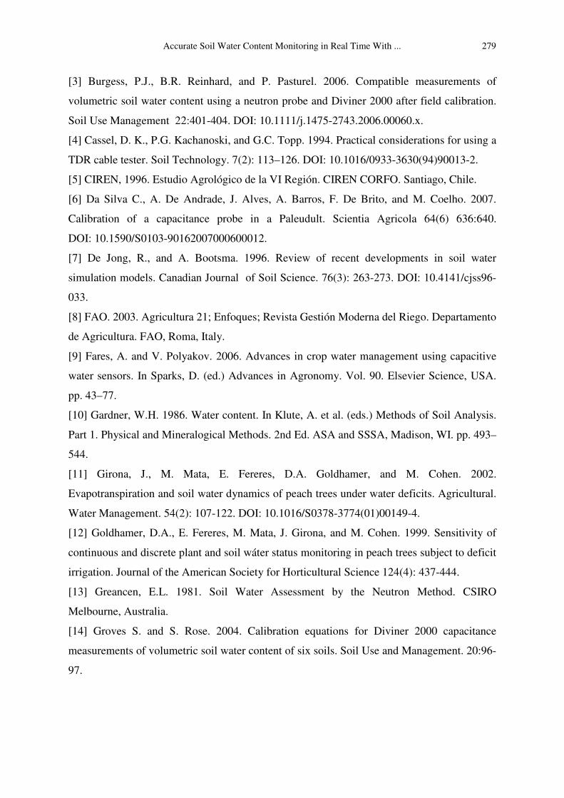
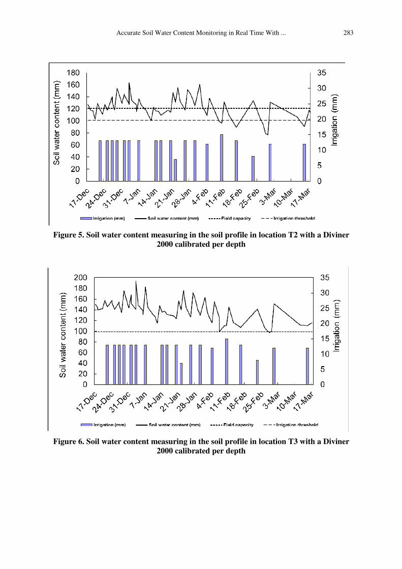
Figures 4, 5 and 6 represent soil water content on T1, T2 and T3, respectively, throughout the

summer season, measuring using the per-depth calibration. The horizontal lines on the

graphic area represent the soil water content at FC and the irrigation threshold of each.

Therefore, the area in between represents adequate soil water content, and any value above or

below represents a water excess or water deficit, respectively.

Figure 4 shows that location T1, the highest topographic location, had adequate water

content 38.1% of the time, water deficit 54% of the time and water excess for the remainder

(7.9%). This is because water easily drains to lower points in the field, especially given the

soil texture observed in soil phase 1 – sandy loam that gets coarser in depth.


Location T2 had adequate soil water content 38.7% of the time, water excess 46.8% of the

time, and water deficit for the remainder (14.5%) (Figure 5). This can be explained by the

observation point’s location at a lower topographic level, where it receives water draining

from higher points. Additionally, the soil phase of this location shows a hardpan restricting

drainage in depth: therefore, water excess does not easily clear. Thus, soil water content is

generally higher than that observed in location T1.

Location T3, at the lowest topographic point in the field and a shallower depth (0.50m), also

presents a hardpan This means that this soil profile receives water drained from the higher

topographic areas, has limited drainage due the hardpan observed and the lowest water

holding capacity of the three locations. This explains why adequate soil water content was

observed only 3.2% of the time, whereas water excess was observed for the remainder of the

time (Figure 6).

CONCLUSIONS

The probe Diviner 2000 is highly sensitive to soil water content variation per depth as well as

in the soil profile as a whole. The correlation found was better in the first 0.40m (R2>0.91)

than at 0.50 and 0.60m (R2<0.75). The calibration equation for the whole profile is

moderately precise (R2>0.81) in relation to the per-depth calibration equations. Field

calibrations were more precise than the manufacturer calibration in determining actual soil

water content per depth and across the whole profile.

When properly calibrated, the probe Diviner 2000 proves to be effective to accurately

measuring soil water content in the field in real time. When used at different points in the

field, the probe helps to detect different irrigation management needs depending on the soil

conditions of the specific location, such as water holding capacity and ability to drain.

LITERATURE CITED

[1] Anderson, S.A., C.R. Da Silva, and C. Fonseca. 2010. Calibration of Diviner 2000

capacitance probe in two soils in Piaui State, Brazil. Pp 1.5 (1-10). In: The Third

International Symposium on Soil Water Measurement Using Capacitance, Impedance and

TDT. Murcia, España, 7-9 abril, 2010. CEBAS-CSIC, Campus Universitario de Espinardo,

Murcia, España.

[2] Bryla, D. 2004. Trials Find Drip Irrigation Most Efficient for Peach Trees. Agricultural

Research Initiative. California State University. Fresno, Ca. USA. 4 p.


[3] Burgess, P.J., B.R. Reinhard, and P. Pasturel. 2006. Compatible measurements of

volumetric soil water content using a neutron probe and Diviner 2000 after field calibration.

Soil Use Management 22:401-404. DOI: 10.1111/j.1475-2743.2006.00060.x.

[4] Cassel, D. K., P.G. Kachanoski, and G.C. Topp. 1994. Practical considerations for using a

TDR cable tester. Soil Technology. 7(2): 113–126. DOI: 10.1016/0933-3630(94)90013-2.

[5] CIREN, 1996. Estudio Agrológico de la VI Región. CIREN CORFO. Santiago, Chile.

[6] Da Silva C., A. De Andrade, J. Alves, A. Barros, F. De Brito, and M. Coelho. 2007.

Calibration of a capacitance probe in a Paleudult. Scientia Agricola 64(6) 636:640.

DOI: 10.1590/S0103-90162007000600012.

[7] De Jong, R., and A. Bootsma. 1996. Review of recent developments in soil water

simulation models. Canadian Journal of Soil Science. 76(3): 263-273. DOI: 10.4141/cjss96-

033.

[8] FAO. 2003. Agricultura 21; Enfoques; Revista Gestión Moderna del Riego. Departamento

de Agricultura. FAO, Roma, Italy.

[9] Fares, A. and V. Polyakov. 2006. Advances in crop water management using capacitive

water sensors. In Sparks, D. (ed.) Advances in Agronomy. Vol. 90. Elsevier Science, USA.

pp. 43–77.

[10] Gardner, W.H. 1986. Water content. In Klute, A. et al. (eds.) Methods of Soil Analysis.

Part 1. Physical and Mineralogical Methods. 2nd Ed. ASA and SSSA, Madison, WI. pp. 493–

544.

[11] Girona, J., M. Mata, E. Fereres, D.A. Goldhamer, and M. Cohen. 2002.

Evapotranspiration and soil water dynamics of peach trees under water deficits. Agricultural.

Water Management. 54(2): 107-122. DOI: 10.1016/S0378-3774(01)00149-4.

[12] Goldhamer, D.A., E. Fereres, M. Mata, J. Girona, and M. Cohen. 1999. Sensitivity of

continuous and discrete plant and soil wáter status monitoring in peach trees subject to deficit

irrigation. Journal of the American Society for Horticultural Science 124(4): 437-444.

[13] Greancen, E.L. 1981. Soil Water Assessment by the Neutron Method. CSIRO

Melbourne, Australia.

[14] Groves S. and S. Rose. 2004. Calibration equations for Diviner 2000 capacitance

measurements of volumetric soil water content of six soils. Soil Use and Management. 20:96-

97.


[15] Haberland J., R. Gálvez, C. Kremer and C. Carter. 2014. Laboratory and field calibration

of the diviner 2000 probe in two soil. Journal of Irrigation and Drainage Engineering 140(4).

DOI: 10.1061/(ASCE).

[16] Hanson, R.B., S. Orloff, and D. Petrs. 2000. Monitoring soil moisture helps refine

irrigation management. California Agriculture. 54(3): 38-42. DOI: 10.3733/ca.v054n03p38.

[17] Hu, W., M., Shao, Q.J., Wang and K, Reichardt. 2008. Soil water content temporal-

spatial variability of the surface layer of a Loess Plateau hillside in China. Scientia Agricola

(Piracicaba, Braz.), 65(3): 277-289.

[18] Intrigliolo, D., P. Ferrer, and J.R. Castel. 2007. Monitorización del riego en la vid. p. 83-

113. In: P. Baeza, J.R. Trujillo and P. Sanchez. Fundamentos, aplicación y consecuencias del

riego en la vid. Editorial Agrícola Española. Madrid, España.

[19] Lowery, B., Datiri, B.C., and Andraski, B.J. (1986). An electrical readout system for

tensiometers. Soil Science Society of America Journal, 50(2), 494-496.

[20] Morgan K.T., Parsons, L.R., Wheaton T.A., Pitts D.J. and T.A. Obreza. 1999. Field

calibration of a capacitance water content probe in fine sand soils. Soil Science Society of

America Journal. 63(4):987-989. DOI:10.2136/sssaj1999.634987x.

[21] Muñoz-Carpena, R., Shukla, S. and K. Morgan. 2004. Field devices for monitoring soil

water content. University of Florida Cooperative Extension Service, Institute of Food and

Agricultural Sciences, EDIS.

[22] Paltineanu I., and J.L. Starr. 1997. Real time dynamics using multisensors capacitance

probes: Laboratory calibration. Soil Science Society of America Journal. 161:1576-1585.

[23] Robinson, M., and Dean, T.J. (1993). Measurement of near surface soil water content

using a capacitance probe. Hydrological Processes, 7(1), 77-86.

[24] Seyfried, M.S. 1993. Field calibration and monitoring of soil-water content with

fiberglass electrical resistance sensors. Soil Science Society of America Journal. 57: 1432–

1436.

[25] Spaans, E.J., and Baker, J.M. 1992. Calibration of watermark soil moisture sensors for

soil matric potential and temperature. Plant Soil. 143: 213–217.

[26] Topp, G., Davis J.L. and Annan, A. 1980. Electromagnetic determination of soil-water

content measurements in coaxial transmission lines. Water Resources. Research. 16(3): 574–

582. DOI: 10.1029/WR016i003p00574


Tables and Figures

Figure 1. Distribution of the access tubes for field calibration.

Figure 2. Representation of the three topographic locations of access tubes for the soil

water content measuring in real time.

T1 T2

T3


Figure 3. Soil water content estimates (mm) from different calibration equations

(manufacturer, per depth, soil profile) and the actual soil water content determined by

the gravimetric method from the six reading points evaluated (two reading points per

water content conditions)

Figure 4. Soil water content measuring in the soil profile in location T1 with a Diviner

2000 calibrated per depth.



2000 calibrated per depth


2000 calibrated per depth


Table 1. Depth, Soil series FC, PWP and Threshold of each observation point

Access tube Depth (m) Soil series phase

Soil Water Content (mm)

FC PWP 30%

Threshold

T1 0.60 1 101.00 37.85 82.06

T2 0.60 2 121.10 54.40 101.09

T3 0.50 2 99.10 42.20 82.03

Table 2. Calibration equations per depth and whole profile

Depth (m) Coefficient a Coefficient b Calibration Equation R2 RMSE

0.10 0.3130 0.3106 SF=0.3130

θw0,3106 0.9255 0.0177

0.20 0.3014 0.2988 SF=0.3014

θw0,2988 0.9143 0.0429

0.30 0.3477 0.2697 SF=0.3477

θw0,2697 0.9619 0.0320

0.40 0.4150 0.2168 SF=0.4150

θw0,2168 0.9390 0.0401

0.50 0.5294 0.1450 SF=0.5294 θw0,145 0.7342 0.0642

0.60 0.4884 0.1593 SF=0.4884

θw0,1593 0.5882 0.0780

(0-0.6 m) 0.3734 0.2470 SF=0.3734 θw0,247 0.8125 0.0467

ACCURATE SOIL WATER CONTENT MONITORING … · accurate soil water content monitoring in real time...

Documents

Transcript of ACCURATE SOIL WATER CONTENT MONITORING … · accurate soil water content monitoring in real time...