Accurate and Economical Traveling-Wave Fault Locating Without Communications

Armando Guzmán, Bogdan Kasztenny, Yajian Tong, and Mangapathirao V. Mynam, Schweitzer Engineering Laboratories, Inc.

Abstract—This paper describes a single-ended traveling-wave-based fault-locating method that works with currents only. Unlike current transformers, coupling-capacitor voltage transformers do not have a frequency bandwidth that is wide enough to allow measuring of voltage traveling waves for this application. The key to a robust single-ended traveling-wave fault-locating method is to correctly identify reflections from the fault point. For this purpose, the method uses additional information, such as the impedance-based fault location and reflections from the remote terminal and external network elements. This paper presents the single-ended traveling-wave-based fault-locating method in detail and explains how to perform fault locating manually using ultra-high-resolution fault records from any recording device. This paper also presents laboratory test results as well as field cases in which line crews found the actual faults.

I. INTRODUCTION A double-ended traveling-wave-based fault-locating

(DETWFL) method provides accurate and dependable results but requires communications to collect traveling-wave (TW) data from the two line terminals and a common time reference for these signals. In this approach, the data acquisition devices (fault locators or protective relays) send TW information to a central computer or exchange this information between the two devices via communications links to estimate the fault location (FL) autonomously without a human in the loop. These communications and common time reference requirements could limit the DETWFL method application. When communications or the time reference are not available, the user is limited to manual analysis using event records from one or two terminals to estimate the FL.

This paper describes a TW fault-locating method that works without communications (i.e., a single-ended method). Single-ended traveling-wave-based fault-locating (SETWFL) methods use multiple reflections from the fault point for FL estimation. These reflections can be confused with reflected TWs from the remote terminal of the faulted line or from the remote terminals of the adjacent lines. The key to a robust SETWFL method is to correctly identify reflections from the fault point.

References [1] and [2] discuss a successfully developed single-ended fault locator for high-voltage dc (HVdc) lines. This device uses voltage and current to separate incident and reflected TWs.

In ac systems, current TWs can be measured accurately using standard current transformers (CTs). Measuring voltage TWs—especially reflections after the initial wave—cannot be counted on due to the poor frequency response of coupling-

capacitor voltage transformers (CCVTs). As a result of the lack of voltage TW data, a SETWFL method that uses only currents faces challenges in identifying which TW reflections come from the point of the fault and which come from buses behind the line.

This paper presents a method that uses the first reflection from the fault to perform FL estimation. To identify this particular TW, the method uses reflections from the fault, the local line terminal, the remote line terminal, or the remote terminals of the adjacent lines. The method assumes several FLs based on the measured TWs.

For each assumed FL, the method uses two approaches to identify the first reflection from the fault. The repeating travel time (RTT) approach identifies all TWs traveling from the local terminal to the fault and back to the local terminal as well as TWs traveling from the fault to the remote terminal and from the remote terminal to the local terminal, passing through the fault along the way. The expected TW (ETW) approach generates a list of all expected TWs for each assumed FL and inspects how well the measured TWs match the expected TWs. With the information from the two approaches, the algorithm selects the most likely FL.

This paper also presents field cases in which the actual FL was found by the line crews and from which we can determine the fault-locating accuracy. The described SETWFL method can be applied to two-terminal lines and radial lines.

For completeness, this paper includes tutorial material on impedance- and TW-based fault-locating methods, propagation of TWs, and data acquisition and time stamping of TWs.

II. REVIEW OF FAULT-LOCATING METHODS IN POWER LINES Impedance- and TW-based fault-locating methods are the

most common methods for locating faults on power transmission lines. These fault-locating methods can be grouped under single-ended and multi-ended methods, depending on how many terminals provide measurements. In this paper, we focus on two-terminal lines and, therefore, cover double-ended methods in the more general category of multi-ended fault locators.

A. Impedance-Based Methods

1) Single-Ended Impedance-Based Method The single-ended impedance-based fault-locating method

(SEZFL) uses local voltages and currents along with the positive- and zero-sequence line impedances to estimate the FL.

Depending on the fault type, one SEZFL method uses one of the six loop measurements listed in Table I for unbalanced faults and positive-sequence voltage and current measurements (V1 and I1, respectively) for three-phase faults. This method uses (1) to estimate the FL.

( )

( )LP POL

1 LP POL

Im V • IM LL •

Im Z • I • I

∗

∗= (1)

where: M is the FL in km or mi. LL is the line length in km or mi. Z1 is the positive-sequence line impedance in Ω. VLP and ILP are the voltage and current measurements. IPOL is the polarizing current.

TABLE I CURRENT AND VOLTAGE MEASUREMENTS USED BY THE SEZFL METHOD

Fault Type Voltage (VLP) Current (ILP)

AG VA IA + (Z0 / Z1 – 1) • I0

BG VB IB + (Z0 / Z1 – 1) • I0

CG VC IC + (Z0 / Z1 – 1) • I0

AB, ABG VA – VB IA – IB

BC, BCG VB – VC IB – IC

CA, CAG VC – VA IC – IA

ABC V1 I1

In Table I, Z0 is the zero-sequence impedance of the line and I0 is the zero-sequence current.

Different SEZFL methods are derived using different polarizing currents. Negative-sequence current is our preferred choice for the polarizing current for unbalanced faults, and positive-sequence current is our preferred choice for three-phase balanced faults.

The accuracy of the SEZFL method depends on several well-known factors, including the accuracy of the line impedance data, fault resistance, system nonhomogeneity, and mutual coupling [3]. For single-line-to-ground faults in nonhomogeneous systems with high resistance, expect FL errors that are much greater than 5 percent using the SEZFL method.

2) Double-Ended Impedance-Based Method The double-ended impedance-based fault-locating (DEZFL)

method uses voltages and currents from the local and remote terminals and, therefore, requires a communications channel and a common angle reference for the local and remote phasors. One such method uses the negative-sequence voltage profile along the faulted line for all unbalanced faults. Fig. 1 shows a negative-sequence voltage profile for a fault at F on a line of length, LL. The fault is M (km or mi) away from the Local Terminal, L, and LL – M (km or mi) away from the Remote Terminal, R.

L F RM LL – M

I2RI2L

V2LV2F

V2R

Fig. 1. Negative-sequence voltage profile explaining the DEZFL method.

For unbalanced faults, the DEZFL method estimates the FL according to (2).

( )

( )2L 2R 1 2R

1 2L 2R

V – V Z • IM LL • Re

Z • I I +

= + (2)

where: V2L is the local negative-sequence voltage. V2R is the remote negative-sequence voltage. I2L is the local negative-sequence current. I2R is the remote negative-sequence current.

The DEZFL method is immune to the remote infeed effect, and it works well for resistive faults in nonhomogeneous systems. Line nonhomogeneity affects this method but to a lesser degree than it affects the SEZFL method. The DEZFL method does not use the zero-sequence line impedance and is, therefore, not affected by errors in the zero-sequence impedance data. It is also not affected by mutual zero-sequence coupling. Expect better accuracy from the DEZFL method than from the SEZFL method. However, do not expect accuracy better than about 1 to 2 percent of the line length for ground faults.

B. Traveling-Wave-Based Methods Overall, impedance-based fault-locating methods require

the presence of a fault for a couple of cycles to provide accurate results. While this requirement is not an issue in subtransmission network applications, it can be an issue in extra-high voltage (EHV) and ultra-high voltage (UHV) applications, where faults are sometimes cleared in less than two cycles. Furthermore, impedance-based methods might not be applicable to lines with series compensation or lines that are close to series compensation because the combination of a series capacitor and its overvoltage protection creates a current-dependent voltage drop (and thus series impedance) that is not accounted for in the impedance-based FL equations.

Because of the importance of locating faults to avoid fault recurrences and the high cost associated with finding line faults, utilities require accurate fault-locating devices for all applications. For this reason, some utilities have installed devices that use TW-based methods to locate faults. These methods provide accuracy on the order of one tower span.

1) Double-Ended TW Method The DETWFL method uses the first wave arrival times at

the local and remote terminals along with the line length, LL, and TW line propagation time (TWLPT) to estimate the FL.

The local and remote devices acquiring the data require a common time reference. The Bewley diagram [4], shown in Fig. 2, illustrates the arrival times at the local, tL, and remote, tR, terminals for a fault at F.

L F R

tL

tR

M LL – MtFAULT = 0

Time Time

Fig. 2. Bewley diagram explaining the DETWFL method.

The fault is M (km or mi) away from the Local Terminal, L, and LL – M (km or mi) away from the Remote Terminal, R. The TW propagation velocity, PV, for the line is LL / TWLPT. The first TW arrives at the Local Terminal, L, at tL = M / PV time. The first TW arrives at the Remote Terminal, R, at tR = (LL – M) / PV time. Solving these two equations for M, we obtain (3), which the DETWFL method uses to estimate the FL.

L Rt – tLLM 12 TWLPT

= +

(3)

We use (3) to analyze the DETWFL sensitivity to errors in settings and wave arrival time estimation. Expect the following sensitivities to errors:

• 1 percent of error in the LL setting results in 1 percent of error in the FL.

• 1 µs of error in the TWLPT setting results in a fault-locating error of 150 m (500 ft) for overhead lines and 75 m (250 ft) for underground cables.

• 1 µs of error in the TW time stamp results in a fault-locating error of approximately half the tower span in an overhead power line and half of that value in underground cables.

Expect line sag of about 0.3 percent of the line length. Changes in line sag, caused by ambient temperature changes and line loading, result in line length changes of a fraction of 0.3 percent. For this reason, expect an extra fault-locating error of a fraction of 0.3 percent.

2) Single-Ended TW Method The SETWFL method uses the time difference between the

first TW from the fault and the first reflection from the fault, measured at the local terminal [1] [2] [5] [6]. Fig. 3 shows the Bewley diagram for a fault at F on a line of length LL. The fault is M (km or mi) away from the Local Terminal, L, and LL – M (km or mi) away from the Remote Terminal, R. Consider Bus B behind the Local Terminal, L, to be a bus terminating a line connected to the Local Terminal, L. A current TW launched at the fault point F arrives at the Local Terminal, L, at t1. Part of it reflects, travels back toward the fault, reflects back from the fault, and then returns to the Local Terminal, L at t4. During the t4 – t1 time interval, the TW traveled a distance of 2 • M.

Time

tFAULT = 0

L F R

t1

t2

t3

t4

t6

MB

LL – M

Time Time

Fig. 3. Bewley diagram explaining the SETWFL method.

The method works well if it correctly identifies the first return from the fault (t4 time, in this example). The SETWFL method calculates the FL using (4) when it identifies the reflection from the fault (t4).

( )4 1t – t

M • LL2 • TWLPT

= (4)

We use (4) to analyze the sensitivity of the SETWFL method to errors in settings and wave arrival time estimation. Expect the following sensitivities to errors:

• 1 percent of error in the LL setting results in 1 percent of error in the FL.

• 1 µs of error in the TWLPT setting results in a fault-locating error of as much as 300 m (1000 ft) for overhead lines and as much as 150 m (500 ft) for underground cables.

• 1 µs of error in the TW time stamp results in a fault-locating error of approximately one tower span in an overhead power line and one-half of that value in underground cables.

It is challenging to find the TW that is the first reflection from the fault among all of the other TWs that may arrive at the local terminal, including the TWs that arrive from behind the relay (t2 in Fig. 3) or from the buses in front of the relay (t3 and t6 in Fig. 3). Section V provides details on the proposed SETWFL method with an emphasis on how to identify the first TW reflected from the fault.

While TW-based methods provide a more accurate FL estimation (on the order of one to two tower spans) than impedance-based methods, there are cases where the FL cannot be estimated. For example, faults that occur when the voltage at the FL crosses zero do not launch TWs. Protective relays that include both impedance-based and TW-based methods have the advantage of providing the FL even in cases where the TW amplitude is too low for reliable detection (e.g., faults that occur

near voltage zero). In these cases, the relays estimate the FL using the DEZFL method. If the remote measurements are not available, the relay estimates the FL using the SEZFL method, thus providing a robust FL result with the best possible accuracy under all fault, communications channels, and time and angle reference conditions.

III. PROPAGATION OF TWS A SETWFL device works with multiple TWs that often

traveled a long distance and were reflected and transmitted through a number of discontinuities. Assume a 200 mi line with a fault 150 mi away from the terminal. The first TW from the fault arrives at the terminal after traveling 150 mi. Part of it reflects back to the fault, travels another 150 mi to partially reflect from the fault, and returns back to the terminal. The first return from the fault traveled a total of 450 mi and went through two reflections. The first reflection from the remote bus of the line, also often used in SETWFL algorithms, traveled a total of 250 mi in this example. These long travel distances result in considerable dispersion and attenuation of the TWs used by SETWFL devices.

TWs reflected from the line terminals (buses) may exhibit ringing and other distortions caused by capacitances and inductances present on the bus, including inductances and capacitances of the buswork, stray capacitances of transformer windings, CCVT circuitry, and so on. In addition, very high-frequency ringing may appear in the secondary current signals because of waves traveling in the secondary cables between the CTs and the TW fault-locating device.

In order to design a robust SETWFL algorithm, we must understand and accommodate considerable TW dispersion and attenuation, as well as potential ringing and additional distortions in the measured current TWs. The remainder of this section explains the principles of attenuation, dispersion, reflection, and transmission of TWs. Section IV describes the signal processing we use to accommodate these phenomena for accurate SETWFL and DETWFL implementations.

A. Attenuation and Dispersion When a fault occurs on a transmission line, the fault

launches waves that travel from the fault to the line terminals, as Fig. 4 illustrates.

L R

x

Fig. 4. TWs launched by a fault on a transmission line.

Equation (5) represents the current TWs where the first term corresponds to the wave traveling toward the left terminal (Terminal L) and the second term to the wave traveling toward the right terminal (Terminal R) [4]. In this equation, γ is the propagation constant, which is a function of the line resistance, inductance, conductance, and capacitance; x is distance; and

ƒ1(t) and ƒ2(t) are functions that model the shape of the wave. The line resistance and inductance change because of the skin effect, and the total line capacitance is affected by the lumped capacitances of the insulators and corona [4]. All of these factors affect the magnitude and shape of the wave (the ƒ1(t) and ƒ2(t) functions).

( ) ( ) ( )x – x1 2i x, t t • e t • eγ γ= +f f (5)

As the waves travel, their magnitudes decrease; that is, they are attenuated because of energy losses caused by conductor resistance. The eγx and e–γx terms in (5) model this attenuation. The shape of the front of the TWs starts to lean instead of being a very steep step, and it starts to round at the top because of dispersion. Fig. 5 shows how the current waves propagate across a 400 kV line in response to an ideal voltage step. Notice how the shape of the TW changes as it travels along the line. The plots in Fig. 5 were obtained using an Electromagnetic Transients Program (EMTP) model that considers the skin effect [7]. The plots are shifted in time to eliminate the propagation delay and allow better comparison of the shape of the wave front.

800

600

500

400

300

0–5 5 25Time (µs)

Am

pere

s

700

200

100

010 15 20 30

Fig. 5. TW attenuation and dispersion as a wave travels along a 400 kV transmission line.

Attenuation and dispersion are caused by energy losses and variations in the line inductance and capacitance. Dispersion is of particular interest for TW fault locating because the steepness of the TW rising edge can impact the estimation of the TW arrival time.

B. Reflection and Transmission of TWs TWs arrive at junctions that join elements such as lines,

transformers, faults, and so on. Depending on the characteristic impedances of the segments connected to the junction, part of the TW arriving in one segment is reflected and travels back in that segment and part of it is transmitted and travels further in the connected segments. In this subsection, we describe the equations that determine how these TWs are reflected and transmitted when arriving at junctions with two and three segments. We can use similar equations in junctions with more segments.

1) Two-Segment Junction A fault launches waves in both directions, which propagate

from the fault toward the line terminals. These TWs appear in the voltage and current signals. The voltage and current TWs are related by the characteristic impedance of the line, ZC.

When an incident TW with current, iI, reaches a line terminal, a portion of the incident TW is transmitted, iT, and a portion is reflected, iR, as shown in Fig. 6. The portions that are transmitted and reflected depend on the characteristic impedance beyond the transition point ZT and the characteristic impedance ZC of the line the wave traveled. Keep in mind that a TWFL device at the line terminal measures current TWs that are the sum of the incident and reflected TWs.

ZC ZT

iT

iR

iI vT

Fig. 6. Illustration of the incident, iI, transmitted, iT, and reflected, iR, waves.

When a surge reaches a termination impedance, ZT, at the terminal, the voltage, vT, at the terminal equals iT • ZT. The arrival of iI and vI (voltage TW) at the terminal creates reflected TWs iR and vR, according to (6).

T I RT

T I R

v v vZ

i i i+

= =+

(6)

where vT is the terminal voltage and iT is the transmitted current.

Equation (7) relates iI and vI and (8) relates vR and iR with the characteristic impedance, ZC. Our objective is to define a relationship between iI and iR. Therefore, we substitute (7) and (8) into (6), and we obtain (9), which is the reflected TW current as a function of iI, ZC, and ZT.

IC

I

vZ

i= (7)

RC

R

vZ –

i= (8)

C TR I i I

C T

Z Zi i i

Z Z−

= = Γ+

(9)

where Γi is the current reflection coefficient. At the FL, ZT is typically less than ZC and Γi is positive.

Therefore, the incident current TW and the current TW reflected from the fault have the same polarity; we use this principle in Section V to identify the first reflection from the fault.

In (10), we express iT in terms of iI, ZC, and ZT.

CT I i I

C T

2 • Zi i i

Z Z= = Τ

+ (10)

where Τi is the current transmission coefficient.

2) Three-Segment Junction When passing through a fault or junction point with three

segments, the incident current TWs are reflected and

transmitted according to the characteristic impedances of the connected line segments (see Fig. 7). For the incident TW, i1

I, the reflection, Γi, and transmission, Ti, coefficients are calculated using (11) and (12) [4] [8].

i1I

Z1

Z3

Z2

i1R

i2T

i3T

i1I

Z1

Z3

Z2

Fig. 7. Current TW passing through a junction point.

1 Pi

1 P

Z ZZ Z

−Γ =

+ (11)

1i

1 P

2 • ZT

Z Z=

+ (12)

where Z1 is the characteristic impedance of Segment 1 and ZP is the equivalent impedance of the characteristic impedances of Segments 2 and 3 (connected in parallel), Z2 and Z3, as shown in (13).

2 3P

2 3

Z • ZZ

Z Z=

+ (13)

The reflected current, i1R, and transmitted currents, i2

T and i3

T, are calculated according to (14), (15), and (16), respectively.

R I1 i 1i • i= Γ (14)

T IP2 i 1

2

Zi T • i

Z= (15)

T IP3 i 1

3

Zi T • i

Z= (16)

The reflection and transmission coefficients determine how the TWs reflect and transmit when they reach the line terminals, fault, and elements in the external network.

IV. DATA ACQUISITION AND TW TIME STAMPING Proper detection of TWs from the raw current measurements

and the accurate time stamping of these TWs are the foundations of robust SETWFL and DETWFL systems. TW detection refers to an operation of “finding” individual TWs in the time series of raw current samples, i.e., identifying or isolating each TW and differentiating multiple TWs that arrive in quick succession. TW time stamping refers to an operation of assigning an arrival time to each TW in a way that is least dependent on the TW shape, especially:

• TW signal level (attenuation). • TW ramp-up time and rounded top (dispersion). • TW distortion (other signals present in the TW,

including any high-frequency oscillations). This section provides details on the data acquisition and

signal processing of our TWFL implementation.

A. Data Acquisition Our implementation [9] applies a data acquisition system

with the following characteristics: • Sampling rate of 1 MHz, i.e., with samples taken

every microsecond using a number of single-channel analog-to-digital converters (ADCs) with precisely synchronized sampling across all channels.

• ADC resolution of 18 bits for the full-range fault current, allowing more than sufficient resolution for the TW signal components. Note that the incident current TWs are limited by the line characteristic impedance and the system voltage and are many times lower than the full-scale fault currents. The TW currents are on the order of 1 kA for an overhead line, while the full-scale fault currents are on the order of tens of kA. Current TWs for faults at low-voltage points on waves that are further subjected to attenuation and dispersion phenomena may be as low as a few tens of primary amperes.

• Galvanic isolation of the current inputs optimized (designed and corrected) for flat frequency response in the frequency band up to approximately 400 kHz.

• Anti-aliasing filtering with cut-off frequency on the order of 400 kHz. The filter passes high-frequency signal components that the device uses to detect TWs (i.e., sharp edges in the signals), yet high-frequency ringing is possible due to short secondary CT cables and should be prevented—via analog low-pass filtering—from aliasing.

• Highly accurate and stable internal oscillator for timekeeping. The system must retain a nanosecond-level timing accuracy over a time interval on the order of 2 to 3 ms (i.e., for as long as the TWs arrive at the terminal). The implementation uses a 10 parts per million (PPM) oscillator, and the fault-locating device further disciplines the oscillator (calibrates its frequency) using an accurate satellite clock if the clock is connected to the device (optional).

B. Practical Aspects of Signal Attenuation and Dispersion From the signal processing point of view, dispersion refers

to a phenomenon where a TW launched as a step change (an ideal wave) exhibits a ramp-up time that increases with the distance traveled by the wave (see Fig. 8). Attenuation refers to a phenomenon where a TW lowers its magnitude as it travels along the line. In order to accurately and consistently capture the TW arrival time irrespective of the TW magnitude, our time-stamping algorithm uses a differentiator-smoother filter [10] with an adequately long data window.

The differentiator-smoother filter spreads the sharp change in the raw (full-scale) current into a pulse that lasts as long as the filter’s data window (see Fig. 8). The time of the peak of the differentiator-smoother output corresponds to the time of the step in the raw current, with a small time difference equal to the fixed group delay of the differentiator-smoother filter. Hence, the time of the peak of the differentiator-smoother output is not

affected by the magnitude of the step in the raw current. This filtering approach provides a simple and robust solution to attenuation, signal-loss due to transmission and reflection, and the natural variability of the TW current signal because of the voltage point-on-wave value at the FL. Also, the smoothing part of the filter attenuates any high-frequency noise (ringing) in the TW signal, as well as the impact of ADC resolution for TWs of a very small magnitude.

Distance traveled

TW signal

Raw current

Fig. 8. Explanation of dispersion and its impact on time stamping.

If the TW is a ramp rather than a step, the time of the peak of the output from the differentiator-smoother consistently points to the midpoint of the TW ramp. This means that the time stamp is slightly affected by dispersion. However, any TWFL device effectively measures a difference in the TW arrival times and compares it with the TW line propagation time (i.e., the total time it takes for a TW to travel the line length). The TW line propagation time is a setting, TWLPT. Reference [10] proves that, as long as the level of dispersion is directly proportional to the distance the TW traveled and the TW line propagation time setting is measured using the TWFL device’s time-stamping algorithm, the effect of dispersion cancels when using the differentiator-smoother algorithm to time stamp the TWs.

C. High-Frequency Signal Distortion As mentioned before, a raw current signal may exhibit high-

frequency oscillations, mainly due to ringing in the secondary CT cables. Assuming a 150 m (500 ft) CT cable length and the TW propagation velocity in the cable of 0.7 pu of the speed of light in free space, the TW propagation time in the CT cable is about 1 µs one way or 2 µs round trip. As the secondary current TW bounces between the CT secondary winding (an open circuit) and the TWFL device current input (a short circuit), it creates oscillations with periods on the order of 1 to 2 µs, as shown in Fig. 9. The parasitic capacitance of the CT secondary winding may further contribute to these high-frequency oscillations.

Our implementation uses a relatively long data window in the differentiator-smoother filter (on the order of several multiples of the expected oscillation period) to effectively suppress the high-frequency oscillations, as shown in Fig. 9. This way, the pulse at the differentiator-smoother output may be slightly distorted, but it still reliably indicates the midpoint of the TW ramp, regardless of the high-frequency oscillations that may be present in the raw current.

Time

Raw

cur

rent

Time

DS

out

put

Time

Raw

cur

rent

Time

DS

out

put

Fig. 9. The differentiator-smoother filter reduces the impact of high-frequency ringing on TW time stamping.

D. TW Detection and Validation A TWFL device must detect a number of TWs in order to

autonomously calculate the distance to the fault. The first level of TW detection is to “find” all TWs, regardless of their origin. With all TWs identified and time stamped, the TWFL algorithm uses TWs reflected from the fault, from the remote bus, and from buses of the adjacent lines to identify the first reflection from the fault (see Section V).

The differentiator-smoother filter effectively converts a steep change in the raw current into a pulse. The steeper the change, the more the differentiator-smoother output resembles a triangular shape. For TWs with dispersion (a ramp), the output resembles a parabola. In any case, a clear pulse is visible in the differentiator-smoother output for a TW in the raw current signal. Our fault-locating implementation marks a local peak of the differentiator-smoother output as a valid TW if the following conditions are true:

• The differentiator-smoother output is considerably lower before reaching a local peak and after reaching the local peak.

• The magnitude of the local peak is higher than a minimum threshold associated with the device’s capability to measure TWs.

In TW protection applications, we impose more conditions before we declare any given pulse in the differentiator-smoother output as a valid TW. In TWFL applications, however, we apply relatively relaxed conditions to identify TWs in the stream of raw current samples. This is especially important for identifying TWs that traveled a long distance and went through multiple discontinuities; these TWs are relatively small and considerably dispersed.

E. Accurate Time Stamping Through Interpolation The accuracy requirement for TW time stamping is a small

fraction of a microsecond for minimizing FL errors (see

Subsection II-B). We obtain this high accuracy by using interpolation to find the time of peak in the differentiator-smoother output [10].

With reference to Fig. 10, our implementation selects a number of data points before and after the local peak in the differentiator-smoother output and fits a parabola to these points using the least-squared errors method. The time of the peak of the best-fit parabola is the accurate time stamp we use in our fault-locating algorithm. Note that in our implementation [9], the data points are spaced every microsecond, yet the time of the peak of the best-fit parabola has a fractional microsecond part. Hence, we refer to this method as interpolation. Our experience shows that this approach provides time-stamping accuracy that is several times better than the 1 µs sampling interval. Owing to this accurate time-stamping approach, when tested under ideal conditions, the SETWFL method implemented on a hardware platform [9] yields a 90th percentile error that is considerably below 20 m (66 ft) and a median error that is less than 10 m (33 ft).

Time

DS

out

put

Accurate time stamp

Best-fit parabola

Samples

Inte

rpol

ated

tim

e of

pea

k

Fig. 10. Using interpolation to find the time of the peak with accuracy that is better than one sampling interval.

F. Mode Selection TWs couple between the faulted and healthy phases as they

travel along the line. In general, the three TWs in the phase conductors can be broken down into two sets of aerial modes (alpha and beta) and one ground mode [10]. The ground mode returns via the earth and is, therefore, highly distorted and attenuated. For this reason, we do not use the ground mode for accurate time stamping. The aerial modes have much lower dispersion and are more suitable for accurate time stamping.

The alpha mode is a good representation of the three phase TWs for ground faults. It can be calculated with references to Phases A, B, and C, assuming that Phase A, B, or C is faulted. Therefore, we have three alpha modes. Similarly, the beta mode is a good representation of the three phase TWs for phase-to-phase faults. It can be calculated assuming that Phases A and B, B and C, or C and A are faulted. Therefore, we have three beta modes. Typically, the mode with the highest magnitude among the six aerial modes is the right representation of the fault type and the TW signal launched by that fault. In our implementation, we use the mode that yields the highest initial TW magnitude.

It is important to use the same mode for all TWs that are part of the TWFL calculations. When performing manual fault

locating using TWs, keep in mind that using one mode to time stamp one TW and another mode to time stamp a different TW may create an additional timing error.

V. FAULT LOCATION ESTIMATION USING LOCAL CURRENT TWS

The SETWFL method uses the current TWs at the local terminal to estimate the FL. With reference to Fig. 11, which shows a sample fault in a sample power system configuration, we know the following:

• t2 is the arrival time of a TW that came from behind the relay and, therefore, it is not the first return from the fault.

• t3 is the arrival time of a TW that traveled from the fault to the remote terminal and from the remote terminal to the local terminal.

• t4 is the arrival time of the first TW reflected from the fault. This is the time that the SETWFL algorithm must use for correct FL estimation.

• t6 is the arrival time of a TW that traveled from the fault to the local terminal, from the local terminal to the remote terminal, and from the remote terminal back to the local terminal.

A more in-depth analysis of the Bewley diagram allows the SETWFL method to identify the first reflection from the fault. The following principles help in this analysis (see Fig. 11).

L Fault Rm 1 – mB

Time

t1

Time

R = 2 • (1 – m) • TWLPTF = 2 • m • TWLPT

“Companion” TWs that meet a known relative timing criterion

0

t2

t3

t4

t5

t6

F

R

F

R

Fig. 11. Multiple TWs must create a coherent train of TWs for a fault given the location of the line terminals.

For a fault located at distance m (per unit) from the local terminal, we expect a TW returning from the remote bus at (2 – m)•TWLPT. With the first TW arriving at m • TWLPT, the time difference is 2•(1–m)•TWLPT. In other words, a “companion TW” is expected at 2•(1–m)•TWLPT in addition to the first return from the fault arriving at 2•m•TWLPT after the first TW. We can use this companion TW to verify whether a suspected first return from the fault makes sense. The timing and polarities of the TWs at 2•m•TWLPT and 2•(1–m)•TWLPT must adequately match or else M is not the real distance to the fault.

Each reflection from a discontinuity behind the relay sends a “test TW” toward the fault. As a result, we expect to see multiple pairs of TWs spaced at exactly the same time (2•m•TWLPT). Inspecting all possible TW pairs and tabulating the time differences between them allows us to narrow down the search for the real distance to the fault; the time difference that occurs most frequently is likely to be 2•m•TWLPT.

We can expand the two examples described into a more comprehensive approach. For any suspected distance-to-fault location, the SETWFL method builds a Bewley diagram assuming at least the local and remote buses as discontinuities at known locations. The rest of this section includes implementation details of the SETWFL method.

The SETWFL method uses the amplitudes, VPKs, and time stamps, TPKs, of the TWs that the algorithm identifies as possible (valid) TW reflections within an observation window that is greater than twice the TWLPT (e.g., 2.4•TWLPT). The method considers up to 15 FL hypotheses using the polarities (obtained from VPKs) and time stamps of the valid TWs. If the reflected TW is valid and it matches the polarity of the first wave, then the TW is assumed to be one of the hypotheses (i.e., the TW is considered to be the first return from the fault point) as long as the time difference between the time stamps of this TW and the TW associated with first wave arrival is less than 2•TWLPT plus a small margin (e.g., 10 µs).

The SETWFL method also uses all available FL estimations (DETWFL, DEZFL, and SEZFL) to determine the initial FL (mINI) based on the following priorities: DETWFL, DEZFL, and SEZFL.

Based on the availability of the results from any of the above methods, the SETWFL algorithm selects the FL hypothesis as follows:

• If the DETWFL result is available, the algorithm selects the hypothesis that is closest to the DETWFL estimation; else if the DEZFL result is available, the algorithm selects the hypothesis that is closest to the DEZFL estimation; else if the SEZFL result is available and the fault is not a ground fault, the algorithm selects the hypothesis that is closest to the SEZFL estimation. If the DETWFL result is available, it is reported to the user with the highest priority. Therefore, the results of the SETWFL calculations are secondary. Yet, our implementation completes these calculations for consistent reporting from all methods available for each operating condition.

• If there is a match of any of the hypotheses with any of the above FL estimations, the algorithm sets the FL confidence level bit, TWFLCL, to logical 1. The algorithm uses this bit when selecting the best FL value from all of the available results.

If the DETWFL, DEZFL, or SEZFL (single-ended impedance-based estimation for nonground faults) result is not available or there is no match to any of the hypotheses with the FL results of these methods, the algorithm ranks the hypotheses based on the TW reflections using the RTT and ETW methods, as described in the following subsections.

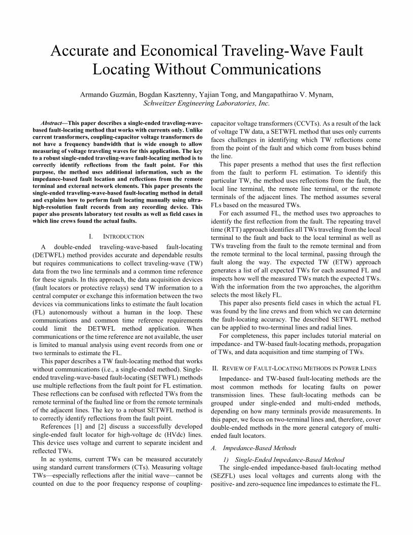
A. Repeating Travel Time (RTT) Method The RTT method uses the time difference between the

selected reflection from the fault and TPK(0) as one of the time references: F(H) = TPK(H) – TPK(0). This time reference is associated with 2•m (see Fig. 12). TPK(0) corresponds to the time associated with the first wave front from the fault; the time F shown in Fig. 12 corresponds to the time reference of the first hypothesis F(1).

m 1 – m

L R

TimeTime

...

L R

TPK(0)

...

R = 2 • (1 – m) • TWLPT

F = 2 • m • TWLPT

F

R

Fig. 12. Time references for the reflection from the fault and from the remote terminal for the first hypothesis.

For each hypothesis, the algorithm calculates another time reference using the reflection from the remote terminal that corresponds to 2•(1–m): R(H) = 2•TWLPT – F(H); the time R, in Fig. 12 corresponds to time reference R(1). We can think of that reflection from the remote terminal as a “companion.” The companion TW must arrive at the time coherent with the first wave from the fault. Fig. 12 shows the F(1) and R(1) time references of the first hypothesis.

The algorithm creates a vector, DT, that includes all of the possible time differences using all TPKs in the observation window and counts how many elements of the DT vector match F(H) and R(H) within a predefined tolerance, TWTOL1 (e.g., 10 µs) using the NM(H) and N1_M(H) counters:

• NM(H) is the number of instances that elements in DT match F(H).

• N1_M(H) is the number of instances that elements in DT match R(H).

The main benefit of the RTT method is that it takes advantage of the information provided by TWs reflected from external network elements close to the local terminal. This method uses this information when determining the number of instances, NM(H) and N1_M(H). The dashed blue traces in Fig. 13 indicate additional TWs along the line caused by a

reflection from Substation B behind the local terminal that provide information to identify the first reflection from the fault.

m 1 – m

L R

TimeTime

...

L RB

B

R

R

F

F

Fig. 13. Reflection from the external network element B provides additional information for selecting the right hypothesis.

B. Expected TW (ETW) Method For each hypothesis, the algorithm in the ETW method

determines a weighting factor, WGHT(H), and sets it to logical 1 if the reflection from the remote terminal R(H) that corresponds to the particular reflection from the fault F(H) exists (see Fig. 14). If WGHT(H) = 1, the algorithm includes the number of times that the measured TWs match the expected TWs for the particular hypothesis when ranking the hypotheses. In this instance, the algorithm also sets TWFLCL to logical 1.

L R

m

Reflection from fault

1 – m

R

Reflection from remote

terminal

F

Fig. 14. Time references for the reflection from the fault and from the remote terminal for the first hypothesis.

For each hypothesis, the algorithm creates a vector, ET, that includes all of the expected TW arrival times within the observation window, according to the following patterns:

• Pattern 1, Fault-Local-Fault-Local: Fig. 15 shows this pattern for a fault at m = 0.3 pu on a 100 mi line with TWLPT = 537 µs. The time difference between the dashed lines is TWLPT.

Fig. 15. Expected arrival times (red asterisk mark) for the TW traveling from the fault to the local terminal and the reflected TWs traveling from the fault to the local terminal.

• Pattern 2, Fault-Remote-Fault-Local: Fig. 16 shows this pattern.

Fig. 16. Expected arrival times (blue asterisk mark) for TWs traveling from the fault to the remote terminal and from the remote terminal to the local terminal.

• Pattern 3, Local-Fault-Remote-Fault-Local: Fig. 17 shows this pattern.

Fig. 17. Expected arrival times (magenta asterisk mark) for TWs traveling from the local terminal to the remote terminal and from the remote terminal to the local terminal.

• Pattern 4, Local-Fault-Remote-Fault-Remote-Fault-Local: Fig. 18 shows this pattern.

Fig. 18. Expected arrival times (green asterisk mark) for TWs traveling from the local terminal to the remote terminal, from the remote terminal to the fault, from the fault to the remote terminal, and from the remote terminal to the local terminal.

Fig. 19 shows the expected TW arrival times for all of the above patterns (fault at m = 0.3).

Fig. 19. Expected TW arrival times (all asterisk marks) for a fault at m = 0.3 on a line with a line propagation time of 537 µs.

The algorithm counts how many of the measured time stamps, TPKs, match the elements of the ET vector within a predefined tolerance, TWTOL2 (e.g., 5 µs), using the NS(H) counter; NS(H) is the number of instances that measured time stamps, TPKs, match the elements in vector ET.

C. Determining the SETWFL Result When the fault is close to the local terminal, the first

reflections to arrive to the local terminal are the reflections from the fault. When the fault is close to the remote terminal, the first reflections to arrive to the local terminal are the reflections from the remote terminal. For this reason, the algorithm divides the line into three sections to determine the SETWFL result:

• Section 1: 0 <= mINI < 0.3 pu. • Section 2: 0.3 <= mINI <= 0.7 pu. • Section 3: 0.7 < mINI <= 1 pu. With the initial fault location, mINI, information, the

algorithm identifies the faulted section and orders the hypotheses in descending order as follows:

• If the fault is in Section 1, the algorithm orders the hypotheses using NM(H).

• If the fault is in Section 2, the algorithm orders the hypotheses using N(H), where:

( ) ( ) ( ) ( )N H NM H N1_ M(H) NS H • WGHT H= + + (17)

• If the fault is in Section 3, the algorithm orders the hypotheses using N1_M(H).

If mINI is not available, the algorithm assumes that mINI=0.5 pu.

After all of the hypotheses are ordered, the algorithm uses the time difference F(H) in (4) to calculate the FL for each hypothesis.

D. Selecting the Best Fault Location Result in a Fault Locator That Uses Multiple Methods

One particular fault locator [9] selects the most accurate FL based on the available results from the four methods for a given

application and operating conditions according to the following priorities:

• The DETWFL method has the highest priority. • The SETWFL method has the second highest priority

as long as the confidence level flag, TWFLCL, is set to logical 1; otherwise, it has a lower priority than the SEZFL method. This supervision ensures that the SETWFL method provides the correct FL result.

• The DEZFL method has the third highest priority. • The SEZFL method has the lowest priority. The Appendix provides a detailed example of the procedure

that the SETWFL method follows to estimate the FL when results of the other methods are not available.

In general, the DETWFL method has an extra source of error when compared with the SETWFL method and, therefore, it is generally expected to be less accurate. This error is the timing error between the fault-locating devices at both terminals of the line. When the time reference is provided via satellite clocks, it is not unusual to expect 1 µs of error at each terminal of the line. In addition, most satellite clocks do not provide for compensation of the antennae or IRIG-B cable propagation times, potentially creating yet another source of error. With a total timing error potentially as high a 2 µs, the DETWFL method may have an additional error of one tower span. On the other hand, the SETWFL method exhibits time-stamping errors because of potentially large signal distortion caused by the long distance traveled by the TWs. The DETWFL method time-stamps only the very first TWs and is not exposed that much to this error.

In one particular implementation [9], we use a direct fiber-optic channel to synchronize two relay clocks without relying on satellite clocks. Our time synchronization accuracy is better than 80 ns. As a result of such small timing errors, the DETWFL method in this particular implementation [9] is more accurate than the SETWFL method. The time-stamping errors due to distortion in the SETWFL method are higher than the clock timing errors in the DETWFL method. For this reason, in our implementation, we give the DETWFL fault-locating method priority over the SETWFL method.

DETWFL applications with less-accurate timing, such as those using satellite clocks, may have a lower accuracy than SETWFL methods.

VI. FAULT LOCATION ACCURACY ANALYSIS We analyzed the accuracy of the SETWFL method

assuming that the other methods do not provide any FL results to initialize the SETWFL method. Therefore, the SETWFL method estimates the FL using only local currents. We used relays that include this method to determine the FL. We performed laboratory tests using current signals from a power system model with the ability to simulate power system transients. We also used the currents captured by these relays in the field to estimate the FL and compared the results with the FLs provided by the line crews.

A. Laboratory Testing We modeled the power system shown in Fig. 20 using an

EMTP to evaluate the SETWFL method. The line is 100 mi long, and the system nominal operating voltage is 525 kV. The corresponding TWLPT for this line is 537 μs. There are 25 mi, double-circuit lines behind Terminals L and R of the 100 mi line. We applied an A-phase-to-ground (AG) fault at 30 mi from Terminal L on the 100 mi line. We used a low-level signal test source to apply the voltage and current signals to the relays at Terminals L and R.

EL L ERR

25 mi 25 mi

30 mi 70 mi

Fig. 20. EMTP power system model with an AG fault at 30 mi from Terminal L to evaluate the SETWFL method.

Fig. 21 shows the phase currents captured by the relay at Terminal L, and Fig. 22 shows the corresponding alpha current TWs with the reflections from the fault.

4000

3000

2000

1000

0

–1000

–2000

–3000

–4000–30 –20 –10 0 10 20 30 40

Milliseconds

Ampe

res

Fig. 21. Phase currents recorded by the relay at Terminal L.

1000

500

0

–500

–1000

0 0.2 0.4 0.6 0.8 1 1.2Milliseconds

Am

pere

s

First reflected TW from fault point

Fig. 22. Alpha current TWs at Terminal L, and the reflection from the fault that the method identified to estimate the FL.

The algorithm selected the alpha-A current, which is the maximum alpha current. Fig. 23 shows the selected alpha-A current TW and its Bewley diagram; notice that the time, t = 0, is the time of the fault (it is not the time of the arrival of the first TW at the local terminal). The relay at Terminal L reported the SETWFL at 29.934 mi. The Appendix provides details on how the device calculates the FL.

Fig. 23. Alpha-A current TW at Terminal L and associated Bewley diagram.

B. Field Cases

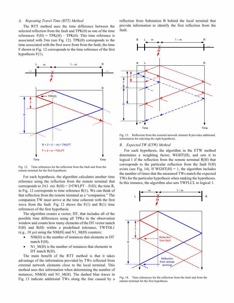
1) B-Phase-to-Ground Fault on a 161 kV Line Bonneville Power Administration (BPA) owns and operates

the Goshen and Drummond substations in Idaho. The Goshen-Drummond 161 kV line is 72.8 mi long, and its estimated TW propagation time is 395.47 μs. Fig. 24 illustrates the Goshen-Drummond line. Reference [11] shares more details about this line and our past experience with TW fault locating on this particular line using a DETWFL method and implementation.

161 kV115 kV

Goshen

DrummondMacks

Inn Madison

Targhee

Teton

72.8 mi

Swan Valley

Green Timber

Cattle Creek Palisades

26.8 mi 10.95 mi

17.99 mi

17.48 mi

46.46 mi

20.96 mi 30.82 mi

6.5 mi 31.26 mi 17.12 mi

RR RR

Fig. 24. Relays with TWFL capabilities installed on BPA’s Goshen-Drummond line.

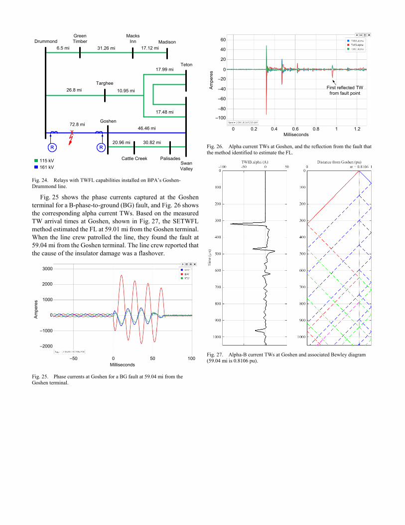
Fig. 25 shows the phase currents captured at the Goshen terminal for a B-phase-to-ground (BG) fault, and Fig. 26 shows the corresponding alpha current TWs. Based on the measured TW arrival times at Goshen, shown in Fig. 27, the SETWFL method estimated the FL at 59.01 mi from the Goshen terminal. When the line crew patrolled the line, they found the fault at 59.04 mi from the Goshen terminal. The line crew reported that the cause of the insulator damage was a flashover.

3000

1000

0

–1000

–2000

–50 0 50 100Milliseconds

Am

pere

s

2000

Fig. 25. Phase currents at Goshen for a BG fault at 59.04 mi from the Goshen terminal.

60

20

0

–20

–40

0.20 0.4 1.2Milliseconds

Ampe

res

40

–60

–80

–100

0.6 0.8 1

First reflected TW from fault point

Fig. 26. Alpha current TWs at Goshen, and the reflection from the fault that the method identified to estimate the FL.

Fig. 27. Alpha-B current TWs at Goshen and associated Bewley diagram (59.04 mi is 0.8106 pu).

RR

MPD

MPS

CTS MID

IBD CHM

TMD TYS OJP

PBD

TCL

TMT

JUI

EDO SVC

223.8 km

33.6 km 195.2 km 102 km 125 km

20 km

5.6 km

144 km

RR

Fig. 28. Relays with the SETWFL algorithm are installed at the MID and TMD terminals in the CFE 400 kV transmission network.

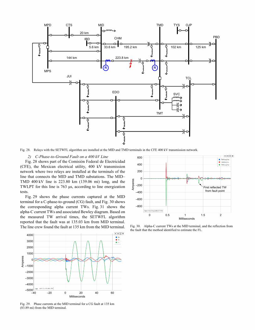
2) C-Phase-to-Ground Fault on a 400 kV Line Fig. 28 shows part of the Comisión Federal de Electricidad

(CFE), the Mexican electrical utility, 400 kV transmission network where two relays are installed at the terminals of the line that connects the MID and TMD substations. The MID–TMD 400 kV line is 223.80 km (139.06 mi) long, and the TWLPT for this line is 763 μs, according to line energization tests.

Fig. 29 shows the phase currents captured at the MID terminal for a C-phase-to-ground (CG) fault, and Fig. 30 shows the corresponding alpha current TWs. Fig. 31 shows the alpha-C current TWs and associated Bewley diagram. Based on the measured TW arrival times, the SETWFL algorithm reported that the fault was at 135.03 km from MID terminal. The line crew found the fault at 135 km from the MID terminal.

4000

3000

2000

1000

0

–1000

–2000

–3000

–4000

–20 0 20 6040Milliseconds

Ampe

res

–5000–40

Fig. 29. Phase currents at the MID terminal for a CG fault at 135 km (83.89 mi) from the MID terminal.

600

200

0

–200

–400

0.50 1Milliseconds

Ampe

res

400

–600

–800

1.5 2

First reflected TW from fault point

Fig. 30. Alpha-C current TWs at the MID terminal, and the reflection from the fault that the method identified to estimate the FL.

Fig. 31. Alpha-C current TW at the MID terminal and associated Bewley diagram (135 km [89.89 mi] is 0.6032 pu).

VII. CONCLUSION TW-based fault locators are accurate to within a tower span

and offer great operational benefits by reducing the time and cost of repairing for permanent faults and preventing reoccurrence of faults.

Double-ended TW fault locators use a simple operating principle but require communications and a common time reference. They are more expensive to apply and are exposed to more sources of errors or failure modes.

Single-ended TW fault locators eliminate the need for the communications channel and common time reference, but their operating principle is more complex.

This paper describes a practical SETWFL method that uses only local line currents. This method uses the impedance-based FL results to find the approximate FL and refines the approximation using TW measurements. This method also works if the impedance-based FL information is not available by analyzing multiple TWs for consistency in order to correctly identify the first reflection from the fault in a train of TWs.

The SETWFL method takes advantage of the fact that many TWs arriving at the line terminal provide information to identify the first reflection from the fault, including TWs reflected from network elements external to the line.

The method has been implemented in a protective relay and provides FL results autonomously without the need for a human operator. The method can be applied manually using high-resolution oscillography records from a device that does not provide single-ended fault locating.

Instrumental FL errors obtained with state-of-the-art TWFL devices are on the order of 20 m (66 ft) or less. These devices’ errors are a negligible part of the total error in which the

application factors, such as accuracy of the line length or TW line propagation time data, play a bigger role. Strive to set these parameters as accurately as possible in the fault-locating device or when performing manual calculations.

VIII. APPENDIX: FAULT LOCATION ESTIMATION EXAMPLE This example describes the steps that the SETWFL method

follows for FL estimation when none of the FL estimations from other methods are available. In this example, the power system model consists of a 100 mi, 525 kV transmission line, with 25 mi parallel lines connected to the two-line terminals and two sources behind the parallel lines, as Fig. 32 shows.

Fig. 32. 525 kV power system model with a fault at 30 mi from Terminal L.

Fig. 33 shows the alpha TW secondary currents for an AG fault at 30 mi from Terminal L on the 100 mi line. The fault occurs when the absolute value of the voltage at the FL is at its maximum. The TW line propagation times of the faulted line and the adjacent lines are 537 µs and 134.25 µs, respectively. The callouts on the A-phase current shown in Fig. 33 indicate the arrival time of the first wave, the first reflection from the fault, and the first reflection from the remote terminal. The red dots indicate valid TWs of the differentiator-smoother output, VAL, for FL estimation.

Fig. 33. Alpha TW secondary currents for an AG fault 30 mi from Terminal L and valid VAL TWs.

A. Amplitudes and Time Stamps of Valid TWs Table II shows the signed amplitudes (VPKs) and time

stamps (TPKs) of the alpha-A secondary current within an observation window of 2.4•TWLPT (e.g., 2.4•537 = 1289 µs). The algorithm identifies 12 TWs for this fault.

TABLE II SIGNED AMPLITUDES AND TIME STAMPS OF VALID TWS FOR THE AG FAULT

Index VPK TPK (µs)

0 5.519 0

1 –3.540 267.765

2 0.872 321.488

3 –1.105 535.564

4 –2.462 589.201

5 –0.877 750.446

6 0.562 857.167

7 –0.575 910.597

8 2.767 1018.131

9 0.526 1124.637

10 0.854 1178.429

11 -0.472 1285.840

Using the signed values of VPK, the algorithm selects the TWs with the same sign as the first wave from the fault within an observation window equal to 2•TWLPT + 10 µs (1084 µs). In this case, there are three hypotheses with the following time stamps: 321.488, 857.167, and 1018.131. Table II shows the VPK and TPK values of the three hypotheses in red.

B. RTT Method Based on the time stamps of the measured TWs, the

algorithm creates the following time differences vector, DT: DT = [53.430, 53.637, 53.722, 53.792, 106.506, 106.721,

107.411, 107.534, 160.152, 160.298, 160.964, 161.203, 161.244, 214.039, 214.076, 214.882, 267.470, 267.685, 267.709, 267.714, 267.765, 267.799, 267.832, 267.966, 321.262, 321.396, 321.436, 321.486, 321.603, 374.191, 375.033, 375.243, 427.983, 428.673, 428.930, 428.958, 482.567, 482.680, 535.394, 535.435, 535.564, 535.680, 589.073, 589.110, 589.201, 589.228, 589.402, 642.832, 642.865, 696.639, 696.643, 750.276, 750.366, 750.446, 803.150, 856.871, 856.942, 857.167, 910.5972, 910.664, 964.352, 1018.075, 1018.131, 1124.637, 1178.429, 1285.840]

Table III shows the time references using the first reflection from the fault F(H) and the first reflection from the remote terminal R(H) for each hypothesis. For example, the time references for the first hypothesis are F(1) = 321.488 and R(1) = 2•537 – 321.488 = 752.512 µs. For illustration, the elements in green match F(1) and the elements in blue match R(1). Therefore, NM(1) = 5 and N1_M(1) = 3. Table III also shows the number of elements in the DT vector that match the F(H) and R(H) time references within, TWTOL1 (e.g., 10 µs).

TABLE III TIME REFERENCES AND NUMBERS OF MATCHING INSTANCES

Hyp. F(H) [µs] R(H) [µs] NM(H) N1_M(H)

1 321.488 752.512 5 3

2 857.167 216.833 3 3

3 1018.167 55.869 2 4

C. Expected TW Method Table IV shows the TPK vector and the vectors of the

expected TW arrival times, ETs, for the three hypotheses. The expected times corresponding to F(H) are shown in blue, and the expected times corresponding to R(H) are shown in red.

TABLE IV EXPECTED TW ARRIVAL TIMES FOR EACH HYPOTHESIS

Index TPK (µs) ET(1) [µs] ET(2) [µs] ET(3) [µs]

0 0 0 0 0

1 267.765 321.488 216.833 55.869

2 321.488 642.975 433.666 111.738

3 535.564 752.512 650.499 167.607

4 589.201 964.462 857.167 223.476

5 750.446 1074.000 867.331 279.345

6 857.167 1285.950 1074.000 335.214

7 910.597 1084.165 391.083

8 1018.131 446.952

9 1124.637 502.822

10 1178.429 558.691

11 1285.840 614.560

12 670.429

13 726.298

14 782.167

15 838.036

16 893.905

17 949.774

18 1005.643

19 1018.131

20 1061.512

21 1074.000

22 1117.381

23 1129.869

24 1173.250

25 1229.119

26 1284.988

1) Expected and Measured TWs In Fig. 34, the red bars are the graphical representation of

the expected arrival times, including the TWTOL2 tolerance (e.g., 5 µs), and the black dots correspond to the measured TWs, TPKs. The algorithm counts the number of instances that

the measured time stamps are within the expected arrival times for each hypothesis, NS(H). The blue circles in Fig. 34 encompass the matches among TPKs and ETs. In this example, NS(1) = 3, NS(2) = 1, and NS(3) = 2.

Fig. 34. Hypothesis 1 has three instances where measured time stamps are within the expected arrival times.

2) Weighting Factor The algorithm identifies whether there is a match between

R(H) and F(H) within the TWTOL1 tolerance (e.g., 10 µs) for each hypothesis. For example, F(1) = 321.488 µs and R(1) = 755.902 µs for the first hypothesis. The algorithm finds that the sixth measured TW (TPK(5) = 750.466 µs) matches R(1) within the specified tolerance (TPK(5) is highlighted in green in Table IV). Therefore, the weighting factor for the first hypothesis is set to one, WGHT(1) = 1. Table V shows the weighting factor (WGHT) for each hypothesis and the number of instances where the TPKs match ETs.

TABLE V TIME REFERENCES AND NUMBERS OF MATCHES

Hyp. F(H) [µs] R(H) [µs] WGHT NS(H)

1 321.488 752.512 1 3

2 857.167 216.833 0 1

3 1018.131 55.869 0 2

3) Determining the SETWFL Result Assuming that there are no FL results from the other FL

methods, the algorithm identifies Section 2 as the faulted section (refer to Section V.C), mINI = 0.5 is the initial guess. For faults in Section 2, the algorithm uses (17) to obtain N(H) and order the hypotheses in descending order. Table VI shows the values of NM(H), N1_M(H), NS(H), WGHT(H), and N(H) for the three hypotheses.

TABLE VI NUMBERS OF MATCHING INSTANCES AND WEIGHTING FACTOR

Hyp. NM(H) N1_M(H) NS(H) WGHT N(H)

1 5 3 3 1 11

2 3 3 1 0 6

3 2 4 2 0 6

Based on N(H), the algorithm identifies the first hypothesis as the correct hypothesis and calculates the FL as follows:

( ) ( )F 1LL 100 321.488FL 1 • • 29.934 mi2 TWLPT 2 573

= = =

which corresponds to m = 0.299 pu. Fig. 35 shows the expected TW reflections based on the four

patterns for m = 0.299 and the TPK measurements (black circles). We can observe the match of the first reflection from the fault and the first reflection from the remote terminal with the third and sixth measured TWs, respectively. Notice that in Fig. 35, the time reference is the instant of the fault.

Fig. 35. Time stamps of the expected reflections and measured TWs for a fault at m = 0.299 on a line with TWLPT = 537 µs.

IX. ACKNOWLEDGMENT The authors thank Mr. Stephen Marx from Bonneville

Power Administration and Mr. Rafael Martínez Morales from Comisión Federal de Electricidad for providing the field data.

X. REFERENCES [1] M. Ando, E. O. Schweitzer, III, and R. A. Baker, “Development and

Field-Data Evaluation of Single-End Fault Locator for Two-Terminal HVDC Transmission Lines, Part I: Data Collection System and Field Data,” IEEE Transactions on Power Apparatus and Systems, Vol. PAS-104, Issue 12, December 1985, pp. 3524–3530.

[2] M. Ando, E. O. Schweitzer, III, and R. A. Baker, “Development and Field-Data Evaluation of Single-End Fault Locator for Two-Terminal HVDC Transmission Lines, Part II: Algorithm and Evaluation,” IEEE Transactions on Power Apparatus and Systems, Vol. PAS-104, Issue 12, December 1985, pp. 3531–3537.

[3] E. O. Schweitzer, III, “A Review of Impedance-Based Fault Locating Experience,” proceedings of the Northwest Electric Light & Power Association Conference, Bellevue, WA, April 1988.

[4] L. V. Bewley, Traveling Waves on Transmission Systems. Dover Publications, New York, NY, 1963.

[5] M. Aurangzeb, P. A. Crossley, and P. Gale, “Fault Location on a Transmission Line Using High Frequency Travelling Waves Measured at a Single Line End,” proceedings of the 2000 IEEE Power Engineering Society Winter Meeting, Vol. 4, Singapore, January 2000, pp. 2437–2442.

[6] X. Dong, Z. Chen, X. He, K. Wang, and C. Luo, “Optimizing solution of fault location,” proceedings of the 2002 IEEE Power Engineering Society Summer Meeting, Vol. 3, Chicago, IL, July 2002, pp. 1113–1117.

[7] P. Moreno, P. Gómez, J. L. Naredo, and J. L. Guardado, “Frequency Domain Transient Analysis of Electrical Networks Including Non-linear Conditions,” International Journal of Electrical Power & Energy Systems, Vol. 27, Issue 2, February 2005, pp. 139–146.

[8] A. Greenwood, Electrical Transients in Power Systems. 2nd ed. Wiley Interscience, New York, NY, 1991.

[9] SEL-T400L Instruction Manual. Available: https://selinc.com. [10] E. O. Schweitzer, III, A. Guzmán, M. V. Mynam, V. Skendzic,

B. Kasztenny, and S. Marx, “Locating Faults by the Traveling Waves They Launch,” proceedings of the 67th Annual Conference for Protective Relay Engineers, College Station, TX, March 2014.

[11] S. Marx, B. K. Johnson, A. Guzmán, V. Skendzic, and M. V. Mynam, “Traveling Wave Fault Location in Protective Relays: Design, Testing, and Results,” proceedings of the 16th Annual Georgia Tech Fault and Disturbance Analysis Conference, Atlanta, GA, May 2013.

XI. BIOGRAPHIES Armando Guzmán received his BSEE with honors from Guadalajara Autonomous University (UAG), Mexico. He received a diploma in fiber-optics engineering from Monterrey Institute of Technology and Advanced Studies (ITESM), Mexico, and his masters of science and PhD in electrical engineering and masters in computer engineering from the University of Idaho, USA. He served as regional supervisor of the Protection Department in the Western Transmission Region of the Federal Electricity Commission (the electrical utility company of Mexico) in Guadalajara, Mexico for 13 years. He lectured at UAG and the University of Idaho in power system protection and power system stability. Since 1993 he has been with Schweitzer Engineering Laboratories, Inc. in Pullman, WA, where he is a fellow research engineer. He holds numerous patents in power system protection and metering. He is a senior member of IEEE.

Bogdan Kasztenny is Senior Director, protection technology, in R&D at Schweitzer Engineering Laboratories, Inc. He has over 25 years of expertise in power system protection and control, including 10 years of academic career and 15 years of industrial experience, developing, promoting, and supporting many protection and control products. Bogdan is an IEEE Fellow, Senior Fulbright Fellow, Canadian representative of CIGRE Study Committee B5, registered professional engineer in the province of Ontario, and an adjunct professor at the University of Western Ontario. Bogdan serves on the Western Protective Relay Conference Program Committee (since 2011) and on the Developments in Power System Protection Conference Program Committee (since 2015). Bogdan has authored about 200 technical papers and holds 30 patents.

Yajian Tong received both his bachelor’s and master’s degrees in electrical engineering. He is currently an associate research engineer with Schweitzer Engineering Laboratories, Inc., in Pullman, WA. He is a member of IEEE. His interests include power system transients, power system modeling, power system protection, and power electronics.

Mangapathirao V. Mynam received his MSEE from the University of Idaho in 2003 and his BE in electrical and electronics engineering from Andhra University College of Engineering, India, in 2000. He joined Schweitzer Engineering Laboratories, Inc. (SEL) in 2003 as an associate protection engineer in the engineering services division. He is presently working as a principal research engineer in SEL research and development. He was selected to participate in the U. S. National Academy of Engineering (NAE) 15th Annual U. S. Frontiers of Engineering Symposium. He is a senior member of IEEE and holds patents in the areas of power system protection, control, and fault location.

20180221 • TP6808