Journal of Geodesy manuscript No.DOI: 10.1007/s00190-015-0868-3

Accuracy of Ionospheric Models used in GNSS and SBAS:Methodology and Analysis

A. Rovira-Garcia · J.M. Juan · J. Sanz ·G. Gonzalez-Casado · D. Ibanez

Received: May 29, 2015 / Accepted: October 19, 2015

Abstract The characterization of the accuracy of iono-

spheric models currently used in Global Navigation Satel-

lite Systems (GNSSs) is a long-standing issue. The char-

acterization remains a challenging problem owing to the

lack of sufficiently accurate slant ionospheric determi-

nations to be used as a reference. The present study

proposes a methodology based on the comparison of

the predictions of any ionospheric model with actual

unambiguous carrier-phase measurements from a global

distribution of permanent receivers. The differences are

separated as hardware delays (a receiver constant plus a

satellite constant) per day. The present study was con-

ducted for the entire year of 2014; i.e., during the last

solar cycle maximum. The ionospheric models assessed

are: the operational models broadcast by the Global

Positioning System (GPS) and Galileo constellations,

the Satellite Based Augmentation System (SBAS) (i.e.,

European Geostationary Navigation Overlay System (EG-

NOS) and Wide Area Augmentation System (WAAS)),

a number of post-process Global Ionospheric Maps (GIMs)

from different International GNSS Service (IGS) Analysis

Centres (ACs) and, finally, a more sophisticated GIM

computed by the group of Astronomy and GEomatics

This work was partially sponsored by the European SpaceAgency (ESA) Networking/Partnering Initiative (NPI) withthe industrial partner FUGRO. The Technical University ofCatalonia (UPC) contributed with an FPI-UPC grant. Workwas conducted within the ESA/ICASES project.

A. Rovira-Garcia · J.M. Juan · J. Sanz ·G. Gonzalez-Casado · D. IbanezResearch Group of Astronomy and Geomatics (gAGE)Technical University of Catalonia (UPC)Barcelona, SpainE-mail: adria.rovira@upc.edu

(gAGE). Ionospheric models based on GNSS data and

represented on a grid (IGS-GIMs or SBAS) correct about

85% of the total slant ionospheric delay, whereas the

models broadcast in the navigation messages of GPS

and Galileo only account for about 70%. Our gAGE

GIM is shown to correct 95% of the delay. The pro-

posed methodology appears to be a useful tool to im-

prove current ionospheric models.

Keywords · Ionospheric modeling · GPS · Galileo ·EGNOS · WAAS · IGS

1 Introduction

The ionosphere is a partially ionized region of the up-

per atmosphere. A large number of models are cur-

rently used to describe the delay that it produces for

electromagnetic signals propagating from satellites to

receivers. When this delay is not properly corrected,

navigation based on Global Navigation Satellite System

(GNSS) radio signals can be severely degraded. Indeed,

the performance of Standard Point Positioning (SPP)

depends on, among other factors, the capability of the

particular ionospheric model chosen to correct the GNSS

measurements.

It is relevant to characterise the accuracy of iono-

spheric models and several such attempts have been

made. For instance, simulation data sets have been ex-

tensively used to assess model performances (see Bust

and Mitchell, 2008, and references therein). Although

simulations accurately reproduce the climatological be-

haviour of the ionosphere, their degree of realism is

limited when reproducing perturbed (i.e., non-smooth)

conditions. Ionospheric gradients associated with events

2 A. Rovira-Garcia, J.M. Juan, J. Sanz, G. Gonzalez-Casado, D. Ibanez

that are quite ordinary such as geomagnetic storms at

high latitudes or equatorial plasma depletions after the

local sunset are difficult to simulate realistically.

Another common procedure is to use measurements

of the Total Electron Content (TEC), available from

dual-frequency space-borne radar altimeters such as TOPEX/Jason

(Fu et al, 1994). Although some assessments have used

these independent data (e.g. Orus et al, 2003), there are

practical disadvantages to these assessments. First, the

orbit height of such satellites is about 1,300 kilometres,

and it is thus not possible to sample the upper con-

tribution to the ionospheric delay. The plasmasphere

extends up to three Earth radii; i.e., thousands of kilo-

metres above the Low Earth Orbit (LEO) satellite. This

can contribute up to 10 Total Electron Content Units

(TECUs) (where 1 TECU = 1016 e−/m2 and corre-

sponds to 16 cm at the L1 frequency) to the total delay

(Lee et al, 2013; Gonzalez-Casado et al, 2015). Second,

biases of the satellite altimeter are not well calibrated,

and can be greater than 5 TECUs (Jee et al, 2010).

Third, the radar altimeter measurements are limited to

ice-free oceans (i.e., far from the GNSS receivers) and

have a level of noise that is several times greater than

the carrier-phase GNSS measurements (Imel, 1994). It

is thus difficult to distinguish which part of the error is

due to the ionospheric model under test and which is

due to the radar–altimeter data used as a reference. Fi-

nally, it must be noticed that the sounding of the LEO

is restricted around its orbit plane, which is almost fixed

in a Local Time (LT) and latitude frame. Indeed, the

footprint of the LEO at an specific LT occurs nearly at

the same latitude, being the sounding always limited to

this small portion of the ionosphere.

In this work, we use actual (i.e., not simulated) dual-

frequency GNSS code and carrier-phase measurements

from 150 receivers distributed worldwide. From these

data, a strategy is outlined to derive ionospheric de-

lay estimates accurate at the level of a few tenths of

1 TECU (i.e., a few centimetres). These determina-

tions are accurate enough to be used as a reference with

which to assess current ionospheric models, whose ac-

curacy is more than an order of magnitude worse.

The present paper is organized as follows. Section 2

presents a procedure with which to characterise the ac-

curacy of any ionospheric model tailored for GNSS ap-

plications. Section 3 cross-checks the method by analysing

the accuracy of different measurements potentially used

as a reference. Section 4 describes the ionospheric mod-

els assessed for the year 2014. Results of global iono-

spheric models are presented in Section 5. A regional

assessment focused on Europe and North America is

presented in Section 6. The final section summarises

the results.

2 Ionospheric Test Description

In this section, we propose a methodology that charac-

terises the accuracy of any ionospheric model used for

satellite-based navigation. The assessment requires ac-

tual, dual-frequency, unambiguous, undifferenced carrier-

phase measurements1. The method is described next.

First, the non-dispersive part of the carrier-phase

measurements is accurately modelled to the centimetre

level (refer to chapter 7 in Misra and Enge, 2001). A

global network of receivers is used to estimate a set of

parameters referred to as geodesy estimates: the station

and receiver clocks biases, zenith tropospheric delays,

and carrier-phase ambiguities.

In this geodetic processing, the Double Difference

(DD) of the ambiguities are constrained to their inte-

ger values in a sequence that starts by the wide-lane

ambiguity (BW = (f1B1− f2B2)/(f1 − f2)) using the

Melbourne Wubbena combination of code and carrier-

phases measurements (Wubbena, 1988). Once fixed the

BW , the B1 ambiguity is fixed when the floated esti-

mate of the ionosphere-free ambiguity (BC = (f21B1−f22B2)/(f21 − f22 )) is accurate enough. Finally, after fix-

ing the BW and B1 ambiguities, the ionosphere-free

ambiguityBC (or any other combination) is determined.

More details can be found in chapter 6.3 of Sanz et al

(2013).

With such constrain, any ambiguity involved in a

fixed DD can be expressed as an integer value plus a

bias for the satellite and other for the receiver (regard-

less of the arc). These biases are shared by all the obser-

vations from a specific receiver or satellite. This proce-

dure strengthens the estimation of the different param-

eters in the geodetic filter (see Laurichesse and Mercier,

2007; Mervart et al, 2008; Collins et al, 2008; Ge et al,

2008; Juan et al, 2012, among others). The resulting un-

differenced unambiguous measurements obtained using

this approach are the most accurate references available

(few millimetres) for the proposed test.

Second, the accuracy of the previous geodesy (i.e.,

non-dispersive) estimates (BW,BC) is transferred to

1 The measurements are corrected from the receiver andsatellite antenna phase centres and satellite wind up.

Accuracy of Ionospheric Models used in GNSS and SBAS: Methodology and Analysis 3

the dispersive combinations of observables, (see Hernandez-

Pajares et al, 2002, and references therein). This ap-

proach is also referred to as integer levelling (see Banville

et al, 2013). Therefore, the undifferenced carrier-phase

ambiguity in the geometry-free combination (BI = B1−B2) is built from the undifferenced BW and BC am-

biguities which have been fixed in DD mode, using the

relation

BI =1

αw(BW −BC), (1)

where the frequency factor αw = (f1f2)/(f21−f22 ) is 1.98

when Global Positioning System (GPS) frequencies L1

and L2 are used.

Third, the BI ambiguity (which has been obtained

without any ionospheric a priori information) is sub-

tracted from the geometry-free combination of carrier-

phase measurements (LI = L1 − L2) (see Lanyi and

Roth, 1988). In this manner, a very precise sample of

the actual Slant Total Electron Content (STEC) present

in the measurements between any satellite j and any re-

ceiver i is obtained:

LIji−BIji = STECj

i +DCBi −DCBj , (2)

where the ionospheric delay term, STECji , is an unam-

biguous determination. Its absolute value only remains

affected by the hardware delays (i.e., the Differential

Code Bias (DCB)) of the satellite, DCBj , and receiver,

DCBi (see chapter 4 of Sanz et al, 2013, for notation

details). Indeed, any ionospheric model based on GNSS

data is fitted using the right hand side of Eq. (2) or a

similar expression to describe the dispersive part of the

delay of the GNSS signals with a sum of the slant delay

itself together with the DCB. The separation between

the STEC and the DCB depends on the geometry (map-

ping function) of the ionospheric model (Mannucci et al,

1998). However, the quality of the ionospheric model re-

lies in how well it can reproduce the left hand side of

Eq. (2), regardless of the DCB values.

Fourth, the differences in the STEC predictions ob-

tained from the ionospheric model under test, STECmodel,

with regard to the unambiguous geometry-free carrier-

phase combination, (LI − BI), are accumulated every

5 minutes over 24 hours for an entire worldwide net-

work of receivers, which is shown in Fig.1. Such differ-

ences shall differ only from the unambiguous LI − BIin the hardware delays (i.e., a receiver constant Ki plus

a satellite constant Kj):

STECjmodel,i − (LIj

i−BIji ) = Ki +Kj . (3)

Fifth, the parameters on the right-hand side of the

previous equation are estimated by a Least Squares

(LS) adjustment as 24-hour constants; i.e., Ki and Kj .

Numerically, using 1 day of data obtained by sampling

every 5 minutes from approximately 150 stations of

the global station network shown in Fig. 1 and tak-

ing an average of eight satellites in view per station,

approximately 350,000 STECs are fitted to approxi-

mately 180 parameters (150 Ksta + 30 Ksat). As other

DCB tests (e.g. Montenbruck et al, 2014), the rank de-

ficiency is removed by fixing the value of the bias for

an arbitrary receiver or imposing a zero-mean condition

for all satellites.

As already mentioned, the real BI ambiguities have

been estimated imposing the DD constrains in the geode-

tic filter. Then, any residual error in the reference val-

ues of BI will be absorbed in the Ki and Kj estimates,

leaving the results of test unaffected.

Sixth, the post-fit residuals of the adjustment (3)

are calculated according to Eq. (4) as the difference

between the fitted K values and the measured difference

between the model STECs and the actual unambiguous

carrier-phase measurements:

RESjmodel,i = STECj

model,i−(LIji−BIji )−(Ki+K

j).(4)

The K values are meaningless, but the post-fit residu-

als are of great interest in the case of any ionospheric

model designed for GNSS navigation. Indeed, any miss-

modelling introduced by the ionospheric prediction that

cannot be assimilated into the receiver and satellite con-

stants degrades user navigation.

Seventh, to compare the post-fit residuals derived

for each ionospheric model under test, the Root Mean

Square (RMS) for all the residuals for each satellite j in

view per station i for all stations (i.e., totalling nSTEC)

is computed as

RMSmodel =

√√√√ 1

nSTEC

nsta∑i=1

nsat(i)∑j=1

(RESj

model,i

)2. (5)

Note that the chosen metric to express the results is

an RMS value. Actual errors in the STECmodel can be

several times larger than the RMS values, especially in

the case of LTs around midday, at low-latitude stations

for low-elevation satellite arcs.

A final remark about the ionospheric test results

is made. In the assessment that follows, the post-fit

residuals are computed with measurements from ac-

tual stations close (or equal) to the reference receivers

4 A. Rovira-Garcia, J.M. Juan, J. Sanz, G. Gonzalez-Casado, D. Ibanez

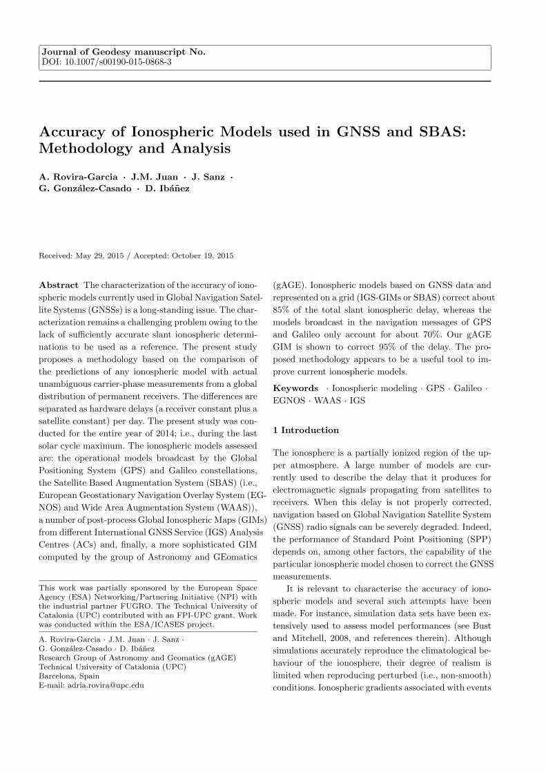
−120˚ −90˚ −60˚ −30˚ 0˚ 30˚ 60˚ 90˚ 120˚

−75˚

−60˚

−45˚

−30˚

−15˚

0˚

15˚

30˚

45˚

60˚

75˚

144 StationsGlobal Network:GIMs, NeQuick, Klobuchar

SBAS Networks:EGNOS Stations: 31WAAS Stations: 14

Fig. 1: Distribution of permanent receivers used to as-

sess ionospheric models for 2014. All stations are used

in the assessment of global models: GIMs, Klobuchar

GPS and NeQuick Galileo. The red and green subsets

of receivers are used to assess the real-time ionospheric

corrections of EGNOS and WAAS, respectively. Black

curves indicate 0° (solid), ±36° (dashes), ±60°(dash-

dots) MODIP latitudes.

used to compute the ionospheric models (Global Iono-

spheric Maps (GIMs) or Satellite Based Augmentation

System (SBAS)). Thus, the post-fit residuals represent

the minimum error associated with those models. A sec-

ond source of error in the ionospheric corrections occurs

in the interpolation from the stations that are used to

derive the ionospheric model to the user location. The

interpolation error increases in poorly sounded areas,

far from the stations used to derive each ionospheric

model (Rovira-Garcia et al, 2015), and under perturbed

ionospheric conditions that can be sampled by indica-

tors such as the geomagnetic indexDst or the Along Arc

TEC Rate (AATR) index, among other indicators (see

Datta-Barua et al, 2005; Sanz et al, 2014, respectively).

The actual, unambiguous, unbiased, undifferenced

carrier-phase measurements LI−BI, calculated for 2014

for the entire network of stations, can be downloaded

from the server www.gage.upc.edu/products. The avail-

ability of these reference values allows anyone to per-

form the proposed test, avoiding the complex data pro-

cessing required to obtain such unambiguous STECs,

explained earlier in this section.

3 Significance of the Methodology

Before assessing ionospheric models, we validate the

idea underlying our testing approach; i.e., how a ref-

erence ionospheric model consistently fits the unam-

biguous carrier-phase measurements plus two constant

parameters associated with the receiver and satellite

hardware delays in Eq. (3). To this end, two tests have

been conducted using code and carrier-phase measure-

ments, respectively.

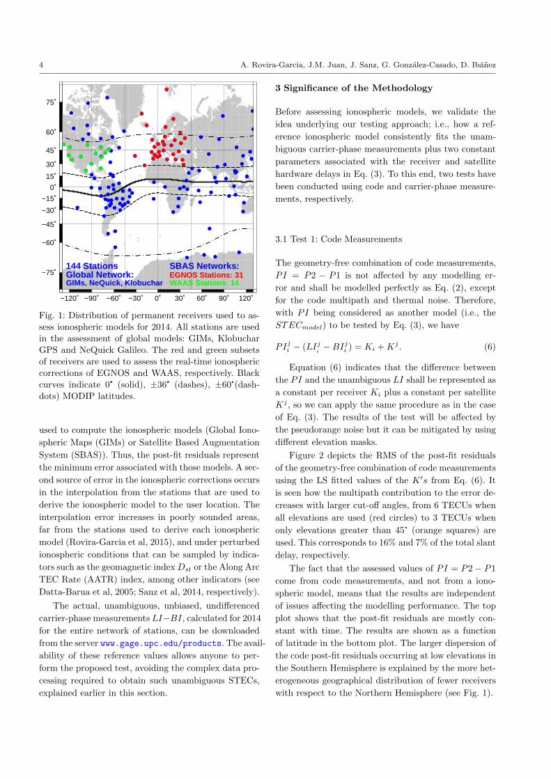
3.1 Test 1: Code Measurements

The geometry-free combination of code measurements,

PI = P2 − P1 is not affected by any modelling er-

ror and shall be modelled perfectly as Eq. (2), except

for the code multipath and thermal noise. Therefore,

with PI being considered as another model (i.e., the

STECmodel) to be tested by Eq. (3), we have

PIji − (LIji−BIji ) = Ki +Kj . (6)

Equation (6) indicates that the difference between

the PI and the unambiguous LI shall be represented as

a constant per receiver Ki plus a constant per satellite

Kj , so we can apply the same procedure as in the case

of Eq. (3). The results of the test will be affected by

the pseudorange noise but it can be mitigated by using

different elevation masks.

Figure 2 depicts the RMS of the post-fit residuals

of the geometry-free combination of code measurements

using the LS fitted values of the K ′s from Eq. (6). It

is seen how the multipath contribution to the error de-

creases with larger cut-off angles, from 6 TECUs when

all elevations are used (red circles) to 3 TECUs when

only elevations greater than 45° (orange squares) are

used. This corresponds to 16% and 7% of the total slant

delay, respectively.

The fact that the assessed values of PI = P2− P1

come from code measurements, and not from a iono-

spheric model, means that the results are independent

of issues affecting the modelling performance. The top

plot shows that the post-fit residuals are mostly con-

stant with time. The results are shown as a function

of latitude in the bottom plot. The larger dispersion of

the code post-fit residuals occurring at low elevations in

the Southern Hemisphere is explained by the more het-

erogeneous geographical distribution of fewer receivers

with respect to the Northern Hemisphere (see Fig. 1).

Accuracy of Ionospheric Models used in GNSS and SBAS: Methodology and Analysis 5

3.2 Test 2: Carrier-phase Measurements

The geometry-free combination of carrier-phase mea-

surements, LI, is an ionospheric measurement two or-

ders of magnitudes more precise than the code mea-

surements, but it is ambiguous. A widely used approach

taken to overcome the ambiguity is to align (level) such

carrier phases to the code measurements (e.g. Ciraolo

et al, 2007). The BI ambiguity is estimated as the mean

difference between the code and carrier phase per arc:

BIj

i ≈ 〈PIji − LI

ji 〉arc. (7)

As in the previous case, the test can be applied to

this geometry-free combination of carrier phases lev-

elled with the mean ambiguity, LI−BI. This is done by

replacing the PI by these code-levelled carrier phases

in Eq. (6) and estimating the corresponding K ′s of

Eq. (3).

The black crosses in Fig. 2 show the RMS of the

post-fit residuals of the test. In this code-levelling pro-

cedure, it is assumed that the thermal noise of the PI

is white noise with zero mean, being mostly removed in

the averaging operation of Eq. (7). The depicted RMS

of 1.5 TECU (4% of the total slant delay) then corre-

sponds to the residual multipath that produces an error

in the BI estimation. Note that no elevation or arc-

length constraint is applied. This result is of great in-

terest, since only code and carrier-phase measurements

are needed to generate such reference values, whereas

the computation of unambiguous STECs from carrier-

phase measurements with fixed ambiguities requires ac-

curate modelling and complex data processing, as ex-

plained in Section 2.

The code-levelled LI is used as the main input in

the determination of some ionospheric models. Note

that the multipath, responsible for 1.5 TECU of error,

is independent of the ionospheric activity. This error

can therefore be relevant in quiet ionospheric condi-

tions (e.g., conditions of the solar minimum or mid-

latitude regions). The final accuracy of the ionospheric

determinations is a function of the measurements used

(PI, code-levelled LI or ambiguity-fixed LI) and mod-

elling errors (e.g., geometric assumptions and temporal

or spatial interpolations), which will be analysed later

in Section 5 and 6.

4 Description of Ionospheric Models

After having introduced the methodology, it is worth

describing briefly the ionospheric models that were as-

0

1

2

3

4

5

6

7

8

9

10

Jan Feb Mar Apr May Jun Jul Aug Sep Oct Nov Dec Jan

RM

S P

ost-

fit R

esid

uals

(T

EC

Us)

Time (Month Of Year 2014)

PI Elevation > 05°PI Elevation > 15°PI Elevation > 30°PI Elevation > 45°

LI with BI = <PI-LI>

0

1

2

3

4

5

6

7

8

9

10

-70 -60 -50 -40 -30 -20 -10 0 10 20 30 40 50 60 70

RM

S P

ost-

fit R

esid

uals

(T

EC

Us)

Geographic Latitude (degrees)

PI Elevation > 05°PI Elevation > 15°PI Elevation > 30°PI Elevation > 45°

LI with BI = <PI-LI>

Fig. 2: Results of the consistency test for the geometry-

free combination of carrier-phase measurements (black)

and pseudoranges for different elevation cut-off angles:

5° (red), 15° (green), 30° (blue) and 45° (orange). The

horizontal axis gives the UT in the top plot and the

geographic latitude in the bottom plot.

sessed in this work. The characteristics of the iono-

spheric models used nowadays in GNSS have impor-

tant differences that determine the performances of the

models.

Klobuchar model. The Klobuchar model is a well-known

ionospheric model (Klobuchar, 1987) used by the GPS

and BeiDou Navigation Satellite System (BDS) (see IS-

GPS-200, 2010; China Satellite Navigation Office, 2012,

respectively). The model assumes that the ionospheric

delay occurs in a thin layer at a height of 350 km for the

GPS and 375 km for the BDS. The ionospheric predic-

tions are driven by a set of eight parameters broadcast

in the navigation message of each constellation and typ-

ically updated once per day.

NeQuick Galileo model. The original ionospheric model

(Di Giovanni and Radicella, 1990) has been adapted

6 A. Rovira-Garcia, J.M. Juan, J. Sanz, G. Gonzalez-Casado, D. Ibanez

for implementation in Galileo receivers (Prieto-Cerdeira

et al, 2014). The model is driven by a single parame-

ter (the effective ionisation level Az), which depends

on the MOdified DIP latitude (MODIP) (see Rawer,

1963) of the satellite Ionospheric Pierce Point (IPP) at

a height of 300 km. This dependency is modelled with a

second-order polynomial with three coefficients that are

broadcast in the Galileo navigation message (Galileo

SIS ICD, EU, 2010), and updated at least once a day.

International GNSS Service (IGS) GIMs. The IGS (see

Beutler et al, 1999; Dow et al, 2009) computes the

GIMs from actual GNSS observations collected by a

global network of permanent receivers. The Vertical To-

tal Electron Content (VTEC) is provided on a set of

Ionospheric Grid Points (IGPs) globally distributed in

a single layer at a height of 450 km, using a spatial

resolution of 2.5° in latitude and 5° in longitude. These

ionospheric grid maps are updated every 2 hours fol-

lowing the standard IONosphere map EXchange format

(IONEX) defined in Schaer et al (1998).

The IGS GIMs are computed by combining the de-

terminations from different Analysis Centres (ACs) into

the IGS Rapid and Final Products, available with 1 and

11 days of latency, respectively (International GNSS

Service Products, 2014). To demonstrate the perfor-

mance of shorter refreshing times, we assessed GIMs

from different ACs provided at a higher rate than the

standard 2-h IGS Rapid and Final Products. Indeed,

since 2013, European Space Operations Centre (ESOC)

and Centre for Orbit Determination in Europe (CODE)

have provided IONEX maps with a resolution of 1 hour

and Technical University of Catalonia (UPC) every 15

minutes (Dach and Jean, 2014).

SBAS ionospheric corrections. Geostationary satellites

broadcast to SBAS users the ionospheric model de-

scribed in the Minimum Operational Performance Standards

(MOPS) (RTCA, 2006). The model consists of VTEC

values on a single-layer grid at a height of 350 km. The

IGPs are spaced by 5° in both latitude and longitude,

increasing to 30° in longitude between 85° and the poles.

The maximum update time interval is 5 minutes.

The Fast Precise Point Positioning (Fast-PPP) iono-

spheric model. The group of Astronomy and GEomatics

(gAGE) has developed an ionospheric model with two

layers at heights of 270 and 1,600 km (Juan et al, 1997).

A forward, real-time estimation of the IGPs is made ev-

ery 5 minutes in regions where GNSS observations are

available. The model allows highly accurate navigation

with short convergence times, through what is known

as the Fast-PPP technique (Juan et al, 2012), and is

protected under the European Space Agency (ESA)

patent PCT/EP2011/001512 (2011).

The Fast-PPP ionospheric model maintains the lin-

ear distance between the IGPs in both the LT and the

MODIP axes. The distances are taken equal to 250 km

by 250 km for the bottom layer and to 500 km by

500 km for the top layer. Thus, the angular distance

between IGPs increases with the latitude, achieving

a constant resolution with a smaller number of IGPs

compared to the usual choice of using constant angular

steps. The use of two layers is particularly important

for precise navigation in low-latitude regions, as shown

in Rovira-Garcia et al (2015).

Fast-PPP GIMs. In the context of the project ICASES

(ESA, 2014), the Fast-PPP ionospheric model is smoothed

in post-processing to provide global coverage, since the

formal errors of the real-time model are large in poorly

sounded regions (e.g., oceans). The procedure includes

a backward estimation of the VTEC at the IGPs. All

regions are covered at a cost of partially degrading

the well-sounded IGPs, but still describing the vertical

description of the ionosphere (Garcıa-Fernandez et al,

2003). This smoothed dual-layer Fast-PPP GIM is up-

dated every 15 minutes and stored in LT and MODIP.

To ease its dissemination, it is also provided in a dual-

layer IONEX standard format (i.e., longitude and lat-

itude), which will be later referred to as gAGE GIM.

Although a standard, the latitude-based interpolation

has a resolution loss at low latitude with regard to the

MODIP-based interpolation (Azpilicueta et al, 2006).

Another important characteristic for such a GIM tai-

lored for GNSS is to provide realistic confidence bounds

to indicate where the VTEC is correctly determined.

5 Assessment of Global Ionospheric Models

The test described in Section 2 was routinely applied to

the set of receivers shown in Fig. 1 for 2014, which is a

year within the last solar cycle exhibiting the highest so-

lar activity. The software used to compute the different

model predictions was GNSS-Lab Tool suite (gLAB);

see Sanz et al (2012).

The daily mean of the RMS of the post-fit residuals

(i.e., the error) is plotted in Fig. 3 for the global iono-

spheric models described in Section 4, using two dif-

Accuracy of Ionospheric Models used in GNSS and SBAS: Methodology and Analysis 7

0

2

4

6

8

10

12

14

16

18

20

22

24

26

28

30

Jan Feb Mar Apr May Jun Jul Aug Sep Oct Nov Dec Jan

RM

S P

ost-

fit R

esid

uals

(T

EC

Us)

Time (Month Of Year 2014)

Mar

ch E

quin

ox

June

Sol

stic

e

Sep

tem

ber

Equ

inox

Dec

embe

r S

olst

ice

Klobuchar GPS ModelNeQuick GAL ModelIGS Rapid GIM (2 h)

gAGE GIM (15 min)Fast-PPP GIM (15 min)

Fast-PPP (5 min)

0

5

10

15

20

25

30

35

40

45

50

Jan Feb Mar Apr May Jun Jul Aug Sep Oct Nov Dec Jan

Rel

ativ

e R

MS

Pos

t-fit

Res

idua

ls w

rt U

nam

bigu

ous

LI (

%)

Time (Month Of Year 2014)

Klobuchar GPS ModelNeQuick GAL ModelIGS Rapid GIM (2 h)

gAGE GIM (15 min)Fast-PPP GIM (15 min)

Fast-PPP (5 min)

0

2

4

6

8

10

12

14

16

18

20

22

-70 -60 -50 -40 -30 -20 -10 0 10 20 30 40 50 60 70

RM

S P

ost-

fit R

esid

uals

(T

EC

Us)

Geographic Latitude (degrees)

Klobuchar GPS ModelNeQuick GAL ModelIGS Rapid GIM (2 h)

gAGE GIM (15 min)Fast-PPP GIM (15 min)

Fast-PPP (5 min)

0

5

10

15

20

25

30

35

40

45

50

-70 -60 -50 -40 -30 -20 -10 0 10 20 30 40 50 60 70

Rel

ativ

e R

MS

Pos

t-fit

Res

idua

ls w

rt U

nam

bigu

ous

LI (

%)

Geographic Latitude (degrees)

Klobuchar GPS ModelNeQuick GAL ModelIGS Rapid GIM (2 h)

gAGE GIM (15 min)Fast-PPP GIM (15 min)

Fast-PPP (5 min)

Fig. 3: Results of the consistency test among different global ionospheric models; Klobuchar (red) and NeQuick

Galileo (green) broadcast models, 2-h Rapid IGS GIM (dark blue), 15-min Fast-PPP GIM (light blue), the gAGE

GIM in the IONEX standard (orange), and the real-time (5-min) Fast-PPP model (black). The horizontal axis is

the universal time in the top row and latitude in the bottom row. The plots on the left present the absolute value

of the error and those on the right the relative value after dividing by the total slant delay.

ferent sets of axes; i.e., the UT in the top row and the

geographical latitude in the bottom row. The errors are

expressed in absolute terms (left column) and as per-

centages (right column) after dividing by the total slant

delay (i.e., the unambiguous LI). In this way, one can

derive the uncorrected portion of the total ionospheric

delay for each model.

The top row of Fig. 3 shows a seasonal structure

common to all analysed models. A ratio over 2 is ob-

served in Table 1 between the best and worst absolute

performances for each model, which occur around the

June solstice and March equinox, respectively. The rel-

ative variations are much smaller throughout the year,

suggesting that the correction capability of all iono-

spheric models is proportional to the global TEC.

The latitudinal examination of the test results clearly

reveals the different strategies used by the models. STECs

modelled with NeQuick Galileo (green) or Klobuchar

GPS (red) present errors around 8 TECUs in mid-latitude

regions and more than 20 TECUs at low latitudes. The

relative error is found to be more stable through the

year (see Table 1), being about 30% and 36% of the to-

tal slant delay for NeQuick Galileo and Klobuchar GPS

models, respectively.

Better STEC modelling is achieved using the post-

processed Rapid GIMs from IGS (dark blue), with er-

rors ranging from around 3 TECUs at mid-latitudes to

around 10 TECUs at equatorial latitudes. This corre-

sponds to an average modelling error of 16% of the to-

tal slant delay (see Table 1). Note that the test is done

over oblique STECs, and this result is thus better than

8 A. Rovira-Garcia, J.M. Juan, J. Sanz, G. Gonzalez-Casado, D. Ibanez

Table 1: Monthly results of the consistency test among different global ionospheric determinations. For each model,

values on the left column present the absolute error in TECUs (RMS) and those on the right the relative value

after dividing by the total slant delay.

MonthGPS Galileo

Fast-PPP Implementations IGS-GIMReal-Time MODIP GIM IONEX Rapid Product

RMS (%) RMS (%) RMS (%) RMS (%) RMS (%) RMS (%)January 14.60 42.17 11.71 33.80 0.18 0.52 1.75 5.05 2.19 6.32 5.92 17.10February 17.61 37.44 15.14 32.22 0.22 0.48 2.18 4.62 3.27 6.93 8.38 17.77

March 19.00 32.31 17.67 30.07 0.23 0.39 2.47 4.20 3.72 6.34 9.34 15.87April 17.53 34.77 15.15 30.66 0.21 0.41 2.15 4.26 3.30 6.57 8.17 16.20May 12.61 32.16 9.97 25.40 0.16 0.42 1.52 3.86 2.35 5.95 5.85 14.82June 9.35 29.75 8.78 28.17 0.16 0.51 1.10 3.46 1.43 4.54 4.23 13.38July 9.72 31.11 8.34 26.62 0.15 0.48 1.14 3.61 1.73 5.46 4.40 14.00

August 11.08 35.31 8.49 27.12 0.15 0.47 1.30 4.13 1.97 6.26 5.00 15.88September 14.54 35.55 11.10 27.16 0.20 0.48 1.95 4.79 2.95 7.22 7.21 17.61October 18.02 38.81 14.85 32.01 0.22 0.48 2.14 4.61 3.26 7.04 7.96 17.19

November 17.60 39.42 14.38 32.07 0.23 0.52 2.16 4.83 3.08 6.90 7.91 17.64December 16.56 41.97 13.66 34.65 0.23 0.58 2.08 5.28 2.83 7.17 7.59 19.26

Average 14.85 35.90 12.44 30.00 0.20 0.48 1.83 4.39 2.67 6.39 6.83 16.40

the IGS-GIM nominal accuracy of 2–8 TECUs for the

VTEC given in International GNSS Service Products

(2014).

The (MODIP-based) Fast-PPP GIMs show typical

error (light blue) in the STEC predictions of around

1 to 2 TECUs, which is maintained at low latitudes.

In mean, this corresponds to less than 5% modelling

error, according to Table 1. The gAGE GIMs show a

degradation of up to 4 TECUs (10% of the total slant

delay) at low latitudes, because the interpolation uses

the latitude (IONEX standard, orange) instead of the

MODIP. This is specially noticeable at the great spatial

gradients present in the equatorial ionosphere.

Finally, the Fast-PPP real-time estimates (black)

have the lowest error (less than 0.25 TECUs). The test

results reflect the losses occurring in the process of fit-

ting the STEC delays to vertical values at the IGPs of

the reference stations used to build the model. The use

of an adequate geometry (two layers, MODIP interpo-

lation), a short time update (5 min) and, remarkably,

the ambiguity fixing strategy allow to maintain the er-

ror under the 1% of the total slant delay at the reference

stations all year long (see Table 1).

5.1 High-rate GIMs

The ionosphere is a dynamic system driven by the Sun

photo-ionisation. The more frequently any ionospheric

model is updated, the better the model is expected

to reproduce the temporal variation of the ionospheric

delay throughout the day. To assess the effect of the

refresh rate, this subsection presents test results for

GIMs obtained from different IGS ACs using a higher

time resolution than the 2-hour update time of the IGS

Rapid and Final Products. ESOC and UPC GIMs are

tested starting on 19th October 2014, when CODE be-

gan providing IONEX maps once every hour.

Figure 4 depicts the test results of a number of GIMs

obtained from IGS and gAGE. The relative modelling

errors of the IGS Final (black) and Rapid (blue) Prod-

ucts are 16% and 18% of the total slant delay, respec-

tively. It can be observed that the IGS Final Product

provides an accuracy that is around 1 TECU better

than that of the IGS Rapid Product. Despite having

a double time resolution, a similar result is observed

comparing ESOC (1-h) GIM (pink) and the IGS Rapid

Product (2-h) modelling errors. However, the CODE

(1-h) GIMs (red) post-fit residuals are the 15% of the

total slant delay, which correspond to an improvement

by about 2 TECUs over the IGS Rapid Products.

The more frequent determinations every 15 min of

UPC GIMs (green) result in an error of 12% of the to-

tal slant delay, corresponding to an improvement of 3.5

TECUs over the IGS Rapid Products. Using the same

temporal resolution, but with an additional layer and

fixed ambiguities, gAGE GIMs (orange) improve the

modelling error to a 7% of the total slant delay, which

corresponds to an improvement by around 6 TECUs

over the IGS Rapid Products. The interpolation with

MODIP of the Fast-PPP GIMs (light blue) represents

an additional error reduction to the 5% of the total

slant delay, which corresponds to a 1.5 TECU improve-

ment regarding to latitude-based interpolation. It is

Accuracy of Ionospheric Models used in GNSS and SBAS: Methodology and Analysis 9

0

1

2

3

4

5

6

7

8

9

10

Nov Dec Jan

RM

S P

ost-

fit R

esid

uals

(T

EC

Us)

Time (Month Of Year 2014)

IGS Rapid GIM (2 h)IGS Final GIM (2 h)

CODE Final GIM (1 h)ESOC Rapid GIM (1 h)

UPC Rapid GIM (15 min)gAGE Rapid GIM (15 min)

Fast-PPP Rapid GIM (15 min)

Fig. 4: Results of the consistency test among different

global ionospheric models; 2-h IGS Rapid (blue) and

IGS Final (black) Combined Products, 1-h CODE (red)

and ESOC (pink), 15-min UPC (green), Fast-PPP GIM

in MODIP (light blue), the gAGE GIM in the IONEX

standard (orange). The horizontal axis gives the uni-

versal time.

concluded that ionospheric models are improved by in-

creasing the refresh frequency, but other factors (e.g.,

the receiver network, number of layers, and interpola-

tion coordinates) remain of great importance.

6 Assessment of Regional Ionospheric Models

The European Geostationary Navigation Overlay System

(EGNOS) and the Wide Area Augmentation System

(WAAS) provide ionospheric corrections within the re-

gions defined by European Civil Aviation Conference

(ECAC) (ECAC, 1955) and CONtiguous United States

(CONUS), respectively. For consistency, all the global

ionospheric models were validated over the same regions

(i.e., epochs, stations and satellites) for which the Euro-

pean and American SBASs provided ionospheric correc-

tions following the MOPS. Such IGS regional networks

of receivers are shown in Fig. 1 with red and green dots

for EGNOS and WAAS, respectively.

Figure 5 shows that, in Europe, the RMS of the

post-fit residuals of NeQuick Galileo (green) and Klobuchar

(red) models range from 6 to 20 TECUs; i.e., 20–45%

modelling error. It is noted that NeQuick Galileo most

outperforms Klobuchar at such European mid-latitudes.

The Rapid IGS GIMs (dark blue) present an RMS er-

ror of 3 to 12 TECUs, which corresponds to 8–25% of

the total ionospheric delay. The real-time EGNOS iono-

spheric corrections (pink) are at levels of 2 to 6 TECUs,

which corresponds to a 9% modelling error in average

(see Table 2). In this mid-latitude region with smaller

spatial gradients, there is no advantage in using the

Fast-PPP GIMs based on MODIP (light blue) with re-

spect to the gAGE GIMs based on latitude (orange).

In fact, at these latitudes, MODIP degrees are coarser

than geographic degrees. Both GIMs show errors at 1–

2 TECUs, which corresponds to a 5% modelling error.

Again, typical errors of the Fast-PPP model (black) are

well below 0.25 TECU.

Figure 6 shows equivalent results for North America.

All models improve by 1–2 TECUs with respect to the

European results, which corresponds to a modelling er-

ror of 3–5%. This is because the MODIP angular range

(which determines the challenges of the ionosphere) in

WAAS is 43–64 degrees while the EGNOS range is 35–

65 degrees (see Fig. 1). The RMS of the post-fit resid-

uals of the real-time ionospheric corrections of WAAS

(pink) are at the level of 2 TECUs, which corresponds

to a 6% modelling error (see Table 2). At first glance,

the WAAS accuracy seems to be better than the EG-

NOS accuracy, but when the two SBASs are compared

on the same MODIPs, the performance is almost iden-

tical. SBAS accuracies are slightly better than the IGS-

GIM probably owing to the higher refresh rate.

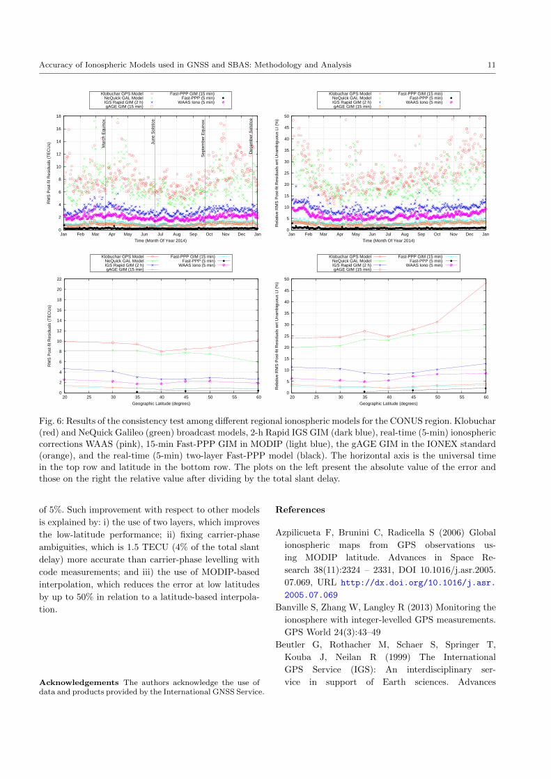
It becomes obvious that the Klobuchar GPS model

performs similarly to NeQuick Galileo in CONUS. More-

over, in ECAC area is where NeQuick Galileo remark-

ably improves the Klobuchar results. The accuracies of

both GPS and Galileo ionospheric models are better

over the WAAS and EGNOS areas than in the global

analysis of previous section, suggesting that the iono-

spheric coefficients of both constellations are optimised

for the particular regions CONUS and ECAC, respec-

tively.

7 Conclusions

A procedure was presented for the assessment of the

accuracy of ionospheric models for GNSS. The test is

based on actual, unambiguous, unbiased and undiffer-

enced carrier-phase measurements available at www.gage.

upc.edu/products. The strategy was routinely applied

for the entire year 2014, which is a year within the last

solar cycle exhibiting the highest solar activity.

On a global scale, it was shown that the errors of the

operational ionospheric models broadcast in real time

by GPS and Galileo constellations are about 35% of the

total slant delay. The NeQuick model for the Galileo

10 A. Rovira-Garcia, J.M. Juan, J. Sanz, G. Gonzalez-Casado, D. Ibanez

0

2

4

6

8

10

12

14

16

18

Jan Feb Mar Apr May Jun Jul Aug Sep Oct Nov Dec Jan

RM

S P

ost-

fit R

esid

uals

(T

EC

Us)

Time (Month Of Year 2014)

Mar

ch E

quin

ox

June

Sol

stic

e

Sep

tem

ber

Equ

inox

Dec

embe

r S

olst

ice

Klobuchar GPS ModelNeQuick GAL ModelIGS Rapid GIM (2 h)gAGE GIM (15 min)

Fast-PPP GIM (15 min)Fast-PPP (5 min)

EGNOS Iono (5 min)

0

5

10

15

20

25

30

35

40

45

50

Jan Feb Mar Apr May Jun Jul Aug Sep Oct Nov Dec Jan

Rel

ativ

e R

MS

Pos

t-fit

Res

idua

ls w

rt U

nam

bigu

ous

LI (

%)

Time (Month Of Year 2014)

Klobuchar GPS ModelNeQuick GAL ModelIGS Rapid GIM (2 h)gAGE GIM (15 min)

Fast-PPP GIM (15 min)Fast-PPP (5 min)

EGNOS Iono (5 min)

0

2

4

6

8

10

12

14

16

18

20

22

25 30 35 40 45 50 55 60 65

RM

S P

ost-

fit R

esid

uals

(T

EC

Us)

Geographic Latitude (degrees)

Klobuchar GPS ModelNeQuick GAL ModelIGS Rapid GIM (2 h)gAGE GIM (15 min)

Fast-PPP GIM (15 min)Fast-PPP (5 min)

EGNOS Iono (5 min)

0

5

10

15

20

25

30

35

40

45

50

25 30 35 40 45 50 55 60 65

Rel

ativ

e R

MS

Pos

t-fit

Res

idua

ls w

rt U

nam

bigu

ous

LI (

%)

Geographic Latitude (degrees)

Klobuchar GPS ModelNeQuick GAL ModelIGS Rapid GIM (2 h)gAGE GIM (15 min)

Fast-PPP GIM (15 min)Fast-PPP (5 min)

EGNOS Iono (5 min)

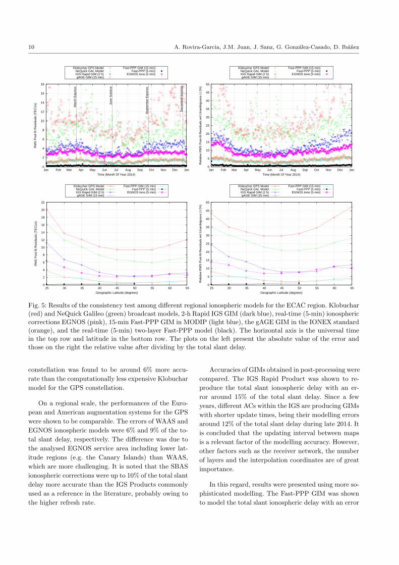
Fig. 5: Results of the consistency test among different regional ionospheric models for the ECAC region. Klobuchar

(red) and NeQuick Galileo (green) broadcast models, 2-h Rapid IGS GIM (dark blue), real-time (5-min) ionospheric

corrections EGNOS (pink), 15-min Fast-PPP GIM in MODIP (light blue), the gAGE GIM in the IONEX standard

(orange), and the real-time (5-min) two-layer Fast-PPP model (black). The horizontal axis is the universal time

in the top row and latitude in the bottom row. The plots on the left present the absolute value of the error and

those on the right the relative value after dividing by the total slant delay.

constellation was found to be around 6% more accu-

rate than the computationally less expensive Klobuchar

model for the GPS constellation.

On a regional scale, the performances of the Euro-

pean and American augmentation systems for the GPS

were shown to be comparable. The errors of WAAS and

EGNOS ionospheric models were 6% and 9% of the to-

tal slant delay, respectively. The difference was due to

the analysed EGNOS service area including lower lat-

itude regions (e.g. the Canary Islands) than WAAS,

which are more challenging. It is noted that the SBAS

ionospheric corrections were up to 10% of the total slant

delay more accurate than the IGS Products commonly

used as a reference in the literature, probably owing to

the higher refresh rate.

Accuracies of GIMs obtained in post-processing were

compared. The IGS Rapid Product was shown to re-

produce the total slant ionospheric delay with an er-

ror around 15% of the total slant delay. Since a few

years, different ACs within the IGS are producing GIMs

with shorter update times, being their modelling errors

around 12% of the total slant delay during late 2014. It

is concluded that the updating interval between maps

is a relevant factor of the modelling accuracy. However,

other factors such as the receiver network, the number

of layers and the interpolation coordinates are of great

importance.

In this regard, results were presented using more so-

phisticated modelling. The Fast-PPP GIM was shown

to model the total slant ionospheric delay with an error

Accuracy of Ionospheric Models used in GNSS and SBAS: Methodology and Analysis 11

0

2

4

6

8

10

12

14

16

18

Jan Feb Mar Apr May Jun Jul Aug Sep Oct Nov Dec Jan

RM

S P

ost-

fit R

esid

uals

(T

EC

Us)

Time (Month Of Year 2014)

Mar

ch E

quin

ox

June

Sol

stic

e

Sep

tem

ber

Equ

inox

Dec

embe

r S

olst

ice

Klobuchar GPS ModelNeQuick GAL ModelIGS Rapid GIM (2 h)gAGE GIM (15 min)

Fast-PPP GIM (15 min)Fast-PPP (5 min)

WAAS Iono (5 min)

0

5

10

15

20

25

30

35

40

45

50

Jan Feb Mar Apr May Jun Jul Aug Sep Oct Nov Dec Jan

Rel

ativ

e R

MS

Pos

t-fit

Res

idua

ls w

rt U

nam

bigu

ous

LI (

%)

Time (Month Of Year 2014)

Klobuchar GPS ModelNeQuick GAL ModelIGS Rapid GIM (2 h)gAGE GIM (15 min)

Fast-PPP GIM (15 min)Fast-PPP (5 min)

WAAS Iono (5 min)

0

2

4

6

8

10

12

14

16

18

20

22

20 25 30 35 40 45 50 55 60

RM

S P

ost-

fit R

esid

uals

(T

EC

Us)

Geographic Latitude (degrees)

Klobuchar GPS ModelNeQuick GAL ModelIGS Rapid GIM (2 h)gAGE GIM (15 min)

Fast-PPP GIM (15 min)Fast-PPP (5 min)

WAAS Iono (5 min)

0

5

10

15

20

25

30

35

40

45

50

20 25 30 35 40 45 50 55 60

Rel

ativ

e R

MS

Pos

t-fit

Res

idua

ls w

rt U

nam

bigu

ous

LI (

%)

Geographic Latitude (degrees)

Klobuchar GPS ModelNeQuick GAL ModelIGS Rapid GIM (2 h)gAGE GIM (15 min)

Fast-PPP GIM (15 min)Fast-PPP (5 min)

WAAS Iono (5 min)

Fig. 6: Results of the consistency test among different regional ionospheric models for the CONUS region. Klobuchar

(red) and NeQuick Galileo (green) broadcast models, 2-h Rapid IGS GIM (dark blue), real-time (5-min) ionospheric

corrections WAAS (pink), 15-min Fast-PPP GIM in MODIP (light blue), the gAGE GIM in the IONEX standard

(orange), and the real-time (5-min) two-layer Fast-PPP model (black). The horizontal axis is the universal time

in the top row and latitude in the bottom row. The plots on the left present the absolute value of the error and

those on the right the relative value after dividing by the total slant delay.

of 5%. Such improvement with respect to other models

is explained by: i) the use of two layers, which improves

the low-latitude performance; ii) fixing carrier-phase

ambiguities, which is 1.5 TECU (4% of the total slant

delay) more accurate than carrier-phase levelling with

code measurements; and iii) the use of MODIP-based

interpolation, which reduces the error at low latitudes

by up to 50% in relation to a latitude-based interpola-

tion.

Acknowledgements The authors acknowledge the use ofdata and products provided by the International GNSS Service.

References

Azpilicueta F, Brunini C, Radicella S (2006) Global

ionospheric maps from GPS observations us-

ing MODIP latitude. Advances in Space Re-

search 38(11):2324 – 2331, DOI 10.1016/j.asr.2005.

07.069, URL http://dx.doi.org/10.1016/j.asr.

2005.07.069

Banville S, Zhang W, Langley R (2013) Monitoring the

ionosphere with integer-levelled GPS measurements.

GPS World 24(3):43–49

Beutler G, Rothacher M, Schaer S, Springer T,

Kouba J, Neilan R (1999) The International

GPS Service (IGS): An interdisciplinary ser-

vice in support of Earth sciences. Advances

12 A. Rovira-Garcia, J.M. Juan, J. Sanz, G. Gonzalez-Casado, D. Ibanez

Table 2: Monthly results of the consistency test for the

WAAS (left) and EGNOS (right) ionospheric correc-

tions for CONUS and ECAC regions, respectively. For

each model, values on the left column present the abso-

lute error in TECUs (RMS) and those on the right the

relative value after dividing by the total slant delay.

MonthWAAS EGNOS

RMS (%) RMS (%)

January 1.92 9.18 2.86 14.01February 2.26 6.41 3.33 10.46

March 2.29 4.78 3.56 7.44April 2.29 5.54 3.11 7.42May 1.86 5.19 2.49 6.94June 1.67 5.33 2.36 7.22July 1.69 5.59 2.47 7.77

August 1.65 6.17 2.45 8.74September 1.85 5.91 2.98 9.41October 2.08 6.14 3.16 9.39

November 2.29 6.99 3.11 10.43December 2.30 7.89 3.03 12.15

Average 2.01 6.26 2.91 9.28

in Space Research 23(4):631–653, DOI 10.1016/

S0273-1177(99)00160-X, URL http://dx.doi.org/

10.1016/S0273-1177(99)00160-X

Bust GS, Mitchell CN (2008) History, current state, and

future directions of ionospheric imaging. Reviews of

Geophysics 46(1), DOI 10.1029/2006RG000212, URL

http://dx.doi.org/10.1029/2006RG000212

China Satellite Navigation Office (2012) BeiDou Nav-

igation Satellite System Signal in Space. Interface

Control Document

Ciraolo L, Azpilicueta F, Brunini C, Meza A, Radi-

cella S (2007) Calibration errors on experimental

slant total electron content (TEC) determined with

GPS. Journal of Geodesy 81(2):111–120, DOI 10.

1007/s00190-006-0093-1, URL http://dx.doi.org/

10.1007/s00190-006-0093-1

Collins P, Lahaye F, Heroux P, Bisnath S (2008)

Precise Point Positioning with Ambiguity Resolu-

tion using the Decoupled Clock Model. In: Proceed-

ings of the 21st International Technical Meeting of

the Satellite Division of The Institute of Navigation

(ION GNSS 2008), Savannah, GA, USA, pp 1315–

1322, URL https://www.ion.org/publications/

abstract.cfm?articleID=8043

Dach R, Jean Y (2014) IGS Technical Report 2013.

Tech. rep., Pasadena, USA

Datta-Barua S, Walter T, Altshuler E, Blanch J, Enge

P (2005) Dst as an Indicator of Potential Threats to

WAAS Integrity and Availability. In: Proceedings of

ION GPS 2005, USA, pp 2365–2373

Di Giovanni G, Radicella S (1990) An Analytical Model

of the Electron Density Profile in the Ionosphere.

Advances in Space Research 10(11):27–30, DOI 10.

1016/0273-1177(90)90301-F, URL http://dx.doi.

org/10.1016/0273-1177(90)90301-F

Dow J, Neilan RE, Rizos C (2009) The International

GNSS Service in a changing landscape of Global

Navigation Satellite Systems. Journal of Geodesy

83:191–198, DOI 10.1007/s00190-008-0300-3, URL

http://dx.doi.org/10.1007/s00190-008-0300-3

ECAC (1955) Constitution and Rules of Procedure of

the European Civil Aviation Conference (ECAC).

Paris, France

ESA (2014) ICASES: Ionospheric Conditions and As-

sociated Scenarios for EGNOS Selected from the last

Solar Cycle. PO1520026618/01.

Fu LL, Christensen EJ, Yamarone CA, Lefebvre

M, Menard Y, Dorrer M, Escudier P (1994)

TOPEX/POSEIDON mission overview. Journal of

Geophysical Research: Oceans 99(12):24,369–24,381,

DOI 10.1029/94JC01761, URL http://dx.doi.

org/10.1029/94JC01761

Galileo SIS ICD, EU (2010) Galileo Open Service

Signal In Space Control Document (OS SIS IDC),

Issue 1.1. URL http://ec.europa.eu/enterprise/

policies/satnav/galileo/open-service/index_

en.htm

Garcıa-Fernandez M, Hernandez-Pajares M, Juan JM,

Sanz J, Orus R, Coisson P, Nava B, Radicella

SM (2003) Combining ionosonde with ground GPS

data for electron density estimation. Journal of At-

mospheric and Solar-Terrestrial Physics 65:683–691,

DOI 10.1016/S1364-6826(03)00085-3, URL http://

adsabs.harvard.edu/abs/2003JASTP..65..683G

Ge M, Gendt M, Rothacher M, Shi C, Liu J (2008)

Resolution of GPS Carrier-Phase Ambiguities in Pre-

cise Point Positioning (PPP) with Daily Observa-

tions. Journal of Geodesy 82(7):389–399, DOI 10.

1007/s00190-007-0187-4, URL http://dx.doi.org/

10.1007/s00190-007-0187-4

Gonzalez-Casado G, Juan JM, Sanz J, Rovira-Garcia

A, Aragon-Angel A (2015) Ionospheric and plasmas-

pheric electron contents inferred from radio occulta-

tions and global ionospheric maps. Journal of Geo-

physical Research: Space Physics 120(7):5983–5997,

DOI 10.1002/2014JA020807, URL http://dx.doi.

org/10.1002/2014JA020807

Accuracy of Ionospheric Models used in GNSS and SBAS: Methodology and Analysis 13

Hernandez-Pajares M, Juan JM, Sanz J, Colombo

OL (2002) Improving the real-time ionospheric de-

termination from GPS sites at very long distances

over the equator. Journal of Geophysical Research:

Space Physics 107(A10):1296–1305, DOI 10.1029/

2001JA009203, URL http://dx.doi.org/10.1029/

2001JA009203

Imel DA (1994) Evaluation of the TOPEX/POSEIDON

dual-frequency ionosphere correction. Journal of

Geophysical Research: Oceans 99(C12):24,895–

24,906, DOI 10.1029/94JC01869, URL http:

//dx.doi.org/10.1029/94JC01869

International GNSS Service Products (2014) URL

http://www.igs.org/products/data

IS-GPS-200 (2010) GPS Interface Specification IS-

GPS-200. Revision E. URL http://www.gps.gov/

technical/icwg/IS-GPS-200E.pdf

Jee G, Lee HB, Kim YH, Chung JK, Cho J (2010) As-

sessment of GPS global ionosphere maps (GIM) by

comparison between CODE GIM and TOPEX/Jason

TEC data: Ionospheric perspective. Journal of Geo-

physical Research: Space Physics 115(A10), DOI

10.1029/2010JA015432, URL http://dx.doi.org/

10.1029/2010JA015432

Juan J, Rius A, Hernandez-Pajares M, Sanz J (1997)

A two-layer model of the ionosphere using Global

Positioning System data. Geophysical Research Let-

ters 24(4):393–396, DOI 10.1029/97GL00092, URL

http://dx.doi.org/10.1029/97GL00092

Juan J, Hernandez-Pajares M, Sanz J, Ramos-Bosch

P, Aragon-Angel A, Orus R, Ochieng W, Feng S,

Coutinho P, Samson J, Tossaint M (2012) Enhanced

Precise Point Positioning for GNSS Users. IEEE

Transactions on Geoscience and Remote Sensing

DOI 10.1109/TGRS.2012.2189888, URL http://dx.

doi.org/10.1109/TGRS.2012.2189888

Klobuchar J (1987) Ionospheric Time-Delay Algorithm

for Single-Frequency GPS Users. Aerospace and

Electronic Systems, IEEE Transactions on AES-

23(3):325–331, DOI 10.1109/TAES.1987.310829,

URL http://dx.doi.org/10.1109/TAES.1987.

310829

Lanyi GE, Roth T (1988) A comparison of mapped

and measured total ionospheric electron content us-

ing global positioning system and beacon satellite

observations. Radio Science 23(4):483–492, DOI 10.

1029/RS023i004p00483, URL http://dx.doi.org/

10.1029/RS023i004p00483

Laurichesse D, Mercier F (2007) Integer Ambi-

guity Resolution on Undifferenced GPS Phase

Measurements and Its Application to PPP. In:

Proceedings of the 20th International Technical

Meeting of the Satellite Division, Institute of

Navigation, Fort Worth, Texas (USA), pp 839

– 848, URL http://www.ion.org/publications/

abstract.cfm?articleID=7584

Lee HB, Jee G, Kim YH, Shim JS (2013) Characteris-

tics of global plasmaspheric TEC in comparison with

the ionosphere simultaneously observed by Jason-

1 satellite. Journal of Geophysical Research: Space

Physics 118(2):935–946, DOI 10.1002/jgra.50130,

URL http://dx.doi.org/10.1002/jgra.50130

Mannucci AJ, Wilson BD, Yuan DN, Ho CH, Lindqwis-

ter UJ, Runge TF (1998) A global mapping technique

for GPS-derived ionospheric total electron content

measurements. Radio Science 33(3):565–582, DOI

10.1029/97RS02707, URL http://dx.doi.org/10.

1029/97RS02707

Mervart L, Lukes Z, Rocken C, Iwabuchi T (2008) Pre-

cise Point Positioning with Ambiguity Resolution in

Real-Time. In: Proceedings of the 21st International

Technical Meeting of the Satellite Division of The In-

stitute of Navigation (ION GNSS 2008), Savannah,

GA, USA, pp 397–405, URL https://www.ion.org/

publications/abstract.cfm?articleID=7969

Misra P, Enge P (2001) Global Positioning System:

Signals, Measurements and Performance. Ganga-

Jamuna Press, Lincoln, MA, USA

Montenbruck O, Hauschild A, Steigenberger P (2014)

Differential Code Bias Estimation using Multi-GNSS

Observations and Global Ionosphere Maps. Nav-

igation 61(3):191–201, DOI 10.1002/navi.64, URL

http://dx.doi.org/10.1002/navi.64

Orus R, Hernandez-Pajares M, Juan J, Garcıa-

Fernandez M (2003) Validation of the GPS TEC

maps with TOPEX data. Advances in Space Re-

search 31(3):621–627, DOI http://dx.doi.org/10.

1016/S0273-1177(03)00026-7, URL http://dx.doi.

org/10.1016/S0273-1177(03)00026-7

PCT/EP2011/001512 (2011) Hernandez-Pajares, M.

and Juan, JM. and Sanz, J. and Samson, J. and Tos-

saint, M. Method, Apparatus and System for Deter-

mining a Position of an Object Having a Global Navi-

gation Satellite System Receiver by Processing Undif-

ferenced Data Like Carrier Phase Measurements and

External Products Like Ionosphere Data. (ESA ref:

ESA/PAT/566). URL https://patentscope.wipo.

14 A. Rovira-Garcia, J.M. Juan, J. Sanz, G. Gonzalez-Casado, D. Ibanez

int/search/en/WO2012130252

Prieto-Cerdeira R, Orus-Perez R, Breeuwer E,

Lucas-Rodriguez R, Falcone M (2014) The Eu-

ropean Way: Assessment of NeQuick Ionospheric

Model for Galileo Single-Frequency Users. GPS

World 25(6):53–58, URL http://gpsworld.com/

innovation-the-european-way

Rawer K (1963) Propagation of Decameter Waves (HF-

band) in Meteorological and Astronomical Influences

on Radio Wave Propagation. Ed. Landmark, B. Perg-

amon Press, New York

Rovira-Garcia A, Juan J, Sanz J, Gonzalez-Casado

G (2015) A Worldwide Ionospheric Model for

Fast Precise Point Positioning. Geoscience

and Remote Sensing, IEEE Transactions on

53(8):4596–4604, DOI 10.1109/TGRS.2015.2402598,

URL http://ieeexplore.ieee.org/xpl/

articleDetails.jsp?arnumber=7053952

RTCA (2006) Minimum Operational Performance

Standards for Global Positioning System/Wide Area

Augmentation System Airborne Equipment. RTCA

Document 229-C

Sanz J, Rovira-Garcia A, Hernandez-Pajares M

M; Juan, Ventura-Traveset J, Lopez-Echazarreta

C, Hein G (2012) The ESA/UPC GNSS-Lab Tool

(gLAB): An advanced educational and professional

package for GNSS data processing and analysis.

In: Proceedings of Toulouse Space Show 2012, 4th

International Conference on Space Applications,

Toulouse, France

Sanz J, Juan J, Hernandez-Pajares M (2013)

GNSS Data Processing, Vol. I: Fundamentals

and Algorithms. ESA Communications, ESTEC

TM-23/1, Noordwijk, the Netherlands, URL

http://www.navipedia.net/GNSS_Book/ESA_

GNSS-Book_TM-23_Vol_I.pdf

Sanz J, Juan J, Gonzalez-Casado G, Prieto-Cerdeira

R, S S, Orus R (2014) Novel Ionospheric Ac-

tivity Indicator Specifically Tailored for GNSS

Users. In: Proceedings of ION GNSS+ 2014,

Tampa, Florida (USA), pp 1173–1182, URL

http://www.ion.org/publications/abstract.

cfm?jp=p&articleID=12269

Schaer S, Gurtner W, Feltens J (1998) IONEX: The

IONosphere Map Exchange Format Version 1. In:

Proceeding of the IGS AC Workshop, Darmstadt,

Germany, pp 233–247, URL https://igscb.jpl.

nasa.gov/igscb/data/format/ionex1.pdf

Wubbena G (1988) GPS carrier phases and clock mod-

eling. In: Groten E, Strauss R (eds) GPS-Techniques

Applied to Geodesy and Surveying, Lecture Notes

in Earth Sciences, vol 19, Springer Berlin Heidel-

berg, pp 381–392, DOI 10.1007/BFb0011350, URL

http://dx.doi.org/10.1007/BFb0011350