Accumulation of driver and passenger mutations during ...antal/Mypapers/accum10.pdf · Accumulation...

Accumulation of driver and passengermutations during tumor progressionIvana Bozica,b, Tibor Antala,c, Hisashi Ohtsukid, Hannah Cartere, Dewey Kime, Sining Chenf, Rachel Karchine,Kenneth W. Kinzlerg, Bert Vogelsteing,1, and Martin A. Nowaka,b,h,1

aProgram for Evolutionary Dynamics, and bDepartment of Mathematics, Harvard University, Cambridge, MA 02138; cSchool of Mathematics, University ofEdinburgh, Edinburgh EH9-3JZ, United Kingdom; dDepartment of Value and Decision Science, Tokyo Institute of Technology, Tokyo 152-8552, Japan;eDepartment of Biomedical Engineering, Institute for Computational Medicine, Johns Hopkins University, Baltimore, MD 21218; fDepartment ofBiostatistics, School of Public Health, University of Medicine and Dentistry of New Jersey, Piscataway, NJ 08854; gLudwig Center for Cancer Genetics andTherapeutics, and Howard Hudges Medical Institute at Johns Hopkins Kimmel Cancer Center, Baltimore, MD 21231; and hDepartment of Organismic andEvolutionary Biology, Harvard University, Cambridge, MA 02138

Contributed by Bert Vogelstein, August 11, 2010 (sent for review May 26, 2010)

Major efforts to sequence cancer genomes are now occurringthroughout the world. Though the emerging data from thesestudies are illuminating, their reconciliation with epidemiologicand clinical observations poses a major challenge. In the currentstudy, we provide amathematical model that begins to address thischallenge. We model tumors as a discrete time branching processthat starts with a single driver mutation and proceeds as eachnew driver mutation leads to a slightly increased rate of clonalexpansion. Using the model, we observe tremendous variation inthe rate of tumor development—providing an understanding ofthe heterogeneity in tumor sizes and development times that havebeen observed by epidemiologists and clinicians. Furthermore, themodel provides a simple formula for the number of driver muta-tions as a function of the total number of mutations in the tumor.Finally, when applied to recent experimental data, the modelallows us to calculate the actual selective advantage provided bytypical somatic mutations in human tumors in situ. This selectiveadvantage is surprisingly small—0.004! 0.0004—and has majorimplications for experimental cancer research.

genetics ∣ mathematical biology

It is now well accepted that virtually all cancers result from theaccumulated mutations in genes that increase the fitness of a

tumor cell over that of the cells that surround it (1, 2). “Fitness”is defined as the net replication rate, i.e., the difference betweenthe rate of cell birth and cell death. As a result of advances intechnology and bioinformatics, it has recently become possibleto determine the entire compendium of mutant genes in a tumor(3–9). Studies to date have revealed a complex genome, with∼40–80 amino acid changing mutations present in a typical solidtumor (6–10). For low-frequency mutations, it is difficult to dis-tinguish “driver mutations”—defined as those that confer a selec-tive growth advantage to the cell—from “passenger mutations”(11–13). Passenger mutations are defined as those which donot alter fitness but occurred in a cell that coincidentally or sub-sequently acquired a driver mutation, and are therefore found inevery cell with that driver mutation. It is believed that only a smallfraction of the total mutations in a tumor are driver mutations,but new, quantitative models are clearly needed to help interpretthe significance of the mutational data and to put them into theperspective of modern clinical and experimental cancer research.

In most previous models of tumor evolution, mutations accu-mulate in cell populations of constant size (14–16) or of variablesize, but the models take into account only one or two mutations(17–21). Such models typically address certain (important) as-pects of cancer evolution, but not the whole process. Indeed,we now know that most solid tumors are the consequence ofmany sequential mutations, not just two. These tumors typicallycontain 40–100 coding gene alterations, including 5–15 drivermutations (6–9). The exploration of models with multiple muta-tions in growing tumor cell populations is therefore an essential

line of investigation which has just recently been initiated (22,23). In the model presented in this paper, we assume that eachnew driver mutation leads to a slightly faster tumor growth rate.This model is as simple as possible, because the analytical resultsdepend on only three parameters: the average driver mutationrate u, the average selective advantage associated with drivermutations s, and the average cell division time T.

Tumors are initiated by the first genetic alteration that pro-vides a relative fitness advantage. In the case of many leukemias,this would represent the first alteration of an oncogene, such as atranslocation between BCR (breakpoint cluster region gene) andABL (V-abl Abelson murine leukemia viral oncogene homolog 1gene). In the case of solid tumors, the mutation that initiated theprocess might actually be the second “hit” in a tumor suppressorgene—the first hit affects one allele, without causing a growthchange, whereas the second hit, in the opposite allele, leavesthe cell without any functional suppressor, in accord with thetwo-hit hypothesis (24). It is important to point out that weare modeling tumor progression, not initiation (14, 15), becauseprogression is rate limiting for cancer mortality—it generallyrequires three or more decades for metastatic cancers to developfrom initiated cells in humans.

Our first goal is to characterize the times at which successivedriver mutations arise in a tumor of growing size. We have em-ployed a discrete time branching process (25) for this purpose be-cause it makes the numerical simulations feasible. In a discretetime process, all cell divisions are synchronized. We presentanalytic formulas for this discrete time branching process andanalogous formulas for the continuous time case whenever possi-ble (SI Appendix). At each time step, a cell can either divide ordifferentiate, senesce, or die. In the context of tumor expansion,there is no difference between differentiation, death, and senes-cence, because none of these processes will result in a greater num-ber of tumor cells than present prior to that time step. We assumethat driver mutations reduce the probability that the cell will takethis second course, i.e., that it will differentiate, die, or senesce,henceforth grouped as “stagnate.” A cell with k driver mutationstherefore has a stagnation probability dk ¼ 1

2 ð1 − sÞk. The divisionprobability is bk ¼ 1 − dk. The parameter s characterizes theselective advantage provided by a driver mutation.

Author contributions: I.B., T.A., R.K., B.V., and M.A.N. designed research; I.B., T.A., H.O.,H.C., D.K., and S.C. performed research; I.B., T.A., H.O., H.C., D.K., S.C., R.K., and M.A.N.contributed new reagents/analytic tools; I.B., T.A., R.K., K.W.K., B.V., and M.A.N. analyzeddata; and I.B., T.A., R.K., K.W.K., B.V., and M.A.N. wrote the paper.

The authors declare no conflict of interest.

See Commentary on page 18241.1To whom correspondence may be addressed. E-mail: [email protected] [email protected].

This article contains supporting information online at www.pnas.org/lookup/suppl/doi:10.1073/pnas.1010978107/-/DCSupplemental.

www.pnas.org/cgi/doi/10.1073/pnas.1010978107 PNAS ∣ October 26, 2010 ∣ vol. 107 ∣ no. 43 ∣ 18545–18550

GEN

ETICS

APP

LIED

MAT

HEMAT

ICS

SEECO

MMEN

TARY

http://www.pnas.org/lookup/suppl/doi:10.1073/pnas.1010978107/-/DCSupplemental

http://www.pnas.org/lookup/suppl/doi:10.1073/pnas.1010978107/-/DCSupplemental/Appendix.pdf






When a cell divides, one of the daughter cells can receive anadditional driver mutation with probability u. The point mutationrate in tumors is estimated to be ∼5 × 10−10 per base pair per celldivision (26). We estimate that there are ∼34;000 positions in thegenome that could become driver mutations (see Materials andMethods and SI Appendix). As the rate of chromosome loss intumors is much higher than the rate of point mutation (14), asingle point mutation is rate limiting for inactivation of tumorsuppressor genes (when a point mutation in a tumor suppressorgene occurs, the other copy of that gene will likely be lost rela-tively quickly; ref. 27). The driver mutation rate is therefore∼3.4 × 10−5 per cell division (≈2 × 34;000 × 5 × 10−10), becauseu is the probability that one of the daughter cells will have anadditional mutation. Our theory can accommodate any realisticmutation rate and the major numerical results are only weaklyaffected by varying the mutation rate within a reasonable range.

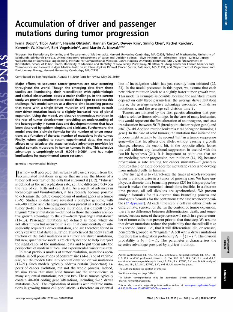
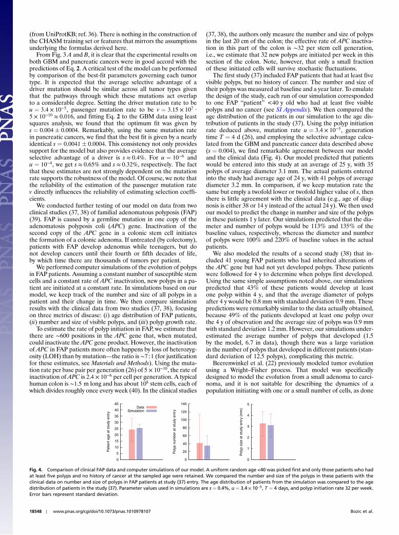
Experimental evidence suggests that tumor cells divide aboutonce every 3 d in glioblastoma multiforme (28) and once every 4 din colorectal cancers (26). Incorporating these division times intothe simulations provided by our model leads to the dramaticresults presented in Fig. 1. Though the same parameter values—u ¼ 3.4 × 10−5 and s ¼ 0.4%—were used for each simulation,there was enormous variation in the rates of disease progression.For example, in patient 1, the second driver mutation had onlyoccurred after 20 y following tumor initiation and the size ofthe tumor remained small (micrograms, representing <105 cells).

In contrast, in patient 6, the second driver mutation occurredafter less than 5 y, and by 25 y the tumor would weigh hundredsof grams (>1011 cells), with the most common cell type in thetumor having three driver mutations. Patients 2–5 had progres-sion rates between these two extreme cases.

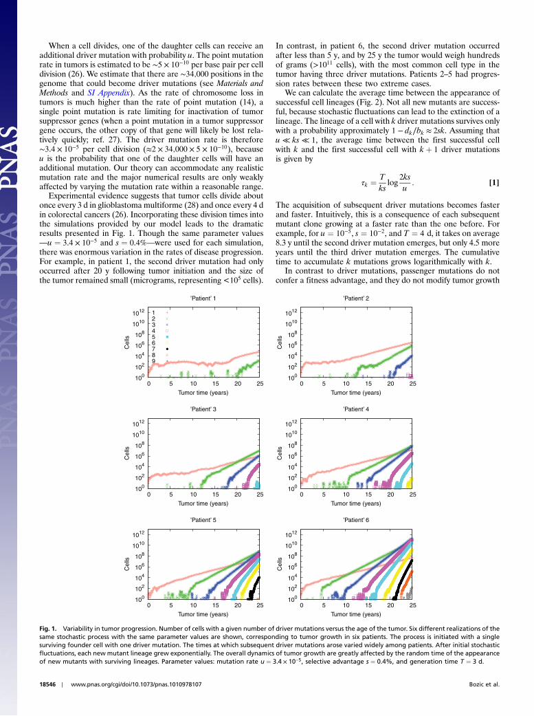
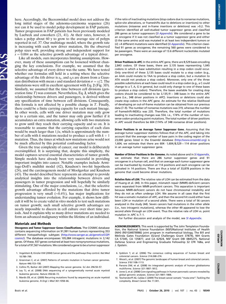
We can calculate the average time between the appearance ofsuccessful cell lineages (Fig. 2). Not all new mutants are success-ful, because stochastic fluctuations can lead to the extinction of alineage. The lineage of a cell with k driver mutations survives onlywith a probability approximately 1 − dk∕bk ≈ 2sk. Assuming thatu ≪ ks ≪ 1, the average time between the first successful cellwith k and the first successful cell with kþ 1 driver mutationsis given by

τk ¼Tks

log2ksu

: [1]

The acquisition of subsequent driver mutations becomes fasterand faster. Intuitively, this is a consequence of each subsequentmutant clone growing at a faster rate than the one before. Forexample, for u ¼ 10−5, s ¼ 10−2, and T ¼ 4 d, it takes on average8.3 y until the second driver mutation emerges, but only 4.5 moreyears until the third driver mutation emerges. The cumulativetime to accumulate k mutations grows logarithmically with k.

In contrast to driver mutations, passenger mutations do notconfer a fitness advantage, and they do not modify tumor growth

100

102

104

106

108

1010

1012

0 5 10 15 20 25

Cel

ls

Tumor time (years)

’Patient’ 1

123456789

100

102

104

106

108

1010

1012

0 5 10 15 20 25

Cel

ls

Tumor time (years)

’Patient’ 2

100

102

104

106

108

1010

1012

0 5 10 15 20 25

Cel

ls

Tumor time (years)

’Patient’ 3

100

102

104

106

108

1010

1012

0 5 10 15 20 25

Cel

ls

Tumor time (years)

’Patient’ 4

100

102

104

106

108

1010

1012

0 5 10 15 20 25

Cel

ls

Tumor time (years)

’Patient’ 5

100

102

104

106

108

1010

1012

0 5 10 15 20 25

Cel

ls

Tumor time (years)

’Patient’ 6

Fig. 1. Variability in tumor progression. Number of cells with a given number of driver mutations versus the age of the tumor. Six different realizations of thesame stochastic process with the same parameter values are shown, corresponding to tumor growth in six patients. The process is initiated with a singlesurviving founder cell with one driver mutation. The times at which subsequent driver mutations arose varied widely among patients. After initial stochasticfluctuations, each new mutant lineage grew exponentially. The overall dynamics of tumor growth are greatly affected by the random time of the appearanceof new mutants with surviving lineages. Parameter values: mutation rate u ¼ 3.4 × 10−5, selective advantage s ¼ 0.4%, and generation time T ¼ 3 d.

18546 ∣ www.pnas.org/cgi/doi/10.1073/pnas.1010978107 Bozic et al.


rates. We find that the average number of passenger mutations,nðtÞ, present in a tumor cell after t days is proportional to t, that isnðtÞ ¼ vt∕T, where v is the rate of acquisition of neutral muta-tions. In fact, v is the product of the point mutation rate per basepair and the number of base pairs analyzed. This simple relationhas been used to analyze experimental results by providing esti-mates for relevant time scales (26).

Combining our results for driver and passenger mutations,we can derive a formula for the number of passengers that areexpected in a tumor that has accumulated k driver mutations

n ¼ v2s

log4ks2

u2log k: [2]

Here, n is the number of passengers that were present in the lastcell that clonally expanded. Eq. 2 can be most easily applied totumors in tissues in which there is not much cell division prior to

tumor initiation. Otherwise, the expected number of passengersthat accumulated in a precursor cell prior to tumor initiationwould have to be included in the model, and this would be diffi-cult to estimate.

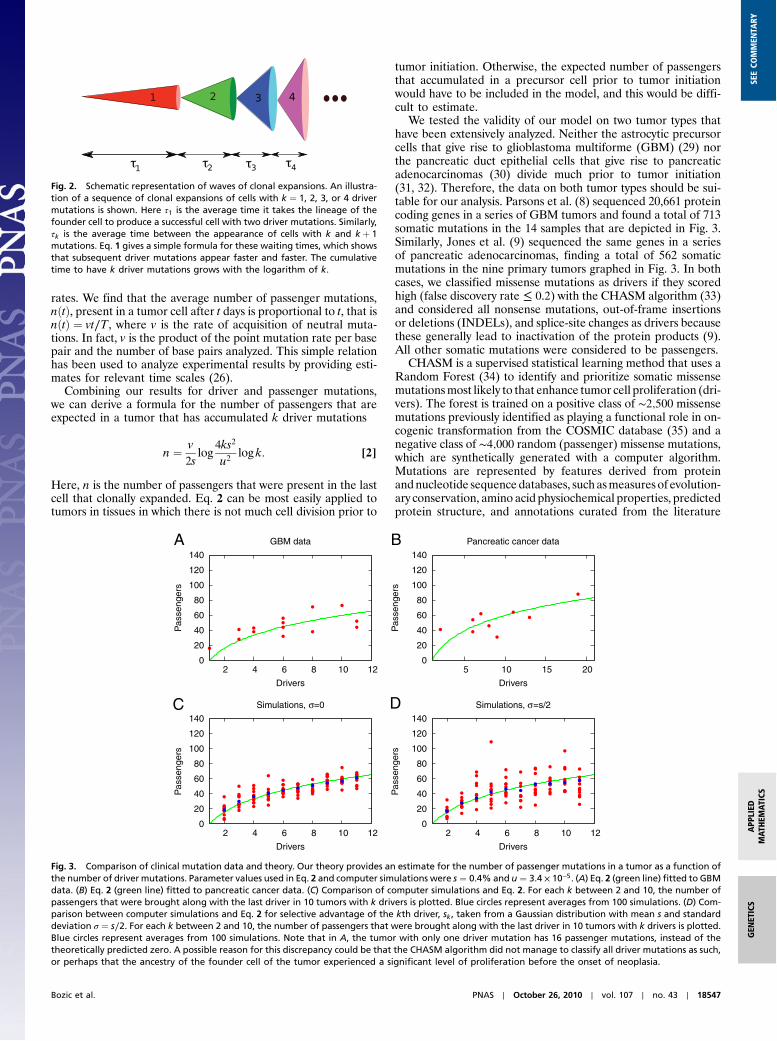
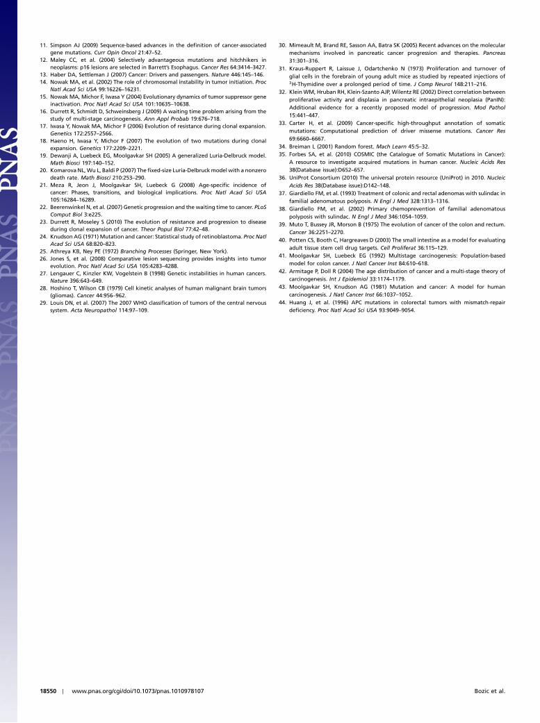
We tested the validity of our model on two tumor types thathave been extensively analyzed. Neither the astrocytic precursorcells that give rise to glioblastoma multiforme (GBM) (29) northe pancreatic duct epithelial cells that give rise to pancreaticadenocarcinomas (30) divide much prior to tumor initiation(31, 32). Therefore, the data on both tumor types should be sui-table for our analysis. Parsons et al. (8) sequenced 20,661 proteincoding genes in a series of GBM tumors and found a total of 713somatic mutations in the 14 samples that are depicted in Fig. 3.Similarly, Jones et al. (9) sequenced the same genes in a seriesof pancreatic adenocarcinomas, finding a total of 562 somaticmutations in the nine primary tumors graphed in Fig. 3. In bothcases, we classified missense mutations as drivers if they scoredhigh (false discovery rate ≤ 0.2) with the CHASM algorithm (33)and considered all nonsense mutations, out-of-frame insertionsor deletions (INDELs), and splice-site changes as drivers becausethese generally lead to inactivation of the protein products (9).All other somatic mutations were considered to be passengers.

CHASM is a supervised statistical learning method that uses aRandom Forest (34) to identify and prioritize somatic missensemutationsmost likely to that enhance tumor cell proliferation (dri-vers). The forest is trained on a positive class of ∼2;500 missensemutations previously identified as playing a functional role in on-cogenic transformation from the COSMIC database (35) and anegative class of ∼4;000 random (passenger) missense mutations,which are synthetically generated with a computer algorithm.Mutations are represented by features derived from proteinandnucleotide sequence databases, such asmeasures of evolution-ary conservation, amino acid physiochemical properties, predictedprotein structure, and annotations curated from the literature

Fig. 2. Schematic representation of waves of clonal expansions. An illustra-tion of a sequence of clonal expansions of cells with k ¼ 1, 2, 3, or 4 drivermutations is shown. Here τ1 is the average time it takes the lineage of thefounder cell to produce a successful cell with two driver mutations. Similarly,τk is the average time between the appearance of cells with k and k þ 1mutations. Eq. 1 gives a simple formula for these waiting times, which showsthat subsequent driver mutations appear faster and faster. The cumulativetime to have k driver mutations grows with the logarithm of k.

BA

0

20

40

60

80

100

120

140

2 4 6 8 10 12

Pas

seng

ers

Drivers

GBM data

0

20

40

60

80

100

120

140

5 10 15 20

Pas

seng

ers

Drivers

Pancreatic cancer data

DC

0

20

40

60

80

100

120

140

2 4 6 8 10 12

Pas

seng

ers

Drivers

Simulations, σ=0

0

20

40

60

80

100

120

140

2 4 6 8 10 12

Pas

seng

ers

Drivers

Simulations, σ=s/2

Fig. 3. Comparison of clinical mutation data and theory. Our theory provides an estimate for the number of passenger mutations in a tumor as a function ofthe number of driver mutations. Parameter values used in Eq. 2 and computer simulations were s ¼ 0.4% and u ¼ 3.4 × 10−5. (A) Eq. 2 (green line) fitted to GBMdata. (B) Eq. 2 (green line) fitted to pancreatic cancer data. (C) Comparison of computer simulations and Eq. 2. For each k between 2 and 10, the number ofpassengers that were brought along with the last driver in 10 tumors with k drivers is plotted. Blue circles represent averages from 100 simulations. (D) Com-parison between computer simulations and Eq. 2 for selective advantage of the kth driver, sk , taken from a Gaussian distribution with mean s and standarddeviation σ ¼ s∕2. For each k between 2 and 10, the number of passengers that were brought along with the last driver in 10 tumors with k drivers is plotted.Blue circles represent averages from 100 simulations. Note that in A, the tumor with only one driver mutation has 16 passenger mutations, instead of thetheoretically predicted zero. A possible reason for this discrepancy could be that the CHASM algorithm did not manage to classify all driver mutations as such,or perhaps that the ancestry of the founder cell of the tumor experienced a significant level of proliferation before the onset of neoplasia.

Bozic et al. PNAS ∣ October 26, 2010 ∣ vol. 107 ∣ no. 43 ∣ 18547

GEN

ETICS

APP

LIED

MAT

HEMAT

ICS

SEECO

MMEN

TARY

(fromUniProtKB; ref. 36). There is nothing in the construction ofthe CHASM training set or features that mirrors the assumptionsunderlying the formulas derived here.

From Fig. 3 A and B, it is clear that the experimental results onboth GBM and pancreatic cancers were in good accord with thepredictions of Eq. 2. A critical test of the model can be performedby comparison of the best-fit parameters governing each tumortype. It is expected that the average selective advantage of adriver mutation should be similar across all tumor types giventhat the pathways through which these mutations act overlapto a considerable degree. Setting the driver mutation rate to beu ¼ 3.4 × 10−5, passenger mutation rate to be v ¼ 3.15 × 107 ·5 × 10−10 ≈ 0.016, and fitting Eq. 2 to the GBM data using leastsquares analysis, we found that the optimum fit was given bys ¼ 0.004! 0.0004. Remarkably, using the same mutation ratein pancreatic cancers, we find that the best fit is given by a nearlyidentical s ¼ 0.0041! 0.0004. This consistency not only providessupport for the model but also provides evidence that the averageselective advantage of a driver is s ≈ 0.4%. For u ¼ 10−6 andu ¼ 10−4, we get s ≈ 0.65% and s ≈ 0.32%, respectively. The factthat these estimates are not strongly dependent on the mutationrate supports the robustness of the model. Of course, we note thatthe reliability of the estimation of the passenger mutation ratev directly influences the reliability of estimating selection coeffi-cients.

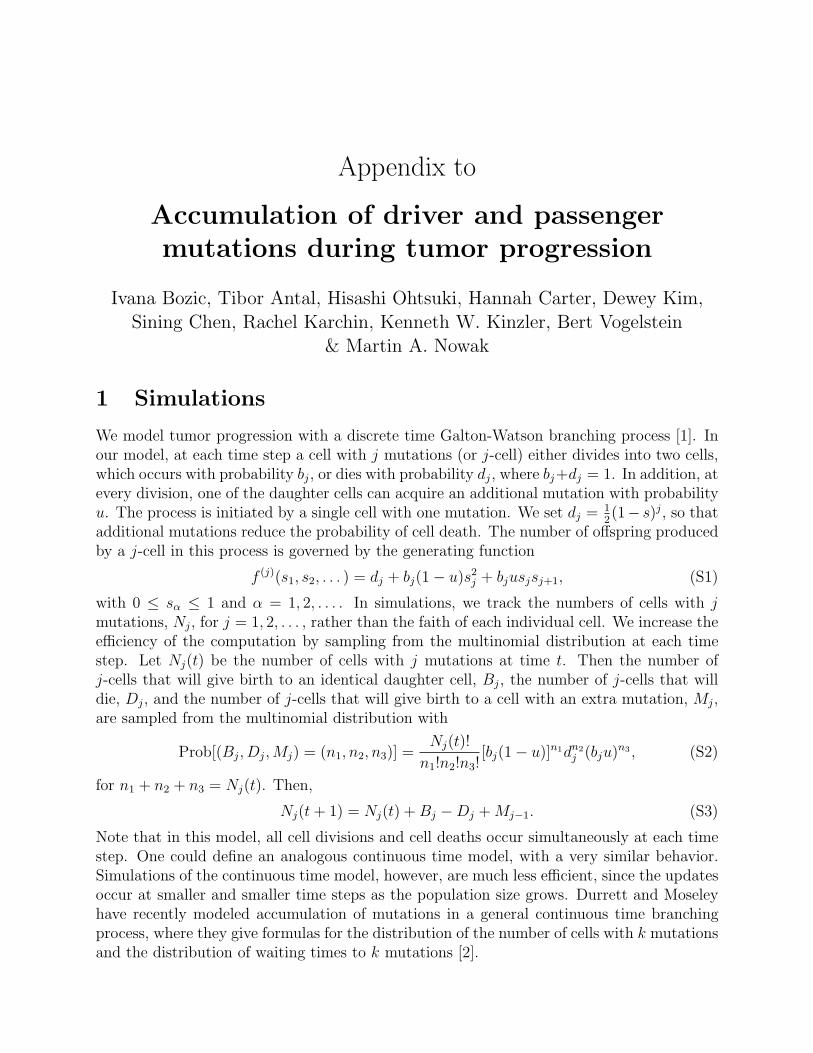
We conducted further testing of our model on data from twoclinical studies (37, 38) of familial adenomatous polyposis (FAP)(39). FAP is caused by a germline mutation in one copy of theadenomatosis polyposis coli (APC) gene. Inactivation of thesecond copy of the APC gene in a colonic stem cell initiatesthe formation of a colonic adenoma. If untreated (by colectomy),patients with FAP develop adenomas while teenagers, but donot develop cancers until their fourth or fifth decades of life,by which time there are thousands of tumors per patient.

We performed computer simulations of the evolution of polypsin FAP patients. Assuming a constant number of susceptible stemcells and a constant rate of APC inactivation, new polyps in a pa-tient are initiated at a constant rate. In simulations based on ourmodel, we keep track of the number and size of all polyps in apatient and their change in time. We then compare simulationresults with the clinical data from two studies (37, 38), focusingon three metrics of disease: (i) age distribution of FAP patients,(ii) number and size of visible polyps, and (iii) polyp growth rate.

To estimate the rate of polyp initiation in FAP, we estimate thatthere are ∼600 positions in the APC gene that, when mutated,could inactivate the APC gene product. However, the inactivationof APC in FAP patients more often happens by loss of heterozyg-osity (LOH) than by mutation—the ratio is ∼7∶1 (for justificationfor these estimates, see Materials and Methods). Using the muta-tion rate per base pair per generation (26) of 5 × 10−10, the rate ofinactivation of APC is 2.4 × 10−6 per cell per generation. A typicalhuman colon is ∼1.5 m long and has about 108 stem cells, each ofwhich divides roughly once every week (40). In the clinical studies

(37, 38), the authors only measure the number and size of polypsin the last 20 cm of the colon; the effective rate of APC inactiva-tion in this part of the colon is ∼32 per stem cell generation,i.e., we estimate that 32 new polyps are initiated per week in thissection of the colon. Note, however, that only a small fractionof these initiated cells will survive stochastic fluctuations.

The first study (37) included FAP patients that had at least fivevisible polyps, but no history of cancer. The number and size oftheir polyps was measured at baseline and a year later. To emulatethe design of the study, each run of our simulation correspondedto one FAP “patient” <40 y old who had at least five visiblepolyps and no cancer (see SI Appendix). We then compared theage distribution of the patients in our simulation to the age dis-tribution of patients in the study (37). Using the polyp initiationrate deduced above, mutation rate u ¼ 3.4 × 10−5, generationtime T ¼ 4 d (26), and employing the selective advantage calcu-lated from the GBM and pancreatic cancer data described above(s ¼ 0.004), we find remarkable agreement between our modeland the clinical data (Fig. 4). Our model predicted that patientswould be entered into this study at an average of 25 y, with 35polyps of average diameter 3.1 mm. The actual patients enteredinto the study had average age of 24 y, with 41 polyps of averagediameter 3.2 mm. In comparison, if we keep mutation rate thesame but emply a twofold lower or twofold higher value of s, thenthere is little agreement with the clinical data (e.g., age of diag-nosis is either 38 or 14 y instead of the actual 24 y). We then usedour model to predict the change in number and size of the polypsin these patients 1 y later. Our simulations predicted that the dia-meter and number of polyps would be 113% and 135% of thebaseline values, respectively, whereas the diameter and numberof polyps were 100% and 220% of baseline values in the actualpatients.

We also modeled the results of a second study (38) that in-cluded 41 young FAP patients who had inherited alterations ofthe APC gene but had not yet developed polyps. These patientswere followed for 4 y to determine when polyps first developed.Using the same simple assumptions noted above, our simulationspredicted that 43% of these patients would develop at leastone polyp within 4 y, and that the average diameter of polypsafter 4 y would be 0.8 mm with standard deviation 0.9 mm. Thesepredictions were remarkably similar to the data actually obtained,because 49% of the patients developed at least one polyp overthe 4 y of observation and the average size of polyps was 0.9 mmwith standard deviation 1.2 mm. However, our simulations under-estimated the average number of polyps that developed (1.5by the model, 6.7 in data), though there was a large variationin the number of polyps that developed in different patients (stan-dard deviation of 12.5 polyps), complicating this metric.

Beerenwinkel et al. (22) previously modeled tumor evolutionusing a Wright–Fisher process. That model was specificallydesigned to model the evolution from a small adenoma to carci-noma, and it is not suitable for describing the dynamics of apopulation initiating with one or a small number of cells, as done

0

5

10

15

20

25

30

35

40

45

Pat

ient

age

at s

tudy

ent

ry

DataSimulation

0

20

40

60

80

100

120

140

Pol

yp n

umbe

r at

stu

dy e

ntry

0

1

2

3

4

5

Pol

yp s

ize

at s

tudy

ent

ry (

mm

)

Fig. 4. Comparison of clinical FAP data and computer simulations of our model. A uniform random age <40was picked first and only those patients who hadat least five polyps and no history of cancer at the sampled age were retained. We compared the number and size of the polyps in these patients with theclinical data on number and size of polyps in FAP patients at study (37) entry. The age distribution of patients from the simulation was compared to the agedistribution of patients in the study (37). Parameter values used in simulations are s ¼ 0.4%, u ¼ 3.4 × 10−5, T ¼ 4 days, and polyp initiation rate 32 per week.Error bars represent standard deviation.



here. Accordingly, the Beerenwinkel model does not address thelong initial stages of the adenoma-carcinoma sequence (26)nor can it be used to model polyp development in FAP patients.Tumor progression in FAP patients has been previously modeledby Luebeck and coworkers (21, 41). At their rates, however, ittakes a polyp about 60 y to grow to the average size of polypsreported in ref. 37. Our multistage model, where the growth rateis increasing with each new driver mutation, fits the observedpolyp sizes well, providing strong and independent support fors ¼ 0.004 as the selective growth advantage of a typical driver.

Like all models, ours incorporates limiting assumptions. How-ever, many of these assumptions can be loosened without chan-ging the key conclusions. For example, we assumed that theselective advantage of every driver was the same. We have testedwhether our formulas still hold in a setting where the selectiveadvantage of the kth driver is sk, and sks are drawn from a Gaus-sian distribution with mean s and standard deviation σ ¼ s∕2. Thesimulations were still in excellent agreement with Eq. 2 (Fig. 3D).Similarly, we assumed that the time between cell divisions (gen-eration time T) was constant. Nevertheless, Eq. 2, which gives therelationship between drivers and passengers, is derived withoutany specification of time between cell divisions. Consequently,this formula is not affected by a possible change in T. Finally,there could be a finite carrying capacity for each mutant lineage.In other words, cells with one driver mutation may only growup to a certain size, and the tumor may only grow further if itaccumulates an extra mutation, allowing cells with two mutationsto grow until they reach their carrying capacity and so on. It isreasonable to assume that the carrying capacities of each classwould be much larger than 1∕u, which is approximately the num-ber of cells with k mutations needed to produce a cell with kþ 1mutation. Thus, the times at which newmutations arise would notbe much affected by this potential confounding factor.

Given the true complexity of cancer, our model is deliberatelyoversimplified. It is surprising that, despite this simplicity, themodel captures several essential characteristics of tumor growth.Simple models have already been very successful in providingimportant insights into cancer. Notable examples include Armi-tage-Doll’s multihit model (42), Knudson’s two-hit hypothesis(24), and the carcinogenesis model of Moolgavkar and Knudson(43). The model described here represents an attempt to provideanalytical insights into the relationship between drivers andpassengers in tumor progression and will hopefully be similarlystimulating. One of the major conclusions, i.e., that the selectivegrowth advantage afforded by the mutations that drive tumorprogression is very small (∼0.4%), has major implications forunderstanding tumor evolution. For example, it shows how diffi-cult it will be to create valid in vitro models to test such mutationson tumor growth; such small selective growth advantages arenearly impossible to discern in cell culture over short time per-iods. And it explains why so many driver mutations are needed toform an advanced malignancy within the lifetime of an individual.

Materials and MethodsOncogenes and Tumor Suppressor Genes Classifications. The COSMIC databasecontains sequencing information on 91,991 human tumors representing 353different histopathologic subtypes (http://www.sanger.ac.uk/genetics/CGP/cosmic/). The database encompasses 105,084 intragenic mutations in 3,142genes. Of these, 937 genes contained at least two nonsynynomousmutations,for a total of 97,567mutations.Weconsideredagene tobea tumor suppressor

if the ratio of inactivatingmutations (stop codons due to nonsensemutations,splice-site alterations, or frameshifts due to deletions or insertions) to othermutations (missense and in-frame insertions or deletions) was >0.2. Thiscriterion identified all well-studied tumor suppressor genes and classified286 genes as tumor suppressors (SI Appendix). We considered a gene to bean oncogene if it was not classified as a tumor suppressor gene and either(i) the same amino acid was mutated in at least two independent tumors or(ii) >4 different mutations were identified (SI Appendix). This criterion classi-fied 91 genes as oncogenes; the remaining 560 genes were considered tobe passengers. There were an average of 13.6 different nucleotides mutatedper oncogene.

Driver Positions in APC. In the entireAPC gene, there are 8,529 bases encoding2,843 codons. Of these bases, there are 3,135 bases representing 1,045codons in which a base substitution resulting in a stop codon could occur.Only one-third of these 3,135 bases could mutate to a stop codon (e.g.,an AAA could mutate to TAA to produce a stop codon, but a mutation toATA would not produce a stop codon). Moreover, only one of the threepossible substitutions at each base could result in a stop codon (e.g., a C couldchange to a T, A, G in general, but could only change to one of these basesto produce a stop codon). Therefore, the bases available for creating stopcodons should be considered to be 3;135∕9 ¼ 348 bases in the entire APCgene (i.e., 348 driver positions in APC). Insertions or deletions could alsocreate stop codons in the APC gene. An estimate for the relative likelihoodof developing an out-of-frame mutation can be obtained from our previousdata (7–9). The number of nonsense mutations was 319, whereas the numberof frameshift-INDELs was 235. Therefore, the total number of mutationsleading to inactivating changes was 554, i.e., 174% of the number of non-sense codon-producing point mutations. The total number of driver positionsin APC would therefore be 604 (174% of 348 nonsense driver positions).

Driver Positions in an Average Tumor Suppressor Gene. Assuming that theaverage tumor suppressor statistics follows that of the APC, and taking intoaccount that the average number of base pairs in the coding region of the23,000 genes listed in the Ensembl database (http://www.ensembl.org) is1,604, we estimate that there are 604 · 1;604∕8;529 ∼ 114 driver positionsin an average tumor suppressor gene.

Number of Driver Positions in the Genome. As noted above and in SI Appendix,we estimate that there are 286 tumor suppressor genes and 91oncogenes in a human cell, and that on average each tumor suppressor genecan be inactivated by mutation at 114 positions and each oncogene can beactivated in 14 positions. There are thus a total of 33,878 positions in thegenome that could become driver mutations.

Relative Rate of LOH. The relative rate of LOH can be estimated from the dataof Huang et al. (44). In this paper, mismatch repair (MMR)-deficient cancerswere separated from MMR-proficient cancers. This separation is importantbecause MMR-deficient cancers do not have chromosomal instability andthey do not as often undergo LOH. We assume in all cases that the firsthit was a somatic mutation of APC, and then the second hit could either havebeen LOH or mutation of a second allele. There were a total of 56 cancersanalyzed in the study (44). Seven cancers had mutations in the other allele(i.e., two intragenic mutations), whereas the other 49 appeared to lose thesecond allele through an LOH event. Thus the relative rate of LOH vs. pointmutation in APC is 7∶1.

For further discussion and analysis of the model, see SI Appendix.

ACKNOWLEDGMENTS. This work is supported by The John Templeton Founda-tion, the National Science Foundation (NSF)/National Institutes of Health(NIH) (R01GM078986) joint program in mathematical biology, The Bill andMelinda Gates Foundation (Grand Challenges Grant 37874), NIH GrantsCA 57345, CA 135877, and CA 62924, NSF Grant DBI 0845275, NationalDefense Science and Engineering Graduate Fellowship 32 CFR 168a, andJ. Epstein.

1. Vogelstein B, Kinzler KW (2004) Cancer genes and the pathways they control. NatMed10:789–799.

2. Greenman C, et al. (2007) Patterns of somatic mutation in human cancer genomes.Nature 446:153–158.

3. Collins FS, Barker AD (2007) Mapping the cancer genome. Sci Am 296:50–57.4. Ley TJ, et al. (2008) DNA sequencing of a cytogenetically normal acute myeloid

leukemia genome. Nature 456:66–72.5. Mardis ER, et al. (2009) Recurring mutations found by sequencing an acute myeloid

leukemia genome. N Engl J Med 361:1058–66.

6. Sjoblom T, et al. (2006) The consensus coding sequences of human breast andcolorectal cancers. Science 314:268–274.

7. Wood L, et al. (2007) The genomic landscapes of human breast and colorectal cancers.Science 318:1108–1113.

8. Parsons DW, et al. (2008) An integrated genomic analysis of human glioblastomamultiforme. Science 321:1807–1812.

9. Jones S, et al. (2008) Core signaling pathways in human pancreatic cancers revealed byglobal genomic analyses. Science 321:1801–1806.

10. Teschendorff AE, Caldas C (2009) The breast cancer somatic “muta-ome”: Tackling thecomplexity. Breast Cancer Res 11:301.

Bozic et al. PNAS ∣ October 26, 2010 ∣ vol. 107 ∣ no. 43 ∣ 18549

GEN

ETICS

APP

LIED

MAT

HEMAT

ICS

SEECO

MMEN

TARY


http://www.sanger.ac.uk/genetics/CGP/cosmic/







http://www.ensembl.org




11. Simpson AJ (2009) Sequence-based advances in the definition of cancer-associatedgene mutations. Curr Opin Oncol 21:47–52.

12. Maley CC, et al. (2004) Selectively advantageous mutations and hitchhikers inneoplasms: p16 lesions are selected in Barrett’s Esophagus. Cancer Res 64:3414–3427.

13. Haber DA, Settleman J (2007) Cancer: Drivers and passengers. Nature 446:145–146.14. Nowak MA, et al. (2002) The role of chromosomal instability in tumor initiation. Proc

Natl Acad Sci USA 99:16226–16231.15. Nowak MA, Michor F, Iwasa Y (2004) Evolutionary dynamics of tumor suppressor gene

inactivation. Proc Natl Acad Sci USA 101:10635–10638.16. Durrett R, Schmidt D, Schweinsberg J (2009) A waiting time problem arising from the

study of multi-stage carcinogenesis. Ann Appl Probab 19:676–718.17. Iwasa Y, Nowak MA, Michor F (2006) Evolution of resistance during clonal expansion.

Genetics 172:2557–2566.18. Haeno H, Iwasa Y, Michor F (2007) The evolution of two mutations during clonal

expansion. Genetics 177:2209–2221.19. Dewanji A, Luebeck EG, Moolgavkar SH (2005) A generalized Luria-Delbruck model.

Math Biosci 197:140–152.20. Komarova NL,Wu L, Baldi P (2007) The fixed-size Luria-Delbruckmodel with a nonzero

death rate. Math Biosci 210:253–290.21. Meza R, Jeon J, Moolgavkar SH, Luebeck G (2008) Age-specific incidence of

cancer: Phases, transitions, and biological implications. Proc Natl Acad Sci USA105:16284–16289.

22. Beerenwinkel N, et al. (2007) Genetic progression and the waiting time to cancer. PLoSComput Biol 3:e225.

23. Durrett R, Moseley S (2010) The evolution of resistance and progression to diseaseduring clonal expansion of cancer. Theor Popul Biol 77:42–48.

24. Knudson AG (1971) Mutation and cancer: Statistical study of retinoblastoma. Proc NatlAcad Sci USA 68:820–823.

25. Athreya KB, Ney PE (1972) Branching Processes (Springer, New York).26. Jones S, et al. (2008) Comparative lesion sequencing provides insights into tumor

evolution. Proc Natl Acad Sci USA 105:4283–4288.27. Lengauer C, Kinzler KW, Vogelstein B (1998) Genetic instabilities in human cancers.

Nature 396:643–649.28. Hoshino T, Wilson CB (1979) Cell kinetic analyses of human malignant brain tumors

(gliomas). Cancer 44:956–962.29. Louis DN, et al. (2007) The 2007 WHO classification of tumors of the central nervous

system. Acta Neuropathol 114:97–109.

30. Mimeault M, Brand RE, Sasson AA, Batra SK (2005) Recent advances on the molecularmechanisms involved in pancreatic cancer progression and therapies. Pancreas31:301–316.

31. Kraus-Ruppert R, Laissue J, Odartchenko N (1973) Proliferation and turnover ofglial cells in the forebrain of young adult mice as studied by repeated injections of3H-Thymidine over a prolonged period of time. J Comp Neurol 148:211–216.

32. KleinWM, Hruban RH, Klein-Szanto AJP, Wilentz RE (2002) Direct correlation betweenproliferative activity and displasia in pancreatic intraepithelial neoplasia (PanIN):Additional evidence for a recently proposed model of progression. Mod Pathol15:441–447.

33. Carter H, et al. (2009) Cancer-specific high-throughput annotation of somaticmutations: Computational prediction of driver missense mutations. Cancer Res69:6660–6667.

34. Breiman L (2001) Random forest. Mach Learn 45:5–32.35. Forbes SA, et al. (2010) COSMIC (the Catalogue of Somatic Mutations in Cancer):

A resource to investigate acquired mutations in human cancer. Nucleic Acids Res38(Database issue):D652–657.

36. UniProt Consortium (2010) The universal protein resource (UniProt) in 2010. NucleicAcids Res 38(Database issue):D142–148.

37. Giardiello FM, et al. (1993) Treatment of colonic and rectal adenomas with sulindac infamilial adenomatous polyposis. N Engl J Med 328:1313–1316.

38. Giardiello FM, et al. (2002) Primary chemoprevention of familial adenomatouspolyposis with sulindac. N Engl J Med 346:1054–1059.

39. Muto T, Bussey JR, Morson B (1975) The evolution of cancer of the colon and rectum.Cancer 36:2251–2270.

40. Potten CS, Booth C, Hargreaves D (2003) The small intestine as a model for evaluatingadult tissue stem cell drug targets. Cell Proliferat 36:115–129.

41. Moolgavkar SH, Luebeck EG (1992) Multistage carcinogenesis: Population-basedmodel for colon cancer. J Natl Cancer Inst 84:610–618.

42. Armitage P, Doll R (2004) The age distribution of cancer and a multi-stage theory ofcarcinogenesis. Int J Epidemiol 33:1174–1179.

43. Moolgavkar SH, Knudson AG (1981) Mutation and cancer: A model for humancarcinogenesis. J Natl Cancer Inst 66:1037–1052.

44. Huang J, et al. (1996) APC mutations in colorectal tumors with mismatch-repairdeficiency. Proc Natl Acad Sci USA 93:9049–9054.


Appendix to

Accumulation of driver and passengermutations during tumor progression

Ivana Bozic, Tibor Antal, Hisashi Ohtsuki, Hannah Carter, Dewey Kim,Sining Chen, Rachel Karchin, Kenneth W. Kinzler, Bert Vogelstein

& Martin A. Nowak

1 Simulations

We model tumor progression with a discrete time Galton-Watson branching process [1]. Inour model, at each time step a cell with j mutations (or j-cell) either divides into two cells,which occurs with probability bj, or dies with probability dj, where bj+dj = 1. In addition, atevery division, one of the daughter cells can acquire an additional mutation with probabilityu. The process is initiated by a single cell with one mutation. We set dj = 1

2(1� s)j, so thatadditional mutations reduce the probability of cell death. The number of o�spring producedby a j-cell in this process is governed by the generating function

f (j)(s1, s2, . . . ) = dj + bj(1� u)s2j + bjusjsj+1, (S1)

with 0 ⇥ s� ⇥ 1 and � = 1, 2, . . . . In simulations, we track the numbers of cells with jmutations, Nj, for j = 1, 2, . . . , rather than the faith of each individual cell. We increase thee⇥ciency of the computation by sampling from the multinomial distribution at each timestep. Let Nj(t) be the number of cells with j mutations at time t. Then the number ofj-cells that will give birth to an identical daughter cell, Bj, the number of j-cells that willdie, Dj, and the number of j-cells that will give birth to a cell with an extra mutation, Mj,are sampled from the multinomial distribution with

Prob[(Bj, Dj, Mj) = (n1, n2, n3)] =Nj(t)!

n1!n2!n3![bj(1� u)]n1dn2

j (bju)n3 , (S2)

for n1 + n2 + n3 = Nj(t). Then,

Nj(t + 1) = Nj(t) + Bj �Dj + Mj�1. (S3)

Note that in this model, all cell divisions and cell deaths occur simultaneously at each timestep. One could define an analogous continuous time model, with a very similar behavior.Simulations of the continuous time model, however, are much less e⇥cient, since the updatesoccur at smaller and smaller time steps as the population size grows. Durrett and Moseleyhave recently modeled accumulation of mutations in a general continuous time branchingprocess, where they give formulas for the distribution of the number of cells with k mutationsand the distribution of waiting times to k mutations [2].

0

2

4

6

8

10

12

14

16

1 2 3 4 5 6 7 8 9 10

! j (

ye

ars

)

j

s=0.005s=0.01s=0.02

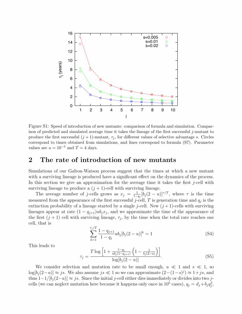
Figure S1: Speed of introduction of new mutants: comparison of formula and simulation. Compar-ison of predicted and simulated average time it takes the lineage of the first successful j-mutant toproduce the first successful (j + 1)-mutant, �j , for di�erent values of selective advantage s. Circlescorrespond to times obtained from simulations, and lines correspond to formula (S7). Parametervalues are u = 10�5 and T = 4 days.

2 The rate of introduction of new mutants

Simulations of our Galton-Watson process suggest that the times at which a new mutantwith a surviving lineage is produced have a significant e�ect on the dynamics of the process.In this section we give an approximation for the average time it takes the first j-cell withsurviving lineage to produce a (j + 1)-cell with surviving lineage.

The average number of j-cells grows as xj = 11�qj

[bj(2 � u)]�/T , where � is the timemeasured from the appearance of the first successful j-cell, T is generation time and qj is theextinction probability of a lineage started by a single j-cell. New (j +1)-cells with survivinglineages appear at rate (1 � qj+1)ubjxj, and we approximate the time of the appearance ofthe first (j + 1) cell with surviving lineage, �j, by the time when the total rate reaches onecell, that is

�j/T⇤

k=1

1� qj+1

1� qjubj[bj(2� u)]k = 1 (S4)

This leads to

�j =T log

⌅1 + 1�qj

ubj(1�qj+1)

�1� 1

bj(2�u)

⇥⇧

log[bj(2� u)]. (S5)

We consider selection and mutation rate to be small enough, u ⇤ 1 and s ⇤ 1, solog[bj(2�u)] ⇥ js. We also assume js⇤ 1 so we can approximate (2�(1�s)j) ⇥ 1+js, andthus 1�1/[bj(2�u)] ⇥ js. Since the initial j-cell either dies immediately or divides into two j-cells (we can neglect mutation here because it happens only once in 105 cases), qj = dj +bjq2

j ,

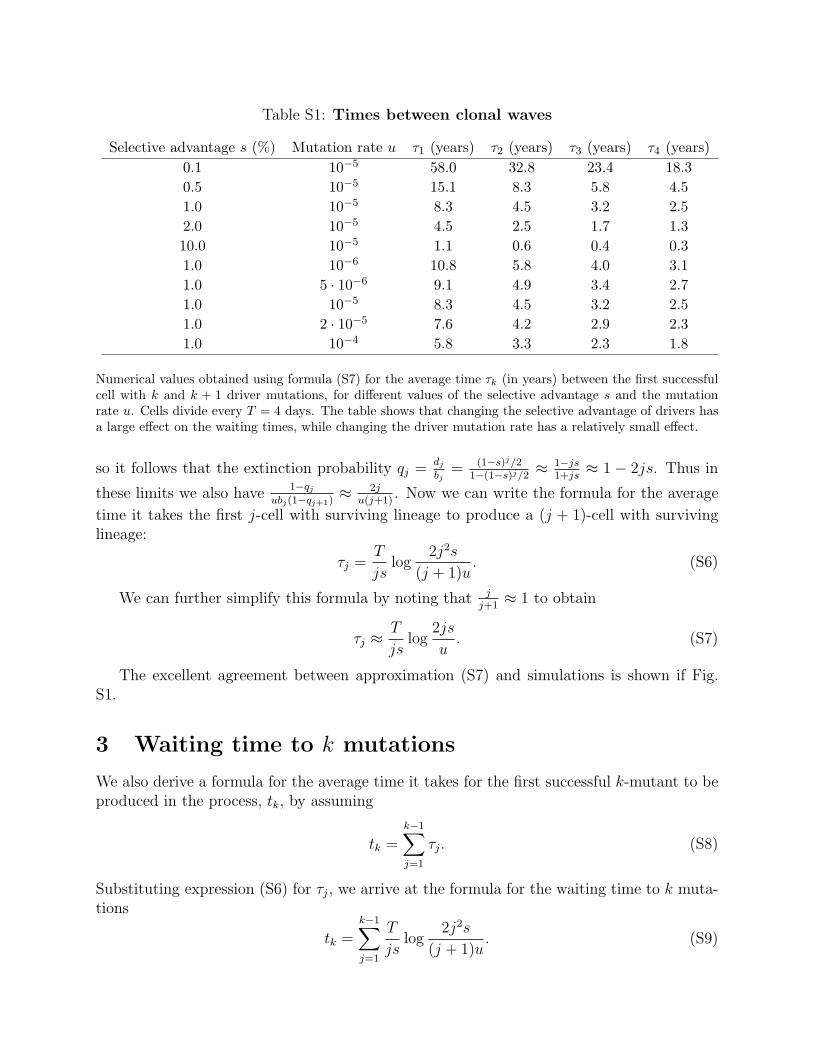
Table S1: Times between clonal waves

Selective advantage s (%) Mutation rate u �1 (years) �2 (years) �3 (years) �4 (years)0.1 10�5 58.0 32.8 23.4 18.30.5 10�5 15.1 8.3 5.8 4.51.0 10�5 8.3 4.5 3.2 2.52.0 10�5 4.5 2.5 1.7 1.310.0 10�5 1.1 0.6 0.4 0.31.0 10�6 10.8 5.8 4.0 3.11.0 5 · 10�6 9.1 4.9 3.4 2.71.0 10�5 8.3 4.5 3.2 2.51.0 2 · 10�5 7.6 4.2 2.9 2.31.0 10�4 5.8 3.3 2.3 1.8

Numerical values obtained using formula (S7) for the average time �k (in years) between the first successfulcell with k and k + 1 driver mutations, for di�erent values of the selective advantage s and the mutationrate u. Cells divide every T = 4 days. The table shows that changing the selective advantage of drivers hasa large e�ect on the waiting times, while changing the driver mutation rate has a relatively small e�ect.

so it follows that the extinction probability qj = dj

bj= (1�s)j/2

1�(1�s)j/2 ⇥1�js1+js ⇥ 1 � 2js. Thus in

these limits we also have 1�qj

ubj(1�qj+1) ⇥2j

u(j+1) . Now we can write the formula for the average

time it takes the first j-cell with surviving lineage to produce a (j + 1)-cell with survivinglineage:

�j =T

jslog

2j2s

(j + 1)u. (S6)

We can further simplify this formula by noting that jj+1 ⇥ 1 to obtain

�j ⇥T

jslog

2js

u. (S7)

The excellent agreement between approximation (S7) and simulations is shown if Fig.S1.

3 Waiting time to k mutations

We also derive a formula for the average time it takes for the first successful k-mutant to beproduced in the process, tk, by assuming

tk =k�1�

j=1

�j. (S8)

Substituting expression (S6) for �j, we arrive at the formula for the waiting time to k muta-tions

tk =k�1�

j=1

T

jslog

2j2s

(j + 1)u. (S9)

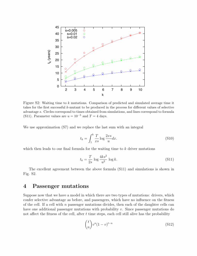
0

5

10

15

20

25

30

35

40

45

2 3 4 5 6 7 8 9 10

t k (

ye

ars

)

k

s=0.005s=0.01s=0.02

Figure S2: Waiting time to k mutations. Comparison of predicted and simulated average time ittakes for the first successful k-mutant to be produced in the process for di�erent values of selectiveadvantage s. Circles correspond to times obtained from simulations, and lines correspond to formula(S11). Parameter values are u = 10�5 and T = 4 days.

We use approximation (S7) and we replace the last sum with an integral

tk =

⇤ k

1

T

xslog

2xs

udx. (S10)

which then leads to our final formula for the waiting time to k driver mutations

tk =T

2slog

4ks2

u2log k. (S11)

The excellent agreement between the above formula (S11) and simulations is shown inFig. S2.

4 Passenger mutations

Suppose now that we have a model in which there are two types of mutations: drivers, whichconfer selective advantage as before, and passengers, which have no influence on the fitnessof the cell. If a cell with n passenger mutations divides, then each of the daughter cells canhave one additional passenger mutations with probability v. Since passenger mutations donot a�ect the fitness of the cell, after t time steps, each cell still alive has the probability

�t

n

⇥vn(1� v)t�n (S12)

to have n passenger mutations. It follows that the average number of passenger mutationspresent in the neoplastic cell population after t time steps is

n(t) = tv. (S13)

Note that a crucial condition for (S12) to be valid is that the time increments must beconstant, that is by time t each cell undergoes t cell divisions. This condition is not satisfiedgenerally in continuous time branching processes. Note also that, while in our model onlyone of the two o⇥springs can acquire a driver mutation in a cell division, both of them canacquire a passenger mutation. The reason is that we safely neglected the possibility of newdriver mutations in both o⇥springs, since that is roughly u/2 ⇥ 10�5 times less probablethan acquiring a driver mutations in only one of the o⇥springs.

5 Drivers vs passengers

Combining our results (S11) and (S13) for driver and passenger mutations, we give a for-mula for the number of passengers we expect to find in a tumor that accumulated k drivermutations

n =v

2slog

4ks2

u2log k. (S14)

Note that n is the number of passengers that were present in the last cell that clonallyexpanded. It is these passenger mutations that can be detected experimentally. Formula(S14) can only be applied to tumors in tissues in which there was not much cell divisionprior to tumorigenesis.

6 Continuous time formulas

In this section we define a similar continuous time model and list the above analytical resultsin this setting. As before, we start with one cell with one driver mutation. In a short timeinterval �t, a cell with j driver mutations can divide with probability bj�t and die withprobability dj�t.

In order to model tumor progression, let us specify the rates bj and dj. Perhaps thesimplest choice is to assign the same fitness advantage to each driver mutation, that is havea j dependent division rate bj = 1 + sj, and constant death rate dj = 1. The main problemwith this choice is that it turns out that the average number of cells becomes infinite at finitetime t⇥ = � log u/[s(1 � u)]. The underlying reason for this blowup is the presence of aninfinite number of cell types. This artifact can be easily avoided by making each mutationdecrease the death rate of cells, that is to define dj = (1� s)j, and to make the division rateconstant bj = 1. The population always remains finite in this version of the model. Fittercells, however, have shorter generation times than less fit cells. Hence, at any given time t,di⇥erent cells may have undergone di⇥erent numbers of cell divisions. As a consequence, theexpected number of neutral mutations is not the same for all cells (in fact it is positivelycorrelated with the number of driver mutations), hence we do not have a simple relationshipbetween drivers and passengers as in the discrete time case. For this reason we propose thefollowing definition instead.

We define a continuous time branching process similar to the discrete one we use in thepaper. In this process, an event (division or death of a cell) occurs at rate 1/T . If an eventoccurs to a cell with j mutations, then it is death with probability 1

2(1 � s)j and divisionwith probability 1� 1

2(1� s)j. Thus, bj = 1T (1� 1

2(1� s)j) and dj = 12T (1� s)j.

In this case, the time between the appearance of the first successful j-cell and the ap-pearance of the first successful (j + 1) cell, �j is given by

�j =T

jslog

2js

uT. (S15)

The waiting time to the first successful k mutation is

tk =T

2slog

4ks2

(uT )2log k. (S16)

Since the times between successive divisions of a single cell line are constant on average,we can use formula (S13) for passenger mutations, in order to get the following formula forthe number of passengers as a function of the number of drivers

n =v

2slog

4ks2

(uT )2log k. (S17)

7 Mutation data

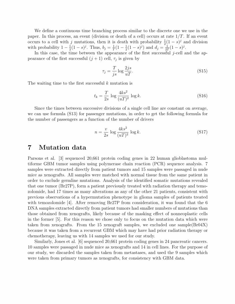
Parsons et al. [3] sequenced 20,661 protein coding genes in 22 human glioblastoma mul-tiforme GBM tumor samples using polymerase chain reaction (PCR) sequence analysis. 7samples were extracted directly from patient tumors and 15 samples were passaged in nudemice as xenografts. All samples were matched with normal tissue from the same patient inorder to exclude germline mutations. Analysis of the identified somatic mutations revealedthat one tumor (Br27P), form a patient previously treated with radiation therapy and temo-zolomide, had 17 times as many alterations as any of the other 21 patients, consistent withprevious observations of a hypermutation phenotype in glioma samples of patients treatedwith temozolomide [4]. After removing Br27P from consideration, it was found that the 6DNA samples extracted directly from patient tumors had smaller numbers of mutations thanthose obtained from xenografts, likely because of the masking e�ect of nonneoplastic cellsin the former [5]. For this reason we chose only to focus on the mutation data which weretaken from xenografts. From the 15 xenograft samples, we excluded one sample(Br04X)because it was taken from a recurrent GBM which may have had prior radiation therapy orchemotherapy, leaving us with 14 samples we used for our study.

Similarly, Jones et al. [6] sequenced 20,661 protein coding genes in 24 pancreatic cancers.10 samples were passaged in nude mice as xenografts and 14 in cell lines. For the purpose ofour study, we discarded the samples taken from metastases, and used the 9 samples whichwere taken from primary tumors as xenografts, for consistency with GBM data.

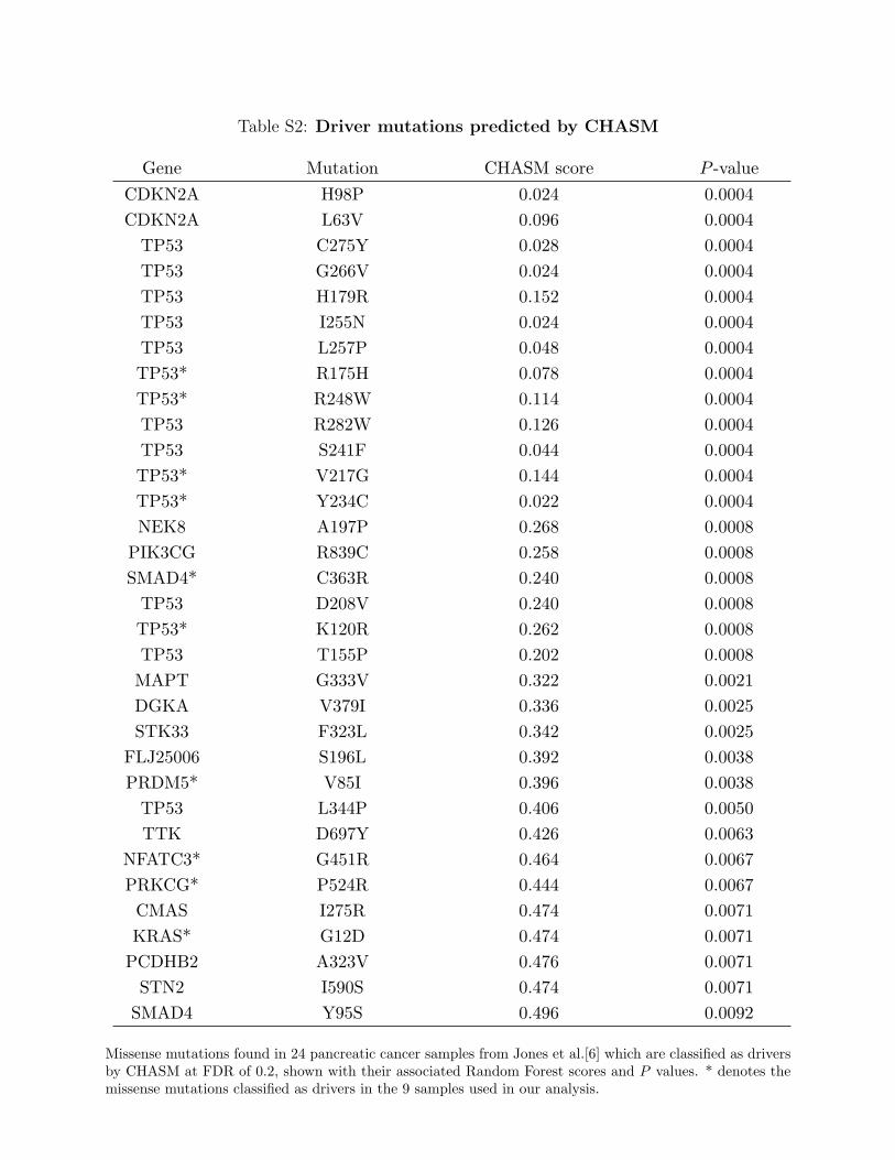
Table S2: Driver mutations predicted by CHASM

Gene Mutation CHASM score P -valueCDKN2A H98P 0.024 0.0004CDKN2A L63V 0.096 0.0004

TP53 C275Y 0.028 0.0004TP53 G266V 0.024 0.0004TP53 H179R 0.152 0.0004TP53 I255N 0.024 0.0004TP53 L257P 0.048 0.0004TP53* R175H 0.078 0.0004TP53* R248W 0.114 0.0004TP53 R282W 0.126 0.0004TP53 S241F 0.044 0.0004TP53* V217G 0.144 0.0004TP53* Y234C 0.022 0.0004NEK8 A197P 0.268 0.0008

PIK3CG R839C 0.258 0.0008SMAD4* C363R 0.240 0.0008

TP53 D208V 0.240 0.0008TP53* K120R 0.262 0.0008TP53 T155P 0.202 0.0008

MAPT G333V 0.322 0.0021DGKA V379I 0.336 0.0025STK33 F323L 0.342 0.0025

FLJ25006 S196L 0.392 0.0038PRDM5* V85I 0.396 0.0038

TP53 L344P 0.406 0.0050TTK D697Y 0.426 0.0063

NFATC3* G451R 0.464 0.0067PRKCG* P524R 0.444 0.0067CMAS I275R 0.474 0.0071KRAS* G12D 0.474 0.0071

PCDHB2 A323V 0.476 0.0071STN2 I590S 0.474 0.0071

SMAD4 Y95S 0.496 0.0092

Missense mutations found in 24 pancreatic cancer samples from Jones et al.[6] which are classified as driversby CHASM at FDR of 0.2, shown with their associated Random Forest scores and P values. * denotes themissense mutations classified as drivers in the 9 samples used in our analysis.

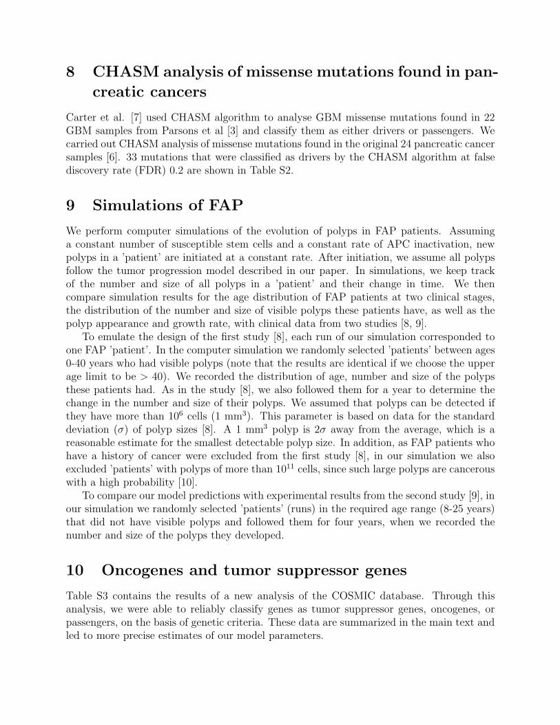
8 CHASM analysis of missense mutations found in pan-creatic cancers

Carter et al. [7] used CHASM algorithm to analyse GBM missense mutations found in 22GBM samples from Parsons et al [3] and classify them as either drivers or passengers. Wecarried out CHASM analysis of missense mutations found in the original 24 pancreatic cancersamples [6]. 33 mutations that were classified as drivers by the CHASM algorithm at falsediscovery rate (FDR) 0.2 are shown in Table S2.

9 Simulations of FAP

We perform computer simulations of the evolution of polyps in FAP patients. Assuminga constant number of susceptible stem cells and a constant rate of APC inactivation, newpolyps in a ’patient’ are initiated at a constant rate. After initiation, we assume all polypsfollow the tumor progression model described in our paper. In simulations, we keep trackof the number and size of all polyps in a ’patient’ and their change in time. We thencompare simulation results for the age distribution of FAP patients at two clinical stages,the distribution of the number and size of visible polyps these patients have, as well as thepolyp appearance and growth rate, with clinical data from two studies [8, 9].

To emulate the design of the first study [8], each run of our simulation corresponded toone FAP ’patient’. In the computer simulation we randomly selected ’patients’ between ages0-40 years who had visible polyps (note that the results are identical if we choose the upperage limit to be > 40). We recorded the distribution of age, number and size of the polypsthese patients had. As in the study [8], we also followed them for a year to determine thechange in the number and size of their polyps. We assumed that polyps can be detected ifthey have more than 106 cells (1 mm3). This parameter is based on data for the standarddeviation (�) of polyp sizes [8]. A 1 mm3 polyp is 2� away from the average, which is areasonable estimate for the smallest detectable polyp size. In addition, as FAP patients whohave a history of cancer were excluded from the first study [8], in our simulation we alsoexcluded ’patients’ with polyps of more than 1011 cells, since such large polyps are cancerouswith a high probability [10].

To compare our model predictions with experimental results from the second study [9], inour simulation we randomly selected ’patients’ (runs) in the required age range (8-25 years)that did not have visible polyps and followed them for four years, when we recorded thenumber and size of the polyps they developed.

10 Oncogenes and tumor suppressor genes

Table S3 contains the results of a new analysis of the COSMIC database. Through thisanalysis, we were able to reliably classify genes as tumor suppressor genes, oncogenes, orpassengers, on the basis of genetic criteria. These data are summarized in the main text andled to more precise estimates of our model parameters.

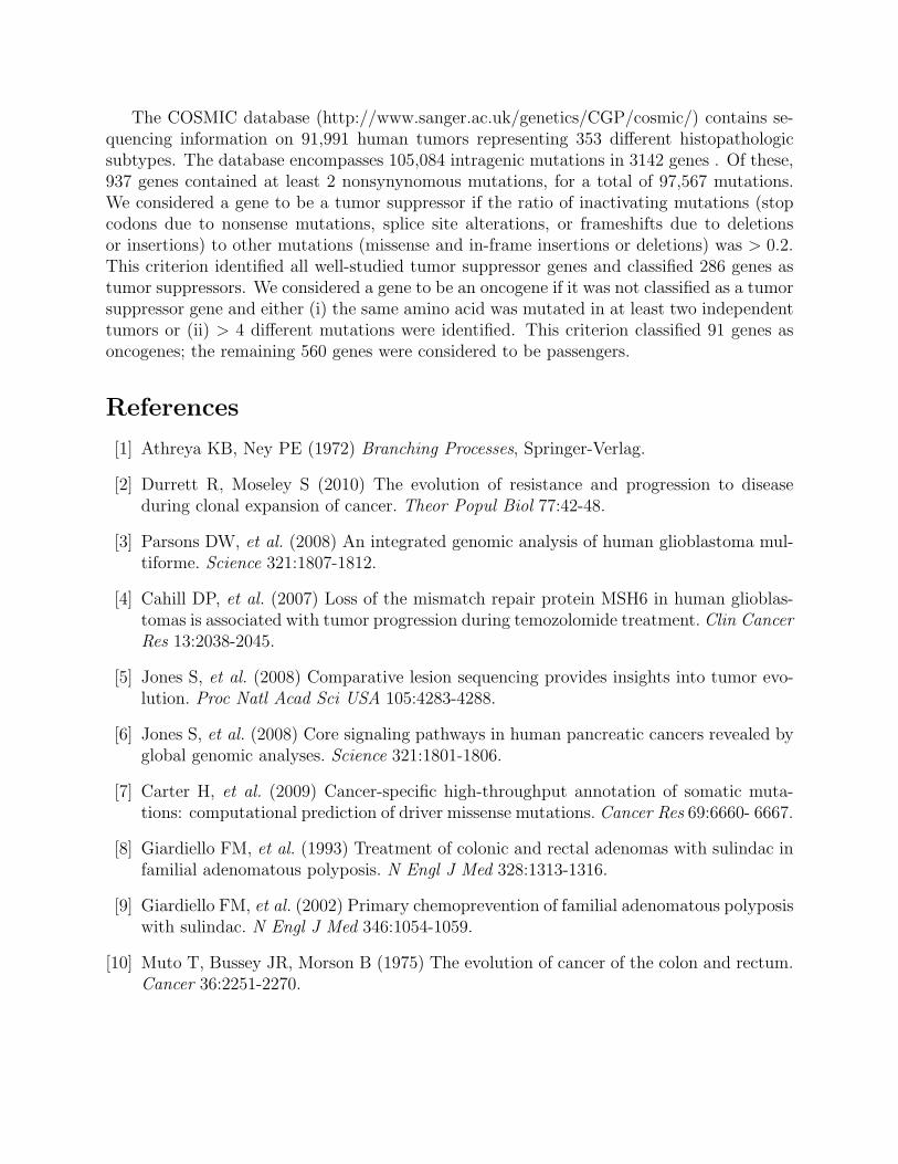
The COSMIC database (http://www.sanger.ac.uk/genetics/CGP/cosmic/) contains se-quencing information on 91,991 human tumors representing 353 di�erent histopathologicsubtypes. The database encompasses 105,084 intragenic mutations in 3142 genes . Of these,937 genes contained at least 2 nonsynynomous mutations, for a total of 97,567 mutations.We considered a gene to be a tumor suppressor if the ratio of inactivating mutations (stopcodons due to nonsense mutations, splice site alterations, or frameshifts due to deletionsor insertions) to other mutations (missense and in-frame insertions or deletions) was > 0.2.This criterion identified all well-studied tumor suppressor genes and classified 286 genes astumor suppressors. We considered a gene to be an oncogene if it was not classified as a tumorsuppressor gene and either (i) the same amino acid was mutated in at least two independenttumors or (ii) > 4 di�erent mutations were identified. This criterion classified 91 genes asoncogenes; the remaining 560 genes were considered to be passengers.

References

[1] Athreya KB, Ney PE (1972) Branching Processes, Springer-Verlag.

[2] Durrett R, Moseley S (2010) The evolution of resistance and progression to diseaseduring clonal expansion of cancer. Theor Popul Biol 77:42-48.

[3] Parsons DW, et al. (2008) An integrated genomic analysis of human glioblastoma mul-tiforme. Science 321:1807-1812.

[4] Cahill DP, et al. (2007) Loss of the mismatch repair protein MSH6 in human glioblas-tomas is associated with tumor progression during temozolomide treatment. Clin CancerRes 13:2038-2045.

[5] Jones S, et al. (2008) Comparative lesion sequencing provides insights into tumor evo-lution. Proc Natl Acad Sci USA 105:4283-4288.

[6] Jones S, et al. (2008) Core signaling pathways in human pancreatic cancers revealed byglobal genomic analyses. Science 321:1801-1806.

[7] Carter H, et al. (2009) Cancer-specific high-throughput annotation of somatic muta-tions: computational prediction of driver missense mutations. Cancer Res 69:6660- 6667.

[8] Giardiello FM, et al. (1993) Treatment of colonic and rectal adenomas with sulindac infamilial adenomatous polyposis. N Engl J Med 328:1313-1316.

[9] Giardiello FM, et al. (2002) Primary chemoprevention of familial adenomatous polyposiswith sulindac. N Engl J Med 346:1054-1059.

[10] Muto T, Bussey JR, Morson B (1975) The evolution of cancer of the colon and rectum.Cancer 36:2251-2270.

Gene

SymbolCancer Gene Type Accession Number

Truncating

mutations/gene

Missense

mutations/gene

Recurrent

mutations/gene

ABL1 Oncogene X16416 0 214 183

ABL2 Tumor Suppressor Gene NM_005158 2 2 0

ACVR1B Tumor Suppressor Gene NM_020328 4 0 2

ACVR2A Tumor Suppressor Gene NM_001616 9 1 8

ADAM29 Tumor Suppressor Gene NM_014269.2 1 3 0

ADAM33 Tumor Suppressor Gene NM_025220.2 1 1 0

ADAMTS18 Tumor Suppressor Gene NM_199355.1 2 4 0

ADAMTS20 Tumor Suppressor Gene NM_025003.2 1 3 0

ADAMTSL3 Oncogene NM_207517.1 1 7 0

ADH7 Tumor Suppressor Gene NM_000673.3 1 1 0

ADHFE1 Tumor Suppressor Gene NM_144650.1 1 2 0

AKAP6 Oncogene NM_004274.3 0 6 0

AKAP9 Tumor Suppressor Gene NM_147171.1 2 5 0

AKT1 Oncogene NM_005163 0 62 61

ALK Oncogene NM_004304 1 77 65

ALOX15 Tumor Suppressor Gene NM_001140.3 1 1 0

ALPK2 Tumor Suppressor Gene NM_052947 1 2 0

ALPK3 Tumor Suppressor Gene NM_020778 1 2 0

ALS2 Tumor Suppressor Gene NM_020919.2 1 1 0

ANAPC5 Tumor Suppressor Gene NM_016237.3 1 4 0

APBB1IP Tumor Suppressor Gene NM_019043.3 1 4 0

APC Tumor Suppressor Gene NM_000038 1691 161 1435

APOB Tumor Suppressor Gene ENST00000233242 1 2 0

ARHGAP29 Tumor Suppressor Gene NM_004815.2 2 5 1

ARHGAP6 Tumor Suppressor Gene NM_013427.1 1 1 0

ARHGEF11 Tumor Suppressor Gene NM_198236.1 1 1 0

ARID1A Tumor Suppressor Gene NM_006015.3 1 1 0

ASXL1 Tumor Suppressor Gene ENST00000358956 9 4 3

ATM Tumor Suppressor Gene NM_000051 56 141 47

ATR Tumor Suppressor Gene NM_001184 2 5 0

ATRX Tumor Suppressor Gene NM_138271.1 1 3 0

AURKA Tumor Suppressor Gene NM_003600 1 2 0

AXL Tumor Suppressor Gene NM_001699 1 4 0

BAI3 Oncogene NM_001704.1 0 8 0

BAZ1A Tumor Suppressor Gene NM_013448.2 1 3 0

BCL11A Oncogene NM_022893.2 0 7 0

BCORL1 Tumor Suppressor Gene NM_021946.2 1 1 0

BIRC6 Tumor Suppressor Gene NM_016252.1 2 5 0

BMPR1A Tumor Suppressor Gene NM_004329 1 2 0

BRAF Oncogene NM_004333 7 12523 12466

BRCA1 Tumor Suppressor Gene NM_007294.1 21 5 1

BRCA2 Tumor Suppressor Gene NM_000059.1 21 13 1

BRD2 Tumor Suppressor Gene NM_005104 1 4 0

BRD3 Tumor Suppressor Gene NM_007371 1 2 0

C14orf115 Tumor Suppressor Gene ENST00000256362 1 1 0

C9orf96 Tumor Suppressor Gene SU_SgK071 1 1 0

CAD Tumor Suppressor Gene NM_004341.2 1 4 0

CASK Tumor Suppressor Gene NM_003688 1 1 0

CBL Oncogene NM_005188.1 2 80 60

CD248 Tumor Suppressor Gene ENST00000311330 1 1 0

CDC42BPA Tumor Suppressor Gene NM_014826.3 1 1 0

CDC42BPB Tumor Suppressor Gene NM_006035 1 3 0

CDC7 Tumor Suppressor Gene NM_003503.2 3 0 2

CDC73 Tumor Suppressor Gene NM_024529.3 33 3 7

CDH1 Tumor Suppressor Gene NM_004360.2 90 80 47

CDKL2 Tumor Suppressor Gene NM_003948 1 2 0

CDKN2A Tumor Suppressor Gene NM_000077 1190 1532 2481

CDS1 Tumor Suppressor Gene ENST00000295887 1 1 0

CEBPA Tumor Suppressor Gene NM_004364.2 328 287 397

CENPF Tumor Suppressor Gene ENST00000366955 1 1 0

CENTB1 Tumor Suppressor Gene ENST00000158762 1 2 0

CENTD3 Tumor Suppressor Gene NM_022481.4 1 3 0

Table S3: Oncogenes and tumor suppressor genes

CES3 Tumor Suppressor Gene ENST00000303334 1 1 0

CHD5 Oncogene NM_015557.1 0 5 0

CHD8 Tumor Suppressor Gene XM_370738.2 1 2 0

CHEK1 Tumor Suppressor Gene NM_001274 1 1 0

CHUK Tumor Suppressor Gene NM_001278 5 0 2

CIC Tumor Suppressor Gene ENST00000160740 1 2 0

CLSPN Tumor Suppressor Gene NM_022111.2 1 2 0

CNTN1 Tumor Suppressor Gene NM_001843.2 1 1 0

COL11A1 Oncogene ENST00000358392 0 3 1

COL14A1 Tumor Suppressor Gene NM_021110.1 2 4 0

COL1A1 Tumor Suppressor Gene ENST00000225964 1 3 0

COL7A1 Tumor Suppressor Gene ENST00000328333 1 3 0

CSF1R Oncogene NM_005211 5 36 33

CSMD3 Tumor Suppressor Gene NM_198123.1 5 17 1

CTNNA1 Tumor Suppressor Gene NM_001903.2 6 0 0

CTNNB1 Oncogene NM_001904 23 2369 2221

CTNND2 Tumor Suppressor Gene NM_001332.2 1 2 0

CTSH Tumor Suppressor Gene ENST00000220166 1 1 0

CUBN Tumor Suppressor Gene ENST00000377833 1 4 0

CXorf30 Tumor Suppressor Gene XM_098980.6 1 1 0

CYB5D2 Oncogene ENST00000301391 0 2 1

CYLD Tumor Suppressor Gene NM_015247.1 5 1 0

DBF4 Tumor Suppressor Gene NM_006716.3 2 0 2

DBN1 Tumor Suppressor Gene ENST00000309007 1 2 0

DCLK3 Oncogene SU_DCAMKL3 0 6 0

DDR2 Tumor Suppressor Gene NM_006182 1 1 0

DEPDC2 Tumor Suppressor Gene NM_024870.2 2 5 0

DGKB Oncogene NM_004080.1 0 7 0

DGKG Tumor Suppressor Gene NM_001346.1 1 2 0

DIP2C Tumor Suppressor Gene ENST00000280886 2 3 0

DLC1 Tumor Suppressor Gene NM_182643.1 1 1 0

DNAH8 Oncogene NM_001371.1 1 5 0

DPH4 Tumor Suppressor Gene ENST00000395949 1 1 0

DPYSL4 Oncogene ENST00000338492 0 2 1

DYRK2 Tumor Suppressor Gene NM_006482 1 1 0

EGFL6 Oncogene NM_015507.2 0 2 1

EGFR Oncogene NM_005228 11 5214 5028

EIF2AK1 Tumor Suppressor Gene NM_014413 1 1 0

ELP2 Tumor Suppressor Gene NM_018255.1 2 1 1

EP300 Oncogene NM_001429.1 0 5 0

EP400 Tumor Suppressor Gene ENST00000389562 1 2 0

EPHA3 Oncogene NM_005233 0 8 0


EPHA6 Oncogene SU_EPHA6 0 6 0


EPHB1 Tumor Suppressor Gene NM_004441 2 3 0

EPHB6 Oncogene NM_004445 0 6 0

ERBB2 Oncogene NM_004448 1 100 64

ERCC6 Oncogene NM_000124.1 0 6 2

ERGIC3 Tumor Suppressor Gene ENST00000279052 1 1 0

ERN1 Oncogene NM_001433 1 5 0

ERN2 Tumor Suppressor Gene NM_033266.1 2 0 0

EVC2 Tumor Suppressor Gene ENST00000344408 1 2 0

EVI1 Tumor Suppressor Gene ENST00000264674 1 1 0

EXOC4 Tumor Suppressor Gene ENST00000253861 1 2 0

EZH2 Tumor Suppressor Gene NM_004456.3 2 0 0

F2RL2 Tumor Suppressor Gene NM_004101.2 1 1 0

FAM123B Tumor Suppressor Gene NM_152424.1 20 47 46

FBXW7 Tumor Suppressor Gene NM_033632.1 45 198 177

FGFR1 Oncogene NM_000604 0 6 0

FGFR2 Oncogene NM_022970 1 7 0

FGFR3 Oncogene NM_000142 8 1892 1862

FKTN Oncogene ENST00000223528 0 2 1

FLNB Oncogene ENST00000295956 0 5 0

FLT3 Oncogene Z26652 1 6833 6740

FN1 Oncogene ENST00000336916 0 6 0

FOXL2 Oncogene NM_023067.2 0 95 93

FRAP1 Oncogene NM_004958 1 7 0

FYN Tumor Suppressor Gene NM_002037 1 2 0

G3BP2 Tumor Suppressor Gene ENST00000395719 1 1 0

GATA1 Tumor Suppressor Gene NM_002049.2 158 25 115

GEN1 Tumor Suppressor Gene ENST00000317402 2 1 0

GLI1 Oncogene NM_005269.1 0 6 0

GLI3 Tumor Suppressor Gene NM_000168.2 1 4 0

GNAQ Oncogene NM_002072.2 1 131 129

GNAS Oncogene NM_000516.3 0 240 237

GOLIM4 Oncogene ENST00000309027 0 4 1

GPR124 Tumor Suppressor Gene ENST00000021763 1 1 0

GPR81 Tumor Suppressor Gene ENST00000356987 2 0 0

GRK5 Tumor Suppressor Gene NM_005308 1 1 0

GUCY2F Tumor Suppressor Gene NM_001522 1 4 0

HAPLN1 Tumor Suppressor Gene ENST00000380141 1 1 0

HDAC4 Tumor Suppressor Gene NM_006037.2 3 2 1

HDLBP Tumor Suppressor Gene NM_005336.2 1 2 0

HERC1 Tumor Suppressor Gene NM_003922.1 1 1 0

HERC6 Tumor Suppressor Gene NM_017912.3 1 1 0

HIF1A Tumor Suppressor Gene NM_001530.2 2 1 0

HNF1A Tumor Suppressor Gene NM_000545.3 56 50 55

HRAS Oncogene NM_005343 2 605 592

ICK Tumor Suppressor Gene NM_016513 1 1 0

IDH1 Oncogene NM_005896.2 0 890 887

IDH2 Oncogene NM_002168.2 0 43 41

IGF1R Tumor Suppressor Gene NM_000875 1 3 0

IKBKAP Tumor Suppressor Gene NM_003640.2 1 3 0

IKBKB Tumor Suppressor Gene SU_IKKb 1 1 0

IKZF3 Tumor Suppressor Gene NM_012481.3 1 2 0

ING4 Tumor Suppressor Gene ENST00000341550 1 1 0

ITGA10 Tumor Suppressor Gene NM_003637.3 1 2 0

ITGA9 Tumor Suppressor Gene NM_002207.2 1 2 0

ITGB2 Tumor Suppressor Gene NM_000211.1 3 1 0



ITK Tumor Suppressor Gene NM_005546 1 3 0

ITPR2 Oncogene NM_002223.1 0 7 0

ITSN2 Tumor Suppressor Gene NM_006277.1 2 0 0

JAK2 Oncogene NM_004972 1 23281 23237

JAK3 Oncogene NM_000215 1 18 7

JARID1A Tumor Suppressor Gene NM_005056.1 2 0 0

JARID1C Tumor Suppressor Gene NM_004187.1 6 2 0

KIAA0182 Tumor Suppressor Gene NM_014615.1 1 1 0

KIAA1409 Tumor Suppressor Gene ENST00000256339 2 0 1

KIF16B Oncogene NM_024704.3 0 5 0

KIT Oncogene NM_000222 67 3572 3445

KNTC1 Tumor Suppressor Gene NM_014708.3 2 2 0

KRAS Oncogene NM_004985 3 14828 14796

LAMC1 Tumor Suppressor Gene NM_002293.2 1 1 0

LAMP1 Tumor Suppressor Gene ENST00000332556 1 1 0

LATS2 Tumor Suppressor Gene NM_014572 1 1 0

LDHB Tumor Suppressor Gene NM_002300.3 2 0 1

LRRC7 Tumor Suppressor Gene ENST00000035383 1 1 0

LRRK2 Tumor Suppressor Gene SU_LRRK2 2 3 0

LTBP1 Tumor Suppressor Gene NM_206943.1 2 0 0

LTF Tumor Suppressor Gene ENST00000231751 1 1 0

MACF1 Tumor Suppressor Gene ENST00000360115 1 2 0

MAMDC4 Tumor Suppressor Gene ENST00000317446 1 2 0

MAP2K4 Tumor Suppressor Gene NM_003010 7 10 2





MAPK13 Tumor Suppressor Gene NM_002754 1 1 0

MARK1 Tumor Suppressor Gene NM_018650.1 1 2 0

MARK4 Tumor Suppressor Gene NM_031417 1 1 0

MAST4 Tumor Suppressor Gene SU_MAST4 2 4 0

MCM3AP Tumor Suppressor Gene NM_003906.3 1 2 0

MEN1 Tumor Suppressor Gene ENST00000312049 128 63 51

MET Oncogene NM_000245 5 111 82

MEX3B Tumor Suppressor Gene NM_032246.3 1 1 0

MGA Tumor Suppressor Gene XM_031689.7 2 3 0

MGC16169 Tumor Suppressor Gene SU_TBCK 1 2 0

MGC42105 Tumor Suppressor Gene NM_153361 2 2 1

MICAL1 Tumor Suppressor Gene ENST00000358807 1 1 0

MINK1 Tumor Suppressor Gene NM_015716 2 1 0

MLH1 Tumor Suppressor Gene NM_000249.2 28 22 16

MLL Tumor Suppressor Gene NM_005933.1 2 5 0

MLL2 Oncogene ENST00000301067 2 15 0



MMP16 Tumor Suppressor Gene NM_005941.2 1 1 0

MMP2 Oncogene NM_004530.1 0 5 0

MPL Oncogene NM_005373.1 1 241 232

MSH2 Tumor Suppressor Gene NM_000251.1 28 11 7

MSH6 Tumor Suppressor Gene NM_000179.1 98 33 86

MTMR3 Tumor Suppressor Gene NM_021090.2 1 1 0

MYH11 Tumor Suppressor Gene ENST00000338282 1 1 0

MYH9 Oncogene ENST00000216181 1 6 1

MYLK2 Tumor Suppressor Gene NM_033118 1 2 0

MYO1B Oncogene ENST00000392317 0 2 1

N4BP2 Tumor Suppressor Gene NM_018177.2 2 2 0

NBN Tumor Suppressor Gene NM_002485.3 2 1 0

NCDN Oncogene ENST00000373253 0 2 1

NCOA7 Tumor Suppressor Gene NM_181782.2 1 1 0

NEK10 Oncogene SU_NEK10 0 5 0

NEK11 Tumor Suppressor Gene NM_024800.2 1 3 0

NEK7 Tumor Suppressor Gene NM_133494 1 1 0

NEK8 Tumor Suppressor Gene SU_NEK8 1 2 0

NEK9 Tumor Suppressor Gene NM_033116.3 1 1 0

NF1 Tumor Suppressor Gene ENST00000358273 132 31 40

NF2 Tumor Suppressor Gene NM_000268.2 546 67 322

NFKB1 Tumor Suppressor Gene NM_003998.2 2 0 1

NIN Tumor Suppressor Gene NM_016350.3 1 1 0

NIPBL Tumor Suppressor Gene NM_133433.2 2 2 0

NLE1 Tumor Suppressor Gene NM_018096.2 2 1 1

NLRP1 Tumor Suppressor Gene NM_033004.2 2 2 0

NLRP5 Tumor Suppressor Gene ENST00000390649 1 1 0

NLRP8 Oncogene ENST00000291971 0 5 0

NOTCH1 Tumor Suppressor Gene NM_017617.2 184 442 447

NOTCH2 Tumor Suppressor Gene NM_024408.2 8 4 3

NPM1 Tumor Suppressor Gene NM_002520.4 2167 7 2161

NRAS Oncogene NM_002524 1 2118 2099

NRBP1 Tumor Suppressor Gene NM_013392 1 1 0

NRK Tumor Suppressor Gene SU_ZC4-NRK 1 2 0

NTRK3 Oncogene NM_002530 0 7 0

NUP214 Tumor Suppressor Gene NM_005085.2 1 3 0

NUP98 Tumor Suppressor Gene NM_016320.2 1 4 0

OBSCN Tumor Suppressor Gene SU_OBSCN.1 4 12 0

ODZ1 Oncogene ENST00000262800.1 0 9 0

PAK7 Tumor Suppressor Gene NM_020341 1 4 0

PARP1 Tumor Suppressor Gene NM_001618.2 1 1 0

PDGFRA Oncogene NM_006206 4 498 452

PDK3 Tumor Suppressor Gene NM_005391 1 1 0

PDZRN4 Tumor Suppressor Gene NM_013377.2 1 3 0

PER1 Tumor Suppressor Gene ENST00000317276 1 4 0

PHF14 Tumor Suppressor Gene NM_001007157.1 2 1 0

PHOX2B Tumor Suppressor Gene ENST00000381741 4 1 1

PIK3CA Oncogene NM_006218.1 19 2105 1998

PIK3R1 Oncogene NM_181523.1 1 9 0

PIM2 Tumor Suppressor Gene NM_006875 1 1 0

PKHD1 Oncogene ENST00000371117 0 5 0

POLN Tumor Suppressor Gene NM_181808.1 1 2 0

PRKAR1A Tumor Suppressor Gene NM_212472.1 4 2 0

PRKCA Tumor Suppressor Gene NM_002737 1 3 0

PRKD2 Tumor Suppressor Gene NM_016457 1 3 0

PRKDC Oncogene NM_006904 0 9 0

PTCH1 Tumor Suppressor Gene NM_000264.2 162 109 84

PTEN Tumor Suppressor Gene NM_000314.4 961 691 1200

PTPN11 Oncogene NM_002834.3 0 372 347

PTPN9 Tumor Suppressor Gene NM_002833.2 1 1 0

PTPRC Oncogene NM_002838.2 0 6 1

PTPRT Oncogene NM_133170.2 0 5 0

RAD18 Tumor Suppressor Gene NM_020165.2 2 1 1



RAD54B Tumor Suppressor Gene NM_012415.2 1 1 0

RASA3 Tumor Suppressor Gene NM_007368.2 1 1 0

RASGRF2 Oncogene NM_006909.1 0 5 0

RB1 Tumor Suppressor Gene NM_000321 206 33 93

RET Oncogene NM_020975 0 346 311

REV3L Tumor Suppressor Gene NM_002912.1 1 1 0

RFC4 Tumor Suppressor Gene NM_002916.3 1 2 0

RFX2 Tumor Suppressor Gene ENST00000303657 1 2 0

RGL2 Tumor Suppressor Gene NM_004761.2 1 1 0

RIF1 Oncogene NM_018151.1 0 5 0

RNF123 Tumor Suppressor Gene NM_022064.2 1 2 0

ROCK1 Tumor Suppressor Gene NM_005406 2 1 0

ROCK2 Tumor Suppressor Gene NM_004850 2 1 0

ROR1 Oncogene NM_005012 1 6 0

ROR2 Tumor Suppressor Gene NM_004560 1 3 0

ROS1 Oncogene NM_002944 1 5 0

RPS6KA2 Tumor Suppressor Gene NM_021135 2 2 0

RUNX1 Tumor Suppressor Gene ENST00000300305 86 120 105

SENP6 Tumor Suppressor Gene NM_015571.1 1 2 0

SERPINA2 Tumor Suppressor Gene XM_372532.2 1 1 0

SETD2 Tumor Suppressor Gene ENST00000330022 12 3 0

SFRS6 Tumor Suppressor Gene ENST00000244020 1 1 0

SGK3 Tumor Suppressor Gene NM_013257 1 1 0

SgK494 Tumor Suppressor Gene SU_SgK494 1 3 0

SgK495 Tumor Suppressor Gene SU_SgK495 2 2 0

SMAD2 Tumor Suppressor Gene NM_005901.3 2 1 0



SMARCA4 Tumor Suppressor Gene NM_003072.2 11 15 0

SMARCB1 Tumor Suppressor Gene NM_003073.2 146 86 154

SMC6 Tumor Suppressor Gene NM_024624.2 2 1 0

SMG1 Tumor Suppressor Gene SU_SMG1 1 4 0

SMO Oncogene NM_005631.3 0 28 11

SNF1LK Tumor Suppressor Gene NM_173354 1 2 0

SNX13 Tumor Suppressor Gene NM_015132.2 1 1 0

SOCS1 Tumor Suppressor Gene NM_003745.1 24 31 11

SORL1 Tumor Suppressor Gene ENST00000260197 1 4 0

SOX11 Tumor Suppressor Gene ENST00000322002 1 1 0

SPEG Tumor Suppressor Gene SU_SPEG 1 3 0

SPEN Oncogene NM_015001.2 1 5 0

SPO11 Tumor Suppressor Gene ENST00000371263 1 1 0

SPTAN1 Tumor Suppressor Gene ENST00000372731 1 4 0

SRC Tumor Suppressor Gene NM_005417 11 0 10

SRPK2 Tumor Suppressor Gene BC035214 1 1 0

STK11 Tumor Suppressor Gene NM_000455 95 85 85


STK32B Tumor Suppressor Gene NM_018401 2 1 0

STK32C Tumor Suppressor Gene SU_YANK3 1 1 0


SUFU Tumor Suppressor Gene NM_016169.2 3 1 0

SYNE1 Oncogene ENST00000265368 0 5 0

SYNE2 Tumor Suppressor Gene ENST00000358025 1 2 0

TAF1 Tumor Suppressor Gene NM_138923 2 6 0

TAF1L Tumor Suppressor Gene NM_153809 5 6 1

TCF12 Tumor Suppressor Gene NM_207037.1 4 0 1

TCF7L2 Tumor Suppressor Gene ENST00000369397 2 1 1

TECTA Tumor Suppressor Gene ENST00000392793 1 3 0

TEX14 Oncogene SU_SgK307 0 6 0

TGFBR2 Tumor Suppressor Gene NM_003242 4 7 1

TMEM161A Oncogene ENST00000162044 0 2 1

TMPRSS6 Tumor Suppressor Gene ENST00000346753 1 2 0

TNFAIP3 Tumor Suppressor Gene NM_006290.2 68 34 32

TNFRSF8 Oncogene NM_001243.2 0 2 1

TNK2 Tumor Suppressor Gene NM_005781 2 4 0

TNKS2 Tumor Suppressor Gene AF264912.1 1 4 0

TNNI3K Tumor Suppressor Gene NM_015978 2 3 0

TNPO1 Tumor Suppressor Gene NM_002270.2 2 2 0

TNPO3 Tumor Suppressor Gene NM_012470.2 1 1 0

TOP2B Tumor Suppressor Gene NM_001068.2 1 2 0

TP53 Tumor Suppressor Gene NM_000546 164 449 423

TPO Tumor Suppressor Gene NM_000547.3 1 2 0

TRIM33 Tumor Suppressor Gene NM_015906 3 3 0

TRIM36 Tumor Suppressor Gene NM_018700.2 1 2 0

TRIO Oncogene NM_007118.2 1 8 0

TRIP11 Tumor Suppressor Gene ENST00000267622 1 3 0

TRRAP Oncogene NM_003496 0 13 0

TSC1 Tumor Suppressor Gene NM_000368.2 3 1 0

TSHR Oncogene NM_000369.1 0 263 234

TTBK2 Tumor Suppressor Gene SU_TTBK2 1 1 0

TTK Tumor Suppressor Gene NM_003318 5 0 4

TTN Oncogene NM_003319 3 61 0

TWF2 Tumor Suppressor Gene NM_007284 1 1 0

TYK2 Tumor Suppressor Gene BC014243 1 1 0

UBP1 Tumor Suppressor Gene NM_014517.2 1 1 0

UBR4 Tumor Suppressor Gene NM_020765.1 5 6 0

UBR5 Oncogene NM_015902.4 0 5 0

ULK2 Tumor Suppressor Gene NM_014683 2 2 1

USP24 Tumor Suppressor Gene XM_371254.3 2 3 0

USP54 Tumor Suppressor Gene NM_152586.2 1 1 0

UTX Tumor Suppressor Gene NM_021140.1 23 4 18

VEPH1 Tumor Suppressor Gene ENST00000392832 2 1 0

VHL Tumor Suppressor Gene NM_000551.2 727 483 870

VPS13B Oncogene NM_017890.3 1 6 0

WNK1 Oncogene NM_018979 0 5 0

WNK2 Tumor Suppressor Gene SU_WNK2 3 3 0

WNK4 Tumor Suppressor Gene NM_032387 1 3 0

WRN Tumor Suppressor Gene ENST00000298139.1 1 1 0

WT1 Tumor Suppressor Gene NM_024426.2 222 65 194

XRCC6 Tumor Suppressor Gene NM_001469.2 2 0 1

ZC3H12B Tumor Suppressor Gene NM_001010888.1 1 1 0

ZMYM4 Tumor Suppressor Gene NM_005095.2 2 1 0

ZNF384 Tumor Suppressor Gene ENST00000361959 1 2 0

Accumulation of driver and passenger mutations during ...antal/Mypapers/accum10.pdf · Accumulation...

Documents

Transcript of Accumulation of driver and passenger mutations during ...antal/Mypapers/accum10.pdf · Accumulation...