MANAGERIAL ACCOUNTING

Table of Contents TABLE OF CONTENTS 1

MANAGERIAL ACCOUNTING AND COST CONCEPTS 6 MANUFACTURING COSTS 6 PRODUCT COSTS VS PERIOD COSTS 6 COST CLASSIFICATIONS FOR PREDICTING COST BEHAVIOR 7 THE ANALYSIS OF MIXED COSTS 10 THE HIGH-LOW METHOD 11 THE LEAST-SQUARES REGRESSION METHOD 12 TRADITIONAL AND CONTRIBUTION FORMAT INCOME STATEMENTS 13 TRADITIONAL FORMAT INCOME STATEMENT 13 CONTRIBUTION FORMAT INCOME STATEMENT 13 COST CLASSIFICATIONS FOR ASSIGNING COSTS TO COST OBJECTS 13 DIRECT COST 14 INDIRECT COST 14 COST CLASSIFICATIONS FOR DECISION MAKING 14 DIFFERENTIAL COST AND REVENUE 14 OPPORTUNITY COST 14 SUNK COST 14 LEAST-SQUARES REGRESSION COMPUTATIONS 14 COST OF QUALITY 15 QUALITY OF CONFORMANCE 15 PREVENTION COSTS 15 APPRAISAL COSTS 15 INTERNAL FAILURE COSTS 15 EXTERNAL FAILURE COSTS 16 QUALITY COST REPORTS 16 USE OF QUALITY COST INFORMATION 16 INTERNATIONAL ASPECTS OF QUALITY 17 ISO 9000 STANDARDS 17

JOB-ORDER COSTING 18 MEASURING DIRECT MATERIAL COST 18 JOB COST SHEET 18 MEASURING DIRECT LABOR COST 18 COMPUTING PREDETERMINED OVERHEAD RATES 18 APPLYING MANUFACTURING OVERHEAD 19 THE FLOW OF COSTS 20 APPLYING MANUFACTURING OVERHEAD 21 THE CONCEPT OF A CLEARING ACCOUNT 21 NONMANUFACTURING COSTS 22 COST OF GOODS MANUFACTURED 22 COST OF GOODS SOLD 22 SCHEDULES OF COST OF GOODS MANUFACTURED AND COST OF GOODS SOLD 22 UNDERAPPLIED AND OVERAPPLIED OVERHEAD 23 DISPOSITION OF UNDERAPPLIED OR OVERAPPLIED OVERHEAD BALANCES 23 GENERAL MODEL OF PRODUCT COST FLOWS 24 MULTIPLE PREDETERMINED OVERHEAD RATES 24

PROCESS COSTING 26 COMPARISON OF JOB-ORDER AND PROCESS COSTING 26 COST FLOWS IN PROCESS COSTING 26 THE FLOW OF MATERIALS, LABOR, AND OVERHEAD COSTS 27 MATERIALS, LABOR, AND OVERHEAD COST ENTRIES 27 EQUIVALENT UNITS OF PRODUCTION 28 WEIGHTED-AVERAGE METHOD 28 COMPUTE AND APPLY COSTS 29 OPERATION COSTING 29 FIFO METHOD 29 EQUIVALENT UNITS – FIFO METHOD 30 WEIGHTED-AVERAGE VS FIFO METHODS 30 COST PER EQUIVALENT UNIT – FIFO METHOD 31 APPLYING COSTS – FIFO METHOD 31 COST RECONCILIATION REPORT – FIFO METHOD 31 SERVICE DEPARTMENT ALLOCATIONS 31

COST-VOLUME-PROFIT RELATIONSHIPS 33 CVP RELATIONSHIPS IN EQUATION FORM 33 CVP RELATIONSHIPS IN GRAPHIC FORM 34 CONTRIBUTION MARGIN RATIO (CM RATIO) 36 APPLICATIONS OF CVP CONCEPTS 37 TARGET PROFIT AND BREAK-EVEN ANALYSIS 37 THE EQUATION METHOD 38 THE FORMULA METHOD 38 TARGET PROFIT ANALYSIS IN TERMS OF SALES DOLLARS 38 BREAK-EVEN IN SALES DOLLARS 39 MARGIN OF SAFETY 39 CVP CONSIDERATIONS IN CHOOSING A COST STRUCTURE 39 OPERATING LEVERAGE 39 SALES MIX 40 ASSUMPTIONS OF CVP ANALYSIS 40

VARIABLE COSTING AND SEGMENT REPORTING 41 OVERVIEW OF VARIABLE AND ABSORPTION COSTING 41 VARIABLE COSTING 41 ABSORPTION COSTING 41 SELLING AND ADMINISTRATIVE EXPENSES 41 VARIABLE AND ABSORPTION COSTING 42 VARIABLE COSTING CONTRIBUTION FORMAT INCOME STATEMENT 43 ABSORPTION COSTING INCOME STATEMENT 43 RECONCILIATION OF VARIABLE COSTING WITH ABSORPTION COSTING INCOME 43 ADVANTAGES OF VARIABLE COSTING AND THE CONTRIBUTION APPROACH 45 THEORY OF CONSTRAINTS 46 SEGMENTED INCOME STATEMENTS AND THE CONTRIBUTION APPROACH 46 IDENTIFYING TRACEABLE FIXED COSTS 47 SEGMENTED INCOME STATEMENTS – COMMON MISTAKES 47

ACTIVITY-BASED COSTING: TOOL TO AID DECISION MAKING 49

NONMANUFACTURING COST AND ACTIVITY-BASED COSTING 49 MANUFACTURING COSTS AND ACTIVITY-BASED COSTING 49 COST POOLS, ALLOCATION BASES, AND ACTIVITY-BASED COSTING 49 DESIGNING AN ACTIVITY-BASED COSTING (ABC) SYSTEM 50 STEPS FOR IMPLEMENTING ACTIVITY-BASED COSTING 50 COMPARISON OF TRADITIONAL AND ABC PRODUCT COSTS 52 PRODUCT MARGINS COMPUTED USING THE TRADITIONAL COST SYSTEM 52 DIFFERENCE BETWEEN ABC AND TRADITIONAL PRODUCT COSTS 52 TARGETING PROCESS IMPROVEMENTS 52 ACTIVITY-BASED COSTING AND EXTERNAL REPORTS 53 THE LIMITATIONS OF ACTIVITY-BASED COSTING 53

STANDARD COSTS AND VARIANCES 54 STANDARD COSTS – SETTING THE STAGE 54 SETTING STANDARD COSTS 54 SETTING DIRECT MATERIALS STANDARDS 55 SETTING DIRECT LABOR STANDARDS 55 SETTING VARIABLE MANUFACTURING OVERHEAD STANDARDS 55 A GENERAL MODEL FOR STANDARD COST VARIANCE ANALYSIS 56 USING STANDARD COSTS – DIRECT MATERIALS VARIANCES 57 MATERIALS QUANTITY VARIANCE 57 MATERIALS PRICE VARIANCE 58 USING STANDARD COSTS – DIRECT LABOR VARIANCES 58 LABOR EFFICIENCY VARIANCE 58 LABOR RATE VARIANCE 59 USING STANDARD COSTS – VARIABLE MANUFACTURING OVERHEAD VARIANCES 59 MANUFACTURING OVERHEAD VARIANCES 59 AN IMPORTANT SUBTLETY IN THE MATERIALS VARIANCES 60 VARIANCE ANALYSIS AND MANAGEMENT BY EXCEPTION 61 EVALUATION OF CONTROLS BASED ON STANDARD COSTS 62 ADVANTAGES OF STANDARD COSTS 62 POTENTIAL PROBLEMS WITH THE USE OF STANDARD COSTS 62 PREDETERMINED OVERHEAD RATES AND OVERHEAD ANALYSIS IN A STANDARD COSTING SYSTEM 63 OVERHEAD APPLICATION IN A STANDARD COST SYSTEM 63 CAUTIONS IN FIXED OVERHEAD ANALYSIS 64 RECONCILING OVERHEAD VARIANCES AND UNDERAPPLIED OR OVERAPPLIED OVERHEAD 64

CAPITAL BUDGETING DECISIONS 65 CAPITAL BUDGETING – PLANNING INVESTMENTS 65 DISCOUNTED CASH FLOW – THE NET PRESENT VALUE METHOD 65 EMPHASIS ON CASH FLOWS 66 TYPICAL CASH INFLOWS 66 RECOVERY OF THE ORIGINAL INVESTMENT 67 SIMPLIFYING ASSUMPTIONS 67 CHOOSING A DISCOUNT RATE 67 DISCOUNTED CASH FLOWS – THE INTERNAL RATE OF RETURN METHOD 68 SALVAGE VALUE AND OTHER CASH FLOWS 68 USING THE INTERNAL RATE OF RETURN 68 THE COST OF CAPITAL AS A SCREENING TOOL 69

COMPARISON OF THE NET PRESENT VALUE AND INTERNAL RATE OF RETURN METHODS 69 EXPANDING THE NET PRESENT VALUE METHOD 69 THE TOTAL-COST APPROACH 69 THE INCREMENTAL-COST APPROACH 70 LEAST-COST DECISIONS 70 UNCERTAIN CASH FLOW 70 PREFERENCE DECISIONS – THE RANKING OF INVESTMENT PROJECTS 70 INTERNAL RATE OF RETURN METHOD 71 NET PRESENT VALUE METHOD 71 OTHER APPROACHES TO CAPITAL BUDGETING DECISIONS 71 THE PAYBACK METHOD 71 EVALUATION OF THE PAYBACK METHOD 71 AN EXTENDED EXAMPLE OF PAYBACK 72 PAYBACK AND UNEVEN CASH FLOWS 72 THE SIMPLE RATE OF RETURN METHOD 72 POSTAUDIT OF INVESTMENT PROJECTS 73 THE CONCEPT OF PRESENT VALUE 73 MATHEMATICS OF INTEREST 73 COMPUTATION OF PRESENT VALUE 73 INCOME TAXES IN CAPITAL BUDGETING DECISIONS 74 DEPRECIATION TAX SHIELD 74 EXAMPLE OF INCOME TAXES AND CAPITAL BUDGETING 75

Managerial Accounting and Cost Concepts

Manufacturing Costs Manufacturing companies separate manufacturing costs into three categories:

• Raw Materials: The materials that go into the final product. • Direct Materials: Those materials that become an integral part of the finished

product and whose costs can be conveniently traced to the finished product. • Indirect Materials: Materials such as solder and glue, which are included as part

of manufacturing overhead. Direct labor consists of labor costs that can be easily traced to individual units of product. Sometimes called touch labor because direct labor workers typically touch the product while it is being made. Indirect labor is labor costs that cannot be physically traced to particular products, or that can be traced only at great cost and inconvenience. Manufacturing overhead, the 3rd element of manufacturing cost, includes all manufacturing costs except direct materials and direct labor. Other names for manufacturing overhead include indirect manufacturing cost, factory overhead, and factory burden. Nonmanufacturing costs are often divided into 2 categories:

• Selling costs include all costs that are incurred to secure customer orders and get the finished product to the customers. Sometimes called order-getting and order-filling costs.

• Administrative costs include all costs associated with the general management of an organization rather than with manufacturing or selling.

Product costs vs Period costs Product costs include all costs involved in acquiring or making a product. For financial accounting purposes. Because product costs are initially assigned to inventories, they’re also known as Inventoriable costs. Period costs are all the costs that are not product costs. All selling and administrative expenses are treated as period costs. Prime cost is the sum of direct materials cost and direct labor cost.

Conversion cost is the sum of direct labor cost and manufacturing overhead cost. Conversion cost is used to describe direct labor and manufacturing overhead because these costs are incurred to convert materials into the finished product. Cost classifications for predicting cost behavior

Cost behavior refers to how a cost react to changes in the level of activity. Costs are often categorized as variable, fixed, or mixed. The relative proportion of each type of cost in an organization is known as its cost structure. Variable cost varies, in total, in direct proportion to changes in the level of activity. Examples of VC are cost of goods sold, direct materials, direct labor, variable elements of manufacturing overhead such as indirect materials, supplies, and power, and variable elements of selling and administrative expenses such as commissions and shipping costs.

For a cost to be variable, it must be variable with respect to something i.e. activity base: a measure of whatever causes the incurrence of a variable cost. AKA cost driver. Common AB’s are: direct labor-hours, machine-hours, units produced, and units sold. Other examples include number of miles driven by a salesperson, number of pounds of laundry cleaned by a hotel, etc. Unless stated otherwise, assume that the activity based under consideration is the total volume of goods and services provided by the organization. Fixed cost is a cost that remains constant, in total, regardless of changes in the level of activity. E.g.: straight-line depreciation, insurance, property taxes, rent, supervisory salaries, administrative salaries, and advertising. As a general rule, you’re forewarned against expressing fixed costs on an average per unit basis in internal reports because it creates the false impression that fixed costs are like variable costs and that total fixed costs actually change as the level of activity changes. For planning purposes, fixed costs can be viewed as either committed or discretionary.

• Committed fixed costs represent organizational investments with a multiyear planning horizon that can’t be significantly reduced even for short periods of time without making fundamental changes.

• Discretionary fixed costs (manufacturing fixed costs) usually arise from annual decisions by management to spend on certain fixed cost items.

The relevant range is the range of activity within which the assumption that cost behavior is strictly linear is reasonably valid. Outside of the relevant range, a fixed cost may no longer be strictly fixed or a variable cost may not be strictly variable.

Cost behavior patterns such as salaries employees are often called step-variable costs. Step-variable costs can often be adjusted quickly as conditions change. The width of the steps for step-variable costs is so narrow that these costs can be treated as variable costs for most purposes. A Mixed cost contains both variable and fixed cost elements. Mixed costs are also known as semivariable costs.

The relationship between a mixed cost and the level of activity can be solved with the equation:

𝑌 = 𝑎 + 𝑏𝑋 Y= The total mixed cost a= The total fixed cost (vertical intercept of the line) b= The variable cost per unit of activity (the slope of the line) X= The level of activity The analysis of mixed costs Methods used to estimate the fixed and variable components of a mixed cost

• Account analysis an account is classified as either variable or fixed based on the analyst’s prior knowledge of how the cost in the account behaves.

• Engineering approach to cost analysis involves a detailed analysis of what cost behavior should be, based on an industrial engineer’s evaluation of the production methods to be used, the materials specifications, labor requirements, equipment usage, production efficiency, power consumption, etc.

• High-low and least-squares regression methods estimate the fixed and variable elements of a mixed cost by analyzing past records of cost and activity data.

o The first step in either of these methods is to diagnose cost behavior with a scatter graph plot.

§ Cost is known as the dependent variable because the amount of cost incurred during a period depends on the level of activity for the period

§ Activity is known as the independent variable because it causes variations in the cost.

§ Cost behavior is considered linear whenever a straight line is a reasonable approximation for the relation between cost and activity

The high-low method is based on the rise-over-run formula for the slope of a straight line. Formula to estimate the variable cost:

𝑉𝑎𝑟𝑖𝑎𝑏𝑙𝑒𝐶𝑜𝑠𝑡 = 𝑆𝑙𝑜𝑝𝑒𝑜𝑓𝑡ℎ𝑒𝑙𝑖𝑛𝑒 =𝑅𝑖𝑠𝑒𝑅𝑢𝑛 =

𝑦2 − 𝑦1𝑥2 − 𝑥1

To analyze mixed costs with the high-low method, begin by identifying the period with the lowest level of activity and the period with the highest level of activity.

𝑉𝐶 =𝑦2 − 𝑦1𝑥2 − 𝑥1 =

𝐶𝑜𝑠𝑡𝑎𝑡𝑡ℎ𝑒ℎ𝑖𝑔ℎ𝑒𝑠𝑡𝑎𝑐𝑡𝑖𝑣𝑖𝑡𝑦𝑙𝑒𝑣𝑒𝑙 − 𝐶𝑜𝑠𝑡𝑎𝑡𝑡ℎ𝑒𝑙𝑜𝑤𝑒𝑠𝑡𝑎𝑐𝑡𝑖𝑣𝑖𝑡𝑦𝑙𝑒𝑣𝑒𝑙𝐻𝑖𝑔𝑎𝑐𝑡𝑖𝑣𝑖𝑡𝑦𝑙𝑒𝑣𝑒𝑙 − 𝐿𝑜𝑤𝑎𝑐𝑡𝑖𝑣𝑖𝑡𝑦𝑙𝑒𝑣𝑒𝑙

or

𝑉𝑎𝑟𝑖𝑎𝑏𝑙𝑒𝐶𝑜𝑠𝑡 =𝐶ℎ𝑎𝑛𝑔𝑒𝑖𝑛𝑐𝑜𝑠𝑡

𝐶ℎ𝑎𝑛𝑔𝑒𝑖𝑛𝑎𝑐𝑡𝑖𝑣𝑖𝑡𝑦

The variable cost is estimated by dividing the difference in cost between the high and low levels of activity by the change in activity between those two points. Once you know the variable cost you can determine the amount of fixed cost by taking the total cost at either the high or the low activity level and deducting the variable cost element.

𝐹𝑖𝑥𝑒𝑑𝑐𝑜𝑠𝑡𝑒𝑙𝑒𝑚𝑒𝑛𝑡 = 𝑇𝑜𝑡𝑎𝑙𝑐𝑜𝑠𝑡 − 𝑉𝑎𝑟𝑖𝑎𝑏𝑙𝑒𝑐𝑜𝑠𝑡𝑒𝑙𝑒𝑚𝑒𝑛𝑡 The costs at the highest and lowest levels of activity are always used to analyze mixed cost under the high-low method, since this data reflects the greatest possible variation in activity.

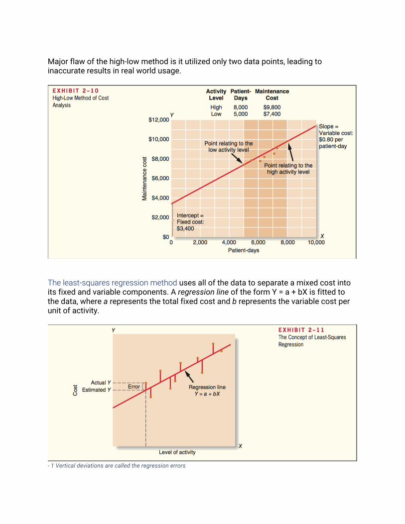
Major flaw of the high-low method is it utilized only two data points, leading to inaccurate results in real world usage.

The least-squares regression method uses all of the data to separate a mixed cost into its fixed and variable components. A regression line of the form Y = a + bX is fitted to the data, where a represents the total fixed cost and b represents the variable cost per unit of activity.

- 1 Vertical deviations are called the regression errors

Least-squares regression analysis generally provides more accurate cost estimates than the high-low methods because, rather than relying on just two data points, it uses all of the data points to fit a line that minimizes the sum of the squares errors. Traditional and contribution format income statements Traditional format income statement Traditional income statements are prepared primarily for external reporting purposes. It however has serious limitations when used for internal purposes as it doesn’t distinguish between fixed and variable costs.

• Gross margin = Sales – Cost of goods sold • Operating income = Gross margin – Selling and administrative expenses • Cost of goods sold (COGS) reports the product costs attached to the

merchandise sold during the period. • Selling and administrative expenses report all period costs that have been

expenses as incurred.

𝐶𝑂𝐺𝑆 = 𝐵𝑒𝑔𝑖𝑛𝑛𝑖𝑛𝑔𝑚𝑒𝑟𝑐ℎ𝑎𝑛𝑑𝑖𝑠𝑒𝑖𝑛𝑣𝑒𝑛𝑡𝑜𝑟𝑦 + 𝑃𝑢𝑟𝑐ℎ𝑎𝑠𝑒𝑠− 𝐸𝑛𝑑𝑖𝑛𝑔𝑚𝑒𝑟𝑐ℎ𝑎𝑛𝑑𝑖𝑠𝑒𝑖𝑛𝑣𝑒𝑛𝑡𝑜𝑟𝑦

Contribution format income statement The crucial distinction between fixed and variable cost is at the heart of the contribution approach to constructing income statements. Due to distinguishing fixed and variable costs it aids planning, controlling, and decision making. Thus it is used as an internal planning and decision-making tool, aiding cost-volume-profit analysis, management performance appraisals, and budgeting. The contribution approach separates costs into fixed and variable categories

Contribution margin = Sales – Variable Expenses a. For a merchandising company COGS is a variable cost that gets

included in the Variable Expenses portion of the contribution format income statement.

b. This amount contributes toward covering fixed expenses and then toward profits for the period.

Cost classifications for assigning costs to cost objects Costs are assigned to cost object for a variety of purposes including: pricing, preparing profitability studies, and controlling spending. Cost object: anything for which cost data are desired, including products, customers, jobs, and organizational subunits. For purposes of assigning costs to cost objects, costs are classified as either direct or indirect.

Direct cost Direct cost: a cost that can be easily and conveniently traced to a specified cost object. Indirect cost Indirect cost: a cost that cannot be easily and conveniently traced to a specified cost object. To be traced to a cost object such as a particular product, the cost must be caused by the cost object. Common cost: a (indirect) cost that is incurred to support a number of cost objects but cannot be traced to them individually. Cost classifications for decision making Differential cost and revenue Differential cost: A difference in cost between any two alternatives. Also known as an incremental cost. An incremental cost should refer only to an increase in cost from one alternative to another, a decremental cost refers to a decrease in cost. A differential cost is to an accountant what a marginal cost is to an economist. Differential cost can be either fixed or variable. Differential revenue: A difference in revenues between any two alternatives. In general, only the differences between alternatives are relevant in decisions. Those items that are the same under all alternatives and that are not affected by the decision can be ignored. Opportunity cost Opportunity cost is the potential benefit that is given up when one alternatives is selected over another. Sunk cost A sunk cost is a cost that has already been incurred and that cannot be changed by any decisions made now or in the future. Sunk costs are not differential costs. Only differential costs are relevant in a decision, sunk costs should always be ignored. Least-squares regression computations

The least-squares regression method for estimating a linear relation is based on the equation for a straight line: Y = a + bX Cost of quality Quality of conformance Quality of conformance: A product that meets or exceeds its design specifications and is free od defects that mar its appearance or degrade its performance. Preventing, detecting, and dealing with defects causes costs that are called quality costs or the cost of quality. Quality cost: all of the costs that are incurred to prevent defects or that result from defects in products. Prevention costs and appraisal costs are incurred in an effort to keep defective products from falling into the hands of customers. Internal failure costs and external failure costs are incurred because defects occur despite efforts to prevent them. Prevention costs Prevention costs support activities whose purpose is to reduce the number of defects. The most effective way to manage quality costs is to avoid having defects in the first place. Quality circles consist of small groups of employees that meet on a regular basis to discuss ways to improve quality. Both management and workers are included. Statistical process control is a technique that is used to detect whether a process is in or out of control. An out-of-control process results in defective units and may be caused by a miscalibrated machine or some other factor. Appraisal costs Appraisal costs, sometimes called inspection costs, are incurred to identify defective products before the products are shipped to customers. However, maintaining an army of inspectors is a costly, and ineffective, approach to quality control. Internal failure costs

Failure costs are incurred when a product fails to conform to its design specifications. Internal failure costs result from identifying defects before they are shipped to customers. External failure costs External failure costs result when a defective product is delivered to a customer. Quality cost reports A quality cost report details the prevention costs, appraisal costs, and costs of internal and external failures that arise from the company’s current quality control efforts.

Use of quality cost information A quality cost report has several uses:

• Helps managers see the financial significance of defects • Helps managers identify the relative importance of the quality problems faced by

the company • Helps managers see whether their quality costs are poorly distributed

3 limitations of quality cost information:

• Simply measuring and reporting quality costs does not solve quality problems • Results usually lag behind quality improvement programs

• The most important quality cost, lost sales arising from customer ill will, is usually omitted from the quality cost report because it is difficult to estimate

During the initial years of a quality improvement program, the benefits of compiling a quality cost report outweigh the costs and limitations of the report. International aspects of quality ISO 9000 standards The International Organization for Standardization (ISO) has established quality control guidelines known as the ISO 9000 standards. Suppliers must demonstrate to a certifying agency that:

1. A quality control system is in use, and the system clearly defines an expected level of quality

2. The system is fully operational and is backed up with detailed documentation of quality control procedures

3. The intended level of quality if being achieved on a sustained, consistent basis. The key to receiving certification under the ISO 9000 standards is documentation.

Job-Order Costing Absorption costing: All manufacturing costs, both fixed and variable, are assigned to units of product. Units are said to fully absorb manufacturing costs. Job-order costing is used in situation where many different products are produced each period. Examples of situations where job-order costing would be used include large-scale construction projects, commercial aircraft produced, cards designed and printed, airline meals prepared, etc. Job-order costing is also used extensively in service industries. Measuring direct material cost Bill of materials: a document that lists the type and quantity of each type of direct material needed to complete a unit of product. When an agreement has been reached with the customer concerning the quantities, prices, and shipment date for the order, a production order is issued. Materials requisition form: a document that specifies the type and quantity of materials to be drawn from the storeroom and identifies the job that will be charges for the cost of the materials. Job cost sheet A Job cost sheet records the materials, labor, and manufacturing overhead costs charged to that job. Measuring direct labor cost Direct labor consists of labor charges that are easily traced to a particular job. Labor charges that cannot be easily traced directly to any job are treated as part of the manufacturing overhead. A completed time ticket is an hour-by-hour summary of the employee’s activities throughout the day. Computing predetermined overhead rates Assigning manufacturing overhead to a specific job involves some difficulties because:

1. Manufacturing overhead is an indirect cost. 2. Manufacturing overhead consists of many different items 3. Because of the fixed costs in manufacturing overhead, total manufacturing

overhead costs tend to remain relatively constant from one period to the next, even though number of units produced can fluctuate.

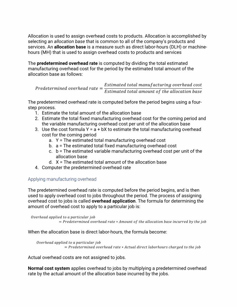
Allocation is used to assign overhead costs to products. Allocation is accomplished by selecting an allocation base that is common to all of the company’s products and services. An allocation base is a measure such as direct labor-hours (DLH) or machine-hours (MH) that is used to assign overhead costs to products and services The predetermined overhead rate is computed by dividing the total estimated manufacturing overhead cost for the period by the estimated total amount of the allocation base as follows:

𝑃𝑟𝑒𝑑𝑒𝑡𝑒𝑟𝑚𝑖𝑛𝑒𝑑𝑜𝑣𝑒𝑟ℎ𝑒𝑎𝑑𝑟𝑎𝑡𝑒 =𝐸𝑠𝑡𝑖𝑚𝑎𝑡𝑒𝑑𝑡𝑜𝑡𝑎𝑙𝑚𝑎𝑛𝑢𝑓𝑎𝑐𝑡𝑢𝑟𝑖𝑛𝑔𝑜𝑣𝑒𝑟ℎ𝑒𝑎𝑑𝑐𝑜𝑠𝑡𝐸𝑠𝑡𝑖𝑚𝑎𝑡𝑒𝑑𝑡𝑜𝑡𝑎𝑙𝑎𝑚𝑜𝑢𝑛𝑡𝑜𝑓𝑡ℎ𝑒𝑎𝑙𝑙𝑜𝑐𝑎𝑡𝑖𝑜𝑛𝑏𝑎𝑠𝑒

The predetermined overhead rate is computed before the period begins using a four-step process.

1. Estimate the total amount of the allocation base 2. Estimate the total fixed manufacturing overhead cost for the coming period and

the variable manufacturing overhead cost per unit of the allocation base 3. Use the cost formula Y = a + bX to estimate the total manufacturing overhead

cost for the coming period a. Y = The estimated total manufacturing overhead cost b. a = The estimated total fixed manufacturing overhead cost c. b = The estimated variable manufacturing overhead cost per unit of the

allocation base d. X = The estimated total amount of the allocation base

4. Computer the predetermined overhead rate Applying manufacturing overhead The predetermined overhead rate is computed before the period begins, and is then used to apply overhead cost to jobs throughout the period. The process of assigning overhead cost to jobs is called overhead application. The formula for determining the amount of overhead cost to apply to a particular job is: 𝑂𝑣𝑒𝑟ℎ𝑒𝑎𝑑𝑎𝑝𝑝𝑙𝑖𝑒𝑑𝑡𝑜𝑎𝑝𝑎𝑟𝑡𝑖𝑐𝑢𝑙𝑎𝑟𝑗𝑜𝑏

= 𝑃𝑟𝑒𝑑𝑒𝑡𝑒𝑟𝑚𝑖𝑛𝑒𝑑𝑜𝑣𝑒𝑟ℎ𝑒𝑎𝑑𝑟𝑎𝑡𝑒 ∗ 𝐴𝑚𝑜𝑢𝑛𝑡𝑜𝑓𝑡ℎ𝑒𝑎𝑙𝑙𝑜𝑐𝑎𝑡𝑖𝑜𝑛𝑏𝑎𝑠𝑒𝑖𝑛𝑐𝑢𝑟𝑟𝑒𝑑𝑏𝑦𝑡ℎ𝑒𝑗𝑜𝑏 When the allocation base is direct labor-hours, the formula become:

𝑂𝑣𝑒𝑟ℎ𝑒𝑎𝑑𝑎𝑝𝑝𝑙𝑖𝑒𝑑𝑡𝑜𝑎𝑝𝑎𝑟𝑡𝑖𝑐𝑢𝑙𝑎𝑟𝑗𝑜𝑏= 𝑃𝑟𝑒𝑑𝑒𝑡𝑒𝑟𝑚𝑖𝑛𝑒𝑑𝑜𝑣𝑒𝑟ℎ𝑒𝑎𝑑𝑟𝑎𝑡𝑒 ∗ 𝐴𝑐𝑡𝑢𝑎𝑙𝑑𝑖𝑟𝑒𝑐𝑡𝑙𝑎𝑏𝑜𝑟ℎ𝑜𝑢𝑟𝑠𝑐ℎ𝑎𝑟𝑔𝑒𝑑𝑡𝑜𝑡ℎ𝑒𝑗𝑜𝑏

Actual overhead costs are not assigned to jobs. Normal cost system applies overhead to jobs by multiplying a predetermined overhead rate by the actual amount of the allocation base incurred by the jobs.

A cost driver is a factor, such as machine-hours, beds occupied, computer time, or flight-hours that causes overhead costs. Most companies use direct labor-hours or direct labor cost as the allocation base for manufacturing overhead. Activity-based costing is designed to more accurately reflect the demands that products, customers, and other cost object make on overhead resources. Unit product cost is an average cost and should not be interpreted as the cost that would actually be incurred if another unit were produced. The flow of costs

Product costs flow through inventories on the balance sheet and then on to cost of goods sold in the income statement. Raw materials purchases are recorded in the Raw Materials inventory account. Raw materials include any materials that go into the final product. When used in production their costs are transferred to the Work in Process inventory account as direct materials. Work in process consists of units of product that are only partially complete and will require further work before they are ready for sale to the customer. Direct labor costs are added directly to Work in Process. Manufacturing overhead costs are applied to Work in Process by multiplying the predetermined overhead rate by the actual quantity

of the allocation based consumed by each job. When goods are completed, their costs are transferred from Work in Process to Finished Goods. Finished goods consist of completed units of product that have not yet been sold to customers. The amount transferred from Work in Process to Finished Goods is called cost of goods manufactured. Cost of goods manufactured includes the manufacturing costs associated with the goods that were finished during the period. As goods are sold, their costs are transferred from Finished Goods to Cost of Goods Sold. At this point, the various costs required to make the product are finally recorded as an expense. Until that point, these costs are in inventory accounts on the balance sheet. Period costs (selling and administrative expenses) do not flow through inventories on the balance sheet. They are recorded as expenses on the income statement in the period incurred.

• The materials charged to Work in Process represent direct materials for specific jobs.

• The Manufacturing Overhead account is separate from the Work in Process account. The purpose of the Manufacturing Overhead account is to accumulate all manufacturing overhead costs as they are incurred during a period.

• The Work in Process account summarizes all of the costs appearing on the job cost sheets of the jobs that are in process.

Applying manufacturing overhead Manufacturing overhead costs are assigned to Work in Process by means of the predetermined overhead rate. The predetermined overhead rate, established at the beginning of each year, is calculated by dividing the estimated total manufacturing overhead cost for the year by the estimated total amount of the allocation base. It is then used to apply overhead costs to jobs. The concept of a clearing account The Manufacturing Overhead account operates as a clearing account. Actual factory overhead costs are debited to the account as they are incurred throughout the year. When a job is completed, or at the end of the accounting period, overhead cost is applied to the job using the predetermined overhead rate, and Work in Process is debited and Manufacturing Overhead is credited. The predetermined overhead rate is based entirely on estimates of what the level of activity and overhead costs are expected to be, and it’s established before the year begins. The cost of a completed job consists of the actual direct materials cost of the job, the actual direct labor cost of the job, and the manufacturing overhead cost applied to the job.

Actual overhead costs are not charged to jobs; actual overhead costs do not appear on the job cost sheet nor do they appear in the Work in Process account. Only the applied overhead cost, based on the predetermined overhead rate, appears on the job cost sheet and in the Work in Process account. Nonmanufacturing costs Companies also incur selling and administrative costs. These costs should be treated as period expenses and charged directly to the income statement. Nonmanufacturing costs should not go into the Manufacturing Overhead account. Cost of goods manufactured When a job has been completed, it will have been charged with direct materials and direct labor cost, and manufacturing overhead will have been applied using the predetermined overhead rate. The costs of the completed job are transferred out of the Work in Process account and into the Finished Goods account. Cost of goods manufactured for the period = Sum of all amounts transferred between these two accounts. Cost of goods sold As finished goods are shipped to customers, their accumulated costs are transferred from the Finished Goods account to the Cost of Goods Sold account. Schedules of cost of goods manufactured and cost of goods sold Schedule of cost of goods manufactured contains 3 elements of product costs:

• Direct materials • Direct labor • Manufacturing overhead

And it summarizes the portions of those costs that remain in ending Work in Process inventory and that are transferred out of Work in Process into Finished Goods. Schedule of cost of goods sold contains 3 elements of product costs:

• Direct materials • Direct labor • Manufacturing overhead

And it summarizes the portions of those costs that remain in ending Finished Goods inventory and that are transferred out of Finished Goods into Cost of Goods Sold.

Schedule of cost of goods manufactured contains 3 keys aspects:

• 3 amounts are always added together to yield the total manufacturing costs: o Direct materials used in production (Included in total manufacturing costs

instead of raw material purchases) o Direct labor o Manufacturing overhead applied to work in process

• ManufacturingoverheadappliedtoWorkinProcess=thepredeterminedoverheadrate*theactualamountoftheallocationbaserecordedonalljobs. The actual manufacturing overhead costs incurred during the period are not added to the Work in Process account.

• 𝑇𝑜𝑡𝑎𝑙𝑚𝑎𝑛𝑢𝑓𝑎𝑐𝑡𝑢𝑟𝑖𝑛𝑔𝑐𝑜𝑠𝑡𝑠 + 𝑏𝑒𝑔𝑖𝑛𝑛𝑖𝑛𝑔𝑊𝑜𝑟𝑘𝑖𝑛𝑃𝑟𝑜𝑐𝑒𝑠𝑠𝑖𝑛𝑣𝑒𝑛𝑡𝑜𝑟𝑦 −𝑒𝑛𝑑𝑖𝑛𝑔𝑊𝑜𝑟𝑘𝑖𝑛𝑃𝑟𝑜𝑐𝑒𝑠𝑠𝑖𝑛𝑣𝑒𝑛𝑡𝑜𝑟𝑦 = 𝑐𝑜𝑠𝑡𝑜𝑓𝑔𝑜𝑜𝑑𝑠𝑚𝑎𝑛𝑢𝑓𝑎𝑐𝑡𝑢𝑟𝑒𝑑. Cost of goods manufactured represents the cost of goods completed during the period and transferred from Work in Process to Finished Goods.

Underapplied and Overapplied Overhead The overhead cost applied to Work in Process will generally differ from the amount of overhead cost actually incurred due to the predetermined overhead being applied before the period begins, and being based on estimated date. Underapplied or overapplied overhead: The difference between the overhead cost applied to Work in Process and the actual overhead costs of a period. Disposition of underapplied or overapplied overhead balances If there is a debit balance in the Manufacturing Overhead account of X dollars, then the overhead is underapplied by X dollars. If there is a credit balance in the Manufacturing Overhead account of Y dollars, then the overhead is overapplied by Y dollars. The underapplied or overapplied balance remaining in the Manufacturing Overhead account at the end of a period is treated in one of two ways:

1. Closed out to Cost of Goods Sold a. If, for example, the Manufacturing Overhead account has a debit balance,

Manufacturing Overhead must be credited to close out the account, thus increasing Cost of Goods Sold.

b. If overhead is underapplied, not enough cost will be applied to jobs, thus the cost of goods sold will be understated. Adding the underapplied overhead to the COGS corrects this understatement.

2. Allocated among the Work in Process, Finished Goods, and Cost of Goods Sold accounts in proportion to the overhead applied during the current period in ending balances.

a. Allocation of underapplied or overapplied overhead between Work in Process, Finished Goods, and COGS is more accurate than closing the entire balance into COGS.

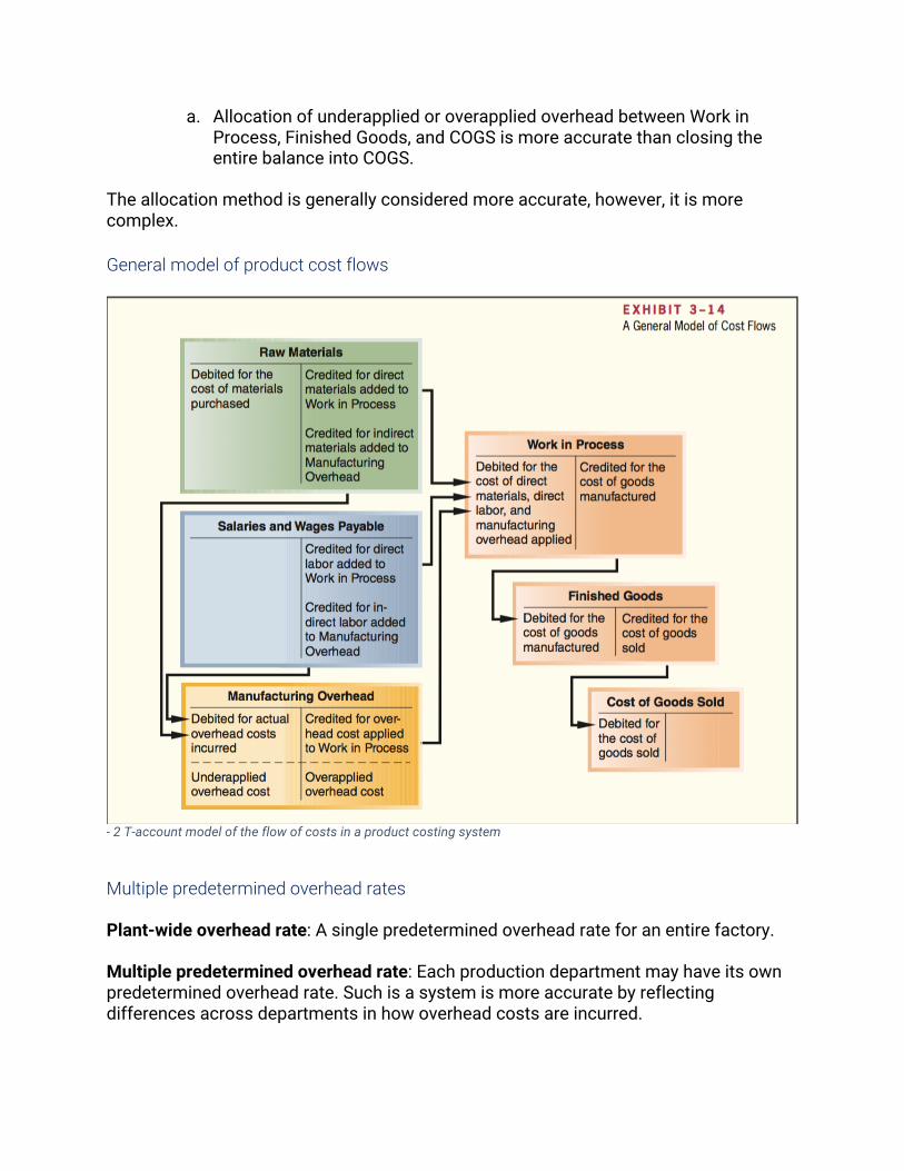
The allocation method is generally considered more accurate, however, it is more complex. General model of product cost flows

- 2 T-account model of the flow of costs in a product costing system

Multiple predetermined overhead rates Plant-wide overhead rate: A single predetermined overhead rate for an entire factory. Multiple predetermined overhead rate: Each production department may have its own predetermined overhead rate. Such is a system is more accurate by reflecting differences across departments in how overhead costs are incurred.

𝑃𝑟𝑒𝑑𝑒𝑡𝑒𝑟𝑚𝑖𝑛𝑒𝑑𝑜𝑣𝑒𝑟ℎ𝑒𝑎𝑑𝑟𝑎𝑡𝑒𝑏𝑎𝑠𝑒𝑑𝑜𝑛𝑐𝑎𝑝𝑎𝑐𝑖𝑡𝑦

=𝐸𝑠𝑡𝑖𝑚𝑎𝑡𝑒𝑑𝑡𝑜𝑡𝑎𝑙𝑚𝑎𝑛𝑢𝑓𝑎𝑐𝑡𝑢𝑟𝑖𝑛𝑔𝑜𝑣𝑒𝑟ℎ𝑒𝑎𝑑𝑐𝑜𝑠𝑡𝑎𝑡𝑐𝑎𝑝𝑎𝑐𝑖𝑡𝑦𝐸𝑠𝑡𝑖𝑚𝑎𝑡𝑒𝑑𝑡𝑜𝑡𝑎𝑙𝑎𝑚𝑜𝑢𝑛𝑡𝑜𝑓𝑡ℎ𝑒𝑎𝑙𝑙𝑜𝑐𝑎𝑡𝑖𝑜𝑛𝑏𝑎𝑠𝑒𝑎𝑡𝑐𝑎𝑝𝑎𝑐𝑖𝑡𝑦

Process Costing Process costing is used most commonly in industries that convert raw materials into homogeneous products, such as brick, soda, or paper, on a continuous basis. Comparison of job-order and process costing Similarities between job-order and process costing:

• Both have the same basic purpose o To assign material, labor, and manufacturing overhead costs to products o To provide a mechanism for computer unit product costs

• Both use the same basic manufacturing account o Manufacturing Overhead o Raw Materials o Work in Process o Finished Goods

• The flow of costs through the manufacturing accounts is basically the same in both systems.

Differences between job-order and process costing:

• Process costing is used when a company produces a continuous flow of units that are indistinguishable from one another.

o Job-order costing is used when a company produces many different jobs that have unique production requirements.

• Under Process costing, it makes no sense to try to identify materials, labor, and overhead costs with a particular customer order because each order is just one of many that are filled from a continuous flow of virtually identical units from the production line.

o Process costing accumulates costs by department, rather than by order, and assigns these costs uniformly to all units that pass through the departments during a period. Job cost sheets are not used to accumulate costs.

• Process costing systems compute unit costs by department o Job-order costing: unit costs are computer by job on the job cost sheet.

Cost flows in process costing Processing department: An organizational unit where work is performed on a product and where materials, labor, or overhead costs are added to the product.

The flow of materials, labor, and overhead costs In a process costing system, instead of having to trace costs to hundreds of different jobs, costs are traced to only a few processing departments.

Exhibit 4 – 3 important note:

1. A separate Work in Process account is maintained for each processing department. In a job-order costing system the entire company may have only 1 Work in Process account.

2. The completed production of the first processing department is transferred to the Work in Process account of the second processing department. After further work in Department B, the completed units are then transferred to Finished Goods.

3. Materials, labor, and overhead costs can be added in any processing department, not just the first.

Materials, labor, and overhead cost entries Material costs: As in job-order costing, materials are drawn from the storeroom using a materials requisition form. Materials can be added only in the first processing department, with subsequent departments adding only labor and overhead costs. Labor costs: In process costing, labor costs are traced to departments, not to individual jobs.

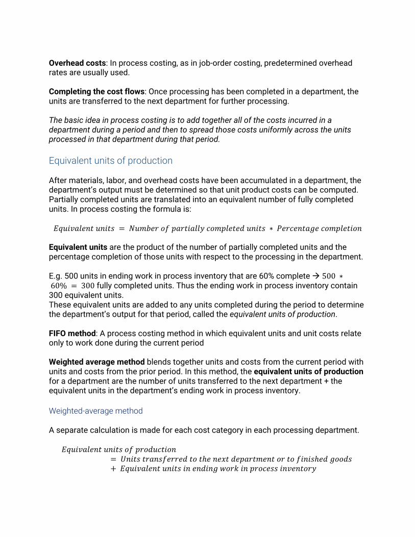
Overhead costs: In process costing, as in job-order costing, predetermined overhead rates are usually used. Completing the cost flows: Once processing has been completed in a department, the units are transferred to the next department for further processing. The basic idea in process costing is to add together all of the costs incurred in a department during a period and then to spread those costs uniformly across the units processed in that department during that period. Equivalent units of production After materials, labor, and overhead costs have been accumulated in a department, the department’s output must be determined so that unit product costs can be computed. Partially completed units are translated into an equivalent number of fully completed units. In process costing the formula is: 𝐸𝑞𝑢𝑖𝑣𝑎𝑙𝑒𝑛𝑡𝑢𝑛𝑖𝑡𝑠 = 𝑁𝑢𝑚𝑏𝑒𝑟𝑜𝑓𝑝𝑎𝑟𝑡𝑖𝑎𝑙𝑙𝑦𝑐𝑜𝑚𝑝𝑙𝑒𝑡𝑒𝑑𝑢𝑛𝑖𝑡𝑠 ∗ 𝑃𝑒𝑟𝑐𝑒𝑛𝑡𝑎𝑔𝑒𝑐𝑜𝑚𝑝𝑙𝑒𝑡𝑖𝑜𝑛

Equivalent units are the product of the number of partially completed units and the percentage completion of those units with respect to the processing in the department. E.g. 500 units in ending work in process inventory that are 60% complete à 500 ∗60% = 300 fully completed units. Thus the ending work in process inventory contain 300 equivalent units. These equivalent units are added to any units completed during the period to determine the department’s output for that period, called the equivalent units of production. FIFO method: A process costing method in which equivalent units and unit costs relate only to work done during the current period Weighted average method blends together units and costs from the current period with units and costs from the prior period. In this method, the equivalent units of production for a department are the number of units transferred to the next department + the equivalent units in the department’s ending work in process inventory. Weighted-average method A separate calculation is made for each cost category in each processing department.

𝐸𝑞𝑢𝑖𝑣𝑎𝑙𝑒𝑛𝑡𝑢𝑛𝑖𝑡𝑠𝑜𝑓𝑝𝑟𝑜𝑑𝑢𝑐𝑡𝑖𝑜𝑛= 𝑈𝑛𝑖𝑡𝑠𝑡𝑟𝑎𝑛𝑠𝑓𝑒𝑟𝑟𝑒𝑑𝑡𝑜𝑡ℎ𝑒𝑛𝑒𝑥𝑡𝑑𝑒𝑝𝑎𝑟𝑡𝑚𝑒𝑛𝑡𝑜𝑟𝑡𝑜𝑓𝑖𝑛𝑖𝑠ℎ𝑒𝑑𝑔𝑜𝑜𝑑𝑠+ 𝐸𝑞𝑢𝑖𝑣𝑎𝑙𝑒𝑛𝑡𝑢𝑛𝑖𝑡𝑠𝑖𝑛𝑒𝑛𝑑𝑖𝑛𝑔𝑤𝑜𝑟𝑘𝑖𝑛𝑝𝑟𝑜𝑐𝑒𝑠𝑠𝑖𝑛𝑣𝑒𝑛𝑡𝑜𝑟𝑦

The computation of the equivalent units of production involves adding the number of units transferred out of the department to the equivalent units in the department’s ending inventory. Each unit transferred out of the department is counted as one equivalent unit. Conversion cost = direct labor cost + manufacturing overhead cost. In process costing, conversion cost is often treated as a single element of a product cost. Compute and apply costs In the weighted-average method, the cost per equivalent unit is computed as follows:

𝐶𝑜𝑠𝑡𝑝𝑒𝑟𝑒𝑞𝑢𝑖𝑣𝑎𝑙𝑒𝑛𝑡𝑢𝑛𝑖𝑡

=𝐶𝑜𝑠𝑡𝑜𝑓𝑏𝑒𝑔𝑖𝑛𝑛𝑖𝑛𝑔𝑤𝑜𝑟𝑘𝑖𝑛𝑝𝑟𝑜𝑐𝑒𝑠𝑠𝑖𝑛𝑣𝑒𝑛𝑡𝑜𝑟𝑦 + 𝐶𝑜𝑠𝑡𝑎𝑑𝑑𝑒𝑑𝑑𝑢𝑟𝑖𝑛𝑔𝑡ℎ𝑒𝑝𝑒𝑟𝑖𝑜𝑑

𝐸𝑞𝑢𝑖𝑣𝑎𝑙𝑒𝑛𝑡𝑢𝑛𝑖𝑡𝑠𝑜𝑓𝑝𝑟𝑜𝑑𝑢𝑐𝑡𝑖𝑜𝑛

The numerator is the sum of the cost of beginning work in process inventory and of the cost added during the period. The weighted-average method blends together costs from the prior and current periods. It averages together units and costs from both the prior and current periods. The equivalent units are multiplied by the cost per equivalent unit to determine the cost assigned to the units. This is done for each cost category. Operation costing Operation costing is used in situations where products have some common characteristics and some individual characteristics. It employs aspects of both job-order and process costing.

• Products are typically processed in batches when operation costing used, while each batch charged for its own specific materials, thus being similar to job-order costing

• Labor and overhead costs are accumulated by operation or department, and these costs are assigned to units as in process costing.

FIFO method The FIFO method of process costing differs from the weighted-average method in 2 ways:

1. The computation of equivalent units 2. The way in which costs of beginning inventory are treated

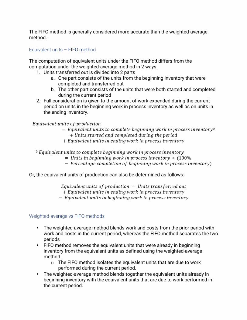
The FIFO method is generally considered more accurate than the weighted-average method. Equivalent units – FIFO method The computation of equivalent units under the FIFO method differs from the computation under the weighted-average method in 2 ways:

1. Units transferred out is divided into 2 parts a. One part consists of the units from the beginning inventory that were

completed and transferred out b. The other part consists of the units that were both started and completed

during the current period 2. Full consideration is given to the amount of work expended during the current

period on units in the beginning work in process inventory as well as on units in the ending inventory.

𝐸𝑞𝑢𝑖𝑣𝑎𝑙𝑒𝑛𝑡𝑢𝑛𝑖𝑡𝑠𝑜𝑓𝑝𝑟𝑜𝑑𝑢𝑐𝑡𝑖𝑜𝑛

= 𝐸𝑞𝑢𝑖𝑣𝑎𝑙𝑒𝑛𝑡𝑢𝑛𝑖𝑡𝑠𝑡𝑜𝑐𝑜𝑚𝑝𝑙𝑒𝑡𝑒𝑏𝑒𝑔𝑖𝑛𝑛𝑖𝑛𝑔𝑤𝑜𝑟𝑘𝑖𝑛𝑝𝑟𝑜𝑐𝑒𝑠𝑠𝑖𝑛𝑣𝑒𝑛𝑡𝑜𝑟𝑦º+𝑈𝑛𝑖𝑡𝑠𝑠𝑡𝑎𝑟𝑡𝑒𝑑𝑎𝑛𝑑𝑐𝑜𝑚𝑝𝑙𝑒𝑡𝑒𝑑𝑑𝑢𝑟𝑖𝑛𝑔𝑡ℎ𝑒𝑝𝑒𝑟𝑖𝑜𝑑

+𝐸𝑞𝑢𝑖𝑣𝑎𝑙𝑒𝑛𝑡𝑢𝑛𝑖𝑡𝑠𝑖𝑛𝑒𝑛𝑑𝑖𝑛𝑔𝑤𝑜𝑟𝑘𝑖𝑛𝑝𝑟𝑜𝑐𝑒𝑠𝑠𝑖𝑛𝑣𝑒𝑛𝑡𝑜𝑟𝑦

º𝐸𝑞𝑢𝑖𝑣𝑎𝑙𝑒𝑛𝑡𝑢𝑛𝑖𝑡𝑠𝑡𝑜𝑐𝑜𝑚𝑝𝑙𝑒𝑡𝑒𝑏𝑒𝑔𝑖𝑛𝑛𝑖𝑛𝑔𝑤𝑜𝑟𝑘𝑖𝑛𝑝𝑟𝑜𝑐𝑒𝑠𝑠𝑖𝑛𝑣𝑒𝑛𝑡𝑜𝑟𝑦= 𝑈𝑛𝑖𝑡𝑠𝑖𝑛𝑏𝑒𝑔𝑖𝑛𝑛𝑖𝑛𝑔𝑤𝑜𝑟𝑘𝑖𝑛𝑝𝑟𝑜𝑐𝑒𝑠𝑠𝑖𝑛𝑣𝑒𝑛𝑡𝑜𝑟𝑦 ∗ (100%− 𝑃𝑒𝑟𝑐𝑒𝑛𝑡𝑎𝑔𝑒𝑐𝑜𝑚𝑝𝑙𝑒𝑡𝑖𝑜𝑛𝑜𝑓𝑏𝑒𝑔𝑖𝑛𝑛𝑖𝑛𝑔𝑤𝑜𝑟𝑘𝑖𝑛𝑝𝑟𝑜𝑐𝑒𝑠𝑠𝑖𝑛𝑣𝑒𝑛𝑡𝑜𝑟𝑦)

Or, the equivalent units of production can also be determined as follows:

𝐸𝑞𝑢𝑖𝑣𝑎𝑙𝑒𝑛𝑡𝑢𝑛𝑖𝑡𝑠𝑜𝑓𝑝𝑟𝑜𝑑𝑢𝑐𝑡𝑖𝑜𝑛 = 𝑈𝑛𝑖𝑡𝑠𝑡𝑟𝑎𝑛𝑠𝑓𝑒𝑟𝑟𝑒𝑑𝑜𝑢𝑡+𝐸𝑞𝑢𝑖𝑣𝑎𝑙𝑒𝑛𝑡𝑢𝑛𝑖𝑡𝑠𝑖𝑛𝑒𝑛𝑑𝑖𝑛𝑔𝑤𝑜𝑟𝑘𝑖𝑛𝑝𝑟𝑜𝑐𝑒𝑠𝑠𝑖𝑛𝑣𝑒𝑛𝑡𝑜𝑟𝑦

−𝐸𝑞𝑢𝑖𝑣𝑎𝑙𝑒𝑛𝑡𝑢𝑛𝑖𝑡𝑠𝑖𝑛𝑏𝑒𝑔𝑖𝑛𝑛𝑖𝑛𝑔𝑤𝑜𝑟𝑘𝑖𝑛𝑝𝑟𝑜𝑐𝑒𝑠𝑠𝑖𝑛𝑣𝑒𝑛𝑡𝑜𝑟𝑦 Weighted-average vs FIFO methods

• The weighted-average method blends work and costs from the prior period with work and costs in the current period, whereas the FIFO method separates the two periods

• FIFO method removes the equivalent units that were already in beginning inventory from the equivalent units as defined using the weighted-average method.

o The FIFO method isolates the equivalent units that are due to work performed during the current period.

• The weighted-average method blends together the equivalent units already in beginning inventory with the equivalent units that are due to work performed in the current period.

Cost per equivalent unit – FIFO method In the FIFO method, the cost per equivalent unit is computed:

𝐶𝑜𝑠𝑡𝑝𝑒𝑟𝑒𝑞𝑢𝑖𝑣𝑎𝑙𝑒𝑛𝑡𝑢𝑛𝑖𝑡 =𝐶𝑜𝑠𝑡𝑎𝑑𝑑𝑒𝑑𝑑𝑢𝑟𝑖𝑛𝑔𝑡ℎ𝑒𝑝𝑒𝑟𝑖𝑜𝑑𝐸𝑞𝑢𝑖𝑣𝑎𝑙𝑒𝑛𝑡𝑢𝑛𝑖𝑡𝑠𝑜𝑓𝑝𝑟𝑜𝑑𝑢𝑐𝑡𝑖𝑜𝑛

In the FIFO method the cost per equivalent unit is based only on the costs incurred in the department in the current period. Applying costs – FIFO method The costs per equivalent unit are used to value units in ending inventory and units that are transferred to the next department. It’s more complicated than the weighted-average period because the cost of the units transferred out consists of three separate components:

1. The cost of beginning work in process inventory 2. The cost to complete the units in beginning work in process inventory 3. The cost of units started and completed during the period

Cost reconciliation report – FIFO method Total cost of units transferred out will be accounted for in the next department as costs transferred in. As in the weighted-average method, this cost will be treated in the process costing system as just another category of costs, like materials or conversion costs. The only difference is that the costs transferred in will always be 100% complete with respect to the work done in the ‘transferred in’ department. When the product are completed in the last department, their costs are transferred to finished goods. Service department allocations Most large organization have both operating departments and service departments. The central purposes of the organization are carried out in the operating departments. Service departments do not directly engage in operating activities; they provide services or assistance to the operating departments. In process costing, the processing departments are all operating departments. The overhead costs of operating departments commonly include allocations of costs from the service departments. If service department costs are classified as production

costs, they should be included in unit product costs and thus, must be allocated to operating departments in a process costing system. 3 approaches are used to allocate the cost of service departments to other departments

1. Direct method a. Ignores the services provided by a service department to other service

departments and allocates all service department costs directly to operating departments.

b. All costs are allocated directly to the operating departments c. Under the direct method, any of the allocation base attributable to the

service department themselves is ignored; only the amount of the allocation base attributable to the operating departments is used in the allocation.

d. After all allocations have been completed, all of the service department costs are contained in the two operating departments

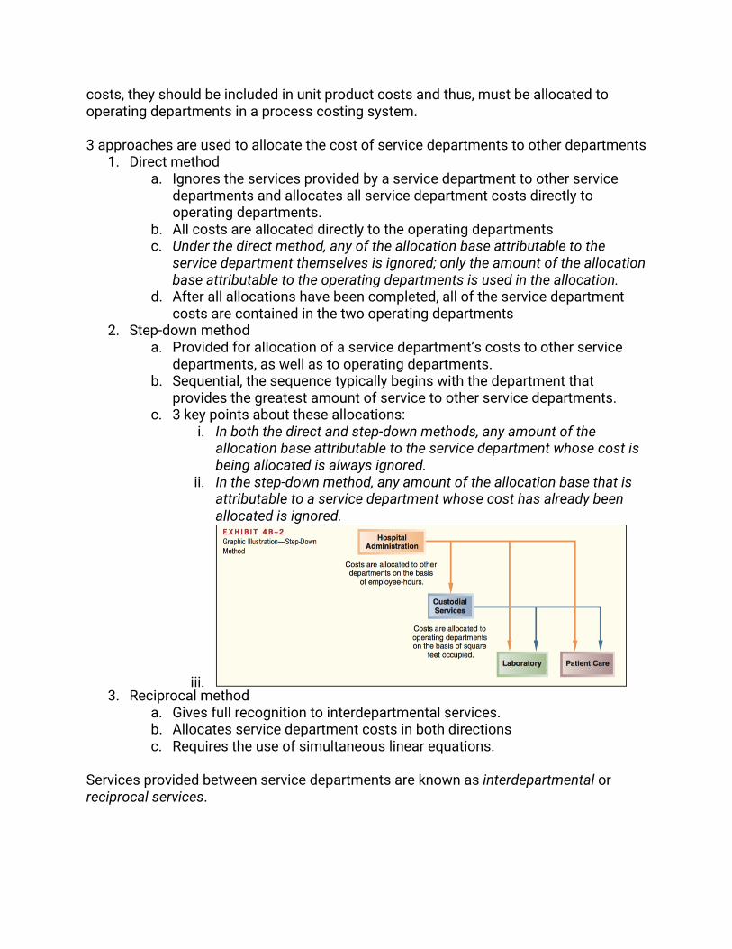
2. Step-down method a. Provided for allocation of a service department’s costs to other service

departments, as well as to operating departments. b. Sequential, the sequence typically begins with the department that

provides the greatest amount of service to other service departments. c. 3 key points about these allocations:

i. In both the direct and step-down methods, any amount of the allocation base attributable to the service department whose cost is being allocated is always ignored.

ii. In the step-down method, any amount of the allocation base that is attributable to a service department whose cost has already been allocated is ignored.

iii. 3. Reciprocal method

a. Gives full recognition to interdepartmental services. b. Allocates service department costs in both directions c. Requires the use of simultaneous linear equations.

Services provided between service departments are known as interdepartmental or reciprocal services.

Cost-Volume-Profit Relationships Cost-volume-profit (CVP) analysis focuses on how profits are affected by the following five factors:

1. Selling prices 2. Sales volume 3. Unit variable costs 4. Total fixed costs 5. Mix of products sold

𝐶𝑜𝑛𝑡𝑟𝑖𝑏𝑢𝑡𝑖𝑜𝑛𝑚𝑎𝑟𝑔𝑖𝑛 = 𝑠𝑎𝑙𝑒𝑠𝑟𝑒𝑣𝑒𝑛𝑢𝑒– 𝑣𝑎𝑟𝑖𝑎𝑏𝑙𝑒𝑒𝑥𝑝𝑒𝑛𝑠𝑒𝑠. Contribution margin is used first to cover the fixed expenses, and then whatever remains goes toward profits. If the contribution margin is not sufficient to cover the fixed expenses, a loss occurs for the period.

Break-even point is the level of sales at which profit is zero. Once the break-even point has been reached, net operating income will increase by the amount of the unit contribution margin for each additional unit sold. If sales are zero, the company’s loss would equal its fixed expenses. Each unit that is sold reduces the loss by the amount of the unit contribution margin. Once the break-even point has been reached, each additional unit sold increases the company’s profit by the amount of the unit contribution margin. CVP relationships in equation form The contribution format income statement can be expressed with the following equation:

𝑃𝑟𝑜𝑓𝑖𝑡 = (𝑆𝑎𝑙𝑒𝑠– 𝑉𝑎𝑟𝑖𝑎𝑏𝑙𝑒𝑒𝑥𝑝𝑒𝑛𝑠𝑒𝑠)– 𝐹𝑖𝑥𝑒𝑑𝑒𝑥𝑝𝑒𝑛𝑠𝑒𝑠 Profit stands for net operating income in equations.

When a company has only a single product, the equation becomes: Sales = Selling price per unit * Quantity sold = P * Q Variable expenses = Variable expenses per unit * Quantity sold = V * Q

𝑃𝑟𝑜𝑓𝑖𝑡 = (𝑃 ∗ 𝑄– 𝑉 ∗ 𝑄)– 𝐹𝑖𝑥𝑒𝑑𝑒𝑥𝑝𝑒𝑛𝑠𝑒𝑠 Express the simple profit equation in terms of the unit contribution margin: Unit CM = Selling price per unit – Variable expenses per unit = P – V Profit = (P * Q – V * Q) – Fixed expenses Profit = (P – V) * Q – Fixed expenses

𝑃𝑟𝑜𝑓𝑖𝑡 = 𝑈𝑛𝑖𝑡𝐶𝑀 ∗ 𝑄– 𝐹𝑖𝑥𝑒𝑑𝑒𝑥𝑝𝑒𝑛𝑠𝑒𝑠 CVP relationships in graphic form Cost-volume-profit (CVP) graph: Illustrates the relationship among revenue, cost, profit, and volume. A CVP graph highlights CVP relationships over wide ranges of activity. (Sometimes called a break-even chart) Preparing the CVP graph:

1. Draw a line parallel to the volume axis to represent total fixed expense. 2. Choose some volume of unit sales and plot the point representing total expense

at the sales volume you have selected. 3. Again choose some sales volume and plot the point representing total sales

dollars at the activity level you have selected.

The profit graph, an even simpler form of the CVP graph, is based on the following equation:

𝑃𝑟𝑜𝑓𝑖𝑡 = 𝑈𝑛𝑖𝑡𝐶𝑀 ∗ 𝑄– 𝐹𝑖𝑥𝑒𝑑𝑒𝑥𝑝𝑒𝑛𝑠𝑒𝑠

Contribution margin ratio (CM ratio) Contribution margin ratio (CM ratio): The contribution margin as a percentage of sales.

𝐶𝑀𝑟𝑎𝑡𝑖𝑜 =𝐶𝑜𝑛𝑡𝑟𝑖𝑏𝑢𝑡𝑖𝑜𝑛𝑚𝑎𝑟𝑔𝑖𝑛

𝑆𝑎𝑙𝑒𝑠 A change in sales on the contribution margin is expressed as:

𝐶ℎ𝑎𝑛𝑔𝑒𝑖𝑛𝑐𝑜𝑛𝑡𝑟𝑖𝑏𝑢𝑡𝑖𝑜𝑛𝑚𝑎𝑟𝑔𝑖𝑛 = 𝐶𝑀𝑟𝑎𝑡𝑖𝑜 ∗ 𝐶ℎ𝑎𝑛𝑔𝑒𝑖𝑛𝑠𝑎𝑙𝑒𝑠 The impact on net operating income of any given dollar change in total sales can be computer by applying the CM ratio in the dollar change. The relation between profit and the CM ratio can also be expressed using the following equation:

𝑃𝑟𝑜𝑓𝑖𝑡 = 𝐶𝑀𝑟𝑎𝑡𝑖𝑜 ∗ 𝑆𝑎𝑙𝑒𝑠– 𝐹𝑖𝑥𝑒𝑑𝑒𝑥𝑝𝑒𝑛𝑠𝑒𝑠 The previously mentioned equation can be derived using the basic profit equation and the definition of the CM ratio:

𝑃𝑟𝑜𝑓𝑖𝑡 = (𝑆𝑎𝑙𝑒𝑠– 𝑉𝑎𝑟𝑖𝑎𝑏𝑙𝑒𝑒𝑥𝑝𝑒𝑛𝑠𝑒𝑠)– 𝐹𝑖𝑥𝑒𝑑𝑒𝑥𝑝𝑒𝑛𝑠𝑒𝑠

𝑃𝑟𝑜𝑓𝑖𝑡 = 𝐶𝑜𝑛𝑡𝑟𝑖𝑏𝑢𝑡𝑖𝑜𝑛𝑚𝑎𝑟𝑔𝑖𝑛– 𝐹𝑖𝑥𝑒𝑑𝑒𝑥𝑝𝑒𝑛𝑠𝑒𝑠

𝑃𝑟𝑜𝑓𝑖𝑡 =𝐶𝑜𝑛𝑡𝑟𝑖𝑏𝑢𝑡𝑖𝑜𝑛𝑚𝑎𝑟𝑔𝑖𝑛

𝑆𝑎𝑙𝑒𝑠 ∗ 𝑆𝑎𝑙𝑒𝑠– 𝐹𝑖𝑥𝑒𝑑𝑒𝑥𝑝𝑒𝑛𝑠𝑒𝑠

𝑃𝑟𝑜𝑓𝑖𝑡 = 𝐶𝑀𝑟𝑎𝑡𝑖𝑜 ∗ 𝑆𝑎𝑙𝑒𝑠– 𝐹𝑖𝑥𝑒𝑑𝑒𝑥𝑝𝑒𝑛𝑠𝑒𝑠 ApplicationsofCVPconcepts Variable expense ratio: the ratio of variable expenses to sales.

𝑉𝑎𝑟𝑖𝑎𝑏𝑙𝑒𝑒𝑥𝑝𝑒𝑛𝑠𝑒𝑟𝑎𝑡𝑖𝑜 =𝑉𝑎𝑟𝑖𝑎𝑏𝑙𝑒𝑒𝑥𝑝𝑒𝑛𝑠𝑒𝑠

𝑆𝑎𝑙𝑒𝑠 For single product analysis:

𝑉𝑎𝑟𝑖𝑎𝑏𝑙𝑒𝑒𝑥𝑝𝑒𝑛𝑠𝑒𝑟𝑎𝑡𝑖𝑜 =𝑉𝑎𝑟𝑖𝑎𝑏𝑙𝑒𝑒𝑥𝑝𝑒𝑛𝑠𝑒𝑠𝑝𝑒𝑟𝑢𝑛𝑖𝑡

𝑈𝑛𝑖𝑡𝑠𝑒𝑙𝑙𝑖𝑛𝑔𝑝𝑟𝑖𝑐𝑒

Equation that relates the CM ratio to the variable expenses ratio:

𝐶𝑀𝑟𝑎𝑡𝑖𝑜 =𝐶𝑜𝑛𝑡𝑟𝑖𝑏𝑢𝑡𝑖𝑜𝑛𝑚𝑎𝑟𝑔𝑖𝑛

𝑆𝑎𝑙𝑒𝑠

𝐶𝑀𝑟𝑎𝑡𝑖𝑜 =𝑆𝑎𝑙𝑒𝑠 − 𝑉𝑎𝑟𝑖𝑎𝑏𝑙𝑒𝑒𝑥𝑝𝑒𝑛𝑠𝑒𝑠

𝑆𝑎𝑙𝑒𝑠

𝐶𝑀𝑟𝑎𝑡𝑖𝑜 = 1– 𝑉𝑎𝑟𝑖𝑎𝑏𝑙𝑒𝑒𝑥𝑝𝑒𝑛𝑠𝑒𝑟𝑎𝑡𝑖𝑜 ---Example on page 192-193 of books--- Incremental analysis considers only the revenue, cost, and volume that will change. Target profit and break-even analysis Target profit analysis: used to estimate what sales volume is needed to achieve a specific target profit.

The equation method We can use a basic profit equation to find the sales volume required to attain a target profit. If there is only one product we can use the contribution margin form of the equation:

𝑃𝑟𝑜𝑓𝑖𝑡 = 𝑈𝑛𝑖𝑡𝐶𝑀 ∗ 𝑄– 𝐹𝑖𝑥𝑒𝑑𝑒𝑥𝑝𝑒𝑛𝑠𝑒 The formula method The formula method is a short-cut version of the equation method. In a single-product situation, we can compute the sales volume required to attain a specific target profit using the formula:

𝑈𝑛𝑖𝑡𝑠𝑎𝑙𝑒𝑠𝑡𝑜𝑎𝑡𝑡𝑎𝑖𝑛𝑡ℎ𝑒𝑡𝑎𝑟𝑔𝑒𝑡𝑝𝑟𝑜𝑓𝑖𝑡 =𝑇𝑎𝑟𝑔𝑒𝑡𝑝𝑟𝑜𝑓𝑖𝑡 + 𝐹𝑖𝑥𝑒𝑑𝑒𝑥𝑝𝑒𝑛𝑠𝑒𝑠

𝑈𝑛𝑖𝑡𝐶𝑀 Previous formula derived as follows:

𝑃𝑟𝑜𝑓𝑖𝑡 = 𝑈𝑛𝑖𝑡𝐶𝑀 ∗ 𝑄– 𝐹𝑖𝑥𝑒𝑑𝑒𝑥𝑝𝑒𝑛𝑠𝑒𝑠𝑇𝑎𝑟𝑔𝑒𝑡𝑝𝑟𝑜𝑓𝑖𝑡 = 𝑈𝑛𝑖𝑡𝐶𝑀 ∗ 𝑄– 𝐹𝑖𝑥𝑒𝑑𝑒𝑥𝑝𝑒𝑛𝑠𝑒𝑠𝑈𝑛𝑖𝑡𝐶𝑀 ∗ 𝑄 = 𝑇𝑎𝑟𝑔𝑒𝑡𝑝𝑟𝑜𝑓𝑖𝑡 + 𝐹𝑖𝑥𝑒𝑑𝑒𝑥𝑝𝑒𝑛𝑠𝑒𝑠𝑄 = (𝑇𝑎𝑟𝑔𝑒𝑡𝑝𝑟𝑜𝑓𝑖𝑡 + 𝐹𝑖𝑥𝑒𝑑𝐸𝑥𝑝𝑒𝑛𝑠𝑒𝑠) ÷ 𝑈𝑛𝑖𝑡𝐶𝑀

Target profit analysis in terms of sales dollars

Several methods:

1. Solve for the unit sales to attain the target profit using the equation method or the formula method and then multiply the result by the selling price.

2. Solve for the required sales volume to attain the target profit using the basic equation stated in terms of the contribution margin ratio 𝑃𝑟𝑜𝑓𝑖𝑡 = 𝐶𝑀𝑟𝑎𝑡𝑖𝑜 ∗𝑠𝑎𝑙𝑒𝑠– 𝐹𝑖𝑥𝑒𝑑𝑒𝑥𝑝𝑒𝑛𝑠𝑒𝑠

𝐷𝑜𝑙𝑙𝑎𝑟𝑠𝑎𝑙𝑒𝑠𝑡𝑜𝑎𝑡𝑡𝑎𝑖𝑛𝑎𝑡𝑎𝑟𝑔𝑒𝑡𝑝𝑟𝑜𝑓𝑖𝑡 =𝑇𝑎𝑟𝑔𝑒𝑡𝑝𝑟𝑜𝑓𝑖𝑡 + 𝐹𝑖𝑥𝑒𝑑𝑒𝑥𝑝𝑒𝑛𝑠𝑒𝑠

𝐶𝑀𝑟𝑎𝑡𝑖𝑜 Previous formula derived as follows:

𝑃𝑟𝑜𝑓𝑖𝑡 = 𝐶𝑀𝑟𝑎𝑡𝑖𝑜 ∗ 𝑆𝑎𝑙𝑒𝑠– 𝐹𝑖𝑥𝑒𝑑𝑒𝑥𝑝𝑒𝑛𝑠𝑒𝑠𝑇𝑎𝑟𝑔𝑒𝑡𝑝𝑟𝑜𝑓𝑖𝑡 = 𝐶𝑀𝑟𝑎𝑡𝑖𝑜 ∗ 𝑆𝑎𝑙𝑒𝑠– 𝐹𝑖𝑥𝑒𝑑𝑒𝑥𝑝𝑒𝑛𝑠𝑒𝑠𝐶𝑀𝑟𝑎𝑡𝑖𝑜 ∗ 𝑆𝑎𝑙𝑒𝑠 = 𝑇𝑎𝑟𝑔𝑒𝑡𝑝𝑟𝑜𝑓𝑖𝑡 + 𝐹𝑖𝑥𝑒𝑑𝑒𝑥𝑝𝑒𝑛𝑠𝑒𝑠𝑆𝑎𝑙𝑒𝑠 = (𝑇𝑎𝑟𝑔𝑒𝑡𝑝𝑟𝑜𝑓𝑖𝑡 + 𝐹𝑖𝑥𝑒𝑑𝑒𝑥𝑝𝑒𝑛𝑠𝑒𝑠) ÷ 𝐶𝑀𝑟𝑎𝑡𝑖𝑜

Break-even in sales dollars Several methods:

1. Solve for the break-even point in unit sales using the equation method or the formula method and then multiply the result by the selling price.

2. Solve for the break-even point in sales dollars using the basic profit equation stated in terms of the contribution margin ratio or we can use the formula for the target profit.

𝐷𝑜𝑙𝑙𝑎𝑟𝑠𝑎𝑙𝑒𝑠𝑡𝑜𝑎𝑡𝑡𝑎𝑖𝑛𝑎𝑡𝑎𝑟𝑔𝑒𝑡𝑝𝑟𝑜𝑓𝑖𝑡 =𝑇𝑎𝑟𝑔𝑒𝑡𝑝𝑟𝑜𝑓𝑖𝑡 + 𝐹𝑖𝑥𝑒𝑑𝑒𝑥𝑝𝑒𝑛𝑠𝑒𝑠

𝐶𝑀𝑟𝑎𝑡𝑖𝑜

𝐷𝑜𝑙𝑙𝑎𝑟𝑠𝑎𝑙𝑒𝑠𝑡𝑜𝑏𝑟𝑒𝑎𝑘𝑒𝑣𝑒𝑛 =$0 + 𝐹𝑖𝑥𝑒𝑑𝑒𝑥𝑝𝑒𝑛𝑠𝑒𝑠

𝐶𝑀𝑟𝑎𝑡𝑖𝑜

𝐷𝑜𝑙𝑙𝑎𝑟𝑠𝑎𝑙𝑒𝑠𝑡𝑜𝑏𝑟𝑒𝑎𝑘𝑒𝑣𝑒𝑛 =𝐹𝑖𝑥𝑒𝑑𝑒𝑥𝑝𝑒𝑛𝑠𝑒𝑠

𝐶𝑀𝑟𝑎𝑡𝑖𝑜 Margin of safety Margin of safety: The excess of budgeted or actual sales dollars over the break-even volume of sales dollars. The amount by which sales can drop before losses are incurred. The higher the margin of safety, the lower the risk of not breaking even and incurring a loss. 𝑀𝑎𝑟𝑔𝑖𝑛𝑜𝑓𝑠𝑎𝑓𝑒𝑡𝑦𝑖𝑛𝑑𝑜𝑙𝑙𝑎𝑟𝑠 = 𝑇𝑜𝑡𝑎𝑙𝑏𝑢𝑑𝑔𝑒𝑡𝑒𝑑 𝑜𝑟𝑎𝑐𝑡𝑢𝑎𝑙 𝑠𝑎𝑙𝑒𝑠– 𝐵𝑟𝑒𝑎𝑘𝑒𝑣𝑒𝑛𝑠𝑎𝑙𝑒𝑠

𝑀𝑎𝑟𝑔𝑖𝑛𝑜𝑓𝑠𝑎𝑓𝑒𝑡𝑦𝑝𝑒𝑟𝑐𝑒𝑛𝑡𝑎𝑔𝑒 =𝑀𝑎𝑟𝑔𝑖𝑛𝑜𝑓𝑠𝑎𝑓𝑒𝑡𝑦𝑖𝑛𝑑𝑜𝑙𝑙𝑎𝑟𝑠

𝑇𝑜𝑡𝑎𝑙𝑏𝑢𝑑𝑔𝑒𝑡𝑒𝑑 𝑜𝑟𝑎𝑐𝑡𝑢𝑎𝑙 𝑠𝑎𝑙𝑒𝑠𝑖𝑛𝑑𝑜𝑙𝑙𝑎𝑟𝑠

CVP considerations in choosing a cost structure Cost structure refers to the relative proportion of fixed and variable costs in an organization. Operating leverage Operating leverage: a measure of how sensitive net operating income is to a given percentage change in dollar sales. It acts as a multiplier. Degree of operating leverage: a measure, at a given level of sales, of how a percentage change in sales volume will affect profits

𝐷𝑒𝑔𝑟𝑒𝑒𝑜𝑓𝑜𝑝𝑒𝑟𝑎𝑡𝑖𝑛𝑔𝑙𝑒𝑣𝑒𝑟𝑎𝑔𝑒 =𝐶𝑜𝑛𝑡𝑟𝑖𝑏𝑢𝑡𝑖𝑜𝑛𝑚𝑎𝑟𝑔𝑖𝑛𝑁𝑒𝑡𝑜𝑝𝑒𝑟𝑎𝑡𝑖𝑛𝑔𝑖𝑛𝑐𝑜𝑚𝑒

Relation between the percentage change in sales and the percentage change in net operating income:

𝑃𝑒𝑟𝑐𝑒𝑛𝑡𝑎𝑔𝑒𝑐ℎ𝑎𝑛𝑔𝑒𝑖𝑛𝑛𝑒𝑡𝑜𝑝𝑒𝑟𝑎𝑡𝑖𝑛𝑔𝑖𝑛𝑐𝑜𝑚𝑒= 𝐷𝑒𝑔𝑟𝑒𝑒𝑜𝑓𝑜𝑝𝑒𝑟𝑎𝑡𝑖𝑛𝑔𝑙𝑒𝑣𝑒𝑟𝑎𝑔𝑒 ∗ 𝑃𝑒𝑟𝑐𝑒𝑛𝑡𝑎𝑔𝑒𝑐ℎ𝑎𝑛𝑔𝑒𝑖𝑛𝑠𝑎𝑙𝑒𝑠

The degree of operating leverage is not a constant; it is greatest at sales levels near the break-even point and decreases as sales and profits rise. It can be used to quickly estimate what impact various percentage changes in sales will have on profits, without the necessity of preparing detailed income statements. Sales mix Sales mix: the relative proportion in which a company’s products are sold. If the sales mix changes, then the break-even point will also usually change. In preparing a break-even analysis, an assumption must be made concerning the sales mix. Usually the assumption is that it will not change. However, if the sales mix is expected to change, then this must be explicitly considered in any CVP computations. Assumptions of CVP analysis

1. Selling price is constant. 2. Costs are linear and can be accurately divided into variable and fixed elements. 3. In multiproduct companies, the sales mix is constant. 4. In manufacturing companies, inventories do not change.

Variable costing and segment reporting Segment: a part or activity of an organization about which managers would like cost, revenue, or profit data. Overview of variable and absorption costing 3 key concepts:

1. Both income statement formats include product costs and period costs, although they define these cost classifications differently.

2. Variable costing income statements are grounded in the contribution format. They categorize expenses based on cost behavior, variable costs are reported separately from fixed costs. Absorption costing income statements ignore variable and fixed cost distinctions.

3. Variable and absorption costing net operating income figures often differ from one another. This always relates to the fact that variable costing and absorption costing income statements account for fixed manufacturing overhead differently.

Variable costing Variable costing: sometimes referred to as direct costing or marginal costing. Under variable costing, only those manufacturing costs that vary with output are treated as product costs. Absorption costing Absorption costing, frequently referred to as the full cost method, treats all manufacturing costs as product costs, regardless of whether they are variable or fixed. The cost of a unit of product under the absorption costing method consists of direct materials, direct labor, and both variable and fixed manufacturing overhead. Absorption costing allocates a portion of fixed manufacturing overhead cost to each unit of product, along with the variable manufacturing costs. Selling and administrative expenses Never treated as product costs, regardless of the costing method. Under absorption and variable costing, variable and fixed selling and administrative expenses are always treated as period costs and are expenses as incurred.

The essential difference between variable costing and absorption costing is how each method accounts for fixed manufacturing overhead costs, all other costs are treated the same under each method. In absorption costing, fixed manufacturing overhead costs are included as part of the costs of work in process inventories. When units are completed, these costs are transferred to finished goods and only when the units are sold do these costs flow through to the income statement as part of cost of goods sold. In variable costing, fixed manufacturing overhead costs are considered to be period costs, like selling and administrative costs, and are taken immediately to the income statement as period expenses. Variable and absorption costing

Variable costing contribution format income statement To prepare the company’s variable costing income statements, begin by computing the unit product cost. Under variable costing, product costs consist solely of variable production costs. The variable costing net operating income for each period can always be computer by multiplying the number of units sold by the contribution margin per unit and then subtracting total fixed costs. ---Example on page 232-233-- Absorption costing income statement Absorption costing differs from variable costing by accounting for fixed manufacturing overhead differently.

• Under absorption costing, fixed manufacturing overhead is included in product costs.

o An absorption costing income statement categorizes costs by function: § manufacturing vs selling and administrative.

o All of the manufacturing costs flow through the absorption costing cost of goods sold and all of the selling and administrative costs are listed separately as period expenses.

• In variable costing, fixed manufacturing overhead is not included in product costs and instead is treated as a period expense just like selling and administrative.

• In contribution approach, costs are categorized according to how they behave. o All the variable expenses are listed together

§ Manufacturing costs (variable cost of goods sold) § Selling and administrative expenses

o All the fixed expenses are listed together § Manufacturing costs § Selling and administrative expenses

Reconciliation of variable costing with absorption costing income Variable costing and absorption costing net operating incomes may not be the same. If inventories increased during a period:

• Under absorption costing some of the fixed manufacturing overhead of the current period will be deferred in ending inventories.

• Under variable costing all the fixed manufacturing overhead will appear on the income statement as a period expense.

• When units produced exceed unit sales, and inventories increase, net operating income is higher under absorption costing. This is because some of the fixed manufacturing overhead of the period is deferred in inventories under absorption costing.

• When unit sales exceed the units produced, and inventories decrease, net operating income is lower under absorption costing. This is because some of the fixed manufacturing overhead of pervious periods is released from inventories.

• When units produced and unit sales are equal, no change in inventories occurs and both costing method’s net operating incomes are the same.

Variable and absorption costing net operating incomes can be reconciled by determining how much fixed manufacturing overhead was deferred in inventories during the period.

Difference between variable costing net operating income and absorption costing net operating income = amount of fixed manufacturing overhead deferred in inventories during the period under absorption costing. These changes do not affect variable costing net operating income. When production = sales, all of the fixed manufacturing overhead incurred in the current period flows through to the income statement under both methods.

• When all units produced > units sold, absorption costing net operating income > variable costing net operating income because inventories have increased = the fixed manufacturing overhead incurred in the current period is deferred in ending inventories on the balance sheet.

• Under variable costing all of the fixed manufacturing overhead incurred in the current period flows through to the income statement.

• When all units produced < units sold, absorption costing net operating income < variable costing net operating income because inventories have decreased = the fixed manufacturing overhead deferred in inventories during the period flows through to the current period’s income statement together with all of the fixed manufacturing overhead incurred during the period.

• Under variable costing just the fixed manufacturing overhead of the current period flows through to the income statement

Advantages of variable costing and the contribution approach CVP analysis requires that we break costs down into their fixed and variable components. Variable costing income statements categorize costs as fixed and variable.

𝐷𝑜𝑙𝑙𝑎𝑟𝑠𝑎𝑙𝑒𝑠𝑡𝑜𝑎𝑡𝑡𝑎𝑖𝑛𝑡𝑎𝑟𝑔𝑒𝑡𝑝𝑟𝑜𝑓𝑖𝑡 =𝑇𝑎𝑟𝑔𝑒𝑡𝑝𝑟𝑜𝑓𝑖𝑡 + 𝐹𝑖𝑥𝑒𝑑𝑒𝑥𝑝𝑒𝑛𝑠𝑒

𝐶𝑀𝑟𝑎𝑡𝑖𝑜

Under absorption costing, net operating income can be distorted by changes in inventories. Under variable costing, ceteris paribus:

• When sales go up, net operating income goes up • When sales go down, net operating income goes down • When sales are constant, net operating income is constant • Number of unit produced does not affect net operating income

Under absorption costing:

• Inventories increase = fixed manufacturing overhead costs deferred in inventories, decreasing net operating income

• Inventories decrease = fixed manufacturing overhead costs released from inventories, decreasing net operating income.

• When absorption costing is used, fluctuations in net operating income can be due to changes in inventories rather than to changes in sales.

Ø Variable costing method correctly identifies the additional variable costs that will

be incurred to make one more unit and emphasized the impact of fixed costs on profits because the total amount of fixed manufacturing costs appears on the income statement.

Ø Under absorption costing, fixed manufacturing overhead costs appear to be variable with respect to the number of units sold, but they are not.

Theory of constraints The Theory of Constraints (TOC) suggest that the key to improving a company’s profits is managing its constraints. Variable costing income statements require on adjustment to support the TOC approach: Direct labor costs need to be removed from variable production costs and reported as part of the fixed manufacturing costs that are entirely expenses in the period incurred. TOC treats direct labor costs as a fixed cost for 3 reasons:

1. Even though direct labor workers may be paid on an hourly basis, many companies have a commitment to guarantee workers a minimum number of paid hours.

2. Direct labor is not usually the constraint; therefore, there is no reason to increase it.

3. TOC emphasizes continuous improvements to maintain competitiveness. Segmented income statements and the contribution approach

Segmented income statements are useful for analyzing the profitability of segments, making decisions, and measuring the performance of segment managers. Traceable fixed cost: A fixed cost of a segment that is incurred because of the existence of the segment. If the segment had never existed, the fixed cost would not have been incurred; and if the segment were eliminated, the fixed cost would disappear. Common fixed cost: A fixed cost that supports the operations of more than one segment, but is not traceable in whole or in part to any one segment. Even if a segment were entirely eliminated, there would be no change in a true common fixed cost. To prepare a segmented income statement:

• 𝑆𝑎𝑙𝑒𝑠– 𝑉𝑎𝑟𝑖𝑎𝑏𝑙𝑒𝑒𝑥𝑝𝑒𝑛𝑠𝑒𝑠 = 𝐶𝑜𝑛𝑡𝑟𝑖𝑏𝑢𝑡𝑖𝑜𝑛𝑚𝑎𝑟𝑔𝑖𝑛𝑓𝑜𝑟𝑡ℎ𝑒𝑠𝑒𝑔𝑚𝑒𝑛𝑡 • Contribution margin tells us what happens to profits as volume changes, holding

a segment’s capacity and fixed costs constant. Segment margin: Represents the margin available after a segment has covered all of its own costs. The segment margin is the best gauge of the long-run profitability of a segment because it includes only those costs that are caused by the segment. Common fixed costs are not allocated to segments. Obtained by:

𝑆𝑒𝑔𝑚𝑒𝑛𝑡𝑚𝑎𝑟𝑔𝑖𝑛 = 𝑆𝑒𝑔𝑚𝑒𝑛𝑡𝑐𝑜𝑛𝑡𝑟𝑖𝑏𝑢𝑡𝑖𝑜𝑛𝑚𝑎𝑟𝑔𝑖𝑛– 𝑇𝑟𝑎𝑐𝑒𝑎𝑏𝑙𝑒𝑓𝑖𝑥𝑒𝑑𝑐𝑜𝑠𝑡

• The segment margin is most useful in major decisions that affect capacity such as dropping a segment.

• The contribution margin is most useful in decisions involving short-run changes in volume, such as pricing special orders that involve temporary use of existing capacity.

Identifying traceable fixed costs Traceable fixed costs are charged to segments and common fixed costs are not. Treat as traceable costs only those costs that would disappear over time if the segment itself disappeared. Any allocation of common costs to segments reduces the value of the segment margin as a measure of long-run segment profitability and segment performance. --Example page 242-245--- Segmented income statements – common mistakes

• Omission of costs

o Only manufacturing costs are included in product costs under absorptions costing, required for external financial reporting.

o Upstream and downstream costs, usually included in selling and administrative expenses on absorption costing income statements, can represent half or more of the total costs of an organization.

§ If either the upstream or downstream costs are omitted in profitability analysis, then the product is undercosted

• Inappropriate methods for assigning traceable costs among segments • Failure to trace costs directly

o Costs that can be traced directly to a specific segment should be charged directly to that segment and shouldn’t be allocated to other segments.

• Inappropriate allocation base o Costs should be allocated to segments for internal decision-making

purposes only when the allocation base actually drives the cost being allocated, or is very highly correlated with the real cost driver.

• Arbitrarily diving common costs among segments o The third business practice that leads to distorted segment costs in the

practice of assigning nontraceable costs to segments. § When common fixed costs are allocated to managers, they are held

responsible for those costs even though they can’t control them.

Activity-based costing: Tool to aid decision making Activity-based costing (ABC): A costing method that is designed to provide managers with cost information for strategic and other decisions that potentially affect capacity and therefore fixed as well as variable costs. Traditional absorption costing is designed to provide data for external financial reports. Activity-based costing is designed to be used for internal decision making, and differs from traditional costing in 3 ways:

1. Nonmanufacturing as well as manufacturing costs may be assigned to products, but only on a cause-and-effect basis.

2. Some manufacturing costs may be excluded from product costs. 3. Numerous overhead cost pools are used

Nonmanufacturing cost and activity-based costing Traditional cost accounting: only manufacturing costs are assigned to products.

Selling and administrative expenses are treated as period expenses and not assigned to products. Overhead refers to nonmanufacturing costs as well as indirect manufacturing costs. In activity-based costing, products are assigned all of the overhead costs, nonmanufacturing as well as manufacturing, that they can reasonable be supposed to have caused. Manufacturing costs and activity-based costing Traditional cost accounting: all manufacturing costs are assigned to products. Activity-based costing does not assign two types of manufacturing overhead costs to products:

1. Organization-sustaining costs a. Costs such as factory security guard’s wages, plant manager’s salary, etc.

2. Idly capacity costs a. Products are only charged for the costs of the capacity they use.

Cost pools, allocation bases, and activity-based costing In activity-based costing:

• Activity: Any event that causes the consumption of overhead resources. • Activity cost pool: A bucket in which costs are accumulated that relate to a

single activity measure in the ABC system.

• Activity measure or Cost driver: An allocation base in an activity-based costing system.

• Transaction drivers: Simple counts of the number of times an activity occurs • Duration drivers: Measure the amount of time required to perform an activity.

Duration drivers are more accurate measures of resource consumption than transaction drivers, but take more effort.

1. Unit-level activities are performed each time a unit is produced. 2. Batch-level activities are performed each time a batch is handled or processed,

regardless of how many units are in the batch. 3. Product-level activities relate to specific products and typically must be carried

out regardless of how many batches are run or units of product are produced or sold.

4. Customer-level activities relate to specific customers and include activities such as sales calls, catalog mailings, and general technical support not tied to any specific product.

5. Organization-sustaining activities are carried out regardless of which customers are server, which products are produced, how many batches are run, or how many units are made.

Designing an activity-based costing (ABC) system There are 3 essential characteristics of a successful activity-based costing implementation:

1. Top managers must strongly support the ABC implementation 2. Top managers should ensure that ABC data is linked to how people are evaluated

and rewarded 3. A cross-functional team should be created to design and implement the ABC

system Steps for implementing activity-based costing

1. Define activities, activity cost pools, and activity measures a. Identify the activities that will form the foundation for the system

i. 2. Assign overhead costs to to activity pools

a. General ledgers usually classify costs within the departments where the costs are incurred.

b. 3 costs included in the income statement are excluded because the existing cost system can accurately trace the exact costs to products:

i. Direct materials ii. Direct Labor iii. Shipping

c. The first-stage allocation in an ABC system is the process of assigning functionally organized overhead costs derived from a company’s general ledger to the activity cost pool.

d. First-stage allocations are usually based on the results of interviews with employees who have first-hand knowledge of the activities.

3. Calculate activity rates a. 𝐴𝑐𝑡𝑖𝑣𝑖𝑡𝑦𝑟𝑎𝑡𝑒𝑠 = 𝑇𝑜𝑡𝑎𝑙𝑐𝑜𝑠𝑡𝑓𝑜𝑟𝑒𝑎𝑐ℎ𝑎𝑐𝑡𝑖𝑣𝑖𝑡𝑦 ÷ 𝑇𝑜𝑡𝑎𝑙𝑎𝑐𝑡𝑖𝑣𝑖𝑡𝑦

4. Assign overhead costs to cost objects using the activity rates and activity measures

a. In the second-stage allocation, activity rates are used to apply overhead costs to products and customers.

5. Prepare management reports a. The most common management reports are product and customer

profitability reports. b. Product margin is a function of the product’s sales and the direct and

indirect costs that the product causes

Comparison of traditional and ABC product costs Product margins computed using the traditional cost system

• The traditional cost system and the ABC system treat these 3 pieces of revenue and cost data identically:

§ Sales 1. Direct materials 2. Direct labor

• The traditional cost system uses a plantwide overhead rate to assign manufacturing overhead costs to products

§ 𝑃𝑙𝑎𝑛𝑡𝑤𝑖𝑑𝑒𝑜𝑣𝑒𝑟ℎ𝑒𝑎𝑑𝑟𝑎𝑡𝑒 = |}~����~���~���������~�����}�������|}~����~���~�����������}���

• Total sales, total costs, and the resulting net operating profit/loss are the same,

what differs is how the pie is divided between different product lines. Difference between ABC and traditional product costs 3 reasons why traditional and activity-based costing systems report different product margins:

1. Traditional cost system allocates all manufacturing overhead costs to products, ABC system only assigns costs directly related to products.

2. Traditional cost system allocated all of the manufacturing overhead costs using a volume-related allocation base that may or may not reflect what actually causes the costs.

a. Traditional cost systems overcost high-volume products because they assign batch-level and product-level costs using volume-related allocation bases.

3. ABC system assigns the nonmanufacturing overhead costs caused by products to those products they are classified as period costs.

An action analysis report provides more detail about costs and how they might adjust to changes in activity than the ABC analysis. Targeting process improvements Activity-based costing can also be used to identify activities that would benefit from process improvements.

Activity-based management involves focusing on activities to eliminate waste, decrease processing time, and reduce defects. Benchmarking: A systematic approach to identifying the activities with the greatest room for improvement. It is based on comparing the performance in an organization with the performance of other, similar organizations. Activity-based costing and external reports Activity-based, all though more accurate at providing product costs, is infrequently used for external reports for several reasons:

1. External reports are less detailed than internal reports. 2. It is often very difficult to make changes in a company’s accounting system. 3. An ABC system such as the one mentioned here does not conform to generally

accepted accounting principles (GAAP). 4. Auditors are likely to be uncomfortable with allocations that are based on

interviews with the company’s personnel. The limitations of activity-based costing An activity-based costing system is costlier to maintain than a traditional costing system, data concerning numerous activity measures must be periodically collected, checked, and entered into the system. Ease of adjustment code reflects how easily the cost could be adjusted to changes in activity.

Standard costs and variances Flexible budget variances provide feedback concerning how well an organization performed in relation to its budget. Overall net operating income activity variance capture the impact on profit by a change in the level of activity. The revenue and spending variances indicate how well revenues and costs were controlled, given the actual level of activity. Standard costs – setting the stage A standard is a benchmark for measuring performance and also used in managerial account where they relate to the quantity and cost of inputs used in manufacturing goods or providing services. Quantity standards specify how much of an input should be used to make a product or provide a service. Price standards specify how much should be paid for each unit of input Management by exception: A process, where if either the quantity or the cost of inputs departs significantly from the standards, managers investigate the discrepancy to find the cause of the problem and eliminate it. Variance analysis cycle is the basic approach to identify and solve problems. The cycle begins with the preparations of standard cost performance reports in the accounting department. These reports highlight the variances, which are the differences between actual results and what should have occurred according to standards. A standard cost card shows the standard quantities and costs of the inputs required to produce a unit of a specific product. Setting standard costs Standards should be designed to encourage efficient future operation, not just repetitions of past operations. Standards tend to fall into 2 categories:

1. Ideal standards a. Can be attained only under the best circumstances. b. They allow for no machine breakdowns or other work interruptions, and

call for a level of effort that can be attained only by the most skilled and efficient employees working at peak effort 100% of the time.

c. Difficult to interpret, since large variances from the ideal are normal and therefore difficult to manage by exception.

2. Practical standards a. Tight but attainable. b. Allow for normal machine downtime and employee rest periods, and can

be attained through reasonable, though highly efficient, efforts by the average worker.

c. Variances from practical standards signal a need for management attention because they represent deviations that fall outside of normal operating conditions.

d. Can be used in forecasting cash flows and in planning inventory. Setting direct materials standards The standard price per unit for direct materials should reflect the final, delivered cost of the materials. The standard quantity per unit for direct materials should reflect the amount of material required for each unit of finished product as well as an allowance for unavoidable waste.

𝑥𝑝𝑜𝑢𝑛𝑑𝑠𝑝𝑒𝑟𝑢𝑛𝑖𝑡×$𝑦𝑝𝑒𝑟𝑝𝑜𝑢𝑛𝑑 = $𝑥𝑦𝑝𝑒𝑟𝑢𝑛𝑖𝑡 Setting direct labor standards The standard rate per hour for direct labor should include hourly wages, employment taxes, and fringe benefits. Standard hours per unit: The standard direct labor time required to complete a unit of product. Difficult to determine. One approach is to break down each task into elemental body movements. Another approach is to do a time and motion study, actually clocking the time required for each task. The standard time should include allowances for breaks, personal needs of employees, cleanup, and machine downtime.

𝑥𝑑𝑖𝑟𝑒𝑐𝑡𝑙𝑎𝑏𝑜𝑟ℎ𝑜𝑢𝑟𝑠𝑝𝑒𝑟𝑢𝑛𝑖𝑡×$𝑦𝑝𝑒𝑟𝑑𝑖𝑟𝑒𝑐𝑡𝑙𝑎𝑏𝑜𝑟ℎ𝑜𝑢𝑟 = $𝑥𝑦𝑝𝑒𝑟𝑢𝑛𝑖𝑡 Setting variable manufacturing overhead standards Price and quantity standards for variable manufacturing overhead are usually expressed in terms of rate and hours. The rate represents the variable portion of the predetermined overhead rate.

𝑥𝑑𝑖𝑟𝑒𝑐𝑡𝑙𝑎𝑏𝑜𝑟ℎ𝑜𝑢𝑟𝑠𝑝𝑒𝑟𝑢𝑛𝑖𝑡×$𝑦𝑝𝑒𝑟𝑑𝑖𝑟𝑒𝑐𝑡𝑙𝑎𝑏𝑜𝑟ℎ𝑜𝑢𝑟 = $𝑥𝑦𝑝𝑒𝑟𝑢𝑛𝑖𝑡

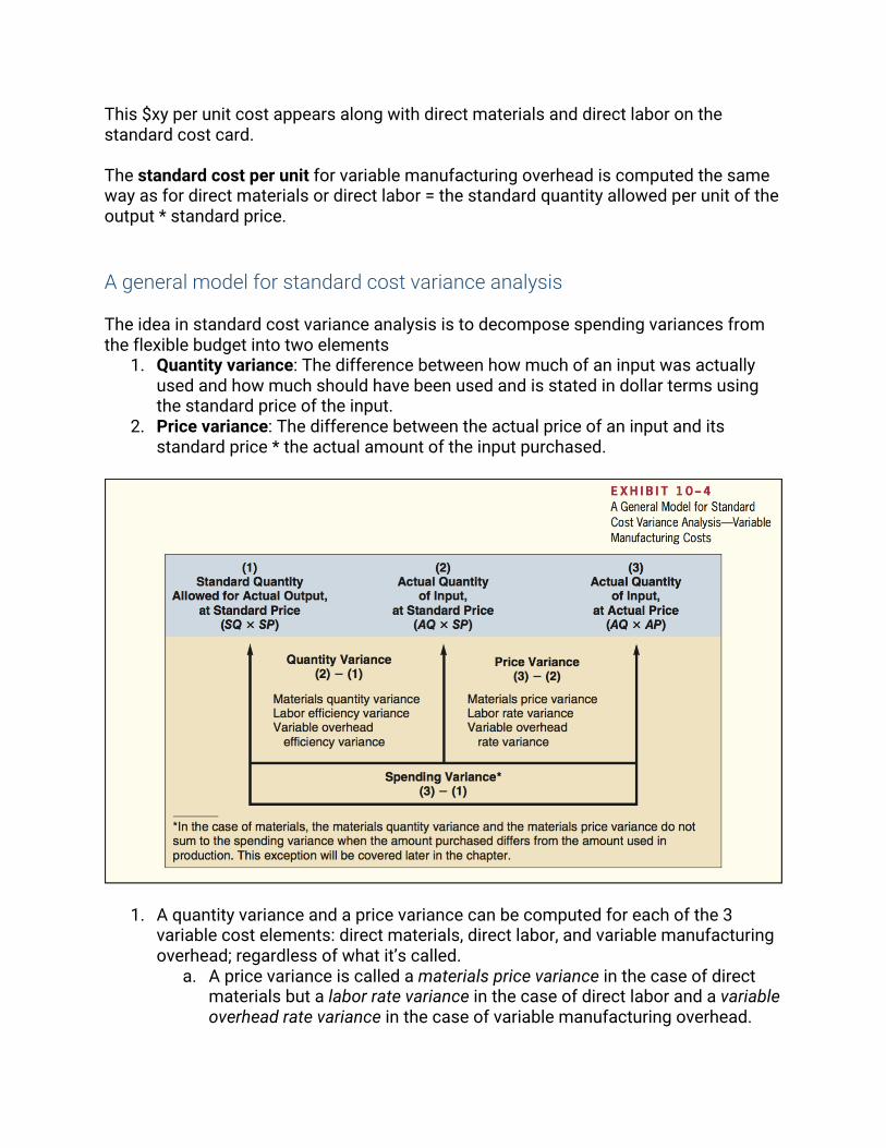
This $xy per unit cost appears along with direct materials and direct labor on the standard cost card. The standard cost per unit for variable manufacturing overhead is computed the same way as for direct materials or direct labor = the standard quantity allowed per unit of the output * standard price. A general model for standard cost variance analysis The idea in standard cost variance analysis is to decompose spending variances from the flexible budget into two elements

1. Quantity variance: The difference between how much of an input was actually used and how much should have been used and is stated in dollar terms using the standard price of the input.

2. Price variance: The difference between the actual price of an input and its standard price * the actual amount of the input purchased.

1. A quantity variance and a price variance can be computed for each of the 3 variable cost elements: direct materials, direct labor, and variable manufacturing overhead; regardless of what it’s called.

a. A price variance is called a materials price variance in the case of direct materials but a labor rate variance in the case of direct labor and a variable overhead rate variance in the case of variable manufacturing overhead.

2. The quantity variance, regardless of what it’s called, is computed in exactly the same way regardless of whether one is dealing with direct materials, direct labor, or variable manufacturing overhead. Same is true for price variance.

3. The input is the actual quantity of direct materials or direct labor purchased, the output is the good production of the period, expressed in terms of the standard quantity (or the standard hours) allowed for the actual output

The standard quantity allowed and standard hours allowed means the amount of an input that should’ve been used to produce the actual output of the period. Using standard costs – direct materials variances

A price or quantity variance is labeled unfavorable (U) if the actual purchase price or product used exceeds the standard. Materials quantity variance The materials quantity variance measures the difference between the quantity of materials used in production and the quantity that should have been used according to the standard. Generally used in dollar terms.

𝑀𝑎𝑡𝑒𝑟𝑖𝑎𝑙𝑠𝑞𝑢𝑎𝑛𝑡𝑖𝑡𝑦𝑣𝑎𝑟𝑖𝑎𝑛𝑐𝑒 = 𝐴𝑄 − 𝑆𝑄 𝑆𝑃 It is best to isolate the materials quantity variance when materials are used in production. Materials are drawn for the number of units to be produced, according to the standard bill of materials for each unit. Any additional materials are usually drawn with an excess materials requisition slip, which differs from the normal requisition slips. This procedure calls attention to the excessive usage of materials while production is still in process and provides an opportunity to correct any developing problem. Materials price variance A materials price variance measures the difference between what is paid for a given quantity of materials and what should have been paid according to the standard.

𝑀𝑎𝑡𝑒𝑟𝑖𝑎𝑙𝑠𝑝𝑟𝑖𝑐𝑒𝑣𝑎𝑟𝑖𝑎𝑛𝑐𝑒 = 𝐴𝑄(𝐴𝑃 − 𝑆𝑃) When using this formula, a negative variance is always labeled favorable and vice versa. Using standard costs – direct labor variances Labor efficiency variance The labor efficiency variance attempts to measure the productivity of direct labor.

𝐿𝑎𝑏𝑜𝑟𝑒𝑓𝑓𝑖𝑐𝑖𝑒𝑛𝑐𝑦𝑣𝑎𝑟𝑖𝑎𝑛𝑐𝑒 = 𝐴𝐻 − 𝑆𝐻 𝑆𝑅 Possible causes of an unfavorable labor efficiency variance include poorly trained or motivated workers; poor quality materials, requiring more labor time, faulty equipment,

poor supervision of workers, inaccurate standards. Another cause may be insufficient demand for the company’s products. Labor rate variance Labor rate variance: The price variance for direct labor.

𝐿𝑎𝑏𝑜𝑟𝑟𝑎𝑡𝑒𝑣𝑎𝑟𝑖𝑎𝑛𝑐𝑒 = 𝐴𝐻(𝐴𝑅 − 𝑆𝑅) Using standard costs – variable manufacturing overhead variances To compute the variable manufacturing overhead variances the variable portion of manufacturing overhead can be analyzed using the same basic formulas used to analyze direct materials and direct labor. Manufacturing overhead variances Variable overhead efficiency variances formula:

𝑉𝑎𝑟𝑖𝑎𝑏𝑙𝑒𝑜𝑣𝑒𝑟ℎ𝑒𝑎𝑑𝑒𝑓𝑓𝑖𝑐𝑖𝑒𝑛𝑐𝑦𝑣𝑎𝑟𝑖𝑎𝑛𝑐𝑒 = 𝐴𝐻 − 𝑆𝐻 𝑆𝑅

Variable overhead rate variance formula:

𝑉𝑎𝑟𝑖𝑎𝑏𝑙𝑒𝑜𝑣𝑒𝑟ℎ𝑒𝑎𝑑𝑟𝑎𝑡𝑒𝑣𝑎𝑟𝑖𝑎𝑛𝑐𝑒 = 𝐴𝐻(𝐴𝑅 − 𝑆𝑅)

An important subtlety in the materials variances Most companies compute the materials price variance when materials are purchased rather than when used in production for two reasons:

1. Delaying the computation of the price variance until the materials are used would result in less timely variance reports.

2. Computing the price variance when the materials are purchased allows materials to be carried in the inventory accounts at their standard cost, simplifying bookkeeping.

The equations presented earlier that define direct materials quantity and price variances are correct and reproduced below:

The materials quantity variance is based on the actual quantity used, whereas the materials price variance is based on the actual quantity purchased.

𝑀𝑎𝑡𝑒𝑟𝑖𝑎𝑙𝑠𝑞𝑢𝑎𝑛𝑡𝑖𝑡𝑦𝑣𝑎𝑟𝑖𝑎𝑛𝑐𝑒 = 𝐴𝑄𝑢𝑠𝑒𝑑 ∗ 𝑆𝑃 − (𝑆𝑄 ∗ 𝑆𝑃) 𝑀𝑎𝑡𝑒𝑟𝑖𝑎𝑙𝑠𝑝𝑟𝑖𝑐𝑒𝑣𝑎𝑟𝑖𝑎𝑛𝑐𝑒 = 𝐴𝑄𝑝𝑢𝑟𝑐ℎ𝑎𝑠𝑒𝑑 ∗ 𝐴𝑃 − (𝐴𝑄𝑝𝑢𝑟𝑐ℎ𝑎𝑠𝑒𝑑 ∗ 𝑆𝑃)

- 3 Can always be used to compute the direct materials variances. The computation of the quantity variance is based on the actual input used whereas the computation of the price variance is based on the amount of the input purchased. The price variance is computed on the entire amount of material purchased, whereas the quantity variance is computed only on the amount of materials used in production during the month. When these materials are used in future periods, a quantity variance will be computed. A price variance will not be computed when the materials are finally used because the price variance was computed when the materials were purchased. Because the quantity variance is based on the amount used whereas the price variance is based on the amount purchased, the two variances do not sum to the spending variance from the flexible budget, which is wholly based on the amount used.

Variance analysis and management by exception Variance analysis and performance reports are important elements of management by exception, which is an approach that emphasizes focusing on those areas of responsibility where goals and expectations are not being met.

The basic idea underlying a statistical control chart is that some random fluctuations in variances from period to period are normal. The rule of thumb in this company is to investigate all variances that are more than one standard deviation in either direction from zero. In addition to watching for unusually large variances, the pattern of the variances should be monitored. Evaluation of controls based on standard costs Advantages of standard costs

1. Standard costs are a key element in a management by exception approach. 2. Standard that are viewed as reasonable by employees can promote economy

and efficiency. 3. Standard costs can greatly simplify bookkeeping. 4. Standard costs fit naturally in an integrated system of responsibility accounting.

Potential problems with the use of standard costs

1. Standard cost variance reports are usually prepared on a monthly basis and often are released days or even weeks after the end of the month. As a consequence, the information in the report may be so outdated that it is almost useless.

2. If managers are insensitive and use variance reports as a club, morale may suffer.

3. Labor quantity standard and efficiency variances make two important assumptions.

a. They assume that the production process is labor-paced. b. The computations assume that labor is a variable cost

4. In some cases, a favorable variance can be as bad or worse than an unfavorable variance.

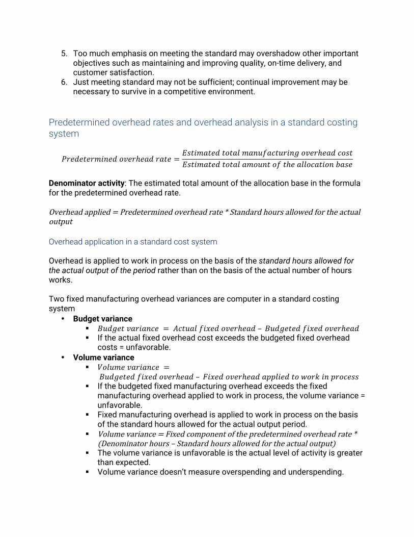
5. Too much emphasis on meeting the standard may overshadow other important objectives such as maintaining and improving quality, on-time delivery, and customer satisfaction.

6. Just meeting standard may not be sufficient; continual improvement may be necessary to survive in a competitive environment.

Predetermined overhead rates and overhead analysis in a standard costing system

𝑃𝑟𝑒𝑑𝑒𝑡𝑒𝑟𝑚𝑖𝑛𝑒𝑑𝑜𝑣𝑒𝑟ℎ𝑒𝑎𝑑𝑟𝑎𝑡𝑒 =𝐸𝑠𝑡𝑖𝑚𝑎𝑡𝑒𝑑𝑡𝑜𝑡𝑎𝑙𝑚𝑎𝑛𝑢𝑓𝑎𝑐𝑡𝑢𝑟𝑖𝑛𝑔𝑜𝑣𝑒𝑟ℎ𝑒𝑎𝑑𝑐𝑜𝑠𝑡𝐸𝑠𝑡𝑖𝑚𝑎𝑡𝑒𝑑𝑡𝑜𝑡𝑎𝑙𝑎𝑚𝑜𝑢𝑛𝑡𝑜𝑓𝑡ℎ𝑒𝑎𝑙𝑙𝑜𝑐𝑎𝑡𝑖𝑜𝑛𝑏𝑎𝑠𝑒

Denominator activity: The estimated total amount of the allocation base in the formula for the predetermined overhead rate. Overheadapplied=Predeterminedoverheadrate*Standardhoursallowedfortheactualoutput Overhead application in a standard cost system Overhead is applied to work in process on the basis of the standard hours allowed for the actual output of the period rather than on the basis of the actual number of hours works. Two fixed manufacturing overhead variances are computer in a standard costing system

• Budget variance § 𝐵𝑢𝑑𝑔𝑒𝑡𝑣𝑎𝑟𝑖𝑎𝑛𝑐𝑒 = 𝐴𝑐𝑡𝑢𝑎𝑙𝑓𝑖𝑥𝑒𝑑𝑜𝑣𝑒𝑟ℎ𝑒𝑎𝑑– 𝐵𝑢𝑑𝑔𝑒𝑡𝑒𝑑𝑓𝑖𝑥𝑒𝑑𝑜𝑣𝑒𝑟ℎ𝑒𝑎𝑑 § If the actual fixed overhead cost exceeds the budgeted fixed overhead

costs = unfavorable. • Volume variance

§ 𝑉𝑜𝑙𝑢𝑚𝑒𝑣𝑎𝑟𝑖𝑎𝑛𝑐𝑒 =𝐵𝑢𝑑𝑔𝑒𝑡𝑒𝑑𝑓𝑖𝑥𝑒𝑑𝑜𝑣𝑒𝑟ℎ𝑒𝑎𝑑– 𝐹𝑖𝑥𝑒𝑑𝑜𝑣𝑒𝑟ℎ𝑒𝑎𝑑𝑎𝑝𝑝𝑙𝑖𝑒𝑑𝑡𝑜𝑤𝑜𝑟𝑘𝑖𝑛𝑝𝑟𝑜𝑐𝑒𝑠𝑠

§ If the budgeted fixed manufacturing overhead exceeds the fixed manufacturing overhead applied to work in process, the volume variance = unfavorable.

§ Fixed manufacturing overhead is applied to work in process on the basis of the standard hours allowed for the actual output period.

§ Volumevariance=Fixedcomponentofthepredeterminedoverheadrate*(Denominatorhours–Standardhoursallowedfortheactualoutput)

§ The volume variance is unfavorable is the actual level of activity is greater than expected.

§ Volume variance doesn’t measure overspending and underspending.

Cautions in fixed overhead analysis A volume variance for fixed overhead arises because when applying the costs to work in process, we act as if the fixed costs are variable Fixed overhead costs come in large chunks. Expressing fixed costs on a unit or per hour basis, though necessary for product costing for external reports, is artificial. Increases or decreases in activity have no effect on total fixed costs within the relevant range of activity. Fixed costs are not proportional to activity. Reconciling overhead variances and underapplied or overapplied overhead In a standard cost system, the underapplied or overapplied overhead for a period = the sum of the overhead variance. Overhead is applied to work in process on the basis of the standard hours allowed for the actual output of the period.

𝑉𝑎𝑟𝑖𝑎𝑏𝑙𝑒𝑜𝑣𝑒𝑟ℎ𝑒𝑎𝑑𝑒𝑓𝑓𝑖𝑐𝑖𝑒𝑛𝑐𝑦𝑣𝑎𝑟𝑖𝑎𝑛𝑐𝑒 = (𝐴𝐻 ∗ 𝑆𝑅)–(𝑆𝐻 ∗ 𝑆𝑅)

𝑉𝑎𝑟𝑖𝑎𝑏𝑙𝑒𝑜𝑣𝑒𝑟ℎ𝑒𝑎𝑑𝑟𝑎𝑡𝑒𝑣𝑎𝑟𝑖𝑎𝑛𝑐𝑒 = (𝐴𝐻 ∗ 𝐴𝑅)–(𝐴𝐻 ∗ 𝑆𝑅) If the overhead is underapplied, the total of the standard cost overhead variances is unfavorable.

Capital budgeting decisions Capital budgeting is used to describe how managers plan significant investments in projects that have long-term implications such as the purchase of new equipment or the introduction of new products. Capital budgeting – planning investments Typical capital budgeting decisions include:

• Cost reduction decisions • Expansion decisions • Equipment selection decisions • Lease or buy decisions • Equipment replacement decisions

Capital budgeting decisions fall into two broad categories:

1. Screening decisions relate to whether a proposed project is acceptable 2. Preference decisions relate to selecting from among several acceptable

alternatives Capital investments usually earn returns that extend over fairly long periods of time, thus it’s important to recognize the time value of money when evaluating investment proposals. Projects that promise earlier returns are preferable to those that promise later returns. Capital budgeting techniques that recognize the time value of money involve discounting cash flows. Discounted cash flow – the net present value method Two approaches to making capital budgeting decisions use discounted cash flow:

1. Net present value a. Under the net present value method, the present value of a project’s cash

inflows is compared to the present value of the project’s cash outflows. The difference between the present value of these cash flows is the net present value, which determines whether or not the project is an acceptable investment

b. Deducting the present value of the required investment from the present value of the cost savings yields the net present value.

c.

d. 2. Internal rate of return

a. The rate of return of an investment project over its useful life. Discussed later.

Emphasis on cash flows Accounting net income is based on accruals that ignore when cash flows occur. In capital budgeting, the time of cash flows is critical. The present value of a cash flow depends on when it occurs. Cash flow rather than accounting net income is the focus in capital budgeting. 3 types of cash flows used by most projects:

• They often require an immediate cash outflow in the form of an initial investment in equipment, other assets, and installation costs.

• Some projects require a company to expand its workingcapital=currentassets–currentliabilities

• Many projects require periodic outlays for repairs and maintenance and additional operating costs.

Typical cash inflows 3 types of cash inflows used by most projects:

• A project will normally increase revenues or reduce costs. The amount involved should be treated as a cash inflow for capital budgeting purposes.

o From a cash flow standpoint, a reduction in costs is equivalent to an increase in revenues

• Cash inflows are also frequently realized from selling equipment for its salvage value when a project ends

• Any working capital that was tied up in the project can be released for use elsewhere at the end of the project and should be treated as a cash inflow at that time.

o E.g. Working capital is released when a company sells off its inventory or collects its accounts receivable.

Recovery of the original investment The net present value method automatically provides for return of the original investment. Whenever the net present value of a project is positive, the project will recover the original cost of the investment plus sufficient excess cash inflows to compensate the organization for tying up funds in the project. Simplifying assumptions 2 simplifying assumptions are usually made in net present value analysis:

1. All cash flows other than the initial investment occur at the end of periods. a. Somewhat unrealistic in that cash flows typically occur throughout a

period rather than just at its end. 2. All cash flows generated by an investment project are immediately reinvested at

a rate of return equal to the discount rate. Choosing a discount rate

• A positive net present value indicates that the project’s return exceeds the discount rate.

• A negative net present value indicates that the project’s return is less than the discount rate

If the company’s minimum required rate of return is used as the discount rate, a project with a positive net present value has a return that exceeds the minimum required rate of return and is acceptable. Cost of capital: Usually regarded as the minimum required rate of return, this is the average rate of return the company must pay to its long-term creditors and its shareholders for the use of their funds.

• If a project’s rate of return is less than the cost of capital, the company does not earn enough to compensate its creditors and shareholders.

• Cost of capital servers as a screening device. o When the cost of capital is used as the discount rate in net present value

analysis, any project with a negative present value does not cover the company’s cost of capital and should be discarded as unacceptable.

Out-of-pocket costs are actual cash outlays for salaries, advertising, and other operating expenses. Discounted cash flows – The internal rate of return method Internal rate of return: The rate of return of an investment project over its useful life. The internal rate of return is computed by finding the discount rates that equates the present value of a project’s cash outflows with the present value of its cash inflows. The internal rate of return is the discount rate that results in a net present value of zero. To compute the internal rate of return we must find the discount rate that will result in a zero net present value.

• Using the direct approach when the net cash inflow is the same every year by dividing the investment in the project by the expected annual net cash inflow. This yields a factor from which the internal rate of return can be determined. The formula:

• The factor derived from the formula is then located in the present value tables to see what rate of return it represents.

𝐹𝑎𝑐𝑡𝑜𝑟𝑜𝑓𝑡ℎ𝑒𝑖𝑛𝑡𝑒𝑟𝑛𝑎𝑙𝑟𝑎𝑡𝑒𝑜𝑓𝑟𝑒𝑡𝑢𝑟𝑛 =𝐼𝑛𝑣𝑒𝑠𝑡𝑚𝑒𝑛𝑡𝑟𝑒𝑞𝑢𝑖𝑟𝑒𝑑𝐴𝑛𝑛𝑢𝑎𝑙𝑛𝑒𝑡𝑐𝑎𝑠ℎ𝑖𝑛𝑓𝑙𝑜𝑤

Salvage value and other cash flows If a project’s cash flows are not identical every year a trial-and-error process may be used to find the rate of return that will result in a zero net present value. Using the internal rate of return

To evaluate a project, the internal rate of return is compared to the company’s minimum required rate of return, usually the company’s cost of capital. If the internal rate of return is equal to or greater than the required rate of return, the project is acceptable. The cost of capital as a screening tool

• Cost of capital is often used to screen out undesirable investment projects. • When the internal rate of return method is used, the cost of capital is used as the

hurdle rate that a project must clear for acceptance. • When the net present value method is used, the cost of capital is the discount

rate used to compute the net present value of a proposed project. Comparison of the net present value and internal rate of return methods Net present value method has several advantages over the internal rate of return method:

• The net present value method is often simpler to use than the internal rate of return method.

• The internal rate of return method makes a questionable assumption. o Both methods assume that cash flows generated by a project during its

useful life are immediately reinvested elsewhere. o The two methods make different assumptions concerning the rate of

return that is earned on those cash flows. o The net present value method assumed the rate of return is the discount

rate, the internal rate of return method assumes the rate of return earned on cash flows is the internal rate of return on the project.

o If the internal rate of return of the project is high, this assumption may not be realistic.

o It is more realistic to assume that cash inflows can be reinvested at a rate of return equal to the discount rate, particularly if the discount rate is the company’s cost of capital or an opportunity rate of return.

• When the net present value method and the internal rate of return method do not agree concerning the attractiveness of a project, it’s best to go with the net present value method.

Expanding the net present value method Two approached to compare competing investment projects

1. The total cost approach 2. The incremental cost approach

The total-cost approach The total-cost approach is the most flexible method for comparing competing projects.

• All cash inflows and all cash outflows are included in the solutions under each alternative.

• A net present value is computed for each alternative. This is a distinct advantage of the total-cost approach because an unlimited number of alternatives can be compared side by side to determine the best option.

The incremental-cost approach When only two alternatives are being considered, the incremental-cost approach offers a simpler and more direct route to a decision.

• In the incremental-cost approach, only those costs and revenues that differ between the two alternatives are included in the analysis.

Least-cost decisions Some decisions do not involve any revenue. In situations such as these, the most desirable alternative is the one with the least total cost from a present value perspective. These are known as least-cost decisions. Uncertain cash flow Postponement is a particularly attractive option when the net present value of a project is modest using current estimates of future cash flows and the future cash flows involve a great deal of uncertainty that may be resolved over time. Once an investment is made, management can often exploit changes in the business environment and take actions that enhance future cash flows. Preference decisions – the ranking of investment projects When considering investment opportunities, managers must make 2 types of decisions:

1. Screening decisions: a. Come first. b. Pertain to whether or not a proposed investment is acceptable.

2. Preference decisions: a. Come after screening decisions. b. Attempt to answer the following question: How do the remaining

investment proposals rank in terms of preference? c. Sometimes called rationing decisions or ranking decisions.

Either the internal rate of return method or the net present value method can be used in making preference decisions. Net present value method is more reliable.

Internal rate of return method The higher the internal rate of return, the more desirable the project. Internal rate of return is widely used to rank projects. Net present value method The net present value of one project cannot be directly compared to the net present value of another project unless the initial investments are equal. Project profitability index: When different projects have an equal net present value but are not equally desirable they can be highlighted by this formula:

𝑃𝑟𝑜𝑗𝑒𝑐𝑡𝑝𝑟𝑜𝑓𝑖𝑡𝑎𝑏𝑖𝑙𝑖𝑡𝑦𝑖𝑛𝑑𝑒𝑥 =𝑁𝑒𝑡𝑝𝑟𝑒𝑠𝑒𝑛𝑡𝑣𝑎𝑙𝑢𝑒𝑜𝑓𝑡ℎ𝑒𝑝𝑟𝑜𝑗𝑒𝑐𝑡

𝐼𝑛𝑣𝑒𝑠𝑡𝑚𝑒𝑛𝑡𝑟𝑒𝑞𝑢𝑖𝑟𝑒𝑑

The higher the project profitability index, the more desirable the project. Other approaches to capital budgeting decisions The net present value and internal rate of return methods are widely used as decisions making tools. Another tool for making capital budgeting decisions is the payback method. The payback method The payback method focuses on the payback period. Payback period: The length of time that it takes for a project to recover its initial cost from the net cash inflows that it generates.

• Sometimes referred to as the time that it takes for an investment to pay for itself. • The quicker the cost of an investment can be recovered, the more desirable the

investment. • Payback period is expressed in years. • When the annual net cash inflow is the same every year we can use this formula:

o 𝑃𝑎𝑦𝑏𝑎𝑐𝑘𝑝𝑒𝑟𝑖𝑜𝑑 = �����~���~����������������~��������}�

Evaluation of the payback method

• The payback method is not a true measure of the profitability of an investment, it simply tells a manager how many years are required to recover the original investment.

• The payback method ignores all cash flows that occur after the payback period.

• It does not consider the time value of money. The payback method can be useful if used as a screening tool to help answer the question: Should I consider this proposal further? It is often important to new companies that are cash poor, and it is also sometimes used in industries where products become obsolete rapidly. An extended example of payback If new equipment is replacing old equipment, then any salvage value to be received when disposing of the old equipment should be deducted from the cost of the new equipment, and only the incremental investment should be used in the payback computation. In addition, any depreciation deducted in arriving at the project’s net operating income must be added back to obtain the project’s expected annual net cash inflow.

1. Depreciation is added back to net operating income to obtain the annual net cash inflow from the new equipment. Depreciation is not a cash outlay; thus, it must be added back to adjust net operating income to a cash basis.

2. The payback computation deducts the salvage value of the old machines from the cost of the new equipment so that only the incremental investment is used in computer the payback period.

Payback and uneven cash flows When the cash flows associated with an investment project change from year to year, simple payback formula outlined earlier can not be used. The simple rate of return method Simple rate of return method is another capital budgeting technique that doesn’t involve discounting cash flows. Also known as the accounting rate of return or the adjusted rate of return. The simple rate of return method focuses on accounting net operating income rather than cash flows:

𝑆𝑖𝑚𝑝𝑙𝑒𝑟𝑎𝑡𝑒𝑜𝑓𝑟𝑒𝑡𝑢𝑟𝑛 =𝐴𝑛𝑛𝑢𝑎𝑙𝑖𝑛𝑐𝑟𝑒𝑚𝑒𝑛𝑡𝑎𝑙𝑛𝑒𝑡𝑜𝑝𝑒𝑟𝑎𝑡𝑖𝑛𝑔𝑖𝑛𝑐𝑜𝑚𝑒

𝐼𝑛𝑖𝑡𝑖𝑎𝑙𝑖𝑛𝑣𝑒𝑠𝑚𝑒𝑛𝑡

1. Depreciation charges that result from making the investment should be deducted when determining the annual incremental net operating income.

2. The initial investment should be reduced by any salvage value realized from the sale of old equipment.

The simple rate of return method ignores the time value of money.

Postaudit of investment projects Postaudit: involves checking whether or not expected results are actually realized.

• Any tendency to inflate the benefits or downplay the costs should become evident.

• Also provides ab opportunity to reinforce and possibly expand successful project and to cut losses on floundering projects.

• The same capital budgeting method should be used in the postaudit as was used in the original approval process.

• The data used in the postaudit analysis should be actual observer data rather than estimated data.

The concept of present value A dollar received today is more valuable than a dollar received a year from now. Mathematics of interest

𝐹� = 𝑃(1 + 𝑟) F1 = the balance at the end of the period P= the amount invested now (present value or discounted value of the future $x) r= the rate of interest per period Compound interest: Interest can be compounded on a semiannual, quarterly, monthly, or even more frequent basis.

𝐹� = 𝑃(1 + 𝑟)� n= the number of periods of compounding Computation of present value An investment can be viewed in 2 ways:

1. In terms of future value 2. In terms of present value

The present value of any sum to be received in the future can be computer by:

𝑃 =𝐹�

(1 + 𝑟)�

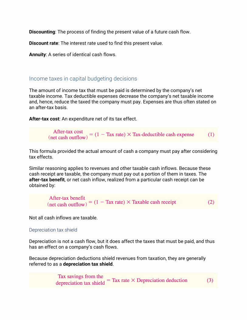
Discounting: The process of finding the present value of a future cash flow. Discount rate: The interest rate used to find this present value. Annuity: A series of identical cash flows. Income taxes in capital budgeting decisions The amount of income tax that must be paid is determined by the company’s net taxable income. Tax deductible expenses decrease the company’s net taxable income and, hence, reduce the taxed the company must pay. Expenses are thus often stated on an after-tax basis. After-tax cost: An expenditure net of its tax effect.

This formula provided the actual amount of cash a company must pay after considering tax effects. Similar reasoning applies to revenues and other taxable cash inflows. Because these cash receipt are taxable, the company must pay out a portion of them in taxes. The after-tax benefit, or net cash inflow, realized from a particular cash receipt can be obtained by:

Not all cash inflows are taxable. Depreciation tax shield Depreciation is not a cash flow, but it does affect the taxes that must be paid, and thus has an effect on a company’s cash flows. Because depreciation deductions shield revenues from taxation, they are generally referred to as a depreciation tax shield.

Because the net book value of the asset at the end of its useful life will be zero under this depreciation method, we will assume that any proceeds received on disposal of the asset at the end of its useful life will be taxed as ordinary income. In actuality, the rules for depreciation are more complex than this and most companies take advantage of accelerated depreciation methods allowed under the tax code. These accelerated methods usually result in a reduction in current taxes and an offsetting increase in future taxes.

Example of income taxes and capital budgeting ---Example of pages 634 and 635---