Accounting Earnings and Free Cash Flow

Peter Easton

Center for Accounting Research and Education

University of Notre Dame

Peter Vassallo

Adelaide Business School

University of Adelaide

Eric Weisbrod

School of Business Administration

University of Miami

January 2017

We thank Ryan Ball, Bill Beaver, Sanjay Bissessur, Khrystyna Bochkay, Demetris Christodoulou, Dan Collins, Mincherng Deng, Joseph Gerakos, Aloke Ghosh, Stephan Hollander, Jereon Suijs, Adel Ibrahim, Chris Jones, Zach Kaplan, Sok-Hyon Kang, Yaniv Konchitchki, Bin Li, Stephannie Larocque, Steve Lilien, David Lont, Martein Lubberink, Steve Monahan, Jim Ohlson, Suresh Radhakrishnan, Sundaresh Ramnath, Oded Rosenbaum, Alain Schatt, Mike Minnis, Pervin Shroff, Greg Sommers, Theodore Sougiannis, Ulrike Thurheimer, Michael Turner, Oktay Urcan, Clare Wang (discussant), Terry Walter, Bill Wright, Nir Yehuda, Xiao-Jun Zhang, and seminar participants at Baruch College, George Washington University, INSEAD Accounting Symposium - Singapore, Lausanne HEC, Shanghai Advanced Institute of Finance, Southern Methodist University, Tilburg University, MEAFA Conference, University of Adelaide, University of Amsterdam, University of Auckland, University of California at Berkeley, Erasmus University of Rotterdam, University of Illinois at Urbana-Champaign, University of Illinois at Chicago, University of Miami, University of Michigan, University of Otago, University of Queensland, University of Sydney, University of Texas at Dallas, Victoria University of Wellington and participants in the Washington University conference to honor Nick Dopuch, for helpful comments on an earlier draft.

Accounting Earnings and Free Cash Flow

Abstract

The extant literature has focused on the relation between earnings and returns (i.e., change in value). Yet change in firm value arises from two sources: (1) return on the assets in place; and, (2) cash flows to/from debt holders, equity holders, and/or cash reserves (i.e., free cash flow). The primary contribution of our paper is to add analysis of the relation between earnings and free cash flow. We show that: (1) free cash flow explains more of operating income than is explained by returns; (2) the difference in the portion of negative cf. positive enterprise returns captured in operating income is similar to the portion of negative cf. positive equity returns captured in earnings reported in the extant literature and this portion is different if there is net cash inflow vs. net cash outflow; (3) the portion of each source of change in value captured in operating income changes with leverage, thus, we extend the extant literature on the effect of leverage on “conservative” accounting; (4) leverage varies with type of investment and, since the accounting varies with the type of investment, the portions of change in value captured in operating income varies, thus, we provide an alternative explanation for the relation between leverage and the degree of conservatism in accounting.

Keywords: Firm Growth, Free Cash Flows, Earnings Return Relation, NOPAT, Valuation

1

I. Introduction

Operating income, which is the accounting measure of change in value of the firm, captures

a portion of this change in value and this portion depends on the source of change in value.1

Change in firm value arises from two sources:

(1) investment (and disinvestment) of cash by the firm’s capital providers (i.e., debt and

equity holders); we argue and show that the portion of free cash flow that is captured in

operating income reflects accounting rules, which require expensing of the investment rather

than capitalizing into book value.2 Importantly, this expensing results in a reduction in

operating income even though the free cash flow per se does not change profitability,3and,

(2) change in the value of the firm’s operating assets, which reflects change in profitability

of the current period and change in expectations of future profitability; only the former

portion is captured in concurrent operating income.

The analyses in the extant literature, which has examined the portion of equity returns that is

captured in earnings, is quite similar to our analyses of the portion of firm-level returns that is

captured in operating income. The extant literature has not, however, recognized the fact that

operating income (and earnings) is also affected by the accounting for the other source of change

1 The method of calculation of operating income, which is the income from the enterprise operations of the firm is shown in the Appendix. Operating income is sometimes referred to as net operating profit after tax (NOPAT).

2 Free cash flow is the operating income of the firm in excess of the investment in maintaining or expanding the enterprise assets. This free cash flow goes to equity holders (in the form of dividends and stock repurchases), to debt holders (in the form of interest payments and debt repayments) and to build up cash reserves. Of course, free cash flow will be negative if growth in operating assets is greater than operating profits. The method of calculation of free cash flow is shown in the Appendix.

3 After the cash is invested in the firm, it, of course, becomes part of the assets in the firm and may affect both current and future profitability.

2

in value – free cash flow. We show that growth through free cash flow explains as much of

cross-sectional variation in operating income as is explained by returns and that the accounting

for this growth in operating income identifies, conceptually and empirically, distinct forms of

accounting for firm level change in value. Also, we predict and show that the portion of returns

that is captured in concurrent operating income depends on the sign of both returns and free cash

flow. In doing so, we provide a significant new dimension to the vast literature on the relation

between earnings and returns.

In order to illustrate the importance of: (1) focusing on operating income and firm returns

rather than earnings and equity returns as in the extant literature; and, (2) adding free cash flow

to the earnings/return regression, we also partition our sample on the debt/equity ratio and show

how the type of firm assets differs across these partitions and, in turn, the accounting (i.e., the

portion of return and free cash flow that is captured in operating income) differs. An implication

of our results is that conclusions in the extant literature regarding the influence of debt/equity

ownership on the earnings/returns relation may reflect no more than differences in the

accounting for different assets (e.g., full expensing of investment in R&D, which tends to be the

primary form of investment when the firm is mostly owned by equity holders vs. capitalizing

investment in property, plant and equipment, which tends to be the primary form of investment

when the firm is owned by debt holders).

A vast literature, starting with Ball and Brown (1967, 1968), has examined the relation

between earnings and change in value of existing investments. The more recent literature,

particularly since Basu (1997), argues and shows that the portion of decrease in the market value

of existing assets that is captured in concurrent earnings is greater than the portion of increase in

value that is captured in concurrent earnings. The extant literature has not analyzed the relation

3

between earnings and the change in value due to the provision of new capital (that is cash flow).

This analysis is the primary contribution of our paper.

We ask two questions regarding the relation between operating income and the two sources

of change in value. First, how and why does the portion of change in value that is captured in

concurrent operating income differ across the two sources of change in value? Second, how and

why does the interaction between these two sources of change in firm value affect the portion of

the change in firm value that is captured in concurrent operating income?

We argue, for example, that capital providers will tend to provide cash to the firm when they

think that negative returns are due to shorter run issues but they will tend to remove cash when

the negative returns reflect more permanent changes. It follows that, when there is cash inflow

to the firm, the portion of negative returns that is captured in concurrent operating income will be

greater than when there is cash outflow.

Further, we ask: how does the portion of change in firm value that is captured in concurrent

operating income change with firm leverage? How does this portion differ across the two sources

of change in value? How does the type of assets in which the firm invests affect these portions?

We show that leverage varies with type of investment (capital intensive firms tend to have higher

leverage than R&D intensive firms) and, since the accounting varies with the type of investment,

the portions of change in value captured in concurrent operating income vary with leverage and

investment type.

How and why do the portions of change in value that is captured in concurrent earnings vary

with the source and sign of the change in value? We begin by providing short answers to this

4

question for each of the sources of change in value and for increase and decrease in firm value

arising from these sources.

The portion of the change in value arising from cash flow from capital providers (i.e., cash

inflow), which is recorded in operating income, varies from zero to one depending on the type of

investment. If the investment is in R&D, generally, all of the cash investment will be expensed

in operating income. If the investment is in property, plant and equipment the only effect on

operating income for the fiscal period will be the depreciation of the asset over the rest of the

fiscal period with the remaining effect of the cash flow being recorded as an increase in book

value; if there is no depreciation, none of the cash investment will be expensed in operating

income.

The portion of the change in value arising when there is cash flow to capital providers (i.e.,

cash outflow), which is recorded in operating income, also varies with the type of investment.

To illustrate, compare a firm that is R&D intensive and a firm that is capital intensive. R&D

firms must generate cash outflow from the operating income of the current period; i.e., all of the

cash outflow will arise from current operating income. But, a firm that is capital intensive may

sell assets to generate cash outflow. If all of the cash outflow is generated by the asset sales and

the book value of these assets is the same as the market value none of the cash outflow will be

associated with operating income of the period. On the other hand, if the book value of the

assets is zero, there will be a “gain on sale” recorded in operating income; all of the cash outflow

will be recorded in operating income.

The portion of the change in the market value of existing operating assets, which is captured

in concurrent earnings, will reflect the portion that arises from earnings of the current period

5

rather than from changes in expectations of earnings of future periods. This portion will,

generally, range from zero, if all of the change in value is due to change in expected future

earnings, to one, if all of the change in value is due to earnings of the current period. Accounting

for the change in value of equity returns has received much attention in the recent literature,

which focuses on the difference in the portion of positive equity returns that is captured in

current earnings vis-à-vis the portion of negative equity returns that is captured in current

earnings (e.g., Basu 1997). We show similar results when we examine the portion of positive vs.

negative enterprise returns that is captured in operating (enterprise) income.4 We predict and

show, however, that these portions (of both positive and negative returns) differ considerably

between samples where the owners are injecting further cash into the enterprise (implicitly they

are confident in their expectations regarding future growth) and samples where cash is being

removed (implicitly the owners are removing cash and investing it elsewhere).5

Our analyses are based on a multiple regression of operating income on contemporaneous

returns and free cash flow. The estimates of the coefficients on returns and free cash flow capture

4 We use the term enterprise to describe the entity (sometimes called the firm) that is jointly owned by the capital providers (i.e., the debt and equity holders). Enterprise return is the sum of the change in the market value of equity, the change in the market value of debt, and cash flows (in the form of dividends payments, interest payments, proceeds from new stock issues and new debt, etc.) to/from the capital providers.

5 There are two reasons for our focus on the enterprise rather than on the equity ownership of the enterprise, as in most of the extant literature. First, the book value of financial assets and financial liabilities is generally close to the market value of these financial assets and financial liabilities but the book value of enterprise assets usually is much less than the market value of these assets; and the accounting for enterprise revenue and expenses is likely to be less than dollar-for-dollar, while the accounting for interest income and expenses is, as a first approximation, dollar-for-dollar. In short, analyses at the enterprise level focus on the entity where the mapping from change in value to accounting numbers is not simply dollar-for-dollar. In contrast, analyses of accounting at the equity level is based on earnings that are a combination of enterprise earnings, which are accounted for conservatively, and financial expenses, which are not accounted for conservatively. Second, when the enterprise is the entity of interest, cash contributions/distributions come from/go to the owners of the enterprise (viz., debt and equity holders) in to/out of the enterprise. On the other hand, dividends and stock repurchases may be funded from cash reserves (financial assets) or extra debt (financial liabilities); in other words, dividends may represent transactions between the owners of the enterprise and there is no conservatism in the accounting for these transactions.

6

the portion of these sources of change in value captured in contemporaneous earnings. Although

the effect on operating income (earnings) of firm growth (change in value) due to

investment/disinvestment of cash by the capital providers has received little attention in the

extant literature, we show that it explains at least as much of operating income as is explained by

returns, and in some cases more.6 In essence, we show that accounting measures of firm value

change are often more strongly associated with value change arising from transactions between

the firm and its capital providers during the period than with returns of the period.

In short, we argue and show that: (1) the accounting for growth (i.e., value change) differs

according to the source of the growth; (2) free cash flows to/from the capital providers to the

enterprise explain at least as much of the cross-sectional variation in operating income as is

explained by returns on assets in place; and, (3) the portion of returns and the portion of free cash

flow that is captured in concurrent operating income differ according to the sign of returns (i.e.,

whether the assets in place are increasing or decreasing in value) and according to the sign of

free cash flow (i.e., whether the capital providers to the firm are providing more cash or

removing cash).7

6 Our analysis of free cash flow departs from the extant literature that considers the mapping from changes in value to cash flows rather than the mapping from cash flows to earnings (e.g., Collins, Hribar, and Tian 2014, who examine the mapping from equity returns to operating cash flows, and Penman and Yehuda 2004, who examine the mapping from free cash flows to change in enterprise value). As far as we are aware, the mapping from FCF to OI, which explains much of the cross-sectional variation in operating income, has not yet been considered in the literature on accounting for value change.

7 Unreported analyses show that the coefficient relating equity earnings to equity returns also differs considerably from the coefficient relating earnings to net transactions with equity holders (i.e., “dividends”) and that “dividends” has significant incremental explanatory power for earnings over returns. We do not report these results because (as we have argued in footnote 5) these results reflect a mixture of accounting for the enterprise, which tends to be conservative, and accounting for debt, which tends not to be conservative.

7

The remainder of the paper proceeds as follows. We begin, in Section II by presenting our

motivation and the empirical model. In doing so, we demonstrate our reasons for our focus on

accounting at the enterprise level and for the addition of free cash flow. We present our

predictions in Section III. We describe our sample selection procedure in Section IV, and

discuss selected descriptive statistics. Section V analyzes and compares partitions of the data

based on whether enterprise value is increasing or decreasing and on the source of this value

increase/decrease. In Section VI, we examine whether the empirical manifestation of change in

enterprise value in the financial statements differs as expected with change in leverage and

enterprise asset types. Section VII presents a summary and conclusions.

II. Motivation and Model Development

There are two sources of change in the market value of the firm and the accounting (and

hence the portion of change in value that is captured in operating income) differs across these

two sources. The two sources are: (1) returns on existing assets and on new investments; and,

(2) transactions with capital providers (i.e., free cash flow).8 We will discuss the accounting for

each source of change in the market value of the firm separately, beginning with (1), which is the

focus of prior literature on the accounting for change in equity value.

The question at the heart of the empirical literature, which considers accounting

measurement of value and change in value is: what portion of equity returns is captured in

8 While the term free cash flow contains the word “cash,” FCF inflows and outflows include all forms of value flowing between the enterprise and the owners of the enterprise. For example, FCF includes contributions from the owners of an acquired company where the acquisition currency is shares in the newly-formed enterprise (e.g., the 2006 acquisition of Gillette by Procter and Gamble).

8

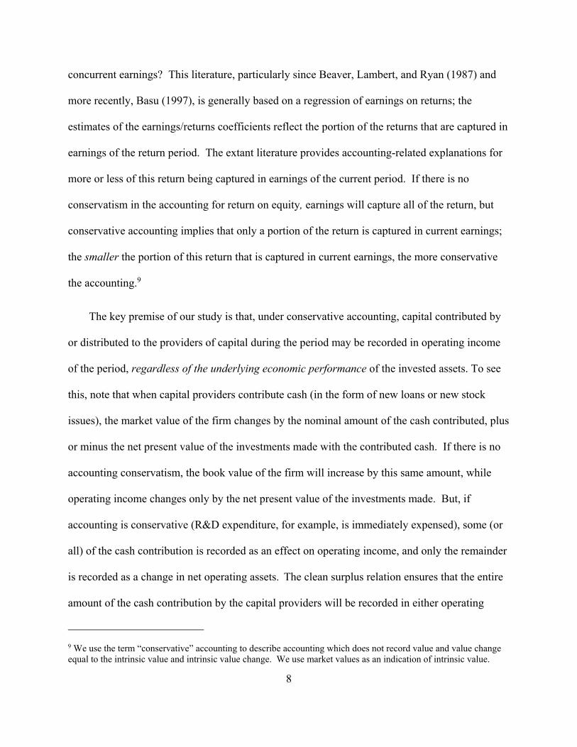
concurrent earnings? This literature, particularly since Beaver, Lambert, and Ryan (1987) and

more recently, Basu (1997), is generally based on a regression of earnings on returns; the

estimates of the earnings/returns coefficients reflect the portion of the returns that are captured in

earnings of the return period. The extant literature provides accounting-related explanations for

more or less of this return being captured in earnings of the current period. If there is no

conservatism in the accounting for return on equity, earnings will capture all of the return, but

conservative accounting implies that only a portion of the return is captured in current earnings;

the smaller the portion of this return that is captured in current earnings, the more conservative

the accounting.9

The key premise of our study is that, under conservative accounting, capital contributed by

or distributed to the providers of capital during the period may be recorded in operating income

of the period, regardless of the underlying economic performance of the invested assets. To see

this, note that when capital providers contribute cash (in the form of new loans or new stock

issues), the market value of the firm changes by the nominal amount of the cash contributed, plus

or minus the net present value of the investments made with the contributed cash. If there is no

accounting conservatism, the book value of the firm will increase by this same amount, while

operating income changes only by the net present value of the investments made. But, if

accounting is conservative (R&D expenditure, for example, is immediately expensed), some (or

all) of the cash contribution is recorded as an effect on operating income, and only the remainder

is recorded as a change in net operating assets. The clean surplus relation ensures that the entire

amount of the cash contribution by the capital providers will be recorded in either operating

9 We use the term “conservative” accounting to describe accounting which does not record value and value change equal to the intrinsic value and intrinsic value change. We use market values as an indication of intrinsic value.

9

income (as an expense) or in net operating assets (as an asset); the more conservative the

accounting, the greater the portion of the cash contribution that is captured in concurrent

operating income.

Similarly, when there is a payment to the capital providers (in the form of dividends, stock

repurchases, interest and/or loan repayments) and there is no conservatism, the book value of the

firm (net operating assets) decreases by the cash payment and there is no effect on operating

income. But, if accounting is conservative, the decrease in the book value of net operating assets

(i.e., NOA) associated with the cash payment will be understated, and, as a result, operating

income (i.e., OI) will be overstated, relative to the no conservatism case. For example, if the

depreciated value of assets sold to generate the cash payment is less than the sale value, NOA

will decrease by the book value of the sold asset, but the remainder of the cash flow will be

recorded in OI as a gain on sale. Again, the clean surplus relation ensures that the entire amount

of the cash distribution to the capital providers will be recorded in either OI or in ΔNOA (as a

decline in asset value); and, again, the more conservative the accounting, the greater the portion

of the cash distribution that is captured in current OI.

Furthermore, under conservative accounting, the association between OI and FCF will occur

in the same period as FCF, even if the investment of the FCF is transaction is zero-NPV or the

economic performance that generates the expense or gain on sale was recognized in market value

in a different period. We continue the asset sale example to illustrate this point. Increases in the

market value of an asset in prior periods would have been captured in the returns of those prior

periods, but the gain on sale will be captured in OI during the period in which the asset is

liquidated (i.e., the period in which the cash payment is made to the capital providers).

10

The key point of this discussion is that the accounting for growth due to the provision of

cash (i.e., FCF) may lead to an association between FCF and OI of the period, independent of

current period returns; this suggests that we may gain additional insights if we add FCF to the

regression of operating income on returns:

it = β0t+β1t +β2t

ε1it (1)

where it is the operating income of firm i for year t, it is the market value of the firm

(enterprise operations) of firm i at time t, is the returns on the firm for the period

ending at t, and it is free cash flow to/from the providers of capital to the firm (i.e., equity

and net debt holders). Henceforth, for ease of exposition, we also drop subscripts and

denominators when referring to the measures of OI and FCF used in our analyses.10

III. Empirical Predictions

Most of our empirical analyses are based on regression (1). In the absence of conservatism,

OI = ΔEV + FCF and it follows that the estimates of the coefficient relating OI to RETent would

be one and the coefficient relating OI to FCF would be zero. We show, however, that, in the

presence of conservatism, the estimates of the coefficients differ from these baselines of one and

zero in predictable ways, according to the signs of RETent and FCF. The two coefficients capture

distinct aspects of accounting, with more conservative accounting generating smaller coefficients

(i.e., less than one) on RETent and larger coefficients (i.e., greater than zero) on FCF.

10 Easton (2016) provides a detailed discussion of the relations between regression (1) at the equity level and regression (1) at the enterprise level.

11

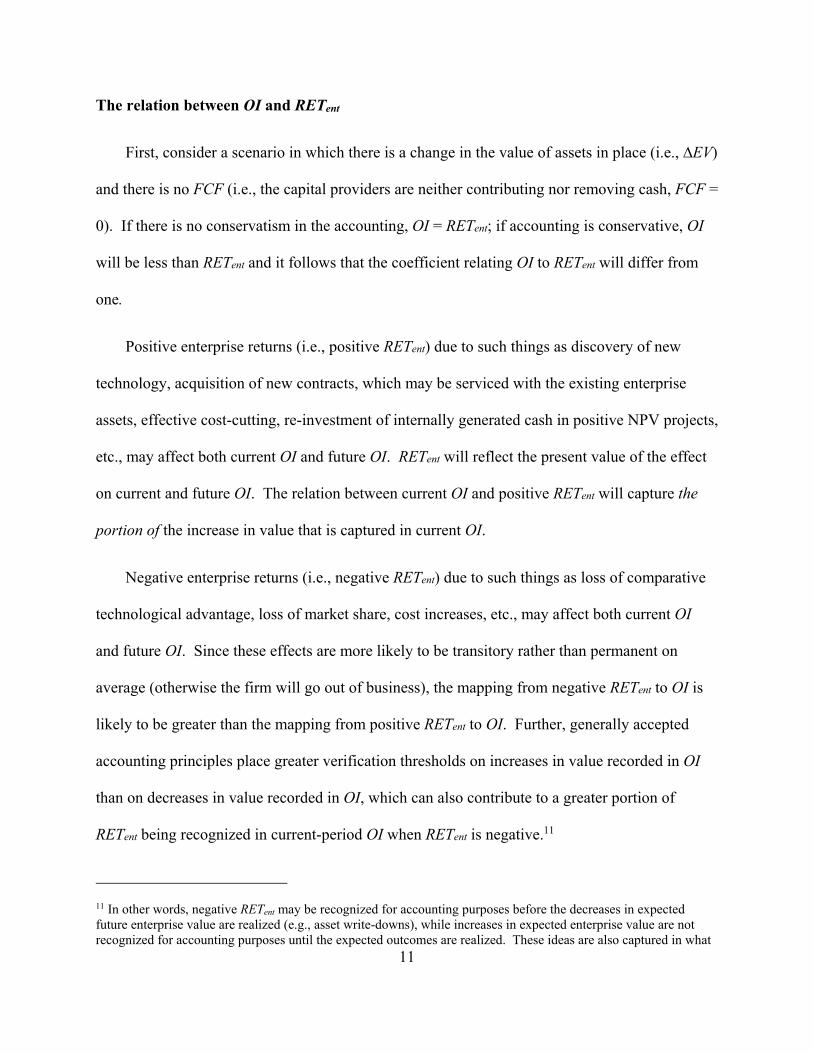
The relation between OI and RETent

First, consider a scenario in which there is a change in the value of assets in place (i.e., ∆EV)

and there is no FCF (i.e., the capital providers are neither contributing nor removing cash, FCF =

0). If there is no conservatism in the accounting, OI = RETent; if accounting is conservative, OI

will be less than RETent and it follows that the coefficient relating OI to RETent will differ from

one.

Positive enterprise returns (i.e., positive RETent) due to such things as discovery of new

technology, acquisition of new contracts, which may be serviced with the existing enterprise

assets, effective cost-cutting, re-investment of internally generated cash in positive NPV projects,

etc., may affect both current OI and future OI. RETent will reflect the present value of the effect

on current and future OI. The relation between current OI and positive RETent will capture the

portion of the increase in value that is captured in current OI.

Negative enterprise returns (i.e., negative RETent) due to such things as loss of comparative

technological advantage, loss of market share, cost increases, etc., may affect both current OI

and future OI. Since these effects are more likely to be transitory rather than permanent on

average (otherwise the firm will go out of business), the mapping from negative RETent to OI is

likely to be greater than the mapping from positive RETent to OI. Further, generally accepted

accounting principles place greater verification thresholds on increases in value recorded in OI

than on decreases in value recorded in OI, which can also contribute to a greater portion of

RETent being recognized in current-period OI when RETent is negative.11

11 In other words, negative RETent may be recognized for accounting purposes before the decreases in expected future enterprise value are realized (e.g., asset write-downs), while increases in expected enterprise value are not recognized for accounting purposes until the expected outcomes are realized. These ideas are also captured in what

12

The relation between OI and FCF

If there is no conservatism in the accounting, OI = RETent, and the coefficient relating OI to

FCF would be zero. When FCF is negative, indicating that the capital providers are contributing

cash to the firm and there is no conservatism in the accounting for the associated investment,

∆NOA = - FCF plus the NPV of the investment. The NPV of the FCF investment will be part of

RETent and like other sources of RETent only the portion of the NPV that is related to current

change in profit will be recorded in OI. But, if mandatory accounting rules require conservative

expensing of FCF investments, (R&D expenditure, for example, is immediately expensed), some

(or all, if the expenditure is on R&D) of the nominal amount of FCF will be captured in OI

(regardless of the NPV of the investment); the more conservative the accounting, the greater the

portion of the FCF that is captured in OI.

Similarly, if FCF is positive and there is no conservatism, ∆NOA = - FCF and there is no

OI. But, if accounting is conservative (e.g., the depreciated value of assets sold to generate the

cash is less than the sale value), NOA will decrease by the book value of the sold asset and

remainder of the FCF will be recorded as a gain on sale in OI. Again, the more conservative the

accounting, the greater the portion of change in firm value due to FCF that is captured in current

OI. The accumulated effects of accounting from the past will lead to lower recorded asset value

(i.e., the “gain on sale”, which will be recorded in operating income, increases, ceteris paribus,

with accounting conservatism) as well as lower expenses matched to sales of the period

Roychowdhury and Watts (2007) refer to as “rents” and Ball, Kothari and Nikolaev (2013) label as the g component of stock returns (which is associated with “revisions in the value of growth options or un-booked intangibles”), as well as “curtailment”, which is the focus of Lawrence et al. (2015). Returns may also be generated from investment of FCF in non-zero NPV projects, modelled in Feltham and Ohlson (1995) and (1999).

13

(because, for example, the R&D and advertising that affects the sales of the current period have

been expensed in a prior period and accelerated depreciation is matched to sales of an earlier

period rather than sales of the current period): in turn, the portion of positive FCF that is

associated with OI will increase.

It follows that conservatism will be captured by the extent to which the coefficient relating

OI to FCF differs from zero, for both negative and positive FCF. In the case of negative FCF,

the coefficient relating OI to FCF captures conservative expensing of current-period FCF

investments into OI. In the case of positive FCF, the coefficient relating OI to FCF captures the

cumulative effects of accelerated expensing (and/or lack of capitalization) in prior periods. We

predict that, due to the cumulative effect of conservative accounting for FCF, the coefficient on

FCF in regression (1) will be larger when FCF is positive than when FCF is negative.12 As is

evident from our discussion of the effects of conservative accounting for FCF, the coefficient on

FCF in regression (1) is also expected to vary depending on whether FCF is invested in projects

such as R&D, which are accounted for more conservatively, or projects focused on tangible

assets such as PP&E, which are accounted for less conservatively. We discuss the effects of

these firm characteristics on the relation between OI and FCF in Sections 5 & 6.

The importance of both the sign and the source of change in firm value

We have discussed how the accounting for change in firm value due to return on the assets

in place (RETent) differs with the sign of RETent and how the accounting for change in enterprise

12 See examples in textbook materials such as Penman (2012) and Gode and Ohlson (2013), as well as studies such as Feltham and Ohlson (1996), Easton and Pae (2004), Easton (2009), and Ohlson (2009).

14

value due to the contribution/distribution of cash to/from the firm (FCF) varies with the sign of

FCF. We now discuss the interaction between these effects.

The coefficient on RETent will be higher when a greater portion of changes in expectations

about enterprise value relate to the current period. We predict that, when RETent is positive, the

coefficient on RETent will be positively associated with the sign of FCF (i.e., higher when FCF is

positive) because the capital providers are more likely to be injecting cash to support more

growth in the future, and removing cash if the growth is not expected to be as long-lived. In

contrast, when RETent is negative, we predict that the coefficient on RETent will be negatively

associated with the sign of FCF (i.e., higher when FCF is negative) because the capital providers

are more likely to be injecting cash when the negative economic performance captured in RETent

relates more to current earnings than to future earnings. In other words, when economic

performance is poor, FCF injections go towards stemming the tide of current losses, rather than

investing for the future.

Similarly, the coefficient on FCF is expected to vary with the sign of RETent. The economic

performance of the firm will affect the investment opportunities, and the degree to which FCF is

sourced from (or goes to) OI or NOA. As discussed above, if the capital providers are injecting

FCF to stem the tide of current losses, FCF is more likely to go towards covering expenses in

current earnings, rather than being capitalized into NOA. Similarly, if cash is extracted from

firms where assets are declining in value, there is likely little earnings that can be extracted as

cash – rather the cash will come from the liquidation of NOA at or below book value, so that the

coefficient relating OI to FCF will be small.

15

The reasoning above suggests that the estimates of the coefficients on RETent and FCF in

regression (1) will differ across partitions based on the sign of RETent and the sign of FCF. This

suggests analysis of a simple two-by-two partition of the sample according to the signs of RETent

and FCF. We observe, however, two somewhat unusual scenarios in which, because of the sign

of the FCF, the overall firm growth (i.e., ΔEV) has the opposite sign to the sign of RETent: (1)

FCF is so negative that firm value decreases even though RETent is positive; and, (2) FCF is so

positive that firm value increases even though RETent is negative. Although these cases are

relatively rare, we examine them separately to understand how the odd growth patterns for these

firms are reflected in the accounting for OI.

Accordingly, we examine partitions formed on the sign of each independent variable in

equation (1) (i.e., RETent and FCF) as well as the sign of the overall change in firm value (ΔEV),

resulting in a total of six sub-samples:13

(1) Firm Growth, Positive Returns, Net Cash Inflow (+ΔEV, + RETent, FCF in): there is growth

on every dimension (i.e., all is going well and there is a further injection of cash);

(2) Firm Growth, Positive Returns, Net Cash Outflow (+ΔEV, + RETent, FCF out): the firm is

growing but there is net cash outflow (i.e., all is going well and there is a removal of cash);

(3) Firm Growth, Negative Returns, Net Cash Inflow (+ΔEV, - RETent, FCF in): the firm is

growing because of net cash inflow despite negative return on existing assets (i.e., the firm

growth is due to the injection of cash by its capital providers);

13 There are two empty sets with: (1) positive ΔEV and negative RETent and FCF outflow; and, (2) negative ΔEV and positive RETent and FCF inflow.

16

(4) Firm Contraction, Positive Returns, Net Cash Outflow (-ΔEV, + RETent, FCF out): the firm

is contracting because net cash outflow is greater than the return on existing assets (i.e.,

generated growth is not large enough to replace the value that the capital providers are

taking out of the firm);

(5) Firm Contraction, Negative Returns, Net Cash Inflow (-ΔEV, - RETent, FCF in): the firm is

contracting despite net cash inflow (i.e., the firm is fairing badly and there is an injection of

cash) and,

(6) Firm Contraction, Negative Returns, Net Cash Outflow (-ΔEV, - RETent, FCF out): there is

contraction on every dimension (i.e., the firm is fairing badly and there is removal of cash).

We provide a detailed description and we estimate regression (1) for each of these sub-

samples. We draw comparisons across the sub-samples to determine whether the estimated

coefficients in regression (1) vary with both the sign and source of change in firm value,

consistent with our predictions.

IV. Sample Selection and Selected Descriptive Statistics

We obtain annual financial statement data from the Compustat (Xpressfeed) database for

fiscal years 1963 – 2012. We match this with stock return data from the CRSP database. The

sample period begins in 1963 in order to ensure data availability in Compustat. We exclude

foreign incorporated firms (we require that Compustat FIC=USA), financial institutions (SIC

codes 6000 – 6900), utilities (SIC codes 4900 – 4999), observations with negative market value

or total assets (potential data errors), and observations with beginning-of-fiscal-year stock prices

less than one dollar. Following the method in several textbooks on financial statement analysis

and valuation, net distributions, FCF, are calculated from income statement and balance sheet

17

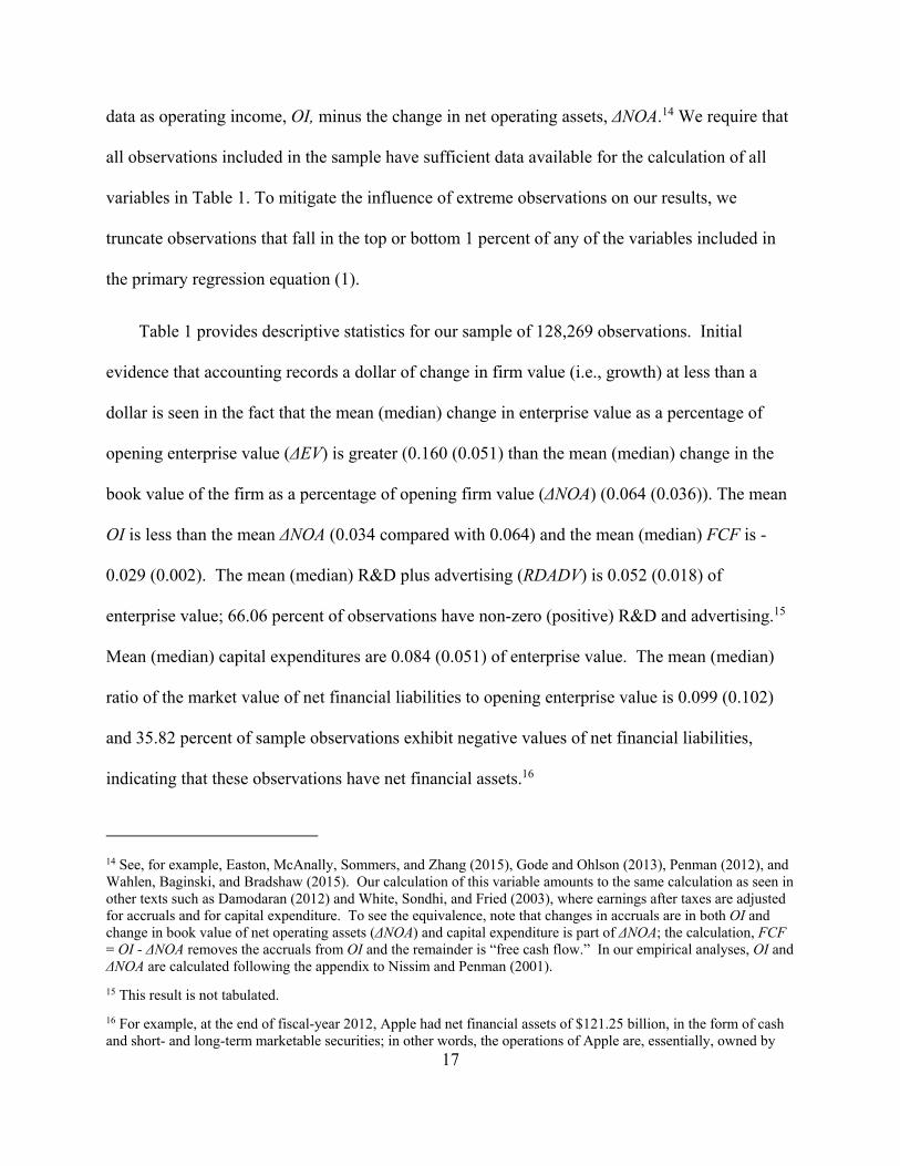
data as operating income, OI, minus the change in net operating assets, ΔNOA.14 We require that

all observations included in the sample have sufficient data available for the calculation of all

variables in Table 1. To mitigate the influence of extreme observations on our results, we

truncate observations that fall in the top or bottom 1 percent of any of the variables included in

the primary regression equation (1).

Table 1 provides descriptive statistics for our sample of 128,269 observations. Initial

evidence that accounting records a dollar of change in firm value (i.e., growth) at less than a

dollar is seen in the fact that the mean (median) change in enterprise value as a percentage of

opening enterprise value (ΔEV) is greater (0.160 (0.051) than the mean (median) change in the

book value of the firm as a percentage of opening firm value (ΔNOA) (0.064 (0.036)). The mean

OI is less than the mean ΔNOA (0.034 compared with 0.064) and the mean (median) FCF is -

0.029 (0.002). The mean (median) R&D plus advertising (RDADV) is 0.052 (0.018) of

enterprise value; 66.06 percent of observations have non-zero (positive) R&D and advertising.15

Mean (median) capital expenditures are 0.084 (0.051) of enterprise value. The mean (median)

ratio of the market value of net financial liabilities to opening enterprise value is 0.099 (0.102)

and 35.82 percent of sample observations exhibit negative values of net financial liabilities,

indicating that these observations have net financial assets.16

14 See, for example, Easton, McAnally, Sommers, and Zhang (2015), Gode and Ohlson (2013), Penman (2012), and Wahlen, Baginski, and Bradshaw (2015). Our calculation of this variable amounts to the same calculation as seen in other texts such as Damodaran (2012) and White, Sondhi, and Fried (2003), where earnings after taxes are adjusted for accruals and for capital expenditure. To see the equivalence, note that changes in accruals are in both OI and change in book value of net operating assets (ΔNOA) and capital expenditure is part of ΔNOA; the calculation, FCF = OI - ΔNOA removes the accruals from OI and the remainder is “free cash flow.” In our empirical analyses, OI and ΔNOA are calculated following the appendix to Nissim and Penman (2001).

15 This result is not tabulated.

16 For example, at the end of fiscal-year 2012, Apple had net financial assets of $121.25 billion, in the form of cash and short- and long-term marketable securities; in other words, the operations of Apple are, essentially, owned by

18

Table 2 reports correlations among key variables. We discuss some highlights from the

Spearman correlations. As expected the correlations between OI and RETent and OI and FCF are

both positive (0.418 and 0.284) and highly significant. The correlation between RETent and FCF

is significantly positive (0.157); that is, in general, higher firm returns are associated with more

cash outflow. We will refer back to this table when correlations among other variables become

pertinent to subsequent analyses and discussions.

V. Results: the Importance of Both the Source and Sign of Change in Firm Value

A basic premise of our paper is that the accounting for change in the market value of the

firm (i.e., growth) depends upon both the sign of the growth (i.e., growth vs. contraction) and the

source of the growth. To shed light on this premise we partition the sample into the six sub-

samples described in section III. Descriptive statistics and regression results for each of the six

sub-samples are summarized in Table 3. Panel A presents descriptive statistics for the sub-

samples. Panel B presents simple Spearman correlations. Panel C presents regression results

from estimating regression (1).

equity investors, who also own the net financial assets. We have heard arguments that this excess cash may be considered by some as part of the enterprise of Apple. We do not take this perspective because, again, we wish to focus on the entity where the change in value is not reported in the accounting at dollar-for-dollar. Elaborating further on this example, in 2012 Apple increased its cash dividend 10-fold acknowledging that it was returning some of the excess cash to the equity shareholders and in 2014, it returned $17 billion of its cash to equity holders in the form of share buy-backs. Neither of these transactions affected free cash flows; they were flows of funds from cash (which may be viewed as negative debt) to the equity shareholders who owned both the enterprise (i.e., the entity that produces smart phones, etc.) and the “pile of cash.”

19

Our primary contribution to the empirical understanding of recording of value change in

accounting earnings is through the introduction of cash flow to/from the capital providers to the

enterprise. There are several key results.

The relative magnitude of the effects of RETent and FCF on OI

The magnitude of the effect of FCF on recorded OI is, in many cases, equal to or greater

than the magnitude of the effect of returns on OI. We summarize these effects in Figure 1. We

plot the marginal effects of one-standard-deviation changes in RETent and FCF for each

regression sample, relative to one standard deviation of OI in each sample.17 In all but sub-

sample (6), where the firm is contracting on all dimensions and the coefficient relating OI to

FCF is not significantly different from zero, a one standard deviation change in FCF contributes

substantially to OI. In fact, for the full sample, the estimated effect of a one-standard deviation

change in FCF is slightly larger than the estimated effect of a one standard-deviation change in

RETent, such that a one standard deviation change in FCF is associated with a change of 30.30

percent of a standard deviation of OI while an equivalent change in RETent is associated with a

change of 17.90 percent. These estimated marginal effects are not statistically different from one

another, indicating that FCF explains a similar amount of EPAT variation as is explained by

RETent for the full sample.18 As further illustrated in Figure 1, the marginal effect of an FCF

17 Note that this is equivalent to normalizing the regression (1) variables to have a mean of zero and standard deviation of one within each regression sample and then plotting the absolute value of the normalized regression coefficients for RETent and FCF.

18 This is likely a conservative statement with respect to the relative importance of FCF in the full sample. The full-sample normalized coefficient on FCF is significantly different (two-tailed) from the normalized coefficient on RETent with high levels of statistical significance (p < 0.0000) when statistical significance is computed using a) unadjusted OLS standard errors, b) standard errors clustered by firm, or c) standard errors clustered by firm with fiscal year fixed effects included in the regression. Thus, FCF likely explains a greater portion of OI than RETent in the relevant population. Nevertheless, consistent with all other results presented in the paper, we report results based on standard errors clustered by both firm and year estimated using the “cluster2 ado” package in Stata.

20

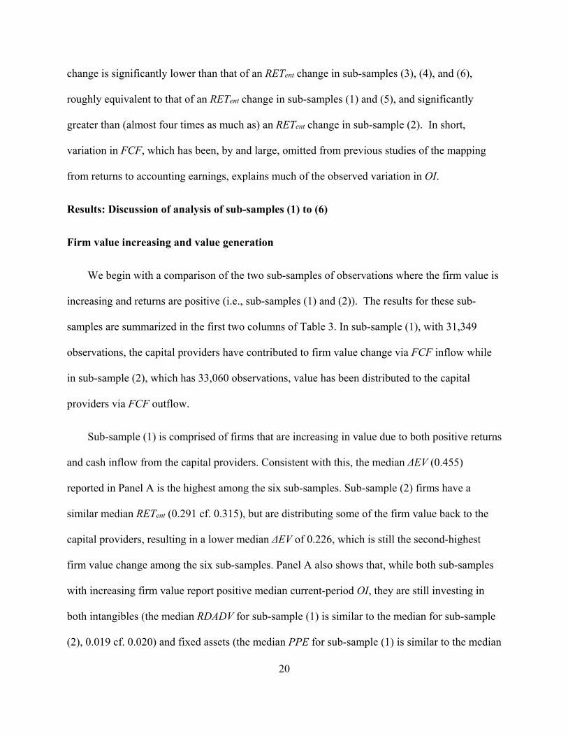
change is significantly lower than that of an RETent change in sub-samples (3), (4), and (6),

roughly equivalent to that of an RETent change in sub-samples (1) and (5), and significantly

greater than (almost four times as much as) an RETent change in sub-sample (2). In short,

variation in FCF, which has been, by and large, omitted from previous studies of the mapping

from returns to accounting earnings, explains much of the observed variation in OI.

Results: Discussion of analysis of sub-samples (1) to (6)

Firm value increasing and value generation

We begin with a comparison of the two sub-samples of observations where the firm value is

increasing and returns are positive (i.e., sub-samples (1) and (2)). The results for these sub-

samples are summarized in the first two columns of Table 3. In sub-sample (1), with 31,349

observations, the capital providers have contributed to firm value change via FCF inflow while

in sub-sample (2), which has 33,060 observations, value has been distributed to the capital

providers via FCF outflow.

Sub-sample (1) is comprised of firms that are increasing in value due to both positive returns

and cash inflow from the capital providers. Consistent with this, the median ΔEV (0.455)

reported in Panel A is the highest among the six sub-samples. Sub-sample (2) firms have a

similar median RETent (0.291 cf. 0.315), but are distributing some of the firm value back to the

capital providers, resulting in a lower median ΔEV of 0.226, which is still the second-highest

firm value change among the six sub-samples. Panel A also shows that, while both sub-samples

with increasing firm value report positive median current-period OI, they are still investing in

both intangibles (the median RDADV for sub-sample (1) is similar to the median for sub-sample

(2), 0.019 cf. 0.020) and fixed assets (the median PPE for sub-sample (1) is similar to the median

21

for sub-sample (2), 0.318 cf. 0.307). Most of the cash inflow in sub-sample (1) comes from debt

holders (median FCF of -0.098 and ΔNFL of 0.086) and much of the cash outflow in sub-sample

(2) goes to debt holders (median FCF of 0.059 and ΔNFL of -0.036). The firms that are

distributing cash to the capital providers are more than twice the size of those receiving cash

(median EV of $0.207 billion cf. $0.095 billion).

Turning to the simple correlations presented in Panel B, it is notable that the correlation

between OI and RETent is not significantly different from zero (-0.004) for sub-sample (1), but

positive and significant (0.256) for sub-sample (2). The correlation between OI and FCF for sub-

sample (1) is the lowest (0.058) among the six sub-samples, while the correlation between OI

and FCF for sub-sample (2) is the highest among the six sub-samples (0.315).

A summary of the results from the estimation of regression (1) is presented in Panel C. We

continue the comparison of the two sub-samples of observations where firm value is increasing

and returns are positive. The coefficient on RETent for sub-sample (1) is the smallest (i.e., least

positive) of the six sub-samples consistent with the notion that, in this sample where growth is

most evident, accounting captures net expenses (the estimate of the coefficient relating OI to

RETent is significantly negative, -0.038 with a t-statistic of -4.03), which are associated with the

generation of profits in future periods rather than in the current period. Further, we note that,

while the estimate of the coefficient on RETent is significantly negative for sub-sample (1), where

there is cash inflow, it is significantly positive for sub-sample (2) (0.016), when there is cash

outflow.19

19 The coefficient relating earnings to positive returns is generally not significantly different from zero in the analyses reported in the extant literature; our results of a significant negative coefficient when there is FCF inflow

22

The estimate of the coefficient on FCF (i.e., 0.123) in sub-sample (1) implies that

accounting records, in OI, 0.123 per dollar of FCF inflow. The estimate of the coefficient on

FCF in sub-sample (2), where FCF is positive, (i.e., there is net cash outflow) is much higher

than in sub-sample (1) (0.318 vs. 0.123); the higher coefficient in sub-sample (2) shows that

accounting records in OI more of cash outflows of firms that are increasing in value than of cash

inflows for firms that are increasing in value. Note that the inclusion of RETent in the regression

means that the estimate of the these coefficients on FCF capture the effect of the accounting in

reported OI. Absent conservative accounting, the coefficient would be zero; that is, conservative

accounting leads to 0.123 per dollar of FCF of expenses recorded in OI when there is FCF

inflow and 0.318 of additional reported income when there is FCF outflow. This 0.318 of

additional income arises because expenses are lower relative to sales (that is, income is higher)

due to conservative accounting, which has booked the related costs (R&D, advertising,

depreciation, etc.) in earlier periods (and, hence, expenses are conservatively low in the current

period).

In other words, the over-statement of the OI (i.e., net expense) effect of the FCF inflow is

less than the overstatement of the OI (i.e., net profit) effect when there is FCF outflow. The

characteristics of these sub-samples (see Panel A) provide indications of reasons for this

difference. A possible explanation is the fact that, although the firm value is increasing in both

sub-samples, the observations in sub-sample (1) have a median increase in NOA of 15.6 percent

of firm value while those in sub-sample (2) have virtually no change in NOA (0.015); that is,

much of the cash inflow is going to build assets but, not surprisingly (in light of the fact that the

(suggesting that expenses are greater than sales in the current period despite positive returns, which are indicating expectations of higher (and positive) changes in future profits) is an interesting addition to this literature.

23

firms in sub-sample (2) are also growing), cash outflow is not coming from sale of assets – rather

it is coming from OI of the period. This is consistent with the accumulation of the effects of

conservatism over time. That is, OI is overstated (and NOA understated) due to prior accelerated

depreciation of, or disallowed capitalization of, assets.

Firm contraction and value loss

Next we compare the two sub-samples (5 and 6) of observations where the firm value is

decreasing and returns are negative. In sub-sample (5), with 24,278 observations, the capital

providers have contributed to value change via FCF inflow; while in sub-sample (6), with 23,300

observations, FCF has been distributed to the capital providers. The results for sub-samples (5)

and (6) are summarized in the last two columns of Table 3.

The firms in sub-sample (5) are contracting due to loss in value of assets, but they continue

to receive support from the capital providers via FCF inflows. These are relatively small firms

(median EV of $0.094 billion compared with $0.145 for sub-sample (6)). These firms are, on

average, the most unprofitable across all six sub-samples (median OI of 0.003); they have higher

intangible intensity and much lower property plant and equipment than firms in sub-sample (6)

(median RDADV of 0.023 cf. 0.014 and mean PPE of 0.158 cf. 0.230). These firms have the

lowest mean BTM (0.385) of any of the six sub-samples; that is, the cumulative effects of

conservatism, as manifested in the balance sheet in relatively low book values, is greatest for

these firms. Consistent with the contraction experienced by these firms, they exhibit the highest

correlation between OI and RETent of the six sub-samples (0.416).

Moving to Panel C, the estimate of the coefficient on RETent in regression (1) of 0.174 for

sub-sample (5) indicates that there is a 17.4 cent loss in the current period per dollar of return,

while the estimate of this coefficient for sub-sample (6) is smaller (0.127); in other words, more

24

of the value lost relates to current earnings for the sub-sample of firms for which the capital

providers are contributing cash (presumably the capital providers see the loss in value as more

temporary and hence they are willing to contribute cash because of expected future return to

profitability) relative to those where the capital providers are removing cash. The striking feature

in the comparison across the results from sub-samples (5) and (6) is the difference in the

coefficients on FCF across these two samples of contracting firms. Much of cash inflow is

expensed in the current period (coefficient of 0.464), likely because it is going to research and

development, whereas there appears to be no evidence of conservatism in the accounting for cash

outflow (the estimate of the coefficient on FCF is not significantly different from zero).

Firm growth, value loss, net cash inflow

The results for sub-sample (3) are summarized in column (3) of Table 3. While firm growth

(contraction) is driven by returns for most firms, the firms in sub-sample (3) are experiencing

value increase due to large injections of cash by the capital providers despite experiencing

negative returns during the fiscal year. This is an unusual situation, evidenced by the fact that

sub-sample (3) is the smallest of the six sub-samples and only contains 5.81 percent of the

observations in the full sample (see Table 1, Panel B). The mean levels of EV in Panel A

indicate that sub-sample (3) contains, on average, the smallest firms in the sample, consistent

with these firms’ small market capitalization serving as a contributing factor in their ability to

grow the value of the firm by attracting additional capital despite experiencing value loss.

These firms are relatively unprofitable (median OI of 0.037), they invest little in intangibles

(lowest median RDADV of 0.013), and heavily in fixed assets (median PPE of 0.366). Because

of their high asset tangibility, these firms are able to raise a high percentage of their market value

25

from FCF inflows (most negative median FCF across all sub-samples, -0.212), resulting in large

increases in leverage (median ΔNFL of 0.191).

The results from estimation of regression (1) are summarized in Panel C. The estimate of

the coefficient on RETent (0.330) indicates that there is a 33.0 cent OI loss in the current period

per dollar of return. It is also interesting to note that the annual equity return is negative (i.e., in

Basu 1997 parlance, there is bad news) for most of the observations (7,043 of 7,449) in sub-

sample (3). Consistent with prior literature (e.g., Basu 1997), the estimate of the coefficients on

RETent is much higher (0.330, with a t-statistic of 8.91) for this sub-sample than for sub-samples

(1) and (2) where RETent was positive.20

The estimate of the coefficient on FCF (0.062) implies that there is little conservatism in the

accounting for FCF for these observations. This is consistent with the high levels of PPE in

these firms and indicates that the majority of the financing raised by these firms goes towards

investments that are capitalized into NOA (the implied coefficient relating ΔNOA to FCF, i.e. one

minus the estimated OI to FCF coefficient of 0.062, is 0.938).

Firm contraction, value generation, net cash outflow

The results for the analysis of sub-sample (4) are summarized in column (4) of Table 3.

Similar to sub-sample (3) this sub-sample is comprised of firms where the overall growth pattern

runs counter to return. In this case the firm is contracting despite positive returns, a somewhat

rare occurrence indicated by the fact that only 6.89 percent of our observations are in sub-sample

(4). Sub-sample (4) firms have high beginning-of-period leverage (median NFL of 0.362, which

20 These results are not tabulated.

26

is the highest among the six sub-samples). Despite experiencing positive median RETent of

0.058, these firms are contracting due to large cash outflows to the capital providers, generally

resulting in a deleveraging of the firm by returning capital to debt holders (median ΔNFL of -

0.094).

The results from estimation of regression (1) are reported in Panel C. The estimate of the

coefficient on RETent (0.256) indicates that there is a 25.6 cent profit in the current period per

dollar of generated value change. It is interesting to note that the coefficient on RETent is

significantly positive and relatively high (0.256, with t-statistics of 8.06); this, perhaps, seems

odd because RETent is positive (i.e., there is “good” news) and this, following the arguments in

Basu (1997) would suggest a lower RETent coefficient. In un-tabulated analysis, we penetrated

this result further by running the earnings/return regression as specified by Basu (1997); that is,

with an intercept and slope dummy, which is one if returns are negative, zero otherwise. The

estimate of the coefficient on positive returns is, contrary to the prediction in Basu (1997)

significantly positive (0.148 with a t-statistic of 2.89); that is, by considering the direction of net

transactions with the capital providers (positive vs. negative FCF), we have isolated a sample of

observations where equity returns are positive and there is a substantial estimated coefficient

relating earnings to return. In other words, for this sub-sample, the fact that cash is being paid

back to capital providers suggests that the positive return is due to more transitory changes in

profitability (and hence the high earnings/return coefficient).21 The key characteristic of this

sample is that the firms are contracting due to cash outflow despite returns, highlighting the

21 Note that the estimate of the RETent coefficient is lower in the other sub-samples in which RETent is positive (i.e., sub-samples (1) and (2)).

27

importance of considering overall firm growth as well as the direction of FCF in the analysis of

the mapping from change in value to accounting numbers.

The estimate of the coefficient on FCF (i.e., 0.046) implies that for each dollar of cash

outflow there is little conservatism in the accounting for OI for these observations. Perhaps the

most relevant comparison for this coefficient is that of sub-sample (2). Both sub-samples are

comprised of firms with positive returns, which are distributing cash to capital providers; firms

in sub-sample (4), however, are somewhat less profitable and make larger payouts that shrink the

size of the firm. Accordingly, firms in sub-sample (2) are able to source a larger percentage of

cash outflows from current OI relative to sub-sample (4) firms.

A summary of the results, which highlight the importance of consideration of the sign of FCF

First, as highlighted in the comparison of sub-samples (5) and (6) where the firm is

contracting, there is loss in value of the existing assets, and there is either cash outflow or cash

inflow, the extent to which cash flow affects the recording of OI varies a great deal (0.464 when

there is cash inflow and not significantly different from zero when there is cash outflow).

Second, the direction of cash flow affects the sign and magnitude of the coefficient relating

OI to RETent; in other words, identifying the direction of contributed/distributed value (FCF)

helps our understanding of the accounting for returns. This effect is best seen in the comparison

of the estimates of the coefficients relating OI to RETent across sub-samples (1) and (2), where

there is firm growth and generation of value from existing assets, and across sub-samples (5) and

(6), where there the firm is contracting and the is loss of value of the existing assets. Partitioning

growing firms (sub-samples (1) and (2)) on the sign of cash flow facilitates identification of a

significantly negative relation between OI and RETent when there is cash inflow (coefficient

28

estimate of -0.038 with a t-statistic of -4.03) and a significantly positive relation when there is

cash outflow (coefficient estimate of 0.016 with a t-statistic of 2.58). Partitioning contracting

firms (sub-samples (5) and (6)) on the sign of cash flow facilitates identification of a

significantly higher coefficient relating OI to RETent when there is cash inflow (0.174) than when

there is cash outflow (0.127); the (un-tabulated) t-statistic for the differences between these two

coefficient estimates is 2.71.

Third, our results highlight the role of overall firm growth/contraction in accounting for

value change when compared with the extant literature, which generally focuses on the relation

between accounting and equity returns. This point is best illustrated by sub-sample (4), which

isolates a sample of observations where equity returns are generally positive, but the estimated

coefficient relating OI to RETent is significantly positive and relatively high (0.256, with t-

statistics of 8.06). The key characteristic of this sample is that there is overall contraction due to

cash outflow despite positive RETent.

VI. Accounting for Change in Firm Value and Firm Characteristics: Leverage and the type of assets in which the firm invests

Motivation and research design

In this section, we show how the relation between OI and RETent and FCF varies with key

firm characteristics. Much work has been done on the effect of debt on the coefficient relating

earnings to returns. This work focuses on this coefficient when returns are negative (i.e., news is

bad); see, for example, Ball, Robin, and Sadka (2008), Khan and Watts (2009), and

Roychowdhury and Watts (2007). A larger coefficient relating earnings to negative returns is

generally observed when the debt level is higher.

29

Following this prior research, we also examine the role of debt (leverage) on the coefficients

relating OI to RETent and FCF. We will show that, when the firm is primarily owned by equity

holders (i.e., the debt/equity ratio is low), investment is primarily in intangibles (i.e., R&D and

advertising) and, when the firm is primarily owned by debt holders, investment is primarily in

property plant and equipment. This observation affects our predictions regarding the coefficients

relating OI to RETent and FCF across partitions of the data based on the ratio of debt to equity

ownership, and demonstrates that analyses based on the effects of debt capture differences in a

number of relevant characteristics; in particular differences in the types of investment and

difference in the accounting for different types of investments.

We perform two sets of analyses. First, by fiscal year, we partition the full sample into

leverage (NFL/EV) deciles. Within each decile, we report decile means and medians of relevant

firm characteristics. We also estimate regression (1) within each leverage decile. The results of

these analyses are presented in Table 4, and serve to demonstrate the general effects of leverage

on enterprise characteristics and on the relation between OI and changes in firm value.

We also examine the effects of leverage within each of the sub-samples (1) to (6) described

in section 3, since, as we have shown, the relation between OI and changes in firm value is also

affected by the sign and source of firm value change. These additional analyses are based on

regressions where we add interaction terms to regression (1). We interact each term in

regression (1) with DEC_NFL, the leverage decile ranking of the observation (as in Table 4),

30

scaled to have a mean of zero and a range of one.22 The formal regression specification is as

follows:

it= 1+ 2 3 it 4 _ it 5 ∗ _ it 6 it ∗

_ it εit (2)

The interpretation of the estimates of the coefficients 5 and 6 on the decile interaction terms is

that a coefficient estimate of, say, 0.1 on ∗ _ it implies the mapping from RETent

to OI increases/decreases by 0.01 for each decile of leverage above/below the mean sample

leverage. The results of these regressions are summarized in Table 5 for each of the sub-samples

(1) to (6) described in section III.

Results

Table 4, Panel A presents means and medians of key variables for each leverage decile. The

mean (median) portion of firm capital funded by debtholders (NFL/EV) increases from -0.64 (-

0.45) in decile 1, indicative of net financial assets, to 0.65 (0.65) in decile 10. The descriptive

statistics clearly indicate that investment in intangibles is highest when the firm is primarily

owned by equity holders. Mean (median) RDADV decreases monotonically from 0.13 (0.06) to

0.03 (0.00) as leverage increases from the lowest to highest decile. The descriptive statistics also

indicate that, when the firm is primarily owned by debt holders, investment is primarily in

property plant and equipment. The mean (median) PPE increases almost monotonically from

22 Specifically all observations in the lowest decile are coded -0.5, those in the next decile, -0.389, then -0.278, -0.167, -0.056, 0.056,….., 0.5. This decile rank transformation mitigates the effect of extreme observations and facilitates interpretation of the regression coefficients.

31

0.25 (0.13) in decile 2 to 0.56 (0.48) in decile 10. Finally, firm book-to-market (BTM) shows a

similar increase from 0.43 (0.29) in decile 2 to 1.02 (1.00) in decile 10.

Table 4, Panel B, presents the results of estimating regression (1) for each decile of

NFL/EV. The leverage effect documented in prior literature is clearly evident at the firm level,

demonstrated by the coefficients relating OI to RETent increasing monotonically from an

insignificant 0.14 in decile 1 to a highly significant 0.136 (t-statistic 8.19) in decile 10.

However, this result is unlikely to be driven solely by an increased demand for timeliness of

negative information by debtholders, which is the reason hypothesized in the extant literature.

The percentage of negative returns is fairly stable across deciles, and it decreases slightly

between lower and higher deciles of debt. In un-tabulated analyses, we also confirmed that the

documented increase in the RETent coefficient remains statistically and economically significant

when the sample is confined to only observations with positive returns. Furthermore, the results

in Panel B also demonstrate that the coefficient relating OI to FCF declines monotonically from

0.438 (t-statistic 13.56) in decile 1 to an insignificant 0.001 in decile 10. This is consistent with

firms with low leverage and high intangibles intensity in decile 1 expensing a high proportion of

FCF investments into OI, while the highly leveraged firms with more tangible FCF investments

in decile 10 do not expense investments of FCF into OI, rather they capitalize a higher

proportion of FCF investments in NOA.23

It is possible that these same differences in intangibles intensity and asset tangibility also

contribute to the increasing coefficient on RETent across leverage deciles discussed above.

23 The insignificant coefficient on FCF in decile 10 is also consistent with the BTM ratio for decile 10, which is close to 1 (Panel A), indicating that the book values of the enterprise assets for the firms in decile 10 are close to their market values.

32

Investments in intangibles are generally long-term investments with uncertain benefits and time

horizons, such that almost none of the value generated from these investments is recognized in

current income. On the other hand, investments in tangible assets may be associated with shorter

investment horizons, and some portion of the generated value from such projects may accrue to

current period earnings.

Table 5, Panel A, presents the results of estimating regression (2) including interaction terms

with DEC_NFL for each of our six growth partitions. Prior work focuses particularly on the

effect of leverage on the relation between earnings and returns when returns are negative (i.e.,

news is bad); see, for example, Ball, Robin, and Sadka (2008) and Khan and Watts (2009). This

work generally observes a larger coefficient relating earnings to negative returns when the debt

level is higher. We observe a similar pattern for the coefficient relating OI to RETent. This is

evidenced by the positive coefficient on RETent *DEC_NFL in sub-sample (6), where RETent is

negative (coefficient estimate of 0.143, with a t-statistic of 7.48). Interestingly, a new insight

emerges from a comparison of sub-sample (5), where RETent is negative and there is cash inflow,

with sub-sample (6), where RETent is negative but there is cash outflow; in contrast to the

estimate of the coefficient on RETent *DEC_NFL when there is cash outflow, the estimate of this

coefficient when there is cash inflow is not significantly different from zero (0.019 with a t-

statistic of 0.56). Since the amount of debt is much smaller for this sub-sample, (median

NFL/EV of 0.003 compared with 0.139), this result may serve as evidence of the effect of debt

postulated in the literature (i.e., the greater the debt, the greater the demand for accounting

conservatism); on the other hand, this coefficient may reflect the fact that there is almost twice as

much R&D in subsample (5) compared with sub-sample (6) – (0.023 cf. 0.014) and much less

property, plant and equipment (0.158 cf. 0.230).

33

The estimated coefficients on RETent *DEC_NFL are also significantly positive (0.079 and

0.039) for sub-samples (1) and (2) where RETent is positive. This result is new to the literature as

far as we are aware; the extent to which returns are captured in current OI increases with debt

level when the firm is doing well and when the firm is doing poorly.

The estimates of the coefficient on FCF*DEC_NFL are negative and significant for all six

sub-samples. This suggests that, when firms have higher levels of debt, FCF inflows are more

likely to be capitalized into NOA than expensed to OI, and that FCF outflows are more likely to

come from liquidating NOA than from current OI, consistent with the results discussed above in

Table 4.

VII. Summary and conclusions

We focus on the recording of change in firm value in the financial statements. This

motivates two fundamental changes to the methodology at the core of the vast empirical

literature examining the extent to which accounting captures concurrent changes in market value.

First, we bring the focus to the part of the earnings/returns relation that is not dollar-for-dollar

because, at best, the part that is recorded dollar-for-dollar is uninteresting empirically and, at

worst, including this part may lead to incorrect inferences. Second, we suggest the inclusion of

cash flows in the earnings/change in value relation. This additional variable captures an aspect of

accounting that has not been examined in prior studies, the accounting for growth/contraction

due to transactions with capital providers.

We show that this additional source of value change explains a considerable portion of

operating income; in fact, for the sub-sample of observations where there is growth due to

34

change in the value of assets in place yet there is net cash outflow to the capital providers, free

cash flow explains almost four times that which is explained by returns Adding this dimension of

change in value may considerably enhance studies which have to-date relied on the earnings-

return relation. Vassallo and Taylor (2015), for example, show that the estimates of the

coefficients relating operating income to both returns and free cash flows vary, as expected, with

audit quality.

Much of our analysis focuses on partitions of the data based on the sign and source of

change in value. We argue and show that accounting for value change (growth) depends, not

only on the direction (expansion vs. contraction) of the value change, but also on the source of

the value change.

We illustrate the importance of: (1) focusing on operating income and change in firm value;

and, (2) adding free cash flow to the earnings/return regression, by partitioning on the

debt/equity ratio and showing how the firm assets differ across these partitions and, in turn, the

accounting (i.e., the portion of returns and free cash flow that is captured in operating income)

differs. An implication of this finding is that conclusions in the extant literature regarding the

influence of, for example, contracting, may be premature; the difference may reflect no more

than differences in the accounting for different assets (e.g., full expensing of investment in R&D,

which tends to be the primary form of investment when the firm is mostly owned by equity

holders) vs. capitalizing investment in property, plant and equipment, which tends to be the

primary form of investment when the firm is owned by debt holders).

35

References

Ball, R., and P. Brown. 1967. Some preliminary findings on the association between earnings of a firm, its industry, and the economy. Journal of Accounting Research 5: 50-77.

Ball, R., and P. Brown. 1968. An empirical evaluation of accounting income numbers. Journal of Accounting Research 6: 159-178.

Ball, R., S. Kothari, and V. Nikolaev. 2013. On estimating conditional conservatism. The Accounting Review 88 (3): 755-787.

Ball, R., A. Robin, and G. Sadka. 2008. Is financial reporting shaped by equity markets or by debt markets? An international study of timeliness and conservatism. Review of Accounting Studies 13: 168-205.

Basu, S. 1997. The conservatism principle and the asymmetric timeliness of earnings. Journal of Accounting and Economics 24: 3-37.

Beaver, W., R. Lambert, and S. Ryan. 1987. The Information Content of Security Prices: A Second Look. Journal of Accounting and Economics 9 (2) 109-228.

Collins, D., P Hribar, and X. Tian. 2014. Cash flow asymmetry: Causes and implications for conditional conservatism research. Journal of Accounting and Economics 58: 173 – 200.

Damodaran, A. 2012. Investment Valuation: Tools and Techniques for Determining the Value of Any Asset. 3rd Edition. Hoboken, NJ: John Wiley & Sons, Inc.

Easton, P. 2009. Discussion of: Accounting data and value: The basic results. Contemporary Accounting Research 26: 261-272.

Easton, P. 2016. Financial Reporting: An enterprise operations perspective. Journal of Financial Reporting (in press).

Easton, P., and T. Harris. 1991. Earnings as an explanatory variable for returns. Journal of Accounting Research 29: 19-36.

Easton, P., M. McAnally, G. Sommers, and X. Zhang. 2015. Financial Statement Analysis and Valuation. 5th Edition. Westmont IL: Cambridge Business Publishers.

Easton, P., and J. Pae. 2004. Accounting conservatism and the relation between returns and accounting data. Review of Accounting Studies 9: 495-522.

Feltham, G., and J. Ohlson. 1995. Valuation and clean surplus accounting for operating and financial activities. Contemporary Accounting Research 11: 689-731.

Feltham, G., and J. Ohlson. 1996. Uncertainty resolution and the theory of depreciation measurement. Journal of Accounting Research 34: 209-234.

Feltham, G., and J. Ohlson. 1999. Residual earnings valuation with risk and stochastic interest rates. The Accounting Review 74: 165-183.

36

Gode, D., and J. Ohlson. 2013. Financial Statement Analysis and Valuation. Available at http://www.godeohlson.com/. (Last access December 28, 2014).

Khan, M., and R. Watts. 2009. Estimation and empirical properties of a firm-year measure of accounting conservatism. Journal of Accounting and Economics 48: 132-150.

Lawrence, A., R. Sloan, and Y. Sun. 2015. Why are Losses Less Persistent than Profits? Curtailments versus Conservatism. Working paper, University of California, Berkeley.

Modigliani, F. and M. Miller. 1958. The Cost of Capital, Corporation Finance and the Theory of Investment. The American Economic Review 48 (3) 261-297.

Nissim, D., and S. Penman. 2001. Ratio analysis and equity valuation: From research to practice. Review of Accounting Studies 6: 109-154.

Ohlson, J. 2009. Accounting data and value: The basic results. Contemporary Accounting Research 26: 231-259.

Penman, S. 2012. Financial Statement Analysis and Security Valuation. 5th Edition. New York City, New York: McGraw-Hill Education.

Penman, S., and N. Yehuda. 2009. The pricing of earnings and cash flows and an affirmation of accrual accounting. Review of Accounting Studies 14: 453-479.

Roychowdhury, S., and R. Watts. 2007. Asymmetric timeliness of earnings, market-to-book and conservatism in financial reporting. Journal of Accounting and Economics 44: 2–31.

Vassallo, P., and S. Taylor. 2015. A Cash Flow Perspective on Accounting Conservatism. Working paper, University of New South Wales.

Wahlen, J., S. Baginski, and M. Bradshaw. 2015. Financial Reporting, Financial Statement Analysis, and Valuation. 8th Edition. Boston, MA: Cengage Learning.

White, G., A. Sondhi, and D. Fried. 2003. The Analysis and Use of Financial Statements. 3rd Edition. Hoboken, NJ: John Wiley & Sons, Inc.

Zhang, X. 2000. Conservative accounting and equity valuation. Journal of Accounting and Economics 29: 125-149.

37

Appendix: Variable Definitions

# = Compustat Data Item.

Δ = Change between current and prior fiscal year.

BTM = Enterprise Book-to-Market = Beginning-of-period Net Operating Assets (NOAt-1) divided by beginning-of-period Enterprise Value (EVt-1).

CNFI = Comprehensive Net Financial Income = Comprehensive Net Income (CNI) minus Enterprise Profit After Tax (OI).

CNI = Comprehensive Net Income = Net Income (#NI) minus preferred dividends (#DVP) plus Clean Surplus Adjustment to Net Income (CSA).

CSA = Clean Surplus Adjustment to Net Income = marketable securities adjustment (#MSA) minus lag marketable securities adjustment (#MSAt-1) plus cumulative translation adjustment (#RECTA) minus lag cumulative translation adjustment (#RECTAt-1).

CSE = Common Stockholders’ Equity = Common equity (#CEQ) plus preferred treasury stock (#TSTKP) minus preferred dividends in arrears (#DVPA).

EV = Enterprise Value = Market Value of Equity (MVE) plus Net Financial Liabilities (NFL).

FA = Financial Assets = Cash and short term investments (#CHE) plus investments and advances-other (#IVAO).

FCF = Free Cash Flow = Operating Income (OI) minus change in Net Operating Assets Assets (ΔNOA). Scaled by beginning-of-period enterprise value (EVt-1).

FL = Financial Liabilities = Debt in current liabilities (#DLC) plus long term debt (#DLTT) plus preferred stock (#PSTK) minus preferred treasury stock (#TSTKP) plus preferred dividends in arrears (#DVPA).

Marginal Tax Rate = The top statutory federal corporate tax rate plus 2% average state corporate tax rate. The top statutory federal corporate tax rate was 52% in 1963, 50% in 1964, 48% in 1965 – 1967, 52.8% in 1968 – 1969, 49.2% in 1970, 48% in 1971 – 1978, 46% in 1979 – 1986, 40% in 1987, 34% in 1988 – 1992 and 35% in all sample years thereafter.

MVE = Market Value of Equity = Fiscal year end price (#PRCC_F) times common shares outstanding (#CSHO), from Compustat. Scaled by beginning-of-period enterprise value (EVt-1).

NFE = Net Financial Expense = After-tax interest expense ((#XINT)*(1 – marginal tax rate)) plus preferred dividends (#DVP) minus after tax interest income ((#IDIT)*(1-marginal tax rate)) plus unusual financial expense ((#MSAt-1)-(#MSA)).

NFL = Net Financial Liabilities = Financial Liabilities (FL) minus Financial Assets (FA). Scaled by beginning-of-period enterprise value (EVt-1).

38

NOA = Net Operating Assets = Net Financial Liabilities (NFL) plus Common Stockholders’ Equity (CSE) plus Minority Interest (#MIB). Scaled by beginning-of-period enterprise value (EVt-1).

OI = Operating Income = Comprehensive Net Income (CNI) plus Net Financial Expense (NFE) plus minority interest in income (#MII). Scaled by beginning-of-period enterprise value (EVt-1).

PPE = Property Plant and Equipment = Property plant and equipment, net of accumulated depreciation (#PPENT). Scaled by beginning-of-period enterprise value (EVt-1).

RDADV = Research, Development, and Advertising = R&D Expense (#XRD) plus Advertising Expense (#XAD). Scaled by beginning-of-period enterprise value (EVt-1).

RETent = Enterprise (firm) Return = Change in Enterprise Value (ΔEV) plus Free Cash Flow (FCF). Scaled by beginning-of-period enterprise value (EVt-1).

39

Table 1

Descriptive Statistics

Panel A: Full sample descriptive statistics N Mean σ p1 p25 Median p75 p99 EV ($ Bil.) 128,269 1.761 11.705 0.003 0.032 0.120 0.574 29.387 ΔEV 128,269 0.160 0.628 -0.761 -0.175 0.051 0.341 2.401 ΔNOA 128,269 0.064 0.207 -0.434 -0.020 0.036 0.124 0.830 OI 128,269 0.034 0.136 -0.479 0.007 0.057 0.096 0.297 RETent 128,269 0.131 0.596 -0.853 -0.171 0.056 0.309 2.225 FCF 128,269 -0.029 0.203 -0.802 -0.090 0.002 0.068 0.402 RDADV 128,269 0.052 0.110 0.000 0.000 0.018 0.063 0.449 CAPX 128,269 0.084 0.111 0.000 0.022 0.051 0.104 0.525 PPE 128,269 0.386 0.389 0.005 0.107 0.272 0.544 1.694 NFL 128,269 0.099 0.426 -1.194 -0.071 0.102 0.332 0.821 ΔNFL 128,269 0.027 0.194 -0.431 -0.054 0.008 0.085 0.722 BTM 128,269 0.679 0.516 -0.039 0.309 0.613 0.957 2.227 |NFE|/MVE 128,269 0.034 0.079 0.000 0.003 0.012 0.035 0.312

Panel B: Frequencies among firm growth sub-samples

(1) (2) (3) (4) (5) (6) + ΔEV

+ RETent FCF in

+ ΔEV + RETent FCF out

+ ΔEV - RETent FCF in

- ΔEV + RETent FCF out

- ΔEV - RETent FCF in

- ΔEV - RETent FCF out Total

N 31,349 33,060 7,449 8,833 24,278 23,300 128,269 Pct (%) 24.44 25.77 5.81 6.89 18.93 18.16 100

This table presents descriptive statistics for the full sample of observations used in our analysis. Panel A presents sample statistics. σ and p denote the sample standard deviation and percentiles, respectively. Panel B presents frequencies of observations within each enterprise growth sub-sample used in our empirical analyses. As described in Section III of the text, we partition the full sample into six enterprise growth sub-samples based on the sign of ΔEV, RETent, and FCF. A positive (negative) sign denotes that observations in the sub-sample are restricted to those where the corresponding variable is greater than or equal to zero (less than zero). All variables are defined in Appendix A. .

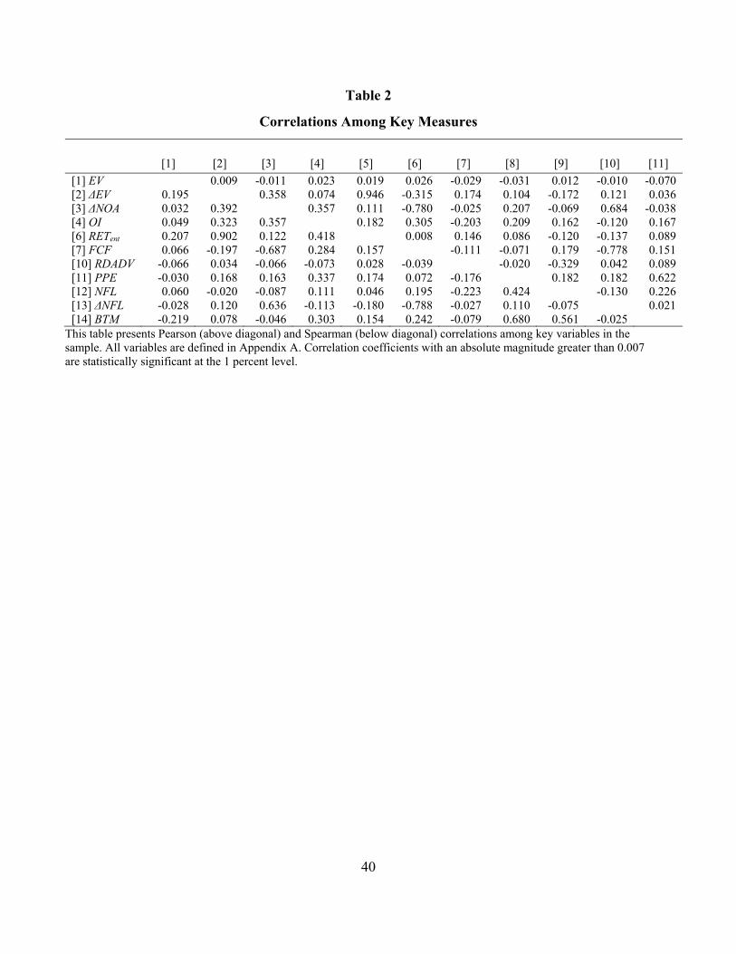
40

Table 2

Correlations Among Key Measures

[1] [2] [3] [4] [5] [6] [7] [8] [9] [10] [11]

[1] EV 0.009 -0.011 0.023 0.019 0.026 -0.029 -0.031 0.012 -0.010 -0.070 [2] ΔEV 0.195 0.358 0.074 0.946 -0.315 0.174 0.104 -0.172 0.121 0.036 [3] ΔNOA 0.032 0.392 0.357 0.111 -0.780 -0.025 0.207 -0.069 0.684 -0.038 [4] OI 0.049 0.323 0.357 0.182 0.305 -0.203 0.209 0.162 -0.120 0.167 [6] RETent 0.207 0.902 0.122 0.418 0.008 0.146 0.086 -0.120 -0.137 0.089 [7] FCF 0.066 -0.197 -0.687 0.284 0.157 -0.111 -0.071 0.179 -0.778 0.151 [10] RDADV -0.066 0.034 -0.066 -0.073 0.028 -0.039 -0.020 -0.329 0.042 0.089 [11] PPE -0.030 0.168 0.163 0.337 0.174 0.072 -0.176 0.182 0.182 0.622 [12] NFL 0.060 -0.020 -0.087 0.111 0.046 0.195 -0.223 0.424 -0.130 0.226 [13] ΔNFL -0.028 0.120 0.636 -0.113 -0.180 -0.788 -0.027 0.110 -0.075 0.021 [14] BTM -0.219 0.078 -0.046 0.303 0.154 0.242 -0.079 0.680 0.561 -0.025

This table presents Pearson (above diagonal) and Spearman (below diagonal) correlations among key variables in the sample. All variables are defined in Appendix A. Correlation coefficients with an absolute magnitude greater than 0.007 are statistically significant at the 1 percent level.

41

Table 3

Summary of Results by Sub-Sample

(1) (2) (3) (4) (5) (6) + ΔEV

+ RETent FCF in

+ ΔEV + RETent FCF out

+ ΔEV - RETent FCF in

- ΔEV + RETent FCF out

- ΔEV - RETent FCF in

- ΔEV - RETent FCF out

Panel A: Sample Medians for Key Measures EV ($ Bil.) 0.095 0.207 0.069 0.109 0.094 0.145 ΔEV 0.455 0.226 0.098 -0.062 -0.250 -0.244 ΔNOA 0.156 0.015 0.215 -0.066 0.059 -0.011 OI 0.066 0.083 0.037 0.075 0.003 0.045 RETent 0.291 0.315 -0.082 0.058 -0.355 -0.158 FCF -0.098 0.064 -0.212 0.141 -0.066 0.052 RDADV 0.019 0.020 0.013 0.013 0.023 0.014 PPE 0.318 0.307 0.366 0.401 0.158 0.230 NFL 0.092 0.121 0.130 0.362 0.003 0.139 ΔNFL 0.086 -0.039 0.191 -0.094 0.062 -0.028 BTM 0.602 0.686 0.656 0.979 0.385 0.633 |NFE|/MVE 0.013 0.011 0.020 0.031 0.007 0.011 Panel B: Spearman Correlations between Key Measures OI & RETent -0.004 0.256 0.209 0.270 0.416 0.238 OI & FCF 0.058 0.315 0.130 0.207 0.258 0.119 RETent & FCF -0.151 0.343 0.632 0.609 0.395 0.181 RETent & RDADV 0.112 0.123 -0.057 0.045 -0.157 -0.062 RETent & PPE -0.151 -0.080 0.020 0.128 0.349 0.309 RETent & NFL -0.303 -0.288 0.275 0.032 0.432 0.342 RETent & ΔNFL -0.196 -0.373 -0.247 -0.474 -0.071 -0.024 RETent & BTM -0.212 -0.043 0.137 0.302 0.369 0.306 FCF & RDADV -0.021 0.075 -0.035 0.025 -0.139 -0.022 FCF & PPE -0.119 0.171 -0.071 0.152 0.017 0.174 FCF & NFL 0.068 0.021 0.200 0.157 0.229 0.206 FCF & ΔNFL -0.417 -0.619 -0.422 -0.755 -0.482 -0.703 FCF & BTM -0.055 0.311 0.051 0.428 0.067 0.385 PPE & RDADV -0.223 -0.123 -0.251 -0.079 -0.256 -0.155 PPE & NFL 0.423 0.411 0.362 0.287 0.445 0.394 PPE & ΔNFL 0.394 0.066 0.322 -0.056 0.286 0.016 PPE & BTM 0.678 0.696 0.599 0.558 0.700 0.638 NFL & ΔNFL 0.186 0.059 0.080 -0.149 0.013 -0.120 NFL & BTM 0.534 0.524 0.500 0.503 0.526 0.575 ΔNFL & BTM 0.419 -0.039 0.315 -0.311 0.283 -0.169 EV & BTM -0.234 -0.407 -0.141 -0.458 -0.070 -0.318 Observations 31,349 33,060 7,449 8,833 24,278 23,300

42

Table 3 (continued)

Summary of Results by Sub-Sample

(1) (2) (3) (4) (5) (6) + ΔEV

+ RETent FCF in

+ ΔEV + RETent FCF out

+ ΔEV - RETent FCF in

- ΔEV + RETent FCF out

- ΔEV - RETent FCF in

- ΔEV - RETent FCF out

Panel C: Estimates of Regression (1) Intercept 0.079*** 0.056*** 0.039*** 0.045*** 0.075*** 0.056*** (9.92) (14.82) (4.80) (11.37) (9.74) (16.87) RETent -0.038*** 0.016*** 0.330*** 0.256*** 0.174*** 0.127*** (-4.03) (2.58) (8.91) (8.06) (11.93) (8.80) FCF 0.123*** 0.318*** 0.062*** 0.046* 0.464*** -0.054 (4.65) (7.01) (3.44) (1.89) (10.93) (-1.50) Adjusted R2 0.076 0.121 0.101 0.081 0.268 0.043

This table provides descriptive statistics and OLS regression estimates for each firm growth sub-sample. Each column presents results for one of the firm growth sub-samples (1) – (6) defined in Table 1. Panel A presents the sub-sample medians for key variables. Panel B presents univariate correlations between key variables within each sub-sample. Correlations presented in bold typeface are statistically significant at the 1 percent level. Panel C reports the estimated coefficients and adjusted R2 from estimating regression (1) on each sub-sample. The dependent measure in these regressions is OI. All variables are defined in Appendix A. t-statistics reported in parenthesis are calculated using two-way clustered standard errors, clustered by firm and year. *, ** and *** indicate (two-tailed) significance at the 10 percent, 5 percent and 1 percent levels respectively.

43

Table 4 Effects of Leverage

NFL Deciles

Low Leverage

(2) (3) (4) (5) (6) (7) (8) (9) High Leverage

Panel A: Decile Means (Medians) for Key Measures

NFL -0.64 -0.17 -0.07 0.00 0.07 0.14 0.23 0.33 0.45 0.65 (-0.45) (-0.17) (-0.07) (-0.01) (0.05) (0.13) (0.21) (0.32) (0.44) (0.65) RDADV 0.13 0.07 0.05 0.04 0.04 0.04 0.04 0.03 0.03 0.03 (0.06) (0.04) (0.03) (0.02) (0.02) (0.02) (0.01) (0.01) (0.01) (0.00) CAPX 0.10 0.07 0.07 0.07 0.08 0.09 0.09 0.10 0.10 0.09 (0.05) (0.04) (0.04) (0.04) (0.05) (0.06) (0.06) (0.07) (0.06) (0.05) PPE 0.38 0.25 0.24 0.27 0.32 0.37 0.44 0.50 0.54 0.56 (0.21) (0.13) (0.14) (0.16) (0.22) (0.29) (0.35) (0.42) (0.45) (0.48) BTM 0.68 0.43 0.41 0.46 0.55 0.66 0.76 0.86 0.96 1.02 (0.45) (0.29) (0.29) (0.35) (0.46) (0.57) (0.68) (0.79) (0.91) (1.00)

Panel B: Estimates of Regression (1) Intercept 0.041*** 0.032*** 0.034*** 0.040*** 0.044*** 0.045*** 0.043*** 0.036*** 0.028*** 0.017*** (3.31) (4.70) (5.44) (6.81) (8.02) (8.50) (9.08) (7.49) (5.78) (3.82) RETent 0.014 0.031*** 0.040*** 0.045*** 0.050*** 0.068*** 0.077*** 0.096*** 0.110*** 0.136*** (0.86) (2.83) (3.77) (4.53) (3.86) (7.06) (7.93) (8.30) (7.76) (8.19) FCF 0.438*** 0.341*** 0.274*** 0.208*** 0.186*** 0.117*** 0.089*** 0.062*** 0.041*** 0.001 (13.56) (12.60) (13.32) (12.31) (10.82) (8.83) (9.47) (6.93) (5.06) (0.16) Adjusted R2 0.267 0.219 0.184 0.161 0.149 0.137 0.113 0.114 0.105 0.108 Observations 12,806 12,832 12,832 12,830 12,821 12,844 12,831 12,831 12,833 12,809

This table provides descriptive statistics and OLS regression estimates within each decile of NFL in the full sample. Observations are ranked into deciles each fiscal year. Panel A presents decile means (medians) for key variables. Panel B reports the estimated coefficients and adjusted R2 from estimating regression (1) within each decile. The dependent measure in these regressions is EPAT. All variables are defined in Appendix A. t-statistics reported in parenthesis in Panel B are calculated using two-way clustered standard errors, clustered by firm and year. *, ** and *** indicate (two-tailed) significance at the 10 percent, 5 percent and 1 percent levels respectively.

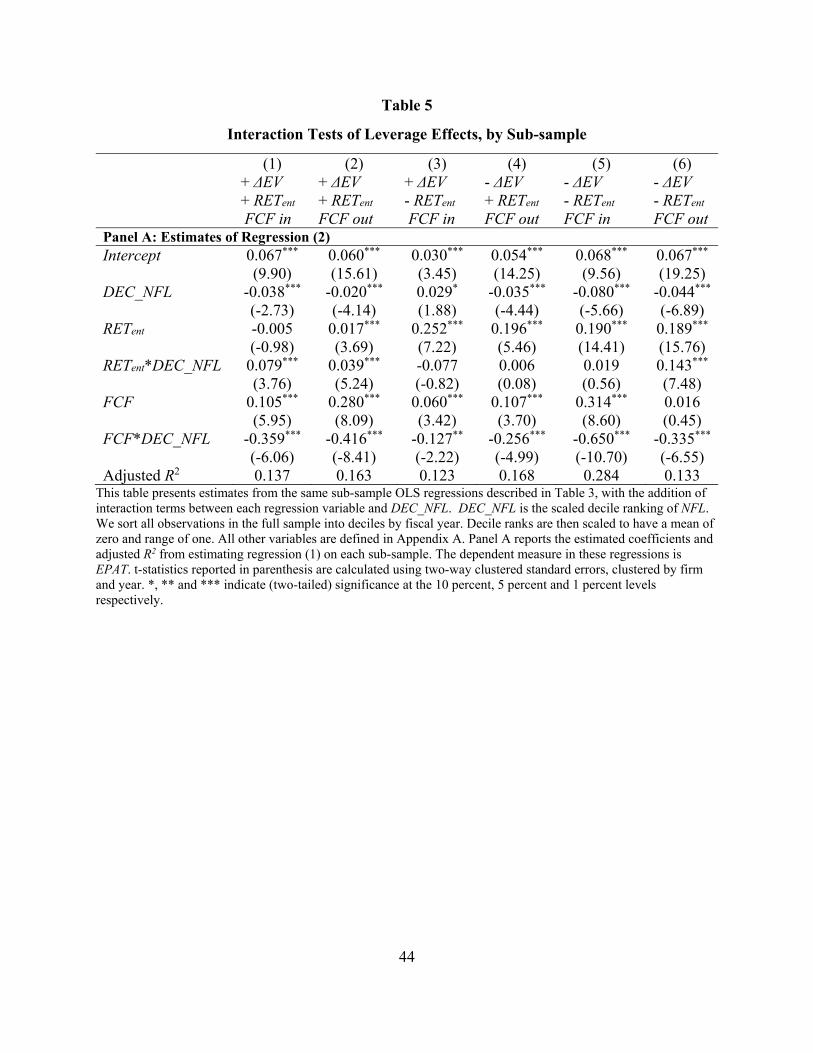
44

Table 5

Interaction Tests of Leverage Effects, by Sub-sample

(1) (2) (3) (4) (5) (6) + ΔEV

+ RETent FCF in

+ ΔEV + RETent FCF out

+ ΔEV - RETent FCF in

- ΔEV + RETent FCF out

- ΔEV - RETent FCF in

- ΔEV - RETent FCF out

Panel A: Estimates of Regression (2) Intercept 0.067*** 0.060*** 0.030*** 0.054*** 0.068*** 0.067*** (9.90) (15.61) (3.45) (14.25) (9.56) (19.25) DEC_NFL -0.038*** -0.020*** 0.029* -0.035*** -0.080*** -0.044*** (-2.73) (-4.14) (1.88) (-4.44) (-5.66) (-6.89) RETent -0.005 0.017*** 0.252*** 0.196*** 0.190*** 0.189*** (-0.98) (3.69) (7.22) (5.46) (14.41) (15.76) RETent*DEC_NFL 0.079*** 0.039*** -0.077 0.006 0.019 0.143*** (3.76) (5.24) (-0.82) (0.08) (0.56) (7.48) FCF 0.105*** 0.280*** 0.060*** 0.107*** 0.314*** 0.016 (5.95) (8.09) (3.42) (3.70) (8.60) (0.45) FCF*DEC_NFL -0.359*** -0.416*** -0.127** -0.256*** -0.650*** -0.335*** (-6.06) (-8.41) (-2.22) (-4.99) (-10.70) (-6.55) Adjusted R2 0.137 0.163 0.123 0.168 0.284 0.133

This table presents estimates from the same sub-sample OLS regressions described in Table 3, with the addition of interaction terms between each regression variable and DEC_NFL. DEC_NFL is the scaled decile ranking of NFL. We sort all observations in the full sample into deciles by fiscal year. Decile ranks are then scaled to have a mean of zero and range of one. All other variables are defined in Appendix A. Panel A reports the estimated coefficients and adjusted R2 from estimating regression (1) on each sub-sample. The dependent measure in these regressions is EPAT. t-statistics reported in parenthesis are calculated using two-way clustered standard errors, clustered by firm and year. *, ** and *** indicate (two-tailed) significance at the 10 percent, 5 percent and 1 percent levels respectively.

45

Figure 1

Normalized marginal effects of changes in enterprise value on estimated EPAT

This figure presents the marginal effects of a one standard deviation change in enterprise value on OI. Each column plots the magnitude of the effect of a one standard deviation change in RETent or FCF on OI based on the estimated coefficients from regression (2) for each regression sample listed along the horizontal axis. The regression sub-samples are defined in Table 1. The height of each column is scaled by the standard deviation of OI for the corresponding sample, facilitating comparison across sub-samples. This is equivalent to normalizing all regression variables within each regression sample and plotting the (absolute) normalized coefficients. *, ** and *** indicate that the heights of the two columns for the corresponding sample are significantly different at the (two-tailed) 10 percent, 5 percent and 1 percent levels respectively, based on Wald tests of the corresponding normalized regression coefficients.

0%

10%

20%

30%

40%

50%

60%

FullSample

+EV+RETentFCF in

+EV+RETentFCF out

***

+EV-RETentFCF in

***

-EV+RETentFCF out

***

-EV-RETentECF in

-EV-RETentFCF out

***

Est

imat

ed m

argi

nal

eff

ect

as a

%

of o

ne

OI

std

. dev

.

RETent FCF