Accessing Genomic Databases with RAccessing Genomic Databases with RIIHG Bioinformatics Spring 2020 WorkshopIIHG Bioinformatics Spring 2020 Workshop

Jason RatcliffJason Ratcliff

2020-04-152020-04-15

1 / 561 / 56

Tidyverse

Ecosystem of packages for datascience

dplyr, purrr, tibble, ggplot2Data structures and functions

Tibble data framesThe %>% pipe operator

R Markdown

Framework for reproducibleresearchReport generation

Bookdown

# CRAN installs for data wranglinginstall.packages("magrittr") # pipe %>%install.packages("tidyverse")

getwd()

## [1] "/Users/jratcliff/Bioinformatics/Workshops"

Create directory for GEOqueryMore on that later...

# Relative path for storing GEO downloadsdir.create("geoData")

A Brief Orientation to RR Resources

     Working Directory

2 / 56

Installing BioconductorInstallation prerequisites

R version 3.5RStudio IDE

# Install the main Bioconductor Managaement package from CRANinstall.packages("BiocManager")

For a minimal, core installation:Use the install() function with no arguments

If prompted to update packages, go aheadIncludes: Biobase, BioGenerics, BiocParallel

BiocManager::install()

Use install() for additional Bioconductor packagesInstall multiple packages using a character vector of package names

BiocManager::install(c("GEOquery", "rentrez", "IRanges", "GenomicRanges", "Biostrings", "rtracklayer", "Gviz", "AnnotationHub"))

3 / 56

What is Bioconductor?

Collection of:

data structuresanalysis methods

Variety of packages

SoftwareAnnotationsExperimentWorkflow

Emphasizes reproducible research

Credit for code | Nature Genetics

Open Development

Anyone can contribute or participatein code development

Formal review framework forpackage submissions

Open Source

Code is freely available to read ormodify

Bioconductor Overview | Website

R LanguageFlexible programming language geared towards data analysis

High quality graphics frameworkGood interoperability with tools from other languages

Python, SQLC / C++

4 / 56

NCBI Gene Expression Omnibus (GEO)Public repository for high-throughput gene expression and genomic data

MicroarraysNext-generation sequencing

Methyl-seq / ChIP-seq / ATAC-seqProteomics

Mass spectrometry

GEO Overview

Summary of Public HoldingsAvailable Platforms

Designing Queries

Outlines query construction for searching the GEO databaseCan be paired with rentrez for identifying GEO accessions

5 / 56

Datasets | GDS[0-9]+Curated set of GEO sample data (GDS)

Links a set of comparable GEO SamplesSamples in a given GDS share the same Platform

Measurement methodology is assumed to be consistenti.e. background corrections or normalization

6 / 56

Records information about asingle Sample

Cell line / tissueExperiment groupsData analysisLaboratory methods

References a single Platform

May be in multiple Series

Sample | GSM[0-9]+

7 / 56

Platform | GPL[0-9]+Provides a summary description of the experimental Platform

MicroarraySequencer

A Platform ID is not limited to a single sample or submitter

8 / 56

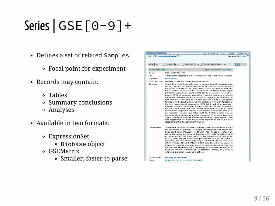
Defines a set of related Samples

Focal point for experiment

Records may contain:

TablesSummary conclusionsAnalyses

Available in two formats:

ExpressionSetBiobase object

GSEMatrixSmaller, faster to parse

Series | GSE[0-9]+

9 / 56

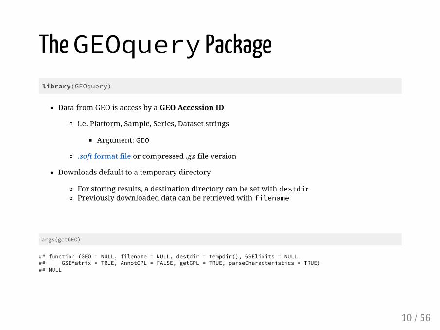
The GEOquery Packagelibrary(GEOquery)

Data from GEO is access by a GEO Accession ID

i.e. Platform, Sample, Series, Dataset strings

Argument: GEO

.soft format file or compressed .gz file version

Downloads default to a temporary directory

For storing results, a destination directory can be set with destdirPreviously downloaded data can be retrieved with filename

args(getGEO)

## function (GEO = NULL, filename = NULL, destdir = tempdir(), GSElimits = NULL, ## GSEMatrix = TRUE, AnnotGPL = FALSE, getGPL = TRUE, parseCharacteristics = TRUE) ## NULL

10 / 56

GEOquery Data StructuresGDS, GPL, and GSM

Class-specific accessor functionsSummary of object structure can be obtained by show()

Comprised of:Metadata headerGeoDataTable

ColumnsTable

GSE

A more heterogeneous containerComposite type from GSM and GPLMay contain data from multiple experiments

i.e. Different platforms, sample setsEach set comprises an ExpressionSet container

11 / 56

## Using locally cached version of GDS1028 found here:## geoData/GDS1028.soft.gz

## Parsed with column specification:## cols(## ID_REF = col_character(),## IDENTIFIER = col_character(),## GSM30361 = col_double(),## GSM30362 = col_double(),## GSM30363 = col_double(),## GSM30364 = col_double(),## GSM30365 = col_double(),## GSM30366 = col_double(),## GSM30367 = col_double(),## GSM30368 = col_double(),## GSM30369 = col_double(),## GSM30370 = col_double(),## GSM30371 = col_double(),## GSM30372 = col_double(),## GSM30373 = col_double(),## GSM30374 = col_double()## )

# Return object size in bytespryr::object_size(gds)

## 2.19 MB

# Object classclass(gds)

## [1] "GDS"## attr(,"package")## [1] "GEOquery"

isS4(gds) # S4 object

## [1] TRUE

GEO DatasetsThe main function for accessing GEO data is getGEO()

gds <- GEOquery::getGEO(GEO = "GDS1028", destdir = "geoData")

12 / 56

GDS MetadataMeta() returns a list of object metadata

GEOquery::Meta(gds)[c("title", "description", "ref", "platform", "platform_technology_type", "sample_organism", "sample_id", "sample_type")]

## $title## [1] "Severe acute respiratory syndrome expression profile"## ## $description## [1] "Expression profiling of peripheral blood mononuclear cells (PBMC) from 10 adult patients with severe acute respirat## [2] "control" ## [3] "SARS" ## ## $ref## [1] "Nucleic Acids Res. 2005 Jan 1;33 Database Issue:D562-6"## ## $platform## [1] "GPL201"## ## $platform_technology_type## [1] "in situ oligonucleotide"## ## $sample_organism## [1] "Homo sapiens"## ## $sample_id## [1] "GSM30361,GSM30362,GSM30363,GSM30364" ## [2] "GSM30365,GSM30366,GSM30367,GSM30368,GSM30369,GSM30370,GSM30371,GSM30372,GSM30373,GSM30374"## ## $sample_type## [1] "RNA"

13 / 56

GDS ColumnsColumns() returns a data.frame of column descriptors

Includes information about each of the samples including in the data

GEOquery::Columns(gds) %>% tibble::as_tibble()

## # A tibble: 14 x 3## sample disease.state description ## <fct> <fct> <chr> ## 1 GSM30361 control Value for GSM30361: N1; src: PBMC normal sample RNA ## 2 GSM30362 control Value for GSM30362: N2; src: PBMC normal sample RNA ## 3 GSM30363 control Value for GSM30363: N3; src: PBMC normal sample RNA f…## 4 GSM30364 control Value for GSM30364: N4; src: PBMC normal sample RNA f…## 5 GSM30365 SARS Value for GSM30365: S1; src: SARS patient blood sample## 6 GSM30366 SARS Value for GSM30366: S2; src: SARS patient blood sample## 7 GSM30367 SARS Value for GSM30367: S3; src: SARS patient blood sample## 8 GSM30368 SARS Value for GSM30368: S4; src: SARS patient blood sample## 9 GSM30369 SARS Value for GSM30369: S5; src: SARS patient blood sample## 10 GSM30370 SARS Value for GSM30370: S6; src: SARS patient blood sample## 11 GSM30371 SARS Value for GSM30371: S7; src: SARS patient blood sample## 12 GSM30372 SARS Value for GSM30372: S8; src: SARS patient blood sample## 13 GSM30373 SARS Value for GSM30373: S9; src: SARS patient blood sample## 14 GSM30374 SARS Value for GSM30374: S10; src: SARS patient blood samp…

14 / 56

GDS TableTable() returns a data.frame of gene expression data

Columns include gene IDs and expression values by Sample

GEOquery::Table(gds) %>% as_tibble()

## # A tibble: 8,793 x 16## ID_REF IDENTIFIER GSM30361 GSM30362 GSM30363 GSM30364 GSM30365 GSM30366## <chr> <chr> <dbl> <dbl> <dbl> <dbl> <dbl> <dbl>## 1 1007_… MIR4640 322. 257. 331 367. 205. 224. ## 2 1053_… RFC2 205. 294. 217. 262. 216. 266. ## 3 117_at HSPA6 539. 367 529 362. 561. 365. ## 4 121_at PAX8 1278. 880. 1032. 1036. 791. 1016. ## 5 1255_… GUCA1A 51.3 44 41.5 26.4 53.5 36.5## 6 1294_… MIR5193 645. 594. 674. 702. 628. 511. ## 7 1316_… THRA 191. 172. 128. 200. 287 202. ## 8 1320_… PTPN21 9.4 5.9 9.6 21.1 16.4 18.2## 9 1431_… CYP2E1 88.7 51.5 96.4 94.1 88.5 15.4## 10 1438_… EPHB3 242. 20.3 38.8 28.4 129. 39.6## # … with 8,783 more rows, and 8 more variables: GSM30367 <dbl>, GSM30368 <dbl>,## # GSM30369 <dbl>, GSM30370 <dbl>, GSM30371 <dbl>, GSM30372 <dbl>,## # GSM30373 <dbl>, GSM30374 <dbl>

15 / 56

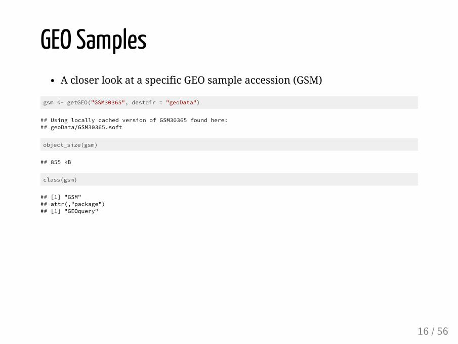
GEO SamplesA closer look at a specific GEO sample accession (GSM)

gsm <- getGEO("GSM30365", destdir = "geoData")

## Using locally cached version of GSM30365 found here:## geoData/GSM30365.soft

object_size(gsm)

## 855 kB

class(gsm)

## [1] "GSM"## attr(,"package")## [1] "GEOquery"

16 / 56

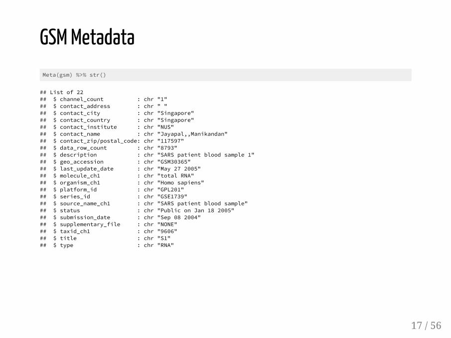
GSM MetadataMeta(gsm) %>% str()

## List of 22## $ channel_count : chr "1"## $ contact_address : chr " "## $ contact_city : chr "Singapore"## $ contact_country : chr "Singapore"## $ contact_institute : chr "NUS"## $ contact_name : chr "Jayapal,,Manikandan"## $ contact_zip/postal_code: chr "117597"## $ data_row_count : chr "8793"## $ description : chr "SARS patient blood sample 1"## $ geo_accession : chr "GSM30365"## $ last_update_date : chr "May 27 2005"## $ molecule_ch1 : chr "total RNA"## $ organism_ch1 : chr "Homo sapiens"## $ platform_id : chr "GPL201"## $ series_id : chr "GSE1739"## $ source_name_ch1 : chr "SARS patient blood sample"## $ status : chr "Public on Jan 18 2005"## $ submission_date : chr "Sep 08 2004"## $ supplementary_file : chr "NONE"## $ taxid_ch1 : chr "9606"## $ title : chr "S1"## $ type : chr "RNA"

17 / 56

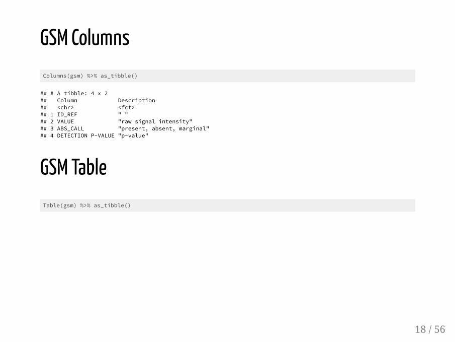
GSM ColumnsColumns(gsm) %>% as_tibble()

## # A tibble: 4 x 2## Column Description ## <chr> <fct> ## 1 ID_REF " " ## 2 VALUE "raw signal intensity" ## 3 ABS_CALL "present, absent, marginal"## 4 DETECTION P-VALUE "p-value"

GSM TableTable(gsm) %>% as_tibble()

18 / 56

GEO Platformsgpl <- getGEO("GPL201", destdir = "geoData")

## Using locally cached version of GPL201 found here:## geoData/GPL201.soft

object_size(gpl)

## 23.9 MB

class(gpl)

## [1] "GPL"## attr(,"package")## [1] "GEOquery"

19 / 56

GEO Platform MetadataMeta(gpl) %>% str(vec.len = 1, nchar.max = 65)

20 / 56

GPL ColumnsColumns(gpl) %>% as_tibble()

## # A tibble: 16 x 2## Column Description ## <chr> <fct> ## 1 ID "Affymetrix Probe Set ID LINK_PRE:\"https://www.affy…## 2 GB_ACC "GenBank Accession Number LINK_PRE:\"http://www.ncbi…## 3 SPOT_ID "identifies controls" ## 4 Species Scientific Name "The genus and species of the organism represented b…## 5 Annotation Date "The date that the annotations for this probe array …## 6 Sequence Type "" ## 7 Sequence Source "The database from which the sequence used to design…## 8 Target Description "" ## 9 Representative Public … "The accession number of a representative sequence. …## 10 Gene Title "Title of Gene represented by the probe set." ## 11 Gene Symbol "A gene symbol, when one is available (from UniGene)…## 12 ENTREZ_GENE_ID "Entrez Gene Database UID LINK_PRE:\"http://www.ncbi…## 13 RefSeq Transcript ID "References to multiple sequences in RefSeq. The fie…## 14 Gene Ontology Biologic… "Gene Ontology Consortium Biological Process derived…## 15 Gene Ontology Cellular… "Gene Ontology Consortium Cellular Component derived…## 16 Gene Ontology Molecula… "Gene Ontology Consortium Molecular Function derived…

21 / 56

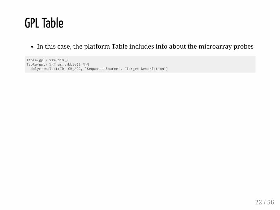
GPL TableIn this case, the platform Table includes info about the microarray probes

Table(gpl) %>% dim()Table(gpl) %>% as_tibble() %>% dplyr::select(ID, GB_ACC, `Sequence Source`, `Target Description`)

22 / 56

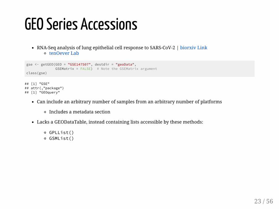
GEO Series AccessionsRNA-Seq analysis of lung epithelial cell response to SARS-CoV-2 | biorxiv Link

tenOever Lab

gse <- getGEO(GEO = "GSE147507", destdir = "geoData", GSEMatrix = FALSE) # Note the GSEMatrix argumentclass(gse)

## [1] "GSE"## attr(,"package")## [1] "GEOquery"

Can include an arbitrary number of samples from an arbitrary number of platforms

Includes a metadata section

Lacks a GEODataTable, instead containing lists accessible by these methods:

GPLList()GSMList()

23 / 56

GSE MetadataMeta(gse)[c("title", "type", "platform_id", "summary", "supplementary_file")]

## $title## [1] "Transcriptional response to SARS-CoV-2 infection"## ## $type## [1] "Expression profiling by high throughput sequencing"## ## $platform_id## [1] "GPL18573" "GPL28369"## ## $summary## [1] "Viral pandemics pose an imminent threat to humanity. The ongoing COVID-19 pandemic, caused ## ## $supplementary_file## [1] "ftp://ftp.ncbi.nlm.nih.gov/geo/series/GSE147nnn/GSE147507/suppl/GSE147507_RawReadCounts_Fer## [2] "ftp://ftp.ncbi.nlm.nih.gov/geo/series/GSE147nnn/GSE147507/suppl/GSE147507_RawReadCounts_Hum

24 / 56

GSMList() and GPLList()GEOquery::GSMList(gse) %>% names()

## [1] "GSM4432378" "GSM4432379" "GSM4432380" "GSM4432381" "GSM4432382"## [6] "GSM4432383" "GSM4432384" "GSM4432385" "GSM4432386" "GSM4432387"## [11] "GSM4432388" "GSM4432389" "GSM4432390" "GSM4432391" "GSM4432392"## [16] "GSM4432393" "GSM4432394" "GSM4432395" "GSM4432396" "GSM4432397"## [21] "GSM4462336" "GSM4462337" "GSM4462338" "GSM4462339" "GSM4462340"## [26] "GSM4462341" "GSM4462342" "GSM4462343" "GSM4462344" "GSM4462345"## [31] "GSM4462346" "GSM4462347" "GSM4462348" "GSM4462349" "GSM4462350"## [36] "GSM4462351" "GSM4462352" "GSM4462353" "GSM4462354" "GSM4462355"## [41] "GSM4462356" "GSM4462357" "GSM4462358" "GSM4462359" "GSM4462360"## [46] "GSM4462361" "GSM4462362" "GSM4462363" "GSM4462364" "GSM4462365"## [51] "GSM4462366" "GSM4462367" "GSM4462368" "GSM4462369" "GSM4462370"## [56] "GSM4462371" "GSM4462372" "GSM4462373" "GSM4462374" "GSM4462375"## [61] "GSM4462376" "GSM4462377" "GSM4462378" "GSM4462379" "GSM4462380"## [66] "GSM4462381" "GSM4462382" "GSM4462383" "GSM4462384" "GSM4462385"## [71] "GSM4462386" "GSM4462387" "GSM4462388" "GSM4462389" "GSM4462390"## [76] "GSM4462391" "GSM4462392" "GSM4462393" "GSM4462394" "GSM4462395"## [81] "GSM4462396" "GSM4462397" "GSM4462398" "GSM4462399" "GSM4462400"## [86] "GSM4462401" "GSM4462402" "GSM4462403" "GSM4462404" "GSM4462405"## [91] "GSM4462406" "GSM4462407" "GSM4462408" "GSM4462409" "GSM4462410"## [96] "GSM4462411" "GSM4462412" "GSM4462413" "GSM4462414" "GSM4462415"## [101] "GSM4462416"

GEOquery::GPLList(gse) %>% names()

## [1] "GPL18573" "GPL28369"

25 / 56

GSM ElementGSMList(gse)[[1]] %>% class()

## [1] "GSM"## attr(,"package")## [1] "GEOquery"

GSMList(gse)[[1]]

## An object of class "GSM"## channel_count ## [1] "1"## characteristics_ch1 ## [1] "cell line: NHBE" ## [2] "cell type: primary human bronchial epithelial cells"## [3] "treatment: Mock treatment" ## [4] "time point: 24hrs after treatment" ## contact_address ## [1] "One Gustave L. Levy Place, Box 1124"## contact_city ## [1] "New York"## contact_country ## [1] "USA"## contact_department ## [1] "Microbiology"## contact_institute ## [1] "Icahn School of Medicine at Mount Sina"## contact_laboratory ## [1] "tenOever Lab"## contact_name ## [1] "Daniel,,Blanco Melo"## contact_state ## [1] "NY"## contact_zip/postal_code ## [1] "10029"## data_processing ## [1] "cDNA libraries were sequenced using an Illumina NextSeq 500 platform" 26 / 56

GPL ElementGPLList(gse)[[1]] %>% class()

## [1] "GPL"## attr(,"package")## [1] "GEOquery"

GPLList(gse)[[1]]

## An object of class "GPL"## contact_country ## [1] "USA"## contact_name ## [1] ",,GEO"## data_row_count ## [1] "0"## distribution ## [1] "virtual"## geo_accession ## [1] "GPL18573"## last_update_date ## [1] "Mar 26 2019"## organism ## [1] "Homo sapiens"## status ## [1] "Public on Apr 15 2014"## submission_date ## [1] "Apr 15 2014"## taxid ## [1] "9606"## technology ## [1] "high-throughput sequencing"## title ## [1] "Illumina NextSeq 500 (Homo sapiens)"## An object of class "GEODataTable"## ****** Column Descriptions ******## [1] Column Description 27 / 56

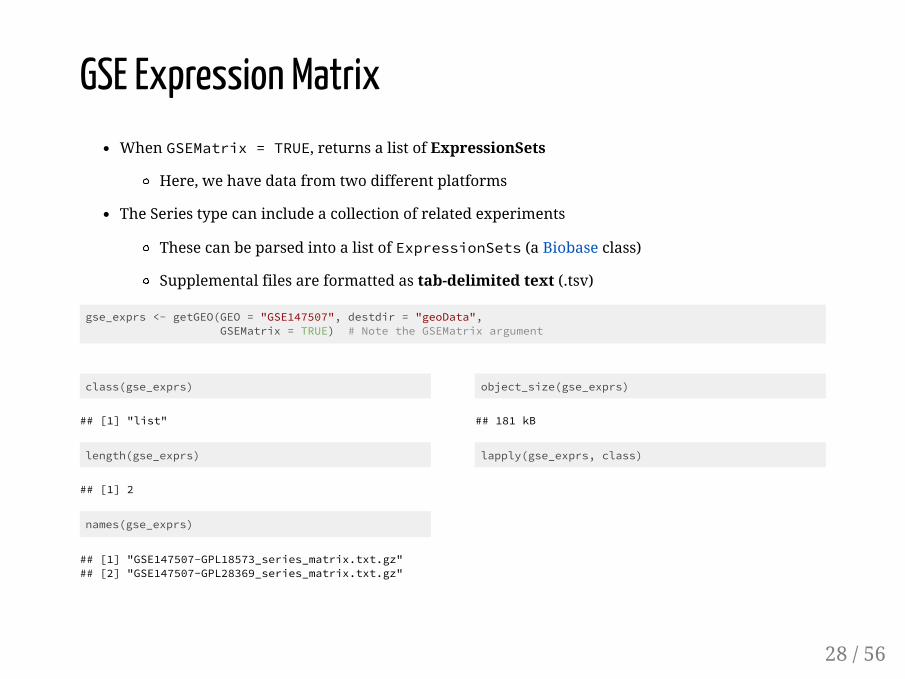
class(gse_exprs)

## [1] "list"

length(gse_exprs)

## [1] 2

names(gse_exprs)

## [1] "GSE147507-GPL18573_series_matrix.txt.gz"## [2] "GSE147507-GPL28369_series_matrix.txt.gz"

object_size(gse_exprs)

## 181 kB

lapply(gse_exprs, class)

GSE Expression MatrixWhen GSEMatrix = TRUE, returns a list of ExpressionSets

Here, we have data from two different platforms

The Series type can include a collection of related experiments

These can be parsed into a list of ExpressionSets (a Biobase class)

Supplemental files are formatted as tab-delimited text (.tsv)

gse_exprs <- getGEO(GEO = "GSE147507", destdir = "geoData", GSEMatrix = TRUE) # Note the GSEMatrix argument

28 / 56

ExpressionSetsThe list can be subset by element name to extract the ExpressionSet

## ExpressionSet (storageMode: lockedEnvironment)## assayData: 0 features, 69 samples ## element names: exprs ## protocolData: none## phenoData## sampleNames: GSM4432378 GSM4432379 ... GSM4462416 (69 total)## varLabels: title geo_accession ... treatment:ch1 (52 total)## varMetadata: labelDescription## featureData: none## experimentData: use 'experimentData(object)'## Annotation: GPL18573

29 / 56

Accessing Phenotype DataExpressionSet objects contain linked phenotype data

Info about tissue / cell type, experiment treatment, methods, etc.

# Extract phenotype data from the ExpressionSetBiobase::pData(gse_GPL18573) %>% as_tibble()

30 / 56

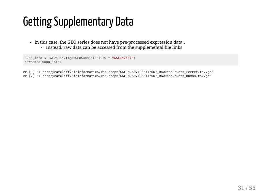
Getting Supplementary DataIn this case, the GEO series does not have pre-processed expression data..

Instead, raw data can be accessed from the supplemental file links

supp_info <- GEOquery::getGEOSuppFiles(GEO = "GSE147507")rownames(supp_info)

## [1] "/Users/jratcliff/Bioinformatics/Workshops/GSE147507/GSE147507_RawReadCounts_Ferret.tsv.gz"## [2] "/Users/jratcliff/Bioinformatics/Workshops/GSE147507/GSE147507_RawReadCounts_Human.tsv.gz"

31 / 56

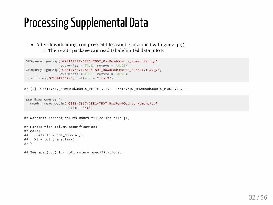
Processing Supplemental DataAfter downloading, compressed files can be unzipped with gunzip()

The readr package can read tab-delimited data into R

GEOquery::gunzip("GSE147507/GSE147507_RawReadCounts_Human.tsv.gz", overwrite = TRUE, remove = FALSE)GEOquery::gunzip("GSE147507/GSE147507_RawReadCounts_Ferret.tsv.gz", overwrite = TRUE, remove = FALSE)list.files("GSE147507/", pattern = ".tsv$")

## [1] "GSE147507_RawReadCounts_Ferret.tsv" "GSE147507_RawReadCounts_Human.tsv"

gse_Hsap_counts <- readr::read_delim("GSE147507/GSE147507_RawReadCounts_Human.tsv", delim = "\t")

## Warning: Missing column names filled in: 'X1' [1]

## Parsed with column specification:## cols(## .default = col_double(),## X1 = col_character()## )

## See spec(...) for full column specifications.

32 / 56

Gene Countsas_tibble(gse_Hsap_counts)

33 / 56

Bioconductor ExpressionSetsThe ALL experiment package contains microarray data

128 patients with acute lymphoblastic leukemia

Here, the data have been pre-processed by RMA normalization

Available as an ExpressionSet object

# BiocManager::install(ALL)library(ALL) # A Bioconductor Experiment Packagedata(ALL) # Load the ExpressionSet object into memory

ALL

## ExpressionSet (storageMode: lockedEnvironment)## assayData: 12625 features, 128 samples ## element names: exprs ## protocolData: none## phenoData## sampleNames: 01005 01010 ... LAL4 (128 total)## varLabels: cod diagnosis ... date last seen (21 total)## varMetadata: labelDescription## featureData: none## experimentData: use 'experimentData(object)'## pubMedIds: 14684422 16243790 ## Annotation: hgu95av2

34 / 56

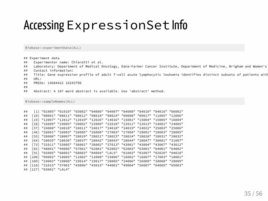
Accessing ExpressionSet InfoBiobase::experimentData(ALL)

## Experiment data## Experimenter name: Chiaretti et al. ## Laboratory: Department of Medical Oncology, Dana-Farber Cancer Institute, Department of Medicine, Brigham and Women's ## Contact information: ## Title: Gene expression profile of adult T-cell acute lymphocytic leukemia identifies distinct subsets of patients with## URL: ## PMIDs: 14684422 16243790 ## ## Abstract: A 187 word abstract is available. Use 'abstract' method.

Biobase::sampleNames(ALL)

## [1] "01005" "01010" "03002" "04006" "04007" "04008" "04010" "04016" "06002"## [10] "08001" "08011" "08012" "08018" "08024" "09008" "09017" "11005" "12006"## [19] "12007" "12012" "12019" "12026" "14016" "15001" "15004" "15005" "16004"## [28] "16009" "19005" "20002" "22009" "22010" "22011" "22013" "24001" "24005"## [37] "24008" "24010" "24011" "24017" "24018" "24019" "24022" "25003" "25006"## [46] "26001" "26003" "26005" "26008" "27003" "27004" "28001" "28003" "28005"## [55] "28006" "28007" "28019" "28021" "28023" "28024" "28028" "28031" "28032"## [64] "28035" "28036" "28037" "28042" "28043" "28044" "28047" "30001" "31007"## [73] "31011" "33005" "36001" "36002" "37013" "43001" "43004" "43007" "43012"## [82] "48001" "49006" "57001" "62001" "62002" "62003" "63001" "64001" "64002"## [91] "65005" "68001" "68003" "84004" "LAL5" "01003" "01007" "02020" "04018"## [100] "09002" "10005" "11002" "12008" "15006" "16002" "16007" "17003" "18001"## [109] "19002" "19008" "19014" "19017" "20005" "24006" "26009" "28008" "28009"## [118] "31015" "37001" "43006" "43015" "44001" "49004" "56007" "64005" "65003"## [127] "83001" "LAL4"

35 / 56

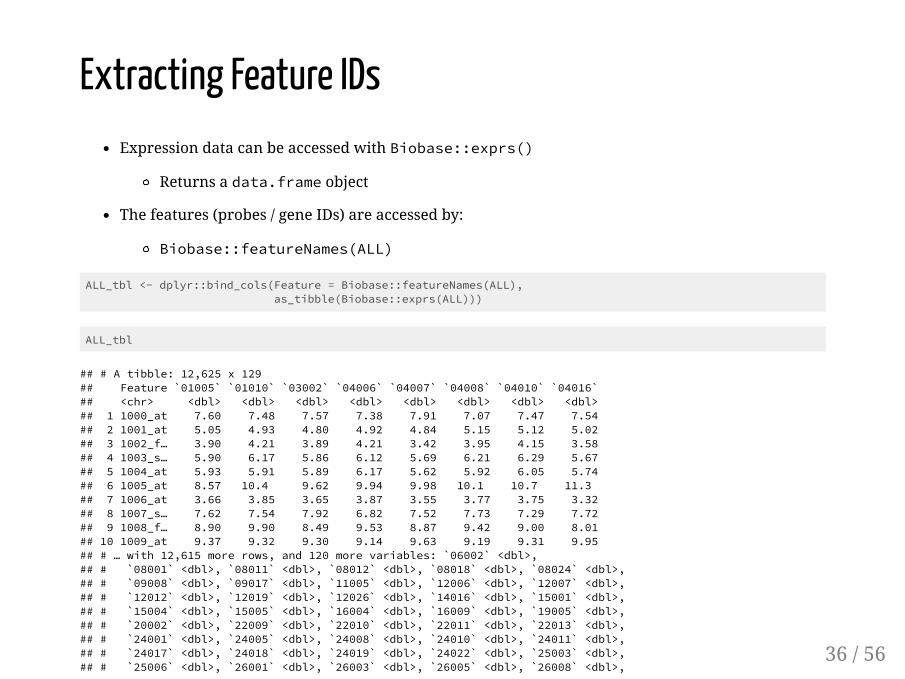
Extracting Feature IDsExpression data can be accessed with Biobase::exprs()

Returns a data.frame object

The features (probes / gene IDs) are accessed by:

Biobase::featureNames(ALL)

ALL_tbl <- dplyr::bind_cols(Feature = Biobase::featureNames(ALL), as_tibble(Biobase::exprs(ALL)))

ALL_tbl

## # A tibble: 12,625 x 129## Feature `01005` `01010` `03002` `04006` `04007` `04008` `04010` `04016`## <chr> <dbl> <dbl> <dbl> <dbl> <dbl> <dbl> <dbl> <dbl>## 1 1000_at 7.60 7.48 7.57 7.38 7.91 7.07 7.47 7.54## 2 1001_at 5.05 4.93 4.80 4.92 4.84 5.15 5.12 5.02## 3 1002_f… 3.90 4.21 3.89 4.21 3.42 3.95 4.15 3.58## 4 1003_s… 5.90 6.17 5.86 6.12 5.69 6.21 6.29 5.67## 5 1004_at 5.93 5.91 5.89 6.17 5.62 5.92 6.05 5.74## 6 1005_at 8.57 10.4 9.62 9.94 9.98 10.1 10.7 11.3 ## 7 1006_at 3.66 3.85 3.65 3.87 3.55 3.77 3.75 3.32## 8 1007_s… 7.62 7.54 7.92 6.82 7.52 7.73 7.29 7.72## 9 1008_f… 8.90 9.90 8.49 9.53 8.87 9.42 9.00 8.01## 10 1009_at 9.37 9.32 9.30 9.14 9.63 9.19 9.31 9.95## # … with 12,615 more rows, and 120 more variables: `06002` <dbl>,## # `08001` <dbl>, `08011` <dbl>, `08012` <dbl>, `08018` <dbl>, `08024` <dbl>,## # `09008` <dbl>, `09017` <dbl>, `11005` <dbl>, `12006` <dbl>, `12007` <dbl>,## # `12012` <dbl>, `12019` <dbl>, `12026` <dbl>, `14016` <dbl>, `15001` <dbl>,## # `15004` <dbl>, `15005` <dbl>, `16004` <dbl>, `16009` <dbl>, `19005` <dbl>,## # `20002` <dbl>, `22009` <dbl>, `22010` <dbl>, `22011` <dbl>, `22013` <dbl>,## # `24001` <dbl>, `24005` <dbl>, `24008` <dbl>, `24010` <dbl>, `24011` <dbl>,## # `24017` <dbl>, `24018` <dbl>, `24019` <dbl>, `24022` <dbl>, `25003` <dbl>,## # `25006` <dbl>, `26001` <dbl>, `26003` <dbl>, `26005` <dbl>, `26008` <dbl>,

36 / 56

Accessing NCBI Databasesrentrez provides functions to programmatically

Leverages the NCBI Eutils API

Programmatic searches of rentrez requires specifying a database

Return a full list of database abbreviations with entrez_dbs()

library(rentrez)rentrez::entrez_dbs() # Vector of accessible NCBI databases

## [1] "pubmed" "protein" "nuccore" "ipg" ## [5] "nucleotide" "structure" "sparcle" "genome" ## [9] "annotinfo" "assembly" "bioproject" "biosample" ## [13] "blastdbinfo" "books" "cdd" "clinvar" ## [17] "gap" "gapplus" "grasp" "dbvar" ## [21] "gene" "gds" "geoprofiles" "homologene" ## [25] "medgen" "mesh" "ncbisearch" "nlmcatalog" ## [29] "omim" "orgtrack" "pmc" "popset" ## [33] "probe" "proteinclusters" "pcassay" "biosystems" ## [37] "pccompound" "pcsubstance" "seqannot" "snp" ## [41] "sra" "taxonomy" "biocollections" "gtr"

37 / 56

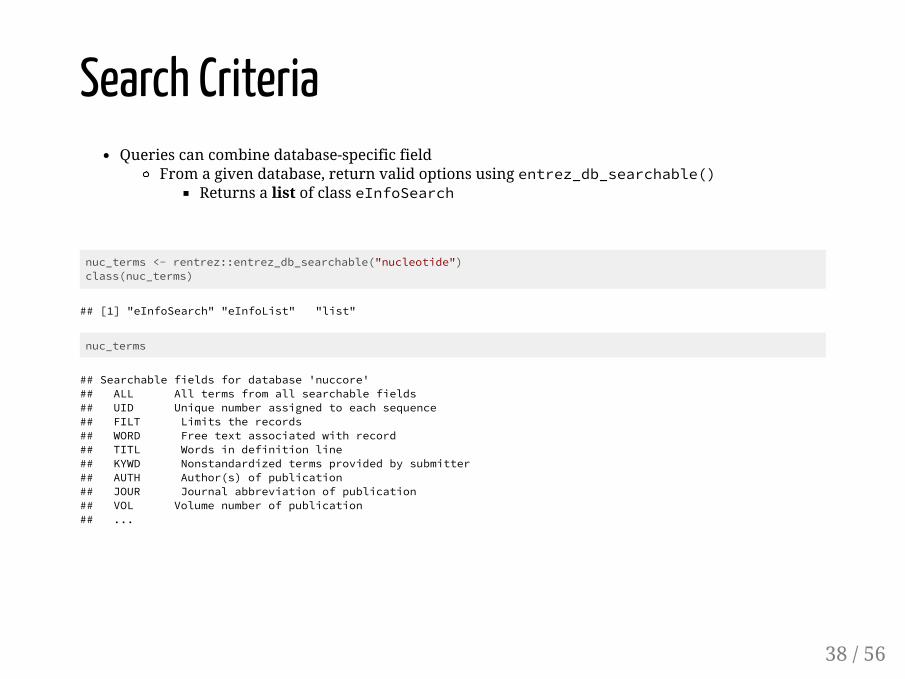
Search CriteriaQueries can combine database-specific field

From a given database, return valid options using entrez_db_searchable()Returns a list of class eInfoSearch

nuc_terms <- rentrez::entrez_db_searchable("nucleotide")class(nuc_terms)

## [1] "eInfoSearch" "eInfoList" "list"

nuc_terms

## Searchable fields for database 'nuccore'## ALL All terms from all searchable fields ## UID Unique number assigned to each sequence ## FILT Limits the records ## WORD Free text associated with record ## TITL Words in definition line ## KYWD Nonstandardized terms provided by submitter ## AUTH Author(s) of publication ## JOUR Journal abbreviation of publication ## VOL Volume number of publication ## ...

38 / 56

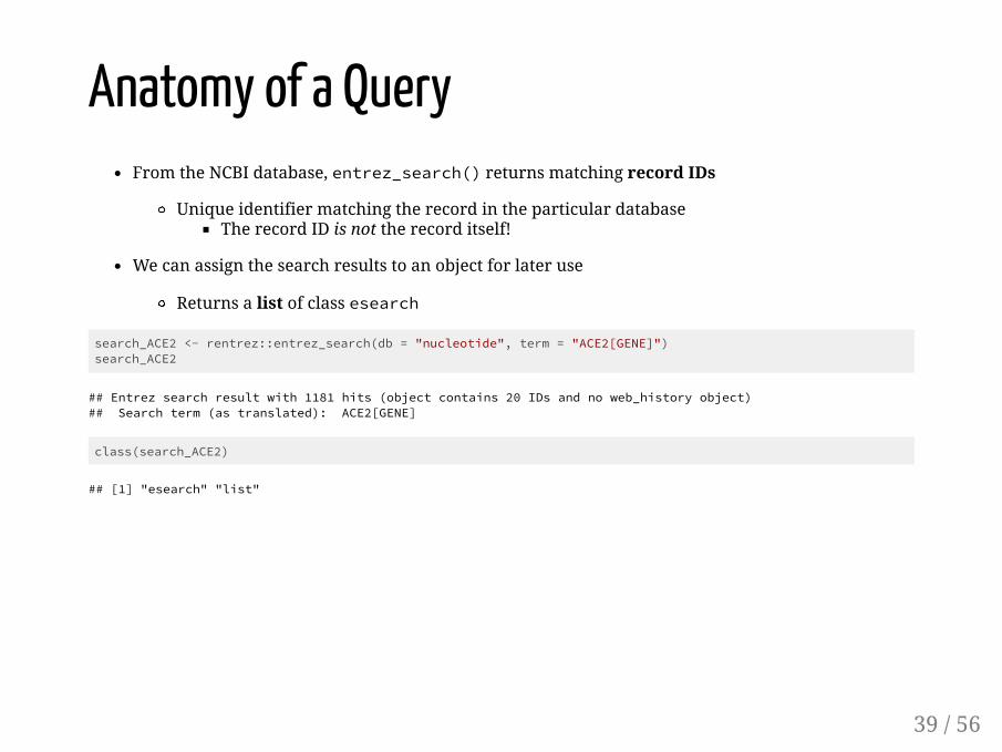
Anatomy of a QueryFrom the NCBI database, entrez_search() returns matching record IDs

Unique identifier matching the record in the particular databaseThe record ID is not the record itself!

We can assign the search results to an object for later use

Returns a list of class esearch

search_ACE2 <- rentrez::entrez_search(db = "nucleotide", term = "ACE2[GENE]")search_ACE2

## Entrez search result with 1181 hits (object contains 20 IDs and no web_history object)## Search term (as translated): ACE2[GENE]

class(search_ACE2)

## [1] "esearch" "list"

39 / 56

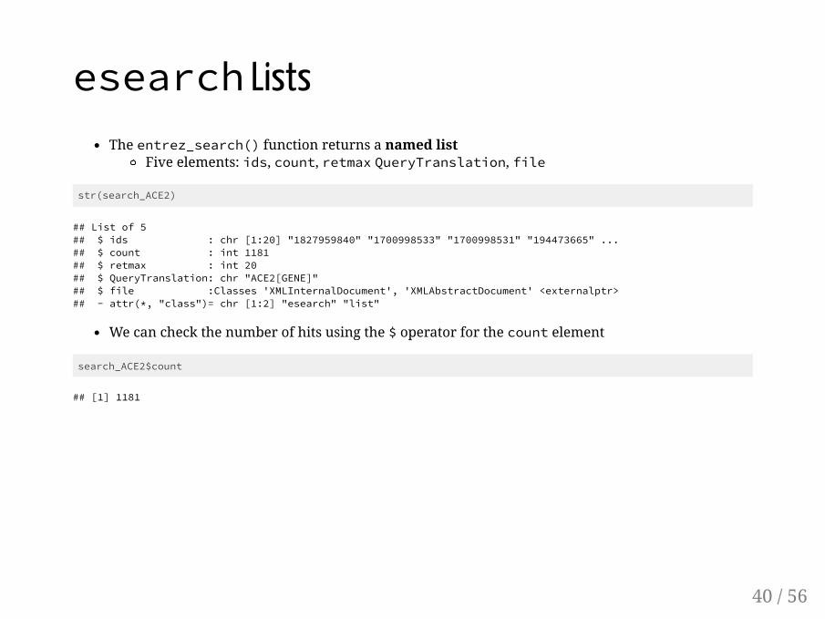
esearch ListsThe entrez_search() function returns a named list

Five elements: ids, count, retmax QueryTranslation, file

str(search_ACE2)

## List of 5## $ ids : chr [1:20] "1827959840" "1700998533" "1700998531" "194473665" ...## $ count : int 1181## $ retmax : int 20## $ QueryTranslation: chr "ACE2[GENE]"## $ file :Classes 'XMLInternalDocument', 'XMLAbstractDocument' <externalptr> ## - attr(*, "class")= chr [1:2] "esearch" "list"

We can check the number of hits using the $ operator for the count element

search_ACE2$count

## [1] 1181

40 / 56

esearch Record IDsElement ids contains our record IDs

The max number of IDs to return is set by the retmax elementDefault value is 20 record identifiers

search_ACE2$ids

## [1] "1827959840" "1700998533" "1700998531" "194473665" "1825945345"## [6] "1823692206" "1820366380" "1728934384" "1823900609" "1822263872"## [11] "1823387078" "1822601922" "1821955509" "1821516010" "1822476874"## [16] "1822437175" "1822437173" "1820171900" "1818868415" "1821009382"

41 / 56

Narrowing a Query1181 hits is a lot of results..

Combining multiple fields allows us to hone our search

Boolean operators (uppercase) AND, OR, NOT can be used

search_ACE2 <- entrez_search(db = "nucleotide", retmax = 157, term = "ACE2[GENE] AND mRNA NOT genome[ALL]")search_ACE2

## Entrez search result with 157 hits (object contains 157 IDs and no web_history object)## Search term (as translated): ACE2[GENE] AND mRNA[All Fields] NOT genome[ALL]

42 / 56

Entrez SummariesThe entrez_summary() function returns a summary record for each UID

It can be helpful to narrow down future searches

search_summary <- rentrez::entrez_summary(db = "nucleotide", id = search_ACE2$id[2])search_summary

## esummary result with 31 items:## [1] uid caption title extra gi ## [6] createdate updatedate flags taxid slen ## [11] biomol moltype topology sourcedb segsetsize ## [16] projectid genome subtype subname assemblygi ## [21] assemblyacc tech completeness geneticcode strand ## [26] organism strain biosample statistics properties ## [31] oslt

search_summary$title

## [1] "Homo sapiens angiotensin I converting enzyme 2 (ACE2), RefSeqGene on chromosome X"

43 / 56

Mapping SummariesNCBI limits requests to 3 per second

This is by default enforced by rentrezTo bump this up to 10/s, register an NCBI API key

See Using API Keys section from the rentrez vignettevignette("rentrez_tutorial", package = "rentrez")

To hone future searches, we can make use of purrr::map()

Here, the search IDs are mapped to return a list of Entrez summariesSubset by title string matching to remove records not of interest

# Map the entrez summaries before fetching records.summary_ace2 <- purrr::map(search_ACE2$ids, function(uid){ entrez_summary(db = "nucleotide", id = uid) })

# Assign vector from substring detection in record titles.# Eliminates case-mismatches from acetylcholinesterase (ace2)detect_ACE2 <- summary_ace2 %>% purrr::map(function(esummary) { stringr::str_detect(string = esummary$title, pattern = "angiotensin I converting enzyme 2")}) %>% unlist()

# Subset by logical vector of string detectionsubset_ace2 <- summary_ace2[detect_ACE2]length(subset_ace2)

## [1] 21

44 / 56

Summary TitlesEach esummary has a title field from the Genbank record

purrr::map_chr(subset_ace2, function(esummary) esummary$title)

## [1] "Homo sapiens angiotensin I converting enzyme 2 (ACE2), transcript variant 2, mRNA" ## [2] "Homo sapiens angiotensin I converting enzyme 2 (ACE2), RefSeqGene on chromosome X" ## [3] "Sus scrofa angiotensin I converting enzyme 2 (ACE2), mRNA" ## [4] "Oryctolagus cuniculus angiotensin I converting enzyme 2 (ACE2) mRNA, complete cds" ## [5] "Rattus norvegicus angiotensin I converting enzyme 2 (Ace2), mRNA" ## [6] "Pongo abelii angiotensin I converting enzyme 2 (ACE2), mRNA" ## [7] "Felis catus angiotensin I converting enzyme 2 (ACE2), mRNA" ## [8] "Macaca mulatta angiotensin I converting enzyme 2 (ACE2), mRNA" ## [9] "Canis lupus familiaris angiotensin I converting enzyme 2 (ACE2), mRNA" ## [10] "Mustela putorius furo angiotensin I converting enzyme 2 (ACE2), mRNA" ## [11] "Pelodiscus sinensis angiotensin I converting enzyme 2 (ACE2) mRNA, partial cds" ## [12] "Capra hircus angiotensin I converting enzyme 2 (ACE2), mRNA" ## [13] "Chinchilla lanigera angiotensin I converting enzyme 2 (Ace2), mRNA" ## [14] "UNVERIFIED: Capra hircus angiotensin I converting enzyme 2-like (ACE2) mRNA, partial sequence"## [15] "Rousettus leschenaultii angiotensin I converting enzyme 2 (ACE2) mRNA, complete cds" ## [16] "Felis catus angiotensin I converting enzyme 2 (ACE2) mRNA, complete cds" ## [17] "Rhinolophus ferrumequinum ACE2 mRNA for angiotensin I converting enzyme 2, complete cds" ## [18] "Rousettus leschenaulti ACE2 mRNA for angiotensin I converting enzyme 2, complete cds" ## [19] "Procyon lotor ACE2 mRNA for angiotensin I converting enzyme 2, complete cds" ## [20] "Felis catus ACE2 mRNA for angiotensin I converting enzyme 2, complete cds" ## [21] "Mustela putorius furo ACE2 mRNA for angiotensin I converting enzyme 2, complete cds"

45 / 56

Fetching ResultsFrom the list of record IDs, we can use entrez_fetch() to get data into R

# Assign vector of unique IDs returned from Entrez summary records.summary_ids <- map_chr(subset_ace2, function(e_summary) e_summary$uid)

# Map fetched NCBI FASTA sequences into a list of DNAString objects.fasta_records <- map(summary_ids, function(summary_id) {

# Fetch FASTA record from NCBI fasta_record <- rentrez::entrez_fetch(db = "nucleotide", id = summary_id, rettype = "FASTA")

# Split FASTA record a fixed number of times to extract sequence header. fasta_split <- stringr::str_split_fixed(fasta_record, pattern = "\n", n = 2) %>% stringr::str_remove_all("\n") # remove additional newline characters

# Build S4 DNAStringSet object from split FASTA record. dna_string_set <- Biostrings::DNAStringSet(x = fasta_split[2]) names(dna_string_set) <- fasta_split[1] dna_string_set})

# Filter out records less than 1kb or greater than 5kbfasta_filtered <- fasta_records %>% purrr::keep(~ BiocGenerics::width(.x) > 1000 & BiocGenerics::width(.x) < 5000)

46 / 56

BioStringsThe BioStrings package defines structures for storing sequence data

Now, we have a list of FASTA sequences as DNAStringSet S4 objects

head(fasta_filtered)

## [[1]]## A DNAStringSet instance of length 1## width seq names ## [1] 3596 GGCACTCATACATACACTCTGGC...ATAAATGCTAGATTTACACACTC >NM_021804.3 Homo...## ## [[2]]## A DNAStringSet instance of length 1## width seq names ## [1] 2418 ATGTCAGGCTCTTTCTGGCTCCT...ATGACATTCAGACTTCGTTTTAG >NM_001123070.1 S...## ## [[3]]## A DNAStringSet instance of length 1## width seq names ## [1] 2435 CAGGATCCATGTCAGGTTCTTCC...AGACTTCATTTTAGGAGCTCCAC >MN099288.1 Oryct...## ## [[4]]## A DNAStringSet instance of length 1## width seq names ## [1] 2418 ATGTCAAGCTCCTGCTGGCTCCT...ATGATGCTCAAACTTCATTCTAA >NM_001012006.1 R...## ## [[5]]## A DNAStringSet instance of length 1## width seq names ## [1] 3668 AGTCTAGGGAAAGTCATTCAGTG...ATATTAACAAAAAAAAAAAAAAA >NM_001131132.2 P...## ## [[6]]## A DNAStringSet instance of length 1## width seq names ## [1] 2510 AAAAACTCATGAAGAGGTTTTAC...GGAAAATCTATTTCCTCTTGAGG >NM_001039456.1 F...

47 / 56

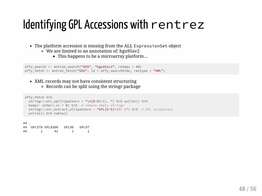
Identifying GPL Accessions with rentrezThe platform accession is missing from the ALL ExpressionSet object

We are limited to an annotation of: hgu95av2This happens to be a microarray platform...

affy_search <- entrez_search("GDS", "hgu95av2", retmax = 44)affy_fetch <- entrez_fetch("GDS", id = affy_search$ids, rettype = "XML")

XML records may not have consistent structuringRecords can be split using the stringr package

affy_fetch %>% stringr::str_split(pattern = "\n[0-9]+\\. ") %>% unlist() %>% keep(~ nchar(.x) > 0) %>% # remove empty strings stringr::str_extract_all(pattern = "GPL[0-9]+(?= )") %>% # GPL accessions unlist() %>% table()

## .## GPL570 GPL8300 GPL96 GPL97 ## 1 42 1 1

48 / 56

Platform Probe IDsaffy_geo <- getGEO("GPL8300", destdir = "geoData")

## Using locally cached version of GPL8300 found here:## geoData/GPL8300.soft

Table(affy_geo) %>% as_tibble()

## # A tibble: 12,625 x 16## ID GB_ACC SPOT_ID `Species Scient… `Annotation Dat… `Sequence Type`## <chr> <chr> <chr> <chr> <chr> <chr> ## 1 1000… X60188 "" Homo sapiens Oct 6, 2014 Exemplar seque…## 2 1001… X60957 "" Homo sapiens Oct 6, 2014 Exemplar seque…## 3 1002… X65962 "" Homo sapiens Oct 6, 2014 Exemplar seque…## 4 1003… X68149 "" Homo sapiens Oct 6, 2014 Exemplar seque…## 5 1004… X68149 "" Homo sapiens Oct 6, 2014 Exemplar seque…## 6 1005… X68277 "" Homo sapiens Oct 6, 2014 Exemplar seque…## 7 1006… X07820 "" Homo sapiens Oct 6, 2014 Exemplar seque…## 8 1007… U48705 "" Homo sapiens Oct 6, 2014 Exemplar seque…## 9 1008… U50648 "" Homo sapiens Oct 6, 2014 Exemplar seque…## 10 1009… U51004 "" Homo sapiens Oct 6, 2014 Exemplar seque…## # … with 12,615 more rows, and 10 more variables: `Sequence Source` <chr>,## # `Target Description` <chr>, `Representative Public ID` <chr>, `Gene## # Title` <chr>, `Gene Symbol` <chr>, ENTREZ_GENE_ID <chr>, `RefSeq Transcript## # ID` <chr>, `Gene Ontology Biological Process` <chr>, `Gene Ontology## # Cellular Component` <chr>, `Gene Ontology Molecular Function` <chr>

49 / 56

Join Gene Symbols# Use `dplyr` to join gene symbols by probe IDGEOquery::Table(affy_geo) %>% dplyr::select(ID, `Gene Symbol`) %>% dplyr::right_join(x = ALL_tbl, by = c("Feature" = "ID")) %>% select(Feature, `Gene Symbol`, dplyr::everything())

## # A tibble: 12,625 x 130## Feature `Gene Symbol` `01005` `01010` `03002` `04006` `04007` `04008` `04010`## <chr> <chr> <dbl> <dbl> <dbl> <dbl> <dbl> <dbl> <dbl>## 1 1000_at MAPK3 7.60 7.48 7.57 7.38 7.91 7.07 7.47## 2 1001_at TIE1 5.05 4.93 4.80 4.92 4.84 5.15 5.12## 3 1002_f… CYP2C19 3.90 4.21 3.89 4.21 3.42 3.95 4.15## 4 1003_s… CXCR5 5.90 6.17 5.86 6.12 5.69 6.21 6.29## 5 1004_at CXCR5 5.93 5.91 5.89 6.17 5.62 5.92 6.05## 6 1005_at DUSP1 8.57 10.4 9.62 9.94 9.98 10.1 10.7 ## 7 1006_at MMP10 3.66 3.85 3.65 3.87 3.55 3.77 3.75## 8 1007_s… DDR1 /// MIR… 7.62 7.54 7.92 6.82 7.52 7.73 7.29## 9 1008_f… EIF2AK2 8.90 9.90 8.49 9.53 8.87 9.42 9.00## 10 1009_at HINT1 9.37 9.32 9.30 9.14 9.63 9.19 9.31## # … with 12,615 more rows, and 121 more variables: `04016` <dbl>,## # `06002` <dbl>, `08001` <dbl>, `08011` <dbl>, `08012` <dbl>, `08018` <dbl>,## # `08024` <dbl>, `09008` <dbl>, `09017` <dbl>, `11005` <dbl>, `12006` <dbl>,## # `12007` <dbl>, `12012` <dbl>, `12019` <dbl>, `12026` <dbl>, `14016` <dbl>,## # `15001` <dbl>, `15004` <dbl>, `15005` <dbl>, `16004` <dbl>, `16009` <dbl>,## # `19005` <dbl>, `20002` <dbl>, `22009` <dbl>, `22010` <dbl>, `22011` <dbl>,## # `22013` <dbl>, `24001` <dbl>, `24005` <dbl>, `24008` <dbl>, `24010` <dbl>,## # `24011` <dbl>, `24017` <dbl>, `24018` <dbl>, `24019` <dbl>, `24022` <dbl>,## # `25003` <dbl>, `25006` <dbl>, `26001` <dbl>, `26003` <dbl>, `26005` <dbl>,## # `26008` <dbl>, `27003` <dbl>, `27004` <dbl>, `28001` <dbl>, `28003` <dbl>,## # `28005` <dbl>, `28006` <dbl>, `28007` <dbl>, `28019` <dbl>, `28021` <dbl>,## # `28023` <dbl>, `28024` <dbl>, `28028` <dbl>, `28031` <dbl>, `28032` <dbl>,## # `28035` <dbl>, `28036` <dbl>, `28037` <dbl>, `28042` <dbl>, `28043` <dbl>,## # `28044` <dbl>, `28047` <dbl>, `30001` <dbl>, `31007` <dbl>, `31011` <dbl>,## # `33005` <dbl>, `36001` <dbl>, `36002` <dbl>, `37013` <dbl>, `43001` <dbl>,## # `43004` <dbl>, `43007` <dbl>, `43012` <dbl>, `48001` <dbl>, `49006` <dbl>,## # `57001` <dbl>, `62001` <dbl>, `62002` <dbl>, `62003` <dbl>, `63001` <dbl>,## # `64001` <dbl>, `64002` <dbl>, `65005` <dbl>, `68001` <dbl>, `68003` <dbl>, 50 / 56

Accessing ClinVar RecordsA number of other databases are available through rentrez

clinvar_search <- entrez_search("clinvar", "ACE2", retmax = 186)clinvar_summary <- entrez_summary(db = "clinvar", id = clinvar_search$ids[1])clinvar_summary

## esummary result with 17 items:## [1] uid obj_type accession ## [4] accession_version title variation_set ## [7] trait_set supporting_submissions clinical_significance ## [10] record_status gene_sort chr_sort ## [13] location_sort variation_set_name variation_set_id ## [16] genes protein_change

51 / 56

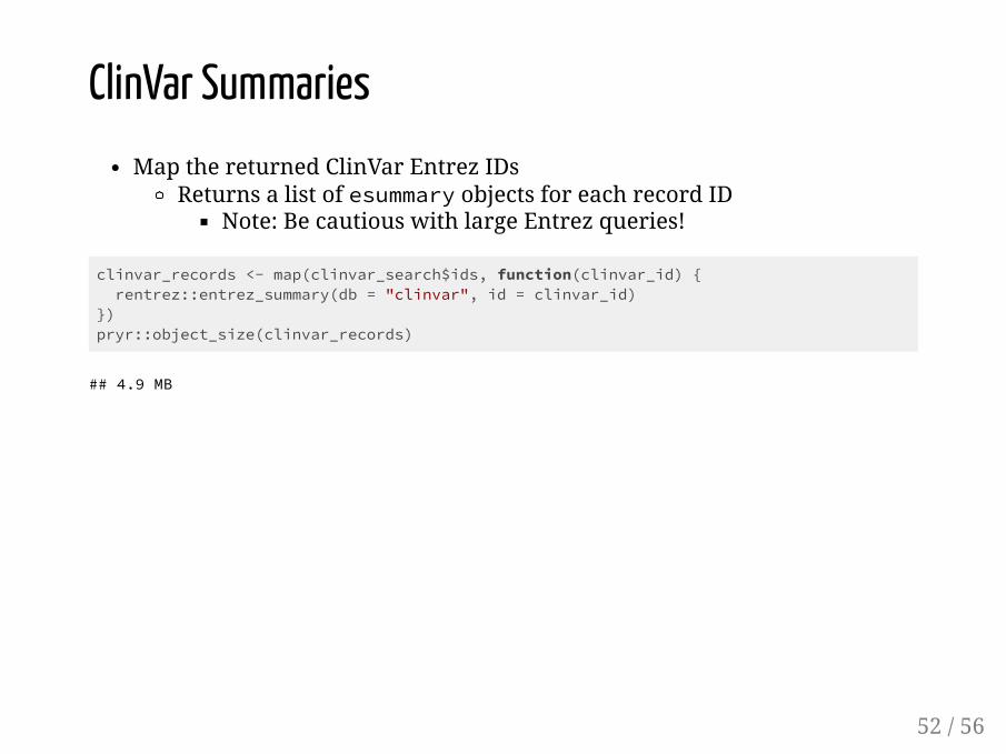
ClinVar SummariesMap the returned ClinVar Entrez IDs

Returns a list of esummary objects for each record IDNote: Be cautious with large Entrez queries!

clinvar_records <- map(clinvar_search$ids, function(clinvar_id) { rentrez::entrez_summary(db = "clinvar", id = clinvar_id)})pryr::object_size(clinvar_records)

## 4.9 MB

52 / 56

Extract Record InformationClinVar summaries provide info on:

Type of variationPathogenicityGenomic location

clinvar_tbl <- clinvar_records %>% purrr::map_dfr(function(cv_sum) { dplyr::bind_cols(unique_id = cv_sum$uid, accession = cv_sum$accession, var_type = cv_sum$obj_type, signif = cv_sum$clinical_significance, var_title = cv_sum$title) })clinvar_tbl %>% select(unique_id, var_type, description, var_title, everything())

## # A tibble: 186 x 7## unique_id var_type description var_title accession last_evaluated## <chr> <chr> <chr> <chr> <chr> <chr> ## 1 816622 copy nu… Pathogenic GRCh37/h… VCV00081… 2018/07/05 00…## 2 816311 copy nu… Uncertain … GRCh37/h… VCV00081… 2018/11/16 00…## 3 816310 copy nu… Uncertain … GRCh37/h… VCV00081… 2019/03/13 00…## 4 816281 copy nu… Pathogenic GRCh37/h… VCV00081… 2018/08/13 00…## 5 816270 copy nu… Pathogenic GRCh37/h… VCV00081… 2018/06/07 00…## 6 816269 copy nu… Pathogenic GRCh37/h… VCV00081… 2018/10/11 00…## 7 816245 copy nu… Pathogenic GRCh37/h… VCV00081… 2019/04/11 00…## 8 780203 single … Likely ben… NM_00137… VCV00078… 2018/08/08 00…## 9 778980 single … Benign NM_00137… VCV00077… 2018/07/30 00…## 10 739305 single … Benign NM_20328… VCV00073… 2018/05/18 00…## # … with 176 more rows, and 1 more variable: review_status <chr>

53 / 56

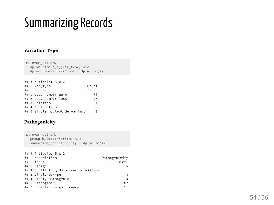
Variation Type

clinvar_tbl %>% dplyr::group_by(var_type) %>% dplyr::summarize(Count = dplyr::n())

## # A tibble: 5 x 2## var_type Count## <chr> <int>## 1 copy number gain 77## 2 copy number loss 98## 3 Deletion 1## 4 Duplication 3## 5 single nucleotide variant 7

Pathogenicity

clinvar_tbl %>% group_by(description) %>% summarize(Pathogenicity = dplyr::n())

## # A tibble: 6 x 2## description Pathogenicity## <chr> <int>## 1 Benign 5## 2 conflicting data from submitters 1## 3 Likely benign 4## 4 Likely pathogenic 3## 5 Pathogenic 162## 6 Uncertain significance 11

Summarizing Records

54 / 56

BiocManager

install()

GEOquery

getGEO()Meta()Columns()Table()GSMList()GPLList()getGEOSuppFiles()gunzip()

Biobase

pData()experimentData()sampleNames()featureNames()

rentrez

entrez_dbs()entrez_db_searchable()entrez_search()entrez_summary()entrez_fetch()

Biostrings

DNAStringSet

BiocGenerics

width()

tibble

as_tibble()

dplyr

select()everything()bind_cols()right_join()group_by()summarize()n()

purrr

map()map_chr()map_dfr()keep()

stringr

str_detect()str_split()str_split_fixed()str_remove_all()str_extract_all()

readr

read_delim()

pryr

object_size()

Package Summary

55 / 56

ReferencesClough E, Barrett T. 2016. The Gene Expression Omnibus Database. In: MathéE, Davis S, editors. Statistical Genomics. Humana Press, New York (NY):Methods in Molecular Biology (vol 1418); 2016. p. 93-110.

56 / 56