
Access to Destinations: Development of Accessibility Measures
125
Access to Destinations: Development of Accessibility Measures Report # 1 in the series Access to Destinations Study Report # 2006-16
Transcript of Access to Destinations: Development of Accessibility Measures
Access to Destinations: Development of Accessibility Measures
Report # 1 in the series Access to Destinations Study
Report # 2006-16

Technical Report Documentation Page1. Report No. 2. 3. Recipients Accession No.
MN/RC-2006-16 4. Title and Subtitle 5. Report Date
Access to Destinations: Development of Accessibility Measures May 2006 6.
7. Author(s) 8. Performing Organization Report No.
Ahmed M. El-Geneidy, David M. Levinson 9. Performing Organization Name and Address 10. Project/Task/Work Unit No.
Department of Civil Engineering University of Minnesota 500 Pillsbury Dr S.E., Room 122 Minneapolis, MN 55455
11. Contract (C) or Grant (G) No.
(c) 81655 (wo)150 12. Sponsoring Organization Name and Address 13. Type of Report and Period Covered
Minnesota Department of Transportation Office of Research Services 395 John Ireland Boulevard Mail Stop 330 St. Paul, Minnesota 55155
Final Report 14. Sponsoring Agency Code
15. Supplementary Notes
http://www.lrrb.org/PDF/200616.pdf Report #1 in the series: Access to Destinations Study 16. Abstract (Limit: 200 words)
Transportation systems are designed to help people participate in activities distributed over space and time. Accessibility indicates the collective performance of land use and transportation systems and determines how well that complex system serves its residents. This research project comprises three main tasks. The first task reviews the literature on accessibility and its performance measures with an emphasis on measures that planners and decision makers can understand and replicate. The second task identifies the appropriate measures of accessibility, where accessibility measures are evaluated in terms of ease of understanding, accuracy and complexity, while the third task illustrates these accessibility measures. During this process a new accessibility measure named “Place Rank” is introduced as an accurate measure of accessibility. In addition, several previously-defined accessibility measures are reviewed and demonstrated in this report including Cumulative opportunity and gravity-based measures. The gravity-based measure is widely used in the literature yet cumulative opportunity tends to be easier to understand and interpret by the public, planners, and administrators. A major contribution of this research is the comparison of accessibility measures over time and among various modes. Effects of accessibility on home sales are also tested. Homebuyers pay a premium to live near jobs and away from competing workers. Accessibility promises to be a useful tool for monitoring the land use and transportation system, and assessing and valuing the benefits of proposed changes to either land use or networks.
17. Document Analysis/Descriptors 18.Availability Statement
Accessibility, Access to Destinations, land use and transportation, place rank, cumulative opportunity, gravity-based
No restrictions. Document available from: National Technical Information Services, Springfield, Virginia 22161
19. Security Class (this report) 20. Security Class (this page) 21. No. of Pages 22. Price
Unclassified Unclassified 125
ACCESS TO DESTINATIONS: DEVELOPMENT OF ACCESSIBILITY
MEASURES
Final Report
Prepared by: Ahmed M. El-Geneidy
David M. Levinson
Networks, Economics, and Urban Systems Research Group Department of Civil Engineering
University of Minnesota
May 2006
Published by: Minnesota Department of Transportation
Research Services Section 395 John Ireland Boulevard, MS 330
St. Paul, MN 55155
This report represents the results of research conducted by the authors and does not necessarily represent the views or policy of the Minnesota Department of Transportation, the Center for Transportation Studies, the Metropolitan Council, and Hennepin County. This report does not contain a standard or specified technique.

ACKNOWLEDGMENT This work was funded by the Minnesota Department of Transportation as part of the Access to Destinations project. The authors would like to thank Mark Filipi, Transportation Forecast/Analyst at the Metropolitan Council, for providing the travel time matrix and other data used in the study. Also thanks are given to Kris Nelson and Jeffrey Matson for providing the LEHD data used in the analysis. Also the authors would like to thank Kevin Krizek and Gavin Poindexter, Humphrey Institute of Public Affairs, for their help in the hedonic analysis. Also, we would like to thank the TAP: James Klessig, Brian Vollum, Deanna Belden, Rabinder Bains, Gina Baas, Mark Filipi, Elizabeth Swift, Gene Hicks, Alan Forsberg and Perry Plank. Finally the authors would like to thank Mohamed Mokbel, Assistant Professor Computer Science Department, University of Minnesota for his help in programming the place rank measure.
TABLE OF CONTENTS
Chapter 1: INTRODUCTION..............................................................................................1
Introduction..................................................................................................................... 1 Definitions....................................................................................................................... 1 Importance ...................................................................................................................... 2 The Need for Accessibility Measures ............................................................................. 3 Study outline ................................................................................................................... 3
Chapter 2: LITERATURE REVIEW.................................................................................. 5 Introduction..................................................................................................................... 5 Network Size................................................................................................................... 5 Cumulative Opportunity Measure................................................................................... 6 Gravity-Based Measure .................................................................................................. 7 Utility-Based Measure .................................................................................................... 8 Constraints-Based Measure ............................................................................................ 9 Composite Accessibility Measure................................................................................... 9 Spatial Comparisons ....................................................................................................... 9 Demand and Accessibility ............................................................................................ 10
Chapter 3: ACCESSIBILITY MEASURES..................................................................... 12 Introduction................................................................................................................... 12 Data ............................................................................................................................... 12 Cumulative Opportunity Measure................................................................................. 14 Gravity-based Measure ................................................................................................. 16 Visualizing Measures of Accessibility.......................................................................... 19
Chapter 4: PLACE RANK – A NEW ACCESSIBILITY MEASURE ............................ 21 Introduction................................................................................................................... 21 Methods......................................................................................................................... 21 Case Study .................................................................................................................... 24 Visual and Statistical Comparison ................................................................................ 27
Chapter 5: EFFECTS OF ACCESSIBILITY ON HOUSE PRICE.................................. 31 Introduction................................................................................................................... 31 Hedonic analysis ........................................................................................................... 31 Data ............................................................................................................................... 31 Statistical Models.......................................................................................................... 34 Discussion..................................................................................................................... 37
Chapter 6: ACCESSIBILITY OVER TIME..................................................................... 38 Introduction................................................................................................................... 38 Methodology and data sources...................................................................................... 38 Detailed Comparative Study ......................................................................................... 39 General Comparative Study.......................................................................................... 41 Changes in Accessibility to Special Destinations......................................................... 47
Chapter 7: CONCLUSIONS............................................................................................. 50 Introduction................................................................................................................... 50 Measures of Accessibility ............................................................................................. 50

Place Rank .................................................................................................................... 50 Applications .................................................................................................................. 51 Measurement Errors...................................................................................................... 51 Effects of Accessibility ................................................................................................. 51 Time Series ................................................................................................................... 51 Future Research ............................................................................................................ 52
REFERENCES 53 APPENDIX A: CUMULATIVE OPPORTUNITY MEASURE AT TAZ LEVEL
MEASURING ACCESS TO JOBS APPENDIX B: CUMULATIVE OPPORTUNITY MEASURE AT TAZ LEVEL
MEASURING ACCESS TO WORKERS APPENDIX C: CUMULATIVE OPPORTUNITY MEASURE AT TAZ LEVEL
MEASURING ACCESS TO RETAIL AND NON-RETAIL JOBS APPENDIX D: ACCESSIBILITY TO RESIDENT WORKERS AT THE MINOR CIVIL
DIVISION LEVEL APPENDIX E: EFFECTS OF ACCESSIBILITY TO RESIDENT WORKERS ON
HOME SALE VALUES AT THE MINOR CIVIL DIVISION LEVEL OF ANALYSIS
APPENDIX F: CUMULATIVE OPPORTUNITY MEASURE AT TAZ LEVEL MEASURING ACCESS TO JOBS OVER TIME USING AUTO AND TRANSIT
APPENDIX G: CUMULATIVE OPPORTUNITY MEASURE AT TAZ LEVEL MEASURING ACCESS TO RESIDENTS OVER TIME USING AUTO AND TRANSIT

LIST OF TABLES Table 1.1: Accessibility Matrix........................................................................................... 3 Table 4.1: Example 1, Calculating place rank original data............................................. 23 Table 4.2: Example 1, Calculating place rank first iteration............................................ 23 Table 4.3: Final Place rank (Rj) For example, 1 .............................................................. 24 Table 4.4: Correlation matrix for place rank and gravity-based accessibility measure ... 29 Table 5.1: Variables included for analysis........................................................................ 32 Table 5.2: Descriptive Statistics ....................................................................................... 33 Table 5.3: Hedonic analysis with accessibility to jobs and resident workers................... 36 Table 6.1: Comparative analysis of cumulative opportunity to jobs ................................ 39 Table 6.2: Comparative analysis of cumulative opportunity to residents......................... 40 Table 6.3: Difference in means test .................................................................................. 40 Table 6.4: Change in the number of people within 20 minutes of special destinations
between the years 2000 and 1990 .................................................................... 49 Table E.1: Hedonic analysis with accessibility to jobs....................................................E-1

LIST OF FIGURES Figure 2.1: Networks to illustrate size ................................................................................ 5 Figure 2.2: The Urban System.......................................................................................... 11 Figure 3.1: Distribution of workers residence and population in the Twin Cities region:
LEHD Dataset (left), US Census Bureau (right).............................................. 13 Figure 3.2: Distribution of the number of jobs in the Twin Cities Region: LEHD Dataset
(left), US Census Bureau (right) ...................................................................... 14 Figure 3.3: Number of jobs within 10 minutes of travel time by automobile during the
morning peak in 2000 ...................................................................................... 15 Figure 3.4: Gravity-based accessibility to jobs by automobile in the Twin Cities region in
2000 using 1/travel time-squared impedance function .................................... 16 Figure 3.5: Gravity-based accessibility to jobs by auto in the Twin Cities region in 2000
using a negative exponential impedance function ........................................... 17 Figure 3.6: Gravity-based accessibility to resident workers in the Twin Cities region
using 1/travel time-squared impedance function ............................................. 18 Figure 3.7: 3D comparison of measures of accessibility to jobs ...................................... 20 Figure 4.1: Place rank mathematical example ................................................................. 22 Figure 4.2: Place rank measure to jobs ............................................................................ 25 Figure 4.3: Cumulative opportunity (number of jobs in 10 minutes by auto in 2000) ..... 26 Figure 4.4: Gravity-based accessibility measure to jobs by auto in 2000 using 1/travel
time-squared impedance function .................................................................... 26 Figure 4.5: 3D Comparison of gravity and place-rank measures of accessibility ............ 28 Figure 4.6: Cumulative opportunities correlated to other measures of accessibility........ 29 Figure 6.1: Selected TAZ for the comparative study........................................................ 39 Figure 6.2: Number of jobs within 15 minutes of travel time in the year 1990 (Auto).... 42 Figure 6.3: Number of jobs within 15 minutes of travel time in the year 2000 (Auto).... 42 Figure 6.4: Number of jobs within 15 minutes of travel time in the year 1990 (Transit). 43 Figure 6.5: Number of jobs within 15 minutes of travel time in the year 2000 (Transit). 43 Figure 6.6: Change in the number of jobs within 15 minutes travel time (2000 – 1990)
(Auto) ............................................................................................................... 44 Figure 6.7: Change in the number of jobs within 15 minutes travel time (2000 – 1990)
(Transit)............................................................................................................ 45 Figure 6.8: Change in the number of people within 15 minutes travel time (2000 – 1990)
(Auto) ............................................................................................................... 46 Figure 6.9: Change in the number of people within 15 minutes travel time (2000 – 1990)
(Transit)............................................................................................................ 47 Figure 6.10: Change in the number of people living within 20 minutes of travel time
between the years 2000 and 1990 (Auto)......................................................... 48 Figure 6.11: Change in the number of people living within 20 minutes of travel time
between the years 2000 and 1990 (Transit) ..................................................... 49 Figure A-1: Number of jobs within 15 minutes of travel time during the morning peak
...................................................................................................................... A-1 Figure A-2: Number of jobs within 20 minutes of travel time during the morning peak.....
........................................................................................................................ A-2
Figure A-3: Number of jobs within 25 minutes of travel time during the morning peak............................................................................................................................. A-3
Figure A-4: Number of jobs within 30 minutes of travel time during the morning peak............................................................................................................................. A-4
Figure A-5: Number of jobs within 35 minutes of travel time during the morning peak............................................................................................................................. A-5
Figure A-6: Number of jobs within 40 minutes of travel time during the morning peak............................................................................................................................. A-6
Figure A-7: Number of jobs within 45 minutes of travel time during the morning peak............................................................................................................................. A-7
Figure A-8: Number of jobs within 50 minutes of travel time during the morning peak............................................................................................................................. A-8
Figure A-9: Number of jobs within 55 minutes of travel time during the morning peak............................................................................................................................. A-9
Figure A-10: Number of jobs within 60 minutes of travel time during the morning peak......................................................................................................................... A-10
Figure B-1: Number of resident workers within 10 minutes of travel time during the morning peak.................................................................................................. B-1
Figure B-2: Number of resident workers within 15 minutes of travel time during the morning peak.................................................................................................. B-2
Figure C-1: Number of retail jobs within 10 minutes of travel time during the morning peak ................................................................................................................ C-1
Figure C-2: Number of non-retail jobs within 10 minutes of travel time during the morning peak.................................................................................................. C-2
Figure C-3: Number of retail jobs within 15 minutes of travel time during the morning peak ................................................................................................................ C-3
Figure C-4: Number of non-retail jobs within 15 minutes of travel time during the morning peak.................................................................................................. C-4
Figure D-1: Place rank measuring accessibility to resident workers ............................. D-1 Figure D-2: Number of resident workers within 10 minutes of travel time during the
morning peak.................................................................................................. D-2 Figure D-3: Gravity-based accessibility to resident workers.......................................... D-3 Figure F-1: Number of jobs within 30 minutes of travel time in the year 1990 (Auto) ..F-1 Figure F-2: Number of jobs within 30 minutes of travel time in the year 2000 (Auto) ..F-2 Figure F-3: Number of jobs within 30 minutes of travel time in the year 1990 (Transit) ....
.........................................................................................................................F-3 Figure F-4: Number of jobs within 30 minutes of travel time in the year 2000 (Transit) ....
.........................................................................................................................F-4 Figure F-5: Number of jobs within 45 minutes of travel time in the year 1990 (Auto) ..F-5 Figure F-6: Number of jobs within 45 minutes of travel time in the year 2000 (Auto) ..F-6 Figure F-7: Number of jobs within 45 minutes of travel time in the year 1990 (Transit) ....
.........................................................................................................................F-7 Figure F-8: Number of jobs within 45 minutes of travel time in the year 2000 (Transit) ....
.........................................................................................................................F-8 Figure F-9: Number of jobs within 60 minutes of travel time in the year 1990 (Auto) ..F-9

Figure F-10: Number of jobs within 60 minutes of travel time in the year 2000 (Auto) ............................................................................................................................F-10
Figure F-11: Number of jobs within 60 minutes of travel time in the year 1990 (Transit) .........................................................................................................................F-11
Figure F-12: Number of jobs within 60 minutes of travel time in the year 2000 (Transit).......................................................................................................................F-12
Figure G-1: Number of people living within 15 minutes of travel time in the year 1990 (Auto) ............................................................................................................. G-1
Figure G-2: Number of people living within 15 minutes of travel time in the year 2000 (Auto) ............................................................................................................. G-2
Figure G-3: Number of people living within 15 minutes of travel time in the year 1990 (Transit).......................................................................................................... G-3
Figure G-4: Number of people living within 15 minutes of travel time in the year 2000 (Transit).......................................................................................................... G-4
Figure G-5: Number of people living within 30 minutes of travel time in the year 1990 (Auto) ............................................................................................................. G-5
Figure G-6: Number of people living within 30 minutes of travel time in the year 2000 (Auto) ............................................................................................................. G-6
Figure G-7: Number of people living within 30 minutes of travel time in the year 1990 (Transit).......................................................................................................... G-7
Figure G-8: Number of people living within 30 minutes of travel time in the year 2000 (Transit).......................................................................................................... G-8
Figure G-9: Number of people living within 45 minutes of travel time in the year 1990 (Auto) ............................................................................................................. G-9
Figure G-10: Number of people living within 45 minutes of travel time in the year 2000 (Auto) ........................................................................................................... G-10
Figure G-11: Number of people living within 45 minutes of travel time in the year 1990 (Transit)........................................................................................................ G-11
Figure G-12: Number of people living within 45 minutes of travel time in the year 2000 (Transit)........................................................................................................ G-12
Figure G-13: Number of people living within 60 minutes of travel time in the year 1990 (Auto) ........................................................................................................... G-13
Figure G-14: Number of people living within 60 minutes of travel time in the year 2000 (Auto) ........................................................................................................... G-14
Figure G-15: Number of people living within 60 minutes of travel time in the year 1990 (Transit)........................................................................................................ G-15
Figure G-16: Number of people living within 60 minutes of travel time in the year 2000 (Transit)........................................................................................................ G-16
EXECUTIVE SUMMARY
Transportation systems are designed to help people participate in activities distributed over space and time. Accessibility indicates the collective performance of land use and transportation systems and determines how well that complex system serves its residents.
The word “accessibility” has been around in the transportation planning field for
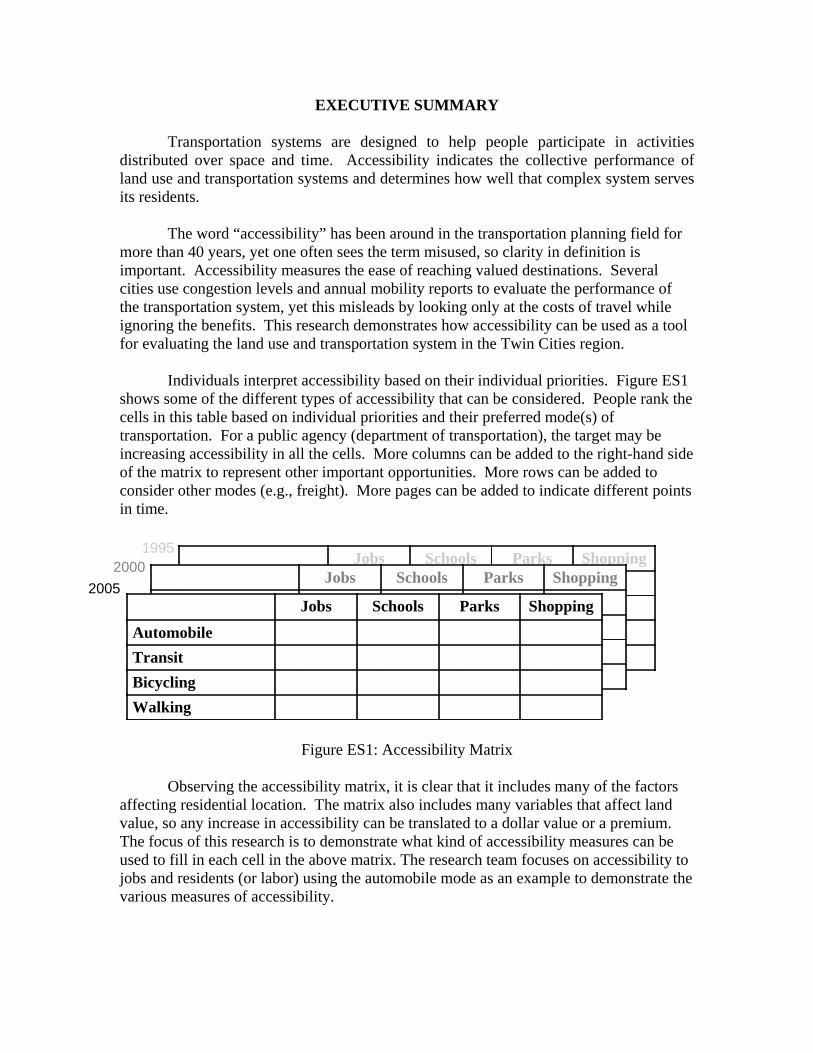
more than 40 years, yet one often sees the term misused, so clarity in definition is important. Accessibility measures the ease of reaching valued destinations. Several cities use congestion levels and annual mobility reports to evaluate the performance of the transportation system, yet this misleads by looking only at the costs of travel while ignoring the benefits. This research demonstrates how accessibility can be used as a tool for evaluating the land use and transportation system in the Twin Cities region. Individuals interpret accessibility based on their individual priorities. Figure ES1 shows some of the different types of accessibility that can be considered. People rank the cells in this table based on individual priorities and their preferred mode(s) of transportation. For a public agency (department of transportation), the target may be increasing accessibility in all the cells. More columns can be added to the right-hand side of the matrix to represent other important opportunities. More rows can be added to consider other modes (e.g., freight). More pages can be added to indicate different points in time.
Figure ES1: Accessibility Matrix
Observing the accessibility matrix, it is clear that it includes many of the factors
affecting residential location. The matrix also includes many variables that affect land value, so any increase in accessibility can be translated to a dollar value or a premium. The focus of this research is to demonstrate what kind of accessibility measures can be used to fill in each cell in the above matrix. The research team focuses on accessibility to jobs and residents (or labor) using the automobile mode as an example to demonstrate the various measures of accessibility.
WalkingBicyclingTransitAutomobile
ShoppingParksSchoolsJobs
WalkingBicyclingTransitAutomobile
ShoppingParksSchoolsJobs
WalkingBicyclingTransitAutomobile
ShoppingParksSchoolsJobs2005
19952000

This research project comprises three main tasks. The first task reviews the literature on accessibility and its performance measures with an emphasis on measures that planners and decision makers can understand and replicate. The second task identifies the appropriate measures of accessibility, where accessibility measures are evaluated in terms of ease of understanding, accuracy and complexity. The third task illustrate these accessibility measures. During this process, a new accessibility measure named “Place Rank” is introduced as an accurate measure of accessibility that can take advantage of the vast amount of origin and destination information that is now available for land use and transportation planners. It is a measure that can be implemented and adopted in other regions without knowing point-to-point travel time. A sample of the place rank measure of accessibility to jobs is demonstrated in the following figure (using the U.S. Census Longitudinal Employer-Household Dynamics dataset).
Figure ES2: Place rank measuring accessibility to jobs
In the place rank measure, the level of accessibility in a zone is determined based
on the number of people coming into this zone to reach an opportunity. Place rank accounts for the number of opportunities that an individual passes over in a zone to reach an opportunity in another zone. As a result, a destination zone has a higher ranking if it is able to attract more workers from zones with high numbers of jobs. The legend included
Data Sources Travel time: Met Council Selection: Mn/DOT GIS Files: US Census 2000

in Figure ES2 reports weighted number of jobs at the minor civil division level of analysis.
In addition, several previously-defined accessibility measures are reviewed and
demonstrated in this report. Cumulative opportunity and gravity-based measures tend to be similar when travel time is less than or equal to 30 minutes. The gravity-based measure is widely used in the literature, yet cumulative opportunity tends to be easier to understand and interpret by planners and higher level administration. A major contribution of this research is the comparison of accessibility measures over time and among various modes. Various accessibility measures are used to generate a longitudinal analysis measuring the changes in accessibility levels in the region. The following figures show accessibility over time using a cumulative opportunity measure for the years 1990 and 2000, while the consecutive figures show the difference between accessibility to jobs and accessibility to residents measured in 1990 and 2000 using 15 minutes of travel time as the base and auto as the mode of transportation. The travel time estimation is obtained from the Metropolitan Council transportation planning model, while the land use data comes from the Bureau of the Census.
Figure ES3: Number of jobs that can be reached within 15 minutes of travel time in the
year 1990 (Auto)
Data Sources Travel time: Met Council Selection: Mn/DOT GIS Files: US Census 2000

Figure ES4: Number of jobs that can be reached within 15 minutes of travel time in the
year 2000 (Auto)
Figure ES5: Change in the number of jobs that can be reached within 15 minutes travel
time (2000 – 1990) (Auto)
Data Sources Travel time: Met Council Selection: Mn/DOT GIS Files: US Census 2000

Figure ES6: Change in the number of people who can be reached within 15 minutes
travel time (2000 – 1990) (Auto)
All of the studied measures of accessibility possess similarities, which are observed using both visual and statistical methods. Effects of accessibility on home sales are also tested to generate a better understanding of the value of accessibility to individual homebuyers. All tested accessibility measures to jobs are found to have a positive and statistically significant effect on home sales, while keeping all other variables affecting home sales at their mean values. On the other hand, all tested measures of accessibility to resident workers (the labor force) show a negative and statistically significant effect on home sales, while keeping all other variables affecting home sales at their mean values. Homebuyers pay a premium to live near jobs and away from competing workers.
Accessibility promises to be a useful tool for monitoring the land use and
transportation system, and assessing and valuing the benefits of proposed changes to either land use or networks. This report proposes to use it in a way that engineers, planners, administrators, decision-makers, and the public can easily understand. Finally the report includes a discussion regarding how accessibility over time can be used to generate a land use and transportation performance measure to help in evaluating these systems both within a metropolitan area and between cities.

Accessibility illustrates clearly the benefits that transportation provides, connecting people with destinations given the travel times on the network, rather than simply focusing on costs (the congestion that people experience when moving along roads).

1
Chapter 1: INTRODUCTION
Introduction Alexander et al. (1977, ¶ 59) want to “Put the magic of the city within the reach of everyone in a metropolitan area.” Alexander and his colleagues seek to create an ideal city or region where everyone can reach all the available opportunities. Transportation systems are designed to help people participate in activities distributed over space and time. Accessibility is a measure or indicator of the performance of transportation systems in serving individuals living in a community.
Definitions The concept of “accessibility” has been coin in the transportation planning field
for more than 40 years. Improving accessibility is a common element in the goals section in almost all transportation plans in the US (Handy, 2002). However, the term accessibility is often misused and confused with other terms such as mobility. In order to have a common language in this report, these terms are defined and introduced in this section.
Mobility measures the ability to move from one place to another (Handy, 1994; Hansen, 1959). For example,, assuming both are part of a connected network, a person who owns a car has a higher level of mobility than one who doesn’t. The word accessibility is derived from the words “access” and “ability”, thus meaning ability to access, where “access” is the act of approaching something. The word is derived from the Latin accedere “to come” or “to arrive.” Here we concern ourselves with ease of reaching destinations or activities rather than ease of traveling along the network itself. One of the first definitions of accessibility in the planning field was suggested by Hansen (1959), who defines accessibility as a measure of potential opportunities for interaction.
High levels of mobility can, but do not necessarily reflect high levels of accessibility. High levels of accessibility can be present with low levels of mobility. The distinction between accessibility and mobility can be illustrated by comparing Manhattan and Manitoba. Travel in Manhattan is slow in terms of distance that can be covered in a given unit of time, yet one can reach many things in that same short time. In contrast, speeds on roads in Manitoba are quite high, but the accessibility is lower because there are fewer things to reach. Thus we say Manhattan has higher accessibility while Manitoba has higher mobility.
Because activities take place over space, accessibility cannot be present without some mobility. Where we see both low levels of mobility coupled with high levels of accessibility, it is due to the presence of desired opportunities within a short distance and time – a high density of activities. An origin and a destination combined with potential activity at the destination and travel time or cost are the main parts of any accessibility measure (Koenig, 1980). For example,, when Murray and Wu (2003) measure accessibility to transit service, they use residential location as origin and bus stops as the destination, where the potential and cost of using the bus service is derived from service frequency and walking distance. From our point of view, bus stops are interim, but not final destinations, though the techniques for measurement may be quite similar. Measures

2
of accessibility are thoroughly discussed in the literature, Handy and Neimeier (1997) provide a comprehensive review of measurements of accessibility in the planning field.
Importance From a linguistic stand point, the reader now understands the difference between
accessibility and mobility. This section highlights the importance of accessibility measures to both the supplier and the user of transportation systems. Every year the Texas Transportation Institute releases an annual ranking of the levels of congestion for major cities in the United States. This measure shows the average amount of delay each resident is subject to by living in a certain city, which is an estimate based on a snapshot of a selected dimension of the city, measuring the ability to move around the city under certain constraints. Congestion is a measure of how movement is constrained by too many users for the capacity of the system. Thus congestion is in many respects the inverse of mobility (though mobility can be low even on an uncongested system if there is insufficient network). For example,, in the year 2003, the most congested regions in the United States were Los Angeles, San Francisco and Washington DC respectively (Schrank & Lomax, 2005). It is clear that the top three regions in the mobility report are not the least desirable regions in the country to live; they are attractive cities to residents in term of work opportunities, variety of land-use patterns, and other aspects of life and are among the largest metropolitan areas. Accordingly using mobility (or congestion) as measure of how well the land-use and transportation system interacts in a region is insufficient. This has been long understood by transportation professionals. The aim of the U.S. Department of Transportation is not just providing fast and safe transportation, it also includes providing accessible and convenient transportation that meets the vital interests of the people and enhances quality of life today and in the future (United States Department of Transportation, 1966). Similarly the Minnesota Department of Transportation (MNDOT) has a mission to: “Improve access to markets, jobs, goods and services and improve mobility by focusing on priority transportation improvements and investments that help Minnesotans travel safer, smarter and more efficiently.” (Minnesota Department of Transportation, 2003) The role of accessibility as a measure of how well Mn/DOT is reaching its mission is clear, since accessibility is a measure of the ease of traveling on networks to reach opportunities (markets, jobs, goods and services). For the public sector (For example,, departments of transportation), accessibility can be used as an indicator of the performance of the land use-transportation systems being deployed in a region. Meanwhile the success of the public sector in delivering transportation goods cannot be measured solely by congestion or levels of mobility. Accessibility levels are important in terms of the quality of life in a region. The public sector balances between maximum density levels and the ease of reaching opportunities. For a department of transportation, the issue is not just constructing roads or removing snow from the streets, it is a matter of providing people with means to reach various opportunities in a region. Many transportation agencies take land use as given and uncontrollable, and so aim to improve mobility to increase accessibility (Levinson & Krizek, 2005). Individuals uniquely perceive accessibility based on their individual priorities in life. For example,, for a professor the increase in accessibility to jobs within a region might not be as important as the increase in the levels of accessibility to open space, since
3
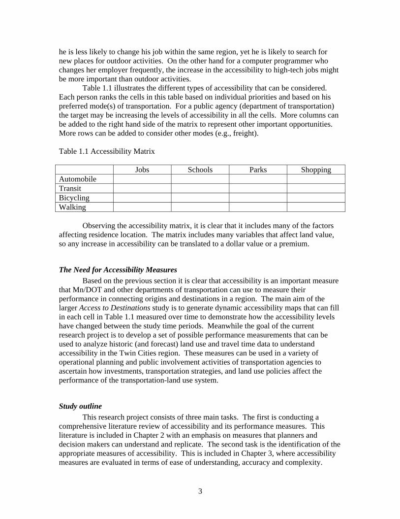
he is less likely to change his job within the same region, yet he is likely to search for new places for outdoor activities. On the other hand for a computer programmer who changes her employer frequently, the increase in the accessibility to high-tech jobs might be more important than outdoor activities. Table 1.1 illustrates the different types of accessibility that can be considered. Each person ranks the cells in this table based on individual priorities and based on his preferred mode(s) of transportation. For a public agency (department of transportation) the target may be increasing the levels of accessibility in all the cells. More columns can be added to the right hand side of the matrix to represent other important opportunities. More rows can be added to consider other modes (e.g., freight). Table 1.1 Accessibility Matrix Jobs Schools Parks Shopping Automobile Transit Bicycling Walking
Observing the accessibility matrix, it is clear that it includes many of the factors affecting residence location. The matrix includes many variables that affect land value, so any increase in accessibility can be translated to a dollar value or a premium.
The Need for Accessibility Measures Based on the previous section it is clear that accessibility is an important measure that Mn/DOT and other departments of transportation can use to measure their performance in connecting origins and destinations in a region. The main aim of the larger Access to Destinations study is to generate dynamic accessibility maps that can fill in each cell in Table 1.1 measured over time to demonstrate how the accessibility levels have changed between the study time periods. Meanwhile the goal of the current research project is to develop a set of possible performance measurements that can be used to analyze historic (and forecast) land use and travel time data to understand accessibility in the Twin Cities region. These measures can be used in a variety of operational planning and public involvement activities of transportation agencies to ascertain how investments, transportation strategies, and land use policies affect the performance of the transportation-land use system.
Study outline This research project consists of three main tasks. The first is conducting a
comprehensive literature review of accessibility and its performance measures. This literature is included in Chapter 2 with an emphasis on measures that planners and decision makers can understand and replicate. The second task is the identification of the appropriate measures of accessibility. This is included in Chapter 3, where accessibility measures are evaluated in terms of ease of understanding, accuracy and complexity.
4
Then a new accessibility measure named “Place Rank” is introduced in Chapter 4. Place rank is a novel and data-intensive measure of accessibility that better accounts for the opportunities people have and choose, which benefits from the vast amount of information that is newly available for land use and transportation planners.
These measures are applied for the Twin Cities region measuring the levels of accessibility based on travel time generated from the Metropolitan Council traffic demand model and utilizing employment data. Accessibility to jobs and to resident workers is used as way to demonstrate the applicability of these measures and the ease of understanding them. Effects of accessibility on home sales are tested in Chapter 5 to generate a better understanding of the value of accessibility to individual homebuyers. Chapter 6 compares estimated accessibility measures over time using previously published data, as well as new calculations for a limited sample of zones. A major contribution of this research is the comparison of accessibility measures over time and among various modes included in this chapter. Various accessibility measures are used to generate a longitudinal analysis measuring the changes in accessibility levels in the region between 1990 and 2000. Finally Chapter 7 outlines how the findings from this project can be used to generate the desired information.
5
Chapter 2: LITERATURE REVIEW
Introduction As was stated earlier, accessibility is a term that has been around for more than 4
decades. Accordingly the literature involving the measurements of accessibility is rich. The traditional measure of accessibility is place-based, and involves measurements of spatial separation of individuals and certain activities. Recently “people-based accessibility” measures have been proposed in the literature (H. Miller, 2005). There are various methods to measure accessibility in a region. For example, (Baradaran & Ramjerdi, 2001) identify five different ways for measuring accessibility, while Handy and Niemeier (1997) used only three of these five as potential measures for planners to use. In this chapter we discuss these measures of accessibility, followed by a discussion relating accessibility measures to changes in land use.
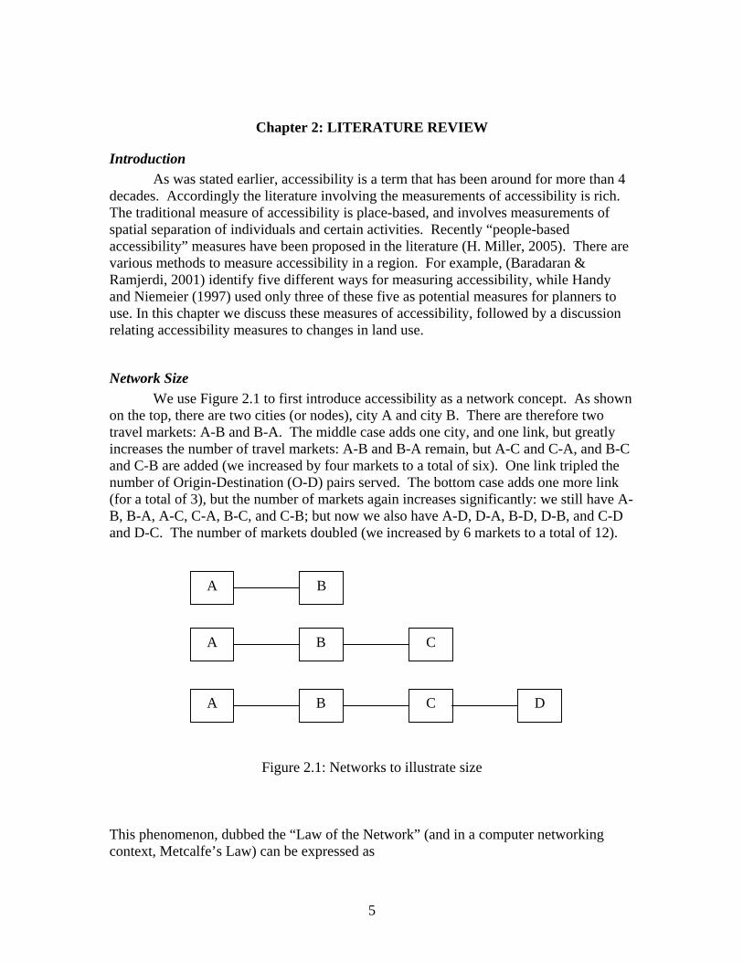
Network Size We use Figure 2.1 to first introduce accessibility as a network concept. As shown
on the top, there are two cities (or nodes), city A and city B. There are therefore two travel markets: A-B and B-A. The middle case adds one city, and one link, but greatly increases the number of travel markets: A-B and B-A remain, but A-C and C-A, and B-C and C-B are added (we increased by four markets to a total of six). One link tripled the number of Origin-Destination (O-D) pairs served. The bottom case adds one more link (for a total of 3), but the number of markets again increases significantly: we still have A-B, B-A, A-C, C-A, B-C, and C-B; but now we also have A-D, D-A, B-D, D-B, and C-D and D-C. The number of markets doubled (we increased by 6 markets to a total of 12).
Figure 2.1: Networks to illustrate size
This phenomenon, dubbed the “Law of the Network” (and in a computer networking context, Metcalfe’s Law) can be expressed as
A B
A C B
A C B D

6
S = N N -1( ) (1)
Where: S = the size of the network (number of markets) N = the number of nodes (To illustrate: with 2 nodes: S = 2*1 = 2, with 3 nodes: S = 3*2 = 6, with 4 nodes: S = 4*3 =12, etc.) The value of S grows non-linearly as nodes are added to the network, until all nodes are connected. Clearly there is increasing value to the network as it gets larger. Since people are willing to pay more for goods of higher value, we would expect that people would pay more to belong to a larger network (live in a larger city). Accessibility (A) differs from Network Size (S), in that accessibility multiplies each interaction by a function of the travel cost, such that far away interactions have less weight than nearby interactions. Accessibility also replaces the simple measure, number of nodes, with a slightly more sophisticated measure, e.g., number of jobs, to measure employment accessibility (or number of workers to measure labor force accessibility). This allows us to see how well the system connects workers with jobs.
Cumulative Opportunity Measure The isochronic or cumulative opportunity measure is one of the basic and early
measures discussed in the literature (Vickerman, 1974; Wachs & Kumagai, 1973). This approach counts the number of potential opportunities that can be reached within a predetermined travel time (or distance).
Ai = Bja j
j=1
J
∑ (2)
Where
iA Accessibility measured at point i to potential activity in zone j
ja Opportunities in zone j
Bj A binary value equals to 1 if zone j is within the predetermined threshold
and 0 otherwise
For instance, this measure can be used to identify the number of recreational opportunities around a residential location i that are within 400 meters (approximately one quarter mile) of network distance (zone j ). This measure does not account for the size of the facility (attractiveness) or the impedance of reaching it (cost). It is widely used in hedonic modeling to control for access to neighborhood amenities. It is simple to understand and calculate, but makes an artificial distinction that opportunities 399 meters away are valuable, while those 401 meters away have no value.

7
Gravity-Based Measure The gravity-based measure discussed in (Hansen, 1959) is still the most widely
used general method for measuring accessibility, although it is more complex in calculations and has some points of weaknesses.
Aim = Oj f (Cijm )
j∑ (3a)
Aim = OjCijm
−2
j∑ (3b)
Aim = Oj exp(θCijm )
j∑ (3c)
Where
Aim Accessibility at point i to potential activity at point j using mode m
Oj The opportunities at point j
)( ijmCf The impedance or cost function to travel between i and j using mode m
exp(θCijm ) Negative exponential function to travel between i and j using mode m
The differences between various studies of accessibility that utilize this method are mainly in functional forms that measure the cost to move between origin and destination and how opportunities are calculated. The opportunities can be the frequency of bus service when measuring accessibility to transit service, while it can be the number of employees when measuring the accessibility to work, or park size when measuring accessibility open space. The accessibility measure is expected to increase with the increase in the opportunity measure. The summation is used so as to include all potential sites j that might encompass desired activities. In other words, if we are measuring accessibility to the Mall of America in the Twin Cities, the total number of individual sites j (denoted with a capital J) will be equal to one since only one Mall of America exists in the Twin Cities. Meanwhile measuring accessibility to shopping malls in the same region will require calculating the previous function to all shopping malls in the region, while using a factor such as number of stores or mall area or retail employees as the potential variable to differentiate between the various shopping mall sizes. This is done using each shopping mall as a destination j then calculating the accessibility variables for each j until we have J (J=total number of destinations) values of accessibility to be summed at the end of the process.
Accessibility is expected to decline the farther the opportunities are from the origin. Much of the literature defines impedance using a negative exponential function. When we say “farther” that can be in terms of time or distance or generalized cost.
The previous equation is applied to measure accessibility using a single transportation mode m. Accessibility can be measured in the same manner for various modes of transportation then a comparison can be conducted. For example,, accessibility to jobs can be measured using automobiles, public transit and bicycling. The findings

8
can then be compared to identify underserved areas or locations that need more attention in terms of accessibility using a certain mode.
Major disadvantages of this accessibility measure are the need to develop an impedance factor (though coefficients from destination choice or trip distribution models already estimated for regional transportation planning models are often used), and the appropriate weights for the destination (e.g., should retail be number of stores, number of retail jobs, or area). Combining the modes is also difficult. One might use one of the following composite measures:
Ai = Oj Mijm
m∑ f (Cijm )
j∑ (4a) or
Ai = Oj f (Cijm )
m∑
j∑ (4b)
where:
Mijm = share of mode m in market ij (0-1) But in (4a) the mode share in a market also depends on the cost of travel, so the
analysis weights travel costs doubly. In (4b), we could introduce a new mode and instantly increase accessibility, even if the new mode was essentially identical to existing modes. One might simply want to say something like this:
Ai = Aim Mim
m∑ (5a) or
Ai = max Aim( ) (5b)
But equations (5a) and (5b) use mode share at the origin, while mode share is a trip (origin and destination-based) phenomenon, so these measures lose information.
Utility-Based Measure The most complex and data intensive is the utility-based measure. Several
researchers use this method since it adheres to travel behavior theories (Ben-Akiva & Lermand, 1977; Neuburger, 1971). The general specification of the measure is as follows:
⎥⎦
⎤⎢⎣
⎡= ∑
∈∀ nCcn
in VA )exp(ln )( (6)
Where
inA Accessibility measured for individual n measure at location i
)(cnV Observable temporal and spatial component of indirect utility of choice c for person n
nC Choice set of person n

9
This measure incorporates individual traveler preferences as part of the
accessibility measure compared to the gravity model where the variation is not present across people living in the same zone. The gravity model implies that all people in zone i will experience the same level of accessibility. In reality people choose destination j he to maximize benefit. This is done through comparing the benefits from going to j1 to the benefit of going to j2.
For example,, suppose we are measuring accessibility to grocery stores. A person n will choose shop c based on prices and other factors like cleanliness of the store. Still other choices are available for this person, who weights going to this one as more valuable than the others. This measure imitates the human choice since the attractiveness of each destination is included. It is based on economic benefits that people derive from having access to certain activities. This measure has several advantages yet its complexity and data intensity are the main barriers to implementing it.
Constraints-Based Measure High levels of accessibility to various activities in a city can be present, yet the
amount of time available in a day that people can spend to reach these activities might not. This leads to the constraints-based measure or people-based measure of accessibility (Wu & Miller, 2002). For example, if a person is at node i at time t1 while at time t2 the same individual has to return to i then the time t = t2 - t1 constrains the number of j destinations available.
Composite Accessibility Measure A fifth measure is the composite accessibility measure. A composite measure is
suggested by (Harvey Miller, 1999) where he combines space-time and utility-based measures in one measure. This approach introduces a higher level of complexity where time constraints are superimposed. The composite accessibility measure requires more data than utility-based measures and it is even more complex in terms of calculations and accordingly generalizing it for usage is not an easy task.
Spatial Comparisons Some measurements of accessibility do not have an easily interpreted meaning at
the zone or parcel level unless they are normalized to determine areas with actual lower levels of accessibility. Normalization can be done in two ways. The first is when accessibility is translated to a dollar value that is often associated with land value. This aspect will be discussed in more detail later in the report. The second aspect is to link accessibility values at a point to general accessibility values in the region. This introduces the aspect of relative accessibility, where accessibility level measured for point i to the potential activity at j , then later in the process the output is divided by the summation of accessibility values measured at all i points around the region.
Normalizing the accessibility to form relative accessibility introduces a measure of equity across the region (Talen, 1998). Relative accessibility is the share of total accessibility that a particular place has. A new transportation facility generally increases absolute accessibility for the region as a whole, we can say it increases the size of the pie.

10
However that facility especially increases the relative accessibility of those places whose residents, workers, or shoppers make use of facility, which is analogous to increasing the percentage of the pie that a particular slice comprises. While society overall has greater accessibility, these markets served by the improvement gain in both absolute and relative accessibility; this implies that other markets may lose relative, if not absolute position. New infrastructure benefits the area around it, but may make other areas worse off, at least in terms of relative position.
There is no right answer when asking which method to use to measure accessibility. The answer depends on what you are trying to measure. If the interest is in city level accessibility, a cumulative opportunity or gravity-based measure will be an option if impedances and attractiveness are well modeled. Relative accessibility can be used to compare neighborhoods. However, if the planner or researcher is more interested in accessibility from an individual perspective, one of the more complex methods mentioned above may be best.
The presence of advanced technologies such as geographic information systems (GIS) and intelligent transportation systems (ITS) introduce, more accurate ways for measuring accessibility. ITS data can provide better utilization, impedance and cost functions for calculations, since travel time and delays can be measured more accurately using such technology. GIS simplifies the city to points of origins and destinations, where potential measurements can be easily conducted. Yet these simplifications need to be conducted carefully, since the underlying calculations in GIS are not usually understood by users (H. Miller & Shaw, 2001). For example, most researchers in accessibility use straight line distances when calculating travel time, or distances from origin to destinations, which is the most common error in accessibility studies. Using distances measured along networks is a more appropriate way, since people generally travel in the city using street or transit networks and not through the air (and even aircraft generally follow fixed paths rather than flying in a straight line).
It is important to note that direct comparison of values or outputs from various measures of accessibility is not appropriate. Since each accessibility measure can be only correlated with itself, normalizations of the measures to relative accessibility are required to conduct such comparison.
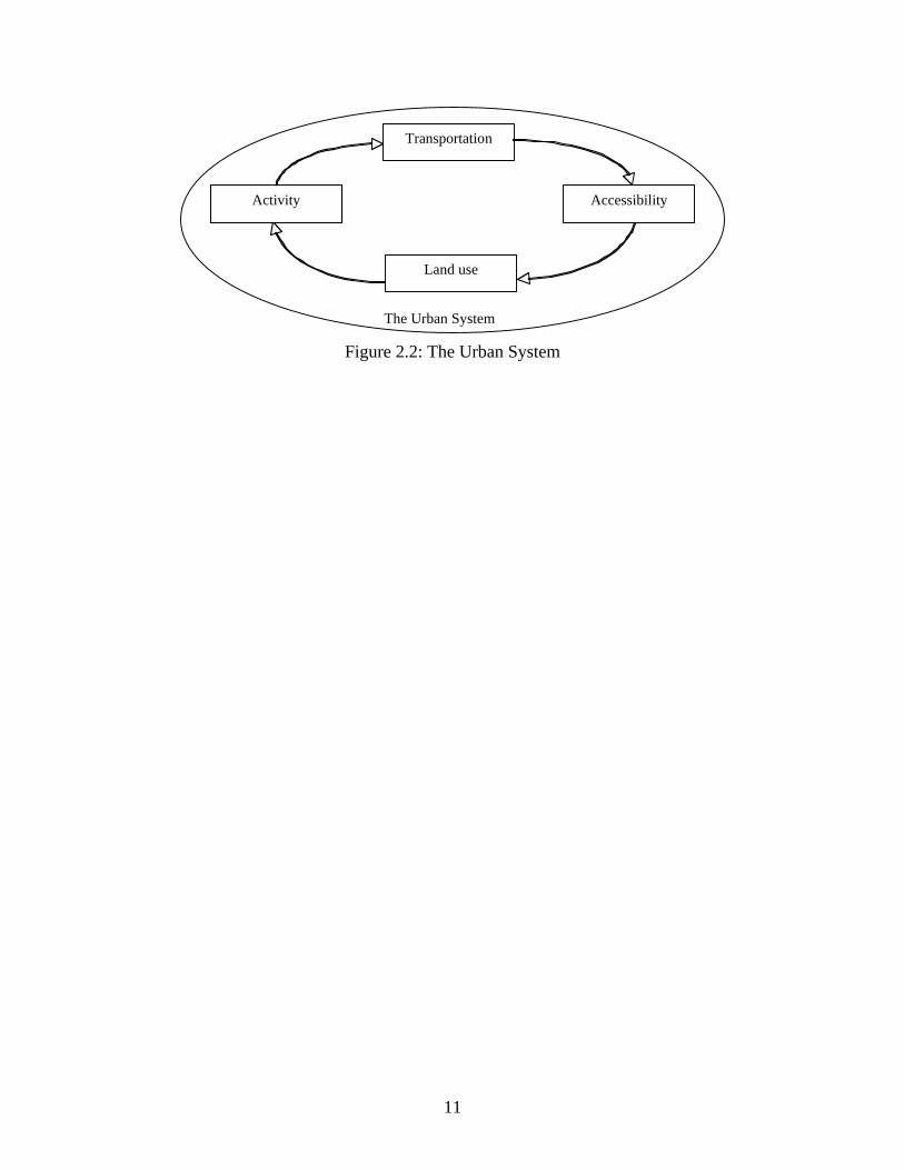
Demand and Accessibility The relationship between land-use, transportation, accessibility, and potential activities can be summarized in the following diagram developed by (Giuliano, 2004), shown in Figure 2.2. Assuming a positive change in the transportation infrastructure or services leads to an increase in accessibility to certain land use in the urban system. These land uses will be experiencing a premium that will eventually lead to a change in the land use patterns and activity. Since the old activity won’t be the ideal usage of land, a change in activity pattern will be present.
11
Transportation
Land use
Accessibility Activity
The Urban System
Figure 2.2: The Urban System

12
Chapter 3: ACCESSIBILITY MEASURES
Introduction All accessibility measures have two major components: the first is the
attractiveness component and the second is the impedance function. The attractiveness component is usually measured as the number of opportunities at destinations. For example, when measuring accessibility to jobs, the attraction value can be the number of jobs at the various potential destinations, while for shopping centers this can be the number of shops in the center. The impedance function decreases the probability of being attracted to such destinations based on distance or travel time. In this report we use accessibility to jobs as our base-case to demonstrate several of the measures discussed in the previous chapter.
The first section of this chapter discusses the available datasets that can be used to generate and demonstrate various accessibility measures. The second section includes a demonstration of the current and most common measures of accessibility used in the transportation planning field (cumulative opportunity measure and gravity-based measure).
Data Measuring accessibility requires knowledge of levels of attractions at destinations
and impedances between those destinations. Impedance can be presented as either distance or travel time or cost between origins and destinations. Travel time is one of the mostly common used functions in the transportation literature. Historically, in transportation planning models the finest disaggregated unit of space that is used for obtaining travel information is at the Transportation Analysis Zone (TAZ). A TAZ is “a geographic area that identifies land uses and associated trips that is used for making land use projections and performing traffic modeling”(American Planning Association, 2005). Travel time is obtained at the TAZ-to-TAZ level of analysis from the transportation planning model of the Metropolitan Council, which is the regional planning agency serving the Twin Cities seven-county metropolitan area. Travel time is available for both congested and uncongested time periods.
For demonstration purposes we measure accessibility to jobs as our base case. The place rank measure, which we discuss in the next chapter, requires knowledge of each worker’s residence and job location. For the cumulative opportunity and gravity-based measures only knowledge of the number of people residing each TAZ and working in it is needed. Origins (residence) and destinations (work location or job site) are available from the U.S. Census Bureau’s Longitudinal Employer-Household Dynamics dataset (LEHD), as processed by the University of Minnesota’s Center for Urban and Regional Analysis (LEHD, 2003). The LEHD is a comprehensive dataset that includes people’s place of residence identified at the Census Block level of analysis and their employment location identified at the same level. In the analysis in this report, the LEHD data is aggregated to the TAZ level of analysis to match the travel time information that was obtained from Metropolitan Council transportation model (Filipi, 2005). In order to compare the various measures of accessibility LEHD data will be used to calculate the

13
opportunities (jobs and resident workers) at origins and destinations for the cumulative opportunity and gravity-based measures. Other data sources also provide similar information about workers, jobs, and population by traffic zone, but only the LEHD links origins and destinations.
Figure 3 shows the number of workers residing each TAZ obtained from the Census Bureau’s LEHD dataset and the number of people living in each TAZ obtained directly from the Census Bureau website (U.S. Census Bureau, 2000). Both datasets are normalized by the total number of people residing the region and the total number of workers in the region. It is clear from the figures that the data track closely.
Figure 3.1: Distribution of workers residence and population in the Twin Cities region: LEHD Dataset (left), US Census Bureau (right)
Figure 3.2 shows the distribution of the normalized number of jobs obtained from the same data sources (LEHD and US Census Bureau). Areas with a high number of jobs are similar in the two maps. To increase the confidence level in the LEHD, a Pearson correlation was tested for the LEHD workers residency and TAZ population. LEHD workers residence is found to be highly correlated to the population residing in a TAZ with a value of 0.96, while the correlation coefficient between the number of jobs obtained from the TAZ and the number of jobs obtained from the LEHD had a value of

14
1.0, which indicates a perfect correlation (which is not surprising since both processed data sets were derived from the same raw Census data). Using LEHD for generating the cumulative opportunity and gravity-based measures of accessibility should lead to the same conclusions if we used Metropolitan Council household or population and jobs by traffic zones or Census datasets.
Figure 3.2: Distribution of the number of jobs in the Twin Cities Region: LEHD Dataset
(left), US Census Bureau (right)
Cumulative Opportunity Measure The isochronic or cumulative opportunity measure counts the number of potential
opportunities that can be reached within a predetermined travel time (or distance). Figure 3.3 shows the cumulative opportunity measure of accessibility to jobs for the Twin Cities metropolitan region measured at 10 minutes of travel time during the morning peak hour from origins.

15
Figure 3.3: Number of jobs within 10 minutes of travel time by automobile during the
morning peak in 2000
Planners and non-professionals can easily interpret this measure. A main point of weakness of the measure is that it does not account for people’s actual choices of residence and employment location. Also, it equally weights people within the same bin of travel time without considering the attractiveness of the areas where they reside or where they are employed. A similar measure can be produced for various time ranges. Appendix A includes a set of Figures showing the cumulative opportunity measure at 15, 20, 25, 30, 35, 40, 45, 50, 55 and 60 minutes of travel time from the origin counting the number of job opportunities within these ranges of travel time using the LEHD dataset. The figures indicate an increase in the number of opportunities with the increase in travel time. Around 70% of the TAZs had more than 1,281,710 jobs within a 50 minute travel time, which indicates the current level of accessibility in the region.
Appendix B includes a set of Figures showing the cumulative opportunity measure at 10 and 15 minutes of travel time from the origin counting the number of resident workers within these ranges of travel time using the LEHD dataset.
Similarly cumulative opportunity measures can be produced for retail and non-retail jobs. Appendix C provides the cumulative opportunity measure for accessibility measured to retail and non-retail jobs in the Twin Cities region using travel time intervals of 10 and 15 minutes of travel time during the morning peak of the year 2000.
Data Sources Travel time: Met Council Transportation Model Employment Data: CURA, University of Minnesota GIS Files: US Census 2000

16
Gravity-based Measure The gravity-based measure developed by Hansen (1959) is still the most widely used general method for measuring accessibility, although it is complex in calculations and has some points of weaknesses. Figure 3.4 shows the Twin Cities metropolitan region with the gravity-based accessibility measured to jobs in the region (following equation 3b). The accessibility levels are shown in shades of color. The unit of analysis used in developing this measure is the TAZs, while using the reciprocal of the square of travel time between each TAZ as the impedance function. The attractiveness of a TAZ is calculated based on the number of jobs reported by the LEHD dataset that was previously used in producing Figure 3.3. The reciprocal of travel time squared, a common and widely used impedance function, is used as the impedance value when calculating this measure of accessibility.
Figure 3.4: Gravity-based accessibility to jobs by automobile in the Twin Cities region in
2000 using 1/travel time-squared impedance function Major disadvantages of this accessibility measure are the need to develop an
impedance factor (though coefficients from destination choice or trip distribution models already estimated for regional transportation planning models are often used), and the appropriate weights for the destination (e.g., should retail be number of stores, number of retail jobs, or area). Combining the modes is also difficult.
Data Sources Travel time: Met Council Transportation Model Employment Data: CURA, University of Minnesota GIS Files: US Census 2000

17
First it is important to note that comparing accessibility measures should be done
in a relative manner and not through comparing numbers directly. It is clear from comparing Figures 3.3 and 3.4 that similarities exist between the two measures of accessibility. TAZs with high levels of accessibility in Figure 3.3 tend to have high numbers of jobs within the 10 minutes travel time range in Figure 3.4. Both maps indicate centralization in the level of accessibility to jobs in the Twin Cities region similar to the centralization observed in the 10 minutes cumulative opportunity measure of accessibility. A statistical analysis conducted later in this report shows the relationship between these measures. It is clear that areas with high levels of accessibility to jobs are located in the area including and surrounding the two major downtowns in the region (Minneapolis and Saint Paul).
Another alternative is to change the impedance function used in generating the gravity-based measure of accessibility. Figure 3.5 shows the level of accessibility to jobs in the Twin Cities region using travel time and an exponential function with θ= -0.1 (following equation 3c) multiplied by the travel time between each TAZ of origin and destination.
Figure 3.5: Gravity-based accessibility to jobs by auto in the Twin Cities region in 2000
using a negative exponential impedance function
Data Sources Travel time: Met Council Transportation Model Employment Data: CURA, University of Minnesota GIS Files: US Census 2000
Data Sources Travel time: Met Council Transportation Model Employment Data: CURA, University of Minnesota GIS Files: US Census 2000
18
Figure 3.5 is similar to Figures 4.6-6.3 which display the cumulative opportunity measure (see Appendix A). The process of selecting the appropriate impedance function is complicated and requires several trials. The reciprocal of travel time squared was the first function used (following Newton’s Laws of Gravity). Some researchers generate various impedance functions and include them as part of a land value analysis to reach the most appropriate measure that is statistically most correlated with land value (and thus how people perceive the effect of transportation on land). This concept is explored later in the report.
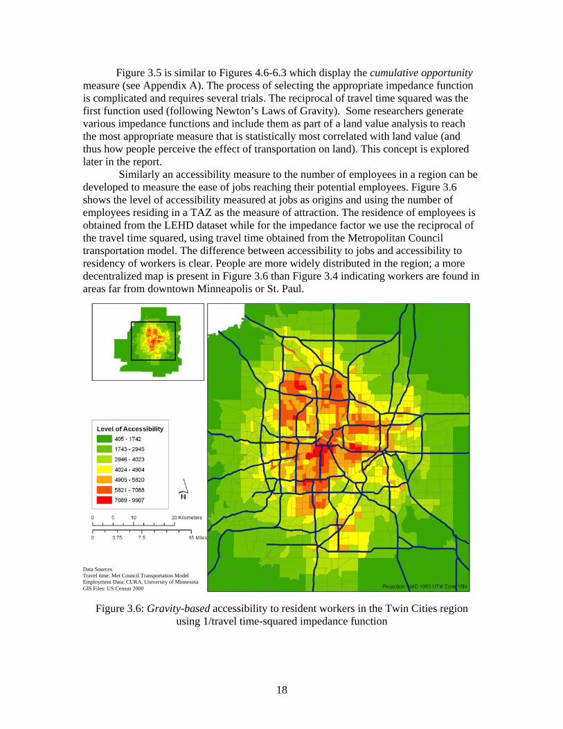
Similarly an accessibility measure to the number of employees in a region can be developed to measure the ease of jobs reaching their potential employees. Figure 3.6 shows the level of accessibility measured at jobs as origins and using the number of employees residing in a TAZ as the measure of attraction. The residence of employees is obtained from the LEHD dataset while for the impedance factor we use the reciprocal of the travel time squared, using travel time obtained from the Metropolitan Council transportation model. The difference between accessibility to jobs and accessibility to residency of workers is clear. People are more widely distributed in the region; a more decentralized map is present in Figure 3.6 than Figure 3.4 indicating workers are found in areas far from downtown Minneapolis or St. Paul.
Figure 3.6: Gravity-based accessibility to resident workers in the Twin Cities region
using 1/travel time-squared impedance function
Data Sources Travel time: Met Council Transportation Model Employment Data: CURA, University of Minnesota GIS Files: US Census 2000

19
Visualizing Measures of Accessibility Linking a gravity-based accessibility measure to jobs and a cumulative
opportunity accessibility measure to jobs within 10 minutes of travel time is possible through utilization of a geographic information system. Figure 3.7 compares the gravity-based and cumulative opportunity measure of accessibility in a three-dimensional format. The first part of the figure (Figure 3.7a) includes the gravity-based accessibility measure to jobs in the Twin Cities region represented in shades of colors and the height are derived from the same measure, while the second part of the figure (Figure 3.7b) shows the cumulative opportunity measure of accessibility to jobs within 10 minutes of travel time from the zone of origin represented in colors and height. Combining the information from both figures is possible in one figure through obtaining the height information from the gravity-based and the color from the cumulative opportunity. This is shown in the third section of the figure (Figure 3.7c). It is clear from Figure 3.7 that areas with high level of accessibility in both measures are similar, but not identical.
It is clear from the figure that a direct relationship exists between both measures of accessibility. This relation will be compared statistically later in this report. For a person familiar with the Twin Cities region observing sections A and C, of the figure can lead him to the idea that these are 3 dimensional maps showing building heights or land values in the region. Downtown Minneapolis and downtown Saint Paul appear to be higher than the rest of the region, while other commercial and suburban areas do show moderate heights.
Figures 3.3 through 3.7 account for the number of opportunities at destinations without weighting the value of the opportunities. The weighting is placed on travel time only, while the attractiveness of each opportunity is weighted based only on the number of opportunities (not the quality of the opportunity or the level of attractiveness of these opportunities). This highlights the need for a measure of accessibility that accounts for the level of attractiveness of a zone based on actual choices.

20
Gravity-based Cumulative opportunity
Gravity-based (Height) and Cumulative opportunity (Color) combined
Figure 3.7: 3D comparison of measures of accessibility to jobs
A
C
B

21
Chapter 4: PLACE RANK – A NEW ACCESSIBILITY MEASURE
Introduction This chapter proposes a new measure of accessibility: “place rank.” Place rank is
an accessibility measure that requires the knowledge of actual choices of origins and destinations. Level of accessibility in a zone is determined based on the number of people coming to this zone to reach an opportunity, where each person contributes to the accessibility level in the zone to which he commutes with a different power. The power of the contribution of this person depends on the attractiveness of his zone of origin. In other words, a destination zone has a higher ranking if it is able to attract more workers from zones with high numbers of jobs. In this chapter we discuss the place ranking measure and compare it to two accessibility measures that are heavily used in the planning literature described in the previous chapter. The first is the isochronic or cumulative opportunity measure and the second is the gravity-based measure.
Methods The place rank measure is inspired from a methodology developed by Brin and
Page (1998) that is used in ranking web pages for large scale search engines, such as Google, which they founded. A web page gets its power from the links connecting to it, while the power of the links comes mainly from the rank of their original host. In an urban planning context this notion can be used to measure the levels of accessibility at destinations and origins. Knowing actual origins and destinations is a key component in this measure of accessibility. The place rank of a zone is determined based on the number of people commuting to this zone to reach an opportunity. The power of the contribution of this person depends on the attractiveness of his zone of origin. The mathematical formulation of the model is as follows:
Rj ,t = Eij * Pit−1i=1
I
∑ (7a)
Pit−1 = [Ej *[Rj ,t−1 / Ei ]] (7b) Where: Rj ,t The place rank of j in iteration t I The total number of i zones that are linked to zone j
ijE The number of people leaving i to reach an activity in j Pit−1 The power of each person leaving i in the previous iteration
jE The original number of people destined for j Ej = Eiji∑
Rj ,t−1 The place ranking of j from the previous iteration
iE The original number of people residing in zone i: Ei = Eijj∑
22
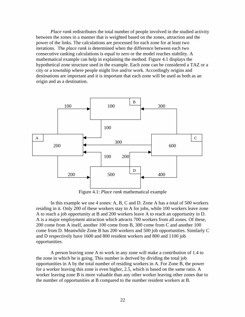
Place rank redistributes the total number of people involved in the studied activity between the zones in a manner that is weighted based on the zones, attraction and the power of the links. The calculations are processed for each zone for at least two iterations. The place rank is determined when the difference between each two consecutive ranking calculations is equal to zero or the model reaches stability. A mathematical example can help in explaining the method. Figure 4.1 displays the hypothetical zone structure used in the example. Each zone can be considered a TAZ or a city or a township where people might live and/or work. Accordingly origins and destinations are important and it is important that each zone will be used as both as an origin and as a destination.
Figure 4.1: Place rank mathematical example In this example we use 4 zones: A, B, C and D. Zone A has a total of 500 workers residing in it. Only 200 of these workers stay in A for jobs, while 100 workers leave zone A to reach a job opportunity at B and 200 workers leave A to reach an opportunity in D. A is a major employment attraction which attracts 700 workers from all zones. Of these, 200 come from A itself, another 100 come from B, 300 come from C and another 100 come from D. Meanwhile Zone B has 200 workers and 500 job opportunities. Similarly C and D respectively have 1600 and 800 resident workers and 800 and 1100 job opportunities. A person leaving zone A to work in any zone will make a contribution of 1.4 to the zone in which he is going. This number is derived by dividing the total job opportunities in A by the total number of residing workers in A. For Zone B, the power for a worker leaving this zone is even higher, 2.5, which is based on the same ratio. A worker leaving zone B is more valuable than any other worker leaving other zones due to the number of opportunities at B compared to the number resident workers at B.
A C
B
D
100 300
400 200
100 200
300
100
200
100
500
600
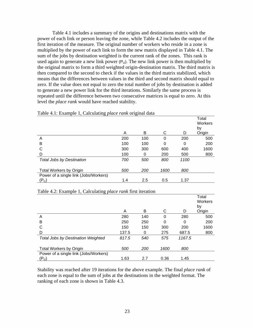
23
Table 4.1 includes a summary of the origins and destinations matrix with the power of each link or person leaving the zone, while Table 4.2 includes the output of the first iteration of the measure. The original number of workers who reside in a zone is multiplied by the power of each link to form the new matrix displayed in Table 4.1. The sum of the jobs by destination weighted is the current rank of the zones. This rank is used again to generate a new link power (Pi2). The new link power is then multiplied by the original matrix to form a third weighted origin-destination matrix. The third matrix is then compared to the second to check if the values in the third matrix stabilized, which means that the differences between values in the third and second matrix should equal to zero. If the value does not equal to zero the total number of jobs by destination is added to generate a new power link for the third iterations. Similarly the same process is repeated until the difference between two consecutive matrices is equal to zero. At this level the place rank would have reached stability. Table 4.1: Example 1, Calculating place rank original data
A B C D
Total Workers by Origin
A 200 100 0 200 500B 100 100 0 0 200C 300 300 600 400 1600D 100 0 200 500 800Total Jobs by Destination 700 500 800 1100 Total Workers by Origin 500 200 1600 800 Power of a single link (Jobs/Workers) (Pi1) 1.4 2.5 0.5 1.37
Table 4.2: Example 1, Calculating place rank first iteration
A B C D
Total Workers by Origin
A 280 140 0 280 500B 250 250 0 0 200C 150 150 300 200 1600D 137.5 0 275 687.5 800Total Jobs by Destination Weighted 817.5 540 575 1167.5 Total Workers by Origin 500 200 1600 800 Power of a single link (Jobs/Workers) (Pi2) 1.63 2.7 0.36 1.45
Stability was reached after 19 iterations for the above example. The final place rank of each zone is equal to the sum of jobs at the destinations in the weighted format. The ranking of each zone is shown in Table 4.3.

24
Table 4.3: Final Place rank (Rj) For example, 1
Zone Place rank A 848.25 B 524.37 C 493.53 D 1233.83
Place rank measures only work when there are both jobs and residents in a
geographic region (otherwise the power of a zone is zero or infinity). Traffic zones are often homogenous, with either many jobs and few or no houses, or many houses and few or no jobs. Thus they cannot be used in place rank measure that requires both incoming and outgoing trips. One needs to look at an area heterogeneous enough to include both jobs and houses. Minor Civil Divisions (MCD) (cities, towns, and townships) in the Twin Cities are one such geography. Alternatively, one could develop a more complex measure, which is not pursued here.
Case Study The place rank measure is applied to the Twin Cities region through aggregating
the LEHD data, which includes origins and destinations of workers resident and employment location. The data was aggregated to the MCD, then the ranking process was developed. Around 300 iterations were needed to reach stability for this model. Figure 4.2 shows the output of the place rank accessibility measure.

25
Figure 4.2: Place rank measure to jobs
It is clear from the figure that concentration of jobs in the heart of the
metropolitan region (the City of Minneapolis) has the highest ranking, while the Cities of Saint Paul, Edina, and Bloomington fall in the second category. These three cities include major headquarters and office buildings such as the Mall of America. Meanwhile, areas in between these cities did show a lower ranking due to the fewer jobs in these areas. For example, a person residing in the city of Minneapolis (the center of the map) and working in the suburbs should be adding more to the ranking of zone where he is working. The reason the city of Minneapolis did show to be at this high ranking level, is not only due to the number of people attracted to the job opportunities in the city, yet it is also due to the strength of the origins where these workers reside.
Comparing the place rank to other accessibility measures is an essential step. Figure 4.3 shows the cumulative accessibility measure showing the number of jobs within 10 minutes of travel time from the origin. This was obtained by aggregating from the TAZ level of analysis to the MCD level for comparison purposes. Figure 4.4 shows the gravity-based accessibility measure to jobs. It is clear that though the three measures show similarities, they are not identical.
Data Sources Employment Data: CURA, University of Minnesota GIS Files: US Census 2000
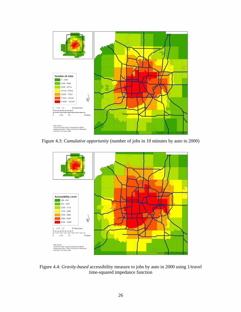
26
Figure 4.3: Cumulative opportunity (number of jobs in 10 minutes by auto in 2000)
Figure 4.4: Gravity-based accessibility measure to jobs by auto in 2000 using 1/travel time-squared impedance function
Data Sources Travel time: Met Council Transportation Model Employment Data: CURA, University of Minnesota GIS Files: US Census 2000
Data Sources Travel time: Met Council Transportation Model Employment Data: CURA, University of Minnesota GIS Files: US Census 2000

27
It is clear from observing Figures 4.3 and 4.4 that the cumulative opportunity measure and gravity-based measure are highly correlated at this level of analysis, but differences exist when comparing these measures to the place rank measure of accessibility. Appendix D compares place rank accessibility to resident workers at the minor civil division level and both the cumulative opportunity measure (number of resident workers within 10 minutes of travel time from the origin) and gravity-based measure (using the inverse of travel time square to generate the impedance function). While the cumulative opportunity measure and gravity-based measure are highly correlated at this level of analysis, place rank is not as highly correlated.
Visual and Statistical Comparison An image is worth a thousand words, so 3-D visualization is used Figure 4.5. The figure combines place rank and the gravity-based measures of accessibility in 3-D that can help in generating a visual comparison. The first part of the figure (Figure 4.5a) shows the gravity based measure conducted at the MCD level of analysis with both color and height representing the accessibility measure using gravity based. The second part of the figure (Figure 4.5b) includes a 3-D representation of the MCDs with place rank in both color and height. Finally the third part of the figure (Figure 4.5c) shows the combination of the two measures where place rank is represented in shades of colors and the height is derived from the gravity-based measure of accessibility. It is clear that some kinds of relationships do exist between place rank accessibility measures and other measures of accessibility. The place rank accessibility measure is also conducted to measure accessibility to resident workers measured from job destinations. The maps of this example are included in Appendix D.

28
Gravity-based Place rank
Gravity-based (Height) and Place rank (Color) combined
Figure 4.5: 3D Comparison of gravity and place-rank measures of accessibility
From a statistical standpoint, a correlation matrix can be generated to compare the three measures of accessibility. The correlation matrix was constructed using the Pearson’s measure of correlation and is shown in Table 4.4.
A
C
B

29
Table 4.4: Correlation matrix for place rank and gravity-based accessibility measure
Place rank to resident
workers
Place rank to
jobs
Gravity-based measure to
jobs
Gravity-based resident workers
Place rank to resident workers 1.000 Place rank to jobs 0.752 1.000 Gravity-based measure to jobs 0.431 0.572 1.000 Gravity-based resident workers 0.425 0.415 0.944 1.000
Place rank to jobs is highly correlated to place rank to resident workers, (even more, the gravity-based measure of accessibility to jobs is highly correlated with accessibility to resident workers). Accessibility to jobs measured used the place rank method shows a medium correlation to the gravity-based measure of accessibility.
0
0.1
0.2
0.3
0.4
0.5
0.6
0.7
0.8
0.9
1
10 20 30 40 50 60
Cumulative Opportunities Measure (Time Bins in Minutes)
Corr
elat
ion
Valu
e
Place Rank (Jobs)Gravity Based (Jobs)Place Rank (Resident Workers)Gravity Based (Resident Workers)
Figure 4.6: Cumulative opportunities correlated to other measures of accessibility Figure 4.6 shows the level of correlation between the gravity-based measure and place rank measures of accessibility to jobs and resident workers to various cumulative opportunity measures. The cumulative opportunity measure is calculated either based on the number of jobs or resident workers that can be reached within 10, 15, 20, 30, 40, 45, 50 and 60 minutes of travel time. The gravity-based method is highly correlated to the cumulative accessibility measure at the 10, 15, 20 and 30 minutes bins. This relation tends to decline with the increase in the travel time bin (40, 45, 50 and 60). Place rank is

30
less correlated to the cumulative opportunity measure than the gravity-based method. In addition, a decline in the level of correlation is present at the higher level bins (40, 45, 50 and 60). The same phenomenon is present for the resident workers place rank measure.

31
Chapter 5: EFFECTS OF ACCESSIBILITY ON HOUSE PRICE
Introduction In this chapter we examine the connection between single-family residence
property values and accessibility to jobs and resident workers in the Twin Cities metropolitan region. This section of the study is conducted to illustrate the effects of accessibility on home sale prices in the region. All three accessibility measures (gravity-based, cumulative opportunity, and place rank) are tested against sale prices of single family houses.
Hedonic analysis In a recent study, accessibility to jobs measured at the parcel level did show it to
have a positive impact on land value (Srour et al., 2002). This highlights the importance of accessibility to the individual, even though each person usually holds only one job at a time. Similarly Franklin and Waddell (2003) noticed a positive effect of accessibility measures to certain jobs in King County, Washington. Both studies show that benefits of accessibility can be capitalized into housing prices. A recent comprehensive review of the literature related to hedonic analysis is conducted by Sirmans and Macpherson (2003), who documented around 200 applications that have examined home sales to estimate values of several home attributes including structural features (e.g.,, lot size, finished square feet, and number of bedrooms), internal and external features (e.g.,, fireplaces, air conditioning, garage spaces, and porches), natural environment features (e.g.,, scenic views), attributes of the neighborhood and location (e.g.,, crime, golf courses, and trees), public services (e.g.,, school and infrastructure quality), marketing, and financing.
Other researchers included accessibility measures to their models as a way to increase the explanatory power of the hedonic models (Franklin & Waddell, 2003; Srour et al., 2002). They included accessibility to jobs, school quality, and measures of environmental amenities. After reviewing several research papers related to the topic of hedonic analysis, the factors affecting single family sales can be summarized into building and lot characteristics, community characteristics, neighborhood characteristics, and accessibility measures.
Data Home sale records for the year 2004 were obtained from the Minnesota Multiple
Listing Service database (MLS). MLS is a realtors association that gathers data from home sales from multiple realtors in the Twin Cities region. MLS data includes detailed information related to the house that is being sold. This information includes the number of bedrooms, number of bathrooms, presence of a fire place, number of garage stalls, lot size, single family house ownership information (previously owned, new building, and under construction), information related to associations that the sold building is related to, and building foot print. Since this database is maintained for the Twin Cities region, which is a region well known for the lakes and ponds, a view variable is included to define if a view to one of the lakes or ponds exists. Accordingly such a comprehensive dataset can be used for generating information related to the building and lot
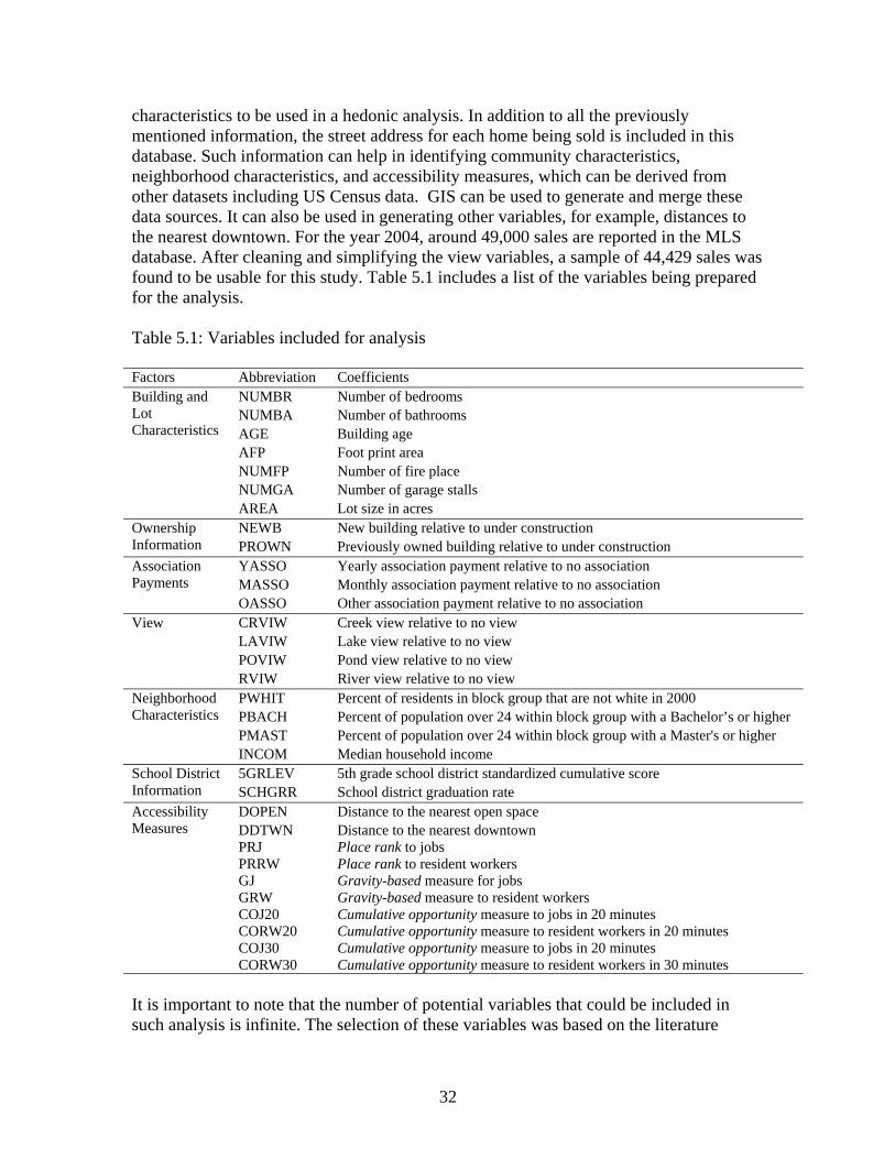
32
characteristics to be used in a hedonic analysis. In addition to all the previously mentioned information, the street address for each home being sold is included in this database. Such information can help in identifying community characteristics, neighborhood characteristics, and accessibility measures, which can be derived from other datasets including US Census data. GIS can be used to generate and merge these data sources. It can also be used in generating other variables, for example, distances to the nearest downtown. For the year 2004, around 49,000 sales are reported in the MLS database. After cleaning and simplifying the view variables, a sample of 44,429 sales was found to be usable for this study. Table 5.1 includes a list of the variables being prepared for the analysis. Table 5.1: Variables included for analysis Factors Abbreviation Coefficients
NUMBR Number of bedrooms NUMBA Number of bathrooms AGE Building age AFP Foot print area NUMFP Number of fire place NUMGA Number of garage stalls
Building and Lot Characteristics
AREA Lot size in acres NEWB New building relative to under construction Ownership
Information PROWN Previously owned building relative to under construction YASSO Yearly association payment relative to no association MASSO Monthly association payment relative to no association
Association Payments
OASSO Other association payment relative to no association CRVIW Creek view relative to no view LAVIW Lake view relative to no view POVIW Pond view relative to no view
View
RVIW River view relative to no view PWHIT Percent of residents in block group that are not white in 2000 PBACH Percent of population over 24 within block group with a Bachelor’s or higher PMAST Percent of population over 24 within block group with a Master's or higher
Neighborhood Characteristics
INCOM Median household income 5GRLEV 5th grade school district standardized cumulative score School District
Information SCHGRR School district graduation rate DOPEN Distance to the nearest open space DDTWN Distance to the nearest downtown PRJ Place rank to jobs PRRW Place rank to resident workers GJ Gravity-based measure for jobs GRW Gravity-based measure to resident workers COJ20 Cumulative opportunity measure to jobs in 20 minutes CORW20 Cumulative opportunity measure to resident workers in 20 minutes COJ30 Cumulative opportunity measure to jobs in 20 minutes
Accessibility Measures
CORW30 Cumulative opportunity measure to resident workers in 30 minutes It is important to note that the number of potential variables that could be included in such analysis is infinite. The selection of these variables was based on the literature

33
review and experience of the researchers in conducting similar research. Three sets of dummy variables are included to control for the view, ownership prior to the sale, and type of required payments to associations. Table 5.2 includes descriptive statistics for all the variables. Distances to downtown and open space are reported in meters. Table 5.2: Descriptive Statistics
Coefficient Minimum Maximum Mean Std. Deviation SALE 18000.00 5100000.00 254620.98 155570.69 NUMBR 0.00 10.00 3.03 0.96 NUMBA 0.00 13.00 2.13 0.87 AGE 0.00 168.00 35.57 29.63 AFP 0.00 16001.00 1057.95 435.13 NUMFP 0.00 10.00 0.68 0.74 NUMGA 0.00 21.00 1.90 0.83 AREA 0.00 4356.00 0.53 29.52 NEWB 0.00 1.00 0.04 0.19 PROWN 0.00 1.00 0.94 0.25 YASSO 0.00 1.00 0.03 0.18 MASSO 0.00 1.00 0.26 0.44 OASSO 0.00 1.00 0.71 0.46 CRVIW 0.00 1.00 0.01 0.08 LAVIW 0.00 1.00 0.01 0.11 POVIW 0.00 1.00 0.04 0.20 RVIW 0.00 1.00 0.00 0.04 PWHIT 0.00 0.27 0.01 0.03 PBACH 0.00 0.93 0.35 0.18 PMAST 0.00 0.60 0.10 0.08 INCOM 0.00 184488.00 61010.19 22052.16 5GRLEV 0.00 5245.80 4736.36 282.97 SCHGRR 0.00 100.00 80.40 15.91 DOPEN 0.00 8444.35 310.93 360.20 DDTWN 162.88 67293.93 17258.12 10785.68 PRJ 0.00 195946.86 46387.20 64866.36 PRRW 0.00 70381.30 26816.40 23965.39 GJ 0.00 10501.00 5012.70 3012.82 GRW 0.00 6272.00 4085.45 1499.69 COJ20 0.00 749845.00 371940.77 237300.16 CORW20 0.00 539615.00 315191.59 144910.61 COJ30 0.00 1173678.00 770864.95 324328.49 CORW30 0.00 1021454.00 680151.71 256502.71
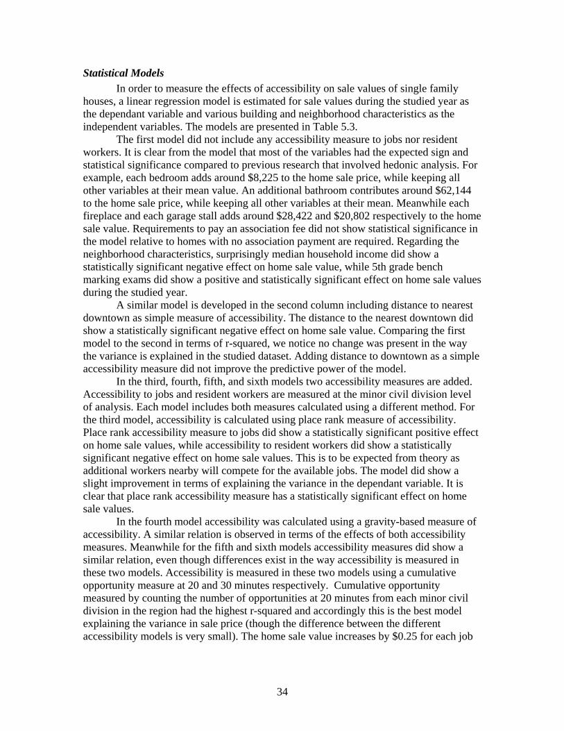
34
Statistical Models In order to measure the effects of accessibility on sale values of single family
houses, a linear regression model is estimated for sale values during the studied year as the dependant variable and various building and neighborhood characteristics as the independent variables. The models are presented in Table 5.3.
The first model did not include any accessibility measure to jobs nor resident workers. It is clear from the model that most of the variables had the expected sign and statistical significance compared to previous research that involved hedonic analysis. For example, each bedroom adds around $8,225 to the home sale price, while keeping all other variables at their mean value. An additional bathroom contributes around $62,144 to the home sale price, while keeping all other variables at their mean. Meanwhile each fireplace and each garage stall adds around $28,422 and $20,802 respectively to the home sale value. Requirements to pay an association fee did not show statistical significance in the model relative to homes with no association payment are required. Regarding the neighborhood characteristics, surprisingly median household income did show a statistically significant negative effect on home sale value, while 5th grade bench marking exams did show a positive and statistically significant effect on home sale values during the studied year.
A similar model is developed in the second column including distance to nearest downtown as simple measure of accessibility. The distance to the nearest downtown did show a statistically significant negative effect on home sale value. Comparing the first model to the second in terms of r-squared, we notice no change was present in the way the variance is explained in the studied dataset. Adding distance to downtown as a simple accessibility measure did not improve the predictive power of the model.
In the third, fourth, fifth, and sixth models two accessibility measures are added. Accessibility to jobs and resident workers are measured at the minor civil division level of analysis. Each model includes both measures calculated using a different method. For the third model, accessibility is calculated using place rank measure of accessibility. Place rank accessibility measure to jobs did show a statistically significant positive effect on home sale values, while accessibility to resident workers did show a statistically significant negative effect on home sale values. This is to be expected from theory as additional workers nearby will compete for the available jobs. The model did show a slight improvement in terms of explaining the variance in the dependant variable. It is clear that place rank accessibility measure has a statistically significant effect on home sale values.
In the fourth model accessibility was calculated using a gravity-based measure of accessibility. A similar relation is observed in terms of the effects of both accessibility measures. Meanwhile for the fifth and sixth models accessibility measures did show a similar relation, even though differences exist in the way accessibility is measured in these two models. Accessibility is measured in these two models using a cumulative opportunity measure at 20 and 30 minutes respectively. Cumulative opportunity measured by counting the number of opportunities at 20 minutes from each minor civil division in the region had the highest r-squared and accordingly this is the best model explaining the variance in sale price (though the difference between the different accessibility models is very small). The home sale value increases by $0.25 for each job

35
within 20 minutes of travel time from the minor civil division that this home is present in, while keeping all the other measures that affect home sales price at their mean value.

36
Table 5.3: Hedonic analysis with accessibility to jobs and resident workers
No Accessibility Measure Distance to Downtown Place Rank Gravity Based Cumulative 20 Cumulative 30 B t B t B t B t B t B t
(Constant) -55698.7 -3.08* -60861.1 -3.35* -98821 -5.12* -105929 -5.76* -54971.7 -3.02* -12518 -0.67 NUMBR 8225.11 11.27* 8256.77 11.32* 8753.47 12.05* 9249.88 12.75* 9421.94 12.99* 8418.78 11.57* NUMBA 62144.96 75.24* 62105.39 75.2* 61988.01 75.4* 61746.78 75.26* 61591.4 75.08* 61364.11 74.32* AGE 553.7 22.06* 538.54 21.22* 492.76 19.52* 445.36 17.46* 438.04 17.16* 513.89 20.23* AFP 87.42 65.48* 87.52 65.56* 86.43 65* 86.32 65.1* 86.1 64.93* 86.98 65.3* NUMFP 28422.15 35.63* 28298.53 35.46* 27416.45 34.48* 27470.49 34.54* 27448.72 34.52* 27657.79 34.61* NUMGA 20802.29 27.21* 21151.76 27.49* 21472.54 28.2* 21520.17 28.16* 21784.77 28.51* 21828.75 28.37* AREA 45.42 2.79** 45.96 2.82* 43.9 2.71** 43.2 2.67** 43.02 2.66** 42.74 2.63** NEWB 33960.9 2.44** 33205.54 2.38** 34010.49 2.45** 35669.38 2.58** 32055.49 2.32** 31296.15 2.25** PROWN -21238.4 -1.55 -21511.1 -1.57 -21478 -1.58 -19178.8 -1.41 -22416.4 -1.65 -24108 -1.76 YASSO -3990.61 -0.29 -4326.67 -0.32 -4772.9 -0.35 -3901.36 -0.29 -8000.17 -0.59 -5883.1 -0.43 MASSO -7431.43 -1.93 -7489.99 -1.95 -7195.78 -1.88 -7615.88 -1.99 -8038.77 -2.11** -6675.99 -1.74 OASSO -61079.1 -19.78* -61839.3 -19.99* -60069.1 -19.55* -57325.7 -18.66* -57179.7 -18.62* -61731.9 -20.02* CRVIW 33769.56 5.56* 34459.68 5.67* 30553.2 5.05* 29189.43 4.84* 29406.17 4.87* 33709.06 5.56* LAVIW 49312.08 11.34* 50233.29 11.53* 48126.12 11.11* 48124.7 11.13* 46157.37 10.67* 47515.1 10.93* POVIW 8786.29 3.59* 8903.6 3.64* 8725.08 3.59* 8364.13 3.45* 8345.67 3.44* 9659 3.96* RVIW 64226.99 5.09* 64991.15 5.16* 65939.71 5.26* 65110.77 5.2* 65984.11 5.27* 68300.32 5.43* PWHIT -88911.6 -4.44* -85132.8 -4.25* -2999.58 -0.15 15445.41 0.76 54061.43 2.62** -3056.82 -0.15 PBACH 40367.28 5.97* 39463.13 5.84* 15294.04 2.23** 14190.45 2.07** 17896.96 2.61** 10209.43 1.45 PMAST 343579.5 25.76* 336721.5 25.05* 338235.6 25.48* 315746.1 23.76* 323999.2 24.41** 376236.1 27.83* INCOM -0.16 -4.57* -0.14 -3.73* -0.04 -1.23 0.02 0.48 0.01 0.29 -0.08 -2.01** 5GRLEV 9.33 3.00* 10.84 3.46* 2.62 0.84 10.87 3.52* 10.52 3.41* 5.98 1.92 SCHGRR -524.59 -9.03* -498.79 -8.53* 350.05 3.67* 63.67 0.99 -371.08 -6.17* -657.14 -10.76* DOPEN 14.81 10.73* 16.00 11.33* 13.97 10.15* 11.71 8.38* 10.96 7.85* 15.35 10.99* DDTWN -0.24 -3.99* PRJ 0.42 21.23* PRRW -0.45 -9.15* GJ 12.71 25.67* GRW -16.93 -21.96* COJ20 0.25 26.24* CORW20 -0.35 -24.4* COJ30 0.19 15.21* CORW30 -0.23 -14.4*
R2 0.576 0.576 0.580 0.582 0.583 0.578 * Indicates Statistical significance at 99% level of confidence ** Indicates Statistical significance at 95% level of confidence

37
For each resident worker in the region competing for these opportunities, the home sale value is expected to decrease by $0.35, while keeping all the other measures that affects home sale price at their mean value.
It is important to note that model specification did not vary much due to change in the way accessibility was measured. This can be used as an indication for the robustness of the dataset being used. It also increases our confidence level in using any of the proposed models
Discussion It can be concluded from this study that measures of accessibility have a
statistically significant effect on home sale prices. The effects here may be understated, as there is a correlation between other attributes of a house and its accessibility. A well-located house is likely to be improved in other aspects (e.g., square footage or bathrooms), while little investment will be made in poorly placed houses.
The results highlight the importance of accessibility and how people value it. Cumulative opportunity measures of accessibility calculated using 20 minutes of travel time did show to have the highest effect on home sale prices in terms of statistical significance and model fitting. Place rank did show a statistically significant effect on home sale prices similar to the other measures. It is important to note that the difference between all the models in terms of explaining the variation in the home sale values (third, fourth, fifth and six) is minor and not large enough to say that a measure is better than the other in terms of explaining home sale prices.
Appendix E includes a similar comparison. Table E.1 shows four hedonic analysis models with accessibility to jobs measured using four different methods (place rank, gravity-based, cumulative opportunity to jobs in 20 minutes of travel time and cumulative opportunity to jobs in 20 minutes of travel time). The first model, with a place rank measure of accessibility, has a higher r-squared and place rank did show the highest level of statistical significance compared to all the other measures of accessibility. The differences between the models are still small and, all show that accessibility has a statistically significant effect on home sale prices.

38
Chapter 6: ACCESSIBILITY OVER TIME
Introduction The power of any accessibility measure is revealed when it is included in a
longitudinal analysis. Comparison of accessibility measures over time can help public agencies to better understand how well the land use and transportation system is performing. For example, if congestion levels increase in a city while levels of accessibility have increased, then this can be used as an indicator for some kind of success in land use planning or market performance. This chapter demonstrates how changes in accessibility can be compared using a statistical analysis method.
Methodology and data sources When comparing accessibility measures over time, it is important to unify the
data sources and the measure of accessibility being used. For example, if comparing accessibility to jobs in 1990 to accessibility to jobs in 2000, obtaining the number of jobs from the same data source is essential, while if using cumulative opportunity measure fixing the time range and methods for calculating travel time is a key. Comparing cumulative opportunity in 2000 to a gravity-based or place rank accessibility measure in 1990 is not possible since the methods are different and accessibility is a relative measure. Vollum (1996) conducted an analysis to measure accessibility using cumulative opportunity in some TAZs in the Twin Cities region for the year 1990. In his study he measures accessibility to jobs and resident workers. For travel time information, he used data obtained form the Metropolitan Council’s transportation planning model during the morning peak in the studied year, while his source for population and number of resident workers was the US Census Bureau. Accessibility to jobs was calculated from 10 different TAZs in the region, while accessibility to workers was measured from 11 TAZs. Similarly we obtained travel time for the year 2000 from the Metropolitan Council’s transportation planning model and we obtained the same datasets from the US Census Bureau to conduct a comparative analysis of accessibility over time. Figure 6.1 shows the location of the TAZs that were selected by Vollum (1996) in his study. The cumulative opportunity measure was calculated at the 30, 45 and 60 minutes of travel time from each TAZ of origin for the 1990 time period. Similarly the same cumulative opportunity measures are calculated for the year 2000.

39
Figure 6.1: Selected TAZ for the comparative study
Detailed Comparative Study As is clear from Figure 6.1 the selected TAZs for the study are dispersed and the
sample is small (21 observations). Table 6.1 includes a summary of the cumulative opportunity measures of accessibility to jobs obtained from the Vollum (1996) presentation for the 1990 accessibility measured at these TAZs. Also accessibility is reported for the year 2000 measured using cumulative opportunity measures.
Table 6.1: Comparative analysis of cumulative opportunity to jobs
Cumulative Opportunity 1990 Cumulative Opportunity 2000 ID TAZ location 30 MIN 45 MIN 60 MIN 30MIN 45 MIN 60 MIN
63 NE Coon Rapids 590707 1184024 1268827 644335 1342616 1501995 139 NE Chanhassen 496776 1148186 1272445 565316 1306132 1492699 185 N Central Lakeville 502256 1184105 1278982 764536 1424366 1521253 373 Inner Minneapolis 1193011 1276471 1284215 1395120 1511870 1524205 501 N Central Bloomington 1109762 1272442 1283279 1257434 1509065 1523788 787 Central Maple Grove 658448 1195604 1274110 712232 1367898 1510357 840 Inner St. Paul 880959 1244795 1277576 957349 1473606 1514070 904 Macal St Paul 1130503 1272028 1282828 1287642 1502583 1522568 1053 NE Prior Lake 350887 1121307 1274634 452335 1319684 1512416 1103 E Central Woodbury 519676 1195946 1277215 518034 1372227 1510527
Data Sources Travel time: Met Council Selection: Mn/DOT GIS Files: US Census 2000

40
Table 6.2 includes a similar comparison for cumulative opportunity measure of
accessibility to residents.
Table 6.2: Comparative analysis of cumulative opportunity to residents Cumulative Opportunity 1990 Cumulative Opportunity 2000 ID TAZ location
30 MIN 45 MIN 60 MIN 30 MIN 45 MIN 60 MIN 85 Central Blaine 1309933 2009244 2241642 1284782 2184400 2583347
193 Burnsville Center 1213623 2055632 2264258 1311269 2394264 2612135 253 N. Central Eagan 1486646 2109030 2267759 1667212 2435844 2624283 308 International Airport 1557260 2148446 2279622 1845676 2508435 2634707 408 Minneapolis CBD 1870534 2214011 2284438 2207639 2575465 2640733 544 N E Eden Prairie 1331867 2115518 2271675 1635577 2497141 2629229 663 S. Cent Plymouth 1366657 2107737 2281347 1614105 2460591 2633423 816 St. Paul CBD 1674497 2186098 2274899 1925616 2544038 2630996 921 3M Campus 1263286 2102113 2260955 1256016 2398189 2602698 931 Maplewood Mall 1452227 2144750 2257790 1522939 2418850 2600732 965 N. of Rosedale 1798235 2203596 2271005 2019628 2556743 2626900
Observing Tables 6.1 and 6.2, it is clear that the number of jobs and residents that
can be reached within 30, 45, and 60 minutes of travel time have increased in almost all of the studied TAZs. In order to confirm this observation statistically, a difference in means t-test is conducted. The results of the difference in means test are presented in Table 6.3 with the critical value for the t-statistics at the 95% level of confidence. Table 6.3: Difference in means test Cumulative Opportunity to jobs Cumulative Opportunity to residents 30 Min 45 Min 60 Min 30 Min 45 Min 60 Min Mid Point 139,739 292,954 351,715 225,703 468,155 524,716 t Stat 4.456 18.690 118.612 4.701 18.371 180.762
All variables in Table 6.3 did show a statistically significant increase in the
accessibility measures at the 95% confidence level. The number of jobs within 30 minutes of travel time measured from each of the studied TAZs experienced an average increase of 139,739 jobs between 990 and 2000, while the number of jobs within 45 minutes of travel time increased on average by 292,954 jobs. Similarly the number of jobs within 60 minutes did increase on average by 351,715 jobs. Meanwhile the number of residents increased at a higher rate than the number of jobs. The number of residents within 30 minutes of the studied TAZs showed an average increase of 225,703 residents between the years of 1990 and 2000, while the number of residents within 45 minutes of the studied TAZs increased by an average of 468,155 residents and the average number of residents residing within 60 minutes of travel time from the studied TAZs increased by 524,716 residents.
The increase in the level of accessibility at the studied TAZs indicates a success in the land use and transportation systems that these TAZs experienced. Generalization from this analysis is limited due to the size of the sample, yet it can be used as an indication and help in providing a methodology for comparing accessibility over time. Comparing
41
these findings with levels of delays in the region between the years of 1990 and 2000 can help in better understanding the value of the accessibility measure. In 1990 the average annual delay per person during the peak period was 19 hours, while in 2000 the average annual delay per person during the peak period was 43 hours (Schrank & Lomax, 2005). This indicates an increase in the level of congestion that each traveler is exposed to during the morning peak in the Twin Cities region rose by more than the 100% during the period between 1990 and 2000.
Using this morning congestion measure solely would lead us to conclude that there was a failure in how the transportation system is performing in the region. Yet the urban transportation system is too complex for one measure to evaluate its success or failure. In addition, the transportation system cannot be separated from the land use and economic forces in the region, which drive the development, yet governments and planning authorities can have an effect on accessibility if they are viable economically. Accordingly accessibility measures can be used as a better indicator for the performance of the land use and transportation system in a region, since it incorporates both travel times and changes in density, type, and location of activities (changes in opportunities).
General Comparative Study
In this section a general comparison is conducted between levels of accessibility, using cumulative opportunity measures, in two time periods (1990 and 2000) using two modes of transportation (Auto and Transit). This comparison is conducted measuring accessibility to the number of jobs in each TAZ within 15 minutes of travel time. Travel time for auto and transit are obtained from the Metropolitan Council transportation planning model. For auto, travel time is determined based on morning commute using shortest network path. Transit travel time accounts for both in-vehicle and out-of-vehicle travel time, which includes time associated walking from TAZ centroids to the nearest bus stop, waiting time at the stop derived from the schedules, in-vehicle travel time obtained from schedules, and egress time from the nearest bus stop to the centroid of the destination TAZ. The transit travel time calculations account for a maximum of two transfers and waiting time associated to them. It also accounts for the possibility of driving to park and ride locations between TAZs if service was not available near the centroids.
Figure 6.2 shows the level of cumulative opportunity measure of accessibility to the number of jobs that can be reached within 15 minutes of travel time from each TAZ during the morning peak in year 1990 using auto, while Figure 6.3 shows a similar measure for the year 2000. Similarly Figure 6.4 shows the number of jobs that can be reached within 15 minutes of travel time from each TAZ during the morning peak in the year 1990 using transit and Figure 6.5 shows that information for the year 2000.

42
Figure 6.2: Number of jobs within 15 minutes of travel time in the year 1990 (Auto)
Figure 6.3: Number of jobs within 15 minutes of travel time in the year 2000 (Auto)
Data Sources Travel time: Met Council Selection: Mn/DOT GIS Files: US Census 2000
Data Sources Travel time: Met Council Selection: Mn/DOT GIS Files: US Census 2000

43
Figure 6.4: Number of jobs within 15 minutes of travel time in the year 1990 (Transit)
Figure 6.5: Number of jobs within 15 minutes of travel time in the year 2000 (Transit)
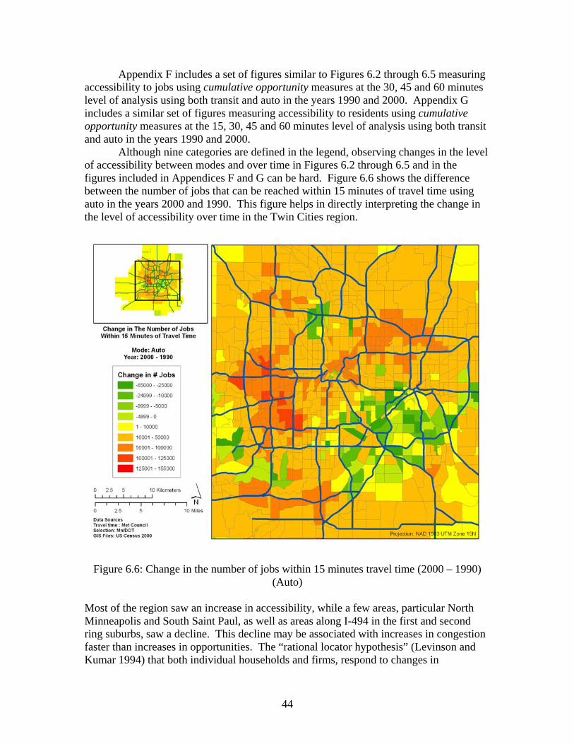
44
Appendix F includes a set of figures similar to Figures 6.2 through 6.5 measuring accessibility to jobs using cumulative opportunity measures at the 30, 45 and 60 minutes level of analysis using both transit and auto in the years 1990 and 2000. Appendix G includes a similar set of figures measuring accessibility to residents using cumulative opportunity measures at the 15, 30, 45 and 60 minutes level of analysis using both transit and auto in the years 1990 and 2000.
Although nine categories are defined in the legend, observing changes in the level of accessibility between modes and over time in Figures 6.2 through 6.5 and in the figures included in Appendices F and G can be hard. Figure 6.6 shows the difference between the number of jobs that can be reached within 15 minutes of travel time using auto in the years 2000 and 1990. This figure helps in directly interpreting the change in the level of accessibility over time in the Twin Cities region.
Figure 6.6: Change in the number of jobs within 15 minutes travel time (2000 – 1990) (Auto)
Most of the region saw an increase in accessibility, while a few areas, particular North Minneapolis and South Saint Paul, as well as areas along I-494 in the first and second ring suburbs, saw a decline. This decline may be associated with increases in congestion faster than increases in opportunities. The “rational locator hypothesis” (Levinson and Kumar 1994) that both individual households and firms, respond to changes in

45
transportation supply by locating themselves to reduce commuting times may be an important explanatory factor in the increase in accessibility. As congestion worsens, firms continue to suburbanize to be near their labor force, and retailers suburbanize to be near their customers, thereby increasing accessibility in suburban areas. Individual homeowners reorient themselves as well, choosing commutes that maximize their personal benefit, including travel time and home attributes.
Similarly Figure 6.7 shows the difference between the number of jobs that can be reached within 15 minutes of travel time during the morning peak using transit as the mode of transportation in the year 2000 and 1990.
Figure 6.7: Change in the number of jobs within 15 minutes travel time (2000 – 1990)
(Transit) It is clear from Figure 6.7 that changes in the number of jobs that can be reached
within 15 minutes of travel time during the morning peak using transit is minor between the years 1990 and 2000, when compared to the change that was observed in Figure 6.6 for auto. This is in part due to the lower accessibility available by transit than by auto. A decline was present in the level of accessibility in most areas however, the only increases were found in the downtown areas and a few random zones.
This may be due to the increase in the number of bus routes and frequency of service in this part of the region. Meanwhile downtown Saint Paul did observe an increase in the level of accessibility to jobs at a lower rate compared to downtown Minneapolis.

46
Figure 6.8: Change in the number of people within 15 minutes travel time (2000 – 1990)
(Auto)

47
Figure 6.9: Change in the number of people within 15 minutes travel time (2000 – 1990)
(Transit)
Figures 6.8 and 6.9 show similar results for number of people within 15 minutes travel time by auto and transit respectively.
Changes in Accessibility to Special Destinations Observing the network structure of the Twin Cities, it is clear that this region is a well connected one. During uncongested time periods, a person can drive from the far East side of the region to the far West in less than 25 minutes. (The width of the region on is around 40 km (24 miles) traveled at an average speed of 96 km/hr (60 miles/hour.) The Twin Cities is a region in which most of the desired activities can be reached within 20 minutes of travel. Accordingly we will use this number to measure accessibility to people from the some of the major attractions in the region. In each city there are major attractions to people residing in it, in these art of the analysis we have chosen seven different attractions. Figures 6.10 and 6.11, and Table 6.4, show the change in the number of people that can be reached within 20 minutes of travel during the morning peak between the years 1990 and 2000 using auto and transit, respectively.
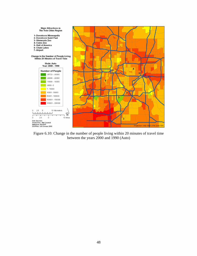
48
Figure 6.10: Change in the number of people living within 20 minutes of travel time
between the years 2000 and 1990 (Auto)

49
Figure 6.11: Change in the number of people living within 20 minutes of travel time
between the years 2000 and 1990 (Transit) Table 6.4: Change in the number of people within 20 minutes of special destinations between the years 2000 and 1990 Auto Transit 1990 2000 % of Change 1990 2000 % of Change 1- Downtown Minneapolis 1181834 1221413 3.24% 43989 48472 9.25% 2- Downtown Saint Paul 937288 981343 4.49% 10808 41669 74.06% 3- Minnesota Zoo 404621 443993 8.87% 14214 19326 26.45% 4- Como Zoo 844245 872369 3.22% 28456 12111 -134.96% 5- Mall of America 938084 978660 4.15% 2114 4622 54.26% 6- Chain Lakes 793595 811443 2.20% 55718 17456 -219.19% 7- Airport 833771 898892 7.24% 4095 894 -358.05%
50
Chapter 7: CONCLUSIONS
Introduction This report introduced the importance of accessibility as a measure of land use
and transportation performance. Also it introduced the importance of such measures to both individuals and public agencies. The report synthesized the literature on accessibility performance measures, and described the available data for the Twin Cities region, to develop a set of accessibility measures that can be used to trace historical trends in a way that is meaningful across time. These measures were illustrated using both hypothetical and real data sets to demonstrate how each measure behaves and differs from the others.
Measures of Accessibility The goal of this research was to develop a set of possible performance
measurements that can be used to analyze variable sets of historic land use and travel time data, including data from the freeway networks and surface streets, transit systems, and non-motorized travel to understand accessibility. These measures can be used in a variety of operational planning and public involvement activities of transportation agencies to ascertain how investments, transportation strategies, and land use policies affect the performance of the transportation-land use system.
Several accessibility measures were reviewed and demonstrated in this report. Cumulative opportunity and gravity-based measures tend to be similar when travel time is less than or equal to 30 minutes. The gravity-based measure is widely used in the literature yet cumulative opportunity tends to be easier to understand. It was clear that similarities exist in all of the studied measures of accessibility. Similarities were observed using both visual and statistical methods. Several measures of accessibility were conducted for Twin Cities region using estimated travel time obtained from Metropolitan Council’s transportation planning model. The availability of a comprehensive dataset including work and resident information at the census block level analysis allowed the testing of a new accessibility measure: “place rank.”
Place Rank Place rank is a new accessibility measure that accounts for the number of
opportunities that an individual foregoes in a zone to reach an opportunity in another zone. Since origins and destination of actual choices are known (jobs and residence), the impedance function that is used in traditional gravity-based accessibility measures is embedded in the origin and destination matrix. Place rank shares some similarities with other commonly used measures of accessibility. Place rank appears to be a promising measure of accessibility, but more work is needed to determine the appropriate unit of analysis that can be used to generate such measure. The major disadvantage of this measure is in terms of the complexity of calculations and the diminishing effect that zones with low levels of attractiveness are observing. The major advantage is that travel time is not needed and accordingly no estimations are incorporated in the analysis. The data used in place rank can be obtained from the U.S. Census Bureau.
51
Applications Several accessibility measures were tested and selected based on the literature
review conducted during the first task and feedback from the technical advisory panel. Accessibility to jobs was used as the main example to compare the various measures, while accessibility to resident workers, and retail and non-retail jobs were also demonstrated using gravity-based, cumulative opportunity, and place rank measures. Each accessibility measure was tested and illustrated to demonstrate the workability and typical results of the proposed methods. Real land use data (number of jobs and number of resident workers) was coupled with modeled travel time data for a single point in time (AM peak for the Year 2000). The use of observed travel time data was not yet possible since such data is not readily available in a usable form. Use of actual data is anticipated to be performed as part of a subsequent project.
Measurement Errors It is important to note that the travel time used in this report was obtained from a
transportation planning model, and not from directly measured transportation data. The use of such model can impose a measurement error to the analysis. For instance, relatively small inconsistencies in the model application or errors in the calibration between 1990 and 2000 may change a small decrease in accessibility to a small increase. Yet it remains the best available estimate for travel time in the Twin Cities region. Other projects being conducted as part of the Access to Destinations aim to estimate travel time using various modes of transportation from either archived traffic data along freeways and arterials and/or transit schedules, and will help in better estimating the travel time and decrease the potential error associated with using estimates from transportation planning models.
Effects of Accessibility It was clear from chapter five that accessibility measures do have an effect on
home sale values. Place rank measure of accessibility did show a similar effect as all the other measures of accessibility on home sale values. Accessibility to jobs did show a statistically significant and positive effect on home sale value, while resident workers do show a statistically significant negative effect on home sale value too.
The value of accessibility to individuals is reflected in the home sale price, which highlights how it affects willingness to pay relative to location.
Time Series The importance of accessibility as a measure of land use and transportation
planning performance in a region was explored by comparing it over time. The longitudinal analysis being conducted did show improvements along the studied TAZs in terms of the level of accessibility. The findings were compared tentatively to the levels of congestion in the region between the same time periods. This comparison did show the difference between the two measures and strengthened the importance of accessibility measures as a tool for monitoring and evaluating land use and transportation planning performance in a region.

52
Future Research After the completion of various ongoing and proposed projects at the University
of Minnesota, travel time based on archived data and improved estimates will be available for various points in time. Accordingly, generation of various and more accurate accessibility maps similar to what was demonstrated in this report will be possible. Place Rank did show to be a promising measure of accessibility, yet more research is needed to measure the accuracy and applicability of such measure in other regions and over different geographical aggregations, since it requires origins and destinations information, which is available presently only for journey to work trips.

53
REFERENCES Alexander, C., Ishikawa, S., Silverstein, M., Jacobson, M., Fiksdahl-king, I., & Angel, S.
(1977). A pattern language: Bowns buildings constructions. UK: Oxford University Press.
American Planning Association. (2005). The language of traffic. Retrieved December, 6, 2005, from http://www.planning.org/thecommissioner/19952003/spring02.htm
Baradaran, S., & Ramjerdi, F. (2001). Performance of accessibility measures in Europe. Journal of Transportation Statistics, 4(2/3), 31-48.
Ben-Akiva, M., & Lermand, S. (1977). Disaggregate travel and mobility choice models and measures of accessibility. Paper presented at the Proceedings of the Third International Conference on Behavioral Travel Modeling, Tanenda, Australia.
Brin, S., & Page, L. (1998). The Anatomy of a Large-Scale Hypertextual Web Search Engine. Computer Networks, 30(1-7), 107-117.
Filipi, M. (2005). Travel time for the Twin Cities region. In A. El-Geneidy & D. Levinson (Eds.). Minneapolis, MN.
Franklin, J., & Waddell. (2003). A hedonic regression of home prices in King County, Washington using activity-specific accessibility measures. Paper presented at the Transportation Research Board 82nd Annual Meeting, Washington DC.
Giuliano, G. (2004). Land use impacts of transportation investments: Highway and transit. In S. Hanson & G. Genevieve (Eds.), The Geography of Urban Transportation (Third ed.). New York: The Guilford Press.
Handy, S. L. (1994). Highway blues: Nothing a little accessibility can't cure. Access, 5, 3-7.
Handy, S. L. (2002). Accessibility -vs mobility- enhancing strategies for addressing automobile dependence in the US. Paper presented at the European Conference of Ministers of Transport, Tokyo, Japan.
Handy, S. L., & Niemeier, D. A. (1997). Measuring accessibility: An exploration of issues and alternatives. Environment and Planning A, 29(7), 1175-1194.
Hansen, W. (1959). How accessibility shape land use. Journal of the American Institute of Planners, 25(2), 73-76.
Koenig, J. G. (1980). Indicators of urban accessibility: Theory and application. Transportation, 9, 145-172.
LEHD. (2003). Longitudinal employer household dynamics (No. ID-2003-03). Suitland, MD: US Census Bureau, LEHD Program.
Levinson, D., & Krizek, K. (2005). The machine for access. In D. Levinson & K. Krizek (Eds.), Access to Destinations (pp. 1-10). Netherlands: Elsevier Inc.
Levinson, D. and Kumar. A. (1994) The Rational Locator: Why Travel Times Have Remained Stable. Journal of the American Planning Association, Summer 1994 60:3 319-332.
Miller, H. (1999). GIS software for measuring space-time accessibility in transportation planning analysis. Paper presented at the International Workshop on Geographic Information Systems for Transportation and Intelligent Transportation Systems, Hong Kong.

54
Miller, H. (2005). Place-based versus people-based accessibility. In D. Levinson & K. Krizek (Eds.), Access to Destinations (pp. 63-89). Netherlands: Elsevier Inc.
Miller, H., & Shaw, S. (2001). Geographic information systems for transportation: Principles and applications. New York: Oxford University Press.
Minnesota Department of Transportation. (2003). Strategic Plan 2003. Retrieved February 13, 2005, from http://www.dot.state.mn.us/information/statplan00/index.html#vision
Murray, A., & Wu, X. (2003). Accessibility tradeoffs in public transit planning. Journal of Geographical Systems, 5(1), 93-107.
Neuburger, H. (1971). User benefits in the evaluation of transport and land use plans. Journal of Transportation Economics and Policy, 5, 52-75.
Schrank, D., & Lomax, T. (2005). The 2005 urban mobility report: Texas Transportation Institute.
Sirmans, S., & Macpherson, D. (2003). The composition of hedonic pricing models: A review of the literature. Chicago, IL: National Association of Relators.
Srour, I., Kockelman, K., & Dunn, T. (2002). Accessibility indices: Connection to residential land prices and location choices. Transportation Research Record(1805), 25-34.
Talen, E. (1998). Visualizing fairness: Equity maps for planners. Journal of the American Planning Association, 64(1), 22-38.
U.S. Census Bureau. (2000, January, 2005). American fact finder. from http://factfinder.census.gov/home/saff/main.html
United States Department of Transportation. (1966). Mission and History. Retrieved February 13, 2005, from http://www.dot.gov/mission.htm
Vickerman, R. W. (1974). Accessibility, attraction and potential: A review of some concepts and their use in determining mobility. Environment and Planning A, 6, 675-691.
Vollum, B. (1996). Highway accessibility maps and data: Suggested findings/conclusions. Minneapolis, MN: Minnesota Department of Transportation.
Wachs, M., & Kumagai, T. (1973). Physical accessibility as a social indicator. Socioeconomic Planning Science, 7, 327-456.
Wu, Y.-H., & Miller, H. (2002). Computational tools for measuring space-time accessibility within transportation networks with dynamic flow," (special issue on accessibility). Journal of Transportation and Statistics, 4(2/3), 1-14.

APPENDIX A: CUMULATIVE OPPORTUNITY MEASURE AT TAZ LEVEL MEASURING ACCESS TO JOBS

A-1
Figure A.1: Number of jobs within 15 minutes of travel time during the morning peak
Data Sources Travel time: Met Council Transportation Model Employment Data: CURA, University of Minnesota GIS Files: US Census 2000

A-2
Figure A.2: Number of jobs within 20 minutes of travel time during the morning peak
Data Sources Travel time: Met Council Transportation Model Employment Data: CURA, University of Minnesota GIS Files: US Census 2000

A-3
Figure A.3: Number of jobs within 25 minutes of travel time during the morning peak
Data Sources Travel time: Met Council Transportation Model Employment Data: CURA, University of Minnesota GIS Files: US Census 2000

A-4
Figure A.4: Number of jobs within 30 minutes of travel time during the morning peak
Data Sources Travel time: Met Council Transportation Model Employment Data: CURA, University of Minnesota GIS Files: US Census 2000

A-5
Figure A.5: Number of jobs within 35 minutes of travel time during the morning peak
Data Sources Travel time: Met Council Transportation Model Employment Data: CURA, University of Minnesota GIS Files: US Census 2000

A-6
Figure A.6: Number of jobs within 40 minutes of travel time during the morning peak
Data Sources Travel time: Met Council Transportation Model Employment Data: CURA, University of Minnesota GIS Files: US Census 2000
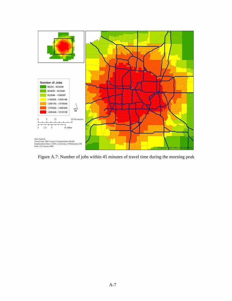
A-7
Figure A.7: Number of jobs within 45 minutes of travel time during the morning peak
Data Sources Travel time: Met Council Transportation Model Employment Data: CURA, University of Minnesota GIS Files: US Census 2000

A-8
Figure A.8: Number of jobs within 50 minutes of travel time during the morning peak
Data Sources Travel time: Met Council Transportation Model Employment Data: CURA, University of Minnesota GIS Files: US Census 2000
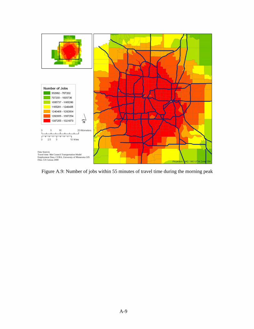
A-9
Figure A.9: Number of jobs within 55 minutes of travel time during the morning peak
Data Sources Travel time: Met Council Transportation Model Employment Data: CURA, University of Minnesota GIS Files: US Census 2000
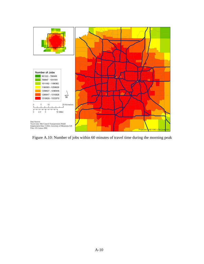
A-10
Figure A.10: Number of jobs within 60 minutes of travel time during the morning peak
Data Sources Travel time: Met Council Transportation Model Employment Data: CURA, University of Minnesota GIS Files: US Census 2000

APPENDIX B: CUMULATIVE OPPORTUNITY MEASURE AT TAZ LEVEL MEASURING ACCESS TO WORKERS

B-1
Figure B.1: Number of resident workers within 10 minutes of travel time during the morning peak
Data Sources Travel time: Met Council Transportation Model Employment Data: CURA, University of Minnesota GIS Files: US Census 2000
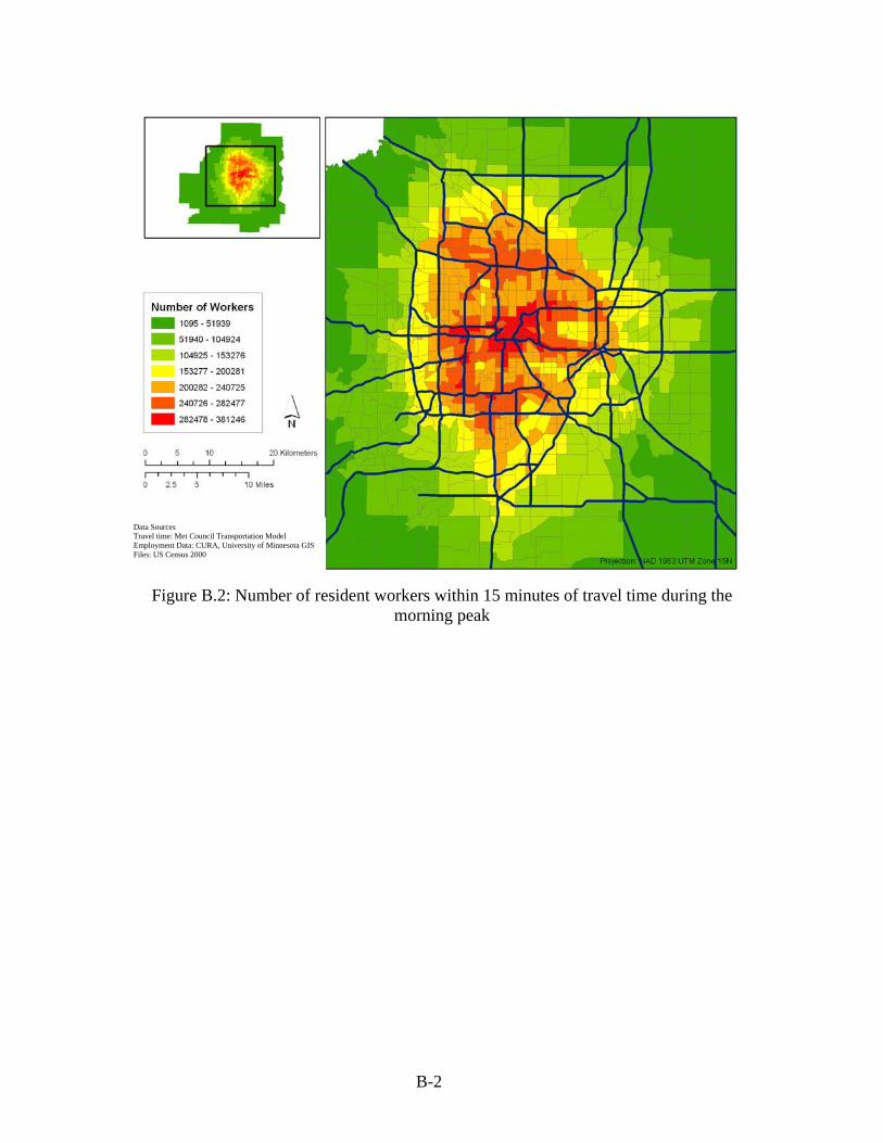
B-2
Figure B.2: Number of resident workers within 15 minutes of travel time during the
morning peak
Data Sources Travel time: Met Council Transportation Model Employment Data: CURA, University of Minnesota GIS Files: US Census 2000

APPENDIX C: CUMULATIVE OPPORTUNITY MEASURE AT TAZ LEVEL MEASURING ACCESS TO RETAIL AND NON-RETAIL JOBS

C-1
Figure C.1: Number of retail jobs within 10 minutes of travel time during the morning peak

C-2
Figure C.2: Number of non-retail jobs within 10 minutes of travel time during the morning peak
Data Sources Travel time: Met Council Transportation Model Employment Data: CURA, University of Minnesota GIS Files: US Census 2000

C-3
Figure C.3: Number of retail jobs within 15 minutes of travel time during the morning peak
Data Sources Travel time: Met Council Transportation Model Employment Data: CURA, University of Minnesota GIS Files: US Census 2000
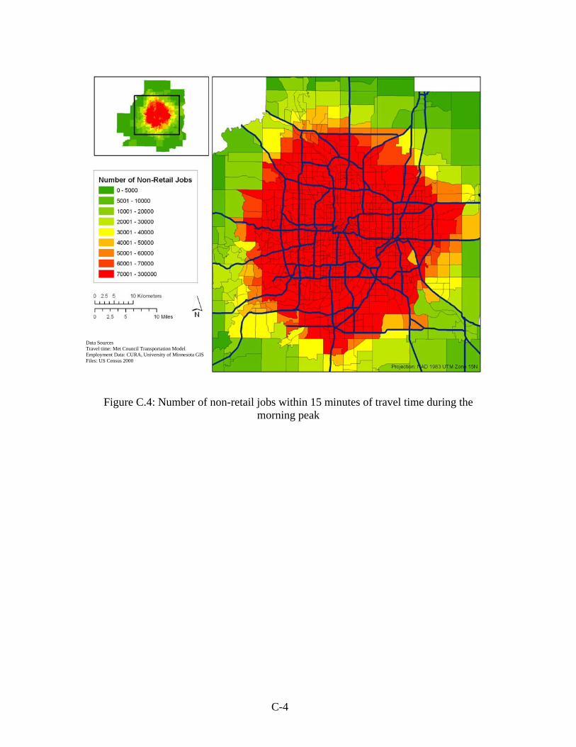
C-4
Figure C.4: Number of non-retail jobs within 15 minutes of travel time during the morning peak
Data Sources Travel time: Met Council Transportation Model Employment Data: CURA, University of Minnesota GIS Files: US Census 2000

APPENDIX D: ACCESSIBILITY TO RESIDENT WORKERS AT THE MINOR CIVIL DIVISION LEVEL

D-1
Figure D.1: Place rank measuring accessibility to resident workers
Data Sources Employment Data: CURA, University of Minnesota GIS Files: US Census 2000
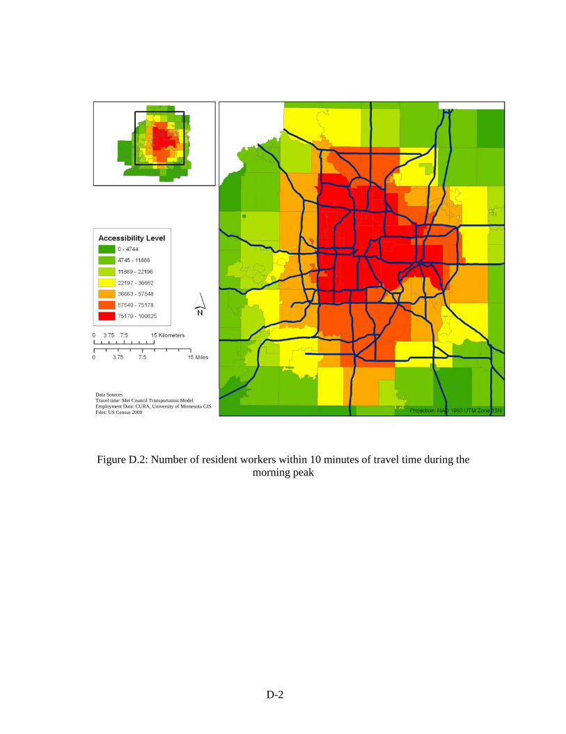
D-2
Figure D.2: Number of resident workers within 10 minutes of travel time during the morning peak
Data Sources Travel time: Met Council Transportation Model Employment Data: CURA, University of Minnesota GIS Files: US Census 2000
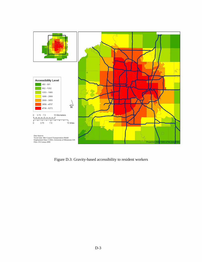
D-3
Figure D.3: Gravity-based accessibility to resident workers
Data Sources Travel time: Met Council Transportation Model Employment Data: CURA, University of Minnesota GIS Files: US Census 2000

APPENDIX E: ACCESSIBILITY TO RESIDENT WORKERS AT THE MINOR CIVIL DIVISION LEVEL

E-1
Table E.1: Hedonic analysis with accessibility to jobs
Place Rank Gravity Based Cumulative 20 Cumulative 30 B t B t B t B t
(Constant) -145458.92 -7.81* -109024.20 -5.89* -83731.22 -4.57* -70843.90 -3.88* NUMBR 8535.08 11.74* 8507.90 11.68* 8427.29 11.56* 8278.26 11.35* NUMBA 61839.85 75.17* 62327.35 75.60* 62292.68 75.48* 62165.06 75.29*
AGE 484.19 19.17* 483.94 18.92* 507.32 19.87* 528.54 20.78* AFP 86.93 65.37* 87.27 65.49* 87.33 65.47* 87.46 65.53*
NUMFP 27715.70 34.85* 27414.93 34.29* 27690.32 34.59* 27986.77 34.95* NUMGA 21477.05 28.18* 21998.56 28.64* 21690.07 28.20* 21390.20 27.76* AREA 44.49 2.74** 45.85 2.82* 45.78 2.81* 45.67 2.81** NEWB 32967.64 2.38** 34022.41 2.45** 33662.19 2.42** 33753.74 2.42**
PROWN -22048.54 -1.62 -21001.32 -1.54 -21411.67 -1.56 -21571.21 -1.57 YASSO -4376.53 -0.32 -4858.74 -0.36 -5033.22 -0.37 -4427.64 -0.32 MASSO -6965.34 -1.82 -7102.48 -1.85 -7193.80 -1.87 -7249.14 -1.89 OASSO -59955.95 -19.49* -61604.11 -19.99* -61711.82 -20.00* -61923.21 -20.04* CRVIW 31932.88 5.28* 33863.19 5.58* 33771.71 5.56* 34235.22 5.63* LAVIW 49609.44 11.45* 51790.34 11.92* 51043.96 11.74* 50507.82 11.60* POVIW 8844.85 3.63* 9507.34 3.90* 9240.42 3.78* 9103.64 3.72* RVIW 67673.57 5.39* 66649.77 5.30* 66110.16 5.25* 65828.10 5.22*
PWHIT -2246.73 -0.11 -60269.24 -3.00* -66195.29 -3.29* -76122.34 -3.78* PBACH 15383.20 2.25** 21000.14 3.05* 26916.81 3.91* 31426.27 4.54* PMAST 336531.24 25.33* 329976.76 24.72* 334984.64 25.09* 341475.64 25.61* INCOM -0.04 -1.17 0.00 -0.05 -0.05 -1.36 -0.10 -2.73**
5GRLEV 4.27 1.37 9.98 3.22* 9.75 3.14* 9.14 2.94* SCHGRR 716.09 8.27* -168.14 -2.64** -357.99 -5.91* -448.41 -7.54* DOPEN 14.80 10.77* 16.86 12.17* 16.31 11.76* 16.18 11.57*
PRJ 0.36 19.28* GJ 3.94 13.40**
COJ20 0.03 9.62* COJ30 0.01 5.95*
R2 0.580 0.578 0.577 0.577 * Indicates Statistical significance at 99% level of confidence ** Indicates Statistical significance at 95% level of confidence

APPENDIX F: CUMULATIVE OPPORTUNITY MEASURE AT TAZ LEVEL MEASURING ACCESS TO JOBS OVER TIME USING AUTO AND TRANSIT
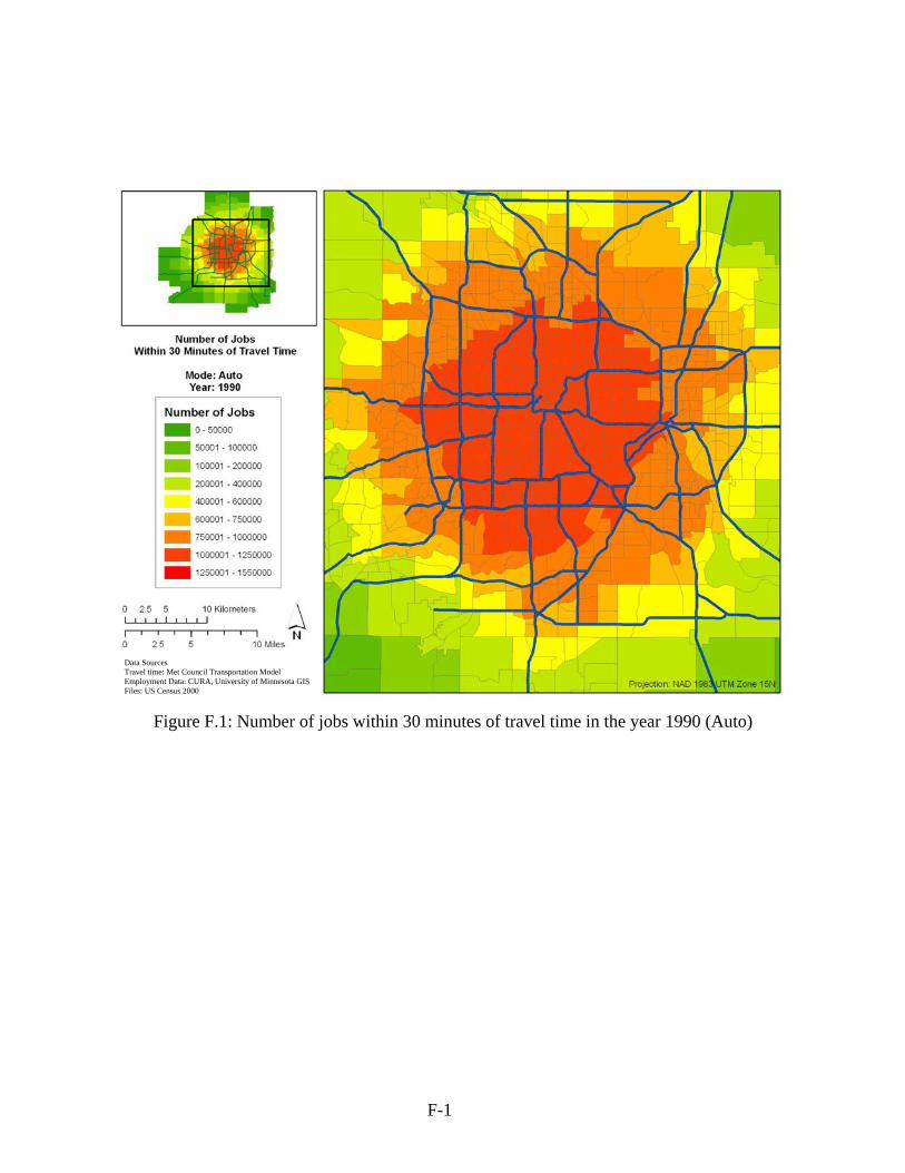
F-1
Figure F.1: Number of jobs within 30 minutes of travel time in the year 1990 (Auto)
Data Sources Travel time: Met Council Transportation Model Employment Data: CURA, University of Minnesota GIS Files: US Census 2000

F-2
Figure F.2: Number of jobs within 30 minutes of travel time in the year 2000 (Auto)
Data Sources Travel time: Met Council Transportation Model Employment Data: CURA, University of Minnesota GIS Files: US Census 2000

F-3
Figure F.3: Number of jobs within 30 minutes of travel time in the year 1990 (Transit)
Data Sources Travel time: Met Council Transportation Model Employment Data: CURA, University of Minnesota GIS Files: US Census 2000

F-4
Figure F.4: Number of jobs within 30 minutes of travel time in the year 2000 (Transit)
Data Sources Travel time: Met Council Transportation Model Employment Data: CURA, University of Minnesota GIS Files: US Census 2000

F-5
Figure F.5: Number of jobs within 45 minutes of travel time in the year 1990 (Auto)
Data Sources Travel time: Met Council Transportation Model Employment Data: CURA, University of Minnesota GIS Files: US Census 2000

F-6
Figure F.6: Number of jobs within 45 minutes of travel time in the year 2000 (Auto)
Data Sources Travel time: Met Council Transportation Model Employment Data: CURA, University of Minnesota GIS Files: US Census 2000

F-7
Figure F.7: Number of jobs within 45 minutes of travel time in the year 1990 (Transit)
Data Sources Travel time: Met Council Transportation Model Employment Data: CURA, University of Minnesota GIS Files: US Census 2000

F-8
Figure F.8: Number of jobs within 45 minutes of travel time in the year 2000 (Transit)
Data Sources Travel time: Met Council Transportation Model Employment Data: CURA, University of Minnesota GIS Files: US Census 2000

F-9
Figure F.9: Number of jobs within 60 minutes of travel time in the year 1990 (Auto)
Data Sources Travel time: Met Council Transportation Model Employment Data: CURA, University of Minnesota GIS Files: US Census 2000

F-10
Figure F.10: Number of jobs within 60 minutes of travel time in the year 2000 (Auto)
Data Sources Travel time: Met Council Transportation Model Employment Data: CURA, University of Minnesota GIS Files: US Census 2000
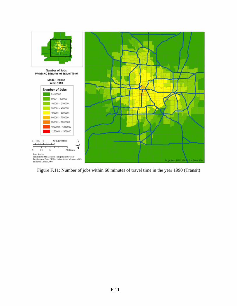
F-11
Figure F.11: Number of jobs within 60 minutes of travel time in the year 1990 (Transit)
Data Sources Travel time: Met Council Transportation Model Employment Data: CURA, University of Minnesota GIS Files: US Census 2000

F-12
Figure F.12: Number of jobs within 60 minutes of travel time in the year 2000 (Transit)
Data Sources Travel time: Met Council Transportation Model Employment Data: CURA, University of Minnesota GIS Files: US Census 2000

APPENDIX G: CUMULATIVE OPPORTUNITY MEASURE AT TAZ LEVEL MEASURING ACCESS TO JOBS OVER TIME USING AUTO AND TRANSIT

G-1
Figure G.1: Number of people living within 15 minutes of travel time in the year 1990 (Auto)
Data Sources Travel time: Met Council Transportation Model Employment Data: CURA, University of Minnesota GIS Files: US Census 2000
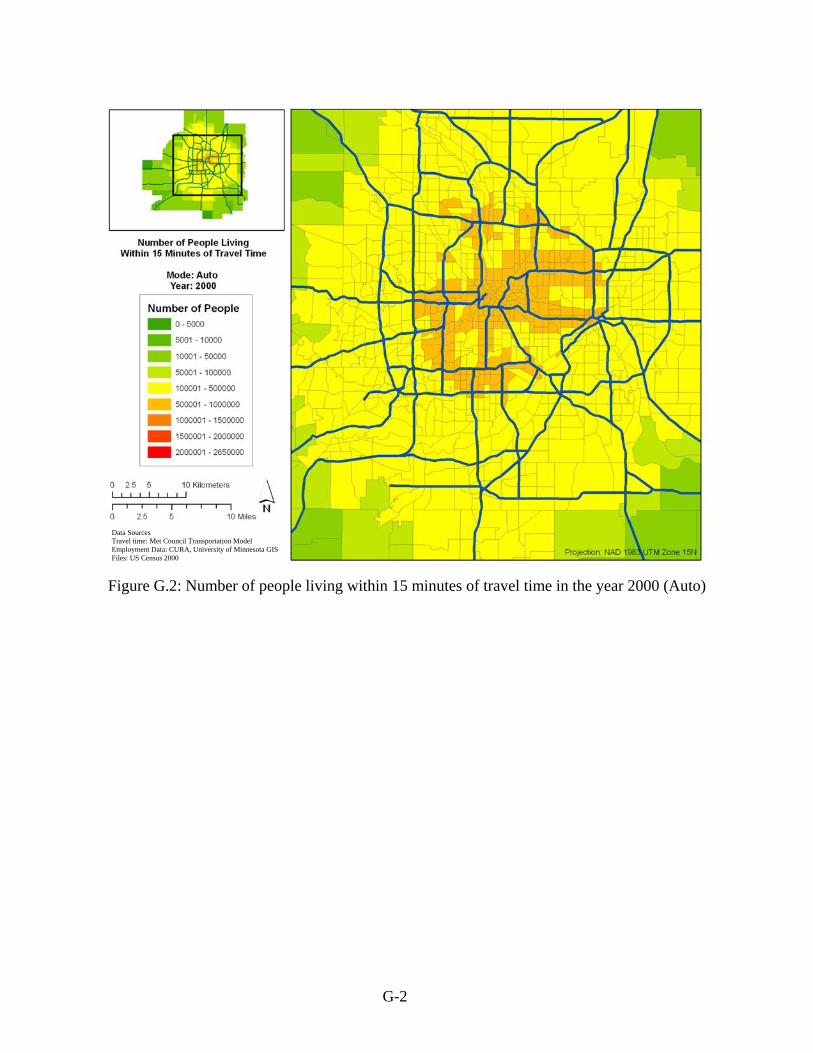
G-2
Figure G.2: Number of people living within 15 minutes of travel time in the year 2000 (Auto)
Data Sources Travel time: Met Council Transportation Model Employment Data: CURA, University of Minnesota GIS Files: US Census 2000

G-3
Figure G.3: Number of people living within 15 minutes of travel time in the year 1990 (Transit)
Data Sources Travel time: Met Council Transportation Model Employment Data: CURA, University of Minnesota GIS Files: US Census 2000

G-4
Figure G.4: Number of people living within 15 minutes of travel time in the year 2000 (Transit)
Data Sources Travel time: Met Council Transportation Model Employment Data: CURA, University of Minnesota GIS Files: US Census 2000
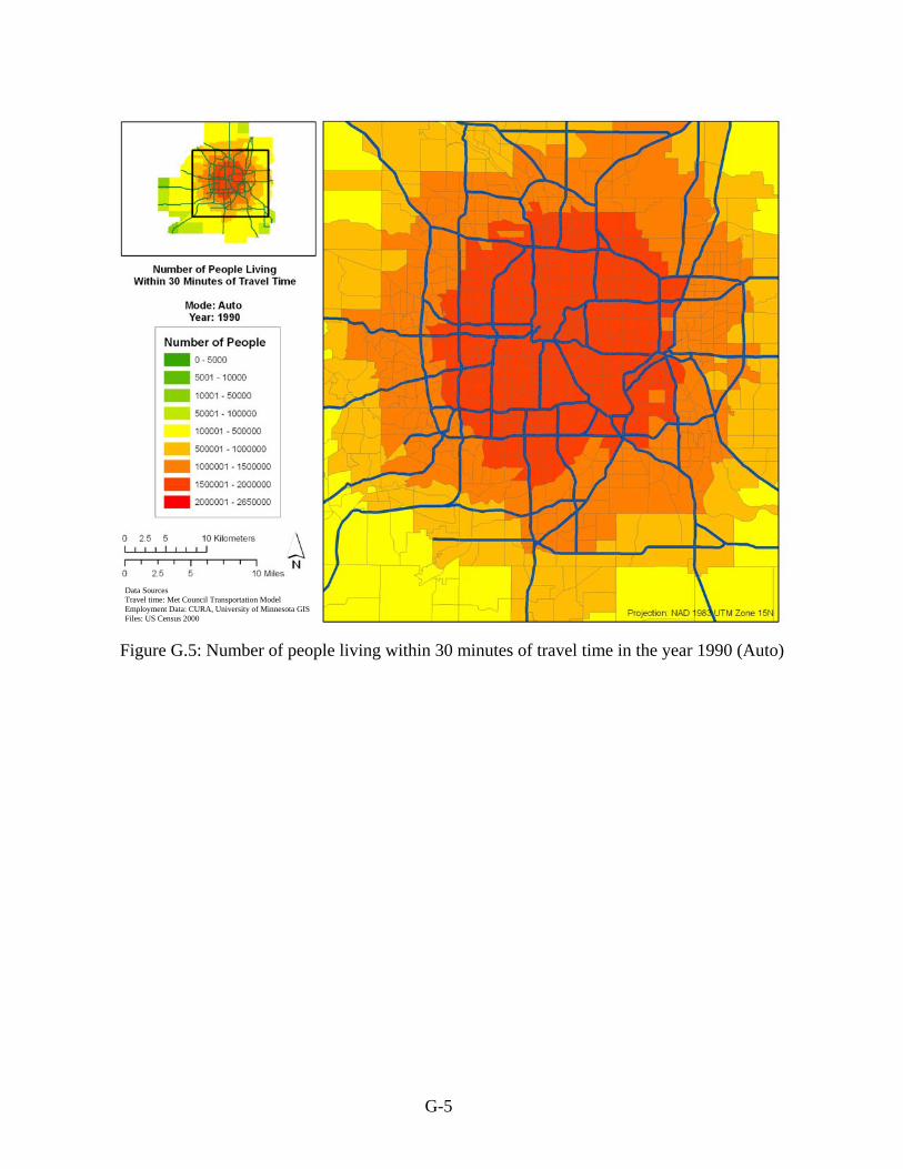
G-5
Figure G.5: Number of people living within 30 minutes of travel time in the year 1990 (Auto)
Data Sources Travel time: Met Council Transportation Model Employment Data: CURA, University of Minnesota GIS Files: US Census 2000

G-6
Figure G.6: Number of people living within 30 minutes of travel time in the year 2000 (Auto)
Data Sources Travel time: Met Council Transportation Model Employment Data: CURA, University of Minnesota GIS Files: US Census 2000
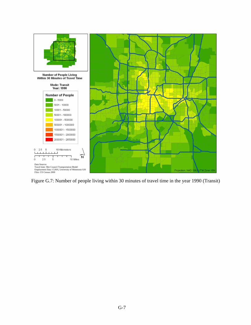
G-7
Figure G.7: Number of people living within 30 minutes of travel time in the year 1990 (Transit)
Data Sources Travel time: Met Council Transportation Model Employment Data: CURA, University of Minnesota GIS Files: US Census 2000

G-8
Figure G.8: Number of people living within 30 minutes of travel time in the year 2000 (Transit)
Data Sources Travel time: Met Council Transportation Model Employment Data: CURA, University of Minnesota GIS Files: US Census 2000

G-9
Figure G.9: Number of people living within 45 minutes of travel time in the year 1990 (Auto)
Data Sources Travel time: Met Council Transportation Model Employment Data: CURA, University of Minnesota GIS Files: US Census 2000

G-10
Figure G.10: Number of people living within 45 minutes of travel time in the year 2000 (Auto)
Data Sources Travel time: Met Council Transportation Model Employment Data: CURA, University of Minnesota GIS Files: US Census 2000
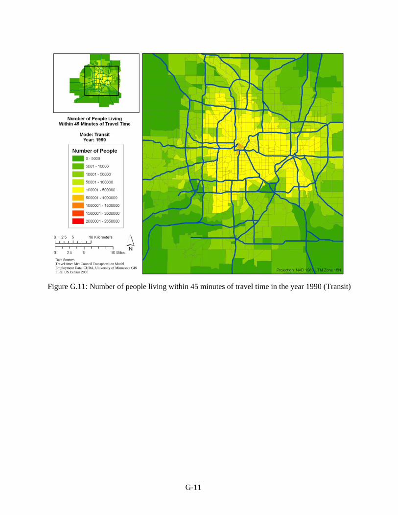
G-11
Figure G.11: Number of people living within 45 minutes of travel time in the year 1990 (Transit)
Data Sources Travel time: Met Council Transportation Model Employment Data: CURA, University of Minnesota GIS Files: US Census 2000

G-12
Figure G.12: Number of people living within 45 minutes of travel time in the year 2000 (Transit)
Data Sources Travel time: Met Council Transportation Model Employment Data: CURA, University of Minnesota GIS Files: US Census 2000

G-13
Figure G.13: Number of people living within 60 minutes of travel time in the year 1990 (Auto)
Data Sources Travel time: Met Council Transportation Model Employment Data: CURA, University of Minnesota GIS Files: US Census 2000
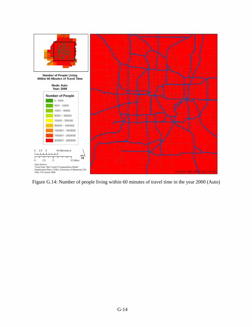
G-14
Figure G.14: Number of people living within 60 minutes of travel time in the year 2000 (Auto)
Data Sources Travel time: Met Council Transportation Model Employment Data: CURA, University of Minnesota GIS Files: US Census 2000

G-15
Figure G.15: Number of people living within 60 minutes of travel time in the year 1990 (Transit)
Data Sources Travel time: Met Council Transportation Model Employment Data: CURA, University of Minnesota GIS Files: US Census 2000

G-16
Figure G.16: Number of people living within 60 minutes of travel time in the year 2000 (Transit)
Data Sources Travel time: Met Council Transportation Model Employment Data: CURA, University of Minnesota GIS Files: US Census 2000