Acceptors as Values

Functional Programming in Classical Linear Logic

(Technical Summary)

Uday S. ReddyDepartment of Computer Science

University of Illinois at Urbana-Champaign

Urbana, IL 61801

Net: reddy@cs.uiuc.edu

December 9, 1991

Abstract

Girard’s linear logic has been previously applied to functional programming for per-forming state-manipulation and controlling storage reuse. These applications only useintuitionistic linear logic, the subset of linear logic that embeds intuitionistic logic. Fulllinear logic (called classical linear logic) is much richer than this subset. In this paper, weconsider the application of classical linear logic to functional programming. The negativetypes of linear logic are interpreted as denoting acceptors. An acceptor is an entity whichtakes an input of some type and returns no output. Acceptors generalize continuations andalso single assignment variables, as found in data flow languages and logic programminglanguages. The parallel disjunction operator allows such acceptors to be used in a nontrivialfashion. Finally, the “why not” operator of linear logic gives rise to nondeterministic values.We define a typed functional language based on the these ideas and demonstrate its use viaexamples. The language has a reduction semantics that generalizes typed lambda calculus,and satisfies strong normalization and Church-Rosser properties.

Keywords Linear logic, propositions-as-types isomorphism, sequent calculus, continua-tions, single assignment variables, logic variables, acceptors, bivalent types, nondetermin-ism, strong normalization, confluence.

1

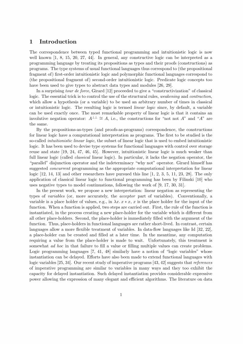
1 Introduction

The correspondence between typed functional programming and intuitionistic logic is nowwell known [1, 8, 15, 20, 27, 44]. In general, any constructive logic can be interpreted as aprogramming language by treating its propositions as types and their proofs (constructions) asprograms. The type systems of usual functional languages thus correspond to (the propositionalfragment of) first-order intuitionistic logic and polymorphic functional languages correspond to(the propositional fragment of) second-order intuitionistic logic. Predicate logic concepts toohave been used to give types to abstract data types and modules [26, 29].

In a surprising tour de force, Girard [12] proceeded to give a “constructivization” of classicallogic. The essential trick is to control the use of the structural rules, weakening and contraction,which allow a hypothesis (or a variable) to be used an arbitrary number of times in classicalor intuitionistic logic. The resulting logic is termed linear logic since, by default, a variablecan be used exactly once. The most remarkable property of linear logic is that it contains aninvolutive negation operator: A⊥⊥ ∼= A, i.e., the constructions for “not not A” and “A” arethe same.

By the propositions-as-types (and proofs-as-programs) correspondence, the constructionsfor linear logic have a computational interpretation as programs. The first to be studied is theso-called intuitionistic linear logic, the subset of linear logic that is used to embed intuitionisticlogic. It has been used to devise type systems for functional languages with control over storagereuse and state [19, 24, 47, 46, 45]. However, intuitionistic linear logic is much weaker thanfull linear logic (called classical linear logic). In particular, it lacks the negation operator, the“parallel” disjunction operator and the indeterminacy “why not” operator. Girard himself hassuggested concurrent programming as the appropriate computational interpretation for linearlogic [12, 14, 13] and other researchers have pursued this line [1, 2, 3, 5, 11, 23, 28]. The onlyapplication of classical linear logic to functional programming has been by Filinski [10] whouses negative types to model continuations, following the work of [9, 17, 30, 31].

In the present work, we propose a new interpretation: linear negation as representing thetypes of variables (or, more accurately, the acceptor part of variables). Conventionally, avariable is a place holder of values, e.g., in λx. x ∗ x, x is the place holder for the input of thefunction. When a function is applied, two steps are carried out. First, the rule of the function isinstantiated, in the process creating a new place-holder for the variable which is different fromall other place-holders. Second, the place-holder is immediately filled with the argument of thefunction. Thus, place-holders in functional languages are rather short-lived. In contrast, certainlanguages allow a more flexible treatment of variables. In data-flow languages like Id [32, 22],a place-holder can be created and filled at a later time. In the meantime, any computationrequiring a value from the place-holder is made to wait. Unfortunately, this treatment issomewhat ad hoc in that failure to fill a value or filling multiple values can create problems.Logic programming languages [7, 41, 48] similarly have a notion of “logic variables” whoseinstantiation can be delayed. Efforts have also been made to extend functional languages withlogic variables [25, 34]. Our recent study of imperative programs [43, 42] suggests that references

of imperative programming are similar to variables in many ways and they too exhibit thecapacity for delayed instantiation. Such delayed instantiation provides considerable expressivepower allowing the expression of many elegant and efficient algorithms. The literature on data

1

flow languages, logic programming and imperative programming contains several examples ofthis expressive power.

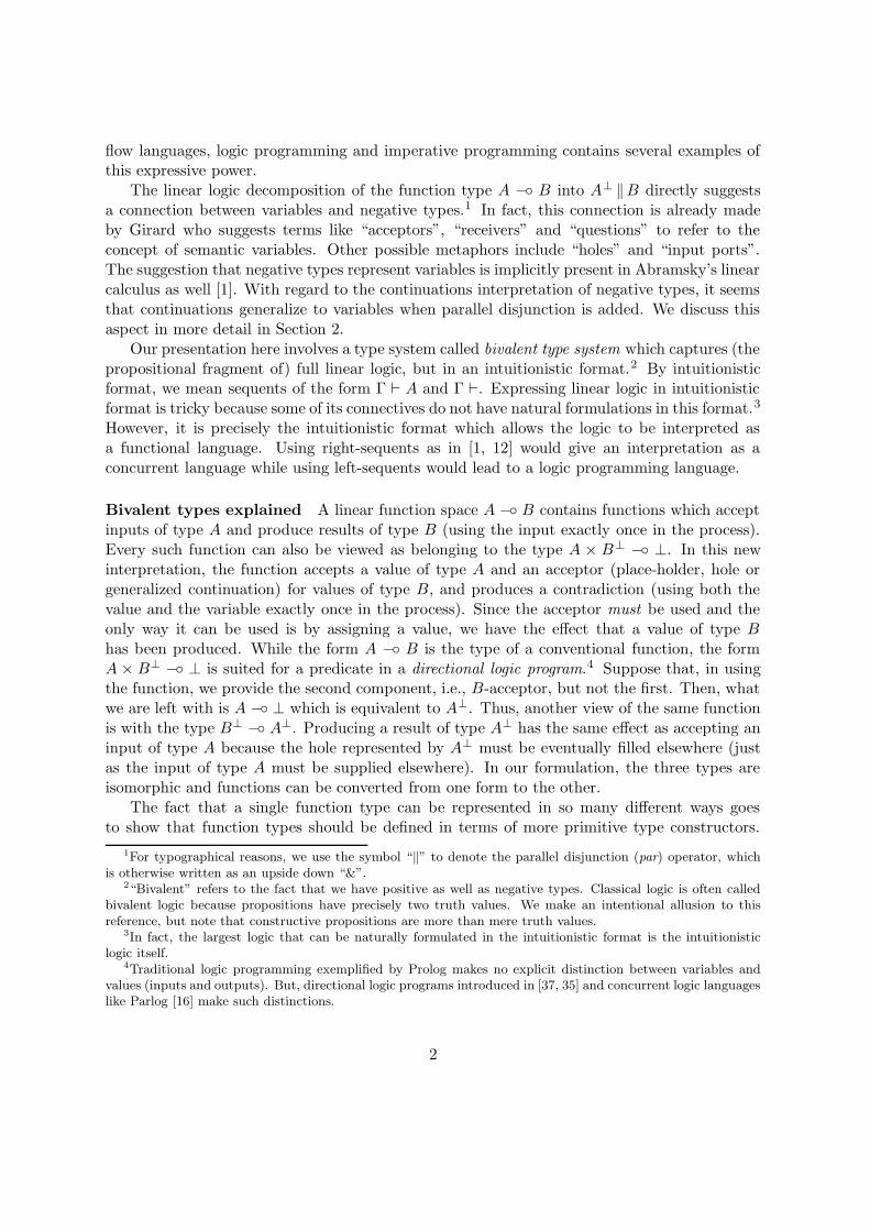
The linear logic decomposition of the function type A −◦ B into A⊥ ‖B directly suggestsa connection between variables and negative types.1 In fact, this connection is already madeby Girard who suggests terms like “acceptors”, “receivers” and “questions” to refer to theconcept of semantic variables. Other possible metaphors include “holes” and “input ports”.The suggestion that negative types represent variables is implicitly present in Abramsky’s linearcalculus as well [1]. With regard to the continuations interpretation of negative types, it seemsthat continuations generalize to variables when parallel disjunction is added. We discuss thisaspect in more detail in Section 2.

Our presentation here involves a type system called bivalent type system which captures (thepropositional fragment of) full linear logic, but in an intuitionistic format.2 By intuitionisticformat, we mean sequents of the form Γ ` A and Γ `. Expressing linear logic in intuitionisticformat is tricky because some of its connectives do not have natural formulations in this format.3

However, it is precisely the intuitionistic format which allows the logic to be interpreted asa functional language. Using right-sequents as in [1, 12] would give an interpretation as aconcurrent language while using left-sequents would lead to a logic programming language.

Bivalent types explained A linear function space A −◦ B contains functions which acceptinputs of type A and produce results of type B (using the input exactly once in the process).Every such function can also be viewed as belonging to the type A × B⊥ −◦ ⊥. In this newinterpretation, the function accepts a value of type A and an acceptor (place-holder, hole orgeneralized continuation) for values of type B, and produces a contradiction (using both thevalue and the variable exactly once in the process). Since the acceptor must be used and theonly way it can be used is by assigning a value, we have the effect that a value of type Bhas been produced. While the form A −◦ B is the type of a conventional function, the formA × B⊥ −◦ ⊥ is suited for a predicate in a directional logic program.4 Suppose that, in usingthe function, we provide the second component, i.e., B-acceptor, but not the first. Then, whatwe are left with is A −◦ ⊥ which is equivalent to A⊥. Thus, another view of the same functionis with the type B⊥ −◦ A⊥. Producing a result of type A⊥ has the same effect as accepting aninput of type A because the hole represented by A⊥ must be eventually filled elsewhere (justas the input of type A must be supplied elsewhere). In our formulation, the three types areisomorphic and functions can be converted from one form to the other.

The fact that a single function type can be represented in so many different ways goesto show that function types should be defined in terms of more primitive type constructors.

1For typographical reasons, we use the symbol “‖” to denote the parallel disjunction (par) operator, whichis otherwise written as an upside down “&”.

2“Bivalent” refers to the fact that we have positive as well as negative types. Classical logic is often calledbivalent logic because propositions have precisely two truth values. We make an intentional allusion to thisreference, but note that constructive propositions are more than mere truth values.

3In fact, the largest logic that can be naturally formulated in the intuitionistic format is the intuitionisticlogic itself.

4Traditional logic programming exemplified by Prolog makes no explicit distinction between variables andvalues (inputs and outputs). But, directional logic programs introduced in [37, 35] and concurrent logic languageslike Parlog [16] make such distinctions.

2

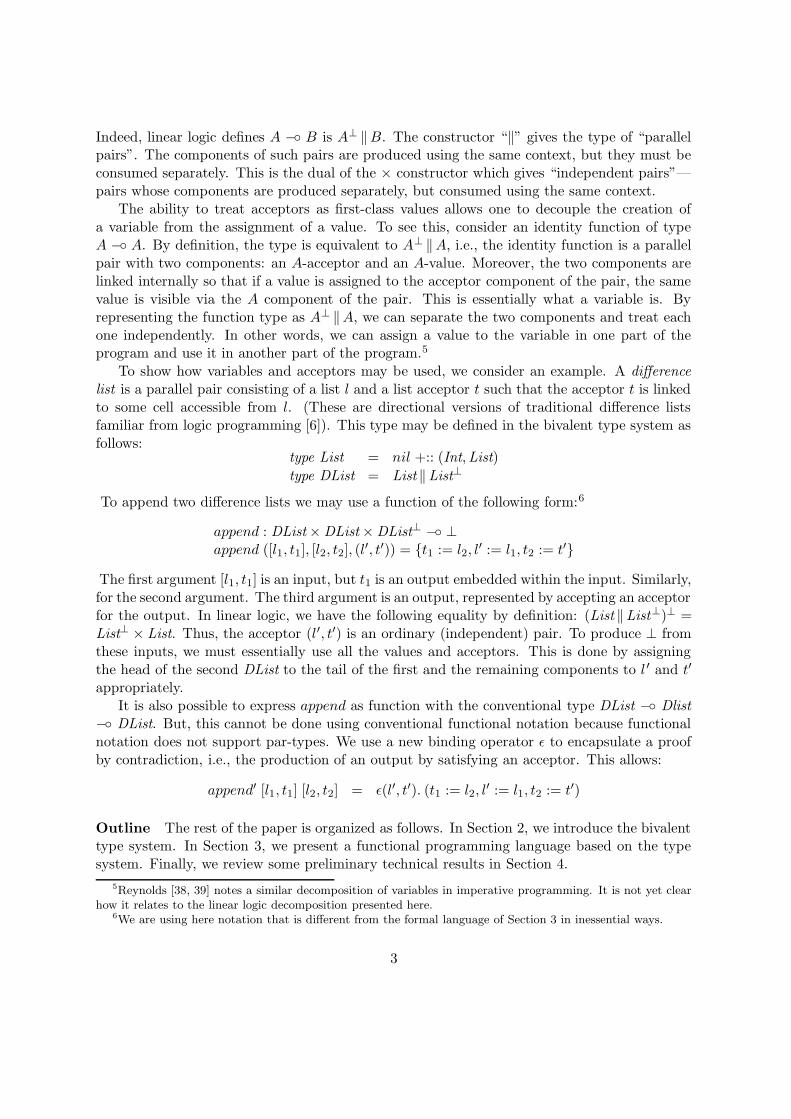
Indeed, linear logic defines A −◦ B is A⊥ ‖B. The constructor “‖” gives the type of “parallelpairs”. The components of such pairs are produced using the same context, but they must beconsumed separately. This is the dual of the × constructor which gives “independent pairs”—pairs whose components are produced separately, but consumed using the same context.

The ability to treat acceptors as first-class values allows one to decouple the creation ofa variable from the assignment of a value. To see this, consider an identity function of typeA −◦ A. By definition, the type is equivalent to A⊥ ‖A, i.e., the identity function is a parallelpair with two components: an A-acceptor and an A-value. Moreover, the two components arelinked internally so that if a value is assigned to the acceptor component of the pair, the samevalue is visible via the A component of the pair. This is essentially what a variable is. Byrepresenting the function type as A⊥ ‖A, we can separate the two components and treat eachone independently. In other words, we can assign a value to the variable in one part of theprogram and use it in another part of the program.5

To show how variables and acceptors may be used, we consider an example. A difference

list is a parallel pair consisting of a list l and a list acceptor t such that the acceptor t is linkedto some cell accessible from l. (These are directional versions of traditional difference listsfamiliar from logic programming [6]). This type may be defined in the bivalent type system asfollows:

type List = nil +:: (Int,List)

type DList = List ‖List⊥

To append two difference lists we may use a function of the following form:6

append : DList × DList × DList⊥ −◦ ⊥append ([l1, t1], [l2, t2], (l

′, t′)) = {t1 := l2, l′ := l1, t2 := t′}

The first argument [l1, t1] is an input, but t1 is an output embedded within the input. Similarly,for the second argument. The third argument is an output, represented by accepting an acceptorfor the output. In linear logic, we have the following equality by definition: (List ‖List⊥)⊥ =List⊥ × List. Thus, the acceptor (l′, t′) is an ordinary (independent) pair. To produce ⊥ fromthese inputs, we must essentially use all the values and acceptors. This is done by assigningthe head of the second DList to the tail of the first and the remaining components to l ′ and t′

appropriately.It is also possible to express append as function with the conventional type DList −◦ Dlist

−◦ DList. But, this cannot be done using conventional functional notation because functionalnotation does not support par-types. We use a new binding operator ε to encapsulate a proofby contradiction, i.e., the production of an output by satisfying an acceptor. This allows:

append′ [l1, t1] [l2, t2] = ε(l′, t′). (t1 := l2, l′ := l1, t2 := t′)

Outline The rest of the paper is organized as follows. In Section 2, we introduce the bivalenttype system. In Section 3, we present a functional programming language based on the typesystem. Finally, we review some preliminary technical results in Section 4.

5Reynolds [38, 39] notes a similar decomposition of variables in imperative programming. It is not yet clearhow it relates to the linear logic decomposition presented here.

6We are using here notation that is different from the formal language of Section 3 in inessential ways.

3

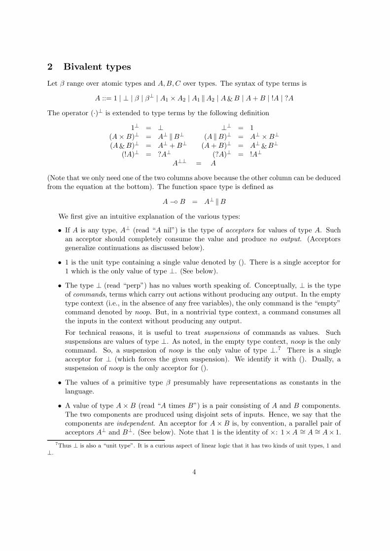
2 Bivalent types

Let β range over atomic types and A,B,C over types. The syntax of type terms is

A ::= 1 | ⊥ | β | β⊥ | A1 ×A2 | A1 ‖A2 | A&B | A+B | !A | ?A

The operator (·)⊥ is extended to type terms by the following definition

1⊥ = ⊥ ⊥⊥ = 1(A×B)⊥ = A⊥ ‖B⊥ (A ‖B)⊥ = A⊥ ×B⊥

(A&B)⊥ = A⊥ +B⊥ (A+B)⊥ = A⊥ &B⊥

(!A)⊥ = ?A⊥ (?A)⊥ = !A⊥

A⊥⊥ = A

(Note that we only need one of the two columns above because the other column can be deducedfrom the equation at the bottom). The function space type is defined as

A −◦ B = A⊥ ‖B

We first give an intuitive explanation of the various types:

• If A is any type, A⊥ (read “A nil”) is the type of acceptors for values of type A. Suchan acceptor should completely consume the value and produce no output. (Acceptorsgeneralize continuations as discussed below).

• 1 is the unit type containing a single value denoted by (). There is a single acceptor for1 which is the only value of type ⊥. (See below).

• The type ⊥ (read “perp”) has no values worth speaking of. Conceptually, ⊥ is the typeof commands, terms which carry out actions without producing any output. In the emptytype context (i.e., in the absence of any free variables), the only command is the “empty”command denoted by noop. But, in a nontrivial type context, a command consumes allthe inputs in the context without producing any output.

For technical reasons, it is useful to treat suspensions of commands as values. Suchsuspensions are values of type ⊥. As noted, in the empty type context, noop is the onlycommand. So, a suspension of noop is the only value of type ⊥.7 There is a singleacceptor for ⊥ (which forces the given suspension). We identify it with (). Dually, asuspension of noop is the only acceptor for ().

• The values of a primitive type β presumably have representations as constants in thelanguage.

• A value of type A× B (read “A times B”) is a pair consisting of A and B components.The two components are produced using disjoint sets of inputs. Hence, we say that thecomponents are independent. An acceptor for A×B is, by convention, a parallel pair ofacceptors A⊥ and B⊥. (See below). Note that 1 is the identity of ×: 1×A ∼= A ∼= A× 1.

7Thus ⊥ is also a “unit type”. It is a curious aspect of linear logic that it has two kinds of unit types, 1 and⊥.

4

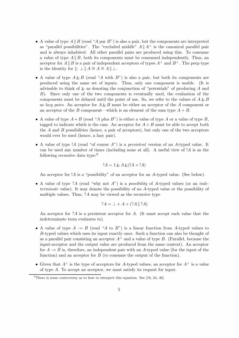
• A value of type A ‖B (read “A par B”) is also a pair, but the components are interpretedas “parallel possibilities”. The “excluded middle” A ‖A⊥ is the canonical parallel pairand is always inhabited. All other parallel pairs are produced using this. To consumea value of type A ‖B, both its components must be consumed independently. Thus, anacceptor for A ‖B is a pair of independent acceptors of types A⊥ and B⊥. The perp typeis the identity for ‖: ⊥‖A ∼= A ∼= A ‖⊥.

• A value of type A&B (read “A with B”) is also a pair, but both its components areproduced using the same set of inputs. Thus, only one component is usable. (It isadvisable to think of & as denoting the conjunction of “potentials” of producing A andB). Since only one of the two components is eventually used, the evaluation of thecomponents must be delayed until the point of use. So, we refer to the values of A&Bas lazy pairs. An acceptor for A&B must be either an acceptor of the A component oran acceptor of the B component—which is an element of the sum type A+B.

• A value of type A+B (read “A plus B”) is either a value of type A or a value of type B,tagged to indicate which is the case. An acceptor for A+B must be able to accept boththe A and B possibilities (hence, a pair of acceptors), but only one of the two acceptorswould ever be used (hence, a lazy pair).

• A value of type !A (read “of course A”) is a persistent version of an A-typed value. Itcan be used any number of times (including none at all). A useful view of !A is as thefollowing recursive data type:8

!A = 1 &A&(!A× !A)

An acceptor for !A is a “possibility” of an acceptor for an A-typed value. (See below).

• A value of type ?A (read “why not A”) is a possibility of A-typed values (or an inde-

terminate value). It may denote the possibility of no A-typed value or the possibility ofmultiple values. Thus, ?A may be viewed as the recursive type

?A = ⊥ +A+ (?A ‖ ?A)

An acceptor for ?A is a persistent acceptor for A. (It must accept each value that theindeterminate term evaluates to).

• A value of type A −◦ B (read “A to B”) is a linear function from A-typed values toB-typed values which uses its input exactly once. Such a function can also be thought ofas a parallel pair consisting an acceptor A⊥ and a value of type B. (Parallel, because theinput-acceptor and the output value are produced from the same context). An acceptorfor A −◦ B is, therefore, an independent pair with an A-typed value (for the input of thefunction) and an acceptor for B (to consume the output of the function).

• Given that A⊥ is the type of acceptors for A-typed values, an acceptor for A⊥ is a valueof type A. To accept an acceptor, we must satisfy its request for input.

8There is some controversy as to how to interpret this equation. See [10, 24, 40].

5

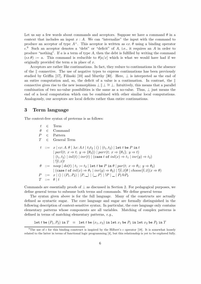
Let us say a few words about commands and acceptors. Suppose we have a command θ in acontext that includes an input x : A. We can “internalize” the input with the command toproduce an acceptor of type A⊥. This acceptor is written as εx. θ using a binding operatorε.9 Such an acceptor denotes a “debt” or “deficit” of A, i.e., it requires an A in order toproduce “nothing”. If a is a term of type A, then the debt is fulfilled by writing the command(εx.θ) := a. This command is reducible to θ[a/x] which is what we would have had if weoriginally provided the term a in place of x.

Acceptors are rather like continuations. In fact, they reduce to continuations in the absenceof the ‖ connective. The use of negative types to express continuations has been previouslystudied by Griffin [17], Filinski [10] and Murthy [30]. Here, ⊥ is interpreted as the end ofan entire computation and, so, the deficit of a value is a continuation. In contrast, the ‖connective gives rise to the new isomorphism ⊥‖⊥ ∼= ⊥. Intuitively, this means that a parallelcombination of two no-value possibilities is the same as a no-value. Thus, ⊥ just means theend of a local computation which can be combined with other similar local computations.Analogously, our acceptors are local deficits rather than entire continuations.

3 Term language

The context-free syntax of preterms is as follows:

t ∈ Termθ ∈ CommandP ∈ PatternT ∈ General Term

t ::= x | εx:A. θ | λx:A.t | t1t2 | () | (t1, t2) | let t be P in t| parl(t; x⇒ t; y ⇒ {θ2}) | parr(t; x⇒ {θ1}; y ⇒ t)| 〈t1, t2〉 | inl(t) | inr(t) | (case t of inl(x) ⇒ t1 | inr(y) ⇒ t2)| ![t; x]t

θ ::= noop | do(t) | t1 := t2 | let t be P in θ | par(t; x⇒ θ1; y ⇒ θ2)| (case t of inl(x) ⇒ θ1 | inr(y) ⇒ θ2) | ![t; x]θ | choose[t; x](x⇒ θ)

P ::= x | () | (P1, P2) | 〈P, 〉 | 〈 , P 〉 | !P | | P1@P2

T ::= θ | t

Commands are essentially proofs of ⊥ as discussed in Section 2. For pedagogical purposes, wedefine general terms to subsume both terms and commands. We define general terms

The syntax given above is for the full language. Many of the constructs are actuallydefined as syntactic sugar. The core language and sugar are formally distinguished in thefollowing description of context-sensitive syntax. In particular, the core language only containselementary patterns whose components are all variables. Matching of complex patterns isdefined in terms of matching elementary patterns, e.g.,

let t be (P1, P2) in T ≡ let t be (x1, x2) in let x1 be P1 in let x2 be P2 in T

9The use of ε for this binding construct is inspired by the Hilbert’s ε operator [18]. It is somewhat looselyrelated to the latter in terms of functional logic programming [4], but this relationship is yet to be explored fully.

6

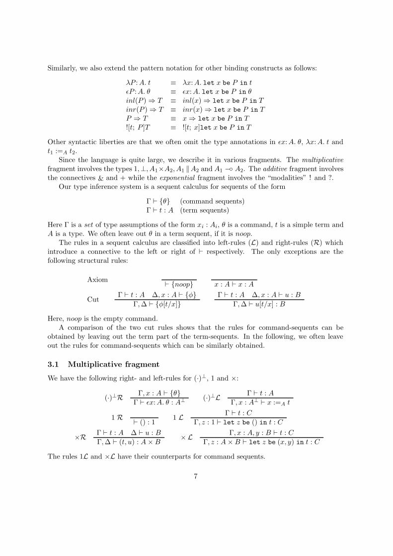
Similarly, we also extend the pattern notation for other binding constructs as follows:

λP :A. t ≡ λx:A. let x be P in tεP :A. θ ≡ εx:A. let x be P in θinl(P ) ⇒ T ≡ inl(x) ⇒ let x be P in Tinr(P ) ⇒ T ≡ inr(x) ⇒ let x be P in TP ⇒ T ≡ x⇒ let x be P in T![t; P ]T ≡ ![t; x]let x be P in T

Other syntactic liberties are that we often omit the type annotations in εx:A. θ, λx:A. t andt1 :=A t2.

Since the language is quite large, we describe it in various fragments. The multiplicative

fragment involves the types 1,⊥, A1×A2, A1 ‖A2 and A1 −◦ A2. The additive fragment involvesthe connectives & and + while the exponential fragment involves the “modalities” ! and ?.

Our type inference system is a sequent calculus for sequents of the form

Γ ` {θ} (command sequents)Γ ` t : A (term sequents)

Here Γ is a set of type assumptions of the form xi : Ai, θ is a command, t is a simple term andA is a type. We often leave out θ in a term sequent, if it is noop.

The rules in a sequent calculus are classified into left-rules (L) and right-rules (R) whichintroduce a connective to the left or right of ` respectively. The only exceptions are thefollowing structural rules:

Axiom` {noop} x : A ` x : A

CutΓ ` t : A ∆, x : A ` {φ}

Γ,∆ ` {φ[t/x]}

Γ ` t : A ∆, x : A ` u : B

Γ,∆ ` u[t/x] : B

Here, noop is the empty command.A comparison of the two cut rules shows that the rules for command-sequents can be

obtained by leaving out the term part of the term-sequents. In the following, we often leaveout the rules for command-sequents which can be similarly obtained.

3.1 Multiplicative fragment

We have the following right- and left-rules for (·)⊥, 1 and ×:

(·)⊥RΓ, x : A ` {θ}

Γ ` εx:A. θ : A⊥(·)⊥L

Γ ` t : A

Γ, x : A⊥ ` x :=A t

1 R` () : 1

1 LΓ ` t : C

Γ, z : 1 ` let z be () in t : C

×RΓ ` t : A ∆ ` u : B

Γ,∆ ` (t, u) : A×B×L

Γ, x : A, y : B ` t : C

Γ, z : A×B ` let z be (x, y) in t : C

The rules 1L and ×L have their counterparts for command sequents.

7

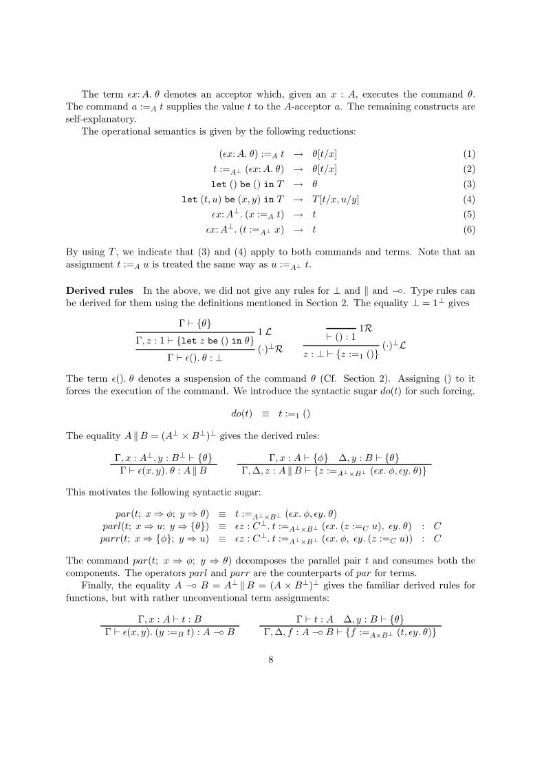
The term εx:A. θ denotes an acceptor which, given an x : A, executes the command θ.The command a :=A t supplies the value t to the A-acceptor a. The remaining constructs areself-explanatory.

The operational semantics is given by the following reductions:

(εx:A. θ) :=A t → θ[t/x] (1)

t :=A⊥ (εx:A. θ) → θ[t/x] (2)

let () be () in T → θ (3)

let (t, u) be (x, y) in T → T [t/x, u/y] (4)

εx:A⊥. (x :=A t) → t (5)

εx:A⊥. (t :=A⊥ x) → t (6)

By using T , we indicate that (3) and (4) apply to both commands and terms. Note that anassignment t :=A u is treated the same way as u :=A⊥ t.

Derived rules In the above, we did not give any rules for ⊥ and ‖ and −◦. Type rules canbe derived for them using the definitions mentioned in Section 2. The equality ⊥ = 1⊥ gives

Γ ` {θ}1 L

Γ, z : 1 ` {let z be () in θ}(·)⊥R

Γ ` ε(). θ : ⊥

1R` () : 1

(·)⊥Lz : ⊥ ` {z :=1 ()}

The term ε(). θ denotes a suspension of the command θ (Cf. Section 2). Assigning () to itforces the execution of the command. We introduce the syntactic sugar do(t) for such forcing.

do(t) ≡ t :=1 ()

The equality A ‖B = (A⊥ ×B⊥)⊥ gives the derived rules:

Γ, x : A⊥, y : B⊥ ` {θ}Γ ` ε(x, y). θ : A ‖B

Γ, x : A ` {φ} ∆, y : B ` {θ}Γ,∆, z : A ‖B ` {z :=A⊥×B⊥ (εx. φ, εy. θ)}

This motivates the following syntactic sugar:

par(t; x⇒ φ; y ⇒ θ) ≡ t :=A⊥×B⊥ (εx. φ, εy. θ)parl(t; x⇒ u; y ⇒ {θ}) ≡ εz : C⊥. t :=A⊥×B⊥ (εx. (z :=C u), εy. θ) : Cparr(t; x⇒ {φ}; y ⇒ u) ≡ εz : C⊥. t :=A⊥×B⊥ (εx. φ, εy. (z :=C u)) : C

The command par(t; x ⇒ φ; y ⇒ θ) decomposes the parallel pair t and consumes both thecomponents. The operators parl and parr are the counterparts of par for terms.

Finally, the equality A −◦ B = A⊥ ‖B = (A × B⊥)⊥ gives the familiar derived rules forfunctions, but with rather unconventional term assignments:

Γ, x : A ` t : B

Γ ` ε(x, y). (y :=B t) : A −◦ BΓ ` t : A ∆, y : B ` {θ}

Γ,∆, f : A −◦ B ` {f :=A×B⊥ (t, εy. θ)}

8

These rules motivate the following syntactic sugar:

λx:A. t ≡ ε(x, y):A×B⊥. (y :=B t) : A −◦ Bt1 t2 ≡ εy:B⊥. {t1 :=A×B⊥ (t2, y)} : B

A function λx:A. t is equivalent to an acceptor which accepts, in addition to the A-typed valuex, a B-acceptor y and supplies the output t to y. Applying such a function involves providingan A-typed input and a B-acceptor.

Note that these reductions imply the following derived reductions for the sugared constructs:

do(ε(). θ) → θpar(ε(x′, y′):A⊥ ×B⊥. ψ; x⇒ φ; y ⇒ θ) → ψ[εx:A. φ/x′, εy:B. θ/y′]

parl(ε(x′, y′):A⊥ ×B⊥. ψ; x⇒ t; y ⇒ {θ}) → t[(εx′:A⊥. ψ[εy:B. θ/y′])/x]parr(ε(x′, y′):A⊥ ×B⊥. ψ; x⇒ {φ}; y ⇒ t) → t[(εy′:B⊥. ψ[εx:A. φ/x′])/y]

(λx:A. t)u → t[u/x]

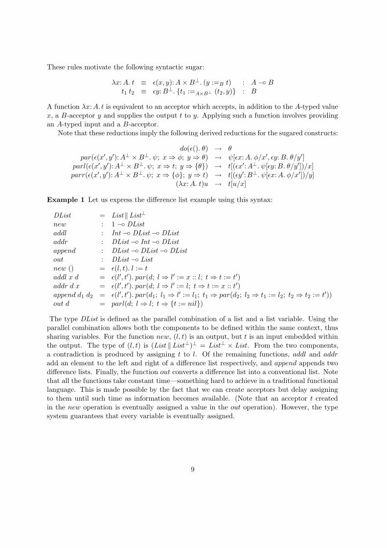
Example 1 Let us express the difference list example using this syntax:

DList = List ‖List⊥

new : 1 −◦ DList

addl : Int −◦ DList −◦ DList

addr : DList −◦ Int −◦ DList

append : DList −◦ DList −◦ DList

out : DList −◦ List

new () = ε(l, t). l := taddl x d = ε(l′, t′). par(d; l ⇒ l′ := x :: l; t⇒ t := t′)addr d x = ε(l′, t′). par(d; l ⇒ l′ := l; t⇒ t := x :: t′)append d1 d2 = ε(l′, t′). par(d1; l1 ⇒ l′ := l1; t1 ⇒ par(d2; l2 ⇒ t1 := l2; t2 ⇒ t2 := t′))out d = parl(d; l ⇒ l; t⇒ {t := nil})

The type DList is defined as the parallel combination of a list and a list variable. Using theparallel combination allows both the components to be defined within the same context, thussharing variables. For the function new, (l, t) is an output, but t is an input embedded withinthe output. The type of (l, t) is (List ‖List⊥)⊥ = List⊥ × List . From the two components,a contradiction is produced by assigning t to l. Of the remaining functions, addl and addradd an element to the left and right of a difference list respectively, and append appends twodifference lists. Finally, the function out converts a difference list into a conventional list. Notethat all the functions take constant time—something hard to achieve in a traditional functionallanguage. This is made possible by the fact that we can create acceptors but delay assigningto them until such time as information becomes available. (Note that an acceptor t createdin the new operation is eventually assigned a value in the out operation). However, the typesystem guarantees that every variable is eventually assigned.

9

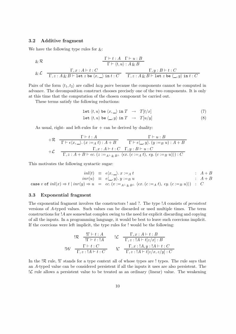
3.2 Additive fragment

We have the following type rules for &:

&RΓ ` t : A Γ ` u : B

Γ ` 〈t, u〉 : A&B

&LΓ, x : A ` t : C

Γ, z : A&B ` let z be 〈x, 〉 in t : C

Γ, y : B ` t : C

Γ, z : A&B ` let z be 〈 , y〉 in t : C

Pairs of the form 〈t1, t2〉 are called lazy pairs because the components cannot be computed inadvance. The decomposition construct chooses precisely one of the two components. It is onlyat this time that the computation of the chosen component be carried out.

These terms satisfy the following reductions:

let 〈t, u〉 be 〈x, 〉 in T → T [t/x] (7)

let 〈t, u〉 be 〈 , y〉 in T → T [u/y] (8)

As usual, right- and left-rules for + can be derived by duality:

+RΓ ` t : A

Γ ` ε〈x, 〉. (x :=A t) : A+B

Γ ` u : B

Γ ` ε〈 , y〉. (y :=B u) : A+B

+LΓ, x : A ` t : C Γ, y : B ` u : C

Γ, z : A+B ` εc. (z :=A⊥& B⊥ 〈εx. (c :=A t), εy. (c :=B u)〉) : C

This motivates the following syntactic sugar:

inl(t) ≡ ε〈x, 〉. x :=A t : A+Binr(u) ≡ ε〈 , y〉. y :=B u : A+B

case v of inl(x) ⇒ t | inr(y) ⇒ u = εc. (v :=A⊥& B⊥ 〈εx. (c :=A t), εy. (c :=B u)〉) : C

3.3 Exponential fragment

The exponential fragment involves the constructors ! and ?. The type !A consists of persistent

versions of A-typed values. Such values can be discarded or used multiple times. The termconstructions for !A are somewhat complex owing to the need for explicit discarding and copyingof all the inputs. In a programming language, it would be best to leave such coercions implicit.If the coercions were left implicit, the type rules for ! would be the following:

!R!Γ ` t : A

!Γ ` t : !A!L

Γ, x : A ` t : B

Γ, z : !A ` t[z/x] : B

!WΓ ` t : C

Γ, z : !A ` t : C!C

Γ, x : !A, y : !A ` t : C

Γ, z : !A ` t[z/x, z/y] : C

In the !R rule, !Γ stands for a type context all of whose types are ! types. The rule says thatan A-typed value can be considered persistent if all the inputs it uses are also persistent. The!L rule allows a persistent value to be treated as an ordinary (linear) value. The weakening

10

rule (!W) allows a persistent value to be discarded. Finally, the contraction rule (!C) allows itto be copied (used multiple times).

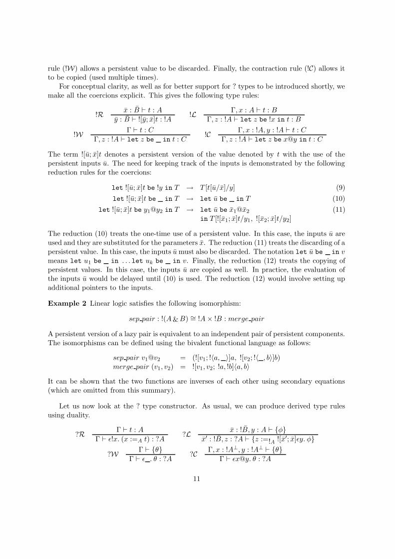
For conceptual clarity, as well as for better support for ? types to be introduced shortly, wemake all the coercions explicit. This gives the following type rules:

!Rx : B ` t : A

y : B ` ![y; x]t : !A!L

Γ, x : A ` t : B

Γ, z : !A ` let z be !x in t : B

!WΓ ` t : C

Γ, z : !A ` let z be in t : C!C

Γ, x : !A, y : !A ` t : C

Γ, z : !A ` let z be x@y in t : C

The term ![u; x]t denotes a persistent version of the value denoted by t with the use of thepersistent inputs u. The need for keeping track of the inputs is demonstrated by the followingreduction rules for the coercions:

let ![u; x]t be !y in T → T [t[u/x]/y] (9)

let ![u; x]t be in T → let u be in T (10)

let ![u; x]t be y1@y2 in T → let u be x1@x2

in T [![x1; x]t/y1, ![x2; x]t/y2](11)

The reduction (10) treats the one-time use of a persistent value. In this case, the inputs u areused and they are substituted for the parameters x. The reduction (11) treats the discarding of apersistent value. In this case, the inputs umust also be discarded. The notation let u be in vmeans let u1 be in . . . let uk be in v. Finally, the reduction (12) treats the copying ofpersistent values. In this case, the inputs u are copied as well. In practice, the evaluation ofthe inputs u would be delayed until (10) is used. The reduction (12) would involve setting upadditional pointers to the inputs.

Example 2 Linear logic satisfies the following isomorphism:

sep pair : !(A&B) ∼= !A× !B : merge pair

A persistent version of a lazy pair is equivalent to an independent pair of persistent components.The isomorphisms can be defined using the bivalent functional language as follows:

sep pair v1@v2 = (![v1; !〈a, 〉]a, ![v2; !〈 , b〉]b)merge pair (v1, v2) = ![v1, v2; !a, !b]〈a, b〉

It can be shown that the two functions are inverses of each other using secondary equations(which are omitted from this summary).

Let us now look at the ? type constructor. As usual, we can produce derived type rulesusing duality.

?RΓ ` t : A

Γ ` ε!x. (x :=A t) : ?A?L

x : !B, y : A ` {φ}

x′ : !B, z : ?A ` {z :=!A ![x′; x]εy. φ}

?WΓ ` {θ}

Γ ` ε . θ : ?A?C

Γ, x : !A⊥, y : !A⊥ ` {θ}Γ ` εx@y. θ : ?A

11

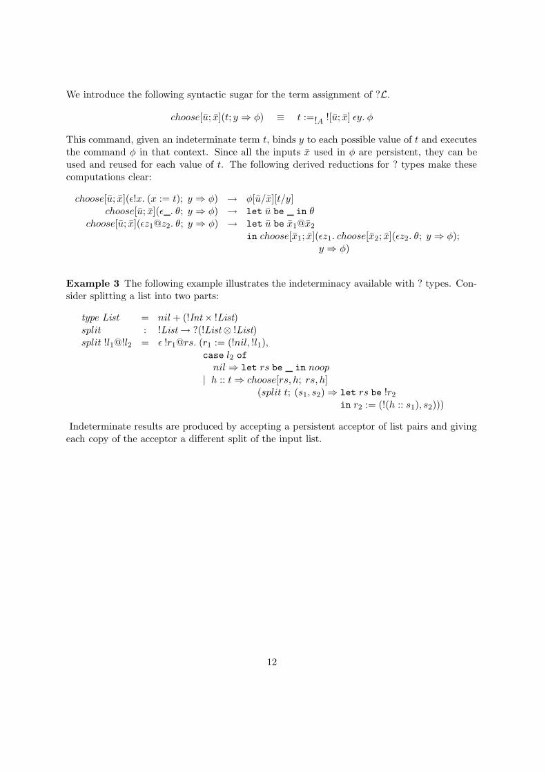
We introduce the following syntactic sugar for the term assignment of ?L.

choose[u; x](t; y ⇒ φ) ≡ t :=!A ![u; x] εy. φ

This command, given an indeterminate term t, binds y to each possible value of t and executesthe command φ in that context. Since all the inputs x used in φ are persistent, they can beused and reused for each value of t. The following derived reductions for ? types make thesecomputations clear:

choose[u; x](ε!x. (x := t); y ⇒ φ) → φ[u/x][t/y]choose[u; x](ε . θ; y ⇒ φ) → let u be in θ

choose[u; x](εz1@z2. θ; y ⇒ φ) → let u be x1@x2

in choose[x1; x](εz1. choose[x2; x](εz2. θ; y ⇒ φ);y ⇒ φ)

Example 3 The following example illustrates the indeterminacy available with ? types. Con-sider splitting a list into two parts:

type List = nil + (!Int × !List)split : !List → ?(!List ⊗ !List)split !l1@!l2 = ε !r1@rs. (r1 := (!nil, !l1),

case l2 ofnil ⇒ let rs be in noop

| h :: t⇒ choose[rs, h; rs, h](split t; (s1, s2) ⇒ let rs be !r2

in r2 := (!(h :: s1), s2)))

Indeterminate results are produced by accepting a persistent acceptor of list pairs and givingeach copy of the acceptor a different split of the input list.

12

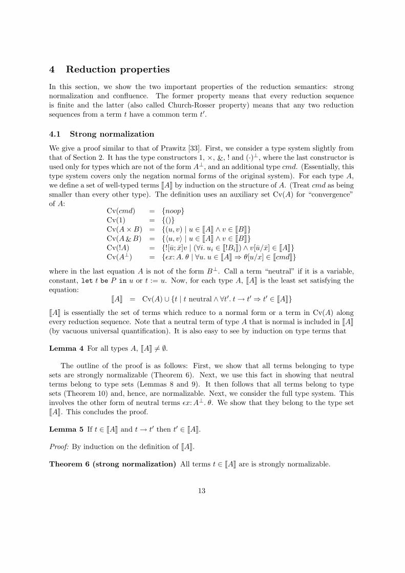
4 Reduction properties

In this section, we show the two important properties of the reduction semantics: strongnormalization and confluence. The former property means that every reduction sequenceis finite and the latter (also called Church-Rosser property) means that any two reductionsequences from a term t have a common term t′.

4.1 Strong normalization

We give a proof similar to that of Prawitz [33]. First, we consider a type system slightly fromthat of Section 2. It has the type constructors 1, ×, &, ! and (·)⊥, where the last constructor isused only for types which are not of the form A⊥, and an additional type cmd. (Essentially, thistype system covers only the negation normal forms of the original system). For each type A,we define a set of well-typed terms [[A]] by induction on the structure of A. (Treat cmd as beingsmaller than every other type). The definition uses an auxiliary set Cv(A) for “convergence”of A:

Cv(cmd) = {noop}Cv(1) = {()}Cv(A×B) = {(u, v) | u ∈ [[A]] ∧ v ∈ [[B]]}Cv(A&B) = {〈u, v〉 | u ∈ [[A]] ∧ v ∈ [[B]]}Cv(!A) = {![u; x]v | (∀i. ui ∈ [[!Bi]]) ∧ v[u/x] ∈ [[A]]}Cv(A⊥) = {εx:A. θ | ∀u. u ∈ [[A]] ⇒ θ[u/x] ∈ [[cmd]]}

where in the last equation A is not of the form B⊥. Call a term “neutral” if it is a variable,constant, let t be P in u or t := u. Now, for each type A, [[A]] is the least set satisfying theequation:

[[A]] = Cv(A) ∪ {t | t neutral ∧ ∀t′. t→ t′ ⇒ t′ ∈ [[A]]}

[[A]] is essentially the set of terms which reduce to a normal form or a term in Cv(A) alongevery reduction sequence. Note that a neutral term of type A that is normal is included in [[A]](by vacuous universal quantification). It is also easy to see by induction on type terms that

Lemma 4 For all types A, [[A]] 6= ∅.

The outline of the proof is as follows: First, we show that all terms belonging to typesets are strongly normalizable (Theorem 6). Next, we use this fact in showing that neutralterms belong to type sets (Lemmas 8 and 9). It then follows that all terms belong to typesets (Theorem 10) and, hence, are normalizable. Next, we consider the full type system. Thisinvolves the other form of neutral terms εx:A⊥. θ. We show that they belong to the type set[[A]]. This concludes the proof.

Lemma 5 If t ∈ [[A]] and t→ t′ then t′ ∈ [[A]].

Proof: By induction on the definition of [[A]].

Theorem 6 (strong normalization) All terms t ∈ [[A]] are is strongly normalizable.

13

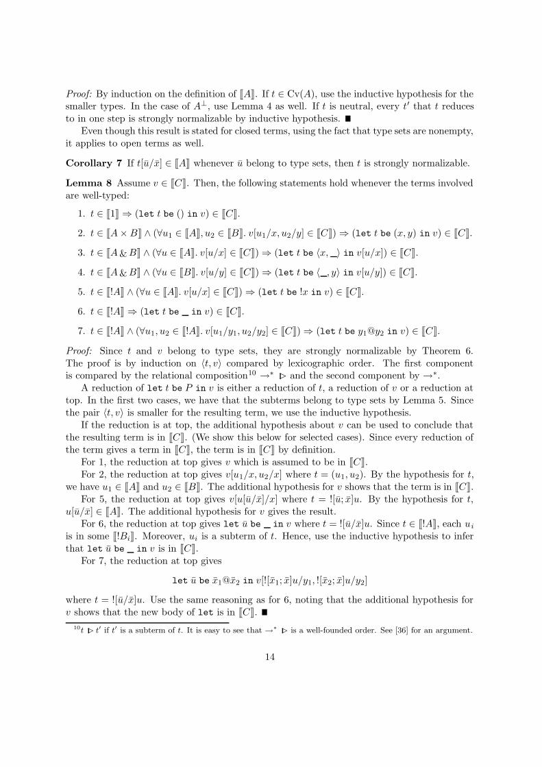
Proof: By induction on the definition of [[A]]. If t ∈ Cv(A), use the inductive hypothesis for thesmaller types. In the case of A⊥, use Lemma 4 as well. If t is neutral, every t′ that t reducesto in one step is strongly normalizable by inductive hypothesis.

Even though this result is stated for closed terms, using the fact that type sets are nonempty,it applies to open terms as well.

Corollary 7 If t[u/x] ∈ [[A]] whenever u belong to type sets, then t is strongly normalizable.

Lemma 8 Assume v ∈ [[C]]. Then, the following statements hold whenever the terms involvedare well-typed:

1. t ∈ [[1]] ⇒ (let t be () in v) ∈ [[C]].

2. t ∈ [[A×B]] ∧ (∀u1 ∈ [[A]], u2 ∈ [[B]]. v[u1/x, u2/y] ∈ [[C]]) ⇒ (let t be (x, y) in v) ∈ [[C]].

3. t ∈ [[A&B]] ∧ (∀u ∈ [[A]]. v[u/x] ∈ [[C]]) ⇒ (let t be 〈x, 〉 in v[u/x]) ∈ [[C]].

4. t ∈ [[A&B]] ∧ (∀u ∈ [[B]]. v[u/y] ∈ [[C]]) ⇒ (let t be 〈 , y〉 in v[u/y]) ∈ [[C]].

5. t ∈ [[!A]] ∧ (∀u ∈ [[A]]. v[u/x] ∈ [[C]]) ⇒ (let t be !x in v) ∈ [[C]].

6. t ∈ [[!A]] ⇒ (let t be in v) ∈ [[C]].

7. t ∈ [[!A]] ∧ (∀u1, u2 ∈ [[!A]]. v[u1/y1, u2/y2] ∈ [[C]]) ⇒ (let t be y1@y2 in v) ∈ [[C]].

Proof: Since t and v belong to type sets, they are strongly normalizable by Theorem 6.The proof is by induction on 〈t, v〉 compared by lexicographic order. The first componentis compared by the relational composition10 →∗ > and the second component by →∗.

A reduction of let t be P in v is either a reduction of t, a reduction of v or a reduction attop. In the first two cases, we have that the subterms belong to type sets by Lemma 5. Sincethe pair 〈t, v〉 is smaller for the resulting term, we use the inductive hypothesis.

If the reduction is at top, the additional hypothesis about v can be used to conclude thatthe resulting term is in [[C]]. (We show this below for selected cases). Since every reduction ofthe term gives a term in [[C]], the term is in [[C]] by definition.

For 1, the reduction at top gives v which is assumed to be in [[C]].For 2, the reduction at top gives v[u1/x, u2/x] where t = (u1, u2). By the hypothesis for t,

we have u1 ∈ [[A]] and u2 ∈ [[B]]. The additional hypothesis for v shows that the term is in [[C]].For 5, the reduction at top gives v[u[u/x]/x] where t = ![u; x]u. By the hypothesis for t,

u[u/x] ∈ [[A]]. The additional hypothesis for v gives the result.For 6, the reduction at top gives let u be in v where t = ![u/x]u. Since t ∈ [[!A]], each ui

is in some [[!Bi]]. Moreover, ui is a subterm of t. Hence, use the inductive hypothesis to inferthat let u be in v is in [[C]].

For 7, the reduction at top gives

let u be x1@x2 in v[![x1; x]u/y1, ![x2; x]u/y2]

where t = ![u/x]u. Use the same reasoning as for 6, noting that the additional hypothesis forv shows that the new body of let is in [[C]].

10t > t

′ if t′ is a subterm of t. It is easy to see that →∗

> is a well-founded order. See [36] for an argument.

14

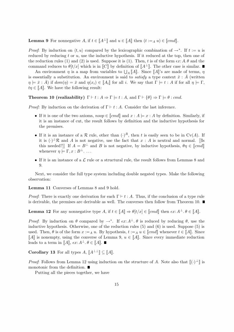
Lemma 9 For nonnegative A, if t ∈ [[A⊥]] and u ∈ [[A]] then (t :=A u) ∈ [[cmd]].

Proof: By induction on 〈t, u〉 compared by the lexicographic combination of →∗. If t := u isreduced by reducing t or u, use the inductive hypothesis. If it reduced at the top, then one ofthe reduction rules (1) and (2) is used. Suppose it is (1). Then, t is of the form εx:A.θ and thecommand reduces to θ[t/x] which is in [[C]] by definition of [[A⊥]]. The other case is similar.

An environment η is a map from variables to⋃

A [[A]]. Since [[A]]’s are made of terms, ηis essentially a substitution. An environment is said to satisfy a type context x : A (writtenη |= x : A) if dom(η) = x and η(xi) ∈ [[Ai]] for all i. We say that Γ |= t : A if for all η |= Γ,tη ∈ [[A]]. We have the following result:

Theorem 10 (realizability) Γ ` t : A⇒ Γ |= t : A, and Γ ` {θ} ⇒ Γ |= θ : cmd.

Proof: By induction on the derivation of Γ ` t : A. Consider the last inference.

• If it is one of the two axioms, noop ∈ [[cmd]] and x : A |= x : A by definition. Similarly, ifit is an instance of cut, the result follows by definition and the inductive hypothesis forthe premises.

• If it is an instance of a R rule, other than (·)R, then t is easily seen to be in Cv(A). Ifit is (·)⊥R and A is not negative, use the fact that x : A is neutral and normal. [[Isthis needed?]] If A = B⊥ and B is not negative, by inductive hypothesis, θη ∈ [[cmd]]whenever η |= Γ, x : B⊥. . . .

• If it is an instance of a L rule or a structural rule, the result follows from Lemmas 8 and9.

Next, we consider the full type system including double negated types. Make the followingobservation:

Lemma 11 Converses of Lemmas 8 and 9 hold.

Proof: There is exactly one derivation for each Γ ` t : A. Thus, if the conclusion of a type ruleis derivable, the premises are derivable as well. The converses then follow from Theorem 10.

Lemma 12 For any nonnegative type A, if t ∈ [[A]] ⇒ θ[t/x] ∈ [[cmd]] then εx:A⊥. θ ∈ [[A]].

Proof: By induction on θ compared by →∗. If εx:A⊥. θ is reduced by reducing θ, use theinductive hypothesis. Otherwise, one of the reduction rules (5) and (6) is used. Suppose (5) isused. Then, θ is of the form x :=A u. By hypothesis, t :=A u ∈ [[cmd]] whenever t ∈ [[A]]. Since[[A]] is nonempty, using the converse of Lemma 9, u ∈ [[A]]. Since every immediate reductionleads to a term in [[A]], εx:A⊥. θ ∈ [[A]].

Corollary 13 For all types A, [[A⊥⊥]] ⊆ [[A]].

Proof: Follows from Lemma 12 using induction on the structure of A. Note also that [[(·)⊥]] ismonotonic from the definition.

Putting all the pieces together, we have

15

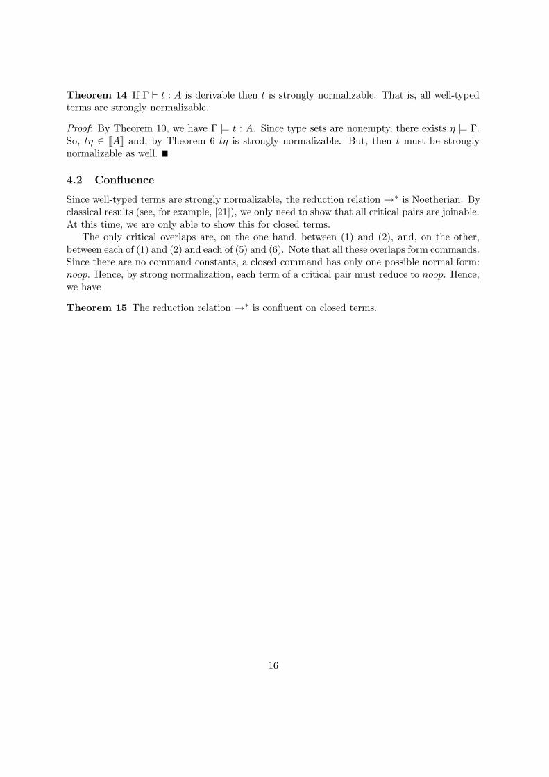
Theorem 14 If Γ ` t : A is derivable then t is strongly normalizable. That is, all well-typedterms are strongly normalizable.

Proof: By Theorem 10, we have Γ |= t : A. Since type sets are nonempty, there exists η |= Γ.So, tη ∈ [[A]] and, by Theorem 6 tη is strongly normalizable. But, then t must be stronglynormalizable as well.

4.2 Confluence

Since well-typed terms are strongly normalizable, the reduction relation →∗ is Noetherian. Byclassical results (see, for example, [21]), we only need to show that all critical pairs are joinable.At this time, we are only able to show this for closed terms.

The only critical overlaps are, on the one hand, between (1) and (2), and, on the other,between each of (1) and (2) and each of (5) and (6). Note that all these overlaps form commands.Since there are no command constants, a closed command has only one possible normal form:noop. Hence, by strong normalization, each term of a critical pair must reduce to noop. Hence,we have

Theorem 15 The reduction relation →∗ is confluent on closed terms.

16

5 Conclusion

We have shown that classical linear logic has significant applications to functional programmingwhich go considerably beyond the applications of linearity considered in previous work. Inparticular, it allows the design of typed functional languages which incorporate novel pro-gramming concepts such as first-class acceptor values. These values systematize and generalizesingle assignment variables, on the one hand, and continuations on the other. It also allows asystematic use of nondeterminism in functional programs.

For space limitations, we did not have adequate opportunity to comment on implementationaspects. Essentially, data flow languages, logic programming languages and continuationssuggest three different kinds of implementation paradigms with varying degrees of overheadsand concurrency. Perhaps, the most efficient paradigm for sequential implementations isthe model of logic programming where acceptors are implemented by unbound cells and areeventually filled by values.

Our main motivation in this study has been to better understand the issues of imperativeconcepts in functional languages [43, 42]. Single assignment variables represented by negativetypes are a particularly simple form of references. The insights obtained from this study shouldalso eventually lead to a better understanding of references.

Acknowledgments

I am indebted to Dick Kieburtz and Boris Agapiev for introducing me to the fascinating worldof linear logic. Thanks are also due to Sam Kamin and Vipin Swarup for several discussions.

17

References

[1] S. Abramsky. Computational Interpretations of Linear Logic. Research Report DOC90/20, Imperial College, London, Oct 1990.

[2] S. Abramsky and S. Vickers. Quantales, Observational Logic and Process Semantics.Research Report DOC 90/1, Imperial College, LOndon, Jan 1990.

[3] A. Asperti. A logic for concurrency. Unpublished manuscript, Nov. 1987.

[4] F. Bronsard and U. S. Reddy. An axiomatization of a functional logic language. InH. Kirchner and W. Wechler, editors, Algebraic and Logic Programming, pages 101–116,Springer-Verlag, 1990. (LNCS Vol. 463).

[5] C. Brown. Relating Petri Nets to Formulae of Linear Logic. Technical Report ECS-LFCS-89-87, University of Edinburgh, June 1989.

[6] K. L. Clark and S. A. Tarnlund. A first-order theory of data and programs. In Information

Processing, pages 939–944, North-Holland, 1977.

[7] W. F. Clocksin and C. S. Mellish. Programming in Prolog. Springer-Verlag, New York,1981.

[8] R. L. Constable, et. al. Implementing Mathematics with the Nuprl Proof Development

System. Prentice-Hall, New York, 1986.

[9] M. Felleisen, D. P. Friedman, E. Kohlbecker, and B. Duba. A syntactic theory of sequentialcontrol. Theoretical Comp. Science, 52(3):205–237, 1987. (to appear).

[10] A. Filinski. Linear continuations. In ACM Symp. on Princ. of Programming Languages,page (to appear), ACM, Alburquerque, New Mexico, Jan 1992.

[11] V. Gehlot and C. Gunter. Normal process representatives. In Symp. on Logic in Computer

Science, pages 200–207, IEEE, Philadelphia, Pa., June 1990.

[12] J.-Y. Girard. Linear logic. Theoretical Comp. Science, 50:1–102, 1987.

[13] J.-Y. Girard. Linear logic and parallelism. In M. V. Zilli, editor, Mathematical Models for

the Semantics of Parallelism, pages 166–182, Springer-Verlag, Berlin, 1987. (LNCS Vol.280).

[14] J.-Y. Girard. Towards a geometry of interaction. In J. W. Gray and A. Scedrov, editors,Categories in Computer Science and Logic, pages 69–108, American Mathematical Society,Boulder, Colorado, June 1987. (Contemporary Mathematics, Vol. 92).

[15] J-Y. Girard, Y. Lafont, and P. Taylor. Proofs and Types. Cambridge Tracts in Theor.

Comp. Science, Cambridge Univ. Press, Cambridge, 1989.

[16] S. Gregory. Parallel Logic Programming in PARLOG: The Language and its Implementa-

tion. International Series in Logic Programming, Addison-Wesley, Reading, Mass., 1987.

18

[17] T. G. Griffin. A formulae-as-types notion of control. In ACM Symp. on Princ. of

Programming Languages, pages 47–58, ACM, San Francisco, Jan 1990.

[18] D. Hilbert and W. Ackermann. Principles of Mathematical Logic. Chelsea Pub. Co., NewYork, 1950. translated by L. M. Hammond, G. G. Leckie, and F. Steinhardt.

[19] S. Holmstrom. A linear functional language. Draft paper, Chalmers University ofTechnology, 1988.

[20] W. A. Howard. The formulae-as-types notion of construction. In J. R. Hindley and J. P.Seldin, editors, To H. B. Curry: Essays on Combinatory Logic, Lambda Calculus and

Formalism, pages 479–490, Academic Press, New York, 1980.

[21] G. Huet. Confluent reductions: abstract properties and applications to term rewritingsystems. Journal of the ACM, 27(4):797–821, October 1980. (Previous version in Proc.

Symp. Foundations of Computer Science, Oct 1977).

[22] R. Jagadeesan, P. Panangaden, and K. Pingali. A fully abstract semantics for a functionallanguage with logic variables. In Fourth Ann. Symp. on Logic in Computer Science, page ,IEEE, 1989.

[23] Y. Lafont. Interaction nets. In Seventeenth Ann. ACM Symp. on Princ. of Programming

Languages, pages 95–108, ACM, San Francisco, Ca., Jan 1990.

[24] Y. Lafont. The linear abstract machine. Theoretical Comp. Science, 59:157–180, 1988.

[25] G. Lindstrom. Functional programming and the logical variable. In ACM Symp. on Princ.

of Programming Languages, 1985.

[26] D. MacQueen. Modules for Standard ML. In ACM Symp. on LISP and Functional

Programming, pages 198–207, 1984. (Revised version in Polymorphism Newsletter, II,2, Oct 85.

[27] P. Martin-Lof. Constructive mathematics and computer programming. In L. J. Cohen,J. Los, H. Pfeiffer, and K.-P. Podewski, editors, Proc. Sixth Intern. Congress for Logic,

Methodology and Philosophy of Science, pages 153–175, North-Holland, Amsterdam, 1982.

[28] N. Marti-Oliet and J. Meseguer. From Petri nets to linear logic. Mathematical Structures

in Computer Science, 1:69–101, 1991.

[29] J. C. Mitchell and G. D. Plotkin. Abstract types have existential types. In ACM Symp.

on Princ. of Programming Languages, pages 37–51, January 1985.

[30] C. Murthy. An evaluation semantics for classical proofs. In Sixth Ann. Symp. on Logic in

Computer Science, pages 96–109, IEEE, Amsterdam, Jul 1991.

[31] C. Murthy. Extracting Constructive Content from Classical Proofs. PhD thesis, CornellUniversity, Aug 1990.

[32] R.S. Nikhil, K. Pingali, and Arvind. Id Nouveau. Technical Report CSG 265, MIT, 1986.

19

[33] D. Prawitz. Ideas and results in proof theory. In Proc. Second Scandinavian Logic

Symposium, Springer-Verlag, 1970.

[34] U. S. Reddy. Narrowing as the operational semantics of functional languages. In Symp.

on Logic Programming, pages 138–151, IEEE, Boston, 1985.

[35] U. S. Reddy. On the relationship between logic and functional languages. In D. DeGrootand G. Lindstrom, editors, Logic Programming: Functions, Relations and Equations,pages 3–36, Prentice-Hall, 1986.

[36] U. S. Reddy. Term rewriting induction. In M. Stickel, editor, 10th International Conference

on Automated Deduction, pages 162–177, Springer-Verlag, 1990. (Lecture Notes inArtificial Intelligence, Vol. 449).

[37] U. S. Reddy. Transformation of logic programs into functional programs. In Intern. Symp.

on Logic Programming, pages 187–197, IEEE, 1984.

[38] J. C. Reynolds. The essence of Algol. In J. W. de Bakker and J. C. van Vliet, editors,Algorithmic Languages, pages 345–372, North-Holland, 1981.

[39] J. C. Reynolds. Preliminary Design of the Programming Language Forsythe. TechnicalReport CMU-CS-88-159, Carnegie-Mellon University, June 1988.

[40] R. A. G. Seely. Linear logic, *-autonomous categories and cofree coalgebras. In J. W. Grayand A. Scedrov, editors, Proc. AMS-IMS-SIAM Joint Conf. on Categories in Computer

Science and Logic, pages 371–382, American Mathematical Society, Boulder, Colorado,1989. (Contemporary Mathematics, Vol. 92).

[41] L. Sterling and E. Shapiro. The Art of Prolog. MIT Press, Cambridge, Mass., 1986.

[42] V. Swarup and U. S. Reddy. A logical view of assignments. In M. J. O’Donnell, editor,Constructivity in Computer Science, pages 127–141, Trinity University, San Antonio,Texas, June 1991.

[43] V. Swarup, U. S. Reddy, and E. Ireland. Assignments for applicative languages. InR. J. M. Hughes, editor, Conf. on Functional Program. Lang. and Comput. Arch.,pages 192–214, Springer-Verlag, Berlin, 1991. (Earlier versions: University of Illinois atUrbana-Champaign, July 1990, Revised Nov 1990, Feb 1991).

[44] S. Thompson. Type Theory and Functional Programming. Addison-Wesley, Wokingham,England, 1991.

[45] P. Wadler. Is there a use for linear logic? In Proc. ACM SIGPLAN Conf. on Partial

Evaluation and Semantics-Based Program Manipulation, page , ACM, New York, 1991.(SIGPLAN Notices, to appear).

[46] P. Wadler. Linear types can change the world. In M. Broy and C. B. Jones, editors,Programming Concepts and Methods, page , North-Holland, Amsterdam, 1990. (Proc.IFIP TC 2 Working Conf., Sea of Galilee, Israel).

20

[47] D. Wakeling and C. Runciman. Linearity and laziness. In R. J. M. Hughes, editor, Conf.

on Functional Program. Lang. and Comput. Arch., pages 215–240, Springer-Verlag, Berlin,1991. (LNCS Vol. 523).

[48] D. H. D. Warren, L. M. Pereira, and F. Pereira. Prolog - the language and itsimplementation compared with Lisp. SIGPLAN Notices, 12(8), 1977.

21