Accelerating incompressible fluid flowsimulations using SIMD or GPU computing

Yushan Wang1, Marc Baboulin1,2,Yann Fraigneau1,3, Olivier Le Maıtre1,3, Karl Rupp4

1 Universite Paris-Sud, France2 INRIA, France3 CNRS, France

4 Argonne National Laboratory, USA

Yushan Wang, LRI Navier-Stokes Solver 1/27

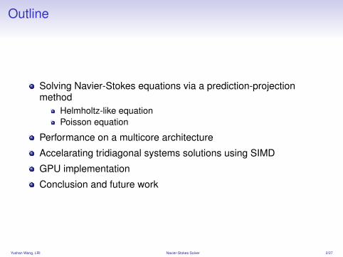
Outline

Solving Navier-Stokes equations via a prediction-projectionmethod

Helmholtz-like equationPoisson equation

Performance on a multicore architecture

Accelarating tridiagonal systems solutions using SIMD

GPU implementation

Conclusion and future work

Yushan Wang, LRI Navier-Stokes Solver 2/27

Navier-Stokes equationsThe Navier-Stokes equations describe mainly the motion of a viscousflow at all scales.

A Millennium Prize Problem of Navier-Stokes Euqations.http://www.claymath.org/millennium/Navier-Stokes_Equations/

Global Climate Models and the Navier-StokesEquations.http://climateaudit.org/2005/12/22/gcms-and-the-navier-stokes-equations/

Navier-Stokes simulation for the flow field around the Falcon business jet.http://mfquant.net/gallery_cfd.html

Yushan Wang, LRI Navier-Stokes Solver 3/27

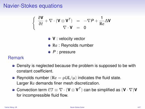
Navier-Stokes equations

{∂V∂t

+∇ · (V⊗ VT ) = −∇P +1

Re∆V

∇ · V = 0

V : velocity vector

Re : Reynolds number

P : pressureRemark

Density is neglected because the problem is supposed to be withconstant coefficient.

Reynolds number (Re = ρUL/µ) indicates the fluid state.Larger Re demands finer mesh discretization.

Convection term CT ≡ ∇ · (V⊗ VT ) can be simplified as (V · ∇)Vfor incompressible fluid flow.

Yushan Wang, LRI Navier-Stokes Solver 4/27

Numerical method

Finite difference method with staggered mesh. (V = (u, v)T )

v

i,j+1

u

i,j+1

v

i,j

v

i-1,j

v

i,j-1

v

i+1,j

u

i+1,ju

i,ju

i-1,j

u

i,j-1

of v

ontrol

volume

of u

mesh

element

volume

ontrol

x

i,j+1

x

i+1,jx

i,jx

i-1,j

x

i+1,j+1

x

i-1,j+1

x

i,j-1 x

i+1,j-1x

i-1,j-1

Yushan Wang, LRI Navier-Stokes Solver 5/27

Prediction-projection method3Vn+1 − 4Vn + Vn−1

2∆t+ CT

n+1= −∇Pn+1 +

1Re∆Vn+1 (0)

Hodge-Helmholtz decomposition: V∗ = Vn+1 +∇ψ

Prediction:3V∗ − 4Vn + Vn−1

2∆t+ CT

n+1= −∇Pn +

1Re∆V∗ (1)

Correction:3Vn+1 − 3V∗

2∆t= −∇(Pn+1 − Pn) +

1Re∆(Vn+1 − V∗)

(2)

(1) + 1Re∆Vn − 1

Re∆Vn =⇒ incremental Helmholtz-like

equation: (I −2∆t

31

Re∆)(V∗ − Vn) = S (3)

where S = 2∆t3 ( 1

Re∆Vn − CTn+1

−∇Pn) + Vn−Vn−1

3

∇ · (2) =⇒ Poisson equation: ∆φ =3

2∆t∇ · V∗ (4)

where φ = Pn+1 − Pn +1

Re∇ · V∗

Yushan Wang, LRI Navier-Stokes Solver 6/27

Prediction-projection method3Vn+1 − 4Vn + Vn−1

2∆t+ CT

n+1= −∇Pn+1 +

1Re∆Vn+1 (0)

Hodge-Helmholtz decomposition: V∗ = Vn+1 +∇ψ

Prediction:3V∗ − 4Vn + Vn−1

2∆t+ CT

n+1= −∇Pn +

1Re∆V∗ (1)

Correction:3Vn+1 − 3V∗

2∆t= −∇(Pn+1 − Pn) +

1Re∆(Vn+1 − V∗)

(2)

(1) + 1Re∆Vn − 1

Re∆Vn =⇒ incremental Helmholtz-like

equation: (I −2∆t

31

Re∆)(V∗ − Vn) = S (3)

where S = 2∆t3 ( 1

Re∆Vn − CTn+1

−∇Pn) + Vn−Vn−1

3

∇ · (2) =⇒ Poisson equation: ∆φ =3

2∆t∇ · V∗ (4)

where φ = Pn+1 − Pn +1

Re∇ · V∗

Yushan Wang, LRI Navier-Stokes Solver 6/27

Prediction-projection method3Vn+1 − 4Vn + Vn−1

2∆t+ CT

n+1= −∇Pn+1 +

1Re∆Vn+1 (0)

Hodge-Helmholtz decomposition: V∗ = Vn+1 +∇ψ

Prediction:3V∗ − 4Vn + Vn−1

2∆t+ CT

n+1= −∇Pn +

1Re∆V∗ (1)

Correction:3Vn+1 − 3V∗

2∆t= −∇(Pn+1 − Pn) +

1Re∆(Vn+1 − V∗)

(2)

(1) + 1Re∆Vn − 1

Re∆Vn =⇒ incremental Helmholtz-like

equation: (I −2∆t

31

Re∆)(V∗ − Vn) = S (3)

where S = 2∆t3 ( 1

Re∆Vn − CTn+1

−∇Pn) + Vn−Vn−1

3

∇ · (2) =⇒ Poisson equation: ∆φ =3

2∆t∇ · V∗ (4)

where φ = Pn+1 − Pn +1

Re∇ · V∗

Yushan Wang, LRI Navier-Stokes Solver 6/27

Prediction-projection method3Vn+1 − 4Vn + Vn−1

2∆t+ CT

n+1= −∇Pn+1 +

1Re∆Vn+1 (0)

Hodge-Helmholtz decomposition: V∗ = Vn+1 +∇ψ

Prediction:3V∗ − 4Vn + Vn−1

2∆t+ CT

n+1= −∇Pn +

1Re∆V∗ (1)

Correction:3Vn+1 − 3V∗

2∆t= −∇(Pn+1 − Pn) +

1Re∆(Vn+1 − V∗)

(2)

(1) + 1Re∆Vn − 1

Re∆Vn =⇒ incremental Helmholtz-like

equation: (I −2∆t

31

Re∆)(V∗ − Vn) = S (3)

where S = 2∆t3 ( 1

Re∆Vn − CTn+1

−∇Pn) + Vn−Vn−1

3

∇ · (2) =⇒ Poisson equation: ∆φ =3

2∆t∇ · V∗ (4)

where φ = Pn+1 − Pn +1

Re∇ · V∗

Yushan Wang, LRI Navier-Stokes Solver 6/27

Prediction-projection method3Vn+1 − 4Vn + Vn−1

2∆t+ CT

n+1= −∇Pn+1 +

1Re∆Vn+1 (0)

Hodge-Helmholtz decomposition: V∗ = Vn+1 +∇ψ

Prediction:3V∗ − 4Vn + Vn−1

2∆t+ CT

n+1= −∇Pn +

1Re∆V∗ (1)

Correction:3Vn+1 − 3V∗

2∆t= −∇(Pn+1 − Pn) +

1Re∆(Vn+1 − V∗)

(2)

(1) + 1Re∆Vn − 1

Re∆Vn =⇒ incremental Helmholtz-like

equation: (I −2∆t

31

Re∆)(V∗ − Vn) = S (3)

where S = 2∆t3 ( 1

Re∆Vn − CTn+1

−∇Pn) + Vn−Vn−1

3

∇ · (2) =⇒ Poisson equation: ∆φ =3

2∆t∇ · V∗ (4)

where φ = Pn+1 − Pn +1

Re∇ · V∗

Yushan Wang, LRI Navier-Stokes Solver 6/27

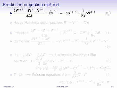
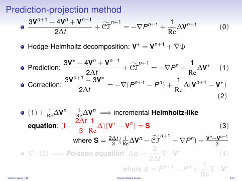
Prediction-projection method3Vn+1 − 4Vn + Vn−1

2∆t+ CT

n+1= −∇Pn+1 +

1Re∆Vn+1 (0)

Hodge-Helmholtz decomposition: V∗ = Vn+1 +∇ψ

Prediction:3V∗ − 4Vn + Vn−1

2∆t+ CT

n+1= −∇Pn +

1Re∆V∗ (1)

Correction:3Vn+1 − 3V∗

2∆t= −∇(Pn+1 − Pn) +

1Re∆(Vn+1 − V∗)

(2)

(1) + 1Re∆Vn − 1

Re∆Vn =⇒ incremental Helmholtz-like

equation: (I −2∆t

31

Re∆)(V∗ − Vn) = S (3)

where S = 2∆t3 ( 1

Re∆Vn − CTn+1

−∇Pn) + Vn−Vn−1

3

∇ · (2) =⇒ Poisson equation: ∆φ =3

2∆t∇ · V∗ (4)

where φ = Pn+1 − Pn +1

Re∇ · V∗

Yushan Wang, LRI Navier-Stokes Solver 6/27

Prediction-projection method

Time increment on V and P:Pn+1 = Pn + φ−

1Re∇ · V∗

Vn+1 = V∗ −2∆t

3∇φ

Time iterations:

Pn

Vn

}=⇒

Helmholtz−like eq.V∗ =⇒

Poisson eq.φ =⇒

Increments

{Pn+1

Vn+1

Yushan Wang, LRI Navier-Stokes Solver 7/27

Solving Helmholtz-like equation with ADI method

(I −2∆t

31

Re∆)(V∗i − Vn

i ) = Si i ∈ {x , y , z}

Alternating Direction Implicit methodThe 3D operator (I − ε∆) is approximated as a product of three 1Doperators:

I − ε∆ = (I − ε∆x)(I − ε∆y)(I − ε∆z) + O(ε2)

(I −2∆t

31

Re∆x)T′ = S

(I −2∆t

31

Re∆y)T′′ = T′ i ∈ {x , y , z}

(I −2∆t

31

Re∆z)(V∗i − Vn

i ) = T′′

Yushan Wang, LRI Navier-Stokes Solver 8/27

Solving Helmholtz-like equation with ADI method

(I −2∆t

31

Re∆)(V∗i − Vn

i ) = Si i ∈ {x , y , z}

Alternating Direction Implicit methodThe 3D operator (I − ε∆) is approximated as a product of three 1Doperators:

I − ε∆ = (I − ε∆x)(I − ε∆y)(I − ε∆z) + O(ε2)

(I −2∆t

31

Re∆x)T′ = S

(I −2∆t

31

Re∆y)T′′ = T′ i ∈ {x , y , z}

(I −2∆t

31

Re∆z)(V∗i − Vn

i ) = T′′

Yushan Wang, LRI Navier-Stokes Solver 8/27

Solving Helmholtz-like equation with ADI method

(I −2∆t

31

Re∆)(V∗i − Vn

i ) = Si i ∈ {x , y , z}

Alternating Direction Implicit methodThe 3D operator (I − ε∆) is approximated as a product of three 1Doperators:

I − ε∆ = (I − ε∆x)(I − ε∆y)(I − ε∆z) + O(ε2)

(I −2∆t

31

Re∆x)T′ = S

(I −2∆t

31

Re∆y)T′′ = T′ i ∈ {x , y , z}

(I −2∆t

31

Re∆z)(V∗i − Vn

i ) = T′′

Yushan Wang, LRI Navier-Stokes Solver 8/27

Block tridiagonal matrix

Matrix structure of (I −2∆t

31

Re∆x)

nx

nx

ny × nz blocks

Yushan Wang, LRI Navier-Stokes Solver 9/27

Solving Poisson equation using partial diagonalization

∆φ =3∇ · V∗

2∆t⇔ Lφ = S ⇔ (Lx + Ly + Lz)φ = S.

Lx = QxΛxQ−1x

Ly = QyΛy Q−1y

S′ = Q−1x Q−1

y S

φ′ = Q−1x Q−1

y φ

⇒ (Λx +Λy + Lz)φ

′ = S′

Projection of source term: S′ = Q−1x Q−1

y S

Solution of tridiagonal system: (Λx +Λy + Lz)φ′ = S′

Final solution is: φ = Qy Qxφ′

Remark: this method is only available for separable problems.

Yushan Wang, LRI Navier-Stokes Solver 10/27

Solving Poisson equation using partial diagonalization

∆φ =3∇ · V∗

2∆t⇔ Lφ = S ⇔ (Lx + Ly + Lz)φ = S.

Lx = QxΛxQ−1x

Ly = QyΛy Q−1y

S′ = Q−1x Q−1

y S

φ′ = Q−1x Q−1

y φ

⇒ (Λx +Λy + Lz)φ

′ = S′

Projection of source term: S′ = Q−1x Q−1

y S

Solution of tridiagonal system: (Λx +Λy + Lz)φ′ = S′

Final solution is: φ = Qy Qxφ′

Remark: this method is only available for separable problems.

Yushan Wang, LRI Navier-Stokes Solver 10/27

Solving Poisson equation using partial diagonalization

∆φ =3∇ · V∗

2∆t⇔ Lφ = S ⇔ (Lx + Ly + Lz)φ = S.

Lx = QxΛxQ−1x

Ly = QyΛy Q−1y

S′ = Q−1x Q−1

y S

φ′ = Q−1x Q−1

y φ

⇒ (Λx +Λy + Lz)φ

′ = S′

Projection of source term: S′ = Q−1x Q−1

y S

Solution of tridiagonal system: (Λx +Λy + Lz)φ′ = S′

Final solution is: φ = Qy Qxφ′

Remark: this method is only available for separable problems.

Yushan Wang, LRI Navier-Stokes Solver 10/27

Solving Poisson equation using partial diagonalization

∆φ =3∇ · V∗

2∆t⇔ Lφ = S ⇔ (Lx + Ly + Lz)φ = S.

Lx = QxΛxQ−1x

Ly = QyΛy Q−1y

S′ = Q−1x Q−1

y S

φ′ = Q−1x Q−1

y φ

⇒ (Λx +Λy + Lz)φ

′ = S′

Projection of source term: S′ = Q−1x Q−1

y S

Solution of tridiagonal system: (Λx +Λy + Lz)φ′ = S′

Final solution is: φ = Qy Qxφ′

Remark: this method is only available for separable problems.

Yushan Wang, LRI Navier-Stokes Solver 10/27

Solving Poisson equation using partial diagonalization

∆φ =3∇ · V∗

2∆t⇔ Lφ = S ⇔ (Lx + Ly + Lz)φ = S.

Lx = QxΛxQ−1x

Ly = QyΛy Q−1y

S′ = Q−1x Q−1

y S

φ′ = Q−1x Q−1

y φ

⇒ (Λx +Λy + Lz)φ

′ = S′

Projection of source term: S′ = Q−1x Q−1

y S

Solution of tridiagonal system: (Λx +Λy + Lz)φ′ = S′

Final solution is: φ = Qy Qxφ′

Remark: this method is only available for separable problems.

Yushan Wang, LRI Navier-Stokes Solver 10/27

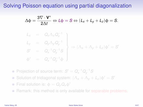
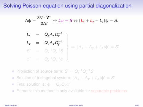
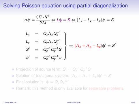
Solving Poisson equation using partial diagonalization

∆φ =3∇ · V∗

2∆t⇔ Lφ = S ⇔ (Lx + Ly + Lz)φ = S.

Lx = QxΛxQ−1x

Ly = QyΛy Q−1y

S′ = Q−1x Q−1

y S

φ′ = Q−1x Q−1

y φ

⇒ (Λx +Λy + Lz)φ

′ = S′

Projection of source term: S′ = Q−1x Q−1

y S

Solution of tridiagonal system: (Λx +Λy + Lz)φ′ = S′

Final solution is: φ = Qy Qxφ′

Remark: this method is only available for separable problems.

Yushan Wang, LRI Navier-Stokes Solver 10/27

Block tridiagonal matrixMatrix structure of (Λx +Λy + Lz)

nz

nz

ny × nx blocks

Yushan Wang, LRI Navier-Stokes Solver 11/27

Parallel implementation

������������������������������������������������������������������������������������������������������������������������������������������������������������������������

������������������������������������������������������������������������������������������������������������������������������������������������������������������������

����������������������������������������������������������������������������������������������������������������������������������������������������������

����������������������������������������������������������������������������������������������������������������������������������������������������������

������������������������������������������������������������������������������������������������������������������������������������������������������������������������

������������������������������������������������������������������������������������������������������������������������������������������������������������������������

����������������������������������������������������������������������������������������������������������������������������������������������������������

����������������������������������������������������������������������������������������������������������������������������������������������������������

IV

IV

I II

III

Domain decomposition viaSchur complement method.

Interface exchanges via MPI.

One subdomain corresponds toone process.

Kernels from ScaLAPACK andMKL libraries.

Yushan Wang, LRI Navier-Stokes Solver 12/27

Schur complement method

The Schur complement method is applied when there are multiplesubdomains along the solving direction.

I1

I2

y

z

x

Example for solving a tridiagonal systemalong z-direction.

This method results in information exchanges!

Yushan Wang, LRI Navier-Stokes Solver 13/27

Schur complement method

The Schur complement method is applied when there are multiplesubdomains along the solving direction.

I1

I2

y

z

x

Example for solving a tridiagonal systemalong z-direction.

This method results in information exchanges!

Yushan Wang, LRI Navier-Stokes Solver 13/27

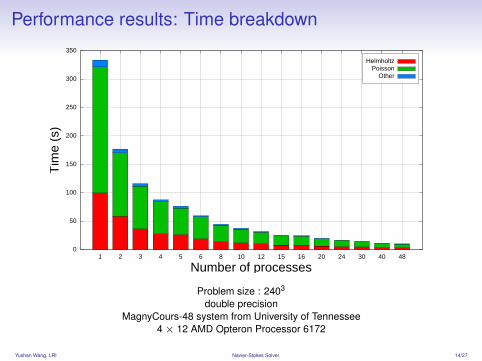
Performance results: Time breakdown

0

50

100

150

200

250

300

350

1 2 3 4 5 6 8 10 12 15 16 20 24 30 40 48

Tim

e (s

)

Number of processes

HelmholtzPoisson

Other

Problem size : 2403

double precisionMagnyCours-48 system from University of Tennessee

4× 12 AMD Opteron Processor 6172

Yushan Wang, LRI Navier-Stokes Solver 14/27

Performance results: Strong scalability

0

5

10

15

20

25

30

35

40

45

50

0 5 10 15 20 25 30 35 40 45 50

Spee

dup

Number of processes

CPUHelmholtz

PoissonIdeal

Problem size : 2403

double precisionMagnyCours-48 system from University of Tennessee

4× 12 AMD Opteron Processor 6172

Yushan Wang, LRI Navier-Stokes Solver 15/27

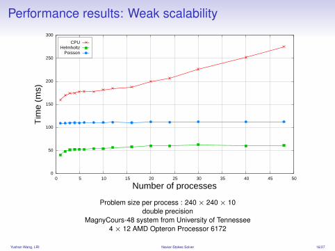
Performance results: Weak scalability

0

50

100

150

200

250

300

0 5 10 15 20 25 30 35 40 45 50

Tim

e (m

s)

Number of processes

CPUHelmholtz

Poisson

Problem size per process : 240× 240× 10double precision

MagnyCours-48 system from University of Tennessee4× 12 AMD Opteron Processor 6172

Yushan Wang, LRI Navier-Stokes Solver 16/27

Tridiagonal Solver

At each time step, 10 tridiagonal systems to solve.

Helmholtz-like equation:

(I −2∆t

31

Re∆x)T′ = Si

(I −2∆t

31

Re∆y)T′′ = T′ i ∈ {x , y , z}

(I −2∆t

31

Re∆z)(V∗i − Vn

i ) = T′′

Poisson equation:

(Λx +Λy + Lz)φ′ = S′

Yushan Wang, LRI Navier-Stokes Solver 17/27

Tridiagonal Solver

The tridiagonal systems have the same block tridiagonal structure.

=⇒

Helmholtz-like equation:The tridiagonal blocks are identical =⇒ a smaller tridiagonal systemwith multiple RHS.Second order central difference scheme =⇒ diagonally dominantmatrix.

Yushan Wang, LRI Navier-Stokes Solver 18/27

Thomas Algorithm

b1 c1

a2 b2 c2. . . . . . . . .

ai bi ci. . . . . . . . .

an−1 bn−1 cn−1

an bn

x1

x2...xi...

xn−1

xn

=

s1

s2...si...

sn−1

sn

.

Forward eliminationfor i = 2 to n, do

bi = bi −ci−1 × ai

bi−1;

si = si −si−1 × ai

bi−1;

end

Backward subtitution:xn =

sn

bn;

for i = n − 1 to 1, do

xi =si − ci × xi+1

bi;

end

Yushan Wang, LRI Navier-Stokes Solver 19/27

Vectorization

Implemented using a generic SIMD abstraction library(BOOST.SIMD) for all SSEx variants and AVX.

Boost.SIMD, a C++ template library that simplifies the exploitationof SIMD hardware within a standard C++ programming model.

Scalable system that takes care of increasing wide of SIMDsystems (128 bits today, 512 bits in Intel Xeon Phi coprocessors).

See [ Esterie et al., Boost.SIMD: Generic Programming forportable SIMDization ] .

Yushan Wang, LRI Navier-Stokes Solver 20/27

Tridiagonal solver with vectorization

a6

R1=(a1, a2)

R2=(b1, b2)

b1 b2 b3

R1=(a1, b1)

R2=(a2, b2)b4 b5

Shuffle(R1, R2)

b6 b7 ...

a1 a2 a3 a4 a5 a7 ...

=c3a3

a4

c1

a2 c2

b3

b4

x11 x2

1

x12 x2

2

x13 x2

3

x14 x2

4

s13 s23

s14 s24

s11

s12

s21

s22

b1

b2

Yushan Wang, LRI Navier-Stokes Solver 21/27

Tridiagonal solver with vectorization

a6

R1=(a1, a2)

R2=(b1, b2)

b1 b2 b3

R1=(a1, b1)

R2=(a2, b2)b4 b5

Shuffle(R1, R2)

b6 b7 ...

a1 a2 a3 a4 a5 a7 ...

=c3a3

a4

c1

c2

x11 x2

1

x12 x2

2

x13 x2

3

x14 x2

4

s11

s12

s21

s22

b1

b2

b3

b4

s13

s14

s23

s24

Yushan Wang, LRI Navier-Stokes Solver 21/27

Tridiagonal solver with vectorization

a6

R1=(a1, a2)

R2=(b1, b2)

b1 b2 b3

R1=(a1, b1)

R2=(a2, b2)b4 b5

Shuffle(R1, R2)

b6 b7 ...

a1 a2 a3 a4 a5 a7 ...

=c3

c1

c2

x11 x2

1

x12 x2

2

x13 x2

3

x14 x2

4

s11

s12

s21

s22

b1

b2

b3

b4

s13

s14

s23

s24

Yushan Wang, LRI Navier-Stokes Solver 21/27

Tridiagonal solver with vectorization

a6

R1=(a1, a2)

R2=(b1, b2)

b1 b2 b3

R1=(a1, b1)

R2=(a2, b2)b4 b5

Shuffle(R1, R2)

b6 b7 ...

a1 a2 a3 a4 a5 a7 ...

=c3

c1

c2

s11

s12

s21

s22

b1

b2

b3

b4

s13

s14

s23

s24x14 x2

4

x23x1

3

x22x1

2

x21x1

1

Yushan Wang, LRI Navier-Stokes Solver 21/27

Performance: Cycle per value

10

20

30

40

50

60

70

1.0e+02 1.0e+03 1.0e+04 1.0e+05 1.0e+06

Cyc

le p

er v

alue

(c/v

)

Number of RHS

DGTSVvectorized Thomas

L2 cache sizeL3 cache size

Intel(R) Xeon(R) CPU E5645 @ 2.40GHzdouble precision

Yushan Wang, LRI Navier-Stokes Solver 22/27

Steps of NS solver

Domain initialization

Computation of eigen values and vectorsFor each time iteration:− Solve Helmhlotz equation− Solve Poisson equation− Variables increments− Record current numerical solution

Yushan Wang, LRI Navier-Stokes Solver 23/27

Steps of NS solver

Domain initialization

Computation of eigen values and vectorsFor each time iteration:− Solve Helmhlotz equation− Solve Poisson equation− Variables increments− Record current numerical solution

Yushan Wang, LRI Navier-Stokes Solver 23/27

Helmholtz-like equation

Tridiagonal block structure with identical blocks.

One GPU thread deals with one RHS value.

Data reordering after each solving step.

Poisson equation

Tridiagonal block structure with different blocks.

One GPU thread deals with one tridiagonal block.

Matrix-matrix multiplication.

Data reordering after each multiplication and solving step.

Yushan Wang, LRI Navier-Stokes Solver 24/27

Preliminary results

Helmholtz PoissonTransfers CPU→ GPU 0.416s 0.126sMatrix multiplication - 0.024sSolution reordering 0.014s 0.014sTridiagonal system solve 0.169s(9) 0.169s(1)Total/iteration GPU solver 1.569s 0.333sTotal/iteration CPU solver (48 cores) 3.21s 6.45s

Tesla C2075 (448 CUDA cores), mini-titan@lri

Matrix multiplication by DGEMM of MAGMA library

Transfers not included (needed only at the begining of the time itration)

Yushan Wang, LRI Navier-Stokes Solver 25/27

Conclusion

Scalable algorithm and CPU implementation of a 3DNavier-Stokes equations.

Tridiagonal solver acceleration using vectorization.

For discontinuous domains, we use an iterative method to solvethe Poisson equation. (SOR+multigrid)

GPU Helmholtz and Poisson solver.

Ongoing workMultiGPU solver for Navier-Stokes equations using partialdiagonalisation and ADI method. Collaboration with Argonne NationalLaboratory (Karl Rupp).

Yushan Wang, LRI Navier-Stokes Solver 26/27

Yushan Wang, LRI Navier-Stokes Solver 27/27