Accelerating Binary Genetic Algorithm Driven Missile ... · A.15 Low Fidelity, Single Precision...

Accelerating Binary Genetic Algorithm Driven Missile Design OptimizationRoutine with a CUDA Coded Six Degrees-Of-Freedom Simulator

by

Daniel Benton

A thesis submitted to the Graduate Faculty ofAuburn University

in partial fulfillment of therequirements for the Degree of

Master of Science

Auburn, AlabamaDecember 12, 2015

Keywords: CUDA, six-dof, GPU, degrees-of-freedom, simulation, optimization

Copyright 2015 by Daniel Benton

Approved by

Roy Hartfield, Walt and Virginia Woltosz Professor of Aerospace EngineeringBrian Thurow, W. Allen and Martha Reed Associate Professor of Aerospace Engineering

David Scarborough, Assistant Professor of Aerospace EngineeringGeorge Flowers,Professor of Mechanical Engineering, Dean of Graduate School

Abstract

Science and Engineering has benefited enormously from the advent of modern (digital)

computing. As technology continues to grow, computation capability becomes exponentially

faster, more reliable, and more efficient. While modeling and simulations have hurdled analy-

sis past many years of trial and error, they still are restricted by resources, even with modern

computing. Whether running Monte Carlo simulations, or optimizing missile designs, reduc-

ing run-time of simulations is still an ultimate goal, as faster results are better results. The

method considered in this research gives an ordinary computer something resembling the

power of a supercomputer.

Over the past decade, innovative processing architecture has been introduced to the

field of scientific computing, to improve the High Performance Computing (HPC) sector:

Compute Unified Device Architecture (CUDA). The architecture is designed to have high

Floating Point OperationS (FLOPS) throughput by efficiently performing calculations and

fetching data concurrently. This creates a situation in which the device spends the majority

of the time on computing by constantly crunching numbers instead of waiting on necessary

data. A CUDA implementation of a Six-Degrees-of-Freedom (DOF) simulator is used with

a Binary Genetic Algorithm and a routine which calculates missile flight properties, to

optimize missile design. The performance of which, exceeds that of the same code run

on high performance central processing units. The results presented are validation metrics,

performance metrics of simulator studies and Optimization studies, and future optimization

techniques.

ii

Acknowledgments

I would like to thank Dr. Roy Hartfield for helping me through my studies whilst re-

maining a great mentor; Dr. John Burkhalter for his guidance in Genetic Algorithm; Dr.

Peter Zipfel for providing the backbone for this research; Auburn University for the oppor-

tunity, environment, and what has become a great family. I would also like to express an

unimaginable amount of gratitude for my Mom, my Dad, Charlotte, Heather, my Fr-amily:

Hamilton, Ash, Rus, Stef, Tristen, Littleton, Corey, and HQ; as well as the rest of my im-

mediate family: The Jarretts and The Ballards.

Belief is one thing, but Conviction will stir the soul. So, find reverence with a trailing

desire – Convictions will waiver as Truths evolve. Hold steady; hope will ever be yours to

brandish.

”What you do is what the whole Universe is doing at the place you call here

and now; you are something that the whole Universe is doing, in the same way

that a wave is something that the whole ocean is doing. The real you is not a

puppet . . . which life pushes around. The real deep down you is the whole

Universe.”

–Alan Watts

iii

Table of Contents

Abstract . . . . . . . . . . . . . . . . . . . . . . . . . . . . . . . . . . . . . . . . . . . ii

Acknowledgments . . . . . . . . . . . . . . . . . . . . . . . . . . . . . . . . . . . . . . iii

List of Figures . . . . . . . . . . . . . . . . . . . . . . . . . . . . . . . . . . . . . . . viii

List of Tables . . . . . . . . . . . . . . . . . . . . . . . . . . . . . . . . . . . . . . . . xiv

1 Introduction . . . . . . . . . . . . . . . . . . . . . . . . . . . . . . . . . . . . . . 1

1.1 Background . . . . . . . . . . . . . . . . . . . . . . . . . . . . . . . . . . . . 1

1.1.1 Central Processing Units . . . . . . . . . . . . . . . . . . . . . . . . . 1

1.1.2 Graphics Processing Unit . . . . . . . . . . . . . . . . . . . . . . . . 2

1.2 Motivation . . . . . . . . . . . . . . . . . . . . . . . . . . . . . . . . . . . . . 4

1.3 Objective . . . . . . . . . . . . . . . . . . . . . . . . . . . . . . . . . . . . . 5

2 Software . . . . . . . . . . . . . . . . . . . . . . . . . . . . . . . . . . . . . . . . 7

2.1 Binary Genetic Algorithm . . . . . . . . . . . . . . . . . . . . . . . . . . . . 7

2.2 Aero-Design . . . . . . . . . . . . . . . . . . . . . . . . . . . . . . . . . . . . 9

2.3 Dr. Peter Zipfels Six Degrees-of-Freedom Simulation . . . . . . . . . . . . . 10

2.3.1 Numerical Methods . . . . . . . . . . . . . . . . . . . . . . . . . . . . 15

2.3.2 Environment . . . . . . . . . . . . . . . . . . . . . . . . . . . . . . . 16

2.3.3 Kinematics . . . . . . . . . . . . . . . . . . . . . . . . . . . . . . . . 18

2.3.4 Newton . . . . . . . . . . . . . . . . . . . . . . . . . . . . . . . . . . 20

2.3.5 Euler . . . . . . . . . . . . . . . . . . . . . . . . . . . . . . . . . . . . 21

2.3.6 Aerodynamics . . . . . . . . . . . . . . . . . . . . . . . . . . . . . . . 21

2.3.7 Propulsion . . . . . . . . . . . . . . . . . . . . . . . . . . . . . . . . . 23

2.3.8 Forces and Intercept . . . . . . . . . . . . . . . . . . . . . . . . . . . 24

2.4 Program Flow . . . . . . . . . . . . . . . . . . . . . . . . . . . . . . . . . . . 25

iv

3 Hardware . . . . . . . . . . . . . . . . . . . . . . . . . . . . . . . . . . . . . . . 26

3.1 Graphics Processing Unit Architecture . . . . . . . . . . . . . . . . . . . . . 26

3.1.1 Schedulers . . . . . . . . . . . . . . . . . . . . . . . . . . . . . . . . . 30

3.1.2 Memory Hierarchy . . . . . . . . . . . . . . . . . . . . . . . . . . . . 31

3.1.3 New Architecture Versions . . . . . . . . . . . . . . . . . . . . . . . . 31

4 CUDA Implementation . . . . . . . . . . . . . . . . . . . . . . . . . . . . . . . . 33

4.1 Design . . . . . . . . . . . . . . . . . . . . . . . . . . . . . . . . . . . . . . . 33

4.2 Missile Structure . . . . . . . . . . . . . . . . . . . . . . . . . . . . . . . . . 33

4.3 Data Deck, Table, and Variable Structure . . . . . . . . . . . . . . . . . . . 36

4.4 CUDA Simulation . . . . . . . . . . . . . . . . . . . . . . . . . . . . . . . . . 38

5 Results . . . . . . . . . . . . . . . . . . . . . . . . . . . . . . . . . . . . . . . . . 41

5.1 Granularity Study . . . . . . . . . . . . . . . . . . . . . . . . . . . . . . . . . 41

5.1.1 The Setup . . . . . . . . . . . . . . . . . . . . . . . . . . . . . . . . . 41

5.1.2 Results . . . . . . . . . . . . . . . . . . . . . . . . . . . . . . . . . . . 41

5.1.3 Optimal Performance Trends . . . . . . . . . . . . . . . . . . . . . . 42

5.1.4 Validation . . . . . . . . . . . . . . . . . . . . . . . . . . . . . . . . . 43

5.1.5 Missile Design Study . . . . . . . . . . . . . . . . . . . . . . . . . . . 46

5.1.6 The Setup . . . . . . . . . . . . . . . . . . . . . . . . . . . . . . . . . 46

6 Conclusion . . . . . . . . . . . . . . . . . . . . . . . . . . . . . . . . . . . . . . . 49

6.1 The Goal . . . . . . . . . . . . . . . . . . . . . . . . . . . . . . . . . . . . . 49

6.2 Overcoming Obstacles . . . . . . . . . . . . . . . . . . . . . . . . . . . . . . 49

6.3 Conclusion of Results . . . . . . . . . . . . . . . . . . . . . . . . . . . . . . . 50

6.4 Future Work . . . . . . . . . . . . . . . . . . . . . . . . . . . . . . . . . . . . 51

6.4.1 Optimizations . . . . . . . . . . . . . . . . . . . . . . . . . . . . . . . 51

6.4.2 Moment of Inertia’s . . . . . . . . . . . . . . . . . . . . . . . . . . . . 53

6.4.3 Additional Vehicle Modules . . . . . . . . . . . . . . . . . . . . . . . 53

6.4.4 Closing . . . . . . . . . . . . . . . . . . . . . . . . . . . . . . . . . . . 54

v

Bibliography . . . . . . . . . . . . . . . . . . . . . . . . . . . . . . . . . . . . . . . . 55

A Thread Granularity Study Results . . . . . . . . . . . . . . . . . . . . . . . . . . 56

A.1 Granularity Effects . . . . . . . . . . . . . . . . . . . . . . . . . . . . . . . . 56

A.1.1 240 Missiles . . . . . . . . . . . . . . . . . . . . . . . . . . . . . . . . 56

A.1.2 480 Missiles . . . . . . . . . . . . . . . . . . . . . . . . . . . . . . . . 64

A.1.3 960 Missiles . . . . . . . . . . . . . . . . . . . . . . . . . . . . . . . . 72

A.1.4 1440 Missiles . . . . . . . . . . . . . . . . . . . . . . . . . . . . . . . 80

A.2 Optimal Performance Trends . . . . . . . . . . . . . . . . . . . . . . . . . . . 88

A.2.1 Double Precision . . . . . . . . . . . . . . . . . . . . . . . . . . . . . 88

A.2.2 Single Precision . . . . . . . . . . . . . . . . . . . . . . . . . . . . . . 92

B Optimization Study Results . . . . . . . . . . . . . . . . . . . . . . . . . . . . . 96

B.1 Results: CPU Convergence . . . . . . . . . . . . . . . . . . . . . . . . . . . . 96

B.2 Results: GPU Convergence . . . . . . . . . . . . . . . . . . . . . . . . . . . . 103

C Setting up CUDA on Windows . . . . . . . . . . . . . . . . . . . . . . . . . . . 109

C.1 Installing CUDA Toolkit . . . . . . . . . . . . . . . . . . . . . . . . . . . . . 109

C.2 Windows Caveats . . . . . . . . . . . . . . . . . . . . . . . . . . . . . . . . . 110

C.2.1 Manual TDR Override . . . . . . . . . . . . . . . . . . . . . . . . . . 110

C.2.2 Nvidia Nsight Monitor Option Override . . . . . . . . . . . . . . . . . 111

D Six-DOF Versions . . . . . . . . . . . . . . . . . . . . . . . . . . . . . . . . . . . 113

E Help Documents . . . . . . . . . . . . . . . . . . . . . . . . . . . . . . . . . . . 115

E.1 Six-DOF’s . . . . . . . . . . . . . . . . . . . . . . . . . . . . . . . . . . . . . 116

E.1.1 ZipfelSDOF DP/SP . . . . . . . . . . . . . . . . . . . . . . . . . . . . 116

E.1.2 CUDASDOF DP/SP . . . . . . . . . . . . . . . . . . . . . . . . . . . 117

E.2 SimulatorSetup . . . . . . . . . . . . . . . . . . . . . . . . . . . . . . . . . . 119

E.3 TestGenerator . . . . . . . . . . . . . . . . . . . . . . . . . . . . . . . . . . . 122

E.4 Validator . . . . . . . . . . . . . . . . . . . . . . . . . . . . . . . . . . . . . . 123

E.5 Write Routines . . . . . . . . . . . . . . . . . . . . . . . . . . . . . . . . . . 125

vi

E.5.1 WriteZipfelInput . . . . . . . . . . . . . . . . . . . . . . . . . . . . . 125

E.5.2 WriteDataDeck . . . . . . . . . . . . . . . . . . . . . . . . . . . . . . 126

vii

List of Figures

2.1 Binary-Genetic Algorithm Flowchart . . . . . . . . . . . . . . . . . . . . . . . . 8

2.2 Aero-Design Flowchart . . . . . . . . . . . . . . . . . . . . . . . . . . . . . . . . 9

2.3 Zipfel Class Content . . . . . . . . . . . . . . . . . . . . . . . . . . . . . . . . . 11

2.4 Zipfel Polymorphic Class Structure . . . . . . . . . . . . . . . . . . . . . . . . . 12

2.5 Flow chart of the original Six-DOF . . . . . . . . . . . . . . . . . . . . . . . . . 13

2.6 Flow chart of the enhanced Six-DOF . . . . . . . . . . . . . . . . . . . . . . . . 14

2.7 Program Flowchart . . . . . . . . . . . . . . . . . . . . . . . . . . . . . . . . . . 25

3.1 Example architecture of Nvidia’s GPU . . . . . . . . . . . . . . . . . . . . . . . 26

3.2 Graph showing performance of various dies . . . . . . . . . . . . . . . . . . . . . 28

3.3 Core Comparison Table . . . . . . . . . . . . . . . . . . . . . . . . . . . . . . . 29

3.4 Streaming Multiprocessor . . . . . . . . . . . . . . . . . . . . . . . . . . . . . . 30

3.5 Memory hierarchy of CUDA Architecture . . . . . . . . . . . . . . . . . . . . . 32

4.1 Dr. Zipfel Serial Vehicle List Implementation . . . . . . . . . . . . . . . . . . . 34

4.2 Dr. Zipfel Variable Structure . . . . . . . . . . . . . . . . . . . . . . . . . . . . 35

4.3 CudaDeck Encapsulation . . . . . . . . . . . . . . . . . . . . . . . . . . . . . . 37

viii

4.4 CudaVar Encapsulation . . . . . . . . . . . . . . . . . . . . . . . . . . . . . . . 38

5.1 Precision Performance Comparison . . . . . . . . . . . . . . . . . . . . . . . . . 43

5.2 Regression Data of Longest Running Missile . . . . . . . . . . . . . . . . . . . . 45

5.3 Average Error of Longest running Missile . . . . . . . . . . . . . . . . . . . . . 45

A.1 High Fidelity, Double Precision Performance of 240 Missiles . . . . . . . . . . . 56

A.2 High Fidelity, Double Precision Performance Increase of 240 Missiles . . . . . . 57

A.3 Low Fidelity, Double Precision Performance of 240 Missiles . . . . . . . . . . . . 58

A.4 Low Fidelity, Double Precision Performance Increase of 240 Missiles . . . . . . . 59

A.5 High Fidelity, Single Precision Performance of 240 Missiles . . . . . . . . . . . . 60

A.6 High Fidelity, Single Precision Performance Increase of 240 Missiles . . . . . . . 61

A.7 Low Fidelity, Single Precision Performance of 240 Missiles . . . . . . . . . . . . 62

A.8 Low Fidelity, Single Precision Performance Increase of 240 Missiles . . . . . . . 63







ix




A.18 High FIdelity, Double Precision Performance Increase of 960 Missiles . . . . . . 73









A.27 Low Fidelity, Double Precision Performance of 1440 Missiles . . . . . . . . . . . 82

A.28 Low Fidelity, Double Precision Performance Increase of 1440 Missiles . . . . . . 83

A.29 High Fidelity, Single Precision Performance of 1440 Missiles . . . . . . . . . . . 84

A.30 High Fidelity, Single Precision Performance Increase of 1440 Missiles . . . . . . 85

A.31 Low Fidelity Single Precision Performance of 1440 Missiles . . . . . . . . . . . . 86


x

A.33 High Fidelity, Double Precision Timing . . . . . . . . . . . . . . . . . . . . . . . 88

A.34 High Fidelity, Double Precision Performance Increase . . . . . . . . . . . . . . . 89

A.35 Low Fidelity, Double Precision Timing . . . . . . . . . . . . . . . . . . . . . . . 90

A.36 Low Fidelity, Double Precision Performance Increase . . . . . . . . . . . . . . . 91

A.37 High Fidelity, Single Precision Timing . . . . . . . . . . . . . . . . . . . . . . . 92

A.38 High Fidelity, Single Precision Performance Increase . . . . . . . . . . . . . . . 93

A.39 Low Fidelity, Single Precision Timing . . . . . . . . . . . . . . . . . . . . . . . . 94

A.40 Low Fidelity, Single Precision Performance Increase . . . . . . . . . . . . . . . . 95

B.1 CPU Tail Semi-Span Values for Population 1 . . . . . . . . . . . . . . . . . . . 96

B.2 CPU Tail Semi-Span Values for Population 100 . . . . . . . . . . . . . . . . . . 96

B.3 CPU Tail Semi-Span Values for Population 200 . . . . . . . . . . . . . . . . . . 97

B.4 CPU Launch Angle Values for Population 1 . . . . . . . . . . . . . . . . . . . . 98

B.5 CPU Launch Angle Values for Population 100 . . . . . . . . . . . . . . . . . . . 98

B.6 CPU Launch Angle Values for Population 200 . . . . . . . . . . . . . . . . . . . 98

B.7 CPU Tail Trailing-Edge Sweep Angle Values for Population 1 . . . . . . . . . . 99

B.8 CPU Tail Trailing-Edge Sweep Angle Values for Population 100 . . . . . . . . . 99

B.9 CPU Tail Trailing-Edge Sweep Angle Values for Population 200 . . . . . . . . . 99

B.10 CPU Tail Root Chord Values for Population 1 . . . . . . . . . . . . . . . . . . . 100

xi

B.11 CPU Tail Root Chord Values for Population 100 . . . . . . . . . . . . . . . . . 100

B.12 CPU Tail Root Chord Values for Population 200 . . . . . . . . . . . . . . . . . 100

B.13 CPU Tail Taper Ratio Values for Population 1 . . . . . . . . . . . . . . . . . . . 101

B.14 CPU Tail Taper Ratio Values for Population 100 . . . . . . . . . . . . . . . . . 101

B.15 CPU Tail Taper Ratio Values for Population 200 . . . . . . . . . . . . . . . . . 101

B.16 CPU Tail Trailing-Edge Location Values for Population 1 . . . . . . . . . . . . 102

B.17 CPU Tail Trailing-Edge Location Values for Population 100 . . . . . . . . . . . 102

B.18 CPU Tail Trailing-Edge Location Values for Population 200 . . . . . . . . . . . 102

B.19 GPU Tail Semi-Span Values for Population 1 . . . . . . . . . . . . . . . . . . . 103



B.22 GPU Launch Angle Values for Population 1 . . . . . . . . . . . . . . . . . . . . 104

B.23 GPU Launch Angle Values for Population 100 . . . . . . . . . . . . . . . . . . . 104

B.24 GPU Launch Angle Values for Population 200 . . . . . . . . . . . . . . . . . . . 104

B.25 GPU Tail Trailing-Edge Sweep Angle Values for Population 1 . . . . . . . . . . 105

B.26 GPU Tail Trailing-Edge Sweep Angle Values for Population 100 . . . . . . . . . 105

B.27 GPU Tail Trailing-Edge Sweep Angle Values for Population 200 . . . . . . . . . 105

B.28 GPU Tail Root Chord Values for Population 1 . . . . . . . . . . . . . . . . . . . 106

xii

B.29 GPU Tail Root Chord Values for Population 100 . . . . . . . . . . . . . . . . . 106

B.30 GPU Tail Root Chord Values for Population 200 . . . . . . . . . . . . . . . . . 106

B.31 GPU Tail Taper Ratio Values for Population 1 . . . . . . . . . . . . . . . . . . 107

B.32 GPU Tail Taper Ratio Values for Population 100 . . . . . . . . . . . . . . . . . 107

B.33 GPU Tail Taper Ratio Values for Population 200 . . . . . . . . . . . . . . . . . 107

B.34 GPU Tail Trailing-Edge Location Values for Population 1 . . . . . . . . . . . . 108

B.35 GPU Tail Trailing-Edge Location Values for Population 100 . . . . . . . . . . . 108

B.36 GPU Tail Trailing-Edge Location Values for Population 200 . . . . . . . . . . . 108

C.1 Disabling/Delaying TDR Through Nsight . . . . . . . . . . . . . . . . . . . . . 112

xiii

List of Tables

5.1 Flight path Characteristics Weights . . . . . . . . . . . . . . . . . . . . . . . . . 46

5.2 Test Systems Setups . . . . . . . . . . . . . . . . . . . . . . . . . . . . . . . . . 48

5.3 Average Flight Path Characteristics . . . . . . . . . . . . . . . . . . . . . . . . 48

5.4 GA Performance . . . . . . . . . . . . . . . . . . . . . . . . . . . . . . . . . . . 48

xiv

Chapter 1

Introduction

1.1 Background

Computers, whether they are humans, mechanical, or electrically based, have all con-

tributed to the advancement of mankind. Each have been assisting in finding the solution to

the simplest and the most heavy-handed, mathematically defined problems. Giving thanks to

the pioneers such as Blaise Pascal for building the first mechanical calculator; Ada Lovelace

for being the first programmer for Charles Babbages’ analytical machine; John von Neumann

for the implementation of stored programs and binary arithmetic; and Robert Noyce for the

integrated circuit, may only be described as necessary, as they provided the cornerstone for

the advancement in modern computing technology [?]. One may have been hard pressed to

believe that one day these pioneers would affect everyone in the modern world.

In the modern computing world, faster is always better – hence new architectures of

CPUs, GPUs, and hardware. The faster the answer is obtained, the quicker we can move

on to the next step, whether it be for engineering/scientific purposes or just everyday use;

faster seems to always be better. This ever capability allows for the consideration of ever

more prolific design choices and hus to ever more optimal designs.

1.1.1 Central Processing Units

The advent of the Intel 8008 microprocessor in 1971 ushered in the modern digital

computing era. With its now modest 3500 transistors, it was capable of being a general

processing unit for multiple tasks. One did not have to re-design an integrated circuit to

complete another task. Fast forward to now, and a modern Intel i7 980X has 1.17 billion

transistors with the ability to concurrently run 12 different tasks. No doubt that leaps and

1

bounds have been made to push the development of microprocessors. A tip of the hat can be

made to consumerism, as it is doubtful that without such funding it would even be possible

to have arrived to this point in such a short amount of time.

The CPU is focused as a general processing unit, as it manages many processes and

control flow by employing a Single Instruction Multi-Thread (SIMT) design. As such, the

design is well suited for fast thread context switching to execute different tasks for different

processes concurrently. However, this is a bottle neck of sorts when trying to process large

amounts of data.

1.1.2 Graphics Processing Unit

The first graphics processing unit Nvidia produced was manufactured in 1999, and had

a total of 23 million transistors dedicated to calculating pixel colors on a desktop monitor.

They were designed to have high data throughput, which was necessary to calculate each

pixel on a screen 30 times in one second. This was accomplished with the high memory

bandwidth and a multi-core design. At first, the cards were not recognized for their capability

in crunching data. This is due in part to the fact that the Application Programming Interface

(API) and fixed-pipeline instruction design for the cards, were developed to make it easier to

calculate polygons. This made the learning curve for the devices extremely steep. But, some

noticed the data throughput and realized some problems could be addressed by designing a

solution in the sub-space of the cards’ capability.

The results of these projects grabbed the attention of Nvidia and in 2006 they re-

leased their first CUDA capable cards accompanied by the publishing of their first version of

CUDA runtime API. This allowed code written in non-API languages (i.e. C/C++, Fortran,

Python, etc.) to be developed for these devices. This smoothed out the learning gradient

the devices previously had. With each new generation of CUDA capable cards comes ever-

increasing architecture complexity, and data throughput. One example of a modern General

Processing Graphics Processing Unit(GPGPU) has around 3 billion transistors with data

2

throughput that scales to 1.03 Tera-Floating point operations per sec (FLOPS) of single

precision. This is due to the single instruction, multi-data (SIMD) design of the multi-

processors that reside on the chip. This design will take a single instruction and evaluate

multiple sets of data with it, as the acronym suggests.

Many success stories have been written on the implementation of CUDA in many fields

of studies: Finance, Medical imaging, Computational Fluid Dynamics, and Tsunami simula-

tions are just a handful of topics that have already benefited from the integration of Nvidia’s

CUDA design.

In the world of finance, one study [6] shows how Bloomberg has used clusters of GPU’s

to calculate 1.3 million ”hard-to-price asset-backed securities”. With the use of a Monte

Carlo method for acceleration, runtime has decreased from 16 hours to 2 hours which is a

staggering 800% increase in calculation speed. And, had this cluster been purely CPU’s, it

would have consumed 3X as much power.

Medical imaging has lent its hand in helping save lives for some time now. One of the

most computational intensive imaging techniques is a Magnetic Resonating Image (MRI)

reconstruction. This is due to the large amounts of data presented with each image ”slice”.

In one particular study [7], it was shown that, with a regular CPU setup, the time it takes

to reconstruct an image can range up to 23 minutes, while a similar GPU implementation

took 97 seconds to reconstruct the same image. This puts – what could be critical – time

back in the hands of doctors and less wait time for patients.

CFD has benefited tremendously from the use of Nvidia’s GPU’s . One study [10]

has shown that a multi-GPU setup can be very cost-effective. The study presents a 3D

Incompressible Navier-Stokes solver implemented in serial code and CUDA. When compared

to serial code the solver with a grid size of 1024X32X1024 saw a speed increase of 33, 53,

and 100 fold, when using 1, 2, and 4 GPU’s respectively.

3

Another study [5] implemented NASA’s FACET program (an air traffic management

tool) within the CUDA paradigm and saw a 250 fold decrease in runtime when predicting

35,000 aircraft trajectories.

These are all extreme cases of success and are rare to see.

Finding a New Niche

Modeling and Simulation has, and will always, benefit engineers and scientists, as it

provides a cost-effective avenue for testing, teaching, and experiencing new platforms and

ideas alike.

In this work a Six-DOF Code was accelerated and design to assist in the analysis of

missile trajectories to accelerate the optimization of missiles. Another advantage of using

this particular hardware is it would prove to be very cost-effective, whether it be replacing

huge servers for computationally intensive tasks, or from the reduction of resource usage,

such as time and electricity, by reducing run-time.

There are many ways to augment simulations to make them faster and more reliable.

One can do so elegantly, by using a new mathematical model, numerical method, etc.,

or one can assign tiny tasks to multiple processors to complete work efficiently by doing

so simultaneously. This idea is currently a fertile territory for advancing the discipline of

simulations, and is the backbone of this research. This thesis demonstrates the ability of a

new technology – introduced by the Nvidia Corporation – to parallelize a Six-DOF code in

the optimization environment.

1.2 Motivation

Many reasons can be given as to why the acceleration the Six-DOF is desirable. There

are many different layers to the advantages of parallelizing on a grand scale.

4

For the financially savvy individuals, one can see that to speed-up the process of any-

thing, ultimately operating costs of the project are reduced. With this implementation we

accomplish speed-up in multiple ways: the size of the device reduces required space one

would need from a server room to a single desktop; The power-to-performance ratio reduces

unnecessary consumption of resources needed for similar results you would find in a server;

and the reduction of run-time reduces necessary time required for job completion. All of

these lower the bill and save funding for future research projects.

From the application side one can see that, to get crucial battlefield information to troops

faster, would perhaps prevent certain disasters by planning operations which are inherently

safer and more secure. Information may include, but may not be limited to: missile range,

radius of possible strike, and missile visual characteristics. With this information a squad

may plan a better, safer operation that has a higher chance of success by raising awareness

and knowing how to avoid probable disaster.

In science we are always looking for a newer, better way to solve our problems – many

of which, are becoming increasingly more difficult. Striving for faster success will always

lead to faster advancements. In the name of science, is our main motivation.

1.3 Objective

The ultimate goal of this research was to add another tool to our ever-changing chest

of tools which we have to aid us in solving complex, non-trivial problems. Successful accel-

eration of missile aerodynamics optimizations was achieved by using three different software

routines: A Binary Genetic Algorithm, which generates the different missiles to profile;

Aero-Design, which calculates our vehicles flight properties; and CUDA implementation of

a commercially available, open source Six-DOF to accelerate the simulated flight computa-

tions. The Six-DOF code was chosen to be implemented in CUDA coding due to the fact of

it being the most computationally intensive job out of the three software pieces.

5

Since the purpose of work this is to show that CUDA capable devices are suited much

better for optimizations, a pure approach is taken on the CUDA implementation. Great

lengths were taken to preserve the structure of Dr.Zipfels code in the CUDA implementation.

This was done so we could make a fair, and accurate, comparison to the original coding.

Doing so made opened a door for the possibilities one could achieve with code designed for

a Multi-Core graphics processor.

6

Chapter 2

Software

2.1 Binary Genetic Algorithm

A Binary Genetic Algorithm (GA) is a routine which sets up large sets of a particular

solution (populations), which could have multiple parameters (e.g. f(x, y, z)), and encodes

these parameters in binary format. This format is called a chromosome and each member of

the population will have their respective one. The GA then decodes each chromosome into

Real numeric data to be evaluated within the objective function – the objective function

is the function you wish to optimize. Once the objective function finishes evaluating each

possible solution within the population it will return the answer(s) to be compared to the

goal of the optimization. The best performing members will then mate by mixing their

chromosomes and create another population which will be geared to be more successful.

This process will continue until a termination condition is achieved or a maximum

number of generations of objects has been reached.The termination condition is usually

when the change a populations performance is minimal, meaning the design has converged

to an optimally performing solution.

Used in this work is a binary GA appropriately named IMPROVE for Implicit Multi-

objective PaRameter Optimization Via Evolution. By using binary data a broader area of

the variables provided domain when optimizing, since changing one seemingly random bit

can have a dramatic effect on the actual variable being changed. An optimization may not

be the global best of a given scenario so, using – what could arguably be – more of a random

change will cover a wider range of variable optimization’s and thus a wider range of missile

optimization’s.

7

Figure 2.1: Binary-Genetic Algorithm Flowchart

In the particular case of this study, the general flow of the GA will be to find the best

performing missile designs by maximizing flight path characteristics for a given set of weights

for each characteristic, and create a new generation of missiles from the vehicles which had

performed optimally. Once a new generation of missiles has been defined, Aero-Design (AD)

will be used to obtain the aerodynamic force coefficient tables required for the Six-DOF to

simulate a launch. After each missile has its new aerodynamic data deck, the GA will send

the entire generation to the augmented Six-DOF to run a complete ballistic simulation on

each vehicle concurrently.

As this work is a proof of concept project, we will keep the core (i.e. MOI, cg, etc.)

of each missile identical, and optimize the aerodynamic control surfaces. Keeping the mass

properties identical is done to keep the moments of inertia (MOI) – attributing mostly to

the core of each missile – the same. As MOI’s tend to be a computationally intensive task,

one may be able to argue that implementing this extra calculation step on the GPU may be

the next step in advancing simulations as well.

8

One of the setbacks of IMPROVE is the fact that it is not set up to send objects to

the objective function simultaneously to calculate in parallel. So, a little coercion and tricky

object management is used to step around this roadblock.

2.2 Aero-Design

The next piece of the software package used is Aero-Design (AD). AD is a stand alone

routine that takes one missiles geometry as an input and calculates the necessary aerody-

namic force coefficient tables. This step is necessary as each missile will have a different set

of tables due to their different design characteristics.

Figure 2.2: Aero-Design Flowchart

Aero-Design did not accept every missile design which was handed to it, nor did it report

every necessary force coefficient necessary for the aerodynamics module to calculate the true

force and moment coefficients. This combined with the fact that we dealt with a constant

set of mass property tables, limited what we could optimize.

To get all of the necessary force coefficients which are required for the aerodynamics mod-

ule we took some aero tables from Dr. Zipfels provided data deck which came packaged with

the simulation code and we took some aero tables which were reported by Aero-Design. The

Aero-Design tables which were used fully included the axial force coefficient (CA), Normal

force coefficient (CN), and the pitch moment coefficient (Cm). All coefficients are reported

with respect to mach and alpha.

9

This workaround, however, does not hamper the proof of a successful acceleration of

a missile design optimization on a GPU. It simply means the optimized missile may not

perform as simulated, as the computations will compute regardless – provided the numbers

fit within the realm of a launchable missile.

2.3 Dr. Peter Zipfels Six Degrees-of-Freedom Simulation

There are many different forms of Six-DOFs that vary in purpose and in robustness

of calculations. A Six-DOF is generally a routine that will take a given dynamic object

with predefined characteristics such as center of gravity, aerodynamic coefficients, moment

of inertia’s, etc., and calculate the state transition from a given set of Equations of Motion

(EOM). In simulating missiles, many models may be incorporated besides natures physical

laws, which govern dynamics of any moving missile such as IR-seekers, actuators for dynamic

translations, and thrust vector controls, all of which may be implemented to get a real world

representation of missile performance for their respective subsystem. The simulation may

also differ with the type of vehicle, or method of calculating certain natural phenomena, such

as drag.

10

Figure 2.3: Zipfel Class Content

The commercial serial source code used in this research was written in C++ and was

provided by Dr. Zipfel, which came packaged with his AIAA textbook [4]. It is well-suited

for the purpose of this research, as it is very adaptive to different flight scenarios.

Zipfel uses many of the benefits, and advanced topics, of C++ in his implementation.

Specifically, the software incorporates concepts of polymorphism and encapsulation. The

level of abstraction are describe within Figure 2.3, the color of which helps with correlation

of the polymorphic design as seen in Figure 2.4. These particular concepts are very elegant

and help keep data organized in the simulation. These concepts also help make the simulation

modular in execution, providing options to the user on how to structure the simulation. An

example would be, running a basic ballistic missile simulation. One can define a seeker

11

function for a missile, but not actually activate the modeling of a seeker for the simulation.

These options are all defined within the input file.

Figure 2.4: Zipfel Polymorphic Class Structure

Polymorphism, however, will not work directly with Nvidia’s GPUs as one cannot pass

an object, which has been constructed by the CPU, onto the GPU. This is due to the virtual

method tables not being copied with the passing. If the object were allocated on the device

then one could take advantage of polymorphism; however, this is not possible as the card

cannot parse the input file – it was never designed to handle such tasks. This drawback may

be overcome in future runtime software and hardware generations. This shows that although

12

the architecture supports a subset of C/C++, it does not support all of conveniences of the

language and its matured libraries.

Figure 2.5: Flow chart of the original Six-DOF

13

Figure 2.6: Flow chart of the enhanced Six-DOF

The code was designed to be modular and includes many different modules(i.e. environ-

ment, kinematics, propulsion, seeker, etc.) which can be run separately on each simulation.

If desired, one can implement their own version of each module, or new module, and run it

instead of the original, without compromising any of the original coding.

For proof of concept, this research will take into consideration only that which is nec-

essary for a ballistic launch. This includes the environment, kinematics, Newton, Euler,

aerodynamics, propulsion, forces, and intercept modules.

The basic path Dr. Zipfel chose to take when writing the serial code is shown in

Fig.2.5. The main feature one must notice is the number of control structures implemented;

there are a total of three which have been reduced to only two due to the CUDA coding

14

implementation. Looking at Figure 2.6 one will notice that the processes colored in green

represent calculations done on the card and the processes colored in blue are unaffected and

ran on the CPU as it would in the serial code.

Presented are the different modules used to carry out the simulation and their respective

mathematical methods.

2.3.1 Numerical Methods

As with any simulation, there is a necessity to use numerical methods to interpolate,

extrapolate, integrate, and differentiate. This is due to the fact that one can only quantatize

– and store for that matter – so much initial data for a particular real-world problem, which

is inherently continuous, not discrete.

Integration

The integration method used was a modified mid-point method, which is a second-order

multi-step explicit method. This method is not as accurate as a Runge-Kutta of second-order

method, but requires less derivative evaluations per step. with given integration step, H, and

number of substeps, n, one can follow the formula provided with Equations [(2.1a)-(2.1d)].

z0 = y(0) (2.1a)

z1 = z0 + hf(x, z0) (2.1b)

zm+1 = zm−1 + 2hf(x+mh, zm) for m = 1, 2, ..., n− 1 (2.1c)

y(x+H) ≈ yn =1

2[zn + zn+1 + hf(x+H, zn)] (2.1d)

The formula essentially takes the slope at n different substeps. The number of substeps

were chosen to be n = 8 with an integration step size chosen best to fit a condition for

quaternion calculation, which will be discussed later in the subjects appropriate section

(Sec. 2.3.3).

15

Interpolation/Extrapolation

Newtons divided difference formula was the chosen method to Interpolate and Extrap-

olate. For a one-dimensional table a first-order interpolating polynomial was implemented.

An embedded first-order polynomial of a first-order polynomial was used for two-dimensional

tables (e.g. P1(Q1(x))). Here, in essence,a value is interpolated in the second dimension of

two interpolated values from the first dimension.

Q1(x) = f(x0) + (x− x0)f [x0, x1] (2.2a)

P1(q) = Q(x0) + (q − q0)Q[x0, x1] (2.2b)

where the divided difference operator is defined as

f [x0, x1] =f(x1)− f(x0)

x1 − x0

(2.3)

Constant extrapolation was used beyond the maximum of the table sets and a slope

approximation was implemented beyond the minimum of the table sets. A complete under-

standing of the method can be acquired from [11]

2.3.2 Environment

The Environment module was utilized to calculate the atmospheric properties, grav-

itational acceleration, speed of sound, missiles’ dynamic pressure, and the missiles’ Mach

Number’s.

q =1

2ρv2 (2.4)

a =√γRuT (2.5)

16

g =GMEarth

R2(2.6)

The 1976 US Standard Atmosphere model was used to calculate the atmospheric prop-

erties. A crude set of 8-entry tables are used to interpolate the air temperature, static

pressure, and density.

For temperature, a normalized temperature about sea-level was used to interpolate

the local air temperature. This was accomplished by finding the temperature gradient and

adjusting the current altitudes temperature and scaling by the sea-level temperature.

∆P = Pi ∗ e−R∗∆h/Ti (2.7a)

∆P = Pi

( TiTi +∇T ∗∆h

) R∆T

(2.7b)

∆T =Ti +∇T ∗∆h

TSL(2.7c)

∆ρ =∆P

∆T(2.7d)

Pressure is calculated via two different hydrostatic equations. depending on temperature

conditions. If the temperature gradient is 0 then [Eq. (2.7a)] is used; otherwise, [Eq. (2.7b)]

is used to determine the change in pressure.

The local density change is calculated from the ratio of the local change of pressure and

local change of temperature.

ρ = ρSL ∗∆ρ (2.8a)

P = PSL ∗∆P (2.8b)

T = TSL ∗∆T (2.8c)

17

2.3.3 Kinematics

The Kinematic Module is used to calculate quaternion rates({q}); transformation matrix

for body to local coordinates ([T ]BL); Euler angles(ψ, θ, φ); incidence angles (α′, φ

′); and

Angle-of-Attack (α) and Side-Slip (β) angles.

q0 = cos

(ψ

2

)cos

(θ

2

)cos

(φ

2

)+ sin

(ψ

2

)sin

(θ

2

)sin

(φ

2

)(2.9a)

q1 = cos

(ψ

2

)cos

(θ

2

)sin

(φ

2

)− sin

(ψ

2

)sin

(θ

2

)cos

(φ

2

)(2.9b)

q2 = cos

(ψ

2

)sin

(θ

2

)cos

(φ

2

)+ sin

(ψ

2

)cos

(θ

2

)sin

(φ

2

)(2.9c)

q3 = sin

(ψ

2

)cos

(θ

2

)cos

(φ

2

)− cos

(ψ

2

)sin

(θ

2

)sin

(φ

2

)(2.9d)

Before the simulation starts the quaternions are initialized by the intial euler angle de-

pendent equations [ Eq. (2.9a), (2.9b), (2.9c), (2.9d)]. The first calculation of the module

is dedicated to the error correction factor found in [Eq. (2.11)]. This correction factor is

included in calculating the quaternion rates due to the discretization of their dependent vari-

ables within the computer, as it helps with preserving the orthonormality of the quaternions.

The error metric is calculated such that k∆t < 1, where k is chosen as best fit, lambda is

calculated from [Eq. (2.10)], and ∆t is the integration step. For a ∆t = .001 k was chosen

to be 50.

λ = 1− (q20 + q2

1 + q22 + q2

3) (2.10)

q0

q1

q2

q3

=

1

2

0 −p −q −r

p 0 r −q

q −r 0 p

r q −p 0

+ kλ

q0

q1

q2

q3

(2.11)

18

Following the error metric the vector (q) is calculated from [Eq. (2.11)]. The linear

differential equations will then be integrated one time to find the next set of quaternions.

From here the transformation matrix [Eq. (2.12)] is calculated to change axes from

body to local – or earth axes in our case – by using the previously calculated quaternions.

The Euler angles [Eq. (2.14a)-(2.14c)], incidence angles [Eqs. (2.13a), (2.13b)], alpha and

beta [Eqs. (2.15a), (2.15b)] are calculated proceeding the transformation matrix.

[T

]BL=

q2

0 + q21 − q2

2 − q23 2(q1q2 + q0q3) 2(q1q3 − q0q2)

2(q1q2 − q0q3) q20 − q2

1 + q22 − q2

3 2(q2q3 + q0q1)

2(q1q3 + q0q2) 2(q2q3 − q0q1) q20 − q2

1 − q22 + q2

3

(2.12)

α′= cos−1

(u√

u2 + v2 + w2

)(2.13a)

φ′= tan−1

( vw

)(2.13b)

ψ = tan−1

(2(q1q2 + q0q3)

q20 + q2

1 − q22 − q2

3

)(2.14a)

θ = sin−1 (−2(q1q3 − q0q2)) (2.14b)

φ = tan−1

(2(q2q3 + q0q1)

q20 − q2

1 − q22 + q2

3

)(2.14c)

α = tan−1(wu

)(2.15a)

β = sin−1

(v√

u2 + v2 + w2

)(2.15b)

19

Within the kinematics module there are checks for singularities for the euler angles

calculation, which would cause the simulation to halt due to unpredictable behavior. Another

check occurs for the incidence angle φ′

as it may oscillate if v is close to zero.

2.3.4 Newton

The next module called in the simulation framework, is the Newton module. This

module will calculate the height-above-terrain, missile speed, ground track distance, velocity,

displacement, flight path angles, and specific force vector from [Eqs. (2.16a)-(2.16c)] where

the first terms are the specific forces due to body rates; second terms are the specific forces

due to the aerodynamic and propulsive forces; and the last terms are the specific accelerations

due to gravity in body axes.

Since all of the specific forces – save the gravitational term – are reported in body axes,

the last term must be transformed from local coordinates to body coordinates, which is why

you see the transformation tii terms.

du

dt= rv − qw +

fa,p1

m+ t13g (2.16a)

dv

dt= pw − ru+

fa,p2

m+ t23g (2.16b)

dw

dt= qu− pv +

fa,p3

m+ t33g (2.16c)

ψ = tan−1(vu

)(2.17a)

θ = tan−1

(−w√u2 + v2

)(2.17b)

The ground track distance is calculated by integrating the ground speed.

20

2.3.5 Euler

The Euler module is then called to calculate the angular accelerations via equations

(2.18a)-(2.18c)]. Where the first term is due to body rates and second term is the moments

applied to the vehicle. Ii represents the moment of inertia’s of the vehicle respective of their

orientation.

dp

dt= I−1

1

((I2 − I3)qr +mB1

)(2.18a)

dv

dt= I−1

2

((I3 − I1)pr +mB2

)(2.18b)

dw

dt= I−1

3

((I1 − I2)pq +mB3

)(2.18c)

In the case of tetragonal missiles, such as those we are attempting to optimize, the yaw

and pitch moment of inertia’s (I2, I3) will be equivalent resulting in Equation (2.19) replacing

Equation (2.18a).

dp

dt= I−1

1 mB1 (2.19)

Following this calculation is the integration to obtain the angular velocities.

2.3.6 Aerodynamics

The Aerodynamics module will calculate the force coefficients to be used in the Forces

module to calculate the total aerodynamic force on each missile, as well as the load factor

availability.

The first order of business is to change the axes from body to aeroballistic as it is

much easier to calculate the force coefficients in these coordinates due to the tetragonal

symmetry missiles – of this type – present. To do so, we multiply the body rate vector by

the transformation matrix [T ]RB [Eq. (2.22)]. Once this is complete, we can begin calculating

the force coefficients.

21

gavail = (CNmax − CN)qS

W(2.20)

The axial coefficient has three terms and is invariant to the the change in axes from

body to aeroballistic. The first term is the skin friction term; the second is the effect the

motor of the vehicle has; and the third is a linear dependency of the total angle.

CA = CA0(M) + ∆CA(power)(M) + CAα′ (M)α

′(2.21)

[T

]BR=

1 0 0

0 cosφ′

sinφ′

0 −sinφ′cosφ

′

(2.22)

The side coefficient usually presents a small factor in aerodynamic forces as the missile

responds in the load factor plane even more so for ballistic missiles. There is only one term for

the side coefficient which is due to the change in orientation. The sin4φ is a correspondence

to the missiles’ tetragonal symmetry.

C′

Y = ∆C′

Y,φ′(M,α

′)sin4φ

′(2.23)

The normal force coefficient has two terms calculated for it’s contribution to the aero-

dynamic force. The first of which is due to the skin friction and the other is due to the

change in orientation, both of which are functions of Mach and total angle.

C′

N = C′

N0(M,α

′) + ∆C

′

N,φ′(M,α

′)sin2φ

′(2.24)

The rolling moment coefficient [Eq. (2.25)] includes two terms within its calculation,

and is invariant under the axes transformation from body to aeroballistic, just like the axial

coefficient – and for the same reason. The first is a term which attempts to model how

22

vortices, which impinge on the tail surfaces at high angles-of-attack, causes a roll coupling

and the second being a damping term.

Cl = Cl,φ′α2

(M,α′)α

′2sin4φ′+ Clp(M,α

′)pl

2V(2.25)

The pitching moment coefficient has the most terms in its calculation as can be seen

in Equation (2.26). The calculation takes into account a primary term due to its flight

conditions; a perturbation term due to the orientation; a damping term; and a term due to

the changing center of mass.

C′

m = C′

m(M,α′) + ∆C

′

m,φ′ (M,α

′)sin22φ

′+ C

′

mq(M)q′l

2V− C

′N

l(xcg,R − xcg) (2.26)

For each missile the yawing moment coefficient [Eq. (2.27)] includes a term based on

orientation; a damping term; and the affect of changing center of mass. Just like in the

rolling moment coefficient you will notice a sin4φ′

that is due to the tetragonal symmetry

of the missile design.

C′

n = ∆C′

n,φ′(M,α

′)sin4φ

′+ C

′

nr(M)r′l

2V− C

′Y

l(xcg,R − xcg) (2.27)

2.3.7 Propulsion

The propulsion module calculates propulsion through Newton’s 2nd Law.

Ft = meVe − m0V0 + (pe − p0)Ae (2.28)

where Equation (2.28) becomes Equation (2.29) as the propulsive forces from mass

exhaustion is provided from a table look-up.

Ft = Fm(t) + (pe − p0)Ae (2.29)

23

The module also uses tables to calculate the mass of the vehicle; the center of gravity

about the roll axis; the yaw moment of inertia – and pitch as per the tetragonal symmetry

the missile has; and the roll moment of inertia. The interpolation and extrapolation methods

used to calculate intermediate variables, are as described previously in Section 2.3.1.

2.3.8 Forces and Intercept

Within the Forces module the non-gravitational body forces are added together to find

the specific forces relative to each orthonormal axis vector. In Equation (2.30) you will see

the first term is the only term to have a propulsive component. This is due to the modeling

excluding any gimbal for every missile. The other terms are the standard aerodynamic terms

where q is the dynamic pressure and S is the cross sectional area of the missile. The resultant

units are in Newtions (N)

fa,p1

fa,p2

fa,p3

B

=

−qSCA + fP

qSCY

−qSCN

B

(2.30)

The moments for each vehicle is also calculated within the forces module. The calcu-

lations use Equations (2.31). Where q and S are as described above and d is the refernce

length of the vehicle. The resulting units are in Newton-meters (N*m).

mB1

mB2

mB3

B

=

qSdCl

qSdCm

qSdCn

B

(2.31)

The intercept module is called upon every integration step to merely check if the vehicle

under question has traveled below the local level xz-plane (altitude ¡ 0).

24

2.4 Program Flow

As each routine is its own entity, appropriate interfacing routines will be called to align

the output of one routine to the input of another.

Once the GA builds the population it is sent to be mapped to the correct list where

each missile is sent to Aero-Design indiviually, the output of which is then recorded to a

corresponding data deck file. A seperate process writes an input file for the Six-Dof and is

followed by the execution of the Six-DOF. The Six-Dof will record flight path characteristics

every second of integration for each missile, which is written to a file, and parsed in the

GA to run statistics on. This process repeats itself until either the maximum number of

generations specified within the GA setup file is met or the population changes changes so

little no further populations is required. This procedure is drawn out in Figure 2.7.

Figure 2.7: Program Flowchart

25

Chapter 3

Hardware

3.1 Graphics Processing Unit Architecture

GPU’s have advanced in capability quite rapidly since their introduction. With the

current generation of cards having such a high data throughput for floating point operations,

it would be unwise to not use them as they have become – and been proven to be – a very

viable solution to many data-heavy problems currently faced.

Figure 3.1: Example architecture of Nvidia’s GPU

26

The power of these cards comes from the architecture of the dies used on these cards.

Presented in Figure 3.1 is an example of an architecture code named Fermi by Nvidia, which

is the architecture used in this proof of concept. The design was idealized for optimum

memory access and ’hiding’ latency. Each green square is called a CUDA core, and within

these cores there are executable units called arithmetic logic units and Floating point units

that operate on the appropriate data. Each generation of die becomes more complex as the

number of cores increase and as changes to architecture are made to enhance the ability to

hide latency.

The generation used in this research is the GF100 die and is supplied on a card more

commonly known as Geforce GTX 570. This particular version has 480 CUDA cores avail-

able for computations, but are partitioned within 15 Streaming Multiprocessors (SM). This

partition limits how we can execute our program. The use of this card will be limited to a

small fraction of the cards true capability due to necessity. With this given architecture each

of the 15 SMs on this die has maximum of 1536 threads that can run concurrently. This

begs the question of why we need so many SM if it can run 1536 threads: Scheduling.

It is easily seen how one can achieve the performance of a cluster using these cards,

and without the overhead of renting time and sending data to a cluster. One will realize

how much value this technology has brought to the HPC sector. The performance of the

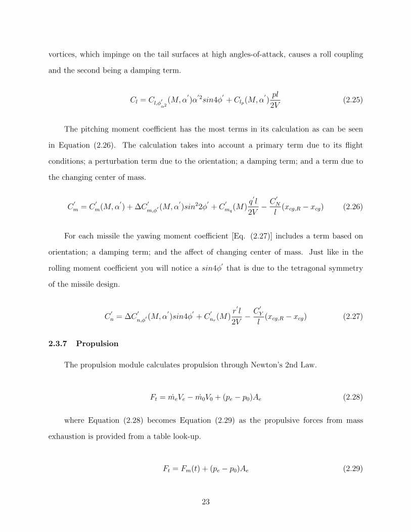
generation used in this research is shown in Figure 3.2 along with a more in depth look at

each core and its memory hierarchy.

27

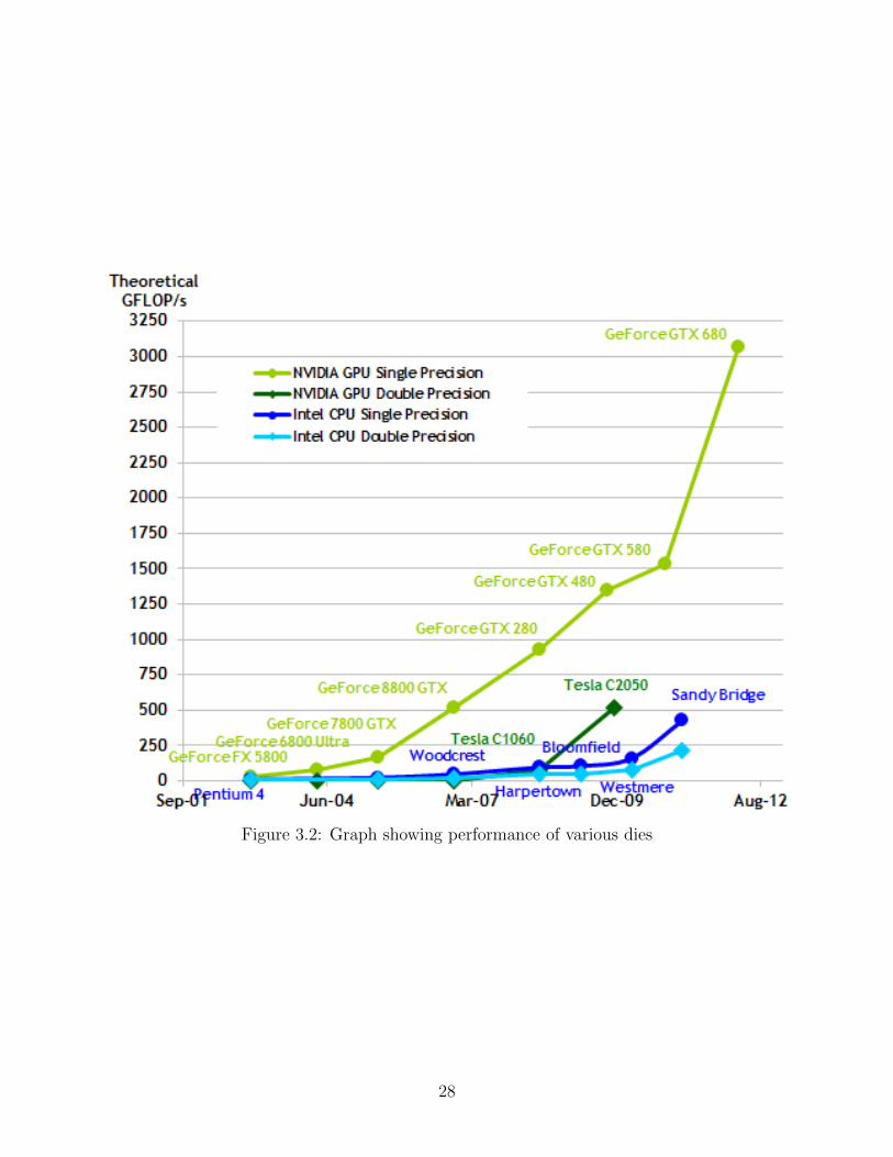
Figure 3.2: Graph showing performance of various dies

28

With all of these advantages there are pitfalls such as the clock frequency of the cards,

which tend to be about a third of the frequency current high end CPUs are clocked at.

We work around this by making sure we schedule enough missiles to be running at once.

The more data being processed (up to a point) at once the larger the performance increase.

Another pitfall, is the necessity of having to transfer data to and from the devices memory.

The less transfers there are during execution, the better the GPUs may be able to hide the

latency. Limited resources, as with any system, is another big concern. The device memory

on this particular card only has one gigabyte of storage which limits the number of vehicles

capable of being sent over to the device. Unlike the systems memory one cannot add memory

to the device. A new device with more memory built would need to be purchased for larger

projects. IEEE 754-2008 floating point standard for FERMI architecture

Figure 3.3: Core Comparison Table

29

3.1.1 Schedulers

The GigaThread Engine will schedule warps (32 threads) to each SM in a way that will

decrease run-time. The warp schedulers will then take over and schedule the execution of

each warp somewhat ”simultaneously”.

Figure 3.4: Streaming Multiprocessor

There are only 32 cores per SM, as can be seen in Figure 3.4 which means only 32

threads, or instructions, may be executed at any given time. However, the warp scheduler

schedules the execution of each warp in a way that each core rapidly computes instructions

for different warps - and thus threads - at any given time. An example of this scheduling

30

would be if warp 1 has a memory call and is waiting on the returned data then warp , lets

say, 7 which has its next instruction waiting, will be executed. This is Nvidias way of hiding

latency, by constantly cycling different warps. In our case, you can think of this as the

scheduler cycling through 32 different missiles at a time.

3.1.2 Memory Hierarchy

There are multiple levels of memory access integrated within the chip and outside the

chip, as seen in Figure 3.5. On the die resides thread specific cache, block specific shared

memory, and constant shared memory. These are the fastest memory locations as they reside

on the chip and require around 20 clock cycles to access necessary data.

Shared memory may be the most powerful tool for a developer to utilize to accelerate

calculations. If each core calls upon the same address within the constant or blocked shared

memory it is accessed once and broadcast across each core instead of individually accessing

the data independently. Also, compared to the global memory access times of around 200

cycles, it is intrinsically much faster.

The global memory resides on the card, but not on the chip. This is where the majority

of your data is stored. It is essentially RAM for the GPU.

3.1.3 New Architecture Versions

There are already new generation of cards available for CUDA computing code-named

Kepler and Maxwell. With these cards you can concurrently run multiple kernels (sub-

routines) from multiple CPUs on the same card, access global card memory from different

devices and share memory with the system, which alleviates the necessity of having to trans-

fer data to the card before executing the kernel. So, having multiple cards ultimately adds

performance and resources.

31

Figure 3.5: Memory hierarchy of CUDA Architecture

32

Chapter 4

CUDA Implementation

4.1 Design

The Six-DOF CUDA implementation was not a trivial process, as many hurdles had

to be overcome. Problems ranged from appropriate data management and table identifica-

tion, to issues with Windows Operating Systems’ Windows Display Driver Model (WDDM)

graphics cards safeguard, which prevent any lengthy use of such. The design of the im-

plementation was such that it would ease the burden of transferring data to-and-from the

GPU while keeping a comparatively similar simulation, and data structure to the original.

This design was mainly chosen to accurately compare serial vs. parallel code. This in turn,

showcases the the capability of the devices if proper parallel code were to be designed.

There are two noticeable additions to the serial code, when looking at the GPU flow

chart[Figure 2.6], or code: Packaging for the card and Send/Retrieve Data. Due to the

card not supporting arguments that have virtual components (polymorphism) it is necessary

to encapsulate the data in a supported structure and be sent to the card accordingly to

be operated on, as shared memory space is not supported for this particular architecture.

Meaning, data must be stored locally on the graphics card to access the data.

4.2 Missile Structure

The structure of missile objects is very intuitive for the original coding. One can see

how each missile has its own property tables, geometric variables, state variables, etc.; this

is not the case for the GPU Missile structure.

33

The original coding creates a list of missile objects each of which contain there respec-

tive, necessary data which defines how they will fly: Data Decks, which encapsulate tables

necessary for simulation (i.e. mass tables and aerodynamic tables) and vehicle variables

(e.g. mach, euler angles, transform matrices, etc.) which vary in type from int to matrices.

This combined with the intrinsic polymorphic design, provides an easy interface to call the

necessary functions to simulate each missile. However, as stated earlier, it is ill-suited for

the transfer and execution of the simulation on the card.

Figure 4.1: Dr. Zipfel Serial Vehicle List Implementation

34

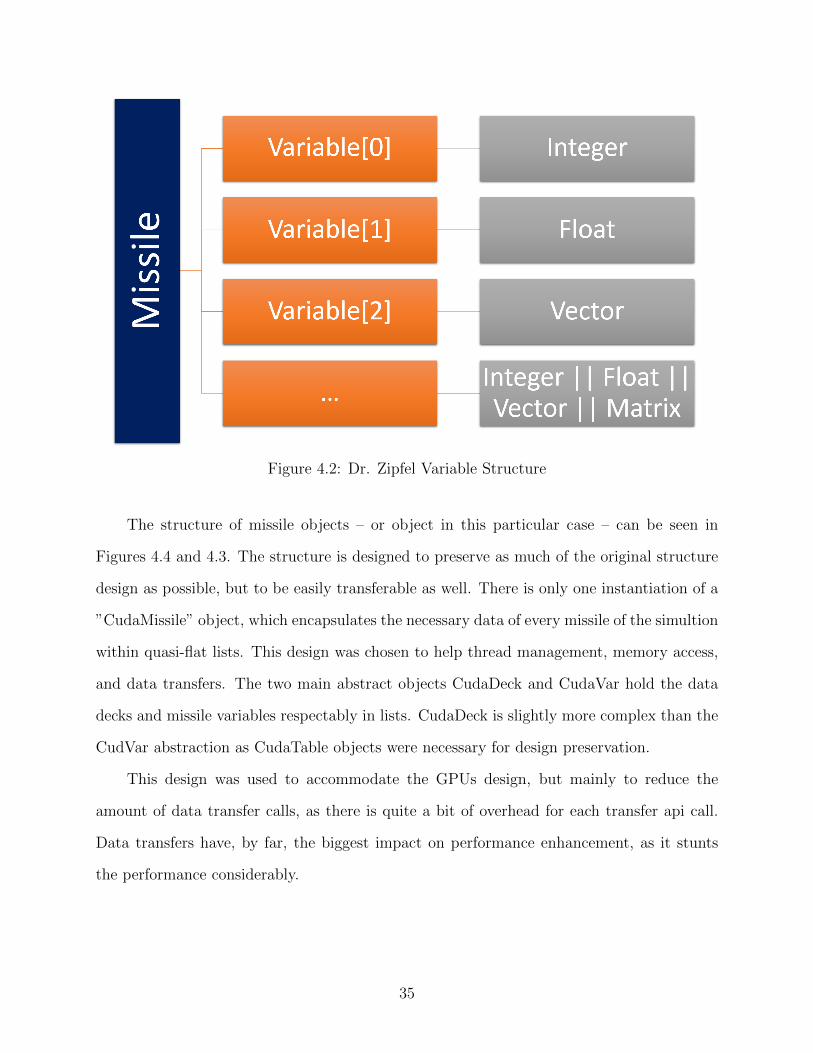
Figure 4.2: Dr. Zipfel Variable Structure

The structure of missile objects – or object in this particular case – can be seen in

Figures 4.4 and 4.3. The structure is designed to preserve as much of the original structure

design as possible, but to be easily transferable as well. There is only one instantiation of a

”CudaMissile” object, which encapsulates the necessary data of every missile of the simultion

within quasi-flat lists. This design was chosen to help thread management, memory access,

and data transfers. The two main abstract objects CudaDeck and CudaVar hold the data

decks and missile variables respectably in lists. CudaDeck is slightly more complex than the

CudVar abstraction as CudaTable objects were necessary for design preservation.

This design was used to accommodate the GPUs design, but mainly to reduce the

amount of data transfer calls, as there is quite a bit of overhead for each transfer api call.

Data transfers have, by far, the biggest impact on performance enhancement, as it stunts

the performance considerably.

35

4.3 Data Deck, Table, and Variable Structure

The packaging proved to be a more difficult task than anticipated since there are many

original levels of encapsulation for the vehicles data decks. As is the nature of encapsulation,

much of the table data is hidden below many levels of abstraction to make the design of the

software correlate to intuitive concepts. The data transfer CUDA runtime API call provided

by Nvidia, does not support a transfer of classes as a whole. The transfer function transfers

specified amounts of linear, flat memory, which is best for the GPU memory controller. This

becomes a problem when trying to send data to the card, as the necessary data is trapped

beneath layers of abstractions. To reduce the amount of memory transfer calls, each level of

abstraction and encapsulation was restructured to transfer necessary data all at once from

an array instead of individually transferring a single word for each transfer.

Dr. Zipfels Six-DOF uses the Standard Template Library’s (STL) string class for certain

control structures, and naming of data members. This is a convenience for CPU computing,

but is not supported in Nvidias GPUs. To overcome this barrier, an enumeration was applied

to each table, and data deck, for identification purposes. Many of the subroutines, which

used the string class, were re-written to accommodate the enumeration as well.

The card does not have the ability to write to system memory so, once the simulation

has executed completely, the necessary data blocks will be sent back to the host to be written

to appropriate files. This may seem to be a downfall, but will be more efficient than writing

each step per integration step.

Some utility functions were easier to convert than others, such as the provided matrix

class. A simple qualifier that flags the GPU compiler to create a version of the code for the

card, and a simple macro to insert host or device compatible code was all that was needed.

Optimization of the matrix class for device was not undertaken as it was not our goal, and

would have been proven to be futile.

The most difficult task was the memory management of all of the necessary missile

data for each simulated missile. The data structure used is very similar to the design of

36

Dr. Zipfels, but it is not polymorphic. The GPU data structures have a design which only

supports missiles but hold true to the original design as much as possible. This structure

was kept so a comparison between the CPU code and GPU code could be made under fair

circumstances. This data structure is not ideal for memory management on the card. So,

the presented results may seem very useful, but are far from optimal for the device.

Figure 4.3: CudaDeck Encapsulation

37

Figure 4.4: CudaVar Encapsulation

4.4 CUDA Simulation

The CUDA implementation of the simulation maintains the same execution flow as the

original with a few additions to accomodate the administration of data on the card. This was

a fairly simple port with a few tweaks for Windows WDDM, which prevented the simulation

from running with the original CUDA kernel design and data access.

To instantiate the simulation, a CUDA kernel must be invoked. The CUDA run-time

dictates that you must provide the number of threads per thread-block and number of thread-

blocks that should be scheduled to execute the kernel along with any parameters declared

in the prototype of the kernel. This variable number of threads is a tuneable feature. The

CUDA kernel will run differently for each different configuration, even if the number of

total threads running are identical. This particular trait of thread granularity was studied

to resolve the effect of the fongiuration parameters and to find the optimal configuration

of threads to run the simulation for multiple population sizes. The results of the different

configurations are presented along with the optimization metrics in the next chapter.

38

The structure of the kernel follows the same control flow as the original serial coding.

Each time the kernel is invoked, it executes the modules – as described in Chapter 2 – to

complete one iteration (or time step). This design is a secondary design. The decision to

change was made for multiple reasons: Windows WDDM, was the main motivation to alter

the original kernel; and poor design would be the secondary reason for a change.

The first kernel design was structured to run the entire simulation in one kernel call.

The execution was hindered by the Timeout Detection and Recovery feature, provided by

an version of windows beyond Windows Vista. Basically, the operating system watches the

graphics card for time-outs, and if it suspects such, it will attempt to reset the device. This

graphics card was not designed with intentions for heavy scientific computations; although

being capable, sending a task which requires an extended amount of time and resources to

complete, will undoubtedly cause the operating system to believe the card has stalled. If

the card were to be headless (void of any display connections), this may not be the case;

however, the firmware of the card may signal it is a piece of display hardware regardless and

trigger a stall. The solution to this road block was not documented very well at the time

of study. Fellow CUDA developers – with a small budget to a comparatively cheap CUDA

device for their study – were the biggest help. A more in depth discussion of the problem

WDDM presents, and the multiple solutions, is provided in Appendix A.

The nature of kernels drives them to be short in execution time, and schedule friendly.

Having the entire simulation execute in one kernel call is not schedule friendly and can take

up to several minutes to complete, depending on the kernel size, or missile population size

in this instance.

Due to the device being a separate processor, which uses private memory, the CPU has

no indication of whether the simulation has completed unless it has reached the max allotted

time. However, we do not need to run a simulation indefinitely if every missile has completed

its flight. To prevent a simulation running the max allotted time, a health-check routine was

implemented to check the status of the vehicles every so often. If the return values indicated

39

every missile had completed their respective trajectories, then the loop will be broken and

the simulation will resolve to the GA; otherwise, the simulation would continue.

40

Chapter 5

Results

5.1 Granularity Study

5.1.1 The Setup

The granularity test was carried out for multiple missile population sizes to see . The

maximum number of missiles which could be simulated for the CPU were 1440, due to a

memory leak within the original Six-DOF coding causing an overuse of system memory,

which Windows limits to 4GB. The GPU successfully tested all population sizes.

Different thread launch configurations (thread granularity) were used to test for optimal

simulation conditions ran on the GPU; each configuration was executed in high fidelity and

low fidelity mode, where the integration step was δt = .001 and δt = .01, respectively.

This amounts to 500 total granularity tests. Every missile in each test was geometrically

identical; however, the launch angle of each missile varied slightly. This was to ensure that

some missiles flew shorter times than others. This setup is not optimal for the card, as it

left some cores idle while others executed to finish integrating the remaining live missiles.

This could be thought of as a stress test for non-optimal case.

5.1.2 Results

Within these graphs one will notice some sections of plots are dashed, this indicates

our anticipated results. This was calculated by a linear extrapolation. Extrapolation was

necessary as there is a memory leak within the original Six-DOF coding, which caused the

simulation process within Windows to exceed its max allotted memory usage of 4GB. This

resulted in the inability to test the higher population sizes on the CPU. However, it was

41

possible to test all population sizes of 240, 480, 960, 1440, 2880, and 3840 successfully on the

GPU. Population sizes were chosen to activate each core within a Streaming Multi-Processor

on the card. The only size which does not activate each core is 240, as it is only half of the

number of cores which reside on the card.

5.1.3 Optimal Performance Trends

The following charts show the trend of performance for different population sizes, differ-

ent fidelity, and different precision. Figure 5.1 is a comparison of the different precision and

with the appropriate fidelity levels. A 1:1 performance is labeled as the black dashed line

meaning performance was equivalent; any value above the line represents a double precision

advantage where below is a single precision advantage. One will notice the higher the pop-

ulation size the more effective single precision becomes. This is expected as this particular

card has a higher throughput for single precision than it does for double precision. This can

be resolved from Figure 3.2.

42

Figure 5.1

5.1.4 Validation

Presented are two graphs which support the validity of the Six-DOF running on the

GPU. The coefficient of determination (R2) is shown in Figure 5.2. This uses a least squares

regression test. Truth data here is gathered from the original CPU simulation and compared

to the GPU results. Results are recorded to the 1E − 10 decimal for high fidelity assurance.

The results show a select few of any number of recordable simulation variables. All of the

presented variables show an R2 = 1, including the kinematic and attitude variables.

The next graph [Figure 5.3] shows the average error of recorded simulation variables

with respect to truth data. Most variables show little to no error with the exception of a

43

body rate. This can be explained by numerical boundary issues. Different compilers will

translate to different instructions for each die. As such, if domain issues such as 180 or -180

are encountered then each program has its own logic to decide which value it currently is.

If the CPU records a 180 and a GPU records -180, even if these number represent the same

angular position, the comparison still comes back negative.

These figures represent double precision data, as single precision data was widely skewed.

This discrepancy can be explained in a few different ways. As mentioned in [13] many CPU

compilers will use x87 instructions for single precision variables, which give them 80-bit

extended precision. There is no guaranteed way of disabling this feature and makes for

a difficult, unfair comparison between actual IEEE-754 32-bit single precision instructions

used on the GPU and 80-bit extended precision instructions used on the CPU. The GPU

also employs a Fused Multiply-Add operation which – as its name suggests – multiplies

and adds numeric values together when necessary, with only one required rounding step

resulting in better precision but different values. The act of parallelizing will sometimes

rearrange operations causing different numeric results as well.

44

Figure 5.2

Figure 5.3

45

5.1.5 Missile Design Study

5.1.6 The Setup

For each execution the GA was setup to vary each missiles tail semi-span, root chord,

trailing-edge sweeping angle, taper ratio, trailing-edge location, and launch angle. The

reported flight characteristics were apogee, ground range, burnout velocity, launch angle,

and flight time. Each characteristic weight was chosen so that each characteristic would

provide a relatively equal contribution. The weights used can be found in Table 5.1. The

GA was also instructed to test 200 different populations, each containing 240 missiles put in

a ballistic configuration. For CUDA execution,the granularity configuration of 6 threads and

40 thread blocks were used, as this configuration performed the best within the granularity

study.

Flight Path Characteristics Weights

Apogee: 0.50

Ground Range: 0.50

Burnout Velocity: 1.00

Launch Angle: 4.00

Flight Time: 8.00

Table 5.1: Flight path Characteristics Weights

The goal of the research was not to prove the GA could converge to a specific missile

design, rather it was to look at the convergence of the GPU and how it compares to the

convergence of the CPU. The weights for the flight path characteristics were assigned to

make each characteristic equally relevant as possible. There was not one characteristic

prefferred over another. Looking at the progressions of each missile parameter through the

200 different generations, you can easily come to a few different conclusions: some variables

have converged much more than others, the 200th population looks some what less converged

46

than population 100 for some variables, there are some wildly off average values for some

parameters which converge nicely, some variables converge to a range of values and a variable

does not converge at all.

The variables which converge to a well defined value tend to impact the simulation

the most with the slightest change in value providing a well defined answer for the given

weights. For the well behaved variables you will notice some values are skewed from the

averaged converged value. This is mostly likely due to the GA mutating duplicate missiles

as it was instructed to. Variables which converge to a range have an impact, but their effect

has little impact once convergence has reached this defined range. As one might be able to

see, the 200th generation appears somewhat less converged – for some variables – than they

were for the 100th generation. I believe this to be the GA trying to converge to a final design

causing multiple duplicates which forces it to mutate a larger set of missiles. The final thing

one may notice is the failure of the Tail trailing edge sweep angle to converge. This variable

seems to have the least effect on the missile force coefficients, as change has little to no effect

on missile performance.

Tables 5.2 and 5.3 show how the GA Converges onto very similar missile parameters

with very similar flight path characteristics for either processor. Table 5.4 shows a strong

correlation between the optimization and granularity study results, showing that the GPU

has ran the optimization for the missile design twice as fast.

47

Missile Parameter CPU GPU

Tail Semi-Span (calibers): 0.99±0.01 0.99±0.01

Tail Root Chord (calibers): 0.50±0.01 0.50±0.01

Tail Taper Ratio: 0.50±0.01 0.50±0.01

Tail Trailing Edge Sweep Angle (deg): 1.32±1 1.32±1

Tail Trailing Location (m): 1.05±0.01 1.05±0.01

Launch Angle (deg): 66.1±1 66.1±1

Table 5.2: Test Systems Setups

CPU GPU

Apogee(m): 385.59 385.59

Ground Range (m): 956.35 956.35

Burnout Velocity (m/s): 99.34 99.34

Launch Angle (deg): 66.20 66.20

Flight Time (s): 19.17 19.17

Table 5.3: Average Flight Path Characteristics

CPU GPU

GA Time(hr): 4.66 2.33

Performance Increase: 1x 2x

Table 5.4: GA Performance

48

Chapter 6

Conclusion

6.1 The Goal

We set out to accelerate missile design optimization by combining a three software pack-

ages: IMPROVE, a Binary Genetic Algorithm; Aero-Design, a missile property calculator;

and an open source Six-DOF enhanced with CUDA coding.

6.2 Overcoming Obstacles

Many roadblocks had to be overcome to successfully implement our solution: a redesign

of object abstraction and data management was carried out to provide capability for the

GPU and to preserve original design to make a fair comparison; Software limits were found

within Windows WDDM, as we were forced to redesign the CUDA Kernel, so as to not

cause a system failure; proper CUDA kernel design was an acquired skill from failed attempts;

lessons were learned about the importance of careful memory management, as we were unable

gather conclusive data on the limits of the acceleration; careful data analysis was executed to

correctly interpret what appeared to be wildly incorrect results for single precision; learned

the importance in choice of compilers, as a fair comparison of single precision is only possible

if a CPU compiler enforces true single 32-bit precision; careful thread management with

appropriately sized missile populations had to be well thought out; restructuring of the GA

was undertaken to parrallelize the execution of the objective function.

When designing experiments for CUDA one must take these concepts and lessons into

account, as a pure port of code will not show a perofrmance increase. CUDA has been

designed for high performance computing for problems that are ever increasing in difficulty.

49

6.3 Conclusion of Results

We were able to show accelerations with both studies. A 2.5 to 8x increase in perfor-

mance was achieved with a pure simulation and a 2x performance increase was achieved for

missile design optimizations for the smallest missile population design tested in the granu-

larity study. In contrast, both studies correalte fairly well and is safe to assume one would

achieve similar correlation in performance enhancements for larger population sizes.

Double precision values were validated to a high degree of precision of 1E − 10 with

errors which can be explained by compiler differences. Missile design successfully converged

to what can be described as a range of missile variants which are capable of achieving similar

performance.

The results provide a fairly impressive outcome for this proof, as much of the program

design is ill-fitted for this type of device: double precision is not highly supported on this tier

of CUDA capable card, object based transfers cause extended transfer times, single precision

adheres to IEEE 754 standards unlike most CPU compilers which employ 80-bit extended

precision, slower processor clock, less resources were available.

Presented results, show a niche of where the GPUs are most effective. As many of

the other referenced studies suggest, the larger the data-set, or required computations, the

more effective the device becomes. However, there are limits to everything.As we were

unable to compare results beyond a populaiton size of 1440, we are incapable of drawing any

conclusions on the limits of the device.

With this proof of concept we have decreased the run-time of current software with a

new, user-friendly, cost-effective, and efficient implementation. Hopefully, this will encourage

others - especially those within the simulation field - to adopt such techniques and accelerate

their own current processes to provide quicker results for the computationally intensive work,

as well as provide crucial information when it is needed, rather than when you can get it.

However, there are many ways to improve this implementation even as it stands.

50

6.4 Future Work

With the newer architectures the necessity to transfer data to and from the device has

vanished as support for shared system memory has been introduced. Other newly supported

features for CUDA devices have been developed such as, Concurrent kernel execution to run

multiple optimizations concurrently. Multiple simulation metrics provide a glimpse of how

much performance enhancement is possible. If one were to write code designed properly for

these newer processors, one may realize truly astonishing accelerations.

6.4.1 Optimizations

A full optimization was not taken into consideration, as we were seeking a simple ac-

celeration of the Six-DOF for a fair comparison, as well as a proof of concept. There are

many characteristics and features of the card which could decrease the run-time, but were

not used.

One feature that was not utilized is data streams. The GTX 570 card has a execution

engine and a copy engine scheduler. With this one would be able to set up the card to

execute a time step of the integration process (one run of the kernel) and copy the previous

results back to the host to be written to file all concurrently. This hides latency and would

provide all of the data for each time step of the simulation. The benefit here is, having the

capability of seeing the entire simulation for each missile. The disadvantage would be the

necessity for two pools of memory to be allocated for the ith-1 and the ith integration steps.

Taking advantage of the shared memory, which is located on the processing chip itself,

reduces memory access times from about 300 clock cycles to about 20 cycles. The only

disadvantages is the amount of shared memory each SM has for each thread block, and

finding an appropriate use for such memory.

Another viable option included is more of a software advantage than a hardware imple-

mentation. One could use page-locked system memory instead of just device memory. This

keeps the operating system (OS) from paging the memory to the hard drive, thus keeping the

51

addresses statically defined as they are when allocation is performed. This reduces memory

transfer calls, but reduces the host memory available for the OS, which may cause more

harm than good. If all of the system memory is page-locked, then you may render the OS

from using it for other processes. This may cause the system to crash.

Data management optimization’s would allow coalesced access patterns to reduce data

fetching. This feature may have the biggest impact on the run-time. If one were to restructure

many class based storage structures for necessary missile data, one could take advantage of

this type of data fetching. As calculations progress, data requests will occur for each core,

that is working on a particular vehicle. With the current implementation, a class-based

structure, the data is hidden in multiple levels within the actual vehicles; when data is

requested for the same variable by 32 different cores the data access will undoubtedly make

32 different queries to the memory for each core. If the data were contiguous, then a single

128-bit query would be able to retrieve 32 4-bit data values or 4 32-bit data values, and so

on.

As it stands, many of the vehicle modules (methods) instantiate variables which are

local in scope to the module. This causes each core to instantiate an x number of variables

in the local L1 and Shared (L2) memory spaces, which could be used for other variable

storage. If these instantiations were removed, then memory and time can be recovered to

proceed with the actual simulation.

Granularity is an important factor with these cards, as can been seen within the study.

This can make a dramatic difference in reduction of run-time, as the schedulers can dispatch

instructions for different threads more efficiently, rather than waiting on data to be retrieved.

Using a non-display Nvidia Device in Tesla Compute Cluster (TCC) mode has many

advantages:

• Eliminating timeouts due to TDR,

• Use of CUDA with Windows Remote Desktop,

52

• Using CUDA within processes running as Windows services,

• And reduces latency of kernel launches.

Tesla and Quadro branded cards both support this driver model, but tend to be more

expensive than Geforce cards, as the dies are larger with the intentions of being used in

workstations and High-Performance Computing (HPC) platforms. With this, if one would

use a card purely for computational science, rather than an image processor and computa-

tional means, then you would free up more resources and gain the capabilities of decreasing

run-time and broadening the scope of the job being tackled.

As the use of CUDA devices increases, so does the feedback from professionals wishing

to see specific features in the next generation of cards. Future architectures will use shared

memory between the host and the card itself, thus reducing the necessity of having to

transfer all of the data to the card for completion. More avenues will become available to

constantly raise-the-bar for performance metrics, as new innovations are implemented within

the architecture, and APIs, of these cards.

6.4.2 Moment of Inertia’s

The addition of different moment of inertia’s (MOI) is where the main focus of future

work lies, as of now. This will generalize the initial missile data and widen the scope of

profiles the GA will be capable of fitting.

As MOI’s are very computationally intensive, it may, or may not, be advantageous to

implement a routine using CUDA to calculate them for multiple missiles concurrently as

well.

6.4.3 Additional Vehicle Modules

With most missile setups - in the modern era - having more capabilities than basic

ballistic missiles, one must consider these attachments/features and their respective functions

53

within the simulation. Such packages may include a guidance systems, seekers, thrust vector

controls, actuators, etc. As missile systems become more complex, so must the simulation

at which they are modeled with.

6.4.4 Closing

In closing, exploring new, faster ways has always been the next step in improving sys-

tems, society, science, etc. and dates all the way back to the invention of the wheel. There

are plenty of questions to address; let’s answer them.

54

Bibliography

[1] Nvidia Corporation, “CUDA C Programming Guide,” Nvidia Corporation, October,2012.

[2] Nvidia Corporation, ”NVIDIAs Next Generation CUDATMCompute Architecture:FermiTM,” Nvidia Corporation, 2009.

[3] Nvidia Corporation, ”NVIDIA CUDA Getting Started Guide for Microsoft Win-dows”,Nvidia Corporation, February, 2014.

[4] Peter H. Zipfel, “Modeling and Simulation of Aerospace Vehicle Dynamics,” secondedition, American Institute of Aeronautics and Astronautics, Inc., 2007.

[5] Calisa Cole, “CUDA Spotlight: GPU Accelerated Air Traffic Management,”http://developer.nvidia.com/content/cuda-spotlight-gpu-accelerated-air-traffic-management, January 2012.

[6] Penny Crosman, “Bloomberg Uses GPUs to Speed Up Bond Pricing,” Wall Street &Technology, September 2009.

[7] Anthony Gregerson, “Implementing Fast MRI Gridding on GPUs via CUDA,” Septem-ber 2009.

[8] S. Stone and J. Haldar and S. Tsao and W. Hwu and B. Sutton and Z. Liang, “Accel-erating Advnaced MRI Reconstructions on GPUs,” Journal of Parallel and DistributedComputings, September 2008.

[9] Matsuoka and Satoshi and Yutaka Akiyama, “HPC-GPU: Large-Scale GPU AcceleratedWindows HPC Cluster and Its Application to Bioinformatics and structural Proteomics(and Climate/Environment),” Tokyo Inst. of Technology, September 2008.

[10] Julien C. Thibault and Inanc Senocak, ”CUDA Implementation of a Navier-StokesSolver on Multi-GPU Desktop Platforms for Incompressible Flows”,Boise State Univer-sity,January 2009

[11] Kendall Atkinson and Weimin Han, ”Elementary Numerical Analysis”, University ofIowa,3rd ed. 2004

[12] Andrew S. Tanenbaum, ”Structured Computer Organization”,Pearson Education,Inc.,5th ed. 2006

[13] NVIDIA Corporation, ”CUDA Toolkit Documentation”,2011-2015

55

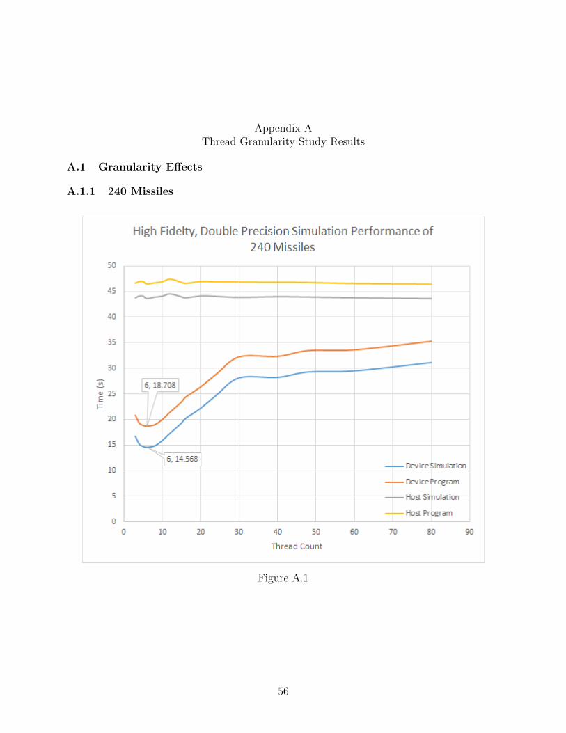
Appendix AThread Granularity Study Results

A.1 Granularity Effects

A.1.1 240 Missiles

Figure A.1

56

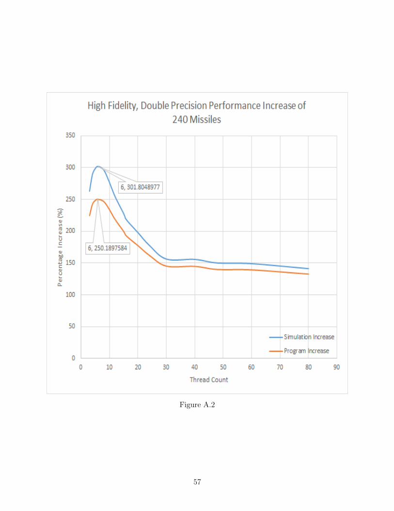
Figure A.2

57

Figure A.3

58

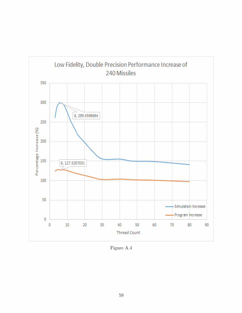
Figure A.4

59

Figure A.5

60

Figure A.6

61

Figure A.7

62

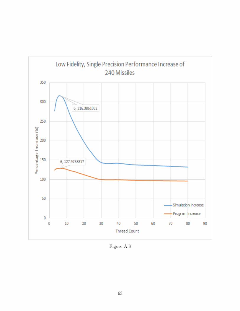
Figure A.8

63

A.1.2 480 Missiles

Figure A.9

64

Figure A.10

65

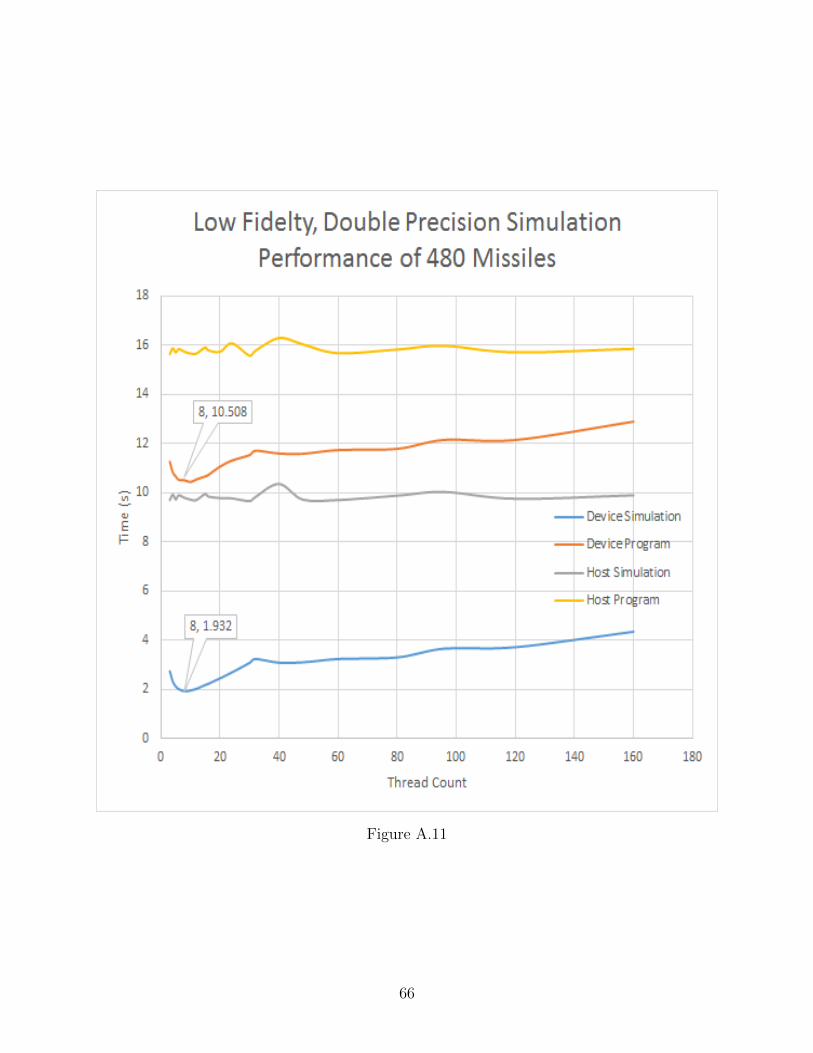
Figure A.11

66

Figure A.12

67

Figure A.13

68

Figure A.14

69

Figure A.15

70

Figure A.16

71

A.1.3 960 Missiles

Figure A.17

72

Figure A.18

73

Figure A.19

74

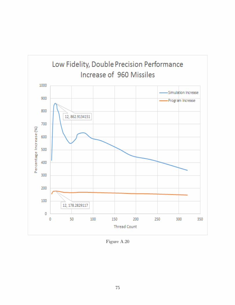
Figure A.20

75

Figure A.21

76

Figure A.22

77

Figure A.23

78

Figure A.24

79

A.1.4 1440 Missiles

Figure A.25

80

Figure A.26

81

Figure A.27

82

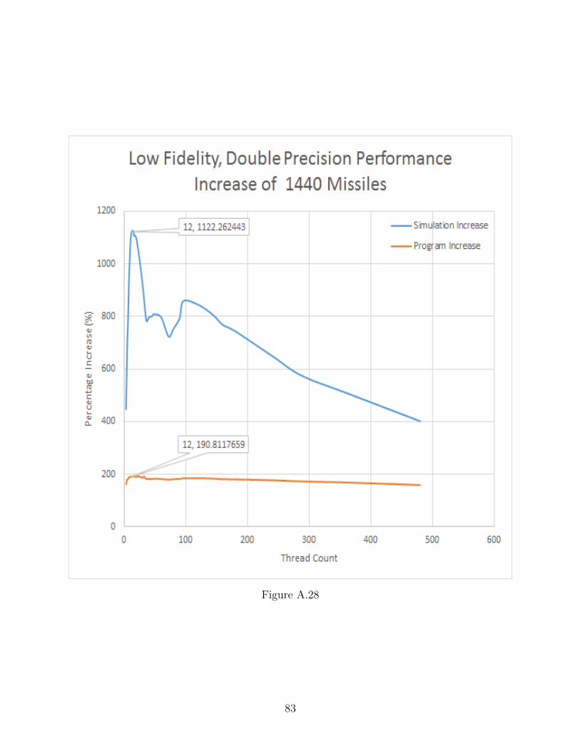
Figure A.28

83

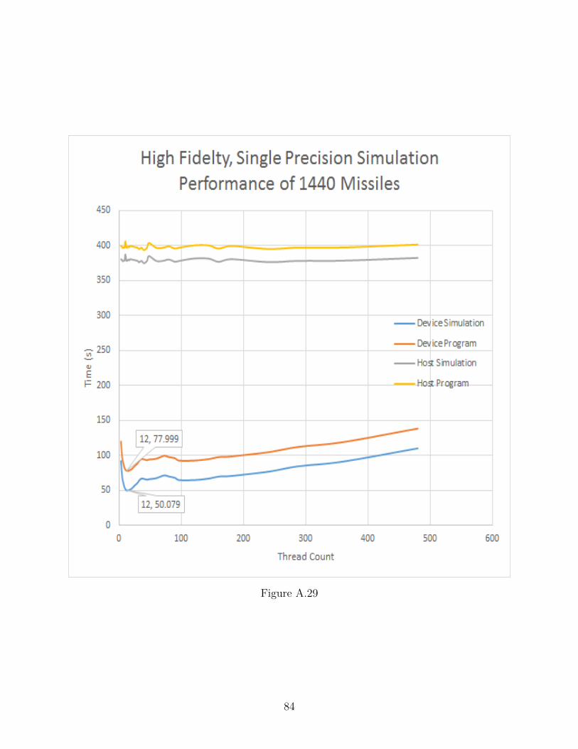
Figure A.29

84

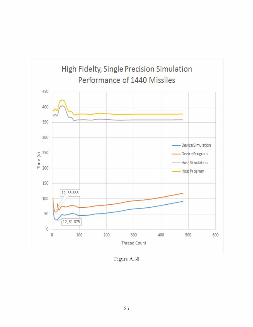
Figure A.30

85

Figure A.31

86

Figure A.32

87

A.2 Optimal Performance Trends

A.2.1 Double Precision

Figure A.33

88

Figure A.34

89

Figure A.35

90

Figure A.36

91

A.2.2 Single Precision

Figure A.37

92

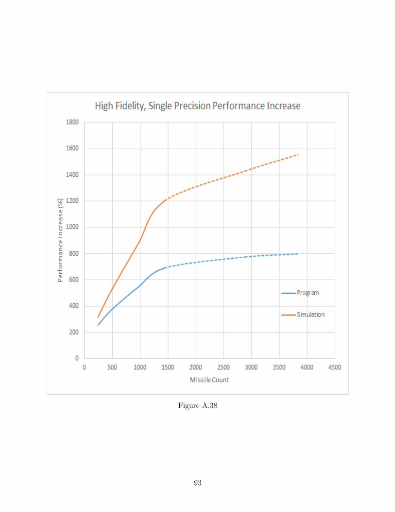
Figure A.38

93

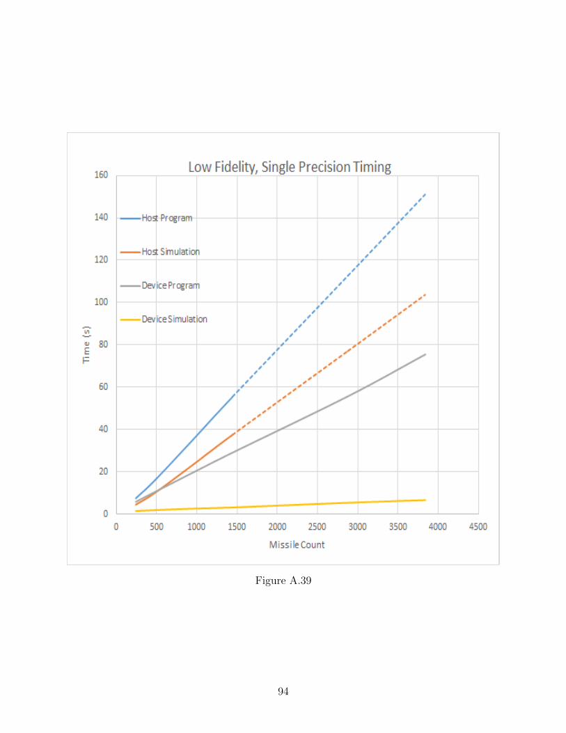
Figure A.39

94

Figure A.40

95

Appendix BOptimization Study Results

B.1 Results: CPU Convergence

Figure B.1: CPU Tail Semi-Span Values for Population 1


96


97

Figure B.4: CPU Launch Angle Values for Population 1



98

Figure B.7: CPU Tail Trailing-Edge Sweep Angle Values for Population 1



99

Figure B.10: CPU Tail Root Chord Values for Population 1



100

Figure B.13: CPU Tail Taper Ratio Values for Population 1



101

Figure B.16: CPU Tail Trailing-Edge Location Values for Population 1



102

B.2 Results: GPU Convergence

Figure B.19: GPU Tail Semi-Span Values for Population 1



103

Figure B.22: GPU Launch Angle Values for Population 1



104

Figure B.25: GPU Tail Trailing-Edge Sweep Angle Values for Population 1



105

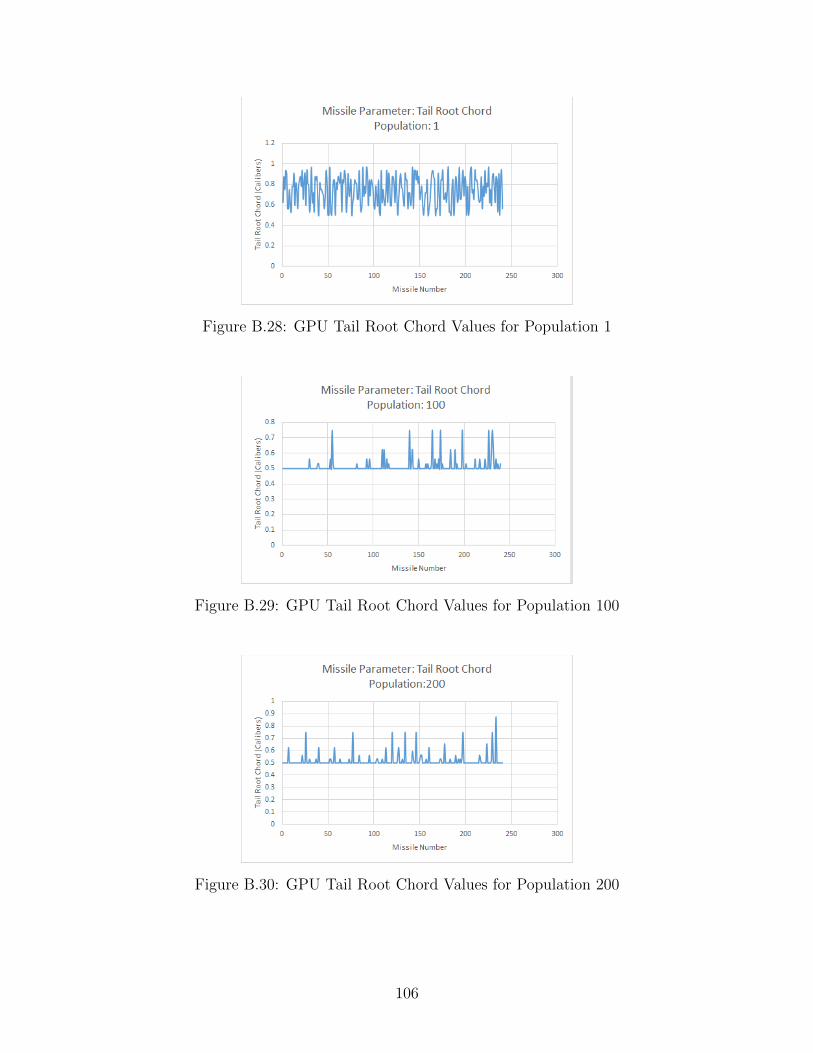
Figure B.28: GPU Tail Root Chord Values for Population 1



106

Figure B.31: GPU Tail Taper Ratio Values for Population 1



107

Figure B.34: GPU Tail Trailing-Edge Location Values for Population 1



108

Appendix CSetting up CUDA on Windows

C.1 Installing CUDA Toolkit

To develop CUDA code on Windows you must have at least:

1. Workstation with Windows

2. A CUDA Capable card

3. The very minimum, Microsoft Visual Studio 2010

4. And, CUDA Toolkit 5.5

CUDA Toolkit 5.5 is the minimum install recommended for this software. The target

cards has Architecture version of 2.0 meaning, any card that does not meet these require-

ments will not run this software, as it has been compiled for this architecture. The software

will run on any card that is 2.0 or higher.

The toolkit will plug-in to, and compile code, using Microsoft Visual Studio 2013 – if

one would rather do so, which is suggested. As these cards are made for graphics processing

by nature, you will have the option of debugging such code. To debug CUDA code – with

breakpoints and thread analysis – make sure you run the software in CUDA Debugging

mode.

A complete understanding can be obtained Nvidias programming guide [1], Fermi Ar-

chitecture White paper [2], and Nvidias getting started guide [3].

109

C.2 Windows Caveats

The Windows platform is, intrinsically, ill-suited for simulations as it has many built

safety measures implemented to ensure a smooth user friendly experience for the ”average”

desktop user. Windows Display Driver Model (WDDM) is one of these pre-cautions that will

limit, if not stall, the execution of software on any Nvidia Geforce branded cards. This is

due to the fact that these particular cards were not designed specifically for simulation, even

though their architecture is somewhat the same. Geforce cards are designed with CUDA

Architecture but intended for pure graphical processing. This makes these cards great for

development as they can be very cost efficient. Windows registers these devices, headless or

not, as such and applies the driver model to each card. Within the model is a registry value

called the Timeout Detection and Recovery (TDR) that determines how long the operating

system will wait on the card to refresh its output to the monitor if the operating system does

not receive a response in the set time span, then the model will reset the device to prevent

any undetermined behavior i.e. crashing, stalling, etc.

There are two different paths that can be taken to bypass this safety feature: manually

modifying the registry value or by using Nvidias control panel.

C.2.1 Manual TDR Override

To disable or delay TDR Manually:

1. Start up Windows Registry Edit

2. Navigate to "HKEY_LOCAL_MACHINE\System\CurrentControlSet\Control\GraphicsDrivers"

3. Add appropriate registry elements

(a) To delay TDR

i. Add a new DWORD named TdrDelay

110

ii. Tune the data value to your that fits your kernels run-time. (The value has

units of seconds.)

(b) To disable TDR:

i. Add a new DWORD named TdrLevel

ii. Change the data value to 0 (or 1 to enable)

4. Restart your system for your registry values to take effect.

C.2.2 Nvidia Nsight Monitor Option Override

To disable or delay TDR using the Nvidias Nsight Monitor:

1. Startup Nvidia Nsight either by navigating through the start menu or the Nsight Menu

in Visual Studio, seen in Figure C.1a

2. Once Nsight Monitor is running, go to your icon tray; right click Nsights icon, click

options

3. In the General section you should see Microsoft Display Driver with two fieldsas seen

in Figure C.1b:

(a) WDDM TDR Delay: This field changes the amount of time Windows waits to

hear back from the card before it restarts the card. You may be able to tune this

value depending on your kernel run-time.

(b) WDDM TDR enabled: This field enables or disables the display driver feature

entirely. It is best not to disable this feature, for if your kernel does take an

extended amount of time, you will not see a refreshed screen(i.e. your systems

will look frozen).

4. Restart your system as these fields modify your registry values.

111

(a) Start Menu Directory

(b) Options Menu

Figure C.1: Disabling/Delaying TDR Through Nsight

112

Appendix D

Six-DOF Versions

Included in the source coda for the CUDA implementation is a header file that contains

many flags that will trigger certain sections of code to be inserted for their respective reasons.

This gives the ability to compile different versions of the code to achieve different objectives.

Provided in the code below are all the necessary constants and flags used in the project.

The flags that provide different versions, and their respective sub-versions:

• MENU - Compiles the Six-DOF to print a command window menu which was included

for future user cases if one desired to implement different Six-DOF’s with different

modeling

• PRECISION - Flag will change the floating point type from double to single-precision

depending on its definition

• CUDA SDOF - Flag that defines whether the CUDA implementation or Dr. Zipfels

version is compiled

1. DEBUG - Flag will include debug software to debug CUDA implementation

(a) HTD - Debug flag for Host to Device Transfers

(b) DTH - Debug flag for Device to Host Transfers

(c) MATRIX - Debug flag for Matrix object transfers

(d) DATA - Debug flag for CudaData data structure transfers

(e) VAR - Debug flag for CudaVar data structure transfers

(f) TABLE - Debug flag for CudaTable data structure transfers

(g) DECK - Debug flag for CudaData data structure transfers

113

2. TEST

(a) USER - Defines code which would let a user choose which CUDA capable

device to use in execution

(b) INSTANCE - Defines code which calls an instance of the six-dof for better

memory management

(c) VALIDATE - Defines code which validates the GPU execution with the CPU

execution

i. VSTEP - Defines number of times the simulation will be validated

ii. ERR TOL - Defines the error tolerance of the validation

(d) TEST240 - Defines code which finds optimal kernel launch parameters for

device

(e) WIN32 DCOM - Flag to collect system properties

• VERIFY - Debug flag for verifying/validating device six-dof execution

114

Appendix E

Help Documents

Included in the software package are many different routines which have been separated

from the main routine to give more freedom to the user, and to aid in the research process.

The routines include:

• AERODSN Standalone.exe

• CUDASDOF DP/SP.exe

• SimulatorSetup.exe

• TestGenerator.exe

• Validator.exe

• WriteADInput.exe

• WriteZipfelInput.exe

• ZipfelSDOF DP/SP.exe

Also included are, some batch files which will run certain routines with file name ap-

propriate command line arguments, the source code for each routine and the debug files for

each routine to use if one were to run into any problems.

115

E.1 Six-DOF’s

This section will help with the correct execution of the simulation routines. Research

was carried out on both Double Precision(DP) and Single Precision(SP) performance. As

such, there are four different versions of the simulation software; two different precision

executable’s for two different simulation versions which execute on their respective cores (i.e.

CPU, GPU).

E.1.1 ZipfelSDOF DP/SP

Description:

The ”Host” version of the simulation does not take any command line arguments

to carry out the simulation of the missile line-up within the input file. However,

the inputs relative file location is hard coded within the executable. This requires

that the Software package directory structure must remain the same for correct ex-

ecution. If one had the desire to hand edit the input file, one may navigate to

..\Input Files\ZInput.dat to do so.

Example:

[Executable]

ZipfelSDOF DP.exe

Command Line Arguments:

None

Input Files:

• ”Zinput.dat”

Output Files:

• Temporary Timing File (*.dat)

• Validation File (*.val)1

1When triggered in input file

116

E.1.2 CUDASDOF DP/SP

Description:

CUDASDOF DP/SP.exe takes two command line arguments each being a kernel

launch parameter. Assuming one is in the correct directory or using a batch file, the

correct command line can be seen in the following example.

The simulation will launch and execute in the same manner as ZipfelSDOF*.exe

would. The only difference being that the execution will be carried out on the GPU

rather than the CPU.

If no command line arguments are given then the default setup is 4 threads with

60 thread blocks as launch parameters for the CUDA kernel.As such, the default

input file should have only 240 missiles to simulate. If not, the executable will behave

unpredictably

Example:

[Executable] [Thread Count] [Thread Block Count]

CUDASDOF DP.exe 4 60

. This example will launch a CUDA simulation which is design to simulate 240

missiles as the launch parameters designate so.


• Thread count kernel launch parameter

• Thread Block count kernel launch parameter

Input Files:

• ”Zinput.dat”

117

Output Files:

• Temporary Timing File (*.dat)

• Validation File (*.val)2

2When triggered in input file

118

E.2 SimulatorSetup

Description:

The SimulatorSetup can be thought of as a Simulator Administrator. There are

four different Test modes; 4 different missile count modes; two different file open

modes; two different precision modes; two different validation modes and the option

to provide the integration step for each test.

Example:

[Executable] [File Open Mode] [Test Mode] [Missile Count] [Integration Step]

[Precision Mode: String] [Validation Mode]

SimulatorSetup.exe 1 2 2 .001 Double 1

This example will launch a setup where every data file is wiped clean; Run a

granularity test; write a setup for 960 missiles; launch the Double precision version of

each simulator; integrate the simulation with a time step of .001 seconds; and validate

the simulation.


• File Open Mode

� 1 - Clean Mode: Will erase the content of any file which is opened

� 2 - Append Mode: Will append any data at the end of each opened file

• Test Mode

� 0 - Host Test: Will run Host Test (CPU:Zipfel*.exe)

� 1 - Device Test: Will run Device Test (GPU:CUDASDOF*.exe)

� 2 - Granularity Test: Will run a Test which will vary the parameters of the

CUDA Kernel to Collect data on each different configuration

119

� 3 - Ultimate Test: This test will run granularity tests on every missile con-

figuration; both precision versions; and with two different integration step

sizes

• Missile Count

� 0 - 240

� 1 - 480

� 2 - 960

� 3 - 1440

� 4 - 2880*

� 5 - 3840*

• Integration Step - The integration step is a floating point input which is chosen

by the user. However, due the discretization of time in a simulation, you will need

to choose an appropriate step size, or the simulation will fail as it will become

unstable.

• Precision Mode

� ”Double” - Setup will launch the Double precision version of each simulator

� ”Single” - Setup will launch the Single precision version of each simulator

• Validate Mode

� 0 - Setup will not validate the simulation

� 1 - Setup will validate the simulation

* = will only run in Device Test Mode

120

Input Files:

None

Output Files:

None

121

E.3 TestGenerator

Description:

TestGenerator will read-in the number of missiles; the integration step size; and

the validation flag. Once read in, Aero-Design will be invoked to calculate force

coefficients; WriteDataDeck will be invoked to write the data decks to the appropriate

format for the simulators to read; and WriteZipfelInput will be called to write the

appropriately formatted input file for the simulators

Example:

[Executable]

TestGenerator.exe


None

Input Files:

• ”TestGeneratorInput.dat”

Output Files:

None

122

E.4 Validator

Description:

To validate one must have record of simulation for each simulator (i.e. Device

record and Host record). The Host record serves as a model for the Device to be

modeled against. The validation routine will find the coefficient of determination

(R2) of the Device record for the selected variables in ”..\Output Files\Validation

Files\ValidateList.dat”. The R2 value and average error of each variable is written

to two separate files respectively. Paths to each file have been hard coded into the

routine so directory structure must be maintained to operate correctly.

Example:

[Executable] [Model File Name] [Test File Name] [Validation File Name]

[Precision Mode: String] [Open Mode]

Validator.exe Missile240 220.val Missile240 220.val Trial Double app


• Model File Name (*val)

• Test File Name

• Validation Files Name

• Precision Mode in ”string” Format

– Double: Will force the file to be appropriately named for Double Precision

– Single: Will force the file to be appropriately named for Single Precision

• File Open Mode

– app: Will force the appending of data to a file if already exists

– trunc: Will force the opening of an existing file to be cleared of contents

123

Input Files:

• Model File Name (*.val)

• Test File Name (*.val)

Output Files:

• Validation File Name.dat

• Validation File Name.csv

124

E.5 Write Routines

The write routines provided are supplementary functions which were written in C++

to have better control over the file format. Each will write necessary files for the proceeding

step in the simulation process.

E.5.1 WriteZipfelInput

Description:

This executable will write the ”ZInput.dat” file which is used as the simulation

input file. The data read in is the generation number to appropriately name the sim-

ulation; Missile count to correctly define the simulation; validation mode to correctly

write the validation option into the file; and ”ZSetup.dat” which provides the launch

angle of each missile.

Example:

[Executable] [Missile Count] [Generation Number] [Validation Mode]

WriteZipfelInput.exe 240 1 1

This example will know to write in 240 missiles; appropriately name the simulation

Generation 1; and write the validation option to output validation metrics.


• Missile Count

• Missile Generation

• Validation Flag

� 0 - Will not trigger the writing of the validation flag to the simulation input

file

� 1 - Will trigger the writing Validation flag to Simulation input file

125

Input Files:

• ”Zsetup.dat”

Output Files:

• ”ZInput.dat”

E.5.2 WriteDataDeck

Description:

This executable will read in the force coefficients – calculated by Aero-Design

– from ”ADResults.dat” and write the Aerodynamics deck needed for simulation

execution.

Example:

[Executable] [Missile Number]

WriteDataDeck.exe 240

This example will write missile number 240’s Aero deck file(i.e. Aero Deck240.asc).


• Missile Number

Input Files:

• ”ADResults.dat”

Output Files:

• Aero Deck File (*.asc)

126

Accelerating Binary Genetic Algorithm Driven Missile ... · A.15 Low Fidelity, Single Precision...

Documents

Transcript of Accelerating Binary Genetic Algorithm Driven Missile ... · A.15 Low Fidelity, Single Precision...