Clemson UniversityTigerPrints

All Theses Theses

8-2008

Accelerated Life Testing of Electronic RevenueMetersVenkata ChaluvadiClemson University, cvnharish@gmail.com

Follow this and additional works at: https://tigerprints.clemson.edu/all_theses

Part of the Electrical and Computer Engineering Commons

This Thesis is brought to you for free and open access by the Theses at TigerPrints. It has been accepted for inclusion in All Theses by an authorizedadministrator of TigerPrints. For more information, please contact kokeefe@clemson.edu.

Recommended CitationChaluvadi, Venkata, "Accelerated Life Testing of Electronic Revenue Meters" (2008). All Theses. 470.https://tigerprints.clemson.edu/all_theses/470

ACCELERATED LIFE TESTING OF ELECTRONIC REVENUE METERS

A Thesis

Presented to

the Graduate School of

Clemson University

In Partial Fulfillment

of the Requirements for the Degree

Master of Science

Electrical Engineering

by

Venkata Naga Harish Chaluvadi

December 2008

Accepted by:

Dr. E. Randolph Collins, Committee Chair

Dr. Elham B. Makram

Dr. Michael Bridgwood

ii

ABSTRACT

Electricity meters are devices that continuously record electrical energy

consumption. In the past, meters have been of electromechanical type and consisted

windings and moving parts. Electromechanical meters tend to be bulky, less accurate and

more susceptible to tampering. As with other aging power system infrastructure in the

US, most electricity meters are around 40 years old and are nearing the end of their

intended lifespan. Concerns over the accuracy of these electromechanical meters along

with advances in technology have led to development of new electronic meters which

have additional benefits such as light weight, tamper-proof mechanisms, harmonic

detection and Advanced Metering Infrastructure (AMI) features. Utilities intend to spend

millions of dollars over the next few years in replacing these aging electromechanical

meters; however the new meters contain electronic parts that are typically more sensitive

to environmental conditions and abnormal voltage conditions. The drive to replace older

meters will not meet the expectations, either in terms of functionality or expected profits,

if the new meters drift in accuracy or fail relatively quickly with respect to their

electromechanical counterparts.

This thesis discusses the methods and techniques used in industry to perform

reliability and accelerated life testing analysis and such a study is performed on electronic

meters to predict their life. Industry standards are reviewed and accelerated test plans are

developed to systematically study the effect of environmental stresses on electronic

revenue meters by using failure time distributions, degradation parameters and

iii

accelerating factors to predict their life. A Human Machine Interface (HMI) was

developed in LabVIEW to interface the data acquisition devices with software, and thus

facilitate continuous monitoring of environmental parameters and the health of test

specimens placed inside an environmental chamber. The HMI also has the capability of

generating automated periodic reports and emails for review by management.

Since the lab test data from accelerated life testing of electronic meters was yet to

be obtained, the statistical analysis procedure, derived from the literature review, was

demonstrated using ALT data from other electrical and electronic components. ALT data

for cable insulation was obtained from the literature, and the failure data analysis to

predict the relation between cable life and temperature was demonstrated. Another

example illustrating degradation analysis using degradation data of LEDs, using current

as an accelerating stress, was provided. Finally, the causes for lack of data were analyzed

and improvements in testing procedure were recommended.

iv

ACKNOWLEDGMENTS

I would like to sincerely thank Dr. E. Randolph Collins for his guidance,

motivation and patience throughout my Masters program. Without his support, none of

this would have been possible. I would like to thank Dr. Elham B. Makram and Dr.

Michael Bridgwood for their support as instructors and for serving on my committee.

I thank Mr. Charles Perry of Electric Power Research Institute (EPRI) for

providing this project topic and research grant for the support of my thesis and the PQIA

lab.

I would also like to thank Curtiss Fox and Daniel Fain for their advice and

assistance in the lab.

Finally I would like to thank my parents whose continuous love and

encouragement have got me through stressful times.

v

TABLE OF CONTENTS

Page

TITLE PAGE....................................................................................................................i

ABSTRACT.....................................................................................................................ii

ACKNOWLEDGMENTS ..............................................................................................iv

LIST OF TABLES.........................................................................................................vii

LIST OF FIGURES ......................................................................................................viii

CHAPTER

1. INTRODUCTION .........................................................................................1

2. OVERVIEW OF METERING TECHNOLOGY ..........................................6

Introduction..............................................................................................6

Electromechanical meters ........................................................................6

Electronic meters ...................................................................................11

Advanced Metering Infrastructure.........................................................15

Meter testing and calibration .................................................................17

3. RELIABILITY AND ACCELERATED LIFE TESTING..........................20

Introduction............................................................................................20

Data types...............................................................................................23

Statistical analysis..................................................................................25

Test plans ...............................................................................................42

4. DATA ACQUISITION SYSTEM...............................................................43

Introduction ...........................................................................................43

Data Acquisition system ........................................................................46

Energy and power measurement............................................................47

Temperature measurement.....................................................................59

Prototype ................................................................................................64

Original system at EPRI.........................................................................67

Human Machine Interface......................................................................71

vi

Table of contents (continued)

5. TEST PLAN, RESULTS AND DISCUSSION...........................................83

Test procedure........................................................................................83

Test results and discussion.....................................................................85

Recommended test plan .........................................................................87

6. ANALYSIS USING EXAMPLES ..............................................................89

Introduction............................................................................................89

Failure data analysis...............................................................................90

Degradation analysis............................................................................100

7. CONCLUSION..........................................................................................104

Future work..........................................................................................107

APPENDICES .............................................................................................................109

A: NI SCB 68 breakout board pin diagram ....................................................110

B: Type T thermocouple coefficients .............................................................111

C: LabVIEW program ....................................................................................112

REFERENCES ............................................................................................................117

vii

LIST OF TABLES

Table Page

3.1 Failure mechanisms and related stresses......................................................23

4.1 Acquisition devices used for the project ......................................................47

4.2 List of thermocouple types with characteristics...........................................61

6.1 Failure data of insulation specimens............................................................91

6.2 Anderson Darling test statistic values..........................................................97

6.3 Degradation data of LEDs .........................................................................101

viii

LIST OF FIGURES

Figure Page

2.1 Front view of an electromechanical watt-hour meter ....................................7

2.2 Components of a single-phase induction

watt-hour meter ........................................................................................8

2.3 Vector diagram of the operating quantities in a

watt-hour meter ........................................................................................9

2.4 Front view of an electronic watt-hour meter................................................12

2.5 Schematic of an electronic watt-hour meter ............................................... 14

2.6 Internal components of an electronic watt-hour meter ................................14

2.7 Schematic of an electronic watt-hour meter with AMR ..............................16

2.8 UTEC 5600 Universal Calibration device ...................................................18

2.9 Sample Utility meter calibration report .......................................................19

3.1 Effect of λ on the pdf of an exponential distribution...................................26

3.2 Effect of λ on the cdf of an exponential distribution ...................................27

3.3 Effect of β on the pdf of a Weibull distribution...........................................28

3.4 Effect of η on the pdf of a Weibull distribution ..........................................28

3.5 Effect of η and β on the cdf of a weibull distribution .................................29

3.6 Effect of σ on the pdf of a lognormal distribution.......................................30

3.7 Effect of µ on the pdf of a lognormal distribution.......................................30

3.8 Effect of σ on the cdf of a lognormal distribution .......................................31

ix

List of figures (continued)

Figure Page

3.9 Illustration of ecdf compared to a normal cdf..............................................35

3.10 Schematic of temperature cycle profile .......................................................40

4.1 Electronic watthour meter............................................................................48

4.2 IR pulses emitted by meters with different Kh constants ............................49

4.3 Pulse detection circuit ..................................................................................49

4.4 Schematic of software/hardware interface...................................................51

4.5 Flowchart of energy calculation algorithm................................................. 53

4.6 Relative sensitivity vs wavelength...............................................................55

4.7 Relative sensitivity vs viewing angle...........................................................56

4.8 Illustration of flexible gooseneck ................................................................57

4.9 Effect of slow sampling rate ....................................................................... 58

4.10 Thermocouple illustration............................................................................60

4.11 Thermocouple output contaminated with noise...........................................63

4.12 Schematic of the test setup.......................................................................... 65

4.13 Experimental set-up showing the resistor bank, meters

and transformer .................................................................................... 66

4.14 The entire prototype.....................................................................................66

4.15 Envirotronics Chamber at EPRI facility ......................................................68

4.16 Schematic of the experiment....................................................................... 69

x

List of figures (continued)

Figure Page

4.17 The actual test set-up at EPRI..................................................................... 70

4.18 Illustration of front panel and block diagram

in LabVIEW...........................................................................................73

4.19 Dialog box for manufacturer’s details .........................................................74

4.20 Main page of the DAQ software..................................................................76

4.21 Meter page of the DAQ software.................................................................80

4.22 Temperature page of the DAQ software......................................................81

5.1 Calibration results for high temperature tests ..............................................85

6.1 Flowchart of statistical analysis for accelerated life tests........................... 92

6.2 Histogram of the failure data at 110 °C .......................................................93

6.3 Histogram of the failure data at 130 °C .......................................................94

6.4 Probability plots of the failure data at 110 °C .............................................96

6.5 Probability plots of the failure data at 130 °C ............................................ 96

6.6 Lognormal characteristics of the failure data at 110 °C ..............................98

6.7 Lognormal characteristics of the failure data at 110 °C ..............................98

6.8 Arrhenius plot for cable insulation ..............................................................99

6.9 Degradation data ........................................................................................102

6.10 Inverse power law plot showing stress vs life ...........................................103

1

CHAPTER 1

INTRODUCTION

Electricity metering is a vital part of a utility’s distribution system since it is the

source through which the utility gauges a consumer’s utilization, and generates a monthly

bill, which is the source of revenue for itself. It is important for the meters to be as

accurate as possible because even the slightest under-reading of each meter can cost the

utility millions, as the meters are deployed on a large-scale. On the contrary over-reading

can also have an adverse effect since it could lead to legal issues and harm the reputation

of a utility. Meters of different types and complexities have been used since the 1900s

when electricity began to be produced and distributed commercially [1]. Most such

meters in the past were of electromechanical type and consisted of windings that

produced magnetic fluxes proportional to the current and voltage. These windings were

aligned to rotate an aluminum disk, which in turn rotates registers for display. They

worked on the working principle of an induction motor and sometimes are also called

induction disk watt-hour meters.

With the advent of electronics, electricity meter manufacturers started to

incorporate them into metering technology. The first fully electronic meters were

available in 1990s but were not deployed on a large scale because they were expensive

and many previously installed electromechanical meters were still within their projected

lifespan. In general, utilities did not replace a meter unless it was damaged. As a result,

2

most electricity meters have performed for around 40 years and are now nearing the end

of their lives.

Another reason for replacing old electromechanical meters has come with the

passage of the United States Energy Policy Act of 2005 [2]. By the guidelines in this

energy law, utilities are now encouraged to invest more resources into research pertaining

to renewable energy and energy efficiency. With restrictions on construction of new

thermal and nuclear plants due to environmental impact and the fact that hydro electricity

is almost 100% utilized, energy efficiency has become the primary objective of the 21st

century. A key feature for the success of this drive is demand response and real-time

pricing. Demand response refers to load shedding or reduction of consumption of

electricity (e.g. lighting, air conditioning, etc.) by the utility, with the approval of the

consumer, in order save costs by keeping expensive generators offline and continue

maintaining grid stability during peak demand hours. For this objective to be realized,

Advanced Metering Infrastructure (AMI) needs to be in place. These meters are capable

of two-way communication, remote disconnection, and real-time pricing, as well as other

features.

Due to the reasons mentioned in the paragraphs above, utilities intend to spend

millions of dollars in replacing the aging metering infrastructure over the next couple of

years. However, with electronic meters, reliability of electronic components is a concern

since they are particularly vulnerable to stresses caused by environmental conditions,

voltage, current, etc.

3

Reliability is defined as the ability of a product to perform as designed for the

expected lifespan under stated operating conditions. Reliability engineering deals with

application of engineering principles and techniques to evaluate the reliability of a

product and find potential areas for reliability improvement by identifying the most likely

failures and then identify appropriate actions to mitigate the effects of those failures.

Reliability engineering deals with the study of failure data which includes times to failure

and causes of failure. This data is acquired over the years from field-testing and products

returned under warranty, and in today’s competitive world it is not profitable to wait for

the accumulation of data from the field. Moreover, technology improvements are

occurring at such a rapid pace that failures in products in the field may not occur in the

new products for which the reliability needs to be predicted. In order to maintain the

competitive edge, engineers need to obtain failure data quickly, and for this purpose,

Accelerated Life Tests (ALT) were devised. In ALT tests, specimens of the actual

product are subjected to elevated stresses such as temperature, humidity, voltage, etc.

making them fail or degrade quickly. Stress levels should be chosen such that they would

lie in the elevated stress zone and not lie within destruct limits in which the device would

definitely sustain damage, thus providing no useful information. With data analysis, the

inferences can be extrapolated to normal usage conditions. The underlying assumption of

such tests is that the failure mechanism remains the same at both normal and elevated

stress conditions. Reliability studies and Accelerated Life Tests have been around since

1970s, and their use was initially limited to defense and military equipment. Over the

years, many manufacturers have developed reliability programs to improve the quality of

4

consumer products, achieve customer satisfaction, and reduce warranty costs. Many

classified documents from military ALT testing have been declassified and available,

along with other good resources of information on this subject [3, 4, 5].

Some of the failures that could occur in electronic systems can be attributed to

evaporation of electrolyte in capacitors, solder crack formation on circuit boards,

delamination of ceramic components, electromigration, and damage to microelectronic

devices, etc. Although in terms of reliability, electronics have improved tremendously

over the years and electronic meter manufacturers have strong reliability programs, a

third party verification was requested by several utilities to gain a higher level of

confidence before investing large amounts of money in replacing aging meters. As a

result, this thesis was partly funded by EPRI, which is in turn was funded by electric

utilities, to perform a research study to assess the accuracy and life of an electronic meter

in the field by utilizing accelerated life tests.

As the first phase of the project contract, an estimate of life of electronic meters in

the field is required with impact of environmental conditions. Other stresses such as

voltage and humidity will follow in later phases. Accelerated testing is performed on

electronic meters by subjecting them to high temperatures for extended periods in an

environmental chamber at an EPRI facility. The first step in assessing product life is to

obtain time-to-failures. From this data, the average life of the product and other

inferences can be made. Since it is not possible to observe the meters in the chamber

during operation, a Data Acquisition System was built to continuously monitor the health

of the meters. The fact that electronic meters have a built-in infrared LED for calibration

5

purposes has been exploited. Although the purpose of this LED is periodic calibration

either in the lab or the field, it has been used in this project to continuously monitor the

meters placed in the inaccessible environmental chamber. The software interface was

programmed in LabVIEW and the system was used to count the pulse output of an

electronic meter and calculate energy. When compared to a reference, the absence of

pulses or drift in recorded energy, beyond a threshold, was considered a failure. The

temperature of the chamber was also closely monitored with the system, since the control

system of the environmental chamber may be inaccurate or distant from the meter

location in the chamber. The system developed is flexible and can be adopted to be used

in any future testing operations with other stresses.

6

CHAPTER 2

OVERVIEW OF METERING TECHNOLOGY

Introduction

Revenue metering refers to monitoring the usage of a resource such as electricity,

water or natural gas for the purpose of generating revenue. Electricity is one of the more

important revenue generating resources and monitoring it can be more complicated than

others. This chapter discusses the fundamental principles of electricity metering and the

latest trends in this area, and is important since it compares and contrasts traditional

methods and new electronic meters. It also gives insight into the functionality,

construction, and calibration of these new electronic meters, which can be useful later

chapters.

Electromechanical meters

Traditionally electricity has been measured by the use of electromechanical

meters. Such meters have a proven track record of lasting over 40 years in the field, and

are not prone to catastrophic failures. Although they have other problems associated with

them, they generally perform reliably requiring only a calibration check once every 5-7

years. An electromechanical meter works on the principle of operation of an induction

motor. It contains a rotating aluminum disk in which the angular speed of this disk is

proportional to the voltage applied and the current flowing through the windings that

produce magnetic flux. Since it is based on this principle, the power factor is

7

automatically accounted for and the disk spins at a rate proportional to the true power (S).

The disk is then attached to a register through an appropriate gearing ratio, to obtain the

actual kilowatt hours seen by the meter.

Figure 2.1 Front view of an electromechanical watt-hour meter

(Source: www.tdsurplus.com)

Since the meter is based on the principles of an induction motor, the disk behaves

like a squirrel cage rotor where torque is produced by the induced eddy currents due to

the disk’s position in the time-varying magnetic field. The EMF is created by the current

carrying coils in conjunction with the voltage coils. In order to ensure that the

measurement is accurate, the torque (and hence the speed) should be at the maximum

8

possible value when the system is at unity power factor. To ensure this, a lag coil is used

on the voltage pole so that the current in the voltage coil lags the voltage by 90°. Current

in the lag coil, and hence the angle between voltage and current, can be varied using the

lag resistor. This is shown in the Figure 2.2. The permanent magnets are in place to

reduce the speed of spinning since there is negligible friction.

Figure 2.2 Components of a single-phase induction watt-hour meter [6]

9

Multi-element meters consist of additional elements stacked vertically, with two

or more disks on the same shaft. These meters may have more than one electromagnet

system acting on the same disk.

Figure 2.3 Vector diagram of the operating quantities in a watt-hour meter [6]

The vector diagram above depicts the quantities involved in the operation of a

basic single-phase electromechanical meter. Torque is produced due to the interaction

between iI with φE and iE with φI.

Every manufacturer’s meter construction is different. Moreover, they are

deployed in different circuits that have different ranges of load currents and voltages.

Therefore, knowledge of meter constants is required for purchasing the appropriate

10

meter, and to also check the accuracy of kilowatt-hours as read from the register. These

constants are provided on the name-plate details of the meter and some of them can be

verified by visual inspection.

Watt-hour constant (Kh): - The watt-hour constant is the registration of one revolution of

the rotating disk element expressed in watt-hours. The watt-hour constant is also

sometimes called the disk constant.

Gear ratio (Rg): - The gear ratio of a meter is the number of revolutions of the rotating

disk element for one revolution of the first dial pointer.

Register ratio (Rr): - The register ratio of a meter is the number of revolutions of the

wheel meshing with the worm or pinion on the rotating disk element, for one revolution

of the first dial pointer.

Register constant (Kr): - The register constant is a factor by which the register reading is

multiplied to ascertain the number of kilowatt-hours recorded by the meter. The register

constant is also sometimes called the dial constant or multiplier.

Some of the common causes of errors are listed below. These do not include

inherent causes such as temperature, humidity, frequency, etc.

• Dirt (on the disk and the air gap)

• External magnetic fields

• Broken jewels

• Dirty and improperly adjusted bearings

• Vibration

• Creep

11

• Overload or internal short circuit

• Presence of harmonics

Sometimes the disk of a meter may move, either forward or backward, when all

loads are disconnected. This is called creep error. A meter in service is considered to

creep when, with all load wires disconnected and test voltage applied, the moving

element makes one revolution in ten minutes or less. Creep is generally minimized by

punching holes or slots in the disk so that it gets locked under the field of the voltage pole

when the meter is unloaded.

Electromechanical meters also cannot account for harmonics and hence will

record watt-hours incorrectly. This is not an error caused by meter defects but by the

quality of the power being supplied and power factor of the load. However, it is an

important error-causing source. This error is minimized or completely removed in

electronic meters by the addition of filters in their internal circuitry.

Electronic meters

Until the 1970’s all the meter manufacturers produced electromechanical meters.

In the 1970s, the first meters were installed with electronic registers [2]. By the mid-

1980s, the first hybrid meter was available in the market with electronic registers

mounted on induction type watt-hour meters [2]. Tremendous development in electronics

led the path to a completely electronic meter by early 1990s [2]. Since then, electronic

meters have improved in their functionality and reliability.

12

Figure 2.4 Front view of an electronic watt-hour meter

(Source: GE I-210 User Manual)

The working of electronic meters can be sub-divided into functional blocks. The

functional block diagram along with the discrete electronic components that electronic

meters comprise of are listed below and depicted in Figure 2.5

Power Supply: This module generally consists of an AC to DC converter which supplies

the electronic components with digital voltage (0-5 V DC). Different manufacturers used

different topologies but the fundamental components may include control transformer,

semiconductor diodes, resistors and capacitors.

13

Signal Conditioning: It comprises of current and voltage sensors along with some filters.

Components used are, metal oxide varistors (MOVs), resistors, capacitors and sometimes

ferrite cores (inductors).

Analog to Digital Converter: Converts the voltage and current signals into digital data.

The resolution of the ADC is an important factor in determining the accuracy of the

meter. It is generally in the form of an IC and may be included in the processor chip.

Digital Signal Processor: Processes current and voltage signals to calculate power and

deduce kilowatt-hours. It is a semiconductor device, and is generally the largest one on

the circuit board.

Calibration LED: In order to test an electronic meter for accuracy of the display, a

calibration LED is provided as a standard requirement that emits infrared pulses

proportional to the energy recorded.

LCD display: The display shows the energy accumulated. Advanced meters can show

other parameters too such as reactive power, harmonic content, etc.

AMR infrastructure (optional): Advanced Meter Reading infrastructure is a set of

communication components that are begin introduced in the new meters. They can

14

provide data to the revenue collection center without human involvement. They can also

be used for remote disconnect. This topic will be dealt in detail later.

Figure 2.5 Schematic of an electronic watt-hour meter [7]

Figure 2.6 Internal components of an electronic watt-hour meter

(Landis + Gyr Focus©

meter)

15

Advanced Metering Infrastructure

Automated Meter Reading (AMR)

Traditionally, meter readings were taken manually since they did not possess any

communication capabilities. A representative from the utility had to drive through a

community and manually read each meter. Gradually, communication features were

introduced for cost benefits. The first communication technique was to run a wire from

the meter location up to the measuring station. These were called KYZ connections and

transmitted pulses corresponding to energy consumed. At present, a variety of

communication protocols and technologies are available so that meters can be remotely

read. Such communication features can provide additional information such as load

profile of individual users, communities, etc. and has greatly helped in research and

improvement of electrical services. AMR is the name given to the collective technology

of communication networks, software and other components used to collect data from

revenue meters automatically and transferring it to processing centers through a

communication protocol. Communication protocols may include radio frequency, Wi-Fi,

power line carrier, etc. AMR meters have been deployed in large numbers in other

countries such as Italy, Sweden, etc. Their deployment has been rather slow in the US,

and is expected to pick-up in the coming years.

16

Figure 2.7 Schematic of an electronic watt-hour meter with AMR [7]

Advanced Metering Infrastructure (AMI)

In AMR, only one-way communication is present, whereas, in Advanced

Metering Infrastructure (AMI), two-way communication with the meter is possible. They

can be controlled remotely, are able to be programmed to collect data periodically, and

allow for remote disconnection in case of required peak shaving or default of payments.

AMI systems are new and with the present trend highly focused on energy efficiency and

demand response, AMI systems are to be deployed on a large scale in the US during the

next few years. This infrastructure includes hardware, software, and communication

protocols. Since the technology is new, it is rather expensive and reliability has yet to be

assessed.

17

Meter Testing and Calibration

The term meter calibration means determination of accuracy in energy registration

of a watt-hour meter. In measuring accuracy of a meter, the term percentage registration

is used rather than percentage error. It is defined as

100% ×=onregistratitrue

onregistratiactualonregistrati (2.1)

In electromechanical meters, a direct correlation exists between the speed of

spinning disk and the register (display). In electronic meters, a separate circuit is

internally present, which produces infrared pulses, using a infrared LED, proportional to

the energy consumed as calculated by the Digital Signal Processor. These sources are

used to independently measure the accuracy of a meter. Commercial meter testing and

calibration devices are available as shown in Figure 2.8. They contain a voltage source

and connected to a known load to draw constant current without voltage fluctuations. The

energy meter is connected in series with the load, and energy registration on the meter is

noted over a time interval. By knowing the true energy dissipated, and comparing it to

that read by the meter, percentage registration can be calculated as per the Equation 2.1.

The limits of error are specified by different standards such as ANSI and IEC [6, 8].

18

Figure 2.8 UTEC 5600 Universal Calibration device

(Source: www.radianresearch.com)

19

Figure 2.9 Sample Utility meter calibration report [6]

20

CHAPTER 3

RELIABILITY AND ACCELERATED LIFE TESTING

Introduction

Reliability is defined as the ability of a product to function without failures under

stated conditions and for a declared period of time. The conditions under which the

product is to operate are called usage conditions and the time for which the product is to

function without defects is called product life-time. The following are a few reasons why

reliability studies needs to be carried out:

• Predict the life-time of a product

• Determine optimal burn-in time

• Research and development of the product (materials used, design, etc.)

• Minimize production and life-cycle costs.

• Determine optimal usage conditions.

• Optimize warranty policies

Reliability is expressed in terms of probability and can be interpreted as the

probability of a product surviving after a time ‘t’. It can be obtained by subtracting the

cumulative density function (CDF) from 100% failure probability (or 1).

Mathematically, reliability can be expressed as:

( ) 1 ( )R t F t= − (3.1)

where ( )F t is the cumulative probability of failure.

21

There are certain organizations that provide qualification standards and

specifications (such as IEC, ANSI, etc.) for the performance of a product. However,

qualification standards and requirements are good only to confirm that the given product

is qualified to function in a particular range of operating parameters. In some cases,

especially for new products and new technologies when no prior experience has been

accumulated, the general qualification standards based on the previous experience of

older products might be too stringent. An unreasonable qualification test, that does not

reflect the actual field conditions, might result in a rejection of a good product which

might perform properly for a long time. On the other hand, the qualification

specifications might not be severe enough for particular use conditions, and a product

without a high enough reliability level may pass the test specifications. Since

qualification tests are not destructive, they do not provide the required information about

the reliability of the product, i.e., the time-to failure data under the given conditions of

operation.

It is clear that to predict and optimize life-cycle characteristics of a product,

reliability testing needs to be carried out. The problem involved in implementing

reliability engineering techniques is that it requires time-to-failure data of the product.

Time-to-failure data is a collection that includes failure times, of a considerable number

of products, since beginning of operation and causes of those failures, and is generally

available from testing in the field or products returned through a manufacturer’s warranty

program. From this data important predictions can be made regarding the life and quality

of the products. This data is not easily available because of the long lifetimes of today’s

22

products, and moreover laboratory testing with usage conditions will also does not yield

any failures. In order to maintain the competitive edge, a manufacturer has to reduce the

time gap between R&D stage and market release so that products reach the market before

their competitor’s products and this effectively reduces testing time.

This problem is overcome by deliberately operating the product at an elevated

stress condition so that failures are induced quickly. Reliability analysis can then be

performed using the failures at this elevated condition, and the results can be mapped to

usage levels of stress. This entire technique is called Accelerated Life Testing Analysis

(ALT). ALTs deal with two areas of reliability engineering- physics (failure mechanisms)

and statistics. Failures that occur in products generally follow a pattern, for example, a

capacitor may fail because of evaporation of its electrolyte which in turn depends the

ambient temperature. By increasing the ambient temperature, we can cause the capacitor

to fail faster than it would in normal conditions. The determination of cause-effect

phenomena, due to which the failure occurs, is called a failure mechanism. Every kind of

applied stress produces different phenomena and the most common accelerated stress

conditions are:

• High and low temperature

• Temperature cycling and thermal shock

• Mechanical shock and fatigue tests

• Vibration tests

• Voltage extremes

• High humidity

23

Sometimes, a combination of two or more stresses is applied to simulate real-life

operating conditions. The underlying assumption, while conducting ALTs, is that the

failure mechanism remains the same at the design stress as well as the elevated stress. A

list of failure mechanisms and their related stresses are available in literature [9]. Some of

the failures and the stresses that cause them can be found in Table 3.1.

Table 3.1 Failure mechanisms and related stresses [9]

Failure Mechanisms Accelerating Stresses

Corrosion Corrosive atmosphere, temperature, relative

humidity

Creep and stress relaxation

(static, cyclic)

Mechanical stress, temperature

Delamination Temperature cycling, humidity, frequency

Diffusion Temperature, concentration gradient

Electromigration and

thermomigration (forced

diffusion due to electric

potential or thermal gradients)

Current density, temperature

Fatigue and brittle crack

initiation & propagation

Mechanical stress range, cyclic temperature

range, frequency

Radiation damage Intensity of radiation, total dose of radiation

Stress corrosion cracking Mechanical stress, temperature, humidity

Data Types

Classification of data is very important since statistical models rely extensively on

the time-to-failure data, and the accuracy of the results depends on the accuracy and

24

completeness of data. Different statistical approaches have to be undertaken for different

types of data. Data, in general, can be classified into two types as discussed:

Complete data: A data set is known to be complete when the time-to-failure of each and

every unit in the sample is known.

Censored data: In many cases, when accelerated testing is done, all units in the sample

may not fail or the exact times-to-failure may be unknown. This type of data is called

censored data. Censored data can be sub-classified into:

Type I: In this type, the exact failure times t1, t2 ... tr are known and there are (n - r) units

that survive the entire t-hour test without failing. This type of censoring is also called

right censored or time censored data since the times of failure to the right (i.e. larger than

t) are missing.

Type II: In this type, the number of failures to be observed is decided in advance and

testing is stopped once the target is achieved. The exact failure times t1, t2, ..., tr (t=tr) are

observed and there are (n - r) units that do not fail when testing is aborted. This type of

data is also called failure censored data and is generally avoided because failures may

occur after very long periods which may not be economical.

Interval Censored: Sometimes, the exact failure times are not known and only the

interval of time in which the failure occurred is available. This may happen when the

25

testing facility is not accessible continuously. Examples may include thermal chamber or

radiation chamber. This kind of data is called interval censored data.

Statistical Analysis

The objective of ALT is to predict the “mean life” at normal operating conditions.

Once the failure mechanism has been identified and test plan designed, testing is done

and failure data is recorded. This is followed by statistical analysis to determine required

parameters. This process can be briefly subdivided into the following steps and each of

these is explained in detail:

1. Choice of distribution

2. Parameter estimation

3. Goodness-of-fit testing

4. Models for accelerated life testing

Choice of distribution

The first step in statistical analysis is to fit the data onto a probability distribution.

From this distribution, the probability of failure of a unit at any given instant of time can

be calculated. Experience shows that most testing and laboratory data can usually be

appropriately fitted onto one of the three distributions described below [3, 5]. However

other distributions may also be applicable and depends on the data obtained from testing.

26

Exponential: The exponential distribution is a commonly used distribution in reliability

engineering. The exponential distribution is used to model the behavior of units that have

a constant failure rate. Mathematically it is a simple distribution with only one parameter

to determine and hence it is used widely, even in inappropriate situations [3]. Thus care

should be taken to check if the data actually could be modeled using an exponential

distribution or not. The probability density function is given by the equation:

tetf λλ −=)( (3.2)

where λ is the constant rate of failure

t is the time-to-failure from data observed

Figures 3.1 and 3.2 show the effect of change in λ on the probability density

function (pdf) and cumulative distribution function (cdf).

Probability density function

0

0.2

0.4

0.6

0.8

1

1.2

1.4

1.6

0 1 2 3 4 5 6 7

time

f(t)

λ = 0.5λ = 1λ = 1.5

Figure 3.1 Effect of λ on the pdf of an exponential distribution

27

Cumulative density function

0

0.2

0.4

0.6

0.8

1

1.2

0 1 2 3 4 5 6 7

time

F(t

)

λ = 0.5λ = 1λ = 1.5

Figure 3.2 Effect of λ on the cdf of an exponential distribution

Weibull: The Weibull distribution is one of the most widely used distributions in

reliability engineering. It is very useful since it is flexible and can take the shapes of

different distributions to fit various kinds of data. This is accomplished by varying the

shape parameter β. The probability density function is given by the equation:

β

ηβ

ηηβ

−−

=t

et

tf

1

)( (3.3)

where β is the shape parameter and η is the scale parameter

The advantage of Weibull distribution is that it is versatile. Change in parameters

β and η makes the distribution change in shape and this effect is depicted in the graphs

below. When β = 1, Weibull distribution takes the shape of an exponential distribution.

28

PDF with different shape parameters

0

0.4

0.8

1.2

1.6

2

0 1 2 3 4 5 6

time

f(t)

β = 1 , η = 1β = 2 , η = 1β = 3.4 , η = 1β = 5 , η = 1

Figure 3.3 Effect of β on the pdf of a Weibull distribution

PDF with different scale parameters

0

0.5

1

1.5

2

2.5

0 1 2 3 4 5 6

time

f(t)

η = 0.5 , β = 3η = 1 , β = 3η = 2 , β = 3η = 3 , β = 3

Figure 3.4 Effect of η on the pdf of a Weibull distribution

29

Variation of CDF with parameters

0

0.1

0.2

0.3

0.4

0.5

0.6

0.7

0.8

0.9

1

0 1 2 3 4 5 6

time

F(t

)

β = 1 , η = 1β = 2 , η = 1β = 3 , η = 2β =3 , η = 3

Figure 3.5 Effect of η and β on the cdf of a weibull distribution

Lognormal: The lognormal distribution is another distribution with widespread

applications. It is generally used to model the life when the failure mode is of fatigue-

stress nature. The probability density function of a lognormal distribution is:

2ln

2

1

2

1)(

−−= σ

µ

πσ

t

et

tf (3.4)

where t is the time-to-failure

µ is the mean of the natural logarithms of the times-to-failure

σ is the standard deviation of the natural logarithms of the times-to-failure

30

Variation of pdf with std. dev.

0

0.5

1

0 1 2 3 4 5 6 7time

f(t)

µ = 1 , σ = 10µ = 1 , σ = 1µ = 1 , σ = 1/2µ = 1 , σ = 1/8

Figure 3.6 Effect of σ on the pdf of a lognormal distribution

Variation of pdf w ith mean

0

0.1

0.2

0 1 2 3 4 5 6 7time

f(t)

µ = 1 , σ = 1µ = 2 , σ = 1µ = 3 , σ = 1µ = 4 , σ = 1

Figure 3.7 Effect of µ on the pdf of a lognormal distribution

31

Variation of CDF w ith variance

0

0.2

0.4

0.6

0.8

1

1.2

0 1 2 3 4 5 6 7time

F(t

)

µ = 1 , σ = 10µ = 1 , σ = 1/2µ = 1 , σ = 1/8µ = 1 , σ = 1

Figure 3.8 Effect of σ on the cdf of a lognormal distribution

Parameter estimation techniques

In the distributions described above, it is essential to get accurate parameters to

describe the system closely. Some of the methods used to estimate the parameters are

briefly described below:

Least Squares Method (LSM): The least squares estimation is a technique that determines

the unknown quantities by minimizing the square of the residuals (i.e. the difference

between predicted value and the observed value). Least squares estimation can be

performed for linear as well as for non-linear functions and information on this topic is

available at [8].

32

Mathematically, the least squares criterion that is minimized to determine the

parameters can be expressed as:

∑=

−=n

i

NiiN AAAxfyAAAS1

2

1010 )]....,,([)....,( (3.5)

where NAAA ...., 10 are the parameters of the function that need to be determined

(xi, yi) where i=1,2,3…n are the set of observations

The disadvantages of least square estimation are:

• LSM for a non-linear function does not have any closed loop solution and must be

solved iteratively and hence requires more computational effort.

• LSM is not robust and estimates can be highly biased if we have censored data. In

such a situation, Maximum Likelihood Estimation (MLE) is preferred.

Maximum Likelihood Estimation (MLE): Maximum likelihood estimation is a powerful

statistical method that is used to determine the parameters of a mathematical model

which represents observed data. It can be used for both complete as well as censored

data. If t is a continuous random variable with PDF as f(x; A0 , A1 ,A2 ,…,Ak ) where A0 ,

A1 ,A2 ,…,Ak are the constant parameters of the PDF that need to be estimated and an

experiment is conducted where N independent observations are made, then likelihood

function (assuming we have complete data) is defined as:

∏=

=N

i

kiN AAAAxfAAAAxxxxL1

210k210321 ),...,,,;(),...,,,|,...,,,( (3.6)

33

The logarithmic likelihood function is derived by taking the natural logarithm of

Equation 3.6 and is shown below:

∑=

==ΛN

i

ki AAAAxfL1

210 ),...,,,;(lnln (3.7)

The maximum likelihood estimators of the parameters A0, A1, A2,…,Ak are then

obtained by maximizing L or Λ. This is done by obtaining the partial derivatives with

respect to each of the parameters and equating to zero. It is easier to work with the log

likelihood function and is more frequently used, since a product of terms is transformed

into a sum, and the derivative is relatively easier to calculate.

0)( =

∂Λ∂

iA where i= 1, 2, 3…,N (3.8)

The disadvantage of maximum likelihood estimators is that the estimates are

biased if the sample is small. Depending upon the data available, both methods should be

tried and more conservative values should be taken for accurate results.

Goodness-of-fit tests

When the failure data is fit to a population distribution, it must be tested to check

whether the distribution actually models the underlying data appropriately. Three popular

tests that are used to assess the goodness-of-fit are:

Chi-Squared test: The Chi-Squared test can be applied to any univariate (only one

dependent variable) distribution for which a CDF can be determined. The Chi-Squared

34

test is applied to binned data (i.e., data put into discrete bins) and, the size of the bin

chosen is critical for the accuracy of the statistics. Another disadvantage of this test is that

it requires a considerably sized data set for the chi-square approximation to be valid. To

perform this test, data is divided into k bins and the test statistic is calculated as:

∑=

−=

k

i i

ii

E

EO

1

2 )(χ (3.9)

where Oi is the observed frequency

Ei is the expected frequency

The expected frequency is calculated by the equation:

))()(( LUi YFYFNE −= (3.10)

where F is the CDF of the distribution that is being tested

YU is the upper limit for class i

YL is the lower limit for class i

This test statistic approximately follows the chi-square distribution with k-c

degrees of freedom and significance level of α where k is the number of non empty bins

and c is the number of parameters plus one.

35

The hypothesis that a set of data is from a particular distribution is rejected if

2

),(

2

ck−> αχχ (3.11)

where 2

),( ck−αχ is the chi-squared distribution value with (k-c) degrees of freedom and

α significance level.

Kolmogorov-Smirnov (K-S) test: The Kolmogorov-Smirnov test is based on the

empirical density function (ECDF). If we are given N ordered data points T1, T2,

T3,......,TN , the ECDF is defined as:

N

inEN

)(= (3.12)

Where n(i) is the number of points less than Ti

It should be noted that Ti are arranged in an increasing order. This is depicted in

the graph below:

Figure 3.9 Illustration of ecdf compared to a normal cdf

36

The K-S test is based on the maximum distance between these two curves. The

equation for the test statistic D is given by:

))(,1

)((max1

iiNi

TFN

i

N

iTFD −−−=

≤≤ (3.13)

where F is the cdf of the underlying distribution of the sample.

The hypothesis that the data represents the underlying distribution is rejected if

the test statistic D is greater than the critical value obtained from a table in [8]. There are

several variations of these tables in the literature that use different scaling for the K-S test

statistic and critical regions. These alternative formulations must be equivalent, but it is

necessary to ensure that the test statistic is calculated in a way that is consistent with how

the critical values were tabulated.

The advantages of the K-S test are:

• It does not depend on the underlying distribution

• It is an exact test that does not depend on the sample size

The disadvantages of the K-S test are:

• It only applies to continuous distributions.

• It tends to be more sensitive at the center of the distribution than the tails

Anderson-Darling test: The Anderson-Darling is similar to the Kolmogorov-Smirnov (K-

S) test but its critical values are distribution specific. It is more effective than the K-S test

but it has the limitation of being available only for few distributions. It is generally

37

advisable to be used with sample sizes of n ≤ 25. When tested for large samples, even

small abnormalities cause the failure of the test.

The equation for the test statistic A to check if the data is from a distribution with

cdf ‘F’ is:

SNA −−=2 (3.14)

where ∑=

−+−+−=N

k

kNk TFTFN

kS

1

1 ))](1ln()([ln12

If the statistic A is greater than the critical value, obtained from references [8],

then the hypothesis of that particular type of distribution is rejected.

Models for accelerated life testing

These models are used for relating the failure data at accelerated conditions to

normal stress conditions. They may be physics based or parametric. The underlying

assumption when using any of these models is that the components operating under

normal conditions experience the same failure mechanism as those occurring at the

accelerated stress conditions. It is assumed that the time-scale transformation or

acceleration factor AF is constant and hence implies linear acceleration.

Arrhenius model: Temperature is commonly used as an environmental stress for testing

of electronic devices. This is generally modeled using the Arrhenius reaction rate

equation given by:

38

kT

E A

Aer−

= (3.15)

where r is the speed of reaction

A is an unknown non-thermal constant

EA is the activation energy (eV)

k is Boltzman’s constant (8.617385 X 10-5

eV / K)

T is the absolute temperature (Kelvin)

It is assumed that the life of a device is inversely proportional to the rate of the

reaction and hence can be written as:

kT

EA

Aer

L == 1 (3.16)

The relationship between life at normal operating temperature Lo and that at

elevated stress level Ls can be written as

−

= SO

A

TTk

E

SO eLL

11

(3.17)

The life at elevated stress condition can be obtained from the underlying

distribution as shown in the previous sections. Using Equation 3.17 above, life at normal

operating conditions can be predicted.

Eyring model: The Eyring model is similar to the Arrhenius model. However, the Eyring

model can also be used to model data from other single or multiple stress conditions such

as electric field, mechanical, etc. The Eyring model for temperature acceleration is:

39

αβ −

= TeT

L1

(3.18)

where α and β are constants determined from test data

L is mean life

T is the absolute temperature (Kelvin)

The general form of the Eyring model is:

+

= SS

A

TS

Tk

E

S

S eeT

L

γβα (3.19)

where α, β andγ are constants that need to be determined

EA is the activation energy (eV)

k is Boltzman’s constant (8.617385 X 10-5

eV / K)

T is the absolute temperature (Kelvin)

S is the applied physical stress

40

Coffin-Manson Model: This model is used to test electronic devices when the stress is a

thermal cycle. The failure mechanism is thermal cracking. The temperature cycle profile

can be characterized by

• High extreme temperature (Tmax),

• Low extreme temperature (Tmin),

• Temperature change ∆T, ∆T = Tmax - Tmin

• Ramp rates,

• Dwell times at extreme temperatures

Figure 3.10 Schematic of temperature cycle profile [11]

The Coffin-Manson model considers 3 factors: maximum temperature, Tmax,

temperature change, ∆T, and cycling frequency, f.

41

The equation of the model is:

)( maxTGTfAN ba −− ∆= (3.20)

where N is the number of cycles to fail

f is the cycling frequency

∆T is the temperature range during a cycle

A is an unknown constant coefficient

a is the cycling frequency exponent, a typical value is around -1/3

b is the temperature range exponent, a typical value is around 2

G(Tmax) is maxTk

E A

e is an Arrhenius term evaluated at the maximum temperature,

Tmax, reached in each cycle

k is Boltzman’s constant 8.623 x 10-5 eV/K

EA is the Activation Energy

The drawback in this model is that it cannot tell the difference between dwell time

and ramp time. Dwell time and ramp rate are critical factors. Dwell time is important for

creep development, especially at high temperature. The ramp rate is the key difference

between temperature cycle and thermal shock. Thermal shock has a much higher ramp

rate than temperature cycle and causes more damage.

42

Test plans

Accelerated testing is an expensive process. It involves a lot of time and money.

Careless or improperly planned tests will be costly both in time and money and will not

yield any useful data. On the other hand, carefully planned tests are more likely to reduce

time, yield better results, and reduce the number of specimens to be tested. Detailed

information on planning of tests is available in literature [3, 5]. Test plan devised can be

evaluated by simulation if some previous data is available, and would provide more

insight into the results that can be expected. Test plans can be of different types:

Traditional plans: These plans consist of equally spaced test stress levels and the

specimens are equally divided amongst the stress levels.

Optimal plans: These plans are carefully optimized using statistical techniques in order to

determine stress levels and specimen quantities. Depending on the underlying distribution

(which can be obtained from previous data and expert opinion), different plans are

available.

43

CHAPTER 4

DATA ACQUISITION SYSTEM

Introduction

This chapter describes the Data Acquisition system (DAQ) that was developed for

use in this project. This chapter discusses the need for development of such a system in

the following few paragraphs. The next section gives and overview of the system’s

functionality followed by detailed analysis of the design specifications considered. The

prototype and the actual system are then described in the subsequent sections. Finally,

features of the human machine interface used to control the system are discussed.

In the previous chapter, statistical models were discussed for accelerated life

testing and degradation testing. It is obvious from the discussion that failure data and

degradation parameters need to be closely monitored for accurate prediction of life,

because doing so would minimize censorship, simplify the mathematics, and make the

estimate as accurate as possible.

As discussed in the previous chapter, failure data of the electronic meters is

required to predict the operational lifetime in the field and in order to obtain this failure

data relatively quickly, the meters need to be operated at elevated stress conditions.

Stresses that would induce failures in meters are temperature, voltage, vibration, and

humidity, but because the existing testing apparatus does not have the capability of

testing with stresses other than temperature, only temperature related failure modes are

discussed in this thesis. Moreover, temperature is the most important stress factor and

44

almost every electronic component has a failure mode that is directly born out of

temperature as stress. Future work will include other types of stresses and their effects.

By testing meters at elevated temperatures, errors and defects will be experienced

at rates that exceed those occurring when a meter is operating in its design specified

temperature range. Elevated temperatures are obtained in the lab by using environmental

chambers which are scientific testing equipment that are used in the laboratory to

simulate environments with required temperatures, humidity , pressure, dust, etc. They

have access ports for instrumentation and wire connections, and are generally equipped

with PLCs so that any profile of the stress (for example thermal shock, thermal ramp,

etc.) can be programmed for simulation with a high degree of accuracy. Environmental

chambers are expensive equipment and the chamber procured by EPRI for this project

has the capability of simulating environments with a range of temperature from -35°C to

+75°C and is hence limited in its functionality because of its temperature range.

The health of the meters can be determined by observing the LCD display

because most new meters have a self-test algorithm in their DSP that will display an error

on the LCD if there is a defect. This poses a complication since extreme conditions

prevail in the interior of the chamber and it is inaccessible for observing the LCD

displays on the meters during operation. The chamber can be shut off and allowed to cool

down but that is a time consuming and labor intensive process. Moreover, LCDs

themselves are sensitive components and they may cease to function even though the

internal components function properly.

45

Alternately, the calibration infrared LED can be used to detect the health of the

meter. Recall, from Chapter 2, that electronic meters have an infrared LED fitted in them,

which is connected to an internal circuit to produce pulses at a rate proportional to the

energy read by the meter. This LED is used for calibration purposes in the lab or field to

determine the accuracy of the meter and commercially available test stations and hand

held devices are available to measure the accuracy of meters by measuring the pulses

originating from the LED. These devices may be used to continuously monitor the meters

placed in the environmental chamber however, in doing so, such devices again are of less

use because they are expensive, occupy large amounts of space and, most importantly,

they will undergo the same aging that the meters experience, yielding errors and defects

of their own. On the other hand, disconnecting the system, pulling the meters out and

testing them outside is a time consuming process and will only provide interval censored

data. This means that status of the meter can be monitored only after discrete periods of

time. For example, if the inspection is done after every 1000 hours, a failure after just 300

hours will not be seen until the end of the 1000 hour interval. This will complicate the

mathematical model and yield somewhat less accurate inferences of life expectancy.

Keeping the above limitations in mind, development of a Data Acquisition

System was essential to monitor the health of the meters continuously and report if any

meter fails or strays from specifications. The presence of a calibration infrared LED has

been exploited in developing the DAQ. The LED is used for extracting continuous data

from the inaccessible environmental chamber and hence facilitating the continuous

monitoring of the health of the meters. The details of the system are discussed in this

46

chapter. The system also monitors temperature around the meter since the chamber’s

control system will monitor temperature at some other location in the chamber and there

may be a gradient, especially if the chamber is large. Initially a prototype system was

developed at Clemson University with a few meters. Once the system was fully

functional, it was implemented at EPRI facility in the environmental chamber. This

chapter first presents the overview of the functionality followed by analysis of the design

specifications and the software considerations.

Data Acquisition System

` As mentioned above, the purpose of the DAQ is to gather two important data and

deduce other information from them. The data that needs to be gathered are:

1) Energy accumulation

2) Temperature

A National Instruments©

PXI system was supplied by EPRI for the project. PXI

systems (PCI extensions for Instrumentation) are modular electronic instrumentation

platforms whose technology was first introduced by National Instruments in late 1990’s.

These systems are based on standard computer buses and permit flexibility to build an

instrumentation system as per the requirements. The system provided, consists of the

several instrumentation devices, and are listed in Table 4.1.

47

Table 4.1 Instrumentation devices

Sr. No. Device Purpose

1 NI PXI 1042

Chassis to hold the controller and other

acquisition devices

2 NI PXI 8106

On board controller with an Intel Pentium

4 processor, RAM and Hard Disk for

programming environment.

3 NI PXI 4204 Analog input

4 NI PXI 4351

High resolution temperature / voltage

acquisition card

5 NI PXI 6533 Digital I/O

6 SCB 68 Breakout board for connections

7 CB 68T

High resolution temperature / voltage

breakout board with an onboard

thermistor for Cold Junction

Compensation

Energy and power calculation

As mentioned previously, apart from the LCD display, electronic meters generate

pulses using an infrared LED which can be used to calculate energy accumulated. The

LED’s location is shown in Figure 4.1. Some other manufacturers may have this LED on

the top of the meter. The watt-hours seen by the meter can be accurately calculated by

developing the DAQ, and using it to count the infrared pulses.

48

Figure 4.1 Electronic watt-hour meter (source : GE I-210 manual)

The number of pulses is proportional to the energy accumulated and also depends

on the Kh constant of the meter. For example if 15 watt-hours are seen, then a meter with

Kh constant of 1 will emit 15 pulses where as a meter with Kh constant of 7.2 will emit

only 2 pulses. This can be seen in Figure 4.2. By using the DAQ and comparing with a

reference meter, whose accuracy is known, error, if any, can be calculated for the meters

being tested.

PhotoLED LCD

display

49

Figure 4.2 Infrared pulses emitted by meters with different Kh constants

The pulses emitted by the electronic meter are observed by using a phototransistor

or a photodiode in a simple electronic circuit. A phototransistor is used rather than a

photo diode since they have a higher responsivity to light. In order to capture the pulses

emitted by the meter, an electronic circuit was designed. Figure 4.3 shows the designed

circuit along with an ideal output.

Figure 4.3 Pulse detection circuit

50

Whenever the photo LED on the meter emits a pulse, the base-emitter junction of

the phototransistor (sensor) becomes saturated and the output drops close to 0 volts. In

contrast, if the LED is off, the base-emitter junction will not be saturated and hence the

output would be approximately 5 volts. An amplification circuit can be used to amplify

the signals if attenuation is an issue. The 1 kΩ resistor is used in the circuit to limit the

collector current since the maximum value of IC for the phototransistors used is 10 mA.

The circuit is designed in such a way that each circuit draws only 5 mA and thus

would lie within the limits of the component. This would sum up to 125 mA of current if

25 circuits are being used i.e. 25 meters are being tested simultaneously. Since the NI

PXI 6533 device has a current source rated up to 800 mA, this current drawn will not

overload the device.

This signal is then fed into a digital I/O board (in this case NI PXI 6533) which

works based on standard TTL logic. All TTL logic circuits work with a 5 V supply, and a

signal is considered as “high” if it is between 2.2V – 5V or “low” if it is between 0V –

0.8V. The voltage gap between 0.8V – 2.2V is considered a dead or indecisive band.

Thus, an analog signal is converted to a digital signal comprising of only “high” and

“low” (or 0s and 1s) and the problem of noise and other difficulties involved in analog

signals are mitigated. Moreover is simpler to work with in software. The schematic of the

connections is shown in Figure 4.4

51

Figure 4.4 Schematic of the software / hardware interface

The device SCB 68, known as a breakout board, is basically a terminal block for

National Instruments devices. The pins on the SCB 68 are digital I/O, analog I/O, power

supply, trigger and ground (reference) connections. Depending on the DAQ device it is

connected to, each pin corresponds to a different connection type. In our case, it is

connected to NI PXI 6533 and the pin-out diagram for this configuration is given in the

Appendix A. The NI PXI 6533 has four digital I/O ports (named A, B, C and D) with

each port having eight lines (0 – 7), making it possible to monitor up to 32 inputs at a

time. As depicted in the schematic above, the 5V supply is used as a common bus for all

the sensors. The references are connected separately at each LED, but all tied together on

the board thereby providing a common ground. The NI PXI 6533 is then connected with

the computer and communication is established through software drivers. A

programming language is required to control and communicate with the hardware. The

LabVIEW graphical programming language is the recommended software by National

52

Instruments for their devices and is used in the project since it is also easier to work with

than C or other middle level languages. LabVIEW is a dataflow programming language

which means programs are written by placing blocks or figures in the workspace rather

than writing lines of code. The program for this application has been provided in the

Appendix C. The algorithm for the software is displayed in Figure 4.5 in the form of a

flowchart.

53

54

Figure 4.5 Flowchart of the energy calculation algorithm

In developing the DAQ, the hardware design and software considerations that are

important for the proper functionality of the system were taken into account. These

considerations are further discussed as follows:

Detector selection

As per IEC 62052-11 and ANSI C.12 standards pertaining to electricity metering,

the photo LEDs on the meters should emit pulses in the infrared band of wavelengths.

The required range is from 550nm – 1000nm. Most commercially available infrared

photo LEDs are in the band of 800nm – 900nm and therefore it was assumed that meter

manufacturers use LEDs of the similar range in their products. This hypothesis was tested

in the lab and proved to be accurate for the tested meters. A matching phototransistor is

essential to detect the pulses. Otherwise the energy of other wavelengths of light will not

be sufficient to forward bias the base-emitter junction of the phototransistor. This data is

generally provided in datasheets of the detector manufacturer. In this project,

photodetectors from Lite-ON©

(part # LTR 4206E) and RadioShack©

(part # 276-145)

were used. The graph of sensitivity vs. wavelength of such detectors is shown in Figure

4.6.

55

Figure 4.6 Relative sensitivity vs. Wavelength

(Source: Lite-ON (part # LTR 4206E) photo transistor data sheets)

Orientation

Orienting the photo detector correctly with the photo LED is important. If it is not

aligned properly, the IR rays will not fall on the substrate and the base-emitter junction

will not become saturated resulting in a lower output voltage or even no voltage at all.

Again, this data is generally provided by the manufacturer in the data specification sheets

and is shown in Figure 4.7. Unlike wavelength which is more or less the same with most

phototransistor manufacturers, the view angle varies greatly. There are models that start

with 5° and extend up to 50° of viewing angle. The viewing angle of a phototransistor is

the range angle, from the center, to which the phototransistor is sensitive. In other words,

light rays from any angle within the specified viewing angle of the device can saturate the

base-emitter junction and can make the device operate. The models selected were those

56

which had sensitivity over 5° on either side since a wider viewing angle may excite the

system by some stray signals.

Figure 4.7 Relative sensitivity vs. viewing angle

(Source: Lite-ON (part # LTR 4206E) photo transistor data sheets)

Different meters contain the calibration LEDs at different locations. Some may

have them on top, while others have them in the front. The test set-up that is being used

presently and EPRI has the sensors mounted onto the polycarbonate covers of the meters,

by drilling holes into them. Such a setup was deemed unfit for the long-term testing,

since every meter replaced would have to be fit with a new sensor. Flexible goosenecks

were determined to be the best choice to make the DAQ system adjustable, so that it can

be used for any brand of meters, for orienting the sensor directly onto the LED on that

meter. Customized goosenecks were procured from Moffatt©

products after considering

the specifications such as length, diameter, flexibility and temperature coefficient of

expansion and the sensor was fixed onto the gooseneck using LED holders that were

specially machined at the Clemson University shop. The addition of the goosenecks to

57

the DAQ system has added flexibility to it, and can now accommodate meters of any

brand and LED orientation as shown in Figure 4.8.

Figure 4.8 Illustration of flexible gooseneck

Temperature range

Since the sensor is also inside the environmental chamber, the stress on the meter

also affects the sensor. Therefore it is advisable to use military grade phototransistors that

work over a wider range of temperatures. Commercial grade phototransistors are being

used in the project at its present stage since the testing is being done only up to a

temperature of 75°C. The commercial phototransistors have an operating range of -40°C

Flexible

gooseneck

58

to 85°C. Alternately a fiber optic cable can be used to draw the rays outside the chamber

and the phototransistor can be fixed outside, if operating ranges are expanded in future.

Sampling rate and buffer size

In the software, two important quantities need to be entered appropriately to

ensure proper sampling of the data. These quantities have been made user editable and

hence adds to the flexibility of the DAQ to be deployed for other applications as well.

For a digital I/O board, a continuous signal is sampled into a number of discrete

samples. The speed at which the sampling is done at is determined by the sampling rate,

or sampling frequency. For example, if the sampling rate is 1 kHz, then a sample of the

continuous signal is taken every 1 millisecond. These samples are digitized using an

ADC and defined as “high” or “low” using TTL logic. The sampling frequency should be

sufficiently high to ensure that no pulses are missed because the pulse width is quite

small (in the order of 2-5 ms). The need for a sufficient sampling rate is illustrated in

Figure 4.9 where several pulses are missed by the DAQ.

Figure 4.9 Effect of slow sampling rate

59

The other quantity which is important in the software is number of samples. The

number of samples, and thus the buffer size, needs to be sufficiently large so that the

signal is periodic. Although this is not important for energy calculation (since energy is

just accumulation of the pulses), it is important for determining power since the time

period between pulses is used to calculate power. It is necessary for the signal to be

periodic to accomplish this and therefore the buffer size should be sufficiently large to

capture at least two pulses.

Temperature measurement

Temperature can be measured using various kinds of instruments. Some of these

are thermometers, Resistive Temperature Detectors (RTDs), thermistors, thermocouples,

infrared devices, and pyrometers. While thermometers and infrared devices are just as

accurate as the others, they are expensive and their output in not in the form of voltage

and hence difficult to interface with the DAQ system. RTDs, thermocouples and

thermistors can give an output in the form of voltage with relation to ambient

temperature.

RTDs and thermistors are very accurate devices and can determine the

temperature with very high accuracy, and they are primarily devices whose resistivity

changes with temperature. Thus using a constant current source and measuring the

voltage drop across them, the ambient temperature can be determined. However, they

have certain disadvantages compared to thermocouples.

60

1. They are delicate devices and work only over a smaller range of temperature, and

they are used for accurate temperature measurement rather than rugged use.

2. They require an additional current source to create an output voltage.

For the reasons mentioned above, thermocouples are used in the project because

they are simple, inexpensive and rugged devices. Thermocouples work based on the

Seebeck effect which states that when two dissimilar metals are fused to form a junction,

a potential difference is developed and it is proportional to the temperature gradient

between the two ends of the junction.

Figure 4.10 Thermocouple illustration

(Source: www.omega.com)

Theoretically any two metals fused will exhibit thermionic or Seebeck effect. But

because of certain desirable characteristics, a list of metal pairs has been standardized by

IEC / ANSI. The pairs differ in the output voltage/°C, ruggedness, temperature range and

chemical properties. Table 4.2 shows commonly used types along with their

nomenclature, temperature range, output voltage range and special characteristics.

61

Table 4.2 List of thermocouple types with characteristics

Type

Temperature

range (°C) Metals

Output

voltage range

(mV)

Special

characteristics

K -270 to 1370 chromel-alumel -5.89 to 54.88

Nickel is magnetic

and hence sees a step

change at curie point

354 degrees

J -210 to 1200 iron-constantan -8.09 to 69.55

Old type and not used

unless equipment

cannot accept newer

types

N -270 to 1300 nicrosil-nisil -3.99 to 47.51

Stable and oxidation

resistant. Therefore

used for high

temperature

applications

R 0 to 1760 platinum-rhodium 1.93 to 21.103

Low sensitivity and

expensive but very

stable and hence used

only in high

temperature

measurements

S 0 to 1760 platinum-rhodium 1.87 to 18.693

Very stable and

hence used only in

high temperature

measurements

T -270 to 400 copper-constantan -5.60 to 20.87

Both metals are not

magnetic and hence

used for applications

in magnetic fields.

High sensitivity

E -270 to 1000

chromel-

constantan -8.8 to 76.37

High output

sensitivity. Generally

used for cryogenic

applications

B 0 to 1820 platinum-rhodium 0.291 to 13.82

Low sensitivity and

expensive but very

stable and hence used

only in high

temperature

measurements

62

Since it was desired to measure both positive and negative voltages,

thermocouple type T was chosen to be used in this project. Type T also has a high

sensitivity and hence results in more accurate results.

Thermocouples have a certain issues that need to be handled before temperature

calculations can be made. These are discussed below in the following sub-sections.

Cold Junction compensation

The point at which the thermocouple wire is connected to the terminals of the

measuring device forms another junction and hence produces a voltage proportional the

temperature of that junction. This junction has been traditionally called the Cold-Junction

because thermocouples were traditionally used to measure high temperatures and this

junction, by comparison, is colder than the location of the actual thermocouple junction.

The cold-junction voltage can be compensated for either by using hardware

compensation or a software algorithm. This process is called Cold Junction

Compensation (CJC). In hardware compensation, an electronic circuit is constructed such

that the circuit produces equal and opposite voltage to cancel the cold-junction voltage.

Although this would be more accurate than the software compensation method, it is

expensive because each thermocouple would require its own compensation circuit.

Alternately, the temperature of the cold-junction can be measured and the voltage

can be canceled out using software algorithm. This method is presently easier to deal

with since computer processor speeds have increased tremendously but in the past, it was

a burden on the processor power resulting in delayed measurements.

63

Noise

The output voltage of the thermocouples is in the order of millivolts and hence is

susceptible to high frequency electromagnetic noise. This can be observed in the graph

shown in Figure 4.11.

Figure 4.11 Thermocouple output contaminated with noise

Thermocouples are used in industrial environments and electromagnetic noise

from tube lights and HID lights is sufficient to interfere with the voltage signal of the

thermocouple and hence yield erroneous results. Therefore while selecting the

thermocouples, the wires should be shielded, twisted pair and the length should be as

small as possible. Additionally, a filter should be used which may be a physical RC filter,

or the realization of the desired transfer function using software.

After the measurement issues are handled, the voltage, or emf, measured needs to

be realized as temperature through a non-linear relationship. The relation can be obtained

by measuring temperature and voltage at different points. The equation can then be

64

estimated by the use of curve fitting algorithms. Such coefficients have been observed

over the years and are now standardized for different types of thermocouples by National

Institute of Standards and Technology (NIST).The general form of the equation for

determining the temperature is of the form shown below.

n

nEaEaEaEaEaaT ++++++= ........4

4

3

3

2

210 (4.1)

Where a0, a1, a2 ....an are coefficients available on NIST website for different

types of thermocouples (www.nist.gov)

E is the emf or voltage observed

Prototype

The development of the data acquisition system was done at Clemson University.

In order to develop the data acquisition system, the meters were required to be in an

operational state. This was required to gain insight into the pulsing circuit and determine

the wavelength and the width of the IR rays emitted by the LED. Testing the accuracy of

the software also required knowledge of the power seen by the meters and whether the

meters are pulsing at a corresponding rate. A design of the flexible mounting system was

also to be decided, and in order to do so, a prototype had to be set up to mimic the actual

EPRI environmental chamber setup.

The PQIA lab is supplied by a 480V source and connected to a 500 kVA

dedicated transformer. A 480/240 transformer is used to step down the voltage to 240 V

phase-phase. This is used to feed a 6 Ω resistor bank that provides a load of 7200 W or

40A. Three meters are connected in series and the leads are kept as short as possible to

65

avoid voltage drop. The meter casings are strapped on to the resistor bank, to hold them

in a fixed position, and safety purposes. Heavy gauge conductors, 6 AWG, are used to

provide a path with negligible voltage drop, and these wires perform well since they have

a small resistivity of 2.12 Ω / mile. This enables all the meters to see the same voltage

and current and hence emit same number of pulses at the same rate. Phototransistor

sensors are held in position using the flexible gooseneck apparatus purchased, as

discussed earlier. Thermocouples are used for temperature sensing. Cold Junction

Compensation and noise filtering are handled by software. The NI CB 68T breakout

board has an onboard thermistor to measure the temperature of the cold junction and is

used in simulating an artificial voltage of opposite polarity in the software algorithm for

CJC. The schematic and the actual configuration are shown in Figure 4.12.

Figure 4.12 Schematic of the test set-up

66

Figure 4.13 Experimental set-up showing the resistor bank, meters and transformer

Figure 4.14 The entire prototype

67

Actual system at EPRI

For the purpose of this research project, an Envirotronics environmental

chamber was procured by EPRI for environmental testing of the electronic meters. The

chamber is designed to provide both temperature control, and humidity control when

retrofit with additional components. At present the chamber does not possess humidity

control apparatus, with the exception of a pump, to dry the environment inside, in order

to avoid ice build-up during low temperature operation. The chamber is capable of

heating up to +80°C and cooling down to -35°C, and uses a PLC (model: Mitsubishi FX-

48MR) for the control. The controller can be programmed to generate any temperature

profile as required, for example, it can do a ramp increase, thermal cycling, etc. When

cycling temperature, the chamber requires approximately 12 hours to change from

minimum temperature to the maximum temperature and vice-versa. This limitation is

attributed to the large volume of the chamber that needs to cooled or heated. Due to this

limitation, stresses profiles like thermal shock (sudden change from high to low

temperatures or vice-versa) cannot be realized. A photo of the chamber at the EPRI

facility is provided in Figure 4.15.

68

Figure 4.15 Envirotronics Chamber at EPRI facility

The meter test set-up at EPRI was developed inside the environmental chamber.

The goal was to test electronic watt-hour meters, under extreme environmental

conditions, and under load, as they would operate in the field. All the meters that were

tested, were residential CL200 (Class 200) meters, that are rated for a load current of 200

amperes.

69

In order to test the meters for accuracy, it is not necessary to load the meter to its

full capacity. Manufacturers provide a Test Amperes (TA) rating, at which the accuracy

of the meter would mimic the accuracy at full load of 200 amps, and the TA rating for the

meters being tested was 30A. The meters were connected in series as shown in the

schematic in Figure 4.16, and hence would all see the same load current. The reference

meter was placed outside the chamber so that it does not experience the stresses caused

by extreme environmental conditions. The leads were made of heavy gauge wires and

were kept as short as possible to avoid voltage drop between the meters.

Figure 4.16 Schematic of the experiment

The load bank used was made up of resistive elements so that the power factor

can be maintained at unity. The system can test 24 meters at one time, and the physical

layout of the meters is shown in Figure 4.17. Twelve meters were fixed on one side of the

wooden plank and the remaining on the other side, and this topology was preferred to

70

using another plank for fixing the other twelve meters, because the distance between the

meters was desired to be minimum to reduce thermal gradient.

Figure 4.17 The actual test set-up at EPRI

The temperature of the chamber is measured by the chamber’s control system.

However, the control system uses only a few temperature sensing devices confined to just

one part of the entire chamber, and hence would not represent the temperature around the

meters, especially since the chamber has a large volume. Thermal gradient of up to four

degrees has been observed. In order to accurately measure the temperature around the

meters, nine thermocouples were placed at different locations on both sides of the

wooden plank and temperature was calculated independently for each of them using

software as described in previous sections. The thermocouples used were of type T and

were shielded to minimize disturbance from electromagnetic noise signals.

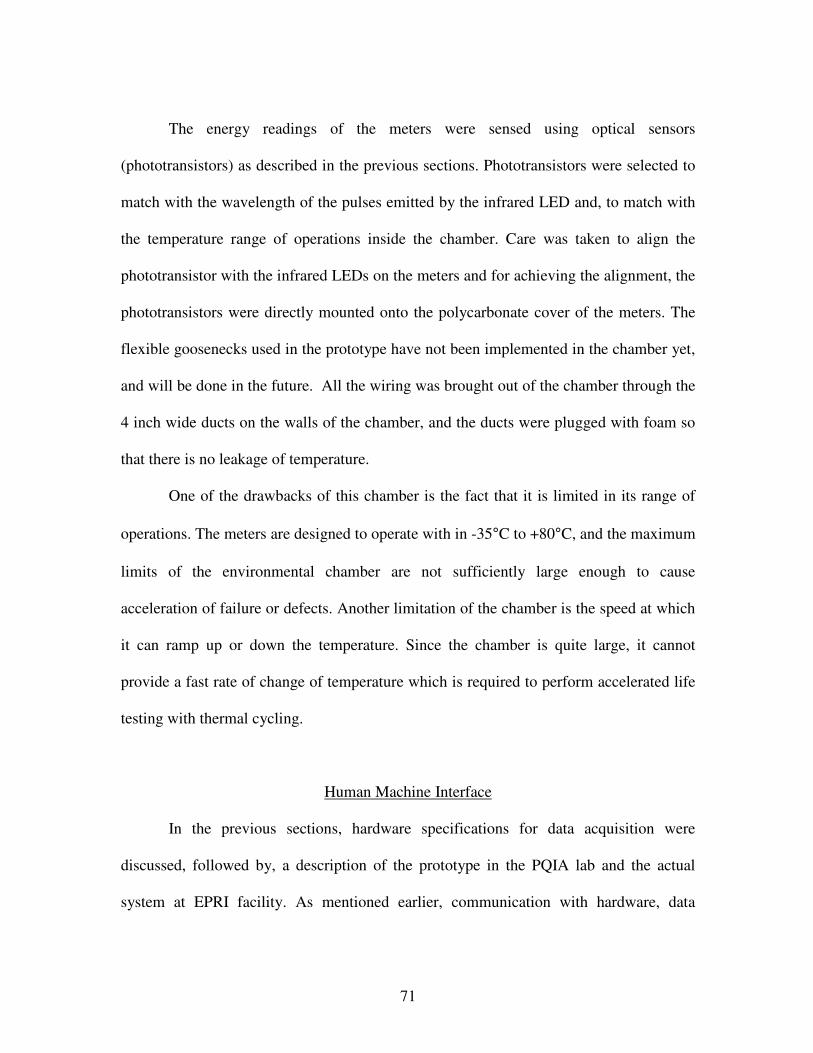
71

The energy readings of the meters were sensed using optical sensors

(phototransistors) as described in the previous sections. Phototransistors were selected to

match with the wavelength of the pulses emitted by the infrared LED and, to match with

the temperature range of operations inside the chamber. Care was taken to align the

phototransistor with the infrared LEDs on the meters and for achieving the alignment, the

phototransistors were directly mounted onto the polycarbonate cover of the meters. The

flexible goosenecks used in the prototype have not been implemented in the chamber yet,

and will be done in the future. All the wiring was brought out of the chamber through the

4 inch wide ducts on the walls of the chamber, and the ducts were plugged with foam so

that there is no leakage of temperature.

One of the drawbacks of this chamber is the fact that it is limited in its range of

operations. The meters are designed to operate with in -35°C to +80°C, and the maximum

limits of the environmental chamber are not sufficiently large enough to cause

acceleration of failure or defects. Another limitation of the chamber is the speed at which

it can ramp up or down the temperature. Since the chamber is quite large, it cannot

provide a fast rate of change of temperature which is required to perform accelerated life

testing with thermal cycling.

Human Machine Interface

In the previous sections, hardware specifications for data acquisition were

discussed, followed by, a description of the prototype in the PQIA lab and the actual

system at EPRI facility. As mentioned earlier, communication with hardware, data

72

logging, and analysis algorithms require a software program to perform real-time

calculations. Recall from Table 4.1, that the procured PXI system contains NI PXI 8106,

which is an onboard computer that runs on Windows operating system. LabVIEW 8.0 has

been installed on this system for the purpose of writing programs, and enables it to

interface with the other NI instrumentation devices that are used. LabVIEW is a dataflow

programming language whose programs are called Virtual Instruments (VIs), which are

essentially interfaces between users and instruments, and therefore also called Human

Machine Interfaces (HMI). They are very different from conventional programming

languages which are based on written lines of code.

When LabVIEW programming environment is started, the user is presented with

two windows: front panel and block diagram. On the front panel, a user can place

controls and indicators for data input and output operations. Controls, or input methods,

can be of different types such as knobs, dials, sliders, text boxes, buttons, etc. Indicators,

or output methods, comprise of progress bars, LED indicators, text boxes, graphs, etc.

When controls or indicators are placed on the front panel, the block diagram will

automatically be populated with the items that were placed on the front panel. Hardware

interface blocks and other programming functions are present as icons, which can be

placed on the block diagram, and using wires, the components can be connected such that

the data flow occurs as: Input → Programming logic → Output. This is depicted in the

Figure 4.18

73

Figure 4.18 Illustration of front panel and block diagram in LabVIEW

A VI was developed in LabVIEW for the meter testing project, and while doing

so, care was taken to make it as simple, user-friendly, and informative as possible. The

code (block diagram) for the software is given in Appendix C. In making the VI,

additional code was written, which is not a routine feature in LabVIEW, to represent all

the information on the computer screen without having to scroll or switch tabs.

On the initial execution of the HMI, a dialog box appears in which the

manufacturer details can be entered as shown in Figure 4.19.

74

Figure 4.19 Dialog box for manufacturer’s details

The manufacturer’s details include the brand, model, and the Kh constant. If the

brand and model are left unattended, the default values of “unknown” will be populated.

The Kh constants are important, since they are multiplication factors for the energy

readings of the meters; the default value of 1 will be taken, if the field is left blank.

For example, if the Kh value for a meter with a Kh constant of 7.2 is left blank,

the software will calculate energy read as 2 watt-hours for actual consumed energy of 15

watt-hours, because each pulse would then represent one watt-hour, since the default

75

value is one. This dialog box can also be accessed during execution from ‘settings’ as

explained later.

After entering the data into the dialog box and clicking the ‘OK’ button, the

program operation begins. The HMI contains four panes shown in Figure 4.20. The panes

are reference data, environmental chamber layout, user inputs, and the variable pane. The

first three panes remain constant for all pages and only the variable pane changes for each

of the pages, namely: main, meter and temperature. The default variable page is the main

or summary page, which gives a synopsis of the state of all the meters. Each meter box

has an energy output display, a power output display and an LED indicator. The energy is

calculated by accumulating pulses from the beginning of program execution and

multiplying the result by the Kh constant of the corresponding meter as entered into the

dialog box earlier. The power is calculated real-time by calculating the time period

between pulses. The LED indicator glows if that particular meter catastrophically fails or

drifts in accuracy beyond specifications. During the program execution, clicking on

summary button, in the reference data pane, changes the variable pane back to the main

page. Clicking on any meter box changes the variable page to the corresponding meter

page while the remaining three pages stay fixed.

76

Figure 4.20 Main page of the DAQ software

The components in each pane, except variable pane, are briefly explained as

follows. The variable pane changes according to the page viewed.

The reference data pane contains the following components, as seen in Figure

4.20:

• Reference meter pulses (waveform)

• Reference meter energy and power

• Elapsed time

• Settings, temperature, and summary tabs (menu)

77

The reference data pane is fixed and never hidden during any time of the

execution to ensure that the settings and reference meter data are always visible and

accessible. The waveform shows the pulses emitted by the reference calibrated meter,

which is placed outside the environmental chamber.

The reference meter energy field displays the cumulative energy seen by this

meter, in watt-hours, since the initial execution of the program. The energy seen is

determined by counting the number of pulses emitted and multiplying by the Kh constant.

Since the reference meter is not replaced during testing, its Kh constant is not capable of

being altered and is hardcoded into the program.

The reference meter power field displays the real-time power as seen by the

reference meter and is calculated by calculating the time period between the pulses. This

is then converted into power by the Equation 4.1:

pulsesbetweenperiodtime

constKhPower

×= 3600 (4.1)

The elapsed time field shows the time, in seconds, since the initial execution of

the program. The menu comprises of settings, temperature and summary buttons.

Clicking on ‘Settings’ leads to a page where the user can access the meter manufacturer

data dialog box, adjust email settings, adjust data file storage location, or reset all the

meter readings to zero. The ‘temperature’ button leads to the temperature page which is

discussed in detail later. The ‘summary’ button brings the program back to the main page

from anywhere in the program.

78

The environmental chamber layout pane also stays fixed and is never hidden

during the program execution. This pane illustrates physical layout of the meters in the

environmental chamber as shown in the previous section in Figure 4.17. Each meter is

represented by a LED indicator and turns red if the meter fails or drifts in accuracy. The

advantage of laying out the LED indicators in the same manner as the physical layout in

the chamber is that, in the event of a failure, the user can directly pinpoint the location

inside the environmental chamber because the corresponding LED indicator will turn red.

Necessary action can then be taken promptly without referring to the database of meters

to find the location in the camber.

Clicking on any LED indicator will take the user directly to the meter page and

hence facilitates moving around the HMI easily. This feature is not a standard component

of LabVIEW and additional code has been written to make the HMI more user-friendly.

The user input pane contains user inputs that make the HMI flexible and

applicable to meters of any brand. This pane consists of four user inputs as described

below:

• Error percentage

• Error duration

• Sampling rate

• Number of samples (buffer size)

The data acquisition system is built to not only to identify catastrophic failures,

but to also determine the accuracy drift of the electronic meters with time at elevated

temperatures. The HMI system continuously calculates energy accumulated by each

79

meter compares it with the reference meter, which is calibrated and placed outside the

chamber. The ‘error percentage’ input specifies the limits of error, which the system

needs to consider acceptable. For example, if error percentage is specified as 2%, then

any error within ± 2% is considered acceptable and just recorded in the log file, while

error greater than ± 2% would be considered as a catastrophic failure and the LEDs

would turn on. The reason for adding this input is to add flexibility to the system, since

different standards specify different limits of accuracy drift.

Short-term drift in accuracy for electronic meters is not uncommon, and

sometimes, meters may drift outside specified band and return immediately. This

condition cannot be considered a failure, and needs to be distinguished from actual

accuracy related failures. The ‘error duration’ input specifies a period for which the

observed error needs to be sustained in order to be considered a failure. For example, if

the error margin is specified as 2% and error duration as 1 hour (= 3600 seconds), then an

error beyond 2% sustained for one hour is considered a failure, where as, if the error

returns into the 2% margin before the time period specified, it would not be considered an

error.

The sampling rate and buffer size have been discussed in software considerations

in the previous section of this chapter. To reiterate, sampling size should be selected such

that no samples are missed by the DAQ (refer Figure 4.8). The buffer size (# of samples)

needs to be sufficiently large so that at least two pulses are captured in order to make the

waveform periodic. These settings can be adjusted real-time in the HMI which enables

checking the graphs and adjusting the sampling information accordingly.

80

Figure 4.21 Meter page of the DAQ software

Clicking on any meter in the main page, or any of the LEDs in the environmental

chamber pane changes the variable pane to the meter page of that corresponding meter as

shown in Figure 4.21. The meter page shows more details of the meter when compared to

the corresponding meter box on the main page. The items on the meter page are:

• Pulse output (waveform)

• Power and Energy fields

• Power output (waveform)

• Error percentage (waveform)

• Manufacturer’s details

81

The pulses emitted are shown in the pulse output waveform whose scales are on

autoset enabling them to adjust automatically as time changes. The power and energy

fields display the same values as in the main page box of the corresponding meter. The

power output waveform displays the last ten calculated outputs, and hence, the power

fluctuations can be observed from this plot. Error percentage waveform displays the last

ten error values, calculated by comparing with the reference meter. Manufacturer details

are automatically populated from the initial dialog box and displayed on this page. The

status LED performs the same function as the other LEDs described earlier, i.e. turn on

when a meter fails or drifts in accuracy beyond specified limits.

Figure 4.22 The temperature page of the DAQ software

82

The temperature page, as shown in Figure 4.22, can be reached by clicking on the

temperature button in the reference data pane, from where the user can monitor the

temperature of the chamber at different locations where the thermocouples have been

placed. A total of nine thermocouples can be installed and monitored using this page. An

average value of temperature can be used for the statistical calculations. The

thermometers display the instantaneous temperature. The graph shows the last ten

temperature points and automatically refreshes itself when new data is available.

Apart form the visible functions of the program on the HMI, a considerable

amount of code was written to facilitate the storage of data. The program continuously

monitors the health of the meters and generates daily and hourly reports in the form of

text files. The data includes the meter ID, average temperature, power, energy,

percentage error and status (health).

83

CHAPTER 5

TEST PLAN, RESULTS AND DISCUSSION

Test procedure

The initial test plan comprised of subjecting the electronic meters to elevated

temperatures to yield thermal related failures that could be mapped to normal usage

conditions using the Arrhenius equation. The engineers at EPRI determined the values of

the elevated temperatures to be such that they remained within the IEC specifications, of

-35 °C to 80 °C, for electricity metering [22, 23, 24, and 25]. However, the IEC

specifications do not require the meters to be in an operational state, and they only

specify that the meters to be exposed to the temperatures for a short duration of time. The

test plan developed in conjunction with EPRI consisted of three sets of tests: high

temperature tests, low temperature tests and thermal cycling tests. The details of the tests

are:

High temperature test: The high temperature test comprises of testing twenty meters (of

different brands and hence different topologies) in an environmental chamber with a

constant stress level of 80 °C under load of 30 amperes at 240 V or 9600 W. The period

of the test is 6 months. The objective of this test is to determine the effect of temperature

on discrete electronic components such as capacitors and other semiconductor devices.

One of the failure modes that is intended to be excited is the evaporation of electrolyte

84

from electrolytic capacitors present in power supplies and the signal conditioning part of

the electronic meter, and would be indicated by a drift in accuracy of the meter.

Low temperature test: The low temperature test set comprises of testing twenty meters

(again of different brands) in the environmental chamber with a constant stress level of

-35°C for a period of six months while under a load of 9600W. The objective of this test

is again to analyze a failure which is defined as a catastrophic failure or drift in meter

accuracy. Some of the failure modes are the deformation of plastic components, failure of

LCD displays, and cracking of ribbon cables present inside the meter. Electrolyte present

in capacitors also changes in viscosity, and hence changes its capacitance value, possibly

affecting the accuracy of the electronic meter.

Thermal cycling: The thermal cycling test applies stress on the meter and its components,

such as the solder joints on the printed circuit board, connectors, etc. Thermal cycle can

be obtained in environmental chambers by programming the PLC that operates the

chambers controls. The plan is to test twenty meters under load by cycling the

temperature between -35°C and 80 °C for a period of four months. Due to the limitations

of the environmental chamber at EPRI primarily due its large volume , thermal cycling

takes approximately 10 hours to change from -35°C to 80 °C and vice-versa. The dwell

time at the extreme temperatures is set to 2 hours making one complete cycle in a 24 hour

period.

85

Test results and discussion

As of the submission time of this thesis, the high temperature and low temperature

tests have been completed, and the meters showed no failures. A failure of a meter was

defined as either a catastrophic failure or a drift in accuracy greater than ± 2% as

specified by IEC and ANSI standards. These tests were conducted before the completion

of the development of the data acquisition system described in this thesis, and hence the

meters were inspected at monthly intervals by shutting down the chamber and testing the

meters using a UTEC 5800 calibration station. The results of the high temperature tests

are shown in Figure 5.1

Figure 5.1 Calibration results for high temperature tests

From Figure 5.1 it can be seen that the drift in accuracy, in the 20 meters tested,

did not show any pattern or trend, and is random. It can be observed from the figure that

the maximum drift attained was approximately 0.5%, which is well with-in the IEC and

86

ANSI standards of 2%. Therefore the life prediction analysis that was discussed in

Chapter 3 could not be used and no conclusions can be drawn regarding the predicted life

of the electronic meters.

Thermal cycling tests will commence in September 2008 and the results will be

available for analysis in December 2008, beyond the submission date of this thesis. Since

no failure data from thermal tests are available as of today, no analysis can be performed.

From the analysis of the results the following conclusions regarding the high

temperature and low temperature tests can be drawn:

• The present test results only confirm that the electronic meters that were tested

conform to the ANSI and IEC standards of -35°C to 80 °C. They do not provide

any failure data or insight into the failure mechanism.

• The meters were designed for a temperature range of -35°C to 85 °C and hence

testing within the range of -35°C to 80 °C may not yield results because there is

negligible acceleration in the failure mode

• In order to obtain failure data, two options are available: testing at higher levels of

thermal stress, or testing for a longer duration of time.

• In order to obtain useful information regarding the life of the meters, failures from

identical electronic meters is required, and the test plan comprising of testing

small samples of different brands will not yield any useful information.

87

Recommended test plan

In order to carry out the life prediction analysis, obtaining failure data is essential.

The following recommended strategies may improve the probability of obtaining data in

a timely fashion:

1. Conduct a pilot test with a few samples to gain insight into the failure mechanism.

Such pilot test can provide useful information in deciding the number of samples

to tests and appropriate stress levels. For example, a pilot test conducted on a few

samples showed that a stress level of 125 °C induced failures in the control

transformer for a particular brand of meters.

2. A decision needs to be made for the number of samples to be tested. The failure

distribution parameters can be more closely predicted when a large number of

failure times are available. Since we cannot expect all the meters to fail, a large

number of samples must be tested. The samples decided to be tested should be of

the same brand so that the failure mode occurs in all of them. For example, if 20

times-to-failure are required, at least 40 meters should be tested.

3. Two temperature levels need to be decided based on the pilot tests. The pilot test

conducted at 125 °C showed that it would be sufficient to induced failures. 125 °C

was chosen because it is 150% of the design stress level and is neither too less nor

falls into the destruct levels. Hence 125 °C can be chosen as one elevated level. In

order to map the relationship to the usage level another mid-level temperature is

required and chosen as 100 °C. The DAQ can be used to continuously monitor the

meters while testing at these temperatures.

88

4. More samples should be tested at lower temperature (100°C) so that more failures

may be observed. The probability of failure is greater at high temperatures, and

hence testing a few samples at higher temperatures is advisable. The decision on

distribution of the samples relies on previous distribution data. For example, if

100 meters were available for testing, and 20 meters are required to fail at each

stress level, then 30 meters should be placed at 125°C and 70 meters at 100°C.

5. For thermal cycling test, a steeper ramp rate is required to induce thermal stress

on solder joints. This is a limitation of the environmental chamber and hence a

new smaller chamber may need to be procured.

89

CHAPTER 6

ANALYSIS USING EXAMPLES

Introduction

Lab testing of electronic revenue meters began in August 2007 and two sets of

tests have been conducted as of the submission of this thesis. The first test was conducted

at a constant temperature of 80 °C, before the development of the DAQ described in

Chapter 4, and the meter inspections were done manually at the end of each month for a

period of six months. At the end of the six month period, none of the meters had failed,

and the drift in accuracy was negligible and random. The second test was conducted at -

35°C, also for a period of six months, and did not yield any failures. The reason for lack

of failures or significant deviation in accuracy was determined to be the fact that the

meters were designed for the test temperature range being used, and to observe any

failures, either the stress or the testing time had to be increased significantly.

Since there is no data, life prediction analysis could not be performed on the

meters. The reason for the lack of data was found to be the levels of stress used, and

resulted in negligible acceleration of the failure mode. These stress levels were decided

by EPRI engineers prior to this thesis. For the purpose of demonstration of the analysis

procedure, two examples are provided in this chapter, which will illustrate the concepts

explained in Chapter 3. The first problem deals with failure data analysis, while the

second one analyzes degradation data.

90

Failure data analysis

In the following problem, the data is obtained from accelerated testing

experiments conducted on distribution system cable insulation, and the objective is to

determine the life of electric cable insulation under design conditions. This data is taken

from the datasets provided by Minitab software. When test results for the accelerated life

tests of electronic meters are available, similar analysis will yield estimates of operational

lifetime of the meters in the field.

Forty cable insulation specimens were subjected to elevated temperatures (twenty

at 130 °C and the other twenty at 110 °C). These temperatures are approximately 50%

greater than design stress (80 °C), which is acceptable, and do not lie within destruct

levels, where definite failures would occur and yield no useful information. The data

comes from a traditional test plan, because of the equal distribution of specimens between

the two stress levels. In an optimal plan, specimens would be distributed as per some

calculated statistic, which usually involves analysis of previously acquired life-data of the

same component, and expert opinion. The insulation on the specimens is continuously

monitored and times-to failure data is shown in Table 6.1.

91

Table 6.1 Failure data of insulation specimens

Temperature

(°C)

Failure

Time

(Hours) Censor

Design

(°C)

Temperature

(°C)

Failure

Time

(Hours) Censor

Design

(°C)

130 2214 F 80 110 7336 C 80

130 3128 F 110 8702 F

130 3147 F 110 11143 C

130 3308 F 110 11769 F

130 3545 F 110 12090 F

130 3620 C 110 13218 F

130 3987 F 110 13513 F

130 4348 F 110 13673 F

130 4373 F 110 14482 F

130 4735 C 110 16289 F

130 4925 F 110 17610 F

130 5117 F 110 17784 F

130 5351 F 110 17822 F

130 5355 F 110 18397 F

130 6226 F 110 18806 F

130 6947 F 110 20975 F

130 7304 F 110 21900 C

130 7919 F 110 21900 C

130 8290 F 110 21900 C

130 10183 F 110 21900 C

The test is stopped after 21900 hours, possibly because of a managerial decision,

and thus resulting in data being right censored. Apart from the censored data after 21900

hours, there are some randomly censored data, for unknown reasons, that are identified

by the letter C in the Censor column in the Table 6.1.

Once the data is accumulated, the analysis method follows the steps explained in

Chapter 3 and can be depicted by the flowchart as follows:

92

Figure 6.1 Flowchart of statistical analysis for accelerated life tests

93

As indicated by the flowchart, the first step in analyzing failure data is to draw

histograms, which would provide insight into the underlying distribution. In drawing a

histogram, it is important to select appropriate bin sizes, and selecting either larger or

smaller sizes will distort the shape of the distribution. There is no “correct” method in

selecting bin sizes, and many mathematicians have proposed different empirical

equations for the selection. The software used to plot the graphs in this chapter is Minitab

statistical analysis software version 15 [38].

2000016000120008000

25

20

15

10

5

0

Time (hours)

Per

cen

t o

f fa

iled

sp

ecim

ens

Figure 6.2 Histogram of the failure data at 110 °C

94

100008000600040002000

30

25

20

15

10

5

0

Time (hours)

Per

cent

of

faile

d s

pec

imen

s

Figure 6.3 Histogram of the failure data at 130 °C

From the histograms above, the data can be suspected to be from normal,

lognormal, or Weibull distributions. However, other data distributions, such as

exponential, can also be used, and then tested for goodness of fit. Since the data is

censored, Maximum Likelihood methods are used to determine the parameters of the

distribution. Recall from Chapter 3 that the likelihood estimator is defined as:

∏=

=N

i

kiN AAAAxfAAAAxxxxL1

210k210321 ),...,,,;(),...,,,|,...,,,( (6.1)

For an exponential distribution, estimation of the parameters using MLE is shown

as follows. The pdf of an exponential distribution is given by:

tetf λλ −=)( (6.2)

Applying Equation 6.1, we get:

95

∏=

−=N

i

tetttL1

k21 ),...,,|( λλλ

∑×= =

−N

i

itN e 1

λλ (6.3)

Taking the natural logarithm to get the log likelihood estimator, we get:

∑=

−==ΛN

i

itNL1

)ln(ln λλ (6.4)

For the log likelihood estimator to be maximum, we find the partial derivative

with respect to λ and equate to zero. This will give us an estimate of λ as:

∑=

=N

i

it

N

1

λ (6.5)

Similarly the estimates of other probability distributions can be determined and is

generally done using software as in this problem.

The probability plots for the distributions are shown in Figures 6.3 and 6.4 for

110 °C and 130 °C respectively. The goodness of fit can be determined either graphically

or by using the Anderson-Darling (AD). Recall from Chapter 3, that the AD statistic is

determined by the equation:

SNA −−=2 (6.6)

where ∑=

−+−+−=N

k

kNk TFTFN

kS

1

1 ))](1ln()([ln12

96

This is a very tedious calculation, and generally software is used to calculate the

statistic. The test statistics for the distributions in this problem are tabulated in Table 6.2

2000010000

90

50

10

1

Time

Percent

2000010000

99

90

50

10

1

Time

Percent

300002000010000

99

90

50

10

1

Time

Percent

100000100001000100

90

50

10

1

Time

Percent

Weibull Lognormal

Normal Exponential

Figure 6.4 Probability plots of the failure data at 110 °C

1000050002000

90

50

10

1

Time

Percent

1000050002000

99

90

50

10

1

Time

Percent

1000050000

99

90

50

10

1

Time

Percent

100001000100

90

50

10

1

Time

Percent

Weibull Lognormal

Normal Exponential

Figure 6.5 Probability plots of the failure data at 130 °C

97

Table 6.2 Anderson Darling test statistic values

Distribution AD statistic

110 °C 130 °C

Weibull 23.12 1.12

Lognormal 23.10 1.02

Normal 23.11 1.23

Exponential 24.79 3.64

In order to determine goodness of fit graphically, the residuals in the plots in

Figures 6.4 and 6.5 need to be carefully observed where the straight line describes the

cumulative distribution function form fitting the dataset, on a linearized scale, and the

dots are residuals (deviations) of each data point. If all the residual points lie on or around

the straight line, then it is a good fit, where as if they are far apart (for example

exponential), then the data does not come from that type of distribution. Alternately, by

using the Anderson-Darling (AD) test statistic, the goodness of fit can be determined.

The AD test statistic is calculated from Equation 3.13 in Chapter 3, and its value should

be within specified range of values found in literature for each type of distribution. When

the range of values is not available, the distribution with the lowest value of AD statistic

fits the data the best. From Table 6.2, it is observed that lognormal distribution describes

the data in the problem more closely than any other distribution because the AD value is

the least. The mean and standard deviation are determined at each stress level by using

maximum likelihood estimation.

The estimates of the lognormal distribution at both temperatures are calculated

using software and shown in Figures 6.6 and 6.7

98

Figure 6.6 Lognormal characteristics of the failure data at 110 °C

Figure 6.7 Lognormal characteristics of the failure data at 130 °C

From the statistics displayed in Figures 6.6 and 6.7, it observed that the mean life

of insulation is 17886 hours at 110 °C and 5434.49 hours at 130 °C. Since the stress is

temperature, Arrhenius model can be used to extrapolate life to design conditions.

Activation energy for the Arrhenius equation can be calculated from the Equation 6.7

99

−

=

21

21

2

1ln.TT

TT

L

LkEA (6.7)

where L1 and T1 correspond to life and temperature at one elevated stress

L2 and T2 correspond to life and temperature at a different elevated stress

k is the Boltzmann’s constant (8.623 x 105)

Substituting the results obtained earlier, we get EA = 0.00669 eV. Using this

value, life at any other stress can be determined using Equation 5.2

−

= SO

A

TTk

E

SO eLL

11

(6.8)

where LO and TO correspond to life and temperature at the design stress level

LS and TS correspond to life and temperature at the elevated stress level

k is the Boltzmann’s constant (8.623 x 105)

The results for such a calculation have been performed using software and the

plot is shown in Figure 6.8

410400390380370360350

100000

10000

1000

Stress (temperature)

Lif

e (h

ou

rs)

Figure 6.8 Arrhenius plot for cable insulation

100

From the plot in Figure 6.8, the predicted design life for cable insulation at design

temperature of 80°C is 121,368 hours or approximately 13.8 years.

Degradation data analysis

The analysis previously conducted describes the analysis method for failure data.

Some products and components show degradation characteristics, and in those situations,

time and money can be saved by testing the specimens for degradation parameters rather

than failures. Degradation beyond a limit can be considered a failure because the device

would be rendered useless after those degradation levels. Some of the examples of

degradation are light intensity of LEDs, strength of adhesive bonds, etc. Data for

degradation analysis of 24 LEDs is shown in the Table 6.3. The accelerating stress is

current and the output light intensity decreases with time. The LED’s are inspected after

every 50 hours up to 250 hours. If this was a failure data test, the specimens would have

taken longer to fail and hence prove expensive. Degradation of light intensity below 50

units is considered a failure.

101

Table 6.3 Degradation data of LEDs

inspection (hours)

Light intensity

current (mA) unit id

inspection (hours)

Light intensity

current (mA) unit id

50 86.6 40 1 50 95.1 35 13

100 78.7 40 1 100 86 35 13

150 76 40 1 150 77.6 35 13

200 71.6 40 1 200 70 35 13

250 68 40 1 250 66.7 35 13

50 82.1 40 2 50 93.3 35 14

100 71.4 40 2 100 87.1 35 14

150 65.4 40 2 150 79.7 35 14

200 61.7 40 2 200 74.3 35 14

250 58 40 2 250 73 35 14

50 82.7 40 3 50 98.3 35 15

100 70.3 40 3 100 92.4 35 15

150 64 40 3 150 89 35 15

200 61.3 40 3 200 84.3 35 15

250 59.3 40 3 250 83 35 15

50 79.8 40 4 50 96.6 35 16

100 68.3 40 4 100 88.2 35 16

150 62.3 40 4 150 85.1 35 16

200 60 40 4 200 81.4 35 16

250 59 40 4 250 78.6 35 16

50 75.1 40 5 50 95.8 35 17

100 66.7 40 5 100 89 35 17

150 62.8 40 5 150 84 35 17

200 59 40 5 200 81 35 17

250 54 40 5 250 80 35 17

50 83.7 40 6 50 94 35 18

100 74 40 6 100 82.4 35 18

150 67.4 40 6 150 77.4 35 18

200 63 40 6 200 71.7 35 18

250 61.3 40 6 250 70.6 35 18

50 73 40 7 50 88.2 35 19

100 65 40 7 100 78.7 35 19

150 60.7 40 7 150 75 35 19

200 58.3 40 7 200 70 35 19

250 58 40 7 250 69.3 35 19

50 86.2 40 8 50 86.7 35 20

100 67.6 40 8 100 78 35 20

150 62.7 40 8 150 73.3 35 20

200 60 40 8 200 68.7 35 20

250 59.7 40 8 250 67.3 35 20

50 81.2 40 9 50 89 35 21

100 65 40 9 100 80 35 21

150 60.6 40 9 150 76.3 35 21

200 59.3 40 9 200 72.3 35 21

250 57.3 40 9 250 71.3 35 21

50 66.8 40 10 50 96.2 35 22

100 63.3 40 10 100 86.5 35 22

150 59.3 40 10 150 81.4 35 22

200 57.3 40 10 200 74.5 35 22

250 56.5 40 10 250 74.2 35 22

50 66.1 40 11 50 97.5 35 23

100 64.2 40 11 100 84.5 35 23

150 59.4 40 11 150 81 35 23

200 58 40 11 200 75 35 23

250 55.3 40 11 250 74.1 35 23

50 76.5 40 12 50 92.4 35 24

100 61.7 40 12 100 85.4 35 24

150 61.3 40 12 150 80 35 24

200 59.7 40 12 200 73.3 35 24

250 56 40 12 250 71.5 35 24

102

In degradation analysis, basic mathematical models are used to extrapolate the

performance measurements over time to the point where the product would have

degraded beyond critical value. Once this has been determined, analysis can be done with

standard life data analysis techniques. For the data above, a linear model is used and the

following graph in Figure 6.9 is obtained

ReliaSoft ALTA 7 - www.ReliaSoft.com

Degradation vs Time

Time, (t)

Degradation

40.000 600.000152.000 264.000 376.000 488.00030.000

100.000

44.000

58.000

72.000

86.000

Linear Fit

1Data PointsDegradation

2Data PointsDegradation

3Data PointsDegradation

4Data PointsDegradation

5Data PointsDegradation

6Data PointsDegradation

9Data PointsDegradation

10Data PointsDegradation

11Data PointsDegradation

12Data PointsDegradation

13Data PointsDegradation

14

Figure 6.9 Degradation data

From Figure 6.9, most of the LEDs fail as they cross the thick horizontal pink line

at 50 units. The points at which they do so are considered their failure times and standard

failure data analysis is then performed as performed in the previous example. Recall from

Chapter 3 that the inverse power law can be used to determine the relation since the

accelerating stress is not temperature. Since the stress in this case is current, the inverse

103

power law can be used to map the life at operating with 40 mA to a design level of 25

mA. The On solving the problem using the approach shown in the previous example,

Figure 6.10 is obtained. It shows the life vs. stress. From the plot, the predicted life at

design current of 25 amperes is 1346 hours.

ReliaSoft ALTA 7 - www.ReliaSoft.com

Life vs Stress

Beta=5.9475; K=3.2971E-8; n=3.0899

Amps

Life

10.000 100.000100.000

10000.000

1000.000

Life

Data 1Inverse Power LawWeibull28F=24 | S=0

Eta Line35

Stress Level PointsEta PointImposed Pdf

40Stress Level PointsEta PointImposed Pdf

harish chaluvadiclemson university8/14/200811:06:08 AM

Figure 6.10 Inverse power law plot showing stress vs. life

104

CHAPTER 7

CONCLUSION

Traditionally, electricity consumption was measured using electromechanical

watt-hour meters. Many meters, across America, have reached the wear-out stage of their

lifespan and require replacements. In the next few years, utilities all over the country

intend to replace these old and aging electromechanical meters with state-of-the-art

electronic ones on a large scale [35]. Doing so could improve metering accuracy, add

security, allow communications (AMI), and facilitate demand response operations in

distribution systems. However, the reliability of electronic components has been a

concern and many experts believe that the electronic meters will not survive as long as

their electromechanical predecessors [35].

This thesis provides a methodology for the prediction of life of electronic meters

using accelerated life tests. At first, fundamentals of meter operation are discussed, since

knowledge of the construction and operation of the electronic meters is essential to

pursue the project further. Operational features and gear ratio constants of traditional

electromechanical meters are also discussed because terminology related to calibration is

inherited from these electromechanical meters to the new electronic ones.

This is followed by a literature review of accelerated test methods and models.

Different data types and corresponding analysis methods are discussed. Failure time

distributions along with goodness-of-fit tests are also reviewed. Finally the various life-

105

stress relationships that are used to map estimates at high stress conditions to the usage

conditions, for different types of stresses, are discussed.

Meter failures in the field that would generally occur over many years can be

observed at a faster rate by operating them in environmental chambers at elevated stress

conditions by a technique known as accelerated life testing (ALT). The methods of

analyzing the resulting failure data were also discussed.

The manual inspection of meters on a monthly basis would provide only censored

data and would be inadequate for life analysis prediction. A Data Acquisition system

(DAQ) was developed to extract data from the interiors of the inaccessible environmental

chambers. The DAQ was required to extract information regarding the health of the

meters and the temperature from the interior of the environmental chamber. At first, the

required design specifications for proper functionality of the DAQ are identified. Based

on these specifications, sensors, both infrared phototransistors and thermocouples, are

selected. This is followed by an explanation of the details of the instrumentation devices

developed for data acquisition. Finally, a Human Machine Interface (HMI), that is used to

interface the data acquisition system with software, is built using LabVIEW. The benefits

of the layout of the HMI and its functionality have also been illustrated in detail.

In constructing the HMI, a few meters were required to be in an operational state

to gain insight into the pulse characteristics i.e., wavelength, width, and rate of

occurrence of the pulses. Methods of making the DAQ flexible for operation with any

brand of meters were also to be determined. In order to accomplish these tasks, a

prototype had to be constructed in Clemson University’s PQIA lab that would mimic the

106

actual test setup at the EPRI facility. The details of the prototype have been discussed in

detail.

Then a description of the features and limitations of the test set-up used at the

EPRI facility to conduct ALTs were provided. The environmental chamber that is being

used at EPRI facility was found to be limited in its operation. In the future, the system

needs to be expanded by increasing the environmental chamber’s heating and

refrigeration capability in order to obtain failure data in a timely fashion.

After six months of testing at a constant stress of 80 °C, no failures were observed

in the 20 meters that were being tested. Degradation data revealed the meters to be within

the IEC and ANSI design specifications. The EPRI test plan was inadequate for inducing

thermal-related failures in the electronic meters, and thus life prediction analysis could

not be carried out. The reasons for this have been discussed and remedies are listed in

Chapter 5.

Since no failure data was observed during the time devoted to this project, the

analysis method determined to predict the life of the electronic watthour meters have

been illustrated using data from the literature. Two methods of analysis, i.e., traditional

failure data analysis and degradation analysis have been illustrated using failure data

from cable insulation specimens and LED specimens respectively. When the failure data

for the electronic meters is available from future experiments, it can be used, with

minimal alterations to the model, to obtain the estimate of life as illustrated using the

examples.

107

Future work

The data acquisition system described in this thesis was designed with the

capability of being expanded, as more phototransistors and thermocouples can be

attached when required. Life-stress relationships for stresses other than temperature have

also been described in the Chapter 3 and could yield valuable life related information.

Lab testing at 80 °C and -35 °C did not reveal any failures. The reason for lack of failures

was determined to be the levels of stresses. Both 80 °C and -35 °C fall within the IEC

design specifications of electronic revenue meters [22], and in order to observe failures,

either the stress level or test duration will need to be increased. Improvements in the test

plans by increasing the stress levels can yield better results and these recommendations

were made to EPRI.

In the future, a temperature cycling test is to commence with temperature cycled

between the two extremes – 80 °C and -35 °C. The test will be conducted for a period of

four months and the results, for analysis, will be available by the end of December 2008.

The Coffin-Mason life-stress relationship can be used to map the results, if any, to usage

level conditions. However, it is unlikely that failures will result from this test because the

rate of increase of temperature in the chamber is not high enough to induce thermal

shock. The reason for the slow rate of increase was concluded to be because of the large

size of the chamber.

Once the dependence of life on temperature is determined, life–stress

relationships with other stresses that act on electronic meters in the field should be

investigated. In a future phase of this sponsored project, an additional stress, such as

108

voltage will be added. This will give the correlation between life and both the stresses

acting simultaneously on the meter and thus mimic the actual conditions under which the

meter operates in the field more closely. The data acquisition system has been made

flexible to accommodate any brand of meters and different types of stresses, and thus can

be used for all future testing.

109

APPENDICES

110

Appendix A

NI SCB 68 breakout board pinout diagram

Figure A.1 Pin-out diagram of SCB 68 for NI 653X series

(Source: NI SCB 68 user manual)

111

Appendix B

Type T thermocouple coefficients

Temperature range : -200 to 0 °C Temperature range : 0 to 400 °C

Voltage range : -5.6 to 0 mV Voltage range : 0 to 20.87 mV

coefficients

coefficients

a0

0 a0

0

a1

25.949192 a1

25.928

a2

-0.21316967 a2

-0.7602961

a3

0.79018692 a3

0.04637791

a4

0.42527777 a4

-0.002165394

a5

0.13304473 a5

6.04814E-05

a6

0.020241446 a6

-7.29342E-07

a7

0.001266817 a7

0

Table B.1 Coefficients for voltage to temperature conversion of

T type thermocouple (Source: www.nist.gov)

n

nEaEaEaEaEaaT ++++++= ..............4

4

3

3

2

210

Where a0, a1, a2 ....an are coefficients from the Table B.1

E is the emf or voltage observed in mV

T is the temperature in °C

112

Appendix C

LabVIEW program

113

114

115

116

117

REFERENCES

[1] A brief history of meter companies and meter evolution, Website :

http://watthourmeters.com/history.html (accessed 07/04/2008).

[2] United States Energy Policy Act 2005, Website: http://www.epa.gov (accessed

07/08/08).

[3] W. B. Nelson, Accelerated Testing: Statistical models, Test Plans and Data

Analysis, 2nd ed., New York NY: John Wiley and Sons, 1990.

[4] E. A. Elsayed, Reliability Engineering, Pearson Education, 1996.

[5] W.Q Meeker and L.A Escobar, Statistical Methods for Reliability Data, New York

NY: John Wiley and Sons, 1998.

[6] United States Bureau of reclamation, Watt-hour meter maintenance and testing,

FIST 3-10, 1992.

[7] N.Wan and K. Manning, “Exceeding 60-Year Life Expectancy from an Electronic

Energy Meter”, Metering Asia Pacific Conference, Feb 2001.

[8] American National Standards Institute, Code for electricity metering, C12.1, 2001.

[9] E. Suhir, “Accelerated Life Testing in Photonics Packaging: Objectives, Role,

Attributes, Challenges, Pitfalls, Predictive Models, and Interaction with Other

Accelerated Stress Categories”, SPIE, 2002.

[10] NIST/SEMATECH e-Handbook of Statistical Methods, Website:

http://www.itl.nist.gov/div898/handbook/ (accessed 07/08/08).

[11] H. Cui, “Accelerated Temperature Cycle Test and Coffin-Manson Model for

Electronic Packaging”, IEEE RAMS, 2005.

[12] L. A. Escobar and W. Q. Meeker, “Statistical Prediction Based on Censored Life

Data”, Technometrics, vol. 41, no. 2, pp. 113-124, May 1999.

[13] W. B. Nelson, “Analysis of Accelerated Life Test Data – Part I: The Arrhenius

Model and Graphical Methods”, IEEE Transactions on Electrical Insulation, vol.

EI-6, no. 4, pp. 165-181, Dec. 1971.

118

[14] W. B. Nelson, “Analysis of Accelerated Life Test Data – Part II: Numerical

Methods and Test Planning”, IEEE Transactions on Electrical Insulation, vol. EI-

7, no. 1, pp. 36-55, Dec. 1972.

[15] W. B. Nelson, “Analysis of Accelerated Life Test Data – Part III: Product

Comparisons and Checks on the Validity of the Model and the Data”, IEEE

Transactions on Electrical Insulation, vol. EI-7, no. 2, pp. 99-119, Jun. 1972.

[16] W. Q. Meeker and G. J. Hahn , “A Comparison of Accelerated Test Plans to

Estimate the Survival Probability at a Design Stress”, Technometrics, vol. 20, no.

3, pp. 245-247, Aug. 1978.

[17] W.Q Meeker and L.A Escobar, “Using Accelerated Tests to Predict Service Life in

Highly-Variable Environments”, Invited 71: Quality and reliability improvement,

vol. 21, no. 4, pp. 245-247, Aug. 1980.

[18] W.Q Meeker and L.A Escobar, “Statistical Methods for Reliability Data Using

SAS Software”, Technometrics, vol. 20, no. 3, pp. 245-247, Aug. 1978.

[19] J. W. Park, “Case Studies on the Accelerated Life Tests for the Semiconductor

Devices Tests Devices”, The 16th ISRC Workshop

[20] W. M. Shepard and A. G. Jones, The Watthour Meter, Technical publishing

company, 1910.

[21] Handbook for Electricity Metering, Edison Electric Institute, 9th

edition, Aug.

1999.

[22] Electricity metering equipment (AC) – General requirements, tests and test

conditions –Part 11: Metering equipment, International Electrotechnical

Commission, 62052-11, 2003.

[23] Electricity metering equipment (AC) – Particular requirements – Part 21: Static

meters for active energy (classes 1 and 2), International Electrotechnical

Commission, 62053-21, 2003.

[24] Electricity metering equipment (AC) – Particular requirements – Part 11:

Electromechanical meters for active energy (classes 0.5, 1 and 2), International

Electrotechnical Commission, 62053-11, 2003.

[25] Electricity metering equipment (AC) – Particular requirements – Part 31: Pulse

output devices for electromechanical and electronic meters (two wires only),

International Electrotechnical Commission, 62053-31, 1998.

119

[26] J. Sethuraman and N. D. Singpurwalla, “Testing for Hypotheses for Distributions

in Accelerated Life Tests”, Journal of the American Statistical Association, vol.

77, no. 377, Theory and Methods Section, Mar. 1982.

[27] Analog Devices Reliability Handbook. Website: http://www.analog.com (accessed

07/05/2008).

[28] V. Ricci, Fitting Distributions with R, Release 0.4, Feb. 2005.

[29] N. H. Criscimagna, “Accelerated Testing”, Selected Topics in Assurance Related

Technologies, vol. 6, no. 4, Apr. 1999.

[30] Life data Analysis reference, Website: www.weibull.com (accessed 07/04/2008),

Updated: Apr. 2007.

[31] Accelerated Life Testing reference, Website: www.weibull.com (accessed

07/04/2008), Updated: Apr. 2007.

[32] C. R. Yang and J. T. Kim, “Temperature Accelerated Life Test (ALT) at the

Circuit Board Level”, IEEE International Electronics Manufacturing Technology

Symposium, Apr. 1995.

[33] W. J. Minford, Accelerated Life Testing and Reliability of High K Multilayer

Ceramic Capacitors”, IEEE transactions on Components, Hybrids, Manufacturing

Technology, vol. CHMT-5, pp. 297-300, Sep 1982.

[34] J. P. Rooney, “Aging in Electronic Systems”, Proceedings of the Annual

Reliability and Maintainability Symposium, pp. 293-299, Aug. 1999.

[35] Accelerated Life Testing of Solid-State Residential Meters: Technical Update,

EPRI, Palo Alto, CA: 2006. 1012440.

[36] Obsolescence Planning of Domestic Electronic Meters. EPRI, Palo Alto, CA:

2006. 1012441.

[37] Accelerated Life Testing of Domestic Solid-State Residential Meters. EPRI, Palo

Alto, CA: 2007. 1013968.