Accel Notes
66
SLAC-75 A First- and Second-Order Matrix Theory for the Design of Beam Transport Systems and Char ed Particle Spectrometers Karl L. Brown SLAC R ep ort - 75 J une 1982 — Under contract wth the Depar tment of Ener gy Con t ract DE- AC03 - 7 6 S F O 051 5 STANFORD L INEAR ACCELERATOR CENTER Stanf ord Uni versi ty . St anf or d Cal i f or ni a
Transcript of Accel Notes

5/12/2018 Accel Notes - slidepdf.com
http://slidepdf.com/reader/full/accel-notes 1/66
SLAC-75
A First- and Second-Order Matrix Theory
for the Design of Beam Transport Systems and
Charged Particle Spectrometers
Ka r l L . B r o wn
SLAC Re p o r t - 7 5
J u n e 1 9 8 2
—
Un d e r c o n t r a c t wi t h t h e
De p a r t me n t o f E n e r g y
Co n t r a c t DE - A C0 3 - 7 6 SF O0 5 1 5
ST ANF ORD L I NEAR ACCEL ERAT OR CENT ER
S t a n f o r d Un i v e r s i t y . S t a n f o r d Ca l i f o r n i a
5/12/2018 Accel Notes - slidepdf.com
http://slidepdf.com/reader/full/accel-notes 2/66
This document and the material and data contained therein, was devel-oped under sponsorship of the United States Government. Neither the
United States nor the Department of Energy, nor the Leland Stanford
Junior University, nor their employees, nor their respective contrac-
tors subcontractors, or their employees, makes any warranty, express
or implied, or assumes any liability or responsibility for accuracy,
completeness or usefulness of any information, apparatus, product or
process disclosed, or represents that its use will not infringe pri-
vately-owned rights. Mention of any product, its manufacturer, or
suppliers shall not, nor is it intended to, imply approval, disap-
proval, or fitness for any particular use. A royalty-free, nonex-
clusive right to use and disseminate same for any purpose whatsoever,
is expressly reserved to the United States and the University.
I
i
1
I
I
$
7/82

5/12/2018 Accel Notes - slidepdf.com
http://slidepdf.com/reader/full/accel-notes 3/66
SLAC -75, Rev.4UC-28(M)
A First- and Second-Order Matrix Theory
for the Design of Beam Transport Systems and
Charged Particle Spectrometers*+
KARL L. BROWN
Slan fordLinear.accelerator Center ,
S tan ford Universi ty , S tan ford , Cal !~orn ia
June 1982
Contents
1. Introduction .
11. A General First- and Second-Order Theory of Beam Transport Optics
1. The Vector Differential Equation of Motion .
2. The Coordinate System . . .
3. Expanded Form ofa Magnetic Field Having Median Plane Symmetry
4. Field Expansion to Second Order Only . .
5. Identification oft~ and ~ with Pure Quadruple and Sextupole Fields
6. The Equations of Motion in Their Final Form to Second Order7. The Description of the Trajectories and the Coefficients of the
Taylor’s Expansion . ‘ . . . .
8. Transformation from Curvilinear Coordinates to a Rectangular
Coordinate System and TRANSPORT Notation .
9. First- and SecQnd-Order Ma(rix Formalism of Beam Transport Optics
I Il. Reduction of the General First- and Second-Order Theory to the Case of
theldeal Magnet.
1. Matrix Elements for a Pure Quadruple Field .
2. Matrix Elements for a Pure Sextupole Field .
3. First- and Second-Order Matrix Elements for a Curved, Inclined
Magnetic Field Boundary . .
4. Matrix Elements for a Drift DistanceIV. Some Useful First-Order Optical Results Derived from the General
Theory of Section 11 .
1. First-Order Dispersion
72
78
82
82
85
89
91
91
93
98
102
107
114
115
16
18
19
20
2. First-Order Path Length I20
* Work suppor ted by the QepaFtment of Ener gy, con t ract DE-AC03-76SFO0515.
t Permission t o repr in t th is a r t icle, published in Advances in Par t icle
P hysics J ou rn al, gran ted by J ohn Wiley and Sons, Inc.
5/12/2018 Accel Notes - slidepdf.com
http://slidepdf.com/reader/full/accel-notes 4/66
72 K. L. BROWN
A. Achromaticity .
B. Isochronicity
3. First-Order Imaging4. Magnification
5. First-Order Momentum Resolution
6. Zero Dispersion
7. Focal Length. .
8. Evaluation of the First-Order Matrix for Ideal Magnets9, The R Matrix Transformed to the Principal Planes
V. Some General Second-Order Theorems Derived from the General
Theory of Section 11 .
1. Optical Symmetries in )Z= + Magnetic SystemsV I , An Approximate Evaluation of the Second-Order Aberrations for High-
Energy Physics
l. Case I .2. Case II. .
3. Case III .
References . . . . . . . .
I. Introduction
121
121
121122
122
1~~
123
123
124
129
132133
133
134
Since the invention of the alternating gradient principle and the
subsequent design of the Brookhaven and CERN proton-synchrotrons
based on this principle, there has been a rapid evolution of the mathe-
matical and physical techniques applicable to charged particle optics.
In this report a matrix algebra formalism will be used to develop the
essential principles governing the design of charged particle beam
transport systems, with a particular emphasis on the design of high-
energy magnetic spectrometers. A notation introduced by John Streib(l)
has been found to be ~seful in conveying the essential physical principles
dictating the design of such beam transport systems. ln particular to
first order, the momentum dispersion, the momentum resolution, the
particle path length, and the necessary and sufficient conditions for zero
dispersion, achromaticity, and isochronicity may all be expressed as
simple integrals of particular first-order trajectories (matrix elements)
characterizing a system.
This formulation provides direct physical insight into the design of
beam transport systems and charged particle spectrometers. An intuitive
grasp of the mechanism of second-order aberrations also results from
this formalism; for example, the effects of magnetic symmetry on the
minimization or elimination ofsecond-order aberrations is immediately
apparent.

5/12/2018 Accel Notes - slidepdf.com
http://slidepdf.com/reader/full/accel-notes 5/66
SYSTEM
The equations of
formalism tintroduced,
Physical examples will
AND SPECTROMETER DESIGN 73
motion will be derived and then the matrix
developed, and evolved into useful theorems.
be given to illustrate the applicability of the
formalism to the design of specific spectrometers. It is hoped that theinformation supplied will provide the reader with the necessary tools so
that he can design any beam transport system or spectrometer suited to
his particular needs.
The theory has been developed to second order in a Taylor expan-
sion about a central trajectory, characterizing the system. This seems to
be adequate for most high-energy physics applications. For studying
details beyond second order, we have found computer ray tracing
programs to be the best technique for verification of matrix calculations,
and as a means for further refinement of the optics if needed.
.ln the design of actual systems for high-energy beam transport
applications, it has proved convenient to express the results via a multi-
polcexpansion about a central trajectory. in this expansion, the constant
tcrrn proportional to the Iicld strc]lgth at the ccntra] trajectory is the
dipole term. The term proporti(~n~~l to the first derivative of the field
(with respect to the transverse dinlcnsi(lns) about the central tr:ijcctory
is a quadrupolc term and the second derivative with respect to the trans-
verse dimensions is a sextupole tcrrn, etc.
A considerable design simplification results at high cncrgics if the
dipole, quadruple, and sextupole functions arc physically separated
stich that cross-product terms among them do not appear, and if the
fringing field effects are small compared to the contributions of the
multipole elements comprising the systcm. At the risk of oversimplifica-
tion, the basic function of the multipole elements may bc identified in
the following way: The purpose of the dipole element(s) is to bend the—central trajectory of the systcm and disperse the beam; th;it is, it is the
means of providing the first-order nlomcntLlnl dispersion for the systcm.
The quadruple etement(s) generate the first-order irn:lging. The sextu-
pole terms couple with the second-order aberrations; and a scxtl]polc
element introduced into the systcm is :1 mechanism for minimizing or
etirninating a particuliir second-order aberration that may h:lve been
g e n e r a t e d b y d i p o l e o r q u a d r u p o t c e l e me n t s .
Qu a d r u p l e e l e me n t s ma y b c i n t r o d u c e d i n a n y CJ I I Co f ( h r c c
c h a r t i c t c r i s t i cOr ms : ( / ) via an actu:ll physicul qu:tdrupolc consisting (>f
four poles such that a first fitlderivative exists in
about the central traicct(~ry~ (2)-via :i rotated input
the fictd expansion
or output face of a

5/12/2018 Accel Notes - slidepdf.com
http://slidepdf.com/reader/full/accel-notes 6/66
74 K. L. BROWN
bending magnet; and (3) via a transverse field gradient in the dipole
elements of the system. Clearly any one of these three fundamental
mechanisms may be used as a means of achieving first-order imaging
in a system. Of course dipole elements will tend to image in the radial
bending plane independent of whether a transverse field derivative does
or does not exist in the system, but imaging perpendicular to the plane
of bend is not possible without the introduction of a first-field
derivative.
In addition to their fundamental purpose, dipoles and quadruples
will also introduce higher-order aberrations. If these aberrations are
second order, they may be eliminated or at least modified by the intro-
duction of sextupole elements at appropriate locations.
In regions of zero dispersion, a sextupole will couple with and
modify only geometric aberrations. However, in a region where momen-
tum dispersion is present, sextupoles will also couple with and modify
chromatic aberrations.
Similar to the quadruple, a sextupole element may be generated in
one of several ways, first by incorporating an actual sextupole, that is,
a six-pole magnet, into the system. However, any mechanism which
introduces a second derivative of the field with respect to the transverse
dimensions is, in effect, introducing a sextupole component. Thus a
second-order curved surface on the entrance or exit face of a bendingmagnet or a second-order transverse curvature on the pole surfiaces of a
bending magnet is also a sextupole component.
As illustrations of systems possessing dipole, quadruple, and
sextupole elements, consider _the n = + double-focusing spectrometer
which is widely used for low- and medium-energy physics applications.
Clearly there is a dipole element resulting from the presence of a
magnetic field component along the central trajectory of the spectrom-
eter. A distributed quadruple element exists as a consequence of the
~~= + field gradient. In this particular case, since the transverse imaging
forces are proportional to nl/2 and the radial imaging forces are propor-tional to (1 – n)l’2, the restoring forces are equal in both planes, hence
the reason for the double focusing properties. In addition to the first
derivative of the field )7 = (rO/BO)(6B/6r), there are usually second- and
higher-order transverse field derivatives present. The second derivative
of the field ~ = +(r~/BO)(62B/br2j introduces a distributed sextupole
along the entire length of the spectrometer. Thus to second order a
typical n = + spectrometer consists of a single dipole with a distributed,
5/12/2018 Accel Notes - slidepdf.com
http://slidepdf.com/reader/full/accel-notes 7/66
${
SYSTEM AND SPECTRO METER DESIGN 75
quadrupoie andsextupole superimposed along the entire length of the
dipole element. Higher-order multipoles mayalso represent, but will
be ignored in this discussion.
[n the preceding example the dipole, quadruple, and sextupole
functions are integrated in the same magnet. However, in many high-energy applications itis often more economical to use separate magnetic
elements for each of the multipole functions. Consider also the SLAC
spectrometers which provide examples of solutions which combine the
multipole functions into a single magnet as well as solutions using
separate multipole elements. Three spectrometers have been designed:
one for a maximum energy of 1.6 GeV/c to study large backward angle
scattering processes, a second for 8 GeV/c to study intermediate for-
ward angle production processes, and finally a 20-GeV/c spectrometer
for small forward angle production. All of these instruments are to be
used in conjunction with primary electron and gamma-ray energies inthe range of 10-20 GeV/c.
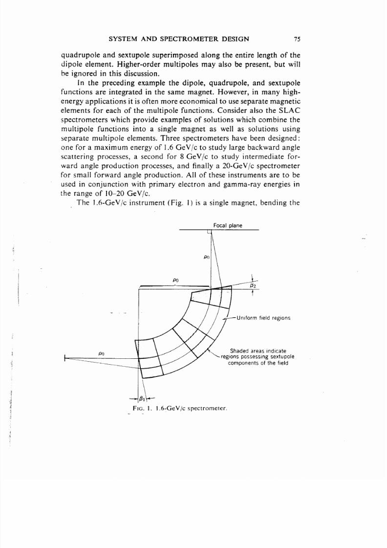
The 1.6-GeV/c instrument (Fig. 1) is a single magnet, bending the
Focal plane
Po
~ &
Uniform field regions
PoS h a d e dareas indicate
regions possessing sex tupole
\_components of the field
\
4LIFIG. 1. 1.6-GeVlc spectrometer.
-.
5/12/2018 Accel Notes - slidepdf.com
http://slidepdf.com/reader/full/accel-notes 8/66
76 K. L. BROWN
central trajectory a total of 90°, thus constituting the dipole contribution
to the optics of the system. Two quadruple elements are present in the
magnet; i.e.. input and output pole faces of the magnet are rotated so asto provide transverse focusing. and the 90° bend provides radial
focusing via the (1 – }Z)12factor characteristic of any dipole magnet.
The net optical result is point-to-point imaging in the plane of bend and
parallel-to-point imaging in the plane transverse to the plane of bend.
The solid angle and resolution requirements of the 1.6-GeV/c spectrom-
eter are such that three sextupole components are needed to achieve
the required performance. In this application, the sextupoles are
generated by machining an appropriate transverse second-order curva-
ture on the magnet pole face at three different locations along the 90°
bend of the system. In summary, the 1.6-GeV/c spectrometer consists ofone dipole, bending a total of 902, two quadruple elements, and a sex-
tupole triplet with the quadruple and sextupole strengths chosen to
provide the first- and second-order properties demanded of the system.
Momentum-measuring counter array,\
Production-angle-measuring counter array
\\ >,
>~?-.
15°Q3 ~~ “ “ I
I o
,,
o
, :;,,.
+- -gg----- “::4:’”
I
~Total path -I
w
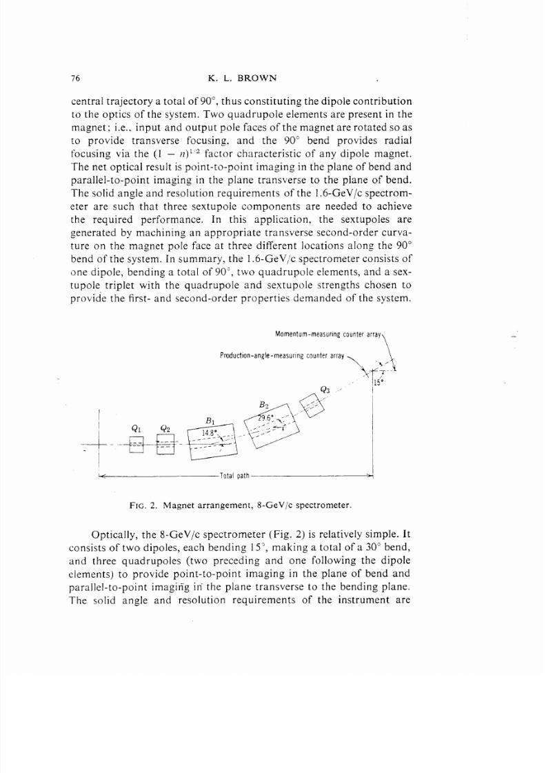
FIG. 2. Magnet arrangement, 8-GeV/c spectrometer.
Optically, the 8-GeV/c spectrometer (Fig. 2) is relatively
consists of two dipoles, each bending 159, making a total of a
simple. It
30° bend,
and three quadruples (two preceding and one following the dipole
elements) to provide point-to-point imaging in the plane of bend and
parallel-to-point imagitig ii the plane transverse to the bending plane.
The solid angle and resolution requirements of the instrument are
5/12/2018 Accel Notes - slidepdf.com
http://slidepdf.com/reader/full/accel-notes 9/66
SYSTEM AND SPECTROMETER DESIGN - 77
sufficiently modest that no sextupole components are needed. The
penalty paid for not adding sextupole components is that the focal planeangle with respect to the optic axis at the end of the system is a relatively
small angle (13.70). With the addition of one sextupole element near the
end of the system, the focal plane could have been rotated to a much
larger angle. However, the 13.7° angle was acceptable for the focal plane
counter array and as such it was ultimately decided to omit the addi-
tional sextupole element.
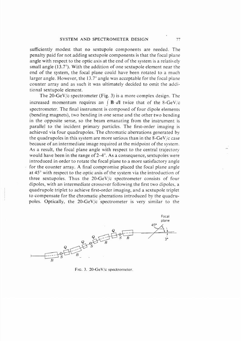
The 20-GeV/c spectrometer (Fig. 3) is a more complex design. The
increased momentum requires an f B. d] twice that of the 8-GeV’cdspectrometer. The final instrument is composed of four dipole elements
(bending magnets), two bending in one sense and the other two bendingin the opposite sense, so the beam emanating from the instrument is
parallel to the incident primary particles. The first-order imaging is
achieved via four quadruples. The chromatic aberrations generated by
the quadruples in this system are more serious than in the 8-GeV/c case
because of an intermediate image required at the midpoint of the system.
As a result, the focal plane angle with respect to the central trajectory
would have been in the range of2–4°. As a consequence, sextupoles were
introduced in order to rotate the focal plane to a more satisfactory angle
for the counter array. A final compromise placed the focal plane angle
at 45” with respect to the optic axis of the system via the introduction ofthree sextupoles. Thus the 20-GeV/c spectrometer consists of four
dipoles, with an intermediate crossover following the first two dipoles. a
quadruple triplet to achieve first-order imaging, and a sextupole triplet
to compensate for the chromatic
poles. Optically, the 20-GeV/c
aberrations introduced by the quadru-
‘spectrometer is very similar to the
Focal
plane
Q
Q
B
FIG. 3. 20-GeV/c spectronleter.

5/12/2018 Accel Notes - slidepdf.com
http://slidepdf.com/reader/full/accel-notes 10/66
78 K. L. BROWN
1.6-GeV/c spectrometer and yet physically it is radically different because
of the method of introducin& the various multipole components.
Having provided some representative examples of spectrometer
design, we now wish to introduce and develop the theoretical tools for
creating other designs.
II. A General First- and Second-Order Theory of
Beam Transport Optics
The fundamental objective is to study the trajectories described b}
charged particles in a static magnetic field. To maintain the desired
generality, only one major restriction will be imposed on the field con-
figuration: Relative to a plane that will be designated as the magnetic
midplane, the magnetic scalar potential v shall be an odd fu nction in th e
transverse coordinate ~’(the direction perpendicular to the midplane),
i.e., P(.Y,}’, ?) = –v(.Y, –j’, t). This restriction greatly simplifies the
calculations, and from experience in designing beam transport systems
it appears that for most applications there is little, if any, advantage to
be gained from a more complicated field pattern. The trajectories ~~ill
be described by means of a Taylor’s expansion about a particular
trajectory (which lies entirely within the magnetic midplane) designated
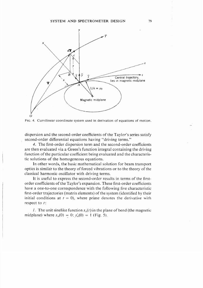
henceforth as the central trajectory. Referring to Figure 4, the coordinate
I is the arc length _measured along the central trajectory; and ,~>~’Iand 1
form a right-handed curvilinear coordinate system. The results will be
valid for describing trajectories lying close to and making small angles
with the central trajectory.
The basic steps in formulating the solution to the problem are as
follows :
1. A general vector differential equation is derived describing thetrajectory of a charged particle in an arbitrary static magnetic field
which possesses “midplane symmetry. ”
2. A Taylor’s series solution about the central trajectory is then
assumed; this is substituted into the general differential equation and
terms to second-order~n the initial conditions are retained.
3. The first-order coefficients of the Taylor’s expansion (for mono-
energetic rays) satisfy homogeneous second-order differential equations
characteristic of simple harmonic oscillator theory: and the first-order
5/12/2018 Accel Notes - slidepdf.com
http://slidepdf.com/reader/full/accel-notes 11/66
SYSTEM AND SPECTROMETER
Y
DESIGN 79
/~
7’
Y
B ~, (; ~ tCentral trajectory,
x
Tlies In magnetic midplane
A
I/h = po
o
FIG. 4. Curvilinear coordinate system used in derivation of equations of motion.
dispersion and the second-order coefficients of the Taylor’s series satisfy
second-order differential equations having “driving terms. ”
4. The first-order dispersion term and the second-order coefficientsare then evaluated via a Green’s function integral containing the driving
function of the particular coefficient being evaluated and the characteris-
tic solutions of the homogeneous equations.
In other words, the basic mathematical solution for beam transport
optics is simila-r to the theory of forced vibrations or to the theory of the
classical harmonic oscillator with driving terms.
It is useful to express the second-order results in terms of the first-
order coefficients of the Taylor’s expansion. These first-order coefficients
have a one-to-one correspondence with the following five characteristic
first-order trajectories (matrix elements) of the system (identified by theirinitial conditions at t = 0), where prime denotes the derivative with
respect to t:
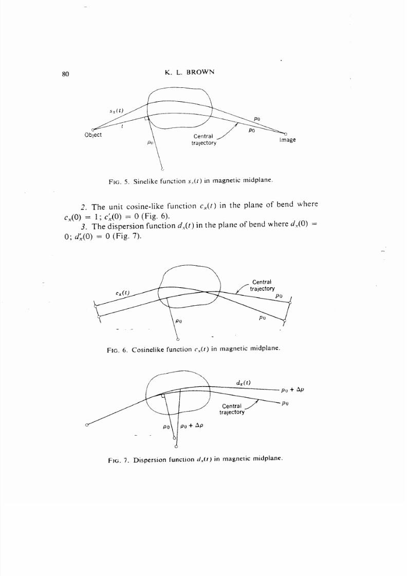
1. The unit sinelike function SX(t)in the plane of bend (the magnetic
midplane) where SX(0) ~ O;-S~(0) = 1 (Fig. 5).
5/12/2018 Accel Notes - slidepdf.com
http://slidepdf.com/reader/full/accel-notes 12/66
80 K. L. BROWN
S.r(t)
Object
P() t ra jec to ryImage
FIG. 5. Sinelike function s,(f) in magnetic midplane.
2. The unit cosine-like function CX([) in the plane of bend where
c.(O) = l;c~(0) = O(Fig. 6).
3. Thedispersion function dY(r)int heplaneo fbendwhered.~(O) =
O;d~(0) =O(Fig. 7).
\
FIG. 6. Cosinelike function {’.T(1)in magnetic midplane.
p. + AP
Pu
-.
Fl~, 7. Dispersion funclion fi..(f) in magnelic midplane.

5/12/2018 Accel Notes - slidepdf.com
http://slidepdf.com/reader/full/accel-notes 13/66
SYSTEM AND SPECTROMETER DESIGN 81
4. The unit sinelike function SV(t) in the nonbend plane where
s,(O) = O; s;(O) = 1 (Fig. 8).
Y Diane
Sy (t)
—t
Object
m’
Image
FIG. 8. Sinelike function s,(r) in nonbend (y) plane.
5. The unit cosinelike function eV(t) in the nonbend plane where
CV(0)= 1 ; c;(O) = O (Fig. 9).
j Writing the first-order Taylor’s expansion for the transverse position of
i an arbitrary trajectory at position t in terms of its initial conditions, the
~- above five quantities are just the coefficients appearing in the expansion
i for the transverse coordinates x and y as follows:i‘ii x(t) = cX (t)xO + sX (t )x~ + dX(t)(Ap/ pO)
i and
1 y(t)= C.(t)yo + S.(t)y:
;
where X. and y. are the initial transverse coordinates and x: and ,v: are
the initial angles (in the paraxial approximation) the arbitrary ray makes
‘uFIG. 9. Cosinelike function c,(t) in nonbend (y) plane.

5/12/2018 Accel Notes - slidepdf.com
http://slidepdf.com/reader/full/accel-notes 14/66
82
with respect to the central
deviation of the ray from
K. L. BROWN
trajectory. Ap/pO is the fractional momentum
the central trajectory.
1. TIIe Vector D[~erential Equalion of Mot ion
We begin with the usual vector relativistic equation of motion for a
charged particle in a static magnetic field equating the time rate of
change of the momentum to the Lorentz force:
P=e(Vx B)
and immediately transform this equation to one in which time has been
eliminated as a variable and we are left only with spatial coordinates.The curvilinear coordinate system used is shown in Figure 4. Note that
the variable t is not time but is the arc distance measured along the
central trajectory. With a little algebra, the equation of motion is
readily transformed to the following vector forms shown below:
Let e be the charge of the particle, V its speed, P its momentum
magnitude, T its position vector, and T the distance traversed. The unit
tangent vector of the trajectory is dT/dT. Thus, the velocity and momen-
tum of the particle are, respectively, (dT/dT) V and (dT/dT)P. The
vector equation of motion then becomes:
‘$(:p)=ev($x)or
- Pd2Tm+#(#)=e(#xB)
where B is the magnetic induction. Then, since the derivative of a unit
vector is perpendicular to the unit vector, d2T/dT2 is perpendicular to
dT/dT. It follows that dP/dT = O; that is, P is a constant of the motion
as expected from the fact that the magnetic force is always perpendicular
to the velocity in a static magnetic field. The final result is:
(1)
2. The Coordinate S~tem
The general right-handed
used is illustrated in Figure 4.
curvilinear coordinate system (x, y, t)
A point 0 on the central trajectory is

5/12/2018 Accel Notes - slidepdf.com
http://slidepdf.com/reader/full/accel-notes 15/66
SYSTEM AND SPECTROMETER DESIGN 83
designated the origin. The direction of motion of particles on the central
trajectory is designated the positive direction of the coordinate ~. A
point A on the central trajectory is specified by the arc length t measured
along that curve from the origin O to point A. The two sides of the
magnetic symmetry-plane are designated the positive and negative sides
by the sign of the coordinate ~’.To specify an arbitrary point B which
lies in the symmetry plane, we construct a line segment from that point
to the central trajectory (which also lies in the symmetry plane) inter-
secting the latter perpendicularly at A : the point .4 provides one
coordinate t: the second coordinate -r is the length of the line segment
BA, combined with a sign (+) or (–) according as an observer, on thepositive side of the symmetry-plane, facing in the positive direction of
the central trajectory, finds the point on-the left or right side. In other
\vords, .Y,~’, and t form a right-handed curvilinear coordinate system.
To specify a point C \\hich lies off the symmetry-plane, we construct a
line segment from the point to the plane. intersecting the latter per-
pendicularly at B: then B provides the t~vo coordinates, t and Y: the
third coordinate ~ is the length of the line segment CB.
L;’e now define three mutually perpendicular unit vectors (f, j, i).
f is tangent to the central trajectory and directed in the positive t-
direction at the point A corresponding to the coordinatet;.i
is perpen-dicular to the principal trajectory at the same point, parallel to the
symmetry plane, and directed in the positive .Ydirection. O is perpen-
ciicular to the symmetry plane, arid directed away from that plane on its
posi[ile side. -The unit vectors (i, j, f) constitute a right-handed system
and satisfy the relations
The coordinate t is the primary independent variable, and we shall
use the prime to indicate the operation (f/dt.The unit vectors depend
only on the coordinate t, and from differential vector calculus, we may
write
.t’ = 171
j’=o
i’ = –11.c (3)

5/12/2018 Accel Notes - slidepdf.com
http://slidepdf.com/reader/full/accel-notes 16/66
84 K. L. BROWN
where /~([) = I/pO is the curvature of the central trajectory at point A
defined appositive as shown in Figure4.The equation of motion may now be rewritten in terms of the
curvilinear coordinates defined above. To facilitate this, it is convenient
to express dT/dT and dcT/dTQ in the following forms:
The equation of motion now takes the form
(4)
In this coordinate system, the differential line element is given by:
Differentiating these equations with respect to t,it follows that:—
T’z = .Y’Q+ j’2 + (1 +- i~x)~
1 d- – T’ 2 = x’x” + ~“j’” + (i + /Ix)(~Ix’ + ~7’X)2dt( )
T’ = .fx’ + j]” + (1 + hX)f
and
T“ = .fx” + .f’x’ + jy”+ j’}’ + (] + i?.v)t’ + f(/?X’ + //’x)
Using the differential vector relations of Eq. (3), the expression for T“
reduces to -.
T“ = .f[X” – / ~(1 + 17.Y)] + -jj” + i[2/~.Y’+ /1’.Y]
5/12/2018 Accel Notes - slidepdf.com
http://slidepdf.com/reader/full/accel-notes 17/66
SYSTEM AND SPECTROMETER DESIGN - 85
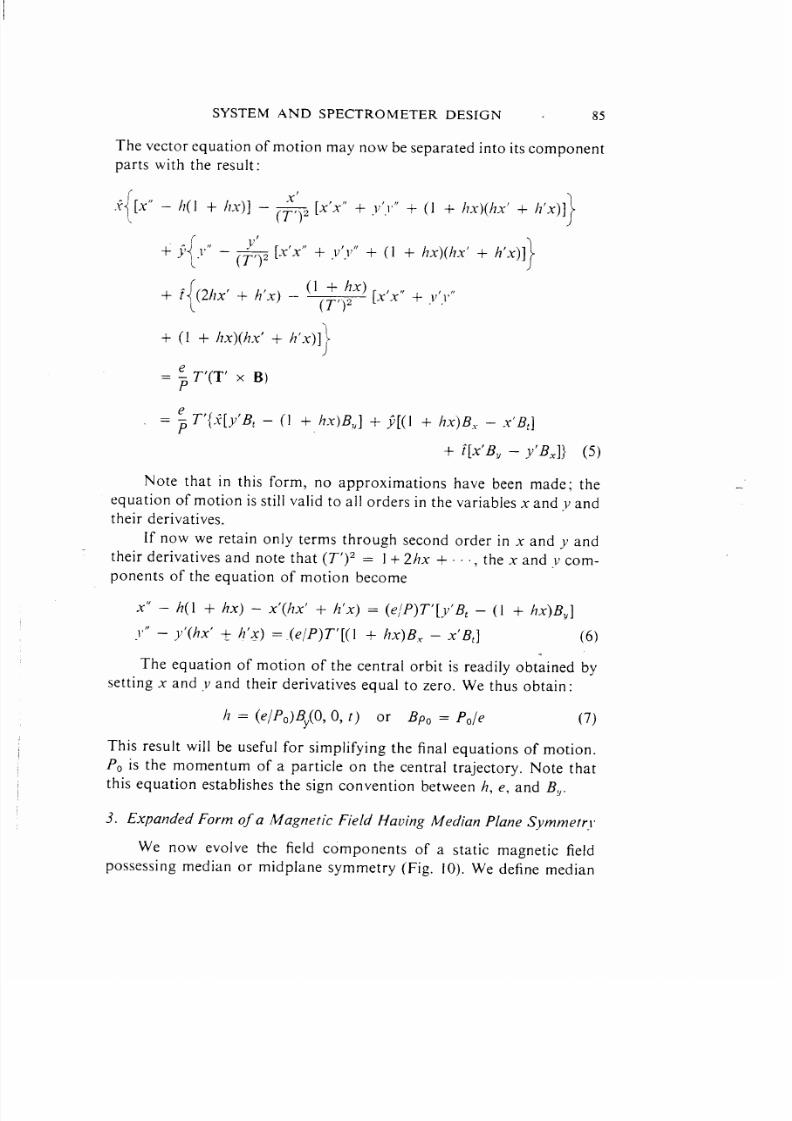
The vector equation of motion may now be separated into its component
parts with the result:
{.f [x” –
+
+
+
—
—
A(1 + hx)] – ~(~’)2 [x’x” + ~)’,,,
+ (1 + I?x)(hx’ + /?’x)]}
{
I
j j,” – - y’x” + .V ’j)” + ( I + Ax)(hx’ + ~’x)]~;,),[- ){(2hx’ + h’x) – (’(;,;X) [x’x” + JJ’j”
(1 + hx)(hxf + h’x)])
~ T’(T’ X B)
; T’{.t[y’B, – (1 + A.Y)B,] + j[(l + AX)B.Y– .Y’B:]
+ f[x’Bv – y’Bx]} (5)
Note that in this form, no approximations have been made; the
equation of motion is still valid to all orders in the variables x and .Yand
their derivatives.
If now we retain only terms through second order in x and y and
their derivatives and note that (T’)z = 1+ 2hx + ~, the x and v com-
p o n e n t s o f t h e e q u a t i o n o f mo t i o n become
x “ – h(l + hx) – x’(hx’ + h’x) = (e/P) T’[y’B, – (1 + hx)BV]
j’” — y’(hx’ ~ /?’x) = _(e/P)T’[( I + hx)BY – x’B,] (6)
The equation of motion of the central orbit is readily obtained by
setting x and v and their derivatives equal to zero. We thus obtain:
h = (e/PO) BY(O,O, t) or BPO = PO/e (7)
This result will be useful for simplifying the final equations of motion.
PO is the momentum of a particle on the central trajectory. Note that
this equation establishes the sign convention between h, e, and Bv.
3. Expanded Form of a Magnetic Field Having Median Plane Symmetr!
We now evolve the field components of a static magnetic field
possessing median or midplane symmetry (Fig. 10). We define median

5/12/2018 Accel Notes - slidepdf.com
http://slidepdf.com/reader/full/accel-notes 18/66
86 K. L. BROWN
Dipole Quadruple Sextupole
FTG. 10. illustration of magnetic rnidplane for dipole, quadruple, and sextupole
elements. The magnet polarities may. of course, be reversed.
plane symmetry as follows. Relative to the plane containing the central
trajectory, the magnetic scalar potential q is an odd function in ~’; i.e.,
~(.Y,j’, r) = – V(.Y,–~, t). Stated in terms of the magnetic field com-
ponents B.,. Bu, and B!, this is equivalent tO saYing that:
B,(x, y, f) = B.(x, –j), f)a n d
Bt(.Y, y, f ) = – Bt(.Y, –y, t )
It follows immed~ately that on the midplane B. = Bt = Oand only Bu
remains nonzero; in other words, on the midplane B is always normal
to the plane. As such, any trajectory initially lying in the midplane will
remain in the midplane throughout the system.
The expanded form ofa magnetic field with median plane symmetry
has been worked out by many people; however, a convenient and com-
prehensible reference is not always available. L. C. Teng(2) has providedus with such a reference.
For the magnetic field in vacuum, the field may be expressed in
terms of a scalar potential v by B = Vq. * The scalar potential will be
expanded in the curvilinear coordinates about the central trajectory
* For convenience, wc omit the minus sign since we are restricting the problem
to static magnetic fields.

5/12/2018 Accel Notes - slidepdf.com
http://slidepdf.com/reader/full/accel-notes 19/66
SYSTEM .4ND SPECTROMETER DESIGN S7
lying in the median plane ~, = O. The curvilinear coordinates have been
defined in Figure 1 where x is the outward normal distance in themedian plane away from the central trajectory. y is the perpendicular
distance from the median plane, f is the distance along the central
trajectory, and h = h(t) is the curvature of the central trajectory. As
stated previously, these coordinates (x, ~~,and t) form a right-handed
orthogonal curvilinear coordinate system.
As has been stated, the existence of the median plane requires that
~ be an odd function of ~’, i.e., ~(x, ~, /) = –p(x, –y, t). The most
general expanded form of ~ may, therefore, be expressed as follows:
(8)
where the coefficients AQ~+~. are functions of t.
[ n this coordinate system, the differential line element dTis given by
dT2 = dx2 + dy2 + (1 + hx)2(dt)2 (9)
The Laplace equation has the form
Vzp =1-
(1 + hx) & [(1 + hx)~
1— 22q la+— ——
[In
Zy 1+(l+hx)at (l+hx)~ ‘o flo)
Substitution of Eq. (8) into Eq. (10) gives the following recursion formula
for the coefficients:
+ 3nhA2m+3,. -1 +
where prime means
A with one or more
3n(n–l)h2A2~+3,n_2
+ n(n – I)(n – 2)h3A2m+3,n-3 (1 ])
d/dt, and where it is understood that all coefficients
negative subscripts are zero. This recursion formula

5/12/2018 Accel Notes - slidepdf.com
http://slidepdf.com/reader/full/accel-notes 20/66
88 K. L. BROWN
expresses all the coefficients in terms of the midplane field B,(x, O, t):
where8“BY
()A—.n = – functions oft (12)
dxn ~=oV=o
Since p is an odd function ofy, on the median plane we have B.. = Bt =
O. The normal (in x direction) derivatives of BU on the reference curve
defines BUover the entire median plane, hence the magnetic field B over
the whole space. The components of the field are expressed in terms of
p explicitly by B = Vp or
where Bt is not expressed in a pure power expansion form. This form can
“be obtained straightforwardly by expanding 1/(1 + hx) in a power series
of Ax and multiplying out the two series; however, there does not seem
to be any advantage gained over the form given in Eq. (13).
The coefficients up to the sixth-degree terms in x and y are given
explicitly below from Eq. (1 1).
h’A~o – Ala – hA12 + h2A11
2h’A; l – 6h2A; o – 6hh’A;o – A14
– hA,3 + 2h2A12 – 2h3A,,
3h’A;, – 18h2A;1 – 18hh’A; l
+ 36h2h’A;o – Als – hA14 + 3h2A13— 6h3A,2 + 6h4A11 (14)
A 50 = A~o + 2A~2 – 2hA:1 + h“A1l + 4h2A~o + 5hh’Aj0
-. + A14 + 2hA13 – h2A12 + h3All
A A~l – 4hA~o – 6h’A% – 4h’’A;o – 11’’’A;o+ 2A;31 =— 6hA:2 – 2h’Ai2 + h“A1z + 10h2A;l + 7h h’A; l – 411 z’’A11
– 3h’2A11 – 16h3A~o – 29h2h ’A~o + A1~ + 211A14
— 3h2A10 + 3h3A, z – 3h4A11 (15)

5/12/2018 Accel Notes - slidepdf.com
http://slidepdf.com/reader/full/accel-notes 21/66
SYSTEM AND SPECTROMETER DESIGN 89
In the special case when the field has cylindrical symmetry about .O,we can choose a circle with radius pO = l//z = a constant for the
reference curve. The coefficients A~m+ l,n in Eq. (8) and the curvature }1
of the reference curve are then all independent of t.Eqs. (14) and (15)
are greatly simplified by putting all terms with primed quantities equal
to zero.
4. Field Expansion to Second Order Only
If the field expansion is terminated with the second-order terms, the
results may be considerably simplified. For this case, the scalar potential
q and the field B = VT become:
A3nBU
ln=—ax’
= functions oft only~=oY=o
and
A 30 = –[A;o + hA1l + Al,]
where prime means the total derivative with respect to t.Then B = V9
from which
Bt(x, y> t) =1-
(1 + hx): = (1 ;hx)[A~oy + ‘; ’xy ‘“’l (16J
By inspection it is evident that Bx, By, and Bt are all expressed in terms
of Ale, All, and Alz and their derivatives with respect tot.
Considerthen BV on the midplane only
BY(x, 0, t) = AIO + Allx + ~A12x2 + . .
dipole - quadruple sextupole etc.
(17)
5/12/2018 Accel Notes - slidepdf.com
http://slidepdf.com/reader/full/accel-notes 22/66
90 K. L. BROWN
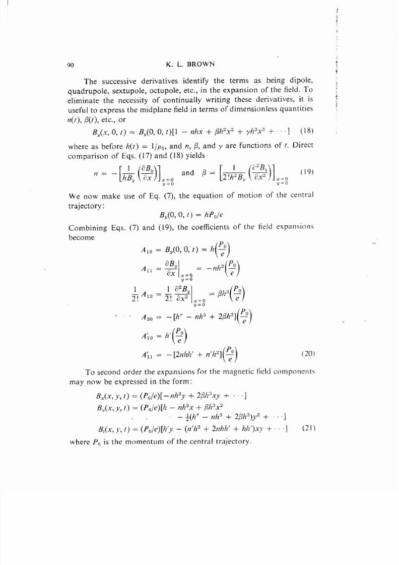
The successive derivatives identify the terms as being dipole,
quadruple, sextupole, octupole, etc., in the expansion of the field. Toeliminate the necessity of continually writing these derivatives, it is
useful to express the midplane field in terms of dimensionless quantities
n(t), ~(t), etc., or
BY(X,o, f) = BY(O, o, t)[l – Mhx + ph2x2 + yh3x3 + ] (18)
where as before h(t) = I/pO, and n, ~, and y are functions of t. Direct
comparison of Eqs. (17) and (18) yields
We now make use of Eq. (7), the equation of motion of the central
trajectory:
BY(O, o, t) = hPo/ e
Combining Eqs. (7) and (19), the coefficients of the field expansions
become
1 ~2BY+, A,2=– — ,=0 = ph3(:)
2! 8X2 ~=o
();l = – [2nhh’ + )?’h2] : (20)
To second order the expansions for the magnetic field components
may now be expressed in the form:
BX(X,y, t) = (Po/ e)[– n h2y + 2~h3xy + ~]
B,,(x, y, t) = (Po/ e)[h – 17/72x+ ~h3x2
-. – +(h” – nh3 + 2~h3)y2 + ~~]
B,(x, j’, t) = (PO/ e)[h ’y – (~’h2 + 2iIhh’ + hh’)x~ + ] (21)
where P. is the momentum of the central trajectory

5/12/2018 Accel Notes - slidepdf.com
http://slidepdf.com/reader/full/accel-notes 23/66
SYSTEM AND SPECTROMETER DESIGN 91
5. Identlycation of n and ~ }~itll Pure Quadruple and Sextupole Fields
The scalar potential of a pure quadruple field in cylindrical and in
rectangular coordinates is given by:
T = (BOr2/ 2a)sin 2a = BOx~’/a (2~~)
where BO is the field at the pole, a is the radius of the quadruple aperture
and r and a are the cylindrical coordinates, such that x = r cos a and
y = r sin a. From B = VP, itfollows that
BX = BOy/a and By = BOx/a (2~b)
Using the second of Eqs. (20) and Eqs. (22a) and (22 b).
?BV BO P.=— =
()]lJ12—
ax ~=o a ey=o
where now we define the quantity kf as follows:
k: = – }tJ?2= (Bo/a)(e/Po) = (Bo/a)(l /Bp) (23)
Similarly for a pure sextupole field,
~ = (Bor3/3a2) sin 3a = (Bo/3a2)[3x2y – y3]
(24)
where B. is the field at the pole and a is the radius of the sextupole
aperture.
Using the third-pati of Eqs. (20) and Eqs. (24)
where we now define the quantity k: as follows:
k: = ~J/3 = (Bo/a2)(e/PO) = (Bo/a2)( 1/Bp) (25)
These identities, Eqs. (23) and (25), are useful in the deri~ ation of the
equations of motion and the matrix elements for pure quadruple and
sextupole fields.
6. Tllc Equal io}ls of A!oti6n iti Tllcir Fi}lal Fornl to Secojld OrdiIr
Having derived Eq. (21), we are no\v in a position t(>sljbstitllte int{}
the general second-order equations of motion. Eq. (6). Combining

5/12/2018 Accel Notes - slidepdf.com
http://slidepdf.com/reader/full/accel-notes 24/66
I$$
~
.,
,:
f
92 K. L. BROWN /
:
Eq. (6) (the equation of motion) with the expanded field components of ‘?Eq. (21), we find for x
i
x“ — h(l + Ax) – X’(hx’ + h’x)
= (pO/p)T’{(l + hX)[- h + nh2x – ~h3x2 + ~(h” – r?iz3+ 2~h3)J2]
+ /r’j’j” + ‘}
and for y
j’” — y’(hx’ + h’x)
= (pO/P)T’{ – X’h’y – (1 + hx)[l?h2j – 2ph3xJ’] + [
Note that we have eliminated the charge of the particle e in the equations
of motion. This has resulted from the use of the equation of motion of
the central trajectory.
Inserting a second-order expansion for T’ = (Y” +
(1 + hx)2)1’2 and letting
we finally express the differential equations for .Yand J to second
as follows:
x“ + (1 — )?)h2x = }18 + (2/? – 1 – p)h3x2 + il’xx’ + +hx’2
+ (2 – ~)h2X8 + ~(h” – ??h3+ 2~h3)y2 + h’},~’ – ~h~,’2–
+ higher-order terms
)’” + llh2Y = 2(8 : /?]h3XY+ h’X~’ – h’X’J’ + h.~’]’ + / lh2}’8
+ higher-order terms
1“’2+
(26)
order
h82
(27)
(~s)
From Eqs. (27) and (2S) the familiar equations of motion for the
first-order terms may be extracted:
X“ + (1 – Il)h2.x = 116 and ~“ + )lhz)’ = O (29)
Substituting k: = –}lh2 from Eq. (23) into Eqs. (27) and (28). the
second-order equations of motion for a pure quadruple field result b}
taking the timit h -0, h’ ~ O and h“ –~ O. We find that
.YJ+ k;x = k:xs
l’” —k:)’ = – k:J’8
where
k: = (BO/a)(e/PO) = (Bo/a)( 1/Bpo) (30)
5/12/2018 Accel Notes - slidepdf.com
http://slidepdf.com/reader/full/accel-notes 25/66
SYSTEM AND SPECTROMETER DESIGN 93
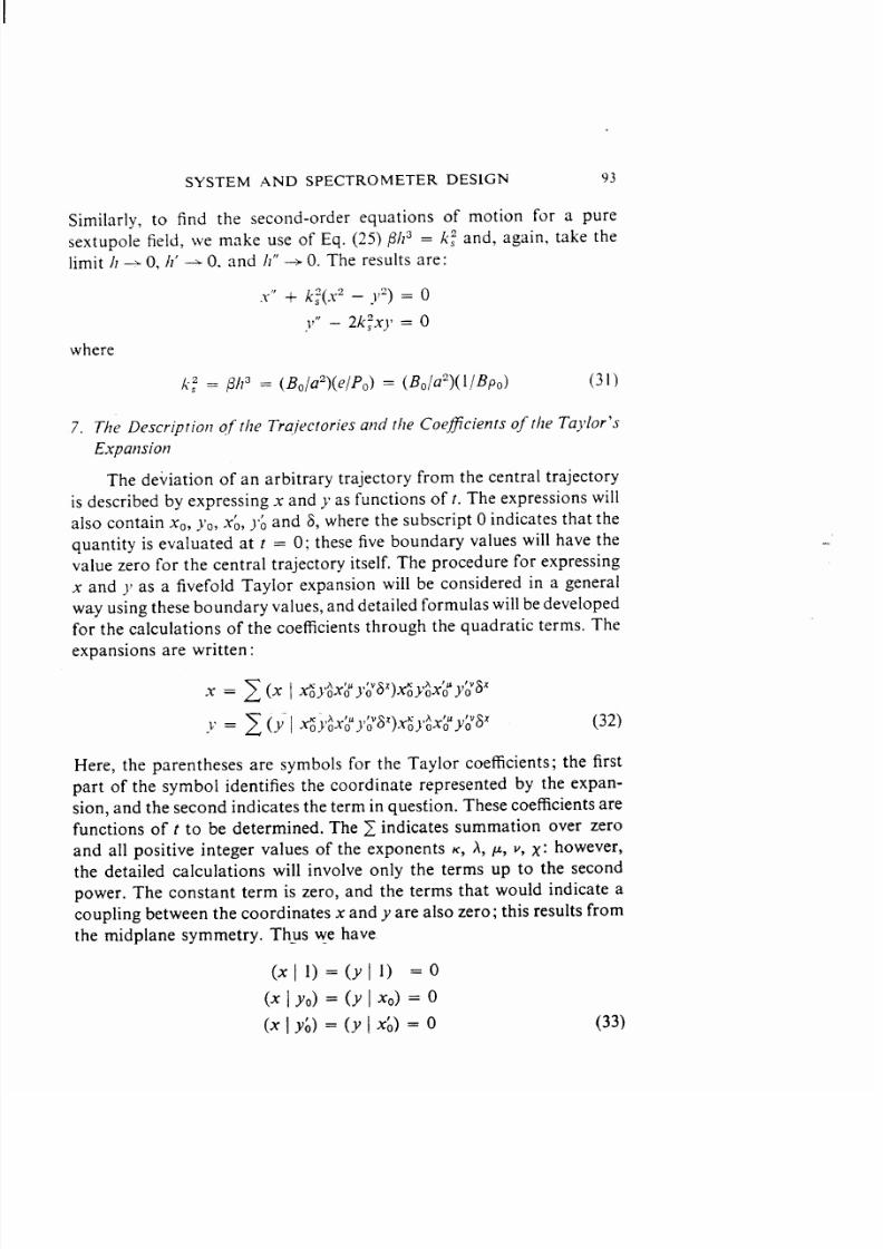
Similarly, to find the second-order equations of motion for a pure
sextupole field, we make use of Eq. (25) ~~13= k: and, again, take the
limit /1-O, 11’-0. and II” ~ O. The results are:
.Y”+ k:(x2– J’z)= o
~?”— 2k:x)’ = o
where
k: = p/73 = (Bo/a2)(e/Po) = (Bo/a2)(l~Po) (31)
7. T}le Description of tile Trajectories and t}le Coe@cients of t}le Ta}’lor ’s
Expansion
The deviation of an arbitrary trajectory from the central trajectory
is described by expressing x and y as functions of t.The expressions will
also contain xO,YO,xL, j’j and ~, where the SUbSCriPtOindicates that the
quantity is evaluated at r = O; these five boundary values will have the
value zero for the central trajectory itself. The procedure for expressing
x and j’ as a fivefold Taylor expansion will be considered in a general
way using these boundary values, and detailed formulas will be developed
for the calculations of the coefficients through the quadratic terms. Theexpansions are written:
Here, the parentheses are symbols for the Taylor coefficients; the first
part of the symbol identifies the coordinate represented by the expan-
sion, and the second indicates the term in question. These coefficients are
functions of t to be determined. The ~ indicates summation over zero
and all positive integer values of the exponents K, ~, W , v , x: however,
the detailed calculations will involve only the terms up to the second
power. The constant term is zero, and the terms that would indicate a
coupling between the coordinates x and y are also zero; this results from
the midplane symmetry. Thus we have.
(Xll)=(yll) = 0
(xl Yo)=(Yl~o)=o
(~16)=(Ylxb)=o (33)

5/12/2018 Accel Notes - slidepdf.com
http://slidepdf.com/reader/full/accel-notes 26/66
94 K. L. BROWN
Here, the first line is a consequence of choosing x~ = JO = O, while the,;!
isecond and third lines follow directly from considerations of symmetry. 1
or, more formally, from the formulas at the end of this section.~
As mentioned in the introduction, it is con~enient to introduce the ~fottowing abbreviations for the first-order Ta}lor coefficients:
,>,;..
( x I .Y~) = C. y ( f ) ( x I -Y:)= S .,,(?) (.Y \ 8) = d(t)‘,:
%
(J’ I yo) = cv(~) (j’ Iy~)= s.(r) (34) ,
Retaining terms to second order and using Eqs. (33) and (34), the
Taylor’s expansions of Eq. (32) reduce to the following terms:
c,. Sy d,
.Y = (x I X,)XO + (x I xj).Y: + (.Y] 8)6
+ (.Y\ X:)X8 + (.YI .Y~.Y:).Yo.Y: (.YI .Y08).Y03
+(x / x:2).Y~ + (.YI -T:8).T:8 + (.YI 82)82
+(x I j’:)}: + (x IJ’oj”:):”o.l’: + (.YIj’;)2)j’;)2
and
Cy Su
.1 = (y [ J’o)j’o + (J’ I J’:)J’:
+(J’ \ Xoj’o)xoj”o+ (j’ I -Yoj’;).l-oj’i + (J” I ~bj’o)-t-:j’o
+(J ’ I X:j ’:).x i j ” i + (j ’ \ J os )j ’o s + (j ’ I j ’j a ).l ” b a
Substituting these expansions into Eqs. (27) and (28), we derive
(35)
a di f-
ferentiat equation for each of the first- and second-order coefficients
contained in the Taylor’s expansions for .\- and .1. When this is done. a
systematic pattern evolves, namely,
c;. + k:.c., = o C; + k:cY = O
S: + k~..$,. = O or s; + k;sv = o
q : + ~ : q . , . / : , q; + k;g!, = j; (36)
where k; = (1 —11)112nd k? = IIllz for the .Yand j motl~)ns, respec-tively. The first two of these equations represent the equations of motion
for the first-order rnonoenergetic terms S.Y,c.., s,,, and cu. That there arc
two solutions, one for c and one for s, is a manifestation of the fact
that the differential equation is second order; hence, the tl~o solutions
differ only bv the initial-conditions of the characteristics and (’functions,
5/12/2018 Accel Notes - slidepdf.com
http://slidepdf.com/reader/full/accel-notes 27/66
SYSTEM AND SPECTROMETER DESIGN 95
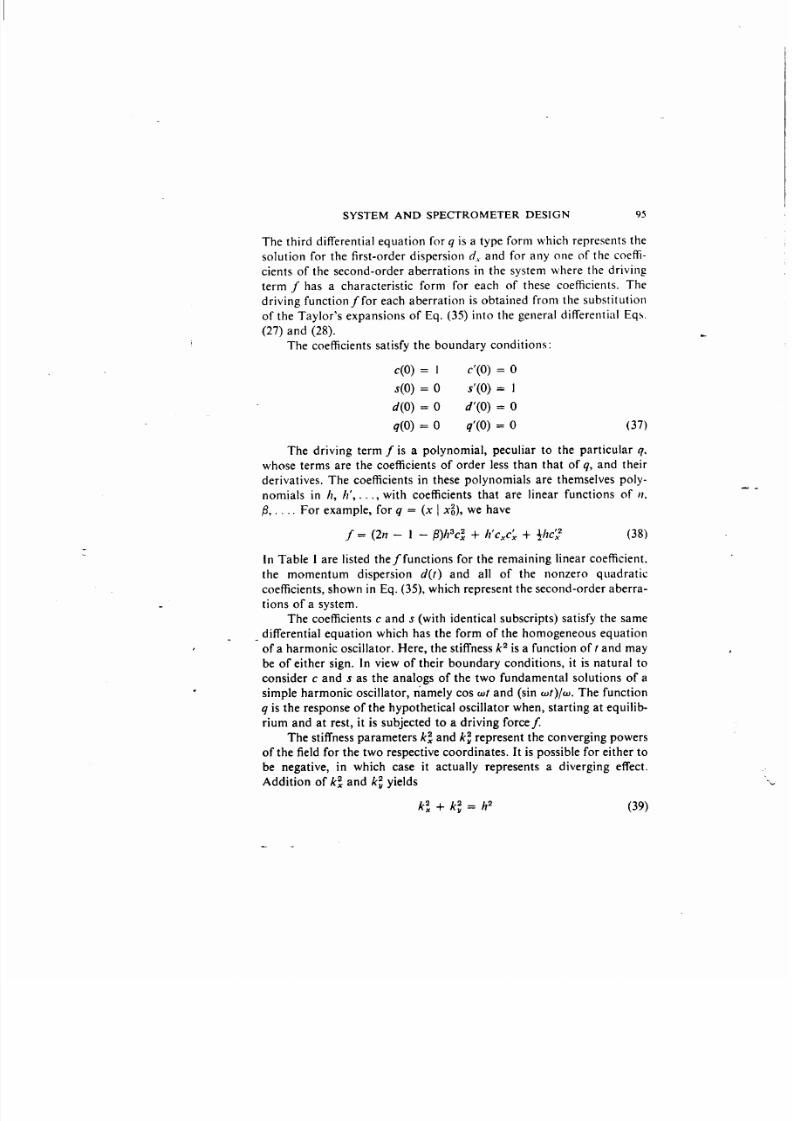
The third differential equation for q is a type form which represents the
solution for the first-order dispersion dXand for any one of the coeffi-
cients of the second-order aberrations in the system where the driving
term ~has a characteristic form for each of these coefficients. The
driving function ~for each aberration is obtained from the substitution
of the Taylor’s expansions of Eq. (35) into the general differential Eqs.
(27) and (28).
The coefficients satisfy the boundary conditions:
c(o) = I c’ (o) = os(o) = o s’(o) = 1
d(0) = O d’(0) = O
g(o) = o q’(o) = o (37)
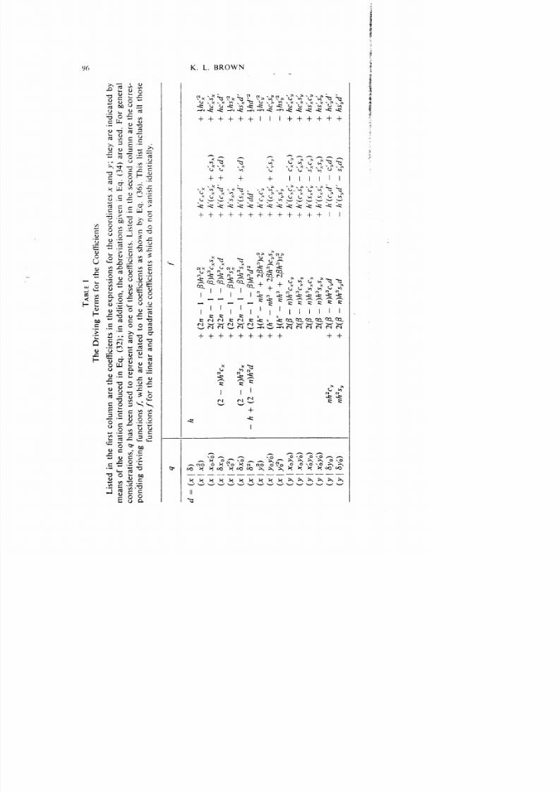
The driving term f is a polynomial, peculiar to the particular 9,
whose terms are the coefficients of order less than that of q, and their
derivatives. The coefficients in these polynomials are themselves poly-
nomials in h, h’, . . . with coefficients that are linear functions of n,
P,. For example, for g = (x I x:), we have
f=(2n- 1 – #)h3c: + /l’cXc; + +/?c:? (38)
In Table 1are listed the~functions for the remaining linear coefficient.the momentum dispersion d(r) and all of the nonzero quadratic
coefficients, shown in Eq. (35), which represent the second-order aberra-
tions of a system.
The coefficients c and s (with identical subscripts) satisfy the same
_differential equation which has the form of the homogeneous equation
of a harmonic oscillator. Here, the stiffness k2 is a function of I and may
be of either sign. In view of their boundary conditions, it is natural to
consider c and s as the analogs of the two fundamental solutions of a* simple harmonic oscillator, n’amely cos WI and (sin wf)/w. The function
q is the response of the hypothetical oscillator when, starting at equilib-
rium and at rest, it is subjected to a driving force J
The stiffness parameters k; and k: represent the converging powers
of the field for the two respective coordinates. It is possible for either tobe negative, in which case it actually represents a diverging effect.
Addition of k; and k; yields
k:+k; =h2 (39)
-.
5/12/2018 Accel Notes - slidepdf.com
http://slidepdf.com/reader/full/accel-notes 28/66
x)x)x)x)x)x)x)x)

5/12/2018 Accel Notes - slidepdf.com
http://slidepdf.com/reader/full/accel-notes 29/66
SYSTEM AND SPECTROMETER DESIGN 97
For a specific magnitude ofh, A: and k; may be varied by adjusting n, but
the total converging power is unchanged; any increase in one converging
power is at the expense of the other, The total converging power is
positive; this fact admits the possibility of double focusing.
A special case of interest is provided by the uniform field; here
h = const. and n = O; then k: = hz and k; = O. Thus, there is a
converging effect for x resulting in the familiar semicircular focusing,
which is accompanied by no convergence or divergence of y.
Another important special case is given by n = +; here, k% = k;
= h2/ 2. Thus, both coordinates experience an identical positive con-
vergence, and Cx = CUand SX= SY;that is, in the linear approximation,the two coordinates behave identically, and if the trajectory continues
through a sufficiently extended field, a double focus is produced.
The method of solution of the equations for c and s will not be
discussed here, since they are standard differential equations. The most
suitable approach to the problem must be determined in each case. In
many cases it will be a satisfactory approximation to consider h and n,
and therefore k2 also, as uniform piecewise. Then, c ands are represented
in each interval of uniformity by a sinusoidal function, a hyperbolic
function, or a linear function off, or simply a constant. Using Eq, (36),
it follows for either the x or y motions that:
; (es’ - c’s) = o
Upon integrating and using the initial conditions on c and s in Eq. (37),
we findCs’ – c’s = 1 (40)
This expression is just the determinant of the first-order transport
matrix representing either the x or y equations of motion. It can be
demonstrated that the fact that the determinant is equal to one is
equivalent to Liouville’s theorem, which states that phase areas are“
conserved throughout the system in either the x or y plane motions.
The coefficients q are evaluated using a Green’s function integral
Jq = ‘J(~)G(t, ~) d~ (41)
o
where
G(f, T) = s(f)c(T) – s(T)c(t) (42)and
J
t
J= ‘([) ~~(~)c(~) d7 – C(t) :/(T)S(T) dr (43)
--
5/12/2018 Accel Notes - slidepdf.com
http://slidepdf.com/reader/full/accel-notes 30/66
98 K, L. BROWN
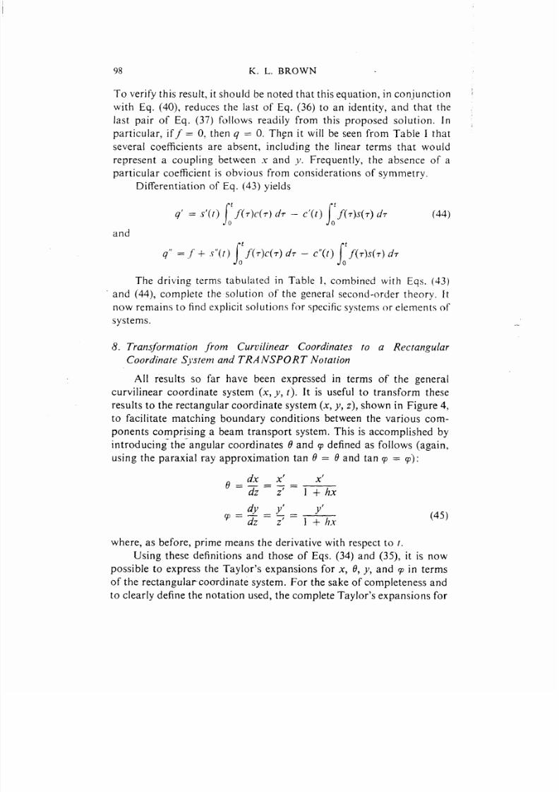
To verify this result, it should be noted that this equation, in conjunction
with Eq. (40), reduces the last of Eq. (36) to an identity, and that the
last pair of Eq. (37) follows readily from this proposed solution. In ,,
particular, if~ = O, then q = O. Th~n it will be seen from Table I thatseveral coefficients are absent, including the linear terms that would
represent a coupling between x and y. Frequently, the absence of a
particular coefficient is obvious from considerations of symmetry.
Differentiation of Eq. (43) yields
/
t
/q’ = “(f) ~f(7)~(~) ~T – c’(t) ‘f(T)~(T) dT
o
and
j
t
jq“ = ,f + $“(t) ~ f ( T ) C( T )T – c“(t) ‘ f ( T ) ~ ( T )dT
o
(44)
The driving terms tabulated in Table 1, combined with Eqs. (43)
and (44), complete the solution of the general second-order theory. It
now remains to find explicit solutions for specific systems (>relements of
systems.
8. Transformation from Curvilinear Coordinates to a R ectangu lar
Coord in ate S ystem an d TRANSPORT Notation
All results so far have been expressed in terms of the general
curvilinear coordinate system (x, y, r). It is useful to transform these
results to the rectangular coordinate system (x, y, z), shown in Figure 4,to facilitate matching boundary conditions between the various com-
ponents comprising a beam transport system. This is accomplished by
introducing-the-angular coordinates Oand p defined as follows (again,
using the paraxial ray approximation tan 0 = 8 and tan ~ = q):
dy _ y’ y’
‘=~–~=l+hx(45)
where, as before, prime means the derivative with respect to /.Using these definitions and those of Eqs. (34) and (35), it is now
possible to express the Taylor’s expansions for x, e, y, and ~ in terms
of the rectangularcomdi nate system. For the sake of completeness and
to clearly define the notation used, the complete Taylor’s expansions for

5/12/2018 Accel Notes - slidepdf.com
http://slidepdf.com/reader/full/accel-notes 31/66
SYSTEM AND SI)ECTR{)METER DESIGN 99
x, 0, Y, and ~ at the end ofa system as a function of the initial vari;~bles
are given below:
Cx x.Y (Iy~2._7
x = ( x i XO) XO + ( x I d o ) 6 0 + ( : F ) 8
+ ( x I x : ) x ; + ( x \ X o d o ) x o e o + ( x \ . Y 0 6 ) X0 8
+ ( x ] 6 ; ) 8 ; + ( x ] e ~ a ) e ~ a + ( x I 8 2 ) 8 2
+ ( x ] y : ) . v : + ( x I y o p o ) y o p ~ + ( x I q g ) q g
c ; s ; d:
e=(e+ (6
+ (6
+ ( e
Cu
x~)xo + (e I do)eo + (8x:)x: + ( eI Xoeo)xo. + (e
e:)e: + (e I e o 8 ) e o 8+ (e
Y:)Y:+ (e I Y090)Y090 + (e
Y = (Y IYO)YO + (y I qo)qo
Using the definitions of Eq (45), the coefficients appearing in Eq. (46)
may be easily related to those appearing in Eq. (35). At the same time,
we will introduce the abbreviated notation used in the Stanford
TRANSPORT Program(3) where the subscript 1 means x; 2 means e,
3 means y; 4 means 0, and 6 means 8. The subscript 5 is the path length
difference 1between an arbitrary ray and the central trajectory. Rij will
be used to signify a first-brder matrix element and Tijk will signify a

5/12/2018 Accel Notes - slidepdf.com
http://slidepdf.com/reader/full/accel-notes 32/66
Im K. L. BROWN
s e c o n d - o r d e r ma t r i x element. Thus. we may write Eq. (46) in the general
form
.Y,=
$ R,jXj(0) +~ ~Tij.Xj(”)~k(o)
)=1 j=lk=j(47)
where
. Y ~= x, X2 = 9,x3 = -v, x 4 = ~,x~=[,andx~=s
d e n o t e s t h e s u b s c r i p t n o t a t i o n .
Us i n g Eq. (45) defining d and p, the following identities among the
\ arious matrix element definitions result:
For the Taylor’s expansions for x we have:
Tlaz = (x
T 134 = (x
T 14~ = (~
For the 6 terms we have.
y~j
Y090) = (x I YoY&)
v:) = (~ IY:z) (48)

5/12/2018 Accel Notes - slidepdf.com
http://slidepdf.com/reader/full/accel-notes 33/66
SYSTEM AND SPECTROMETER DESIGN
ZGG= (o I ~z) = (X’ I 82) - A(t) d.y d:
,,, = (e] y;) = (x’ Iy:)
23, = (e I yopo) = (x’ I yoy:)
,44 = (0 I p:) = (x’ Iy:2)
For the y terms in the Taylor’s expansion:
R,, = (y I y,) = c,
R3q = (y I PO) = (y ~y:) = .Yy
313 = (Y I XOYO)
T314 = (Y I x oqo) = (y I x oj ’b) + /?(0)su
T (23 = y
324 = (Y
T -(36 — Y
346 = (Y
and finally for the q terms we have:
R4~ =(TIYO) =( Y’IYO)=:(YIYO)= c:
R 44 = (9
T -(13 — P
T -(1 4 — 9
T -(23 — q
424 = (P
T -(36 — q
446 = (9
101
(49)
(50)
All of the above terms are understood to be evaluated at the terminal
point of the system except for the quantity A(O)which is to be evaluated
at the beginning of the system. In practice, /~(0) will usually be equal to
h(~); but to retain the formalism, we show them as being different here.
All nonlisted matrix elements are equal to zero.

5/12/2018 Accel Notes - slidepdf.com
http://slidepdf.com/reader/full/accel-notes 34/66
102 K. L. BROWN
9. First- and Second-Order Matrix Fornlalism of Beanl Transport Optics ~
The solution of first-order beam transport problems using matrix :
algebra has been extensively documented. (J-6) However, it does notseem to be generally known that matrix methods may be used to solve
second- and higher-order beam transport problems. A general proof of
the validity of extending matrix algebra to include second-order terms
has been given by Brown, Belbeoch, and Bounin(7) the results of which
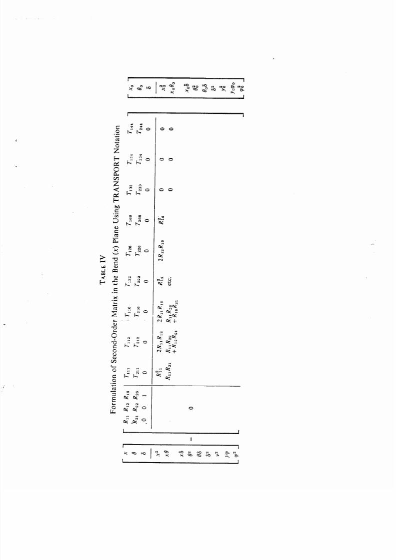
are summarized below in the notation of this report and in TRANS-
PORT notation.
Consider again Eq. (47). From ref. 3, the matrix formalism may be
logically extended to include second-order terms by extending the
definition of the column matrices xi and Xj in the first-order matrix
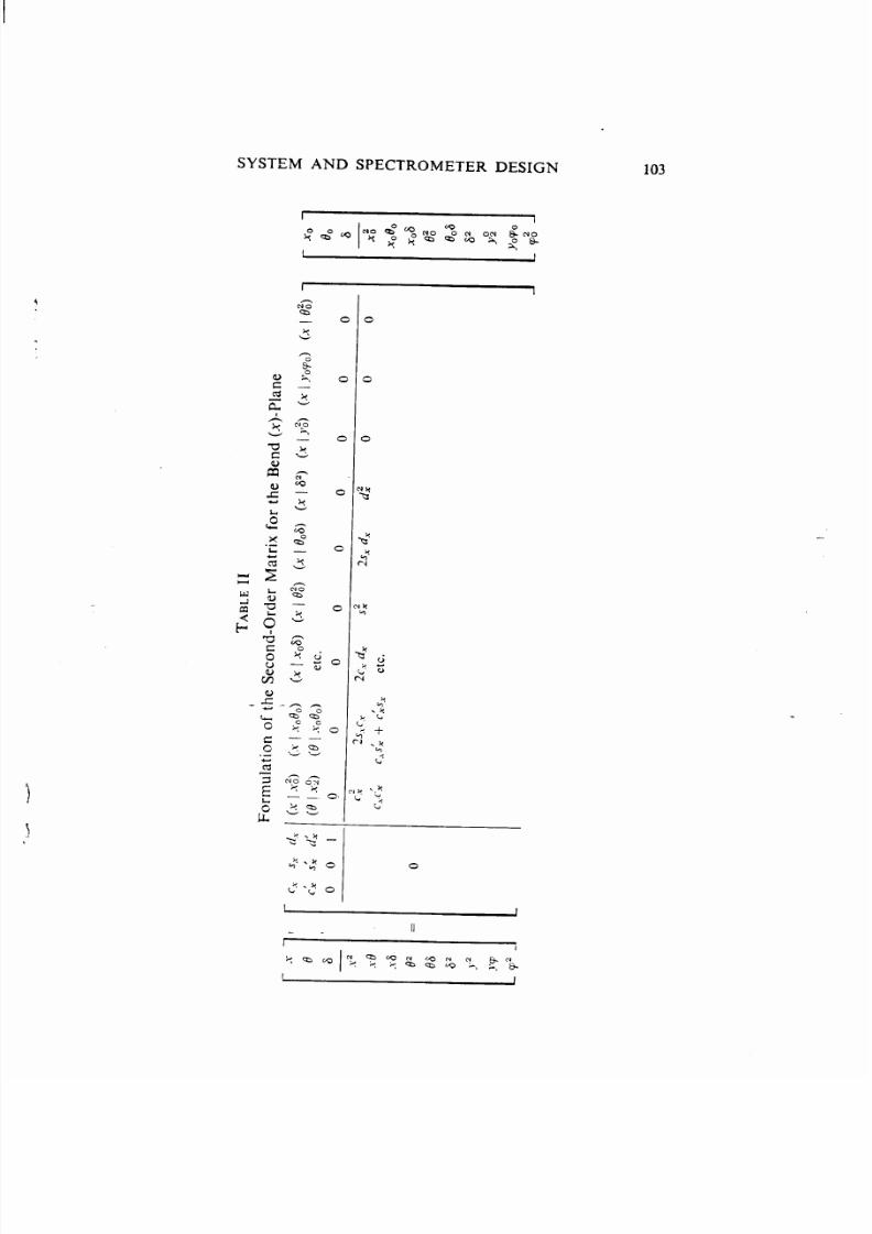
algebra to include the second-order terms as shown in Tables II–V. Inaddition, it is necessary to calculate and include the coefficients shown
in the lower right-hand portion of the square matrix such that the set of
simultaneous equations represented by Tables II–V are valid. Note that
the second-order equations, represented by the lower right-hand portion
of the matrix, are derived in a straightforward manner from the first-
order equations, represented by the upper left-hand portion of the
matrix. For example, consider the matrix in Table II; we see from row 1
that
x = CXXO+ sXOO+ dX8 + second-order terms
Hence, row 4 is derived directly by squaring the above equation as
follows: _ _
X2 = (CXXO + Sxdo + dX8)2
= C: X ;+ 2cXsXx000+ 2CXdXx08 + S ; 8 ;+ 2SXdx908 + d:82
The remaining rows are derived in a similar manner.
If now xl = ~lxO represents the complete first- and second-order
transformation from O to 1 in a beam transport system and X2 = ~zxl
is the transformation from 1 to 2, then the first- and second-order
transformation from O to 2 is simply X2 = ~2xl = MZMIXO; where Ml
and ~2 are matrices fabricated as shown in Tables 11 and 111 in our
notation or as shown in Tables IV and V in TRANSPORT notation.
5/12/2018 Accel Notes - slidepdf.com
http://slidepdf.com/reader/full/accel-notes 35/66
SYSTEM AND SPECTROMETER DESIGN103
I
f
— —
I
c
c
o
J
L I

5/12/2018 Accel Notes - slidepdf.com
http://slidepdf.com/reader/full/accel-notes 36/66
{
TBL
1
—
F
m
ao
o
th
S
Od
Max
fo
th
N
(y
Pa
c
C
Cx
SAC
S
dC
d
y
Cx
C*
S
ec
o
r
8
5/12/2018 Accel Notes - slidepdf.com
http://slidepdf.com/reader/full/accel-notes 37/66
2c.-x.-
%
: :h- h“ c
00
00
00
92Q
o

5/12/2018 Accel Notes - slidepdf.com
http://slidepdf.com/reader/full/accel-notes 38/66
o
II

5/12/2018 Accel Notes - slidepdf.com
http://slidepdf.com/reader/full/accel-notes 39/66
SYSTEM AND SPECTROMETER DESIGN 107
III. Reduction of the GeneralFirst- and Second-OrderTheory to the Case of the Ideal Magnet
Section IIofthis reportwasdevoted to thederivationof thegeneral
second-order differential equations of motion of charged particlesin a
static magnetic field, In Section 11 no restrictions were placed on the
variation of the field along the central orbit, i.e., h, n, and # were assumed
to be functions of r. As such, the final results were left in either a differen-
tial equation form or expressed in terms of an integral containing
the driving function~(t), and a Green’s function G(?, T) derived from the
first-order solutions of the homogeneous equations. We now limit the
generality of the problem by assuming h, M, and ~ to be constants over
the interval of integration. With this restriction, the solutions to the
homogeneous differential equation [Eq. (36) ~f Sec. 11]are the following
simple trigonometric functions:
Cx ( f ) COS kXr SX(?) = (l/kX) s in kxf
Cv(t) = COS k,,t s,,(I) = (]/k,,) sin kvt
where now
(52)
k: = (1 – n)h2, k; = nhz, and h = I/Po
become constants of the motion. pO is the radius of curvature of the
central trajectory. - -
The solution of the inhomogeneous differential equations [the third
of Eqs. (36)] for the remaining matrix clcmcnts is solved as indicated in
Section 11, using the Green’s functions integral Eq. (41) and the driving
functions listed in Table 1. With the restrictions that kX and k, are
constants, the Green’s functions reduce to the following simple trigono-
metric forms:
CX(t, ~) = (l/ky) sin kX(t – T)
and
G,(/UT) = (l/k,,) sin k,,(~ – T) (53)
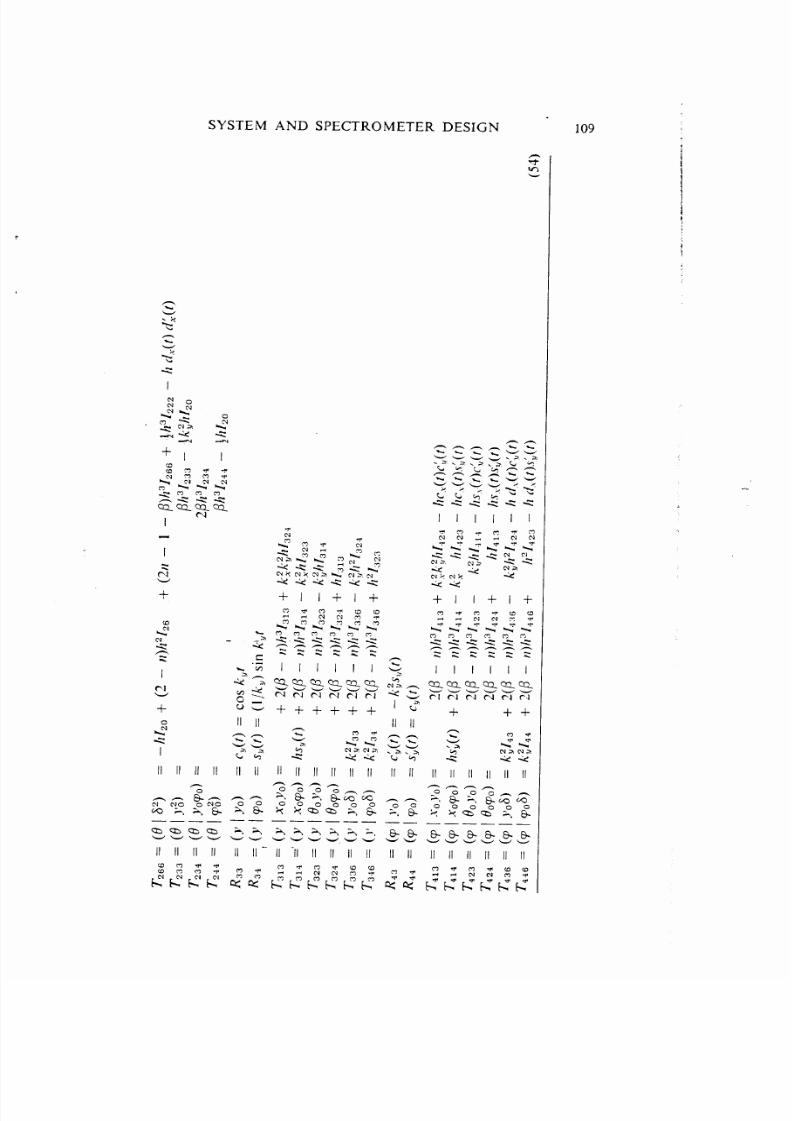
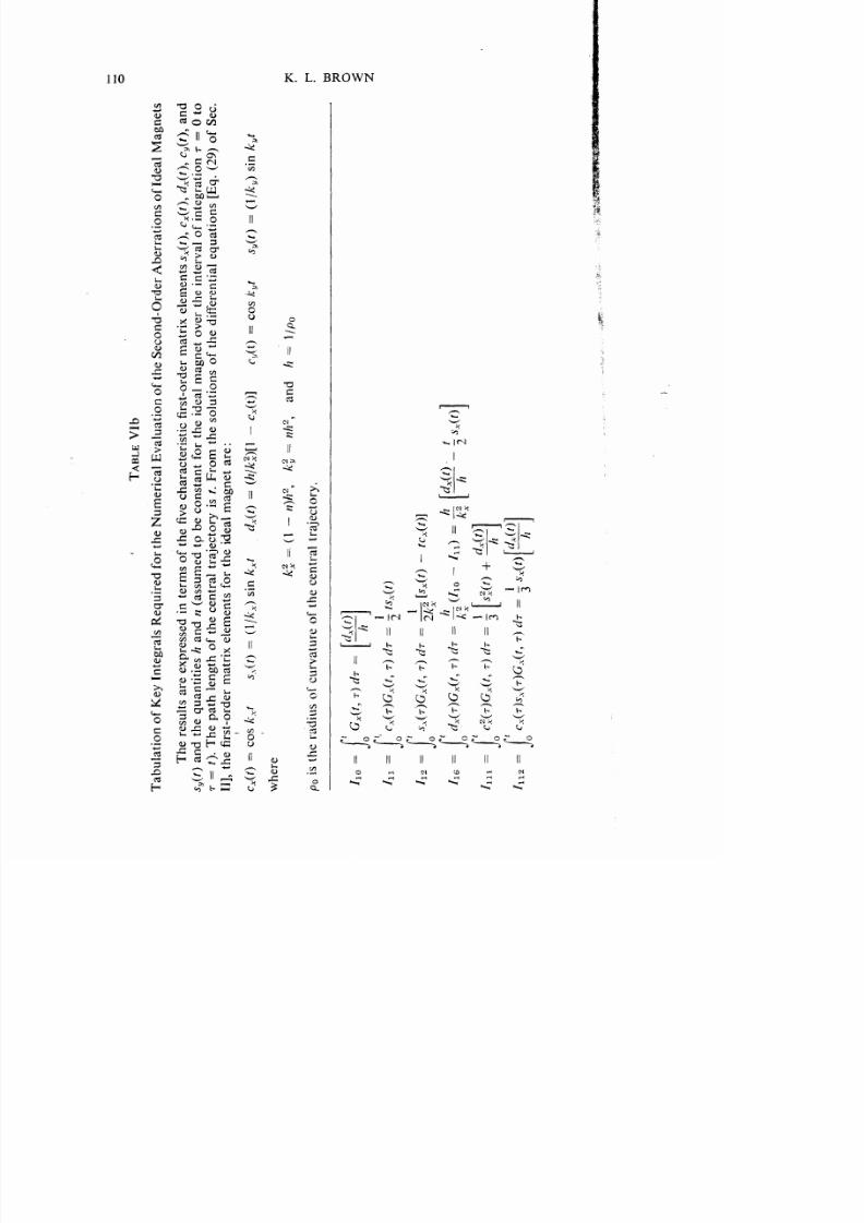
The resulting matrix elements are tabulated below in terms of the key
integrals listed in Table VI, the five characteristic first-order matrix
elements SX,CX,dX, c,, and .SYand the constants h, n , a n d P .

5/12/2018 Accel Notes - slidepdf.com
http://slidepdf.com/reader/full/accel-notes 40/66
g
TB
Va
T
ao
o
h
F
a
S
Od
Ma
x
Eem
sfoa
Id
Ma
inT
m
o
th
K
Ine
as
Lse
inT
e
Vb
R2
=
(0
T
=
(0
T
2
=
(0
T
6
=
(8
T
=
(6
T
6
=
(0
~ .
r
.Y:
=
(~1–1
_
~)h3]2,
+
+
h
_
~
2
—
1—p
.
=/
–kh
–
h
+
c~(r)sx(f)l
.Yoa)
(2/l)h2z2,+2(2)/–1–
ph
–
kh
–
h
r
~
+
c
dx(~)l
(;:)
(2/1–1–p
+~
–h
0
=
(2
–
/
h
2
2
–
1–
p
+h
–/
+s
d..(f)]
5/12/2018 Accel Notes - slidepdf.com
http://slidepdf.com/reader/full/accel-notes 41/66
SYSTEM AND SPECTROMETER DESIGN
+1
I
s+m
Ie]
+
I
—— ——a a a mww --
11 II II II
111111
11 II - II -11 II II II II II II II II II II II II
109
5/12/2018 Accel Notes - slidepdf.com
http://slidepdf.com/reader/full/accel-notes 42/66
,
TA
Vb
T
ao
o
K
Ine
as
R
e
fo
h
N
m
c
E
uo
o
h
S
Od
A
ao
o
d
Ma
s
T
reusaee
e
intem
o
h
fv
a
escf
od
m
x
eem
s
s
C
d
c
a
S
a
th
q
e
h
a
1
a
um
tp
b
c
a
fo
th
id
m
o
th
inev
o
ine
ao
7=
Oto
~=
t
T
p
h
le
h
oth
c
a
taeoy
isrFom
thso
uo
o
th
d
ee
a
e
o
[E
(2
o
S
I
th
f
od
m
x
eem
s
fo
th
id
m
ae
C
)
=
C
k
y
s(
=(
1kX
nk
~x
=
(hk
–c
c
=C
S
=(1
k
snk
w
e
k
=
(1–
t?)h2,k;=~
a
h=
IpO
p
sh
ra
u
o
c
v
ue
o
h
c
a
tae
oy
/t
1
=
[1
G
Td
=
~
oJ
t
I
=
C
T
Gx
T
d
=
;
l~
o
z
I

5/12/2018 Accel Notes - slidepdf.com
http://slidepdf.com/reader/full/accel-notes 43/66
SYSTEM AND——————..———— —---- . . . . .
111
I
+ I
.+“ I
+
- Ic l
I III

5/12/2018 Accel Notes - slidepdf.com
http://slidepdf.com/reader/full/accel-notes 44/66
\
sy(T)Gv(t,d
=
;2
[~
–
tc,(t)l
.0
-u
J
1
CyTC
TG
T
(T
=
o
~
_
4
{~
–
~v
–
2k:s..(t).Y1,(t);
2s
(t)Y
}
I

5/12/2018 Accel Notes - slidepdf.com
http://slidepdf.com/reader/full/accel-notes 45/66
[
rs~~
1
C
T~
TG
Td
=
.0
~
_
~
{2
~cY~
–
~
+
C
.
1
=
~
1
~
TC
TG
Td
=
—
{1
}
2
g
S
+
C
–
$
)~
+
~
o
k
–
4~
Jt
1
=
1
{2C
–
C
~
T~
TG
Td
=
o
k
–
4
k
}
‘Y
Y-(s}
–X)sg)=X4x
J1
=
h
[
h
t
C
T
XTG
T
T
=
—
1
–
]3
=
—
–
–
~
1
0
k
Jt
k2
k
_
4
{c
1
–
c
–
2
~
h
[
1
ISAG
1
S
TdX
TGy
Td
=
—
—
1
=
~
—
o
k
k
2k;
[s
(
–
cy(
–
1
f2
c
–
S
+
cx(~)}
k
–
4
‘
1
1=T=@
I
G
Td
=
s1
d
o
1
=
1
=~
I
~
;~
TG
T
T=~[s
+
ty
i~
=Ie=~
~
1
dto
sy(T)Gy(t,)dT=jt~y(t)~
I
/d
4
=
11
=
— d
o
C
Ts
TG
T
d
=
—
!4~
k
–2
~
~
–k
+c~
J
I
1
4
=
1
=
— d
o
C
TC
TG
T
d
=
k
_
4
{k
–
2
~
~S
–
c
–
C
1
=
I2
=
~
/
t
d
osX(TC
TG
V
T
d
=
~
_
4
{
}
2
$
c
1
+
c
–
c
–
k
+
~
x
Y
x
1
h=IZ
=~
/
1
{
x
S
TS
TG
T
d
=
[
1d
d
~
k
–
4
.
–C
y
–
2
~
1
=
Ig
=
~
/
t
[
c
T
~x
T
G
T
d
=$
jc
+S
1
d
o
k
(
+
c
–
(k
–
2
SX(c
~+
–
~
d
1
I
;
i
4
=
I4
=
—
1
.$
T
dxT
G
T
(T
=
—
—
–
d
o
_
~
{k
-
Z
Y
$
-
C
-
Cx}
~~
~
,
1
.
5/12/2018 Accel Notes - slidepdf.com
http://slidepdf.com/reader/full/accel-notes 46/66
114 K. L. BRO\VN
The constants }Z~nd ~ are defined by the midplane field expansion
[Eq. (18) of Sec. 11]:
or, from Eq. (19) of Section 11:
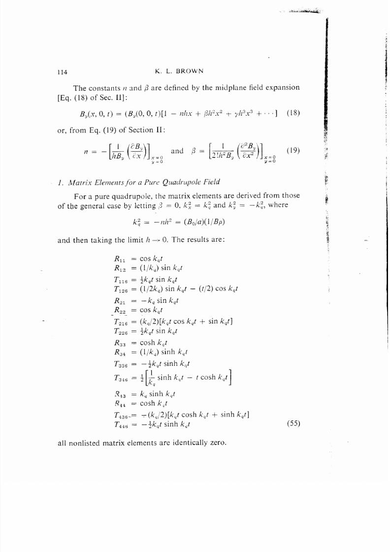
For a pure quadruple, the matrix elements are derived from those
~ = O. k: = k; and k; = —k:, wheref the general case by letting:~
k: = – ]1112= (BO/a)(l/Bp)
and then taking the limit /Z~ O. The results are:
R,, = COS k~t
R 12 = (l/k,) sin k,t
T 116 = ~k~t sin k~t
~,, = (1/2k,) sin kqt – (t/2) cos kqt
R 21 = –k, sin kqt
R 22 = COS k~t
‘T,lj = (kq/2)[kq? cos kqt + sin kqt]
T 226 = +kqt s in k qt
R = cosh kqt
R~~ = (l/kd) sinh k,t
T 336 = —~k~t sinh k,[t
T 346 = :[
~ sinh k,t – t cosh k~t——
q 1
.? 43 = k,, sinh k,t
R44 = cosh kit
T13G_= ~(kq/2)[kqt cosh k(,t+ sinh kqt]
T 446 = —~kqt sinh kqt (55)
all nonlisted matrix elements are identically zero.

5/12/2018 Accel Notes - slidepdf.com
http://slidepdf.com/reader/full/accel-notes 47/66
SYSTEM AN-D SI)EC”lROMETER DESIGN -115
2. Matri.~ E le ~?~e \ ~ts f or a P~rz Se.~tlipole Field
For a pure sextupole, the matrix elements are derived from thoseof the general case by letting
p)l’ = k; = (B,,’a2)(l /Bp)
and then taking the limit 1/~ O. The results are:
R,l =1
Rt12 =
T —+,~:t~111 =
T _+~;t3112 =
T ~Q~= –-l~fk:t’
T1Z3 = ~k;tz
T +~:t3134 ‘.
T -~-kzt ~144= 12 s
R 2 1 = 0R 22 = 1
T211 = –k:t
T 212 =–k:t2
T222 = –~k;t3
T 23 3 = k:t
T 234= ~:[2
T1~2 3
244 = ~ ~t
R = 1—R;; -=t
T 31 3= k :t 2
Tlh.2 3
31 4 =Tst
Tlk2 3
323 =~~t
T ~k2t4324=6s
R 43 = 0R14 =
T 41 3 = 2k;t
T 4 1 4 = k ; t 2
T 423 = kft2
- T4~4 = ~k?t3 (56)
All nonlisted matrix elements are identically zero.

5/12/2018 Accel Notes - slidepdf.com
http://slidepdf.com/reader/full/accel-notes 48/66
116 K. L. BRO\VN‘,.,’,-%,e
3. First- aII(l S eLo}I~/ -Or~/ cr ,J f~~rri.r El~~f)leflts jor a Cl{rre(i, Illclitled i’
.Ilog~~e[ic Fie[(f Bol{il(/ar~l.,,,~?!*-%
Nlfitrix elements for the fringing iields of bending magnets have ~
been derived using an impul~e ~ipproximati{~ll.’y~) These computations, ‘combined ~vith a correction term(g) to the R43 elements (to correct
for the finite extent of actual fringing fields), have produced results ‘
~vhich are in jubstarttial agreement with precise ray-tracing calculations
and ~~i[h experimental rne:lsurements made on actual magnets.
We introduce four ne~v \ariables (ii]ustrated in Fig. 11); the angle
of inclination ~1 of the entrance Pace of a bending magnet, the radius-of
curvature RI of the entrance fuce, the angle of inclination ~2 of the exit
face, and the radius of cur~ature RJ of the exit face. The jign con~ention
of~l and ,3: is considered positive for positi~e focusing in the transverse
(j) direction. The sign con~ention for R, and R, is positive if the fieldboundary is convex out\\ard: (a positi~e R represents a negative sextu-
pole component of strength. k~L = –(// ‘2R) jecJ ~). The sign conven-
tions adopted here are in agreement with Penner,(4) and Brown,
Belbeoch, and Bounin.(7)
\
\>\/,
+Z1
/
‘,
‘ “\,‘y,
R2/A
/
4
,’
/
po= I/ h
,//
FIG. 11. Field boundaries for bending magnets.
PI, ~~, Rl, and R, used in the matrix elements for field boundaries of bending
Definition of the quantities
magnets. The quantities have a positive sign convention as illustrated in the figure.

5/12/2018 Accel Notes - slidepdf.com
http://slidepdf.com/reader/full/accel-notes 49/66
SYSTEM AND SPECTROMETER DESIGN 117
The results of these calculations yield the following matrix elementsfor the fringing fields of the entrance face of a bending magnet:
R –13 —
RO4 =
T 313 = /7 tan2 PI
All nonlisted matrix elements are equal to zero. The quantity 41 is the
correction to the transverse focal length when the finite extent of the
fringing field is included.(g)
~~1= Kjlg sec ~1(1 + sin2 ~1) + higher order terms in (hg)
where g = the distance between the poles of the magnet at the central
orbit (i. e., the magnet gap) and
BU(D)is the magnitude of the fringing field on the magnetic nlid-
plane at a position =. Gis the perpendicular (iistance measured from the
entrance Pdce of the magnet to the point in question. B. is the asynlpt(>tic
value of B,(z) well inside the magnet entrance. Tvpica] ~’alues of h- ft>r
actual magnets may range from 0.3 to 1.0 depending upon the detailed
shape of the magnet profile and the location of the energizing coils.

5/12/2018 Accel Notes - slidepdf.com
http://slidepdf.com/reader/full/accel-notes 50/66
118 K. L. BROWN
The matrix elements for the fringing fields of the exit face of a
bending magnet are:
R ,l =
R 1 2 =
T 111 =
T 1 3 3 =
R21 =
R 22 =
T 211 =
T 212 =
T 2 1 6 =
T 233 =
T 234 =
R 33 =
R 34 =
T 313 =
R 43 =
R 44 =
T 4 1 3 =
1
0
(h / 2 ) tan2 ~2
– (h/2) sec2 ~2
–l/fX =htan P2
1
(h/2 R,)sec3P2 –h2(n +~tan2~2)tan~2
– h tan2 ~2–h tan ~2
h2(n – ~ tan2 ~2) tan ~2 – (h/2R2 sec3 ~2
h tan2 ~2
1
0
–JI tanz ~z
–l/fv = –h tan (F2 – +2)
1
–(J7/R2)sec3~2 +h2(2n+ sec2~2)tan P2
1 4 1 4 = JI t a n 2 ~ 2
T 4 2 3 = h sec2 ~z
T43, = Jz tan ~2 - hYzsec2(@z - @z)—
All nonlisted matrix elements are zero.
(58)
42 = Khg sec P,(1
and K is evaluated for
+ sin2 ~z) + higher order terms in (hg)
the exit fringing field.
4. Matrix Eiementsfor a Dr\~t Distance
For a drift distance of length L, the matrix eleme~ts are simply as
follows:
:.,?.
R,, = R,, “= R~, = R44 = RJ5 = R,’j = 1
R12 = R34 = L
All remaining first- and second-order matrix elements are zero.

5/12/2018 Accel Notes - slidepdf.com
http://slidepdf.com/reader/full/accel-notes 51/66
IV.
SYSTEM AND SPECTROMETER DESIGN 119
Some Useful First-Order Optical Results Derived
from the General Theory of section II (1011)
We have shown in Section II, Eq. (47), that beam transport optics
may be reduced to a process of matrix multiplication. To first order,
this is represented by the matrix equation
X1(l) = $ R, , . Y , ( o ) (j9)J=l
where
We” have also proved that the determinant IR I = 1 results from the
basic equation of motion and is a manifestation of Lioutille’s theorem
of conservation of phase space volume.
The six simultaneous linear equations represented by Eq. (j9) may
be expanded in matrix form as follows:
1x(t)
e(t?
y(t)
~(t)
l(t)
8(t)
——
where the transform
pOsitiOn T = t .
R,l Rlz O 0 0 R,,
R ~1 R,z O 0 0 R,,
o 0 R,, R3, O 0
0 0R,, R,, O 0
R ,1 R,, O 0 1 R,,
000001,
x~
e.
Yo
To
/ 0
80
(60)
ion is from an initial position 7 = L to a final
The zero elements R13 = RIA = Rz~ = RZ4 = R~l = RaQ = R.ll
= R,lz = R3G = RqG = O in the R matrix are a direct consequence of
midplane symmetry. If midplane symmetry is destroyed, these elements
will in general become nonzero. The zero elements in column five occur
because the variables x, e, ~. p, and 8 are independent of the pathlength difference 1.The zeros in row six result from the fact that we have
restricted the problem to static magnetic fields, i.e., the scalar momentum
is a constant of the motion.
We have already attached a physical significance to the nonzero
matrix elements in the first %ur~ows in terms of their identification with
characteristic first-order trajectories. We now wish to relate the elements
appearing in column six with those in row five and calculate both sets

5/12/2018 Accel Notes - slidepdf.com
http://slidepdf.com/reader/full/accel-notes 52/66
120 K. L. BROWN
in terms of simple integrals of the characteristic first-order elements
cX(t) = Rll and s.(t) = Rlz. In order to do this, we make use of theGreen’s integral, Eq. (43) of Section II, and of the expression for the
differential path length in curvilinear coordinates
dT = [(d.Y)2 + (dy)2 + (1 + hx)2(dt)2]’2 (61)
used in the derivation of the equation of motion.
1. First-Order Dispersion
The spatial dispersion dx(t) of a system at position t is derived
using the Green’s function integral, Eq. (43), and the driving term~ = h ( T )for the dispersion (see Table 1). The result is
-t
J j
t
dX(t) = Al, = S T ( f ) Cx(T)h(T) dr – cX(t) S..(7)/?(7) d7 (62)o 0
where T is the variable of integration. Note that h(7) dT = da is the
differential angle of bend of the central trajectory at any point in the
system. Thus first-order dispersion is generated only in regions where
the central trajectory is deflected (i.e., in dipole elements.) The angular
dispersion is obtained by direct differentiation of dY(t) with respect to t;
j
t
d:(t ) = R2, = ~i(f)
j
cx(T)h(T) d7 – cj(t) f sX(~)/?(7) d~ (63)o 0
where
—c:(t) = R21 and s~(r) = R22-
2. First-Order Path Length
The first-order path length difference is obtained by expanding
Eq. (61) and retaining only the first-order term, i.e.,
/
t
/–lo=(T– t)= X ( T )h (T ) dT + higher order termso
from which
J
t
j
t
/ =x.
j
t
cX(T)h(T) dr + 60 sX(7)h(7) dT + /0 + 8 dy(T)/l(T) dT
o 0 0
= RSIXO + R5260 + 10 + R56~ (64)

5/12/2018 Accel Notes - slidepdf.com
http://slidepdf.com/reader/full/accel-notes 53/66
SYSTEM AND SPECTROMETER DESIGN 121
Inspection of Eqs. (62)–(64)yie1ds the following useful theorems:
A. Achrornaticity
A system is defined as being achromatic if dy(t) = di(t) = O.
Therefore it follows from Eqs. (62) and (63) that the necessary and
sufficient conditions for achromaticity are that
Jt
Jt
s-y(T)h(T)dT = cx(T)h(T)dT = o0 0
(65)
Bycomparing Eq. (64) with Eq. (65), wenotethat ifasystemisachro-
matic, all particles of the same momentum will have equal (first-order)
path lengths through the system.
B. Isochronicity
It is somewhat unfortunate that this word has been used in the
literature: since it is applicable -only to highly relativistic particles.
Nevertheless, from Eq. (64) the necessary and sufficient conditions that
the first-order path length of all particles (independent of their initial
momentum) will be the same through a system are that
j
t
j
t
j
t
cX(7)h(7) d7 = sy(r)h(7) dT = dX(T)h(T) d~ = O (66)o 0 0
3. First-Order Imaging
First-order point-to-point imaging in the x plane occurs when x(t)
is independent of the initial angle 8.. This can only be so when—
s.(t) = R12 = o (67)
Similarly, first-order point-to-point imaging occurs in the y plane when
Su(t) = R~4 = o
First-order parallel-to-point imaging occurs
is independent of the initial particle position
Cx(t) = Rll = o
(68)
in the x plane when x(t)
Xo. This will occur only if
(69)
and correspondingly in the y plane, parallel-to-point imaging occurs
when
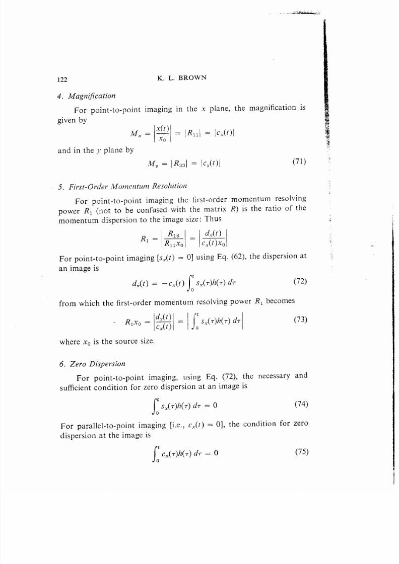
5/12/2018 Accel Notes - slidepdf.com
http://slidepdf.com/reader/full/accel-notes 54/66
122 K. L. BROWN
4. Magnl~cation
For point-to-point imaging in the x plane, the magnification is
given by
.Y(tM. = — = 1~1,1= lc ,x(~)lXo
and in the ]’ plane by
M, = IR331 = Ic,(f)l (71)
5. First-Order lMotnentu~?z Resolution
For point-to-point imaging the first-order momentum resolving
power RI (not to be confused with the matrix R) is the ratio of the
momentum dispersion to the image size: Thus
R dy(t )R, = — =
R1~;o Cx(t)xo
For point-to-point imaging [sX(t) = O] using Eq. (62), the dispersion at
an image is
)x(t) = – c.%(t) “SX(r)~(7) d7 (72)o
from which the first-order momentum resolving power RI becomes
dY(t )
J
t
- ~lxo -= — = Sx(T)h(T) dTCx(t ) o
(73)
where X. is the source size.
6. Zero Dispersion
For point-to-point imaging, using Eq. (72), the necessary andsufficient condition for zero dispersion at an image is
JtSx(T)h(T) dT = O
0(74)
For parallel-to-point imaging [i.e., cX(t) = O], the condition for zero
dispersion at the image is
.“
!tCx(T)h(T)d7 = O (75)
o
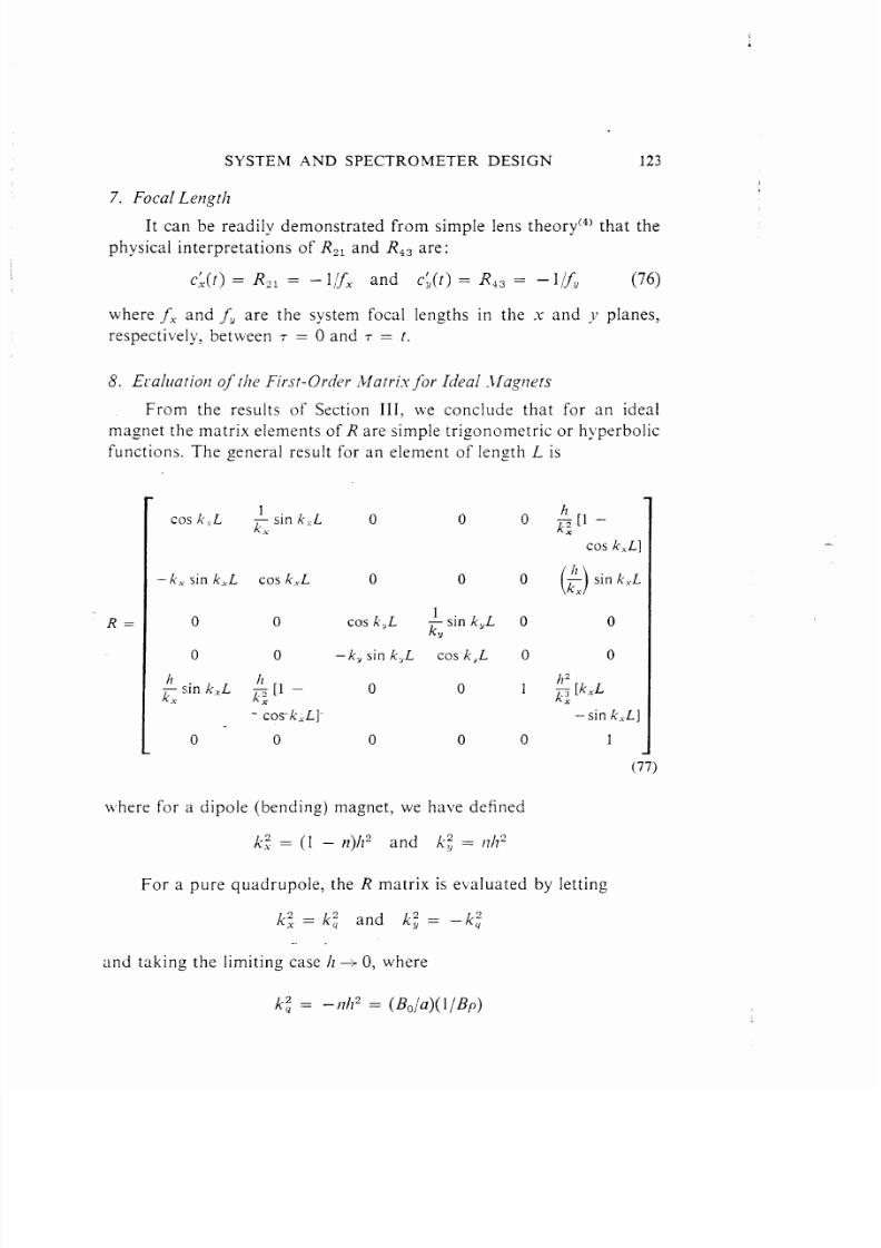
5/12/2018 Accel Notes - slidepdf.com
http://slidepdf.com/reader/full/accel-notes 55/66
SYSTEM AND SPECTROMETER DESIGN 123
7. Focal Let~gtll
It can be readily demonstrated from simple lens theory(4) that the
physical interpretations of Rzl and RA3are:
c~(f) = RQ1 = – I/fx and c~(r) = R+3 = – l/~Y (76)
where ~X and fv are the system focal lengths in the .~ and y planes,
respectively? between ~ = Oand 7 = t.
8. E1’alliatiorl of tile First-Order ~Matri.~for I~ieai .ifagr~ets
From the results of Section III, we conclude that for an ideal
magnet the matrix elements of R are simple trigonometric or hyperbolic
functions. The general result for an element of length L is
R=
1 sin~Lcos k,L
E “’o 0
–kx sin kxL cos k.yL o 0
00
lsink Lcos kvL
~y
o 0 –k, sin k,L COS kgL
I
h
Esin k.xL ;[l - 0 0
[
- corkxL]
o- 0 0 0
0
0
0
0
COSkxL]
o
0
; [kxLx
– sin k.xL]
1
(77)
where for a dipole (bending) magnet, we have defined
For a pure quadruple, the R matrix is evaluated by letting
k: = k; and k; = –k;
and taking the limiting case /Z-0, where
k: = – /?lz2= (BO/a)(l/Bp)

5/12/2018 Accel Notes - slidepdf.com
http://slidepdf.com/reader/full/accel-notes 56/66
... +
124 K. L. BROWN
Taking these limits, the R matrix for a quadruple is:
R=
1COSk~L
~sin kqL o 0 0 0
– k, sin k,L COSk~L o 0 0 0
0 0 cosh kQL # sinh k~L O 0q
o 0 kq sinh kqL cosh kqL O 0
0 0 0 0 1 0
0 0 0 0 0 1L
(78)
Note, that the trigonometric and hyperbolic functions wil! interchange
if the sign of BOis reversed.
9. The R Matri.~ Transfornled to the Principal Planes
The positions Z of the principal planes of a magnetic element
(measured from its ends) may be derived from the following matrix
equation:
RPP =
—
100 OoxRlo1 Oox
001 000
0 0 R,, 100
xx00
1 –Z,x o 0
0100
0 0 1 –Zz,
0001
0000
0000
0 0
00
0 0
0 0
10
01
Solving this equation, tie have
21X = (Rzz– 1)/R21
R
Xxxx
o 001.
I–zl,yoooo
01000000 1 –z,, o 0
000100
000010
000001
22X = (Rll – 1)/R21
Z2V= (R3q– 1)/R43
(79)
(80)

5/12/2018 Accel Notes - slidepdf.com
http://slidepdf.com/reader/full/accel-notes 57/66
SYSTEM AND SPECTROMETER DESIGN 125
For the ideal magnet, the general result for the transformation
matrix RPP between the principal planes is
R PP =
1 0 0 0 0 0
–k,r sin kxL 1 0 0 0 (/~k.,) sin k.,L
o 0 1 0 0 0
0 0 – k, sin kyL 1 0 0 (81)
(82)
Correspondillgly, for the ideal quadruple, R,,p is deri~’ed by
letting
k?. = k: and k; = –k:
and taking the limit 1?+ O for each of the matrix elenlents. The result
is:
I
1 0 0 0 0 0
–k , sin kqL 1 0 0 0 0
I@-
PP= o
I o
1 0
0 1 0 0 0
0 kq sinh k,L 1 0 0
0
0
00
0
0
where now
Z. = (l/k,) tan (k,L/2)
Z, = (l/k,) tanh (kqL12)
1
0
0
1-
(83) -
( 84)
V. Some General Second-OrderTheorems Derived fromthe General Theoryof Section II
-.We have established in Section 11 that any second-order aberra-
tion coefficient q may be evaluated via the Green’s function integral,
Eq. (43), i.e.,
q =J
s(t) ‘J(T)C(T) dT –I
c(t) ‘f(T)s(T) dTo 0
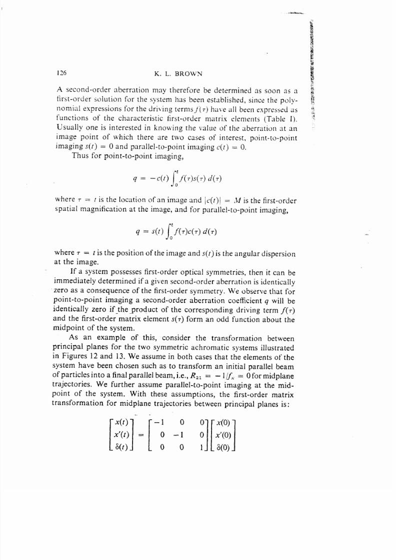
5/12/2018 Accel Notes - slidepdf.com
http://slidepdf.com/reader/full/accel-notes 58/66
-----
K. L. BROWN
A second-order aberration may therefore be determined as soon as a ~..4*
first-order solution for the system has been established, since the poly - ~
nomiai expressions for the driving termsj(~) ha~e ~ill been expressed tis j,
functions of the characteristic first-order matrix elements (Table 1)..!
Usually one is interested in knoyving the value of the aberration at an
image point of which there are two cases of interest, point-to-point
imaging s(l) = Oand parallel-to-point imaging c(r) = O.
Thus for point-to-point imaging,
where r = { is the locution of an image and ~c~(f)l= ,Mis the first-order
spatial magnification at the image, and for parallel-to-point imaging,
where ~ = r is the position of the image and s(f) is the angular dispersion
at the image.
If a system possesses first-order optical symmetries, then it can be
immediately determined if a given second-order aberration is identically
zero as a consequence of the first-order symmetry. We observe that for
point-to-point imaging a second-order aberration coefficient q will be
identically zero if_the_product of the corresponding driving term J(7)
and the first-order matrix element s(7) form an odd function about the
midpoint of the system.
As an example of this, consider the transformation between
principal planes for the two symmetric achromatic systems illustrated
in Figures 12 and 13. We assume in both cases that the elements of the
system have been chosen such as to transform an initial parallel beam
of particles into a final parallel beam, i.e., Rzl = —l/~X= Ofor midplane
trajectories. We further assume parallel-to-point imaging at the mid-
point of the system. With these assumptions, the first-order matrix
transformation for midplane trajectories between principal planes is:
[
x(t) .
x’(t)
~(t) . [
–1 o 0= o –1 o
001
x(o)
x’(o)
8(0)1

5/12/2018 Accel Notes - slidepdf.com
http://slidepdf.com/reader/full/accel-notes 59/66
SYSTEM AND SPECTROMETER DESIGN127
B’
FIG. 12. Three bending magnet achromatic system. A and B are locations ofprincipal planes.
Thus c.y(~) = – 1> ~.Y(~)= ‘~ c~(f) = ‘~ ‘~(t) = – 1’ and ‘f course
d.(r) = d~.(r) = O. About the midpoint of the system, the followlng
symmetries exist for the characteristic first-order matrix elements and
for the curvature ~~(~)= l/pO of the central trajectory; we classify them
as being either odd or even functions about the midpoint of the system.
The results are:
dx(T) = even /2(r) = evencY(7) = odd s,,(T) = even
s~(7) = odd d~(7) = odd j?’(~) = oddc;.(7) = even
/—
c ~ AI/
trajectory PO
-. Cx
FIG. 13. Achromatic system with quadruple at center to achieve achromatic
imaging. The principal planes are located at centers of the bending magnets.

5/12/2018 Accel Notes - slidepdf.com
http://slidepdf.com/reader/full/accel-notes 60/66
128 K. L. BROWN
As a consequence of these symmetries, the following second-order
coefficients are uniquely zero for the transformation between principal
planes.
This result is valid, independent of the details of the fringing fields of
the magnets, provided symmetry exists about the midpoint.
I. Optical Symmetries in n = &Magnetic SJ’stems
In magnetic optical systems composed of n = j magnets havingnormal entry and exit of the central trajectory (i.e., nonrotated entrance
and exit faces), several general mathematical relationships result from
the n“= ~ symmetry. Since k: = (1 – n)hz and k: = nh”, for n = 4
it follows that CX(7)= CU(T) and SX(T) = SU(T) at any position r along
the system; thus as is well known, an n = ~ system possesses first-order
double focusing properties.
In addition to the above first-order results, at any point t in an
n = ~ system, the sums of the following second-order aberration
coefficients are constants independent of the distribution or magnitude
(~h3) of the sextupole components throughout the system:
(X IX:2) + (x IYi2) = a constant independent of ~h3
2 (x I x;) + (Y I XOYO) = a constant independent of ~h3
(X IXOXi~+ (Y I~oYh) = a Gonstant independent of #h3
(X IXO$)+ (Y IY08)= a constant independent of ~h3
2(x IX:2) + (Y I x~y~) = a constant independent of ~h3
(X Ix:8) + (Y IY&8)= a constant independent of ~h3
(X I x3) + (X [ y:) = a constant independent of ~h3
(X\ XOX~)+ (XI YOYj)= a constant independent of ~h3 (85)
Similarly,
(x’ \ x~2) + <x’ l-y&2)= a constant independent of #h3
2(x’ I x:) + (y’ I Xoyo) = a constant independent of ~h3
.,”
(X’ I xox~) + (y’ IXoy:) = a constant independent of ~h 3

5/12/2018 Accel Notes - slidepdf.com
http://slidepdf.com/reader/full/accel-notes 61/66
SYSTEM AND SPECTROMETER DESIGN 129
(x’ I x,8) + (~’ I ~o~) = a constant independent of ~A3
2(x’ ] X:2) + (~’ I x~~~) = a constant independent of ~k3
(x’ j X~8) + (~’ ] ~~~) = a constant independent of ~k3
(x’ \ x8) + (x’ \ Y;) = a constant independent of ~}t3
(x’ ] XOxj) + (x’ ] yoy~) = a constant independent of ~A3 (86)
Of the above relations, the first is perhaps the most interesting in that
it shows the impossibility of simultaneously eliminating both the(x IX:2)and (x Iy~2)aberrations in an n = ~ system; i.e., either (x IX:2)
or (x IyJ2) may be eliminated by the appropriate choice of sextupole
elements, but not both.
VI. An Approximate Evaluation of the Second-Order
Aberrations for High-Energy Physics
Quite often it is desirable to estimate the magnitude of various
second-order aberrations in a proposed system to obtain insight into
what constitutes an optimum solution to a given problem. A consider-
able simplification occurs in the formalism in the high-energy limit
where POis very much greater than the transverse amplitudes of the -
first-order trajectories and where the dipole, quadruple, and sextupole
functions are physically separated into individual elements. It is also
assumed that fringing-field effects are small compared to the contribu-
tions of the various multipole elements.
Under these circumstances, the second-order chromatic aberrations
are generated predominately in the quadruple elements; the geometric
aberrations are generated in the dipole elements (bending magnets); and,
depending upon their location in the system, the sextupole elements
couple with either the chromatic or geometric aberrations or both.
We have tabulated in Tables VII–IX the approximate formulas for
the high-energy limit for three cases of interest: point-to-point imaging
in the x (bend) plane, Table VII; point-to-point imaging in the y
(non bend) plane, Table VIII; and parallel-to-point imaging in the y
plane, Table IX.

5/12/2018 Accel Notes - slidepdf.com
http://slidepdf.com/reader/full/accel-notes 62/66
130 K. L. BROWN
TABLEVII
Applying the Greens’ Function Solution, Eq. (22), in the High-Energy Limit
as Defined Above for Point-to-Point Imaging in the x (bend) Plane, theSecond-Order Matrix Elements Reduce to the Values Shown
TABLE VIII
For Point-to-Point Imaging in they (nonbend) Plane, Eq. (23), the
HQh-Energy Limit Yields the Values Given

5/12/2018 Accel Notes - slidepdf.com
http://slidepdf.com/reader/full/accel-notes 63/66
SYSTEM AND SPECTROMETER DESIGN
TABLEIX
For Parallel-( Line) -to-Point Imaging in the y (Nonbend) Plane,
the High-Energy Limit Yields the Values Shown
131
Eq. (24),
For the purpose of clearly illustrating the physical principles in-
volved, we assume that the amplitudes of the characteristic first-ordermatrix elements CX,SX,dx, Cy,and Su are constant within any given
quadruple or sextupole element, and we define the strengths of the
quadruple and sextupole elements as follows:
/
L
k: dr = k:L~ z ~o f,
,, where Lq is the effective length of the quadruple, and where l/ f~ = k,
sin kQL is the reciprocal of the focal length of the gth quadruple; andI
for the jth sextupole of length L,, we define its strength as;,
I
1
L~,
k: dr = k~L, = S,o
!,The results are given in the tables in terms of integrals over the bending
magnets and summations over the quadruple and sextupole elements.
Note that under these circumstances the quadruple and sextupole
/ contributions to the aberration coefficients are proportional to the
amplitudes of the characteristic first-order trajectories within these
elements, whereas the dipole contributions are proportional to the
derivatives of the first-order trajectories within the dipole elements.!
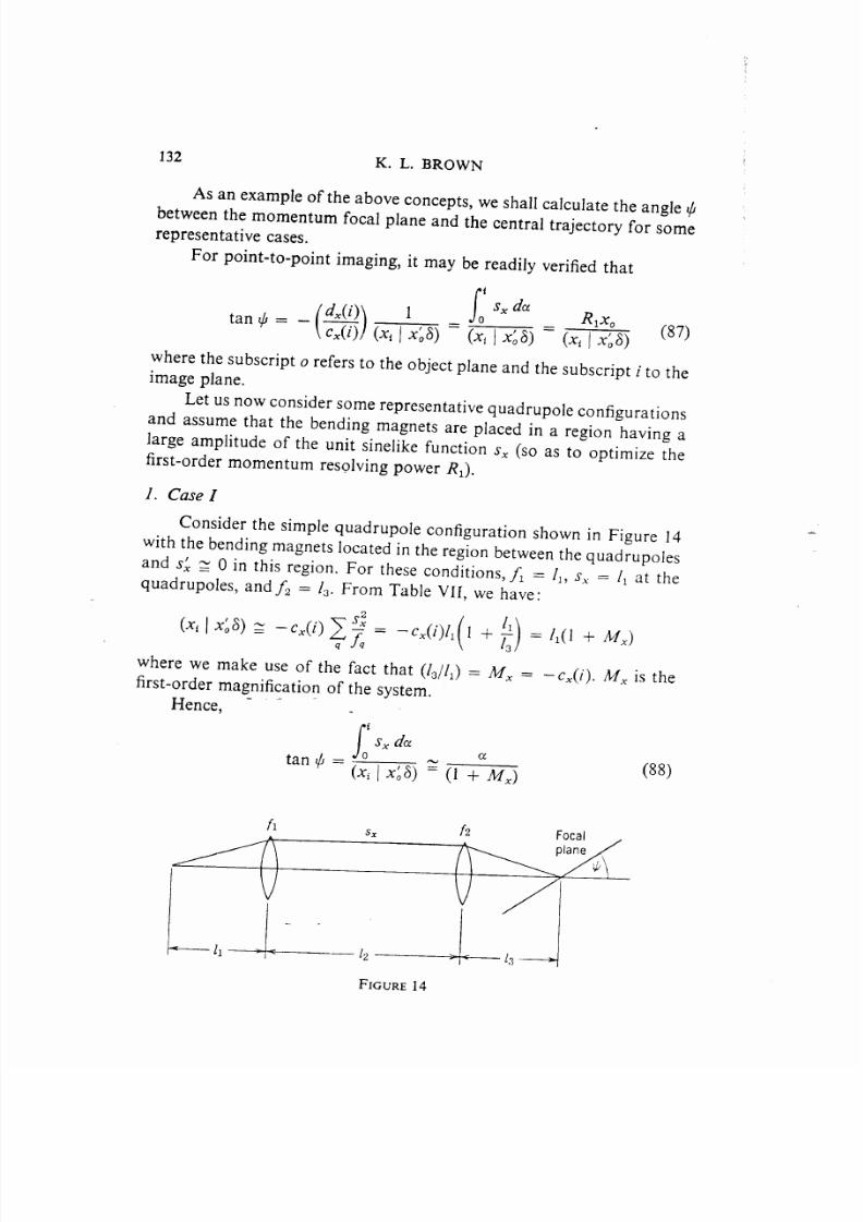
5/12/2018 Accel Notes - slidepdf.com
http://slidepdf.com/reader/full/accel-notes 64/66
132K. L. BROWN
As an example of the above concepts, we shall calculate the angle #
between the momentum focal plane and the central trajectory for some
representative cases.
For point-to-point imaging, it may be readily verified that
!f
dx(i) 1
()Sx da
tan+=– — A,xoCx(i) m ) = *) = (= (87)
where the subscript o refers to the object plane and the subscript i to the
image plane.
Let us now consider some representative quadruple configurations
and assume that the bending magnets are placed in a region having a
large amplitude of the unit sinelike function SX(so as to optimize the
first-order momentum resolving power R,).
Consider the simple quadruple configuration shown in Figure 14with the bending magnets located in the region between the quadruples
and s: ~ Oin this region. For these conditions, ~1 = 11,SX= 11at the
quadruples, and ~z = /3. From Table VII, we have:
where we make use of the fact that (/3/[1) = MX = – cX(i). M. is the
first-order magnification of the system.
Hence, - - _
/
tS. da
tan~=.o
(xl I Xj8) = a (88)
fl Sx fz Focal
P i-.
I
F IGURE 14
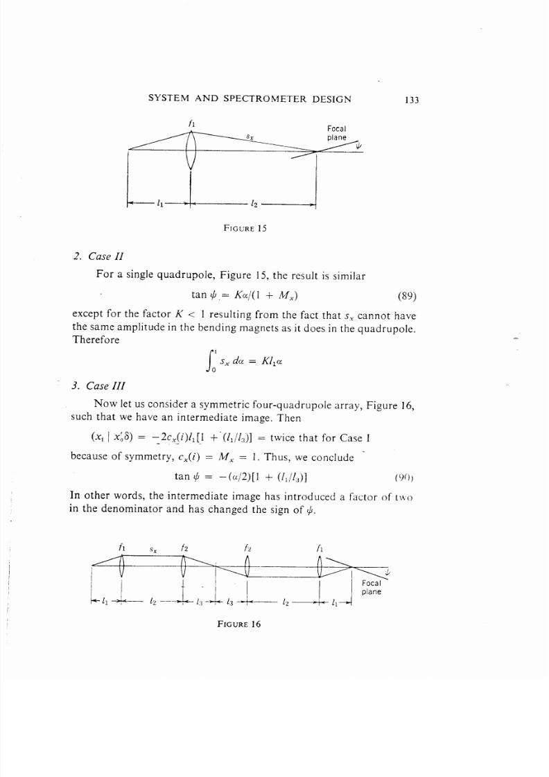
5/12/2018 Accel Notes - slidepdf.com
http://slidepdf.com/reader/full/accel-notes 65/66
SYSTEM AND SPECTROMETER DESIGN 133
flFocalplane
/$
I
FIGURE 15
2. Case IIFor a single quadruple, Figure 15, the result is similar
tan #.= Ka/(1 + MX) (89)
except for the factor K < 1 resulting from the fact that s, cannot have
the same amplittie in the bending magnets as it does in the quadruple.
Therefore
3. Case III
Now let us consider a
/
i
SX da = K!lao
symmetric four-q uadrupole array, Figure 16,
such that we have an intermediate image. Then
(x, I x:$) = –2cX(i)ll[l +“(11//,)] = twice that for Case I—
because of symmetry, cX(i) = MX = 1. Thus, we conclude -
tan ~ = –(a/2)[1 + (~~/~s)l (90)
In other words, the intermediate image has introduced a factor of t;vo
in the denominator and has changed the sign of ~.
FIGURE 16

5/12/2018 Accel Notes - slidepdf.com
http://slidepdf.com/reader/full/accel-notes 66/66
134
1.
2.
3.
4.
5.
6.
7.
8.
9.
10.
K. L. BROWN
References
J. F. Streib, “Design Considerations for Magnetic Spcctrometcrs, ” HEPL
Report NCJ. 104, High-Energy Physics Laboratory, Stanford University,
Stanford, California ( [960).
L. C. Teng, “Expanded Form of ,Magnctic Field with Median Plane, ” ANLlntcrnal Memorandum AN L-LCT-28 (Dcccmbcr 15, 1962).
K.L. Brom, D.C. Carey, Ch. Iselin, and F. Rothacker,
“TWSPORT A Computer Program for Designing Charged
Particle Beam Transport Systems,” SMC-91 (1973 Rev.),
NW-91, and CERN 80-04.
S. Penner, ‘. Calculations of Properties of lMagnetic Deflection Systems, ” in
Rell. Sci. /nsrr., 32, No. 2, 150-160 (1961).
K. G. Steffen, Hi~/1 Etlerg> Beam Opric.~ (Monographs and Texts in Physics
and Astronomy, Vol. 17, R. E. Marshak, Ed.), lntcrsciencc, Ncw York, 1965.
A. P. Ban ford, Tlle Trutlsport oj C/lurge~i Purtit /e Beat)l.s, Sp(~n. L[d.. London.
1966.
K. L. Brown, R. Belbeoch. and P. Bounin, ” First-and Second-Order MagneticOptics Matrix Equations for (hc hlidplane of Unif~)rm-l;ield \Vcdge ,Magncts.
in Ret. Sci. /)ls[r.. 35, 481 ( 1964) (SLAC-PUB-19),
R. H. HC]I1l, “First - and Second-Order Beam Optics of a Curvcci. Inclined
Magnetic Field Boundary in the lmpulsc Approxilll;]tl[)rl... SL,\C Rcp~>rt
No. 24. Stanford Linear .Accclerator Center, S(anford, Ctilift)rnia ( 1963).
A. C. Hindmarsh an d K. L. Brown, the express ion f[)r IJj and II,, w~s calcu-
lated in hnpublishcd work, at SLAC for inscr[ion into the TRANSPORT
Program:
K. L. Brown. “Some Useful Thcorenls Based on a General First-Order
Theory of Image Formation, “SLAC lntcrnal Report, TN-64-18, Stanford
Linear Accelerator Cen[er, Stanford, California.
..,,
--