Academic Press is an imprint of Elsevier Library... · 2018-11-05 · of distributed source...
340
Transcript of Academic Press is an imprint of Elsevier Library... · 2018-11-05 · of distributed source...

Academic Press is an imprint of Elsevier30 Corporate Drive, Suite 400, Burlington, MA 01803, USA525 B Street, Suite 1900, San Diego, California 92101-4495, USA84 Theobald’s Road, London WC1X 8RR, UK
This book is printed on acid-free paper. �©Copyright © 2009, Elsevier Inc. All rights reserved.
No part of this publication may be reproduced or transmitted in any form or by any means,electronic or mechanical, including photocopy, recording, or any information storage andretrieval system, without permission in writing from the publisher.
Permissions may be sought directly from Elsevier’s Science & Technology Rights Department inOxford, UK: phone: (+44) 1865 843830, fax: (+44) 1865 853333, E-mail: [email protected] may also complete your request on-line via the Elsevier homepage (http://elsevier.com), byselecting “Customer Support”and then “Obtaining Permissions.”
Library of Congress Cataloging-in-Publication DataDragotti, Pier Luigi.
Distributed source coding :theory, algorithms, and applications / Pier Luigi Dragotti,Michael Gastpar.
p. cm.Includes index.ISBN 978-0-12-374485-2 (hardcover :alk. paper)
1. Data compression (Telecommunication) 2. Multisensor data fusion. 3. Coding theory.4. Electronic data processing–Distributed processing. I. Gastpar, Michael. II. Title.
TK5102.92.D57 2009621.382�16–dc22
2008044569
British Library Cataloguing in Publication DataA catalogue record for this book is available from the British Library
ISBN 13: 978-0-12-374485-2
For information on all Academic Press publicationsvisit our Web site at www.elsevierdirect.com
Printed in the United States of America09 10 9 8 7 6 5 4 3 2 1
Typeset by: diacriTech, India.

List of Contributors
Chapter 1. Foundations of Distributed Source Coding
Krishnan EswaranDepartment of Electrical Engineering and Computer SciencesUniversity of California, BerkeleyBerkeley, CA 94720
Michael GastparDepartment of Electrical Engineering and Computer SciencesUniversity of California, BerkeleyBerkeley, CA 94720
Chapter 2. Distributed Transform Coding
Varit ChaisinthopDepartment of Electrical and Electronic EngineeringImperial College, LondonSW7 2AZ London, UK
Pier Luigi DragottiDepartment of Electrical and Electronic EngineeringImperial College, LondonSW7 2AZ London, UK
Chapter 3. Quantization for Distributed Source Coding
David Rebollo-MonederoDepartment of Telematics EngineeringUniversitat Politècnica de Catalunya08034 Barcelona, Spain
Bernd GirodDepartment of Electrical EngineeringStanford UniversityPalo Alto, CA 94305-9515
xiii

xiv List of Contributors
Chapter 4. Zero-error Distributed Source Coding
Ertem TuncelDepartment of Electrical EngineeringUniversity of California, RiversideRiverside, CA 92521
Jayanth NayakMayachitra, Inc.Santa Barbara, CA 93111
Prashant KoulgiDepartment of Electrical and Computer EngineeringUniversity of California, Santa BarbaraSanta Barbara, CA 93106
Kenneth RoseDepartment of Electrical and Computer EngineeringUniversity of California, Santa BarbaraSanta Barbara, CA 93106
Chapter 5. Distributed Coding of Sparse Signals
Vivek K GoyalDepartment of Electrical Engineering and Computer ScienceMassachusetts Institute of TechnologyCambridge, MA 02139
Alyson K. FletcherDepartment of Electrical Engineering and Computer SciencesUniversity of California, BerkeleyBerkeley, CA 94720
Sundeep RanganQualcomm Flarion TechnologiesBridgewater, NJ 08807-2856
Chapter 6. Toward Constructive Slepian–Wolf Coding Schemes
Christine GuillemotINRIA Rennes-Bretagne AtlantiqueCampus Universitaire de Beaulieu35042 Rennes Cédex, France

List of Contributors xv
Aline RoumyINRIA Rennes-Bretagne AtlantiqueCampus Universitaire de Beaulieu35042 Rennes Cédex, France
Chapter 7. Distributed Compression in Microphone Arrays
Olivier RoyAudiovisual Communications LaboratorySchool of Computer and Communication SciencesEcole Polytechnique Fédérale de LausanneCH-1015 Lausanne, Switzerland
Thibaut AjdlerAudiovisual Communications LaboratorySchool of Computer and Communication SciencesEcole Polytechnique Fédérale de LausanneCH-1015 Lausanne, Switzerland
Robert L. KonsbruckAudiovisual Communications LaboratorySchool of Computer and Communication SciencesEcole Polytechnique Fédérale de LausanneCH-1015 Lausanne, Switzerland
Martin VetterliAudiovisual Communications LaboratorySchool of Computer and Communication SciencesEcole Polytechnique Fédérale de LausanneCH-1015 Lausanne, SwitzerlandandDepartment of Electrical Engineering and Computer SciencesUniversity of California, BerkeleyBerkeley, CA 94720
Chapter 8. Distributed Video Coding: Basics, Codecs, andPerformance
Fernando PereiraInstituto Superior Técnico—Instituto de Telecomunicações1049-001 Lisbon, Portugal

xvi List of Contributors
Catarina BritesInstituto Superior Técnico—Instituto de Telecomunicações1049-001 Lisbon, Portugal
João AscensoInstituto Superior Técnico—Instituto de Telecomunicações1049-001 Lisbon, Portugal
Chapter 9. Model-based Multiview Video Compression UsingDistributed Source Coding Principles
Jayanth NayakMayachitra, Inc.Santa Barbara, CA 93111
Bi SongDepartment of Electrical EngineeringUniversity of California, RiversideRiverside, CA 92521
Ertem TuncelDepartment of Electrical EngineeringUniversity of California, RiversideRiverside, CA 92521
Amit K. Roy-ChowdhuryDepartment of Electrical EngineeringUniversity of California, RiversideRiverside, CA 92521
Chapter 10. Distributed Compression of Hyperspectral Imagery
Ngai-Man CheungSignal and Image Processing InstituteDepartment of Electrical EngineeringUniversity of Southern CaliforniaLos Angeles, CA 90089-2564
Antonio OrtegaSignal and Image Processing InstituteDepartment of Electrical EngineeringUniversity of Southern CaliforniaLos Angeles, CA 90089-2564

List of Contributors xvii
Chapter 11. Securing Biometric Data
Anthony VetroMitsubishi Electric Research LaboratoriesCambridge, MA 02139
Shantanu RaneMitsubishi Electric Research LaboratoriesCambridge, MA 02139
Jonathan S. YedidiaMitsubishi Electric Research LaboratoriesCambridge, MA 02139
Stark C. DraperDepartment of Electrical and Computer EngineeringUniversity of Wisconsin, MadisonMadison, WI 53706

Introduction
In conventional source coding,a single encoder exploits the redundancy of the sourcein order to perform compression. Applications such as wireless sensor and cameranetworks, however, involve multiple sources often separated in space that need tobe compressed independently. In such applications, it is not usually feasible to firsttransport all the data to a central location and compress (or further process) it there.The resulting source coding problem is often referred to as distributed source coding(DSC). Its foundations were laid in the 1970s, but it is only in the current decadethat practical techniques have been developed,along with advances in the theoreticalunderpinnings.The practical advances were,in part,due to the rediscovery of the closeconnection between distributed source codes and (standard) error-correction codesfor noisy channels. The latter area underwent a dramatic shift in the 1990s, followingthe discovery of turbo and low-density parity-check (LDPC) codes. Both constructionshave been used to obtain good distributed source codes.
In a related effort, ideas from distributed coding have also had considerable impacton video compression, which is basically a centralized compression problem. Inthis scenario, one can consider a compression technique under which each videoframe must be compressed separately, thus mimicking a distributed coding problem.The resulting algorithms are among the best-performing and have many additionalfeatures,including,for example,a shift of complexity from the encoder to the decoder.
This book summarizes the main contributions of the current decade.The chaptersare subdivided into two parts. The first part is devoted to the theoretical foundations,and the second part to algorithms and applications.
Chapter 1, by Eswaran and Gastpar, summarizes the state of the art of the theoryof distributed source coding, starting with classical results. It emphasizes an impor-tant distinction between direct source coding and indirect (or noisy) source coding:In the distributed setting, these two are fundamentally different. This difference isbest appreciated by considering the scaling laws in the number of encoders: In theindirect case, those scaling laws are dramatically different. Historically, compressionis tightly linked to transforms and thus to transform coding. It is therefore naturalto investigate extensions of the traditional centralized transform coding paradigm tothe distributed case. This is done by Chaisinthop and Dragotti in Chapter 2, whichpresents an overview of existing distributed transform coders. Rebollo-Monedero andGirod, in Chapter 3, address the important question of quantization in a distributedsetting. A new set of tools is necessary to optimize quantizers, and the chapter givesa partial account of the results available to date. In the standard perspective, efficientdistributed source coding always involves an error probability,even though it vanishesas the coding block length is increased. In Chapter 4,Tuncel, Nayak, Koulgi, and Rosetake a more restrictive view: The error probability must be exactly zero.This is shown
Distributed Source Coding: Theory, Algorithms, and ApplicationsCopyright © 2008 by Academic Press, Inc. All rights of reproduction in any form reserved. xix

xx Introduction
to lead to a strict rate penalty for many instances. Chapter 5, by Goyal, Fletcher, andRangan, connects ideas from distributed source coding with the sparse signal modelsthat have recently received considerable attention under the heading of compressed(or compressive) sensing.
The second part of the book focuses on algorithms and applications, where thedevelopments of the past decades have been even more pronounced than in the the-oretical foundations.The first chapter,by Guillemot and Roumy,presents an overviewof practical DSC techniques based on turbo and LDPC codes,along with ample exper-imental illustration. Chapter 7, by Roy, Ajdler, Konsbruck, and Vetterli, specializesand applies DSC techniques to a system of multiple microphones, using an explicitspatial model to derive sampling conditions and source correlation structures. Chap-ter 8, by Pereira, Brites, and Ascenso, overviews the application of ideas from DSCto video coding: A single video stream is encoded, frame by frame, and the encodertreats past and future frames as side information when encoding the current frame.Thechapter starts with an overview of the original distributed video coders from Berkeley(PRISM) and Stanford,and provides a detailed description of an enhanced video coderdeveloped by the authors (and referred to as DISCOVER). The case of the multiplemultiview video stream is considered by Nayak, Song, Tuncel, and Roy-Chowdhuryin Chapter 9,where they show how DSC techniques can be applied to the problem ofmultiview video compression. Chapter 10, by Cheung and Ortega, applies DSC tech-niques to the problem of distributed compression of hyperspectral imagery. Finally,Chapter 11, by Vetro, Draper, Rane, and Yedidia, is an innovative application of DSCtechniques to securing biometric data.The problem is that if a fingerprint, iris scan,orgenetic code is used as a user password, then the password cannot be changed sinceusers are stuck with their fingers (or irises,or genes).Therefore,biometric informationshould not be stored in the clear anywhere. This chapter discusses one approach tothis problematic issue, using ideas from DSC.
One of the main objectives of this book is to provide a comprehensive reference forengineers, researchers, and students interested in distributed source coding. Resultson this topic have so far appeared in different journals and conferences. We hopethat the book will finally provide an integrated view of this active and ever evolvingresearch area.
Edited books would not exist without the enthusiasm and hard work of thecontributors. It has been a great pleasure for us to interact with some of the verybest researchers in this area who have enthusiastically embarked in this projectand have contributed these wonderful chapters. We have learned a lot from them.We would also like to thank the reviewers of the chapters for their time and fortheir constructive comments. Finally we would like to thank the staff at AcademicPress—in particularTim Pitts, Senior Commissioning Editor, and Melanie Benson—fortheir continuous help.
Pier Luigi Dragotti, London, UK
Michael Gastpar, Berkeley, California, USA

CHAPTER
1Foundations of DistributedSource Coding
Krishnan Eswaran and Michael GastparDepartment of Electrical Engineering and Computer Sciences,
University of California, Berkeley, CA
C H A P T E R C O N T E N T SIntroduction . . . . . . . . . . . . . . . . . . . . . . . . . . . . . . . . . . . . . . . . . . . . . . . . . . . . . . . . . . . . . . . . . . . . . . . . . . . . . . 3Centralized Source Coding . . . . . . . . . . . . . . . . . . . . . . . . . . . . . . . . . . . . . . . . . . . . . . . . . . . . . . . . . . . . . . . 4
Lossless Source Coding . . . . . . . . . . . . . . . . . . . . . . . . . . . . . . . . . . . . . . . . . . . . . . . . . . . . . . . . . . . . 4Lossy Source Coding . . . . . . . . . . . . . . . . . . . . . . . . . . . . . . . . . . . . . . . . . . . . . . . . . . . . . . . . . . . . . . . 5Lossy Source Coding for Sources with Memory . . . . . . . . . . . . . . . . . . . . . . . . . . . . . . . . . . . . 8Some Notes on Practical Considerations . . . . . . . . . . . . . . . . . . . . . . . . . . . . . . . . . . . . . . . . . . . 9
Distributed Source Coding . . . . . . . . . . . . . . . . . . . . . . . . . . . . . . . . . . . . . . . . . . . . . . . . . . . . . . . . . . . . . . . 9Lossless Source Coding . . . . . . . . . . . . . . . . . . . . . . . . . . . . . . . . . . . . . . . . . . . . . . . . . . . . . . . . . . . . 10Lossy Source Coding . . . . . . . . . . . . . . . . . . . . . . . . . . . . . . . . . . . . . . . . . . . . . . . . . . . . . . . . . . . . . . . 11Interaction . . . . . . . . . . . . . . . . . . . . . . . . . . . . . . . . . . . . . . . . . . . . . . . . . . . . . . . . . . . . . . . . . . . . . . . . . 15
Remote Source Coding. . . . . . . . . . . . . . . . . . . . . . . . . . . . . . . . . . . . . . . . . . . . . . . . . . . . . . . . . . . . . . . . . . . 16Centralized . . . . . . . . . . . . . . . . . . . . . . . . . . . . . . . . . . . . . . . . . . . . . . . . . . . . . . . . . . . . . . . . . . . . . . . . . 16Distributed: The CEO Problem .. . . . . . . . . . . . . . . . . . . . . . . . . . . . . . . . . . . . . . . . . . . . . . . . . . . 19
Joint Source-channel Coding . . . . . . . . . . . . . . . . . . . . . . . . . . . . . . . . . . . . . . . . . . . . . . . . . . . . . . . . . . . . 22Acknowledgments . . . . . . . . . . . . . . . . . . . . . . . . . . . . . . . . . . . . . . . . . . . . . . . . . . . . . . . . . . . . . . . . . . . . . . . . 23APPENDIX A: Formal Definitions and Notations . . . . . . . . . . . . . . . . . . . . . . . . . . . . . . . . . . . . . . . . . 23Notation. . . . . . . . . . . . . . . . . . . . . . . . . . . . . . . . . . . . . . . . . . . . . . . . . . . . . . . . . . . . . . . . . . . . . . . . . . . . . . . . . . 23
Centralized Source Coding . . . . . . . . . . . . . . . . . . . . . . . . . . . . . . . . . . . . . . . . . . . . . . . . . . . . . . . . . 25Distributed Source Coding . . . . . . . . . . . . . . . . . . . . . . . . . . . . . . . . . . . . . . . . . . . . . . . . . . . . . . . . . 26Remote Source Coding . . . . . . . . . . . . . . . . . . . . . . . . . . . . . . . . . . . . . . . . . . . . . . . . . . . . . . . . . . . . . 27
References . . . . . . . . . . . . . . . . . . . . . . . . . . . . . . . . . . . . . . . . . . . . . . . . . . . . . . . . . . . . . . . . . . . . . . . . . . . . . . . 28
Distributed Source Coding: Theory, Algorithms, and ApplicationsCopyright © 2008 by Academic Press, Inc. All rights of reproduction in any form reserved. 3
4 CHAPTER 1 Foundations of Distributed Source Coding
1.1 INTRODUCTIONData compression is one of the oldest and most important signal processing ques-tions. A famous historical example is the Morse code, created in 1838, which givesshorter codes to letters that appear more frequently in English (such as “e” and “t”).A powerful abstraction was introduced by Shannon in 1948 [1]. In his framework,the original source information is represented by a sequence of bits (or, equivalently,by one out of a countable set of prespecified messages). Classically, all the informa-tion to be compressed was available in one place, leading to centralized encodingproblems. However, with the advent of multimedia, sensor, and ad-hoc networks, themost important compression problems are now distributed: the source informationappears at several separate encoding terminals. Starting with the pioneering work ofSlepian and Wolf in 1973, this chapter provides an overview of the main advancesof the last three and a half decades as they pertain to the fundamental performancebounds in distributed source coding. A first important distinction is lossless versuslossy compression, and the chapter provides closed-form formulas wherever possi-ble. A second important distinction is direct versus remote compression; in the directcompression problem, the encoders have direct access to the information that is ofinterest to the decoder, while in the remote compression problem, the encoders onlyaccess that information indirectly through a noisy observation process (a famous exam-ple being the so-called CEO problem). An interesting insight discussed in this chapterconcerns the sometimes dramatic (and perhaps somewhat unexpected) performancedifference between direct and remote compression. The chapter concludes with ashort discussion of the problem of communicating sources across noisy channels,andthus, Shannon’s separation theorem.
1.2 CENTRALIZED SOURCE CODING1.2.1 Lossless Source Coding
The most basic scenario of source coding is that of describing source output sequenceswith bit strings in such a way that the original source sequence can be recoveredwithout loss from the corresponding bit string. One can think about this scenarioin two ways. First, one can map source realizations to binary strings of differentlengths and strive to minimize the expected length of these codewords. Compres-sion is attained whenever some source output sequences are more likely than others:the likelier sequences will receive shorter bit strings. For centralized source coding(see Figure 1.1), there is a rich theory of such codes (including Huffman codes,Lempel–Ziv codes, and arithmetic codes). However, for distributed source coding,this perspective has not yet been very fruitful.The second approach to lossless sourcecoding is to map L samples of the source output sequence to the set of bit strings of afixed length N , but to allow a “small” error in the reconstruction. Here,“small” meansthat the probability of reconstruction error goes to zero as the source sequence length
1.2 Centralized Source Coding 5
S RDECENC
S
FIGURE 1.1
Centralized source coding.
goes to infinity. The main insight is that it is sufficient to assign bit strings to “typical”source output sequences. One measures the performance of a lossless source codeby considering the ratio N/L of the number of bits N of this bit string to the num-ber of source samples L. An achievable rate R�N/L is a ratio that allows for anasymptotically small reconstruction error.
Formal definitions of a lossless code and an achievable rate can be found inAppendix A (Definitions A.6 and A.7). The central result of lossless source codingis the following:
Theorem 1.1. Given a discrete information source {S (n)}n�0, the rate R is achievable vialossless source coding if R �H�(S ), where H�(S ) is the entropy (or entropy rate) of thesource. Conversely, if R�H�(S ), R is not achievable via lossless source coding.
A proof of this theorem for the i.i.d. case and Markov sources is due to Shannon[1]. A proof of the general case can be found, for example, in [2,Theorem 3, p. 757].
1.2.2 Lossy Source Coding
In many source coding problems, the available bit rate is not sufficient to describethe information source in a lossless fashion. Moreover, for real-valued sources, loss-less reconstruction is not possible for any finite bit rate. For instance, consider asource whose samples are i.i.d. and uniform on the interval [0, 1]. Consider the binaryrepresentation of each sample as the sequence. B1B2 . . .; here, each binary digit isindependent and identically distributed (i.i.d.) with probability 1/2 of being 0 or 1.Thus, the entropy of any sample is infinite, andTheorem 1.1 implies that no finite ratecan lead to perfect reconstruction.
Instead, we want to use the available rate to describe the source to within thesmallest possible average distortion D, which in turn is determined by a distortionfunction d(·, ·), a mapping from the source and reconstruction alphabets to the non-negative reals. The precise shape of the distortion function d(·, ·) is determined bythe application at hand. A widely studied choice is the mean-squared error, that is,d(s, s)� |s � s|2.
It should be intuitively clear that the larger the available rate R, the smaller theincurred distortion D. In the context of lossy source coding, the goal is thus to studythe achievable trade-offs between rate and distortion. Formal definitions of a losslesscode and achievable rate can be found in Appendix A (Definitions A.8 and A.9). Per-haps somewhat surprisingly, the optimal trade-offs between rate and distortion can
6 CHAPTER 1 Foundations of Distributed Source Coding
be characterized compactly as a“single-letter”optimization problem usually called therate-distortion function.More formally, we have the following theorem:
Theorem 1.2. Given a discrete memoryless source {S (n)}n � 0 and bounded distortionfunction d :S � S→R
�, a rate R is achievable with distortion D for R � RS(D), where
RS(D)� minp(s|s):
E[d(S,S)]D
I(S; S) (1.1)
is the rate distortion function. Conversely, for R�RS(D), the rate R is not achievable withdistortion D.
A proof of this theorem can be found in [3, pp. 349–356]. Interestingly, it can alsobe shown that when D �0, R�RS(D) is achievable [4].
Unlike the situation in the lossless case, determining the rate-distortion func-tion requires one to solve an optimization problem. The Blahut–Arimoto algorithm[5, 6] and other techniques (e.g., [7]) have been proposed to make this computationefficient.
WhileTheorem 1.2 is stated for discrete memoryless sources and a bounded distor-tion measure, it can be extended to continuous sources under appropriate technicalconditions. Furthermore, one can show that these technical conditions are satisfiedfor memoryless Gaussian sources with a mean-squared error distortion. This is some-times called the quadratic Gaussian case.Thus,one can use Equation (1.1) inTheorem1.2 to deduce the following.
Proposition 1.1. Given a memoryless Gaussian source {S(n)}n�0 with S(n)∼N (0, �2) and distortion function d(s, s)�(s � s)2,
RS(D)�1
2log� �2
D. (1.2)
For general continuous sources,the rate-distortion function can be difficult to deter-mine. In lieu of computing the rate-distortion function exactly, an alternative is tofind closed-form upper and lower bounds to it. The idea originates with Shannon’swork [8],and it has been shown that under appropriate assumptions,Shannon’s lowerbound for difference distortions (d(s, s)� f (s � s)) becomes tight in the high-rateregime [9].
For a quadratic distortion and memoryless source {S(n)}n�0 with variance �2S and
entropy power QS , these upper and lower bounds can be expressed as [10, p. 101]
1
2log
QS
DRS(D)
1
2log
�2S
D, (1.3)
where the entropy power is given in Definition A.4. From Table 1.1, one can see thatthe bounds in (1.3) are tight for memoryless Gaussian sources.

1.2 Centralized Source Coding 7
Table 1.1 Variance and Entropy Power of Common Distributions
Source Name Probability Density Function Variance Entropy Power
Gaussian f (x)� 1√2�e�2
e�(x��)2/2�2�2 �2
Laplacian f (x)� �2 e��|x��| 2
�2e� · 2
�2
Uniform f (x)�
{ 12a , �ax ��a
0, otherwisea2
36
�e · a2
3
S 1
S 2
ENCR
DEC S 1
FIGURE 1.2
Conditional rate distortion.
The conditional source coding problem (see Figure 1.2) considers the case in whicha correlated source is available to the encoder and decoder to potentially decrease theencoding rate to achieve the same distortion. Definitions A.10 and A.11 formalize theproblem.
Theorem 1.3. Given a memoryless source S1, memoryless source side information S2available at the encoder and decoder with the property that
(S1(k),S2(k)
)are i.i.d. in k, and
distortion function d :S1 � S1→��, the conditional rate-distortion function is
RS1|S2(D)� minp(s1|s1,s2):
E[d(S1,S1)]D
I(S1; S1|S2). (1.4)
A proof of Theorem 1.3 can be found in [11,Theorem 6, p. 11].Because the rate-distortion theorem gives an asymptotic result as the blocklength
gets large, convergence to the rate-distortion function for any finite blocklength hasalso been investigated. Pilc [4] as well as Omura [12] considered some initial inves-tigations in this direction. Work by Marton established the notion of a source codingerror exponent [13], in which she considered upper and lower bounds to the prob-ability that for memoryless sources, an optimal rate-distortion codebook exceedsdistortion D as a function of the blocklength.

8 CHAPTER 1 Foundations of Distributed Source Coding
1.2.3 Lossy Source Coding for Sources with Memory
We start with an example. Consider a Gaussian source S with S(i)∼N (0, 2) wherepairs �Y (k)�(S(2k�1), S(2k)) have the covariance matrix
�
(2 11 2
), (1.5)
and �Y (k) are i.i.d. over k. The discrete Fourier transform (DFT) of each pair can bewritten as
S(2k�1)�1√2
(S(2k�1)�S(2k)) (1.6)
S(2k)�1√2
(S(2k�1)�S(2k)), (1.7)
which has the covariance matrix
�
(3 00 1
), (1.8)
and thus the source S is independent,with i.i.d. even and odd entries. For squared errordistortion, if C is the codeword sent to the decoder, we can express the distortion asnD �
∑ni�1 E[(S(i)�E[S(i)|C])2]. By linearity of expectation, it is possible to rewrite
this as
nD �
n∑i�1
E[(
S(i)�E[S(i)|C])2] (1.9)
�
�n/2�∑k�1
E[(
S(2k�1)�E[S(2k�1)|C])2]�
n/2∑k�1
E[(
S(2k)�E[S(2k)|C])2] .
(1.10)
Thus, this is a rate-distortion problem in which two independent Gaussian sourcesof different variances have a constraint on the sum of their mean-squared errors.Sometimes known as the parallel Gaussian source problem, it turns out there is a well-known solution to it called reverse water-filling [3, p. 348,Theorem 13.3.3], which inthis case, evaluates to the following:
RS(D)�1
2log
�21
D1�
1
2log
�22
D2(1.11)
Di �
{�, � ��2
i ,
�2i , � ��2
i ,(1.12)
where �21 �3, �2
2 �1, and � is chosen so that D1 �D2 �D.This diagonalization approach allows one to state the following result for stationary
ergodic Gaussian sources.

1.3 Distributed Source Coding 9
Proposition 1.2. Let S be a stationary ergodic Gaussian source with autocorrela-tion function E[SnSn�k]��(k) and power spectral density
�(�)�
�∑k���
�(k)e�jk�. (1.13)
Then the rate-distortion function for S under mean-squared error distortion isgiven by:
R(D�)�1
4�
∫ �
��max
{0, log
�(�)
�
}d� (1.14)
D� �1
2�
∫ �
��min{�, �(�)}d�. (1.15)
PROOF. See Berger [10, p. 112]. ■
While it can be difficult to evaluate this in general,upper and lower bounds can givea better sense for its behavior. For instance,let �2 be the variance of a stationary ergodicGaussian source. Then a result of Wyner and Ziv [14] shows that the rate-distortionfunction can be bounded as follows:
1
2log
�2
D� S RS(D)
1
2log
�2
D, (1.16)
where S is a constant that depends only on the power spectral density of S.
1.2.4 Some Notes on Practical Considerations
The problem formulation considered in this chapter focuses on the existence of codesfor cases in which the encoder has access to the entire source noncausally and knowsits distribution. However,in many situations of practical interest,some of these assump-tions may not hold. For instance,several problems have considered the effects of delayand causal access to a source [15–17]. Some work has also considered cases in whichno underlying probabilistic assumptions are made about the source [18–20]. Finally,the work of Gersho and Gray [21] explores how one might actually go about designingimplementable vector quantizers.
1.3 DISTRIBUTED SOURCE CODINGThe problem of source coding becomes significantly more interesting and challengingin a network context. Several new scenarios arise:
■ Different parts of the source information may be available to separate encodingterminals that cannot cooperate.
■ Decoders may have access to additional side information about the source infor-mation; or they may only obtain a part of the description provided by theencoders.
10 CHAPTER 1 Foundations of Distributed Source Coding
We start our discussion by an example illustrating the classical problem of sourcecoding with side information at the decoder.
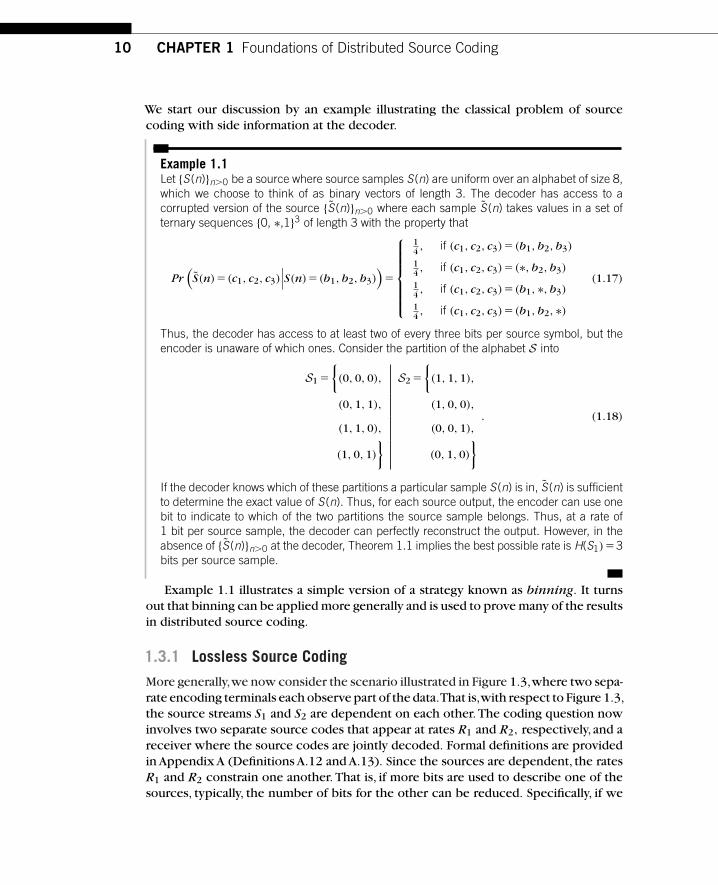
Example 1.1Let {S (n)}n�0 be a source where source samples S (n) are uniform over an alphabet of size 8,which we choose to think of as binary vectors of length 3. The decoder has access to acorrupted version of the source {S (n)}n�0 where each sample S (n) takes values in a set ofternary sequences {0, ∗,1}3 of length 3 with the property that
Pr(S(n)�(c1, c2, c3)
∣∣∣S(n)�(b1, b2, b3))
�
⎧⎪⎪⎪⎪⎪⎨⎪⎪⎪⎪⎪⎩
14 , if (c1, c2, c3)�(b1, b2, b3)
14 , if (c1, c2, c3)�(∗, b2, b3)
14 , if (c1, c2, c3)�(b1, ∗, b3)
14 , if (c1, c2, c3)�(b1, b2, ∗)
(1.17)
Thus, the decoder has access to at least two of every three bits per source symbol, but theencoder is unaware of which ones. Consider the partition of the alphabet S into
S1 �
{(0, 0, 0), S2 �
{(1, 1, 1),
(0, 1, 1), (1, 0, 0),
(1, 1, 0), (0, 0, 1),
(1, 0, 1)
}(0, 1, 0)
} . (1.18)
If the decoder knows which of these partitions a particular sample S (n) is in, S (n) is sufficientto determine the exact value of S (n). Thus, for each source output, the encoder can use onebit to indicate to which of the two partitions the source sample belongs. Thus, at a rate of1 bit per source sample, the decoder can perfectly reconstruct the output. However, in theabsence of {S (n)}n�0 at the decoder, Theorem 1.1 implies the best possible rate is H(S1)�3bits per source sample.
Example 1.1 illustrates a simple version of a strategy known as binning. It turnsout that binning can be applied more generally and is used to prove many of the resultsin distributed source coding.
1.3.1 Lossless Source Coding
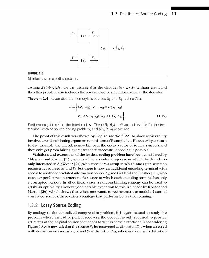
More generally,we now consider the scenario illustrated in Figure 1.3,where two sepa-rate encoding terminals each observe part of the data.That is,with respect to Figure 1.3,the source streams S1 and S2 are dependent on each other. The coding question nowinvolves two separate source codes that appear at rates R1 and R2, respectively, and areceiver where the source codes are jointly decoded. Formal definitions are providedin Appendix A (Definitions A.12 and A.13). Since the sources are dependent, the ratesR1 and R2 constrain one another. That is, if more bits are used to describe one of thesources, typically, the number of bits for the other can be reduced. Specifically, if we
1.3 Distributed Source Coding 11
ˆ ˆ
S 2R 2
S 1
S 1, S 2
R 1ENC
ENC
DEC
FIGURE 1.3
Distributed source coding problem.
assume R2 � log |S2|, we can assume that the decoder knows S2 without error, andthus this problem also includes the special case of side information at the decoder.
Theorem 1.4. Given discrete memoryless sources S1 and S2, define R as
R�
{(R1, R2) :R1 �R2 �H(S1, S2),
R1 �H(S1|S2), R2 �H(S2|S1)
}. (1.19)
Furthermore, let R0 be the interior of R. Then (R1,R2)∈R0 are achievable for the two-terminal lossless source coding problem, and (R1,R2) /∈R are not.
The proof of this result was shown by Slepian and Wolf [22]; to show achievabilityinvolves a random binning argument reminiscent of Example 1.1. However,by contrastto that example, the encoders now bin over the entire vector of source symbols, andthey only get probabilistic guarantees that successful decoding is possible.
Variations and extensions of the lossless coding problem have been considered byAhlswede and Körner [23],who examine a similar setup case in which the decoder isonly interested in S1;Wyner [24], who considers a setup in which one again wants toreconstruct sources S1 and S2, but there is now an additional encoding terminal withaccess to another correlated information source S3;and Gel’fand and Pinsker [25],whoconsider perfect reconstruction of a source to which each encoding terminal has onlya corrupted version. In all of these cases, a random binning strategy can be used toestablish optimality. However,one notable exception to this is a paper by Körner andMarton [26], which shows that when one wants to reconstruct the modulo-2 sum ofcorrelated sources, there exists a strategy that performs better than binning.
1.3.2 Lossy Source Coding
By analogy to the centralized compression problem, it is again natural to study theproblem where instead of perfect recovery, the decoder is only required to provideestimates of the original source sequences to within some distortions. ReconsideringFigure 1.3,we now ask that the source S1 be recovered at distortion D1, when assessedwith distortion measure d1(·, ·), and S2 at distortion D2, when assessed with distortion

12 CHAPTER 1 Foundations of Distributed Source Coding
measure d2(·, ·). The question is again to determine the necessary rates, R1 and R2,
respectively, as well as the coding schemes that permit satisfying the distortion con-straints. Formal definitions are provided in Appendix A (Definitions A.14 and A.15).For this problem,a natural achievable strategy arises. One can first quantize the sourcesat each encoder as in the centralized lossy coding case and then bin the quantized val-ues as in the distributed lossless case. The work of Berger and Tung [27–29] providesan elegant way to combine these two techniques that leads to the following result.The result was independently discovered by Housewright [30].
Theorem 1.5: “Quantize-and-bin.” Given sources S1 and S2 with distortion functions dk :Sk �Uk→��, k∈{1, 2}, the achievable rate-distortion region includes the following set:
R� {(�R, �D) :∃U1, U2 s.t. U1 �S1 �S2 �U2,
E[d1(S1, U1)]D1, E[d2(S2, U2)]D2, (1.20)
R1 � I(S1;U1|U2), R2 � I(S2;U2|U1),
R1 �R2 � I(S1, S2;U1U2)}.A proof for the setting of more than two users is given by Han and Kobayashi
[31,Theorem 1, pp. 280–284]. A major open question stems from the optimality ofthe “quantize-and-bin” achievable strategy. While work by Servetto [32] suggests itmay be tight for the two-user setting, the only case for which it is known is thequadratic Gaussian setting, which is based on an outer bound developed by Wagnerand Anantharam [33, 34].
Theorem 1.6: Wagner, Tavildar, and Viswanath [35]. Given sources S1 and S2 that arejointly Gaussian and i.i.d. in time, that is,
(S1(k),S2(k)
)∼N (0,), with covariance matrix
�
(�2
1 �1�2
�1�2 �22
)(1.21)
for D1, D2 �0 define R(D1,D2) as
R(D1, D2)�
{(R1, R2) :R1 �
1
2log� (1�2 �22�2R2)�2
1
D1,
R2 �1
2log� (1�2 �22�2R1)�2
2
D2,
R1 �R2 �1
2log� (1�2)�2
1�22(D1, D2)
2D1D2
}, (1.22)
where
(D1, D2)�1�
√1�
42D1D2
(1�2)2�21�2
2
. (1.23)
Furthermore, let R0 be the interior of R. Then for distortions D1, D2 �0, (R1, R2)∈R0(D1, D2) are achievable for the two-terminal quadratic Gaussian source codingproblem and (R1, R2) /∈R(D1, D2) are not.

1.3 Distributed Source Coding 13
ˆ
S 2
S 1
S 1
R 1ENC
DEC
FIGURE 1.4
The Wyner–Ziv source coding problem.
In some settings,the rates given by the“quantize-and-bin”achievable strategy can beshown to be optimal. For instance, consider the setting in which the second encoderhas an unconstrained rate link to the decoder, as in Figure 1.4. This configuration isoften referred to as the Wyner–Ziv source coding problem.
Theorem 1.7. Given a discrete memoryless source S1, discrete memoryless side informa-tion source S2 with the property that (S1(k),S2(k)) are i.i.d. over k, and bounded distortionfunction d : S �U→��, a rate R is achievable with lossy source coding with side informationat the decoder and with distortion D if R � RWZ
S1|S2(D). Here
RWZS1|S2
(D)� minp(u|s):
U�S1�S2E[d(S1,U )]D
I(S1;U |S2) (1.24)
is the rate distortion function for side information at the decoder. Conversely, forR � RWZ
S1|S2(D), the rate R is not achievable with distortion D.
Theorem 1.7 was first proved by Wyner and Ziv [36]. An accessible summary ofthe proof is given in [3,Theorem 14.9.1, pp. 438–443].
The result can be extended to continuous sources and unbounded distortion mea-sures under appropriate regularity conditions [37]. It turns out that for the quadraticGaussian case, that is, jointly Gaussian source and side information with a mean-squared error distortion function, these regularity conditions hold, and one can char-acterize the achievable rates as follows. Note the correspondence between this resultand Theorem 1.6 as R2→�.
Proposition 1.3. Consider a source S1 and side information source S2 such that(S1(k), S2(k))∼N (0, ) are i.i.d. in k, with
��2(
1 1
)(1.25)
Then for distortion function d(s1, u)�(s1 �u)2 and for D �0,
RWZS1|S2
(D)�1
2log� (1�2)�2
D. (1.26)
14 CHAPTER 1 Foundations of Distributed Source Coding
1.3.2.1 Rate LossInterestingly, in this Gaussian case,even if the encoder in Figure 1.4 also had access tothe source X2 as in the conditional rate-distortion problem,the rate-distortion functionwould still be given by Proposition 1.3. Generally, however, there is a penalty for theabsence of the side information at the encoder. A result of Zamir [38] has shown thatfor memoryless sources with finite variance and a mean-squared error distortion, therate-distortion function provided in Theorem 1.7 can be no larger than 1
2 bit/sourcesample than the rate-distortion function given in Theorem 1.3.
It turns out that this principle holds more generally. For centralized source codingof a length M zero-mean vector Gaussian source {�S(n)}n�0 with covariance matrixS having diagonal entries �2
S and eigenvalues �(M)1 , . . . , �
(M)M with the property that
�(M)m �� for some � �0 and all m, and squared error distortion, the rate-distortion
function is given by [10]
R�S(D)�
M∑m�1
1
2log
�m
Dm, (1.27)
Dm �
{� � ��m,
�m otherwise,(1.28)
where∑M
m�1 Dm �D. Furthermore, it can be lower bouned by [39]
R�S(D)�M
2log
M�
D. (1.29)
Suppose each component {Sm(n)}n�0 were at a separate encoding terminal.Thenit is possible to show that by simply quantizing, without binning, an upper bound onthe sum rate for a distortion D is given by [39]
M∑m�1
Rm M
2log
(1�
M�2S
D
). (1.30)
Thus, the scaling behavior of (1.27) and (1.30) is the same with respect to both smallD and large M .
1.3.2.2 Optimality of “Quantize-and-bin” StrategiesIn addition toTheorems 1.6 and 1.7,“quantize-and-bin”strategies have been shown tobe optimal for several special cases,some of which are included in the results of Kaspiand Berger [40]; Berger and Yeung [41]; Gastpar [42]; and Oohama [43].
By contrast, “quantize-and-bin” strategies have been shown to be strictly subop-timal. Analogous to Körner and Marton’s result in the lossless setting [26], work byKrithivasan and Pradhan [44] has shown that rate points outside those prescribed bythe “quantize-and-bin” achievable strategy are achievable by exploiting the structureof the sources for multiterminal Gaussian source coding when there are more thantwo sources.

1.3 Distributed Source Coding 15
1.3.2.3 Multiple Descriptions ProblemMost of the problems discussed so far have assumed a centralized decoder with accessto encoded observations from all the encoders. A more general model could alsoinclude multiple decoders, each with access to only some subset of the encodedobservations.While little is known about the general case,considerable effort has beendevoted to studying the multiple descriptions problem.This refers to the specific caseof a centralized encoder that can encode the source more than once, with subsetsof these different encodings available at different encoders. As in the case of thedistributed lossy source coding problem above, results for several special cases havebeen established [45–55].
1.3.3 Interaction
Consider Figure 1.5,which illustrates a setting in which the decoder has the ability tocommunicate with the encoder and is interested in reconstructing S. Seminal workby Orlitsky [56,57] suggests that under an appropriate assumption,the benefits of thiskind of interaction can be quite significant. The setup assumes two random variablesS and U with a joint distribution, one available at the encoder and the other at thedecoder. The decoder wants to determine S with zero probability of error, and thegoal is to minimize the total number of bits used over all realizations of S and U withpositive probability. The following example illustrates the potential gain.
Example 1.2(The League Problem [56]) Let S be uniformly distributed among one of 2m teams in asoftball league. S corresponds to the winner of a particular game and is known to the encoder.The decoder knows U, which corresponds to the two teams that played in the tournament.Since the encoder does not know the other competitor in the game, if the decoder cannotcommunicate with the encoder, the encoder must send m bits in order for the decoder todetermine the winner with zero probability of error.
Now suppose the decoder has the ability to communicate with the encoder. It can simplylook for the first position at which their binary expansion differs and request that from theencoder. This request costs log2 m bits since the decoder simply needs to send one of the mdifferent positions. Finally, the encoder simply sends the value of S at this position, which costsan additional 1 bit. The upshot is that as m gets larger, the noninteractive strategy requiresexponentially more bits than the interactive one.
SENC DEC
S
U
FIGURE 1.5
Interactive source coding.
16 CHAPTER 1 Foundations of Distributed Source Coding
1.4 REMOTE SOURCE CODINGIn many of the most interesting source coding scenarios, the encoders do not getto observe directly the information that is of interest to the decoder. Rather, theymay observe a noisy function thereof. This occurs, for example, in camera and sensornetworks. We will refer to such source coding problems as remote source coding. Inthis section, we discuss two main insights related to remote source coding:
1. For the centralized setting,direct and remote source coding are the same thing,except with respect to different distortion measures (see Theorem 1.8).
2. For the distributed setting, how severe is the penalty of distributed codingversus centralized? For direct source coding, one can show that the penalty isoften small. However, for remote source coding, the penalty can be dramatic(see Equation (1.47)).
The remote source coding problem was initially studied by Dobrushin andTsybakov [58]. Wolf and Ziv explored a version of the problem with a quadratic dis-tortion, in which the source is corrupted by additive noise, and found an elegantdecoupling between estimating the noisy source and compressing the estimate [59].The problem was also studied by Witsenhausen [60].
We first consider the centralized version of the problem before moving on to thedistributed setting. For simplicity, we will focus on the case in which the source andobservation processes are memoryless.
1.4.1 Centralized
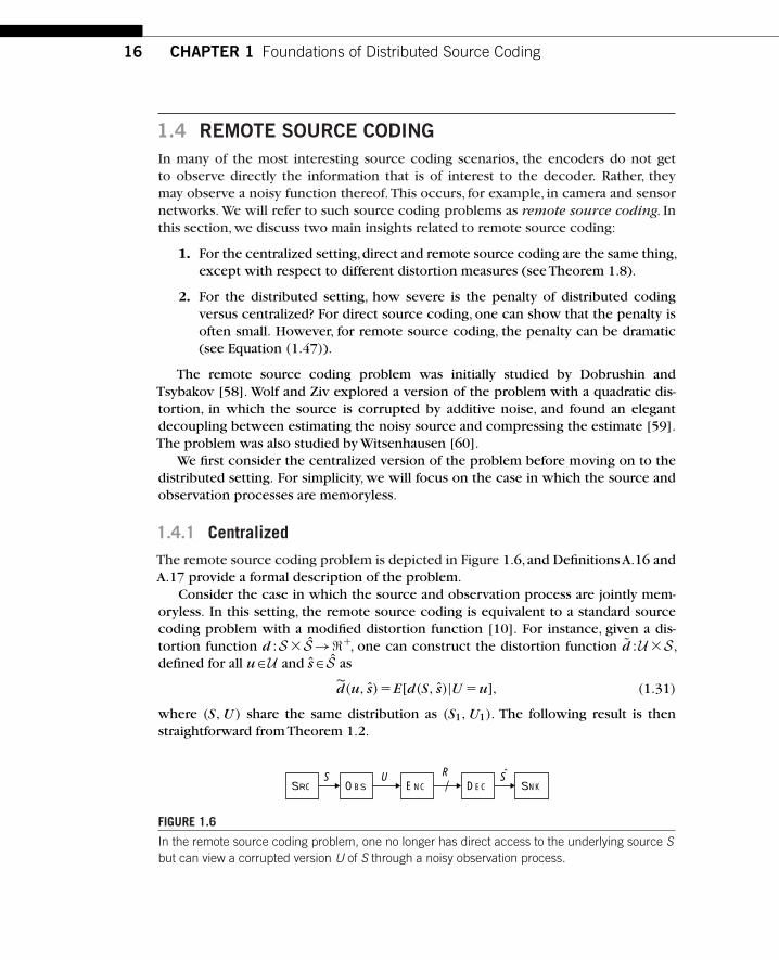
The remote source coding problem is depicted in Figure 1.6, and Definitions A.16 andA.17 provide a formal description of the problem.
Consider the case in which the source and observation process are jointly mem-oryless. In this setting, the remote source coding is equivalent to a standard sourcecoding problem with a modified distortion function [10]. For instance, given a dis-tortion function d :S � S→��, one can construct the distortion function d :U �S,defined for all u∈U and s∈ S as
d(u, s)�E[d(S, s)|U �u], (1.31)
where (S, U ) share the same distribution as (S1, U1). The following result is thenstraightforward from Theorem 1.2.
ˆS U R SENCOBSSRC DEC SNK
FIGURE 1.6
In the remote source coding problem, one no longer has direct access to the underlying source Sbut can view a corrupted version U of S through a noisy observation process.

1.4 Remote Source Coding 17
Theorem 1.8: Remote rate-distortion theorem [10]. Given a discrete memoryless sourceS, bounded distortion function d :S � S→��, and observations U such that
(S(k),U(k)
)are i.i.d. in k, the remote rate-distortion function is
RremoteS (D)� min
p(s|u):S�U�SE[d(S,S)]D
I(U ; S). (1.32)
This theorem extends to continuous sources under suitable regularity conditions,which are satisfied by finite-variance sources under a squared error distortion.
Theorem 1.9: Additive remote rate-distortion bounds. For a memoryless source S, boundeddistortion function d : S � S→��, and observations Ui �Si �Wi, where Wi is a sequenceof i.i.d. random variables,
1
2log
QV
D �D0Rremote
S (D)1
2log
�2V
D �D0, (1.33)
where V�E [S|U ], and D0 �E(S�V )2, and where
QSQW
QUD0
�2S �2
W
�2U
. (1.34)
This theorem does not seem to appear in the literature, but it follows in a relativelystraightforward fashion by combining the results of Wolf and Ziv [59] with Shannon’supper and lower bounds. In addition, for the case of a Gaussian source S and Gaussianobservation noise W , the bounds in both (1.33) and (1.34) are tight. This can beverified using Table 1.1.
Let us next consider the remote rate-distortion problem in which the encodermakes M �1 observations of each source sample. The goal is to illustrate the depen-dence of the remote rate-distortion function on the number of observations M .
To keep things simple, we restrict attention to the scenario shown in Figure 1.7.
ENC DECS S
W 1
U 1
W 2
U 2
W M
U M
R
FIGURE 1.7
An additive remote source coding problem with M observations.

18 CHAPTER 1 Foundations of Distributed Source Coding
More precisely, we suppose that S is a memoryless source and that the observationprocess is
Um(k)�S(k)�Wm(k), k�1, (1.35)
where Wm(k) are i.i.d. (both in k and in m) Gaussian random variables of mean zeroand variance �2
Wm. For this special case, it can be shown [61, Lemma 2] that for any
given time k, we can collapse all M observations into a single equivalent observation,characterized by
U (k)�1
M
M∑m�1
�2W
�2Wm
Um(k) (1.36)
�S(k)�1
M
M∑m�1
�2W
�2Wm
Wm(k), (1.37)
where �2W �
(1M
∑Mm�1
1�2
Wm
)�1
. This works because U (k) is a sufficient statistic for
S(k) given U1(k), . . . , UM (k). However, at this point, we can use Theorem 1.9 toobtain upper and lower bounds on the remote rate-distortion function. For exam-ple, using (1.34), we can observe that as long as the source S satisfies h(S)���, D0
scales linearly with �2W , and thus, inversely proportional to M .
When the source is Gaussian, a precise characterization exists. In particular, Equa-tions (1.33) and (1.34) allow one to conclude that the rate-distortion function is givenby the following result.
Proposition 1.4. Given a memoryless Gaussian source S with S(i)∼N (0, �2S ),
squared error distortion, and the M observations corrupted by an additiveGaussian noise model and given by Equation (1.35), the remote rate-distortionfunction is
RremoteS (D)�
1
2log
�2S
D�
1
2log
�2S
�2U �
�2W �2
SMD
, (1.38)
where
�2U ��2
S ��2
W
Mand �2
W �1
1M
∑Mm�1
1�2
Wm
. (1.39)
As in the case of direct source coding, there is an analogous result for the case ofjointly stationary ergodic Gaussian sources and observations.
Proposition 1.5. Let S be a stationary ergodic Gaussian source S, U an observationprocess that is jointly stationary ergodic Gaussian with S, and �S(�), �U (�), and
1.4 Remote Source Coding 19
�S,U (�) be their corresponding power and cross spectral densities.Then for mean-squared error distortion, the remote rate-distortion function is given by
RremoteS (D�)�
1
4�
∫ �
��max
{0,|�S,U (�)|2
��U (�)
}d� (1.40)
D� �1
2�
∫ �
��
(�S(�)�U (�)� |�S,U (�)|2
�U (�)
)d�
�1
2�
∫ �
��min
{�,|�S,U (�)|2
�U (�)
}d�. (1.41)
PROOF. See Berger [10, pp. 124–129]. ■
Observe that 12�
∫ ���
(�S(�)�U (�)�|�S,U (�)|2
�U (�)
)d� is simply the mean-squared error
resulting from applying a Wiener filter on U to estimate S.
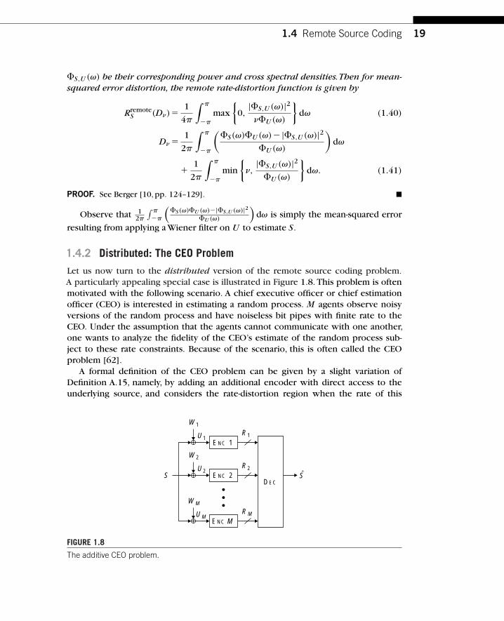
1.4.2 Distributed: The CEO Problem
Let us now turn to the distributed version of the remote source coding problem.A particularly appealing special case is illustrated in Figure 1.8. This problem is oftenmotivated with the following scenario. A chief executive officer or chief estimationofficer (CEO) is interested in estimating a random process. M agents observe noisyversions of the random process and have noiseless bit pipes with finite rate to theCEO. Under the assumption that the agents cannot communicate with one another,one wants to analyze the fidelity of the CEO’s estimate of the random process sub-ject to these rate constraints. Because of the scenario, this is often called the CEOproblem [62].
A formal definition of the CEO problem can be given by a slight variation ofDefinition A.15, namely, by adding an additional encoder with direct access to theunderlying source, and considers the rate-distortion region when the rate of this
ENC 1
ENC 2
ENC M
DECS S
W 1
U 1R 1
W 2
U 2R 2
W M
U MR M
FIGURE 1.8
The additive CEO problem.

20 CHAPTER 1 Foundations of Distributed Source Coding
encoder is set to zero. The formal relationship is established in Definitions A.18and A.19.
The CEO problem has been used as a model for sensor networks, where theencoders correspond to the sensors, each with access to a noisy observation of somestate of nature. Unfortunately (and perhaps not too surprisingly), the general CEOproblem remains open. On the positive side, the so-called quadratic Gaussian CEOproblem has been completely solved. Here, with respect to Figure 1.8, the source Sis a memoryless Gaussian source, and the noises Wm(k) are i.i.d. (both in k and inm) Gaussian random variables of mean zero and variance �2
Wm. The setting was first
considered by Viswanathan and Berger [63], and later refined (see, e.g. [43, 64, 65] or[66, 67]), leading to the following theorem:
Theorem 1.10. Given a memoryless Gaussian source S with S(i )∼N (0,�2S), squared error
distortion, and the M observations corrupted by an additive Gaussian noise model and givenby Equation (1.35), and assume that �2
W1�2
W2 · · ·�2
WM. Then the sum rate-distortion
function for the CEO problem is given by
RCEOS (D)�
1
2log
�2S
D�
1
2log
(K∏
m�1
�2Wm
)�
K
2log
(1
KDK�
1
KD
), (1.42)
where K is the largest integer in {1, . . . ,M } satisfying
1
D�
1
�2S
��K �1
�2WK
�
K�1∑m�1
1
�2Wm
(1.43)
and
1
DK�
1
�2S
�
K∑m�1
1
�2Wm
. (1.44)
Furthermore, if �2Wm
��2W for all m�1, . . . , M ,
RCEOS (D)�
1
2log
�2S
D�
M
2log
�2S
�2U �
�2W �2
SMD
, (1.45)
where
�2U ��2
S ��2
W
M. (1.46)
Alternate strategies for achieving the sum rate have been explored [68] and achievablestrategies for the case of vector-Gaussian sources have been studied [69, 70], but therate region for this setting remains open.
We conclude this section by discussing the rate loss between the joint remotesource coding problem (illustrated in Figure 1.7) and the distributed remote sourcecoding problem (illustrated in Figure 1.8). For the quadratic Gaussian scenario with
1.4 Remote Source Coding 21
equal noise variances �2Wm
��2W , this rate loss is exactly characterized by comparing
Proposition 1.4 with Theorem 1.10, leading to
RCEOS (D)�Rremote
S (D)�M �1
2log
�2S
�2S �
�2W
M (1��2
SD )
. (1.47)
By letting M→�, this becomes
RCEOS (D)�Rremote
S (D)��2
W
2
(1
D�
1
�2S
), (1.48)
so the rate loss scales inversely with the target distortion. Note that this behavior isdramatically different from the one found in Section 1.3.2.1;as we have seen there, fordirect source coding,both centralized and distributed encoding have the same scalinglaw behavior with respect to large M and small D (at least under the assumptionsstated in Section 1.3.2.1). By contrast, as the quadratic Gaussian example reveals, forremote source coding, centralized and distributed encoding can have very differentscaling behaviors.
It turns out that the quadratic Gaussian example has the worst case rate lossbehavior among all problems that involve additive Gaussian observation noise andmean-squared error distortion (but arbitrary statistics of the source S). More precisely,we have the following proposition, proved in [61]:
Proposition 1.6. Given a real-valued zero-mean memoryless source S with variance�2
S , squared error distortion, and the M observations corrupted by an additiveGaussian noise model and given by Equation (1.35) with �2
Wi��2
W , the differencebetween the sum rate-distortion function for the CEO problem and the remote rate-distortion function is no more than
RCEOS (D)�Rremote
S (D) M �1
2log
�2S
�2S �
�2W
M (1��2
SD )
�1
2log
(M�1)D�2W ��2
S (M(2D�2√
D�2W )�MD(D�2
√D�2
W ))
D(M�2S ��2
W )��2W �2
S. (1.49)
By letting M→�, this becomes
RCEOS (D)�Rremote
S (D)�2
W
2
(1
D�
1
�2S
)�
1
2log
(1�
(1
D�
1
�2S
)(D �2
√D�2
W )
).
(1.50)
Thus, the rate loss cannot scale more than inversely with the distortion D evenfor non-Gaussian sources. Bounds for the rate loss have been used to give tighterachievable bounds for the sum rate when the source is non-Gaussian [71].
Although the gap between distributed and centralized source coding of a remotesource can be significant,cooperative interaction among the encoders can potentiallydecrease the gap. While this has been studied when the source is Gaussian [72], thequestion remains open for general sources.
22 CHAPTER 1 Foundations of Distributed Source Coding
1.5 JOINT SOURCE-CHANNEL CODINGWhen information is to be stored on a perfect (error-free) discrete (e.g., binary)medium, then the source coding problem surveyed in this chapter is automaticallyrelevant. However, in many tasks, the source information is compressed because itmust be communicated across a noisy channel.There, it is not evident that the formal-izations discussed in this chapter are relevant. For the stationary ergodic point-to-pointproblem,Shannon’s separation theorem proves that,indeed,an optimal architecture isto first compress the source information down to the capacity of the channel,and thencommunicate the resulting encoded bit stream across the noisy channel in a reliablefashion.
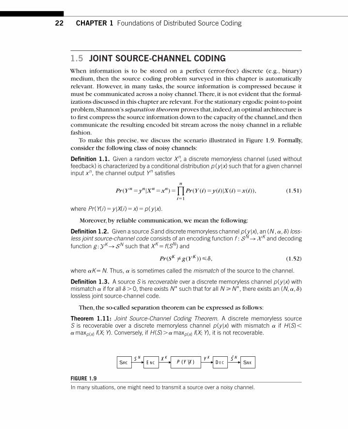
To make this precise, we discuss the scenario illustrated in Figure 1.9. Formally,consider the following class of noisy channels:
Definition 1.1. Given a random vector Xn, a discrete memoryless channel (used withoutfeedback) is characterized by a conditional distribution p (y |x) such that for a given channelinput xn, the channel output Yn satisfies
Pr(Y n �yn|Xn �xn)�
n∏i�1
Pr(Y (i)�y(i)|X(i)�x(i)), (1.51)
where Pr (Y(i )�y |X(i )�x)�p (y |x).
Moreover, by reliable communication, we mean the following:
Definition 1.2. Given a source S and discrete memoryless channel p (y |x), an (N , �, ) loss-less joint source-channel code consists of an encoding function f : SN→X K and decodingfunction g : YK→SN such that XK � f (SN) and
Pr(SK ��g(Y K )) , (1.52)
where �K�N. Thus, � is sometimes called the mismatch of the source to the channel.
Definition 1.3. A source S is recoverable over a discrete memoryless channel p (y |x) withmismatch � if for all � 0, there exists N∗ such that for all N �N∗, there exists an (N, �, )
lossless joint source-channel code.
Then, the so-called separation theorem can be expressed as follows:
Theorem 1.11: Joint Source-Channel Coding Theorem. A discrete memoryless sourceS is recoverable over a discrete memoryless channel p (y |x) with mismatch � if H (S)�� maxp(x) I(X; Y). Conversely, if H (S)�� maxp(x) I(X; Y), it is not recoverable.
ENC P (Y |X )SRC DEC SNKS
N S
NX
K Y
K
FIGURE 1.9
In many situations, one might need to transmit a source over a noisy channel.

A.1 Notation 23
A proof of this theorem can be found, for example, in [3]. One should note that The-orem 1.11 can be stated more generally for both a larger class of sources and forchannels.
The crux, however, is that there is no equivalent of the separation theorem incommunication networks.One of the earliest examples of this fact was given by [73]:when correlated sources are transmitted in a lossless fashion across a multiple-accesschannel, it is not generally optimal to first compress the sources with the Slepian–Wolf code discussed in Section 1.3,thus obtaining smaller and essentially independentsource descriptions,and sending these descriptions across the multiple-access channelusing a capacity-approaching code. Rather, the source correlation can be exploited toaccess dependent input distributions on the multiple-access channels, thus enlargingthe region of attainable performance. A more dramatic example was found in [74–76]. In that example,modeling a simple“sensor”network,a single underlying source isobserved by M terminals subject to independent noises.These terminals communicateover an additive multiple-access channel to a “fusion center” whose only goal is torecover the single underlying source to within the smallest squared error. For thisproblem, one may use the CEO source code discussed in Section 1.4.2, followed by aregular capacity-approaching code for the multiple-access channel.Then, the smallestsquared error distortion D decreases like 1/ log M . However, it can be shown thatthe optimal performance for a joint source-channel code decreases like 1/M, thatis, exponentially better. For some simple instances of the problem, the optimal jointsource-channel code is simply uncoded transmission of the noisy observations [77].Nevertheless, for certain classes of networks, one can show that a distributed sourcecode followed by a regular channel code is good enough, thus establishing partialand approximate versions of network separation theorems. An account of this can befound in [78].
ACKNOWLEDGMENTSThe authors would like to acknowledge anonymous reviewers and others who wentthrough earlier versions of this manuscript. In particular, Mohammad Ali Maddah-Alipointed out and corrected an error in the statement of Theorem 1.10.
APPENDIX A: Formal Definitions and NotationsThis appendix contains technical definitions that will be useful in understanding theresults in this chapter.
A.1 NOTATIONUnless otherwise stated, capital letters X, Y , Z denote random variables, lower-caseletters x, y, z instances of these random variables,and calligraphic letters X , Y, Z sets.
24 CHAPTER 1 Foundations of Distributed Source Coding
The shorthand p(x, y), p(x), and p(y) will be used for the probability distributionsPr(X �x, Y �y), Pr(X �x), and Pr(Y �y). XN will be used to denote the randomvector X1, X2, . . . , XN .The alternate vector notation �R and �D will sometimes be used torepresent achievable rate-distortion regions. Finally,we will use the notation X �Y �Zto denote that the random variables X, Y , Z form a Markov chain.That is,X and Z areindependent given Y .
We start by defining the notion of entropy, which will be useful in the sequel.
Definition A.1. Let X,Y be discrete random variables with joint distribution p (x, y ). Thenthe entropy H (X ) of X is a real number given by the expression
H(X)��E[log p(X)]��∑
x
p(x) log p(x), (A.53)
the joint entropy H (X,Y ) of X and Y is a real number given by the expression
H(X, Y )��E[log p(X, Y )]��∑x,y
p(x, y) log p(x, y), (A.54)
and the conditional entropy H (X|Y ) of X given Y is a real number given by the expression
H(X |Y )��E[log p(X |Y )]�H(X, Y )�H(Y ). (A.55)
With a definition for entropy, we can now define mutual information.
Definition A.2. Let X, Y be discrete random variables with joint distribution p (x, y).Then the mutual information I (X; Y ) between X and Y is a real number given by theexpression
I(X;Y )�H(X)�H(X |Y )�H(Y )�H(Y |X). (A.56)
Similar definitions exist in the continuous setting.
Definition A.3. Let X, Y be continuous random variables with joint density f (x, y). Thenwe define the differential entropy h (X )��E [log f (X )], joint differential entropy h (X,Y )��E [log f (X,Y )], conditional differential entropy h (X |Y )��E [log f (X |Y )], and mutual infor-mation I (X; Y )�h (X )�h (X |Y )�h (Y )�h (Y |X ).
Definition A.4. Let X be a continuous random variable with density f (x). Then its entropypower QX is given by
QX �1
2�eexp{2h(X)}. (A.57)
The central concept in this chapter is the information source, which is merely adiscrete-time random process {S(n)}n�0. For the purposes of this chapter, we assumethat all information sources are stationary and ergodic. When the random variables{S(n)}n�0 take values in a discrete set, we will refer to the source as a discrete infor-mation source. For simplicity,we will refer to a source {S(n)}n�0 with the abbreviatednotation S.

A.1 Notation 25
Definition A.5. The entropy rate of a stationary and ergodic discrete information sourceS is
H�(S)� limn→�
1
nH(S(1), S(2), . . . , S(n))� lim
n→�H(S(n)|S(n�1), S(n�2), . . . , S(1)).
(A.58)
In many of the concrete examples discussed in this chapter,S will be assumed to bea sequence of independent and identically distributed (i.i.d.) random variables.This isusually referred to as a memoryless source, and one can show that H�(S)�H (S(1)).For notational convenience, we will denote this simply as H(S).
A.1.1 Centralized Source CodingDefinition A.6. Given a source S, an (N, R, ) lossless source code consists of an encodingfunction f : SN→{1, . . . , M} and decoding function g : {1, . . . , M}→SN such that
Pr(SN ��g
(f (SN )
)) , (A.59)
where M�2NR.
In the above definition, R has units in bits per source sample. Thus, R is oftenreferred to as the rate of the source code.
Definition A.7. Given a source S, a rate R is achievable via lossless source coding if forall �0, there exists N∗ such that for N�N∗, there exists an (N, R� , ) lossless sourcecode.
Similarly, definitions can be given in the lossy case.
Definition A.8. Given a source S and distortion function d : S � S→��, an (N, R, D) cen-tralized lossy source code consists of an encoding function f : SN→{1, . . . ,M} and decoding
function g : {1, . . . ,M}→ SN such that for SN
�g(f (SN)
)N∑
i�1
E[d(S(i), S(i))]ND, (A.60)
where M = 2 NR .
Definition A.9. Given a source S and distortion function d : S � S→R�, a rate R is achiev-
able with distortion D if for all �0, there exists a sequence of (N, RN, DN) centralized lossysource codes and N∗ such that for N�N∗, RN �R� , DN D� .
Definition A.10. Given a source S1, source side information S2 available at the encoderand decoder, and distortion function d : S1 � S1→��, an (N, R, D) conditional lossy sourcecode consists of an encoding function f : SN
1 �SN2 →{1, . . . ,M} and decoding function
g : {1, . . . ,M}�SN2 → SN
1 such that for SN1 �g
(f (SN
1 ,SN2 ),SN
2
),
N∑i�1
E[d(S(i), S(i))]ND, (A.61)
where M�2NR.
26 CHAPTER 1 Foundations of Distributed Source Coding
Definition A.11. Given a source S1, source side information S2 available at the encoderand decoder, and distortion function d : S1 � S1→��, a rate R is achievable with distortionD if for all �0, there exists a sequence of (N, RN ,DN) conditional lossy source codes andN∗ such that for N � N∗, RN � R� , DN D� . The supremum over all achievable R isthe conditional rate-distortion function, denoted as RS1|S2 (D).
A.1.2 Distributed Source Coding
We first consider the lossless case.
Definition A.12. Given discrete sources S1 and S2, an (N,R1,R2, ) two-terminal loss-less source code consists of two encoding functions f1 :SN
1 →{1, . . . ,M1} and f2 :SN2 →
{1, . . . ,M2} as well as a decoding function g : {1, . . . ,M1}�{1, . . . ,M2}→SN1 �SN
2 suchthat
Pr((SN
1 , SN2 ) ��g
(f1(S
N1 ), f2(S
N2 )))
, (A.62)
where Mi �2NRi .
Definition A.13. Given discrete sources S1 and S2, a rate pair (R1,R2) is achievable forthe two-terminal lossless source coding problem if for all � 0, there exists a sequenceof (N,R1,N, R2, N, N) lossless source codes and N∗ such that for N � N∗, R1,N �R1 � ,R2,N � R2 � , and N .
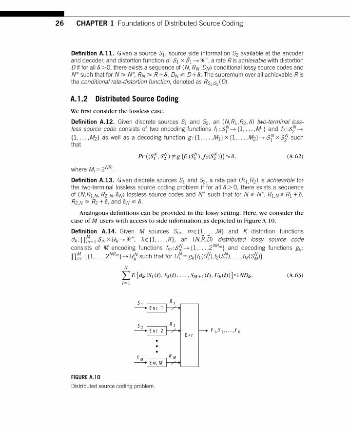
Analogous definitions can be provided in the lossy setting. Here, we consider thecase of M users with access to side information, as depicted in Figure A.10.
Definition A.14. Given M sources Sm, m∈{1, . . . ,M} and K distortion functionsdk :
∏Mm�1 Sm �Uk→��, k∈{1, . . . ,K}, an (N,�R,�D) distributed lossy source code
consists of M encoding functions fm :SNm→{1, . . . ,2NRm} and decoding functions gk :∏M
m�1{1, . . . ,2NRm}→UNk such that for UN
k �gk(f1(SN
1 ),f2(SN2 ), . . . ,fM(SN
M))
N∑i�1
E[dk (S1(i), S2(i), . . . , SM�1(i), Uk(i))
]NDk. (A.63)
DEC
ENC 1
ENC 2
ENCM
R 1
R 2Y 1,Y 2, . . . ,Y K
R M
S 1
S 2
S M
FIGURE A.10
Distributed source coding problem.

A.1 Notation 27
Definition A.15. Given M sources Sm, m∈{1, . . . ,M} and K distortion functions dk :∏Mm�1 Sm �Uk→��, k∈{1, . . . ,K}, a rate-distortion vector (�R, �D) is achievable with a dis-
tributed lossy source code if for all �0, there exists a sequence of (N,�RN,�DN) lossy sourcecodes with side information at the decoder and N∗ such that for all N �N∗, Rm,N �Rm � ,Dk,N Dk � , m∈{1, . . . ,M}, k∈{1, . . . ,K}.
A.1.3 Remote Source Coding
Definition A.16. Given a source S, distortion function d :S � S→��, and observation pro-cess U, an (N,R,D) remote source code consists of an encoding function f : UN→{1, . . . ,M}and decoding function g : {1, . . . ,M}→ SN such that for SN �g
(f (UN)
)N∑
i�1
E[d(S(i), S(i))]ND, (A.64)
where M = 2 NR.
Definition A.17. Given a source S, distortion function d : S �S→��, and observation pro-cess U, a rate R is achievable with distortion D if for all �0, there exists a sequence of(N,RN,DN) remote source codes and N∗ such that for all N � N∗, RN �R� , DN D� .The supremum over all achievable R is the remote rate-distortion function, denoted asR remote
S (D).
The CEO problem is a special case of the distributed source coding problem, asdepicted in Figure A.11.
Definition A.18. Given M�1 sources, S and Um, m∈{1, . . . ,M} and a distortion func-tion d : S � S→��, an (N,�R,D) CEO source code—where �R is a length M vector on the
nonnegative reals—is an M�1 user, single-distortion function, (N, �R,D) distributed lossysource code, where R1 �0, Rm �Rm�1 for m∈{2, . . . ,M�1} S�S1, Um �Sm�1, with thedistortion function d1 :
∏M�1m�1 Sm � S1→�� having the property that
d1(s, u1, . . . , uM , s1)�d(s, s1). (A.65)
DEC
ENC 1
ENC 2
ENC M11
0
R 2
R M
S 1
~
~
S 2
S M 11
S 1DEC
ENC 0
ENC 1
ENC M
0
R 1
R M
S
U 1
U M
S
FIGURE A.11
CEO problem as special case of distributed source coding problem.
28 CHAPTER 1 Foundations of Distributed Source Coding
Definition A.19. Given M�1 sources, S and Um, m∈{1, . . . ,M} and a distortion functiond : S � S→��, a sum rate-distortion pair (R,D) is achievable with a CEO source code if forall �0, there exists a sequence of (N,�RN,DN) CEO source codes and N∗ such that for allN � N∗,
∑Mm�1 Rm,N �R� , DN D� . For a given distortion D, the supremum over R
for all achievable sum rate-distortion pairs (R,D) specifies the sum rate-distortion functionfor the CEO problem, denoted by RCEO
S (D).
REFERENCES[1] C. E. Shannon, “A mathematical theory of communication,” Bell System Technical Journal,
vol. 27, pp. 379–423, 623–656, 1948.
[2] T. S. Han and S. Verdú, “Approximation theory of output statistics,” IEEE Transactions onInformation Theory, vol. 39, no. 3, pp. 752–772, May 1993.
[3] T. Cover and J.Thomas,Elements of Information Theory. NewYork:JohnWiley and Sons,1991.
[4] R. Pilc, “The transmission distortion of a source as a function of the length encoding blocklength,”Bell System Technical Journal, vol. 47, no. 6, pp. 827–885, 1968.
[5] S. Arimoto, “An algorithm for calculating the capacity and rate-distortion functions,” IEEETransactions on Information Theory, vol. 18, pp. 14–20, 1972.
[6] R. Blahut,“Computation of channel capacity and rate-distortion functions,” IEEE Transactionson Information Theory, vol. 18, pp. 460–473, 1972.
[7] K. Rose,“A mapping approach to rate-distortion computation and analysis,” IEEE Transactionson Information Theory, vol. 40, pp. 1939–1952, 1994.
[8] C. Shannon,“Coding theorems for a discrete source with a fidelity criterion,” IRE ConventionRec., vol. 7, pp. 142–163, 1959.
[9] T. Linder and R. Zamir, “On the asymptotic tightness of the Shannon lower bound,” IEEETransactions on Information Theory, pp. 2026–2031, November 1994.
[10] T. Berger, Rate Distortion Theory: A Mathematical Basis for Data Compression, ser.Information and System Sciences Series. Englewood Cliffs, NJ: Prentice-Hall, 1971.
[11] R. Gray,“Conditional rate-distortion theory,”Stanford University,Tech. Rep., October 1972.
[12] J. Omura, “A coding theorem for discrete-time sources,” IEEE Transactions on InformationTheory, vol. 19, pp. 490–498, 1973.
[13] K. Marton,“Error exponent for source coding with a fidelity criterion,” IEEE Transactions onInformation Theory, vol. 20, no. 2, pp. 197–199, March 1974.
[14] A. Wyner and J. Ziv, “Bounds on the rate-distortion function for sources with memory,” IEEETransactions on Information Theory, vol. 17, no. 5, pp. 508–513, September 1971.
[15] R. Gray,“Sliding-block source coding,”IEEE Transactions on Information Theory,vol. 21,no. 4,pp. 357–368, July 1975.
[16] H. Witsenhausen,“On the structure of real-time source coders,”Bell System Technical Journal,vol. 58, no. 6, pp. 1437–1451, 1979.
[17] D. Neuhoff and R. Gilbert,“Causal source codes,” IEEE Transactions on Information Theory,vol. 28, no. 5, pp. 710–713, September 1982.
[18] A. Lapidoth, “On the role of mismatch in rate distortion theory,” IEEE Transactions onInformation Theory, vol. 43, pp. 38–47, January 1997.
[19] A. Dembo and T. Weissman,“The minimax distortion redundancy in noisy source coding,” IEEETransactions on Information Theory, vol. 49, pp. 3020–3030, 2003.

References 29
[20] T.Weissman,“Universally attainable error-exponents for rate-distortion coding of noisy sources,”IEEE Transactions on Information Theory, vol. 50, no. 6, pp. 1229–1246, 2004.
[21] A. Gersho and R. Gray, Vector Quantization and Signal Compression. Boston: KluwerAcademic Publishers, 1992.
[22] D. Slepian and J. Wolf,“Noiseless coding of correlated information sources,” IEEE Transactionson Information Theory, vol. 19, pp. 471–480, 1973.
[23] R. Ahlswede and J. Korner,“Source coding with side information and a converse for degradedbroadcast channels,” IEEE Transactions on Information Theory, vol. 21, no. 6, pp. 629–637,November 1975.
[24] A. Wyner, “On source coding with side information at the decoder,” IEEE Transactions onInformation Theory, vol. 21, no. 3, pp. 294–300, May 1975.
[25] S. Gel’fand and M. Pinsker, “Coding of sources on the basis of observations with incom-plete information (in Russian),” Problemy Peredachi Informatsii (Problems of InformationTransmission), vol. 25, no. 2, pp. 219–221, April–June 1979.
[26] J. Korner and K. Marton,“How to encode the modulo-two sum of binary sources (Corresp.),”IEEE Transactions on Information Theory, vol. 25, no. 2, pp. 219–221, March 1979.
[27] T. Berger and S. Tung, “Encoding of correlated analog sources,” in 1975 IEEE–USSR JointWorkshop on Information Theory. Moscow: IEEE Press, 1975, pp. 7–10.
[28] S. Tung,“Multiterminal source coding,”Ph.D. dissertation, Cornell University, 1977.
[29] T. Berger,“Multiterminal source coding,” in Lecture Notes presented at CISM Summer Schoolon the Information Theory Approach to Communications, 1977.
[30] K. B. Housewright, “Source coding studies for multiterminal systems,” Ph.D. dissertation,University of California, Los Angeles, 1977.
[31] T. S. Han and K. Kobayashi,“A unified achievable rate region for a general class of multiterminalsource coding systems,” IEEE Transactions on Information Theory, pp. 277–288, May 1980.
[32] S. D. Servetto,“Multiterminal source coding with two encoders—I: A computable outer bound,”Arxiv, November 2006. [Online]. Available: http://arxiv.org/abs/cs/0604005v3
[33] A. Wagner and V. Anantharam, “An improved outer bound for the multiterminal source cod-ing problem,” in Proc. IEEE International Symposium on Information Theory, Adelaide,Australia, 2005.
[34] ,“An infeasibility result for the multiterminal source-coding problem,”IEEE Transactionson Information Theory, 2008. [Online]. Available: http://arxiv.org/abs/cs.IT/0511103
[35] A. Wagner, S. Tavildar, and P. Viswanath, “Rate region of the quadratic Gaussian two-encodersource-coding problem,” IEEE Transactions on Information Theory, vol. 54, no. 5, pp.1938–1961, May 2008.
[36] A. Wyner and J. Ziv,“The rate-distortion function for source coding with side information at thedecoder,” IEEE Transactions on Information Theory, vol. 22, pp. 1–10, January 1976.
[37] A.Wyner,“The rate-distortion function for source coding with side information at the decoder—II: General sources,” Information and Control, vol. 38, pp. 60–80, 1978.
[38] R. Zamir,“The rate loss in theWyner–Ziv problem,”IEEE Transactions on Information Theory,vol. 42, pp. 2073–2084, November 1996.
[39] K. Eswaran and M. Gastpar, “On the significance of binning in a scaling-law sense,” inInformation Theory Workshop, Punta del Este, Uruguay, March 2006.
[40] A. H. Kaspi and T. Berger, “Rate-distortion for correlated sources with partially separatedencoders,” IEEE Transactions on Information Theory, vol. IT-28, no. 6, pp. 828–840, 1982.
[41] T. Berger and R. Yeung, “Multiterminal source encoding with one distortion criterion,” IEEETransactions on Information Theory, vol. IT-35, pp. 228–236, 1989.

30 CHAPTER 1 Foundations of Distributed Source Coding
[42] M. Gastpar,“TheWyner–Ziv problem with multiple sources,”IEEETransactions on InformationTheory, vol. 50, no. 11, pp. 2762–2768, November 2004.
[43] Y. Oohama,“Rate-distortion theory for Gaussian multiterminal source coding systems with sev-eral side informations at the decoder,” IEEE Transactions on Information Theory, vol. 51,pp. 2577–2593, 2005.
[44] D. Krithivasan and S. S. Pradhan, “Lattices for distributed source coding: Jointly Gaus-sian sources and reconstruction of a linear function,” Arxiv, July 2007. [Online]. Available:http://arxiv.org/abs/0707.3461
[45] H. Witsenhausen, “On source networks with minimal breakdown degradation,” Bell SystemTechnical Journal, vol. 59, no. 6, pp. 1083–1087, July–August 1980.
[46] , “On team guessing with independent informations,” Math. Oper. Res., vol. 6, no. 2,pp. 293–304, May 1981.
[47] ,“Team guessing with lacunary information,”Math. Oper. Res., vol. 8, no. 1, pp. 110–121,February 1983.
[48] H. Witsenhausen and A. Wyner,“Source coding for multiple descriptions II:A binary source,”Bell System Technical Journal, vol. 60, no. 10, pp. 2281–2292, December 1981.
[49] A. El Gamal and T. Cover, “Achievable rates for multiple descriptions,” IEEE Transactions onInformation Theory, vol. 28, no. 6, pp. 851–857, November 1982.
[50] J. Wolf, A. Wyner, and J. Ziv, “Source coding for multiple descriptions,” Bell System TechnicalJournal, vol. 59, no. 8, pp. 1417–1426, October 1980.
[51] T. Berger and Z. Zhang, “Minimum breakdown degradation in binary source coding,” IEEETransactions on Information Theory, vol. 29, no. 6, pp. 807–814, November 1983.
[52] L. Ozarow,“On a source-coding problem with two channels and three receivers,” Bell SystemTechnical Journal, vol. 59, no. 10, pp. 1909–1921, 1980.
[53] R. Ahlswede,“The rate-distortion region for multiple descriptions without excess rate,” IEEETransactions on Information Theory, vol. 31, no. 6, pp. 721–726, November 1985.
[54] V. Goyal,“Multiple description coding:Compression meets the network,”IEEE Signal ProcessingMagazine, vol. 18, no. 5, pp. 74–93, September 2001.
[55] R. Venkataramani, G. Kramer, and V. Goyal,“Multiple description coding with many channels,”IEEE Transactions on Information Theory, vol. 49, no. 9, pp. 1111–1126, September 2003.
[56] A. Orlitsky,“Worst-case interactive communication I:Two messages are almost optimal,” IEEETransactions on Information Theory, vol. 36, no. 5, pp. 2106–2114, September 1990.
[57] A. Orlitsky, “Worst-case interactive communication II: Two messages are not optimal,” IEEETransactions on Information Theory, vol. 37, no. 4, pp. 995–1005, July 1991.
[58] R. Dobrushin and B. Tsybakov,“Information transmission with additional noise,” IEEE Transac-tions on Information Theory, vol. 8, pp. 293–304, September 1962.
[59] J.Wolf and J. Ziv,“Transmission of noisy information to a noisy receiver with minimum distortion,”IEEE Transactions on Information Theory, vol. 16, pp. 406–411, 1970.
[60] H. Witsenhausen, “Indirect rate distortion problems,” IEEE Transactions on InformationTheory, vol. 26, pp. 518–521, September 1962.
[61] K. Eswaran and M. Gastpar, “Rate loss in the CEO problem,” in 39th Annual Conference onInformation Sciences and Systems, Baltimore, MD, 2005.
[62] T. Berger,Z. Zhang,and H.Viswanathan,“The CEO problem,”IEEE Transactions on InformationTheory, vol. 42, pp. 887–902, May 1996.
[63] H. Viswanathan and T. Berger,“The quadratic Gaussian CEO problem,” IEEE Transactions onInformation Theory, vol. 43, pp. 1549–1559, 1997.

References 31
[64] Y. Oohama, “The rate-distortion function for the quadratic Gaussian CEO problem,” IEEETransactions on Information Theory, vol. 44, pp. 1057–1070, May 1998.
[65] ,“Multiterminal source coding for correlated memoryless Gaussian sources with severalside informations at the decoder,” in Information Theory and Communications Workshop,Proceedings of the 1999 IEEE, South Africa, June 1999.
[66] J. Chen,X. Zhang,T. Berger,and S. B.Wicker,“An upper bound on the sum-rate distortion functionand its corresponding rate allocation schemes for the CEO problem,”IEEE Journal on SelectedAreas in Communications: Special Issue on Sensor Networks, pp. 1–10, 2003.
[67] V. Prabhakaran, D. Tse, and K. Ramchandran, “Rate region of the quadratic Gaussian CEOproblem,” in Proceedings of ISIT, pp. 119-, 2004.
[68] S. C. Draper and G. W. Wornell,“Successively structured CEO problems,”in Proceedings of ISIT,pp. 65-, 2002.
[69] X. Zhang and S. Wicker, “On the rate region of the vector Gaussian CEO problem,” in 39thAnnual Conference on Information Sciences and Systems, Baltimore, MD, 2005.
[70] S. Tavildar and P. Viswanath, “The sum rate for the vector Gaussian CEO problem,” in 2005Asilomar Conference, pp. 3–7, 2005.
[71] K. Eswaran and M. Gastpar,“On the quadratic AWGN CEO problem and non-Gaussian source,”in Proceedings of ISIT, pp. 219–223, 2005.
[72] V. Prabhakaran,K. Ramchandran,and D.Tse,“On the role of interaction between sensors in theCEO problem,”in Annual Allerton Conference on Communication, Control, and Computing,Monticello, IL, October 2004.
[73] T. Cover, A. El Gamal,and M. Salehi,“Multiple access channels with arbitrarily correlated sources,”IEEE Transactions on Information Theory, vol. 26, no. 6, pp. 648–657, November 1980.
[74] M. Gastpar and M. Vetterli,“On the capacity of wireless networks:The relay case,” in Proc. IEEEInfocom 2002, vol. 3, New York, June 2002, pp. 1577–1586.
[75] ,“Source-channel communication in sensor networks,”Information Processing in SensorNetworks, vol. 2, pp. 162–177, 2003.
[76] ,“Power,spatio-temporal bandwidth,and distortion in large sensor networks,”IEEE Jour-nal on Selected Areas in Communications (Special Issue on Self-Organizing DistributiveCollaborative Sensor Networks), vol. 23, no. 4, pp. 745–754, April 2005.
[77] M. Gastpar,“Uncoded transmission is exactly optimal for a simple Gaussian sensor network,”in Proc.2007 Information Theory and ApplicationsWorkshop, San Diego,CA,February 2007.
[78] M. Gastpar, M. Vetterli, and P. L. Dragotti,“Sensing reality and communicating bits:A dangerousliaison,” IEEE Signal Processing Magazine, vol. 23, no. 4, pp. 70–83, July 2006.

CHAPTER
2Distributed Transform Coding
Varit Chaisinthop and Pier Luigi DragottiDepartment of Electrical and Electronic Engineering,
Imperial College London, UK
C H A P T E R C O N T E N T SIntroduction . . . . . . . . . . . . . . . . . . . . . . . . . . . . . . . . . . . . . . . . . . . . . . . . . . . . . . . . . . . . . . . . . . . . . . . . . . . . . . 33Foundations of Centralized TransformCoding . . . . . . . . . . . . . . . . . . . . . . . . . . . . . . . . . . . . . . . . . . . . 35
Transform Coding Overview . . . . . . . . . . . . . . . . . . . . . . . . . . . . . . . . . . . . . . . . . . . . . . . . . . . . . . . . 35Lossless Compression . . . . . . . . . . . . . . . . . . . . . . . . . . . . . . . . . . . . . . . . . . . . . . . . . . . . . . . . . . . . . . 36Quantizers. . . . . . . . . . . . . . . . . . . . . . . . . . . . . . . . . . . . . . . . . . . . . . . . . . . . . . . . . . . . . . . . . . . . . . . . . . 37Bit Allocation . . . . . . . . . . . . . . . . . . . . . . . . . . . . . . . . . . . . . . . . . . . . . . . . . . . . . . . . . . . . . . . . . . . . . . 38Transforms . . . . . . . . . . . . . . . . . . . . . . . . . . . . . . . . . . . . . . . . . . . . . . . . . . . . . . . . . . . . . . . . . . . . . . . . . 39Linear Approximation . . . . . . . . . . . . . . . . . . . . . . . . . . . . . . . . . . . . . . . . . . . . . . . . . . . . . . . . . . . . . . 41
The Distributed Karhunen–Loève Transform .. . . . . . . . . . . . . . . . . . . . . . . . . . . . . . . . . . . . . . . . . . . . 42Problem Statement and Notation . . . . . . . . . . . . . . . . . . . . . . . . . . . . . . . . . . . . . . . . . . . . . . . . . . 43The Two-terminal Scenario . . . . . . . . . . . . . . . . . . . . . . . . . . . . . . . . . . . . . . . . . . . . . . . . . . . . . . . . . 44The Multiterminal Scenario and the Distributed KLT Algorithm .. . . . . . . . . . . . . . . . . . 49
Alternative Transforms . . . . . . . . . . . . . . . . . . . . . . . . . . . . . . . . . . . . . . . . . . . . . . . . . . . . . . . . . . . . . . . . . . . 49Practical Distributed Transform Coding with Side Information. . . . . . . . . . . . . . . . . . . . . 50High-rate Analysis of Source Coding with Side Information at Decoder. . . . . . . . . . . . 50
New Approaches to Distributed Compression with FRI . . . . . . . . . . . . . . . . . . . . . . . . . . . . . . . . . . 51Background on Sampling of 2D FRI Signals . . . . . . . . . . . . . . . . . . . . . . . . . . . . . . . . . . . . . . . 52Detailed Example: Coding Scheme for Translating a Bi-level Polygon . . . . . . . . . . . . . 53
Conclusions . . . . . . . . . . . . . . . . . . . . . . . . . . . . . . . . . . . . . . . . . . . . . . . . . . . . . . . . . . . . . . . . . . . . . . . . . . . . . . 58References . . . . . . . . . . . . . . . . . . . . . . . . . . . . . . . . . . . . . . . . . . . . . . . . . . . . . . . . . . . . . . . . . . . . . . . . . . . . . . . 58
2.1 INTRODUCTIONCompression or approximation of an observed source is a central problem in signalprocessing and communications, and transform coding has over the years emerged asthe dominating compression strategy. This is because transform coders are normally
Distributed Source Coding: Theory, Algorithms, and ApplicationsCopyright © 2008 by Academic Press, Inc. All rights of reproduction in any form reserved. 33

34 CHAPTER 2 Distributed Transform Coding
very efficient and computationally simple. Transforms are used in most of the com-pression standards, including image compression standards such as JPEG and JPEG2000 ([20, 34]) and video compression standards such as H.26x [31].
Transform coding has been widely studied in recent years, and many importantresults and optimality conditions have been derived. For example, it is well knownthat, in some particular settings, the Karhunen–Loève transform (KLT) is the optimaltransform for compression or linear approximation [15, 18]. More recently, the anal-ysis of popular transform coders has led to new insights into the general problem ofsource approximation and to new interesting connections between compression andnonlinear approximation. This analysis has also clarified why the wavelet transform(WT) is the best transform in some particular situations [4, 21, 32].
In distributed source coding, however, the source is not available at a single loca-tion and thus it is not possible to apply a single transform to the entire source. Instead,the source is partially observed by separate encoders that have to devise a local com-pression strategy. It is thus natural to study how the classical centralized transformcoding paradigm changes in this new context. For example, if each encoder per-forms transform coding locally, should the local transform be different from the oneused in a centralized compression? And how are the other modules of a transformcoder going to change? Is quantization, bit allocation, and entropy coding going to bedifferent?
Distributed transform coding has been analyzed in recent years,and some answerscan be provided. When the source is Gaussian, the KLT emerges again as the best(and in some cases optimal) transform,even though changes to the classical structureof the transform have to be implemented. This has been studied in [9–12], and theasymptotic behavior of the distributed KLT has been considered in [28, 29]. A similarproblem has also been studied in [22,37]. In the high bit-rate regime,some optimalityconditions for transforms have also been proved [8, 27].
The problem of distributed transform coding remains widely open,however,whenthe Gaussianity of the source and the high bit-rate assumptions are relaxed.The designof distributed transform coders in this particular case is normally based on heuristics,and usually the local transform is not different from the one used in the centralizedscenario. Most of the modifications are done in the quantization and entropy codingstages. For example, in the context of distributed video coding, the structure of thediscrete cosine transform (DCT) is the same as in classical video coding. However,the DCT coefficients are quantized in a different way in order to exploit the fact thatcorrelated information is available at the decoder.This strategy,though effective, is notnecessarily optimal.
In the next section, we review the main results on centralized transform coding.Section 2.3 provides an overview of the main results that appeared in [12] whereextensions of the KLT to the distributed scenario were considered. Sections 2.4and 2.5 address the case where the input source is not Gaussian. The high bit-rateregime is discussed, and extensions of DCT and WT are presented. We conclude inSection 2.6.

2.2 Foundations of Centralized Transform Coding 35
2.2 FOUNDATIONS OF CENTRALIZED TRANSFORMCODING
2.2.1 Transform Coding Overview
The problem of compression or source coding can be divided into two types: uncon-strained and constrained. In an unconstrained source coding problem, the encoderhas access to the entire source vector x∈R
N. It is therefore possible to devise an opti-mal source code for a particular source vector. In practice, however, it is hardly thecase that the entire source vector can be observed. In addition, even though we canachieve good compression results, the high complexity of an unconstrained sourcecoder makes it impractical to implement.
A typical compression scheme is shown in Figure 2.1. A standard compressor con-sists of three independent blocks: a block implementing linear transform, a quantizer,and a lossless entropy encoder. This type of structure is called transform coding.A transform code is an example of a constrained source code. Constrained sourcecodes are, loosely speaking, suboptimal but low in complexity, which arises from themodularization of the encoding process. This approach allows “simple coding” to beused with high efficiency. Simple coding refers to the use of scalar quantizer and scalarentropy coding.This is one of the main reasons transform code is the most widely usedsource code today. Given a random vector x of size N , the simplicity of the transformcode allows x with a large value of N to be encoded.
The task of an encoder is to map the source vector x∈RN to a bitstream of finite
length. An invertible linear transform produces decorrelated transform coefficientsy �Tx where y∈R
N.The quantizer then maps RN to a discrete set of indices I ,which
produce estimates of the coefficients y∈RN.This is then followed by a lossless entropy
encoder that performs a reversible mapping from I to a bit stream.The decoder essentially reverses the operation of the encoder to reconstruct the
approximation x of the source. Since entropy coding is a lossless process,the quantizerindices can be recovered exactly from the bitstream to give the estimates of transform
T ...
Q1
Q2
QN
x
y1
y2
yN
i1
i 2
iN
i1
i 2
iN
Entropyencoder
Entropydecoder
bits
Q121
Q221
QN21
...
y1
y2
yN
Ux
FIGURE 2.1
Transform coding. A typical compression scheme consists of three elements: linear transform,quantization, and lossless compression (entropy coding).
36 CHAPTER 2 Distributed Transform Coding
coefficients y. A linear transform, generally denoted as U , is then applied to y toproduce the approximation of the source x �U y where,as often is the case,U �T �1.
The quality of a lossy encoder is normally measured by the mean-squared error(MSE) distortion of the approximation x. The MSE distortion is denoted by D �E[d(x, x)] where
D �E[d(x, x)
]�E
[‖x � x‖2]�E
[N∑
i�1
(xi � xi)2
]
and E[·] is the expectation operator. In order to gauge the performance of a sourcecode, the distortion is normally measured against the rate R, which is the expectednumber of bits produced by the encoder divided by the length N of the encodedsource vector x. This is normally termed the distortion-rate performance. Thus theperformance of one source code is said to be better than the other in a rate-distortionsense if, at the same given rate R, the earlier can achieve a lower distortion than thelatter.
We will now look at each building block of a transform coder in more detail.
2.2.2 Lossless Compression
Entropy code is a form of lossless compression, which is reversible and thereforecan only be applied to discrete sources. Consider a discrete source X that producesI different values ai and the probability of occurrence of each value is denoted byp(ai). An entropy code assigns a unique binary representation b(ai) or a codewordto each ai . The goal is to find a codeword b(ai) for each symbol so that the expectedlength of the binary representation of X is minimized. That is, we want to minimize:
E[l(X)]�I�1∑i�0
p(ai)li (2.1)
where li is the length of the binary codeword associated with the symbol ai .Since entropy coding is a lossless process,the binary representation has to be inver-
tible. Each codeword also has to be uniquely decodable.This means that no codewordcan be a prefix of another codeword.Therefore, the entire message sequences can beencoded without adding any “punctuation”to tell the decoder where each codewordends and begins.
An entropy code is said to be optimal if it is a prefix code that minimizes E[l(X)].Huffman codes [19] and arithmetic codes [35] are examples of optimal codes. Thelower bound on the expected length (2.1) of a prefix code is given by the entropyH(X) of the source where
H(X)��
I�1∑i�0
p(ai) log2(ai)

2.2 Foundations of Centralized Transform Coding 37
and the performance of an optimal code is bounded by
H(X)�L(�)�H(X)�1. (2.2)
2.2.3 Quantizers
The amplitude values of a discrete-time signal are normally continuous. Quantizationis a lossy process that maps the continuous values of the source R
N into a finiteset of alphabet or a reproduction codebook C � {xi}i∈I ⊂R
N, where I is a discreteset. Usually, each component or sample of the observed signal x∈R
N is quantizedindividually (N �1), and the quantizer is called scalar quantizer. A more sophisticatedform of quantization that operates on a group of samples of the source vector (N �1)
is called vector quantization. For a detailed treatment of vector quantization,we referthe reader to [13].
Most of today’s compressors use a simple uniform scalar quantizer together withprediction or transforms. In the case of a uniform quantizer, the input is divided intointervals of equal size. The distance between each interval is the step size �. Theoutput y is derived from the nearest integer multiple of � that is closest to the input x.Formally, this can be written as y �round(x/�). If the quantizer has the index i �{0, 1, . . . , I �1} that outputs I different symbols yi , we would need R��log2(I)� bitsto represent each symbol with a fixed-length binary code. The quantizer is then saidto have rate R.What we have here is, in fact,a fixed-rate quantizer. However,adding anentropy code to this quantizer gives a variable-rate quantizer specified by the mappingwhere the rate R is given by the expected code length divided by N . Furthermore,from (2.2), we know that the performance of an optimal entropy code is boundedby the entropy. Thus, the variable-rate quantizer with an optimal entropy code is alsocalled entropy constrained.
While the optimal design of a quantizer ([7, 15, 16]) is beyond the scope of thischapter we can say that an optimal quantizer is the one that minimizes the distortionfor a given rate or minimizes the rate for a target distortion and the rate-distortioncurve of the considered source gives us the performance bound. Unfortunately, inpractice, the rate-distortion function is known only for a few cases. However,one canobtain a remarkable result for a Gaussian source where the distortion is measured asthe MSE. Assuming that the source produces independent and identically distributed(i.i.d.) Gaussian random variables with variance �2, the distortion-rate bound of thesource subject to MSE is
D(R)��22�2R. (2.3)
Given the bound in Equation (2.3), we now want to examine how close the perfor-mance of a scalar quantizer is to this bound. A precise answer has been obtained fora high bit-rate analysis (i.e., for large R) [15, 16]. For a fixed-rate quantizer, the opti-mal quantizer for a Gaussian source is nonuniform and achieves the distortion-ratefunction of
D(R)�
√3�
2�22�2R. (2.4)

38 CHAPTER 2 Distributed Transform Coding
In comparison to the bound in (2.3), the distortion of this nonuniform quantizer ishigher by ∼4.35dB, or the rate loss is ∼0.72 bits per symbol. This means that thisquantizer needs 0.72 more bits per symbol to achieve the same distortion of the bestpossible lossy encoder.
One can improve the performance given in (2.4) by adding the entropy encoderto obtain a variable-rate quantizer. Interestingly, at high rate, the optimal quantizer isuniform. In this case, the achieved distortion-rate performance is given by
D(R)��e
6�22�2R.
The distortion is now∼1.53dB higher than the bound,and the redundancy is∼0.255bits per symbol, which is a significant improvement when compared to (2.4).
Interestingly, at high rate, for non-Gaussian sources, it is still optimal to use a uni-form quantizer followed by an entropy encoder, and the operational distortion-ratefunction is
D(R)≈c�22�2R (2.5)
where c is a constant whose value depends on the probability density function ofthe source. In summary, at high bit rates, one can conclude that the best quantizationstrategy is to use a uniform quantizer followed by an entropy encoder, which wouldresult in a fairly simple lossy compression scheme whose performance is very closeto that of the best possible performance bound.
2.2.4 Bit Allocation
Since each transform coefficient is quantized and entropy coded separately, the totalnumber of bits (or the bit budget) is split among the coefficients in some way. Thequestion of how these bits should be allocated to each coefficient is referred to as thebit allocation problem. Given a set of quantizers whose performances are describedby the distortion-rate functions
Di �gi(�i, Ri), Ri ∈i, i �1, 2, . . . , N ,
where �i ∈R and a set of available rates i is a subset of nonnegative real numbers,the problem is then to minimize the average distortion D �
∑Ni�1 Di given a maximum
rate R�∑N
i�1 Ri . This is therefore a constrained optimization problem, which can besolved using Lagrange multipliers. See [23] for a detailed treatment of this topic.
Intuitively, the initial bit allocation is not optimal if the average distortion can bereduced by taking bits away from one coefficient and giving them to another.Therefore,we can say that one necessary condition for an optimal bit allocation is that the slopeof each gi at Ri must be equal. From the high-resolution analysis of the performanceof a quantizer given in (2.5), we have that
gi(�i, Ri)�ci�2i 2�2Ri , i � [0, �), i �1, 2, . . . , N . (2.6)
2.2 Foundations of Centralized Transform Coding 39
Ignoring the fact that all the rates must be nonnegative,an equal-slope condition leadsto an optimal bit allocation as
Ri �R
N�
1
2log2
ci(N∏
i�1ci
)1/N�
1
2log2
�2i(
N∏i�1
�2i
)1/N.
With the above bit allocation, all the distortions Di are equal and the averagedistortion is
D �
(N∏
i�1
ci
)1/N ( N∏i�1
�2i
)1/N
2�2R. (2.7)
Each Ri must be nonnegative for the above solution to be valid. At lower rates, thecomponents with smallest ci ·�2
i are given no bits and the remaining components aregiven correspondingly higher allocations. For uniform quantizers, the bit allocationdetermines the step size�i for each component.The equal-distortion property meansthat optimality can be achieved when all the step sizes are equal.
2.2.5 Transforms
Earlier we said that transform coding allows simple coding of scalar quantization andentropy code to be used efficiently. Let us now consider the problem of compressingsources with block memory. Given a source vector x∈R
N of length N that consists ofstatistically dependent samples, clearly, it would be inefficient to scalar quantize eachelement independently since we would not exploit the dependency of the samples.An alternative is to use a vector quantizer to perform a joint compression. This isnot a practical option, however, as the complexity normally increases exponentiallyas N increases. Instead, we want to devise a transform coder as shown in Figure2.1. We denote with T the transform applied to the source vector x leading to thetransform coefficients y �Tx,where each coefficient yk is then scalar quantized.Thereconstructed source vector is x �U y, where y is the scalar quantized transformcoefficients and usually U �T �1. Our goal is then to devise the transform T thatminimizes the MSE D �E
[‖x � x‖2] for a given rate R.
2.2.5.1 Optimal Transforms for Gaussian SourcesWe start by assuming that x is a jointly Gaussian zero-mean vector with covariancematrix x �E
[xxT
]. In addition,we assume that T is orthogonal. Since T is orthogonal,
the Euclidean lengths are preserved, which gives D �E[‖x � x‖2]�E
[‖y � y‖2].A Karhunen–Loève transform (KLT) is an orthogonal transform that diagonalizes
x leading to y �E[yyT
]�T xT T �. Since the diagonal matrix y �T xT T is
the covariance matrix of y �Tx, the KLT transform gives uncorrelated coefficients.Our Gaussian assumption means that the coefficients yk,k�1, 2, . . . , N , are indepen-dent Gaussian variables with variance �2
k. Here �2k is the kth diagonal element of y .

40 CHAPTER 2 Distributed Transform Coding
Therefore, because of this independence, we can compress each coefficient yk inde-pendently. From (2.5) and (2.6), we have that the kth component of y contributes adistortion
Dk(Rk)�c�2k2�2Rk
where Rk is the rate allocated to yk and c � �e6 for variable-rate entropy con-
strained quantization or c �√
3�2 for a fixed-rate quantization.The overall distortion-rate
function is
D(R)�E[‖x � x‖2]�E
[‖y � y‖2]�1
N
N∑k�1
Dk, (2.8)
with R�∑
k Rk. The goal then is to minimize (2.8) subject to R�∑
k Rk. This is thenthe problem of bit allocation discussed in the previous section. With these assump-tions, with any rate and bit allocation, one can show that the KLT is an optimaltransform.
Theorem 2.1. [15] Consider a transform coder with orthogonal analysis transform T andsynthesis transform U�T�1 �T T. If there is a single function g as defined by Equation(2.6) that describes the quantization of each transform coefficient as
Dk(Rk)�E[yk � yk
2]�g(�k, Rk), k�1, 2, . . . , N
where �2k is the variance of yk and Rk is the rate allocated to yk, then for any rate allocation
(R1,R2, . . . ,RN) there is a KLT that minimizes the distortion. In the typical case where g isnonincreasing, a KLT that gives (�2
1, �22, . . . , �2
N) sorted in the same order as bit allocationminimizes the distortion.
Recall that from the high-resolution analysis of the performance of the quantizerdescribed by (2.6),with optimal bit allocation, the average distortion is given by (2.7).For our independent Gaussian transform coefficients, the distortion simplifies to
D(R)�E[‖y � y‖2]�c
(N∏
k�1
�2k
)1/N
2�2R. (2.9)
Therefore, the optimal orthogonal transform is the one that minimizes the geomet-
ric mean of the transform coefficient variances given by
(N∏
k�1�2
k
)1/N
. Applying
Hadamard’s inequality to y gives
(det T )(det x)(det T T )�det y �
N∏k�1
�2k.
Since det T �1, the left-hand side of this inequality is invariant to the choice of T .Equality is achieved when KLT is used. Thus KLTs minimize the distortion.

2.2 Foundations of Centralized Transform Coding 41
One can measure the factor at which the distortion is reduced by the use of trans-form with a coding gain. Assuming high rate and optimal bit allocation, the codinggain of a transform is given by
coding gain�
(N∏
i�1
(x)ii
)1/N
(N∏
k�1�2
k
)1/N,
which is a function of variance vector, (�21, �2
2, . . . , �2N ), of the transform coefficients
and the variance vector of the diagonal elements of x. Our previous discussion showsthat the KLTs maximize coding gain.
If the input source is stationary but not Gaussian,we can still use the same scheme.In this case, the KLT decorrelates the components of x but does not provide indepen-dent components. We can still perform the same bit allocation analysis as shownbefore. Although the approach tends to give good results, we are not guaranteed thatthe performance is optimal.
2.2.6 Linear Approximation
Linear approximation is to some extent a“simplified”form of compression where onestores or transmits only a subset of the coefficients of y and the retained coefficients arenot quantized. More formally,consider a function in a certain space and an orthogonalbasis {gn}n∈N.We want to approximate this function using only M elements of {gn}n∈N.In linear approximation problems,the choice of these M elements is fixed a priori andis independent of the f we are trying to approximate. By choosing the first M elementsof the basis, we have the following linear approximation of f :
fM �
M�1∑n�0
〈 f , gn〉 gn.
Since the basis is orthogonal, the MSE of this approximation is
�M �‖ f � fM‖2 �
�∑n�M
|〈 f , gn〉|2. (2.10)
Therefore, given a class of signals and a choice of possible bases, the best basis in thiscontext is the one that gives the smallest MSE as given in (2.10). Interestingly enough,one can show that if the signals are realizations of a jointly Gaussian process, whichgenerates jointly Gaussian vectors, the best basis to approximate such signals is againthe KLT.
In summary, in this section we have seen that when the source is Gaussian the KLTis the best transform in both the compression and linear approximation scenarios.In the case of compression, moreover, a strategy that involves the KLT, uniform scalar

42 CHAPTER 2 Distributed Transform Coding
quantizers,and entropy encoders achieves optimal performance if the rate is allocatedcorrectly.
In the next sections, we will study how these main building blocks of centralizedtransform coding are changed when the compression is performed in a distributedrather than centralized fashion.
2.3 THE DISTRIBUTED KARHUNEN–LOÈVE TRANSFORMThe problem we consider now is depicted in Figure 2.2: there are L terminals, eachobserving a part of a vector x. If the encoding of x is performed jointly, then we areback to the centralized transform coding scenario discussed in the previous section.The situation encountered in this and the following sections is more complicated,however. Terminals cannot communicate among themselves. Instead, each terminalindividually provides an approximation of its observation to the central decoder. Thedecoder receives the different approximations sent by each terminal and performsa joint reconstruction. The fundamental issue then is to devise the best local trans-form coding strategy knowing that the encoding is independent but the decoding isperformed jointly.
In this section, we discuss the case when x is a jointly Gaussian vector. In thisscenario, some precise answers can be provided, and extensions of the classical KLTare presented. Sections 2.4 and 2.5 instead study the case when x is not Gaussian,and an overview of existing distributed transform coding strategies is provided. In
Decoder
Encoder L
Encoder 1
Encoder 2
x1
x2
xL
i1
i 2
iL
x
FIGURE 2.2
The distributed transform coding problem. Encoder l has access to the subvector xl and has toprovide the best description il of such vector knowing that the reconstruction of all thedescriptions is performed jointly.

2.3 The Distributed Karhunen–Loève Transform 43
particular, other transforms such as the wavelet transform and the discrete cosinetransform are considered.
2.3.1 Problem Statement and Notation
We now assume that the L terminals depicted in Figure 2.2 are observing a part ofan N -dimensional, jointly Gaussian real-valued vector x. We further assume that x haszero mean and covariance matrix x . If the encoding of x is performed jointly,the besttransform is the KLT,and this is true in both the linear approximation and compressionscenarios. In the distributed scenario, however, encoders cannot communicate witheach other, and each terminal devises the best local transform coding strategy basedon its partial observation of x and on the knowledge of the global covariance matrixx .To be more specific,we assume that the first terminal observes the first M1 compo-nents of x denoted by x1 �(x1, x2, . . . , xM1), the second encoder observes the nextM2 components x2 �(xM1�1, xM1�2, . . . , xM1�M2), and so on. Each terminal providesan approximation of the observed partial vector to the central decoder whose goal isto produce the best possible estimate of the entire vector x from the received approx-imations. More precisely,the goal is to find a vector x that minimizes the mean-squarederror (MSE) E
[‖x � x‖2].Let us consider for the time being the linear approximation problem. That is,
each terminal produces a kl -dimensional approximation of the observed components,which is equivalent to saying that terminal l applies a kl �Ml matrix Tl to its localobservation. Hence, stacking all the transforms together, we can say that the centralreceiver observes the vector y given by
y �T x �
⎛⎜⎜⎜⎝T1 0 . . . 00 T2 . . . 0...
.... . .
...
0 0 . . . TL
⎞⎟⎟⎟⎠x. (2.11)
The decoder then has to estimate x from y. This situation is clearly more con-strained than the one encountered in the centralized transform coding scenario sincethe transform T is block-diagonal in the present distributed scenario, whereas it isunconstrained in the centralized case.
Under the MSE criterion, the optimal estimate x of x is given by the conditionalexpectation of x given y. Moreover, in the Gaussian case, the estimator is linear and isgiven by
x �E[x|y]�E[x|T x]�xT T (T xT T )�1T x.
The corresponding MSE can be written as
D �E[‖x � x‖2]� trace(x �xT T (T xT T )�1T x). (2.12)
Therefore, for fixed kl ’s, the distributed approximation problem can be stated as theminimization of (2.12) over all block-diagonal matrices T as given in (2.11). A simple

44 CHAPTER 2 Distributed Transform Coding
solution to this problem does not seem to exist. However, in some particular settings,some precise answers can be provided [12]. Moreover, in [12] an iterative algorithmthat finds (locally) optimal solutions is also proposed.
The compression problem is to some extent even more involved since the trans-formed vectors yl �Tlxl need to be quantized and the binary representation of thequantized version of yl is transmitted to the receiver. The objective now is to obtainthe best possible estimate of x from the quantized versions of the approximations yl ,l �1, 2, . . . , L under an overall bit budget R.Thus the problem now is not only to findthe right block-diagonal transform T but also the right allocation of the bits amongthe encoders and the correct quantization strategy.
In the next subsection, we consider the two-terminal scenario and review thelinear approximation and compression results presented in [12]. One special caseleading to the Conditional KLT is also reviewed,and examples are given.The followingsubsection then discusses the multiterminal scenario.
2.3.2 The Two-terminal Scenario
We now consider the two-terminal scenario depicted in Figure 2.3 where Terminal 1observes the vector x1 given by the first M components of x and the second terminalobserves the vector x2 given by the last N �M components of x. The covariancematrix of x1 (i.e., E[x1xT
1 ]) is denoted with 1. Similarly, we have 2 �E[x2xT2 ] and
12 �E[x1xT2 ].
The transform T2 applied by the second terminal to x2 is assumed to be fixed andknown at both terminals. The decoder, however, does not have access to T2x2 butto the noisy version y2 �T2x2 �z2, where z2 is a zero-mean jointly Gaussian vector
+
x1
i1
z1
y2x2zk2T2
Encoder 1
Decoder
+
x
FIGURE 2.3
The two-terminals scenario: Encoder 2 applies a transform T2 to the observed vector x2. Thetransform is fixed and known at both encoders. The decoder receives a noisy versiony2 �T2x2 �z; the noise may model the quantization error or is due to noise in the communicationchannel. The open issue is to find the best transform coding strategy at Encoder 1 under thesecircumstances.

2.3 The Distributed Karhunen–Loève Transform 45
independent of x2. Notice that T2 has dimension k2 �(N �M) and z2 has dimensionk2 �1. The noise might be due to the transmission channel or may model the effectof the compression of the transformed coefficients T2x2.
In line with the problem statement of the previous section, two perspectives areconsidered. In the first one,Terminal 1 has to provide the best k1-dimensional approx-imation of the observed vector x1 given that y2 is available at the decoder (but notat the Encoder 1). In the second scenario,x1 has to be compressed using an availablebit budget R, and the task is again to devise the best compression strategy given thaty2 is available at the decoder. In both scenarios, the goal is the minimization of
E[‖x � x‖2|y2], (2.13)
where x is the reconstructed vector.Let us focus on the approximation problem first. Because of the assumption that
x and z2 are Gaussian, there exist constant matrices A1 and A2 such that
x2 �A1x1 �A2y2 �v, (2.14)
where v is a Gaussian random vector independent of x1 and y2. Fundamentally, theterm A1x1 �A2y2 represents the linear estimation of x2 from x1 and y2, and v is theuncertainty. Namely, v represents what cannot be estimated of x2 from x1 and y2.
Using the same arguments, we can also write(IM
A1
)x1 �B2y2 �w, (2.15)
where IM is the M -dimensional identity matrix and w is a Gaussian random vectorindependent of y2 and with correlation matrix w. It is worth mentioning at thisstage that, because of the peculiar structure of the vector
(IMA1
)x1, the matrix w has
rank �M . It is also possible to show that w is given by [12]:
w �
(IM
A1
) (1 �12T T
2 (T22T T2 �z)
�1T2T12
)(IM AT
1 ).
In the linear approximation problem, we need to find the matrix T1 of dimen-sion k1 � M that minimizes (2.13). To determine such matrix, we rewrite thedistortion (2.13) as follows [12]:
E[‖x � x‖2|y2]�E[‖x1 � x1‖2|y2]�E[‖x2 � x2‖2|y2](a)� E[‖x1 � x1‖2|y2]�E[‖A1x1 �A2y2 �v � x2‖2|y2](b)� E[‖x1 � x1‖2|y2]�E[‖A1x1 �A1x1‖2|y2]�E[‖v‖2]
�E
[∥∥∥∥(IM
A1
)x1 �
(IM
A1
)x1
∥∥∥∥2
|y2
]�E[‖v‖2],
where in (a) we have used (2.14) and in (b) we have used the fact that the optimalestimation of x2 from (x1,y2) is x2 �A1x1 �A2y2.Also recall that v is independent of
46 CHAPTER 2 Distributed Transform Coding
x1 and y2.We now apply an orthogonal transform QT to(IM
A1
)x1 so that the components
of the resulting vector y1 are conditionally independent given y2. Since we are focusingon the Gaussian case only, from (2.15) we obtain that QT is the N �N matrix thatdiagonalizes w. Denote the eigendecomposition of w as follows:
w �Qdiag(�21, �2
2, . . . , �2N )QT , (2.16)
where the eigenvalues �2i ,i �1, 2, . . . , N are in nonincreasing order. Then denote with
T1 the matrix
T1 �QT(
IM
A
). (2.17)
By using the fact that Q is unitary and the fact that the components of y1 areconditionally independent, we arrive at this simplified expression for the MSE:
E[‖x � x‖2|y2]�N∑
m�1
E[‖ym � ym‖2|y2]�E[‖v‖2].
The error E[‖ym � ym‖2|y2] is zero if the component ym is transmitted and is equal to�2
m if ym is discarded.We therefore deduce that the best k1-dimensional approximationof x1 is obtained by keeping the k1 components of y1 related to the largest eigen-values of w. Since the eigenvalues in (2.16) are in nonincreasing order, the optimalk1-dimensional approximation of x1 is given by the first k1 components of the vectory1 �T1x1 and the reconstruction error is
E[‖x � x‖2|y2]�N∑
m�k1�1
�2m �E[‖v‖2.
The matrix T1 is known as the local KLT [12].We now provide intuition for the shape of the optimal transform T1. If Terminal
1 were to provide a linear approximation of x1 without considering the side infor-mation and the fact that the entire vector x needs to be recovered, it would simplycompute the eigendecomposition of 1 and send the k1 components related to thelargest eigenvalues of 1. However,since some information about x1 can be estimatedfrom y2 and since the received approximation is also used to estimate x2, the relativeimportance of the components of x1 may change. This is clearly reflected in Equa-tion (2.15). The local KLT provides the optimal solution because it takes these issuesinto account and shows that the correct covariance matrix to diagonalize is w .
In the compression scenario, Terminal 1 can use only R bits to encode x1, andthe aim is again the minimization of (2.13). The interesting finding of [12] is that theoptimal encoding strategy consists in applying the local KLT (i.e., the transform T1)to x1, followed by independent compression of the components of y1 �T1x1. Therate allocation among the components depends on the eigenvalue distribution of w.Namely, the components of y1 related to the largest eigenvalues get more rates.

2.3 The Distributed Karhunen–Loève Transform 47
This optimal encoding strategy is remarkably similar to the compression strategyused in the classical centralized scenario. However, the similarities terminate here. Itis in fact also important to point out some differences. First, contrary to the central-ized case, the rate allocation in the distributed case depends on the side informationavailable at the decoder (indeed, the side information has an effect on the structureof the matrix w). Second, the constructive compression schemes involved in thedistributed case are normally very different from those used in the classical scenario.More specifically, in the classical scenario the components of y1 can be compressedusing, for example, standard scalar quantizers. In contrast, in the distributed scenario,a standard scalar quantizer might not be optimal, and sophisticated Wyner–Ziv cod-ing schemes might be required. For an overview of existing Wyner–Ziv constructivecodes, we refer the reader to [17].
A case of particular interest is the one where y2 �x2. This means that the exactobservation of Terminal 2 is available at the decoder. In this scenario A1 �0 and w
becomes:
w �1 �12�12 12T .
Notice that w now has dimension M �M . The local KLT is the M �M matrix Tc thatdiagonalizes w. Such a matrix is called Conditional KLT in [12].
To conclude this section, we consider the following example: Assume a three-dimensional vector x with covariance matrix
x �
⎛⎝ 1.2 0 00 1 0.50 0.5 1
⎞⎠.
Encoder 1 observes the first two components of this vector: (x1, x2), while Encoder2 has access to the third one. Consider, as usual, the approximation problem first.We assume Terminal 1 has to provide a one-dimensional approximation. If Encoder 1were to use the classical centralized strategy, it would transmit x1 only. In fact, sincethe first two components are uncorrelated,the classical KLT is in this case the identitymatrix and the first component has higher variance. However,this solution is in generalsuboptimal since x2 is correlated with x3.
Assume, for example, that Encoder 2 is switched off,which means that the compo-nent x3 is lost. In this case, x2 is more important since it is the only component thatcan provide some information about x3. In this context, the local KLT is still diagonal;however, the nonzero eigenvalues of w are �2
1 �1.2 and �22 �1.25,which shows that
x2 represents the components that will be transmitted. One can easily see that the MSEusing the classical KLT is D �2, whereas the local KLT would lead to DlKLT �1.95. Ifwe were to do compression,then the rate R that Encoder 1 can use is allocated accord-ing to the eigenvalues �2
1 and �22. This means that x2 will get more rate than x1. Since
x3 is lost, the compression scheme used by Terminal 1 can be, for example, a classicalscalar quantizer, and classical high-rate quantization theory can be used to evaluatethe operational rate-distortion function.

48 CHAPTER 2 Distributed Transform Coding
Consider now the dual situation,namely,assume that x3 is available at the decoder.The component x2 is less important as it can be estimated from x3. In this context,the local KLT is again diagonal, but the nonzero eigenvalues of w are �2
1 �1.2 and�2
2 �0.75. Thus Terminal 1 transmits x1. In the compression scenario, the rate R isagain allocated according to �2
1 and �22; however, the compression schemes involved
in this case are different. The component x1 is independent of x3 and thus can becompressed using an independent coder such as a scalar quantizer. The componentx2 instead depends on x3; thus the compression scheme that needs to be used is aWynez–Ziv encoder. The distributed transform coding strategy of this second case isshown in Figure 2.4(b) and compared against the independent compression strategyof Figure 2.4(a).
The more general scenario considered in this section assumes that a noisy versionof x3 is available at the decoder. We now understand that the variance of this noise isgoing to determine which component is sent by Encoder 1. Strong noise is equivalentto assuming that x3 is lost and so x2 should be sent. On the other hand, weak noiseindicates that x3 is mostly available at the decoder, and that therefore x1 should betransmitted. In the same way, the allocation of the rate R between x1 and x2 is influ-enced by the noise. In the case of strong noise, more rate is given to x2. With weaknoise, more rate is allocated to x1.
(a) Independent (b) Distributed
SQ1
EC2
EC1
SQ2
i1 i1
i2 i2Decoder
x1 x1
x2 x2
x3 x3
T1 5 KLT of S1 T1 5 KLT of Sw
WZ encoder
SQ1 EC1
Decoderx x
FIGURE 2.4
Independent versus distributed transform coding for the example given in Section 2.3.2. InFigure 2.4(a), Encoder 1 performs an independent encoding of x1,x2; that is, it does not take intoaccount the fact that x3 is available at the decoder. In this case, the correct transform is the KLT of1, and the rate allocated to the first component is R1∼R / 2� log2 �1 � 1
2 log2 �1�2, where�2
1 ,�22 are the eigenvalues of 1 and R2∼R / 2� log2 �2 � 1
2 log2 �1�2. Moreover, the transformedcomponents can be compressed using standard scalar quantizers and entropy encoders asdescribed in Section 2.2. The optimal distributed transform coding strategy is depictedin Figure 2.4(b) and is remarkably different from the one shown in part (a). The optimal transformis the local KLT, namely, the KLT of w. This leads to a different bit allocation whereR1∼R / 2� log2 �1 � 1
2 log2 �1�2 and R2 ∼R / 2� log2 �2 � 12 log2 �1�2. Finally, the second
transformed component is correlated with x3; therefore, it has to be compressed using aWyner–Ziv encoder, which is normally based on channel coding principles and is very differentfrom a standard scalar quantizer.

2.4 Alternative Transforms 49
Finally,we would also like to point out that,because of the very peculiar structureof the covariance matrix of this example,the local KLT turns out to be always diagonal.However, in most situations the local KLT is not diagonal and is very different from thecentralized one. We refer the reader to [12] for examples showing these differences.
2.3.3 The Multiterminal Scenario and the Distributed KLT Algorithm
The general situation in which L terminals have to optimize their local transformsimultaneously is more complicated,and,as pointed out previously,an optimal solutiondoes not appear to exist. However, the local perspective discussed in the previoussection can be used to devise an iterative algorithm to find the best distributed KLT.The basic intuition is that if all but one terminal have decided their approximationstrategy, the remaining terminal can optimize its local transformation using the localKLT discussed in the previous section. Then in turn, each encoder can optimize itslocal transform given that the other transforms are fixed. This is a sort of round robinstrategy,but it is implemented off-line,and encoders do not need to interact since theyall have access to the global covariance matrix x .The algorithm is not guaranteed toconverge to the global minimum but may get stuck in a local one. The convergenceof such algorithm has been studied in [12].
The distributed KLT algorithm for compression operates along the same principles.Now we have a total rate R available. At each iteration only a fraction of the rate isallocated. Let us denote with R(i) the rate used in the ith iteration. In turn, eachterminal is allowed to use the R(i) bits and optimizes its local compression scheme,while all other encoders are kept fixed. The encoder that achieves the best overallreduction of the distortion is allocated the rate R(i). The process is then iterated on anew rate R(i �1), and the process stops when the total bit budget R has been achieved.Notice that the approach is in spirit very similar to a standard greedy bit allocationstrategy used in traditional compression algorithms.
2.4 ALTERNATIVE TRANSFORMSIn many practical situations, the assumption that the source is Gaussian might not becorrect, and in fact the problem of properly modeling real-life signals such as imagesand video remains open. In these cases, the KLT is rarely used and is often replacedby the DCT or WT.
In this section, we discuss how transform coding is used in existing distributedcompression schemes of sources such as images and video. We briefly describe howthe concept of source coding with side information is combined with the standardmodel of transform coding to form a distributed transform coding scheme. The mainresults of high bit-rate analysis of such a scheme will also be presented. Lastly, inSection 2.5, we will look at an alternative approach to distributed coding, which usesthe results of the new sampling theory of signal with finite rate of innovation [33].
50 CHAPTER 2 Distributed Transform Coding
2.4.1 Practical Distributed Transform Coding with Side Information
Existing practical distributed coding schemes are the result of combining transformcoding withWyner–Ziv coding (also known as source coding with side information atthe decoder). Wyner–Ziv coding is the counterpart of the Slepian and Wolfs theorem[30], which considers the lossless distributed compression of two correlated discretesources X and Y .TheWyner–Ziv theorem [36] is an extension of the lossy distributedcompression of X with the assumption that the lossless version of Y is available atthe decoder as side information. A Slepian–Wolf coder for distributed source codingwith side information employs channel coding techniques. A Wyner–Ziv encoder canbe thought of as a quantizer followed by a Slepian–Wolf encoder.
In cases of images and video, existing distributed coding schemes add the Wyner–Ziv encoder into the standard transform coding structure. As with the centralizedcase, a linear transform is independently applied to each image or video frame. Eachtransform coefficient is still treated independently,but it is fed into aWyner–Ziv coderinstead of a scalar quantizer and an entropy coder. We refer the reader to [24] for anoverview of distributed video coding.
Examples of these coding schemes are the Wyner–Ziv video codec [1, 14], andPRISM [25] where both schemes employ the block-based discrete cosine transform(DCT) in the same way as the centralized case. In theWyner–Ziv video codec,the quan-tized transform coefficients are grouped into bit-planes and fed into a rate-compatiblepunctured turbo coder (RCPT). Syndrome encoding by a trellis channel coder wasused to code the scalar quantized coefficients in [25].
In the work of [8], a distributed coding scheme for multiview video signals wasproposed where each camera observes and encodes a dynamic scene from a differ-ent viewpoint. Motion-compensated spatiotemporal wavelet transform was used toexplore the dependencies in each video signal.As with other distributed source codingschemes, the proposed scheme employs the coding structure of Wyner–Ziv codingwith side information. Here, one video signal was encoded with the conventionalsource coding principle and was used as side information at the decoder. Syndromecoding was then applied to encode the transform coefficients of the other video sig-nals. Interestingly, it was also shown that, at high rates, for such coding structure theoptimal motion-compensated spatiotemporal transform is the Haar wavelet. Anotherwavelet-based distributed coding scheme was presented in [3], where the wavelet-based Slepian–Wolf coding was used to encode hyperspectral images that are highlycorrelated within and across neighboring frequency bands. A method to estimate thecorrelation statistics of the wavelet coefficients was also presented.
2.4.2 High-rate Analysis of Source Coding with Side Informationat Decoder
In this section we briefly describe some of the main results of applying high-ratequantization theory to distributed source coding. We refer the reader to [26, 27] for adetailed explanation and derivation of these results.
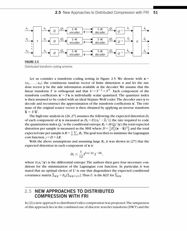
2.5 New Approaches to Distributed Compression with FRI 51
T...
Q
Q
Q
S-Wencoder Q21
Q21
Q21
U ...
Q1x1
x2
xn
x1
x2
xn
x1
x2
xnˆ
x1
x2
xnˆy
S-Wencoder
S-Wencoder
y
yS-W
decoder
S-Wdecoder
S-Wdecoder
'
Q2'
Qn'
Q1'
Q2'
Qn'
FIGURE 2.5
Distributed transform coding scheme.
Let us consider a transform coding setting in Figure 2.5. We denote with x�(x1, . . . , xn) the continuous random vector of finite dimension n and let the ran-dom vector y be the side information available at the decoder. We assume that thelinear transform T is orthogonal and that U �T �1 �T T . Each component of thetransform coefficients x��T x is individually scalar quantized. The quantizer indexis then assumed to be coded with an ideal Slepian–Wolf coder. The decoder uses y todecode and reconstruct the approximation of the transform coefficients x�. The esti-mate of the original source vector is then obtained by applying an inverse transformx � U x�.
The high-rate analysis in [26,27] assumes the following: the expected distortion Di
of each component of x is measured as Di �E[(xi�� xi�)]; the rate required to codethe quantization index Qi� is the conditional entropy Ri �H(Qi�|y); the total expecteddistortion per sample is measured as the MSE where D � 1
nE[‖x� x‖2]; and the total
expected rate per sample is R� 1n
∑i Ri .The goal was then to minimize the Lagrangian
cost function j�D ��R.With the above assumptions and assuming large Ri , it was shown in [27] that the
expected distortion in each component of x is
Di � 1
122h(xi�|y)2�2Ri ,
where h(xi�|y) is the differential entropy. The authors then gave four necessary con-ditions for the minimization of the Lagrangian cost function. In particular, it wasstated that an optimal choice of U is one that diagonalizes the expected conditionalcovariance matrix x|y �Ey[x|y(( y))]. Thus U is the KLT for x|y .
2.5 NEW APPROACHES TO DISTRIBUTEDCOMPRESSION WITH FRI
In [2] a new approach to distributed video compression was proposed.The uniquenessof this approach lies in the combined use of discrete wavelet transform (DWT) and the
52 CHAPTER 2 Distributed Transform Coding
concept of sampling of signals with finite rate of innovation (FRI),which shifts the taskof disparity compensation or motion estimation to the decoder side. The proposedscheme does not employ any traditional channel coding technique.
In this section,we will discuss the basic concepts behind this approach and showthe analysis of the rate-distortion bound for a simple example. For simplicity we willonly consider a simplified case of a translating bi-level polygon. We refer to [2] forresults of more general schemes with realistic cases. We start by presenting the mainresults of sampling FRI signals before moving on to the actual coding scheme.
2.5.1 Background on Sampling of 2D FRI Signals
The definition and sampling schemes of FRI signals are given in detail in [5, 6, and33]. We will only discuss the main results that will be used in the sequel. Let a 2Dcontinuous signal be f (x, y) with x, y∈R and let the 2D sampling kernel be �(x, y).In a typical sampling setup, the samples obtained by sampling f (x, y) with �(x, y) aregiven by
Sm,n � 〈 f (x, y), �(x/T �m, y/T �n)〉,where 〈·〉 denotes the inner product and m, n∈Z. Assume that the sampling kernelsatisfies the polynomial reproduction property that is,∑
m∈Z
∑n∈Z
c(p,q)m,n �(x �m, y �n)�x pyq (2.18)
with p, q∈Z and a proper set of coefficients c(p,q)m,n . It follows that, with T �1, the
continuous geometric moment mp,q of order (p�q) of the signal f (x, y) is given by
mp,q �∑m∈Z
∑n∈Z
c( p,q)m,n Sm,n. (2.19)
Therefore, given a set of coefficients c( p,q)m,n , one can retrieve the continuous moments
from an arbitrarily low-resolution set of samples Sm,n provided that f (x, y) lies in theregion where Equation (2.19) is satisfied.
The polynomial reproduction property is satisfied by any valid scaling function�j(x, y) of theWT,where j represents the number of levels of the wavelet decomposi-tion. Thus we can change the resolution of Sm,n by altering j with the corresponding
sampling period of T �2 j . It can be shown that the required coefficients c(p,q)m,n are
given by
c(p,q)m,n �
⟨x pyq, �j(x �m, y �n)
⟩(2.20)
where �j(x, y) is the dual of �j(x, y). In the next section, we show that the motionparameters can be extracted from the set of continuous moments mp,q obtained usingEquation (2.19).
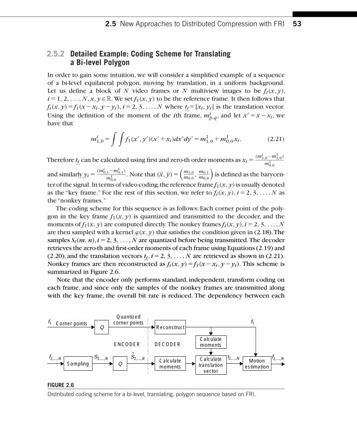
2.5 New Approaches to Distributed Compression with FRI 53
2.5.2 Detailed Example: Coding Scheme for Translatinga Bi-level Polygon
In order to gain some intuition, we will consider a simplified example of a sequenceof a bi-level equilateral polygon, moving by translation, in a uniform background.Let us define a block of N video frames or N multiview images to be fi(x, y),i �1, 2, . . . , N , x, y∈R. We set f1(x, y) to be the reference frame. It then follows thatfi(x, y)� f1(x �xi, y �yi), i �2, 3, . . . , N where ti� [xi, yi] is the translation vector.Using the definition of the moment of the ith frame, mi
p,q, and let x��x �xi , wehave that
mi1,0 �
∫ ∫f1(x�, y�)(x��xi)dx�dy��m1
1,0 �m10,0 xi. (2.21)
Therefore ti can be calculated using first and zero-th order moments as xi �(mi
1,0�m11,0)
m10,0
and similarly yi �(mi
0,1�m10,1)
m10,0
. Note that (x, y)�(
m1,0m0,0
,m0,1m0,0
)is defined as the barycen-
ter of the signal. In terms of video coding,the reference frame f1(x, y) is usually denotedas the “key frame.” For the rest of this section, we refer to fi(x, y), i �2, 3, . . . , N asthe “nonkey frames.”
The coding scheme for this sequence is as follows: Each corner point of the poly-gon in the key frame f1(x, y) is quantized and transmitted to the decoder, and themoments of f1(x, y) are computed directly.The nonkey frames fi(x, y), i �2, 3, . . . , Nare then sampled with a kernel �(x, y) that satisfies the condition given in (2.18).Thesamples Si(m, n), i �2, 3, . . . , N are quantized before being transmitted.The decoderretrieves the zero-th and first-order moments of each frame using Equations (2.19) and(2.20), and the translation vectors ti , i �2, 3, . . . , N are retrieved as shown in (2.21).Nonkey frames are then reconstructed as fi(x, y)� f1(x �xi, y �yi). This scheme issummarized in Figure 2.6.
Note that the encoder only performs standard, independent, transform coding oneach frame, and since only the samples of the nonkey frames are transmitted alongwith the key frame, the overall bit rate is reduced. The dependency between each
Q
Sampling Q
Reconstruct
Calculatemoments
Calculatetranslation
vector
Motionestimation
Quantizedcorner pointsCorner points
f2,...,N
f1 f1
S2,...,N S2,...,N t2,...,N f2,...,Nˆ
ENCODER DECODERCalculatemoments
FIGURE 2.6
Distributed coding scheme for a bi-level, translating, polygon sequence based on FRI.

54 CHAPTER 2 Distributed Transform Coding
frame is exploited at the decoder via joint decoding. Thus, this coding scheme has alow-complexity encoder.
In the following section, we will examine the distortion-rate behavior of this dis-tributed coding scheme and compare the rate-distortion performance with that of anideal joint (interframe) coder and an ideal independent (intraframe) coder.
2.5.2.1 Rate-distortion Analysis: Joint Encoder and Independent EncoderFigure 2.7 presents an example of a bi-level polygon in a uniform background and avisualization of the reconstruction error as a result of a mismatch between the valuesof a translation vector at the encoder and the decoder.
For the ideal joint encoder,we assume that the location of each corner point of thepolygon and the frame-by-frame translation vectors ti are quantized and transmittedto the decoder directly. The independent encoder on the other hand transmits thequantized corner points of every video frame to the decoder.
Let fi(x, y), i �1, 2, . . . , N be an N -frame video sequence with size A�A that con-tains a bi-level,equilateral polygon of C corner points with amplitude B. First we wantto find the theoretical distortion-rate bound of an ideal joint encoder. The distortionD is always measured as the mean-squared error (MSE) in the following analysis.
The joint encoder has to quantize two sets of parameters: the corner points andthe translation vectors. Thus we have two types of distortion that are independentand additive, which can then be analyzed separately. Furthermore, at high bit rate, wecan also assume that, for each parameter, the quantization errors along the x-directionand y-direction in the Cartesian coordinate are independent and,hence, also additive.Lastly, we assume that the locations of the corner points are independent.
Let RC be the number of bits allocated to represent each corner point and let RT
denote the number of bits allocated to represent each translation vector. With theabove assumption, one can show that the optimal bit allocation that minimizes D forthis joint encoder is given by
RC �RT �RE ,
Object
FIGURE 2.7
(Left) A bi-level square in a uniform background. (Right) A visualization of the reconstruction errorresulting from the mismatch between the values of a translation vector at the encoder and thedecoder.
2.5 New Approaches to Distributed Compression with FRI 55
where the constant RE �2 log2
(N
2(N�1)
). At a high rate, the distortion-rate bound
DINTER(R) is
DINTER(R)�2A2B2CINTER
(2� R
2(C�N�1)
),
where R is the total number of bits and CINTER is a constant.We also want to find the distortion-rate bound of the independent coder. In this
case the total number of bits used to encode the sequence is R�NCRC .With the sameset of assumptions as above, one can also show that, at a high rate, the distortion-rateDINTRA(R) bound of the independent coder is given by
DINTRA(R)�2A2B2(
2� R2(NC)
).
Note that the decay rate of DINTER(R),which equals 2� R2(C�N�1) , is greater than that
of DINTRA(R) given by 2� R2(NC) for C �1. This is as expected since the joint encoder
exploits the interframe dependency of the video sequence and achieves a better com-pression efficiency. In the next section, we will examine the distortion-rate behaviorof the proposed FRI-based distributed coding scheme.
2.5.2.2 Rate-distortion Analysis: Distributed Coding Using Samplingof FRI Signals
In the proposed scheme shown in Figure 2.6, there are still two sets of parametersto be quantized: the corner points and the samples. The quantization errors in thesamples lead to errors in the retrieved translation vectors.Thus,we have two types ofdistortion: the distortion due to the error in the retrieved translation vector as a resultof quantization of the transmitted samples and the distortion due to quantization ofcorner points.As with the previous analysis,we assume that the two types of distortionare independent.
Given the observed samples, Sm,n, of size Lm �Ln, from the sampling scheme ofFRI signals, clearly, the errors introduced by quantizing Sm,n lead to an error in theretrieved moment Mp,q. In the proposed coding scheme,the frame-to-frame translationvector can be obtained by calculating the barycenters of the two video frames. The
barycenter in the Cartesian coordinate is defined as(
M1,0M0,0
,M0,1M0,0
),where M1,0
M0,0and M0,1
M0,0
are in fact normalized first-order moments. Let us denote the normalized momentof order (p�q) as Mp,q �
Mp,q
M0,0and let Sm,n � Sm,n �em,n, where Sm,n denotes the
quantized samples and em,n represents the quantization error; we have that
Mp,q �
Lm∑m
Ln∑n
Cp,qm,n
M0,0Sm,n �
Lm∑m
Ln∑n
Cp,qm,n
M0,0em,n �Mp,q �wp,q,
where Cp,qm,n are the normalized polynomial reproduction coefficients.
Let us denote with Mip,q �M
i
p,q �wip,q, the normalized moment of the ith frame.
It is easy to show that the error in the frame-to-frame translation vector between the

56 CHAPTER 2 Distributed Transform Coding
ith and jth frame is then given by (qSx, qS
y) where qSx �(wi
1,0 �wj1,0) represents the
error in the x-component of the translation vector. Similarly, qSy �(wi
0,1 �wj0,1) is the
error in the y-component.Since each sample is independently scalar quantized, one can assume that the
probability density function (PDF) of wp,q is Gaussian whose variance depends on
the set of polynomial reproduction coefficients Cp,qm,n. We also assume that the errors
in each direction of the retrieved translation vector are independent, that is, qSx and
qSy are independent. With these assumptions, it is possible to show that the distortion
due to the quantization of the samples, as denoted by DS , is given by
DS �16AB2
√2�
(�0(C
1,0m,n)��0(C
0,1m,n)
)2�ns ,
where ns is the number of bits allocated to represent each sample and �0 is a constant.It can then be shown that the optimal bit allocation is
RC
2�nS �RS,
with the constant RS � log2
(A√
2�16
N(N�1)
(�0(C
1,0m,n)��0(C
0,1m,n)
)�1)
. Note that RC is
the number of bits allocated to represent each corner point. Finally, it follows thatthe theoretical distortion-rate bound, DDSC_FRI (R), of this proposed coding scheme isgiven by
DDSC_FRI (R)�2 A B2CDSC_FRI 2� R
2C�(N�1)LmLn
2 , (2.22)
where CDSC_FRI is a constant.Equation (2.22) shows us that the decay rate of DDSC_FRI (R) is equal to
2� R
2C�(N�1)LmLn
2 ,which is always lower than the rate of 2� R2(C�N�1) of the joint encoder.
However, in comparison with the independent encoder whose decay rate equals
2� R2(NC) , the decay rate of the distortion of the proposed FRI-based coding scheme
can be higher depending on the value of C and LmLn. The value of LmLn decreases asthe level of wavelet decomposition increases, which results in a better compressionperformance. Thus, we ideally want the level of wavelet decomposition to be as highas possible as there will be fewer coefficients to be transmitted.
Another point to be noted is that as the number of corner points C becomes larger,our proposed coding method performs relatively better than the independent encoder.The key point here is that as the complexity of the object in the video frame increases,this FRI-based distributed coding scheme can achieve better compression efficiencythan the independent encoder. This is because, with this scheme, we only need toencode the complex object once in the key frame. However, when C is small, weare better off by just transmitting the simple object in every video frame rather thantransmitting a number of samples.

2.5 New Approaches to Distributed Compression with FRI 57
102 103
10220
10240
100
R
D(R
)C 5 10
Joint encoderIndependent encoderDSC with sampling of FRI
103 104
R
C 5 100
D(R
)
10250
102100
100
104 105
D(R
)
10250
102100
100
R
C 5 1000
D(R
)
10250
102100
100
105 106
R
C 5 10000
FIGURE 2.8
Plots of DINTER(R) DINTRA(R) and DDSC_FRI(R). The complexity, C, of the sequence was set to 10,100, 1000, and 10,000. A Daubechies db2 filter was used and the parameters were: N�8,Lm �8, and Ln �8.
Figure 2.8 shows the plots of the distortion-rate bound for the three codingschemes. A Daubechies db2 filter was used with eight levels of wavelet decompo-sition. The size of the observed samples was set to 8�8. From the plots, at C �10,the independent (intraframe) coder achieves higher compression efficiency than theFRI-based distributed coding scheme. However, the proposed scheme outperformsthe independent coder as the number of corner points increases. The performancegap between the joint (interframe) encoder and the proposed scheme also decreasesas the complexity of the object in the sequence increases.
The plots shown in Figure 2.8 have been validated in [2] with synthesized videosequences of translating bi-level polygons with a different number of corner points.The scheme has also been extended to the case of a real object whose motion can bedescribed by an affine transform (see [2]). Even with a real object and a more complexmotion model, the same intuition remains: it makes sense to encode a complex objectonce and then transmit only the samples (i.e., the low-pass coefficients of the WT) ofthe object for the rest of the sequence.

58 CHAPTER 2 Distributed Transform Coding
2.6 CONCLUSIONSIn this chapter, we started by reviewing the main known results on transform codingin the centralized compression scenario, we then looked at the distributed transformcoding problem that arises when the source is not available at a single location but isdistributed at multiple sites. Extensions of the KLT to the distributed case were firstpresented, and then possible variations of DCT and WT were discussed.
Although there are scenarios where precise answers to the correct design of a dis-tributed transform coder can be provided,in most situations the solutions are based onheuristics and optimal distributed transforms are not known yet.This clearly indicatesthat the distributed transform coding problem is still widely open and that a vast spaceof unexplored solutions remain to be discovered.
REFERENCES[1] E. Setton, A.Aaron,S. Rane,and B. Girod.Transform-domainWyner–Ziv codec for video. In Proc.
Visual Communications and Image Processing, VCIP-2004, San Jose, CA, January 2004.
[2] V. Chaisinthop and P. L. Dragotti.A new approach to distributed coding using sampling of signalswith finite rate of innovation. In Proc. Picture Coding Symposium 2007, Lisbon, Portugal,November 2007.
[3] N.-M. Cheung, C. Tang, A. Ortega, and C. S. Raghavendra. Efficient wavelet-basedpredictive Slepian–Wolf coding for hyperspectral imagery. Signal Process., 86(11):3180–3195, 2006.
[4] A. Cohen, I. Daubechies, O. Guleryuz, and M. T. Orchard. On the importance of combiningwavelet-based non-linear approximation with coding strategies. IEEE Trans. on InformationTheory, 48(7):1895–1921, July 2002.
[5] P. L. Dragotti, M. Vetterli, and T. Blu. Exact sampling results for signals with finite rate of inno-vation using Strang–Fix conditions and local kernels. In Proc. of IEEE Int. Conf. on Acoustic,Speech and Signal Processing (ICASSP), Philadelphia, PA, March 2005.
[6] P. L. Dragotti,M. Vetterli, andT. Blu. Sampling moments and reconstructing signals of finite rateof innovation: Shannon meets Strang–Fix. IEEE Trans.on Signal Processing, 55(5):1741–1757,May 2007.
[7] N. Farvardin and J. Modestino. Optimum quantizer performance for a class of non-Gaussianmemoryless sources. Information Theory, IEEE Transactions on, 30(3):485–497, May 1984.
[8] M. Flierl and P. Vandergheynst. Distributed coding of highly correlated image sequences withmotion-compensated temporal wavelets. Eurasip Journal Applied Signal Processing, 2006,September 2006.
[9] M. Gastpar, P. L. Dragotti, and M. Vetterli. The distributed Karhunen–Loève transform. InMultimedia and Signal Processing Workshop,Virgin Islands, December 2002.
[10] M. Gastpar, P. L. Dragotti, and M. Vetterli. The distributed, partial and conditional Karhunen–Loève transforms. In Data Compression Conference, Snowbird, Utah, March 2003.
[11] M. Gastpar, P. L. Dragotti, and M. Vetterli. On compression using the distributed Karhunen–Loève transform. In Proc.of IEEE Int.Conf.on Acoustic, Speech and Signal Processing, invitedpaper, Montreal (CA), May 2004.

References 59
[12] M. Gastpar, P. L. Dragotti, and M. Vetterli. The distributed Karhunen–Loève transform. IEEETrans. on Information Theory, 52 (12):5177–5196, December 2006.
[13] A. Gersho and R. M. Gray. Vector Quantization and Signal Compression. Kluwer AcademicPublishers, Norwell, MA, 1991.
[14] B. Girod, A. M.Aaron,S. Rane,and D. Rebollo-Monedero. Distributed video coding. Proceedingsof the IEEE, 93(1):71–83, 2005.
[15] V. K Goyal. Theoretical foundations of transform coding. IEEE Signal Processing Magazine,18(5):9–21, September 2001.
[16] R. M. Gray and D. L. Neuhoff. Quantization. Information Theory, IEEE Transactions on,44(6):2325–2383, October 1998.
[17] C. Guillemot and A. Roumy. Towards constructive Slepian–Wolf coding schemes. In DistributedSource Coding: Theory, Algorithms and Applications, eds. P. L. Dragotti and M. Gastpar,Academic Press, Elsevier, San Diego, CA, 2009.
[18] J. Huang and P. Schultheiss. Block quantization of correlated Gaussian random variables.Communications, IEEE Transactions on [legacy, pre-1988], 11(3):289–296, September 1963.
[19] D. A. Huffman. A method for the construction of minimum-redundancy codes. Proceedings ofthe IRE, 40(9):1098–1101, 1952.
[20] D. T. Lee. JPEG2000: Retrospective and new developments. Proceedings of the IEEE, 93(1):32–41, 2005.
[21] S. Mallat. A Wavelet Tour of Signal Processing. Academic Press, Boston, MA, 1998.
[22] H. Nurdin,R. R. Mazumdar,andA. Bagchi. On estimation and compression of distributed corre-lated signals with incomplete observations. In Proc. Conf. Mathematical Theory of Networksand Systems, Leuven (Belgium), July 2004.
[23] A. Ortega and K. Ramchandran. Rate-distortion methods for image and video compression.Signal Processing Magazine, IEEE, 15(6):23–50, 1998.
[24] F. Pereira, C. Brites, and J. Ascenso. Distributed video coding: Basics, codecs and performance.In Distributed Source Coding: Theory, Algorithms and Applications, eds. P. L. Dragotti andM. Gastpar, Academic Press, Elsevier, San Diego, CA, 2009.
[25] R. Puri and K. Ramchandran. PRISM: A video coding architecture based on distributed compres-sion principles. In 40th Allerton Conference on Communication, Control and Computing,Allerton, IL, October 2002.
[26] D. Rebollo-Monedero and B. Girod. Quantization for distributed source coding. In DistributedSource Coding: Theory, Algorithms and Applications, eds. P. L. Dragotti and M. Gastpar,Academic Press, Elsevier, San Diego, CA, 2009.
[27] D. Rebollo-Monedero, S. Rane, A. Aaron, and B. Girod. High-rate quantization and transformcoding with side information at the decoder. Eurasip Signal Processing Journal, 86(11):3160–3179, November 2006. Special Issue on Distributed Source Coding.
[28] O. Roy and M. Vetterli. On the asymptotic distortion behavior of the distributed Karhunen–Loève transform. In Proc. of Allerton Conf. Communication, Control and Computing,Monticello (IL), September 2005.
[29] O. Roy and M. Vetterli. Dimensionality reduction for distributed estimation in the infinitedimensional regime. IEEE Trans. on Information Theory, 54(4):1655–1669, April 2008.
[30] D. Slepian and J. Wolf. Noiseless coding of correlated information sources. IEEE Transactionson Information Theory, 19(4):471–480, 1973.
[31] G. J. Sullivan and T. Wiegand. Video compression—from concepts to the H.264/AVC standard.Proceedings of the IEEE, 93(1):18–31, 2005.
[32] M. Vetterli. Wavelets, approximation and compression. IEEE Signal Processing Magazine,18:59–73, September 2001.
60 CHAPTER 2 Distributed Transform Coding
[33] M. Vetterli, P. Marziliano, and T. Blu. Sampling signals with finite rate of innovation. IEEETransactions on Signal Processing, 50(6):1417–1428, 2002.
[34] G. K.Wallace.The JPEG still picture compression standard. Commun. ACM,34(4):30–44,1991.
[35] I. H. Witten, R. M. Neal, and J. G Cleary. Arithmetic coding for data compression. Commun.ACM, 30(6):520–540, 1987.
[36] A. Wyner and J. Ziv. The rate-distortion function for source coding with side information at thedecoder. IEEE Transactions on Information Theory, 22(1):1–10, 1976.
[37] K. S. Zhang,X. R. Li,P. Zhang, and H. F. Li. Optimal linear estimation fusion part IV: Sensor datacompression. In Proc. of Int. Conf. Fusion, Queensland (Australia), July 2003.
CHAPTER
3Quantization for DistributedSource Coding
David Rebollo-MonederoDepartment of Telematics Engineering,
Universitat Politècnica de Catalunya,
Barcelona, Spain
Bernd GirodDepartment of Electrical Engineering,
Stanford University, Palo Alto, CA
C H A P T E R C O N T E N T SIntroduction . . . . . . . . . . . . . . . . . . . . . . . . . . . . . . . . . . . . . . . . . . . . . . . . . . . . . . . . . . . . . . . . . . . . . . . . . . . . . . 62Formulation of the Problem .. . . . . . . . . . . . . . . . . . . . . . . . . . . . . . . . . . . . . . . . . . . . . . . . . . . . . . . . . . . . . 64
Conventions . . . . . . . . . . . . . . . . . . . . . . . . . . . . . . . . . . . . . . . . . . . . . . . . . . . . . . . . . . . . . . . . . . . . . . . . 64Network Distributed Source Coding . . . . . . . . . . . . . . . . . . . . . . . . . . . . . . . . . . . . . . . . . . . . . . . . 65Cost, Distortion, and Rate Measures . . . . . . . . . . . . . . . . . . . . . . . . . . . . . . . . . . . . . . . . . . . . . . . 66Optimal Quantizers and Reconstruction Functions . . . . . . . . . . . . . . . . . . . . . . . . . . . . . . . . 67Example: Quantization of Side Information . . . . . . . . . . . . . . . . . . . . . . . . . . . . . . . . . . . . . . . . 67
Optimal Quantizer Design . . . . . . . . . . . . . . . . . . . . . . . . . . . . . . . . . . . . . . . . . . . . . . . . . . . . . . . . . . . . . . . . 68Optimality Conditions . . . . . . . . . . . . . . . . . . . . . . . . . . . . . . . . . . . . . . . . . . . . . . . . . . . . . . . . . . . . . . 68Lloyd Algorithm for Distributed Quantization . . . . . . . . . . . . . . . . . . . . . . . . . . . . . . . . . . . . . . 69
Experimental Results . . . . . . . . . . . . . . . . . . . . . . . . . . . . . . . . . . . . . . . . . . . . . . . . . . . . . . . . . . . . . . . . . . . . 70High-rate Distributed Quantization . . . . . . . . . . . . . . . . . . . . . . . . . . . . . . . . . . . . . . . . . . . . . . . . . . . . . . 73
High-rate WZ Quantization of Clean Sources. . . . . . . . . . . . . . . . . . . . . . . . . . . . . . . . . . . . . . . 74High-rate WZ Quantization of Noisy Sources. . . . . . . . . . . . . . . . . . . . . . . . . . . . . . . . . . . . . . . 76High-rate Network Distributed Quantization . . . . . . . . . . . . . . . . . . . . . . . . . . . . . . . . . . . . . . . 80
Experimental Results Revisited . . . . . . . . . . . . . . . . . . . . . . . . . . . . . . . . . . . . . . . . . . . . . . . . . . . . . . . . . . 84Conclusions . . . . . . . . . . . . . . . . . . . . . . . . . . . . . . . . . . . . . . . . . . . . . . . . . . . . . . . . . . . . . . . . . . . . . . . . . . . . . . 85References . . . . . . . . . . . . . . . . . . . . . . . . . . . . . . . . . . . . . . . . . . . . . . . . . . . . . . . . . . . . . . . . . . . . . . . . . . . . . . . 86
Distributed Source Coding: Theory, Algorithms, and ApplicationsCopyright © 2008 by Academic Press, Inc. All rights of reproduction in any form reserved. 61

62 CHAPTER 3 Quantization for Distributed Source Coding
3.1 INTRODUCTIONConsider the sensor network depicted in Figure 3.1, where sensors obtain noisyreadings of some unseen data of interest that must be transmitted to a central unit.The central unit has access to side information, for instance, archived data or readingsfrom local sensors. At each sensor,neither the noisy observations of the other sensorsnor the side information is available. Nevertheless, the statistical dependence amongthe unseen data, the noisy readings, and the side information may be exploited in thedesign of each individual sensor encoder and the joint decoder at the central unit tooptimize the rate-distortion performance. Clearly, if all the noisy readings and the sideinformation were available at a single location, traditional joint denoising and encod-ing techniques could be used to reduce the transmission rate as much as possible,for a given distortion. However, since each of the noisy readings must be individuallyencoded without access to the side information,practical design methods for efficientdistributed coders of noisy sources are needed.
The first attempts to design quantizers for Wyner–Ziv (WZ) coding—that is, lossysource coding of a single instance of directly observed data with side information at thedecoder—were inspired by the information-theoretic proofs. Zamir and Shamai [50,51] proved that under certain circumstances,linear codes and high-dimensional nestedlattices approach the WZ rate-distortion function, in particular if the source data andside information are jointly Gaussian. This idea was further developed and appliedby Pradhan et al. [21, 29, 30] and Servetto [38], who published heuristic designs and
Remote Sensor
Remote Sensor
Remote Sensor
Local Sensor
SideInformation
Central Unit
FIGURE 3.1
Distributed source coding in a sensor network.

3.1 Introduction 63
performance analysis focusing on the Gaussian case, based on nested lattices, witheither fixed-rate coding or entropy coding of the quantization indices.
A different approach was followed by Fleming and Effros [11], who generalizedthe Lloyd algorithm [26] for locally optimal, fixed-rate WZ quantization design. Later,Fleming, Zhao, and Effros [12] included rate-distortion optimized quantizers in whichthe rate measure is a function of the quantization index, for example, a codewordlength. Unfortunately, vector quantizer dimensionality and entropy code blocklengthare identical in their formulation; thus the resulting quantizers either lack inperformance or are prohibitively complex. An efficient algorithm for finding glob-ally optimal quantizers among those with contiguous code cells was provided in [27],although, regrettably, it has been shown that code cell contiguity precludes optimal-ity in general distributed settings [9]. Cardinal and Van Asche [5] considered Lloydquantization for ideal symmetric Slepian–Wolf (SW) coding without side information.Cardinal [3, 4] has also studied the problem of quantization of the side informationitself for lossless distributed coding of discrete source data (which is not quantized).
It may be concluded from the proof of the converse to the WZ rate-distortion the-orem [42] that there is no asymptotic loss in performance by considering block codesof sufficiently large length,which may be seen as vector quantizers, followed by fixed-length coders.This suggests a convenient implementation ofWZ coders as quantizers,possibly preceded by transforms, followed by SW coders, analogous to the implemen-tation of nondistributed coders.This implementation is represented in Figure 3.2.Thequantizer divides the signal space into cells, which, however, may consist of non-contiguous subcells mapped into the same quantizer index. Xiong et al. [25, 43]implemented a WZ coder as a nested lattice quantizer followed by a SW coder, andin [45], a trellis-coded quantizer was used instead (see also [44]).
An extension of the Lloyd algorithm, more general than Fleming and Effros’s,appeared in our own work [37], which considered a variety of coding settings in aunified framework,including the important case of ideal SW distributed coding of oneor several sources with side information, that is,when the rate is the joint conditionalentropy of the quantization indices given the side information.
An upper bound on the rate loss due to the unavailability of the side informationat the encoder was found by Zamir [47], who also proved that for power-differencedistortion measures and smooth source probability distributions,this rate loss vanishes
Slepian–Wolf
Encoder
Slepian–Wolf
Decoder
Y
X Q Q XMinimum-Distortion
ReconstructionQuantizer
Y
Wyner–Ziv Encoder Wyner–Ziv Decoder
ˆ
FIGURE 3.2
A practical WZ coder obtained by cascading a quantizer and a SW coder.

64 CHAPTER 3 Quantization for Distributed Source Coding
in the limit of small distortion. A similar high-resolution result was obtained by Zamirand Berger [48] for distributed coding of several sources without side information,also from an information-theoretic perspective, that is, for arbitrarily large dimension.In [40] (unpublished),it was shown that tessellating quantizers followed by SW codersare asymptotically optimal in the limit of small distortion and large dimension.The firsttheoretic characterization of high-rate WZ quantizers with SW coding was presentedin our own work [32]. It was inspired by the traditional developments of high-ratequantization theory, specifically Bennett’s distortion approximation [1, 28], Gish andPierce’s rate approximation [17], and Gersho’s conjecture [15].
As for quantization of a noisy observation of an unseen source, the nondistributedcase was studied by Dobrushin,Tsybakov,Wolf, Ziv, Ephraim, Gray, and others [8, 10,41]. Most of the operational work on distributed coding of noisy sources, that is, fora fixed dimension, deals with quantizer design for a variety of settings, as in the workby Lam and Reibman [22,23],and Gubner [20],but does not consider entropy codingor the characterization of such quantizers at high rates or transforms. The problemof optimal noisy WZ quantizer design with side information at the decoder and idealSW coding has only been studied under the assumptions of high rates and particularstatistical conditions by our research group [36].
This chapter investigates the design of rate-distortion optimal quantizers for dis-tributed compression in a network with multiple senders and receivers. In such anetwork, several noisy observations of one or more unseen sources are separatelyencoded by each sender and the quantization indices transmitted to a number ofreceivers, which jointly decode all available transmissions with the help of side infor-mation locally available. We present a unified framework in which a variety of codingsettings is allowed, including ideal SW coding, along with an extension of the Lloydalgorithm for “locally”optimal design. In addition,we characterize optimal quantizersin the limit of high rates and approximate their performance. This work summarizespart of the research detailed in [31] and a number of papers, mainly [34, 35], whereadditional mathematical technicalities and proofs can be found.
Section 3.2 contains the formulation of the problem studied.A theoretic analysis foroptimal quantizer design is presented in Section 3.3. In Section 3.5,optimal quantizersand their performance are characterized asymptotically at high rates. Experimentalresults for distributed coding of jointly Gaussian data are shown in Section 3.4 andrevisited in Section 3.6.
3.2 FORMULATION OF THE PROBLEM3.2.1 Conventions
Throughout the chapter, the measurable space in which a random variable (r.v.) takeson values will be called an alphabet. All alphabets are assumed to be Polish spaces toensure the existence of regular conditional probabilities. We shall follow the conven-tion of using upper-case letters for r.v.’s,and lower-case letters for particular values they
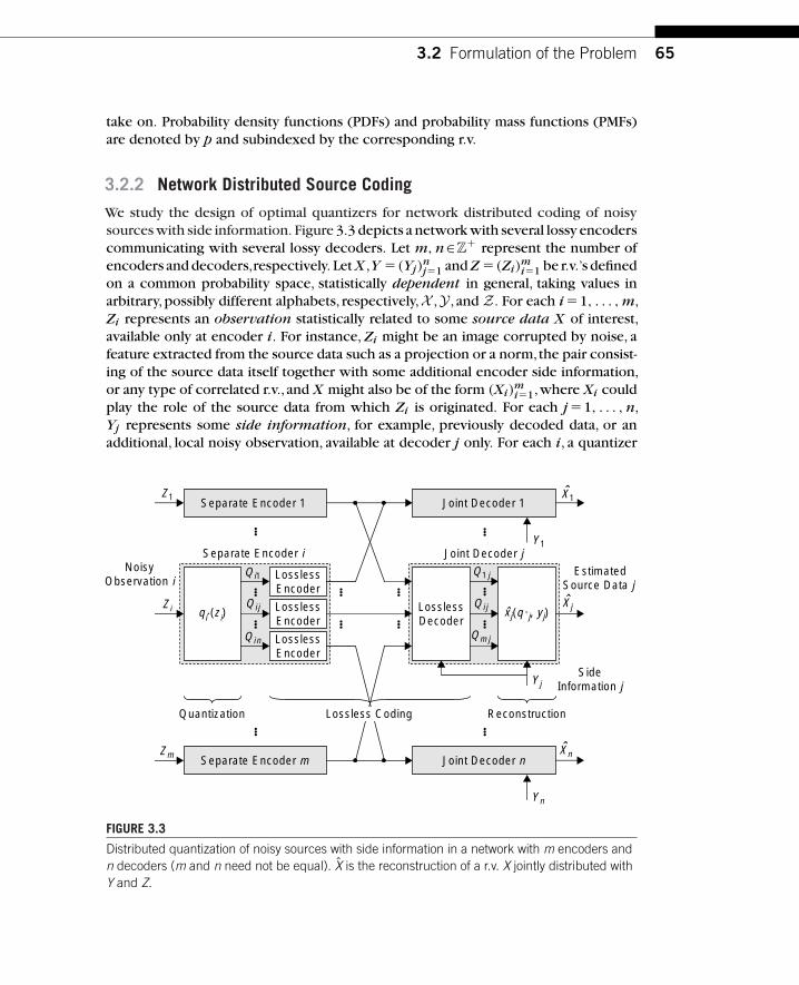
3.2 Formulation of the Problem 65
take on. Probability density functions (PDFs) and probability mass functions (PMFs)are denoted by p and subindexed by the corresponding r.v.
3.2.2 Network Distributed Source Coding
We study the design of optimal quantizers for network distributed coding of noisysources with side information. Figure 3.3 depicts a network with several lossy encoderscommunicating with several lossy decoders. Let m, n∈Z
� represent the number ofencoders and decoders,respectively. Let X ,Y �(Yj)
nj�1 and Z �(Zi)
mi�1 be r.v.’s defined
on a common probability space, statistically dependent in general, taking values inarbitrary,possibly different alphabets, respectively,X ,Y , and Z. For each i �1, . . . , m,Zi represents an observation statistically related to some source data X of interest,available only at encoder i. For instance, Zi might be an image corrupted by noise, afeature extracted from the source data such as a projection or a norm,the pair consist-ing of the source data itself together with some additional encoder side information,or any type of correlated r.v., and X might also be of the form (Xi)
mi�1,where Xi could
play the role of the source data from which Zi is originated. For each j �1, . . . , n,Yj represents some side information, for example, previously decoded data, or anadditional, local noisy observation, available at decoder j only. For each i, a quantizer
NoisyObservation i
EstimatedSource Data j
SideInformation j
Joint Decoder j Separate Encoder i
Z1
Y1
ReconstructionQuantization Lossless Coding
LosslessEncoder
LosslessEncoder
LosslessEncoder
LosslessDecoder
Joint Decoder 1Separate Encoder 1
Separate Encoder m Joint Decoder n
Q1j
Qij
Qmj
(q ·j, yj)
Yj
Zm
qi·(zi)
Yn
Qi1
Zi Qij
Qin
X1ˆ
Xjˆ
Xnˆ
xj ˆ
FIGURE 3.3
Distributed quantization of noisy sources with side information in a network with m encoders andn decoders (m and n need not be equal). X is the reconstruction of a r.v. X jointly distributed withY and Z.

66 CHAPTER 3 Quantization for Distributed Source Coding
qi·(zi)�(qij(zi))nj�1, which can also be regarded as a family of quantizers, is applied
to the observation Zi ,obtaining the quantization indices Qi·�(Qij)nj�1. Each quantiza-
tion index Qij is losslessly encoded at encoder i and transmitted to decoder j, whereit is losslessly decoded. We shall see that both encoding and decoding of quantiza-tion indices may be joint or separate. For each j, all quantization indices receivedby decoder j, Q·j �(Qij)
mi�1, and the side information Yj are used jointly to estimate
the unseen source data X . Let Xj represent this estimate, obtained with a measurable
function xj(q·j, yj), called reconstruction function, in an alphabet Xj possibly differ-ent from X . Define Q�(Qij)
m,ni�1,j�1, X �(Xj)
nj�1, and x(q, y)�(xj(q·j, yj))
nj�1. Q and
X will denote the alphabets of Q and X , respectively. Partially connected networksin which encoder i does not communicate with decoder j can easily be handled byredefining Qi·, Q·j and Q not to include Qij .
3.2.3 Cost, Distortion, and Rate Measures
We shall now extend the concept of rate measure presented in [37] by means of amuch more general definition,accompanied by a characteristic property that will playa major role in the extension of the Lloyd algorithm for optimized quantizer design,called update property. Even though the definition of rate measure and its updateproperty may seem rather abstract and complex initially,we shall see that it possessesgreat generality and is applicable to a wide range of problems.The terms cost measure,rate measure, and distortion measure, formally equivalent by definition,will be usedto emphasize different connotations in the context of applications,usually a Lagrangiancost,a transmission rate,and the distortion introduced by lossy decoding,respectively.
A cost measure is a nonnegative measurable function of the form c(q, x, x, y, z),possibly defined in terms of the joint probability distribution of (Q, X, Y , Z).1 Its asso-ciated expected cost is defined as C �E c(Q, X, X, Y , Z). Furthermore,a cost measurewill be required to satisfy the following update property. For any modification of thejoint probability distribution of (Q, X, Y , Z) preserving the marginal distribution of(X, Y , Z), there must exist an induced cost measure c�, consistent with the originaldefinition almost surely (a.s.) but expressed in terms of the modified distribution,satis-fying E c�(Q, X, Y , Z)� C,where the expectation is taken with respect to the originaldistribution.
An important example of rate measure is that corresponding to asymmetric SWcoding of a quantization index Q given side information Y .The achievable rate in thiscase has been shown to be H(Q|Y ), when the two alphabets of the random variablesinvolved are finite [39], in the sense that any rate greater than H(Q|Y ) would allowarbitrarily low probability of decoding error,but any rate less than H(Q|Y ) would not.
1 Rigorously, a cost measure may take as arguments probability distributions (measures) and proba-bility functions; that is, it is a function of a function.We shall become immediately less formal and callthe evaluation of the cost measure for a particular probability distribution or function, cost measureas well.

3.2 Formulation of the Problem 67
In [6], the validity of this result was generalized to countable alphabets, but it wasstill assumed that H(Y )��. We show in [31, App. A] (also [35]) that the asymmetricSW result remains true under the assumptions in this chapter, namely, for any Q in acountable alphabet and any Y in an arbitrary alphabet,possibly continuous,regardlessof the finiteness of H(Y ).
Concordantly, we define the rate measure r(q, y)�� log pQ|Y (q| y) to model theuse of an ideal SW coder, in the sense that both the decoding error probability andthe rate redundancy are negligible. Note that the very same rate measure would alsomodel a conditional coder with access to the side information at the encoder. Wecheck that the SW rate measure defined satisfies the update property. The rate mea-sure corresponding to any other PMF p�Q|Y would be r�(q, y)�� log p�Q|Y (q, y). Themodified associated rate would then be R��E r�(Q, Y ), where r� is defined in termsof the new PMF but the expectation is taken with respect to the original one. Clearly,R��R�D(pQ|Y ‖p�Q|Y )�0. It can be seen that all rate measures defined in [37] satisfythe update property, thereby making the corresponding coding settings applicable tothis framework.
If the alphabets of X , Y , Z , and X are equal to some common normed vectorspace, then an example of a distortion measure is d(x, x, y, z)��‖x � x‖2 ��‖y �x‖2 ��‖z � x‖2, for any �, �, �∈[0, �). An example of a cost measure suitable for dis-tributed source coding,the main focus of this work,is c(q, x, x, y)�d(x, x)�� r(q, y),where � is a nonnegative real number determining the rate-distortion trade-off in theLagrangian cost C �D�� R.
3.2.4 Optimal Quantizers and Reconstruction Functions
Given a suitable cost measure c(q, x, x, y, z), we address the problem of findingquantizers qi·(zi) and reconstruction functions xj(q·j, yj) to minimize the associatedexpected cost C.The choice of the cost measure leads to a particular noisy distributedsource coding system, including a model for lossless coding.
3.2.5 Example: Quantization of Side Information
Even though the focus of this work is the application represented in Figure 3.3, thegenerality of this formulation allows many others. For example, consider the cod-ing problem represented in Figure 3.4, proposed in [3]. A r. v. Z is quantized. Thequantization index Q is coded at rate R1 �H(Q) and used as side information fora SW coder of a discrete random vector X . Hence, the additional rate required isR2 �H(X |Q). We wish to find the quantizer q(z) minimizing C �R2 �� R1. It can beshown that r1(q)�� log pQ(q) and r2(x, q)�� log pX |Q(x| q) are well-defined ratemeasures, using an argument similar to that for � log pQ|Y (q| y). Therefore, this prob-lem is a particular case of our formulation. In fact, this is a noisy WZ, or a statisticalinference problem in which R2 plays the role of distortion, since minimizing H(X |Q)
is equivalent to minimizing I(Z;X)� I(Q;X), nonnegative by the data processinginequality, zero if and only if Q is a sufficient statistic.

68 CHAPTER 3 Quantization for Distributed Source Coding
q (z) EntropyDecoder
EntropyEncoder
Z
Slepian–WolfDecoder
X X
Separate Lossless Encoder Joint Lossless Decoder
Lossy Side Information Encoder
R1
R2
Slepian–WolfEncoder
FIGURE 3.4
Quantization of side information.
Aside from particularizations and variations of distributed coding problems suchas quantization of side information,quantization with side information at the encoder,broadcast with side information and an extension of the Blahut–Arimoto algorithmto noisy WZ coding, we find that our theoretical framework also unifies apparentlyunrelated problems such as the bottleneck method and Gauss mixture modeling. Anextensive list of examples appears in [31].
3.3 OPTIMAL QUANTIZER DESIGNIn this section we establish necessary conditions for the optimal quantization andreconstruction functions, analogous to the nearest neighbor and centroid conditionfound in conventional,nondistributed quantization. Each necessary condition may beinterpreted as the solution to a Bayesian decision problem. They will be expressedin terms of conditional cost measures, defined below, which play the role of con-ditional risks in Bayesian decision theory. These conditions will be used later todevelop an extension of the Lloyd algorithm suitable for distributed quantization. Adetailed, rigorous analysis of these conditions and the derived algorithm is presentedin [31].
3.3.1 Optimality Conditions
The conditional cost measure for encoder i is defined as
ci(qi·, zi)�E[[
c(Q, X, x(Q, Y ), Y , Z)]Qi·�qi· |zi
],
where [expression]substitution denotes substitution in an expression, that is, the expres-sion of the definition is evaluated at qi· and conditioned on the event {Zi �zi}. Observethat the conditional cost measure is completely determined by the joint distribution

3.3 Optimal Quantizer Design 69
of X , Y , and Z , the cost measure c(q, x, x, y, z), the quantization at other encoderspQ
i�·|Zi�(qi�·, zi�), and all the reconstruction functions, grouped as x(q, y). Using the
fact that Qi �qi(Zi) and iterated expectation, it is easy to see that for each sender i,E ci(Qi·, Zi)�C. In terms of Bayesian decision theory, the expectation of conditionalrisks gives the overall Bayes risk. This key property leads to the necessary optimalitycondition for the quantizer at sender i, which may be informally expressed as:
q∗i·(Zi)a.s.� arg min
qi·ci(qi·, Zi), (3.1)
provided that a minimum exists.Similarly to the sender cost measures, the conditional cost measure for
decoder j is
˜cj(q·j, xj, yj)�E[[c(Q, X, X, Y , Z)]Xj�xj|q·j, yj].
Observe that the defining expression is evaluated at xj and conditioned on the jointevent {Q·j �q·j, Yj �yj}, and it is completely determined by the joint distributionof X ,Y , and Z , the cost measure c(q, x, x, y, z), all quantizers, and the reconstructionfunctions at other decoders xj�(q·j�, yj�). As in the case of the sender cost measures,
it can be shown that for each j, E ˜cj(Q·j, Xj, Yj)�C. From this key property it followsthat an optimal reconstruction function must satisfy
x∗j (Q·j, Yj)a.s.� arg min
xj
˜cj(Q·j, xj, Yj), (3.2)
provided that a minimum exists, for each pair (q·j, yj) satisfying pQ·j |Yj (q·j |yj)�0(x∗j (q·j, yj) can be arbitrarily defined elsewhere).
3.3.2 Lloyd Algorithm for Distributed Quantization
The necessary optimality conditions (3.1) and (3.2), together with the rate updateproperty defining rate measures, suggest an alternating optimization algorithm thatextends the Lloyd algorithm to the quantizer design problem considered in this work:
1. Initialization: For each i �1, . . . , m, j �1, . . . , n, choose initial quantizers(q(1)
i· (zi))i , and initial reconstruction functions (x(1)j (q·j, yj))j . Set k�1 and
C(0) ��.
2. Cost measure update: Update the cost measure c(k)(q, x, x, y, z), completelydetermined by probability distributions involving Q(k), X , X , Y , and Z .
3. Convergence check: Compute the expected cost C(k) associated with thecurrent quantizers (q(k)
i· (zi))i , reconstruction functions x(k)j (q·j, yj), and cost
measure c(k)(q, x, x, y, z). Depending on its value with respect to C(k�1),continue or stop.

70 CHAPTER 3 Quantization for Distributed Source Coding
4. Quantization update:For each i,obtain the next optimal quantizer (q(k�1)i· (zi))i ,
in terms of the most current quantizers with index i� �� i, all reconstructionfunctions x(k)
j (q·j, yj), and the cost measure c(k)(q, x, x, y, z).
5. Reconstruction update: For each j, obtain the next optimal reconstructionfunction x(k�1)
j (q·j, yj), given the most current version of the reconstruction
functions with index j� �� j, all quantizers (q(k�1)i· (zi))i , and the cost measure
c(k)(q, x, x, y, z).
6. Increment k and go back to 2.
It can be proved that the sequence of costs C(k) in the above algorithm is nonin-creasing, and since it is nonnegative, it converges. In addition,any quantizer satisfyingthe optimality conditions (3.1) and (3.2), without ambiguity in any of the minimiza-tions involved, is a fixed point of the algorithm. Even though these properties do notimply per se that the cost converges to a local or global minimum, the experimentalresults in the next section show good convergence properties, especially when thealgorithm is combined with genetic search for initialization. Many variations on thealgorithm are possible, such as constraining the reconstruction function, for instance,imposing linearity in Y for each Q when the distortion is the mean-squared error ofthe estimate X , or any of the variations mentioned in [31, 37].
3.4 EXPERIMENTAL RESULTSIn the following section we report experimental results obtained by applying theextension of the Lloyd algorithm for distributed coding described in Section 3.3.2 totheWZ coding problem.We consider a simple,intuitive case,represented in Figure 3.5.Let X∼N (0, 1) and NY ∼N (0, 1/�Y ) be independent, and let Y �X �NY . We wishto design scalarWZ quantizers minimizing the Lagrangian cost C �D�� R,where thedistortion is the mean-squared error (MSE) D�E ‖X � X‖2,and the rate is that requiredby an ideal SW codec,R�H(Q|Y ).The information-theoretic distortion-rate function
Source DataX∼N(0, 1)
SWEncoder
SWDecoder x (q, y)
X
Y SideInformation
Ny∼N(0, 1/�Y)
q (x)Q Q ˆ
ˆ
FIGURE 3.5
Experimental setup for clean WZ quantization.

3.4 Experimental Results 71
for i.i.d. pairs drawn according to the statistics of X, Y is DWZX |Y (R)��2
X |Y 2�2R[42, §I.C](also [33,Theorem 2]).
For the case �Y �10 and several values of �, scalar WZ quantizers and reconstruc-tion functions were designed using the extension of the Lloyd algorithm developedin this work. A simple genetic search method was combined with the Lloyd algo-rithm to select initial quantizers based on their cost after convergence.The algorithmwas applied to a fine discretization of the joint PDF of X, Y , as a PMF with approxi-mately 2.0 ·105 points (x, y) contained in a two-dimensional ellipsoid of probability1�10�4 (according to the reference PDF), producing 919 different values for X and919 different values for Y .
The corresponding distortion-rate points are shown in Figure 3.6, along with theinformation-theoretic distortion-rate function and the distortion bound D0 ��2
X |Y .Recall that in nondistributed quantization, at high rates, asymptotically optimal scalarquantizers introduce a distortion penalty of 10 log10
�e6 �1.53 dB with respect to the
information-theoretic bound [16]. Note that the experimental results obtained for thisparticular WZ quantization setup exhibit the same behavior.
Two scalarWZ quantizers for R � 0.55 and R � 0.98 bit are depicted in Figure 3.7.Conventional high-rate quantization theory shows that uniform quantizers are asymp-totically optimal. Note that quantizer (b), corresponding to a higher rate thanquantizer (a),is uniform,and perhaps surprisingly,no quantization index is reused.Thisexperimental observation, together with the 1.53 dB distortion gap mentioned earlier,
0 0.2 0.4 0.6 0.8 1 1.20
0.02
0.04
0.06
0.08
0.1
0.12
0.14
D0�0.0909
Clean WZQuantizers
1D
R [bit]
D
WZ RDFunction
210 log10 D
0 0.2 0.4 0.6 0.8 1 1.2
�1.53 dB
8
10
12
14
16
18
20
R [bit]
WZ RDFunction
�10.414 dB
FIGURE 3.6
Distortion-rate performance of optimized scalar WZ quantizers with SW coding. R� 1k H(Q |Y ),
X∼N (0,1), NY∼N (0,1/10) independent, Y � X�NY.
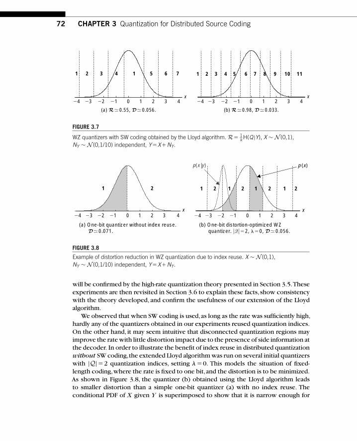
72 CHAPTER 3 Quantization for Distributed Source Coding
0
1 2 3 4 1 5 6 7
�4 �1�2�3 �4 �1�2�32 4x x
1 2 3 4 5 6 7 8 9 10 11
(b) R�0.98, D�0.033.(a) R�0.55, D�0.056.
1 3 0 2 41 3
FIGURE 3.7
WZ quantizers with SW coding obtained by the Lloyd algorithm. R� 1k H(Q |Y), X ∼ N (0,1),
NY ∼ N (0,1/10) independent, Y�X�NY.
1 2
x
1 2 1 2 1 2 1 2
p (x)p(x|y)
x2 424 21
(a) One-bit quantizer without index reuse.D�0.071.
(b) One-bit distortion-optimized WZ quantizer. u�u52, l50, D�0.056.
0 12223 24 2122230 2 41 3 3
FIGURE 3.8
Example of distortion reduction in WZ quantization due to index reuse. X ∼ N (0,1),NY ∼ N (0,1/10) independent, Y�X�NY.
will be confirmed by the high-rate quantization theory presented in Section 3.5.Theseexperiments are then revisited in Section 3.6 to explain these facts, show consistencywith the theory developed, and confirm the usefulness of our extension of the Lloydalgorithm.
We observed that when SW coding is used,as long as the rate was sufficiently high,hardly any of the quantizers obtained in our experiments reused quantization indices.On the other hand, it may seem intuitive that disconnected quantization regions mayimprove the rate with little distortion impact due to the presence of side information atthe decoder. In order to illustrate the benefit of index reuse in distributed quantizationwithout SW coding,the extended Lloyd algorithm was run on several initial quantizerswith |Q|�2 quantization indices, setting ��0. This models the situation of fixed-length coding,where the rate is fixed to one bit,and the distortion is to be minimized.As shown in Figure 3.8, the quantizer (b) obtained using the Lloyd algorithm leadsto smaller distortion than a simple one-bit quantizer (a) with no index reuse. Theconditional PDF of X given Y is superimposed to show that it is narrow enough for

3.5 High-rate Distributed Quantization 73
(b) Reconstruction function.
�6
�6
�8�8 �4
�4
�2
�2
x(q, y)
0 2 4 6 8
0
2
4
6
8
y
1
2121212Threshold
q � 1q � 2
(a) Conditional cost measure.
�6 �4 �2 0 2 4 60
0.2
0.4
0.6
0.8
1
1.2
1.4
2
x
c(q, x)
Threshold
q � 1q � 2
1 1 2 2 211
FIGURE 3.9
Example of conditional cost and reconstruction function for WZ quantization with fixed-lengthcoding. X ∼ N (0,1), NY ∼ N (0,1/10) independent, Y�X�NY. |Q|�2, ��0, D � 0.056.
the index repetition to have negligible impact on the distortion (�2X |Y �1/(1��Y )�
0.091).Figure 3.9 shows an example of encoder conditional cost measures and recon-
struction functions under the heavy index repetition scenario of fixed-lengthcoding. Figure 3.9(a) clearly illustrates the quantizer optimality condition q∗(x)�arg minqc(q, x),and Figure 3.9(b),the centroid condition x(q, y)�E[X |q, y]. Observethat it is perfectly possible for the estimated reconstruction to fall on a region corre-sponding to a different quantization index, just as the best MSE estimate of a uniformbinary r.v. is 0.5, despite being an impossible outcome.
3.5 HIGH-RATE DISTRIBUTED QUANTIZATIONIn this section we investigate the properties of entropy-constrained optimal quantizersfor distributed source coding at high rates,when MSE is used as a distortion measure.Increasingly complex settings are considered.We start withWZ quantization of directlyobserved data, continue by introducing noisy observations, and conclude with thegeneral case of network distributed coding of noisy observations, which involves notonly several encoders,but also several decoders with access to side information. Proofsand technical details are provided in [31, 32, 35, 36].
Our approach is inspired by traditional developments of high-rate quantizationtheory, specifically Bennett’s distortion approximation [1, 28], Gish and Pierce’s rateapproximation [17], and Gersho’s conjecture [15]. The reason why a less rigorous

74 CHAPTER 3 Quantization for Distributed Source Coding
approach is followed is first and foremost simplicity and readability, but also the factthat rigorous nondistributed high-rate quantization theory is not without technicalgaps. A comprehensive and detailed discussion of both heuristic and rigorous studies,along with the challenges still faced by the latter appears in [19] (§IV.H is particularlyrelevant). However, we believe that the ideas contained in this section might help toderive completely rigorous results on high-rate distributed quantization along the linesof [2, 7, 18, 24, 46], to cite a few.
3.5.1 High-rate WZ Quantization of Clean Sources
We study the properties of high-rate quantizers for theWZ coding setting in Figure 3.10.This is a special case of the network of Section 3.2.2 with m�1 encoders and n�1decoders, when in addition the source data X is directly observed, that is, X �Z .Suppose that X takes values in the k-dimensional Euclidean space,Rk. MSE is used as adistortion measure;thus the expected distortion per sample is D� 1
k E ‖X � X‖2.Theexpected rate per sample is defined as R� 1
k H(Q|Y ) [37]. Recall from Section 3.2.3that this rate models ideal SW coding of the index Q with side information Y , withnegligible decoding error probability and rate redundancy.
We emphasize that the quantizer only has access to the source data,not to the sideinformation. However, the joint statistics of X and Y are assumed to be known, andare exploited in the design of q(x) and x(q, y). Consistently with Section 3.2.4, weconsider the problem of characterizing the quantization and reconstruction functionsthat minimize the expected Lagrangian cost C �D�� R, with � a nonnegative realnumber, for high rate R.
We shall use the term uniform tessellating quantizer in reference to quantizerswhose quantization regions are possibly rotated versions of a common convex poly-tope, with equal volume. Lattice quantizers are, strictly speaking, a particular case. Inthe following results,Gersho’s conjecture for nondistributed quantizers,which allowsrotations,will be shown to imply that optimalWZ quantizers are also tessellating quan-tizers, and the uniformity of the cell volume will be proved as well. Mk denotes theminimum normalized moment of inertia of the convex polytopes tessellating R
k (e.g.,M1 �1/12) [16].
SWEncoder
Q QSW
Decoder x (q, y )X
Y
Encoder withoutSide Information
Decoder withSide Information
q (x)X
FIGURE 3.10
WZ quantization.
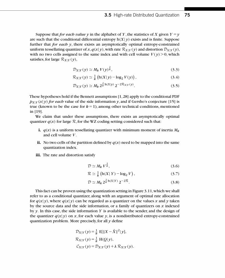
3.5 High-rate Distributed Quantization 75
Suppose that for each value y in the alphabet of Y , the statistics of X given Y �yare such that the conditional differential entropy h(X | y) exists and is finite. Supposefurther that for each y, there exists an asymptotically optimal entropy-constraineduniform tessellating quantizer of x,q(x| y),with rate RX |Y (y) and distortion DX |Y (y),with no two cells assigned to the same index and with cell volume V ( y)�0, whichsatisfies, for large RX |Y (y),
DX |Y (y) � Mk V (y)2k , (3.3)
RX |Y (y) � 1k
(h(X | y)� log2 V (y)
), (3.4)
DX |Y (y) � Mk 22k h(X |y) 2�2RX |Y (y). (3.5)
These hypotheses hold if the Bennett assumptions [1,28] apply to the conditional PDFpX |Y (x| y) for each value of the side information y, and if Gersho’s conjecture [15] istrue (known to be the case for k�1), among other technical conditions, mentionedin [19].
We claim that under these assumptions, there exists an asymptotically optimalquantizer q(x) for large R, for the WZ coding setting considered such that:
i. q(x) is a uniform tessellating quantizer with minimum moment of inertia Mk
and cell volume V .
ii. No two cells of the partition defined by q(x) need to be mapped into the samequantization index.
iii. The rate and distortion satisfy
D � Mk V2k , (3.6)
R � 1k
(h(X |Y )� log2 V
), (3.7)
D � Mk 22k h(X |Y ) 2�2R. (3.8)
This fact can be proven using the quantization setting in Figure 3.11,which we shallrefer to as a conditional quantizer, along with an argument of optimal rate allocationfor q(x| y), where q(x| y) can be regarded as a quantizer on the values x and y takenby the source data and the side information, or a family of quantizers on x indexedby y. In this case, the side information Y is available to the sender, and the design ofthe quantizer q(x| y) on x, for each value y, is a nondistributed entropy-constrainedquantization problem. More precisely, for all y define
DX |Y (y)� 1k E[‖X � X‖2| y],
RX |Y (y)� 1k H(Q| y),
CX |Y (y)�DX |Y (y)�� RX |Y (y).

76 CHAPTER 3 Quantization for Distributed Source Coding
|q (x y ) x (q, y )ˆX Q X
Y
FIGURE 3.11
Conditional quantizer.
By iterated expectation, D�E DX |Y (Y ) and R�E RX |Y (Y ); thus the overall costsatisfies C �E CX |Y (Y ). As a consequence, a family of quantizers q(x| y) minimizingCX |Y (y) for each y also minimizes C.
Since CX |Y (y) is a convex function of RX |Y (y) for all y, it has a global minimumwhere its derivative vanishes,or equivalently,at RX |Y (y) such that ��2 ln 2 DX |Y (y).Suppose that � is small enough for RX |Y (y) to be large and for the approximations(3.3)–(3.5) to hold, for each y.Then,all quantizers q(x| y) introduce the same distortion(proportional to �) and consequently have a common cell volume V (y)�V . This,together with the fact that EY [h(X | y)]y�Y �h(X |Y ), implies (3.6)–(3.8). Providedthat a translation of the partition defined by q(x| y) affects neither the distortion northe rate,all uniform tessellating quantizers q(x| y) may be set to be (approximately) thesame, which we denote by q(x). Since none of the quantizers q(x| y) maps two cellsinto the same indices, neither does q(x). Now, since q(x) is asymptotically optimalfor the conditional quantizer and does not depend on y, it is also optimal for the WZquantizer in Figure 3.10. This proves our claim.
We would like to remark that Equation (3.8) means that, asymptotically, there is noloss in performance by not having access to the side information in the quantization.In addition,since index repetition is not required,the distortion (3.6) would be asymp-totically the same if the reconstruction x(q, y) were of the form x(q)�E[X | q]. Thismeans that under the hypotheses of this section,asymptotically,there is a quantizer thatleads to no loss in performance by ignoring the side information in the reconstruction(but it is still used by the SW decoder).
Finally, let X and Y be jointly Gaussian random vectors. Recall that the conditionalcovariance X |Y does not depend on y, that h(X |Y )� 1
2 log2
((2�e)k det X |Y
), and
that Mk→ 12�e [49]. Then, on account of the results of this section, for large R,
D � Mk 2�e (det X |Y )1k 2�2R �→[k→�] (det X |Y )
1k 2�2R. (3.9)
3.5.2 High-rate WZ Quantization of Noisy Sources
We will now examine the properties of high-rate quantizers of a noisy source with sideinformation at the decoder, as illustrated in Figure 3.12, which we will refer to as WZ

3.5 High-rate Distributed Quantization 77
SWEncoder
Q QSW
Decoder x (q, y )X
Y
Encoder withoutSide Information
Decoder withSide Information
q (z )Z ˆ
ˆ
FIGURE 3.12
WZ quantization of a noisy source.
q (z )Z Q X
x (q)ˆˆ
FIGURE 3.13
Quantization of a noisy source without side information.
quantizers of a noisy source.This is precisely the network in Section 3.2.2 with m�1encoders and n�1 decoders. Unlike the problem in Section 3.5.1, this time a noisyobservation Z is quantized in lieu of the unseen source data X . Clearly, this includesthe problem in the previous section as the particular case Z �X .
The hypotheses of the previous section directly carry over to the more generalproblem studied here. Assume that X takes values in R
k. The expected distortion persample of the unseen source is defined as D� 1
k E ‖X � X‖2. Suppose further thatthe coding of the index Q is carried out by an ideal SW coder, at a rate per sampleR� 1
k H(Q|Y ). We emphasize that the quantizer only has access to the observation,not to the source data or the side information. However, the joint statistics of X , Y ,and Z can be exploited in the design of q(z) and x(q, y). Consistently withSection 3.2.4, we consider the problem of characterizing the quantizers and recon-struction functions that minimize the expected Lagrangian cost C �D��R, with � anonnegative real number, for high-rate R.
3.5.2.1 Nondistributed CaseWe start by considering the simpler case of quantization of a noisy source without sideinformation,depicted in Figure 3.13.The following extends the main result of [10,41]to entropy-constrained quantization,valid for any rate R�H(Q),not necessarily high.
Define x(z)�E[X | z], the best MSE estimator of X given Z ,and X � x(Z).We showin [32, 35] that for any nonnegative � and any Lagrangian-cost optimal quantizer of anoisy source without side information (Figure 3.13), there exists an implementationwith the same cost in two steps:

78 CHAPTER 3 Quantization for Distributed Source Coding
q (x )X Q X
E[X u z ]Z ˆ
x (q )ˆ
FIGURE 3.14
Optimal implementation of MSE quantization of a noisy source without side information.
1. Obtain the minimum MSE estimate X .
2. Quantize the estimate X regarded as a clean source,using a quantizer q(x) anda reconstruction function x(q), minimizing E ‖X � X‖2 �� H(Q).
This is illustrated in Figure 3.14. Furthermore, the total distortion per sample is
D� 1k
(E tr Cov[X |Z]�E ‖X � X‖2), (3.10)
where the first term is the MSE of the estimation step.The following observation is an immediate consequence of the previous,very intui-
tive result,and conventional theory of high-rate quantization of clean sources.Assumenow that h(X)�� and that there exists a uniform tessellating quantizer q(x) of Xwith cell volume V that is asymptotically optimal in Lagrangian cost at high rates.Then, there exists an asymptotically optimal quantizer q(z) of a noisy source in thesetting of Figure 3.13 such that:
i. An asymptotically optimal implementation of q(z) is that representedin Figure 3.14, with a uniform tessellating quantizer q(x) having cellvolume V .
ii. The rate and distortion per sample satisfy
D� 1k E tr Cov[X |Z]�Mk V
2k ,
R� 1k
(h(X)� log2 V
),
D� 1k E tr Cov[X |Z]�Mk 2
2k h(X) 2�2R.
3.5.2.2 Distributed CaseWe are now ready to consider WZ quantization of a noisy source, as shown inFigure 3.12. Define x(y, z)�E[X | y, z], the best MSE estimator of X given Y and Z ,X � x(Y , Z), and D� � 1
k E tr Cov[X |Y , Z]. The following fact is an extension of theresults on high-rate WZ quantization in Section 3.5, to noisy sources.
Suppose that the conditional expectation function x(y, z) is additively separable,that is, x(y, z)� xY (y)� xZ (z), and define XZ � xZ (Z). Suppose further that for eachvalue y in the alphabet of Y , h(X | y)��, and that there exists a uniform tessellatingquantizer q(x, y) of X , with no two cells assigned to the same index and cell volumeV (y)�0, with rate RX |Y (y) and distortion DX |Y (y), such that, at high rates, it is

3.5 High-rate Distributed Quantization 79
asymptotically optimal in Lagrangian cost and
DX |Y (y)�Mk V (y)2k ,
RX |Y (y)� 1k
(h(X | y)� log2 V (y)
),
DX |Y (y)�Mk 22k h(X |y) 2�2RX |Y (y)
.
It was proved in [35,36] that under these assumptions there exists an asymptoticallyoptimal quantizer q(z) for large R, for the WZ quantization setting represented inFigure 3.12, such that:
i. q(z) can be implemented as an estimator xZ (z) followed by a uniformtessellating quantizer q(xZ ) with cell volume V .
ii. No two cells of the partition defined by q(xZ ) need to be mapped into thesame quantization index.
iii. The rate and distortion per sample satisfy
D�D� �Mk V2k , (3.11)
R� 1k
(h(X |Y )� log2 V
), (3.12)
D�D� �Mk 22k h(X |Y ) 2�2R. (3.13)
iv. h(X |Y )�h(XZ |Y ).
Clearly, this is a generalization of the clean case in Section 3.5.1, since Z �X impliesx(y, z)� xZ (z)�z, trivially additively separable. Observe that, if the estimator x(y, z)
is additively separable, there is no asymptotic loss in performance by not using theside information at the encoder.
The proof of this fact is very similar to that for clean sources in Section 3.5.1.More precisely, it analyzes the case when the side information is available at theencoder. The main difference is that it applies the separation result obtained for thenoisy, nondistributed case, to the noisy, conditional setting, for each value of the sideinformation.
The case in which X can be written as X � f (Y )�g(Z)�N , for any (measur-able) functions f , g and any random variable N with E[N | y, z] constant with (y, z),gives an example of an additively separable estimator. This includes the case inwhich X , Y , and Z are jointly Gaussian. Furthermore, in the Gaussian case, sincexZ (z) is an affine function and q(xZ ) is a uniform tessellating quantizer, the over-all quantizer q(xZ (z)) is also a uniform tessellating quantizer, and if Y and Z areuncorrelated, then xY (y)�E[X | y] and xZ (z)�E[X | z], which does not hold ingeneral.
Similarly to the observation made in the clean case, there is a WZ quantizer q(xZ )
that leads to no asymptotic loss in performance if the reconstruction function is
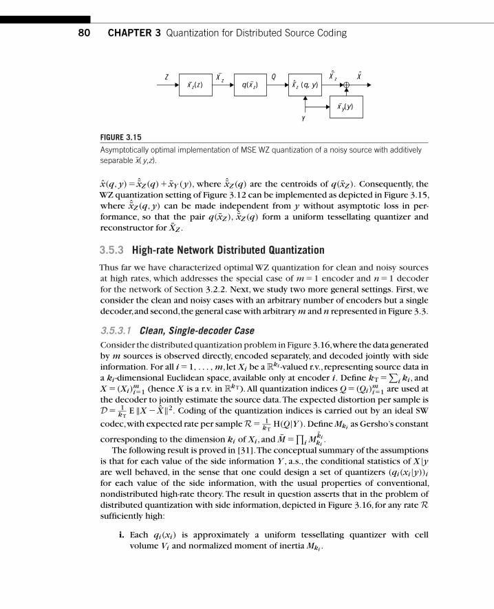
80 CHAPTER 3 Quantization for Distributed Source Coding
ˆQ
xy(y)
xz (q, y)q (xz)Z
Y
XXz ˆ ˆ
x z(z)Xz
FIGURE 3.15
Asymptotically optimal implementation of MSE WZ quantization of a noisy source with additivelyseparable x( y,z).
x(q, y)� ˆxZ (q)� xY (y), where ˆxZ (q) are the centroids of q(xZ ). Consequently, theWZ quantization setting of Figure 3.12 can be implemented as depicted in Figure 3.15,where ˆxZ (q, y) can be made independent from y without asymptotic loss in per-formance, so that the pair q(xZ ), ˆxZ (q) form a uniform tessellating quantizer andreconstructor for XZ .
3.5.3 High-rate Network Distributed Quantization
Thus far we have characterized optimal WZ quantization for clean and noisy sourcesat high rates, which addresses the special case of m�1 encoder and n�1 decoderfor the network of Section 3.2.2. Next, we study two more general settings. First, weconsider the clean and noisy cases with an arbitrary number of encoders but a singledecoder,and second,the general case with arbitrary m and n represented in Figure 3.3.
3.5.3.1 Clean, Single-decoder CaseConsider the distributed quantization problem in Figure 3.16,where the data generatedby m sources is observed directly, encoded separately, and decoded jointly with sideinformation. For all i �1, . . . , m, let Xi be a R
ki -valued r.v., representing source data ina ki -dimensional Euclidean space, available only at encoder i. Define kT �
∑i ki , and
X �(Xi)mi�1 (hence X is a r.v. in R
kT). All quantization indices Q�(Qi)mi�1 are used at
the decoder to jointly estimate the source data.The expected distortion per sample isD� 1
kTE ‖X � X‖2. Coding of the quantization indices is carried out by an ideal SW
codec,with expected rate per sample R� 1kT
H(Q|Y ). Define Mki as Gersho’s constant
corresponding to the dimension ki of Xi , and M �∏
i Mkiki
.The following result is proved in [31].The conceptual summary of the assumptions
is that for each value of the side information Y , a.s., the conditional statistics of X |yare well behaved, in the sense that one could design a set of quantizers (qi(xi|y))i
for each value of the side information, with the usual properties of conventional,nondistributed high-rate theory. The result in question asserts that in the problem ofdistributed quantization with side information,depicted in Figure 3.16, for any rate Rsufficiently high:
i. Each qi(xi) is approximately a uniform tessellating quantizer with cellvolume Vi and normalized moment of inertia Mki .
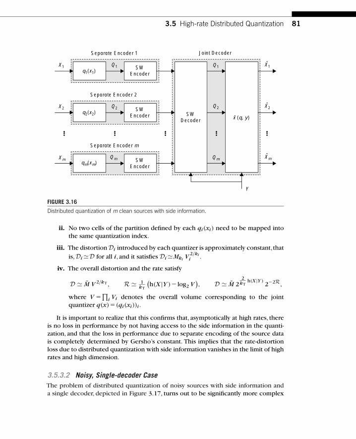
3.5 High-rate Distributed Quantization 81
SWEncoder SW
Decoder
Separate Encoder 1 Joint Decoder
Separate Encoder 2
X1
Xm
X2q2(x2)
q1(x1)
x (q, y )
Xm
Separate Encoder m
Qm
Q1
Q2 Q2
Qm
Q1
Y
qm(xm)
SWEncoder
SWEncoder
ˆ
X2ˆ
X1ˆ
ˆ
FIGURE 3.16
Distributed quantization of m clean sources with side information.
ii. No two cells of the partition defined by each qi(xi) need to be mapped intothe same quantization index.
iii. The distortion Di introduced by each quantizer is approximately constant,that
is,Di�D for all i, and it satisfies Di�Mki V 2/kii .
iv. The overall distortion and the rate satisfy
D � M V 2/kT , R � 1kT
(h(X |Y )� log2 V
), D � M 2
2kT
h(X |Y )2�2R,
where V �∏
i Vi denotes the overall volume corresponding to the jointquantizer q(x)�(qi(xi))i .
It is important to realize that this confirms that, asymptotically at high rates, thereis no loss in performance by not having access to the side information in the quanti-zation, and that the loss in performance due to separate encoding of the source datais completely determined by Gersho’s constant. This implies that the rate-distortionloss due to distributed quantization with side information vanishes in the limit of highrates and high dimension.
3.5.3.2 Noisy, Single-decoder CaseThe problem of distributed quantization of noisy sources with side information anda single decoder, depicted in Figure 3.17, turns out to be significantly more complex

82 CHAPTER 3 Quantization for Distributed Source Coding
SWEncoder SW
Decoder
Separate Encoder 1 Joint Decoder
Separate Encoder 2
SWEncoder
Z1
Zm
Z2q2(z2)
q1(z1)
X
x (q, y)
SWEncoder
Separate Encoder m
Qm
Q1
Q2 Q2
Qm
Q1
Y
qm(zm)
ˆ
ˆ
FIGURE 3.17
Distributed quantization of m noisy sources with side information.
when several encoders are involved. In fact, the analysis developed in [31] builds onthe special case when the source data is the sum of the observations,in such a way thatthe clean case is no longer a special case of the noisy one, except for the WZ setting,that is, when m�1. The argument considers transformations of the observations thatpreserve optimal performance,conceptually not too distant from the separation resultfor noisy,nondistributed quantization,described in Section 3.5.2,albeit mathematicallymore sophisticated. Here, we present the main result.
As usual, X is a Rk-valued r.v. We define D� � 1
k E tr Cov[X |Y , Z]. First, we makethe following assumptions on the statistical dependence of X , Y , and Z :
i. There exist measurable functions xY :Y→Rk and xZi :Zi→R
k, i �1, . . . , m,such that E[X |y, z]� xY (y)�
∑i xZi (zi). Define XY � xY (Y ) and XZi � xZi (Zi),
thus X � XY �∑
i XZi .
ii. Either m�1, or {Zi}i are conditionally independent given Y , or the maps{x → xZi (x)}i are injective.
Furthermore, it is assumed that for almost every y∈Y , the conditional statistics of(XZi )i|y are well-behaved, in the sense of conventional, nondistributed high-ratequantization theory.

3.5 High-rate Distributed Quantization 83
Under these assumptions, in the problem of noisy distributed quantization withside information, depicted in Figure 3.17, for any rate R sufficiently high:
i. There exists a collection of asymptotically optimal quantizers (qi(zi))i , con-sisting of the transformations (xZi (zi))i , followed by approximately uniformtessellating quantizers with a common cell volume V 1/m and normalizedmoment of inertia Mk, where V represents the volume of the correspondingjoint tessellation.
ii. No two cells of the partition defined by each qi(zi) need to be mapped intothe same quantization index.
iii. The overall distortion and the rate satisfy
D�D� �D,
1m D�Mk V
2km ,
1mR� 1
km
(h((XZi )
mi�1|Y )� log2 V
),
1m D�Mk 2
2km h((XZi )
mi�1|Y ) 2�2 1
m R.
3.5.3.3 Network CaseOur final high-rate analysis is concerned with the general problem of network dis-tributed quantization of noisy sources with side information,presented in Section 3.2.2and depicted in Figure 3.3. We assume that it is possible to break down the networkinto n∈Z
� subnetworks such that:
i. The overall distortion D is a nonnegative linear combination of the distortionsDj of each subnetwork,and the overall rate R is a positive linear combination ofthe rates Rj of each subnetwork. Mathematically,D�
∑j �jDj and R�
∑j jRj ,
for some �j, j ∈R�.
ii. For each subnetwork j, the distortion and rate are (approximately) related byan exponential law of the form Dj �D� j �Dj ,where Dj ��j 2�Rj/�j , for someD� j ∈R and �j, �j ∈R
�.
The first assumption holds, for example, when the overall distortion for the networkdistributed codec is a nonnegative linear combination of distortions correspondingto reconstructions at each decoder, and ideal SW codecs are used for lossless cod-ing of the quantization indices. The second assumption holds approximately for eachof the high-rate quantization problems studied in this section, including the compli-cated exponential law for the rate-distortion performance in the single-decoder noisynetwork, which did not obey the 6 dB/bit rule. Simply speaking, these assumptionsmean that we can basically break down a network distributed coding problem intosubproblems that satisfy the hypotheses of the cases considered thus far.

84 CHAPTER 3 Quantization for Distributed Source Coding
The next result characterizes the overall rate-distortion performance of the networkdistributed codec by means of an optimal rate allocation. Specifically,we consider theproblem of minimizing D subject to a constraint on R. We would like to remark thatalthough it is possible to incorporate nonnegativity constraints on each of the rates Rj
into the problem, and to solve it using the Karush–Kuhn–Tucker (KKT) conditions,our second assumption makes the result practical only at high rates, which implicitlyintroduce nonnegativity.
Define
D� �∑
j
�jD� j, D�∑
j
�jDj,
��∑
j
�jj �0, and ���∏
j
(�j�j
�jj
)�j j�
�0.
It is clear that D�D� �D. It can be shown [31] that the minimum D subject to aconstraint on R is given by
D�� 2�R/�. (3.14)
Furthermore, the minimum is achieved if, and only if,
Dj ��jj
��jD, (3.15)
or equivalently,
Rj
�j�
R�
� log2�j��j
��jj. (3.16)
Observe that the overall rate-distortion performance of the network distributed codecfollows the same exponential law of each of the subnetworks, which permits a hier-archical application, considering networks of networks when convenient. This doesnot come as a surprise since a common principle lies behind all of our high-ratequantization proofs: a rate allocation problem where rate and distortion are relatedexponentially.
3.6 EXPERIMENTAL RESULTS REVISITEDIn this section we proceed to revisit the experimental results of Section 3.4,where theLloyd algorithm described in Section 3.3.2 was applied to a scalar, quadratic-GaussianWZ coding problem. Precisely, X∼N (0, 1) and NY ∼N (0, 1/10) were independent,and Y �X �NY .
We saw in Section 3.5.1 that the high-rate approximation to the operational dis-tortion-rate function is given by (3.9). Figure 3.6, which showed the rate-distortion
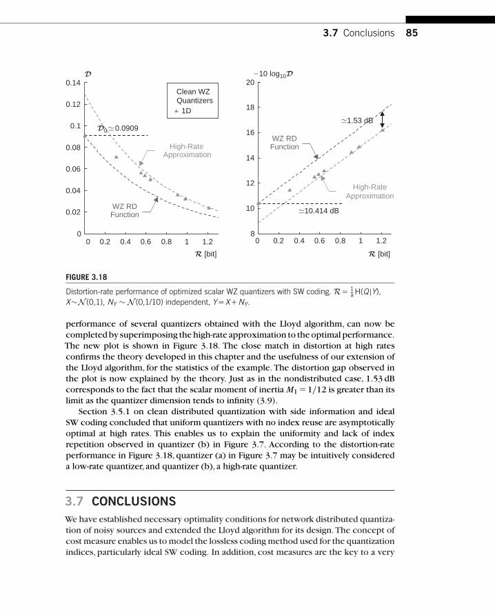
3.7 Conclusions 85
0 0.2 0.4 0.6 0.8 1 1.2 0 0.2 0.4 0.6 0.8 1 1.20
0.02
0.04
0.06
0.08
0.1
0.12
0.14Clean WZQuantizers
1D
8
10
12
14
16
18
20
R [bit]R [bit]
D
WZ RD Function
High-Rate Approximation
�1.53 dB
�10.414 dB
210 log10D
D0�0.0909
High-RateApproximation
WZ RD Function
FIGURE 3.18
Distortion-rate performance of optimized scalar WZ quantizers with SW coding. R� 1k H(Q |Y),
X∼N (0,1), NY ∼ N (0,1/10) independent, Y�X�NY.
performance of several quantizers obtained with the Lloyd algorithm, can now becompleted by superimposing the high-rate approximation to the optimal performance.The new plot is shown in Figure 3.18. The close match in distortion at high ratesconfirms the theory developed in this chapter and the usefulness of our extension ofthe Lloyd algorithm, for the statistics of the example. The distortion gap observed inthe plot is now explained by the theory. Just as in the nondistributed case, 1.53 dBcorresponds to the fact that the scalar moment of inertia M1 �1/12 is greater than itslimit as the quantizer dimension tends to infinity (3.9).
Section 3.5.1 on clean distributed quantization with side information and idealSW coding concluded that uniform quantizers with no index reuse are asymptoticallyoptimal at high rates. This enables us to explain the uniformity and lack of indexrepetition observed in quantizer (b) in Figure 3.7. According to the distortion-rateperformance in Figure 3.18, quantizer (a) in Figure 3.7 may be intuitively considereda low-rate quantizer, and quantizer (b), a high-rate quantizer.
3.7 CONCLUSIONSWe have established necessary optimality conditions for network distributed quantiza-tion of noisy sources and extended the Lloyd algorithm for its design. The concept ofcost measure enables us to model the lossless coding method used for the quantizationindices, particularly ideal SW coding. In addition, cost measures are the key to a very
86 CHAPTER 3 Quantization for Distributed Source Coding
general formulation that unifies a number of related problems, such as broadcast withside information, distributed classification, or quantization of side information.
If ideal SW coders are used, uniform tessellating quantizers without index repe-tition are asymptotically optimal at high rates. It is known [47] that the rate loss inthe WZ problem for smooth continuous sources and quadratic distortion vanishes asD→0. Our work shows that this is also true for the operational rate loss and for eachfinite dimension k. These approximations have been applied to develop a theory oftransforms for distributed source coding, which assumes high rates [32, 35], but notarbitrarily high dimension or Gaussian statistics [13, 14].
Suppose that the conditional expectation of the unseen source data X given the sideinformation Y and the noisy observation Z is additively separable.Then, at high rates,optimal WZ quantizers of Z can be decomposed into estimators and uniform tessel-lating quantizers for clean sources, achieving the same rate-distortion performanceas if the side information were available at the encoder. The additive separabilitycondition for high-rate WZ quantization of noisy sources, albeit less restrictive, issimilar to the condition required for zero rate loss in the quadratic Gaussian noisyWZ problem [33], which applies exactly for any rate but requires arbitrarily largedimension.
Experimental results confirm the high-rate approximation theory for distributedquantization. In addition,they suggest that the convergence properties of the extendedLloyd algorithm are similar to those of the classical one and can benefit from a geneticsearch algorithm for initialization.
REFERENCES[1] W. R. Bennett,“Spectra of quantized signals,”Bell Syst., Tech. J. 27, July 1948.
[2] J.A. Bucklew and G. L.Wise,“Multidimensional asymptotic quantization theory with rth powerdistortion measures,” IEEE Trans. Inform.Theory, vol. IT-28, pp. 239–247, Mar. 1982.
[3] J. Cardinal,“Compression of side information,” in Proc.IEEE Int.Conf. Multimedia, Expo (ICME),vol. 2, Baltimore, MD, July 2003, pp. 569–572.
[4] ,“Quantization of side information,”unpublished.
[5] J. Cardinal and G.V.Asche,“Joint entropy-constrained multiterminal quantization,”in Proc. IEEEInt. Symp. Inform.Theory (ISIT), Lausanne, Switzerland, June 2002, p. 63.
[6] T. M. Cover, “A proof of the data compression theorem of Slepian andWolf for ergodic sources,”IEEE Trans. Inform.Theory, vol. 21, no. 2, pp. 226–228, Mar. 1975, (Corresp.).
[7] I. Csiszár, “Generalized entropy and quantization problems,” in Proc. Prague Conf. Inform.Theory, Stat. Decision Functions, Random Processes, Prague, Czech Republic, 1973,pp. 159–174.
[8] R. L. Dobrushin and B. S.Tsybakov,“Information transmission with additional noise,”IRE Trans.Inform.Theory, vol. IT-8, pp. S293–S304, 1962.
[9] M. Effros and D. Muresan,“Codecell contiguity in optimal fixed-rate and entropy-constrainednetwork scalar quantizers,” in Proc. IEEE Data Compression Conf. (DCC), Snowbird, UT,Apr. 2002, pp. 312–321.
[10] Y. Ephraim and R. M. Gray,“A unified approach for encoding clean and noisy sources by meansof waveform and autoregressive vector quantization,” IEEE Trans. Inform. Theory, vol. IT-34,pp. 826–834, July 1988.

References 87
[11] M. Fleming and M. Effros,“Network vector quantization,”in Proc.IEEE Data Compression Conf.(DCC), Snowbird, UT, Mar. 2001, pp. 13–22.
[12] M. Fleming, Q. Zhao, and M. Effros,“Network vector quantization,” IEEE Trans. Inform.Theory,vol. 50, no. 8, pp. 1584–1604, Aug. 2004.
[13] M. Gastpar, P. L. Dragotti, and M. Vetterli, “The distributed Karhunen-Loève transform,” IEEETrans. Inform.Theory, 2004, submitted for publication.
[14] , “On compression using the distributed Karhunen–Loève transform,” in Proc. IEEEInt. Conf. Acoust., Speech, Signal Processing (ICASSP), vol. 3, Montréal, Canada, May 2004,pp. 901–904.
[15] A. Gersho,“Asymptotically optimal block quantization,” IEEE Trans. Inform.Theory, vol. IT-25,pp. 373–380, July 1979.
[16] A. Gersho and R. M. Gray, Vector Quantization and Signal Compression. Boston, MA: KluwerAcademic Publishers, 1992.
[17] H. Gish and J. N. Pierce, “Asymptotically efficient quantizing,” IEEE Trans. Inform. Theory,vol. IT-14, pp. 676–683, Sept. 1968.
[18] R. M. Gray, T. Linder, and J. Li, “A Lagrangian formulation of Zador’s entropy-constrainedquantization theorem,” IEEE Trans. Inform.Theory, vol. 48, no. 3, pp. 695–707, March 2002.
[19] R. M. Gray and D. L. Neuhoff, “Quantization,” IEEE Trans. Inform. Theory, vol. 44,pp. 2325–2383, Oct. 1998.
[20] J.A. Gubner,“Distributed estimation and quantization,”IEEE Trans.Inform.Theory,vol. 39,no. 4,pp. 1456–1459, July 1993.
[21] J. Kusuma, L. Doherty, and K. Ramchandran, “Distributed compression for sensor networks,”in Proc. IEEE Int. Conf. Image Processing (ICIP), vol. 1, Thessaloniki, Greece, Oct. 2001,pp. 82–85.
[22] W. M. Lam and A. R. Reibman, “Quantizer design for decentralized estimation systems withcommunication constraints,”in Proc. Annual Conf. Inform.Sci.Syst. (CISS),Baltimore,MD,Mar.1989.
[23] ,“Design of quantizers for decentralized estimation systems,”IEEE Trans.Inform.Theory,vol. 41, no. 11, pp. 1602–1605, Nov. 1993.
[24] T. Linder and K. Zeger,“Asymptotic entropy-constrained performance of tessellating and uni-versal randomized lattice quantization,” IEEE Trans. Inform.Theory, vol. 40, pp. 575–579, Mar.1993.
[25] Z. Liu,S. Cheng, A. D. Liveris,and Z. Xiong,“Slepian–Wolf coded nested quantization (SWC-NQ)for Wyner-Ziv coding:Performance analysis and code design,” in Proc. IEEE Data CompressionConf. (DCC), Snowbird, UT, Mar. 2004, pp. 322–331.
[26] S. P. Lloyd, “Least squares quantization in PCM,” IEEE Trans. Inform. Theory, vol. IT-28,pp. 129–137, Mar. 1982.
[27] D. Muresan and M. Effros, “Quantization as histogram segmentation: Globally optimal scalarquantizer design in network systems,”in Proc. IEEE Data Compression Conf.(DCC), Snowbird,UT, Apr. 2002, pp. 302–311.
[28] S. Na and D. L. Neuhoff,“Bennett’s integral for vector quantizers,” IEEE Trans. Inform.Theory,vol. 41, pp. 886–900, July 1995.
[29] S. S. Pradhan, J. Kusuma,and K. Ramchandran,“Distributed compression in a dense microsensornetwork,” IEEE Signal Processing Mag., vol. 19, pp. 51–60, Mar. 2002.
[30] S. S. Pradhan and K. Ramchandran, “Distributed source coding using syndromes (DISCUS):Design and construction,” in Proc. IEEE Data Compression Conf. (DCC), Snowbird, UT, Mar.1999, pp. 158–167.
[31] D. Rebollo-Monedero, “Quantization and transforms for distributed source coding,” Ph.D.dissertation, Stanford Univ., 2007.

88 CHAPTER 3 Quantization for Distributed Source Coding
[32] D. Rebollo-Monedero, A. Aaron, and B. Girod, “Transforms for high-rate distributed sourcecoding,” in Proc. Asilomar Conf. Signals, Syst., Comput., vol. 1, Pacific Grove, CA, Nov. 2003,pp. 850–854, invited paper.
[33] D. Rebollo-Monedero and B. Girod,“A generalization of the rate-distortion function for Wyner–Ziv coding of noisy sources in the quadratic-Gaussian case,” in Proc. IEEE Data CompressionConf. (DCC), Snowbird, UT, Mar. 2005, pp. 23–32.
[34] , “Network distributed quantization,” in Proc. IEEE Inform. Theory Workshop (ITW),Lake Tahoe, CA, Sept. 2007, invited paper.
[35] D. Rebollo-Monedero, S. Rane, A. Aaron, and B. Girod, “High-rate quantization and transformcoding with side information at the decoder,” EURASIP J. Signal Processing, Special IssueDistrib. Source Coding, vol. 86, no. 11, pp. 3160–3179, Nov. 2006, invited paper.
[36] D. Rebollo-Monedero, S. Rane, and B. Girod, “Wyner–Ziv quantization and transform codingof noisy sources at high rates,” in Proc. Asilomar Conf. Signals, Syst., Comput., vol. 2, PacificGrove, CA, Nov. 2004, pp. 2084–2088.
[37] D. Rebollo-Monedero, R. Zhang, and B. Girod, “Design of optimal quantizers for distributedsource coding,” in Proc. IEEE Data Compression Conf. (DCC), Snowbird, UT, Mar. 2003,pp. 13–22.
[38] S. D. Servetto,“Lattice quantization with side information,” in Proc. IEEE Data CompressionConf. (DCC), Snowbird, UT, Mar. 2000, pp. 510–519.
[39] J. D. Slepian and J. K. Wolf,“Noiseless coding of correlated information sources,” IEEE Trans.Inform.Theory, vol. IT-19, pp. 471–480, July 1973.
[40] H.Viswanathan,“Entropy coded tesselating quantization of correlated sources is asymptoticallyoptimal,”1996, unpublished.
[41] J. K. Wolf and J. Ziv, “Transmission of noisy information to a noisy receiver with minimumdistortion,” IEEE Trans. Inform.Theory, vol. IT-16, no. 4, pp. 406–411, July 1970.
[42] A. D. Wyner and J. Ziv,“The rate-distortion function for source coding with side information atthe decoder,” IEEE Trans. Inform.Theory, vol. IT-22, no. 1, pp. 1–10, Jan. 1976.
[43] Z. Xiong, A. Liveris, S. Cheng, and Z. Liu, “Nested quantization and Slepian–Wolf coding:AWyner–Ziv coding paradigm for i.i.d. sources,”in Proc.IEEEWorkshop Stat.Signal Processing(SSP), St. Louis, MO, Sept. 2003, pp. 399–402.
[44] Z. Xiong, A. D. Liveris, and S. Cheng, “Distributed source coding for sensor networks,” IEEESignal Processing Mag., vol. 21, no. 5, pp. 80–94, Sept. 2004.
[45] Y. Yang, S. Cheng, Z. Xiong, and W. Zhao, “Wyner–Ziv coding based on TCQ and LDPCcodes,” in Proc. Asilomar Conf. Signals, Syst., Comput., vol. 1, Pacific Grove, CA, Nov. 2003,pp. 825–829.
[46] P. L. Zador, “Asymptotic quantization error of continuous signals and the quantizationdimension,” IEEE Trans. Inform.Theory, vol. IT-28, no. 2, pp. 139–149, Mar. 1982.
[47] R. Zamir,“The rate loss in the Wyner–Ziv problem,” IEEE Trans. Inform.Theory, vol. 42, no. 6,pp. 2073–2084, Nov. 1996.
[48] R. Zamir and T. Berger, “Multiterminal source coding with high resolution,” IEEE Trans.Inform.Theory, vol. 45, no. 1, pp. 106–117, Jan. 1999.
[49] R. Zamir and M. Feder,“On lattice quantization noise,”IEEE Trans.Inform.Theory,vol. 42,no. 4,pp. 1152–1159, July 1996.
[50] R. Zamir and S. Shamai, “Nested linear/lattice codes for Wyner–Ziv encoding,” in Proc. IEEEInform.Theory Workshop (ITW), Killarney, Ireland, June 1998, pp. 92–93.
[51] R. Zamir, S. Shamai, and U. Erez, “Nested linear/lattice codes for structured multiterminalbinning,” IEEE Trans. Inform.Theory, vol. 48, no. 6, pp. 1250–1276, June 2002.
CHAPTER
4Zero-error Distributed SourceCoding
Ertem TuncelDepartment of Electrical Engineering, University of California, Riverside, CA
Jayanth NayakMayachitra, Inc., Santa Barbara, CA
Prashant Koulgi and Kenneth RoseDepartment of Electrical and Computer Engineering, University of California,
Santa Barbara, CA
C H A P T E R C O N T E N T SIntroduction . . . . . . . . . . . . . . . . . . . . . . . . . . . . . . . . . . . . . . . . . . . . . . . . . . . . . . . . . . . . . . . . . . . . . . . . . . . . . . 89Graph Theoretic Connections . . . . . . . . . . . . . . . . . . . . . . . . . . . . . . . . . . . . . . . . . . . . . . . . . . . . . . . . . . . . 92
VLZE Coding and Graphs. . . . . . . . . . . . . . . . . . . . . . . . . . . . . . . . . . . . . . . . . . . . . . . . . . . . . . . . . . . 92Basic Definitions and Notation. . . . . . . . . . . . . . . . . . . . . . . . . . . . . . . . . . . . . . . . . . . . . . . . . . . . . 95Graph Entropies . . . . . . . . . . . . . . . . . . . . . . . . . . . . . . . . . . . . . . . . . . . . . . . . . . . . . . . . . . . . . . . . . . . . 96Graph Capacity . . . . . . . . . . . . . . . . . . . . . . . . . . . . . . . . . . . . . . . . . . . . . . . . . . . . . . . . . . . . . . . . . . . . . 98
Complementary Graph Entropy and VLZE Coding . . . . . . . . . . . . . . . . . . . . . . . . . . . . . . . . . . . . . . . . 98Network Extensions . . . . . . . . . . . . . . . . . . . . . . . . . . . . . . . . . . . . . . . . . . . . . . . . . . . . . . . . . . . . . . . . . . . . . . 100
Extension 1: VLZE Coding When Side Information May Be Absent . . . . . . . . . . . . . . . . 100Extension 2: VLZE Coding with Compound Side Information . . . . . . . . . . . . . . . . . . . . . . 102
VLZE Code Design . . . . . . . . . . . . . . . . . . . . . . . . . . . . . . . . . . . . . . . . . . . . . . . . . . . . . . . . . . . . . . . . . . . . . . . 104Hardness of Optimal Code Design . . . . . . . . . . . . . . . . . . . . . . . . . . . . . . . . . . . . . . . . . . . . . . . . . 104Hardness of Coding with Length Constraints . . . . . . . . . . . . . . . . . . . . . . . . . . . . . . . . . . . . . . . 107An Exponential-time Optimal VLZE Code Design Algorithm .. . . . . . . . . . . . . . . . . . . . . . 108
Conclusions . . . . . . . . . . . . . . . . . . . . . . . . . . . . . . . . . . . . . . . . . . . . . . . . . . . . . . . . . . . . . . . . . . . . . . . . . . . . . . 109References . . . . . . . . . . . . . . . . . . . . . . . . . . . . . . . . . . . . . . . . . . . . . . . . . . . . . . . . . . . . . . . . . . . . . . . . . . . . . . . 110
4.1 INTRODUCTIONThis chapter tackles the classical distributed source coding (DSC) problem from a dif-ferent perspective.As usual, let Xn and Y n be a pair of correlated sequences observed
Distributed Source Coding: Theory, Algorithms, and ApplicationsCopyright © 2008 by Academic Press, Inc. All rights of reproduction in any form reserved. 89

90 CHAPTER 4 Zero-error Distributed Source Coding
by two sensors SX and SY . Also, let the samples (Xt , Yt)∈X �Y be i.i.d.∼PXY (x, y),where without loss of generality, it can be assumed that PX (x)�0 and PY ( y)�0 forall (x, y)∈X �Y . The sensors are required to convey these sequences to SZ , a thirdsensor or a central processing unit, without communicating with each other. Whatis the region of achievable rates RX and RY if the reconstruction (Xn, Y n) at SZ isto be lossless? The answer heavily depends on what is meant by “lossless,” as well ason whether or not we are allowed to use variable-length codes. More specifically, thesensors could be operating under three different requirements, which are listed herein increasing order of strength:
a. Coding with vanishingly small error: This is the original DSC regime asintroduced by Slepian and Wolf [14], and requires only that Pr[(Xn, Y n) ��(Xn, Y n)]→0 as n→�. Fixed- or variable-length codes do not differ in theachieved rate performance.
b. Variable-length zero-error (VLZE) coding:This regime has the more stringentrequirement that Pr[(Xn, Y n) ��(Xn, Y n)]�0 for all n�1 [2].Thus, every pos-sible value of (Xn, Y n) has to be accounted for no matter how small theprobability.As a result,the achieved rate region is smaller [7,8].This is in contrastto point-to-point communication,where coding with vanishingly small error andzero-error variable-length coding are known to achieve the same minimum rate,namely, H(PX ), the entropy of the source X .
c. Fixed-length zero-error (FLZE) coding: The zero-error codes are furtherrequired to be fixed-length [16]. Unlike the case in point-to-point coding,wherethe achieved rate is simply the logarithm of the size of the source alphabet X ,theproblem continues to be nontrivial because,if sufficiently strong,the correlationstructure between the sequences can still be exploited for compression.
The primary motivation for zero-error coding is that in delay- and/or complexity-sensitive applications (e.g., most sensor network scenarios) where the blocklength nmust be very small, the error incurred by the vanishingly small error regime may betoo large to tolerate. Despite the small n motivation, even asymptotic results are ofinterest as they can be used as benchmarks for practical zero-error schemes.Apart fromits practical significance,zero-error DSC has also been studied owing to its connectionto graph theory,which undoubtedly provides the most suitable tools for the problem.
Here,we discussVLZE coding in detail.We focus on the case commonly referred toas asymmetric coding,where Y n is sent in a point-to-point fashion and then treated asside information available only to SZ . For this case, the parameters of the problem arecompletely captured by a properly defined characteristic graph G and the marginalprobability mass function PX .The problem then reduces to designing codes such thatno vertex can be assigned a codeword that prefixes those of its neighbors.
Unlike the case in the regime of vanishingly small error, there is no knownsingle-letter asymptotic characterization in general. One possible infinite-letter charac-terization for the minimum achievable rate is given in terms of chromatic entropy of

4.1 Introduction 91
R1
R2
ENCODER 1
ENCODER 2
DECODER 1
DECODER 2
X n
Y n
X n1
X n2
FIGURE 4.1
The block diagram for Extension 1.
RENCODER
DECODER 1
DECODER 2
DECODER K
X n1
Y nK
Y n2
Y n1
X nK
X n2
X n
FIGURE 4.2
The block diagram for Extension 2.
G under the distribution PX [2]. Koulgi et al. [7] showed that another such character-ization is given by H(G, PX ), the complementary graph entropy of G under PX . Eventhough neither characterization is computable in general,the latter one provides someadditional insight into the problem. In particular,known single-letter lower and upperbounds for complementary graph entropy immediately translate to bounds for theminimum rate. Also, connections with zero-error channel coding is strengthened viaa formula due to Marton [12].These connections are useful in tackling two“network”extensions shown in Figures 4.1 and 4.2 and described as follows.
1. Side information may be absent: In the first stage, expending rate R1, theencoder describes Xn in sufficient detail to ensure a reconstruction Xn
1 with

92 CHAPTER 4 Zero-error Distributed Source Coding
Pr[Xn1 ��Xn]�0, in the presence of the side information Y n. The complemen-
tary second-stage description of rate R2 allows the decoder to reconstruct Xn2
so that Pr[Xn2 ��Xn]�0, even in the absence of Y n.
2. Compound side information: It is desired to broadcast Xn to K receivers,eachequipped with a different side information vector Y n
k , so that at each receiver kthe reconstruction Xn
k satisfies Pr[Xnk ��Xn]�0. An equivalent scenario is that
there is only one receiver that may have access to any one of the side informationvectors Y n
k .
We show that one can further benefit from the connection between VLZE codingand complementary graph entropy to derive the minimum rates for these extensions.Although the minimum rates we derive here are still in terms of the complementarygraph entropy,and hence not computable in general,our results imply that there is norate loss incurred on the coders in these scenarios.That is, in Extension 1,both R1 andR1 �R2 can simultaneously be kept at their minimum, that is, H(G, PX ) and H(PX ),respectively. Similarly in Extension 2,R�maxk H(Gk, PX ) can be achieved,where Gk
is the characteristic graph for the joint distribution PXYk . It should be noted that bothof these results become trivial if we only require vanishingly small error probability,forsimple lower bounds can be shown to be achievable using the techniques introducedby Slepian and Wolf [14]. However,VLZE coding is considerably more involved.
We then turn to finite n and discuss difficulties of optimal code design. In con-trast to point-to-point coding where the optimal design algorithm due to Huffman ispolynomial time (O(|X | log |X |) to be more specific), the optimal VLZE code designin DSC is NP-hard; that is, an NP-complete problem can be reduced to it in polynomialtime [7]. Thus, if the widely held conjecture that P �� NP is true, no polynomial-timeoptimal code design algorithm exists. In fact,even the simpler problem of determiningwhether a code exists with given codeword lengths for each vertex is NP-complete,asshown byYan and Berger [17].This is again in contrast to point-to-point coding wherethe same question can be answered by simply checking whether Kraft’s inequality issatisfied (which is of complexity O(|X |)).
The rest of the chapter is organized as follows. We begin by discussing the con-nections between VLZE coding and graph theory in the next section. In Section 4.3,we show that complementary graph entropy is indeed an asymptotic characterizationof the minimum achievable rate. The network extensions in Figures 4.1 and 4.2 arethen discussed in Section 4.4. Section 4.5 tackles optimal code design. The chapterconcludes in Section 4.6.
4.2 GRAPH THEORETIC CONNECTIONS4.2.1 VLZE Coding and Graphs
Although our focus is on the VLZE coding problem, the connections to graph theorycan be most easily seen by considering FLZE coding first and defining a confusability

4.2 Graph Theoretic Connections 93
relation between the source symbols [16]. Distinct x, x�∈X are said to be confusableif there is a y∈Y such that PXY (x, y)�0 and PXY (x�, y)�0. The key observation isthat two confusable letters cannot be assigned the same codeword in any valid FLZEcode with blocklength n�1. This motivated Witsenhausen to define a characteristicgraph G �(X , E) such that {x, x�}∈E if x, x�∈X are confusable, thereby reducingFLZE coding for given PXY to coloring G so that two adjacent vertices are not assignedthe same color. Given y, the decoding is then performed by uniquely identifying thevertex x, among all vertices with the encoded color, that satisfies PXY (x, y)�0. Thus,the minimum achievable FLZE coding rate is given by �log2 �(G)�, where �(G) is theminimum number of colors needed for a valid coloring of G and is referred to as thechromatic number of G.
One can generalize this concept to any blocklength n�1 by defining thecharacteristic graph Gn �(X n, En) for the underlying probability mass function
PnXY (xn, yn)�
n∏t�1
PXY (x, y).
It can be observed that distinct xn and x�n are adjacent in Gn if and only if eitherxt �x�t or {xt , x�t}∈E , for all 1 t n. This implies that Gn is in fact the sameas what is commonly referred to in graph theory as the nth AND-power of G,denoted Gn.
As an example, consider X �Y �{0, 1, 2, 3, 4} with PX (x)� 15 for all x∈X and
PY |X (y|x)�
{12 y �x or y �x �1 mod 50 otherwise
This induces a“pentagon”graph G shown in Figure 4.3. Figure 4.3(a) shows an optimalcoloring scheme that uses �(G)�3 colors, thereby achieving rate
⌈log2 �(G)
⌉�2
bits. Now, consider n�2. We can visualize the characteristic graph G2 as shown inFigure 4.4,where the five individual pentagons represent the confusability relation forx2, each for a fixed x1, and the meta-pentagon represents the confusability relationfor x1 alone. There are a total of 100 edges in G2, and for clarity, most are omitted in
0
0
10
10
11
(b) (c)
11
0
0
1
10
(a)
0
12
01
FIGURE 4.3
The characteristic graph for the example PXY in the text. (a) shows the optimal coloring scheme,and (b) shows the resultant VLZE code obtained by encoding the colors in (a). By instantaneouscoding, a better code can be obtained as shown in (c).

94 CHAPTER 4 Zero-error Distributed Source Coding
(0, 1)
(4, 3)
(4, 2)
(1, 0)
(1, 4)
(1, 3) (1, 2)
(1, 1)(4, 1) (4, 4)
(3, 1)
(3, 2)
(3, 3)
(3, 4)
(3, 0)
(2, 1)
(2, 2)
(2, 3)
(2, 4)
(2, 0)
(4, 0)
(0, 0)
(0, 4)
(0, 3)
(0, 2)
FIGURE 4.4
Partial visualization of the graph G2.
Figure 4.4. Those indicated in bold correspond to the edges that connect (3, 0) to itsadjacent vertices. It can be shown that
c(x1, x2)�2x1 �x2 mod 5
is a valid coloring scheme. This immediately shows the benefit of block-coding evenin the zero-error context since the bit rate per symbol drops to 1
2
⌈log2 �(G2)
⌉�1.5
bits.For VLZE coding,one possible strategy is to color Gn and design an optimal prefix-
free code in the color space. For the pentagon graph with n�1, this results in acode as shown in Figure 4.3(b). However, a strategy that is potentially more general isinstantaneous coding: If xn is adjacent to x�n in Gn, then
�n(xn) ��P �n(x�n)
where
�n :X n→{0, 1}∗
is the variable-length encoder, with {0, 1}∗ and ��P indicating all binary sequences offinite length (including length 0) and prefix-free relation, respectively [2]. That this is

4.2 Graph Theoretic Connections 95
necessary and sufficient follows from the observation that all vertices in the fan-out setof any given yn, that is, the set of all xn∈X n with Pn
XY (xn, yn)�0,must be connected.It follows by construction that coloring followed by prefix-free coding of colors is itselfan instantaneous coding scheme. However, as Figure 4.3(c) shows with an example,the latter is indeed a more general class; that is, there are instantaneous codes thatcannot be implemented by prefix-free coding of colors.The bit rate expended by anyVLZE code is determined by
R(�n)�1
n
∑x∈X n
PnX (xn)|�n(xn)|
and therefore,once G is built and PX is known, there is no further dependence of theminimum rate on PY |X . For this reason,the minimum achievable rate with blocklengthn will henceforth be denoted as Rn
min(G, PX ). Similarly,we denote by Rmin(G, PX ) theasymptotic minimum rate.
4.2.2 Basic Definitions and Notation
Before proceeding further,we need to make several definitions. Let P2(A) denote theset of all distinct pairs of vertices in A. We say that G(A) is a subgraph of G inducedby A⊂X if its vertex set is A and its edge set is E∩P2(A). For G1 �(X , E1) andG2 �(X , E2), we use the notation G1⊂G2 to indicate that E1⊂E2. Similarly, G1∪G2
is the graph with vertex set X and edge set E1∪E2. The complement of G �(X , E) isG �(X , Ec),where Ec �P2(X )\E . A graph is called empty (denoted EX ) or complete(denoted KX ) if E �∅ or E �P2(X ), respectively. It is obvious that EX �KX andG∪G �KX .
A set X � is called independent in G if G(X �)�EX �. The set of all independent setsin G is denoted as (G). The stability number, �(G), is the cardinality of the largestindependent set in G. Similarly, a set X � is called a clique in G if G(X �)�KX � and theset of all cliques is denoted as �(G). Clearly, �(G)�(G).
Let us also formally define theAND- and OR-products and powers.TheAND-productof G1 �(X1, E1) and G2 �(X2, E2), denoted by G1 � G2, has the vertex set X1 �X2,
and distinct (x1, x2) and (x�1, x�2) are connected if both x1G1∼ x�1 and x2
G2∼ x�2, where
aG∼b stands for“either a�b or a is adjacent to b in G.” The OR-product of G1 and G2,
denoted by G1 ·G2, has the same vertex set X1 �X2, but distinct (x1, x2) and (x�1, x�2)are connected if either {x1, x�1}∈E1 or {x2, x�2}∈E2. We denote by Gn �(X n, En)
and G(n) �(X n, E(n)) the n-fold AND- and OR-products of G with itself, or in otherwords, nth AND- and OR-powers, respectively. Note that G1 ·G2 �G1 �G2, and morespecifically, G(n) �G n. Also, Gn⊂G(n).
Finally, the strongly typical set of sequences T nPX ,� is defined in [4] as
T nPX ,� �
{xn∈X n :
∣∣∣∣1nN (a|xn)�PX (a)
∣∣∣∣�
}

96 CHAPTER 4 Zero-error Distributed Source Coding
where N (a|xn) denotes the number of occurrences of a in xn.Among the many usefulproperties of strong typicality,we particularly use the fact that T n
PX ,� captures most ofthe probability [4, p. 34]:
PnX (T n
PX ,�)�1�|X |
4n�2. (4.1)
Other useful properties will be referred to as needed in the sequel.
4.2.3 Graph EntropiesDefinition 4.1. The graph entropy of G under PX is defined as
H(G, PX )� limn→�
1
nlog2
[min
A:PnX (A)�1��
�(G(n)(A))
]. (4.2)
In words,H(G, PX ) is the normalized logarithm of the minimum number of colorsneeded to color any high probability subset of G(n). Exactly how high the probability,which is determined by the value of 0 � 1, is immaterial [9]. Körner also derived asingle-letter characterization of H(G, PX ), given by
H(G, PX )� minX∈Z∈(G)
I(X;Z) (4.3)
where X ∈Z ∈(G) is a shorthand notation for z∈(G) and PZ |X (z|x)�0 if x �∈z.
Definition 4.2. The complementary graph entropy of G under PX is defined as
H(G, PX )� lim�→0
H�(G, PX )
where
H�(G, PX )� lim supn→�
1
nlog2
[�(Gn(T n
PX ,�))]. (4.4)
This definition was made in [10]. It is very similar to that of graph entropy,except thatAND-powers instead of OR-powers are colored. This difference prohibited a single-letter formula for H(G, PX ). It even remains unknown whether lim�→0 is necessary,or whether lim sup can be replaced by a regular limit.
Both the graph entropy and the complementary graph entropy were defined indifferent contexts than VLZE distributed source coding. The first link between graphentropies and DSC was built byAlon and Orlitsky [2] through their chromatic entropy.
Definition 4.3. The chromatic entropy of G under PX is given by
H�(G, PX )�min{H(c(X)) :c(·) is a valid coloring of G}. (4.5)
Alon and Orlitsky [2] proved the following theorem. We include a sketch of the proofhere, since the proof of Theorem 4.4 in this chapter also uses the same techniques.

4.2 Graph Theoretic Connections 97
Theorem 4.1.
Rmin(G, PX )� limn→�
1
nH�(Gn, Pn
X ). (4.6)
Remark. That Rmin(G, PX ) is upper bounded by the right-hand side of (4.6) followsusing the aforementioned simple strategy of first coloring Gn and designing prefix-freecodes for colors. It is somewhat surprising that this simple strategy is asymptoticallyoptimal.
PROOF. The limit in (4.6) exists because H�(Gn, PnX ) is subadditive in n. That is,
H�(Gm�n, Pm�nX )H�(Gm, Pm
X )�H�(Gn, PnX ).
That, in turn, follows from
H�(G1 �G2, PX1PX2)H�(G1, PX1)�H�(G2, PX2)
as c1 �c2 is a valid coloring for G1 �G2 if c1 and c2 are valid for G1 and G2, respectively.The preceding Remark implies that we only need to prove a converse.The key observa-
tion is that an arbitrary code �n can be decomposed as �n ��n ◦cn where �n is a one-to-onecode; that is, it assigns distinct (not necessarily prefix-free) codewords to colors. Utilizing alower bound for one-to-one codes derived in [1], one can show
nR(�n)�H�(Gn, PnX )� log2
(H�(Gn, Pn
X )�1)
� log2 e,
which can be further bounded using the subadditivity as
nR(�n)�H�(Gn, PnX )� log2
(H�(G, PX )�1
)� log2 n� log2 e.
This implies for an arbitrary sequence �n of variable-length codes that
lim infn→�
R(�n)� limn→�
1
nH�(Gn, Pn
X )
completing the proof. ■
Alon and Orlitsky [2] further showed implicitly that the following single-letterbound for Rmin(G, PX ) holds:
Rmin(G, PX )H(G, PX ).
They also showed
Rnmin(G, PX )�
1
nH(Gn, Pn
X ).
Finally, they defined the clique entropy H�(G, PX ), which is intimately related to thegraph entropy:
H�(G, PX )� maxX∈Z∈�(G)
H(X |Z)
�H(PX )�H(G, PX ). (4.7)

98 CHAPTER 4 Zero-error Distributed Source Coding
The relation between these four graph entropies is well-studied (see, e.g., [2, 5, 10,11]. It is in particular known that
H�(G, PX )H(G, PX )H(G, PX )H�(G, PX ) (4.8)
for all G and PX . Furthermore, for the important class of perfect graphs (cf. Berge [3],Chapter 16), Equation (4.8) can be strengthened as
H�(G, PX )�H(G, PX )�H(G, PX ) (4.9)
for all PX .
4.2.4 Graph Capacity
A closely related concept in zero-error information theory is the graph capacity prob-lem. Roughly, if we replace coloring, which can be looked at as covering usingindependent sets (because vertices that are assigned the same color must form anindependent set), with packing of independent sets such that they do not overlap,we obtain the graph capacity problem. Similar to the correspondence of coloring tozero-error DSC, this corresponds to a channel coding problem where the probabilityof error is set to zero at all blocklengths n. Although graph capacity by itself deservesa detailed discussion, for the purposes of this chapter, we only need to define
C�(G, PX )� lim supn→�
1
nlog2
[�(Gn(T n
PX ,�))]
(4.10)
and
C(G, PX )� lim�→0
C�(G, PX ).
The intuitive covering/packing duality between the zero-error DSC and channel codingis then concretized by the formula
C(G, PX )�H(G, PX )�H(PX ) (4.11)
derived by Marton [12]. The relation (4.11) in particular shows that any single-letterformula for either C(G, PX ) or H(G, PX ) would immediately yield a formula for theother. Unfortunately, both are long-standing open problems.
4.3 COMPLEMENTARY GRAPH ENTROPY AND VLZECODING
In the next theorem from Koulgi et al., [7], H(G, PX ) is shown to be an alternativeinfinite-letter characterization for Rmin(G, PX ).We include the proof for completeness.
Theorem 4.2.
Rmin(G, PX )�H(G, PX ) (4.12)

4.3 Complementary Graph Entropy and VLZE Coding 99
PROOF. We first show that
H(G, PX )� limn→�
1
nH�(Gn, Pn
X ). (4.13)
Toward that end, fix � �0 and observe from (4.4) that for any n�n0(�) there is a coloringc of Gn satisfying:
|c(T nPX ,�)|2n[H�(G,PX )��]. (4.14)
Define the indicator function � :X n→{0, 1} as
�(xn)�
{1 if xn∈T n
PX ,�
0 else.
We then have
H�(Gn, Pn)H(c(Xn))
H(�)�H(c(Xn)|�)
H(�)�H(c(Xn)|Xn∈T nPX ,�)��H(c(Xn)|Xn �∈T n
PX ,�)
1�n[H�(G, PX )��(1� log |X |)] ,
where we used (4.14) in the last step. Normalizing by n and taking limits, (4.13) follows.Now consider the reversed inequality in (4.13). Fix � �0 and let the coloring function
c on Gn achieve H�(Gn, PnX ), so that
H�(Gn, PnX )�H(c(Xn)).
To lower bound H(c(Xn)), we use the following elementary lower bound for the entropyfunction: if Q is a probability distribution over the set Q, and S⊆Q, then
H(Q)��[∑
j∈S
Q( j)]
log maxj∈S
Q( j).
Thus we have the following estimate for H�(Gn, PnX ):
H(c(Xn))��PnX (T n
PX ,�) log
[max
xn∈T nPX ,�
PnX (c(xn))
]. (4.15)
The probability PnX (T n
PX ,�) can be lower bounded as in (4.1). In any coloring of Gn, themaximum cardinality of a single-colored subset of T n
PX ,� cannot exceed �(Gn(T nPX ,�), the
size of the largest independent set induced by T nPX ,� in Gn. Thus,
maxxn∈T n
PX ,�
PnX (c(xn))�(Gn(T n
PX ,�)) maxxn∈T n
PX ,�
PnX (xn). (4.16)
But using the definition of T nPX ,� and well-known properties of types and typical sequences,
and from uniform continuity of entropy ([4, pp. 32–33]), we have
�1
nlog max
xn∈T nPX ,�
PnX (xn)� min
Q:|Q(x)�PX (x)|� �x∈X{H(Q)�D(Q||PX )}
� minQ:|Q(x)�PX (x)|� �x∈X
H(Q)
�[H(PX )��|X | log �
]. (4.17)

100 CHAPTER 4 Zero-error Distributed Source Coding
Substituting (4.1), (4.16), and (4.17) in (4.15),
1
nH�(Gn, Pn
X )�
(1�|X |
4n�2
){H(PX )�
1
nlog �(Gn(T n
PX ,�))��|X | log �
}for any n and � �0. Taking the lim inf of both sides,
limn→�
1
nH�(Gn, Pn
X )�H(PX )�C�(G, PX )��|X | log �.
Since this is true for every �, the result follows by letting �→0 and using (4.11). ■
Even though neither (4.6) nor (4.12) provides a single-letter characterization forRmin(G, PX ) in general, (4.12) gives additional insight into the problem:
1. Known single-letter lower and upper bounds for complementary graph entropygiven in (4.8) can immediately be translated to bounds for the minimum rate.Also,(4.9) provides a single-letter expression for Rmin(G, PX ) when G is perfect.
2. Rmin(G, PX )�H(G, PX ) reveals another asymptotically optimal variable-lengthcoding scheme: Encode all the vertices in T n
PX ,� using roughly nH(G, PX ) bitsand the rest of the vertices with roughly n log |X | bits.This insight will be veryuseful when we analyze Extension 1 in the next section.
4.4 NETWORK EXTENSIONS4.4.1 Extension 1: VLZE Coding When Side Information May Be Absent
We now consider the scenario depicted in Figure 4.1. Let �(1)n :X n→{0, 1}∗ and �
(2)n :
X n→{0, 1}∗ be the first- and the second-stage encoders, respectively. Also denoteby �
(1)n : {0, 1}∗�Yn→X n and �
(2)n : {0, 1}∗�{0, 1}∗→X n the decoders at the two
stages. The corresponding rates are
Ri(�(i)n )�
1
n
∑xn∈X n
PnX (xn)|�(i)
n (xn)|
for i �1, 2. Our goal is to characterize the region of rates achieved by instantaneouscodes that ensure both
Pr[Xn ���(1)n (�(1)
n (Xn), Y n)]�0
and
Pr[Xn ���(2)n (�(1)
n (Xn), �(2)n (Xn))]�0.
We will focus on a restricted class of instantaneous coding schemes where thefirst-stage encoded bitstream can be uniquely parsed even without the help of theside information, to which the second-stage decoder does not have access. Note thatin contrast to the single-stage problem, this prohibits possible use of codewords that
4.4 Network Extensions 101
prefix each other. Instead, we adopt coloring of Gn followed by prefix-free coding ofcolors,that is,�(1)
n �n ◦cn,where n is a prefix-free code. Both �(1)n and �
(2)n can then
instantaneously decode the color and must utilize it together with Y n and �(2)n (Xn),
respectively, to successfully decode Xn. This in particular implies that �(2)n (Xn) must
be instantaneously decodable when the color is known.Although this restriction could potentially result in increased rates, it does not, as
the following theorem implies.
Theorem 4.3. There exists an instantaneous two-step coding strategy (�(1)n , �(2)
n ) thatachieves
limn→�
R1(�(1)n )�H(G, PX ) (4.18)
limn→�
[R1(�
(1)n )�R2(�
(2)n )
]�H(PX ) (4.19)
where G is the confusability graph for PXY.
PROOF. The definitions (4.4) and (4.10) imply, for any � �0 and n�n0(�), the existence of acoloring c�,n(·) of Gn satisfying
|c�,n(T nPX ,�)|2n[H�(G,PX )��]
and
|c�1�,n(i)|2n[C�(G,PX )��]
for all i∈c�,n(T nPX ,�). The latter follows from the fact that each color class is, by definition,
an independent set. We can then use the following coding strategy:Denote by (·|A) :A→{0, 1}�log2 |A|� the fixed-length canonical representation of elements in A . Set the first-stageencoder to
�(1)n (xn)�
{0 ·(xn|X n) xn �∈T n
PX ,�
1 ·(c�,n(xn)|c�,n(T nPX ,�)) xn∈T n
PX ,�
where · denotes concatenation.The decoder �(1)n can instantaneously recover all xn �∈T n
PX ,�,and i �c�,n(xn) whenever xn∈T n
PX ,�. In the latter case, xn is also easily recovered since it
is the unique vertex that is simultaneously in both c�1�,n(i) and the clique in Gn induced by
yn. The resultant first-stage rate is bounded by
R1(�(1)n )
1
n�Pn
X (T nPX ,�)
[H�(G, PX )��
]�[1�Pn
X (T nPX ,�)
]log2 |X |
H�(G, PX )�1
n�� �
|X |4n�2
log2 |X |
for sufficiently large n. Setting the second-stage encoder to
�(2)n (xn)�
{� xn �∈T n
PX ,�
(xn|c�1�,n(i)) xn∈T n
PX ,� and c�,n(xn)� i
102 CHAPTER 4 Zero-error Distributed Source Coding
where � is the null codeword,we ensure that xn is instantaneously recovered in the absenceof the side information. Therefore, the second-stage rate is bounded by
R2(�(2)n )Pn
X (T nPX ,�)
[C�(G, PX )��
]C�(G, PX )��.
Letting n→� and then �→0 yields an asymptotic rate pair not larger than(H(G, PX ), C(G, PX )
). The proof is complete observing (4.11) ■
4.4.2 Extension 2: VLZE Coding with Compound Side Information
We will utilize G �{G1, G2, . . . , GK },the family of confusability graphs for pairs (X, Yk),k�1, . . . , K . For fixed-length coding, it has been observed in [13] that valid blockcodes have a one-to-one correspondence to colorings of
Gn �K⋃
k�1
Gnk .
That is because the encoder cannot send the same message for two different outcomesof Xn if they correspond to adjacent vertices in any Gn
k . On the other hand,a coloringof ∪kGn
k is automatically a coloring for all Gnk , and hence, each receiver can uniquely
decode Xn upon knowing its color in ∪kGnk and the side information Y n
k .Turning to variable-length coding, an instantaneous code �n :X n �→{0, 1}∗ must
satisfy
�n(xn) ��P �n(x�n)
for all {xn, x�n} adjacent in Gn. Therefore, similar to the original DSC scenario, theminimum achievable bit rate is purely characterized by (G, PX ), and there is nofurther dependence on PX,Y1,...,YK . Denote by Rmin(G, PX ) the minimum asymptoti-cally achievable rate. We now characterize this rate using chromatic entropy, therebyextending (4.6) to more than one receiver.
Theorem 4.4.
Rmin(G, PX )� limn→�
1
nH�(Gn, Pn
X ). (4.20)
PROOF. The proof follows the exact same lines as in the proof of Theorem 4.1.The only detailthat needs to be filled in is the proof of subadditivity of the chromatic entropy with respectto AND-power for families of graphs, that is,
H�(Gm�n, Pm�nX )H�(Gm, Pm
X )�H�(Gn, PnX ). (4.21)
It is clear that the Cartesian product of colorings cm(·) and cn(·) for Gm and Gn, respectively,constitutes a coloring for Gm �Gn. Also observe that⋃
k
(Gk �Hk)⊂⋃k
Gk �⋃k
Hk

4.4 Network Extensions 103
which implies ⋃k
Gm�nk ⊂
⋃k
Gmk �
⋃k
Gnk .
Hence,any coloring for Gm �Gn is also a coloring for Gm�n. In particular, if cm and cn aboveachieve H�(Gm, Pm
X ) and H�(Gn, PnX ),respectively,then cm �cn is a (potentially suboptimal)
coloring for Gm�n, proving (4.21). ■
Simonyi [13] generalized complementary graph entropy and graph capacitydefinitions for a family of graphs as
H�(G, PX )� lim supn→�
1
nlog2 �(Gn(T n
PX ,�))
C�(G, PX )� lim supn→�
1
nlog2 �(Gn(T n
PX ,�))
followed by
H(G, PX )� lim�→0
H�(G, PX )
C(G, PX )� lim�→0
C�(G, PX ).
It was also proved in [13] that
C(G, PX )�H(G, PX )�H(PX ) (4.22)
which is a generalization of Marton’s identity (4.11).We now state the following theorem, which generalizes Theorem 4.2. We omit the
proof because it is but a repetition of the proof of Theorem 4.2 except that G is to bereplaced with G everywhere. That, in turn, is possible owing to (4.20) and (4.22).
Theorem 4.5.
Rmin(G, PX )�H(G, PX ).
The following theorem is our main result.
Theorem 4.6.
Rmin(G, PX )�maxk
Rmin(Gk, PX )
where Rmin(Gk,PX) is the minimum achievable VLZE coding rate in the original DSC problemfor the pair (X,Yk).
PROOF. The proof is trivially similar to that of Theorem 1 in [13]. However,we provide it herefor completeness. We need the key result of [6], stating that for any family of graphs G andprobability distribution P,
C(G, P)�mink
C(Gk, P). (4.23)

104 CHAPTER 4 Zero-error Distributed Source Coding
Then, using Theorems 4.2 and 4.5, (4.11), (4.22), and (4.23), we obtain
Rmin(G, PX )�H(G, PX )
�H(PX )�C(G, PX )
�H(PX )�mink
C(Gk, PX )
�maxk[H(PX )�C(Gk, PX )]
�maxk
H(Gk, PX )
�maxk
Rmin(Gk, PX ).
■
Thus, asymptotically, no rate loss is incurred because of the need to transmit infor-mation to more than one receiver. In other words,conveying Xn to multiple receiversis no harder than conveying it to the most needy receiver.
4.5 VLZE CODE DESIGN4.5.1 Hardness of Optimal Code Design
In this section we show that optimal VLZE code design in DSC is NP-hard. This essen-tially means that all NP-complete problems can be transformed to it in polynomialtime. An NP-hard problem is “at least as hard” as all the NP-complete problems, sinceit cannot be solved in polynomial time unless P � NP, which is widely believed to beuntrue.
To prove the NP-hardness of optimal VLZE code design, it suffices to prove that thefollowing version of it is NP-complete:
PROBLEM: VLZE L-codabilityINSTANCE: Graph G �(X , E), distribution PX on X , and a positive
real number L.QUESTION: Is there a VLZE code � for (G, PX ) of rate R(�)L?
That, in turn, requires a reduction from an NP-complete problem to this problem.Toward that end, we pick the problem of Graph N -colorability (GNC) for N �3:
PROBLEM: GNCINSTANCE: Graph G �(X , E).QUESTION: Is G colorable with N colors?
This problem is well known to be NP-complete. Throughout this section, we willassume, without loss of generality, that the graphs under consideration do not haveisolated vertices.

4.5 VLZE Code Design 105
Theorem 4.7. [7] The VLZE L-codability problem is NP-complete.
PROOF. Let G �(X , E) be an instance of GNC, with N �4. Defining auxiliary vertex setsI �{i1, i2, i3, i4}, J �{ j1, j2, j3, j4}, and K�{k1, k2, k3, k4}, construct a new graph G��(X �, E�) as follows:
X ��X ∪I∪J ∪K
E��E∪P2(I)∪P2(J )∪P2(K)∪{{ia, jb}, {ia, kb} :1a, b4, a ��b
}∪{{ ja, kb} :1a, b4
}∪{{ ja, x} :1a4, x∈X
}.
It is in fact easier to describe G�, which has the edge set
E�c �Ec ∪{{ia, ja}, {ia, ka}, 1a4
}∪{{ia, x}, {ka, x} :1a4, x∈X
}.
Figure 4.5 visualizes G�. It can be verified that the edge structure of G� enforces the followingconstraints on the codewords �(x):
1. �(ia) ��P �(ib), �( ja) ��P �( jb), �(ka) ��P �(kb), for 1a, b4, a ��b.
2. �( ja) ��P �(kb) for 1a, b4.
3. �(ia) ��P �( jb), �(ia) ��P �(kb) for 1a, b4, a ��b.
4. �( ja) ��P �(x) for 1a4 and x∈X .
Also assign the probability distribution P on X � such that, for x∈X �,
PX (x)�
{�|X | if x∈X1��12 else.
G
JI K
FIGURE 4.5
The graph G�. Pairs of double lines between two subgraphs indicate that every vertex in onesubgraph is connected to every vertex in the other.
106 CHAPTER 4 Zero-error Distributed Source Coding
We claim that the optimal VLZE code �∗ for G� also minimizes
Raux(�)�∑
x∈X ��X|�(x)|
provided � 112|X |�25 . That is because for such a choice of �, if∑
x∈X ��X|�∗(x)|�
∑x∈X ��X
|�(x)|
for some other code �, then∑x∈X �
PX (x)(|�∗(x)|� |�(x)|
)�
1��
12
∑x∈X ��X
(|�∗(x)|� |�(x)|
)�
�
|X |∑x∈X
(|�(x)|� |�∗(x)|
)�
1��
12�
�
|X | |X |((|X |�3)�1
)(4.24)
�0
resulting in a contradiction,where (4.24) follows from the (impossible) worst case scenariowhere (i) for x∈X ��X ,�∗(x) and �(x) are identical except for one place where they differby 1 bit, and (ii) for x∈X , �∗(x)�1 and �(x)� |X |�3. |X |�3 bits are indeed sufficientfor x∈X as one can always choose a code such that
�(i1)�00, �(i2)�01, �(i3)�10, �(i4)�11, (4.25)
�(j1)�000, �(j2)�010, �(j3)�100, �(j4)�110, and (4.26)
�(k1)�001, �(k2)�011, �(k3)�101 and �(k4)�111 (4.27)
together with �(x)�001 ·1x for x∈X , where 1x is a length-|X | binary indicator vectorassuming the value 1 only at a location corresponding to x.
In fact,it is easy to show that (4.25)–(4.27) minimize Raux(�). Using the above argument,one can therefore assume, without loss of generality, �∗(x)��(x) as given in (4.25)–(4.27)for all x∈X ��X . The corresponding minimum rate is then given by
R(�∗)��
|X |∑x∈X|�∗(x)|� 1��
12{4 ·2�8 ·3}
��
|X |∑x∈X|�∗(x)|� 8(1��)
3.
Now,suppose that G is 4-colorable.Then the four color classes may be assigned the four3-bit codewords that do not appear in J , namely, 001, 011, 101, and 111, so that
R(�∗)��
|X | ·3|X |�8(1��)
3�
8��
3.
Conversely, suppose G is not 4-colorable. Then |�∗(x)|�3 for at least one node x∈X , sothat
R(�∗)�8��
3.

4.5 VLZE Code Design 107
Thus G is 4-colorable if and only if there exists a VLZE code for (G�, PX ) of rate 8��3 bits.
Setting L� 8��3 in the instance of the VLZE L-codability problem completes the reduction.
■
4.5.2 Hardness of Coding with Length Constraints
Yan and Berger [17] considered an even simpler problem in which the instance is asfollows.
PROBLEM: VLZE Coding with Length ConstraintsINSTANCE: Graph G �(X , E) and nonnegative integers lx for each x∈X .QUESTION: Is there a VLZE code � for (G, PX ) so that |�(x)|� lx for all x∈X ?
The corresponding problem in point-to-point coding is well known to have a simplesolution. That is, it suffices to check whether the Kraft inequality holds, that is,∑
x∈X2�lx 1.
In contrast,Yan and Berger [17] proved the following theorem with a somewhatinvolved proof. We provide a very simple alternative proof.
Theorem 4.8. The problem of VLZE Coding with Length Constraints is NP-complete.
PROOF. Consider the GNC problem with N �4. Given G �(X , E), we can set lx �2 for allx∈X and create an instance of the current problem. The straightforward observation thatG is 4-colorable if and only if there exists aVLZE code � with |�(x)|�2 for all x∈X finishesthe proof. ■
In [15],VLZE coding with given |�(x)|was analyzed from a clique-based Kraft-sumpoint of view. The following theorem, whose proof we do not include due to spaceconstraints, was proven.
Theorem 4.9. If for all graphs G in some family G∑x∈z
2�lx � �z∈�(G) (4.28)
is sufficient for the existence of a VLZE code � with given codeword lengths |�(x)|� lx, thenfor any G∈G, one can construct a code � satisfying
R(�)�Rmin(G, PX )1� log �.
Tuncel [15] also showed that Equation (4.28) with �� 12 and �� 1
4 are indeedsufficient conditions for codes to exist for the classes of graphs with three and fourcliques,respectively. Previously,Yan and Berger [17] had shown the sufficiency of ��1for the class of graphs with only two cliques.

108 CHAPTER 4 Zero-error Distributed Source Coding
4.5.3 An Exponential-time Optimal VLZE Code Design Algorithm
In this section, we provide the algorithm proposed by Koulgi et al. [7] for optimalVLZE code design.The algorithm is inevitably exponential-time. Before describing thealgorithm,we extend the notion of an induced subgraph by also inducing probabilitiesof vertices. To that end, for a graph G �(X , E) and PX , define for any subset X �
P(X �)�∑
x∈X �
PX (x)
and
PX |X �(x)�PX (x)
P(X �).
Also define the weighted codeword length of the subgraph G(X �) as
L(X �)�P(X �)R1min(G(X �), PX |X �).
Then, for any code � and codeword i, we have
L(��1(i∗))�L(��1(i0∗))�L(��1(i1∗))�P(��1(i∗))�P(��1(i)) (4.29)
where i∗ denotes the set of all codewords that are prefixed by i, provided that noneof the sets above are empty. If, on the other hand, � is the optimal code achievingR1
min(G, PX ), Equation (4.29) can be recast as
L(��1(i∗))� minD⊆��1(i∗)���1(i)
{L(D)�L(��1(i∗)���1(i)�D)}
�P(��1(i∗))�P(��1(i)). (4.30)
Note that the vertices in the set ��1(i) must be isolated in G(��1(i)), becauseotherwise they would violate the prefix condition of VLZE codes. Using this observa-tion together with (4.30) suggests an iterative algorithm whereby given any X �⊆X ,isolated vertices I(X �) in G(X �) are identified and
L(X �)� minD⊆X ��I(X �)
{L(D)�L(X ��I(X �)�D)
}�P(X �)�P(I(X �))
is computed, with the terminating condition that L(X �)�0 if I(X �)�X �.In fact, it is not necessary to go over all subsets D⊆X ��I(X �). As was argued in
[7], it suffices to consider only those D that induce a dominating 2-partition, thatis, where every vertex in D is connected to some vertex in X ��I(X �)�D and viceversa. This follows by the observation that (i) if a vertex in ��1(0∗)���1(0) is notconnected to any vertex in ��1(1∗), then it can instead be assigned the codeword 1,and (ii) if a vertex in ��1(0) is not connected to any vertex in ��1(1∗), then it caninstead be assigned the null codeword since it must be isolated. Since both actionsreduce the rate, � cannot be optimal.

4.6 Conclusions 109
{a, b, c, d}
{b} | {a, c, d} {d} | {a, b, c}
{a, c} | {d} {a, c} | {b} {a} | {b} {c} | {d} {a} | {d} {b} | {c} {b} | {d}
{a, b} | {c, d} {a, d} | {b, c} {a, c} | {b, d}
ba
d c
L 5 2 2 pb
L 5 0
L 5 0 L 5 0
L50
L 5 0L 5 0 L 5 0L 5 0 L 5 0L 5 0 L 5 0L 5 0 L 5 0
L50
L 5 0L 5 0L 5 0
L 5 1 2 pb L 5 1 2 pd
L 5 2 2 pd L 5 2 L 5 2 L 5 1 1 pb 1 pd
L 5 pa 1 pb L 5 pc 1 pd L 5 pb 1 pc L5pb1pdL 5 pa 1 pd
FIGURE 4.6
The recursive algorithm, which is terminated within two levels for this example. Values indicatedon branches of the tree represent values of L(X �) returned for each dominating 2-partition.
In Figure 4.6, this recursive algorithm is demonstrated using a very small per-fect graph with vertices X �{a, b, c, d} and associated probabilities { pa, pb, pc, pd}.Considering the simplest case, if pa �pb �pc �pd �0.25, one obtains
L(X )�R1min(G, PX )�1.5
achieved by �(a)��(c)�0, �(b)�10, �(d)�11. In this case, the rate can be shownto coincide with Rmin(G, PX )�H(G, PX )�H(G, PX ). On the other hand, if pa �16 , pb � 1
3 , pc � 16 , pd � 1
3 , the optimal code �(a)�10, �(b)�0, �(c)�10, �(d)�11
achieves R1min(G, PX )� 5
3≈1.667, whereas
Rmin(G, PX )� log2 3≈1.585.
4.6 CONCLUSIONSAs we discussed in this chapter, the behavior of distributed source coding with zeroerror is significantly different from the better-known vanishingly small error regime.Unfortunately, it is also considerably less understood. Single-letter characterization ofachievable rates seems impossible because of the connection of zero-error coding tothe notoriously difficult problem of graph capacity.The task of designing optimalVLZEcodes is also difficult in that unless P � NP,optimalVLZE code design takes exponentialtime.
What is discovered so far is not insignificant,however. In particular,as we argued,thefact that complementary graph entropy characterizes the asymptotically achievableminimum rate for VLZE coding is instrumental in proving that there is no rate loss in
110 CHAPTER 4 Zero-error Distributed Source Coding
certain network extensions of the main DSC problem. Also, single-letter bounds oncomplementary graph entropy, which are known to be tight for perfect graphs, aredirectly inherited for the minimum rate. On the code design front,the exponential timealgorithm outlined in Section 4.5.3 is still useful if the size of the graph is small. Koulgiet al. [7] also proposed approximate polynomial time algorithms.Also,asTheorem 4.9states, one can upper bound the redundancy of optimal codes for a class of graphs ifthe Kraft sum on each clique can be shown to be sufficient for the class.
REFERENCES[1] Alon, N., and Orlitsky, A. A lower bound on the expected length of one-to-one codes. IEEE
Transactions on Information Theory, 40(5):1670–1672, 1994.
[2] Alon,N.,and Orlitsky, A. Source coding and graph entropies. IEEETransactions on InformationTheory, 42(5):1329–1339, 1996.
[3] Berge, C. Graphs and Hypergraphs. North-Holland, Amsterdam, 1973.
[4] Csiszár, I., and Körner, J. Information Theory, Coding Theorems for Discrete MemorylessSystems, Academic Press, New York, 1982.
[5] Csiszár, I., Körner, J., Lovász, L., Marton, K., and Simonyi, G. Entropy splitting for antiblockingcorners and perfect graphs. Combinatorica, 10(1), 1990.
[6] Gargano, L., Körner, J., and Vaccaro, U. Capacities: From information theory to extremal settheory. Journal of Combinatorial Theory Series A, 68(2):296–316, 1994.
[7] Koulgi, P.,Tuncel, E., Regunathan, S., and Rose, K. On zero-error source coding with decoderside information. IEEE Transactions on Information Theory, 49(1):99–111, 2003.
[8] Koulgi, P.,Tuncel, E., Regunathan, S., and Rose, K. On zero-error coding of correlated sources.IEEE Transactions on Information Theory, 49(11):2856–2873, 2003.
[9] Körner, J. Coding of an information source having ambiguous alphabet and the entropy ofgraphs. Trans. of the 6th Prague Conference on Information Theory, etc., Academia, Prague,411–425, 1973.
[10] Körner, J., and Longo, G . Two-step encoding of finite memoryless sources. IEEE Transactionson Information Theory, 19(6):778–782, 1973.
[11] Körner, J., and Marton, K. Graphs that split entropies. SIAM J.Discrete Math., 1, 71–79, 1988.
[12] Marton,K. On the Shannon capacity of probabilistic graphs. Journal of Combinatorial Theory,Series B, 57(2):183–195, 1993.
[13] Simonyi, G. On Witsenhausen’s zero-error rate for multiple sources. IEEE Transactions onInformation Theory, 49(12):3258–3261, 2003.
[14] Slepian, D., and Wolf, J. K. Noiseless coding of correlated information sources. IEEE Transac-tions on Information Theory, 19(4):471–480, 1973.
[15] Tuncel, E. Kraft inequality and zero-error source coding with decoder side information. IEEETransactions on Information Theory, 53(12):4810–4816, 2007.
[16] Witsenhausen, H. S. The zero-error side information problem and chromatic numbers. IEEETransactions on Information Theory, 22(5):592–593, 1976.
[17] Yan, Y., and Berger, T. Zero-error instantaneous coding of correlated sources with lengthconstraints is NP-complete. IEEE Transactions on Information Theory, 52(4):1705–1708,2006.
CHAPTER
5Distributed Codingof Sparse Signals
Vivek K GoyalDepartment of Electrical Engineering and Computer Science,
Massachusetts Institute of Technology, Cambridge, MA
Alyson K. FletcherDepartment of Electrical Engineering and Computer Sciences,
University of California, Berkeley, CA
Sundeep RanganQualcomm Flarion Technologies, Bridgewater, NJ
C H A P T E R C O N T E N T SIntroduction . . . . . . . . . . . . . . . . . . . . . . . . . . . . . . . . . . . . . . . . . . . . . . . . . . . . . . . . . . . . . . . . . . . . . . . . . . . . . . 111
Sparse Signals . . . . . . . . . . . . . . . . . . . . . . . . . . . . . . . . . . . . . . . . . . . . . . . . . . . . . . . . . . . . . . . . . . . . . 112Signal Recovery with Compressive Sampling . . . . . . . . . . . . . . . . . . . . . . . . . . . . . . . . . . . . . . 113
Compressive Sampling as Distributed Source Coding. . . . . . . . . . . . . . . . . . . . . . . . . . . . . . . . . . . . 114Modeling Assumptions . . . . . . . . . . . . . . . . . . . . . . . . . . . . . . . . . . . . . . . . . . . . . . . . . . . . . . . . . . . . . 116Analyses. . . . . . . . . . . . . . . . . . . . . . . . . . . . . . . . . . . . . . . . . . . . . . . . . . . . . . . . . . . . . . . . . . . . . . . . . . . . 117Numerical Simulation . . . . . . . . . . . . . . . . . . . . . . . . . . . . . . . . . . . . . . . . . . . . . . . . . . . . . . . . . . . . . . 121
Information Theory to the Rescue? . . . . . . . . . . . . . . . . . . . . . . . . . . . . . . . . . . . . . . . . . . . . . . . . . . . . . . 123Conclusions—Whither Compressive Sampling? . . . . . . . . . . . . . . . . . . . . . . . . . . . . . . . . . . . . . . . . . . 125Quantizer Performance and Quantization Error . . . . . . . . . . . . . . . . . . . . . . . . . . . . . . . . . . . . . . . . . . 125Acknowledgments . . . . . . . . . . . . . . . . . . . . . . . . . . . . . . . . . . . . . . . . . . . . . . . . . . . . . . . . . . . . . . . . . . . . . . . . 126References . . . . . . . . . . . . . . . . . . . . . . . . . . . . . . . . . . . . . . . . . . . . . . . . . . . . . . . . . . . . . . . . . . . . . . . . . . . . . . . 126
5.1 INTRODUCTIONRecent results in compressive sampling [1] have shown that sparse signals can berecovered from a small number of random measurements. The concept of randommeasurement, which we review in this section, is such that the generation of mea-surements may be considered to be distributed. Thus one is led to the question
Distributed Source Coding: Theory, Algorithms, and ApplicationsCopyright © 2008 by Academic Press, Inc. All rights of reproduction in any form reserved. 111
112 CHAPTER 5 Distributed Coding of Sparse Signals
of whether distributed coding of random measurements can provide an efficientrepresentation of sparse signals in an information-theoretic sense. Through both the-oretical and experimental results, we show that encoding a sparse signal throughdistributed regular quantization of random measurements incurs a significant penaltyrelative to centralized encoding of the sparse signal. Information theory provides alter-native quantization and encoding strategies,but they come at the cost of much greaterestimation complexity.
5.1.1 Sparse Signals
Since the 1990s, modeling signals through sparsity has emerged as an important andwidely applicable technique in signal processing. Its most well-known success is inimage processing, where great advances in compression and estimation have comefrom modeling images as sparse in a wavelet domain [2].
In this chapter we use a simple, abstract model for sparse signals. Consider anN -dimensional vector x that can be represented as x �Vu,where V is some orthogonalN -by-N matrix and u∈R
N has only K nonzero entries. In this case, we say that u isK-sparse and that x is K-sparse with respect to V . The set of positions of nonzerocoefficients in u is called the sparsity pattern,and we call ��K/N the sparsity ratio.
Knowing that x is K -sparse with respect to a given basis V can be extremelyvaluable for signal processing. For example, in compression, x can be represented bythe K positions and values of the nonzero elements in u,as opposed to the N elementsof x. When the sparsity ratio � is small, the compression gain can be significant.Similarly, in estimating x in the presence of noise, one only has to estimate K (asopposed to N ) real parameters.
Another important property of sparse signals has recently been uncovered: theycan be recovered in a computationally tractable manner from a relatively small numberof random samples. The method, known as compressive sampling (sometimes calledcompressed sensing or compressive sensing), was developed in [3–5] and is detailednicely in several articles in the March 2008 issue of IEEE Signal Processing Magazine.(This chapter is adapted from [6] with permission of the IEEE.)
A basic model for compressive sampling is shown in Figure 5.1.The N -dimensionalsignal x is assumed to be K -sparse with respect to some orthogonal matrix V . The“sampling” of x is represented as a linear transformation by a matrix � yielding asample vector y ��x. Let the size of � be M -by-N , so y has M elements; we calleach element of y a measurement of x. A decoder must recover the signal x from yknowing V and �, but not necessarily the sparsity pattern of the unknown signal u.
Since u is K -sparse, x must belong to one of(NK
)subspaces in R
N . Similarly, y
must belong to one of(NK
)subspaces in R
M . For almost all �s with M �K �1, anexhaustive search through the subspaces can determine which subspace x belongs toand thereby recover the signal’s sparsity pattern and values. Therefore, in principle, aK -sparse signal can be recovered from as few as M �K �1 random samples.
Unfortunately, the exhaustive search we have described above is not tractable forinteresting sizes of problems since the number of subspaces to search,
(NK
), can be
enormous; if � is held constant as N is increased, the number of subspaces grows

5.1 Introduction 113
uV
xF
yEstimation
x
FIGURE 5.1
Block diagram representation of compressive sampling. The signal x is sparse with respect to V,meaning that u�V�1x has only a few nonzero entries. y ��x is “compressed” in that it is shorterthan x. (White boxes represent zero elements.)
exponentially with N .The remarkable main result of compressive sampling is to exhibitrecovery methods that are computationally feasible, numerically stable, and robustagainst noise while requiring a number of measurements not much larger than K .
5.1.2 Signal Recovery with Compressive Sampling
Compressive sampling is based on recovering x via convex optimization. When weobserve y ��x and x is sparse with respect to V , we are seeking x consistent with yand such that V �1x has few nonzero entries.To try to minimize the number of nonzeroentries directly yields an intractable problem [7]. Instead, solving the optimizationproblem
(LP reconstruction) xLP �argminx : y��x
‖V �1x‖1often gives exactly the desired signal recovery, and there are simple conditions thatguarantee exact recovery. Following pioneering work by Logan in the 1960s,Donohoand Stark [8] obtained results that apply, for example, when V is the N -by-N identitymatrix and the rows of � are taken from the matrix representation of the length-Ndiscrete Fourier transform (DFT). Subsequent works considered randomly selectedrows from the DFT matrix [3] and then certain other random matrix ensembles [4,5].In this chapter, we will concentrate on the case when � has independent Gaussianentries.
A central question is:How many measurements M are needed for LP reconstructionto be successful? Since � is random, there is always a chance that reconstruction willfail. We are interested in how M should scale with signal dimension N and sparsity Kso that the probability of success approaches 1. A result of Donoho andTanner [9] indi-cates that M∼2K log(N/K) is a sharp threshold for successful recovery. Compared tothe intractable exhaustive search through all possible subspaces,LP recovery requiresonly a factor 2 log(N/K) more measurements.
114 CHAPTER 5 Distributed Coding of Sparse Signals
If measurements are subject to additive Gaussian noise so that y ��x �� isobserved, with �∼N (0, �2), then the LP reconstruction should be adjusted to allowslack in the constraint y ��x. A typical method for reconstruction is the followingconvex optimization:
(Lasso reconstruction) xLasso �argminx
(‖ y ��x‖22 ��‖V �1x‖1),
where the parameter ��0 trades off data fidelity and reconstruction sparsity. Thebest choice for � depends on the variance of the noise and problem size parameters.Wainwright [10] has shown that, when the signal-to-noise ratio (SNR) scales as SNR�O(N ), the scaling M ∼ 2K log(N �K)�K is a sharp threshold for V �1xLasso to havethe correct sparsity pattern with high probability. While this M may be much smallerthan N , it is significantly more measurements than required in the noiseless case. Thesame scaling with respect to N and K has been shown to be necessary for the successof any algorithm and sufficient for the success of a very simple algorithm [11];variousreconstruction algorithms exhibit different dependence only on SNR and relative sizesof the nonzero components of x.
5.2 COMPRESSIVE SAMPLING AS DISTRIBUTEDSOURCE CODING
In the remainder of this chapter, we will be concerned with the trade-off betweenquality of approximation and the number of bits of storage for a signal x that isK -sparse with respect to orthonormal basis V . In contrast to the emphasis on numberof measurements M in Section 5.1, the currency in which we denominate the cost ofa representation is bits rather than real coefficients.
In any compression involving scalar quantization, the choice of coordinates is key.Traditionally, signals to be compressed are modeled as jointly Gaussian vectors. Thesevectors can be visualized as lying in an ellipsoid, since this is the shape of the levelcurves of their probability density (see left panel of Figure 5.2). Source coding theoryfor jointly Gaussian vectors suggests choosing orthogonal coordinates aligned withthe principal axes of the ellipsoid (the Karhunen–Loève basis) and then allocatingbits to the dimensions based on their variances. This gives a coding gain relative toarbitrary coordinates [12]. For high-quality (low-distortion) coding, the coding gainis a constant number of bits per dimension that depends on the eccentricity of theellipse. Geometrically, the results are similar if changes of coordinates can only beapplied separately to disjoint subsets of the coordinates [13].
Sparse signal models are geometrically quite different from jointly Gaussian vectormodels. Instead of being visualized as ellipses,they yield unions of subspaces (see rightpanel of Figure 5.2). A natural encoding method for a signal x that is K -sparse withrespect to V is to identify the subspace containing x and then quantize within thesubspace, spending a number of bits proportional to K . Note that doing this requiresthat the encoder know V and that there is a cost to communicating the subspace

5.2 Compressive Sampling as Distributed Source Coding 115
FIGURE 5.2
Left: Depiction of Gaussian random vectors as an ellipsoid. Classical rate-distortion theory andtransform coding results are for this sort of source, which serves as a good model for discretecosine transform (DCT) coefficients of an image or modified discrete cosine transform (MDCT)coefficients of audio. Right: Depiction of 2-sparse signals in R
3, which form a union of threesubspaces. This serves as a good conceptual model for wavelet coefficients of images.
Table 5.1 Performance Summary: Distortions for Several Scenarios When N Is Largewith ��K/N Held Constant. Rate R and Distortion D Are Both Normalized by K.J Represents the Sparsity Pattern of u = VTx. The Boxed Entry Is a Heuristic Analysisof the Compressive Sampling Case. H(·) Represents the Binary Entropy Function,and the Rotational Loss R* Satisfies R∗�O(logR)
Encoder
Centralized Distributed(code J and nonzeros of u) (scalar coding of �x )
Knows J c2�2R c2�2(R�R∗)
a priori
Decoder Is told J c2�2(R�H(�)/�) c2�2(R�H(�)/��R∗)
Infers J N/A c�(log N )2�2�R
index, denoted J , which will be detailed later. With all the proper accounting, whenK�N , the savings is more dramatic than just a constant number of bits.
Following the compressive sampling framework, one obtains a rather differentway to compress x: quantize the measurements y ��x, with � and V known to thedecoder. Since � spreads the energy of the signal uniformly across the measurements,each measurement should be allocated the same number of bits. The decoder shouldestimate x as well as it can; we will not limit the computational capability of thedecoder.
How well will compressive sampling work? It depends both on how much it mattersto use the best basis (V ) rather than a set of random vectors (�) and on how muchthe quantization of y affects the decoder’s ability to infer the correct subspace. Weseparate these issues, and our results are previewed and summarized in Table 5.1. Wewill derive the first three entries and then the boxed result,which requires much moreexplanation. But first we will establish the setting more concretely.

116 CHAPTER 5 Distributed Coding of Sparse Signals
5.2.1 Modeling Assumptions
To reflect the concept that the orthonormal basis V is not used in the sensor/encoder,we model V as random and available only at the estimator/decoder. It is chosen uni-formly at random from the set of orthogonal matrices. The source vector x is alsorandom; to model it as K -sparse with respect to V , we let x �Vu where u∈R
N has Knonzero entries in positions chosen uniformly at random. As depicted in Figure 5.3,wedenote the nonzero entries of u by uK ∈R
K and let the discrete random variable J rep-resent the sparsity pattern. Note that both V and � can be considered side informationavailable at the decoder but not at the encoder.
Let the components of uK be independent and Gaussian N (0, 1). Observe thatE[‖u‖2]�K , and since V is orthogonal we also have E
[‖x‖2]�K . For the measure-ment matrix �, let the entries be independent N (0, 1/K) and independent of V andu. This normalization makes each entry of y have unit variance.
Let us now establish some notation to describe scalar quantization. When scalaryi is quantized to yield yi , it is convenient to define the relative quantization error��E
[|yi � yi|2]/E[|yi|2
]and then further define � �1�� and vi � yi ��yi . These
definitions yield a gain-plus-noise notation yi ��yi �vi , where
�2v �E
[∣∣vi∣∣2]��(1��)E
[∣∣yi∣∣2] , (5.1)
to describe the effect of quantization. Quantizers with optimal (centroid) decodersresult in v being uncorrelated with y [14, Lemma 5.1]; other precise justifications arealso possible [15].
Source ofrandomness
V
J
uKV F
F
Encoderbits
Decoderu x y
yQ (·) Entropy
codingbits
x
FIGURE 5.3
Block diagram representation of the compressive sampling scenario analyzed information-theoretically. V is a random orthogonal matrix; u is a K-sparse vector with N (0,1) nonzero entries,and � is a Gaussian measurement matrix. More specifically, the sparsity pattern of u isrepresented by J, and the nonzero entries are denoted uK. In the initial analysis, the encoding ofy ��x is by scalar quantization and scalar entropy coding.

5.2 Compressive Sampling as Distributed Source Coding 117
In subsequent analyses, we will want to relate � to the rate (number of bits) ofthe quantizer. The exact value of � depends not only on the rate R, but also on thedistribution of yi and the particular quantization method. However, the scaling of �with R is as 2�2R under many different scenarios (see the Appendix to this chapter).We will write
��c2�2R (5.2)
without repeatedly specifying the constant c �1.With the established notation,the overall quantizer output vector can be written as
y ���Vu�v�Au�v, (5.3)
where A���V . The overall source coding and decoding process, with the gain-plus-noise representation for quantization, is depicted in Figure 5.4. Our use of (5.3) is toenable easy analysis of linear estimation of x from y.
5.2.2 Analyses
Since the sparsity level K is the inherent number of degrees of freedom in the signal,we will let there be KR bits available for the encoding of x and also normalize thedistortion by K : D � 1
K E[‖x � x‖2]. Where applicable, the number of measurements
M is a design parameter that can be optimized to give the best distortion-rate trade-off.In particular, increasing M gives better conditioning of certain matrices,but it reducesthe number of quantization bits per measurement.
Before analyzing the compressive sampling scenario (Figure 5.3),we consider somesimpler alternatives, yielding the first three entries in Table 5.1.
5.2.2.1 Signal in a Known SubspaceIf the sparsifying basis V and subspace J are fixed and known to both (centralized)encoder and decoder, the communication of x can be accomplished by sending quan-tized versions of the nonzero entries of V �1x. Each of the K nonzero entries has unitvariance and is allotted R bits, so D(R)�c2�2R performance is obtained, as given bythe first entry in Table 5.1.
5.2.2.2 Adaptive Encoding with Communication of J
Now suppose that V is known to both encoder and decoder, but the subspace indexJ is random, uniformly selected from the
(NK
)possibilities. A natural adaptive (and
u Vx �Vu y ��x
Measurement�
Quantization Decoding��y�v
xy
FIGURE 5.4
Source coding of x with additive noise representation for quantization.

118 CHAPTER 5 Distributed Coding of Sparse Signals
centralized) approach is to spend log2
(NK
)bits to communicate J and the remaining
available bits to quantize the nonzero entries of V �1x. Defining R0 � 1K log2
(NK
),
the encoder has KR�KR0 bits for the K nonzero entries of V �1x and thus attainsperformance
Dadaptive(R)�c2�2(R�R0), R�R0. (5.4)
When K and N are large with the ratio ��K/N held constant,log2
(NK
)≈NH(�) whereH(p)��p log2 p�(1�p) log2(1�p) is the binary entropy function [16, p. 530].Thus R0≈H(�)/�, giving a second entry in Table 5.1.
If R does not exceed R0,then the derivation above does not make sense,and even ifR exceeds R0 by a small amount, it may not pay to communicate J . A direct approachis to simply quantize each component of x with KR/N bits. Since the components of xhave variance K/N , performance of E
[(xi � xi)
2]
�c(K/N )2�2KR/N can be obtained,yielding overall performance
Ddirect(R)�c2�2KR/N. (5.5)
By choosing the better between (5.4) and (5.5) for a given rate, one obtains a simplebaseline for the performance using V at the encoder. A convexification by time sharingcould also be applied, and more sophisticated techniques are presented in [17].
5.2.2.3 Loss from Random MeasurementsNow let us try to understand in isolation the effect of observing x only through �x.The encoder sends a quantized version of y ��x, and the decoder knows V and thesparsity pattern J .
From Equation (5.3), the decoder has y ���Vu�v and knows which K elementsof u are nonzero. The performance of a linear estimate of the form x �F(J )y willdepend on the singular values of the M -by-K matrix formed by the K relevant columnsof �V .1 Using elementary results from random matrix theory, one can find how thedistortion varies with M and R. (The distortion does not depend on N because thezero components of u are known.)The analysis given in [21] shows that for moderateto high R, the distortion is minimized when K/M≈1�((2 ln 2)R)�1. Choosing thenumber of measurements accordingly gives performance
DJ (R)≈2(ln 2)eR ·c2�2R �c2�2(R�R∗) (5.6)
where R∗� 12 log2(2 (ln 2)eR),giving the third entry inTable 5.1. Comparing to c2�2R,
we see that having access only to separately quantized random measurements inducesa significant performance loss.
One interpretation of this analysis is that the coding rate has effectively beenreduced by R∗ bits per degree of freedom. Since R∗ grows sublinearly with R, the
1 One should expect a small improvement—roughly a multiplication of the distortion by K/M—from the use of a nonlinear estimate that exploits the boundedness of quantization noise [18, 19].The dependence on �V is roughly unchanged [20].
5.2 Compressive Sampling as Distributed Source Coding 119
situation is not too bad—at least the performance does not degrade with increasingK or N . The analysis when J is not known at the decoder—that is, it must be inferredfrom y—reveals a much worse situation.
5.2.2.4 Loss from Sparsity RecoveryAs we have mentioned before, compressive sampling is motivated by the idea thatthe sparsity pattern J can be detected, through a computationally tractable convexoptimization, with a “small” number of measurements M . However, the number ofmeasurements required depends on the noise level. We saw M∼2K log(N �K)�Kscaling is required by lasso reconstruction; if the noise is from quantization and weare trying to code with KR total bits, this scaling leads to a vanishing number of bitsper measurement.
Unfortunately, the problem is more fundamental than the suboptimality of lassodecoding. We will show that trying to code with KR total bits makes reliable recoveryof the sparsity pattern impossible as the signal dimension N increases. In this analysis,we assume that the sparsity ratio ��K/N is held constant as the problems scale, andwe see that no number of measurements M can give good performance.
To see why the sparsity pattern cannot be recovered, consider the problem ofestimating the sparsity pattern of u from the noisy measurement y in (5.3). Let Esignal �E[‖Au‖2] and Enoise �E
[‖v‖2] be the signal and noise energies, respectively, anddefine the SNR as SNR�Esignal/Enoise. The number of measurements M required torecover the sparsity pattern of u from y can be bounded below with the followingtheorem.
Theorem 5.1. Consider any estimator for recovering the sparsity pattern of a K-sparsevector u from measurements y of the form (5.3), where v is a white Gaussian vector uncor-related with y. Let Perror be the probability of misdetecting the sparsity pattern, averagedover the realizations of the random matrix A and noise v. Suppose M, K, and N �K approachinfinity with
M 2K
SNR
[(1�) log(N �K)�1
](5.7)
for some �0. Then Perror→1; that is, the estimator will asymptotically always fail.
PROOF. This result follows from a stronger result [11, Theorem 1]. Define the minimum-to-average ratio as
MAR �minj:uj �0 |uj |2‖u‖2/K
.
Asymptotically in the required sense, according to [11,Theorem 1], a necessary conditionfor any algorithm to succeed in recovering the sparsity pattern of u is
M �2
MAR ·SNRK log(N �K)�K �1.
Since MAR�1, the theorem follows. ■

120 CHAPTER 5 Distributed Coding of Sparse Signals
Under certain assumptions, the quantization error v in our problem will be asymp-totically Gaussian,so we can apply the bound (see theAppendix).The theorem showsthat to attain any nonvanishing probability of success, we need the scaling
M �2K
SNR
[(1�) log(N �K)�1
]. (5.8)
Now, using the normalization assumptions described above, the expression � �1��,and �2
v given in (5.1), it can be shown that the signal and noise energies are given byEsignal �M(1��)2 and Enoise �M�(1��). Therefore, the SNR is
SNR�(1��)/�. (5.9)
Now, let ��K/M be the “measurement ratio,” that is, the ratio of degrees of freedomin the unknown signal to number of measurements. From (5.2), ��2�2�R for anyquantizer, and therefore, from (5.9), SNR�22�R �1. Substituting this bound for theSNR into (5.8), we see that for the probability of error to vanish (or even become avalue less than 1) will require
22�R �1�2�
2�(1�)� log(N �K). (5.10)
Notice that, for any fixed R, the left-hand side of (5.10) is bounded above uniformlyover all �∈(0, 1]. However, if the sparsity ratio ��K/N is fixed and N→, thenlog(N �K)→. Consequently, the bound (5.10) is impossible to satisfy. We concludethat for a fixed rate R and sparsity ratio �, as N→, there is no number of mea-surements M that can guarantee reliable sparsity recovery.In fact, the probability ofdetecting the sparsity pattern correctly approaches zero.This conclusion applies notjust to compressive sampling with basis pursuit, lasso, or matching pursuit detection,but even to exhaustive search methods.
How bad is this result for distributed coding of the random measurements? Wehave shown that exact sparsity recovery is fundamentally impossible when the totalnumber of bit scales linearly with the degrees of freedom of the signal and the quan-tization is regular. However, exact sparsity recovery may not be necessary for goodperformance. What if the decoder can detect, say, 90 percent of the elements in thesparsity pattern correctly? One might think that the resulting distortion might still besmall.
Unfortunately,when we translate the best known error bounds for reconstructionfrom nonadaptively encoded undersampled data,2 we do not even obtain distortionthat approaches zero as the rate is increased with K , M , and N fixed. For example,Candès and Tao [22] prove that an estimator similar to the lasso estimator attains adistortion
1
K‖x � x‖2 � c1
K
M(log N )�2, (5.11)
2 Remember that without undersampling, one can at least obtain the performance (5.5).
5.2 Compressive Sampling as Distributed Source Coding 121
with large probability,from M measurements with noise variance �2,provided that thenumber of measurements is adequate.There is a constant �∈(0, 1) such that M �K/�is sufficient for (5.11) to hold with probability approaching 1 as N is increased withK/N held constant; but for any finite N , there is a nonzero probability of failure.Spreading RK bits among the measurements and relating the number of bits to thequantization noise variance gives
D �1
KE[‖x � x‖2]�c2�(log N )2�2�R �Derr, (5.12)
where Derr is the distortion due to the failure event.3 Thus if Derr is negligible, thedistortion will decrease exponentially in the rate, but with an exponent reduced by afactor �. However, as N increases to infinity, the distortion bound increases and is notuseful.
5.2.3 Numerical Simulation
To illustrate possible performance, we performed numerical experiments with lowenough dimensions to allow us to use a near-optimal decoder. We fixed the signaldimension to N �16 with sparsity K �4, and we quantized y by rounding eachcomponent to the nearest multiple of � to obtain y. Rates were computed usingapproximations of K�1∑N
n�1 H(yn) via numerical integration to correspond to opti-mal entropy coding of y1, y2, . . . , yM . Distortions were computed by Monte Carloestimation of K�1E
[‖x � x‖2], where the computation of x is described below. Wevaried M and � widely, and results for favorable (M, �) pairs are shown in Figure 5.5.Each data point represents averaging of distortion over 10,000 independent trials,andcurves are labeled by the value of M .
Optimal estimation of x from y is conceptually simple but computationally infea-sible. The value of y specifies an M -dimensional hypercube that contains y. Thishypercube intersects one or more of the K -dimensional subspaces that contain y;denote the number of subspaces intersected by P. Each subspace corresponds toa unique sparsity pattern for x, and the intersection between the subspace and thehypercube gives a convex set containing the nonzero components of x. The set ofvalues Sy⊂R
N consistent with y is thus the union of the P convex sets and is noncon-vex whenever P �1.The optimal estimate is the conditional expectation of x given y,which is the centroid of Sy under the Gaussian weighting of the nonzero componentsof x.4 Finding the subspace nearest to y is NP-hard [7], and finding the P requiredsubspaces is even harder.
The results reported here are for reconstructions computed by first projecting y tothe nearest of the K -dimensional subspaces described above and then computing the
3 Haupt and Nowak [23] consider optimal estimators and obtain a bound similar to (5.12) in that ithas a term that is constant with respect to the noise variance. See also [24] for related results.4 Note that this discussion shows E
[x | y] generally has more nonzero entries than x.

122 CHAPTER 5 Distributed Coding of Sparse Signals
0 5 10 15 20 252100
290
280
270
260
250
240
230
220
210
0
Rate R
Dis
tort
ion
D (
in d
B)
baseline
direct
6
7
8
9
10
11
FIGURE 5.5
Rate-distortion performance of compressive sampling using entropy-constrained uniform scalarquantization of random measurements and reconstruction via maximum likelihood estimation ofthe sparsity pattern. In all simulations, N�16 and K�4. Quantization step size and number ofmeasurements M are varied. Also plotted are the theoretical distortion curves for direct andbaseline quantization.
least-squares approximation x assuming the sparsity pattern has been determined cor-rectly. (The first step would be maximum likelihood detection of the sparsity patternif y � y were white Gaussian, but this is of course not the case.) This reconstructionprocedure generally produces a better estimate than a convex optimization or greedyalgorithm. For our purposes of illustration, it also has the advantage of not requir-ing additional parameters (such as the � in lasso). We reported results for lasso andorthogonal matching pursuit in [6].
Optimizing M trades off errors in the sparsity pattern against errors in the estimatedvalues for the components. The simulation results show that the optimal value of Mdecreases as the rate increases. Our interpretation is that, except at a very low rate,instances in which the sparsity pattern recovery fails dominate the distortion. Thus,when there is more quantization noise, M must be larger to keep the probability ofsparsity pattern detection failure low. If ignoring the possibility of sparsity detectionfailure was justified, then the distortion would decay as ∼2�2(K/M)R. At high rates,the simulations show steeper slopes for smaller M , but note that it is not reasonableto ignore sparsity pattern detection failure; recall the discussion leading to (5.12) andalso see [25] for more extensive simulations consistent with these.
5.3 Information Theory to the Rescue? 123
The “baseline” curve in Figure 5.5 shows the performance obtained by choosingjudiciously—depending on the rate—between direct coding of x and adaptively cod-ing the sparsity pattern and nonzero values. Specifically, it is the convexification of(5.4) with the point (R�0, D �1). The value of c used in (5.4) corresponds to scalarquantization of the nonzero entries of x. Scalar quantization of random measurementsis not competitive with this baseline,but it provides improvement over simply codingeach element of x independently (see (5.5)).
Let us now more closely compare the baseline method against compressive sam-pling. From (5.4), the distortion with adaptive quantization decreases exponentiallywith the rate R through the multiplicative factor 2�2R. This appears in Figure 5.5 as adecrease in distortion of approximately 6 dB per bit.The best one could hope for withcompressive sampling is that at a very high rate, M �K �1�5 becomes the optimalchoice,and the distortion decays as∼2�2(K/M)R �2�2(4/5)R,or 4.8 dB per bit.This is amultiplicative rate penalty that is large by source coding standards, and it applies onlyat very high rates; the gap is larger at lower rates.
We see that, in the very high-rate regime (greater than about 15 bits per dimen-sion), compressive sampling with near-optimal decoding achieves an MSE reductionof approximately 4 dB per bit.While better than simple direct quantization,this perfor-mance is significantly worse than the 6 dB per bit achieved with adaptive quantization.Moreover,this simulation in some sense represents the“best case”for compressive sam-pling since we are using an exhaustive-search decoder. Any practical decoder such asorthogonal matching pursuit or lasso will do much worse. Also, based on the analy-sis above, which suggests that compressive sampling incurs a log N penalty, the gapbetween adaptive quantization and compressive sampling will grow as the dimensionsincrease.
5.3 INFORMATION THEORY TO THE RESCUE?We have thus far used information theory to provide context and analysis tools. It hasshown us that compressing sparse signals by distributed quantization of random mea-surements incurs a significant penalty. Can information theory also suggest alternativesto compressive sampling? In fact, it does provide techniques that would give muchbetter performance for source coding, but the complexity of decoding algorithmsbecomes even higher.
Let us return to Figure 5.3 and interpret it as a communication problem where xis to be reproduced approximately and the number of bits that can be used is limited.We would like to extract source coding with side information and distributed sourcecoding problems from this setup. This will lead to results much more positive thanthose developed above.
In developing the baseline quantization method,we discussed how an encoder thatknows V can recover J and uK from x and thus send J exactly and uK approximately.Compressive sampling is to apply when the encoder does not know (or want touse) the sparsifying basis V . In this case, an information theorist would say that we

124 CHAPTER 5 Distributed Coding of Sparse Signals
have a problem of lossy source coding of x with side information V available at thedecoder—an instance of the Wyner–Ziv problem [26]. In contrast to the analogouslossless coding problem [27], the unavailability of the side information at the encoderdoes in general hurt the best possible performance. Specifically,let L(D) denote the rateloss (increased rate because V is unavailable) to achieve distortion D. Then there areupper bounds to L(D) that depend only on the source alphabet, the way distortion ismeasured,and the value of the distortion—not on the distribution of the source or sideinformation [28]. For the scenario of interest to us (continuous-valued source and MSEdistortion), L(D)�0.5 bits for all D. The techniques to achieve this are complicated,but note that the constant additive rate penalty is in dramatic contrast to Figure 5.5.
Compressive sampling not only allows side information V to be available only atthe decoder, but it also allows the components of the measurement vector y to beencoded separately. The way to interpret this information theoretically is to considery1, y2, . . . , yM as distributed sources whose joint distribution depends on side infor-mation (V , �) available at the decoder. Imposing a constraint of distributed encodingof y (while allowing joint decoding) generally creates a degradation of the best possi-ble performance. Let us sketch a particular strategy that is not necessarily optimal butexhibits only a small additive rate penalty. This is inspired by [28, 29].
Suppose that each of M distributed encoders performs scalar quantization of itsown yi to yield q(yi). Earlier, this seemed to immediately get us in trouble (recallour interpretation of Theorem 5.1), but now we will do further encoding. The quan-tized values give us a lossless distributed compression problem with side information(V , �) available at the decoder. Using Slepian–Wolf coding,we can achieve a total ratearbitrarily close to H(q(y)). The remaining question is how the rate and distortionrelate.
For sake of analysis, let us assume that the encoder and decoder share some ran-domness Z so that the scalar quantization above can be subtractively dithered (see,e.g., [30]). Then following the analysis in [29, 31], encoding the quantized samplesq( y) at rate H(q( y) |V , Z) is within 0.755 bit of the conditional rate-distortion boundfor source x given V . Thus the combination of universal dithered quantization withSlepian–Wolf coding gives a method of distributed coding with only a constant additiverate penalty. These methods inspired by information theory depend on coding acrossindependent signal acquisition instances, and they generally incur large decodingcomplexity.
Let us finally interpret the “quantization plus Slepian–Wolf” approach describedabove when limited to a single instance. Suppose the yis are separately quantized asdescribed above. The main negative result of this article indicates that ideal separateentropy coding of each q(yi) is not nearly enough to get to good performance. Therate must be reduced by replacing an ordinary entropy code with one that collapsessome distinct quantized values to the same index. The hope has to be that in thejoint decoding of q(y), the dependence between components will save the day.This isequivalent to saying that the quantizers in use are not regular [30],much like multipledescription quantizers [32]. This approach is developed and simulated in [25].

5.5 Quantizer Performance and Quantization Error 125
5.4 CONCLUSIONS—WHITHER COMPRESSIVESAMPLING?
To an information theorist,“compression” is the efficient representation of data withbits. In this chapter, we have looked at compressive sampling from this perspective,in order to determine if random measurements of sparse signals provide an efficientmethod of representing sparse signals.
The source coding performance depends sharply on how the random measure-ments are encoded into bits. Using familiar forms of quantization (regular quantizers;see [30]), even very weak forms of universality are precluded. One would want tospend a number of bits proportional to the number of degrees of freedom of thesparse signal, but this does not lead to good performance. In this case, we can con-clude analytically that recovery of the sparsity pattern is asymptotically impossible.Furthermore, simulations show that the MSE performance is far from optimal.
Information theory provides alternatives based on universal versions of distributedlossless coding (Slepian–Wolf coding) and entropy-coded dithered quantization.Theseinformation-theoretic constructions indicate that it is reasonable to ask for good per-formance with merely linear scaling of the number of bits with the sparsity of thesignal. However, practical implementation of such schemes remains an open prob-lem. Other chapters of this volume present practical schemes that exploit differentsorts of relationships between the distributed sources.
It is important to keep our mainly negative results in proper context. We haveshown that compressive sampling combined with ordinary quantization is a badcompression technique, but our results say nothing about whether compressive sam-pling is an effective initial step in data acquisition. A good analogy within the realmof signal acquisition is oversampling in analog-to-digital conversion. Since MSE dis-tortion in oversampled ADC drops only polynomially (not exponentially) with theoversampling factor, high oversampling alone—without other processing—leads topoor rate-distortion performance. Nevertheless, oversampling is ubiquitous. Similarly,compressive sampling is useful in contexts where sampling itself is very expensive,butthe subsequent storage and communication of quantized samples is less constricted.
APPENDIX
5.5 QUANTIZER PERFORMANCE AND QUANTIZATIONERROR
A quantity that takes on uncountably many values—like a real number—cannot have anexact digital representation.Thus digital processing always involves quantized values.The relationships between the number of bits in a representation (rate R),the accuracyof a representation (distortion D), and properties of quantization error are central tothis chapter and are developed in this Appendix.
126 CHAPTER 5 Distributed Coding of Sparse Signals
The simplest form of quantization—uniform scalar quantization—is to roundx∈R to the nearest multiple of some fixed resolution parameter � to obtain quantizedversion x. For this type of quantizer, rate and distortion can be easily related throughthe step size �. Suppose x has a smooth distribution over an interval of lengthC . Then the quantizer produces about C/� intervals, which can be indexed withR≈ log2(C/�) bits. The error x � x is approximately uniformly distributed over[��/2, �/2], so the mean-squared error is D �E
[(x � x)2
]≈ 112 �2. Eliminating �, we
obtain D≈ 112C22�2R.
The 2�2R dependence on rate is fundamental for compression with respect to MSEdistortion. For any distribution of x, the best possible distortion as a function of rate(obtained with high-dimensional vector quantization [30]) satisfies
(2e)�122h2�2R �D(R)��22�2R,
where h and �2 are the differential entropy and variance of x. Also, under high-resolution assumptions and with entropy coding, D(R)≈ 1
12 22h2�2R performanceis obtained with uniform scalar quantization, which for a Gaussian random vari-able is D(R)≈ 1
6 e�22�2R. Covering all of these variations together, we write theperformance as D(R)�c�22�2R without specifying the constant c.
More subtle is to understand the quantization error e�x � x. With uniform scalarquantization, e is in the interval [��/2, �/2], and it is convenient to think of it as auniform random variable over this interval, independent of x. This is merely a con-venient fiction, since x is a deterministic function of x. In fact, as long as quantizersare regular and estimation procedures use linear combinations of many quantizedvalues,second-order statistics (which are well understood [15]) are sufficient for under-standing estimation performance.When x is Gaussian,a rather counterintuitive modelwhere e is Gaussian and independent of x can be justified precisely: optimal quanti-zation of a large block of samples is described by the optimal test channel, which isadditive Gaussian [33].
ACKNOWLEDGMENTSSupport provided by a University of California President’s Postdoctoral Fellowship,theTexas Instruments Leadership Universities Program, NSF CAREER Grant CCF-643836,and the Centre Bernoulli of École Polytechnique Fédérale de Lausanne. The authorsthank Sourav Dey, Lav Varshney, Claudio Weidmann, Joseph Yeh, and an anonymousreviewer for thoughtful comments on early drafts of [6] and the editors of this volumefor careful reading and constructive suggestions.
REFERENCES[1] E. J. Candès and M. B. Wakin. An introduction to compressive sampling. IEEE Sig.Process.Mag.,
25(2):21–30, March 2008.
References 127
[2] D. L. Donoho, M. Vetterli, R. A. DeVore, and I. Daubechies. Data compression and harmonicanalysis. IEEE Trans. Inform.Theory, 44(6):2435–2476, October 1998.
[3] E. J. Candès, J. Romberg, and T. Tao. Robust uncertainty principles: Exact signal reconstructionfrom highly incomplete frequency information. IEEE Trans. Inform. Theory, 52(2):489–509,February 2006.
[4] E. J. Candès and T. Tao. Near-optimal signal recovery from random projections: Universalencoding strategies? IEEE Trans. Inform.Theory, 52(12):5406–5425, December 2006.
[5] D. L. Donoho. Compressed sensing. IEEE Trans. Inform.Theory,52(4):1289–1306, April 2006.
[6] V. K. Goyal, A. K. Fletcher, and S. Rangan. Compressive sampling and lossy compression. IEEESig. Process.Mag., 25(2):48–56, March 2008.
[7] B. K. Natarajan. Sparse approximate solutions to linear systems. SIAM J. Computing, 24(2):227–234, April 1995.
[8] D. L. Donoho and P. B. Stark. Uncertainty principles and signal recovery. SIAM J.Appl. Math.,49(3):906–931, June 1989.
[9] D. L. Donoho and J. Tanner. Counting faces of randomly-projected polytopes when theprojection radically lowers dimension. J.Amer.Math. Soc., 22(1):1–53, January 2009.
[10] M. J. Wainwright. Sharp thresholds for high-dimensional and noisy recovery of sparsity. Tech-nical report,Univ. of California,Berkeley,Dept. of Statistics,May 2006. arXiv:math.ST/0605740v1 30 May 2006.
[11] A. K. Fletcher, S. Rangan, and V. K. Goyal. Necessary and sufficient conditions on sparsitypattern recovery. arXiv:0804.1839v1 [cs.IT]. April 2008.
[12] V. K. Goyal. Theoretical foundations of transform coding. IEEE Sig. Process. Mag., 18(5):9–21,September 2001.
[13] M. Gastpar, P. L. Dragotti, and M. Vetterli. The distributed Karhunen–Loève transform. IEEETrans. Inform.Theory, 52(12):5177–5196, December 2006.
[14] A. K. Fletcher. A Jump Linear Framework for Estimation and Robust Communication withMarkovian Source and Channel Dynamics. PhD thesis, Univ. California, Berkeley, November2005.
[15] H. Viswanathan and R. Zamir. On the whiteness of high-resolution quantization errors. IEEETrans. Inform.Theory, 47(5):2029–2038, July 2001.
[16] R. G. Gallager. Information Theory and Reliable Communication. John Wiley & Sons, NewYork, 1968.
[17] C. Weidmann and M. Vetterli. Rate-distortion analysis of spike processes. In Proc. IEEE DataCompression Conf., pp. 82–91, Snowbird, Utah, March 1999.
[18] V. K. Goyal, M. Vetterli, and N. T. Thao. Quantized overcomplete expansions in RN : Analysis,
synthesis, and algorithms. IEEE Trans. Inform.Theory, 44(1):16–31, January 1998.
[19] S. Rangan and V. K. Goyal. Recursive consistent estimation with bounded noise. IEEE Trans.Inform.Theory, 47(1):457–464, January 2001.
[20] V. K. Goyal, J. Kovacevic, and J. A. Kelner. Quantized frame expansions with erasures. Appl.Comput. Harm. Anal., 10(3):203–233, May 2001.
[21] A. K. Fletcher, S. Rangan, and V. K. Goyal. On the rate-distortion performance of compressedsensing. In Proc. IEEE Int.Conf. Acoust., Speech, and Signal Process., volume III, pp. 885–888,Honolulu, HI, April 2007.
[22] E. J. Candès and T. Tao. The Dantzig selector: Statistical estimation when p is much larger thann. Ann. Stat., 35(6):2313–2351, December 2007.
[23] J. Haupt and R. Nowak. Signal reconstruction from noisy random projections. IEEE Trans.Inform.Theory, 52(9):4036–4048, September 2006.

128 CHAPTER 5 Distributed Coding of Sparse Signals
[24] N. Meinshausen and B. Yu. Lasso-type recovery of sparse representations for high-dimensionaldata. Ann. Stat.To appear.
[25] R. J. Pai. Nonadaptive lossy encoding of sparse signals. Master’s thesis, Massachusetts Inst. ofTech., Cambridge, MA, August 2006.
[26] A. D. Wyner and J. Ziv. The rate-distortion function for source coding with side information atthe decoder. IEEE Trans. Inform.Theory, IT-22(1):1–10, January 1976.
[27] D. Slepian and J. K. Wolf. Noiseless coding of correlated information sources. IEEE Trans.Inform.Theory, IT-19(4):471–480, July 1973.
[28] R. Zamir.The rate loss in theWyner–Ziv problem. IEEE Trans.Inform.Theory,42(6):2073–2084,November 1996.
[29] J. Ziv. On universal quantization. IEEE Trans. Inform.Theory, IT-31(3):344–347, May 1985.
[30] R. M. Gray and D. L. Neuhoff. Quantization. IEEE Trans. Inform. Theory, 44(6):2325–2383,October 1998.
[31] R. Zamir and M. Feder. On universal quantization by randomized uniform/lattice quantization.IEEE Trans. Inform.Theory, 38(2):428–436, March 1992.
[32] V. K. Goyal. Multiple description coding: Compression meets the network. IEEE Sig. Process.Mag., 18(5):74–93, September 2001.
[33] T. Berger. Rate Distortion Theory. Prentice-Hall, Englewood Cliffs, NJ, 1971.

CHAPTER
6Toward ConstructiveSlepian–Wolf CodingSchemes
Christine Guillemot and Aline RoumyINRIA Rennes-Bretagne Atlantique, Campus Universitaire de Beaulieu,
Rennes Cédex, France
C H A P T E R C O N T E N T SIntroduction . . . . . . . . . . . . . . . . . . . . . . . . . . . . . . . . . . . . . . . . . . . . . . . . . . . . . . . . . . . . . . . . . . . . . . . . . . . . . . 131Asymmetric SW Coding . . . . . . . . . . . . . . . . . . . . . . . . . . . . . . . . . . . . . . . . . . . . . . . . . . . . . . . . . . . . . . . . . . 132
Principle of Asymmetric SW Coding . . . . . . . . . . . . . . . . . . . . . . . . . . . . . . . . . . . . . . . . . . . . . . . 132Practical Code Design Based on Channel Codes . . . . . . . . . . . . . . . . . . . . . . . . . . . . . . . . . . . 136Rate Adaptation . . . . . . . . . . . . . . . . . . . . . . . . . . . . . . . . . . . . . . . . . . . . . . . . . . . . . . . . . . . . . . . . . . . . 139
Nonasymmetric SW Coding . . . . . . . . . . . . . . . . . . . . . . . . . . . . . . . . . . . . . . . . . . . . . . . . . . . . . . . . . . . . . . 143Time Sharing . . . . . . . . . . . . . . . . . . . . . . . . . . . . . . . . . . . . . . . . . . . . . . . . . . . . . . . . . . . . . . . . . . . . . . . 143The Parity Approach . . . . . . . . . . . . . . . . . . . . . . . . . . . . . . . . . . . . . . . . . . . . . . . . . . . . . . . . . . . . . . . 143The Syndrome Approach . . . . . . . . . . . . . . . . . . . . . . . . . . . . . . . . . . . . . . . . . . . . . . . . . . . . . . . . . . . 144Source Splitting . . . . . . . . . . . . . . . . . . . . . . . . . . . . . . . . . . . . . . . . . . . . . . . . . . . . . . . . . . . . . . . . . . . . 148Rate Adaptation . . . . . . . . . . . . . . . . . . . . . . . . . . . . . . . . . . . . . . . . . . . . . . . . . . . . . . . . . . . . . . . . . . . . 149
Advanced Topics . . . . . . . . . . . . . . . . . . . . . . . . . . . . . . . . . . . . . . . . . . . . . . . . . . . . . . . . . . . . . . . . . . . . . . . . . 151Practical Code Design Based on Source Codes . . . . . . . . . . . . . . . . . . . . . . . . . . . . . . . . . . . . 151Generalization to Nonbinary Sources. . . . . . . . . . . . . . . . . . . . . . . . . . . . . . . . . . . . . . . . . . . . . . . 153Generalization to M Sources . . . . . . . . . . . . . . . . . . . . . . . . . . . . . . . . . . . . . . . . . . . . . . . . . . . . . . . 153
Conclusions . . . . . . . . . . . . . . . . . . . . . . . . . . . . . . . . . . . . . . . . . . . . . . . . . . . . . . . . . . . . . . . . . . . . . . . . . . . . . . 153References . . . . . . . . . . . . . . . . . . . . . . . . . . . . . . . . . . . . . . . . . . . . . . . . . . . . . . . . . . . . . . . . . . . . . . . . . . . . . . . 154
6.1 INTRODUCTIONThis chapter deals with practical solutions for the Slepian–Wolf (SW) coding prob-lem, which refers to the problem of lossless compression of correlated sources with
Distributed Source Coding: Theory, Algorithms, and ApplicationsCopyright © 2008 by Academic Press, Inc. All rights of reproduction in any form reserved. 131
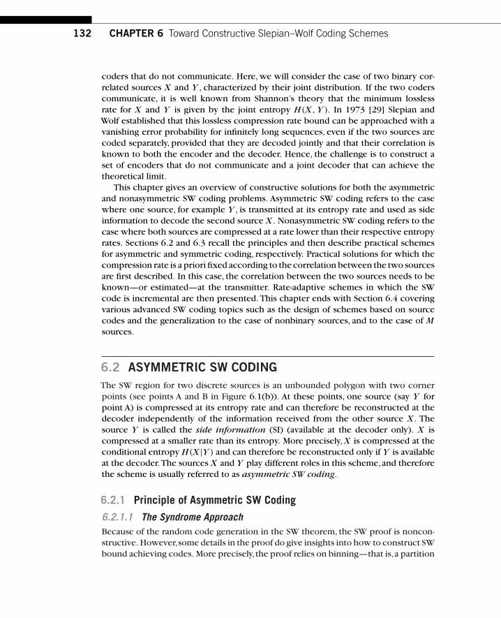
132 CHAPTER 6 Toward Constructive Slepian–Wolf Coding Schemes
coders that do not communicate. Here, we will consider the case of two binary cor-related sources X and Y , characterized by their joint distribution. If the two coderscommunicate, it is well known from Shannon’s theory that the minimum losslessrate for X and Y is given by the joint entropy H(X, Y ). In 1973 [29] Slepian andWolf established that this lossless compression rate bound can be approached with avanishing error probability for infinitely long sequences, even if the two sources arecoded separately, provided that they are decoded jointly and that their correlation isknown to both the encoder and the decoder. Hence, the challenge is to construct aset of encoders that do not communicate and a joint decoder that can achieve thetheoretical limit.
This chapter gives an overview of constructive solutions for both the asymmetricand nonasymmetric SW coding problems. Asymmetric SW coding refers to the casewhere one source, for example Y , is transmitted at its entropy rate and used as sideinformation to decode the second source X . Nonasymmetric SW coding refers to thecase where both sources are compressed at a rate lower than their respective entropyrates. Sections 6.2 and 6.3 recall the principles and then describe practical schemesfor asymmetric and symmetric coding, respectively. Practical solutions for which thecompression rate is a priori fixed according to the correlation between the two sourcesare first described. In this case, the correlation between the two sources needs to beknown—or estimated—at the transmitter. Rate-adaptive schemes in which the SWcode is incremental are then presented. This chapter ends with Section 6.4 coveringvarious advanced SW coding topics such as the design of schemes based on sourcecodes and the generalization to the case of nonbinary sources, and to the case of Msources.
6.2 ASYMMETRIC SW CODINGThe SW region for two discrete sources is an unbounded polygon with two cornerpoints (see points A and B in Figure 6.1(b)). At these points, one source (say Y forpoint A) is compressed at its entropy rate and can therefore be reconstructed at thedecoder independently of the information received from the other source X . Thesource Y is called the side information (SI) (available at the decoder only). X iscompressed at a smaller rate than its entropy. More precisely, X is compressed at theconditional entropy H(X |Y ) and can therefore be reconstructed only if Y is availableat the decoder.The sources X and Y play different roles in this scheme,and thereforethe scheme is usually referred to as asymmetric SW coding.
6.2.1 Principle of Asymmetric SW Coding
6.2.1.1 The Syndrome ApproachBecause of the random code generation in the SW theorem, the SW proof is noncon-structive. However,some details in the proof do give insights into how to construct SWbound achieving codes. More precisely,the proof relies on binning—that is,a partition
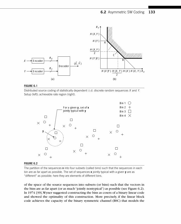
6.2 Asymmetric SW Coding 133
H (X, Y ) RX
H (Y )
RY
B
A
C
H (X |Y )
H (Y |X )
H (X, Y ) H (X )2
H (X,Y )
H (X,Y )2
(b)
Encoder
Encoder
Decoder
X
YRY
RX
(X, Y )
(a)
ˆ ˆ
FIGURE 6.1
Distributed source coding of statistically dependent i.i.d. discrete random sequences X and Y.Setup (left); achievable rate region (right).
Bin 1
y
Bin 2
Bin 3
Bin 4
For a given y, set of xjointly typical with y
FIGURE 6.2
The partition of the sequences x into four subsets (called bins) such that the sequences in eachbin are as far apart as possible. The set of sequences x jointly typical with a given y are as“different” as possible: here they are elements of different bins.
of the space of the source sequences into subsets (or bins) such that the vectors inthe bins are as far apart (or as much “jointly nontypical”) as possible (see Figure 6.2).In 1974 [39],Wyner suggested constructing the bins as cosets of a binary linear codeand showed the optimality of this construction. More precisely, if the linear blockcode achieves the capacity of the binary symmetric channel (BSC) that models the

134 CHAPTER 6 Toward Constructive Slepian–Wolf Coding Schemes
correlation between the two sources, then this capacity-achieving channel code canbe turned into a SW-achieving source code.
In order to present Wyner’s algebraic binning scheme, we first review some nota-tions on binary linear codes. A binary (n, k) code C is defined by an (n�k)�nparity-check matrix H and contains all the n-length vectors1 x such that xHT �0:
C �{x :xHT �0
}.
Notice that the code C is equivalently defined by a k�n generator matrix G such thatC �{x :x �uG}, where u is a k-bit vector.
If H has full row rank, then the rate of the channel code is k/n. Moreover, for agood code, all the vectors of the code (called words or codewords) have maximumHamming distance. The code partitions the space containing 2n sequences into 2n�k
cosets of 2k words with maximum Hamming distance. Each coset is indexed by an(n�k)-length syndrome, defined as s�xHT . In other words, all sequences in a cosetshare the same syndrome:Cs �{x :xHT �s}. Moreover,as a consequence of the linear-ity of the code, a coset results from the translation of the code by any representativeof the coset:
�v∈Cs, Cs �C⊕v. (6.1)
A geometric approach to binary coding visualizes binary sequences of length n asvertices of an n-dimensional cube. In Figure 6.3, the code C (the set of codewords orthe set of vectors of syndrome 0 that is represented with •) is a subspace of {0, 1}3,whereas the coset with syndrome 1, denoted C1 and represented with ◦, is an affinesubspace parallel to C. Notice that properties of a subspace and the linearity property(6.1) are satisfied (to verify this, all operations have to be performed over the finitefield of order 2).
If a codeword x is sent over a BSC with crossover probability p and error sequencez, the received sequence is y �x �z. Maximum likelihood (ML) decoding over theBSC searches for the closest codeword to y with respect to the Hamming distancedH (., .):
x �arg minx:x∈C
dH (x, y).
This can be implemented with syndrome decoding.This decoding relies on a functionf : {0, 1}n�k→{0, 1}n,which computes for each syndrome a representative called thecoset leader that has minimum Hamming weight.Thus,a syndrome decoder first com-putes the syndrome of the received sequence: s�yHT , then the coset leader f (s).This coset leader is the ML estimate of the error pattern z. Finally, the ML estimate ofx is given by x �y⊕ f (yHT ).
In order to use such a code for the asymmetric SW problem,Wyner [39] suggestsconstructing bins as cosets of a capacity-achieving parity check code. Let x and y
1 All vectors are line vectors, and T denotes transposition. Moreover,⊕ denotes the addition over thefinite field of order 2 and � the addition over the real field.
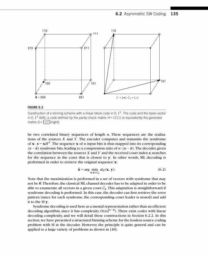
6.2 Asymmetric SW Coding 135
0010 � 000
110
100 101
111
011010
101
110
C C
FIGURE 6.3
Construction of a binning scheme with a linear block code in 0, 13. The cube and the basis vectorin 0, 13 (left); a code defined by the parity-check matrix H� (111) or equivalently the generatormatrix G =(110
101)(right).
be two correlated binary sequences of length n. These sequences are the realiza-tions of the sources X and Y . The encoder computes and transmits the syndromeof x: s�xHT . The sequence x of n input bits is thus mapped into its corresponding(n�k) syndrome bits, leading to a compression ratio of n :(n�k).The decoder,giventhe correlation between the sources X and Y and the received coset index s, searchesfor the sequence in the coset that is closest to y. In other words, ML decoding isperformed in order to retrieve the original sequence x:
x �arg minx:x∈Cs
dH (x, y). (6.2)
Note that the maximization is performed in a set of vectors with syndrome that maynot be 0.Therefore, the classical ML channel decoder has to be adapted in order to beable to enumerate all vectors in a given coset Cs. This adaptation is straightforward ifsyndrome decoding is performed. In this case, the decoder can first retrieve the errorpattern (since for each syndrome, the corresponding coset leader is stored) and addit to the SI y.
Syndrome decoding is used here as a mental representation rather than an efficientdecoding algorithm, since it has complexity O(n2n�k). There exist codes with lineardecoding complexity, and we will detail these constructions in Section 6.2.2. In thissection,we have presented a structured binning scheme for the lossless source codingproblem with SI at the decoder. However, the principle is quite general and can beapplied to a large variety of problems as shown in [40].
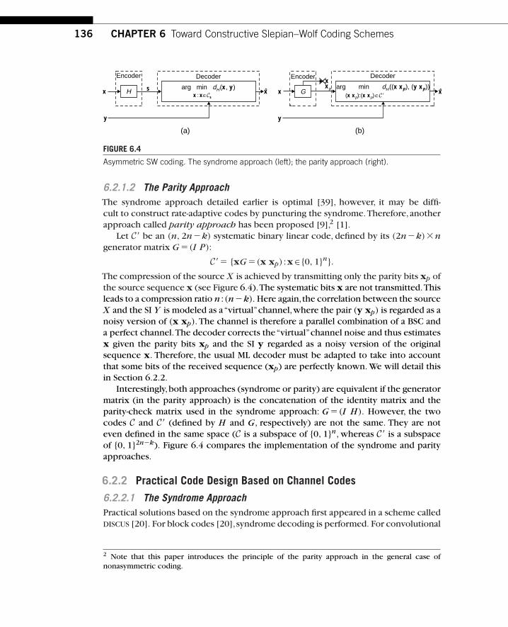
136 CHAPTER 6 Toward Constructive Slepian–Wolf Coding Schemes
(a) (b)
x
DecoderEncoder
y
s xHarg min dH (x, y)
x : x∈Cs
xpx
DecoderEncoder
y
xGarg min dH ((x xp), (y xp))
(x xp):(x xp)∈C 9
x
FIGURE 6.4
Asymmetric SW coding. The syndrome approach (left); the parity approach (right).
6.2.1.2 The Parity ApproachThe syndrome approach detailed earlier is optimal [39], however, it may be diffi-cult to construct rate-adaptive codes by puncturing the syndrome.Therefore, anotherapproach called parity approach has been proposed [9],2 [1].
Let C� be an (n, 2n�k) systematic binary linear code, defined by its (2n�k)�ngenerator matrix G �(I P):
C�� {xG �(x xp) :x∈{0, 1}n}.The compression of the source X is achieved by transmitting only the parity bits xp ofthe source sequence x (see Figure 6.4).The systematic bits x are not transmitted.Thisleads to a compression ratio n :(n�k). Here again,the correlation between the sourceX and the SI Y is modeled as a“virtual”channel,where the pair (y xp) is regarded as anoisy version of (x xp). The channel is therefore a parallel combination of a BSC anda perfect channel.The decoder corrects the“virtual”channel noise and thus estimatesx given the parity bits xp and the SI y regarded as a noisy version of the originalsequence x. Therefore, the usual ML decoder must be adapted to take into accountthat some bits of the received sequence (xp) are perfectly known. We will detail thisin Section 6.2.2.
Interestingly,both approaches (syndrome or parity) are equivalent if the generatormatrix (in the parity approach) is the concatenation of the identity matrix and theparity-check matrix used in the syndrome approach: G �(I H). However, the twocodes C and C� (defined by H and G, respectively) are not the same. They are noteven defined in the same space (C is a subspace of {0, 1}n, whereas C� is a subspaceof {0, 1}2n�k). Figure 6.4 compares the implementation of the syndrome and parityapproaches.
6.2.2 Practical Code Design Based on Channel Codes
6.2.2.1 The Syndrome ApproachPractical solutions based on the syndrome approach first appeared in a scheme calledDISCUS [20]. For block codes [20],syndrome decoding is performed. For convolutional
2 Note that this paper introduces the principle of the parity approach in the general case ofnonasymmetric coding.

6.2 Asymmetric SW Coding 137
codes, the authors in [20] propose to apply the Viterbi decoding on a modified trellis.In order to solve the problem (6.2), the decoder is modified so that it can enumerateall the codewords in a given coset. The method uses the linearity property (6.1). Forsystematic convolutional codes, a representative of the coset is the concatenation ofthe k-length zero vector and the n�k-length syndrome s. This representative is thenadded to all the codewords labeling the edges of the trellis (see Figure 6.5). Note thatthe states of the trellis depend on the information bits,and thus on the systematic bitsonly. Thus, there exists one trellis section per syndrome value. The decoder, knowingthe syndrome s,searches for the sequence with that particular syndrome that is closestto y. First, it builds the complete trellis. Each section of the trellis is determined bythe syndrome. Once the whole trellis is built, theViterbi algorithm chooses the closestsequence to the received y.
A variation of the above method is proposed in [35], where the translation bya coset representative is performed outside the decoder (see Figure 6.6). First, therepresentative (0 s) is computed (this step is called inverse syndrome former—ISF)and added to y. Then the decoding is performed (in the coset of syndrome 0), andfinally the representative is retrieved from the output of the decoder. The advantageof this method is to use a conventional Viterbi decoder without a need to modify it.This method can also be applied to turbo codes [35]. In this case, two syndromes(s1, s2) are computed, one for each constituent code. A representative of the coset is(0 s1 s2).
The authors in [24] propose a SW scheme based on convolutional codes and turbocodes that can be used for any code (not only systematic convolutional code). Ratherthan considering the usual trellis based on the generator matrix of the code, the
x1(D )
x2(D )
�2(D )�1(D )DD
x1 x2�1 �2
00
01
10
11
00
00
10
10
01
01
11
11
00
�1 �2x1 x2
1100
0011
01
10
10
01
11%(0 s)
10
01
(a) (b) s 5 0 (c) s 5 1
FIGURE 6.5
Block diagram (a) and trellises (b, c) for the systematic convolutional code H = [1 57 ].
The diagram (a) defines the states �1(D) �2(D) of the trellis, where D is a dummy variablerepresenting a time offset. The trellis section in (b) corresponds to the syndrome value s = 0 andis called the principal trellis. The complementary trellis corresponds to s = 1 and is obtained byadding (0 s) to all the codewords labeling the edges of the principal trellis.

138 CHAPTER 6 Toward Constructive Slepian–Wolf Coding Schemes
H ISF
Usual channeldecoder
x
y
s
x
Decoder
Encoder
(0 s)
FIGURE 6.6
Implementation of the syndrome approach with a usual channel decoder. ISF stands for inversesyndrome former and computes a representative of the coset with syndrome s.
D D
(a)
�1(D ) �2(D )
s (D )
x1(D )
x2(D )
x1 x2�1 �2
11
11
1010
01
01
00
00
00
01
10
11(c) s 5 1(b) s 5 0
x1x2�1�2
00
01
10
11
00
00
01
01
10
10
11
11
FIGURE 6.7
Block diagram (a) and syndrome trellises (b–c) for the rate 1/2 convolutional code H = [5 7].The states �1(D) �2(D) are defined in the block diagram (a). Two trellis sections are obtained: onefor the syndrome value s = 0 (b) and one for s = 1 (c).
decoder is based on a syndrome trellis.This trellis was first proposed for binary linearblock codes [38] and was then generalized to convolutional codes [28]. Such a trelliscan enumerate a set of sequences in any coset. More precisely, a section correspondsto the reception of n bits of x and n�k syndrome bits (see Figure 6.7). Thus, thereexist 2n�k possible trellis sections, one for each syndrome value. The decoder, know-ing the syndrome s, searches for the sequence with that particular syndrome that isclosest to y. First,it builds the complete trellis. Each section of the trellis is determinedby the syndrome. Once the whole trellis is built, the Viterbi algorithm is performedand chooses the closest sequence to the received y.
For low-density parity-check (LDPC) codes, the belief propagation decoder can beadapted to take into account the syndrome [16]. More precisely, the syndrome bitsare added to the graph such that each syndrome bit is connected to the parity check
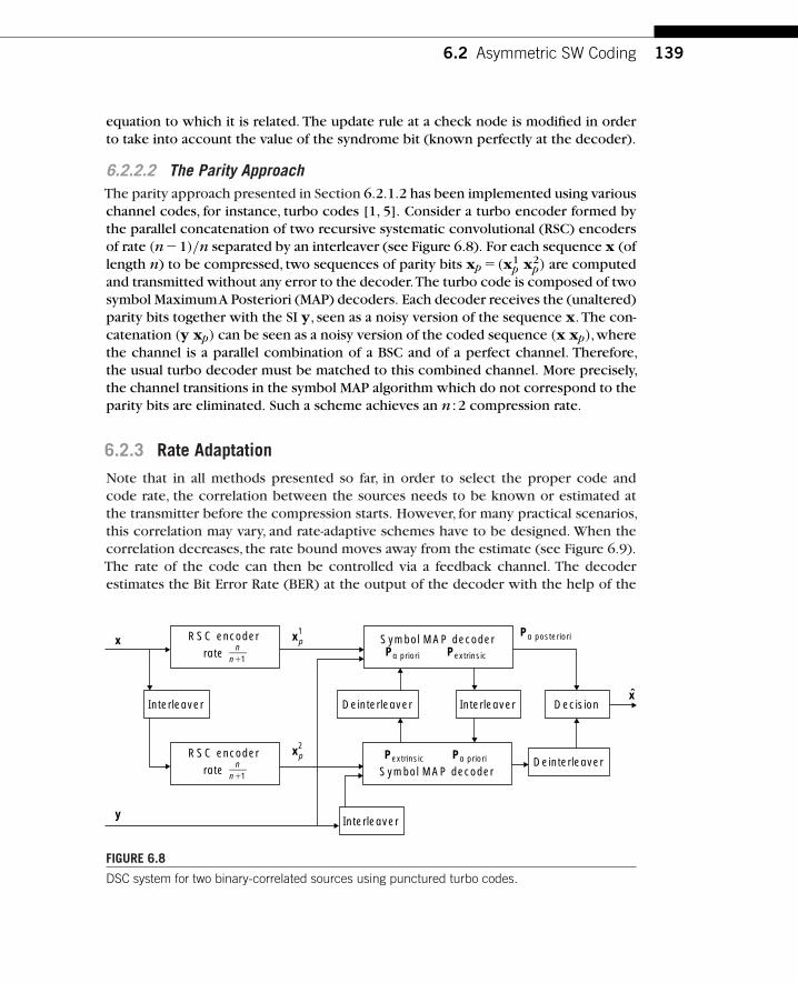
6.2 Asymmetric SW Coding 139
equation to which it is related. The update rule at a check node is modified in orderto take into account the value of the syndrome bit (known perfectly at the decoder).
6.2.2.2 The Parity ApproachThe parity approach presented in Section 6.2.1.2 has been implemented using variouschannel codes, for instance, turbo codes [1, 5]. Consider a turbo encoder formed bythe parallel concatenation of two recursive systematic convolutional (RSC) encodersof rate (n�1)/n separated by an interleaver (see Figure 6.8). For each sequence x (oflength n) to be compressed, two sequences of parity bits xp �(x1
p x2p) are computed
and transmitted without any error to the decoder.The turbo code is composed of twosymbol MaximumA Posteriori (MAP) decoders. Each decoder receives the (unaltered)parity bits together with the SI y, seen as a noisy version of the sequence x. The con-catenation (y xp) can be seen as a noisy version of the coded sequence (x xp),wherethe channel is a parallel combination of a BSC and of a perfect channel. Therefore,the usual turbo decoder must be matched to this combined channel. More precisely,the channel transitions in the symbol MAP algorithm which do not correspond to theparity bits are eliminated. Such a scheme achieves an n :2 compression rate.
6.2.3 Rate Adaptation
Note that in all methods presented so far, in order to select the proper code andcode rate, the correlation between the sources needs to be known or estimated atthe transmitter before the compression starts. However, for many practical scenarios,this correlation may vary, and rate-adaptive schemes have to be designed. When thecorrelation decreases, the rate bound moves away from the estimate (see Figure 6.9).The rate of the code can then be controlled via a feedback channel. The decoderestimates the Bit Error Rate (BER) at the output of the decoder with the help of the
Pa priori Pextrinsic
Symbol MAP decoder
InterleaverDeinterleaver
RSC encoderrate n
n11
RSC encoderrate n
n11
Interleaver Decision
Deinterleaver
Interleaver
Pa posteriorix
y
x2p
x1p
x
Pa prioriPextrinsic
Symbol MAP decoder
FIGURE 6.8
DSC system for two binary-correlated sources using punctured turbo codes.

140 CHAPTER 6 Toward Constructive Slepian–Wolf Coding Schemes
log-likelihood ratios computed by the channel decoder. If the BER at the output ofthe decoder exceeds a given value, more bits are requested from the encoder. In thiscontext of feedback-controlled schemes, the code should be incremental such thatthe encoder does not need to re-encode the data.The first bits are kept,and additionalbits are only sent upon request. In the following, we present various rate-adaptivemethods and specify whether or not they are incremental.
6.2.3.1 The Parity ApproachThe parity approach was originally proposed to easily construct rate-adaptive schemes(see Section 6.2.2). At the encoder, the parity bits are punctured (some parity bitsare not transmitted), and the decoder compensates for this puncturing, using stan-dard techniques coming from channel coding. The source sequence x is compressedthrough some punctured parity bits xp, and the decoder retrieves the originalsequence aided by the SI y. The sequence (y xp) can be seen as the output of achannel, which is a combination of a perfect channel (unpunctured parity bits), anerasure channel (punctured parity bits), and a BSC channel (correlation between thesources x and y). The method is by construction incremental.
6.2.3.2 The Syndrome ApproachBecause of the optimality of the syndrome approach [39], a natural design of a rate-adaptive scheme consists of puncturing the syndrome. However, using puncturingmechanisms leads to performance degradation as reported in [15, 32, 36]. More pre-cisely, it is shown in [32] that the syndrome approach is very sensitive to errors
B
H (X ) RX
H (Y )
RY
A
Slepian–Wolf bound for a given correlation
FIGURE 6.9
Evolution of the SW region, when the correlation between the sources varies.

6.2 Asymmetric SW Coding 141
or erasures, which indicates that the puncturing of syndromes will lead to perfor-mance degradation. Therefore, the first contributions avoid or compensate for thisperformance degradation.
A first method proposed in [15] punctures the parity bits rather than the syndromebits. Each puncturing pattern defines a new code for which a parity check matrixcan be computed. Then, one can construct a syndrome former and inverse syndromeformer for the new punctured code (presented in Section 6.2.1.2).This method can beimplemented using any code, in particular convolutional and turbo codes. However,the resulting code is not incremental.
A first incremental SW coding scheme based on Serially Concatenated Accumulate(SCA) codes is proposed in [7].An inner encoder concatenates the first source bit withthe modulo-2 sum of consecutive pairs of source bits. The output of the accumulatoris interleaved and fed into a so-called base code,which is either an extended Hammingcode or a product of single-parity check codes, which then compute the syndromebits. The accumulator code is of rate 1, so that the compression rate is controlledby the base code. The base code is first decoded using a MAP decoder for extendedHamming codes or a belief propagation algorithm for product parity-check codes.The accumulator code is decoded with a symbol MAP decoder, A turbo-like algorithmiterates between both decoders.
The authors in [36] investigate the puncturing of LDPC (low-density parity-checkcode) encoded syndromes.To avoid degrading the performance of the LDPC code,thesyndrome bits are first protected with an accumulator code before being punctured.Here also the accumulator code is of rate 1, so that the compression rate is not modi-fied.The combined effect of the puncturing and of the accumulator code is equivalentto merging some rows of the parity-check matrix by adding them. This defines a setof parity-check matrices, one for each rate. Then, for each parity-check matrix, decod-ing is performed according to the modified sum-product algorithm [16] presented inSection 6.2.1.1. An interesting feature of this method is that it is incremental. If themerging of rows satisfies a regularity rule (one can only add two rows that have no“1” at the same column position), then the accumulated syndrome value of the new(smallest compression rate) matrix can be computed by adding the previous syndromevalue (corresponding to the highest compression rate matrix) to the current one.Theperformance of the method is shown in Figure 6.10(a). Another method is proposedin [14]. Instead of protecting the syndrome bits, the authors combine the syndromeand the parity approaches. Given an input vector x of length n, the encoder transmitsm syndrome bits plus l parity bits, defining an (n� l, n�m) linear error-correctingcode. Rate adaptation is then performed by puncturing the parity bits.
In [24],the optimal decoder for convolutional codes under syndrome puncturing isdesigned. It is shown that performance degradation due to syndrome puncturing canbe avoided without a need to encode (or protect) the syndromes.When syndrome bitsare punctured,the optimal decoder should in principle search for the closest sequencein a union of cosets. This union corresponds to all possible syndromes that equal thereceived syndrome in the unpunctured positions. Therefore, the number of cosetsgrows exponentially with the number of punctured bits.A brute force decoder consists
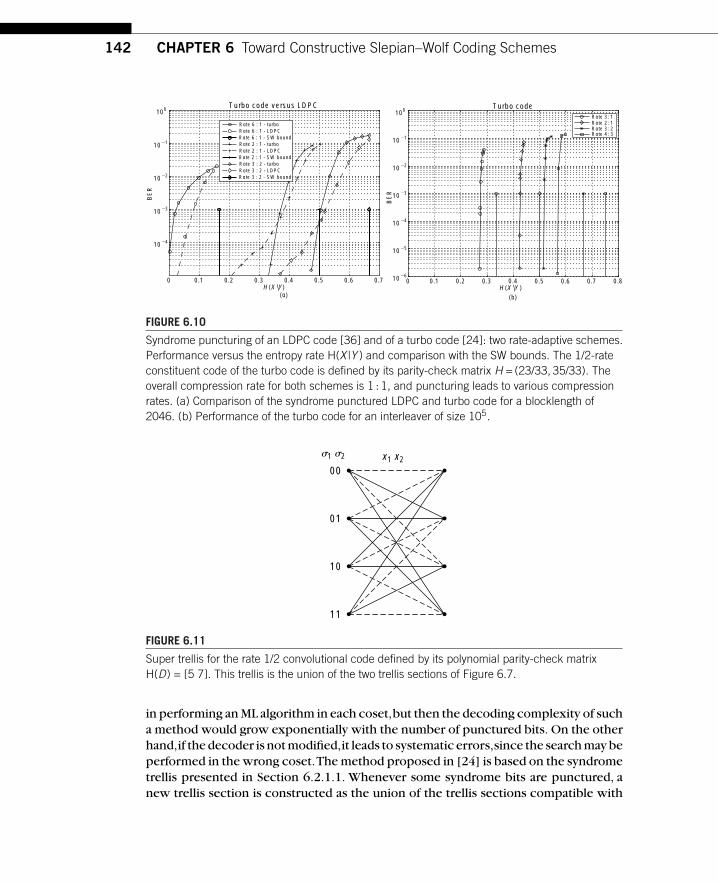
142 CHAPTER 6 Toward Constructive Slepian–Wolf Coding Schemes
0 0.1 0.2 0.3 0.4 0.5 0.6 0.7
1024
1023
1022
1021
100
H (X |Y)
BE
R
Turbo code versus LDPC
Rate 6 : 1 - turboRate 6 : 1 - LDPCRate 6 : 1 - SW boundRate 2 : 1 - turboRate 2 : 1 - LDPCRate 2 : 1 - SW boundRate 3 : 2 - turboRate 3 : 2 - LDPCRate 3 : 2 - SW bound
(a)
0 0.1 0.2 0.3 0.4 0.5 0.6 0.7 0.8H (X |Y )
BE
R
Turbo code
(b)
1024
1025
1026
1023
1022
1021
100Rate 3 : 1Rate 2 : 1Rate 3 : 2Rate 4 : 3
FIGURE 6.10
Syndrome puncturing of an LDPC code [36] and of a turbo code [24]: two rate-adaptive schemes.Performance versus the entropy rate H(X |Y ) and comparison with the SW bounds. The 1/2-rateconstituent code of the turbo code is defined by its parity-check matrix H = (23/33, 35/33). Theoverall compression rate for both schemes is 1 : 1, and puncturing leads to various compressionrates. (a) Comparison of the syndrome punctured LDPC and turbo code for a blocklength of2046. (b) Performance of the turbo code for an interleaver of size 105.
00
�1 �2 x1 x2
11
10
01
FIGURE 6.11
Super trellis for the rate 1/2 convolutional code defined by its polynomial parity-check matrixH(D) = [5 7]. This trellis is the union of the two trellis sections of Figure 6.7.
in performing an ML algorithm in each coset,but then the decoding complexity of sucha method would grow exponentially with the number of punctured bits. On the otherhand,if the decoder is not modified,it leads to systematic errors,since the search may beperformed in the wrong coset.The method proposed in [24] is based on the syndrometrellis presented in Section 6.2.1.1. Whenever some syndrome bits are punctured, anew trellis section is constructed as the union of the trellis sections compatible with
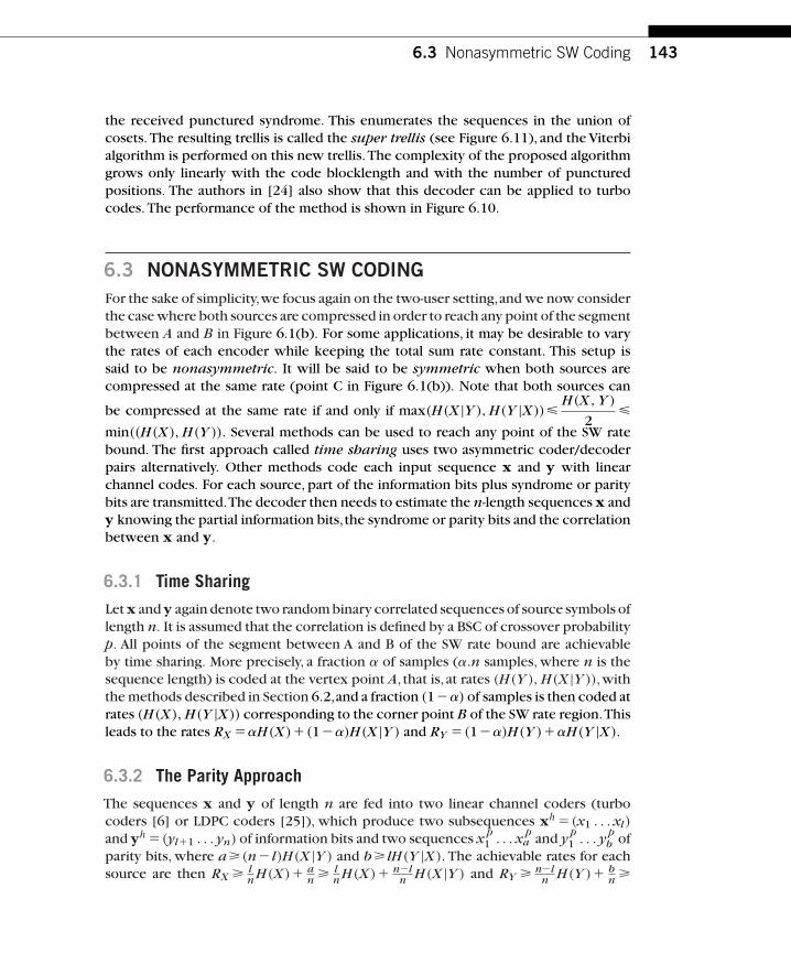
6.3 Nonasymmetric SW Coding 143
the received punctured syndrome. This enumerates the sequences in the union ofcosets. The resulting trellis is called the super trellis (see Figure 6.11), and the Viterbialgorithm is performed on this new trellis.The complexity of the proposed algorithmgrows only linearly with the code blocklength and with the number of puncturedpositions. The authors in [24] also show that this decoder can be applied to turbocodes. The performance of the method is shown in Figure 6.10.
6.3 NONASYMMETRIC SW CODINGFor the sake of simplicity,we focus again on the two-user setting,and we now considerthe case where both sources are compressed in order to reach any point of the segmentbetween A and B in Figure 6.1(b). For some applications, it may be desirable to varythe rates of each encoder while keeping the total sum rate constant. This setup issaid to be nonasymmetric. It will be said to be symmetric when both sources arecompressed at the same rate (point C in Figure 6.1(b)). Note that both sources can
be compressed at the same rate if and only if max(H(X |Y ), H(Y |X))�H(X, Y )
2�
min((H(X), H(Y )). Several methods can be used to reach any point of the SW ratebound. The first approach called time sharing uses two asymmetric coder/decoderpairs alternatively. Other methods code each input sequence x and y with linearchannel codes. For each source, part of the information bits plus syndrome or paritybits are transmitted.The decoder then needs to estimate the n-length sequences x andy knowing the partial information bits,the syndrome or parity bits and the correlationbetween x and y.
6.3.1 Time Sharing
Let x and y again denote two random binary correlated sequences of source symbols oflength n. It is assumed that the correlation is defined by a BSC of crossover probabilityp. All points of the segment between A and B of the SW rate bound are achievableby time sharing. More precisely, a fraction � of samples (�.n samples, where n is thesequence length) is coded at the vertex point A, that is, at rates (H(Y ), H(X |Y )),withthe methods described in Section 6.2,and a fraction (1��) of samples is then coded atrates (H(X), H(Y |X)) corresponding to the corner point B of the SW rate region.Thisleads to the rates RX ��H(X)�(1��)H(X |Y ) and RY �(1��)H(Y )��H(Y |X).
6.3.2 The Parity Approach
The sequences x and y of length n are fed into two linear channel coders (turbocoders [6] or LDPC coders [25]), which produce two subsequences xh �(x1 . . . xl)
and yh �(yl�1 . . . yn) of information bits and two sequences x p1 . . . x p
a and y p1 . . . y p
b ofparity bits, where a(n� l)H(X |Y ) and b lH(Y |X). The achievable rates for eachsource are then RX l
nH(X)� an l
nH(X)� n�ln H(X |Y ) and RY n�l
n H(Y )� bn

144 CHAPTER 6 Toward Constructive Slepian–Wolf Coding Schemes
n�ln H(Y )� l
nH(Y |X). The SW boundary can be approached by varying the ratio ln
between 0 and 1. Unlike the time-sharing approach, the parity bits are computed onthe entire input sequences of length n. The sequence (xhxp) is regarded as a noisyversion of the sequence (ypyh). As in the asymmetric setup, the channel is a parallelcombination of a BSC and of a perfect channel.The decoder then needs to estimate xand y given (xhxp) and (ypyh).
A first practical implementation of the parity approach is proposed in [9] with turbocodes and considers the particular case of symmetric SW coding.The solution is thenextended to reach any point of the SW boundary in [6, 8]. In [8], the two informationsequences of length n are encoded with a systematic punctured turbo code. Theinformation bits of the second source are interleaved before being fed to the encoder.All the systematic bits as well as a subset of the parity bits are punctured in order toleave only a bits for the sequence x and b bits for the sequence y. Each turbo decoderproceeds in the standard way, with the difference that part of the bits is received viaan ideal channel. After each iteration, the measures obtained as a result of a turbodecoding on each input bit of one sequence, for example, x, are passed as additionalextrinsic information to the turbo decoder used to estimate the sequence y, via thebinary symmetric correlation channel (i.e., P(yk �0)�(1�p)P(xk �0)�pP(xk �1)).
Another implementation of the parity approach is described in [25] with LDPCcodes and later studied in [26] for short to moderate-length codes.The decoder needsto determine an n-length sequence from the part of information bits and parity bitsreceived for the sequence x and from the correlated sequence y. For this, a message-passing algorithm is used by setting the LLR (log-likelihood ratio) of the bits receivedvia the ideal channel to infinity.The LLR of the bits received via the correlation channelare set to log(
1�pp ).The LLR for the punctured bits are set to zero.Two sets of degree
distributions for the variables nodes are used to account for the fact that informationbits are received via the correlation channel, whereas the parity bits are received viaan ideal channel.
6.3.3 The Syndrome Approach
Let us consider an (n, k) linear channel code C defined by its generator matrix Gk�n
and its parity-check matrix H(n�k)�n.A syndrome approach was first proposed in [19],based on the construction of two independent linear binary codes C1 and C2 with G1
and G2 as generator matrices, obtained from the main code C. More precisely, thegenerator matrices G1 and G2 of the two subcodes are formed by extracting m1 andm2 lines,respectively,where m1 �m2 �k,from the matrix G of the code C.The parity-check matrices H1 and H2 are then of size (n�m1)�n and (n�m2)�n,respectively.A geometric interpretation of the code splitting is shown in Figure 6.12. Each codersends a syndrome,defined as sx �xHT
1 and sy �yHT2 ,respectively, to index the cosets
of C1 and C2 containing x and y. The total rate for encoding the input sequencesof length n is then n�m1 �n�m2 �2n�k bits. The cosets containing x and y aretranslated versions of the codes C1 and C2 (i.e., the cosets having null syndromes)

6.3 Nonasymmetric SW Coding 145
001
110
100 101
111
011010
000001
110
100101
111
011010
000
C101 5 {·}
C1 5 {·}
C110 5 { }
C111 5 { }
C101 5 {·}C2 5 {·}
C210 5 { }
C211 5 { }
FIGURE 6.12
Splitting the code of Figure 6.3 into two subcodes: code C1 defined by G1 = (110) or H1 = (110001)
(left); code C2 defined by G2 = (101) or H2 = (010101)(right).
by vectors tx and ty. This translation is illustrated in Figure 6.12, where the additionby the translation vector is performed over the finite field {0, 1}. The codes C1 andC2 must be chosen such that all pairs (x, y) can be determined uniquely given thetwo coset indexes. We now explain how to determine a pair (x, y) from a usual MLdecoder.
Let uxG1 and uyG2 define codewords in C1 and C2. By definition these vectorshave a null syndrome.All possible codewords in a coset of syndrome s can be enumer-ated by translating a codeword belonging to the coset of null syndrome by a vector tbelonging to the coset of syndrome s (see Equation (6.1)). If the code is systematic,a candidate for the translating vector is t �(0 s), as explained in Section 6.2.2. Thus,x and y can be seen as translated versions of codewords belonging to the cosets ofnull syndrome of the codes C1 and C2, respectively. The vectors x and y can thus beexpressed as x �uxG1⊕(0 sx), y �uyG2⊕(0 sy), where tx �(0 sx) and ty �(0 sy)
are the representatives of the cosets of C1 and C2 with syndromes sx and sy. Thedecoder must search for a pair of codewords, one from each translated coset of C1
and C2. When receiving the syndromes sx and sy, it first finds a codeword c of themain code C (which is actually the error pattern between x and y) that is closest tothe vector t � tx⊕ ty �(0 sx)⊕(0 sy).The error pattern x⊕y is the minimum-weightcodeword having the same syndrome as the vector t. If the code is systematic, thesequences x and y are reconstructed as x � uxG1⊕ tx and y � uyG2⊕ ty, where ux
and uy are the systematic bits of the codeword c. This method achieves the optimalSW compression sum rate if the global code C achieves the capacity of the equiv-alent correlation channel (between x and y). The number of lines assigned to G1
(and therefore to G2) allows choosing any rate on the dominant face of the SW

146 CHAPTER 6 Toward Constructive Slepian–Wolf Coding Schemes
region (between points A and B in Figure 6.1(b)). The above ideas are further devel-oped in [30, 31], for nonsystematic linear codes. The code construction has beenextended in [27] to the case where the sources X and Y are binary but nonuniformlydistributed.
In a second approach proposed in [10], the vectors x and y belong to the samecoset of a unique code C,which is the translated version of the coset of null syndromeby a vector t. Each source vector is identified by a syndrome computed with theparity-check matrix H of the code C plus part of the source information bits [10].The syndromes sT
x �HxT and sTy �HyT , of length (n�k), are thus computed for
both sequences and transmitted to the decoder. In addition, the k� first bits of x(denoted xk�
1 ) and the k�k� next bits for the source y (denoted ykk��1) are transmitted
as systematic bits, where k� is an integer so that k�∈[0, k]. The total rate for thesequences x and y of length n is, respectively,n�k�k� and n�k� bits.The structureof the coders is depicted in Figure 6.13. Note that k��k and k��0 correspond tothe two asymmetric setups with rates given by the corner points A and B of the SWregion.
As in the asymmetric case,the representative of the coset is thus the concatenationof the transmitted information bits (k� bits for the sequence x) and of the (n�k)-lengthsyndrome vector. As in the first approach, when receiving the syndromes sx and sy,the decoder must find a codeword c of the code C that is closest to the translatingvector t � tx⊕ ty �(0 sx)⊕(0 sy). For this, it first computes sz �sx⊕sy, which is thesyndrome of the error pattern z between x and y (z�x⊕y). In [10], a modifiedLDPC decoder estimates z� x⊕y from the syndrome sz and the all-zero word of sizen (see Figure 6.14) [16]. The error pattern z is the smallest weight codeword withsyndrome sz . When convolutional and turbo codes are used, the estimation of theerror pattern can be performed with a conventional Viterbi decoder and an inversesyndrome former (ISF) [33] or with a syndrome decoder [24] (see Section 6.2.2 forfurther details).
ykk9+1
H
nEncoder X
k9
n 2 ksx
xk19
Hyn1
xn1
nEncoder Y
k 2 k9
n 2 ksy
FIGURE 6.13
The nonasymmetric coders in the syndrome approach [10]. A single code C (determined by theparity check matrix H) is used for each sequence to be compressed.

6.3 Nonasymmetric SW Coding 147
nb0
n 2 k
Decoder
a:a∈Cs
n 2 k
sx
sy
s
â z
B21 (sx Å A xk1)
x1k 9 xk
k11
zkk911 Å yk
k911
za = arg min dH (a, b)ˆ
xkn
11
y1k 9 yk
k911 yk
n11
1.
2.
sx
FIGURE 6.14
Nonasymmetric decoder: estimation of the error pattern z�x⊕y (left); reconstruction of thesource sequence x (right).
Once the error pattern is found, the subsequences of information bits xkk��1 and
yk�1 can be retrieved from the error pattern z�x⊕y as (see Figure 6.14–right)
xkk��1 �yk
k��1⊕ zkk��1 and yk�
1 �xk�1 ⊕ zk�
1 . (6.3)
Subsequences of n�k bits (i.e., xnk�1 and yn
k�1), remain to be computed for bothsequences. Let us assume that H �(A B), where B is an invertible square matrix ofdimension (n�k)�(n�k). Note that for a rate k/n channel code, the parity-checkmatrix H has rank n�k. Therefore, one can always find a permutation to be appliedon the columns of H so that the resulting parity-check matrix has the right form.Thus,sx �Hx �(A B)x �A xk
1⊕B xnk�1,and the remaining n�k unknown bits of the
sequence x (and similarly for the sequence y) can be computed as
xnk�1 �B�1 (sx⊕A xk
1), (6.4)
where B�1 denotes the inverse of the matrix B [10]. The authors in [10] have usedLDPC codes.
If the error pattern is not perfectly estimated, the estimation of the remainingsymbols xn
k�1 in Equation (6.4) may yield error propagation. Note that the unknownpositions in the vector x are design parameters. These positions (or, equivalently, thecolumns of the matrix H to be extracted in order to build the matrix B) can be chosenso that the inverse B�1 is as sparse as possible. Figure 6.15 shows the BER of the errorpattern z (continuous line) and its effect on the estimation of the source sequencex. Performance is shown for a convolutional code. The dotted curve represents theBER,when Equation (6.4) is performed with an arbitrary invertible matrix B.This BER

148 CHAPTER 6 Toward Constructive Slepian–Wolf Coding Schemes
100
0.05 0.1 0.15 0.2 0.25 0.3 0.35 0.4 0.45 0.5
BE
R
X
1021
1022
1023
1024
X - Arbitrary matrix B
X - Sparse B21
X - BCJRZSW bound
H (X Y )
FIGURE 6.15
Error propagation in the estimation of the source X. The convolutional code is defined by itsparity-check matrix H =(11 15 06
15 12 17)and is punctured over a period of four trellis sections in order toget a 2 : 1 compression rate for the source.
can be lowered to the dashed curve, if a matrix B with sparse inverse is chosen. Thislimits the error propagation. Finally, the error propagation can be further reduced, ifone applies a modified decoder to solve Equation (6.4). This decoder (Viterbi for aconvolutional code) is matched to a channel which combines a perfect channel (forxk�
1 ), a BSC (for xkk��1 with crossover probability the BER of z) and an erasure channel
(for xnk�1). Interestingly, with this decoder the BER of x remains almost the same as
that of z.
6.3.4 Source Splitting
Source splitting [21] is another approach to vary the rates between the two encoders.The approach is asymptotic and involves splitting the source into subsources having a
6.3 Nonasymmetric SW Coding 149
lower entropy. More precisely,it transforms the two source problem into a three sourceproblem where one source, for example, X is split into two i.i.d. discrete sources Uand V as U �XT and V �Y (1�T ). T is an i.i.d. binary source (which can be seen asa time-sharing sequence). By varying P(T �1), one can vary H(Y |U ) between H(Y )
and H(Y |X).The sum rate becomes RX �RY �RU �RV �RY �H(U |T )�H(Y |U )�H(V |U , Y ).A random coding argument is used to show that the rate triple is achievable[21]; however, no constructive codes are proposed.
6.3.5 Rate Adaptation
In practical applications, the correlation between the two sources may not be knownat the time of code design. It may thus be necessary, as in the asymmetric setup,to have solutions allowing for flexible rate adaptation to any correlation betweenthe two sources. Nonasymmetric rate-adaptive SW coding/decoding schemes aredirect extensions of their asymmetric counterparts. Rate adaptation is performed bysimply puncturing information, parity, or syndrome bits in the schemes describedabove.
In the parity approach, we have seen that for two correlated sequences of lengthn, the rate allocation between the two sequences is controlled by the number l ofinformation bits transmitted for each. The change in the rate allocation between thetwo sources is thus performed by puncturing more or less information bits. For a givenrate share between the two sources, rate adaptation to varying correlation is achievedby simply puncturing the parity bits. Standard decoding of punctured channel codescan then be applied.
For the syndrome approaches, as explained in Section 6.2.3, the application ofthe puncturing is less straightforward. Puncturing the syndrome bits may degradethe performance of the code. The approach considered in [34], similarly to [36] forthe asymmetric setup,consists of first protecting the syndromes with an accumulatorcode. The effect of the accumulator code followed by the puncturing is equivalent tomerging some rows of the parity-check matrix H by adding them, thus constructing amatrix Hi of dimension (n�ki)�n,of rank n�ki . In the matrix Hi ,with appropriatepermutation, one may exhibit a submatrix Bi of dimension (n�ki)�(n�ki), whichis invertible (see Equation (6.4)).The positions of the k� (k�∈[0, ki]) and ki �k� infor-mation bits transmitted for the sequences x and y, respectively, must then be chosenso that they correspond to the positions of the remaining nonfree ki columns of Hi . Ifthe correlation is not known to the encoder, the rate may be controlled via a feedbackchannel. In this case,once the error pattern z has been estimated,the decoder verifiesif the condition z HI �sz is satisfied. If this condition is not satisfied, it then requestsfor more syndrome bits. Note that, if the error pattern is not perfectly estimated, thelast step of the decoding algorithm represented by Equation (6.4) may yield error prop-agation. The coding and decoding structures are depicted in Figure 6.16. Figure 6.17illustrates the rate points achieved with a nonsymmetric SW coding/decoding schemebased on LDPC codes.

150 CHAPTER 6 Toward Constructive Slepian–Wolf Coding Schemes
Punct
Encoder Y
Encoder X
H
PunctHx1n
y1n
n
n
z
s
b0n
Feedback
Feedback
ki 2k 9
n 2ki
n 2ki
sy
sx k 9
x1k 9
ykik911
Decoder a 5 arg min dH (a, b)
a
a:a∈Cs
FIGURE 6.16
Rate-adaptive coding/decoding scheme.
0 0.2 0.4 0.6 0.8 10
0.1
0.2
0.3
0.4
0.5
0.6
0.7
0.8
0.9
1
RY (
bits
/sou
rce
sym
bol)
RX (bits/source symbol)
p 5 0.01, gap 5 0.0562 bits
p 5 0.01, theoretical bound
p 5 0.05, gap 5 0.0907 bits
p 5 0.05, theoretical bound
p 5 0.13, gap 5 0.0687 bits
p 5 0.13, theoretical bound
FIGURE 6.17
Rate points achieved for different parameters p of the binary symmetric correlation channel.
6.4 Advanced Topics 151
6.4 ADVANCED TOPICS
6.4.1 Practical Code Design Based on Source Codes
6.4.1.1 Code Design Based on Source Alphabet PartitioningThe use of source codes for SW coding was first been explored in [2] consideringHuffman codes. The approach relies on partitioning the source alphabet into groupsof symbols. One source Y is coded with a Huffman code designed according to itsstationary probability P(Y ). The alphabet of the second source X is partitioned sothat two symbols xi and xj are not grouped together if there exists a symbol y suchthat P(xi, y)�0 and P(xj, y)�0. The joint probability mass function of (X, Y ) mayneed to be slightly modified,for example,by thresholding the smallest values and thenrenormalizing, so that this condition is verified. In addition, the entropy of the groupindex must be minimum and approach at best H(X |Y ). Knowing the SI symbol yand the group index, the decoder can find the transmitted symbol x. The above codedesign based on alphabet partitioning has been formalized and generalized in [41] forarbitrary p.m.f. P(X, Y ), assuming memoryless sources. The partition can be codedwith a Huffman or an arithmetic code.
6.4.1.2 Punctured and Overlapped Arithmetic CodesDifferent solutions based on overlapped arithmetic [11] and quasi-arithmetic (QA) [3]codes, as well as punctured (quasi-)arithmetic codes [17] have appeared recently forthe case of binary sources. Arithmetic coding recursively divides the interval [0, 1)
according to the source probabilities. Let us consider a binary memoryless sourcewith probabilities denoted P0 and P1. At each symbol clock instant n, the currentinterval [Ln, Hn) is divided into two subintervals whose widths are proportional to P0
and P1 �1�P0, respectively. One of these subintervals is selected according to thevalue of the next symbol and becomes the current interval. Once the last symbol isencoded, the encoder produces a sequence of bits identifying the final subinterval.Practical implementations of arithmetic coding were first introduced in [18–22], andfurther developed in [23, 37].
The encoding and decoding processes can be modeled as state machines. Butwith optimal arithmetic coding,the number of states can grow exponentially with thesequence length. Controlled approximations can reduce the number of possible stateswithout significantly degrading compression performances [13].This fast,but reducedprecision,implementation of arithmetic coding is called quasi-arithmetic coding [13].Instead of using the real interval [0, 1], quasi-arithmetic coding is performed on aninteger interval [0, T ]. The value of T controls the trade-off between complexity, thenumber of states, and compression efficiency.
The average code length achieved per input source symbol is very close to thesource entropy. To further reduce the rate down to the conditional entropy oftwo correlated sources, two strategies can be considered: puncturing the sequenceof encoded bits [17] or overlapping the symbol probability intervals of the

152 CHAPTER 6 Toward Constructive Slepian–Wolf Coding Schemes
arithmetic [11] or quasi-arithmetic coder [3]. For the overlapped (quasi-)arithmeticcodes, at a given instant n, the probability interval [Ln, Hn) is partitioned into twosubintervals [Ln, P0(Hn �Ln)��T /2) associated with the symbol 0 and [P0(Hn �Ln)��T /2, Hn) associated with the symbol 1. The parameter � controls the over-lap between the subintervals. The larger the overlap, the lower the bit rate but thehigher the uncertainty on the decoded sequence. In both cases,overlapped and punc-tured codes, the resulting code is no longer uniquely decodable. The ambiguity onthe encoded sequence of symbols can be removed with the help of the SI (correlatedsource) and of a symbol MAP decoder.
To explain the decoding algorithm, let us first consider the punctured solution. Letx and y be two correlated sequences of length L(x). The sequence x is coded witha QA code producing a sequence of bits u of length L(u), which is then punctured.Given the received QA coded bitstream uL(u)
1 and the correlated sequence yL(x)1 (SI),
the symbol posterior marginals P(Xn �xn |uL(u)1 , yL(x)
1 ) are computed by running aBCJR algorithm [4] on the state model of the QA automaton. To cope with the factthat the QA automaton contains transitions corresponding to a varying number ofsymbols and a varying number of bits,the state model used in the decoding must keeptrack of the number of symbols being coded at a particular bit clock instant k. It ishence defined by the pairs of random variables Vk �(Nk, Mk), where Nk denotesthe state of the QA automaton and Mk represents the symbol clock value at thebit clock instant k [12]. Since the variable Mk corresponds to the symbol clock, itaccounts for the correlation between the encoded sequence and the SI.The transitionprobabilities on the state model Vk �(Nk, Mk) are equal to the transition probabil-ities between states Nk of the QA automaton, if the numbers of bits and symbolsassociated with this transition match the one defined by the automaton. The transi-tion probabilities are equal to zero otherwise.The probabilities of transition betweenstates Nk of the QA automaton depend on the source statistics and can account forsource memory. Thus, for each state � �(n, m), the BCJR algorithm computes theprobabilities �k(�)�P(Vk ��;Uk
1 ) and �k(�)�P(UL(U)k�1 |Vk ��). The branch metric
�k(��|�) used for the transition � between two states � �(n, m) and ���(n�, m�) isgiven by �k(��|�)�P(��|�)�P(b�)�P(x� |y�), where b� and x� denote the subse-quences of bits and symbols associated with given transition � on the QA automaton.The probability P(b�) is computed considering a probability of 0.5 for the punc-tured positions. The term P(x� |y�) represents the correlation channel betweenX and Y .
The decoding for the overlapped quasi-arithmetic codes proceeds in the samemanner as for the punctured solution. The only difference is in the automaton, whichin the case of overlapped codes depends not only on the distribution of the source Xbut also on the overlap factor � (for details see [17] and [3]). A second difference isin the branch metric �k(��|�) in which the term P(b�) disappears, since, in this case,all the coded bits are known to the decoder (and not punctured as in the previousmethod).
6.5 Conclusions 153
6.4.2 Generalization to Nonbinary Sources
Thus so far, we have considered only binary correlated sources. Practical applicationsoften involve nonbinary (e.g., q-ary) sources. In practice, before being encoded, theq-ary sources are first binarized. Each resulting sequence of bits is then fed to the SWcoder. For example, this is the case in [42] where the authors describe the principleusing turbo codes to compress both sources X and Y . For each source, the sequencesof bits at the output of the “symbol-to-bit” converter are interleaved and input to apunctured turbo coder.The turbo decoders act at a bit level in a standard fashion,butinformation exchange is performed between the two turbo decoders at the symbollevel.The a posteriori probabilities computed by a turbo decoder for each input bit areconverted into a measure on the corresponding q-ary symbol. The resulting symbolprobabilities are then multiplied by the conditional probabilities characterizing thecorrelation channel and fed into the second turbo decoder as extrinsic information.
6.4.3 Generalization to M Sources
The asymmetric and nonasymmetric coding schemes presented earlier can beextended to more than two sources. The practical code design approach proposedin [19] has been extended in [30] and [31] for M sources (see Section 6.3.3). Eachsubcode is constructed by selecting a subset of rows from the generator matrix Gof the starting code C. Examples of design are given for irregular repeat-accumulate(IRA) codes. However, the method is shown to be suboptimal when the number ofsources is greater (or equal) than three.The parity approach described in [25] has alsobeen extended to M sources in [26]. The sequences xi, i �1, . . . M , of length n arefed into M LDPC coders, which produce subsequences of ai �k information bits and(1�ai)�k parity bits. Joint decoding of the M sources is then performed.
6.5 CONCLUSIONSThis chapter has explained how near-capacity achieving channel codes can be usedto approach the SW rate bound. Although the problem is posed as a communicationproblem, classical channel decoders need to be modified. This chapter has outlinedthe different ways to adapt channel decoding algorithms to the Slepian–Wolf decod-ing problem. In the approaches presented, it is assumed that syndrome or parity bitsare transmitted over a perfect channel. As explained, the equivalent communicationchannel is thus the parallel combination of a BSC and a perfect channel. In some appli-cations, this may not be the case: syndrome or parity bits may have to be transmittedon an erroneous communication channel. Distributed joint source-channel codingschemes, in which the SW code acts as a single code for both source coding and chan-nel error correction, can be found in the literature to address this particular scenario.This last problem, however, remains a field of research. Finally, the use of SW codes

154 CHAPTER 6 Toward Constructive Slepian–Wolf Coding Schemes
is currently being explored for a number of applications such as low-power sensornetworks,compression of hyperspectral images,monoview and multiview video com-pression, error-resilient video transmission, and secure fingerprint biometrics. Theseapplications are presented in other chapters of Part 2.
REFERENCES[1] A. Aaron and B. Girod. Compression with side information using turbo codes. Proceedings of
the IEEE International Data Compression Conference (DCC), 0(0):252–261, Apr. 2002.
[2] A. K.Al Jabri and S.Al-Issa. Zero-error codes for correlated information sources. Proceedings ofthe IMA International Conference on Cryptography and Coding, pp.17–22, Dec. 1997.
[3] X.Artigas,S. Malinowski,C. Guillemot,and L.Torres. Overlapped quasi-arithmetic codes for dis-tributed video coding. Proceedings of the IEEE International Conference on Image Processing(ICIP), pp. II.9–II.12, Sept. 2007
[4] L. R. Bahl, J. Cocke, F. Jelinek, and J. Raviv, Optimal decoding of linear codes for minimizingsymbol error rate. IEEE Transactions on Information Theory, IT-20, pp. 284–287, Mar. 1974.
[5] J. Bajcsy and P. Mitran. Coding for the Slepian–Wolf problem with turbo codes. Proceedingsof the IEEE International Global Communications Conference (Globecom), pp. 1400–1404,Dec. 2001.
[6] F. Cabarcas and J. Garcia-Frias. Approaching the Slepian–Wolf boundary using practical chan-nel codes. Proceedings IEEE International Symposium on Information Theory, p. 330, June2004.
[7] J. Chen,A. Khisti, D. M. Malioutov, and J. S. Yedidia. Distributed source coding using serially-concatenated-accumulate codes, Proceedings of the IEEE International Information TheoryWorkshop, pp. 209–214, Oct. 2004.
[8] J. Garcia-Frias and F. Cabarcas.Approaching the Slepian–Wolf boundary using practical channelcodes. Signal Processing, 86(11):3096–3101, 2006.
[9] J. Garcia-Frias and Y. Zhao. Compression of correlated binary sources using turbo codes. IEEECommunications Letters, 5(10):417–419, Oct. 2001.
[10] N. Gehrig and P. L. Dragotti. Symmetric and asymmetric Slepian–Wolf codes with systematicand non-systematic linear codes. IEEE Communications Letters, 9(1):61–63, Jan. 2005.
[11] M. Grangetto, E. Magli, and G. Olmo. Distributed arithmetic coding. IEEE CommunicationsLetters, 11(11):883–885, Nov. 2007.
[12] T. Guionnet and C. Guillemot. Soft and joint source-channel decoding of quasi-arithmetic codes.EURASIP Journal on Applied Signal Processing, 2004(3):394–411, Mar. 2004.
[13] P. G. Howard and J. S. Vitter. Image and Text Compression. Kluwer Academic Publishers,pp. 85–112, 1992.
[14] J. Jiang, D. He, and A. Jagmohan. Rateless Slepian–Wolf coding based on rate adaptivelow-density parity-check codes. Proceedings of the IEEE International Symposium onInformation Theory, pp. 1316–1320, June 2007.
[15] J. Li and H. Alqamzi. An optimal distributed and adaptive source coding strategy using rate-compatible punctured convolutional codes. Proceedings of the IEEE International Conferenceon Acoustics, Speech, and Signal Processing (ICASSP), 3:iii/685–iii/688, pp. 18–23 Mar. 2005.
[16] A. D. Liveris, Z. Xiong, and C. N. Georghiades. Compression of binary sources with side infor-mation at the decoder using LDPC codes. IEEE Communications Letters, 6(10):440–442, Oct.2002.
References 155
[17] S. Malinowski,X.Artigas,C. Guillemot,and L.Torres. Distributed source coding using puncturedquasi-arithmetic codes for memory and memoryless sources. Submitted to IEEE InternationalWorkshop on Signal Processing Systems, Oct. 2008.
[18] R. Pasco. Source coding algorithms for fast data compression. Ph.D thesis, Dept. of ElectricalEngineering, Stanford Univ., Stanford, CA, 1976.
[19] S. S. Pradhan and K. Ramchandran. Distributed source coding:Symmetric rates and applicationsto sensor networks. Proccedings of the IEEE International Data Compression Conference(DCC), pp. 363–372, Mar. 2000.
[20] S. S. Pradhan and K. Ramchandran. Distributed source coding using syndromes (DISCUS):Design and construction. Proceedings of the IEEE International Data Compression Confer-ence (DCC), pp. 158–167, Mar. 1999.
[21] B. Rimoldi and R. Urbanke.Asynchronous Slepian–Wolf coding via source-splitting. Proceedingsof the IEEE International Symposium on Information Theory, p. 271, July 1997.
[22] J. J. Rissanen. Generalized Kraft inequality and arithmetic coding. IBM J. Res. Develop., 20,pp. 198–203, May 1976.
[23] ———, Arithmetic codings as number representations. Acta Polytech. Scand. Math., 31,pp. 44–51, Dec. 1979.
[24] A. Roumy, K. Lajnef, and C. Guillemot. Rate-adaptive turbo-syndrome scheme for Slepian–Wolfcoding. Proceedings of the IEEE Asilomar Conference on Signals, Systems, and Computers,Nov. 2007.
[25] M. Sartipi and F. Fekri. Distributed source coding in wireless sensor networks using LDPC cod-ing: The entire Slepian–Wolf rate region. Proceedings of the IEEE Wireless Communicationsand Networking Conference, 4(0):1939–1944, Mar. 2005.
[26] M. Sartipi and F. Fekri. Distributed source coding using short to moderate length rate-compatibleLDPC codes: The entire Slepian–Wolf rate region. IEEE Transactions on Communications,56(3):400–411, Mar. 2008.
[27] D. Schonberg, K. Ramchandran, and S. S. Pradhan. Distributed code constructions for theentire Slepian–Wolf rate region for arbitrarily correlated sources. Proceedings of the IEEEInternational Data Compression Conference (DCC), pp. 292–301, Mar. 2004.
[28] V. Sidorenko and V. Zyablov. Decoding of convolutional codes using a syndrome trellis. IEEETransactions on Information Theory, 40(5): 1663–1666, Sept. 1994.
[29] D. Slepian and J. K.Wolf. Noiseless coding of correlated information sources. IEEE Transactionson Information Theory, IT-19, pp. 471–480, July 1973.
[30] V. Stankovic, A. D. Liveris, Z. Xiong, and C. N. Georghiades. Design of Slepian–Wolf codesby channel code partitioning. Proceedings of the IEEE International Data CompressionConference (DCC), pp. 302–311, 2004.
[31] V. Stankovic,A. D. Liveris, Z. Xiong, and C. N. Georghiades. On code design for the Slepian–Wolf problem and lossless multiterminal networks. IEEE Transactions on Information Theory,52(4):1495–1507, Apr. 2006.
[32] P. Tan and J. Li. Enhancing the robustness of distributed compression using ideas from chan-nel coding. Proceedings of the IEEE International Global Telecommunications Conference(GLOBECOM), 4:5, Dec. 2005.
[33] P.Tan and J. Li.A practical and optimal symmetric Slepian–Wolf compression strategy using syn-drome formers and inverse syndrome formers. Proceeding of 43rdAnnualAllerton Conferenceon Communication, Control and Computing, Sept. 2005.
[34] V. Toto-Zarasoa, A. Roumy, and C. Guillemot. Rate-adaptive codes for the entire Slepian–Wolfregion and arbitrarily correlated sources. Proceedings of the IEEE International Conferenceon Acoustics, Speech and Signal Processing (ICASSP), Apr. 2008.
156 CHAPTER 6 Toward Constructive Slepian–Wolf Coding Schemes
[35] Z. Tu, J. Li, and R. S. Blum. An efficient SF-ISF approach for the Slepian–Wolf source codingproblem. EURASIP Journal on Applied Signal Processing, 2005(6):961–971, May 2005.
[36] D. Varodayan, A. Aaron, and B. Girod. Rate-adaptive codes for distributed source coding.EURASIP Signal Processing, 86(11):3123–3130, Nov. 2006.
[37] I. H. Witten,R. M. Neal, and J. G. Cleary. Arithmetic coding for data compression. Communica-tions of the ACM, 30(6):520–540, June 1987.
[38] J. K. Wolf. Efficient maximum likelihood decoding of linear block codes using a trellis. IEEETransactions on Information Theory, 24(1):76–80, Jan. 1978.
[39] A. Wyner. Recent results in the Shannon theory. IEEE Transactions on Information Theory,20(1):2–10, Jan. 1974.
[40] R. Zamir, S. Shamai, and U. Erez. Nested linear/lattice codes for structured multiterminalbinning. IEEE Transactions on Information Theory, 48(6):1250–1276, June 2002.
[41] Q. Zhao and M. Effros. Optimal code design for lossless and near lossless source coding in mul-tiple access network. Proceedings of the IEEE International Data Compression Conference(DCC), pp. 263–272, Mar. 2001.
[42] Y. Zhao and J. Garcia-Frias. Data compression of correlated non-binary sources using puncturedturbo codes. Proceedings of the IEEE International Data Compression Conference (DCC),pp. 242–251, Apr. 2002.

CHAPTER
7Distributed Compression inMicrophone Arrays
Olivier Roy, Thibaut Ajdler, and Robert L. KonsbruckAudiovisual Communications Laboratory, School of Computer and Communication Sciences,
Ecole Polytechnique Fédérale de Lausanne, Lausanne, Switzerland
Martin VetterliAudiovisual Communications Laboratory, School of Computer and Communication Sciences,
Ecole Polytechnique Fédérale de Lausanne, Lausanne, Switzerland and Department of Electrical
Engineering and Computer Sciences, University of California, Berkeley, CA
C H A P T E R C O N T E N T SIntroduction . . . . . . . . . . . . . . . . . . . . . . . . . . . . . . . . . . . . . . . . . . . . . . . . . . . . . . . . . . . . . . . . . . . . . . . . . . . . . . 158Spatiotemporal Evolution of the Sound Field . . . . . . . . . . . . . . . . . . . . . . . . . . . . . . . . . . . . . . . . . . . . 159
Recording Setups . . . . . . . . . . . . . . . . . . . . . . . . . . . . . . . . . . . . . . . . . . . . . . . . . . . . . . . . . . . . . . . . . . 159Spectral Characteristics . . . . . . . . . . . . . . . . . . . . . . . . . . . . . . . . . . . . . . . . . . . . . . . . . . . . . . . . . . . . 163Spatiotemporal Sampling and Reconstruction . . . . . . . . . . . . . . . . . . . . . . . . . . . . . . . . . . . . . 164
Huygens’s Configuration . . . . . . . . . . . . . . . . . . . . . . . . . . . . . . . . . . . . . . . . . . . . . . . . . . . . . . . . . . . . . . . . . 169Setup . . . . . . . . . . . . . . . . . . . . . . . . . . . . . . . . . . . . . . . . . . . . . . . . . . . . . . . . . . . . . . . . . . . . . . . . . . . . . . 169Coding Strategies . . . . . . . . . . . . . . . . . . . . . . . . . . . . . . . . . . . . . . . . . . . . . . . . . . . . . . . . . . . . . . . . . . 170Rate-distortion Trade-offs . . . . . . . . . . . . . . . . . . . . . . . . . . . . . . . . . . . . . . . . . . . . . . . . . . . . . . . . . . 171
Binaural Hearing Aid Configuration . . . . . . . . . . . . . . . . . . . . . . . . . . . . . . . . . . . . . . . . . . . . . . . . . . . . . . 177Setup . . . . . . . . . . . . . . . . . . . . . . . . . . . . . . . . . . . . . . . . . . . . . . . . . . . . . . . . . . . . . . . . . . . . . . . . . . . . . . 177Coding Strategies . . . . . . . . . . . . . . . . . . . . . . . . . . . . . . . . . . . . . . . . . . . . . . . . . . . . . . . . . . . . . . . . . . 179Rate-distortion Trade-offs . . . . . . . . . . . . . . . . . . . . . . . . . . . . . . . . . . . . . . . . . . . . . . . . . . . . . . . . . . 180
Conclusions . . . . . . . . . . . . . . . . . . . . . . . . . . . . . . . . . . . . . . . . . . . . . . . . . . . . . . . . . . . . . . . . . . . . . . . . . . . . . . 185Acknowledgment . . . . . . . . . . . . . . . . . . . . . . . . . . . . . . . . . . . . . . . . . . . . . . . . . . . . . . . . . . . . . . . . . . . . . . . . . 186References . . . . . . . . . . . . . . . . . . . . . . . . . . . . . . . . . . . . . . . . . . . . . . . . . . . . . . . . . . . . . . . . . . . . . . . . . . . . . . . 186
Distributed Source Coding: Theory, Algorithms, and ApplicationsCopyright © 2008 by Academic Press, Inc. All rights of reproduction in any form reserved. 157
158 CHAPTER 7 Distributed Compression in Microphone Arrays
7.1 INTRODUCTIONSensor networks have emerged as a powerful tool to acquire data distributed overa large area by means of self-powered and low-cost sensing units. They allow obser-vation of physical fields at different time instants and space locations, thus acting asspatiotemporal sampling devices. Most envisioned deployments of such distributedinfrastructures are tailored to a particular sensing task. Examples are environmentalmonitoring (temperature,humidity,or pressure measurements) [1],target tracking [2],or acoustic beamforming [3]. The design of these networked architectures usuallyinvolves a complex interplay of source and channel coding principles as a means ofreproducing the sensed data within prescribed accuracy. In this context, a thoroughunderstanding of the physical phenomenon under observation is crucial. It allowsaccommodating the design of sensing devices, sampling schemes, and transmissionprotocols to the targeted application, hence providing significant gains over blindcommunication strategies (e.g., see [4]).
This chapter addresses the problem of distributed coding for recording a spatiotem-poral sound field using an array of microphones. As a means of designing efficientcompression schemes that account for the physical properties of sound propagation,a large portion of our exposition is devoted to the study of the spatiotemporal charac-teristics of the sound field. This analysis is presented in Section 7.2. More precisely,in Section 7.2.1, we consider the evolution of the sound field in various recordingenvironments. The spatiotemporal spectrum of the sound field recorded on a line isinvestigated in Section 7.2.2, under both the far-field and near-field assumptions. Wethen study, in Section 7.2.3, the trade-off that exists between the intermicrophonespacing and the reconstruction accuracy. Different sampling lattices along with theircorresponding interpolation scheme are also discussed.
Next, we demonstrate how knowledge of the sound field characteristics can bebeneficial for the design of efficient distributed compression schemes. Our analysisconsiders two limit configurations of interest. The first one, analyzed in Section 7.3,consists of an infinite number of sensors recording an acoustic field on a line andtransmitting their observations to a base station. Under some simplifying assumptions,we show how the optimum rate-distortion trade-off can be achieved by judicious signalprocessing at the sensors,hence solving the multiterminal source coding problem forthe considered scenario. As far as applications are concerned,a practical setup wheresuch data gathering of audio signals could be of interest is a teleconferencing systemmade up of multiple cell phones. Typically, such devices are dispersed on a table,record the sound emitted by users talking around them, and transmit the signals toa central point by means of a wireless communication medium. This data may, forexample, be conveyed to a remote location to re-create the spatial impression of theconference room.The second setup, studied in Section 7.4, involves only two sensors,namely, two digital hearing aids exchanging compressed audio signals over a wirelesscommunication link in order to provide collaborative noise reduction. For a simpleyet insightful scenario, we characterize the maximum achievable noise reduction asa function of the communication bit rate and provide optimal policies for the rate
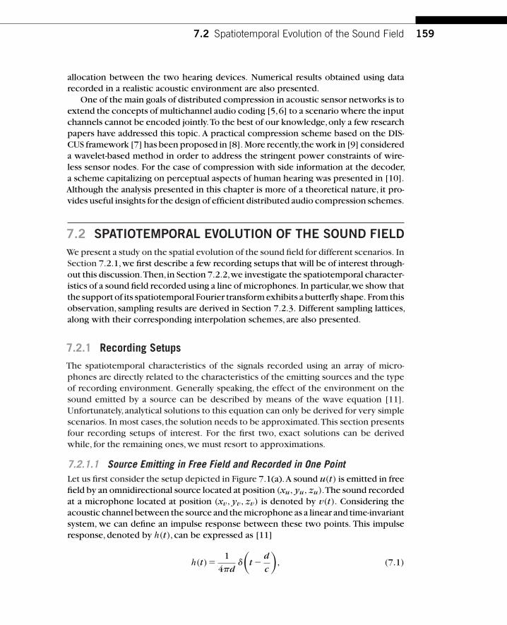
7.2 Spatiotemporal Evolution of the Sound Field 159
allocation between the two hearing devices. Numerical results obtained using datarecorded in a realistic acoustic environment are also presented.
One of the main goals of distributed compression in acoustic sensor networks is toextend the concepts of multichannel audio coding [5,6] to a scenario where the inputchannels cannot be encoded jointly.To the best of our knowledge,only a few researchpapers have addressed this topic. A practical compression scheme based on the DIS-CUS framework [7] has been proposed in [8]. More recently,the work in [9] considereda wavelet-based method in order to address the stringent power constraints of wire-less sensor nodes. For the case of compression with side information at the decoder,a scheme capitalizing on perceptual aspects of human hearing was presented in [10].Although the analysis presented in this chapter is more of a theoretical nature, it pro-vides useful insights for the design of efficient distributed audio compression schemes.
7.2 SPATIOTEMPORAL EVOLUTION OF THE SOUND FIELDWe present a study on the spatial evolution of the sound field for different scenarios. InSection 7.2.1,we first describe a few recording setups that will be of interest through-out this discussion.Then,in Section 7.2.2,we investigate the spatiotemporal character-istics of a sound field recorded using a line of microphones. In particular,we show thatthe support of its spatiotemporal Fourier transform exhibits a butterfly shape. From thisobservation, sampling results are derived in Section 7.2.3. Different sampling lattices,along with their corresponding interpolation schemes, are also presented.
7.2.1 Recording Setups
The spatiotemporal characteristics of the signals recorded using an array of micro-phones are directly related to the characteristics of the emitting sources and the typeof recording environment. Generally speaking, the effect of the environment on thesound emitted by a source can be described by means of the wave equation [11].Unfortunately,analytical solutions to this equation can only be derived for very simplescenarios. In most cases, the solution needs to be approximated.This section presentsfour recording setups of interest. For the first two, exact solutions can be derivedwhile, for the remaining ones, we must resort to approximations.
7.2.1.1 Source Emitting in Free Field and Recorded in One PointLet us first consider the setup depicted in Figure 7.1(a).A sound u(t) is emitted in freefield by an omnidirectional source located at position (xu, yu, zu).The sound recordedat a microphone located at position (xv, yv, zv) is denoted by v(t). Considering theacoustic channel between the source and the microphone as a linear and time-invariantsystem, we can define an impulse response between these two points. This impulseresponse, denoted by h(t), can be expressed as [11]
h(t)�1
4�d�
(t �
d
c
), (7.1)
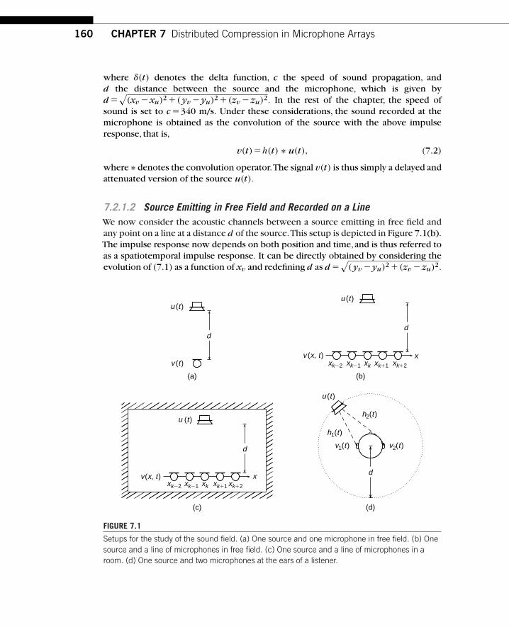
160 CHAPTER 7 Distributed Compression in Microphone Arrays
where �(t) denotes the delta function, c the speed of sound propagation, andd the distance between the source and the microphone, which is given byd �
√(xv �xu)2 �( yv �yu)2 �(zv �zu)2. In the rest of the chapter, the speed of
sound is set to c �340 m/s. Under these considerations, the sound recorded at themicrophone is obtained as the convolution of the source with the above impulseresponse, that is,
v(t)�h(t) ∗ u(t), (7.2)
where ∗ denotes the convolution operator.The signal v(t) is thus simply a delayed andattenuated version of the source u(t).
7.2.1.2 Source Emitting in Free Field and Recorded on a LineWe now consider the acoustic channels between a source emitting in free field andany point on a line at a distance d of the source.This setup is depicted in Figure 7.1(b).The impulse response now depends on both position and time,and is thus referred toas a spatiotemporal impulse response. It can be directly obtained by considering theevolution of (7.1) as a function of xv and redefining d as d �
√( yv �yu)2 �(zv �zu)2.
v (t)
u (t)
d
(a)
xk22 xk21 xk xk11xk12
v (x, t )xk22 xk21 xk xk11 xk12
x
u (t)
d
(b)
v(x, t ) x
u (t )
d v1(t ) v2(t )
u (t )
d
h1(t)
h2(t )
(d)(c)
FIGURE 7.1
Setups for the study of the sound field. (a) One source and one microphone in free field. (b) Onesource and a line of microphones in free field. (c) One source and a line of microphones in aroom. (d) One source and two microphones at the ears of a listener.

7.2 Spatiotemporal Evolution of the Sound Field 161
0 32.5
1.5
0.5
20.521
2Position (m)
Time (s)
00.5
1
1
0
0.0020.004
0.0060.008
0.010.012
0.0140.016
0.0180.02
0 32.5
1.5
0.5
20.521
2Position (m)
Time (s)
00.5
1
1
0
0.0020.004
0.0060.008
0.010.012
0.0140.016
0.0180.02
(a) (b)
FIGURE 7.2
Theoretical spatiotemporal impulse response on a line. (a) In free field. (b) Inside a room. Thespatiotemporal impulse response inside a room is obtained using the image method (seeSection 7.2.1.3).
For simplicity, we denote the variable xv by x such that the spatiotemporal impulseresponse can be expressed as
h(x, t)�1
4�√
(x �xu)2 �d2�
(t �
√(x �xu)2 �d2
c
). (7.3)
The function h(x, t) is plotted in Figure 7.2(a). The signal v(x0, t) recorded at a fixedposition x0 on the line can thus be obtained as the (one-dimensional) convolutionof the impulse response at position x0, given by h(x0, t), with the source u(t). Inthis scenario, referred to as near-field, both the delay and the attenuation depend onthe distance between the source and the microphone. To simplify matters, it is oftenassumed [12, 13] that the source is far enough away from the microphones such thatthe wave front impinging on the line of microphones appears as a plane wave. Thisassumption is known as the far-field assumption. In this case, the delay only dependson the direction of propagation of the wave. Moreover, the attenuation is assumedto be constant across microphones and is set to unity. The spatiotemporal impulseresponse (7.3) hence reduces to
h(x, t)��(t �
x cos �
c
), (7.4)
where � denotes the angle of arrival of the plane wave (see Figure 7.3(a)).
7.2.1.3 Source Emitting in a Room and Recorded on a LineLet us now turn our attention to the recording setup illustrated in Figure 7.1(c). Thesource no longer emits in free field but instead emits inside a rectangular room. In room

162 CHAPTER 7 Distributed Compression in Microphone Arrays
x
y
�
(a)
V
F1
2 ccos �
(b)
V
F1
c
(c)
FIGURE 7.3
Far-field assumption for the spatiotemporal study of the sound field. (a) Plane wave impinging ona line of microphones with angle �. (b) Support of the 2D spectrum of the spatiotemporal impulseresponse. (c) If one considers all possible angles of arrival, the spectral support of thespatiotemporal impulse response has a butterfly shape.
acoustics,the impulse response is referred to as a room impulse response (RIR). It canbe directly measured (e.g., see [14]) or estimated using a parametric model.The mostcommon approach for simulating RIRs for simple geometries is the image method [15].The idea is to model the reflections of the sound on the walls as new virtual sourceslocated on the far side of these walls. Reverberation in a room is thus modeled byadding the effect of a large number of virtual free-field sources (theoretically an infinitenumber).The RIR is obtained by adding the impulse responses corresponding to eachof these virtual sources. A spatiotemporal RIR on a line simulated using the imagesource model is shown in Figure 7.2(b).
7.2.1.4 Source Emitting in Free Field and Recorded at the Ears of a ListenerWe assume now that the source is recorded at the left and right ears of a listener,as depicted in Figure 7.1(d). The direction-dependent transfer characteristics from asound source to the ear is called head-related impulse response (HRIR) in the time-domain representation and head-related transfer function (HRTF) in the frequency-domain representation. These functions describe the acoustic filtering, due to thepresence of a listener, of a sound wave propagating in free field. The HRTF is definedas the ratio between the Fourier transform of the sound pressure at the entrance ofthe ear canal and the one in the middle of the head in the absence of the listener [16].HRTFs are therefore filters quantifying the effect of the shape of the head, body, andpinnae on the sound arriving at the entrance of the ear canal. A typical situation isdescribed in Figure 7.1(d). The source emits the sound u(t) in free field. The HRIRsdescribing the filters between the source and the left and right ears are denoted byh1(t) and h2(t), respectively. The sound signals recorded at the ears, denoted by v1(t)and v2(t), are again obtained by convolution. Many models exist for simulating HRTFs(e.g.,see [17]).These models mostly consider the diffraction effect of the sound aroundthe head. In this scenario, the head reduces the intensity of the sound arriving at thecontralateral ear, a phenomenon commonly referred to as head shadowing.
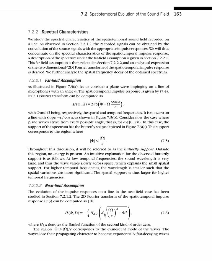
7.2 Spatiotemporal Evolution of the Sound Field 163
7.2.2 Spectral Characteristics
We study the spectral characteristics of the spatiotemporal sound field recorded ona line. As observed in Section 7.2.1.2, the recorded signals can be obtained by theconvolution of the source signals with the appropriate impulse responses.We will thusconcentrate on the spectral characteristics of the spatiotemporal impulse response.A description of the spectrum under the far-field assumption is given in Section 7.2.2.1.This far-field assumption is then relaxed in Section 7.2.2.2,and an analytical expressionof the two-dimensional (2D) Fourier transform of the spatiotemporal impulse responseis derived. We further analyze the spatial frequency decay of the obtained spectrum.
7.2.2.1 Far-field AssumptionAs illustrated in Figure 7.3(a), let us consider a plane wave impinging on a line ofmicrophones with an angle �.The spatiotemporal impulse response is given by (7.4).Its 2D Fourier transform can be computed as
H(�, �)�2��(
���cos �
c
),
with � and � being,respectively,the spatial and temporal frequencies. It is nonzero ona line with slope �c/ cos �, as shown in Figure 7.3(b). Consider now the case whereplane waves arrive from every possible angle, that is, for �∈[0, 2�). In this case, thesupport of the spectrum has the butterfly shape depicted in Figure 7.3(c).This supportcorresponds to the region where
|�|� |�|c
. (7.5)
Throughout this discussion, it will be referred to as the butterfly support. Outsidethis region, no energy is present. An intuitive explanation for the observed butterflysupport is as follows. At low temporal frequencies, the sound wavelength is verylarge, and thus the wave varies slowly across space, which explains the small spatialsupport. For higher temporal frequencies, the wavelength is smaller such that thespatial variations are more significant. The spatial support is thus larger for highertemporal frequencies.
7.2.2.2 Near-field AssumptionThe evolution of the impulse responses on a line in the near-field case has beenstudied in Section 7.2.1.2. The 2D Fourier transform of the spatiotemporal impulseresponse (7.3) can be computed as [18]
H(�, �)��j
4H2,0
⎛⎝d
√(�
c
)2
��2
⎞⎠, (7.6)
where H2,0 denotes the Hankel function of the second kind of order zero.The region |�|� |�|/c corresponds to the evanescent mode of the waves. The
waves lose their propagating character to become exponentially fast-decaying waves
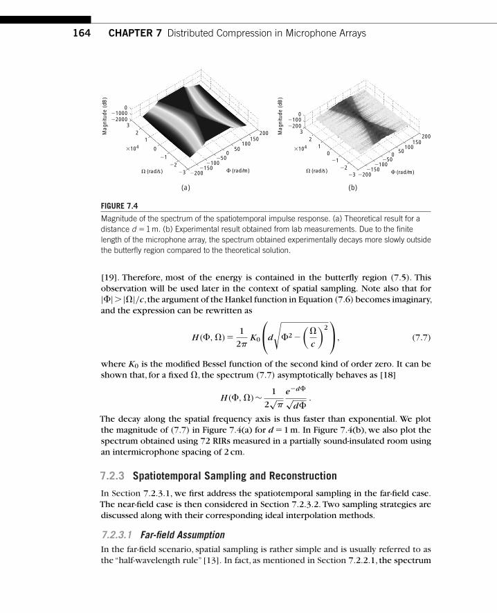
164 CHAPTER 7 Distributed Compression in Microphone Arrays
Mag
nitu
de (
dB)
2122
23 22002150
2100F (rad/m)V (rad/s)
3104
250
500
100150
200
02100022000
32
1
0
Mag
nitu
de (
dB)
021002200
2122
23 22002150
2100F (rad/m)V (rad/s)
3104
250
500
100150
2003
21
0
(a) (b)
FIGURE 7.4
Magnitude of the spectrum of the spatiotemporal impulse response. (a) Theoretical result for adistance d �1 m. (b) Experimental result obtained from lab measurements. Due to the finitelength of the microphone array, the spectrum obtained experimentally decays more slowly outsidethe butterfly region compared to the theoretical solution.
[19]. Therefore, most of the energy is contained in the butterfly region (7.5). Thisobservation will be used later in the context of spatial sampling. Note also that for|�|� |�|/c,the argument of the Hankel function in Equation (7.6) becomes imaginary,and the expression can be rewritten as
H(�, �)�1
2�K0
⎛⎝d
√�2 �
(�
c
)2⎞⎠, (7.7)
where K0 is the modified Bessel function of the second kind of order zero. It can beshown that, for a fixed �, the spectrum (7.7) asymptotically behaves as [18]
H(�, �)∼ 1
2√
�
e�d�
√d�
.
The decay along the spatial frequency axis is thus faster than exponential. We plotthe magnitude of (7.7) in Figure 7.4(a) for d �1 m. In Figure 7.4(b), we also plot thespectrum obtained using 72 RIRs measured in a partially sound-insulated room usingan intermicrophone spacing of 2 cm.
7.2.3 Spatiotemporal Sampling and Reconstruction
In Section 7.2.3.1, we first address the spatiotemporal sampling in the far-field case.The near-field case is then considered in Section 7.2.3.2. Two sampling strategies arediscussed along with their corresponding ideal interpolation methods.
7.2.3.1 Far-field AssumptionIn the far-field scenario, spatial sampling is rather simple and is usually referred to asthe “half-wavelength rule” [13]. In fact, as mentioned in Section 7.2.2.1, the spectrum
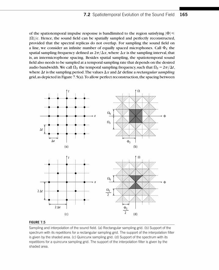
7.2 Spatiotemporal Evolution of the Sound Field 165
of the spatiotemporal impulse response is bandlimited to the region satisfying |�|�|�|/c. Hence, the sound field can be spatially sampled and perfectly reconstructed,provided that the spectral replicas do not overlap. For sampling the sound field ona line, we consider an infinite number of equally spaced microphones. Call �S thespatial sampling frequency defined as 2�/x,where x is the sampling interval, thatis, an intermicrophone spacing. Besides spatial sampling, the spatiotemporal soundfield also needs to be sampled at a temporal sampling rate that depends on the desiredaudio bandwidth. We call �S the temporal sampling frequency, such that �S �2�/t ,where t is the sampling period.The values x and t define a rectangular samplinggrid,as depicted in Figure 7.5(a).To allow perfect reconstruction,the spacing between
x
t
Dt
Dx
2Dt
2Dx
(a)
V0
V0
VS
FS
F
F
V
V
(b)
x
t
(c) (d)
VS
2
FS
2
FIGURE 7.5
Sampling and interpolation of the sound field. (a) Rectangular sampling grid. (b) Support of thespectrum with its repetitions for a rectangular sampling grid. The support of the interpolation filteris given by the shaded area. (c) Quincunx sampling grid. (d) Support of the spectrum with itsrepetitions for a quincunx sampling grid. The support of the interpolation filter is given by theshaded area.

166 CHAPTER 7 Distributed Compression in Microphone Arrays
consecutive microphones must be at most equal to
x ��c
�0,
where �0 denotes the maximum temporal frequency. Equivalently, the minimumspatial sampling frequency is equal to
�S �2�
x�
2�0
c.
It can be directly observed from Figure 7.5(b) that, under this condition, the spectralreplicas do not overlap.The original sound field can thus be recovered using standardinterpolation techniques (e.g.,see [20]).The interpolation filter, in this case, is an ideallow-pass filter whose support is shown in bold in Figure 7.5(b).
A tighter packing of the spectrum can be achieved by using quincunx sampling.In time domain, the grid to be used is shown in Figure 7.5(c). In the correspondingspectrum,the spectral replicas are placed such that they fill the whole frequency planeas shown in Figure 7.5(d). With quincunx sampling, the temporal sampling frequencycan be halved, while preserving the perfect reconstruction property. In this case, theeven microphones are sampled at even times while the odd microphones are sampledat odd times.This leads to a gain factor of two in the processing. However, it does notreduce the necessary number of microphones.The ideal interpolation filter in this caseis referred to as a “fan filter” [21] whose support is indicated in bold in Figure 7.5(d).
7.2.3.2 Near-field AssumptionIn the near-field scenario,the situation is different. Let us consider the spectrum of thespatiotemporal impulse response given by (7.6) at a particular temporal frequency �0.It has approximately the shape given in Figure 7.6(a). In particular, it is not bandlim-ited. When the sound field is sampled, repetitions of the spectrum occur as shown inFigure 7.6(b). As the spectrum is not perfectly bandlimited, the repetitions will affectthe reconstruction; that is, aliasing will occur. To quantify this effect, we consider thesignal-to-noise ratio (SNR) of the reconstructed sound field. Let SNR(�S, �0) denotethe SNR of the reconstructed sound field corresponding to a sinusoid emitted at fre-quency �0 and where the spatial sampling frequency of the microphone array is �S .We define this SNR as
SNR(�S, �0)�
∫ � |H(�, �0)|2 d�
4∫
�S/2 |H(�, �0)|2 d�. (7.8)
The numerator in Equation (7.8) corresponds to the energy of the spectrum at temporalfrequency �0. The denominator contains two different kinds of energy: the in-bandenergy and the out-of-band energy.The in-band energy corresponds to the energy of allthe spectral replicas that contaminate the domain of interest, that is, [��S/2, �S/2].The out-of-band energy is the energy present in the original spectrum that is outsidethe domain of interest. It can be shown that these two energies are equal in the case of

7.2 Spatiotemporal Evolution of the Sound Field 167
F
F
(a)
|H (F, V0)|
|H (F, V0)|
2
(b)
FS
2
FS
2
FIGURE 7.6
Magnitude of the spectrum of the spatiotemporal impulse response for a particular temporalfrequency �0. (a) Original spectrum. (b) Replicated spectrum after spatial sampling. We observethat the replicas overlap with the original spectrum, preventing perfect reconstruction.
an infinite line of microphones.This explains the factor 4 in the denominator of (7.8).The SNR evaluates as [18]
SNR(�S, �0)�1
2d∫
�S/2
∣∣∣∣∣H2,0
(d
√(�0c
)2��2
)∣∣∣∣∣2
d�
. (7.9)
The computation of the SNR (7.9) is rather involved. For �S �2�0/c, however, it canbe lower bounded by [18]
SNR(�S, �0)��
4Ei
(2d
√(�S2
)2�(
�0c
)2) , (7.10)
where Ei denotes the exponential integral function defined as Ei(x)�∫
xe�t
t dt . As anumerical check of the tightness of the bound,the SNR (7.9) and its lower bound (7.10)
are plotted in Figure 7.7 as a function of the normalized sampling frequency �S d,for different normalized temporal frequencies �0 d. For a given normalized temporalfrequency,it can be observed that the SNR increases as the normalized spatial samplingfrequency increases. We also observe that the lower bound tightly follows the exact

168 CHAPTER 7 Distributed Compression in Microphone Arrays
V0d51
0 10 20 30 40 50 60220
0
20
40
60
80
100
120
FSd (rad)
SN
R (
dB)
SNRLower bound
V0d 5 2000 V0d 5 4000 V0d 5 6000 V0d 5 8000
FIGURE 7.7
Reconstruction SNR and its lower bound as a function of the normalized spatial samplingfrequency �Sd. The different sets of curves correspond to different normalized temporalfrequencies �0d.
Table 7.1 Minimum Intermicrophone Spacing (in cm) for DifferentTemporal Frequencies �0 and Different SNR Requirements. The Distanceis d =1 m
Far Field Near Field
20 dB 40 dB 60 dB 80 dB 100 dB
2000 rad/s (318 Hz) 53.41 51.30 45.31 38.14 31.84 26.86
8000 rad/s (1.3 kHz) 13.35 13.32 13.19 12.97 12.65 12.27
15,000 rad/s (2.4 kHz) 7.12 7.12 7.10 7.06 7.01 6.94
20,000 rad/s (3.2 kHz) 5.34 5.34 5.33 5.32 5.29 5.27
SNR computed using (7.9). It can be computed from (7.10) that to reconstruct thesound field at a temporal frequency of 8000 rad/s (1.3 kHz), a spatial distance of12.35 cm is sufficient to achieve a reconstruction quality of 100 dB when a unitdistance between the source and the line of microphones is considered. Under thefar-field assumption, the required spacing to obtain perfect reconstruction would be13.35 cm. Further numerical examples are provided in Table 7.1.

7.3 Huygens’s Configuration 169
Similarly to the far-field scenario, quincunx sampling may be used to achieve atighter packing of the spectrum, and an SNR formula similar to (7.9) may be derived.
7.3 HUYGENS’S CONFIGURATIONLet us now turn our attention to the distributed compression problem of audio signals.The first setup of interest consists of an infinite number of sensors equally spaced on aline. They record a continuous, stationary, Gaussian sound field that is emitted from aline parallel to the recording line.This setup is motivated by the following observation.According to Huygens’s principle [22], a wave front generated by a sound source canbe replaced by an infinite number of point sources placed on the wave front. Thisprinciple is at the basis of wave field synthesis [23]. If this sound source is sufficientlyfar away from the recording devices, the far-field assumption allows neglecting thecurvature of the wave front such that it reduces to a line. For this reason, we refer tothe considered setup as Huygens’s configuration. Closed-form rate-distortion formulasare obtained for various sampling lattices and coding strategies. In particular,we showthat, under a whiteness requirement, the best achievable rate distortion trade-off canbe obtained by judicious signal processing at the sensors. We thus provide, for thisparticular example, the solution to the multiterminal source coding problem.
7.3.1 Setup
The recording setup is illustrated in Figure 7.8(a). Sound sources distributed on aninfinite line U emit a spatiotemporal acoustic field U (x, t). The sound field U (x, t) isassumed to be a zero-mean Gaussian random field that is stationary across both spaceand time. We denote its power spectral density by SU (�, �). Recall that the variables� and � refer to the spatial and temporal frequencies, respectively. The field U (x, t)induces a sound field V (x, t) recorded on a line V , parallel to and at a distance dfrom the line U . The field V (x, t) can be written as the convolution of U (x, t) with
U x
V x
U (x, t )
V (x, t )
dh (x, t )
(a)
V x
Base station
V(x, t )
(b)
xk�2 xk�1 xk xk�1 xk�2
ˆ
FIGURE 7.8
Huygens’s configuration. (a) Sound field propagation setup. (b) Spatiotemporal sampling anddistributed coding setup.

170 CHAPTER 7 Distributed Compression in Microphone Arrays
the space and time invariant filter h(x, t), which we obtain from (7.3). The processV (x, t) is thus also a stationary Gaussian random field with mean zero and a powerspectral density given by [24]
SV (�, �)� |H(�, �)|2SU (�, �), (7.11)
where H(�, �) is the 2D Fourier transform of h(x, t) derived in (7.6). In particular,the spatiotemporal bandwidth of SV (�, �) is given by the intersection of the supportsof H(�, �) and SU (�, �).
As depicted in Figure 7.8(b), sensors located on the recording line V sample thesound field V (x, t),encode their observation at a given rate,and transmit the quantizedsamples to a base station. More specifically, the sensor k samples the field V (x, t) atposition xk and time instants tk(n), for k, n∈Z. The values xk and tk(n) define thesampling lattice. In the sequel, we will consider the rectangular and the quincunxlattices introduced in Section 7.2.3. The samples are then encoded into a bitstreamthat is transmitted to the base station.The goal of the base station is to provide,basedon the received data, an estimate V (x, t) of the recorded sound field V (x, t) for anyposition on the recording line and any time instant. The average rate R used by thesensors is measured in bits per meter per second, and the average distortion D is themean-squared error (MSE) between V (x, t) and V (x, t) per meter and per second. Ourinterest lies in the determination of rate-distortion functions under various simplifyingassumptions on the spectral characteristics of the sound fields and under differentconstraints on the communication allowed between the sensors.
7.3.2 Coding Strategies
We consider the three coding strategies depicted in Figure 7.9. The first one, referredto as centralized coding (see Figure 7.9(a)), assumes that there is one encoder thathas access to the measurements of all the sensors and can encode them jointly. Forinstance,we may assume the existence of a genie informing each sensor about the othersensors’ measurements or, more realistically, the existence of unconstrained commu-nication links between the sensors, which can be used without any cost (e.g., wiredmicrophones). In the second coding strategy, referred to as spatially independentcoding (see Figure 7.9(b)), each sensor encodes its samples, ignoring the correlationwith the data measured by neighboring sensors. Similarly,the base station decodes thebitstream received from each sensor separately. In the last coding strategy, referred toas multiterminal coding (see Figure 7.9(c)), each sensor encodes its data separatelybut takes into account the intersensor correlation that is assumed to be known. Thebase station decodes the received bitstreams jointly. The rate-distortion function in thiscase is lower bounded by the rate-distortion function with centralized coding,becauseany scheme that works in the former scenario can also be applied in the latter. Sim-ilarly, it is upper bounded by the rate-distortion function with spatially independentcoding since intersensor correlation is taken into account.The first two strategies thusprovide bounds on the rate-distortion function of the multiterminal scenario whosegeneral characterization remains unknown to date.

7.3 Huygens’s Configuration 171
V (x, t )
V (x1, t )
V (x2, t )
V (xK, t )
V (x, t )
V (x1, t )
V (x2, t )
V (xK, t )
V (x1, t )
V (x2, t )
V (xK, t )
V (x1, t )V (x2, t )
V (xK, t )
Encoder Decoder
(a)
Decoder 1
Decoder 2
Decoder K
(b)
Encoder 1
Encoder 1
Encoder 2
Encoder 2
Encoder K
Encoder K
Decoder
(c)
FIGURE 7.9
The three coding strategies considered for Huygens’s configuration. (a) Centralized coding.(b) Spatially independent coding. (c) Multiterminal coding.
The assumption of known intersensor correlation is a strong one, for it may bedifficult to compute such statistics in a practical setting. Coding methods that do notrely on such prior knowledge are thus of particular interest. In the sequel, we willshow that, under simplifying assumptions, it is possible to achieve the lower boundgiven by centralized coding using an appropriate quincunx sampling lattice followedby independent coding.
7.3.3 Rate-distortion Trade-offs
In order to derive closed-form rate-distortion functions for the different coding strate-gies considered in Section 7.3.2, we will make two simplifying assumptions. First, weassume that H(�, �) is zero outside the butterfly region. This corresponds to the far-field assumption (see Section 7.2.2.1) and is thus a good approximation of the truesupport when d is large. In this case, it follows from (7.11) that for a source U (x, t)

172 CHAPTER 7 Distributed Compression in Microphone Arrays
with maximum temporal frequency �0, the maximum spatial frequency of V (x, t) isgiven by �0 ��0/c, regardless of the actual spatial bandwidth of U (x, t). The secondassumption is that the power spectral density of the recorded sound field V (x, t) isconstant over its support and is given by �2
V .This assumption is a worst-case scenarioin the sense that, for given bandwidth and total power, the Gaussian random field thatrequires the highest bit rate for centralized coding is the one with a constant powerspectral density. Under these assumptions,we obtain the following optimal rate distor-tion trade-offs in closed form. For centralized coding, the rate-distortion function canbe readily derived from standard results on compression of Gaussian random processes(e.g., see [25, 26]) as
Rc(D)��2
0
4�2clog
(�2
V �20
2�2cD
). (7.12)
For spatially independent coding and the rectangular sampling lattice, we obtain [27]
Rr(D)��2
0
2�2clog
[�2
V �20
e�2cD
1
2
(1�
√1�2
�2cD
�2V �2
0
)]
��2
0
2�2c
(1�
√1�2
�2cD
�2V �2
0
).
(7.13)
For spatially independent coding and the quincunx sampling lattice, we find [27]
Rq(D)��2
0
4�2clog
(�2
V �20
2�2cD
). (7.14)
In the above equations,D∈(0, (�2V �2
0)/(2�2c)). The important point regarding these
rate-distortion functions is that the expressions (7.12) and (7.14) coincide. In otherwords, the strategy of sampling with a quincunx lattice followed by spatially indepen-dent coding achieves the lower bound given by the centralized scenario and hencedetermines the multiterminal rate-distortion function for this setup.This can be intui-tively explained by the fact that the quincunx lattice allows for a perfect tiling of thefrequency plane as shown in Figure 7.5(d). This results in a sampled spatiotemporalfield whose power spectral density is flat. The processes sampled at each sensor areuncorrelated and can thus be encoded independently without any loss in terms ofthe rate-distortion trade-off. It is important to note that the sensor observations can-not be made independent using, for example, a transform coding approach [28, 29],because the measurements cannot be processed jointly. Under our assumptions,how-ever, quincunx sampling achieves the same goal without the need for centralizedprocessing. We plot the above rate-distortion functions in Figure 7.10. Note that thesampling lattice in this example is chosen as a function of the temporal and spatialbandwidth such as to obtain a perfect tiling of the frequency plane. If the sensor
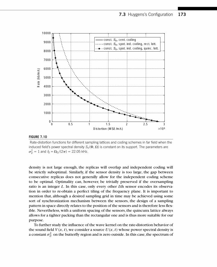
7.3 Huygens’s Configuration 173
0 0.5 1 1.5 2 2.5 3�106
0
1000
2000
3000
4000
5000
6000
7000
8000
9000
10000
Distortion (MSE/m/s)
Rat
e (k
b/m
/s)
const. SV, cent. codingconst. SV, spat. ind. coding, rect. latt.const. SV, spat. ind. coding, quinc. latt.
FIGURE 7.10
Rate-distortion functions for different sampling lattices and coding schemes in far field when theinduced field’s power spectral density SV (�, �) is constant on its support. The parameters are�2
V � 1 and f0 � �0/(2�) � 22.05 kHz.
density is not large enough, the replicas will overlap and independent coding willbe strictly suboptimal. Similarly, if the sensor density is too large, the gap betweenconsecutive replicas does not generally allow for the independent coding schemeto be optimal. Optimality can, however, be trivially preserved if the oversamplingratio is an integer L. In this case, only every other Lth sensor encodes its observa-tion in order to re-obtain a perfect tiling of the frequency plane. It is important tomention that, although a desired sampling grid in time may be achieved using somesort of synchronization mechanism between the sensors, the design of a samplingpattern in space directly relates to the position of the sensors and is therefore less flex-ible. Nevertheless, with a uniform spacing of the sensors, the quincunx lattice alwaysallows for a tighter packing than the rectangular one and is thus more suitable for ourpurpose.
To further study the influence of the wave kernel on the rate-distortion behavior ofthe sound field V (x, t),we consider a source U (x, t) whose power spectral density isa constant �2
U on the butterfly region and is zero outside. In this case, the spectrum of

174 CHAPTER 7 Distributed Compression in Microphone Arrays
0 20 40 60 80 100 120 1400
1000
2000
3000
4000
5000
6000
7000
8000
9000
Distortion (MSE/m/s)
Rat
e (k
b/m
/s)
const. SU, cent. codingconst. SU, spat. ind. coding, rect. latt.const. SU, spat. ind. coding, quinc. latt.
FIGURE 7.11
Rate-distortion functions for different sampling lattices and coding schemes in far field when thesource field’s power spectral density SU(�, �) is constant on its support. The parameters ared �100 m, �2
U �1 and f0 � �0/(2�) � 22.05 kHz.
the induced field V (x, t) follows from (7.11) and is no longer constant on the butterflysupport. We thus resort to numerical integration to compute the corresponding rate-distortion functions depicted in Figure 7.11. Unlike the previous case,where SV (�, �)
is constant on the butterfly support,the spatially independent coding scheme with thequincunx sampling lattice does not achieve the performance of the centralized codingscheme, but it still outperforms the scheme with the rectangular sampling lattice bya significant margin. Hence, by adjusting the sampling lattice to the wave kernel’sspectral properties, we achieve a good performance even with a coding scheme thattreats the sensor measurements independently.This observation motivates the generaladvice that the communication schemes should be tailored to the physical propertiesof the problem under consideration.
Another way of getting a tighter packing of the replicas of SV (�, �), while pre-serving a rectangular lattice, consists in decomposing the sound field into M spectralsubbands by filtering in the temporal domain, as shown in Figure 7.12. Each of thesubband fields is sampled using a rectangular sampling lattice adjusted to the spatialand temporal bandwidths of the particular subband. This implementation generally

7.3 Huygens’s Configuration 175
�0/2
��0/2
�
�
�0
��0
�
2�0/4
�2�0/4
2�0/3
�2�0/3
2�0/5
�2�0/5
V (2)
V (2)
V (3)
V (3)
V (4)
V (4)
V (1)
V (1)
V (2)
V (2)
V (1)
V (1)
��0
�0
�
(a) (b)
FIGURE 7.12
Spectral decomposition of the sound field by filtering in the temporal domain. (a) L�1 and M�2.(b) L�2 and M�4.
requires the deployment of additional sensors with appropriate intersensor spacingsfor each subband field. A uniform sensor deployment can, however, still be preservedby considering an L-times higher sensor density, for some integer L. More precisely,the intersensor spacing is chosen as x/L, where x ��c/�0 denotes the spacing atthe Nyquist rate. We then define the subband field V (m)(x, t) as the field obtained byideal bandpass filtering V (x, t) on a pass-band given by⎧⎪⎪⎪⎪⎨⎪⎪⎪⎪⎩
[�
L�0
L�m�1, �
L�0
L�m
]∪[
L�0
L�m,
L�0
L�m�1
]for m�1, . . . , M �1,[
�L�0
L�M �1,
L�0
L�M �1
]for m�M .
Note that this scheme only requires temporal filtering (recall that spatial filtering isimpossible in practice). Figure 7.12 shows the resulting decompositions for L�1 andM �2 (see Figure 7.12(a)) as well as for L�2 and M �4 (see Figure 7.12(b)).The spa-tial bandwidth of V (m)(x, t) is 2L�0/
(c(L�m�1)
), thus, V (m)(x, t) can be sampled
with an intersensor spacing of (L�m�1)x/L. This sampling rate is obtained byhaving one sensor out of L�m�1 record the samples of the subband field V (m)(x, t).The sensors apply the spatially independent coding scheme defined in Section 7.3.2to each sampled subband field. Since the spectral densities of the subband signalshave nonoverlapping supports, these random fields are uncorrelated, and thus, theymay be encoded independently without any penalty in terms of the rate-distortiontrade-off. This is provided that the rate allocation among the subbands is performedaccording to the reverse water-pouring principle [25, 26].
To illustrate the performance of the subband coding scheme defined earlier,we firstconsider the decomposition of the sound field into two subbands of equal width, as

176 CHAPTER 7 Distributed Compression in Microphone Arrays
0 0.5 1 1.5 2 2.5 33 106
0
1000
2000
3000
4000
5000
6000
7000
8000
9000
10000
Distortion (MSE/m/s)
Rat
e (k
b/m
/s)
centralized codingspat. indep. coding, rect. latt.subband coding, L 5 1, M 5 2
FIGURE 7.13
Rate-distortion function for the subband coding scheme with L�1 and M�2. The spectraldensity SV (�, �) is chosen constant on its support. The parameters are �2
V �1 andf0 � �0/(2�) � 22.05 kHz.
shown in Figure 7.12(a).The sensors are deployed with an intersensor spacing of x,and the subband field V (2)(x, t) is sampled by every other sensor. Figure 7.13 shows theresulting rate-distortion curve in comparison with the ones for centralized coding andfor spatially independent coding with the rectangular sampling lattice. Observe that,without deploying additional sensors, we can improve the performance of the latterscheme by combining it with the subband decomposition method. Next,we considerthe spectral subdivision into multiple subbands. For a given value of the parameter L,we choose M �9L�1,so that the temporal bandwidth of the subband field V (M)(x, t)is equal to �0/5. Note that increasing the parameter L requires a proportional increaseof the sensor density, whereas an increase of the number of subbands M only addsto the local processing complexity. Figure 7.14 shows the resulting rate-distortioncurves for L�1, 2, 3. Observe that, with a moderate increase of the sensor density,the performance of the spatially independent coding scheme with the rectangularsampling lattice combined with the subband decomposition method approaches theone of centralized coding.

7.4 Binaural Hearing Aid Configuration 177
0 0.5 1 1.5 2 2.5 3� 106
0
1000
2000
3000
4000
5000
6000
7000
8000
9000
10000
Distortion (MSE/m/s)
Rat
e (k
b/m
/s)
centralized codingspat. indep. coding, rect. latt.subband coding, L�1, M�10subband coding, L�2, M�19subband coding, L�3, M�28
FIGURE 7.14
Rate-distortion functions for the subband coding scheme with L � 1,2,3 and M � 9L�1. Thespectral density SV (�, �) is chosen constant on its support. The parameters are �2
V �1 andf0 � �0/(2�) � 22.05 kHz.
7.4 BINAURAL HEARING AID CONFIGURATIONThe distributed compression scenario considered in this section involves only two sen-sors,namely, two digital hearing aids (left and right) allowed to exchange compressedaudio signals by means of a wireless link.The setup is referred to as the binaural hear-ing aid configuration. The study of optimal rate-distortion trade-offs in this contextallows quantifying the noise reduction provided by the availability of a rate-constrainedcommunication medium between the two hearing instruments. Closed-form rate-distortion formulas are derived in a simple yet insightful scenario, along with optimalrate-allocation strategies. More realistic acoustic environments are discussed,for whichnumerical results are presented.
7.4.1 Setup
Let us consider the binaural hearing aid configuration depicted in Figure 7.15. A usercarries a left and a right hearing aid,both comprising a set of microphones,a processing

178 CHAPTER 7 Distributed Compression in Microphone Arrays
V1(t) V2(t)
(a) (b)
V1(t) Proc Proc
Trans Trans
V2(t)
FIGURE 7.15
Binaural hearing aid configuration. (a) Recording setup. (b) Collaborative processing usingwireless links.
unit with wireless communication capabilities, and a loudspeaker. For simplicity ofexposure, we will consider that only one microphone is available at each hearingdevice, and we will denote the signal recorded at microphone k by Vk(t) for k�1, 2.We assume that Vk(t) can be decomposed into a speech (or desired) component,denoted V s
k(t), and an additive noise (or undesired) component, denoted V nk (t), as
Vk(t)�V sk(t)�V n
k (t) for k�1, 2. (7.15)
For the sake of mathematical tractability, the speech and noise signals are modeled asindependent, zero-mean, stationary Gaussian random processes.
The goal of each hearing instrument is to recover the speech component of itsmicrophone with minimum MSE.To make matters clearer,let us adopt the perspectiveof hearing aid 1. It aims at estimating the signal V s
1 (t) with minimum MSE based onits own observation V1(t) and a compressed version of the signal V2(t) recordedat hearing aid 2. With the above considerations, the setup simply corresponds to aremote source coding problem with side information at the decoder. This problem,alsoreferred to as indirect or noisy Wyner–Ziv coding in the literature,has been addressedby various researchers in the scalar case [30–32]. More generally,Witsenhausen [33]elegantly demonstrated how certain classes of remote rate-distortion problems canbe reduced to direct ones, unifying earlier results by Dobrushin and Tsybakov [34],Sakrison [35], and Wolf and Ziv [36]. Extension to vector sources was investigatedby Rebollo-Monedero et al. in the context of high-rate transform coding [37]. In thecontinuous-time case, we wish to encode V2(t) with rate R1 such as to minimizethe distortion D1 between V s
1 (t) and its reconstruction V s1 (t), assuming the presence
of the side information V1(t) at the decoder. The rate R1 is measured in bits persecond and the distortion D1 in MSE per second. This procedure is illustrated forboth devices in Figure 7.16. As in Section 7.3, our goal is to determine rate-distortionfunctions under two different coding strategies and various simplifying assumptionson the acoustic environment. The binaural hearing aid configuration, however, differsfrom the problem studied previously in two important points. First, the sound field is
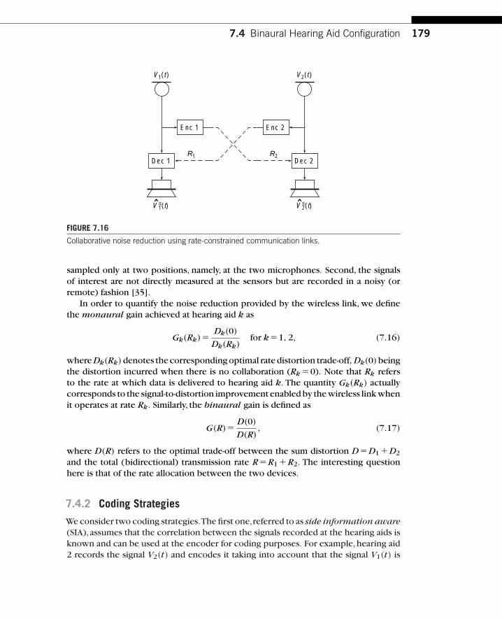
7.4 Binaural Hearing Aid Configuration 179
Enc 1
Dec 1
V s1(t)
Dec 2
Enc 2
V1(t)
R1 R2
V2(t)
ˆ V s2(t)ˆ
FIGURE 7.16
Collaborative noise reduction using rate-constrained communication links.
sampled only at two positions, namely, at the two microphones. Second, the signalsof interest are not directly measured at the sensors but are recorded in a noisy (orremote) fashion [35].
In order to quantify the noise reduction provided by the wireless link, we definethe monaural gain achieved at hearing aid k as
Gk(Rk)�Dk(0)
Dk(Rk)for k�1, 2, (7.16)
where Dk(Rk) denotes the corresponding optimal rate distortion trade-off, Dk(0) beingthe distortion incurred when there is no collaboration (Rk �0). Note that Rk refersto the rate at which data is delivered to hearing aid k. The quantity Gk(Rk) actuallycorresponds to the signal-to-distortion improvement enabled by the wireless link whenit operates at rate Rk. Similarly, the binaural gain is defined as
G(R)�D(0)
D(R), (7.17)
where D(R) refers to the optimal trade-off between the sum distortion D �D1 �D2
and the total (bidirectional) transmission rate R�R1 �R2. The interesting questionhere is that of the rate allocation between the two devices.
7.4.2 Coding Strategies
We consider two coding strategies.The first one,referred to as side information aware(SIA), assumes that the correlation between the signals recorded at the hearing aids isknown and can be used at the encoder for coding purposes. For example,hearing aid2 records the signal V2(t) and encodes it taking into account that the signal V1(t) is

180 CHAPTER 7 Distributed Compression in Microphone Arrays
(a)
Dec 1Enc 2R1
V1(t)
V2(t)
(b)
Dec 1Dec 0V
s2(t )
V
s1(t )
Enc 2R1
V1(t)
V2(t)
V s1(t )
V s1(t )
FIGURE 7.17
The two coding strategies considered for the binaural hearing aid configuration. (a) Sideinformation aware coding. (b) Side information unaware coding.
available at the decoder, that is, at hearing aid 1. This coding scheme is schematicallyrepresented in Figure 7.17(a).The second class of coding methods, referred to as sideinformation unaware (SIU), does not assume that such statistics can be computedat the encoder. In this case, hearing aid 2 encodes its observation V2(t) for a decoder(Dec 0) that does not have access to the side information V1(t). The transmitted datais decoded and subsequently used together with V1(t) in a second decoder (Dec 1) toestimate the desired speech component V s
1 (t). This is depicted in Figure 7.17(b). Ina practical setting, the statistics of the speech and noise components can be typicallylearned at the decoder by means of a voice activity detection mechanism [38]. Notealso that, as the statistics between the signals recorded at the two hearing devices arenot known at the encoder, this latter assumes that the process to be estimated at theother end is V s
2 (t) and optimizes its coding strategy accordingly.
7.4.3 Rate-distortion Trade-offs
We first study a simple acoustic environment that allows us to derive optimalrate-distortion trade-offs and rate-allocation policies in closed form. Though clearlysimplistic, the considered assumptions preserve many of the features observed ina realistic scenario, in particular for the rate-allocation problem, as observed in thesequel.
We consider a single speech source surrounded by ambient noise. The recordedsignals (7.15) can be expressed as
Vk(t)�S(t)∗hk(t)�Nk(t) for k�1, 2,
where S(t) denotes the source,hk(t) the acoustic impulse response from the source tomicrophone k,and Nk(t) uncorrelated Gaussian noise signals.The desired component

7.4 Binaural Hearing Aid Configuration 181
at hearing aid k is thus V sk(t)�S(t)∗hk(t). We assume omnidirectional microphones,
neglect the head-shadow effect (see Section 7.2.1.4) and work under the far-fieldassumption. In this case,hk(t) reduces to a simple delay proportional to the distancedk between the source and the microphone, that is,
hk(t)��(t �dk/c).
We further assume that the speech and noise sources have flat power spectral den-sities with maximal frequency �0. The variance of the source is �2
S , and the SNR atmicrophone k is denoted �k. With these restrictions, the optimal rate-distortion trade-off at hearing aid 1 with the SIA coding scheme, denoted D1,a(R), can be expressedas [39]
D1,a(R1)��0
�
�2S �1�2
1��1 ��2
(1�
�2
1��12
�2�R1
�0
)for R1 �0. (7.18)
Similarly, the optimal rate-distortion trade-off obtained with the SIU coding scheme,denoted D1,u(R), is given by
D1,u(R1)��0�2
S
��1
(1�
1��2
�1
(1��2 2
�2�R1
�0
)�1)�1
for R1 �0. (7.19)
We observe that, in this scenario, the results depend neither on the position of thesource nor on the geometrical properties of the binaural hearing aid configuration.This results from the far-field assumption and the fact that the noise is uncorrelatedacross microphones. From a more practical point of view, it can be shown [39] thatan optimal encoding architecture with the SIA coding scheme can be broken intotwo stages. Call V2(t) the minimum MSE estimate of V2(t) given V1(t). An optimalstrategy amounts to (i) filtering V2(t) by the Wiener filter designed to estimate V s
1 (t)using V2(t) and (ii) encoding this estimate optimally, taking into account the sideinformation V1(t) available at the decoder. Knowledge of the statistics between V1(t)and V2(t) is thus required at the encoder. Similarly, an optimal encoding architec-ture with the SIU strategy amounts to (i) computing the minimum MSE estimate ofV s
2 (t) using V2(t) and (ii) encoding this estimate optimally for a decoder that doesnot have access to the side information V1(t). In this case, however, the requiredstatistics can be computed at the encoder by means of a voice activity detectionmechanism [38].
To get some insights into the gain provided by the wireless link as a function ofthe communication bit rate, let us consider the case of equal SNRs (�1 ��2 ��). InFigure 7.18,we plot the monaural gain rate function (7.16) corresponding to the twocoding schemes for different values of �. At 10 dB (see Figure 7.18(a)), we observethat the SIU coding strategy may lead to a significant loss in terms of noise reductioncapability in comparison to the SIA scheme. However, as the input SNR decreases(see Figures 7.18(b) and 7.18(c)), the spatial correlation between the recorded signalsdecreases significantly and the gap between the SIA and SIU curves vanishes for all

182 CHAPTER 7 Distributed Compression in Microphone Arrays
0
0.2
0.4
0.6
0.8
1
1.2
1.4
1.6
1.8
0 10 20 30 40 50 60 70Rate (kb/s)
(c)
Gai
n (d
B)
SIA CodingSIU Coding
SIA CodingSIU Coding
0 10 20 30 40 50 60 700
0.5
1
1.5
2
2.5
3
Rate (kb/s)
Gai
n (d
B)
0
0.5
1
1.5
2
2.5
3
Gai
n (d
B)
0 10 20 30 40 50 60 70Rate (kb/s)
(a) (b)
SIA CodingSIU Coding
FIGURE 7.18
Monaural gain rate functions for different input signal-to-noise ratios � and a maximum frequencyf0 ��0/(2�)�5 kHz. (a) � �20 dB. (b) � �10 dB. (c) � �0 dB. We observe that the gainachieved by taking the side information into account may be significant at high SNR but vanishesin very noisy scenarios.
rates. The result suggests that the use of SIA coding strategies is uninteresting in verynoisy scenarios.
Let us now turn our attention to the general binaural system depicted in Figure 7.16.Without loss of generality,we assume that �1 ��2.A natural question that arises in thiscontext is that of the optimal rate allocation between the two hearing instruments.More precisely, if you assume that you are given a total bit budget of R bits per second,how should this be allocated to R1 and R2 to minimize the sum distortion D �D1 �D2,hence maximizing the binaural gain G(R) given by (7.17)? Under the acoustic modelwe have considered, the optimal rate-allocation strategy for the SIA coding scheme
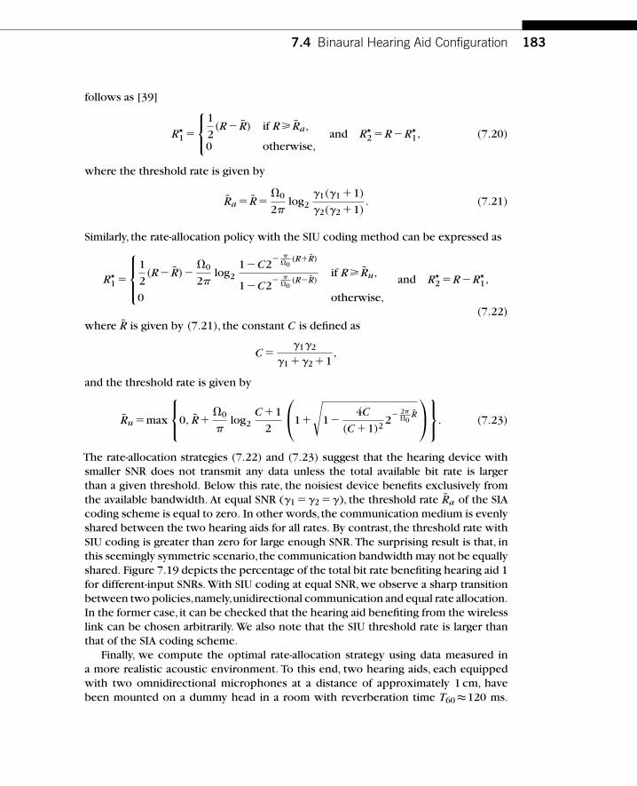
7.4 Binaural Hearing Aid Configuration 183
follows as [39]
R�1 �
⎧⎨⎩1
2(R� R) if R� Ra,
0 otherwise,and R�
2 �R�R�1, (7.20)
where the threshold rate is given by
Ra � R��0
2�log2
�1(�1 �1)
�2(�2 �1). (7.21)
Similarly, the rate-allocation policy with the SIU coding method can be expressed as
R�1 �
⎧⎪⎨⎪⎩1
2(R� R)�
�0
2�log2
1�C2� �
�0(R�R)
1�C2� �
�0(R�R)
if R� Ru,
0 otherwise,
and R�2 �R�R�
1,
(7.22)
where R is given by (7.21), the constant C is defined as
C ��1�2
�1 ��2 �1,
and the threshold rate is given by
Ru �max
⎧⎨⎩0, R��0
�log2
C �1
2
⎛⎝1�
√1�
4C
(C �1)22
� 2��0
R
⎞⎠⎫⎬⎭. (7.23)
The rate-allocation strategies (7.22) and (7.23) suggest that the hearing device withsmaller SNR does not transmit any data unless the total available bit rate is largerthan a given threshold. Below this rate, the noisiest device benefits exclusively fromthe available bandwidth. At equal SNR (�1 ��2 ��), the threshold rate Ra of the SIAcoding scheme is equal to zero. In other words, the communication medium is evenlyshared between the two hearing aids for all rates. By contrast, the threshold rate withSIU coding is greater than zero for large enough SNR. The surprising result is that, inthis seemingly symmetric scenario,the communication bandwidth may not be equallyshared. Figure 7.19 depicts the percentage of the total bit rate benefiting hearing aid 1for different-input SNRs. With SIU coding at equal SNR, we observe a sharp transitionbetween two policies,namely,unidirectional communication and equal rate allocation.In the former case, it can be checked that the hearing aid benefiting from the wirelesslink can be chosen arbitrarily. We also note that the SIU threshold rate is larger thanthat of the SIA coding scheme.
Finally, we compute the optimal rate-allocation strategy using data measured ina more realistic acoustic environment. To this end, two hearing aids, each equippedwith two omnidirectional microphones at a distance of approximately 1 cm, havebeen mounted on a dummy head in a room with reverberation time T60 ≈120 ms.

184 CHAPTER 7 Distributed Compression in Microphone Arrays
0 50 100 150 200 250 300Total rate (kb/s)
0
5
10
15
20
25
30
35
40
45
50
55
Rat
e al
loca
tion
(%)
(10, 10)
(20, 10)
(30, 10)
(40, 10)
SIA CodingSIU Coding
FIGURE 7.19
Percentage of the total bit rate benefiting hearing aid 1. The maximum frequency isf0 � �0/(2�) � 5 kHz, and the different sets of curves correspond to various SNR pairs(�1, �2). We observe that the threshold rate for SIU coding is larger than that of SIA coding.
The acoustic transfer functions for the four microphones have been measured every15◦ in the horizontal plane for a loudspeaker at a distance of 1 m. Here, the anglesare measured clockwise, and the zero angle corresponds to the front. The samplingfrequency is set to 20.48 kHz. The acoustic scene is synthesized using the measuredtransfer functions.The speech component in (7.15) is a single speech source at 0◦.Thenoise component consists of a stationary white Gaussian ambient noise along with aninterfering point source at 90◦.The power spectral density of the speech component isestimated using 3 seconds of a sentence of the HINT database [40].The power spectraldensity of the interferer is computed using a 3-second segment of multitalker babblenoise available in the NOISEX-92 database [41]. The power of the involved sources isadjusted so as to meet a desired SNR and interference-to-noise ratio of 10 dB at thefront microphone of hearing aid 1 that is, the signal-to-interference ratio is equal to0 dB.The optimal rate allocation is obtained numerically and is plotted in Figure 7.20.Here,we only consider the front microphone of each hearing aid. Since the interferingpoint source is located on the right-hand side of the head, the SNR of hearing aid 1is higher owing to the head-shadow effect. Up to a threshold bit rate, hearing aid 2

7.5 Conclusions 185
0 0.1 0.2 0.3 0.4 0.5 0.6Rate (kb/s)
0
5
10
15
20
25
30
35
40
45
50R
ate
allo
catio
n (%
)
SIA CodingSIU Coding
FIGURE 7.20
Percentage of the total bit rate benefiting hearing aid 1 in the presence of an interfering pointsource at 90◦. Hearing aid 2 has the smallest SNR and thus benefits exclusively from thecommunication bandwidth up to a threshold rate that depends on the chosen coding strategy.
thus benefits exclusively from the available communication bandwidth. In this case,the fraction allocated to hearing aid 1 is zero. We observe that this threshold is higherwith the SIU coding scheme,corroborating the analytical results obtained in the simplescenario considered previously.
7.5 CONCLUSIONSThe problem of distributed compression has been studied for the specific case ofmicrophone arrays.A large portion of the exposition has been devoted to the study ofthe spatiotemporal characteristics of the sound field. In particular, it has been shownthat the spatiotemporal impulse response is almost bandlimited to a region that hasa butterfly shape. The insights gained from this analysis have been subsequently usedfor two distributed coding setups of practical interest. The first one has consideredthe gathering of audio signals recorded by remote sensors at a base station. It has been

186 CHAPTER 7 Distributed Compression in Microphone Arrays
shown that, under simplifying assumptions, judicious signal processing at the sensorscan achieve the best rate-distortion trade-off.We have thus provided the solution to themultiterminal source coding problem for this particular scenario. The second setuphas involved two digital hearing aids allowed to exchange audio signals using a wirelesscommunication medium as a way to provide collaborative noise reduction. Optimalgain rate trade-offs have been derived,and optimal rate-allocation strategies have beendiscussed.
ACKNOWLEDGMENTThis work was supported by the National Competence Center in Research onMobile Information and Communication Systems (NCCR-MICS,http://www.mics.org),a center supported by the Swiss National Science Foundation under grant number5005-67322.
REFERENCES[1] G. Barrenetxea, F. Ingelrest, G. Schaefer, M. Vetterli, O. Couach, and M. Parlange, “Sensor-
Scope: Out-of-the-box environmental monitoring,” ACM/IEEE International Conference onInformation Processing in Sensor Networks, pp. 332–343, April 2008.
[2] D. Li,K.Wong, Y. Hu,andA. Sayeed,“Detection,classification,tracking of targets in micro-sensornetworks,” IEEE Signal Processing Mag., vol. 19, no. 2, pp. 17–29, March 2002.
[3] J. C. Chen, K. Yao, and R. E. Hudson, “Source localization and beamforming,” IEEE SignalProcessing Mag., vol. 19, no. 2, pp. 30–39, March 2002.
[4] B. Beferull-Lozano, R. L. Konsbruck, and M. Vetterli,“Rate-distortion problem for physics baseddistributed sensing,” ACM/IEEE International Conference on Information Processing inSensor Networks, pp. 330–339, April 2004.
[5] J. Breebaart and C. Faller, Spatial Audio Processing. Wiley, 2007.
[6] D. T. Yang, C. Kyriakakis, and C.-C. J. Kuo, High-Fidelity Multichannel Audio Coding, ser.EURASIP Book Series on Signal Processing and Communications. Hindawi Publishing, 2004,vol. 1.
[7] S. S. Pradhan and K. Ramchandran, “Distributed source coding using syndromes (DISCUS):Design and construction,” IEEE Trans. Inform.Theory, vol. 49,no. 3,pp. 626–634,March 2003.
[8] A. Majumdar,K. Ramchandran,and I. Kozintsev,“Distributed coding for wireless audio sensors,”IEEE Workshop on Applications of Signal Processing to Audio and Acoustics, pp. 209–212,October 2003.
[9] H. Dong, J. Lu, and Y. Sun, “Distributed audio coding in wireless sensor networks,” IEEEInternational Conference on Computational Intelligence and Security, vol. 2, no. 1, pp.1695–1699, November 2006.
[10] O. Roy and M.Vetterli,“Distributed spatial audio coding in wireless hearing aids,”IEEE Workshopon Applications of Signal Processing to Audio and Acoustics, pp. 227–230, October 2007.
[11] P. M. Morse and K. U. Ingard,Theoretical Acoustics. McGraw-Hill, 1968.
[12] P. S. Naidu, Sensor Array Signal Processing. CRC Press, 2001.

References 187
[13] D. H. Johnson and D. E. Dudgeon, Array Signal Processing: Concepts andTechniques. Prentice-Hall, 1993.
[14] T. Adjler, L. Sbaiz, and M. Vetterli, “Dynamic measurement of room impulse responses usinga moving microphone,” The Journal of the Acoustical Society of America, vol. 122, no. 3,pp. 1636–1645, September 2007.
[15] J. B. Allen and D. A. Berkley,“Image method for efficiently simulating small-room acoustics,”TheJournal of the Acoustical Society of America, vol. 65, pp. 943–950, 1979.
[16] H. Moller,“Fundamentals of binaural technology,”Appl. Acoust., vol. 36, pp. 171–218, 1992.
[17] R. O. Duda andW. Martens,“Range dependence of the response of a spherical head model,”TheJournal of the Acoustical Society of America, vol. 104, pp. 3048–3058, 1998.
[18] T. Ajdler, L. Sbaiz, and M. Vetterli, “The plenacoustic function and its sampling,” IEEE Trans.Signal Processing, vol. 54, no. 10, pp. 3790–3804, 2006.
[19] E. G. Williams, Fourier Acoustics. Academic Press, 1999.
[20] M. Vetterli and J. Kovacevic, Wavelets and Subband Coding. Prentice Hall, 1995. [Online].Available: http://www.waveletsandsubbandcoding.org.
[21] P. Vaidyanathan, Multirate Systems and Filter Banks. Prentice Hall, 1992.
[22] F. Bureau,“Le traité de la lumière de Christian Huygens,”Acad.Roy.Belgique.Bull.Cl.Sci.,vol. 32,pp. 730–744, January 1946.
[23] A. J. Berkhout, D. de Vries, and P. Vogel, “Acoustic control by wave field synthesis,” TheJournal of the Acoustical Society of America, vol. 93, no. 5, p. 2764–2778, May 1993.
[24] E. Wong and B. Hajek, Stochastic Processes in Engineering Systems. Springer-Verlag, 1985.
[25] T. Berger, Rate Distortion Theory: A Mathematical Basis for Data Compression. Prentice-Hall,1971.
[26] T. M. Cover and J. A. Thomas, Elements of Information Theory. Wiley, 1991.
[27] R. L. Konsbruck, E. Telatar, and M. Vetterli,“On the multiterminal rate distortion function foracoustic sensing,” submitted to IEEE Trans. Inform.Theory, January 2008.
[28] V. Goyal,“Theoretical foundations of transform coding,” IEEE Signal Processing Mag., vol. 18,pp. 9–21, September 2001.
[29] M. Gastpar, P. L. Dragotti, and M. Vetterli, “The distributed Karhunen–Loève transform,” IEEETrans. Inform.Theory, no. 12, pp. 5177–5196, December 2006.
[30] T. Flynn and R. Gray,“Encoding of correlated observations,”IEEE Trans. Inform.Theory, vol. 33,no. 6, pp. 773–787, November 1987.
[31] H. Yamamoto and K. Itoh, “Source coding theory for multiterminal communication systemswith a remote source,”Trans. IECE Japan, vol. E63, no. 10, pp. 700–706, October 1980.
[32] S. C. Draper,“Successive structuring of source coding algorithms for data fusion,buffering anddistribution in networks,”Ph.D. dissertation,Massachusetts Institute of Technology, June 2002.
[33] H. S.Witsenhausen,“Indirect rate-distortion problem,”IEEE Trans.Inform. Theory,vol. 26,no. 5,pp. 518–521, September 1980.
[34] R. L. Dobrushin and B. S.Tsybakov, “Information transmission with additional noise,”IEEETrans.Inform.Theory, vol. 8, no. 5, pp. 293–304, September 1962.
[35] D. J. Sakrison,“Source encoding in the presence of random disturbance,” IEEE Trans. Inform.Theory, vol. 14, no. 1, pp. 165–167, January 1968.
[36] J. K. Wolf and J. Ziv, “Transmission of noisy information to a noisy receiver with minimumdistortion,” IEEE Trans. Inform.Theory, vol. 16, no. 4, pp. 406–411, July 1970.
[37] D. Rebollo-Monedero, S. Rane, A. Aaron, and B. Girod, “High-rate quantization and transformcoding with side information at the decoder,”EURASIP Journal on Signal Processing, SpecialIssue on Distributed Source Coding, vol. 86, no. 11, pp. 3160–3179, 2006.

188 CHAPTER 7 Distributed Compression in Microphone Arrays
[38] L. R. Rabiner and R. W. Schafer, Digital Processing of Speech Signals. Prentice-Hall, 1978.
[39] O. Roy and M.Vetterli,“Rate-constrained collaborative noise reduction for wireless hearing aids,”to appear in IEEE Trans. Signal Processing, 2009.
[40] M. Nilsson, S. D. Soli, and A. Sullivan,“Development of the Hearing in Noise Test for the mea-surement of speech reception thresholds in quiet and in noise,”The Journal of the AcousticalSociety of America, vol. 95, no. 2, pp. 1085–1099, 1994.
[41] A. Varga,H. Steeneken,M.Tomlinson,and D. Jones,“The NOISEX-92 study on the effect of addi-tive noise on automatic speech recognition,” Speech Research Unit, Defense Research Agency,Malvern, U.K.,Tech. Rep., 1992.
CHAPTER
8Distributed Video Coding:Basics, Codecs, andPerformance
Fernando Pereira, Catarina Brites, and Joao AscensoInstituto Superior Técnico—Instituto de Telecomunicações, 1049-001 Lisbon, Portugal
C H A P T E R C O N T E N T SIntroduction . . . . . . . . . . . . . . . . . . . . . . . . . . . . . . . . . . . . . . . . . . . . . . . . . . . . . . . . . . . . . . . . . . . . . . . . . . . . . . 190Basics on Distributed Video Coding . . . . . . . . . . . . . . . . . . . . . . . . . . . . . . . . . . . . . . . . . . . . . . . . . . . . . . 192The Early Wyner–Ziv Video Coding Architectures . . . . . . . . . . . . . . . . . . . . . . . . . . . . . . . . . . . . . . . . 195
The Stanford WZ Video Codec . . . . . . . . . . . . . . . . . . . . . . . . . . . . . . . . . . . . . . . . . . . . . . . . . . . . . 195The Berkeley WZ Video Codec . . . . . . . . . . . . . . . . . . . . . . . . . . . . . . . . . . . . . . . . . . . . . . . . . . . . . 198Comparing the Early WZ Video Codecs . . . . . . . . . . . . . . . . . . . . . . . . . . . . . . . . . . . . . . . . . . . . . 200
Further Developments on Wyner–Ziv Video Coding. . . . . . . . . . . . . . . . . . . . . . . . . . . . . . . . . . . . . . . 201Improving RD Performance . . . . . . . . . . . . . . . . . . . . . . . . . . . . . . . . . . . . . . . . . . . . . . . . . . . . . . . . 201Removing the Feedback Channel . . . . . . . . . . . . . . . . . . . . . . . . . . . . . . . . . . . . . . . . . . . . . . . . . . 204Improving Error Resilience . . . . . . . . . . . . . . . . . . . . . . . . . . . . . . . . . . . . . . . . . . . . . . . . . . . . . . . . . 205Providing Scalability . . . . . . . . . . . . . . . . . . . . . . . . . . . . . . . . . . . . . . . . . . . . . . . . . . . . . . . . . . . . . . . 206
The DISCOVER Wyner–Ziv Video Codec . . . . . . . . . . . . . . . . . . . . . . . . . . . . . . . . . . . . . . . . . . . . . . . . . . 207Transform and Quantization . . . . . . . . . . . . . . . . . . . . . . . . . . . . . . . . . . . . . . . . . . . . . . . . . . . . . . . . 210Slepian–Wolf Coding . . . . . . . . . . . . . . . . . . . . . . . . . . . . . . . . . . . . . . . . . . . . . . . . . . . . . . . . . . . . . . . 211Side Information Creation . . . . . . . . . . . . . . . . . . . . . . . . . . . . . . . . . . . . . . . . . . . . . . . . . . . . . . . . . . 213Correlation Noise Modeling . . . . . . . . . . . . . . . . . . . . . . . . . . . . . . . . . . . . . . . . . . . . . . . . . . . . . . . . 214Reconstruction . . . . . . . . . . . . . . . . . . . . . . . . . . . . . . . . . . . . . . . . . . . . . . . . . . . . . . . . . . . . . . . . . . . . . 215
The DISCOVER Codec Performance . . . . . . . . . . . . . . . . . . . . . . . . . . . . . . . . . . . . . . . . . . . . . . . . . . . . . 216Performance Evaluation Conditions . . . . . . . . . . . . . . . . . . . . . . . . . . . . . . . . . . . . . . . . . . . . . . . . 216RD Performance Evaluation . . . . . . . . . . . . . . . . . . . . . . . . . . . . . . . . . . . . . . . . . . . . . . . . . . . . . . . . 219Complexity Performance Evaluation. . . . . . . . . . . . . . . . . . . . . . . . . . . . . . . . . . . . . . . . . . . . . . . . 232
Final Remarks . . . . . . . . . . . . . . . . . . . . . . . . . . . . . . . . . . . . . . . . . . . . . . . . . . . . . . . . . . . . . . . . . . . . . . . . . . . 241Acknowledgments . . . . . . . . . . . . . . . . . . . . . . . . . . . . . . . . . . . . . . . . . . . . . . . . . . . . . . . . . . . . . . . . . . . . . . . . 242References . . . . . . . . . . . . . . . . . . . . . . . . . . . . . . . . . . . . . . . . . . . . . . . . . . . . . . . . . . . . . . . . . . . . . . . . . . . . . . . 242
Distributed Source Coding: Theory, Algorithms, and ApplicationsCopyright © 2008 by Academic Press, Inc. All rights of reproduction in any form reserved. 189
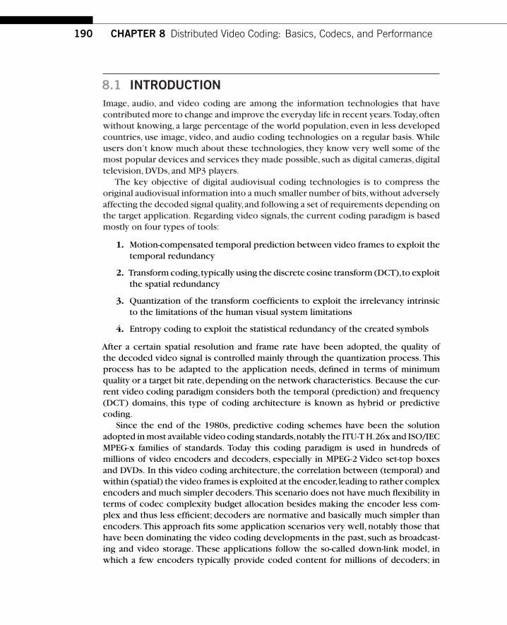
190 CHAPTER 8 Distributed Video Coding: Basics, Codecs, and Performance
8.1 INTRODUCTIONImage, audio, and video coding are among the information technologies that havecontributed more to change and improve the everyday life in recent years.Today,oftenwithout knowing, a large percentage of the world population, even in less developedcountries, use image, video, and audio coding technologies on a regular basis. Whileusers don’t know much about these technologies, they know very well some of themost popular devices and services they made possible, such as digital cameras,digitaltelevision, DVDs, and MP3 players.
The key objective of digital audiovisual coding technologies is to compress theoriginal audiovisual information into a much smaller number of bits,without adverselyaffecting the decoded signal quality,and following a set of requirements depending onthe target application. Regarding video signals, the current coding paradigm is basedmostly on four types of tools:
1. Motion-compensated temporal prediction between video frames to exploit thetemporal redundancy
2. Transform coding,typically using the discrete cosine transform (DCT),to exploitthe spatial redundancy
3. Quantization of the transform coefficients to exploit the irrelevancy intrinsicto the limitations of the human visual system limitations
4. Entropy coding to exploit the statistical redundancy of the created symbols
After a certain spatial resolution and frame rate have been adopted, the quality ofthe decoded video signal is controlled mainly through the quantization process. Thisprocess has to be adapted to the application needs, defined in terms of minimumquality or a target bit rate,depending on the network characteristics. Because the cur-rent video coding paradigm considers both the temporal (prediction) and frequency(DCT) domains, this type of coding architecture is known as hybrid or predictivecoding.
Since the end of the 1980s, predictive coding schemes have been the solutionadopted in most available video coding standards,notably the ITU-T H.26x and ISO/IECMPEG-x families of standards. Today this coding paradigm is used in hundreds ofmillions of video encoders and decoders, especially in MPEG-2 Video set-top boxesand DVDs. In this video coding architecture, the correlation between (temporal) andwithin (spatial) the video frames is exploited at the encoder,leading to rather complexencoders and much simpler decoders.This scenario does not have much flexibility interms of codec complexity budget allocation besides making the encoder less com-plex and thus less efficient; decoders are normative and basically much simpler thanencoders. This approach fits some application scenarios very well, notably those thathave been dominating the video coding developments in the past, such as broadcast-ing and video storage. These applications follow the so-called down-link model, inwhich a few encoders typically provide coded content for millions of decoders; in

8.1 Introduction 191
this case, the decoder complexity is the critical issue and thus has to be minimized.Moreover,the temporal prediction loop used to compute the residues to transmit,afterthe motion-compensated prediction of the current frame,requires the decoder to runthe same loop in perfect synchronization with the encoder. This means that, whenchannel errors are present, errors may propagate in time, strongly affecting the videoquality, typically until some (Intra) coding refreshment is performed.
The H.264/AVC (Advanced Video Coding) standard is the most efficient video cod-ing standard available [1], typically spending about 50 percent of the rate for the samequality regarding previous video coding standards. It is being adopted for a wide rangeof applications from mobile videotelephony to HDTV and Blu-ray discs. Besides thetechnical novelty adopted in this standard (e.g.,in terms of motion estimation and com-pensation, spatial transform, and entropy coding), the compression gains very muchrely on additional significant encoder and decoder complexity.To provide coding solu-tions adapted to a wide range of applications, the standard defines a set of profiles andlevels [1],which constrain the very flexible coding syntax in appropriate ways to allowsuccessful deployment. Meanwhile, some of the most relevant compression gains arecoming from control of the H.264/AVC codec through adequate encoder tools since,as usual,H.264/AVC encoders are not normative,thus leaving space for improvementsin rate-distortion (RD) performance while still guaranteeing the same compatibilitywith much simpler decoders.
With the recent wide deployment of wireless networks,a growing number of appli-cations do not fit well the typical down-link model but rather follow an up-link modelin which many senders deliver data to a central receiver. Examples of these appli-cations are wireless digital video cameras, low-power video sensor networks, andsurveillance systems. Typically, these emerging applications require light encoding ora flexible distribution of the codec complexity, robustness to packet losses,high com-pression efficiency,and,often, low latency/delay as well.There is also a growing use ofmultiview video content, which means the data to be delivered regards many (corre-lated) views of the same scene. In many cases, to keep the sensing system simple, theassociated cameras cannot communicate among themselves, preventing the usage ofa predictive approach to exploit the interview redundancy.
In terms of video coding, these emerging applications are asking for a novel videocoding paradigm that is better adapted to the specific characteristics of the new sce-narios. Ideally, these applications would welcome a new video coding paradigm ableto address all the requirements above with the same coding efficiency as the bestpredictive coding schemes available, as well as with an encoder complexity and errorrobustness similar to the current best Intra coding solutions, which are the simplestand most error-robust solutions.
To address these needs, around 2002, some research groups decided to revisit thevideo coding problem in light of two information theory results from the 1970s: theSlepian–Wolf theorem [2] and the Wyner–Ziv theorem [3]. These efforts gave birth towhat is now known as distributed video coding (DVC), and Wyner–Ziv (WZ) videocoding,as a particular case of distributed video coding.This chapter presents the devel-opments that have been produced in DVC following the early research initiatives.

192 CHAPTER 8 Distributed Video Coding: Basics, Codecs, and Performance
To achieve this purpose, this chapter is organized as follows: building on previouschapters, Section 8.2 will briefly review the basic concepts and theorems underpin-ning DVC. Next, Section 8.3 will present the first distributed video codecs developed,while Section 8.4 will review some of the most relevant developments following theearly DVC codecs. To get a more precise understanding of how a DVC codec works,Section 8.5 will present in detail perhaps the most efficient DVC codec available, theDISCOVER WZ video codec [4, 5]. Section 8.6 will propose a detailed performanceevaluation of the DISCOVER WZ codec, which may be used as benchmarking. Finally,Section 8.7 will summarize the past developments and project the future in the DVCarena.
8.2 BASICS ON DISTRIBUTED VIDEO CODINGAs mentioned in a previous chapter, the Slepian–Wolf theorem addresses the casewhere two statistically dependent discrete random sequences, independently andidentically distributed (i.i.d.), X and Y , are independently encoded, and thus notjointly encoded as in the largely deployed predictive coding solution. The Slepian–Wolf theorem states that the minimum rate to encode the two (correlated) sourcesis the same as the minimum rate for joint encoding, with an arbitrarily small errorprobability. This distributed source coding (DSC) paradigm is an important resultin the context of the emerging application challenges presented earlier, since itopens the doors to new coding solutions where, at least in theory, separate encodingand joint decoding does not induce any compression efficiency loss when com-pared to the joint encoding and decoding used in the traditional predictive codingparadigm. In theory, the rate bounds for a vanishing error probability considering twosources are
RX �H(X |Y )
RY �H(Y |X) (8.1)
(RX �RY )�H(X, Y ),
which corresponds to the area identified in Figure 8.1. This basically means that theminimum coding rate is the same as for joint encoding (i.e.,the joint entropy),providedthat the individual rates for both sources are higher than the respective conditionalentropies.
Slepian–Wolf coding is the term generally used to characterize lossless codingarchitectures that follow this independent encoding approach. Slepian–Wolf codingis also referred to in the literature as lossless distributed source coding since it con-siders that the two statistically dependent sequences are perfectly reconstructed ata joint decoder (neglecting the arbitrarily small probability of decoding error), thusapproaching the lossless case.
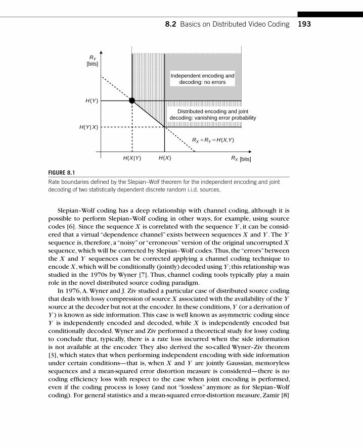
8.2 Basics on Distributed Video Coding 193
Independent encoding anddecoding: no errors
Distributed encoding and jointdecoding: vanishing error probability
RX 1RY 5H (X,Y )
RX [bits]
RY[bits]
H (X )
H (Y )
H(X |Y )
H(Y | X )
FIGURE 8.1
Rate boundaries defined by the Slepian–Wolf theorem for the independent encoding and jointdecoding of two statistically dependent discrete random i.i.d. sources.
Slepian–Wolf coding has a deep relationship with channel coding, although it ispossible to perform Slepian–Wolf coding in other ways, for example, using sourcecodes [6]. Since the sequence X is correlated with the sequence Y , it can be consid-ered that a virtual “dependence channel” exists between sequences X and Y . The Ysequence is, therefore, a “noisy” or “erroneous” version of the original uncorrupted Xsequence,which will be corrected by Slepian–Wolf codes.Thus, the“errors”betweenthe X and Y sequences can be corrected applying a channel coding technique toencode X ,which will be conditionally (jointly) decoded using Y ; this relationship wasstudied in the 1970s by Wyner [7]. Thus, channel coding tools typically play a mainrole in the novel distributed source coding paradigm.
In 1976, A. Wyner and J. Ziv studied a particular case of distributed source codingthat deals with lossy compression of source X associated with the availability of the Ysource at the decoder but not at the encoder. In these conditions,Y (or a derivation ofY ) is known as side information.This case is well known as asymmetric coding sinceY is independently encoded and decoded, while X is independently encoded butconditionally decoded. Wyner and Ziv performed a theoretical study for lossy codingto conclude that, typically, there is a rate loss incurred when the side informationis not available at the encoder. They also derived the so-called Wyner–Ziv theorem[3], which states that when performing independent encoding with side informationunder certain conditions—that is, when X and Y are jointly Gaussian, memorylesssequences and a mean-squared error distortion measure is considered—there is nocoding efficiency loss with respect to the case when joint encoding is performed,even if the coding process is lossy (and not “lossless” anymore as for Slepian–Wolfcoding). For general statistics and a mean-squared error-distortion measure, Zamir [8]

194 CHAPTER 8 Distributed Video Coding: Basics, Codecs, and Performance
also proved that the rate loss is less than 0.5 bit/sample. Later, it was shown that,for norate loss,only the innovation,this means the X �Y difference needs to be Gaussian [9].
Together,the Slepian–Wolf and theWyner–Ziv theorems suggest that it is possible tocompress two statistically dependent signals in a distributed way (separate encoding,joint decoding), approaching the coding efficiency of conventional predictive codingschemes (joint encoding and decoding). Based on these theorems, a new videocoding paradigm, well known as distributed video coding, has emerged havingWyner–Ziv coding as its lossy particular case.
DVC does not rely on joint encoding, and thus, when applied to video coding,it typically results in the absence of the temporal prediction loop (always used inpredictive schemes) and lower complexity encoders. DVC-based architectures mayprovide the following functional benefits, which are important for many emergingapplications:
1. Flexible allocation of the global video codec complexity
2. Improved error resilience
3. Codec independent scalability (since upper layers do not have to rely on preciselower layers)
4. Exploitation of multiview correlation without cameras/encoders communicat-ing among them
These functional benefits can be relevant for a large range of emerging applicationscenarios such as wireless video cameras, low-power surveillance,video conferencingwith mobile devices, disposable video cameras, visual sensor networks, distributedvideo streaming,multiview video systems,and wireless capsule endoscopy [10].Whilethis chapter will concentrate on monoview video coding, multiview video codingusing a DVC approach is also a very hot research topic;check [11] for a review on thissubject.
Practical design of WZ video codecs started around 2002, following importantadvances in channel coding technology,especially error-correction codes with a capac-ity close to the Shannon limit, for example,turbo and low-density parity-check (LDPC)codes. While theory suggests that DVC solutions may be as efficient as joint encodingsolutions, practical developments did not yet achieve that performance for all typesof content,especially if low-complexity encoding is also targeted. Part of this gap maybe filled with more research to make the technology more mature, but there are alsosome practical limitations that may be difficult to overcome. For example, while thetheory assumes that the encoder knows the statistical correlation between the twosources, X and Y , and that the innovation X �Y is Gaussian, in practical conditionsthis is often not true. Naturally, the better the encoder knows the statistical correla-tion between X and Y , the higher the compression efficiency. This highlights a mainDVC coding paradox: although encoders may be rather simple, they may also need tobecome more complex to increase the compression efficiency and reach the limitsset by the theory. This is one of the DVC research challenges being faced today.

8.3 The Early Wyner–Ziv Video Coding Architectures 195
8.3 THE EARLY WYNER–ZIV VIDEO CODINGARCHITECTURES
The first practical WZ video coding solutions emerged around 2002, notably fromStanford University [12–14] and the University of California (UC), Berkeley [15, 16].The Stanford architecture is mainly characterized by frame-based Slepian–Wolf coding,typically using turbo codes, and a feedback channel to perform rate control at thedecoder;the BerkeleyWZ video coding solution is mainly characterized by block-basedcoding with decoder motion estimation.
The Stanford architecture was later adopted and improved by many research groupsaround the world. However,while there are many papers published with changes andimprovements to this architecture, the precise and detailed evaluation of its perfor-mance, targeting its deep understanding for later advances, was not presented untilrecently. Available performance results were mostly partial (e.g., typically only fewRD performance results), under unclear and incompatible conditions (e.g., differentsequences, different sets of frames for each sequence, different key frames coding),using vaguely defined and also sometimes architecturally unrealistic codecs (e.g.,assuming the original frames available at the decoder), using side information at theencoder, or a vague side information creation process. This chapter will present anextensive performance evaluation of one of the most representative (and best per-forming) DVC codecs, the DISCOVER WZ codec. However, considering the impactthey had in the DVC research arena, first this section will review and compare theearly Stanford and Berkeley Wyner–Ziv video coding solutions.
8.3.1 The Stanford WZ Video Codec
The Stanford WZ video coding architecture was first proposed in 2002 for the pixeldomain [12] and later extended to the transform domain [13,14]. In this later approach,transform coefficients areWZ encoded to exploit,with a rather small encoder complex-ity, the spatial redundancy. In summary, the more efficient transform domain StanfordWZ video codec, shown in Figure 8.2, works as follows:
At the encoder:1. Frame Classification The video sequence is divided into WZ frames and key
frames,corresponding to the X and Y sequences mentioned in Section 8.2; thekey frames are periodically inserted, determining the GOP (Group of Pictures)size.The key frames are Intra encoded; this means without exploiting temporalredundancy, notably without performing any motion estimation, for example,using the H.263+ Intra or H.264/AVC Intra standards.
2. Spatial Transform A block-based transform, typically a DCT, is applied toeach WZ frame. The DCT coefficients of the entire WZ frame are then groupedtogether, according to the position occupied by each DCT coefficient within ablock, forming DCT coefficient bands.

196 CHAPTER 8 Distributed Video Coding: Basics, Codecs, and Performance
InterframeDecoder
W' W
TurboEncoder
TurboDecoder
Reconstructionqk
Buffer
Interpolation/Extrapolation
IntraframeEncoder
Key FramesK
SideInformation
ConventionalIntraframeEncoder
ConventionalIntraframeDecoder
Wyner–ZivFrames
DecodedWyner–Ziv
Frames
Requestbits
DecodedKey Frames
K'
DCT
For each transform coefficient band
Xk
Extractbit-planes
bit-plane1
bit-plane 22Mk levelQuantizer
bit-plane Mk
:
IDCT
DCT
Xk
W
Xk'
qk'
:
FIGURE 8.2
Stanford WZ video coding architecture [13].
3. Quantization Each DCT band is uniformly quantized with a number oflevels that depend on the target quality [13]. For a given band, bits of thequantized symbols are grouped together, forming bit-planes, which are thenindependently turbo encoded.
4. Turbo Encoding The turbo encoding of each DCT band starts with the mostsignificant bit-plane (MSB).The parity information generated for each bit-planeis then stored in the buffer and sent in chunks/packets upon decoder requests,made through the feedback channel.
At the decoder:5. Side Information Creation The decoder creates the side information (SI)
for each WZ frame by performing a motion-compensated frame interpolation(or extrapolation) using the closest already decoded frames.The side informa-tion for each WZ frame is taken as an estimate (noisy version) of the originalWZ frame. The better the quality of the estimation, the smaller the number of“errors” the turbo decoder has to correct and thus the number of parity bits(or bit rate) needed.
6. Correlation Noise Modeling The residual statistics between correspond-ing DCT coefficients in the WZ frame and the side information are assumedto be modeled by a Laplacian distribution whose parameter was initially esti-mated using an off-line training phase.This is an unrealistic approach because

8.3 The Early Wyner–Ziv Video Coding Architectures 197
it either assumes the original data is available at the decoder or that theside information is available at the encoder. Recently, solutions have beendeveloped to overcome this problem (see Section 8.4.1.3).
7. Turbo Decoding Once the side information DCT coefficients and the residualstatistics for a given DCT coefficients band are known,each bit-plane is turbodecoded (starting from the MSB one). The turbo decoder receives from theencoder successive chunks of parity bits following the requests made throughthe feedback channel.To decide whether or not more parity bits are needed forsuccessful decoding of a certain bit-plane,the decoder uses a request stoppingcriterion. Initially, this criterion assumed the availability of the originals atthe decoder, but once again this unrealistic assumption was overcome (seeSection 8.4.2). After successfully turbo decoding the MSB bit-plane of a DCTband, the turbo decoder proceeds in an analogous way with the remainingbit-planes associated with the same band. Once all the bit-planes of a DCTband are successfully turbo decoded, the turbo decoder starts decoding thenext band.
8. Reconstruction After turbo decoding, all the bit-planes associated with eachDCT band are grouped together to form the decoded quantized symbol streamassociated with each band. Once all decoded quantized symbols are obtained,it is possible to reconstruct all the DCT coefficients with the help of thecorresponding side information coefficients. The DCT coefficients bands forwhich no WZ bits were transmitted are replaced by the corresponding DCTbands of the side information.
9. Inverse Transform After all DCT bands are reconstructed, an inverse dis-crete cosine transform (IDCT) is performed and the decoded WZ frame isobtained.
10. Frame Remixing Finally, to get the decoded video sequence, decoded keyframes and WZ frames are conveniently mixed.
Because, the side information for the WZ frames is here estimated or “guessed,” at thedecoder, based on the independently coded key frames, some authors label this typeof DVC approach as a “Guess”DVC solution.
Over the last few years, many improvements have been proposed for most of themodules in the initial StanfordWZ video codec (e.g.,new source/channel codes insteadof turbo codes, better side information estimation, dynamic correlation noise model-ing, enhanced reconstruction, realistic and efficient request stopping criteria). Otherproposed solutions required revisiting the original architecture by introducing majorchanges, such as selective Intra coding of blocks in the WZ frame, selective transmis-sion of hash signatures by the encoder,removal of the feedback channel,and provisionof scalability and error resilience features. Section 8.4 will address these and otherdevelopments that have emerged since the early DVC activities.

198 CHAPTER 8 Distributed Video Coding: Basics, Codecs, and Performance
8.3.2 The Berkeley WZ Video Codec
Almost at the same time as the Stanford WZ video coding solution, another WZ videocoding approach was proposed at UC Berkeley, known in the literature as PRISM—from Power-efficient, Robust, High-compression, Syndrome-based Multimedia coding[15, 16]. The PRISM codec works at block level and does not require a feedbackchannel. In summary, the PRISM codec is shown in Figure 8.3 and works as follows:
At the encoder:1. Transform Each video frame is divided into 8�8 samples blocks, and a DCT
is applied over each block.
2. Quantization A scalar quantizer is applied to the DCT coefficients correspond-ing to a certain target quality.
3. Block Classification Before encoding,each block is classified into one of sev-eral predefined classes depending on the correlation between the current blockand the predictor block in the reference frame. Depending on the allowed com-plexity at the encoder, such a predictor can be either the co-located block, ora motion-compensated block [16]; in the latter case, a fast motion estimation
TargetDistortion
HashGenerator
SyndromeCoding
EncodedBitstream
DCT Quantizer
CorrelationEstimate
Raw VideoData
Classifier
ChannelInformation
SyndromeDecoder
EncodedBitstream
CandidatePredictor
YES
NO
MotionSearch
Hash Check
Estimation,Reconstruction
& PostProcessing
DecodedBitstream
FIGURE 8.3
PRISM encoder and decoder architectures [16].

8.3 The Early Wyner–Ziv Video Coding Architectures 199
technique is suggested. The classification stage decides the coding mode foreach block of the current frame: no coding (skip class), traditional Intraframecoding (entropy coding class), or syndrome coding (several syndrome codingclasses), depending on the estimated temporal correlation. The blocks classi-fied in the syndrome coding classes are coded using a WZ coding approachas described below. The coding modes are then transmitted to the decoder asheader information.
4. Quantization A scalar quantizer is applied to the DCT coefficients correspond-ing to a certain target quality. For syndrome coded blocks, the quantizer stepsize depends on the coding class of the block, that is, on the estimated correla-tion between the current block and a predictor block (a coarse representationof the side information).
5. Syndrome Coding For those blocks that fall in the syndrome coding classes,only the least significant bits of the quantized DCT coefficients in a block aresyndrome encoded, since it is assumed that the most significant bits can beinferred from the side information. The number of least significant bits to besent to the decoder depends on the syndrome class to which the block belongs.Within the least significant bits, the lower part is encoded using a (run, depth,path, last) 4-tuple-based entropy codec. The upper part of the least significantbits is coded using a coset channel code, in this case a Bose,Ray-Chaudhuri,andHocquenghem (BCH) code, since it works well for small blocklengths as is thecase here.
6. Hash Generation In addition,for each block,the encoder sends a 16-bit cyclicredundancy check (CRC) checksum as a signature of the quantized DCT coef-ficients. This is needed in order to select the best candidate block (SI) at thedecoder, as explained below.
At the decoder:7. Motion Search The decoder generates side information candidate blocks,
which correspond to all half-pixel displaced blocks in the reference frame, ina window positioned around the center of the block to decode.
8. Syndrome Decoder Each of the candidate blocks plays the role of side infor-mation for syndrome decoding, which consists of two steps: one step dealswith the coset channel coded bit-planes and is performed for each candidateblock; the other step deals with the entropy decoding of the least significantbit-planes and is performed only for the selected block by hash matching.
9. Hash Checking Each candidate block leads to a decoded block,from which ahash signature is generated. In order to select one of the candidate blocks andto detect successful decoding (i.e., blocks with a small error probability), thelatter is compared with the CRC hash received from the encoder. Candidateblocks are visited until decoding leads to hash matching.

200 CHAPTER 8 Distributed Video Coding: Basics, Codecs, and Performance
10. Reconstruction and IDCT Once the quantized sequence is recovered, it isused along with the corresponding side information to get the best recon-structed block.A minimum mean-squared estimate is computed from the sideinformation and the quantized block.
Because the side information for the WZ frames is created here, at the decoder, in atentative way, based on the previously decoded WZ frames, some authors label thistype of DVC approach as a “Try”DVC solution.
8.3.3 Comparing the Early WZ Video Codecs
From the technical point of view, the following main functional differences betweenthe two early WZ video codecs may be highlighted (Stanford versus Berkeley):
1. Frame-based versus block-based coding; in the latter approach, it is easier toaccommodate coding adaptability to address the highly nonstationary statisticsof video signals.
2. Decoder rate control versus encoder rate control;in the former case,a feedbackchannel is needed,restricting the scope to real-time applications,while makingthe rate control problem simpler.
3. Very simple encoder versus smarter and likely more complex encoder;enablinglimited interframe operations at the encoder allows incorporating spatially vary-ing coding mode decisions—for example, acknowledging that it is useless toadopt a WZ coding approach when the correlation is too weak or inexistent.
4. More sophisticated channel codes, notably turbo codes and later LDPC codes,versus simpler channel codes (e.g., BCH codes).
5. No auxiliary data versus hash codes sent by the encoder to help the decoderin the motion estimation process.
6. Less intrinsically robust to error corruption versus higher resilience to errorcorruption due to the PRISM motion search like approach performed at thedecoder, which allows finding less corrupted side information, thus reducingthe residual noise associated to the errors.
With time,some of the differences above between the two earlyWZ video codecs havebeen smoothed:for example,there are nowadays Stanford-based codecs with selectiveblock-based Intra coding, encoder-transmitted hash signatures, and without feedbackchannel. Section 8.4 will address these and other developments that emerged afterthe early WZ video coding solutions. However, after a few years, the performance gapbetween the two early solutions seems to be rather substantial, at least in terms oferror-free RD performance. In November 2007, the European project DISCOVER pub-lished error-free RD performance results for a Stanford-based WZ video codec, whichis able to outperform H.264/AVC Intra and, sometimes, even H.264/AVC “no motion”with a lower encoding complexity [4,5]. In October 2007,the Berkeley team published

8.4 Further Developments on Wyner–Ziv Video Coding 201
error-free RD performance results that slightly outperform H.263+ coding, with bothencoders performing encoder motion estimation [16]. However, for wireless error-prone conditions, notably packet errors according to the CDMA2000 1X standard,PRISM performs better than H.263+ as well as better than H.263+ with Reed-Solomonforward error correction (FEC) and H.263+ with Intra refreshing, providing gracefulerror degradation.
8.4 FURTHER DEVELOPMENTS ON WYNER–ZIVVIDEO CODING
In recent years, a significant number of research groups around the world have beendeveloping research activities in the distributed video coding field, many of thembuilding on and improving the previously presented early WZ video codecs.The mainresearch target has clearly been to improve the RD performance, but other objec-tives,such as providing error resilience,and scalability or even removing the feedbackchannel in the Stanford architecture,have been addressed.This section briefly reviewssome of the main developments; space considerations necessarily limit this review, aswell as the associated list of references.
8.4.1 Improving RD Performance
Because the initial RD performance was rather poor in comparison with the alter-native solutions provided by the available standards (e.g., H.263+, MPEG-4 Visual andH.264/AVC),most of the DVC research has focused on improving the coding efficiency,especially in the context of low-complexity encoding.
8.4.1.1 Slepian–Wolf CodingSince Slepian–Wolf coding is the core of WZ coding, and channel coding plays acentral role in Slepian–Wolf coding, channel coding developments play an importantrole not only in terms of RD performance but also codec complexity budget. Channelcapacity-achieving codes, such as the block codes used in PRISM [15–17], the turbocodes used in the Stanford WZ solution [12–14, 18–20], or LDPC codes [21, 22], havebeen shown to reach the performance corresponding to the corner points of theSlepian–Wolf region in Figure 8.1. Beside turbo codes, the most frequently used codesfor WZ video coding are clearly the LDPC codes due to their capacity approachingperformance. The literature states that LDPC codes can better approach the capacityof a variety of communication channels than turbo codes [22]. This has led naturallyto the consideration of LDPC codes for distributed source coding and, in particular,for distributed video coding and WZ coding. LDPC codes present a trade-off betweenlatency,complexity,and system performance. In fact,the complexity of LDPC decoding,based on a sum-product algorithm,is lower than that of turbo codes. Moreover,similarencoding complexity can be achieved by a careful LDPC code design.Typically,the per-formance of these codes also depends on the blocklength. Classes of rate-compatibleLDPC codes for distributed source coding (LDPC Accumulate (LDPCA) codes and Sum

202 CHAPTER 8 Distributed Video Coding: Basics, Codecs, and Performance
LDPC Accumulate (SLDPCA) codes) have been introduced in [22]. The performancesof LDPCA and SLDPCA codes are shown to be better than those of turbo codes [20]for moderate and high rates.
Recent interesting developments regard the use of raptor codes for distributedsource-channel coding, targeting scalable video transmission over wireless networks[23]. Raptor codes are the latest addition to a family of low-complexity digital fountaincodes [24],capable of achieving near-capacity erasure protection.They may be used asprecoded Luby Transform (LT) codes—the first class of practical fountain codes thatare near optimal erasure correcting codes—in combination with LDPC precoding.Fountain codes (also known as rateless erasure codes) are a class of erasure codeswith the property that a potentially limitless sequence of encoding symbols can begenerated from a given set of source symbols such that the original source symbols canbe recovered from any subset of the encoding symbols of size equal to or only slightlylarger than the number of source symbols. In [25], a receiver-driven layered multicastsystem over the Internet and 3G wireless networks based on layeredWyner–Ziv videocoding and digital fountain codes is proposed.
8.4.1.2 Advanced Side Information CreationThe quality of the side information plays a central role in theWZ codec’s overall RD per-formance. Without a powerful side information creation mechanism, no “decent” RDperformance can be achieved.This fact motivated the development of many improve-ments in the simple and inefficient early side information methods such as computingthe side information as the average of the two nearest key frames for the Stanford WZsolution. For example, Ascenso et al. developed a largely used solution in the litera-ture [26,27] where the side information is generated based on block matching using amodified mean absolute difference (MAD) to regularize the motion vector field; then,a hierarchical coarse-to-fine bidirectional motion estimation is performed (with half-pixel precision); spatial motion smoothing based on a weighted vector median filteris applied afterward to the obtained motion field to remove outliers before motioncompensation is finally performed. If low delay is required, then side information maybe created through extrapolation and not interpolation anymore [13,28].This type ofsolution corresponds to the so-called DVC Guess approach in which side informationis estimated (guessed) based on independently coded key frames.A recent interestingapproach is unsupervised learning; in [29],Varodayan et al. propose an expectationmaximization (EM) algorithm to perform unsupervised learning of disparity at thedecoder for the WZ coding of stereo images. This type of learning approach was alsoapplied for video coding by exchanging soft information between an LDPC decoderand a probabilistic motion estimator in an iterative way; the side information is suc-cessively refined after syndromes are incrementally received by the LDPC decoder.Because the side information for theWZ frames is created or improved at the decoder,using some learning tools, some label this type of DVC approach a “Learn” DVC solu-tion.This DVC approach can be typically combined with the popular Guess approach,described previously.

8.4 Further Developments on Wyner–Ziv Video Coding 203
8.4.1.3 Correlation Noise ModelingSince WZ video coding targets the lossy coding of the difference between the orig-inal data and its corresponding side information, it is essential for an efficient RDperformance that the encoder and decoder are aware of the statistical correlationbetween the original and side information data. For the Stanford architecture withpure decoder rate control,only the decoder needs to be aware of the correlation noisemodel (CNM) between the original and its side information. This CNM has to be esti-mated in a realistic way,which means at the decoder,of course without having accessto the original data. The correlation noise modeling may be performed at variouslevels of granularity (e.g., band or coefficient levels), allowing a dynamic adaptationof the model to the varying temporal and/or spatial correlation. In [30–32], Briteset al. propose CNM solutions for the pixel domain and transform domain Stanford-based WZ codecs, showing there are benefits in modeling this noise with a finergranularity.
8.4.1.4 ReconstructionThe last module in WZ coding architectures is typically the reconstruction modulewhose target is to convert the decoded quantized symbols or bins into a real value,either luminance value for pixel domain codecs or transform coefficient for transformdomain WZ codecs.The initial solution presented in [12],where the decoded value isthe side information if it falls within the decoded bin,or clips to the bin limit closer tothe side information if it falls outside,has been used for a large number of WZ codecs.Recently, a novel reconstruction solution has been developed by Kubasov et al. inwhich the decoded values are reconstructed using an optimal MSE-based approachusing closed-form expressions derived for a Laplacian correlation model [33]. Sincethis solution has been developed and adopted by the DISCOVER WZ codec, furtherdetails will be presented in Section 8.5.5.
8.4.1.5 Selective Block-based EncodingSomehow inspired by the PRISM approach and its block-based approach, the addi-tion of a block classification module to a Stanford-based WZ video codec has beenproposed in [34], allowing the selection of one of two coding modes (Intra orWZ modes), depending on the available temporal correlation. This approach resultsfrom the observation that the correlation noise statistics describing the relation-ship between the original frame and its corresponding side information availableat the decoder is not spatially stationary. A mode decision scheme (applied eitherat the encoder or at the decoder) works in such a way that (i) when the esti-mated correlation is weak, Intra coding is performed on a block-by-block basisand (ii) when it is strong, the more efficient WZ coding mode is used. Both spa-tial and temporal criteria are used to determine whether or not a block is betterIntra coded. Large gains are reported in [34]: up to 5 dB with respect to the casewhere all the blocks are WZ encoded, for the News sequence coded at QCIF, 30 Hzresolution.
204 CHAPTER 8 Distributed Video Coding: Basics, Codecs, and Performance
8.4.1.6 Encoder Auxiliary DataAnother way to overcome the “blind” frame-based approach adopted by the earlyStanford WZ video coding solution, following the observation that the temporalcorrelation is not uniform within the frames, consists in incorporating the capabil-ity for the encoder to send some hash signatures to help the decoder generatingbetter side information [35, 36]. In [35], the hash code for an image block sim-ply consists of a small subset of coarsely quantized DCT coefficients of the block.Since the hash requires fewer bits than the original data, the encoder is allowed tokeep the hash codewords for the previous frame in a small hash store. Strictly speak-ing, the encoder is no longer Intra frame due to the hash store. In [35], significantgains over conventional DCT-based Intra frame coding are reported, while havingcomparable encoding complexity. In [36], a novel bidirectional hash motion estima-tion framework is proposed, which enables the decoder to select the best block byhash matching from candidate blocks obtained from the past and/or future referenceframes. New features include the coding of DCT hashes with zero motion,combinationof the usual trajectory-based motion interpolation (“Guess”) with hash-based motionestimation,and adaptive selection of the number of DCT bands (starting from the low-frequency DC band) to be sent to the decoder in order to have reliable estimation ofthe side information (using a motion-estimation hash-based procedure). Gains up to1.2 dB compared to previous traditional motion interpolation approaches [27] may bereached.
Because the side information for the WZ frames is here created or improved, atthe decoder, using the help of some auxiliary data, or hints, sent by the encoder, thistype of DVC approach is labeled by some authors as a“Hint”DVC solution.A few DVCsolutions are, in practice, a combination of the DVC “Guess”and “Hint”approaches.
8.4.2 Removing the Feedback Channel
The feedback channel is very likely the most controversial architectural element in theStanfordWZ video coding solution because it implies not only the presence of the feed-back channel itself but also requires that the application has to work in real time; theapplication and the video codec must also be able to accommodate the delay associatedwith the feedback channel. On the other hand, usage of the feedback channel simpli-fies the rate control problem since the decoder equipped with realistic error-detectioncriteria and knowing the available side information can easily adjust the necessary bitrate. To allow the Stanford solution to be applicable to other applications that do notfulfill the conditions above (e.g., storage applications), a WZ codec with encoder ratecontrol (without feedback channel) is proposed by Brites and Pereira in [37]. Thispaper reports a loss of up to 1.2 dB, especially for the highest bit rates, between thepure encoder and decoder rate control solutions.
An interesting improvement on decoder rate control without completely giving upon the feedback channel is hybrid rate control. For this case,rate control processing ismade at both encoder and decoder [38,39]. Although the encoder has to make a con-servative estimation of the rate needed,the decoder has the task of complementing this

8.4 Further Developments on Wyner–Ziv Video Coding 205
rate using the feedback channel, if necessary. The main hybrid rate control advantageregards the reduction of the decoding complexity since Slepian–Wolf decoding willhave to be run a substantially lower number of times. While encoder rate overestima-tion is paid with losses in RD performance regarding the pure decoder rate control,encoder rate underestimation is paid with increased decoding complexity and delayregarding a perfect encoder rate control.
For both decoder and hybrid rate control, it is essential to have efficient requeststopping criteria that allow stopping the parity rate requests after estimating that acertain error probability (e.g.,typically 10�3 for each DCT bit-plane) has been reached[38, 40].
8.4.3 Improving Error Resilience
Since predictive codecs are extremely sensitive to transmission errors, distributedvideo coding principles have been extensively applied in the field of robust videotransmission over unreliable channels. To improve the final decoded quality in thepresence of errors,predictive coding schemes have two main solutions: (1) add someFEC parity bits; and (2) perform postprocessing in the form of error concealment.The two solutions are not incompatible and can be used together. WZ video codecsare characterized by in-built error robustness, due to the lack of the prediction loopthat characterizes conventional motion-compensated predictive codecs. When errorsoccur, the side information can be corrupted, and thus the WZ coding will operate asa joint source-channel codec and not only as a source codec.
In [41], the notion of systematic lossy source-channel coding is first introduced; insystematic transmission, the decoder has access to a noisy version of the original data,analog or digital.Then a coded version of the same data is used to reduce the averagedecoded distortion at the cost of an increase in the rate of information transmission.Wyner–Ziv coding has a very close relation with systematic lossy source-channel cod-ing since it may efficiently play the role of the auxiliary coded channel. Most of theWZvideo coding schemes that focus on error resilience try to increase the robustness ofstandard encoded video by adding an auxiliary channel with redundant informationencoded according to WZ coding principles. In one of the first works with this focus,Sehgal et al. [42] use auxiliary WZ encoded data sent only for some frames, to stopdrift propagation at the decoder. The proposed video coding algorithm mitigates thepropagation of errors in predictive video coding by periodically transmitting a smallamount of additional information,termed coset information,to the decoder, instead ofperiodically sending Intra coded frames. Following the distributed coding approach,the coset information is able to correct the errors,without the encoder having preciseknowledge of the packets or information that was lost. In [14],Girod et al. protect anMPEG-2 Video coded bitstream with an independent WZ bitstream,achieving gracefuldegradation with increasing channel error rate without using a scalable representa-tion. This systematic coding approach is compatible with systems already deployed,such as MPEG-2 digital TV broadcasting since the WZ bitstreams can be ignored bylegacy systems while they would be processed by the new WZ enabled receivers. By

206 CHAPTER 8 Distributed Video Coding: Basics, Codecs, and Performance
protecting the original signal with one or more WZ bitstreams, rather than applyingforward error correction to the standard compressed bitstream, graceful degradationwith deteriorating channel conditions can be achieved without a scalable signal repre-sentation,overcoming a major limitation of available predictive video coding schemes.This systematic lossy error protection (SLEP) framework has been extended for theH.264/AVC standard [43]. In [44], Wang et al. model the correlation noise for theoverall, source correlation plus network loss SI distortion channel; an auxiliary chan-nel with a subset of the conventional stream transform coefficients is WZ coded toimprove error robustness.
The error resilience performance of the Stanford DISCOVER WZ video codec [4,5]has also been studied in [45]. The results confirm the intrinsic error resilience capa-bility of the WZ codec, due mostly to the usage of turbo coding. The most interestingresult is that, for the adopted test conditions, the DISCOVER WZ codec performs bet-ter than the H.264/AVC (Inter) standard considering an error-prone channel and smallGOP sizes.
8.4.4 Providing Scalability
Scalability is a very important functionality when video streaming for heterogeneousenvironments, for example, in terms of networks, or terminals, has to be provided. Incurrent scalable codecs, there is typically a predictive approach from lower layers toupper layers, requiring the encoder to use as reference the decoded frames from theprevious layers in order to create the successive layers (e.g., with SNR or spatial reso-lution enhancements). However, the WZ prediction loop-free approach between thescalable layers no longer requires deterministic knowledge of the previous layers (justa correlation model), which means the layers may be generated by various differentand rather unknown codecs. In this case, only the correlation between one layer andthe side information created from the previous layer has to be known.
In 2004, Sehgal et al. [46] proposed a solution for the scalable predictive videocoding problem using a WZ coding framework. For that, the predictor for eachvideo frame is modeled as the result of passing the video frame through a hypo-thetical communication channel. In this way, the coding of a video frame is recastas the problem of correcting the errors introduced by this hypothetical communi-cation channel. In conclusion, the authors propose a compression algorithm basedon motion vectors to generate the side information at the decoder based on the pre-vious decoded frames and employing a bank of LDPC codes applied to the originalframe-quantized DCT coefficients to correct the decoder prediction.The authors claimresults demonstrating that the proposed approach is approximately 4 dB superior to aH.26L-based conventional scalable video coding approach. In [47],Tagliasacchi et al.study a scalable version of PRISM addressing both spatial and temporal scalability.Theproposed codec inherits the main PRISM codec attributes while also providing scal-ability. Experiments show that the proposed scalable PRISM codec is more resilient topacket losses than conventional predictive codecs and even outperforms,by a signifi-cant margin,predictive coded bitstreams protected with FEC codes under reasonablelatency constraints. In [48], Wang et al. propose a FGS (fine granularity scalability)
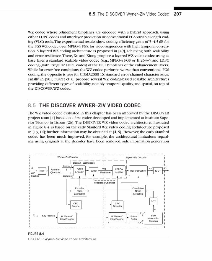
8.5 The DISCOVER Wyner–Ziv Video Codec 207
WZ codec where refinement bit-planes are encoded with a hybrid approach, usingeither LDPC codes and interlayer prediction or conventional FGS variable-length cod-ing (VLC) tools.The experimental results show coding efficiency gains of 3–4.5 dB forthe FGS WZ codec over MPEG-4 FGS, for video sequences with high temporal correla-tion. A layered WZ coding architecture is proposed in [49], achieving both scalabilityand error resilience. There, Xu and Xiong propose a layered WZ video codec using asbase layer, a standard scalable video codec (e.g., MPEG-4 FGS or H.263+), and LDPCcoding (with irregular LDPC codes) of the DCT bit-planes of the enhancement layers.While for error-free conditions, the WZ codec performs worse than conventional FGScoding, the opposite is true for CDMA2000 1X standard error channel characteristics.Finally, in [50], Ouaret et al. propose several WZ coding-based scalable architecturesproviding different types of scalability, notably temporal, quality, and spatial, on top ofthe DISCOVER WZ codec.
8.5 THE DISCOVER WYNER–ZIV VIDEO CODECThe WZ video codec evaluated in this chapter has been improved by the DISCOVERproject team [4] based on a first codec developed and implemented at Instituto Supe-rior Técnico in Lisbon [26]. The DISCOVER WZ video codec architecture, illustratedin Figure 8.4, is based on the early Stanford WZ video coding architecture proposedin [13, 14]; further information may be obtained at [4, 5]. However, the early Stanfordcodec has been much improved, for example, the architectural limitations regard-ing using originals at the decoder have been removed, side information generation
Wyner–Ziv DecoderWyner–Ziv Encoder
Slepian–Wolf codec
UniformQuantizer . .
.
Yi
X ¢ b
X ¢ f
LDPCAEncoder
LDPCADecoderBufferDCT
DCT
H.264/AVCIntra Encoder
FrameBuffer
H.264/AVCIntra Decoder
Xi 1m Key Frames
WZFrames
SideInformation
Creation
Xi DCT ¢i
IDCTReconstruction
CRCDecoder
CRCEncoder
CorrelationNoise
Modeling
EncoderRate
Estimation
X ¢i
Bitstream
Feedback Channel
Bitplane 1WZ
Bitplane Mb
FIGURE 8.4
DISCOVER Wyner–Ziv video codec architecture.
208 CHAPTER 8 Distributed Video Coding: Basics, Codecs, and Performance
and reconstruction have been improved, and an LDPCA code has been added forSlepian–Wolf coding and a CRC code for error detection. In practice, the tools formost of theWZ architecture modules are different (and globally much more efficient).
The DISCOVER codec is probably the most efficientWZ video codec now available.Its performance is reported in detail with the corresponding test conditions in [4];moreover, executable code may be downloaded, allowing all researchers to compareperformances for other sequences and conditions as well.
The DISCOVER WZ video codec works as follows:
At the encoder:1. Frame Classification First, a video sequence is divided into WZ frames; this
means the frames that will be coded using a WZ approach, and key framesthat will be coded as Intra frames (e.g., using the H.264/AVC Intra codec[1]). Typically key frames are periodically inserted with a certain GOP size.An adaptive GOP size selection process may also be used, meaning that thekey frames are inserted depending on the amount of temporal correlation inthe video sequence [27]. Most results available in the literature use a GOP sizeof 2, which means that odd and even frames are key frames and WZ frames,respectively.
2. Discrete Cosine Transform Over each Wyner–Ziv frame, an integer 4�4 block-based DCT is applied. The DCT coefficients of the entire WZframe are then grouped together, according to the position occupied byeach DCT coefficient within the 4�4 blocks, forming the DCT coefficientsbands.
3. Quantization After the transform coding operation, each DCT coefficientsband bk is uniformly quantized with 2Mk levels (where the number of levels2Mk depends on the DCT coefficients band bk). Over the resulting quantizedsymbol stream (associated with the DCT coefficients band bk),bit-plane extrac-tion is performed. For a given band, the quantized symbols bits of the samesignificance (e.g., the most significant bit) are grouped together, forming thecorresponding bit-plane array, which is then independently LDPC (or turbo)encoded [22].
4. LDPCA Encoding The LDPCA (or turbo) encoding procedure for the DCTcoefficients band bk starts with the most significant bit-plane array, which cor-responds to the most significant bits of the bk band quantized symbols. Theparity information generated by the LDPCA encoder for each bit-plane is thenstored in the buffer and sent in chunks/packets upon decoder request, throughthe feedback channel.
5. Encoder Rate Estimation In order to limit the number of requests to bemade by the decoder, and thus the decoding complexity and transmissiondelay (since each request corresponds to several LDPC decoder iterations),the encoder estimates for each bit-plane the initial number of bits to be sent
8.5 The DISCOVER Wyner–Ziv Video Codec 209
before any request is made [5]. This number should be an underestimation ofthe final number of bits needed if no RD performance losses associated withthis step are welcome (regarding the pure decoder rate control case). If therate is underestimated, the decoder will complement it by making one or morerequests.
At the decoder:6. Side Information Creation The decoder creates the side information for
each WZ coded frame with a motion-compensated frame interpolation frame-work, using the previous and next temporally closer reference frames togenerate an estimate of the WZ frame [26, 27]. The side information for eachWZ frame corresponds to an estimation of the original WZ frame. The betteris the quality of this estimation, the smaller are the number of “errors” theWZ LDPC (or turbo) decoder has to correct and the bit rate necessary forsuccessful decoding (i.e., with a small error probability).
7. DCT Estimation A block-based 4�4 DCT is then carried out over the sideinformation in order to obtain the DCT coefficients, which are an estimate ofthe WZ frame DCT coefficients.
8. Correlation Noise Modeling The residual statistics between correspondingWZ frame DCT coefficients and the side information DCT coefficients areassumed to be modeled by a Laplacian distribution. The Laplacian parameteris estimated on-line and at different granularity levels, notably at band andcoefficient levels [31, 32].
9. LDPCA Decoding Once the DCT-transformed side information and the resid-ual statistics for a given DCT coefficients band bk are known, the decodedquantized symbol stream associated with the DCT band bk can be obtainedthrough the LDPCA decoding procedure. The LDPCA (or turbo) decoderreceives from the encoder successive chunks of parity bits following therequests made through the feedback channel [22].
10. Request Stopping CriterionTo decide whether or not more bits are neededfor the successful decoding of a certain bit-plane, the decoder uses a simplerequest stopping criterion, that is, checks that all LDPC code parity-checkequations are fulfilled for the decoded (hard decision) codeword. If no morebits are needed to decode the bit-plane, the decoding of the next bit-plane orband can start; otherwise, the bit-plane LDPC decoding task has to proceedwith another request and receive another chunk of parity bits.
11. Further LDPCA Decoding After successfully LDPCA (or turbo) decoding themost significant bit-plane array of the bk band, the LDPCA (or turbo) decoderproceeds in an analogous way to the remaining Mk�1 bit-planes associatedwith that band. Once all the bit-plane arrays of the DCT coefficients band bk
are successfully LDPCA (or turbo) decoded, the LDPCA (or turbo) decoder

210 CHAPTER 8 Distributed Video Coding: Basics, Codecs, and Performance
starts decoding the bk�1 band. This procedure is repeated until all the DCTcoefficients bands for which WZ bits are transmitted are LDPCA (or turbo)decoded.
12. CRC Checking Because some residual errors are left even when all parity-check equations are fulfilled (step 10) and may have a rather negativesubjective impact on the decoded frame quality, a CRC checksum is trans-mitted to help the decoder detect and correct the remaining errors in eachbit-plane. Since this CRC is combined with the developed request stoppingcriterion, it does not have to be very strong in order to guarantee a vanishingerror probability (≈ 0) for each decoded bit-plane. As a consequence,a CRC-8checksum for each bit-plane was found to be strong enough for this purpose,which only adds minimal extra rate (8 bits).
13. Symbol Assembling After LDPCA (or turbo) decoding, the Mk bit-planesassociated with the DCT band bk, the bit-planes are grouped together to formthe decoded quantized symbol stream associated with the bk band. This pro-cedure is performed over all the DCT coefficients bands to which WZ bits aretransmitted. The DCT coefficients bands for which no WZ bits were trans-mitted are replaced by the corresponding DCT bands from the DCT sideinformation.
14. Reconstruction Once all quantized symbol streams are obtained,it is possibleto reconstruct the matrix of decoded DCT coefficients for each block.
15. IDCT After a block-based 4�4 IDCT is performed, the reconstructed pixeldomain WZ frame is obtained.
16. Frame Remixing To finally get the decoded video sequence, decoded keyframes and WZ frames are mixed conveniently.
It is important to stress that the DISCOVER WZ video codec does not include anyof the limitations that are often still present in WZ video coding papers, notablythose adopting the StanfordWZ architecture.This means, for example, that no originalframes are used at the decoder to create the side information,to estimate the bit-planeerror probability or to estimate the correlation noise model parameters for LDPCA(or turbo) decoding. The DISCOVER WZ video codec is a fully practical video codecfor which a realistic performance evaluation was made [4]. For a better understand-ing of the DISCOVER WZ video codec, the next sections will provide some detail forthe main coding tools. For more details, the readers should consult the papers listedin [4].
8.5.1 Transform and Quantization
In the DISCOVER architecture, illustrated in Figure 8.4, the first stage toward encod-ing a Wyner–Ziv frame is transform coding (corresponding to the DCT module). Thetransform employed in the DISCOVER WZ video codec relies on an integer 4�4

8.5 The DISCOVER Wyner–Ziv Video Codec 211
block-based DCT transform,1 as defined by the H.264/AVC standard [1]. The DCTtransform is applied to all 4�4 nonoverlapping blocks of the WZ frame, from left toright and top to bottom.
Afterward,quantization is applied to each DCT coefficient band bk to exploit irrel-evance and achieve the target quality.Two different quantization approaches are usedin the DISCOVER solution.
1. DC Coefficients The DC coefficients band is quantized using a uniformscalar quantizer without a symmetric quantization interval around the zeroamplitude. Typically, the DC coefficients band is characterized by high-amplitude positive values since each DC transform coefficient expresses theaverage energy of the corresponding 4�4 samples block.
2. AC Coefficients The remaining AC coefficients bands are quantized using auniform scalar quantizer with quantized bins evenly distributed around zero inorder to reduce the block artifacts effect.The zero bin size is twice the remainingbins size. Since most of the AC coefficients are concentrated around zero, bydoubling the zero bin size, the matching probability between correspondingquantized bins of the WZ and SI frames increases, bringing bit rate savings.Some distortion loss is, however, expected since the larger the quantizationbin, the worset the decoded frame quality is, but overall the RD performanceimproves.
Moreover, the DISCOVER codec considers a varying quantization step size for theAC coefficients. The decoder is informed by the encoder of the dynamic range foreach AC band of each WZ frame.This allows a quantization bin width (step size) to beadjusted to the dynamic range of each AC band. Since the dynamic range of a givenAC band may be lower than a fixed selected value, a smaller quantization bin width isused in the DISCOVER codec, for the same number of quantization levels.The smallerthe quantization step size, the lower the distortion is at the decoder. In summary, theAC coefficients can be more efficiently encoded varying the quantization step sizeaccording to the dynamic range of each AC coefficients band. In the DISCOVER WZcodec, the quantization step size,W, for the AC bands bk(k�2, . . . , 16) is obtainedfrom W �2|Vk|max/(2Mk �1) where |Vk|max stands for the highest absolute valuewithin bk. For 4�4 samples blocks and 8-bit accuracy video data,the DC band dynamicrange is 1024. This value is maintained fixed for all the video frames.
8.5.2 Slepian–Wolf Coding
The DISCOVER WZ video codec has adopted a class of LDPC codes for the Slepian–Wolf part of the WZ codec after using the popular turbo codes for a long time.The DISCOVER codec uses an LDPC Accumulate (LDPCA) codec, which consists of
1 To be more precise, a separable integer transform with similar properties as a 4�4 DCT is used.
212 CHAPTER 8 Distributed Video Coding: Basics, Codecs, and Performance
an LDPC syndrome code concatenated with an accumulator [22] to achieve a rate-compatible operation. For each bit-plane, syndrome bits are created using the LDPCsyndrome code and accumulated modulo 2 to produce the accumulated syndrome.Basically,the LDPC syndrome encoder calculates for the input bit-plane x the syndromes �Hx,where H corresponds to the parity-check matrix.The parity-check matrix H ofthe LDPC code represents the connections (i.e., edges) of a bipartite graph with twonode types:the variable nodes and the check nodes. It also has a sparse representation,that is,with a low density of 1’s,which guarantees a low encoder complexity.When anLDPC syndrome code is concatenated with an accumulator,the resulting concatenatedcode is rate adaptive and incremental, allowing the use of the request-decode strategyalready employed for the turbo codes. Thus, after the calculation of the accumulatedsyndromes, they are stored in a buffer and transmitted to the decoder in chunks,upondecoder request.
Making use of the side information created at the decoder (see Section 8.5.3), theLDPC syndrome decoder attempts to reconstruct the original data, with the help ofthe correlation noise model, using a soft-bit decoding belief propagation algorithmthat operates in bipartite graph (or equivalently matrix H) with high efficiency. In thiscase,the popular log-domain sum-product algorithm (SPA) is used with the adaptationsdescribed in [21] for LDPC syndrome codes with side information available at thedecoder. The SPA algorithm uses an iterative approach and consists of exchangingmessages along the edges, from variable nodes initialized with the correlation noisemodel soft-input information, to check nodes, which are affected by the receivedsyndromes. At each node type, different calculations are performed. Moreover, theyalways exchange extrinsic information, that is, outgoing messages at an edge do notconsider incoming information on the same edge.
If the number of syndrome bits is not enough,WZ decoding fails, the encoder isnotified by the feedback channel and more accumulated syndromes are sent from theencoder buffer. To enable this type of rate control, the LDPCA decoder tests the con-vergence by computing the syndrome check error—that is, by counting the numberof parity-check equations that are not satisfied, assuming a certain decoded bit-planeby the SPA. In fact, the syndrome check error is calculated after each LDPC decod-ing iteration. If the syndrome check error is different from zero and the maximumnumber of iterations was not reached, another LDPC decoding iteration will start: inthis case up to 100 iterations are allowed. After 100 iterations, if the syndrome checkerror remains different from zero, the decoded bit-plane is assumed to be erroneouslydecoded, and the LDPCA decoder requests more accumulated syndromes. If at anytime the syndrome check error is equal to zero, a CRC mechanism is used to detectif there are remaining errors in the decoded bit-plane. The CRC-8 checksum is com-puted by the encoder for every encoded bit-plane and transmitted to the decoder. If thedecoded bit-plane has the same CRC checksum that the encoder CRC checksum has,the decoding is declared to be successful and the decoding of another band/bit-planecan start. Note also that the inverse of the H matrix is used when all syndrome bits arereceived (compression ratio of 1:1),allowing recovery of the source,losslessly,since His full rank and the LDPC syndrome code is linear.This is a significant advantage when
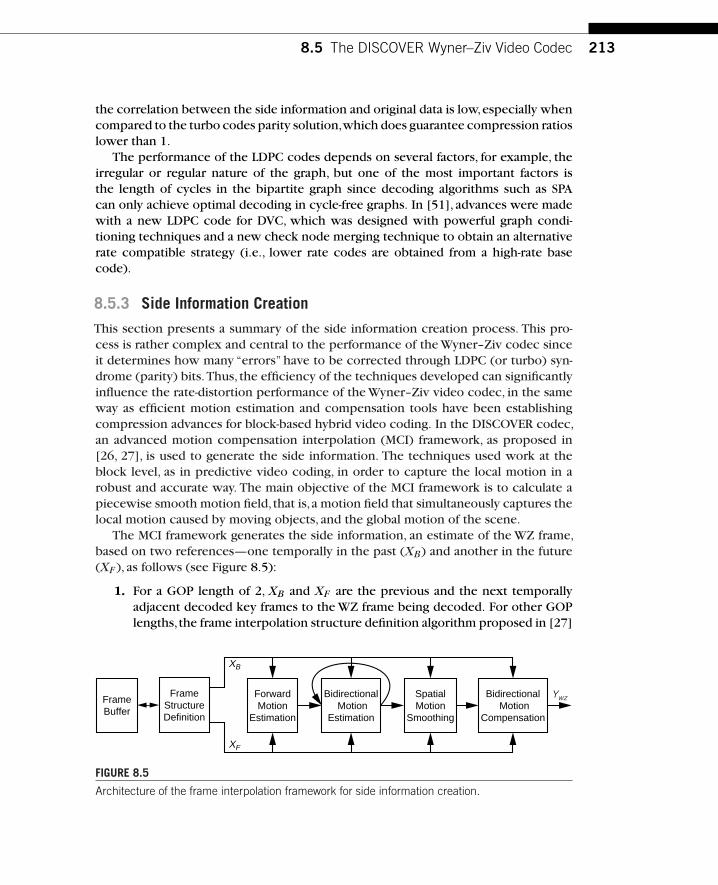
8.5 The DISCOVER Wyner–Ziv Video Codec 213
the correlation between the side information and original data is low,especially whencompared to the turbo codes parity solution,which does guarantee compression ratioslower than 1.
The performance of the LDPC codes depends on several factors, for example, theirregular or regular nature of the graph, but one of the most important factors isthe length of cycles in the bipartite graph since decoding algorithms such as SPAcan only achieve optimal decoding in cycle-free graphs. In [51], advances were madewith a new LDPC code for DVC, which was designed with powerful graph condi-tioning techniques and a new check node merging technique to obtain an alternativerate compatible strategy (i.e., lower rate codes are obtained from a high-rate basecode).
8.5.3 Side Information Creation
This section presents a summary of the side information creation process. This pro-cess is rather complex and central to the performance of the Wyner–Ziv codec sinceit determines how many “errors” have to be corrected through LDPC (or turbo) syn-drome (parity) bits.Thus, the efficiency of the techniques developed can significantlyinfluence the rate-distortion performance of the Wyner–Ziv video codec, in the sameway as efficient motion estimation and compensation tools have been establishingcompression advances for block-based hybrid video coding. In the DISCOVER codec,an advanced motion compensation interpolation (MCI) framework, as proposed in[26, 27], is used to generate the side information. The techniques used work at theblock level, as in predictive video coding, in order to capture the local motion in arobust and accurate way. The main objective of the MCI framework is to calculate apiecewise smooth motion field, that is,a motion field that simultaneously captures thelocal motion caused by moving objects, and the global motion of the scene.
The MCI framework generates the side information, an estimate of the WZ frame,based on two references—one temporally in the past (XB) and another in the future(XF ), as follows (see Figure 8.5):
1. For a GOP length of 2, XB and XF are the previous and the next temporallyadjacent decoded key frames to the WZ frame being decoded. For other GOPlengths,the frame interpolation structure definition algorithm proposed in [27]
FrameBuffer
FrameStructureDefinition
ForwardMotion
Estimation
BidirectionalMotion
Estimation
BidirectionalMotion
Compensation
SpatialMotion
Smoothing
Ywz
XB
XF
FIGURE 8.5
Architecture of the frame interpolation framework for side information creation.

214 CHAPTER 8 Distributed Video Coding: Basics, Codecs, and Performance
indicates the decoding order and the reference frames to be used by the frameinterpolation algorithm.
2. Both reference frames, XB and XF , are first low-pass filtered to improve thereliability of the motion vectors. Then, a block-matching algorithm is used toestimate the motion between the XB and XF frames. In this step, full-searchmotion estimation with modified matching criteria is performed [26]; the crite-ria include a regularized term that favors motion vectors that are closer to theorigin.
3. The bidirectional motion estimation module refines the motion vectors obtainedin the previous step with an additional constraint: the motion vector selectedfor each block has a linear trajectory between the next and previous referenceframes and crosses the interpolated frame at the center of the blocks. Thistechnique combines a hierarchical block-size technique with a new adaptivesearch range strategy in a very efficient way [27].The hierarchical coarse-to-fineapproach tracks fast motion and handles large GOP sizes in the first iteration(block size 16�16) and then achieves finer detail by using smaller block sizes(block size 8�8).
4. Next, a spatial motion smoothing algorithm based on weighted vector medianfilters [26] is used to make the final motion vector field smoother, except atobject boundaries and uncovered regions.
5. Once the final motion vector field is obtained, the interpolated frame can befilled by simply using bidirectional motion compensation as defined in standardvideo coding schemes.
This type of advanced frame interpolation solution has a major contribution tothe good RD performance of the DISCOVER WZ video codec since the quality of thegenerated side information has a crucial role in the overall codec RD performance.
8.5.4 Correlation Noise Modeling
To make good usage of the side information obtained through the frame interpolationframework, the decoder needs to have reliable knowledge of the model that charac-terizes the correlation noise between corresponding DCT bands of the WZ and sideinformation frames. The Laplacian distribution is widely used to model the residualstatistics between correspondent coefficients in XDCT
WZ and Y DCTWZ , for example, [14],
and, thus, it was also adopted by the DISCOVER WZ video codec. The Laplacian dis-tribution parameter � is estimated on-line at the decoder, for each DCT coefficient,using (2) below, based on the residual, R, between the reference frames XB and XF
used to create the side information after motion compensation [32]. Basically, afterapplying the 4�4 DCT transform over the R frame, each DCT coefficient is classifiedinto one of two classes: (1) inlier coefficients corresponding to those whose absolute

8.5 The DISCOVER Wyner–Ziv Video Codec 215
value (magnitude) is close to the corresponding R frame DCT band magnitude averagevalue �|b|; and (2) outlier coefficients corresponding to those whose magnitude is faraway from �|b|. To determine how close a certain coefficient is to the correspondingR frame DCT band magnitude average value, the distance between that coefficientmagnitude and �|b| with the DCT band magnitude variance �2|b| is compared since thevariance is a measure of how spread the coefficient values are regarding its averagevalue. The � parameter estimation in (2) leads to a finer adaptation of the correlationnoise model,both spatially (within a frame) and temporally (along the video sequence):
�b(u, v)�
⎧⎪⎨⎪⎩√
2�2
b,[D|b|(u, v)
]2� �2|b|√
2[D|b|(u,v)]2 ,
[D|b|(u, v)
]2� �2|b|
. (8.2)
In Equation (8.1), �b(u, v) is the � parameter estimate for the DCT coefficientlocated at (u, v) position, �2|b| is the estimate of the variance for the DCT band towhich the DCT coefficient belongs,and D|b|(u, v) represents the distance between the(u, v) coefficient magnitude and the DCT coefficients band b magnitude average value.The distance D|b|(u, v) measures how spread the coefficient’s values are regarding itscorresponding DCT band average value [32]. The first branch in (8.2) correspondsto a block/region well interpolated. Thus, the estimate of the � parameter for theR frame DCT band is a more reliable estimation in this case. The second branch in(8.2) corresponds to a block where the residual error is high,which means that the SIgeneration process failed for that block.Thus,the � parameter estimate for the R frameDCT band is not the best approach in this case,since it corresponds to an average valuefor all DCT coefficients within the band b. In this case, the solution adopted by theDISCOVER codec is to estimate �b(u, v) using [D|b|(u, v)]2 since this enables givingless confidence to the turbo decoder on the DCT coefficients that belong to blockswhere the frame interpolation algorithm essentially failed.
8.5.5 Reconstruction
The LDPC (or turbo) decoded bit-planes, together with the side information and theresidual statistics for each DCT coefficient band, are used by the reconstruction toobtain the decoded DCT coefficients matrix, XWZ
DCT as in [33]. Consider that theMk bit-planes associated with each DCT coefficients band, for which WZ bits werereceived, are successfully decoded. For each band, the bit-planes are grouped and adecoded quantization symbol (bin) q is obtained for each DCT coefficient, guidingthe decoder about where the original DCT coefficient value lies (an interval). Thedecoded quantization bin q corresponds to the true quantization bin q, obtained atthe encoder before bit-plane extraction, if all errors in the decoded bit-planes werecorrected (however, a very small error probability is allowed). The reconstructionfunction is optimal in the sense that it minimizes the mean-squared error (MSE)
216 CHAPTER 8 Distributed Video Coding: Basics, Codecs, and Performance
of the reconstructed value, for each DCT coefficient, of a given band and is givenby [33]
x�E[x|q, y
]�
∫ ul xfX | y(x| y)dx∫ ul fX | y(x| y)dx
(8.3)
where x is the reconstructed DCT coefficient, y is the corresponding DCT coeffi-cient of YWZ
DCT , E[.] is the expectation operator, and l and u represent the lowerand the upper bounds of q, respectively. In (8.3), the conditional probability densityfunction fX | y(.) models the residual statistics between corresponding coefficients inXWZ
DCT and YWZDCT . According to Section 8.3, fX | y(.) is typically assumed to be a
Laplacian distribution. After some analytical manipulations in (8.3), the reconstructedDCT coefficient can be obtained from (8.4) where corresponds to the quantizationbin size [33]. In (8.4), � is the Laplacian distribution parameter estimated on-line atthe decoder for each DCT coefficient (see Section 8.5.4).
x�
⎧⎪⎨⎪⎩l �b , y � l
y �(�� 1
�
)e����
(�� 1
�
)e���
2�e����e��� , y∈[l, u[ with b� 1� �
1�e� , � �y � l, ��u�yu�b , y�u
(8.4)
As can be seen in (8.4), the reconstruction function shifts the reconstructed DCTcoefficient value towards the center of the decoded quantization bin. The DCT coef-ficients bands to which no WZ bits are sent are replaced by the corresponding DCTbands of the side information.
8.6 THE DISCOVER CODEC PERFORMANCEThe target of this section is to perform a detailed evaluation of the DISCOVER WZvideo codec. With this purpose, precise test conditions are first defined. Afterward,the most relevant performance metrics to evaluate aWZ video codec will be assessed,notably: (i) RD performance; (ii) feedback channel rate performance; and (iii) codeccomplexity. For a more detailed performance evaluation, please see [4].
8.6.1 Performance Evaluation Conditions
Considering the main objective of this section, it is essential to meaningfully definethe performance evaluation conditions and the video codec control parameters inorder to set a clear and useful benchmarking. As usual in the DVC literature, only theluminance component is coded, and thus all metrics in this section refer only to theluminance. However, there are no reasons preventing use of the DISCOVERWZ codecfor the chrominance components with similar performance.
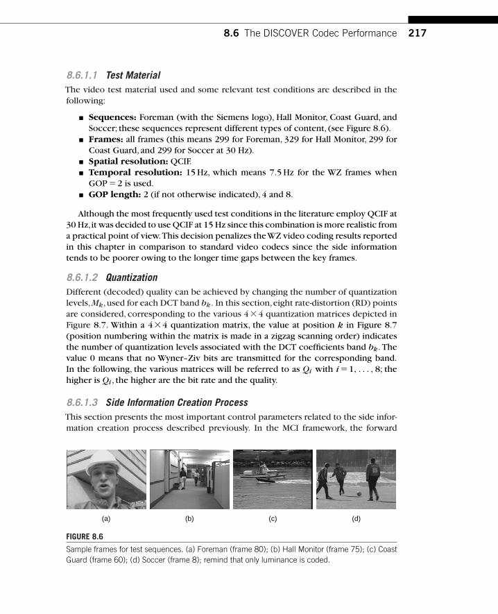
8.6 The DISCOVER Codec Performance 217
8.6.1.1 Test MaterialThe video test material used and some relevant test conditions are described in thefollowing:
■ Sequences: Foreman (with the Siemens logo), Hall Monitor, Coast Guard, andSoccer; these sequences represent different types of content, (see Figure 8.6).
■ Frames: all frames (this means 299 for Foreman, 329 for Hall Monitor, 299 forCoast Guard, and 299 for Soccer at 30 Hz).
■ Spatial resolution: QCIF.■ Temporal resolution: 15 Hz, which means 7.5 Hz for the WZ frames when
GOP �2 is used.■ GOP length: 2 (if not otherwise indicated), 4 and 8.
Although the most frequently used test conditions in the literature employ QCIF at30 Hz,it was decided to use QCIF at 15 Hz since this combination is more realistic froma practical point of view.This decision penalizes theWZ video coding results reportedin this chapter in comparison to standard video codecs since the side informationtends to be poorer owing to the longer time gaps between the key frames.
8.6.1.2 QuantizationDifferent (decoded) quality can be achieved by changing the number of quantizationlevels,Mk,used for each DCT band bk. In this section,eight rate-distortion (RD) pointsare considered, corresponding to the various 4�4 quantization matrices depicted inFigure 8.7. Within a 4�4 quantization matrix, the value at position k in Figure 8.7(position numbering within the matrix is made in a zigzag scanning order) indicatesthe number of quantization levels associated with the DCT coefficients band bk. Thevalue 0 means that no Wyner–Ziv bits are transmitted for the corresponding band.In the following, the various matrices will be referred to as Qi with i �1, . . . , 8; thehigher is Qi , the higher are the bit rate and the quality.
8.6.1.3 Side Information Creation ProcessThis section presents the most important control parameters related to the side infor-mation creation process described previously. In the MCI framework, the forward
(a) (b) (c) (d)
FIGURE 8.6
Sample frames for test sequences. (a) Foreman (frame 80); (b) Hall Monitor (frame 75); (c) CoastGuard (frame 60); (d) Soccer (frame 8); remind that only luminance is coded.

218 CHAPTER 8 Distributed Video Coding: Basics, Codecs, and Performance
16
8
0
0
8
0
0
0
0
0
0
0
0
0
0 0
32
16
8
4
16
8
4
4
4
4
0
4
0
0
8 4 64
16
8
8
16
8
8
4
8
4
4
4
4
0
8 8 64
32
16
8
32
16
8
4
8
4
4
4
4
0
16 8 128
64
32
16
64
32
16
8
16
8
4
8
4
0
32 16
32
8
0
0
8
0
0
0
0
0
0
0
0
0
0 0 32
8
4
0
8
4
0
0
0
0
0
0
0
0
4 0 32
16
8
4
16
8
4
0
4
0
0
0
0
0
8 4
(a) (b) (c) (d)
(e) (f) (g) (h)
FIGURE 8.7
Eight quantization matrices associated with different RD points.
motion estimation works with 16�16 block sizes, and �32 pixels are used for thesearch range. In the second iteration of the bidirectional motion estimation,the motionvectors are refined using 8�8 block sizes, and an adaptive search range is used torestrict the motion vector trajectory to be close to the neighboring motion vectorswhile still leaving room to increase its accuracy and precision. The motion search isperformed using the half-pixel precision, and the reference frames are first low-passfiltered with the mean filter using a 3�3 mask size.
8.6.1.4 Key Frames CodingThe key frames are always encoded with H.264/AVC Intra (Main profile) because thisis the best performing Intra video coding standard available.The key frames are codedwith constant quantization parameters (QP) as defined in Table 8.1. The key framesquantization parameters have been found using an iterative process that stops whenthe average quality (PSNR) of the WZ frames is similar to the quality of the Intraframes (H.264/AVC coded). The values in Table 8.1 have been obtained for GOP �2,QCIF@15 Hz. The selection of these QP values for the key frames was made with thetarget being to have almost constant (on average) decoded video quality for the fullset of frames (key frames and WZ frames).
Investing the same total bit rate in a different way betweenWZ and key frames maylead to a better overall RD performance. For example,by investing more bits in the keyframes, the overall RD performance may improve at the cost of a less stable (in time)

8.6 The DISCOVER Codec Performance 219
Table 8.1 Key Frames Quantization Parameters forthe Various RD Points for QCIF@15 Hz
Q1 Q2 Q3 Q4 Q5 Q6 Q7 Q8
Foreman 40 39 38 34 34 32 29 25
Hall Monitor 37 36 36 33 33 31 29 24
Coast Guard 38 37 37 34 33 31 30 26
Soccer 44 43 41 36 36 34 31 25
video quality. This is a choice to be made by the encoder knowing the consequencesin terms of subjective impact. For comparison purposes, the QP values in Table 8.1will be used all along this section under the assumption stated above.
8.6.2 RD Performance Evaluation
This section targets RD performance evaluation. This means the assessment of howthe rate for the key frames (H.264/AVC Intra bits) and the rate for the WZ frames(LDPC syndrome bits + CRC bits) translates into quality. All metrics regard both thekey frames andWZ frames bits since they correspond to the overall decoded quality. Inthis section, error-free channels are considered, but it is well acknowledged that DVCsolutions are especially interesting when error resilience is a critical requirement. Adetailed error resilience performance evaluation is available in [45], and a detailedperformance evaluation as a function of the GOP size is available in [52].
8.6.2.1 Measuring the Overall Rate-distortion Performance
Defining the MetricsAlthough many metrics are relevant to evaluate the compression efficiency perfor-mance, it is recognized that the most frequently used quality metric is the averagePSNR (with all the well known limitations it implies) over all the frames of a videosequence coded for a certain quantization matrix (as defined in Section 8.6.1.2).Whenthe (luminance) PSNR metric is represented as a function of the used bit rate—in thiscase, the overall bit rate for the luminance component—very important performancecharts are obtained since they allow to easily compare the overall RD performancewith other coding solutions, including standard coding solutions largely well knownand used.
In this section, the RD performance of the DISCOVER WZ codec is comparedwith the corresponding performance of three standard coding solutions that sharean important property in terms of encoder complexity: the complex and expensivemotion estimation task is not performed by any of them. Section 8.6.3 will present the

220 CHAPTER 8 Distributed Video Coding: Basics, Codecs, and Performance
codec complexity evaluation that complements the RD evaluation proposed in thissection.
The three state-of-the-art standard solutions used in this section for comparisonpurposes are:
■ H.263+ Intra H.263+ video coding without exploiting temporal redundancy;this “Intra comparison” is still the one that appears most in the DVC literaturebut H.263+ Intra is clearly no longer the best standard Intra coding available andthus “beating” H.263+ Intra is much easier than “beating” H.264/AVC Intra (ofcourse, their encoding complexity is also rather different).
■ H.264/AVC Intra H.264/AVC video coding in Main profile without exploitingthe temporal redundancy; this type of Intra coding is the most efficient Intra(video) coding standard solution, even more than JPEG2000 for many condi-tions. However, it is important to notice that H.264/AVC Intra ( JM9.5 referencesoftware) exploits quite efficiently the spatial correlation (at a higher encodingcomplexity cost when compared to H.263+ Intra) with several 4�4 and 16�16Intra spatial prediction modes, a feature that is (still) missing in the DISCOVERWZ codec.
■ H.264/AVC Inter No Motion Video coding with H.264/AVC in Main profile( JM9.5 reference software) exploiting temporal redundancy in a IB. . .IB. . . struc-ture (depending on GOP size) but without performing any motion estimation,which is the most computationally expensive encoding task. The so-called NoMotion coding mode typically achieves better performance than Intra codingbecause it can partly exploit the temporal redundancy by using a DPCM temporalscheme. Moreover, it requires far less complexity than full-motion compensatedInter coding because no motion search is performed. This type of comparison(excluding encoder motion estimation as in WZ coding) is not typically pro-vided in most DVC published papers because it is still difficult to “beat” the RDperformance of H.264/AVC Inter No Motion with DVC-based solutions.
Results and AnalysisFigures 8.8 and 8.9 show the RD performance,according to the test conditions,for thefour test video sequences selected;also an RD performance comparison for GOP sizes2, 4, and 8 is presented. For these results, the following conclusions can be drawn:
■ DISCOVER codec vs. H.263+ Intra Coding For the Coast Guard and Hall Mon-itor sequences, coding gains exist for all RD points and for all GOP sizes withaverage gains up to 9 dB (for the Hall Monitor sequence at GOP �4) when com-pared to H.263+ Intra. Therefore, it is possible to conclude that the DISCOVERcodec can exploit (at least partly) the temporal correlation in the video content.On the other hand,for the Foreman sequence,the gains are not as impressive forGOP �2 (3 dB) and decrease when the GOP size increases; for GOP �8,a minorcoding loss is observed. The major reason is that for content with high andmedium motion, when the key frames are separated by a long gap in time, theside information quality decreases (and thus the overall RD performance) since

8.6
TheD
ISCO
VERC
odecP
erformance
22
1
Coast Guard
26
28
30
32
34
36
38
50 100 150 200 250 300 350 400 450 500 550 600
Rate [kbps]
PS
NR
[d
B]
DISCOVER H.264/AVC (Intra)H.2631 (Intra) H.264/AVC (No Motion)
Hall Monitor
24
26
28
30
32
34
36
38
40
42
50 100 150 200 250 300 350 400 450
Rate [kbps]
PS
NR
[d
B]
DISCOVER H.264/AVC (Intra)H.2631 (Intra) H.264/AVC (No Motion)
Soccer
26
28
30
32
34
36
38
40
0 50 100 150 200 250 300 350 400 450 500
Rate [kbps]
PS
NR
[d
B]
DISCOVER H.264/AVC (Intra)H.2631 (Intra) H.264/AVC (No Motion)
Foreman
26
28
30
32
34
36
38
40
50 100 150 200 250 300 350 400 450 500 550 600
Rate [kbps]P
SN
R [
dB
]
DISCOVER H.264/AVC (Intra)H.2631 (Intra) H.264/AVC (No Motion)
FIGURE 8.8
RD performance for GOP � 2: Coast Guard, Hall Monitor, Soccer, and Foreman (QCIF at 15 Hz).
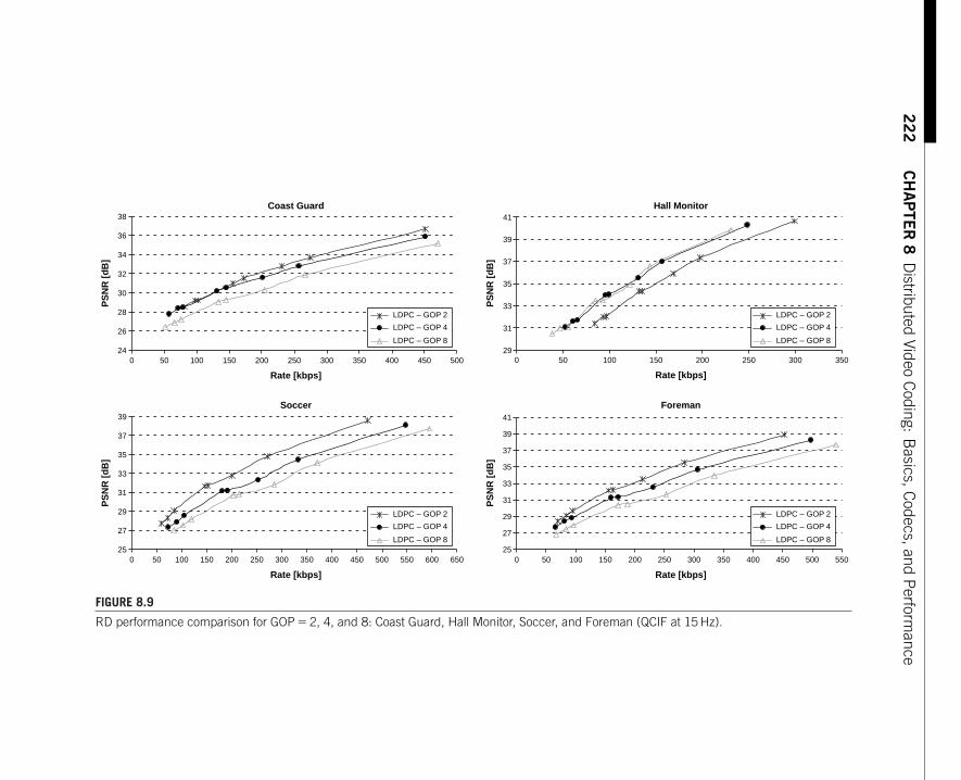
22
2C
HA
PTE
R8
Distributed
VideoC
oding:B
asics,Codecs,and
Perform
ance
Coast Guard
24
26
28
30
32
34
36
38
0 50 100 150 200 250 300 350 400 450 500
Rate [kbps]
PS
NR
[d
B]
LDPC – GOP 2
LDPC – GOP 4
LDPC – GOP 8
Hall Monitor
29
31
33
35
37
39
41
0 50 100 150 200 250 300 350
Rate [kbps]
PS
NR
[d
B]
Soccer
25
27
29
31
33
35
37
39
0 50 100 150 200 250 300 350 400 450 500 550 600 650
Rate [kbps]
PS
NR
[d
B]
Foreman
25
27
29
31
33
35
37
39
41
0 50 100 150 200 250 300 350 400 450 500 550
Rate [kbps]
PS
NR
[d
B]
LDPC – GOP 2
LDPC – GOP 4
LDPC – GOP 8
LDPC – GOP 2
LDPC – GOP 4
LDPC – GOP 8
LDPC – GOP 2
LDPC – GOP 4
LDPC – GOP 8
FIGURE 8.9
RD performance comparison for GOP � 2, 4, and 8: Coast Guard, Hall Monitor, Soccer, and Foreman (QCIF at 15 Hz).

8.6 The DISCOVER Codec Performance 223
it is more difficult to predict the frames in between. The worst performanceis achieved for the Soccer sequence, for all GOP sizes, since it is always belowH.263+ Intra. The major reason for this loss is the complex and erratic motionthat normally leads to a significant amount of errors in the side information andcauses a poorer RD performance, especially when the GOP size is quite large(8 frames at 15 fps correspond to more than half a second in a Soccer game).It is important to notice that better RD performance results would be obtainedfor 30 Hz, which is the most reported condition in the literature.
■ DISCOVER codec vs. H.264/AVC Intra Coding In this case, the DISCOVERcodec is compared to the best performing (video) Intra encoder available, theH.264/AVC Intra codec. The Hall Monitor sequence has the best performance,with consistent gains for all GOP sizes (up to 4 dB). The Coast Guard sequenceat GOP �2 has gains up to 1 dB, and some RD points for the Foreman sequence(GOP �2) show minor gains.The rest of the sequence@GOP size combinationshave a lower performance when compared to H.264/AVC Intra; in these cases,the difficulty is to obtain good side information for high motion sequences withlarge GOP sizes. However, the results are quite encouraging since for a signifi-cant amount of (sequence@GOP size) scenarios,the DISCOVER RD performancebeats H.264/AVC Intra;notably, for GOP �2, the DISCOVER codec only loses forthe Soccer sequence, which is a rather difficult sequence to be coded at 15 Hz.It is also important to note that the H.264/AVC Intra codec includes several spa-tial prediction modes, RD optimization, and advanced entropy coding tools asCABAC in order to achieve a higher RD performance (at some encoding com-plexity cost). So, the conclusion to be confirmed in Section 8.6.3 is that theDISCOVER codec can, for most cases at GOP �2, achieve better performancewith lower encoding complexity.
■ DISCOVER codec vs. H.264/AVC Inter No Motion Coding In this case, theDISCOVER codec is compared to a low complexity Inter codec (compared to fullH.264/AVC Inter) that is still able to exploit some temporal correlation.An inter-esting observation is that the H.264/AVC No Motion curve is very close to theH.264/AVC Intra curve for the Soccer and Coast Guard sequences (for all GOPsizes) and for the Foreman sequence at GOP �8. Since for these cases the tempo-ral correlation is quite low, the H.264/AVC No Motion solution selects the Intramode for the majority of the blocks (mode decision Intra/Inter is still allowed).The DISCOVER codec is quite competitive for the Coast Guard sequence wheresome gains (up to 1 dB) in comparison to H.264/AVC No Motion are observed.In such cases, the DISCOVER side information creation framework exploits veryefficiently the temporal correlation. However, for the Hall Monitor sequence,an RD loss is observed, especially for higher bit rates, where the H.264/AVCSKIP macroblock mode (no information other than the mode is coded) bringsadditional benefits for this low-motion sequence.
■ DISCOVER codec RD performance for different GOP Sizes For allsequences but Hall Monitor, GOP �2 wins, showing the difficulty in gettinggood side information for longer GOP sizes due to the decreased performance

224 CHAPTER 8 Distributed Video Coding: Basics, Codecs, and Performance
of the frame interpolation process. For Hall Monitor, which is a rather stablesequence, GOP �4 and GOP �8 are already more efficient than GOP �2 sincemotion estimation and frame interpolation are more reliable.
8.6.2.2 Comparing the RD Performance of LDPC and Turbo CodesDuring most of the DISCOVER project,the Slepian–Wolf codec part of the video codecwas based on turbo codes. Later, turbo codes were substituted by LDPC codes [22],essentially owing to their better RD performance and low complexity,especially at thedecoder side.
The turbo encoder enclosed a parallel concatenation of two identical constituentrecursive systematic convolutional (RSC) encoders of rate ½, and a pseudo-randomL-bit interleaver is employed to decorrelate the L-bit input sequence between thetwo RSC encoders. The pseudo-random interleaver length L corresponds to the DCTcoefficients band size, that is, the ratio between the frame size and the number ofdifferent DCT coefficients bands. Each RSC encoder outputs a parity stream and asystematic stream. For the turbo encoder, each rate ½ RSC encoder is represented by
the generator matrix[1 1�D�D3�D4
1�D3�D4
]and the trellis of the second RSC encoder is not
terminated. The puncturing period P is 48, which allows a fine-grained control of thebit rate. After turbo encoding a bit-plane of a given DCT coefficients band (startingwith the most significant bit-plane), the systematic part (a copy of the turbo encoderinput) is discarded, and the parity bits are stored in the buffer. Upon decoder request,the parity bits produced by the turbo encoder are transmitted according to a pseudo-random puncturing pattern. In each request, the WZ encoder sends one parity bit ineach P parity bit from each RSC encoder parity stream; each parity bit is sent onlyonce. The location of the parity bits to be sent in each request is pseudo-randomlygenerated (it is known at both the encoder and decoder).
The Slepian–Wolf decoder encloses an iterative turbo decoder constituted by twosoft-input soft-output (SISO) decoders. Each SISO decoder is implemented using theLogarithmic Maximum A Posteriori (Log-MAP) algorithm. Since an iterative turbodecoding is used, the extrinsic information computed by one SISO decoder becomesthe a priori information of the other SISO decoder.Through this information exchangeprocedure between the two SISO decoders, the a posteriori estimates of the data bitsare updated until the maximum number of iterations allowed for iterative decoding isreached.A confidence measure based on the a posteriori probabilities ratio (check [38]for more details) is used as an error-detection criterion to determine the current bit-plane error probability Pe of a given DCT band. If Pe is higher than 10�3, the decoderrequests for more parity bits from the encoder via the feedback channel; otherwise,the bit-plane turbo decoding task is considered successful.
Defining the MetricsThis section compares the RD performances of the turbo codes-based and LDPCcodes-based DISCOVER WZ codecs for equal conditions in terms of all othermodules.

8.6 The DISCOVER Codec Performance 225
Results and AnalysisFigure 8.10 shows the RD performance comparison between the DISCOVERWZ videocodecs using turbo codes and LDPC codes. Observing the RD performance curvesshown in Figure 8.10,it can be noticed that the LDPC codes always have better perfor-mance than turbo codes for all GOP sizes and all sequences.The following conclusionscan be drawn:
■ For lower bit rates,the performance of the turbo and LDPC codes is quite similarbecause when the correlation between the side information and the WZ framesis high, the turbo codes achieve a good performance and similar results to theLDPC codes.
■ For medium and high bit rates,the LDPC codes have a better performance whencompared to the turbo codes,with coding gains up to 35 kbps for GOP �8.TheLDPC codes show better performance for the bands/bit-planes, which have alow correlation between the side information and the WZ frame (i.e., for sideinformation with low quality).
■ When the GOP size increases,the performance gap between the turbo codes andthe LDPC codes increases,with a clear advantage for the LDPC codes (for GOP �2, 4, 8 coding gains up to 10, 27, 35 kbps occur, respectively). One major reasonfor this effect is that the LDPCA codes (as other types of LDPC codes) always havea maximum rate of 1,that is,the maximum number of syndrome bits sent cannotexceed the number of bits that represent the original data.This property comesfrom the code linear properties, which allow recovering the original sourceinformation when the rate is equal to 1 by solving the parity-check matrix equa-tions. This property does not exist for the iterative turbo codes (rate expansionis possible),and it is responsible for the turbo codes loss of efficiency,especiallyat larger GOP sizes,where the correlation between WZ and SI is lower and thuscompression rates higher than 1 are necessary to guarantee successful decoding.
8.6.2.3 Measuring the Bit-plane Compression FactorDefining the MetricsThe LDPCA syndrome encoder consists of an irregular LDPC encoder concatenatedwith an accumulator. The encoder buffers the accumulated syndrome and transmitsit incrementally to the decoder, following the decoder requests. The total number ofparity bits per bit-plane created by the LDPCA encoder is equal to the number of theinput bit-plane bits. This way the compression factor can only be higher than 1 (andnever lower than 1 as can happen for turbo codes); it allows measuring the capabilityof the DISCOVERWZ codec to compress the source data (bit-planes).The total averagecompression factor at frame,CFQ, and bit-plane,CFQij , levels for a certain quality level,Q, is given by (8.5) and (8.6):
CFQ �
BQ∑i�1
Mi∑j�1
N∑l�1
Cijl
wijl
N(8.5)
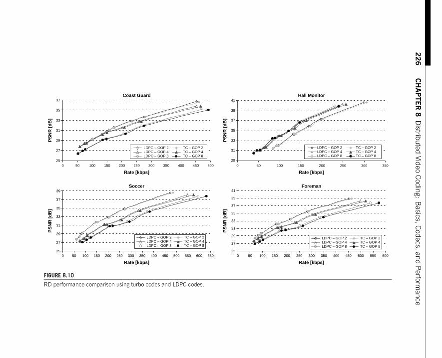
22
6C
HA
PTE
R8
Distributed
VideoC
oding:B
asics,Codecs,and
Perform
ance
Coast Guard
25
27
29
31
33
35
37
0 50 100 150 200 250 300 350 400 450 500
Rate [kbps]
PS
NR
[d
B]
LDPC – GOP 2 TC – GOP 2LDPC – GOP 4 TC – GOP 4LDPC – GOP 8 TC – GOP 8
Hall Monitor
29
31
33
35
37
39
41
0 50 100 150 200 250 300 350
Rate [kbps]
PS
NR
[d
B]
LDPC – GOP 2 TC – GOP 2LDPC – GOP 4 TC – GOP 4LDPC – GOP 8 TC – GOP 8
Soccer
25
27
29
31
33
35
37
39
0 50 100 150 200 250 300 350 400 450 500 550 600 650
Rate [kbps]
PS
NR
[d
B]
LDPC – GOP 2 TC – GOP 2LDPC – GOP 4 TC – GOP 4LDPC – GOP 8 TC – GOP 8
Foreman
25
27
29
31
33
35
37
39
41
0 50 100 150 200 250 300 350 400 450 500 550 600
Rate [kbps]
PS
NR
[d
B]
LDPC – GOP 2 TC – GOP 2LDPC – GOP 4 TC – GOP 4LDPC – GOP 8 TC – GOP 8
FIGURE 8.10
RD performance comparison using turbo codes and LDPC codes.

8.6 The DISCOVER Codec Performance 227
CFQij �
N∑l�1
Cijl
wijl
N (8.6)
where Mi is the number of bit-planes of each band i, N the total number of WZframes, Cijl the number of bits in each original coefficient bit-plane j of each band iat frame l, and wijl is the amount of parity bits sent for each bit-plane j of band i atframe l, BQ is the number of bands considering the quality level,Q. CFQij given by (8.6)represents the average compression factor at bit-plane j of band i for a certain qualitylevel Q.
Performing a study of the bit-plane compression factors for the various DCT coef-ficients bands is extremely useful because it allows detecting where inefficienciesare located to develop more advanced solutions. For example, it may allow locatingbands for which WZ coding is not efficient due to the lack of temporal correlation;this approach is followed by the PRISM codec [16].
Results and AnalysisFigure 8.11 shows the average bit-plane compression factor per band for Qi �4(medium bit rates) and 8 (high bit rates) for GOP �2 and for the four test videosequences. The following conclusions can be inferred:
■ In a general way, the least significant bit-planes (LSBs) have lower compressionfactors when compared to the most significant bit-planes (MSB and MSB-1).Thisbehavior is observed because the correlation between the side information andthe original bit-planes decreases when the bit-plane number index increases,especially for bands for which syndrome bits are sent for a high number ofbit-planes (e.g., DC and AC1-2). This suggests that more advanced quantizationand/or correlation noise models can further improve the performance in suchcases. Note that the compression factor is always greater than 1 and that bit rateexpansion does not occur for LDPC codes.
■ In a general way, for the AC bands, the highest compression factor is achievedfor the MSB-1. In this case, the decoder makes use of the a priori informationabout the decoding of the MSB (obtained through the correlation model). Sincethe MSB-1 and MSB are quite correlated,it is possible to achieve higher compres-sion factors. This correlation is lower for other bit-planes, and, therefore, lowercompression ratios are achieved.
■ The last AC bands usually have high compression ratios for both bit-planesbecause they only have four wide bins (2 bit-planes); therefore, the correlationbetween the side information and the WZ frame is high, and large compres-sion ratios can be achieved. When more bit-planes are considered in each band,the number of bins increases (and thus they are smaller) and more errorsoccur; that is, the mismatch between the side information bin and the WZframe bin increases (a low correlation is observed),decreasing the compressionfactor.

228 CHAPTER 8 Distributed Video Coding: Basics, Codecs, and Performance
DC
AC
9
AC
10
AC
11
AC
12
AC
13
AC
14
AC
8
AC
7
AC
5
AC
6
AC
4
AC
3
AC
2
AC
1
Co
mp
ress
ion
Fac
tor
212132132132143214321432143215432
Bitplane Number
Compression Factor (Qi5 8)
15432154321654321654321765432105
10152025303540 Coastguard Foreman
2121212132132132143214321543210
5
10
15
20
25
30
35
40
AC
9
AC
8
AC
7
AC
5
AC
6
AC
4
AC
3
AC
2
AC
9
AC
8
AC
7
AC
5
AC
6
AC
4
AC
3
AC
2
DC
Bitplane Number
Co
mp
ress
ion
Fac
tor
Compression Factor (Qi5 4)
Coastguard Foreman
AC
1
DC
AC
1
2121212132132132143214321543210
5
10
15
20
25
30
35
40
Bitplane Number
Co
mp
ress
ion
Fac
tor
Compression Factor (Qi5 4)
Hall Monitor Soccer
DC
AC
9
AC
10 AC
11
AC
12 AC
13
AC
14
AC
8
AC
7
AC
5
AC
6
AC
4
AC
3
AC
2
AC
1
Co
mp
ress
ion
Fac
tor
Hall Monitor Soccer
Bitplane Number
Compression Factor (Qi5 8)
05
10152025303540
1 2 3 4 5 6 7 1 2 3 4 5 6 1 2 3 4 5 6 1 2 3 4 5 1 2 3 4 5 1 2 3 4 5 1 2 3 4 1 2 3 4 1 2 3 4 1 2 3 4 1 2 3 1 2 3 1 2 3 1 2 1 2
FIGURE 8.11
Bit-plane compression factor for Qi � 4 and 8 (GOP � 2).

8.6 The DISCOVER Codec Performance 229
8.6.2.4 Measuring the Feedback Channel RateIn the DISCOVER WZ video coding architecture, the feedback channel has the roleto adapt the bit rate to the changing statistics between the side information (an esti-mation of the frame to be encoded) and the WZ frame to be encoded, that is, to thequality (or accuracy) of the frame interpolation process. Therefore, contrary to con-ventional codecs, it is the decoder’s responsibility to perform rate control and, in thisway, to guarantee that only a minimum number of parity bits are sent to correct themismatches/errors present in each side information bit-plane. The DISCOVER WZcodec does not use a pure decoder rate control but rather a hybrid rate control-approach,which means that fewer requests are made, lowering the feedback channelrate. Still, it is important to be aware of the feedback channel usage and impact inorder to design more efficient and lower complexity WZ video codecs.
Defining the MetricsIn order to measure the feedback channel rate for each DCT band and bit-plane, it isassumed that only one bit is required by the decoder to inform the encoder if moreparity bits are needed to successfully decode the current bit-plane. If more paritybits are needed, the decoder sends the bit “1” via the feedback channel; otherwise,the bit “0” is transmitted, and the encoder, receiving such bit, sends parity bits for thenext bit-plane to be decoded. This is clearly a simplistic solution since more bits areneeded,depending on the transmission protocol used;however, this simple approachis enough to have an idea on the feedback channel rate.
Since only one bit is transmitted via the feedback channel for each decoder request,the total feedback channel rate at frame RQ,and bit-plane RQij levels for a certain qualitylevel Q, can be obtained from (8.7) and (8.8), respectively.
RQ �
BQ∑i�1
Mi∑j�1
N∑l�1
nijl
N� f (8.7)
RQij �
N∑l�1
nijl
N� f (8.8)
In (8.7) and (8.8), f is the WZ frame rate and nijl is the number of bits sent via thefeedback channel for jth bit-plane of WZ frame l, DCT band i; N is the total numberof WZ frames,Mi is the number of bit-planes for DCT band i, and BQ is the number ofbands considering a certain quality level,Q. RQij is a partial result of (8.7),representingthe average feedback channel rate per frame for bit-plane j of DCT band i for a certainquality level Q.
Results and AnalysisFigure 8.12 shows the average feedback channel rate for Qi �4 and 8, for the fourselected video sequences, and for GOP �2. As can be observed, the number of bitssent through the feedback channel,for each band,increases with the bit-plane number

230 CHAPTER 8 Distributed Video Coding: Basics, Codecs, and Performance
21321 321 21 21 213214321432154320
1
20
40
60
80
100
120
140
160
AC
9
AC
8
AC
7
AC
5
AC
6
AC
4
AC
3
AC
2
DC
Rat
e [b
ps]
Bitplane Number
Feedback Channel Rate (Qi� 4)
Coastguard Foreman
AC
1
21321 321 21 21 213214321432154320
1
20
40
60
80
100
120
140
160
AC
9
AC
8
AC
7
AC
5
AC
6
AC
4
AC
3
AC
2
DC
Rat
e [b
ps]
Bitplane Number
Feedback Channel Rate (Qi� 4)
Hall Monitor SoccerA
C1
Hall Monitor Soccer
020406080
100120140160180
Rat
e [b
ps]
Feedback Channel Rate (Qi� 8)
Bitplane Number
Coastguard Foreman
321 654 217 543 6 21 543 6 21 543 321 154 432 215 143 432 321 214 143 132 132 13 2 1 22
321 654 217 543 6 21 543 6 21 543 321 154 432 215 143 432 321 214 143 132 132 13 2 1 22
0
20
40
60
80
100
120
140
160
Rat
e [b
ps]
Feedback Channel Rate (Qi� 8)
AC
9
AC
10
AC
11
AC
12
AC
13
AC
14
AC
8
AC
7
AC
5
AC
6
AC
4
AC
3
AC
2
DC
DC
AC
1
AC
9
AC
10
AC
11
AC
12
AC
13
AC
14
AC
8
AC
7
AC
5
AC
6
AC
4
AC
3
AC
2
AC
1
Bitplane Number
FIGURE 8.12
Feedback channel rate for Qi � 4 and 8 (GOP � 2).
to be decoded; the lower correlation between the side information and the WZ framefor LSB bit-planes is the main reason for that behavior.
Table 8.2 to Table 8.5 show the total feedback rate for the selected test sequencesfor each Qi for GOP �2, 4, and 8, respectively. It can easily be seen that the feedback

8.6 The DISCOVER Codec Performance 231
Table 8.2 Feedback Channel Rate (bps)for the Coast Guard Sequence
Qi GOP 2 GOP 4 GOP 8
1 132.59 327.36 551.85
2 179.94 437.61 697.66
3 216.34 525.05 853.44
4 377.68 996.63 1634.79
5 403.73 1075.75 1757.23
6 593.47 1565.25 2510.35
7 829.51 2150.83 3323.16
8 1514.88 3917.22 5835.58
Table 8.3 Feedback Channel Rate(bps) for the Hall Monitor Sequence
Qi GOP 2 GOP 4 GOP 8
1 109.60 222.51 321.82
2 146.09 294.29 417.55
3 173.04 362.08 574.15
4 263.69 606.95 978.49
5 289.79 665.22 1104.34
6 410.73 942.56 1485.84
7 512.53 1181.35 1761.99
8 821.26 1937.46 2804.30
Table 8.4 Feedback Channel Rate (bps)for the Soccer Sequence
Qi GOP 2 GOP 4 GOP 8
1 365.68 875.29 1250.50
2 430.33 1031.28 1455.37
3 498.08 1207.75 1723.70
4 857.81 2094.51 2974.20
5 919.06 2238.27 3175.56
6 1211.20 2925.92 4137.77
7 1542.28 3720.81 5242.56
8 2372.39 5663.22 7951.66
Table 8.5 Feedback Channel Rate(bps) for the Foreman Sequence
Qi GOP 2 GOP 4 GOP 8
1 222.49 580.70 889.67
2 284.64 722.59 1087.97
3 333.48 850.91 1282.86
4 590.37 1555.05 2367.78
5 663.12 1730.02 2629.46
6 916.41 2366.74 3553.20
7 1181.90 3065.26 4609.26
8 1937.21 4935.68 7266.50
channel rate is rather negligible; the maximum feedback channel rate correspondsto less than 8 kbps for Qi �8, for GOP �8, for the sequence Soccer (as expectedsince Soccer has the worse side information due to the high motion). Although itis not shown, the hybrid encoder/decoder rate control plays a central role, low-ering the feedback channel rate when compared to a pure decoder rate controlsolution.

232 CHAPTER 8 Distributed Video Coding: Basics, Codecs, and Performance
8.6.3 Complexity Performance Evaluation
Because evaluating the RD performance addresses only one side of the problem, thissection intends to perform an evaluation of the complexity performance for theDISCOVER WZ video codec. Although it is commonly claimed that DVC “encodingcomplexity is low” and “decoding complexity is high,” few complexity evaluationresults are available in the literature.
While it is possible to measure the encoding and decoding complexities in manyways, some of them rather sophisticated, it is also possible to get a rather good esti-mation of relative complexities using rather simple complexity metrics. Here, theencoding and decoding complexities will be measured by means of the encoding anddecoding times for the full sequence, in seconds, under controlled conditions. It iswell known that the encoding (and decoding) times are highly dependent on the usedhardware and software platforms. For the present results, the hardware used was anx86 machine with a dual core Pentium D processor at 3.4 GHz with 2048 MB of RAM.Regarding the software conditions,the results were obtained with aWindows XP oper-ating system, with the C++ code written using version 8.0 of the Visual Studio C++compiler,with optimizations parameters on, such as the release mode and speed opti-mizations. Besides the operating system, nothing was running in the machine whengathering the performance results to avoid influencing them. Under these conditions,the results have a relative and comparative value, in this case allowing comparing theDISCOVER WZ video codec with alternative solutions, for example, H.264/AVC JM9.5reference software, running in the same hardware and software conditions. While thedegree of optimization of the software has an impact on the running time, this is adimension that was impossible to fully control in this case and thus will have to bekept in mind when dealing with the provided performance results.
8.6.3.1 Measuring the Encoding ComplexityThis section targets the complexity evaluation of the encoding process. The encod-ing complexity includes two major components: the WZ frames encoding and thekey frames encoding parts. The larger the GOP size, the smaller the number of keyframes coded and, thus, the lower will be the share of the key frames in the overallcomplexity.
Defining the MetricsAlthough it is possible to measure the encoding complexity in many ways, some ofthem rather sophisticated, it is also possible to get a rather good “feeling” of relativecomplexities using rather simple complexity metrics. In this section, the encodingcomplexity will be measured by the encoding time for the full sequence, in seconds,under the conditions stated above.
Results and AnalysisFigure 8.13 and Table 8.6 to Table 8.9 show the encoding complexity results for var-ious GOP sizes measured in terms of encoding time, distinguishing between key
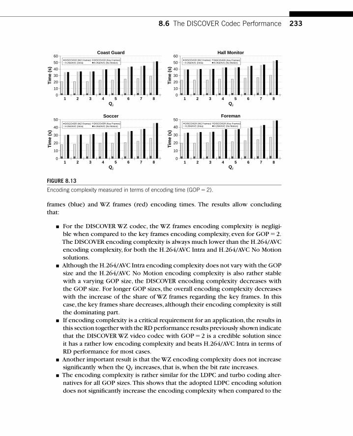
8.6 The DISCOVER Codec Performance 233
DISCOVER (WZ Frames)H.264/AVC (Intra)
DISCOVER (Key Frames)H.264/AVC (No Motion)
Coast Guard
Qi
60
50
40
30
Tim
e (s
)
20
10
021 3 4 5 6 7 8
DISCOVER (WZ Frames)H.264/AVC (Intra)
DISCOVER (Key Frames)H.264/AVC (No Motion)
Soccer
Qi
50
40
30
Tim
e (s
)
20
10
021 3 4 5 6 7 8
DISCOVER (WZ Frames)H.264/AVC (Intra)
DISCOVER (Key Frames)H.264/AVC (No Motion)
Foreman
Qi
50
40
30
Tim
e (s
)
20
10
021 3 4 5 6 7 8
DISCOVER (WZ Frames)H.264/AVC (Intra)
DISCOVER (Key Frames)H.264/AVC (No Motion)
Hall Monitor
Qi
60
50
40
30
Tim
e (s
)
20
10
021 3 4 5 6 7 8
FIGURE 8.13
Encoding complexity measured in terms of encoding time (GOP � 2).
frames (blue) and WZ frames (red) encoding times. The results allow concludingthat:
■ For the DISCOVER WZ codec, the WZ frames encoding complexity is negligi-ble when compared to the key frames encoding complexity, even for GOP �2.The DISCOVER encoding complexity is always much lower than the H.264/AVCencoding complexity, for both the H.264/AVC Intra and H.264/AVC No Motionsolutions.
■ Although the H.264/AVC Intra encoding complexity does not vary with the GOPsize and the H.264/AVC No Motion encoding complexity is also rather stablewith a varying GOP size, the DISCOVER encoding complexity decreases withthe GOP size. For longer GOP sizes, the overall encoding complexity decreaseswith the increase of the share of WZ frames regarding the key frames. In thiscase, the key frames share decreases, although their encoding complexity is stillthe dominating part.
■ If encoding complexity is a critical requirement for an application, the results inthis section together with the RD performance results previously shown indicatethat the DISCOVER WZ video codec with GOP �2 is a credible solution sinceit has a rather low encoding complexity and beats H.264/AVC Intra in terms ofRD performance for most cases.
■ Another important result is that the WZ encoding complexity does not increasesignificantly when the Qi increases, that is, when the bit rate increases.
■ The encoding complexity is rather similar for the LDPC and turbo coding alter-natives for all GOP sizes. This shows that the adopted LDPC encoding solutiondoes not significantly increase the encoding complexity when compared to the

23
4C
HA
PTE
R8
Distributed
VideoC
oding:B
asics,Codecs,and
Perform
ance
Table 8.6 Encoding Time (s) Comparison for the Coast Guard Sequence
H.264/AVC DISCOVER Ratios
Intra No Motion Using LDPC Codes Using Turbo Codes H.264/AVC Intra vs.DISCOVER LDPC
QP GOP 2 GOP 4 GOP 8 GOP 2 GOP 4 GOP 8 GOP 2 GOP 4 GOP 8 GOP 2 GOP 4 GOP 8
38 35.04 35.36 35.63 34.89 20.58 12.22 8.28 20.31 11.84 7.88 1.70 2.87 4.23
37 36.10 36.31 36.59 35.86 21.07 12.47 8.53 20.81 12.06 8.09 1.71 2.90 4.23
37 36.12 36.33 36.59 35.86 21.11 12.56 8.63 20.81 12.16 8.17 1.71 2.88 4.18
34 39.22 39.53 39.89 39.02 22.74 13.52 9.06 22.41 13.04 8.57 1.72 2.90 4.33
33 40.43 40.88 41.28 40.52 23.25 13.77 9.31 22.92 13.30 8.79 1.74 2.94 4.34
31 43.35 43.64 43.89 42.98 24.79 14.70 9.83 24.46 14.21 9.31 1.75 2.95 4.41
30 44.47 45.13 45.39 44.56 25.49 15.14 10.22 25.10 14.61 9.63 1.74 2.94 4.35
26 51.29 51.88 52.31 51.13 29.09 17.31 11.52 28.72 16.67 10.91 1.76 2.96 4.45

8.6
TheD
ISCO
VERC
odecP
erformance
23
5
Table 8.7 Encoding Time (s) Comparison for the Hall Monitor Sequence
H.264/AVC DISCOVER Ratios
Intra No Motion Using LDPC Codes Using Turbo Codes H.264/AVC Intra vs.DISCOVER LDPC
QP GOP 2 GOP 4 GOP 8 GOP 2 GOP 4 GOP 8 GOP 2 GOP 4 GOP 8 GOP 2 GOP 4 GOP 8
37 39.30 39.27 39.55 38.58 23.05 13.71 9.19 22.85 13.21 8.62 1.70 2.87 4.28
36 39.70 40.00 40.25 39.42 23.31 13.86 9.41 23.15 13.37 8.81 1.70 2.87 4.22
36 39.73 40.08 40.26 39.44 23.34 13.86 9.42 23.17 13.38 8.82 1.70 2.87 4.22
33 42.22 42.66 43.06 42.17 24.65 14.72 9.95 24.54 14.22 9.39 1.71 2.87 4.24
33 42.29 42.77 43.16 42.20 24.73 14.72 9.97 24.57 14.23 9.41 1.71 2.87 4.24
31 44.30 44.83 44.97 44.02 25.89 15.52 10.50 25.82 14.90 9.83 1.71 2.85 4.22
29 46.22 46.91 47.41 46.38 26.96 16.12 10.94 26.71 15.50 10.28 1.71 2.87 4.23
24 52.58 53.50 54.09 53.09 30.32 18.17 12.50 29.97 17.49 11.59 1.73 2.89 4.21

23
6C
HA
PTE
R8
Distributed
VideoC
oding:B
asics,Codecs,and
Perform
ance
Table 8.8 Encoding Time (s) Comparison for the Soccer Sequence
H.264/AVC DISCOVER Ratios
Intra No Motion Using LDPC Codes Using Turbo Codes H.264/AVC Intra vs.DISCOVER LDPC
QP GOP 2 GOP 4 GOP 8 GOP 2 GOP 4 GOP 8 GOP 2 GOP 4 GOP 8 GOP 2 GOP 4 GOP 8
44 30.19 30.38 30.70 30.13 18.17 11.06 7.64 17.84 10.67 7.31 1.66 2.73 3.95
43 30.53 30.77 31.06 30.45 18.30 11.16 7.86 17.98 10.77 7.42 1.67 2.74 3.88
41 30.94 31.31 31.80 31.22 18.62 11.28 7.89 18.31 10.88 7.44 1.66 2.74 3.92
36 33.27 33.71 34.44 33.75 19.83 12.05 8.40 19.48 11.62 7.91 1.68 2.76 3.96
36 33.36 33.88 34.58 33.77 19.88 12.08 8.42 19.61 11.62 7.93 1.68 2.76 3.96
34 34.94 35.31 35.69 35.05 20.69 12.67 8.80 20.34 12.09 8.28 1.69 2.76 3.97
31 37.55 37.97 38.47 37.69 22.17 13.42 9.38 21.78 12.87 8.79 1.69 2.80 4.00
25 45.33 45.70 46.09 45.09 26.23 15.89 10.80 25.83 15.27 10.22 1.73 2.85 4.20
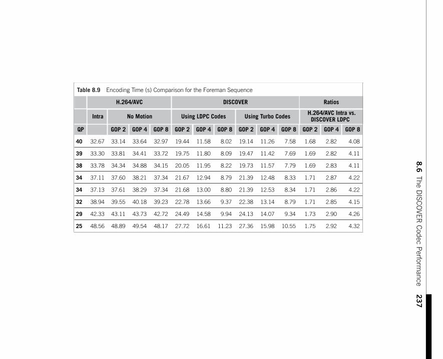
8.6
TheD
ISCO
VERC
odecP
erformance
23
7
Table 8.9 Encoding Time (s) Comparison for the Foreman Sequence
H.264/AVC DISCOVER Ratios
Intra No Motion Using LDPC Codes Using Turbo Codes H.264/AVC Intra vs.DISCOVER LDPC
QP GOP 2 GOP 4 GOP 8 GOP 2 GOP 4 GOP 8 GOP 2 GOP 4 GOP 8 GOP 2 GOP 4 GOP 8
40 32.67 33.14 33.64 32.97 19.44 11.58 8.02 19.14 11.26 7.58 1.68 2.82 4.08
39 33.30 33.81 34.41 33.72 19.75 11.80 8.09 19.47 11.42 7.69 1.69 2.82 4.11
38 33.78 34.34 34.88 34.15 20.05 11.95 8.22 19.73 11.57 7.79 1.69 2.83 4.11
34 37.11 37.60 38.21 37.34 21.67 12.94 8.79 21.39 12.48 8.33 1.71 2.87 4.22
34 37.13 37.61 38.29 37.34 21.68 13.00 8.80 21.39 12.53 8.34 1.71 2.86 4.22
32 38.94 39.55 40.18 39.23 22.78 13.66 9.37 22.38 13.14 8.79 1.71 2.85 4.15
29 42.33 43.11 43.73 42.72 24.49 14.58 9.94 24.13 14.07 9.34 1.73 2.90 4.26
25 48.56 48.89 49.54 48.17 27.72 16.61 11.23 27.36 15.98 10.55 1.75 2.92 4.32
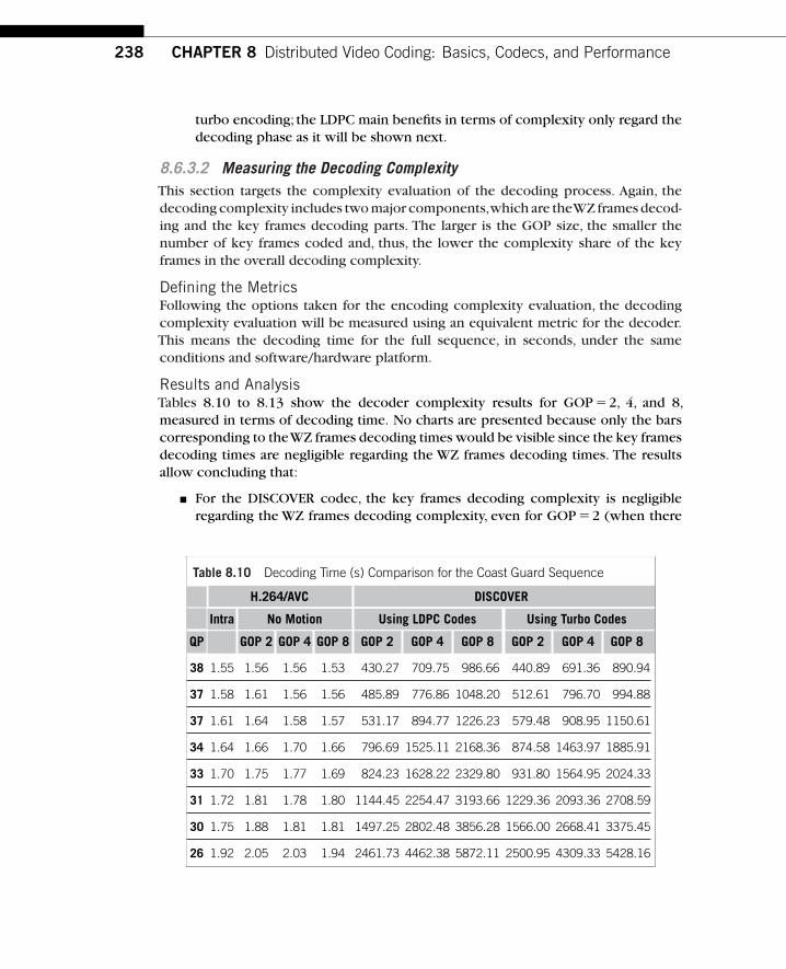
238 CHAPTER 8 Distributed Video Coding: Basics, Codecs, and Performance
turbo encoding; the LDPC main benefits in terms of complexity only regard thedecoding phase as it will be shown next.
8.6.3.2 Measuring the Decoding ComplexityThis section targets the complexity evaluation of the decoding process. Again, thedecoding complexity includes two major components,which are theWZ frames decod-ing and the key frames decoding parts. The larger is the GOP size, the smaller thenumber of key frames coded and, thus, the lower the complexity share of the keyframes in the overall decoding complexity.
Defining the MetricsFollowing the options taken for the encoding complexity evaluation, the decodingcomplexity evaluation will be measured using an equivalent metric for the decoder.This means the decoding time for the full sequence, in seconds, under the sameconditions and software/hardware platform.
Results and AnalysisTables 8.10 to 8.13 show the decoder complexity results for GOP �2, 4, and 8,measured in terms of decoding time. No charts are presented because only the barscorresponding to theWZ frames decoding times would be visible since the key framesdecoding times are negligible regarding the WZ frames decoding times. The resultsallow concluding that:
■ For the DISCOVER codec, the key frames decoding complexity is negligibleregarding the WZ frames decoding complexity, even for GOP �2 (when there
Table 8.10 Decoding Time (s) Comparison for the Coast Guard Sequence
H.264/AVC DISCOVER
Intra No Motion Using LDPC Codes Using Turbo Codes
QP GOP 2 GOP 4 GOP 8 GOP 2 GOP 4 GOP 8 GOP 2 GOP 4 GOP 8
38 1.55 1.56 1.56 1.53 430.27 709.75 986.66 440.89 691.36 890.94
37 1.58 1.61 1.56 1.56 485.89 776.86 1048.20 512.61 796.70 994.88
37 1.61 1.64 1.58 1.57 531.17 894.77 1226.23 579.48 908.95 1150.61
34 1.64 1.66 1.70 1.66 796.69 1525.11 2168.36 874.58 1463.97 1885.91
33 1.70 1.75 1.77 1.69 824.23 1628.22 2329.80 931.80 1564.95 2024.33
31 1.72 1.81 1.78 1.80 1144.45 2254.47 3193.66 1229.36 2093.36 2708.59
30 1.75 1.88 1.81 1.81 1497.25 2802.48 3856.28 1566.00 2668.41 3375.45
26 1.92 2.05 2.03 1.94 2461.73 4462.38 5872.11 2500.95 4309.33 5428.16
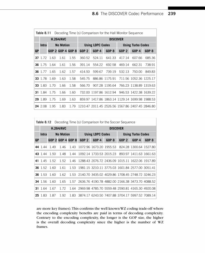
8.6 The DISCOVER Codec Performance 239
Table 8.11 Decoding Time (s) Comparison for the Hall Monitor Sequence
H.264/AVC DISCOVER
Intra No Motion Using LDPC Codes Using Turbo Codes
QP GOP 2 GOP 4 GOP 8 GOP 2 GOP 4 GOP 8 GOP 2 GOP 4 GOP 8
37 1.72 1.63 1.61 1.55 360.52 524.11 641.33 417.14 607.66 685.36
36 1.75 1.64 1.61 1.56 391.14 554.22 692.58 469.14 662.31 738.91
36 1.77 1.65 1.62 1.57 414.50 599.67 739.19 532.13 750.00 849.83
33 1.78 1.69 1.63 1.58 545.75 886.86 1175.91 711.56 1052.36 1225.17
33 1.83 1.70 1.66 1.58 566.70 907.28 1195.64 766.23 1138.89 1319.63
31 1.84 1.75 1.66 1.60 732.00 1197.86 1612.94 946.53 1422.38 1639.22
29 1.89 1.75 1.69 1.63 859.97 1417.86 1863.14 1129.14 1699.98 1988.53
24 2.08 1.95 1.83 1.79 1210.47 2011.45 2526.56 1567.86 2407.45 2846.80
Table 8.12 Decoding Time (s) Comparison for the Soccer Sequence
H.264/AVC DISCOVER
Intra No Motion Using LDPC Codes Using Turbo Codes
QP GOP 2 GOP 4 GOP 8 GOP 2 GOP 4 GOP 8 GOP 2 GOP 4 GOP 8
44 1.44 1.49 1.46 1.43 1072.96 1673.20 1955.53 824.28 1300.64 1527.80
43 1.44 1.50 1.48 1.44 1092.14 1733.53 2015.23 893.97 1411.63 1661.63
41 1.45 1.52 1.52 1.46 1288.43 2076.72 2436.09 1015.11 1622.06 1917.89
36 1.52 1.60 1.61 1.53 1981.15 3210.11 3775.03 1601.84 2577.00 3051.41
36 1.53 1.60 1.62 1.53 2140.70 3435.02 4029.86 1708.45 2748.72 3246.23
34 1.56 1.60 1.65 1.57 2636.76 4190.78 4882.00 2166.38 3473.70 4088.52
31 1.64 1.67 1.72 1.64 2969.98 4785.70 5559.48 2590.81 4165.30 4920.08
25 1.83 1.87 1.92 1.83 3874.17 6243.50 7407.88 3704.17 5997.52 7089.14
are more key frames).This confirms the well known WZ coding trade-off wherethe encoding complexity benefits are paid in terms of decoding complexity.Contrary to the encoding complexity, the longer is the GOP size, the higheris the overall decoding complexity since the higher is the number of WZframes.
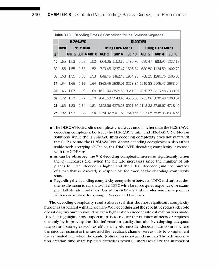
240 CHAPTER 8 Distributed Video Coding: Basics, Codecs, and Performance
Table 8.13 Decoding Time (s) Comparison for the Foreman Sequence
H.264/AVC DISCOVER
Intra No Motion Using LDPC Codes Using Turbo Codes
QP GOP 2 GOP 4 GOP 8 GOP 2 GOP 4 GOP 8 GOP 2 GOP 4 GOP 8
40 1.55 1.53 1.53 1.50 664.06 1150.11 1486.70 590.47 983.92 1237.19
39 1.55 1.55 1.53 1.52 729.45 1237.47 1605.34 680.80 1124.59 1402.70
38 1.58 1.55 1.58 1.53 848.45 1482.45 1904.23 768.25 1280.75 1606.08
34 1.64 1.66 1.66 1.64 1362.45 2536.06 3293.84 1219.88 2105.47 2663.94
34 1.66 1.67 1.69 1.64 1541.00 2824.58 3641.94 1346.77 2319.48 2930.91
32 1.72 1.73 1.77 1.70 2041.53 3640.48 4586.58 1765.06 3030.48 3808.64
29 1.83 1.83 1.84 1.81 2352.56 4273.28 5551.36 2148.23 3738.67 4728.45
25 1.92 1.97 1.98 1.94 3254.92 5901.63 7640.66 3207.05 5535.03 6974.56
■ The DISCOVER decoding complexity is always much higher than the H.264/AVCdecoding complexity, both for the H.264/AVC Intra and H264/AVC No Motionsolutions. While the H.264/AVC Intra decoding complexity does not vary withthe GOP size and the H.264/AVC No Motion decoding complexity is also ratherstable with a varying GOP size, the DISCOVER decoding complexity increaseswith the GOP size.
■ As can be observed, the WZ decoding complexity increases significantly whenthe Qi increases (i.e., when the bit rate increases) since the number of bit-planes to LDPC decode is higher and the LDPC decoder (and the numberof times that is invoked) is responsible for most of the decoding complexityshare.
■ Regarding the decoding complexity comparison between LDPC and turbo codes,the results seem to say that,while LDPC wins for more quiet sequences,for exam-ple, Hall Monitor and Coast Guard for GOP �2, turbo codes win for sequenceswith more motion, for example, Soccer and Foreman.
The decoding complexity results also reveal that the most significant complexityburden is associated with the Slepian–Wolf decoding and the repetitive request-decodeoperation; this burden would be even higher if no encoder rate estimation was made.This fact highlights how important it is to reduce the number of decoder requests,not only by improving the side information quality, but also by adopting adequaterate control strategies such as efficient hybrid encoder-decoder rate control wherethe encoder estimates the rate and the feedback channel serves only to complementthe estimated rate when the (under)estimation is not good enough.The side informa-tion creation time share typically decreases when Qi increases since the number of

8.7 Final Remarks 241
bit-planes to LDPC decode is higher; on the contrary, the LDPC decoding time shareincreases with Qi when compared to the remaining modules.
8.7 FINAL REMARKSThis chapter has reviewed the state-of-the-art on distributed video coding, going fromthe basics and the first WZ video codecs to the more recent developments repre-sented by the DISCOVER WZ video codec. Although it is difficult to state, at this stage,if any video coding product will ever use distributed source coding (DSC) princi-ples, and for what purpose, it is most interesting to study and research toward thispossibility.
In terms of RD performance, the DISCOVER video codec already wins against theH.264/AVC Intra codec, for most test sequences, and for GOP �2; for more quietsequences, the DISCOVER codec may even win against the H.264/AVC No Motioncodec. For longer GOP sizes, winning against H.264/AVC Intra is more difficult, high-lighting the importance and difficulty of getting good side information, notably whenkey frames are farther away. The feedback channel rate is rather low since a reducednumber of requests are made after the initial encoder rate estimation. However, theuse of a feedback channel adds delay and requires a real-time setup. To address thislimitation, allowing Stanford-based WZ video codecs to be applicable to applicationsthat do not have a feedback channel, for example, storage applications, a WZ videocodec with encoder rate control (without feedback channel) has also been developedin the DISCOVER project [37]. This first feedback channel-free WZ video codec paysa RD performance loss up to 1.2 dB,especially for the highest bit rates, to avoid usageof the feedback channel by using a pure encoder-based rate control.
The DISCOVER encoding complexity is always much lower than the H.264/AVCIntra encoding complexity, even for GOP �2 where it performs better in terms ofRD performance. Since the DISCOVER codec performs better than H.264/AVC Intrafor GOP �2, for most sequences, this highlights that Wyner–Ziv coding is already acredible solution when encoding complexity is a very critical requirement (even ifat the cost of some additional decoding complexity). Good examples of these appli-cations may be deep space video transmission, video surveillance, and video sensornetworks.
Further WZ video coding research should address issues such as side informationcreation, progressive side information refinement, correlation noise modeling, novelchannel codes, rate control, and spatial and temporal adaptive WZ coding. Recentdevelopments have shown thatWZ video coding is still at a rather immature stage com-pared with the level of optimization of the alternative solutions, and thus significantgains can still be obtained for most of the WZ video architecture modules.
It is presently more and more accepted that DSC principles are leading to a variety oftools that may help to solve different problems,not only coding but also,authentication,tampering detection [53], and secure biometrics [54]. The future will tell in whichapplication domains distributed source coding principles will find success.

242 CHAPTER 8 Distributed Video Coding: Basics, Codecs, and Performance
ACKNOWLEDGMENTSMuch of the work presented in this chapter was developed within DISCOVER,a European Project (http://www.discoverdvc.org), and VISNET II, a European Net-work of Excellence (http://www.visnet-noe.org), both funded under the EuropeanCommission IST FP6 program.
The authors would like to acknowledge that the DISCOVER performance resultsincluded in this chapter were the result of a collaborative effort developed by all theDISCOVER partners.
REFERENCES[1] T. Wiegand, G. J. Sullivan, G. Bjontegaard, and A. Luthra, “Overview of the H.264/AVC Video
Coding Standard,” IEEE Trans. on Circuits and Systems for Video Technology, vol. 13, no. 7,pp. 560–576, July 2003.
[2] J. Slepian and J. Wolf, “Noiseless Coding of Correlated Information Sources,” IEEE Trans. onInformation Theory, vol. 19, no. 4, pp. 471–480, July 1973.
[3] A. Wyner and J. Ziv,“The Rate-Distortion Function for Source Coding with Side Information atthe Decoder,” IEEE Trans. on Information Theory, vol. 22, no. 1, pp. 1–10, January 1976.
[4] DISCOVER Page, http://www.img.lx.it.pt/∼discover/home.html
[5] X. Artigas, J. Ascenso, M. Dalai, S. Klomp, D. Kubasov, and M. Ouaret,“The DISCOVER Codec:Architecture, Techniques and Evaluation,” Picture Coding Symposium, Lisbon, Portugal,November 2007.
[6] X. Artigas, S. Malinowski, C. Guillemot, and L. Torres,“Overlapped Quasi-Arithmetic Codes forDistributed Video Coding,” International Conference on Image Processing, San Antonio, TX,September 2007.
[7] A. Wyner,“Recent Results in the Shannon Theory,” IEEE Trans. on Information Theory, vol. 20,no. 1, pp. 2–10, January 1974.
[8] R. Zamir, “The Rate Loss in the Wyner–Ziv Problem,” IEEE Trans. on Information Theory,vol. 42, no. 6, pp. 2073–2084, November 1996.
[9] S. S. Pradhan, J. Chou, and K. Ramchandran, “Duality between Source Coding and ChannelCoding and Its Extension to the Side Information Case,” IEEE Trans. on Information Theory,vol. 49, no. 5, pp. 1181–1203, May 2003.
[10] F. Pereira et al.,“Distributed Video Coding:Selecting the Most Promising Application Scenarios,”Signal Processing: Image Communication, vol. 23, no. 5, pp. 339–352, June 2008.
[11] C. Guillemot, F. Pereira, L. Torres, T. Ebrahimi, R. Leonardi, and J. Ostermann, “DistributedMonoview and Multiview Video Coding,” IEEE Signal Processing Magazine, vol. 24, no. 5,pp. 67–76, September 2007.
[12] A.Aaron,R. Zhang,and B. Girod,“Wyner–Ziv Coding of MotionVideo,” Asilomar Conference onSignals, Systems and Computers, Pacific Grove, CA, November 2002.
[13] A. Aaron, S. Rane, E. Setton, and B. Girod, “Transform-Domain Wyner–Ziv Codec for Video,”Visual Communications and Image Processing, San Jose, CA, January 2004.
[14] B. Girod, A. Aaron, S. Rane, and D. Rebollo-Monedero,“Distributed Video Coding,”Proceedingsof the IEEE, vol. 93, no. 1, pp. 71–83, January 2005.

References 243
[15] R. Puri and K. Ramchandran, “PRISM: A New Robust Video Coding Architecture Based onDistributed Compression Principles,” 40th Allerton Conference on Communication, Control,and Computing, IL, Allerton, October 2002.
[16] R. Puri, A. Majumdar, and K. Ramchandran, “PRISM: A Video Coding Paradigm with MotionEstimation at the Decoder,” IEEE Trans. on Image Processing, vol. 16, no. 10, pp. 2436–2448,October 2007.
[17] S. S. Pradhan and K. Ramchandran, “Distributed Source Coding Using Syndromes (DIS-CUS): Design and Construction,” IEEE Data Compression Conference, Snowbird, UT,pp. 158–167, March 1999.
[18] J. Bajcsy, and P. Mitran, “Coding for the Slepian–Wolf Problem with Turbo Codes,” GlobalCommunication Symposium, San Antonio,TX, pp. 1400–1404, November 2001.
[19] J. Garcia-Frias and Y. Zhao, “Compression of Correlated Binary Sources Using Turbo Codes,”IEEE Communication Letters, vol. 5, pp. 417–419, October 2001.
[20] A. Aaron and B. Girod, “Compression with Side Information Using Turbo Codes,” IEEE DataCompression Conference, Snowbird, UT, April 2002.
[21] A. D. Liveris, Z. Xiong, and C. N. Georghiades,“Compression of Binary Sources with Side Infor-mation at the Decoder Using LDPC Codes,” IEEE Communication Letters, vol. 6, pp. 440–442,October 2002.
[22] D. Varodayan, A. Aaron, and B. Girod, “Rate-Adaptive Codes for Distributed Source Coding,”EURASIP Signal Processing Journal, Special Issue on Distributed Source Coding, vol. 86,no. 11, pp. 3123–3130, November 2006.
[23] Q. Xu, V. Stankovic, and Z. Xiong, “Distributed Joint Source-Channel Coding of Video UsingRaptor Codes,” IEEE Journal on Selected Areas in Communications, vol. 25, no. 4, pp.851–861, May 2007.
[24] D. J. C. MacKay, “Fountain Codes,” IEE Proceedings-Communications, vol. 152, no. 6,pp. 1062–1068, December 2005.
[25] Q. Xu, V. Stankovic, and Z. Xiong, “Wyner–Ziv Video Compression and Fountain Codes forReceiver-Driven Layered Multicast,”IEEE Trans.on Circuits and Systems forVideo Technology,vol. 17, no. 7, pp. 901–906, July 2007.
[26] J.Ascenso,C. Brites,and F. Pereira,“Improving Frame Interpolation with Spatial Motion Smooth-ing for Pixel Domain Distributed Video Coding,” EURASIP Conference on Speech and ImageProcessing, Multimedia Communications and Services, Smolenice, Slovak Republic, June 2005.
[27] J.Ascenso,C. Brites,and F. Pereira,“ContentAdaptiveWyner–Ziv Video Coding Driven by MotionActivity,” International Conference on Image Processing, Atlanta, GA, October 2006.
[28] L. Natário, C. Brites, J. Ascenso, and F. Pereira,“Extrapolating Side Information for Low-DelayPixel-Domain Distributed Video Coding,” International. Workshop on Very Low Bitrate VideoCoding, Sardinia, Italy, September 2005.
[29] D. Varodayan, Y.-C. Lin, A. Mavlankar, M. Flierl, and B. Girod, “Wyner–Ziv Coding of StereoImages with Unsupervised Learning of Disparity,”Picture Coding Symposium,Lisbon,Portugal,November 2007.
[30] C. Brites, J. Ascenso, and F. Pereira,“Modeling Correlation Noise Statistics at Decoder for PixelBased Wyner–Ziv Video Coding,”Picture Coding Symposium, Beijing, China, April 2006.
[31] C. Brites, J. Ascenso, and F. Pereira,“Studying Temporal Correlation Noise Modeling for PixelBased Wyner–Ziv Video Coding,” International Conference on Image Processing, Atlanta, GA,October 2006.
[32] C. Brites and F. Pereira,“Correlation Noise Modeling for Efficient Pixel and Transform DomainWyner–ZivVideo Coding,”IEEE Trans.on Circuits and Systems forVideo Technology, acceptedfor publication.
244 CHAPTER 8 Distributed Video Coding: Basics, Codecs, and Performance
[33] D. Kubasov, J. Nayak, and C. Guillemot,“Optimal Reconstruction in Wyner–Ziv Video Codingwith Multiple Side Information,” IEEE Multimedia Signal Processing Workshop, Chania, Crete,Greece, October 2007.
[34] A. Trapanese, M. Tagliasacchi, S. Tubaro, J. Ascenso, C. Brites, and F. Pereira,“Intra Mode Deci-sion Based on Spatio-Temporal Cues in Pixel Domain Wyner–Ziv Video Coding,” InternationalConference on Acoustics, Speech, and Signal Processing,Toulouse, France, May 2006.
[35] A. Aaron, S. Rane, and B. Girod,“Wyner–Ziv Video Coding with Hash-based Motion Compen-sation at the Receiver,” International Conference on Image Processing, Singapore, October2004.
[36] J. Ascenso and F. Pereira, “Adaptive Hash-based Side Information Exploitation for EfficientWyner–Ziv Video Coding,” International Conference on Image Processing, San Antonio, TX,September 2007.
[37] C. Brites and F. Pereira,“Encoder Rate Control for Transform DomainWyner–ZivVideo Coding,”International Conference on Image Processing, San Antonio,TX, September 2007.
[38] D. Kubasov,K. Lajnef, and C. Guillemot,“A Hybrid Encoder/Decoder Rate Control for a Wyner–Ziv Video Codec with a Feedback Channel,” IEEE Multimedia Signal Processing Workshop,Chania, Crete, Greece, October 2007.
[39] J. D. Areia, J. Ascenso, C. Brites, and F. Pereira,“Low Complexity Hybrid Rate Control for LowerComplexity Wyner–Ziv Video Decoding,” European Signal Processing Conference, Lausanne,Switzerland, August 2008.
[40] M. Tagliasacchi, J. Pedro, F. Pereira, and S. Tubaro,“An Efficient Request Stopping Method at theTurbo Decoder in Distributed Video Coding,” European Signal Processing Conference, Poznan,Poland, September 2007.
[41] S. Shamai, S. Verdú, and R. Zamir,“Systematic Lossy Source/Channel Coding,” IEEE Trans. onInformation Theory, vol. 44, no. 2, pp. 564–579, March 1998.
[42] A. Sehgal, A. Jagmohan, and N. Ahuja, “Wyner–Ziv Coding of Video: An Error-Resilient Com-pression Framework,” IEEE Transactions on Multimedia, vol. 6, no. 2, pp. 249–258, April2004.
[43] S. Rane, P. Baccichet, and B. Girod, “Modeling and Optimization of a Systematic Lossy ErrorProtection System Based on H.264/AVC Redundant Slices,”Picture Coding Symposium,Beijing,China, April 2006.
[44] J. Wang, A. Majumdar, K. Ramchandran, and H. Garudadri, “Robust Video Transmission overa Lossy Network Using a Distributed Source Coded Auxiliary Channel,” Picture CodingSymposium, San Francisco, CA, December 2004.
[45] J. Pedro et al.,“Studying Error Resilience Performance for a Feedback Channel BasedTransformDomain Wyner–Ziv Video Codec,” Picture Coding Symposium, Lisbon, Portugal, November2007.
[46] A. Sehgal, A. Jagmohan, and N. Ahuja,“Scalable Video Coding Using Wyner–Ziv Code,” PictureCoding Symposium, San Francisco, CA, December 2004.
[47] M.Tagliasacchi, A. Majumdar,and K. Ramchandran,“A Distributed Source Coding Based Spatio-Temporal Scalable Video Codec,” Picture Coding Symposium, San Francisco, CA, December2004.
[48] H. Wang, N. Cheung, and A. Ortega,“A Framework for Adaptive Scalable Video Coding UsingWyner–Ziv Techniques,” EURASIP Journal on App. Signal Processing, vol. 2006, Article ID60971.
[49] Q. Xu and Z. Xiong, “Layered Wyner–Ziv Video Coding,” IEEE Trans. on Image Processing,vol. 15, no. 12, pp. 3791–3803, December 2006.
References 245
[50] M. Ouaret, F. Dufaux, and T. Ebrahimi,“Codec-Independent Scalable Distributed Video Coding,”International Conference on Image Processing, San Antonio, TX, September 2007.
[51] J. Ascenso, C. Brites, and F. Pereira, “Design and Performance of a Novel Low-DensityParity-Check Code for Distributed Video Coding,” IEEE International Conference on ImageProcessing, San Diego, CA, October 2008.
[52] F. Pereira, J. Ascenso, and C. Brites, “Studying the GOP Size Impact on the Performance ofa Feedback Channel-based Wyner–Ziv Video Codec,” IEEE Pacific Rim Symposium on ImageVideo and Technology, Santiago, Chile, December 2007.
[53] Y.-C. Lin, D. Varodayan, and B. Girod,“Image Authentication and Tampering Localization UsingDistributed Source Coding,” IEEE Multimedia Signal Processing Workshop, Chania, Crete,Greece, October 2007.
[54] S. C. Draper, A. Khisti,E. Martinian, A.Vetro,and J. S.Yedidia,“Using Distributed Source Codingto Secure Fingerprint Biometrics,” International Conference on Acoustics, Speech, and SignalProcessing, Honolulu, HI, April 2007.

CHAPTER
9Model-based Multiview VideoCompression UsingDistributed Source CodingPrinciples
Jayanth NayakMayachitra, Inc., Santa Barbara, CA
Bi Song, Ertem Tuncel, and Amit K. Roy-ChowdhuryDepartment of Electrical Engineering University of California, Riverside, CA
C H A P T E R C O N T E N T SIntroduction . . . . . . . . . . . . . . . . . . . . . . . . . . . . . . . . . . . . . . . . . . . . . . . . . . . . . . . . . . . . . . . . . . . . . . . . . . . . . . 247Model Tracking. . . . . . . . . . . . . . . . . . . . . . . . . . . . . . . . . . . . . . . . . . . . . . . . . . . . . . . . . . . . . . . . . . . . . . . . . . . 249
Image Appearance Model of a Rigid Object . . . . . . . . . . . . . . . . . . . . . . . . . . . . . . . . . . . . . . . . 250Inverse Compositional Estimation of 3D Motion and Illumination . . . . . . . . . . . . . . . . . 251
Distributed Compression Schemes. . . . . . . . . . . . . . . . . . . . . . . . . . . . . . . . . . . . . . . . . . . . . . . . . . . . . . . 254Feature Extraction and Coding . . . . . . . . . . . . . . . . . . . . . . . . . . . . . . . . . . . . . . . . . . . . . . . . . . . . . 255Types of Frames . . . . . . . . . . . . . . . . . . . . . . . . . . . . . . . . . . . . . . . . . . . . . . . . . . . . . . . . . . . . . . . . . . . . 256Types of Side Information . . . . . . . . . . . . . . . . . . . . . . . . . . . . . . . . . . . . . . . . . . . . . . . . . . . . . . . . . . 257
Experimental Results . . . . . . . . . . . . . . . . . . . . . . . . . . . . . . . . . . . . . . . . . . . . . . . . . . . . . . . . . . . . . . . . . . . . 258Conclusions . . . . . . . . . . . . . . . . . . . . . . . . . . . . . . . . . . . . . . . . . . . . . . . . . . . . . . . . . . . . . . . . . . . . . . . . . . . . . . 263References . . . . . . . . . . . . . . . . . . . . . . . . . . . . . . . . . . . . . . . . . . . . . . . . . . . . . . . . . . . . . . . . . . . . . . . . . . . . . . . 266
9.1 INTRODUCTIONTransmission of video data from multiple sensors over a wireless network requiresan enormous amount of bandwidth and could easily overwhelm the system. How-ever, by exploiting the redundancy between the video data collected by differentcameras, in addition to the inherent temporal and spatial redundancy within each
Distributed Source Coding: Theory, Algorithms, and ApplicationsCopyright © 2008 by Academic Press, Inc. All rights of reproduction in any form reserved. 247

248 CHAPTER 9 Model-based Multiview Video Compression
video sequence,the required bandwidth can be significantly reduced.Well-establishedvideo compression standards, such as MPEG-1, MPEG-2, MPEG-4, H.261, H.263, andH.264, all rely on efficient transform coding of motion-compensated frames, usingthe discrete cosine transform (DCT) or computationally efficient approximationsto it. However, they can only be used in a protocol that encodes the data of eachsensor independently. Such methods would exploit spatial and temporal redundancywithin each video sequence but would completely ignore the redundancy between thesequences.
In this chapter, we develop novel multiterminal, model-based video coding algo-rithms combining distributed source coding (DSC) and computer vision techniques. Inbroad terms,our schemes rely on model-based tracking of individual video sequencescaptured by cameras (which could be located arbitrarily in space), leading to removalof spatial, temporal, and inter-camera redundancies. The presence of the three-dimensional (3D) model provides correspondence between overlapping feature pointsin the different views, provided that the tracking of the individual sequences is accu-rate. The performance of our algorithm depends, most crucially, on the quality oftracking and the coding efficiency of the distributed quantization scheme. The track-ing must result in correspondences between pixels that are maximally correlated,andthe distributed coding must optimally exploit this correlation.
Although DSC was introduced more than three decades ago by Slepian andWolf [17], and underlying ideas as to how it should be practically implemented wereoutlined by Wyner [20], the papers by Zamir and Shamai [25] and Pradhan andRamchandran [13] arguably demonstrated the feasibility of implementing distributedsource codes for the first time. Following the publication of these papers, consider-able effort has been devoted to adapting DSC ideas to application scenarios such asdistributed image and video coding (e.g., [5, 6, 14, 19, 24, 26]), but the results havebeen mixed. The reason is that while distributed processing appears to be a naturalchoice in many scenarios, the conditions necessary for known DSC schemes to per-form well are rarely satisfied, and the more mature non-DSC techniques either easilyoutperform the DSC schemes or the gains of DSC schemes are relatively small. Wemake similar observations in this work. More specifically, the gains we achieve overseparate coding are diminished because it seems that the temporal redundancies aremuch larger than the intercamera ones.The exception is at very low rates where evensmall gains become significant. In this chapter, we therefore focus on very low bitrates.
Although early work on distributed video coding focused on the single-view case,some attention has been given to applying distributed coding for multiview video aswell [1, 7, 12, 18]. Most of this work has been on block-based coding, and, as in ourwork,a key issue is construction of side information to optimally exploit intrasequencememory and intersequence correlation.
The rest of the chapter is organized as follows. Section 9.2 outlines the model-basedtracking algorithm; Section 9.3 presents an overview of our approach to distributed
9.2 Model Tracking 249
video coding; Section 9.4 gives some experimental results; and finally, Section 9.5presents the conclusion and discusses some avenues for future research.
9.2 MODEL TRACKINGNumerous methods exist for estimating the motion and shape of an object from videosequences. Many of these methods can handle significant changes in the illuminationconditions by compensating for the variations [4, 8, 9]. However, few methods canrecover the 3D motion and time-varying global illumination conditions from videosequences of moving objects.We achieve this goal by building on a recently proposedframework for combining the effects of motion, illumination, 3D shape, and cameraparameters in a sequence of images obtained by a perspective camera [21, 22]. Thistheory allows us to develop a simple method for estimating the rigid 3D motion,as presented in [21]. However, this algorithm involves the computation of a bilinearbasis (see Section 9.2.1) in each iteration, which is a huge computational burden.In this chapter, we show that it is possible to efficiently and accurately reconstructthe 3D motion and global lighting parameters of a rigid and nonrigid object from avideo sequence within the framework of the inverse compositional (IC) algorithm [2].Details of this approach are available in [23].
A well-known approach for 2D motion estimation and registration in monocularsequences is Lucas–Kanade tracking, which attempts to match a target image witha reference image or template. Building on this framework, a very efficient trackingalgorithm was proposed in [8] by inverting the role of the target image and the tem-plate. However,this algorithm can only be applied to restricted class of warps betweenthe target and template (for details, see [2]). A forward compositional algorithm wasproposed in [16] by estimating an incremental warp for image alignment. Baker andMatthews [2] proposed an IC algorithm for efficient implementation of the Lucas–Kanade algorithm to save computational cost in reevaluation of the derivatives ineach iteration.The IC algorithm was then used for efficiently fitting active appearancemodels [11] and the well-known 3D morphable model (3DMM) [15] to face imagesunder large pose variations. However, none of these schemes estimates the lightingconditions in the images. A version of 3DMM fitting [3] used a Phong illuminationmodel,estimation of whose parameters in the presence of extended light sources canbe difficult.
Our lighting estimation can account for extended lighting sources and attachedshadows. Furthermore, our goal is to estimate 3D motion, unlike in [4, 8, 16], worksthat perform 2D motion estimation. The warping function in the present work isdifferent from [2,15], as we explain in Section 9.2.2. Since our IC approach estimates3D motion, it allows us to perform the expensive computations only once every fewframes (unlike once for every frame as in the image alignment approaches of Baker
250 CHAPTER 9 Model-based Multiview Video Compression
and Matthews [2]). Specifically, these computations are done only when there is asignificant change of pose.
9.2.1 Image Appearance Model of a Rigid Object
Our goal is to describe the appearance of an image in terms of the 3D rigid motionand the overall lighting in the scene. For this purpose, we derive a generative imageappearance model that is a function of these parameters. Given a sequence of images,we can estimate the parameters that lead to the best fit with this model. Details of thegenerative model,as well as the estimation framework,are available in [21,22].A briefoverview is provided here.
In [21], it was proved that if the motion of the object (defined as the translationof the object centroid �T∈R
3�1 and the rotation vector ��∈R3�1 about the cen-
troid in the camera frame) from time t1 to new time instance t2 � t1 ��t is small,then up to a first-order approximation, the reflectance image I(x, y) at t2 can beexpressed as
It2(v)�
9∑i�1
lt2i bt2i (v) (9.1)
where
bt2i (v)�bt1
i (v)�A(v, n)�T�B(v, n)��.
In these equations, v represents the image point projected from the 3D surface withsurface normal n, and bt1
i (v) are the original basis images before motion (precise
format of bt1i (v) is defined in [21]). lt �
[lt1 . . . ltNl
]Tis the vector of illumination param-
eters. A and B contain the structure and camera intrinsic parameters,and are functionsof v and the 3D surface normal n. For each pixel v, both A and B are Nl �3 matrices,where Nl≈9 for Lambertian objects with attached shadows. A derivation of (9.1) andexplicit expressions for A and B are presented in [21]. For the purposes of this chapter,we only need to know the form of the equations.
The left side of Equation (9.1) is the image at time t2,which is expressed in terms ofthe basis images and the lighting coefficients on the right-hand side.The basis images,in turn, depend on the motion of the object between two consecutive time instants.Thus,Equation (9.1) expresses the image appearance in terms of the object’s 3D poseand the scene lighting.
We can express the result in (9.1) succinctly using tensor notation as
It2 �
(Bt1 �Ct1 �2
[�T��
])�1 lt2 , (9.2)
where �n is called the mode-n product [10] and l∈RNl is the Nl -dimensional
vector of li components. More specifically, the mode-n product of a tensor
9.2 Model Tracking 251
A∈RI1�I2�...�In�...�IN by a vector V∈R
In�1, denoted by A�n V, is the I1 � I2 � . . .
� 1 � . . .� IN tensor
(A�n V)i1...in�11in�1...iN �∑in
ai1...in�1inin�1...iN vin .
Thus,the image at t2 can be represented using the parameters computed at t1. For eachpixel (p, q) in the image,Cpq �
[A B
]of size Nl �6.Thus for an image of size M �N ,
C is Nl �6�M �N , Bt1 is a subtensor of dimension Nl �1�M �N , comprising thebasis images bt1
i (u), and It2 is a subtensor of dimension 1�1�M �N , representingthe image.
9.2.2 Inverse Compositional Estimation of 3D Motion and Illumination
We now present the estimation algorithm for the bilinear model in Equation (9.2).Thedetailed proof of convergence and extension to video for the rigid motion case canbe found in [23].
We begin by estimating the 3D motion assuming that illumination is constant acrosstwo consecutive frames.We will then estimate variations in illumination. Let p∈R
6�1
denote the pose of the object.Then the image synthesis process can be considered as arendering function of the object at pose p in the camera frame to the pixel coordinatesv in the image plane as f (v, p). Using the bilinear model described above, it can beimplemented with Equation (9.2). Given an input image I(v), we want to align thesynthesized image with it so as to obtain
p�arg minp
∑v
(f (v, p)� I(v)
)2, (9.3)
where p denotes the estimated pose for this input image I(v).This is the cost functionof Lucas–Kanade tracking in [2] modified for 3D motion estimation.
We will consider the problem of estimating the pose change, mt ��pt , betweentwo consecutive frames, It(v) and It�1(v). Let us introduce a warp operator W :R2→R
2 such that, if we denote the pose of It(v) as p, the pose of It(Wp(v,�p)) is p��p(see Figure 9.1). Specifically, a 2D point on the image plane is projected onto the 3Dobject surface. Then we transform the pose of the object surface by �p and back-project the point from the 3D surface onto the image plane. Thus, Wp represents thedisplacement in the image plane due to a pose transformation of the 3D model. Notethat this warping involves a 3D pose transformation (unlike [2]). In [15], the warp-ing was from a point on the 3D surface to the image plane and was used for fittinga 3D model to an image. Our new warping function can be used for the IC estima-tion of 3D rigid motion and illumination in video sequence, which [2] and [15] donot address.
A key property of {Wp} is that these warps form a group with respect to functioncomposition (see [23] for a detailed proof of this and other properties of the set ofwarps), which is necessary for applying the IC algorithm. Here we will only showhow the inverse of a warp is another warp. The inverse of the warp W is defined

252 CHAPTER 9 Model-based Multiview Video Compression
Pose p 1 Dp
3D Model
u
v
v
WD
Pose p It (v)I(Wc(v, Dp), t )
FIGURE 9.1
Illustration of the warping function W. A point v in image plane is projected onto the surface of the3D object model. After the pose transformation with �p, the point on the surface is backprojectedonto the image plane at a new point u. The warping function maps from v∈R
2 to u∈R2. The red
ellipses show the common part in both frames upon which the warping function W is defined.
to be the R2→R
2 mapping such that if we denote the pose of It(v) as p, the poseof It(Wp(Wp(v,�p),�p)�1) is p itself. As the warp Wp(v,�p) transforms the posefrom p to p��p, the inverse Wp(v,�p)�1 should transform the pose from p��pto p, that is, Wp(v,�p)�1 �Wp��p(v, ��p).
Using this warp operator, for any frame It(v), we can write the cost function as
mt �arg minm
∑v
(f (v, pt�1)� It(Wpt�1(v, �m))
)2. (9.4)
Rewriting the cost function (9.4) in the IC framework [2], we consider minimizing
arg min�m
∑v
(f (Wpt�1
(v,�m), pt�1
)� It(Wpt�1(v, �m)))2
(9.5)
with the update rule
Wpt�1(v, �m)←Wpt�1(v, �m)◦Wpt�1(v,�m)�1. (9.6)
The compositional operator ◦ in Equation (9.6) means the second warp is com-posed into the first warp, that is, Wpt�1(v, �m)≡Wpt�1(Wpt�1(v,�m)�1, �m).
According to the definition of the warp W, we can replace f (Wpt�1(v,�m), p
t�1)
9.2 Model Tracking 253
in (9.5) with f (v, pt�1 ��m). This is because f (v, pt�1 ��m) is the image synthe-sized at pt�1 ��m, while f (Wpt�1
(v,�m), pt�1
) is the image synthesized at pt�1
followed with the warp of the pose increments �m. Applying the first-order Taylorexpansion on it, we have∑
v
(f (v, pt�1)�
�f (v, p)
�p|p�pt�1�m � It(Wpt�1(v, �m))
)2
.
Taking the derivative of the above expression with respect to �m and setting it to bezero, we have∑
v
(f (v, pt�1)�GT
v|pt�1�m � It(Wpt�1(v, �m))
)Gv|pt�1
�0,
where Gv|pt�1is the derivative �f (v,p)
�p |p�pt�1. Solving for �m, we get:
�m �HIC
∑v
Gv|pt�1
(It(Wpt�1
(v, �m))
� f(v, pt�1
))(9.7)
where
HIC �
[∑v
Gv|pt�1GT
v|pt�1
]�1
.
Note that the derivative Gv|pt�1and Hessian HIC in (9.7) do not depend on the updating
variable m,which is moved into the warp operator W.The computational complexityof Wpt�1
(v, �m) will be significantly lower than that of recomputing Gv|pt�1�m andthe corresponding Hessian H in every iteration.
Reintroducing the illumination variation,the lighting parameter l can be estimatedusing
l �(Bl(l)BTl(l))
�1Bl(l)IT(l),
where the subscript (l) indicates the unfolding operation [10] along the illumina-tion dimension. That is, assuming an Nth-order tensor A∈R
I1�I2�...�IN ,the matrix unfolding A(n)∈R
In�(In�1In�2...IN I1I2...In�1) contains the elementai1i2...iN at the position with row number in and column number equal to(in�1 �1) In�2 In�3 . . . IN I1I2 . . . In�1 �(in�2 �1) In�3 In�4 . . . IN I1 I2 . . . In�1 � · · ·�(iN �1)I1I2 . . . In�1 �(i1 �1)I2I3 . . . In�1 � · · ·� in�1.
Following the same derivation as (9.7), we have
�m �HIC
∑v
(Cv|pt�1�1 l)
(It(Wpt�1(v, �m))�Bv|pt�1 �1 l
)(9.8)
where
HIC �
[∑v
(Cv|pt�1�1 l)(Cv|pt�1
�1 l)T
]�1
.

254 CHAPTER 9 Model-based Multiview Video Compression
9.3 DISTRIBUTED COMPRESSION SCHEMESThe distributed compression schemes discussed in this section can all be representedby the block diagram of Figure 9.2. The choices we make for the following blocksresult in the various schemes as described later in this section.
■ Feature extraction■ Mode decision■ Side information extraction
FeatureExtraction
IE PE DE
ModeDecision
ID IDPD PDDD
PredictorExtract SideInformation
FeatureExtraction
ModeDecision
Predictor
IL IR
EstimatePose
EstimatePose
IL IR
DECODER
ENCODER L ENCODER R
DE PE IE
DD
FIGURE 9.2
Block diagram of coding schemes.

9.3 Distributed Compression Schemes 255
9.3.1 Feature Extraction and Coding
In order to extract the image features, we need to detect them in the first frame andtrack them in subsequent frames. Since we estimate a 3D pose,a 3D mesh model is reg-istered to the first frame and then tracked using the method in Section 9.2. The meshmodel consists of a set of mesh points V �{Vi �(xi, yi, zi), i �1, . . . , N } and a set oftriangles T �{Tabc �(Va, Vb, Vb)}⊂V3 formed by mesh points. Figure 9.3 depicts the2D projection of a triangular mesh model on a pair of frames.The model pose param-eters,namely, the translation and rotation parameters, are computed independently ateach view and transmitted to the decoder at high fidelity. Each encoder also receivesthe initial pose parameters of the other encoder.
The visibility of a mesh point V in both views is computed at each encoder bycomputing its position relative to each triangle T �(V1, V2, V3) of which it is not amember. Given the estimated pose of a certain view, let (x, y, z) and (xi, yi, zi) be thecoordinates of V and Vi , respectively. The triangle, which is the convex hull of thethree points, occludes V if the segment connecting the origin to V passes throughthe triangle. To test occlusion, we project the point onto the basis formed by thevertices of T : ⎡⎢⎣cx
cy
cz
⎤⎥⎦�
⎡⎢⎣x1 x2 x3
y1 y2 y3
z1 z2 z3
⎤⎥⎦�1⎡⎢⎣x
y
z
⎤⎥⎦ (9.9)
The triangle occludes the point if and only if cx, cy,and cz are all positive and cx �cy �cz �1. Observe that if all coefficients are positive and sum to 1, the point lies in theconvex hull of the three points forming T , that is, it lies on the triangle. If the meshpoint is visible with respect to every triangle, we declare the point visible.
FIGURE 9.3
Mesh points V and triangles T are overlaid on the two views.

256 CHAPTER 9 Model-based Multiview Video Compression
We consider three feature extraction techniques.
■ Point Sampled Intensity (PSI): The feature set for an image is the set of intensityvalues at the visible mesh points projected onto the image plane.
■ Triangles with Constant Intensity (TCI): For all triangles containing at least onevisible vertex, this feature is the average of the intensity values over the visiblepixels in the triangle.
■ Triangles with Linearly Varying Intensity (TLI): For triangles with all verticesvisible,we compute a linear least squares fit to the intensity profile.The intensityvalues at the vertices according to the estimated planar intensity profile form apart of the feature set. For those triangles where not all vertices are visible, weuse the average intensity feature as in TCI.
For distributed encoding of the extracted features,we utilized a very simple binningtechnique whereby each feature is independently encoded using
C(i)� i mod W
where C(i) is the codeword corresponding to the quantization index i of the codedfeature and W is a parameter controlling the rate of the code. Even though the abovebinning scheme can be improved by more sophisticated DSC techniques (e.g., LDPC-or turbo-based codes) in general, the improvement would be marginal at very low bitrates, which we particularly focus on.
9.3.2 Types of Frames
In the compression schemes that we consider,each frame of each view can belong toone of three classes:
■ Intraframe or I-frame: Each feature is encoded and decoded independently ofboth past frames in the same view and all frames in the other view.
■ Predictive frame or P-frame: If any feature is common to the current frame andthe previous frame in the same view, we only encode the difference betweenthe two features. Features that are unique to the current frame are coded as inan I-frame.
■ Distributed frame or D-frame:The features for which side information is availableat the decoder are distributively coded, while the rest of the features are codedas in an I-frame.
We considered two schemes for coding sequences:
■ Scheme 1: We begin with an I-frame in both views. For the subsequentDRefreshPeriod-1 sampling instants, both views are coded as P-frames. At the fol-lowing instant, the left view is transmitted as an I-frame and the other view istransmitted as a D-frame. The next DRefreshPeriod-1 are transmitted as P-frames.For the next instant, the right view is an I-frame while the left is a D-frame.

9.3 Distributed Compression Schemes 257
Table 9.1 Frame Types of Right and Left Views in the TwoSchemes and Separate Coding. (DRefreshPeriod = 3 andIRefreshPeriod = 9)
Frame Number 1 2 3 4 5 6 7 8 9 10
Scheme 1 Left I P P I P P D P P I
Right I P P D P P I P P I
Scheme 2 Left I P P D D D I P P I
Right I D D I P P D D D I
Separate Left I P P I P P I P P I
Right I P P I P P I P P I
This process then repeats. Every IRefreshPeriod instants,both views are coded asI-frames.
■ Scheme 2:As in Scheme 1, we begin with I-frames in both views. For the sub-sequent DRefreshPeriod-1 sampling instants, the left view is coded as a P-frame,while the other view is coded as a D-frame. At the next instant, the right viewis coded as an I-frame, and the other view is coded as a D-frame. This processis repeated in every block of DRefreshPeriod frame pairs with the roles of theright and left views reversing from block to block. Again, as in Scheme 1, everyIRefreshPeriod instants, both views are coded as I-frames.
Table 9.1 shows some representative code sequences.
9.3.3 Types of Side Information
The side information in a D-frame can be one of three types:
■ Other view (OD):The corresponding features between the frame being encodedand the one that is observed at the current instant at the other view form theside information. We can only encode features that are common to both views.
■ Previous frame (PD): We use the corresponding features in the previous framefrom the same view as side information. We can only encode features that arepresent in the previous and current views.
■ Previous frame and Other view (POD):The side information is the optimal linearestimate of the source given the previous frame in the same view and the currentframe in the other view. Only features that are common to the three framesinvolved can be distributively encoded by this method.The estimation coefficients are to be computed at the decoder before recon-structing a given view. So, if for example, frame Rn is distributively coded, weuse the correlations from decoder reconstructions of Rn�1, Rn�2, and Ln�1 toobtain approximations to the optimal estimation coefficients.

258 CHAPTER 9 Model-based Multiview Video Compression
9.4 EXPERIMENTAL RESULTSIn this section, we evaluate the performance of the various schemes in compress-ing a sequence of a face viewed from two cameras under varying illumination.The face mesh model is assumed to be known to both encoders as well as the
(a) (b)
FIGURE 9.4
(a) Five consecutive frames from the original sequence. (b) Separate coding of the two viewsusing the PSI technique and Scheme 1. The bit rate is ≈20 kbps and the PSNR is ≈16.5 dB.

9.4 Experimental Results 259
(a) (b)
FIGURE 9.5
Distributed coding of the sequence using the PSI technique for feature extraction and POD-typeside information. (a) Reconstruction using Scheme 1 with bit rate ≈22 kbps and PSNR ≈21 dB.(b) Reconstruction using Scheme 2 with bit rate ≈18 kbps and PSNR ≈22.8 dB.
decoder. Transmission of the initial model pose parameters forms the sole interencodercommunication.
For both schemes and all feature and side information types, we tested the perfor-mance on a 15-frame sequence from each view. Five consecutive original frames areshown in Figure 9.4(a). We fixed DRefreshPeriod = 5 and IRefreshPeriod = 15.

260 CHAPTER 9 Model-based Multiview Video Compression
10 15 20 25 30 35 40 4513
14
15
16
17
18
19
20
21
22
23
Performance of PSI from frame 1 to frame 15
Rate (kbps)
PS
NR
(dB
)
Scheme 1, ODScheme 1, PDScheme 1, PODSeparateScheme 2, ODScheme 2, PDScheme 2, POD
FIGURE 9.6
The rate-distortion trade-off using the PSI feature extraction technique.
In Figures 9.4(b), 9.5(a), and 9.5(b), examples of reconstructed sequences areshown, respectively, for separate coding, Scheme 1, and Scheme 2, all using the PSItechnique for feature extraction, and the latter two using POD-type side informa-tion. The bit rates are fixed at around 20 kbps. The complete rate-distortion trade-offobtained by running all methods with various parameters is shown in Figure 9.6,whereit is clearly seen that the gains are more significant at lower bit rates.
We then increase the target bit rate to around 41 kbps by adopting the TCI tech-nique for feature extraction. The reason for the rate increase even with the samequantization parameters is that the number of triangles is about twice as large asthe number of mesh points. As apparently seen from the reconstructed sequencesshown in Figures 9.7 and 9.8, this results in a quality increase. That is because theaverage of intensity values within a triangle is a much better representative of thetriangle than a reconstruction based on only the three corner values. However, as canbe seen from the complete rate-distortion trade-off shown in Figure 9.9, the increasein the reconstruction quality comes at the expense of reduced distributed codinggains.
Using the TLI technique for feature extraction, we further increase the bit rateapproximately by a factor of 3, since most triangles are now represented by threeparameters.The reconstructed sequences are shown in Figures 9.10 and 9.11,and the

9.4 Experimental Results 261
(a) (b)
FIGURE 9.7
Coding using the TCI technique for feature extraction. (a) Separate coding of the two views usingScheme 1 with bit rate ≈41 kbps and PSNR ≈23.9 dB. (b) Distributed coding using Scheme 2and PD-type side information with the same bit rate PSNR ≈25.5 dB.
complete rate-distortion trade-off is depicted in Figure 9.12. The distributed codinggains are further diminished in this regime.
Even though PD-type side information yields the best performance at low bitrates as seen from Figures 9.6, 9.9, and 9.12, reconstruction based on POD-type side

262 CHAPTER 9 Model-based Multiview Video Compression
(a) (b)
FIGURE 9.8
Coding using the TCI technique for feature extraction and POD-type side information. (a) Dis-tributed coding using Scheme 1 with bit rate ≈40 kbps and PSNR ≈24.4 dB. (b) Distributedcoding using Scheme 2 with bit rate ≈43 kbps and the same PSNR.
information is more beneficial in scenarios in which the channel carrying the D-frameis less reliable and can result in a very noisy reference for the future D-frames. Onthe other hand, since the temporal correlation is much higher than the correlationbetween the views,relying solely on the other view always yields worse performance.
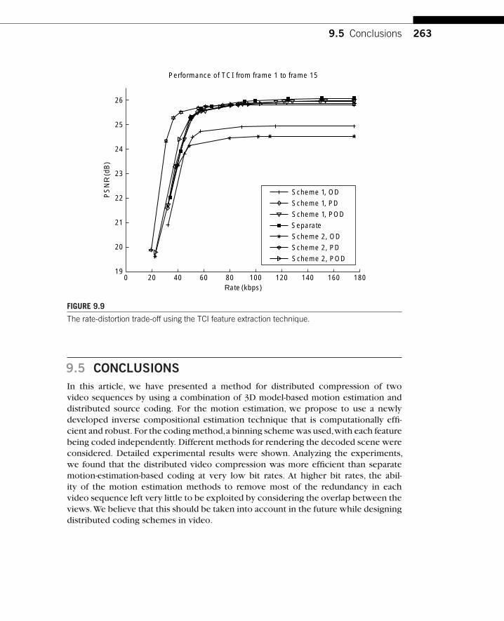
9.5 Conclusions 263
Performance of TCI from frame 1 to frame 15
Rate (kbps)
PS
NR
(dB
)
Scheme 1, OD
Scheme 1, PD
Scheme 1, POD
Separate
Scheme 2, OD
Scheme 2, PD
Scheme 2, POD
0 20 40 60 80 100 120 140 160 18019
20
21
22
23
24
25
26
FIGURE 9.9
The rate-distortion trade-off using the TCI feature extraction technique.
9.5 CONCLUSIONSIn this article, we have presented a method for distributed compression of twovideo sequences by using a combination of 3D model-based motion estimation anddistributed source coding. For the motion estimation, we propose to use a newlydeveloped inverse compositional estimation technique that is computationally effi-cient and robust. For the coding method,a binning scheme was used,with each featurebeing coded independently. Different methods for rendering the decoded scene wereconsidered. Detailed experimental results were shown. Analyzing the experiments,we found that the distributed video compression was more efficient than separatemotion-estimation-based coding at very low bit rates. At higher bit rates, the abil-ity of the motion estimation methods to remove most of the redundancy in eachvideo sequence left very little to be exploited by considering the overlap between theviews.We believe that this should be taken into account in the future while designingdistributed coding schemes in video.

264 CHAPTER 9 Model-based Multiview Video Compression
(a) (b)
FIGURE 9.10
Coding using the TLI technique for feature extraction. (a) Separate coding of the two views usingScheme 1 with bit rate ≈ 120 kbps and PSNR ≈28 dB. (b) Distributed coding using Scheme 1and OD-type side information with bit rate ≈128 kbps and PSNR ≈27 dB.
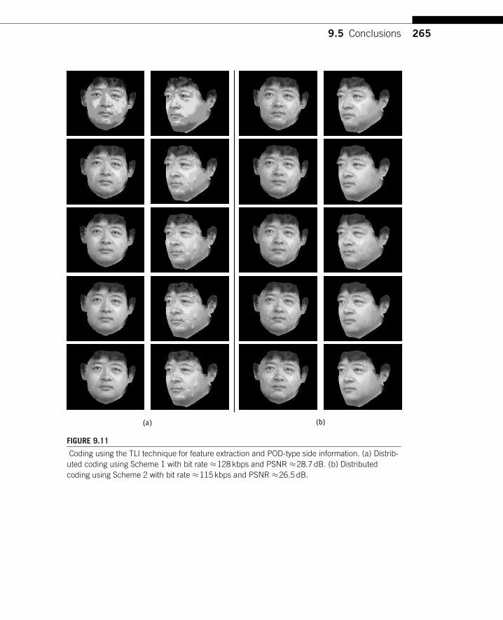
9.5 Conclusions 265
(a) (b)
FIGURE 9.11
Coding using the TLI technique for feature extraction and POD-type side information. (a) Distrib-uted coding using Scheme 1 with bit rate ≈128 kbps and PSNR ≈28.7 dB. (b) Distributedcoding using Scheme 2 with bit rate ≈115 kbps and PSNR ≈26.5 dB.
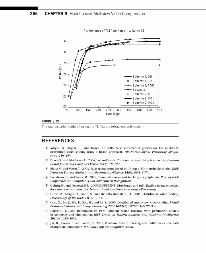
266 CHAPTER 9 Model-based Multiview Video Compression
Performance of TLI from frame 1 to frame 15
Rate (kbps)
PS
NR
(dB
)
Scheme 1, ODScheme 1, PD
Scheme 1, PODSeparateScheme 2, ODScheme 2, PDScheme 2, POD
50 100 150 200 250 300 350 400 450 50020
22
24
26
28
30
32
FIGURE 9.12
The rate-distortion trade-off using the TLI feature extraction technique.
REFERENCES[1] Artigas, X., Angeli, E., and Torres, L.: 2006, Side information generation for multiview
distributed video coding using a fusion approach, 7th Nordic Signal Processing Sympo-sium, 250–253.
[2] Baker, S., and Matthews, I.: 2004, Lucas–Kanade 20 years on: A unifying framework, Interna-tional Journal of Computer Vision 56(3), 221–255.
[3] Blanz, V., and Vetter,T.: 2003, Face recognition based on fitting a 3D morphable model, IEEETrans. on Pattern Analysis and Machine Intelligence 25(9), 1063–1074.
[4] Freedman, D., and Turek, M.: 2005, Illumination-invariant tracking via graph cuts, Proc. of IEEEConference on Computer Vision and Pattern Recognition.
[5] Gehrig, N., and Dragotti, P. L.: 2005, DIFFERENT: Distributed and fully flexible image encodersfor camera sensor networks, International Conference on Image Processing.
[6] Girod, B., Margot, A., Rane, S., and Rebollo-Monedero, D.: 2005, Distributed video coding,Proceedings of the IEEE 93(1), 71–83.
[7] Guo, X., Lu, Y., Wu, F., Gao, W., and Li, S.: 2006, Distributed multi-view video coding, VisualCommunications and Image Processing 2006 6077(1), 60770T.1–60770T.8.
[8] Hager, G. D., and Belhumeur, P.: 1998, Efficient region tracking with parametric modelsof geometry and illumination, IEEE Trans. on Pattern Analysis and Machine Intelligence20(10), 1025–1039.
[9] Jin, H., Favaro, P., and Soatto, S.: 2001, Real-time feature tracking and outlier rejection withchanges in illumination, IEEE Intl. Conf. on Computer Vision.

References 267
[10] Lathauwer, L. D., Moor, B. D., and Vandewalle, J.: 2000,A multilinear singular value decompo-sition, SIAM J. Matrix Anal. Appl.21(4), 1253–1278.
[11] Matthews, I., and Baker, S.: 2004,Active appearance models revisited, International Journal ofComputer Vision 60(2), 135–164.
[12] Ouaret, M., Dufaux, F., and Ebrahimi, T.: 2006, Fusion-based multiview distributed videocoding, 4th ACM International Workshop on Video Surveillance and Sensor Networks,139–144.
[13] Pradhan, S., and Ramchandran, K.: 1999, Distributed source coding using syndromes (DISCUS):Design and construction, Data Compression Conference, 158–167.
[14] Puri, R., and Ramchandran, K.: 2007, PRISM:A video coding architecture based on distributedcompression principles, IEEE Transactions on Image Processing 16(10), 2436–2448.
[15] Romdhani, S., and Vetter, T.: 2003, Efficient, robust and accurate fitting of a 3D morphablemodel, IEEE International Conference on Computer Vision 2003.
[16] Shum, H.-Y., and Szeliski, R.: 2000, Construction of panoramic image mosaics with global andlocal alignment, International Journal of Computer Vision 16(1), 63–84.
[17] Slepian, D., and Wolf, J. K.: 1973, Noiseless coding of correlated information sources, IEEETransactions on Information Theory 19(4), 471–480.
[18] Song, B., Bursalioglu, O., Roy-Chowdhury, A., and Tuncel, E.: 2006, Towards a multi-terminalvideo compression algorithm using epipolar geometry, IEEE Intl. Conf. on Acoustics, Speechand Signal Processing.
[19] Wagner, R., Nowak, R., and Baranuik, R.: 2003, Distributed image compression for sensornetworks using correspondence analysis and superresolution, ICIP, vol. 1: pp. 597–600.
[20] Wyner, A.: 1974, Recent results in the Shannon theory, IEEE Transactions on InformationTheory 20(1), 2–10.
[21] Xu, Y., and Roy-Chowdhury, A.: 2007, Integrating motion, illumination and structure invideo sequences, with applications in illumination-invariant tracking, IEEE Trans. on PatternAnalysis and Machine Intelligence 29(5), 793–807.
[22] Xu, Y., and Roy-Chowdhury, A.: 2008, A Theoretical analysis of linear and multi-linear mod-els of image appearance, IEEE International Conference on Computer Vision and PatternRecognition.
[23] Xu, Y., and Roy-Chowdhury, A.: 2008, Inverse compositional estimation of 3d motion andlighting in dynamic scenes, IEEE Trans. on Pattern Analysis and Machine Intelligence,vol. 30, no. 7, pp. 1300–1307, July 2008.
[24] Yang, Y., Stankovic, V., Zhao, W., and Xiong, Z.: 2007, Multiterminal video coding, IEEEInternational Conference on Image Processing, pp. III 28–28.
[25] Zamir, R., and Shamai, S.: 1998, Nested linear/lattice codes for Wyner–Ziv encoding, Informa-tion Theory Workshop, pp. 92–93.
[26] Zhu, X.,Aaron,A., and Girod, B.: 2003, Distributed compression for large camera arrays, IEEEWorkshop on Statistical Signal Processing.

CHAPTER
10Distributed Compression ofHyperspectral Imagery
Ngai-Man Cheung and Antonio OrtegaSignal and Image Processing Institute, Department of Electrical Engineering,
University of Southern California, Los Angeles, CA
C H A P T E R C O N T E N T SIntroduction . . . . . . . . . . . . . . . . . . . . . . . . . . . . . . . . . . . . . . . . . . . . . . . . . . . . . . . . . . . . . . . . . . . . . . . . . . . . . . 269
Hyperspectral Imagery Compression: State of the Art. . . . . . . . . . . . . . . . . . . . . . . . . . . . . . 271Outline of This Chapter . . . . . . . . . . . . . . . . . . . . . . . . . . . . . . . . . . . . . . . . . . . . . . . . . . . . . . . . . . . . 273
Hyperspectral Image Compression . . . . . . . . . . . . . . . . . . . . . . . . . . . . . . . . . . . . . . . . . . . . . . . . . . . . . . . 273Dataset Characteristics. . . . . . . . . . . . . . . . . . . . . . . . . . . . . . . . . . . . . . . . . . . . . . . . . . . . . . . . . . . . . 273Intraband Redundancy and Cross-band Correlation . . . . . . . . . . . . . . . . . . . . . . . . . . . . . . . . 274Limitations of Existing Hyperspectral Compression Techniques . . . . . . . . . . . . . . . . . . . 275
DSC-based Hyperspectral Image Compression. . . . . . . . . . . . . . . . . . . . . . . . . . . . . . . . . . . . . . . . . . . 277Potential Advantages of DSC-based Hyperspectral Compression . . . . . . . . . . . . . . . . . . 278Challenges in Applying DSC for Hyperspectral Imaging. . . . . . . . . . . . . . . . . . . . . . . . . . . . 279
Example Designs . . . . . . . . . . . . . . . . . . . . . . . . . . . . . . . . . . . . . . . . . . . . . . . . . . . . . . . . . . . . . . . . . . . . . . . . . 280DSC Techniques for Lossless Compression of Hyperspectral Images . . . . . . . . . . . . . . 280Wavelet-based Slepian–Wolf Coding for Lossy-to-lossless Compression ofHyperspectral Images . . . . . . . . . . . . . . . . . . . . . . . . . . . . . . . . . . . . . . . . . . . . . . . . . . . . . . . . . . . . . . 283Distributed Compression of Multispectral Images Using a SetTheoretic Approach . . . . . . . . . . . . . . . . . . . . . . . . . . . . . . . . . . . . . . . . . . . . . . . . . . . . . . . . . . . . . . . . 288
Conclusions . . . . . . . . . . . . . . . . . . . . . . . . . . . . . . . . . . . . . . . . . . . . . . . . . . . . . . . . . . . . . . . . . . . . . . . . . . . . . . 289References . . . . . . . . . . . . . . . . . . . . . . . . . . . . . . . . . . . . . . . . . . . . . . . . . . . . . . . . . . . . . . . . . . . . . . . . . . . . . . . 289
10.1 INTRODUCTIONHyperspectral images are volumetric image cubes that consist of hundreds of spa-tial images. Each spatial image, or spectral band, captures the responses of groundobjects at a particular wavelength (Figure 10.1). For example, the NASA AVIRIS(Airborne Visible/Infrared Imaging Spectrometer) measures the spectral responses in
Distributed Source Coding: Theory, Algorithms, and ApplicationsCopyright © 2008 by Academic Press, Inc. All rights of reproduction in any form reserved. 269

270 CHAPTER 10 Distributed Compression of Hyperspectral Imagery
Wavelength
Relative brightness
FIGURE 10.1
Hyperspectral image.
Table 10.1 Examples of Research and Commercial Imaging Spectrometers [45]
Sensor Organization Country Number of Bands Wavelength Range (�m)
AVIRIS NASA United States 224 0.4–2.5
AISA Spectral Imaging Ltd. Finland 286 0.45–0.9
CASI Itres Research Canada 288 0.43–0.87
PROBE-1 Earth Search Sciences Inc. United States 128 0.4–2.45
224 contiguous spectral bands acquired at the visible and near-infrared regions [24](seeTable 10.1 for some examples of imaging spectrometers). Effectively,pixel valuesof spectral bands along the spectral direction represent the spectra of the capturedobjects,which can provide useful information to identify the ground objects. For exam-ple, scientists may use hyperspectral data to determine if a pixel may correspond tovegetation, soil, or water, which have quite distinct spectral responses [4]. Based onthe frequency locations of specific absorption bands, the wavelength ranges wherethe materials selectively absorb the incident energy, it may be possible to infer themolecular compositions of the objects [4, 45]. Thanks to its rich spatial and spectralinformation contents,hyperspectral imagery has become an important tool for a vari-ety of remote sensing and scanning applications; it is widely used in the sensing anddiscovering of ground minerals [4], in monitoring of the Earth’s resources [51], and inmilitary surveillance [28, 43].
The raw data size of hyperspectral images is very large. For example,a single hyper-spectral image captured by NASA AVIRIS could contain up to 140M bytes of raw data[25].Therefore,efficient compression is necessary for practical hyperspectral imageryapplications. In addition, hyperspectral images are usually captured by satellites or
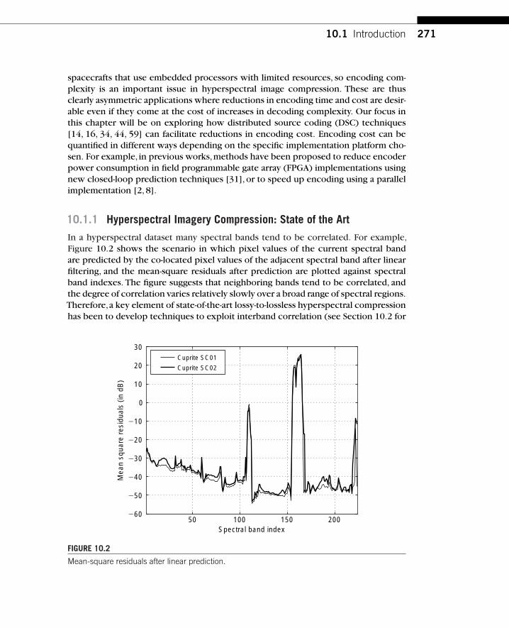
10.1 Introduction 271
spacecrafts that use embedded processors with limited resources, so encoding com-plexity is an important issue in hyperspectral image compression. These are thusclearly asymmetric applications where reductions in encoding time and cost are desir-able even if they come at the cost of increases in decoding complexity. Our focus inthis chapter will be on exploring how distributed source coding (DSC) techniques[14, 16, 34, 44, 59] can facilitate reductions in encoding cost. Encoding cost can bequantified in different ways depending on the specific implementation platform cho-sen. For example, in previous works,methods have been proposed to reduce encoderpower consumption in field programmable gate array (FPGA) implementations usingnew closed-loop prediction techniques [31], or to speed up encoding using a parallelimplementation [2, 8].
10.1.1 Hyperspectral Imagery Compression: State of the Art
In a hyperspectral dataset many spectral bands tend to be correlated. For example,Figure 10.2 shows the scenario in which pixel values of the current spectral bandare predicted by the co-located pixel values of the adjacent spectral band after linearfiltering, and the mean-square residuals after prediction are plotted against spectralband indexes. The figure suggests that neighboring bands tend to be correlated, andthe degree of correlation varies relatively slowly over a broad range of spectral regions.Therefore,a key element of state-of-the-art lossy-to-lossless hyperspectral compressionhas been to develop techniques to exploit interband correlation (see Section 10.2 for
50 100 150 200260
250
240
230
220
210
0
10
20
30
Spectral band index
Mea
n sq
uare
res
idua
ls (
in d
B)
Cuprite SC01
Cuprite SC02
FIGURE 10.2
Mean-square residuals after linear prediction.
272 CHAPTER 10 Distributed Compression of Hyperspectral Imagery
a more detailed discussion of the correlation characteristics that motivate the designof these algorithms):
■ In interband predictive approaches [31, 37, 48], a band is predicted usingpreviously encoded bands. The resulting prediction residuals can then beencoded using standard image coding techniques (e.g., transformation followedby quantization and entropy coding). Since,typically, the prediction residual hasa much lower energy than the original band, encoding it usually requires fewerbits than encoding the original band. Interband prediction approaches are anal-ogous to predictive video coding (e.g., the standard MPEG/H.26x compressionalgorithms), but a key difference is that motion estimation/compensation arenot necessary since co-located pixels in different spectral bands represent theresponses of the same ground object at different wavelengths. However, simplelinear prediction to align the values of co-located pixels of consecutive spectralbands has been found to be useful to improve the prediction gain [31].
■ 3D wavelet methods, including 3D SPIHT [15,21],3D SPECK [47], and 3D ICER[20, 22], provide alternatives to predictive coding. 3D wavelet methods exploitinterband correlation by performing filtering across spectral bands, with theexpectation that most of the signal energy will be concentrated in low-pass sub-bands (corresponding to low spatial and “cross-band” frequencies). Similar totypical 2D wavelet image coding,bit-plane coding is usually applied to the trans-form coefficients obtained from filtering. The resulting bits can be compressedwith entropy coding schemes such as zero-tree coding [41] or those based oncontext modeling [20].
As an example to illustrate 3D wavelet approaches, in 3D ICER [20,22], a modified3D Mallat decomposition is first applied to the image cube. Then mean values aresubtracted from the spatial planes of the spatially low-pass subbands to account forthe“systematic difference”in different image bands [22,23].1 Bit-plane coding is thenapplied to the transform coefficients, with each coefficient bit adaptively entropy-coded based on its estimated probability-of-zero statistics.The probability is estimatedby classifying the current bit to be encoded into one of several contexts according tothe significance status of the current coefficient and its spectral neighbors.A differentprobability model is associated with each context.
In addition, a lossy compression scheme using the Karhunen–Loève transform(KLT) and the discrete cosine transform (DCT) was proposed in [40]; several losslesscompression schemes have also been proposed for hyperspectral data, for example,those based on vector quantization [32, 39], and spatial, spectral, or hybrid prediction[38, 52, 58].
1 Note that mean subtraction in these 3D wavelet approaches is conceptually similar to using linearprediction to align the values of co-located pixels in order to account for the global offset in eachspatial image specific to hyperspectral data [22].
10.2 Hyperspectral Image Compression 273
10.1.2 Outline of This Chapter
Section 10.2 of this chapter discusses the general issues of hyperspectral data com-pression. Datasets and correlation characteristics of the commonly used NASA AVIRISdata will be discussed, followed by discussions on some potential problems in apply-ing interband prediction approaches and 3D wavelet approaches for hyperspectraldata. Motivated by these potential problems in conventional approaches, applica-tion of distributed coding principles for hyperspectral data compression will then bediscussed in Section 10.3,with a focus on the potential advantages and associated chal-lenges. Section 10.4 then summarizes several examples of DSC-based hyperspectralcompression algorithms. Section 10.5 concludes the chapter.
10.2 HYPERSPECTRAL IMAGE COMPRESSION
10.2.1 Dataset Characteristics
As illustrated in Figure 10.1, hyperspectral images are three-dimensional image cubes,with two spatial dimensions and one spectral dimension. A well-known example isthe NASA AVIRIS data, which consists of 224 spatial images [2, 24]. Each spatial lineof AVIRIS data has 614 pixels, and datasets with 512 spatial lines are commonly avail-able, leading to about 140M bytes of information. AVIRIS captures wavelengths from400 to 2500 nanometers, at a spectral resolution of about 10 nanometers. Spatial res-olution would depend on how high above the surface the scanning operations aretaking place. For example, at an altitude of 20 kilometers, AVIRIS has a spatial resolu-tion of 20 meters. In typical operations, spatial resolutions of 2 to 20 meters can beachieved [2, 45].
Pixel values of hyperspectral images along the spectral dimension provide impor-tant information regarding the extent of energy absorption and scattering at differentwavelengths of the captured objects. Figure 10.3 shows some examples of spectralcurves of hyperspectral image data. Different materials tend to exhibit different spec-tral responses [33]. Therefore, these spectral curves can be very useful for classifyingthe ground objects. It should be noted that, depending on the spatial resolution andhence the size of the ground resolution cell, the values of a pixel may include con-tributions from more than one material; that is, the hyperspectral data may representcomposite or mixed spectrum. The contribution from each material may depend onits area within a ground resolution cell [45].
Alternatively, spectral information of each pixel may also be represented as a spec-tral vector in the n-dimensional space, where n is the number of spectral bands, andthe response at each wavelength corresponding to the projection of the vector ontothe respective coordinate axis. This vector representation provides a useful mean forautomatic classification of the captured materials. For example, the similarity of twospectra can be measured by the angle between the corresponding spectral vectors,such as in the well-known spectral angle mapper (SAM) algorithm [13].

274 CHAPTER 10 Distributed Compression of Hyperspectral Imagery
0 50 100 150 200 2500
1000
2000
3000
4000
5000
6000
7000
8000
9000
10000
Spectral band index
Res
pons
es
FIGURE 10.3
Some examples of spectral responses in hyperspectral image dataset: NASA AVIRIS Cuprite.
From the perspective of lossy compression, it is therefore important to preservethe spectral characteristics of hyperspectral images, in addition to the average recon-struction fidelity (measured by peak signal-to-noise ratio (PSNR), for example) ofthe datasets. Lossy hyperspectral compression algorithms may be compared by theclassification performance of the reconstructed images, in addition to rate-distortionperformance [8, 47].
10.2.2 Intraband Redundancy and Cross-band Correlation
Hyperspectral applications may exploit the spatial and/or the spectral redundancyto achieve compression. The degree of spatial redundancy within each spectral bandwould obviously depend on the captured scene. Moreover, while the spatial imagesof a hyperspectral dataset represent captured data of the same scene and thereforethe spatial contents of most images would be similar, it is possible that some imagesmay have different spatial contents and hence different amounts of intraband redun-dancy,depending on the response characteristics of the ground objects. For example,Figure 10.4 shows several spatial images in a hyperspectral dataset. Notice that in thisexample the image data of the first spectral band is rather noisy.Therefore,correlationbetween pixels may not be high,impacting the performance of using intraband codingschemes to compress the data.
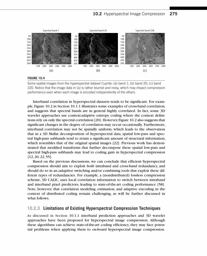
10.2 Hyperspectral Image Compression 275
Spectral band 1
100 200 300 400 500 600
50100150200250300350400450500
Spectral band 20
100 200 300 400 500 600
50100150200250300350400450500
Spectral band 220
100 200 300 400 500 600
50100150200250300350400450500
(a) (b) (c)
FIGURE 10.4
Some spatial images from the hyperspectral dataset Cuprite: (a) band 1; (b) band 20; (c) band220. Notice that the image data in (a) is rather blurred and noisy, which may impact compressionperformance even when each image is encoded independently of the others.
Interband correlation in hyperspectral datasets tends to be significant. For exam-ple, Figure 10.2 in Section 10.1.1 illustrates some examples of cross-band correlation,and suggests that spectral bands are in general highly correlated. In fact, some 3Dwavelet approaches use context-adaptive entropy coding where the context defini-tions rely on only the spectral correlation [20]. However,Figure 10.2 also suggests thatsignificant changes in the degree of correlation may occur occasionally. Furthermore,interband correlation may not be spatially uniform, which leads to the observationthat in a 3D Mallat decomposition of hyperspectral data, spatial low-pass and spec-tral high-pass subbands tend to retain a significant amount of structural information,which resembles that of the original spatial images [22]. Previous work has demon-strated that modified transforms that further decompose these spatial low-pass andspectral high-pass subbands may lead to coding gain in hyperspectral compression[12, 20, 22, 55].
Based on the previous discussions, we can conclude that efficient hyperspectralcompression should aim to exploit both intraband and cross-band redundancy, andshould do so in an adaptive switching and/or combining tools that exploit these dif-ferent types of redundancies. For example, a (nondistributed) lossless compressionscheme, 3D CALIC, uses local correlation information to switch between intrabandand interband pixel predictors, leading to state-of-the-art coding performance [58].Note, however, that correlation modeling, estimation, and adaptive encoding in thecontext of distributed coding remain challenging, as will be further discussed inwhat follows.
10.2.3 Limitations of Existing Hyperspectral Compression Techniques
As discussed in Section 10.1.1 interband prediction approaches and 3D waveletapproaches have been proposed for hyperspectral image compression. Althoughthese algorithms can achieve state-of-the-art coding efficiency, they may face poten-tial problems when applying them to on-board hyperspectral image compression.
276 CHAPTER 10 Distributed Compression of Hyperspectral Imagery
These potential problems serve as motivation to study new hyperspectral compressiontechniques based on DSC.
10.2.3.1 Interband Prediction ApproachesIn interband prediction approaches, previously encoded bands are used to predictthe current band and the resulting prediction residuals are then further compressed.Interband prediction approaches can in general achieve a high compression ratio withmoderate memory requirements. There are several drawbacks, however.
First, interband prediction methods need to generate exact copies of the decodedbands at the encoder, so encoders need to perform both encoding and decoding,2
and decoding complexity could be significant, for example, comparable to encodingcomplexity. Previous work has proposed to reduce the complexity of this decodingloop. For example, [31] has proposed using only full bit-planes to form the predic-tors at the encoder and decoder when using the Set Partitioning in Hierarchial Trees(SPIHT) algorithm [41] to compress the residue.This avoids bit-plane decoding at theencoder. However, since this approach does not utilize fractional bit-plane informa-tion in reconstruction, the predictors in general have worse qualities compared tothat of conventional interband prediction methods, leading to degradation in codingperformance.
Second, interband predictive methods are inherently serial, since each band isencoded based on a predictor obtained from previously encoded bands. Therefore,it is difficult to parallelize processing in order to improve the processing speed of aninterband predictive encoder to handle the high data rate generated by hyperspectralimaging instruments.
Third, it is difficult to achieve efficient rate scalability. This is because, whileinterband prediction approaches would stipulate identical predictors to be used inencoding and decoding, bit-rate scaling by on-the-fly truncation of the embedded bit-stream may, however, lead to different reconstructions at the decoder, depending onthe truncation points. Therefore, rate scaling could result in mismatches between thepredictors at the encoder and the decoder, leading to drift and degradation of thereconstruction quality.
10.2.3.2 3D Wavelet Approaches3D wavelet methods exploit interband correlation by performing filtering across spec-tral bands, which in general can lead to energy concentration in low-pass subbands.While 3D wavelet methods can achieve good compression efficiency with excellentscalability, a main disadvantage is that they lead to complex memory managementissues.A naive implementation would consist of loading several spectral bands in mem-ory so as to perform cross-band filtering, leading to expensive memory requirements.
2 The exception is the case when compression is lossless since the original images will be availablefor decoding and thus can be used for prediction.

10.3 DSC-based Hyperspectral Image Compression 277
More sophisticated approaches are possible (e.g., loading simultaneously only sub-bands corresponding to a given spatial frequency in various spectral bands),but theseapproaches have the drawback of requiring numerous iterations of memory access.
10.3 DSC-BASED HYPERSPECTRAL IMAGECOMPRESSION
Motivated by these potential drawbacks in existing hyperspectral image compressionalgorithms, several techniques based on DSC have been proposed recently [3,5,8,26,30, 46]. In this section, we first discuss the potential advantages of applying DSC forhyperspectral image compression, in terms of reduced encoding complexity, ease ofparallel encoding, and scalability. The challenges of applying DSC for hyperspectralcompression will also be discussed.
Figure 10.5 shows an example of how DSC may be applied to hyperspectralcompression. To decorrelate the input pixel data, the current spectral band Bi mayundergo some transformations. Outputs from the first stage (i.e., transform coeffi-cients,depicted as X in Figure 10.5) could then be compressed by DSC techniques toexploit interband correlation, using the corresponding data Y from the neighboringreconstructed band as side information in joint decoding. The key distinct feature ofDSC systems is that only the correlation information between X and Y (depicted asP(X, Y ) in Figure 10.5) is needed for encoding X . In particular, exact values of Ywould not be required. Therefore, DSC-based encoders could in principle operate in“open loop,” that is, without requiring that the encoders include decoding loops toreplicate data reconstructed at the decoders, as included in typical (lossy) interbandprediction approaches. Operating in open loop can lead to some system-level advan-tages,as will be discussed. If the correlation between X and Y is weak,encoders mightswitch to use intracoding to compress X .Also intraprediction might be applied beforeDSC encoding to exploit spatial redundancy. In practical applications, encoders mayneed to estimate the correlation information,which could be nontrivial in a distributedcomputing environment.
DSCEncoder
X XT
P (X, Y)
Bi BiDSCDecoder
ˆ ˆT 21
Y
FIGURE 10.5
An example of DSC-based hyperspectral image compression. “T ” and “T �1” denotetransformation and the inverse, respectively.

278 CHAPTER 10 Distributed Compression of Hyperspectral Imagery
10.3.1 Potential Advantages of DSC-based Hyperspectral Compression
10.3.1.1 Asymmetric Compression Framework with a Reduced ComplexityEncoder
Because of the limited available resources in satellites and spacecrafts,on-board encod-ing complexity is an important issue in hyperspectral compression. DSC may leadto an asymmetric framework where encoding complexity could be reduced at theexpense of some increases in decoding complexity at the ground station.This is possi-ble because, with DSC, encoding of the current spectral band would require only thecorrelation information. Therefore, computation and buffering storage for replicatingthe predictor would not be required in encoding, leading to complexity reduction.We remark that the complexity for“closing”the prediction loop could be nontrivial inlossy hyperspectral compression [31]. Note that a similar idea has also been appliedto scalable video coding to reduce the encoding complexity due to closing multipleprediction loops of different quality layers [53, 54].
In addition, the memory requirements of a DSC-based encoder tend to be mod-erate because correlation information may be estimated using data from consecutivespectral bands [6].This compares favorably to 3D wavelets methods,where pixel dataof multiple spectral bands is needed in cross-band filtering.
10.3.1.2 Parallel Encoding of DatasetsThe fact that DSC-based encoders can operate in open loop without being requiredto replicate the exact predictors may also lead to encoding algorithms that facilitateparallel implementation. For example, in encoding systems with multiple processors,compression of each entire spatial image may be assigned to each processor (seeFigure 10.6 in Section 10.4.2 for an example). As long as the cross-band correlationinformation between adjacent spectral bands is available,each processor can proceedindependently without further interaction during the course of encoding, leading tohighly parallel encoding systems. Moreover, information-theoretic results [44] sug-gest such DSC-based parallel encoding can in principle achieve competitive codingefficiency, for example, comparable to that of nondistributed schemes, where all thespectral bands reside at the same processor for centralized encoding.
10.3.1.3 ScalabilityDSC can also lead to hyperspectral compression systems that support more efficientrate scalability. Precisely, bit-rate scaling by on-the-fly truncation of an embedded bit-stream may result in several different possible predictor candidates available at thedecoder, each corresponding to the reconstruction at a truncation point. The actualpredictor present at the decoder would depend on the specific truncation pointchosen by the system. This uncertainty poses a challenge to interband predictionapproaches,where precise status of the available predictor at the decoder needs to bemaintained during encoding. In contrast, there is no need for a DSC encoder to knowabout the precise decoder predictor status. In particular,a DSC system may truncate anembedded bitstream,and as long as the side information matching (or exceeding) the

10.3 DSC-based Hyperspectral Image Compression 279
degree of correlation used in encoding can be reconstructed at the decoder,successfulSlepian–Wolf decoding can be achieved, leading to drift-free outputs [60]. In practice,the truncation points may be restricted by the block sizes used in Slepian–Wolf coding.Note that applying DSC to address multiple predictor candidates in video applicationshas been proposed in [7, 10] and to address scalable video streaming with feedbackin [42].
10.3.2 Challenges in Applying DSC for Hyperspectral Imaging
Information-theoretic results state that distributed encoding can be as efficient as jointencoding provided that different bitstreams are jointly decoded [14, 44, 59]. How-ever,achieving coding performance comparable to that of nondistributed approachesremains challenging for DSC hyperspectral image applications.This could be due to thedifficulties involved in modeling,estimating, and exploiting the correlation in hyper-spectral data, in a distributed setting (see Section 10.2.2 for a discussion of correlationcharacteristics).
First, while the coding efficiency of DSC depends strongly on the accuracy of thecorrelation models, real-world hyperspectral image data may exhibit nonstationaryand complex correlation structures. For example, local variations of spatial or spec-tral correlation may occur in hyperspectral datasets. Also, considerable dependencybetween individual (cross-band) correlation noise symbols may exist in hyperspectraldata [22].3 Therefore, i.i.d. noise models commonly used in DSC applications couldbe inadequate to capture the statistics of cross-band correlation noise in hyperspec-tral image compression. While utilizing more sophisticated models that capture thesecomplicated correlation structures may lead to better coding performance, it may bechallenging to design the coding algorithms and the correlation estimation techniquesfor such advanced models.
Second, correlation information in hyperspectral data may need to be estimatedunder complexity constraints, so that the potential advantage of applying DSC toreduce encoder power consumption could be realized. For example, some relativelycomputationally intensive estimation techniques (e.g., the expectation-maximization(EM) algorithm [29]) may not be suitable for on-board correlation estimation in hyper-spectral applications. Also, in distributed encoding scenarios, only a small number ofsamples may be exchanged in order to reduce the communication overheads,but usinglow sampling rates may fail to capture the local changes in correlation. These com-plexity and rate constraints therefore make on-board correlation estimation a difficulttask [9]. While some DSC applications may employ feedback channels to acquire thecorrelation information from the decoder [1, 18], in hyperspectral applications, thisinformation may need to be estimated on-board during encoding, as feedback fromthe ground station may incur considerable delay.
3 Previous work has reported that spectral high-pass coefficients can exhibit spatial structureresembling that of the original spatial images [22].

280 CHAPTER 10 Distributed Compression of Hyperspectral Imagery
Third,to efficiently exploit the correlation in hyperspectral images the compressionalgorithms may need to be highly adaptive to the local variations of spatial or spectralcorrelation (such as in the case of 3D CALIC as briefly discussed in Section 10.2.2). Onthe other hand, achieving such a level of adaptivity using DSC could be challenging.For example,existing Slepian–Wolf coders usually employ capacity approaching error-correcting codes to perform data compression, and these codes tend to require largeblock sizes, for example,of the order of 105 [27,60];otherwise significant performancedegradation may result. However, large encoding block sizes may not be able to exploitthe changes in correlation in small blocks of hyperspectral data. Recent work hasproposed addressing distributed compression based on arithmetic coding,which mayachieve good coding performance with much smaller block sizes, for example, of theorder of 103 [17],and this code could be more suitable for hyperspectral applications.
In addition, since one of the main applications of hyperspectral data is to identifythe captured objects, it is important for DSC-based lossy compression algorithms topreserve the spectral characteristics (see Section 10.2.1).
10.4 EXAMPLE DESIGNSIn this section we discuss several DSC-based hyperspectral image compression algo-rithms proposed in the literature. Specifically, we discuss in Section 10.4.1 the twolossless compression algorithms proposed by Magli et al. [30], in Section 10.4.2 thewavelet-based lossy-to-lossless algorithm proposed by Tang et al. [46],Cheung et al. [8],and Cheung and Ortega [5], and in Section 10.4.3 the multispectral compressionalgorithm proposed by Li [26]. Both the first lossless algorithm in Section 10.4.1and the wavelet-based algorithm in Section 10.4.2 exploit intra- and interband redun-dancy. However, the specific mechanisms are rather different: the first algorithm inSection 10.4.1 applies intraprediction to pixel data, and then the prediction residuewould be further compressed by DSC exploiting cross-band correlation. The algorithmin Section 10.4.2, however, uses wavelet transform and bit-plane extraction similar toSPIHT to generate different types of source bits, each with different marginal andjoint statistics (w.r.t. side information), and based on these statistics the bits are thenadaptively compressed by either intra (zero-tree coding) or inter (DSC) approaches.In contrast to these algorithms that use capacity-approaching large-block-size error-correcting codes to compress the binary bits, the second algorithm in Section 10.4.1uses a simple multilevel coset code to compress individual symbols so that better adap-tation to local correlation statistics can be achieved. The algorithm in Section 10.4.3uses different constraints to iteratively refine coarsely encoded spectral band images.
10.4.1 DSC Techniques for Lossless Compression of HyperspectralImages
Lossless compression of hyperspectral imagery based on DSC has been proposedby Magli et al. [30]. In this work, DSC is used to exploit the correlation between
10.4 Example Designs 281
different spectral bands. This is combined with other techniques, such as the pre-diction stage of 2D CALIC [57], to exploit intraband correlation. The main purposeis to shift complexity, in particular computational operations, from the encoder tothe decoder, by relying on the decoder to exploit spatial correlation, similar in spiritto low-complexity video encoding [1,16,35,36]. Specifically, the work proposed twoalgorithms for data compression,one based on powerful binary error-correcting codesand the other based on simpler multilevel coset codes (to be discussed in more detailin the subsequent sections).
10.4.1.1 Lossless Hyperspectral Compression Based on ErrorCorrecting Codes
The first proposed algorithm is based on capacity approaching binary error-correctingcodes such as Slepian–Wolf (SW) codes.
The algorithm operates on pixel data when compressing the current spectralband and exploits intraband redundancy by applying to each pixel a 2D CALIC pre-dictor formed by spatially adjacent pixels. Denote the spatial prediction error array byEX , and the spatial prediction error array of the previous band after linear filtering byE�Y. EX are losslessly compressed based on DSC techniques using E�Y as side informa-tion. Specifically, EX are decomposed into a raw bit-plane representation. Denote theextracted raw bit-planes by E(b)
Xi, where 0� i �NEX is the significance level of the bit-
plane and NEX is the number of extracted bit-planes. Denote also the corresponding
bit-planes in E�Y by E�(b)
Yi. Binary sources E(b)
Xiare compressed by a LDPC-based SW coder,
using E�(b)
Yiin joint decoding at the decoder. The SW encoding rate of each bit-plane
is derived from the conditional entropy of the input bits given the side informationbits, H(E(b)
Xi|E�
(b)Yi
), assuming the bits are i.i.d. binary sources and the correlation canbe modeled by a binary channel. Depending on the conditional entropy and the effi-ciency of the SW coder,some bit-planes would instead be compressed by an arithmeticcoder.
The encoding rate or the conditional entropy H(E(b)Xi|E�
(b)Yi
) would depend on the
correlation between bits E(b)Xi
and E�(b)
Yi. In [30],this correlation information is assumed
to be known, and there is no discussion related to efficient estimation of this infor-mation. It should be noted that this correlation estimation problem could be non-trivial and remains to be a challenging issue in practical application of DSC [18]. Astraightforward approach that exchanges all the bit data for direct comparison wouldinevitably incur significant communication overhead and may upset the complexitysaving due to DSC techniques (see more discussion in [11]).
The proposed algorithm was compared with several 2D and 3D lossless compres-sion schemes using NASA AVIRIS datasets, and experimental results reported in [30]suggest the proposed algorithm can outperform 2D coding techniques (specifically,JPEG-LS) by about 1 bit per pixel (bpp) on average, while there is still a performancegap of about 1 bpp compared to 3D CALIC. According to [30], this performancegap is partly due to the sophisticated context modeling techniques in 3D CALICthat capture local spatial and spectral correlation (see Section 10.2.2 for correlation
282 CHAPTER 10 Distributed Compression of Hyperspectral Imagery
characteristics),and partly caused by the inefficiency in assuming a binary correlationmodel that ignores the correlation between bit-planes of different significances [56].
10.4.1.2 Lossless Hyperspectral Compression Based on MultilevelCoset Codes
In [30] another lossless hyperspectral compression algorithm based on simplermultilevel coset codes was proposed.
The algorithm adopts a block-based approach,where the spatial images are split intononoverlapping small blocks, and correlation estimation is performed on each blockindependently to estimate the coding rate based on direct comparisons of a subsetof pixels of the corresponding block in the adjacent spectral band. Using a block-based approach allows fine adaption in the estimation of interband dependencies,which tends to be nonstationary. This, however, complicates application of capacityapproaching error-correcting codes in SW coding, which would in general requireblock lengths of several thousands of symbols.
To address this issue,Magli et al. [30] proposed using simple multilevel coset codesthat encode each symbol (corresponding to a pixel in this case), independently usingas side information the corresponding symbol in the neighboring spectral band. Specif-ically, for each pixel x(i, j) in the current spectral band, Magli et al. [30] propose acorrelation model4
x(i, j)�P( y(i, j))�n(i, j), (10.1)
where n(i, j) is the correlation noise, and y(i, j) is the value of the correspondingpixel in neighboring spectral band. P is a prediction model to estimate x(i, j) fromy(i, j). Depending on the statistics of n(i, j), only the k least significant bits (LSB) ofx(i, j) would be communicated to the decoder, and the decoder would use the sideinformation y(i, j) and P to infer the discarded most significant bits (MSB) of x(i, j).With accurate estimation of n(i, j), the value of k that leads to exact recovery of x(i, j)can be derived. In [30], k is determined for each block based on the maximum valueof n(i, j) over the block,estimated based on exchanging some subsets of pixels x(i, j)and y(i, j).
Experimental results reported in [30] suggest that, in this particular applicationusing NASA AVIRIS datasets,the proposed block-based adaptive coding algorithm usingsimple multilevel codes can achieve similar performance to its counterpart based onpowerful error-correcting codes, that is, on average outperforming JPEG-LS by about1 bpp,while compared to 3D CALIC there is still a 1-bpp performance gap. Regardingexecution time, for simulations running on a workstation, where correlation estima-tion complexity has been taken into account but the spectral bands were available inthe same location, [30] reported the proposed algorithm is about 10 times faster than3D CALIC.
4 Note that here cross-band correlation is exploited between pixels data rather than the intrapredictionresidues as in the first algorithm.

10.4 Example Designs 283
10.4.2 Wavelet-based Slepian–Wolf Coding for Lossy-to-losslessCompression of Hyperspectral Images
Wavelet-based algorithms for lossy-to-lossless compression of hyperspectral imageshave been proposed [5, 8, 46]. The proposed algorithm combines set partitioning ofwavelet coefficients such as that introduced in the popular SPIHT algorithm [41] withDSC techniques,so that sign bits would be compressed by SW coding,while magnitudebits would be encoded using adaptive combinations of DSC and zero-tree coding. UsingDSC tools allows the encoder to operate in open loop without requiring access todecoded versions of neighboring spectral bands, and this facilitates parallel encodingof spectral bands in multiprocessor architectures. The memory requirement of theproposed algorithm is modest and similar to that of interband prediction approaches.Note that wavelet-based DSC algorithms have also been subsequently proposed fordistributed video and sensors applications [19, 50].
10.4.2.1 System OverviewFigure 10.6 shows an overview of the proposed encoding system in [5, 8, 46]. Theproposed encoder consists of multiple processors, and each processor compressesone entire spatial image at a time, using the algorithm to be discussed in detail in thenext section. With a DSC approach, encoding needs only the correlation informationin order to exploit interband redundancy. In particular, as long as the correlationinformation is available, each encoding thread compressing one spatial image wouldbe able to proceed in parallel, and parallel encoding of a hyperspectral dataset can beachieved.
Spectralband
Processor
Processor
Processor
Processor
Y
XP (X, Y )
Parallelencoding
Compressed data
FIGURE 10.6
Parallel encoding system based on DSC as proposed in [5, 8, 46]. Each processor compressesone spatial image at a time.
284 CHAPTER 10 Distributed Compression of Hyperspectral Imagery
One key issue for the proposed system is how to estimate the correlation informa-tion efficiently during encoding. However,correlation estimation may be nontrivial inthis setting, for the following reasons:
■ The spatial images of different spectral bands reside in different processors, andthe communication bandwidth between the processors could be limited.
■ Data exchanges between the processors may impact parallel encoding, as theprocessors may have to remain idle to wait for the data.
To address these constraints, sampling-based techniques have been proposed to per-form correlation estimation, with small amounts of interprocessor communicationoverhead and minimal dependencies between different encoding threads [8].
10.4.2.2 Encoding AlgorithmFigure 10.7 depicts the encoding algorithm.To compress the current spectral band Bi ,the proposed algorithm applies the wavelet transform and then bit-plane extractionsimilar to SPIHT to iteratively extract sign, refinement, significance information or,alternatively,using raw bit-planes from the wavelet coefficients [41,49].The extractedbit-planes are then compressed by SW coding to exploit interband correlation, orzero-tree coding to exploit intraband redundancy,depending on the correlation charac-teristics and the coefficients distributions [5]. Bit-planes are progressively transmittedto the decoder starting from the most significant bit (MSB), and the number of bit-planes communicated would depend on the data rate or the quality requirementsof the particular application. Lossless compression can be achieved by using integerwavelets and transmitting all the bit-planes.
In SW coding of bit-planes, the proposed algorithm uses as side information thecorresponding bit-planes of the adjacent spectral band available at another processor.For example, the refinement bits of the current spectral band would be compressedusing the same magnitude bits extracted from the adjacent spectral band (after linearprediction) as side information.The bits are assumed to be i.i.d. sources,and the corre-lation w.r.t. the side information bits is modeled as a binary channel parameterized bythe crossover probability between the bits data,5 which needs to be estimated duringencoding to determine the SW encoding rate.
10.4.2.3 Correlation EstimationA straightforward approach to estimate the crossover probability could be to explic-itly generate and extract the side information bits from the adjacent spectral band atanother processor, and exchange and compare the source and side information bits,to determine the crossover probability. However, information exchange in the middle
5 Crossover probability is basically the probability that input bits are different from the correspondingbits in the side information. Small crossover probability therefore implies high correlation among thebits data.
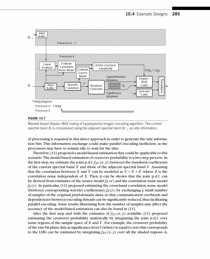
10.4 Example Designs 285
WaveletTransform
Significancebit-planes
Sign/refinementbit-planes
mul
tiple
Bit-planesExtraction
InputBuffer
InputBuffer
Processor k � 1
Pr[bx��by]
X
Slepian–Wolf
Coder
Zero-treeCoder
LinearPredictor
Derive crossoveranalytically
EstimateCorrelation
Noise Model EstimateSourceModel
Processor k
Bi�1
Bi bx
Processor k � 1
Timing Diagram:
Processor k
FIGURE 10.7
Wavelet-based Slepian–Wolf coding of hyperspectral images: encoding algorithm. The currentspectral band Bi is compressed using the adjacent spectral band Bi�1 as side information.
of processing is required in this direct approach in order to generate the side informa-tion bits. This information exchange could make parallel encoding inefficient, as theprocessors may have to remain idle to wait for the data.
Therefore,[11] proposed a model-based estimation that could be applicable to thisscenario.The model-based estimation of crossover probability is a two-step process. Inthe first step,we estimate the joint p.d.f. fXY (x, y),between the transform coefficientsof the current spectral band X and those of the adjacent spectral band Y . Assumingthat the correlation between X and Y can be modeled as Y �X �Z , where Z is thecorrelation noise independent of X . Then, it can be shown that the joint p.d.f. canbe derived from estimates of the source model fX (x) and the correlation noise modelfZ (z). In particular, [11] proposed estimating the cross-band correlation noise model(between corresponding wavelet coefficients), fZ (z), by exchanging a small numberof samples of the original pixel-domain data, so that communication overheads anddependencies between encoding threads can be significantly reduced,thus facilitatingparallel encoding. Some results illustrating how the number of samples may affect theaccuracy of the model-based estimation can also be found in [11].
After the first step and with the estimates of fXY (x, y) available, [11] proposedestimating the crossover probability analytically by integrating the joint p.d.f. oversome regions of the sample space of X and Y . For example, the crossover probabilityof the raw bit-plane data at significance level l (when l is equal to zero this correspondsto the LSB) can be estimated by integrating fXY (x, y) over all the shaded regions Ai

286 CHAPTER 10 Distributed Compression of Hyperspectral Imagery
|Y |
|X |0
3 � 2l
3 � 2l
2 � 2l
2 � 2l
2l
2l
…
…
A0
A1
A3
A2
Ai
A4
A5
FIGURE 10.8
Model-based approach for crossover probability estimation. Ai are the events that lead tooccurrence of raw bit-plane crossovers between X and Y at significance level l.
as shown in Figure 10.8. In practice, only a few regions that lead to nonzero integralsneed to be considered.The crossover estimates for sign and refinement bit-planes canbe derived following the same procedure, as discussed in [11].
10.4.2.4 Adaptive Combination of DSC and Zero-tree CodingTo improve the coding performance, [5] proposed an algorithm to adaptively encodethe magnitude bits using DSC or zero-tree coding. Specifically, magnitude bits may beextracted as raw bit-planes and compressed using SW coding.Alternatively,magnitudebits may also be partitioned into refinement bit-planes and significance informationbit-planes, and compressed using SW coding and zero-tree coding, respectively. Todetermine the switching strategy between the two schemes, modeling techniqueswere proposed in [5] to estimate the relative coding efficiencies of the SW codingand zero-tree coding approaches, using the marginal distribution fX (x) and the jointp.d.f. fXY (x, y). Estimates of the number of coded bits using DSC and zero-tree codingare derived from these p.d.f. at each significance level, and also separately for eachwavelet subband.
Figure 10.9 shows some modeling results of two wavelet subbands,which illustratehow the number of coded bits (estimated by modeling) changes with the significancelevels.The modeling results suggest that,at high significance levels,it tends to be moreefficient to partition the magnitude bits into refinement bit-planes and significanceinformation bit-planes, and compress them using SW coding and zero-tree coding,respectively (labeled “DSC � ZTC” in Figure 10.9). On the other hand, in the middlesignificance levels, it may be possible to achieve better coding performance byswitching to another scheme that extracts the magnitude bits as raw bit-planes andencodes them using SW coding only (labeled “DSC” in Figure 10.9). The figuresshow that these switchings should occur at certain significance levels in order toobtain the optimal compression results. Different wavelet subbands would havedifferent switching levels, and the optimal switching levels can be determined usingthe modeling techniques in [5].

10.4 Example Designs 287
Num
ber
of c
oded
bits
(es
timat
ed)
Num
ber
of c
oded
bits
(es
timat
ed)
High-level subbandband 4
DSC
DSC � ZTC
Switching threshold
300
250
200
150
100
50
00 2 4 6 8 10 12 14 16
Switching threshold
Low-level subbandband 14
DSC
DSC � ZTC
70000
60000
50000
40000
30000
20000
10000
00 2 4 6 8 10 12 14 16
(a) The 4th subband (b) The 14th subband
Significance level Significance level
FIGURE 10.9
The amounts of coded bits (estimated by modeling) vs. the significance levels of two waveletsubbands.
Cuprite Radiance (Scene SC01, Band 131–138)
65
70
75
80
85
90
95
0.1 1 10
Bitrate (bits/pixel/band)
MP
SN
R (
dB)
DSC (Adaptive)
DSC (Nonadaptive)
Latest 3D ICER (Apr 06)
FY04 3D ICER
SPIHT
FIGURE 10.10
Coding performance of the DSC algorithm proposed in [5, 8, 46]: NASA AVIRIS Cuprite datasets.Reconstruction qualities are measured by MPSNR, the average PSNR of multiple spectral bands.

288 CHAPTER 10 Distributed Compression of Hyperspectral Imagery
10.4.2.5 Coding PerformanceFigure 10.10 shows the performance of the wavelet-based DSC algorithm along withseveral 3D wavelet algorithms (3D ICER) developed by NASA-JPL [20] for encodingNASA AVIRIS datasets. As shown in the figure, the DSC algorithm with adaptive cod-ing is comparable to a simple 3D wavelet system (FY04 3D ICER) in terms of codingefficiency.The simple 3D wavelet system uses the standard dyadic wavelet decomposi-tion and a context-adaptive entropy coding scheme to compress transform coefficientsbits. However,there still is a performance gap when comparing the DSC algorithm to amore recent and sophisticated version of 3D wavelet (latest 3D ICER).The more recent3D wavelet developed in NASA-JPL exploits the spatial correlation that still exists inthe correlation noise [20]. The results indicate further improvement may be possiblein the DSC algorithm, which currently uses a simple i.i.d. model for correlation noiseand ignores the dependency between correlation noise symbols. Figure 10.10 alsoshows that when compared with 2D SPIHT the DSC algorithm can achieve 8 dB gainsat some bit rates.
10.4.3 Distributed Compression of Multispectral Images Using a SetTheoretic Approach
DSC-based lossy compression of multispectral images was proposed in [26].The mainpurpose of the proposed work is to compress image data corresponding to differ-ent spectral channels of the same scene, using several spatially separated encoders.A set-theoretic framework for distributed compression was proposed. Specifically, thecross-band correlation and observation constraint are assumed to be characterizedby convex sets. Following from the convex set assumptions, joint decoding of multi-spectral images can be implemented via iterative projection-onto-convex-set (POCS)operations at the centralized decoder, and the convexity of constraint sets guaranteesthe convergence of the decoding algorithm.
In one of the scenarios considered in [26], spatial images X1, X2, . . . , XK are com-pressed using an asymmetric protocol, where X1 shall be intracoded at a relativelyhigh quality, and the decoded version of X1 would serve as side information fordecoding the DSC compressed images X2, . . . , XK . Li [26] proposed that the spa-tial images Xk, 2�k�K could be wavelet transformed and coarsely quantized. Thereconstruction of Xk can be iteratively refined, at the decoder, using the followingconstraints:
■ Cross-band correlation structure: co-located wavelet coefficients of X1 and Xk
are assumed to be less than some threshold.■ Observation constraint of image source: each of the wavelet coefficients of Xk
can only assume values in its own quantization bin.
Li [26] argues that these constraint sets are convex, and the process of refining Xk
can be cast as the problem of identifying a point at the intersection of these convex sets,which can be implemented by alternatively projecting onto the defined convex sets.

References 289
Preliminary results in [26], however, indicate that the proposed algorithm is 2 dBless efficient compared to JPEG2000 intraband coding when applying it to RGB colorimages.This may be partly due to the assumed cross-band correlation model incapableof exploiting local correlation variations between co-located wavelet coefficients.
10.5 CONCLUSIONSIn this chapter we have discussed distributed compression of hyperspectral images.Motivated by the potential problems in conventional hyperspectral compressionapproaches, applications of DSC for hyperspectral data compression have been pro-posed in the literature. Potentially, DSC can lead to hyperspectral systems withreduced complexity encoders that facilitate parallel encoding and scalability, suitablefor the specific operating conditions in hyperspectral data acquisition. Several exam-ples of DSC-based hyperspectral compression algorithms proposed in the literaturewere summarized. While some of these DSC systems have demonstrated compet-itive rate-distortion efficiency, there are still performance gaps w.r.t. sophisticatednondistributed approaches. Future research direction could be to investigate improvedalgorithms with better adaptation to local variations in correlation.
REFERENCES[1] A. Aaron, R. Zhang, and B. Girod. Wyner–Ziv coding of motion video. In Proc.Asilomar Conf.
Signals, Systems, and Computers, November 2002.
[2] N. Aranki. Parallel implementations of the discrete wavelet transform and hyperspec-tral data compression on reconfigurable platforms: Approach, methodology and practicalconsiderations. Ph.D. thesis, University of Southern California, August 2007.
[3] M. Barni, D. Papini, A. Abrardo, and E. Magli. Distributed source coding of hyperspectralimages. In Proc. Int’l Symp.Geoscience and Remote Sensing (IGARSS), 2005.
[4] C. H. Chen. Information Processing for Remote Sensing.World Scientific Publishing Company,2000.
[5] N.-M. Cheung andA. Ortega.An efficient and highly parallel hyperspectral imagery compressionscheme based on distributed source coding. In Proc. Asilomar Conf. Signals, Systems, andComputers, 2006.
[6] N.-M. Cheung andA. Ortega.A model-based approach to correlation estimation in wavelet-baseddistributed source coding with application to hyperspectral imagery. In Proc. Int’l Conf. ImageProcessing (ICIP), 2006.
[7] N.-M. Cheung andA. Ortega. Distributed source coding application to low-delay free viewpointswitching in multiview video compression. In Proc. Picture Coding Symposium (PCS), 2007.
[8] N.-M. Cheung, C. Tang, A. Ortega, and C. S. Raghavendra. Efficient wavelet-based predictiveSlepian-Wolf coding for hyperspectral imagery. EURASIP Journal on Signal Processing—Special Issue on Distributed Source Coding, 86(11):3180–3195, November 2006.
[9] N.-M. Cheung, H. Wang, and A. Ortega. Correlation estimation for distributed source codingunder information exchange constraints. In Proc. Int’l Conf. Image Processing (ICIP), 2005.

290 CHAPTER 10 Distributed Compression of Hyperspectral Imagery
[10] N.-M. Cheung, H. Wang, and A. Ortega. Video compression with flexible playback order basedon distributed source coding. In Proc.Visual Communications and Image Processing (VCIP),2006.
[11] N.-M. Cheung, H. Wang, and A. Ortega. Sampling-based correlation estimation for distributedsource coding under rate and complexity constraints. IEEE Trans. Image Processing, 2008.
[12] E. Christophe and W. A. Pearlman. Three-dimensional SPIHT coding of volume images withrandom access and resolution scalability. EURASIP Journal on Image and Video Processing.Submitted, 2008.
[13] R. N. Clark, G. Swayze, J. Boardman, and F. Kruse. Comparison of three methods for materialsidentification and mapping with imaging spectroscopy. In Proc. JPL AVIRIS Airborne Geo-science Workshop, 1993.
[14] T. M. Cover and J. A. Thomas. Elements of Information Theory. NY: Wiley, 1991.
[15] P. L. Dragotti, G. Poggi, and A.R.P. Ragozini. Compression of multispectral images by three-dimensional SPIHT algorithm. IEEE Trans. Geoscience and Remote Sensing, 38(1):416–428,January 2000.
[16] B. Girod, A. Aaron, S. Rane, and D. Rebollo-Monedero. Distributed video coding. Proceedingsof the IEEE, Special Issue on Advances in Video Coding and Delivery, 93(1):71–83, January2005.
[17] M. Grangetto, E. Magli, and G. Olmo. Distributed arithmetic coding. IEEE CommunicationsLetters, 11(11):883–885, November 2007.
[18] C. Guillemot, F. Pereira, L. Torres, T. Ebrahimi, R. Leonardi, and J. Ostermann. Distributedmonoview and multiview video coding. IEEE Signal Processing Magazine, 24(5):67–76,September 2007.
[19] X. Guo, Y. Lu, F. Wu, W. Gao, and S. Li. Wyner–Ziv video coding based on set partitioning inhierarchical tree. In Proc. Int’l Conf. Image Processing (ICIP), 2006.
[20] A. Kiely, M. Klimesh, H. Xie, and N. Aranki. ICER-3D: A progressive wavelet-based com-pressor for hyperspectral images. Technical report, NASA-JPL IPN Progress Report, 2006.http://ipnpr.jpl.nasa.gov/progress_report/42-164/164A.pdf.
[21] B. Kim and W. A. Pearlman. An embedded wavelet video coder using three-dimensional setpartitioning in hierarchical tree. In Proc.Data Compression Conference (DCC), 1997.
[22] M. Klimesh, A. Kiely, H. Xie, and N. Aranki. Spectral ringing artifacts in hyperspectral imagedata compression. Technical report, NASA-JPL IPN Progress Report, 2005. http://ipnpr.jpl.nasa.gov/progress_report/42-160/160C.pdf.
[23] M. Klimesh, A. Kiely, H. Xie, and N. Aranki. Spectral Ringing Artifacts in HyperspectralImage Data Compression. In Giovanni Motta, Francesco Rizzo, and James A. Storer, editors,Hyperspectral Data Compression. Springer, 2006.
[24] NASA Jet Propulsion Laboratory. AVIRIS homepage. http://aviris.jpl.nasa.gov/, October 2007.
[25] D. Landgrebe. Hyperspectral image data analysis. IEEE Signal Processing Magazine, 19(1):17–28, January 2002.
[26] X. Li. Distributed coding of multispectral images: A set theoretic approach. In Proc. Int’l Conf.Image Processing (ICIP), 2004.
[27] A. D. Liveris, Z. Xiong, and C. N. Georghiades. Compression of binary sources with side infor-mation at the decoder using LDPC codes. IEEE Communications Letters, 6(10):440–442,October 2002.
[28] R. Lockwood, T. Cooley, R. Nadile, J. Gardner, P. Armstrong, A. Payton, T. Davis, S. Straight,T. Chrien,E. Gussin,and D. Makowski. Advanced responsive tactically-effective military imagingspectrometer (ARTEMIS) design. In Proc.Int’l Symp.Geoscience and Remote Sensing (IGARSS),2006.
References 291
[29] D.J.C. MacKay. InformationTheory, Inference, and LearningAlgorithms. Cambridge UniversityPress, 2003.
[30] E. Magli, M. Barni, A. Abrardo, and M. Grangetto. Distributed source coding techniques forlossless compression of hyperspectral images. EURASIP Journal on Applied Signal Processing,2007. Article ID 45493. 13 pages.
[31] A. C. Miguel, A. R. Askew, A. Chang, S. Hauck, and R. E. Ladner. Reduced complexity wavelet-based predictive coding of hyperspectral images for FPGA implementation. In Proc. DataCompression Conference (DCC), 2004.
[32] G. Motta, F. Rizzo, and J. A. Storer. Compression of hyperspectral imagery. In Proc. DataCompression Conference (DCC), 2003.
[33] California Institute of Technology. ASTER spectral library. http://speclib.jpl.nasa.gov/, 2000.
[34] S. Pradhan and K. Ramchandran. Distributed source coding using syndromes (DISCUS):Designand construction. In Proc.Data Compression Conference (DCC), 1999.
[35] R. Puri, A. Majumdar, and K. Ramchandran. PRISM: A video coding paradigm with motionestimation at the decoder. IEEE Trans. Image Processing, 16(10):2436–2448, October 2007.
[36] R. Puri and K. Ramchandran. PRISM: A new robust video coding architecture based ondistributed compression principles. In Proc. Allerton Conf. Communications, Control, andComputing, October 2002.
[37] A. K. Rao and S. Bhargava. Multispectral data compression using bidirectional interbandprediction. IEEE Trans.Geoscience and Remote Sensing, 34(2):385–397, March 1996.
[38] R. E. Roger and M. C. Cavenor. Lossless compression of AVIRIS images. IEEE Trans. ImageProcessing, 5(5):713–719, May 1996.
[39] M. J. Ryan and J. F. Arnold. The lossless compression of AVIRIS images by vector quantization.IEEE Trans.Geoscience and Remote Sensing, 35(3):546–550, May 1997.
[40] J. A. Saghri, A. G. Tescher, and J. T. Reagan. Practical transform coding of multispectralimagery. IEEE Signal Processing Magazine, 12(1):32–43, January 1995.
[41] A. Said and W. A. Pearlman. A new, fast, and efficient image codec using set partitioningin hierarchical trees. IEEE Trans. Circuits and Systems for Video Technology, 6(3):243–250,June 1996.
[42] A. Sehgal, A. Jagmohan, and N. Ahuja. Scalable video coding using Wyner–Ziv codes. In Proc.Picture Coding Symposium (PCS), December 2004.
[43] V. Shettigara and G. Fowler. Target re-acquisition capability of hyperspectral technology. InProc. Land Warfare Conference, pages 257–265, October 2005.
[44] D. Slepian and J. K. Wolf. Noiseless coding of correlated information sources. IEEE Trans.Information Theory, 19(4):471–480, July 1973.
[45] R. B. Smith. Introduction to hyperspectral imaging. Technical report, MicroImages, 2001.http://www.microimages.com/getstart/pdf/hyprspec.pdf.
[46] C. Tang, N.-M. Cheung, A. Ortega, and C. S. Raghavendra. Efficient inter-band prediction andwavelet based compression for hyperspectral imagery:A distributed source coding approach.In Proc.Data Compression Conference (DCC), 2005.
[47] X. Tang and W. A. Pearlman. Lossy-to-lossless block-based compression of hyperspectralvolumetric data. In Proc. Int’l Conf. Image Processing (ICIP), 2004.
[48] S. R. Tate. Band ordering in lossless compression of multispectral images. In Proc. DataCompression Conference (DCC), pages 311–320, 1994.
[49] D. Taubman and M. Marcellin. JPEG2000: Image Compression Fundamentals, Standards andPractice. Kluwer, 2002.
[50] V. Thirumalai, I. Tosic, and P. Frossard. Distributed coding of multiresolution omnidirectionalimages. In Proc. Int’l Conf. Image Processing (ICIP), 2007.

292 CHAPTER 10 Distributed Compression of Hyperspectral Imagery
[51] H. van der Werff. Knowledge based remote sensing of complex objects: recognition of spectraland spatial patterns resulting from natural hydrocarbon seepages. Ph.D. thesis, UniversiteitUtrecht, Utrecht, Netherlands, 2006.
[52] H.Wang,S. D. Babacan,and K. Sayood. Lossless hyperspectral image compression using context-based conditional averages. In Proc.Data Compression Conference (DCC), 2005.
[53] H. Wang, N.-M. Cheung, and A. Ortega. WZS: Wyner–Ziv scalable predictive video coding. InProc. Picture Coding Symposium (PCS), December 2004.
[54] H. Wang, N.-M. Cheung, and A. Ortega. A framework for adaptive scalable video codingusing Wyner–Ziv techniques. EURASIP Journal on Applied Signal Processing, 2006. ArticleID 60971. 18 pages.
[55] Y. Wang, J. T. Rucker, and J. E. Fowler. Three-dimensional tarp coding for the compres-sion of hyperspectral images. IEEE Geoscience and Remote Sensing Letters, 1(2):136–140,April 2004.
[56] R. P. Westerlaken, S. Borchert, R. K. Gunnewiek, and R. L. Lagendijk. Analyzing symbol and bitplane-based LDPC in distributed video coding. In Proc. Int’l Conf. Image Processing (ICIP),2007.
[57] X.Wu and N. Memon. Context-based,adaptive, lossless image coding. IEEE Trans.Communica-tions, 45(4):437–444, April 1997.
[58] X. Wu and N. Memon. Context-based lossless interband compression—extending CALIC. IEEETrans. Image Processing, 9(6):994–1001, June 2000.
[59] A. D. Wyner and J. Ziv. The rate-distortion function for source coding with side information atthe decoder. IEEE Trans. Information Theory, 22(1):1–10, January 1976.
[60] Z. Xiong, A. Liveris, and S. Cheng. Distributed source coding for sensor networks. IEEESignal Processing Magazine, 21(5):80–94, September 2004.

CHAPTER
11Securing Biometric Data
Anthony VetroMitsubishi Electric Research Laboratories, Cambridge, MA
Stark C. DraperDepartment of Electrical and Computer Engineering, University of Wisconsin,
Madison, WI
Shantanu Rane and Jonathan S. YedidaMitsubishi Electric Research Laboratories, Cambridge, MA
C H A P T E R C O N T E N T SIntroduction . . . . . . . . . . . . . . . . . . . . . . . . . . . . . . . . . . . . . . . . . . . . . . . . . . . . . . . . . . . . . . . . . . . . . . . . . . . . . . 294
Motivation and Objectives. . . . . . . . . . . . . . . . . . . . . . . . . . . . . . . . . . . . . . . . . . . . . . . . . . . . . . . . . . 294Architectures and System Security. . . . . . . . . . . . . . . . . . . . . . . . . . . . . . . . . . . . . . . . . . . . . . . . . 295Chapter Organization . . . . . . . . . . . . . . . . . . . . . . . . . . . . . . . . . . . . . . . . . . . . . . . . . . . . . . . . . . . . . . . 296
Related Work. . . . . . . . . . . . . . . . . . . . . . . . . . . . . . . . . . . . . . . . . . . . . . . . . . . . . . . . . . . . . . . . . . . . . . . . . . . . . 296Overview of Secure Biometrics Using Syndromes . . . . . . . . . . . . . . . . . . . . . . . . . . . . . . . . . . . . . . . . 299
Notation . . . . . . . . . . . . . . . . . . . . . . . . . . . . . . . . . . . . . . . . . . . . . . . . . . . . . . . . . . . . . . . . . . . . . . . . . . . . 299Enrollment and Authentication . . . . . . . . . . . . . . . . . . . . . . . . . . . . . . . . . . . . . . . . . . . . . . . . . . . . 299Performance Measures: Security and Robustness . . . . . . . . . . . . . . . . . . . . . . . . . . . . . . . . . 300Quantifying Security . . . . . . . . . . . . . . . . . . . . . . . . . . . . . . . . . . . . . . . . . . . . . . . . . . . . . . . . . . . . . . . 302Implementation Using Syndrome Coding . . . . . . . . . . . . . . . . . . . . . . . . . . . . . . . . . . . . . . . . . . 305
Iris System .. . . . . . . . . . . . . . . . . . . . . . . . . . . . . . . . . . . . . . . . . . . . . . . . . . . . . . . . . . . . . . . . . . . . . . . . . . . . . . 306Enrollment and Authentication . . . . . . . . . . . . . . . . . . . . . . . . . . . . . . . . . . . . . . . . . . . . . . . . . . . . 306Experimental Results . . . . . . . . . . . . . . . . . . . . . . . . . . . . . . . . . . . . . . . . . . . . . . . . . . . . . . . . . . . . . . 307
Fingerprint System: Modeling Approach . . . . . . . . . . . . . . . . . . . . . . . . . . . . . . . . . . . . . . . . . . . . . . . . . 309Minutiae Representation of Fingerprints . . . . . . . . . . . . . . . . . . . . . . . . . . . . . . . . . . . . . . . . . . . 309Modeling the Movement of Fingerprint Minutiae . . . . . . . . . . . . . . . . . . . . . . . . . . . . . . . . . . 310Experimental Evaluation of Security and Robustness . . . . . . . . . . . . . . . . . . . . . . . . . . . . . . 313Remarks on the Modeling Approach . . . . . . . . . . . . . . . . . . . . . . . . . . . . . . . . . . . . . . . . . . . . . . . 315
Fingerprint System: Transformation Approach . . . . . . . . . . . . . . . . . . . . . . . . . . . . . . . . . . . . . . . . . . . 315Desired Statistical Properties of Feature Vectors. . . . . . . . . . . . . . . . . . . . . . . . . . . . . . . . . . . 316Feature Transformation Algorithm.. . . . . . . . . . . . . . . . . . . . . . . . . . . . . . . . . . . . . . . . . . . . . . . . . 317Experimental Evaluation of Security and Robustness . . . . . . . . . . . . . . . . . . . . . . . . . . . . . . 318
Distributed Source Coding: Theory, Algorithms, and ApplicationsCopyright © 2008 by Academic Press, Inc. All rights of reproduction in any form reserved. 293

294 CHAPTER 11 Securing Biometric Data
Summary. . . . . . . . . . . . . . . . . . . . . . . . . . . . . . . . . . . . . . . . . . . . . . . . . . . . . . . . . . . . . . . . . . . . . . . . . . . . . . . . . 322References . . . . . . . . . . . . . . . . . . . . . . . . . . . . . . . . . . . . . . . . . . . . . . . . . . . . . . . . . . . . . . . . . . . . . . . . . . . . . . . 323
11.1 INTRODUCTION11.1.1 Motivation and Objectives
Securing access to physical locations and to data is of primary concern in manypersonal, commercial, governmental, and military contexts. Classic solutions includecarrying an identifying document or remembering a password. Problems with car-rying a document include forgeries, while problems with a password include poorlychosen or forgotten passwords. Computer-verifiable biometrics, such as fingerprintsand iris scans,provide an attractive alternative to conventional solutions. Unlike pass-words, biometrics do not have to be remembered, and, unlike identifying documents,they are difficult to forge. However, they have characteristics that raise new securitychallenges.
The key characteristic differentiating biometrics from passwords is measurementnoise. Each time a biometric is measured, the observation differs, at least slightly. Forexample, in the case of fingerprints,the reading might change because of elastic defor-mations in the skin when placed on the sensor surface,dust or oil between finger andsensor, or a cut to the finger. Biometric systems must be robust to such variations.Biometric systems deal with such variability by relying on pattern recognition.To per-form recognition in current biometric systems, the biometric measured at enrollmentis stored on the device for comparison with the “probe” biometric collected later forauthentication.This creates a security hole:an attacker who gains access to the devicealso gains access to the biometric. This is a serious problem since, in contrast to pass-words or credit card numbers, an individual cannot generate new biometrics if his orher biometrics are compromised.
The issue of secure storage of biometric data is the central design challengeaddressed in this chapter. Useful insight into desirable solution characteristics can begained through consideration of password-based authentication. In order to preservethe privacy of passwords in the face of a compromised database or personal com-puter, passwords are not stored “in-the-clear.” Instead, a cryptographic “hash” of one’spassword is stored. The hash is a scrambling function that is effectively impossible toinvert. During authentication, a user types in a password anew. Access is granted onlyif the hash of the new password string matches the stored hash of the password stringentered at enrollment. Because of the noninvertibility of the hash,password privacy isnot compromised even if the attacker learns the stored hash. Unfortunately, the vari-ability inherent to biometric measurement means that this hashing solution cannotbe directly applied to biometric systems—enrollment and probe hashes would hardlyever match.
The aim of the secure biometric systems detailed in this chapter is to develop ahashing technology robust to biometric measurement noise. In particular, we focus

11.1 Introduction 295
on an approach that uses “syndrome” bits from a Slepian–Wolf code [1] as a “secure”biometric. The syndrome bits on their own do not contain sufficient information todeduce the user’s enrollment biometric (or “template”). However, when combinedwith a second reading of the user’s biometric, the syndrome bits enable the recoveryand verification of the enrollment biometric. A number of other researchers haveattempted to develop secure biometric systems with similar characteristics, and wewill review some of these proposals in Section 11.2.
11.1.2 Architectures and System Security
There are two fundamental applications for secure biometric technology: access con-trol and key management. In access control, the system modulates access throughinspection of a candidate user’s biometric. In key management, the system objectiveis to extract a stable encryption key from the user’s biometric.While access control andkey management are different goals, the syndrome-encoding and recovery techniqueswe discuss apply to both. In an access-control application, the recovered biometricis verified by comparison with a stored hash of the original in a manner identicalto password-based systems. In a key-management application, the (now recovered)original serves as a shared secret from which an encryption (decryption) key can begenerated.
Although secure biometric technology addresses one security threat facing bio-metric systems, it should be kept in mind that a variety of threats exist at variouspoints in the biometric subsystem chain. For instance, individual modules can beforged or tampered with by attackers. Examples include a fake feature extractionmodule that produces preselected features that allow an intruder to gain access, ora fake decision-making entity that bypasses the authentication subsystem altogether.In remote authentication settings, where biometric measurements are collected at aremote site, not co-located with the stored enrollment data, other weak points exist.Dishonest entities such as servers that impersonate a user or perform data mining togather information could be the source of successful attacks. Furthermore, in remotesettings, the communication channel could also be compromised and biometric datacould be intercepted and modified. Not all these threats are guarded against withsecure biometric templates. Some can be dealt with using standard cryptographictechniques. But, in general, system designers need to be aware of all possible pointsof attack in a particular system.
In view of these threats, a few desirable properties regarding biometric systemsecurity are as follows:
■ Availability: Legitimate users should not be denied access.■ Integrity: Forging fake identity should be infeasible.■ Confidentiality: Original biometric data should be kept secret.■ Privacy: Database cross-matching should reveal little information.■ Revocability: Revocation should be easy.

296 CHAPTER 11 Securing Biometric Data
11.1.3 Chapter Organization
Section 11.2 of this chapter describes related work in this area to give readers asense for alternative approaches to the secure biometrics problem. Section 11.3 for-mally quantifies the trade-off between security and robustness for the class of securebiometric systems that we consider, and introduces the syndrome-coding-based app-roach. In Section 11.4, we describe a prototype system developed for iris biomet-rics. In Sections 11.5 and 11.6, two different approaches for securing fingerprint dataare described. The first is based on a statistical modeling of the fingerprint data. Thesecond approach involves transforming the fingerprint data to a representation withstatistical properties that are well suited to off-the-shelf syndrome codes. A summaryof this new application of distributed source coding is given in Section 11.7, includinga discussion on future research opportunities and potential standardization.
11.2 RELATED WORKOne class of methods for securing biometric systems is “transform-based.” Transform-based approaches essentially extract features from an enrollment biometric usinga complicated transform. Authentication is performed by pattern matching in thetransform domain. Security is assumed to come from the choice of a good trans-form that masks the original biometric data. In some cases, the transform itself isassumed to be kept secret, and design considerations must be made to ensure thissecrecy. Particularly when the transform itself is compromised, it is difficult to proverigorously the security of such systems. Notable techniques in this category includecancelable biometrics [2,3],score matching-based techniques [4],and threshold-basedbiohashing [5].
This chapter focuses on an alternative class of methods that are based on using someform of “helper data.” In such schemes, user-specific helper data is computed andstored from an enrollment biometric.The helper data itself and the method for generat-ing this data can be known and is not required to be secret.To perform authenticationof a probe biometric, the stored helper data is used to reconstruct the enrollmentbiometric from the probe biometric. However, the helper data by itself should notbe sufficient to reconstruct the enrollment biometric. A cryptographic hash of theenrollment data is stored to verify bitwise exact reconstruction.
Architectural principles underlying helper data-based approaches can be found inthe information-theoretic problem of “common randomness” [6]. In this setting,differ-ent parties observe dependent random quantities (the enrollment and the probe) andthen through finite-rate discussion (perhaps intercepted by an eavesdropper) attemptto agree on a shared secret (the enrollment biometric). In this context,error-correctioncoding (ECC) has been proposed to deal with the joint problem of providing securityagainst attackers, while accounting for the inevitable variability between enrollmentand probe biometrics. On the one hand, the error-correction capability of an error-correcting code can accommodate variations between multiple measurements of thesame biometric. On the other hand, the check bits of the error-correction codeperform much the same function as a cryptographic hash of a password on
11.2 Related Work 297
conventional access-control systems. Just as attackers cannot invert the hash and stealthe password, they cannot use the check bits to recover and steal the biometric.
An important advantage of helper data-based approaches relative to transform-based approaches is that the security and robustness of helper data-based schemesare generally easier to quantify and prove.The security of transform-based approachesis difficult to analyze since there is no straightforward way to quantify security whenthe transform algorithm itself is compromised. In helper data-based schemes, thisinformation is known to an attacker, and the security is based on the performancebounds of error-correcting codes, which have been deeply studied.
To the best of our knowledge, Davida, Frankel, and Matt were the first to considerthe use of ECC in designing a secure biometrics system for access control [7]. Theirapproach seems to have been developed without knowledge of the work on commonrandomness in the information theory community.They describe a system for securelystoring a biometric and focus on three key aspects: security, privacy, and robustness.They achieve security by signing all stored data with a digital signature scheme, andthey achieve privacy and robustness by using a systematic algebraic error-correctingcode to store the data. A shortcoming of their scheme is that the codes employed areonly decoded using bounded distance decoding. In addition, the security is hard toassess rigorously and there is no experimental validation using real biometric data.
The work by Juels and Wattenberg [8] extends the system of Davida et al. [7] byintroducing a different way of using error-correcting codes.Their approach is referredto as “fuzzy commitment.” In the enrollment stage the initial biometric is measured,and a random codeword of an error-correcting code is chosen. The hash of this code-word along with the difference between an enrollment biometric and the codewordare stored. During authentication, a second measurement of the user’s biometric isobtained, then the difference between this probe biometric and the stored differenceis determined,and error correction is then carried out to recover the codeword. Finally,if the hash of the resulting codeword matches the hash of the original codeword,thenaccess is granted. Since the hash is difficult to invert,the codeword is not revealed.Thevalue of the initial biometric is hidden by subtracting a random codeword from it,so thesecure biometric hides both codeword and biometric data.This scheme relies heavilyon the linearity/ordering of the encoded space to perform the difference operations.In reality, however, the feature space may not match such linear operations well.
A practical implementation of a fuzzy commitment scheme for iris data is presentedin [9]. The authors utilize a concatenated-coding scheme in which Reed–Solomoncodes are used to correct errors at the block level of an iris (e.g., burst errors dueto eyelashes), while Hadamard codes are used to correct random errors at the binarylevel (e.g., background errors). They report a false reject rate of 0.47 percent at a keylength of 140 bits on a small proprietary database including 70 eyes and 10 samplesfor each eye. As the authors note, however, the key length does not directly translateinto security, and they estimate a security of about 44 bits. It is also suggested in [9]that passwords could be added to the scheme to substantially increase security.
In [10] Juels and Sudan proposed the fuzzy vault scheme. This is a crypto-graphic construct that is designed to work with unordered sets of data. The “fuzzyvault” scheme essentially combines the polynomial reconstruction problem with ECC.

298 CHAPTER 11 Securing Biometric Data
Briefly, a set of t values from the enrollment biometric are extracted, and a length kvector of secret data (i.e.,the encryption key) is encoded using an (n,k) ECC. For eachelement of the enrollment biometric,measurement-codeword pairs would be stored aspart of the vault.Additional random“chaff”points are also stored,with the objective ofobscuring the secret data. In order to unlock the vault,an attacker must be able to sep-arate the chaff points from the legitimate points in the vault, which becomes increas-ingly difficult with a larger number of chaff points.To perform authentication,a set ofvalues from a probe biometric could be used to initialize a codeword, which wouldthen be subject to erasure and error decoding to attempt recovery of the secret data.
One of the main contributions of the fuzzy vault work was to realize that the setoverlap noise model described in [10] can effectively be transformed into a standarderrors and erasures noise model. This allowed application of Reed–Solomon codes,which are powerful codes and sufficiently analytically tractable to obtain some privacyguarantees. The main shortcoming is that the set overlap noise model is not realisticfor most biometrics since feature points typically vary slightly from one biometricmeasurement to the next rather than either matching perfectly or not matching at all.
Nonetheless, several fuzzy vault schemes applied to various biometrics have beenproposed. Clancy et al. [11] proposed to use the X �Y location of minutiae pointsof a fingerprint to encode the secret polynomial, and they describe a random point-packing technique to fill in the chaff points. The authors estimate 69 bits of securityand demonstrate a false reject rate of 30 percent. Yang and Verbauwhede [12] alsoused the minutiae point location of fingerprints for their fuzzy vault scheme. However,they convert minutiae points to a polar coordinate system with respect to an originthat is determined based on a similarity metric of multiple fingerprints. This schemewas evaluated on a very small database of 10 fingers,and a false reject rate of 17 percentwas reported.
There do exist variants of the fuzzy vault scheme that do not employ ECC. Forinstance, the work of Uludag et al. [13] employs cyclic redundancy check (CRC) bitsto identify the actual secret from several candidates. Nandakumar et al. [14] furtherextended this scheme in a number of ways to increase the overall robustness of thisapproach. On the FVC2002-DB2 database [15], this scheme achieves a 9 percent falsereject rate (FRR) and a 0.13 percent false accept rate (FAR). The authors also estimate27 to 40 bits of security depending on the assumed distribution of minutiae points.
As is evident from the literature,error-correcting codes indeed provide a powerfulmechanism to cope with variations in biometric data. While the majority of schemeshave been proposed in the context of fingerprint and iris data,there also exist schemesthat target face,signature,and voice data. Some schemes that make use of multibiomet-rics are also beginning to emerge. Readers are referred to review articles on biometricsand security for further information on work in this area [16, 17].
In the sections that follow, the secure biometrics problem is formulated in thecontext of distributed source coding. We first give a more formal description of theproblem setup,and we then describe solutions using techniques that draw from infor-mation theory, probabilistic inference, signal processing, and pattern recognition. We

11.3 Overview of Secure Biometrics Using Syndromes 299
quantify security and robustness and provide experimental results for a variety ofdifferent systems.
11.3 OVERVIEW OF SECURE BIOMETRICS USINGSYNDROMES
In this section, we present the architectural framework and information-theoreticsecurity analysis for secure biometrics using syndromes. We present notation inSection 11.3.1, address the prototypical problem in Section 11.3.2, develop measuresof security in Section 11.3.3, quantify security in Section 11.3.4, and discuss a securebiometrics implementation using error-correcting codes in Section 11.3.5.
11.3.1 Notation
We denote random variables using sans-serif and random vectors using bold sans-serif, x and x, respectively. The corresponding sample values and vectors are denotedusing serifs x and x, respectively.The length of vectors will be apparent from contextor, when needed, indicated explicitly as, for example, xn for the n-length random vec-tor x.The ith element of a random or sample vector is denoted as x i or xi ,respectively.Sets are denoted using caligraphic font; for example, the set of sample values of xis denoted X , its n-fold product X n, and | · | applied to a set denotes its cardinality.We use H(·) to denote entropy; its argument can be either a random variable or itsdistribution;we use both interchangeably. For the special case of a Bernoulli-p sourcewe use HB( p) to denote its entropy. Along the same lines,we use I(·; ·) and I(·; ·|·) todenote mutual and conditional mutual information, respectively.
11.3.2 Enrollment and Authentication
As depicted in Figure 11.1, the secure biometrics problem is realized in the context ofa Slepian–Wolf coding framework. In the following,we describe the system operationin terms of an access-control application. During enrollment,a user is selected,and rawbiometric b is determined by nature.The biometric is a random vector drawn accord-ing to some distribution pb(b). A joint sensing, feature extraction, and quantizationfunction ffeat(·) maps the raw biometric into the length-n enrollment biometricx � ffeat(b). Next,a function fsec(·) maps the enrollment biometric x into the secure bio-metric s� fsec(x) as well as into a cryptographic hash of the enrollment h� fhash(x).The structure of the encoding function fsec(·) reveals information about x withoutleaking too much secrecy. In contrast, the cryptographic hash function fhash(·) has nousable structure and is assumed to leak no information about x. The access-controlpoint stores s and h, as well as the functions fsec(·) and fhash(·). The access-controlpoint does not store b or x.
In the authentication phase, a user requests access and provides a second read-ing of the biometric b�. We model the biometrics of different users as statistically

300 CHAPTER 11 Securing Biometric Data
Probebiometric
Decodergdec (s, y)
bx s s
y
h
Does hmatch fhash ( )
?h
b�
Store sand h
Enrollmentbiometric
Featureextractionffeat (b)
fsec (x)fhash (x)
Featureextractionffeat (b�)
Measurementnoise
xx
FIGURE 11.1
Block diagram of Slepian–Wolf system for secure biometrics.
independent.Therefore, if the user is not the legitimate user pb�,b(b�, b)�pb(b�)pb(b).On the other hand, if b� comes from the legitimate user pb�,b(b�, b)�pb�|b(b�|b)pb(b),where pb�|b(·|·) models the measurement noise between biometric readings. The fea-tures extracted from this second reading are y� ffeat(b�). Instead of working withpb�,b(b�, b), we choose to work with px,y(x, y). The feature extraction function ffeat(·)induces the distribution px,y(x, y) from pb�,b(b�, b). Per the preceding discussion, ifthe user is legitimate px,y(x, y)�px(x)py|x(y|x), and if the user is illegitimate, thenpx,y(x, y)�px(x)px(y).1
The decoder gdec(·, ·) combines the secure biometric s with the probe y and eitherproduces an estimate of the enrollment x �gdec(s, y) or a special symbol ∅ indicatingdecoding failure. Finally, the stored h is compared to fhash(x). If they match, access isgranted. If they do not, access is denied.2
11.3.3 Performance Measures: Security and Robustness
The probability of authentication error (false rejection) is
PFR �Pr[x ��gdec(y, fsec(x))
],
where Py,x(y, x)�Py|x(y|x)Px(x). As discussed later, we will find it natural to use alogarithmic performance measure to quantify authentication failure. We use the errorexponent
EFR ��1
nlog PFR (11.1)
as this measure.
1 Figure 11.1 can be thought of as somewhat specific to a single observation. If one had multipleobservations of the underlying biometric, one could symmetrize the joint distribution by assumingthat each observation of the underlying biometric (including the enrollment) was through a noisychannel. The current setting simplifies the model and is sufficient for our purposes.2 In a data encryption application,an encryption key is generated from x and the matching decryptionkey from x. A cryptographic hash function fhash(·) is not required; if the reconstruction is not exact,then the generated key will not match the one used to encrypt and decryption will fail.
11.3 Overview of Secure Biometrics Using Syndromes 301
It must be assumed that an attacker makes many attempts to guess the desiredsecret. Therefore, measuring the probability that a single attack succeeds is not par-ticularly meaningful. Instead, security should be assessed by measuring how manyattempts an attack algorithm must make to have a reasonable probability of success.We formalize this notion by defining an attack as the creation of a list of candidate bio-metrics. If the true biometric is on the list,the attack is successful.The list size requiredto produce a successful attack with high probability translates into our measure ofsecurity.
Let L�ARsec(·) be a list of 2nRsec guesses for x produced by the attack algorithmA() that is parametrized by the rate Rsec of the attack and takes as inputs px(·) py|x(·|·),fsec(·), fhash(·), gdec(·, ·), s, and h. The attack algorithm does not have access to aprobe generated from the enrollment x according to py|x(·|·) because it does not havea measurement of the original biometric. From the quantities it does know, a goodattack is to generate a list L of candidate biometrics that match the secure biometrics (candidate biometrics that do not match s can be eliminated out of hand). Thatis, for each candidate xcand∈L, fsec(xcand)�s. While the cryptographic hash fhash(·)is assumed to be noninvertible, we conservatively assume that the secure biometricencoding fsec(·) is known to the attacker, and we further assume that the attacker caninvert the encoding. Hence the list L can be generated.
Once the list L is created, a natural attack is to test each xcand∈L in turn tocheck whether fhash(xcand)�h. If the hashes match, the attack has succeeded. Thesystem is secure against attacks if and only if the list of all possible candidate biomet-rics matching the secure biometric is so enormous that the attacker will only havecomputational resources to compute the hashes of a negligible fraction of candidatebiometrics. Security thus results from dimensionality reduction: a high-dimensional xis mapped to a low-dimensional s by fsec(·). The size of the total number of candidatebiometrics that map onto the secure biometric s is exponential in the difference indimensionality.
The probability that a rate-Rsec attack is successful equals the probability that theenrollment biometric is on the attacker’s list,
PSA(Rsec)�Pr[x∈ARsec
(px(·), py|x(·|·), fsec(·), fhash(·), gdec(·,·), h, s
)].
The system is said to be “�-secure” to rate-Rsec attacks if PSA(Rsec)��.Equivalently,we refer to a scheme with PSA(Rsec)�� as having n ·Rsec bits of secu-
rity with confidence 1��. With probability 1��, an attacker must search a key spaceof n ·Rsec bits to crack the system security. In other words, the attacker must make2nRsec guesses.The parameter Rsec is a logarithmic measure of security,quantifying therate of the increase in security as a function of blocklength n. For instance, 128-bitsecurity requires nRsec �128. It is because we quantify security with a logarithmicmeasure that we also use the logarithmic measure of error exponents to quantifyrobustness in (11.1).
Our objective is to construct an encoder and decoder pair that obtains thebest combination of robustness (as measured by PFR) and security (as measuredby PSA(Rsec)) as a function of Rsec. In general, improvement in one necessitates a

302 CHAPTER 11 Securing Biometric Data
decrease in the other. For example, if PSA(0.5)�� and PFR �2�10 at one operat-ing point, increasing the security to 0.75n might yield another operating point atPSA(0.75)�� and PFR �2�8. With this sense of the fundamental trade-offs involved,we now define the security-robustness region.
Definition 11.1. For any ��0 and any px,y(x, y) the security-robustness region R� isdefined as the set of pairs (r, �) for which an encoder-decoder pair (fsec(·), gdec(·,·)) existsthat achieves rate-r security with an authentication failure exponent of �:
R� �
{(r, �)
∣∣∣∣PSA(r)��, � �1
nlog PFR
}.
11.3.4 Quantifying Security
In this section, we quantify an achievable subset of the security-robustness regionR�. This specifies the trade-off between PFR and PSA(·) in an idealized setting. Ourderivation assumes that x and y are jointly ergodic and take values in finite sets, x∈X n, y∈Yn. One can derive an outer bound to the security-robustness region by usingupper bounds on the failure exponent (via the sphere-packing bound for Slepian–Wolfcoding). Since our prime purpose in this section is to provide a solid framework forour approach, we don’t further develop outer bounds here.
We use a rate-RSW random “binning” function (a Slepian–Wolf code [1]) to encodex into the secured biometric s. Specifically, we independently assign each possiblesequence x∈X n an integer selected uniformly from {1, 2, . . . , 2nRSW }.The secure bio-metric is this index s � fsec(x). Each possible index s∈{1, 2, . . . , 2nRSW } indexes a setor “bin” of enrollment biometrics, {x∈X n|fsec(x)�s}. The secure biometric can bethought of either as a scalar index s or as its binary expansion,a uniformly distributedbit sequence s of length nRSW.
During authentication, a user provides a probe biometric y and claims to be aparticular user. The decoder gdec(y, s) searches for the most likely vector x∈X n giveny according to the joint distribution px,y such that x is in bin s, that is, fsec(x)�s. If aunique x is found, then the decoder outputs this result. Otherwise, an authenticationfailure is declared and the decoder returns ∅.
According to the Slepian–Wolf theorem [1, 18], the decoder will succeed withprobability approaching 1 as n increases provided that RSW �(1/n)H(x|y). Thus, PFR
approaches zero for long blocklengths.The theory of error exponents for Slepian–Wolfcoding [19] tells us that �(1/n) log PFR ESW(RSW), where
ESW(RSW)� max0���1
⎧⎨⎩�RSW �1
nlog
∑y
py(y)
[∑x
px|y(x|y)1
1�
]1�⎫⎬⎭. (11.2)
If RSW �(1/n)H(x|y) then ESW(RSW)�0. For RSW �(1/n)H(x|y) the error exponentESW(RSW) increases monotonically in RSW. Note that (11.2) holds for any joint distri-bution, not just independent and identically distributed (i.i.d.) ones. However, if the

11.3 Overview of Secure Biometrics Using Syndromes 303
source and channel are memoryless, the joint distribution is i.i.d., and px,y(x, y)�∏ni�1 px ,y (xi, yi). As a result, the second term of (11.2) simplifies considerably to
� log∑
y py ( y)[∑
x px |y (x| y)1
1�
]1�.
Next,we consider the probability of successful attack, that is,how well an attackercan estimate x given the secure biometric s.According to the asymptotic equipartitionproperty [20], under the fairly mild technical condition of ergodicity, it can be shownthat conditioned on s� fsec(x), x is approximately uniformly distributed over the typ-ical set of size 2H(x|s). Therefore, with high probability, it will take approximately thismany guesses to identify x. We compute H(x|s) as
H(x|s)�H(x, s)�H(s)(a)� H(x)�H(s)
(b)� H(x)�nRSW, (11.3)
where (a) follows because s� fsec(x), that is, s is a deterministic function of x, and(b) follows from the method of generating the secure biometric, that is,s is uniformlydistributed over length-nRSW binary sequences (in other words s is a length-nRSW
i.i.d. Bernoulli(0.5) sequence).Using (11.2) and (11.3),we bound the security-robustness region in the following:
Theorem 11.1. For any ��0 as n→�, an inner bound to the security-robustness regionR� defined in Definition 11.1 is found by taking a union over all possible feature extractionfunctions f feat( · ) and secure biometric encoding rates RSW
R�⊃⋃
ffeat(·),RSW
{r, �
∣∣∣r �1
nH(x)�RSW, � � ESW(RSW)
}
where ESW(RSW) is given by (11.2) for the px,y(·, ·) induced by the chosen ffeat(·).PROOF. The theorem is proved by the random-binning encoding and maximum-likelihood
decoding construction specified above. The same approach holds for any jointly ergodicsources. The uniform distribution of the true biometric across the conditionally typicalset of size 2H(x|s) provides security; cf. Equation (11.3). As long as the rate of the attackr � 1
n H(x)�RSW, then PSA(r) � � for any � � 0 as long as n is sufficiently large. Robustnessis quantified by the error exponent of Slepian–Wolf decoding given by (11.2). ■
Figure 11.2 plots an example of the security-robustness region for a memorylessinsertion and deletion channel that shares some commonalities with the fingerprintchannel that we discuss in Section 11.5.The enrollment biometric x is an i.i.d. Bernoullisequence with px (1)�0.05. The true biometric is observed through the asymmetricbinary channel with deletion probability py |x (0|1) and insertion probability py |x (1|0).We plot the resulting security-robustness regions for two choices of insertion anddeletion probabilities.
We now contrast PSA(·), the measure of security considered in Theorem 11.1 anddefined in Definition 11.1, with the probability of breaking into the system using theclassic attack used to calculate the FAR. In the FAR attack, y is chosen independently

304 CHAPTER 11 Securing Biometric Data
0 0.005 0.01 0.015 0.02 0.025 0.03 0.035
1021
1022
1023
1024
1025
1026
1027
100
Security: Rsec (bits per symbol)
Rob
ustn
ess:
2(1
/n)
log
PF
R
px (1) 5 0.005, px |y (0|1) 5 0.1, px |y (1|0) 5 0.002
px (1) 5 0.005, px |y (0|1) 5 0.2, px |y (1|0) 5 0.001
FIGURE 11.2
Example security-robustness regions. The horizontal axis represents the maximum security rateRsec such that PSA(Rsec)��, while the vertical axis represents robustness. The security-robustness region of the system corresponding to the solid curve (all points below the curve)dominates that of the dashed curve.
of x, that is, py,x(y, x)�py(y)px(x).This attack fails unless the y chosen is jointly typ-ical with x, that is, unless the pair y and (the unobserved) x look likely accordingto py,x(·, ·). Given that a y is selected that is jointly typical with the enrollmentx, the decoder will then successfully decode to x with high probability, the hashwill match, and access will be granted. To find such a y when picking accordingto the marginal py(y) takes approximately 2I(y;x) �2H(x)�H(x|y) guesses. We must setRSW �(1/n)H(x|y), else as discussed above, Equation (11.2) tells us that PFR goes toone. This constraint means that (cf. Equation (11.3)) H(x|s)�H(x)�H(x|y). Thus,while an FAR-type attack required 2H(x)�H(x|y) guesses, the smarter attack consideredin the theorem required 2H(x)�nRSW , and thus an FAR-type attack will almost alwaystake many more guesses than an attack that makes its guesses conditioned on s.
We again emphasize that an attack that identifies a biometric x such that fsec(x)�sis not necessarily a successful attack. Indeed, our security analysis assumes that anattacker can easily find x that satisfies fsec(x)�s. However, if x ��x, then fhash(x) ��fhash(x)�h and access will not be granted. Thus, in the bounds on security providedby Theorem 11.1, it is assumed that the attacker is limited to guesses of x that satisfyfsec(x)�s.
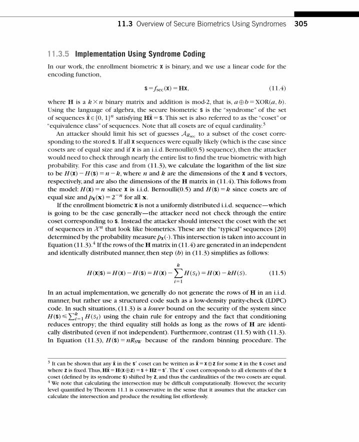
11.3 Overview of Secure Biometrics Using Syndromes 305
11.3.5 Implementation Using Syndrome Coding
In our work, the enrollment biometric x is binary, and we use a linear code for theencoding function,
s� fsec(x)�Hx, (11.4)
where H is a k�n binary matrix and addition is mod-2, that is, a⊕b�XOR(a, b).Using the language of algebra, the secure biometric s is the “syndrome” of the setof sequences x∈{0, 1}n satisfying Hx �s. This set is also referred to as the “coset” or“equivalence class”of sequences. Note that all cosets are of equal cardinality.3
An attacker should limit his set of guesses ARsec to a subset of the coset corre-sponding to the stored s. If all x sequences were equally likely (which is the case sincecosets are of equal size and if x is an i.i.d. Bernoulli(0.5) sequence), then the attackerwould need to check through nearly the entire list to find the true biometric with highprobability. For this case and from (11.3), we calculate the logarithm of the list sizeto be H(x)�H(s)�n�k, where n and k are the dimensions of the x and s vectors,respectively, and are also the dimensions of the H matrix in (11.4). This follows fromthe model: H(x)�n since x is i.i.d. Bernoulli(0.5) and H(s)�k since cosets are ofequal size and px(x)�2�n for all x.
If the enrollment biometric x is not a uniformly distributed i.i.d. sequence—whichis going to be the case generally—the attacker need not check through the entirecoset corresponding to s. Instead the attacker should intersect the coset with the setof sequences in X n that look like biometrics. These are the “typical” sequences [20]determined by the probability measure px(·).This intersection is taken into account inEquation (11.3).4 If the rows of the H matrix in (11.4) are generated in an independentand identically distributed manner, then step (b) in (11.3) simplifies as follows:
H(x|s)�H(x)�H(s)�H(x)�
k∑i�1
H(si)�H(x)�kH(s). (11.5)
In an actual implementation, we generally do not generate the rows of H in an i.i.d.manner, but rather use a structured code such as a low-density parity-check (LDPC)code. In such situations, (11.3) is a lower bound on the security of the system sinceH(s)�
∑ki�1 H(si) using the chain rule for entropy and the fact that conditioning
reduces entropy; the third equality still holds as long as the rows of H are identi-cally distributed (even if not independent). Furthermore, contrast (11.5) with (11.3).In Equation (11.3), H(s)�nRSW because of the random binning procedure. The
3 It can be shown that any x in the s� coset can be written as x �x⊕z for some x in the s coset andwhere z is fixed. Thus, Hx �H(x⊕z)�sHz�s�. The s� coset corresponds to all elements of the scoset (defined by its syndrome s) shifted by z, and thus the cardinalities of the two cosets are equal.4 We note that calculating the intersection may be difficult computationally. However, the securitylevel quantified by Theorem 11.1 is conservative in the sense that it assumes that the attacker cancalculate the intersection and produce the resulting list effortlessly.

306 CHAPTER 11 Securing Biometric Data
assumptions of this procedure no longer hold when using linear codes to implementbinning.
It is informative to consider estimating (11.5). The second term, kH(s) is easy toestimate since it involves only the entropy of a marginal distribution. An estimationprocedure would be to encode many biometrics using different codes, construct amarginal distribution for s, and calculate the entropy of the marginal. Particularly, ifthe code alphabet is small (say binary), little data is required for a good estimate. Thefirst term H(x) is harder to estimate. Generally, we would need to collect a very largenumber of biometrics (if n is large) to have sufficient data to make a reliable estimate ofthe entropy of the n-dimensional joint distribution.Thus,the absolute level of securityis difficult to evaluate. However,the analysis provides a firm basis on which to evaluatethe comparative security between two systems.The H(x) term is common to both andcancels out in a calculation of relative security—the difference between the individualsecurities, which is kH(s)�k�H(s�).
11.4 IRIS SYSTEMThis section describes a prototype implementation of a secure biometrics systemfor iris recognition based on syndrome coding techniques. Experimental results onthe Chinese Academy of Sciences Institute of Automation (CASIA) database [21] arepresented.
11.4.1 Enrollment and Authentication
At enrollment, the system performs the following steps. Starting with an image of auser’s eye, the location of the iris is first detected, and the torus is then unwrappedinto a rectangular region. Next, a bank of Gabor filters are applied to extract a bitsequence.The Matlab implementation from [22] could be used to perform these steps.Finally, the extracted feature vector x is produced by discarding bits at certain fixedpositions that were determined to be unreliable.5 The resulting x � ffeat(b) consists ofthe most reliable bits; in our implementation 1806 bits are extracted. Finally, the bitstring x is mapped into the secure biometric s by computing the syndrome of x withrespect to a LDPC code. Specifically, a random parity-check matrix H is selected froma good low-rate degree distribution obtained via density evolution [23] and s�H ·x iscomputed.
To perform authentication,the decoder gdec(·, ·) repeats the detection,unwrapping,filtering,and least-reliable bit dropping processes.The resulting observation y is used as
5 Unreliable positions are those positions at which the bit values (0 or 1) are more likely to flipdue to the noise contributed by eyelids and eyelashes, and due to a slight misalignment in the radialorientation of the photographed images. The bit positions corresponding to the outer periphery ofthe iris tend to be less reliable than those in the interior. These bit positions can be determined fromthe training data.

11.4 Iris System 307
(a)
(b)
FIGURE 11.3
Sample bit sequences extracted from iris data. (a) Two sample measurements from one user;(b) two sample measurements from a second user.
the input to a belief propagation decoder that attempts to find a sequence s satisfyingH · s�s. If the belief propagation decoder succeeds, then the output s�gdec(s, y).Otherwise, an authentication failure (or false rejection) is declared, and the output ofgdec(s, y) is ∅.
Sample iris measurements from two different users are shown in Figure 11.3.The bitcorrelation between different samples of the same user and differences between sam-ples of different users are easily seen. It has also been observed that the bit sequencesextracted from the irises contain significant inter-bit correlation. Specifically, let pi, j
be the probability of an iris bit taking the value i followed by another bit with thevalue j. If the bits extracted from an iris were independent and identically distributed,one would expect pi, j �1/4 for all (i, j)∈{0, 1}2. Instead, the following probabilitieshave been measured from the complete dataset:
p0,0 �0.319, p0,1 �0.166, p1,0 �0.166, p1,1 �0.349
Ignoring the inter-bit memory would result in degraded performance. Therefore, thebelief propagation decoder is designed to exploit this source memory. Further detailscan be found in [24].
11.4.2 Experimental Results
The system is evaluated using the CASIA iris database [21]. The iris segmentationalgorithm that was implemented was only able to correctly detect the iris in 624out of 756 images [22, Chapter 2.4]. Since our emphasis is on the secure biometricsproblem and not on iris segmentation,experiments were performed with the 624 iristhat were segmented successfully. Furthermore, half of the iris images were used fortraining.

308 CHAPTER 11 Securing Biometric Data
0 20 40 60 80 100 1201
1.5
2
2.5
3
Rob
ustn
ess
[�lo
g 2 P
FR
]
Security [No. of bits]
Performance withno security
FIGURE 11.4
Performance result of 312 iris images from CASIA database. Horizontal axis represents security,while vertical axis plots robustness in terms of the probability of false rejection. The original lengthof the bit sequence extracted from an iris is n �1806, while the length of the syndrome is1806 � t bits, where t is plotted along the horizontal axis above. In fact, the actual number of bitsof security is smaller than t because of inter-bit correlation in iris biometrics. A detailedexplanation appears at the end of this section.
Figure 11.4 reports performance results for the 312 image test set from the CASIAiris database.The horizontal axis represents security,while the vertical axis representsthe probability of false rejection for a legitimate user. Better systems correspond topoints in the lower right, but as Theorem 11.1 shows theoretically and the figuredemonstrates,there is a trade-off between security and robustness. Specifically,if a rateR LDPC code is used, then s contains n(1�R) bits. Under the idealized model wherethe iris data consists of i.i.d. Bernoulli (0.5) bits, our approach yields approximately1806 ·R bits of security with confidence approaching 1. Increasing R yields highersecurity, but lower robustness, so the security-robustness region can be estimated byvarying this parameter.
Note that if the biometric is stored in the clear,there is a probability of false rejectionequal to 0.0012 (i.e., the leftmost point in the graph). Thus, it is shown that, relativeto an insecure scheme,with essentially no change in the probability of authenticationfailure the syndrome-based scheme achieves almost 50 bits of security.
Higher levels of security can be achieved if larger authentication error rates areallowed. As discussed in Section 11.3, the true level of security is more difficult toevaluate. Specifically, the original length of the bit sequence extracted from an irisin the system is 1806, and the length of the syndrome produced by our encoder is1806� t , where t is a point on the horizontal axis of Figure 11.4. If the originalbiometric is an i.i.d. sequence of Bernoulli(0.5) random bits, then the probability ofguessing the true biometric from the syndrome would be about 2�t (i.e., security of tbits). However,as discussed earlier in this section,there is significant inter-bit memory

11.5 Fingerprint System: Modeling Approach 309
in iris biometrics. In particular, if the source was a first-order Markov source withthe measured pi, j statistics, the entropy of an 1806-bit measurement is only 0.9166 �1806�1655 bits, or 90 percent of the true blocklength. Since 1806� t � 90 percentof 1806 for all reasonable values of PFR in Figure 11.4,this suggests that an attacker withunbounded computational resources might be able to determine the true syndromemore quickly than by randomly searching a key space of size 2t . That said, we are notaware of any computationally feasible methods of improving upon random guessing,and we believe that the estimated security provided here is still reasonable.
11.5 FINGERPRINT SYSTEM: MODELING APPROACHIn the previous section, we remarked on the difficulties caused by the correlationsbetween bits in an iris biometric.These problems were dealt with by explicitly includ-ing the correlations in a belief propagation decoder. For fingerprint data,such problemsare more severe. Models for fingerprint biometrics do not obviously map onto blocksof i.i.d. bits as would be ideal for a Slepian–Wolf LDPC code.We present two solutionsto this problem. In this section, a “modeling” solution is discussed, in which the rela-tionship between the enrollment biometric and the probe biometric is modeled as anoisy channel.The rest of this section describes a somewhat complex statistical factorgraph model for fingerprint data and corresponding graph-based inference decodingtechniques.
In Section 11.6, a second “transformation” approach is introduced, in which thefingerprint biometric is transformed, as well as possible, into a block of i.i.d. bits, andthen a standard LDPC code and decoder are used. Although these two approachesare described in detail for fingerprint biometrics, other biometrics will have a similardichotomy of possible approaches. For fingerprints, we have found that the transfor-mation approach gives better results and makes it easier to quantify the security ofthe system, but both approaches are worth understanding.
11.5.1 Minutiae Representation of Fingerprints
A popular method for working with fingerprint data is to extract a set of “minutiaepoints”and to perform all subsequent operations on them [25]. Minutiae points havebeen observed to be stable over many years. Each minutiae is a discontinuity in theridge map of a fingerprint, characterized by a triplet (x, y, �) representing its spatiallocation in two dimensions and the angular orientation. In the minutiae map M of afingerprint, M(x, y)�� if there is a minutiae point at (x, y) and M(x, y)�∅ (emptyset) otherwise. A minutiae map may be considered as a joint quantization and fea-ture extraction function that operates on the fingerprint image, that is, the output ofthe ffeat(·) box in Figure 11.1. In Figure 11.5, the minutiae map is visualized using amatrix as depicted in the right-hand plot,where a 1 simply indicates the presence of aminutiae at each quantized coordinate. In this figure,as well as in the model describedthroughout the rest of this section, the � coordinate of the minutiae is ignored.

310 CHAPTER 11 Securing Biometric Data
1 1111
1 1 111
1 1 1 1 1
11
1 111 1 1 1 1 1
111111
1
Minutiaefeature
extraction
FIGURE 11.5
Fingerprint and extracted feature vector.
It is noted that different fingerprints usually have different numbers of minutiae.Furthermore, the number and location of minutiae could vary depending on the par-ticular extraction algorithm that is used. For some applications, it could be importantto account for such factors in addition to typical differences between fingerprintmeasurements, which will be discussed further in the next subsection. In the workdescribed here, the enrollment feature vector x is modeled as a Bernoulli i.i.d.randomvector.
11.5.2 Modeling the Movement of Fingerprint Minutiae
In the following, a model for the statistical relationship py|x(y|x) between the enroll-ment biometric and the probe biometric is described.This model captures three maineffects: (1) movement of enrollment minutiae when observed the second time in theprobe,(2) deletions,that is,minutiae observed at enrollment,but not during probe,and(3) insertions,that is,“spurious”minutiae observed in probe but not during enrollment.
Figure 11.6 depicts these three mechanisms in turn. First, minutiae observed atenrollment are allowed to jitter slightly around their locations in the enrollment vectorwhen registered the second time in the probe.This movement is modeled within a localneighborhood, where up to three pixels in either the horizontal or vertical direction(or both) could be accounted for. The size of the local neighborhood depends on theresolution of the minutiae map and how coarsely it is quantized. Second, a minutiaepoint may be registered in the enrollment reading but not in the probe. Or a minutiaepoint may be displaced beyond the local neighborhood defined by the movementmodel. Both count as “deletions.” Finally, minutiae points that are not observed atenrollment, but may be in the probe vector, are termed insertions.
The statistical model is formalized using a factor graph [26] as shown in Figure 11.7.The presence of a minutiae point at position t , t ∈{1, 2, . . . , n} in the enrollmentgrid is represented by the binary random variable x t that takes on the value x t �1

11.5 Fingerprint System: Modeling Approach 311
An enrollment minutiae’slocation may jitterlocally
An enrollment minutiaemay not appear in probe(deletion)
A minutiae may appearin probe but wasn’tthere at enrollment(insertion)
FIGURE 11.6
Statistical model of fingerprints corresponding to local movement, deletion, and insertion.
only if a minutiae is present during enrollment.6 For simplicity, the figure shows aone-dimensional movement model. All experimental results use a two-dimensionalmovement model.
The decoder observes two vectors: the probe biometric y i for i∈{1, 2, . . . , n} ands j for j∈{1, 2, . . . , k}.The decoder’s objective is to estimate the hidden x t enrollmentvariables.
The factor graph breaks down into three pieces. At the bottom of Figure 11.7 isthe code graph representing the H matrix (cf. (11.4)) that maps x into s. At the topof Figure 11.7 is the observation y. In between x and y is our model of movement,
6 Note that t indexes a position in the two-dimensional field of possible minutiae locations. Theparticular indexing used (e.g., raster-scan) is immaterial. The product of the number of rows and thenumber of columns equals n.

312 CHAPTER 11 Securing Biometric Data
Minutiaeinsertion/deletion/movementmodel
Estimate ofenrollmentbiometric
LDPCcodegraph
Probe biometric
Syndrome
FIGURE 11.7
Factor graph of the minutiae movement model.
deletion, and insertion. Each circle in the figure represents a variable node eitherobserved (s and y) or unobserved (x, h, and z) that needs to be estimated. The vectorh is a vector of binary variables, each indicating the current belief (at a given pointin the decoding process) whether an enrollment minutiae at position t is deleted.If a probe minutiae is observed at position t (i.e., y t �1), then z t indicates the cur-rent beliefs of what enrollment locations the minutiae might have come from andzN (t) �{z i|i∈N (t)} are the set of these variables in the neighborhood of enrollmentposition t .
The constraints between the variables and the priors that define the joint proba-bility function of all system variables are represented by the polygon factor nodes.Theconstraints enforced by each are as follows. The prior on x t is p�(xt). The prior ondeletion is p�(ht).The prior on insertion is p (zt).The constraint that each enrollmentminutiae is paired with only a single probe minutiae is enforced by the function node�. In other words,� says that an enrollment minutiae can move to at most one positionin the probe, or it can be deleted. Finally, in the reverse direction,♦ constrains probeminutiae either to be paired with only a single enrollment minutiae or to be explainedas an insertion. For a more detailed discussion of the statistical model, see [27, 28].The complete statistical model of the enrollment and probe biometrics is
px,y(x, y)�px(x)py|x(y|x)�∑{hi}
∑{zi}
∏t
p�(xt)p�(ht)p (zt)�(xt , ht , zN (t))♦(zt , yt).

11.5 Fingerprint System: Modeling Approach 313
The above statistical model of the biometrics is combined with the code graph. Thisyields the complete model used for decoding px,y,s(x, y, s)�px,y(x, y)
∏j ⊕(sj, x),
where⊕(sj, x) indicates that the mod-2 sum of sj and the xi connected to syndrome jby the edges of the LDPC code is constrained to equal zero.A number of computationaloptimizations must be made for inference to be tractable in this graph. See [27, 28]for details.
11.5.3 Experimental Evaluation of Security and Robustness
We use a proprietary Mitsubishi Electric (MELCO) database to evaluate our techniques.The database consists of a set of fingerprint measurements with roughly 15 measure-ments per finger. One measurement is selected as the enrollment, while decoding isattempted, with the remaining 14 serving as probes. The locations of the minutiaepoints were quantized to reside in a 70�100 grid,resulting in a blocklength n�7000.
The mean and standard deviation of movement,deletions ( pD),and insertions ( pI)for the MELCO dataset are plotted in Figure 11.8.The label d �1 labels the probabilitythat an enrollment minutiae moved a distance of one pixel in either the vertical orhorizontal direction, or both (i.e., the max- or �-norm). These parameters are used toset parameter values in the factor graph.
A summary of test results is given in Table 11.1. Results are categorized by thenumber of minutiae in the enrollment print. To first order, this is a measure of therandomness of the enrollment biometric. As an estimate of H(x), we say that if afingerprint has, for example,33 minutiae, its entropy is 7000�HB(33/7000)�7000�0.0432�302. Each row in the table tabulates results for enrollment biometrics, withthe number of minutiae indicated in the first column. The second column indicateshow many users had that number of minutiae in their enrollment biometric.
In the security-robustness trade-off developed in Section 11.3.3, it was found thatholding all other parameters constant (in particular, the rate of the error-correctingcode), security should increase and robustness decrease as the biometric entropy
d = 0 d = 1 d = 2 d = 3 pD pI0
0.1
0.2
0.3
0.4
Priors
Pro
babi
lity
Mean
Stnd dev
FIGURE 11.8
Empirical movement statistics.
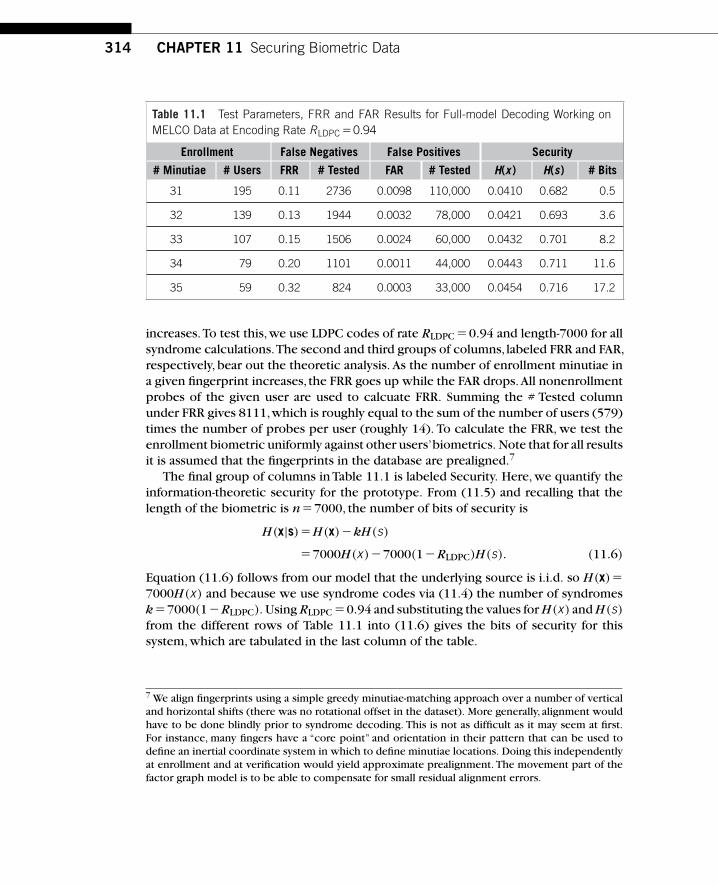
314 CHAPTER 11 Securing Biometric Data
Table 11.1 Test Parameters, FRR and FAR Results for Full-model Decoding Working onMELCO Data at Encoding Rate RLDPC �0.94
Enrollment False Negatives False Positives Security
# Minutiae # Users FRR # Tested FAR # Tested H(x ) H(s) # Bits
31 195 0.11 2736 0.0098 110,000 0.0410 0.682 0.5
32 139 0.13 1944 0.0032 78,000 0.0421 0.693 3.6
33 107 0.15 1506 0.0024 60,000 0.0432 0.701 8.2
34 79 0.20 1101 0.0011 44,000 0.0443 0.711 11.6
35 59 0.32 824 0.0003 33,000 0.0454 0.716 17.2
increases.To test this,we use LDPC codes of rate RLDPC �0.94 and length-7000 for allsyndrome calculations.The second and third groups of columns, labeled FRR and FAR,respectively, bear out the theoretic analysis. As the number of enrollment minutiae ina given fingerprint increases, the FRR goes up while the FAR drops. All nonenrollmentprobes of the given user are used to calcuate FRR. Summing the # Tested columnunder FRR gives 8111,which is roughly equal to the sum of the number of users (579)times the number of probes per user (roughly 14). To calculate the FRR, we test theenrollment biometric uniformly against other users’biometrics. Note that for all resultsit is assumed that the fingerprints in the database are prealigned.7
The final group of columns in Table 11.1 is labeled Security. Here, we quantify theinformation-theoretic security for the prototype. From (11.5) and recalling that thelength of the biometric is n�7000, the number of bits of security is
H(x|s)�H(x)�kH(s)
�7000H(x )�7000(1�RLDPC)H(s). (11.6)
Equation (11.6) follows from our model that the underlying source is i.i.d. so H(x)�7000H(x ) and because we use syndrome codes via (11.4) the number of syndromesk�7000(1�RLDPC). Using RLDPC �0.94 and substituting the values for H(x ) and H(s)
from the different rows of Table 11.1 into (11.6) gives the bits of security for thissystem, which are tabulated in the last column of the table.
7 We align fingerprints using a simple greedy minutiae-matching approach over a number of verticaland horizontal shifts (there was no rotational offset in the dataset). More generally, alignment wouldhave to be done blindly prior to syndrome decoding. This is not as difficult as it may seem at first.For instance, many fingers have a “core point” and orientation in their pattern that can be used todefine an inertial coordinate system in which to define minutiae locations. Doing this independentlyat enrollment and at verification would yield approximate prealignment. The movement part of thefactor graph model is to be able to compensate for small residual alignment errors.

11.6 Fingerprint System: Transformation Approach 315
11.5.4 Remarks on the Modeling Approach
This section describes a secure fingerprint biometrics scheme in which an LDPC codegraph was augmented with a second graph that described the “fingerprint channel”relating the enrollment to the probe biometric. A number of improvements are pos-sible. For example, we implement an LDPC code designed for a binary symmetricchannel (BSC). This design is not tuned to the fingerprint channel model. One pos-sible improvement is to refine the design of the LDPC to match that channel. Ingeneral, however, while the “fingerprint channel” is a reasonable model of the vari-ations between the enrollment and probe fingerprints, the techniques developedare specific to the feature set, and the resulting inference problem is complex andnonstandard. In addition, higher levels of security are desired. For these reasons, wetake a different approach in the next section that aims to redesign the feature extrac-tion algorithm to yield biometric features that are well matched to a standard problemof syndrome decoding.
11.6 FINGERPRINT SYSTEM: TRANSFORMATIONAPPROACH
In this section we aim to revamp the feature extraction algorithm to producebiometric features with statistics well matched to codes designed for the BSC.Since the construction of LDPC codes for the BSC is a deeply explored and well-understood topic, we are immediately able to apply that body of knowledge to thesecure biometrics problem. We believe this is a more promising approach, in partbecause the design insights we develop can be applied to building transforms forother biometric modalities. In contrast, the biometric channel model developed inSection 11.5.2 is specific to fingerprints and minutiae points. In addition,the system wedescribe for fingerprints in this section achieves a higher level of information-theoreticsecurity.
The transform-based secure fingerprint biometrics scheme is depicted inFigure 11.9. In Section 11.5, the function ffeat(·) extracted minutiae maps from theenrollment and probe fingerprints. Here, in addition to minutiae extraction, the ffeat(·)box also encompasses a feature transformation algorithm that converts the 2D minu-tiae maps to 1D binary feature vectors. The central idea is to generate binary featurevectors that are i.i.d. Bernoulli(0.5), independent across different users but such thatdifferent measurements of the same user are related by a binary symmetric channelwith crossover probability p (BSC-p), where p is much smaller than 0.5. This is oneof the standard channel models for LDPC codes, and therefore standard LDPC codescan be used for Slepian–Wolf coding of the feature vectors. We emphasize that thefeature transformation we now present is made public and is not assumed to provideany security—in contrast to some of the transform-based techniques discussed inSection 11.2.

316 CHAPTER 11 Securing Biometric Data
Alignmentand
Minutiaeextraction
Alignmentand
Minutiaeextraction
ffeat(b) fsec(x)
ffeat(b9) gdec(y, s)
Enrollmentfingerprint
Probefingerprint
Extractbinaryfeaturevectors
Extractbinaryfeaturevectors
Syndromeencoding
Syndromedatabase
Syndromedecoding
yes
yes
no
no
Accessdenied
Accessgranted
Accessdenied
y
x
s
s
' s. t.fsec( ) 5s ?
fhash( ) 5fhash(x) ?
b
b9
x
xx
FIGURE 11.9
Robust feature extraction is combined with syndrome coding to build a secure fingerprintbiometrics system.
11.6.1 Desired Statistical Properties of Feature Vectors
We aim to have a feature vector that possesses the following properties:
1. A bit in a feature vector representation is equally likely to be a 0 or a 1. Thus,
Pr{x i �0}�Pr{x i �1}�1/2 and H(x i)�1 bit for all i∈I �{1, 2, . . . , n}.
2. Different bits in a given feature vector are independent of each other, so that agiven bit provides no information about any other bit.Thus,the pairwise entropyH(x i, x j)�H(x i)H(x j)�2 bits for all i �� j where i, j ∈ I.This property,alongwith the first property, ensures that the feature vector cannot be compressedfurther; that is, it presents the maximum possible uncertainty for an attackerwho has to guess a portion of a feature vector given some other portion.
3. Feature vectors x and y from different fingers are independent of each other, sothat one person’s feature vector provides no information about another person’sfeature vector.Thus,the pairwise entropy H(x i, y j)�H(x i)H( y j)�2 bits forall i, j ∈ I.
4. Feature vectors x and x� obtained from different readings of the same finger arestatistically related by a BSC-p. If p is small, it means that the feature vectors arerobust to repeated noisy measurements with the same finger.Thus,H(x �i|x i)�H( p) for all i ∈ I.
The last property ensures that a Slepian–Wolf code with an appropriately chosenrate makes it possible to estimate the enrollment biometric when provided withfeature vectors from the enrollee. At the same time, the chosen coding rate makes itextremely difficult (practically impossible) to estimate the enrollment biometric whenprovided with feature vectors from an attacker or from a different user. To show thatthe resulting biometrics system is information-theoretically secure, proceed just as in
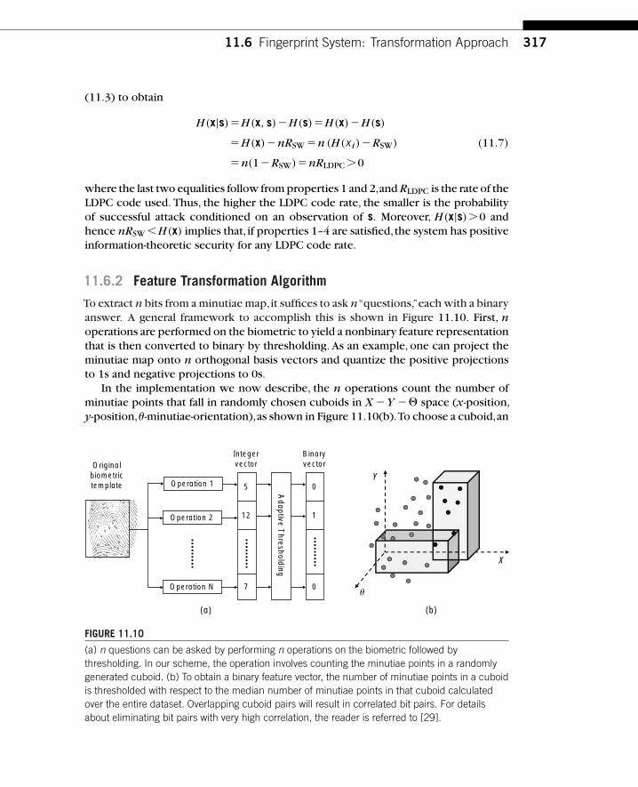
11.6 Fingerprint System: Transformation Approach 317
(11.3) to obtain
H(x|s)�H(x, s)�H(s)�H(x)�H(s)
�H(x)�nRSW �n (H(x i)�RSW) (11.7)
�n(1�RSW)�nRLDPC �0
where the last two equalities follow from properties 1 and 2,and RLDPC is the rate of theLDPC code used. Thus, the higher the LDPC code rate, the smaller is the probabilityof successful attack conditioned on an observation of s. Moreover, H(x|s)�0 andhence nRSW �H(x) implies that, if properties 1–4 are satisfied,the system has positiveinformation-theoretic security for any LDPC code rate.
11.6.2 Feature Transformation Algorithm
To extract n bits from a minutiae map,it suffices to ask n“questions,”each with a binaryanswer. A general framework to accomplish this is shown in Figure 11.10. First, noperations are performed on the biometric to yield a nonbinary feature representationthat is then converted to binary by thresholding. As an example, one can project theminutiae map onto n orthogonal basis vectors and quantize the positive projectionsto 1s and negative projections to 0s.
In the implementation we now describe, the n operations count the number ofminutiae points that fall in randomly chosen cuboids in X �Y �� space (x-position,y-position,�-minutiae-orientation),as shown in Figure 11.10(b).To choose a cuboid,an
Y
X
�
Originalbiometrictemplate Operation 1
Integervector
Adaptive T
hresholding
Binaryvector
Operation 2
Operation N 7
12 1
5 0
0
(a) (b)
FIGURE 11.10
(a) n questions can be asked by performing n operations on the biometric followed bythresholding. In our scheme, the operation involves counting the minutiae points in a randomlygenerated cuboid. (b) To obtain a binary feature vector, the number of minutiae points in a cuboidis thresholded with respect to the median number of minutiae points in that cuboid calculatedover the entire dataset. Overlapping cuboid pairs will result in correlated bit pairs. For detailsabout eliminating bit pairs with very high correlation, the reader is referred to [29].

318 CHAPTER 11 Securing Biometric Data
origin is selected uniformly at random in X �Y �� space, and the dimensions alongthe three axes are also chosen at random.
Next, define the threshold as the median of the number of minutiae points in thechosen cuboid, measured across the complete training set. A similar method is usedfor face recognition in [30]. The threshold value may differ for each cuboid basedon its position and volume. If the number of minutiae points in a randomly generatedcuboid exceeds the threshold,then a 1-bit is appended to the feature vector;otherwisea 0-bit is appended. We consider the combined operation of (a) generating a cuboidand (b) thresholding as equivalent to posing a question with a binary answer. With nsuch questions we get an n-bit feature vector.
The simplest way to generate feature vectors is to use the same questions for allusers. In the sequel,we consider a more advanced approach in which the questions areuser-specific.The rationale behind using user-specific questions is that some questionsare more robust (reliable) than others. In particular,a question is robust if the numberof minutiae points in a cuboid is much greater or much less than the median calculatedover the entire dataset.Thus,even if there is spurious insertion or deletion of minutiaepoints when a noisy measurement of the same fingerprint is provided at a later time,the answer to the question (0 or 1) is less likely to change. On the other hand, if thenumber of minutiae points is close to the median, the 0 or 1 answer to that questionis less reliable. Thus, more reliable questions result in a BSC-p intra-user channel withlow p. Different users have a different set of robust questions, and we propose touse these while constructing the feature vector. We emphasize that for the purposesof security analysis, the set of questions used in the system is assumed public. Anattacker who steals a set of syndromes and poses falsely as a user will be given theset of questions appropriate to that user. Our security analysis is not based in any wayon the obscurity of the questions,but rather on the information-theoretic difficulty ofrecovering the biometric given only the stolen syndromes.
For a given user i, the average number of minutiae points mi,j in a given cuboidCj is calculated over repeated noisy measurements of the same fingerprint. Let mj and�j be the median and standard deviation of the number of minutiae points in Cj overthe dataset of all users.Then, let �i,j �(mi,j �mj)/�j . The magnitude, |�i,j | is directlyproportional to the robustness of the question posed by cuboid Cj for user i.The signof �i,j determines whether the cuboid Cj should be placed into L0,i ,a list of questionswith a 0 answer for user i, or into L1,i , a list of questions with a 1 answer for user i.Both of these lists are sorted in the decreasing order of |�i,j |. Now,a fair coin is flippedto choose between L0,i and L1,i and the question at the top of the chosen list is storedon the device.After n coin flips,approximately n/2 of the most robust questions fromeach list will be stored on the device.This process is repeated for each enrolled user i.
11.6.3 Experimental Evaluation of Security and Robustness
In the following experiments,we use the same Mitsubishi Electric fingerprint databaseas described in the previous section, which contains minutiae maps of 1035 fin-gers with 15 fingerprint samples taken from each finger. The average number of

11.6 Fingerprint System: Transformation Approach 319
minutiae points in a single map is approximately 32. As before, all fingerprints areprealigned. To measure the extent to which the desired target statistical properties inSection 11.6.1 are achieved, we examine the feature vectors obtained from the minu-tiae maps according to the method described in Section 11.6.2. The n most robustquestions were selected to generate the feature vectors, with n ranging from 50 to350. Figure 11.11 shows the statistical properties of the feature vectors for n�150.Asshown in Figure 11.11(a), the histogram of the average number of 1-bits in the featurevectors is clustered around n/2�75. Figure 11.11(b) shows that the pairwise entropymeasured between bits of different users is very close to 2 bits. Thus, bits are nearlypairwise independent and nearly uniformly distributed, approximating property 1.
In order to measure the similarity or dissimilarity of two feature vectors, the nor-malized Hamming distance (NHD) is used. The NHD between two feature vectors xand y, each having length n, is calculated as follows:
NHD(x, y)�1
n
n∑i�1
(xi⊕yi)
where ⊕ is summation modulo 2. The plot of Figure 11.12(a) contains three histo-grams:(1) the intra-user variation is the distribution of the average NHD measured pair-wise over 15 samples of the same finger, (2) the inter-user variation is the distributionof the NHD averaged over all possible pairs of users,each with his own specific set ofquestions, and (3) the attacker variation is the NHD for the case in which an attackerattempts to identify himself as a given user i,while using a different fingerprint j �� i butusing the 150 robust questions of user i.As seen in the figure,there is a clean separationbetween the intra-user and inter-user NHD distributions, and a small overlap betweenthe intra-user and attacker distributions. One way to ascertain the effectiveness of thefeature vectors is to choose different threshold NHDs in Figure 11.12(a) and plotthe intra-user NHD against the inter-user NHD.This trade-off between intra-user NHD
30 40 50 60 70
(a) (b)
80 90 100 110 1200
50
100
150
200
250
300
350
400
450
Number of 1’s in the transformed feature vectors
Num
ber
of fe
atur
e ve
ctor
s
1.985 1.99 1.995 20
500
1000
1500
2000
2500
3000
3500
4000
4500
5000
Pairwise entropy
Num
ber
of p
airs
FIGURE 11.11
(a) Histogram of the number of ones in the feature vectors for n = 150 is clustered aroundn/2 � 75. (b) The pairwise entropy measured across all pairs and all users is very close to 2 bits.
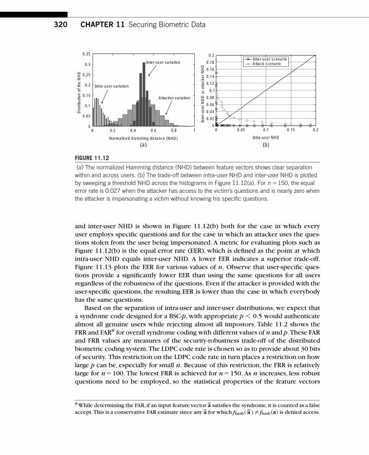
320 CHAPTER 11 Securing Biometric Data
0 0.05 0.1 0.15 0.20
0.02
0.04
0.06
0.08
0.1
0.12
0.14
0.16
0.18
0.2
Intra-user NHD
Inte
r-us
er N
HD
or
atta
cker
NH
D
Inter-user scenarioAttack scenario
0 0.2 0.4 0.6 0.8 10
0.05
0.1
0.15
0.2
0.25
0.3
0.35
Normalized Hamming distance (NHD)
Dis
trib
utio
n of
the
NH
D
Attacker variation
Inter-user variation
Intra-user variation
(a) (b)
FIGURE 11.12
(a) The normalized Hamming distance (NHD) between feature vectors shows clear separationwithin and across users. (b) The trade-off between intra-user NHD and inter-user NHD is plottedby sweeping a threshold NHD across the histograms in Figure 11.12(a). For n �150, the equalerror rate is 0.027 when the attacker has access to the victim’s questions and is nearly zero whenthe attacker is impersonating a victim without knowing his specific questions.
and inter-user NHD is shown in Figure 11.12(b) both for the case in which everyuser employs specific questions and for the case in which an attacker uses the ques-tions stolen from the user being impersonated. A metric for evaluating plots such asFigure 11.12(b) is the equal error rate (EER), which is defined as the point at whichintra-user NHD equals inter-user NHD. A lower EER indicates a superior trade-off.Figure 11.13 plots the EER for various values of n. Observe that user-specific ques-tions provide a significantly lower EER than using the same questions for all usersregardless of the robustness of the questions. Even if the attacker is provided with theuser-specific questions, the resulting EER is lower than the case in which everybodyhas the same questions.
Based on the separation of intra-user and inter-user distributions, we expect thata syndrome code designed for a BSC-p, with appropriate p � 0.5 would authenticatealmost all genuine users while rejecting almost all impostors. Table 11.2 shows theFRR and FAR8 for overall syndrome coding with different values of n and p.These FARand FRR values are measures of the security-robustness trade-off of the distributedbiometric coding system.The LDPC code rate is chosen so as to provide about 30 bitsof security. This restriction on the LDPC code rate in turn places a restriction on howlarge p can be, especially for small n. Because of this restriction, the FRR is relativelylarge for n�100. The lowest FRR is achieved for n�150. As n increases, less robustquestions need to be employed, so the statistical properties of the feature vectors
8 While determining the FAR,if an input feature vector a satisfies the syndrome,it is counted as a falseaccept.This is a conservative FAR estimate since any a for which fhash( a ) �� fhash(a) is denied access.

11.6 Fingerprint System: Transformation Approach 321
0 50 100 150 200 250 300 350 4000
0.01
0.02
0.03
0.04
0.05
0.06
0.07
Length of the binary feature vector, n
Equ
al e
rror
rat
esAll users have identical questions
Everyone uses their own user-specific questions
Attacker steals and applies user-specific questions
FIGURE 11.13
User-specific questions result in lower EER than common questions, even if the user-specificquestions are given to the attacker.
Table 11.2 Syndrome Coding with an Appropriate LDPC Code Gives an Information-theoretically Secure Biometrics System with Low FRR and Extremely Low FAR
n BSC Crossover RLDPC FRR after FAR after No. of BitsProbability, p Syndrome Coding Syndrome Coding of Security
100 0.1 0.3 0.23 0.0001 30
150 0.13 0.2 0.11 0.0001 30
200 0.2 0.15 0.14 0.0014 30
250 0.2 0.125 0.15 0.0035 31.25
diverge from those in Section 11.6.1. Thus, the FRR increases again when n becomestoo large.
Compare the FRR, FAR, and number of bits of security reported in Table 11.2 withthose reported in Section 11.5. We observe that the FRR and FAR are comparable,but the transformation approach described in this section provides a higher numberof bits of security compared to the model-based approach of Section 11.5 (see finalcolumn of Table 11.1). The security-robustness trade-off has improved because thestatistical properties of the transformed feature vectors are intentionally matched tothe standard LDPC code for a binary symmetric channel.

322 CHAPTER 11 Securing Biometric Data
11.7 SUMMARYThis chapter demonstrates that the principles of distributed source coding can besuccessfully applied to the problem of secure storage of biometrics. A Slepian–Wolfframework is used to store a secure version of the biometric template data collectedat enrollment and to recover the enrollment template at authentication. The trade-offbetween security and robustness in this framework is formally defined and discussed,and sample implementations based on iris and fingerprint data validate the theory.
Although iris data tends to be relatively well behaved and exhibits easily modeledsample-to-sample variability (both between samples of the same user and across users),the same cannot be said of fingerprints. It is shown that the fingerprint noise channelis far removed from the standard bit-flipping (e.g., BSC) channel model of communi-cation systems. The design of a secure system for such biometric modalities thereforerequires additional attention. Two approaches are discussed. The first design is basedon using a sparse binary matrix representation of minutiae locations and developinga model of minutiae movement that can be combined with a graphical representationof a linear code. Although this approach does not yet yield satisfactory performancein terms of security and robustness, it does reveal various factors that affect perfor-mance and provides valuable insight that motivates the transform-based approach ofSection 11.6.
In the latter approach, a transform is designed to convert the fingerprint featureset into a binary vector with desirable statistical properties, in the sense of being wellmatched to well-understood channel coding problems. The resultant design yieldsvery low false-acceptance and false-rejection rates. Furthermore, it ensures operationwell into the information-theoretically secure region. We believe this to be a powerfulconcept that will allow extension of this framework to other biometric data. It mayalso prove useful in resolving performance issues with other Slepian–Wolf-inspiredsystems.
Besides further improving security and robustness,there are a number of additionalopen research issues. As one example, the designs presented in this chapter assumedthat the biometric data is prealigned. In practice,this is not the case,and biometric datamust be aligned blindly, that is, without access to other reference data. One researchtrajectory is the design of such algorithms. An alternative to blind alignment is thedesign of a translation- and rotation-invariant feature set.A second aspect of the securebiometrics that has not received much attention concerns multibiometric systems. Inthese systems multiple biometrics are collected at enrollment and verification—suchas both iris and fingerprint.The measurements are fused to improve overall robustnessand security. This particular combination and some encouraging results are presentedby Nandakumar in [31]. However, the topic has yet to be studied in the context of aSlepian–Wolf coding system.
As the use of biometrics becomes more widespread, the incentive to attack bio-metric systems will grow. Assuming the technology for securing biometric data issufficiently mature, it would be natural to standardize the template protection design.

References 323
Such work is within the scope of ISO/IEC JTC1/SC37, which is an international stan-dardization committee on biometrics. Open issues to be handled by this committeewould range from quantifying the inherent entropy and security limits of biometricdata to remote authentication scenarios.
As a final note,the biometric system described in this chapter is one example wherea noisy version of an original signal is available at the decoder for the purpose ofauthentication.This type of setup is extended to the problem of image authenticationfollowing similar principles [32]. We believe that there are many such applications inwhich the principles of distributed source coding can be applied.
REFERENCES[1] D. Slepian and J. K. Wolf, “Noiseless Coding of Correlated Information Sources,” IEEE Trans.
Information Theory, pp. 471–480, July 1973.
[2] N. Ratha, J. Connell, R. Bolle, and S. Chikkerur, “Cancelable Biometrics: A Case Study inFingerprints,” in Intl. Conf. on Pattern Recognition, Hong Kong, Septemper 2006, pp. 370–373.
[3] N. K. Ratha, S. Chikkerur, J. H. Connell, and R. M. Bolle, “Generating Cancelable FingerprintTemplates,” IEEE Transactions on Pattern Analysis and Machine Intelligence, vol. 29, no. 4,pp. 561–572, April 2007.
[4] K. Sakata, T. Maeda, M. Matsushita, K. Sasakawa, and H. Tamaki, “Fingerprint AuthenticationBased on Matching Scores with Other Data,” in Lecture Notes in Computer Science, ser. LNCS,vol. 3832, 2005, pp. 280–286.
[5] A. Teoh,A. Gho, and D. Ngo,“Random Multispace Quantization as an Analytic Mechanism forBiohashing of Biometric and Random Identity Inputs,” IEEE Transactions on Pattern Analysisand Machine Intelligence, vol. 28, no. 12, pp. 1892–1901, December 2006.
[6] R. Ahlswede and I. Csiszar,“Common Randomness in Information Theory and Cryptography I:Secret Sharing,” IEEE Trans. Information Theory, vol. 39, no. 4, pp. 1121–1132, July 1993.
[7] G. I. Davida, Y. Frankel,and B. J. Matt,“On Enabling SecureApplications through Off-line Biomet-ric Identification,” in Proc. IEEE Symposium on Security and Privacy, Oakland, CA, May 1998,pp. 148–157.
[8] A. Juels and M. Wattenberg,“A Fuzzy Commitment Scheme,” in CCS ’99: Proceedings of the 6thACM Conference on Computer and Communications Security. New York: ACM Press, 1999,pp. 28–36.
[9] F. Hao, R. Anderson, and J. Daugman, “Combining Cryptography with Biometrics Effectively,”University of Cambridge, Tech. Rep. UCAM-CL-TR-640, July 2005.
[10] A. Juels and M. Sudan, “A Fuzzy Vault Scheme,” in Proc. International Symposium on Infor-mation Theory, Lausanne, Switzerland, July 2002, p. 408.
[11] T. C. Clancy, N. Kiyavash, and D. J. Lin, “Secure Smartcard-based Fingerprint Authentication,”in ACM SIGMM Workshop on Biometrics Methods and Applications, Berkeley, CA, November2003, pp. 45–52.
[12] S. Yang and I. M. Verbauwhede,“Secure Fuzzy Vault-based Fingerprint Verification System,” inAsilomar Conference on Signals, Systems, and Computers, vol. 1, Asilomar, CA, November2004, pp. 577–581.
[13] U. Uludag, S. Pankanti, and A. K. Jain, “Fuzzy Vault for Fingerprints,” in Audio- and Video-Based Biometric Person Authentication, 5th International Conference, AVBPA 2005, Hilton

324 CHAPTER 11 Securing Biometric Data
Rye Town, NY, USA, July 20–22, 2005, Proceedings, ser. Lecture Notes in Computer Science,vol. 3546. Springer, 2005.
[14] K. Nandakumar, A. K. Jain, and S. Pankanti, “Fingerprint-based Fuzzy Vault: Implementationand Performance,” IEEE Transactions on Information Forensics and Security, vol. 2, no. 4,pp. 744–757, December 2007.
[15] D. Maio, D. Maltoni, J. Wayman, and A. K. Jain, “FVC2002: Second Fingerprint VerificationCompetition,” in International Conference on Pattern Recognition, Quebec, Canada,August2002, pp. 811–814.
[16] U. Uludag, S. Pankanti, S. Prabhakar, and A. K. Jain, “Biometric Cryptosystems: Issues andChallenges,”Proceedings of the IEEE, vol. 92, no. 6, pp. 948–960, June 2004.
[17] A. K. Jain, S. Pankanti, S. Prabhakar, L. Hong, and A. Ross, “Biometrics: A Grand Challenge,”In Proc. International Conference on Pattern Recognition, vol. 2, Cambridge, UK, August2004, pp. 935–942.
[18] T. M. Cover,“A Proof of the Data CompressionTheorem of Slepian andWolf for Ergodic Sources,”IEEE Trans. Inform.Theory, vol. 21, no. 2, pp. 226–228, March 1975.
[19] R. G. Gallager, “Source Coding with Side Information and Universal Coding,” MassachusettsInstitute of Tech.,Tech. Rep. LIDS P-937, 1976.
[20] T. M. Cover and J. A. Thomas, Elements of Information Theory. New York: Wiley, 1991.
[21] “CASIA Iris Image Database collected by Institute ofAutomation,ChineseAcademy of Sciences.”[Online]. Available: http://www.sinobiometrics.com.
[22] L. Masek,“Recognition of Human Iris Patterns for Biometric Identification,” Bachelor’s Thesis,University of Western Australia, 2003.
[23] T. J. Richardson,M. A. Shokrollahi, and R. L. Urbanke,“Design of Capacity-Approaching IrregularLow-density Parity Check Codes,” IEEE Transactions on Information Theory, vol. 47, no. 2,pp. 619–637, February 2001.
[24] E. Martinian, S. Yekhanin, and J. S. Yedidia,“Secure Biometrics via Syndromes,” in Allerton Conf.,Monticello, IL, September 2005, pp. 1500–1510.
[25] A. K. Jain,L. Hong,and R. Bolle,“On-line fingerprint verification,” IEEE Transactions on PatternAnalysis and Machine Intelligence, vol. 19, no. 4, pp. 302–314, April 1997.
[26] F. R. Kschischang, B. J. Frey, and H. Loeliger,“Factor Graphs and the Sum-Product Algorithm,”IEEE Transactions on Information Theory, vol. 47, no. 2, pp. 498–519, February 2001.
[27] S. C. Draper, A. Khisti, E. Martinian, A. Vetro, and J. S. Yedidia, “Secure Storage of FingerprintBiometrics Using Slepian–Wolf Codes,” in Inform. Theory and Apps. Work., UCSD, San Diego,CA, January 2007.
[28] , “Using Distributed Source Coding to Secure Fingerprint Biometrics,” in Int. Conf.Acoutics Speech Signal Proc., Honolulu, HI, April 2007, pp. II–(129–132).
[29] Y. Sutcu, S. Rane, J. S. Yedidia, S. C. Draper, and A. Vetro,“Feature Transformation for a Slepian-Wolf Biometric System Based on Error Correcting Codes,” in Computer Vision and PatternRecognition (CVPR) Biometrics Workshop, Anchorage, AK, June 2008.
[30] T. Kevenaar, G. Schrijen, M. V. der Veen, A. Akkermans, and F. Zuo, “Face Recognition withRenewable and Privacy Preserving Binary Templates,” Fourth IEEE Workshop on AutomaticIdentification Advanced Technologies, pp. 21–26, 2005.
[31] K. Nandakumar, “Multibiometric Systems:Fusion Strategies andTemplate Security,”Ph.D.Thesis,Michigan State University, 2008.
[32] Y. C. Lin,D.Varodayan,and B. Girod,“ImageAuthentication Based on Distributed Source Coding,”in International Conference on Image Processing, San Antonio,TX, September 2007.

Index
AAbsorption bands, 270Advanced Video Coding. See H.264/AVCArithmetic codes, 36, 227
overlapped and punctured, 151–152quasi-, 151–152
Availability, 295
BBayesian decision theory, 68Bennett assumptions, 73, 75BER. See Bit Error RateBerkeley WZ video codecs
comparison of early, 200–201at decoder
DCT and, 200hash checking of, 199motion search and, 199reconstruction and, 200syndrome, 199
at encoderblock classification of, 198–199, 198fhash generation of, 199quantization of, 198–199, 198fsyndrome coding of, 199transform of, 198, 198f
Bessel function, 164Binary symmetric channel (BSC), 133–134
codes, 315combinations, 139, 139f, 140
Binaural hearing aid configurationcoding strategies of, 179–180, 180frate-distortion trade-offs and, 180–185, 182f,
184f, 185fsetup of, 177–179, 178f, 179f
Binning, 133schemes, 134–135, 135fstrategy of, 10structured, 135
Biometric dataarchitectures and system security with,
295–296authentication and employment of, 299–300,
300fchapter organization and, 296Definition 11.1, 302introduction to, 294–296iris system and, 306–309, 306n5, 307f, 308f
notation of, 299objectives and motivation associated with,
294–295overview of secure, 299–306, 300f, 300nn1–2,
304f, 305n3performance measures of, 300–302related work associated with, 296–299security-robustness of, 300–304, 304fsummary on, 322–323Theorem 11.1, 303–304
Bit(s), 151. See also Bit Error Rate; Most significantbit-plane
number of, 125–126parity, 141-plane compression factor and DISCOVER
Wyner-Ziv video codecs, 225–227, 226f, 228fpunctured, 141–142rates, 225total rate, 185f
Bit Error Rate (BER), 139–140Blahut-Arimoto algorithm, 6BSC. See Binary symmetric channelButterfly support, 163–164
CCASIA. See Chinese Academy of Sciences Institute
of AutomationCentralized source coding, 4–9, 5f, 7f, 7t
Definition A.6, 25Definition A.7, 25Definition A.8, 25Definition A.9, 25Definition A.10, 25Definition A.11, 26definitions of, 16distributed v., 16Theorem 1.8 and, 17Theorem 1.9 and, 17–18, 17f
CEO. See Chief estimation officerChannel coding, 98, 140
joint source-, 22–23, 22fDefinition 1.1, 22Definition 1.2, 22Definition 1.3, 22Theorem 1.11 and, 22–23
practical code design based on, 133f, 134n1,135f, 136–139, 137f, 138f, 139f
SW and, 193, 201–202 325

326 Index
Characteristic graph G, 90, 93Chief estimation officer (CEO)
problems, 19rate-distortion function and, 21
Chinese Academy of Sciences Institute ofAutomation (CASIA), 306, 307–308, 308f
Chromatic graph G, 93CNM. See Correlation noise modelingCoast Guard
frames, 217, 217f, 220sequences, 220, 221f, 222f, 223
Code(s)BSC, 315convolutional, 137design based on channel coding, 133f, 134n1,
135f, 136–139, 137f, 138f, 139fHadamard, 297Huffman, 36LDPC, 143, 149, 201–202, 206, 211–213length, 151turbo, 139, 139f, 142f, 225words, 134, 137
Codingasymmetric, 90binary, 134centralized, 170–171, 171f, 172channel, 98, 140entropy, 35–37, 190gain, 41instantaneous, 94–95Intra, 196, 197Lloyd algorithm for distributed, 70, 70fmultiterminal, 170–171, 171fparadigms, 190performance, 288rates, 118sequences, 256–257, 257tsimple, 35spatially independent, 170–171, 171fsyndrome
of BerkeleyWZ video codecs at encoder,199implementation using, 305–306, 306nn3–4
transform, 190with vanishing small error, 90zero-error, 89–92
Coefficient(s)AC, 211DC, 211DCT, 195, 197inlier, 214–215outlier, 215transform, 190
Compressed sensing, 112Compression
bit allocation and, 38–39constrained, 35distributed, 157–159with FRI, new approaches to distributed, 51–57,
53f, 54f, 57flinear approximation and, 41–42linear transform of, 35, 35flossless, 35–37problems, 44quantization and, 35, 37–38typical scheme of, 35, 35funconstrained, 35
Compressive sampling, 112adaptive encoding with communication of J
and, 117–118analyses of, 115t, 117conclusions on, 125as DSC, 114–123, 115f, 115t, 116f, 117f, 118n1,
120n2, 121nn3–4, 122floss from random measurements and, 118–119,
118n1loss from sparsity recovery and, 119–121,
120n2, 121n3modeling assumptions of, 116–117, 116fnumerical simulation and, 121–123, 121n4, 122fsignal recovery with, 113–114Theorem 5.1, 119–121, 120n2, 121n3
Confidentiality, 295Constant additive rate penalty, 122f, 124Convergence check, 69Correlation noise modeling (CNM), 203
DISCOVER Wyner-Ziv video codecs and, 209Stanford WZ video codecs and, 196–197usage of, 214–215
Coset leader, 134Cost measure
conditional, 68–69definition of, 66quantization and, 66–67update, 69
Cross-band correlation, 274–275, 275fCrossover probability, 284, 284n5Cyclic redundancy check (CRC)
DISCOVER Wyner-Ziv video codecs at decoderand, 210
employment of, 298
DDCT. See Discrete cosine transformDecoder(s). See also Maximum A Posterior
Index 327
Berkeley WZ video codecs atDCT and, 200hash checking of, 199motion search and, 199reconstruction and, 200syndrome, 199
complexitiesanalysis and results of, 238–241, 238t, 239t,
240tmetrics of, 238
conditional cost measure for, 69DISCOVER Wyner-Ziv video codecs at
correlation noise modeling and, 209CRC and, 210DCT and, 209frame remixing and, 209LDPCA, 209–210SI creation and, 209stopping criterion and, 209symbol assembling and, 210
noisy version at, 48side information at, 50–51, 51fsingle case of quantization
clean, 80–81, 81fnoisy, 81–83, 82f
source information access of, 9Stanford WZ video codecs at, 209
correlation noise modeling and, 196–197DCT and, 197frame remixing and, 197reconstruction and, 196–197SI creation and, 196turbo decoding of, 197
Definition(s)1.1, 221.2, 221.3, 224.1, 964.2, 964.3, 96–9711.1, 302A.1, 24A.2, 24A.3, 24A.4, 24A.5, 25A.6, 25A.7, 25A.8, 25A.9, 25A.10, 25A.11, 26
A.12, 26A.13, 26, 26fA.14, 26A.15, 27A.17, 27, 27fA.18, 27A.19, 28of centralized source coding, 16of characteristic graph G, 93of chromatic graph G, 93of cost measure, 66of distortion measure, 66of entropy, 24of linear approximation, 41of lossless source coding, 5of rate measure, 66of SNR, 166of VLZE, 95–96
DFT. See Discrete Fourier transformDigital audiovisual coding technologies, 190DISCOVER Wyner-Ziv video codecs, 192, 234t, 235t,
236t, 237t, 238t, 239t, 240tarchitecture of, 207–208, 207fat decoder
correlation noise modeling and, 209CRC and, 210DCT and, 209frame remixing and, 209LDPCA, 209–210SI creation and, 209stopping criterion and, 209symbol assembling and, 210
at encoderDCT and, 208frame classification of, 208LDPCA, 208quantization and, 208rate estimation, 208–209
performance ofevaluation conditions, 216–219, 217f, 218f,
219tkey frames coding and, 218–219, 219tquantization and, 217, 217fSI creation and, 217–218, 217f, 218ftest material for, 217, 217f
RD performance ofbit-plane compression factor and, 225–227,
226f, 228fcomparison of, 224–225measurement of, 219–224, 221f, 222f, 232
reconstruction and, 207f, 210–211, 211n1
328 Index
DISCOVER Wyner-Ziv video codecs (continued)SW and, 211–216, 213ftransform and, 207f, 210–211, 211n1
Discrete cosine transform (DCT)bands, 196coefficients, 195, 197domains, 190uses of, 115, 190
frequency, 190Discrete Fourier transform (DFT), 8
2D, 163length-N, 113
Discrete information source, 24Discrete set, 24Discrete wavelet transform (DWT), 51–52Discrete-time random process, 24DISCUS framework, 159Distortion(s). See also Rate-distortion
measuredefinition of, 66quantization and, 66–67
MSE, 124, 125, 170Distributed compression schemes, model-based
multiview compression and, 254, 254fconclusions on, 263experimental results associated with, 258–263,
259f, 260f, 261f, 262f, 263f, 264f, 265f, 266f,268f
feature extraction and coding in, 255–256, 255fframe types associated with, 256–257, 257tSI types associated with, 257, 257t
Distributed source coding (DSC)-based hyperspectral image compression, 277,
277fadvantages of, 278–279asymmetric compression framework and,
278challenges with, 279–280, 279n3parallel encoding of datasets and, 278scalability and, 278–279
centralized v., 16compressive sampling as, 114–123, 115f, 115t,
116f, 117f, 118n1, 120n2, 121nn3–4, 122fconclusions of, 58Definition A.12, 26Definition A.13, 26, 26fDefinition A.14, 26Definition A.15, 27foundations of, 4, 10–15, 11f, 13f, 15finteractions between, 11–15, 15fintroduction to, 4lossless source coding and, 10–11, 11f
lossy source coding and, 11–15, 13fmultiple descriptions problem associated with,
15problems, 9–15, 11f, 13f, 15f
classical, 89–90quantization and network, 65–66, 65frate loss with, 13f, 14techniques
adaptive combination of, 286, 287ffor lossless compression of hyperspectral
images, 280–281for lossless hyperspectral compression,
281–282, 282n4zero-error, introduction to, 89–92
Distributed transform codingcentralized
foundations of, 35–42, 35foverview of, 35–36
introduction to, 33with side information, 50
Distributed video coding (DVC), 192basics on, 192–194, 193fbirth of, 191final remarks on, 241introduction to, 190–192motion-compensated temporal prediction and,
190Distributions, 6–7, 7tDSC. See Distributed source codingDVC. See Distributed video codingDWT. See Discrete wavelet transform
EECC. See Error-correction codingEigendecomposition, 46EM. See Expectation maximizationEncoder(s). See also Recursive systematic
convolutional encodersauxiliary data, 204Berkeley WZ video codecs at
block classification of, 198–199, 198fhash generation of, 199quantization of, 198–199, 198fsyndrome coding of, 199transform of, 198, 198f
complexitiesanalysis and results of, 232–238, 234t, 235t,
236t, 237tmetrics of, 232, 233f
conditional cost measure for, 68–69of datasets, 278description provided by, 9

Index 329
DISCOVER Wyner-Ziv video codecs atDCT and, 208frame classification of, 208LDPCA, 208quantization and, 208rate estimation, 208–209
entropies, 38frame classification
of DISCOVER Wyner-Ziv video codecs at,208
of Stanford WZ video codecs at, 195, 196freduced complexity, 278selective-based, 203Stanford WZ video codecs at
frame classification of, 195, 196fquantization of, 196, 196fspatial transform of, 195, 196fturbo encoding of, 196, 196f
Encoding algorithm, 284, 284n5Entropy(ies), 75
clique, 97–98coding, 35–37, 190conditional, 281Definition A.1, 24Definition A.2, 24Definition A.3, 24Definition A.4, 24Definition A.5, 25definitions of, 24differential, 51, 126encoder, 38of G
chromatic, 90–91complementary, 90–91
graphDefinition 4.1, 96Definition 4.2, 96Definition 4.3, 96–97Theorem 4.1, 97–98VLZE and complementary, 98–100
power, 6–7, 7tEqual error rate (EER), 320, 321FError(s). See also Zero-error; specific types of errors
coding with vanishing small, 90exponent source coding, 7packet, 201quantization, 125–126resilience, 205–206
Error-correction coding (ECC), 281, 296–298Estimating, 279Euclidean space, 80
Expectation maximization (EM), 202, 279Exploiting, 279
FFalse reject rate (FRR), 298FAR, 304–305, 314, 314t, 320–321, 320n8, 321tFar-field assumption
spatiotemporal sampling, reconstruction and,164–166, 165f
spectral characteristics of, 162f, 163Feature(s)
extraction and coding, 255–256, 255ftransformation algorithm, 317–318, 317fvectors, 316–317
Feedback channelrate
analysis and results of, 229–231, 230f, 231tmetrics of, 229
removal of, 204–205Field programmable gate array (FPGA), 271Fingerprint system
evaluation of, 313–314, 314n7, 314tminutiae representation of, 309–310, 310fmodeling approach to, 309–315, 310f, 311f,
311n6, 312f, 313f, 314n7, 314tmovement, 310–313, 311f, 311n6, 312fremarks on, 315summary on, 322–323transformation approach to, 315–321, 316f,
317f, 319f, 320f, 320n8, 321fFinite rate of innovation (FRI)
detailed example of, 53–57, 53f, 54f, 57fnew approaches to distributed compression
with, 51–57, 53f, 54f, 57frate-distortion analysis of, 54–55, 54f, 57fsampling of 2D, 52sampling of signals, 55–57, 57f
Fixed-length zero-error coding (FLZE), 90FLZE. See Fixed-length zero-error codingForeman frames, 217, 217fForeman sequences, 220, 221f, 222f, 223FPGA. See Field programmable gate arrayFrame(s)
classificationof DISCOVER Wyner-Ziv video codecs at
encoder, 208of Stanford WZ video codecs at encoder,
195, 196fCoast Guard, 217, 217f, 220coding and performance of DISCOVER
Wyner-Ziv video codecs, 218–219, 219tdistributed, 256–257, 257t

330 Index
Frame(s) (continued)Foreman, 217, 217fHall Monitor, 217, 217f, 220intra, 256–257, 257tpredictive, 256–257, 257tremixing
DISCOVER Wyner-Ziv video codecs atdecoder and, 209
Stanford WZ video codecs at decoder and,197
soccer, 217, 217ftypes of, 256–257, 257t
FRI. See Finite rate of innovationFRR. See False reject rateFuzzy vault schemes, 297–298
GGaussian sources, 37, 84, 172
independent, 8–9memoryless, 6–7, 7f, 7tmultiterminal, 14optimal transforms for, 39–41quadratic, 13, 19f, 20
Theorem 1.10, 17f, 19f, 20–21Gaussian vectors, 45, 114, 115fGOP. See Group of PicturesGraph(s)
AND-product of, 95capacity
covering, 98packing, 98
complete, 95empty, 95entropies
Definition 4.1, 96Definition 4.2, 96Definition 4.3, 96–97Theorem 4.1, 97–98VLZE and complementary, 98–100
independent, 95OR-product of, 95stability number and, 95theory
characteristic G, 93meta-pentagon G, 93pentagon G, 93–94, 93f, 94fVLZE and, 92–95, 93f, 94f
Group of Pictures (GOP)length, 213–214, 213f, 217sizes, 195, 223–225, 232–233
HH.263+ Intra coding, 220–224, 221f, 222fH.263+ Intra video coding, 220H.264/AVC (Advanced Video Coding)
Inter No Motion, 220, 223, 234t, 235t, 236t, 238t,239t, 240t
Intra, 220, 223, 234t, 235t, 236t, 238t, 239t, 240tstandards, 191, 206
Hadamard codes, 297Hadamard’s inequality, 40Half-wavelength rule, 164–165Hall Monitor
frames, 217, 217f, 220sequences, 220, 221f, 222f, 223
Hankel function, 163–164Hash
checking of Berkeley WZ video codecs atdecoder, 199
generation of Berkeley WZ video codecs atencoder, 199
Head shadowing, 162Head-related impulse response (HRIR), 162Head-related transfer function (HRTF), 162HRIR. See Head-related impulse responseHRTF. See Head-related transfer functionHuffman codes, 36Huygen’s configuration
coding strategies for, 170–171, 171frate-distortion trade-offs and, 171–177, 173f,
174f, 175f, 176f, 177fsetup of, 169–170, 169f
Hyperspectral image(s)compression
3D wavelet approaches to, 276–277conclusions on, 289cross-band correlation and, 274–275, 275fdataset characteristics of, 273–274DSC-based, 277–280, 277f, 279n3example designs of, 280–289, 282n4, 283f,
284n5, 285f, 286f, 287finterband prediction approaches to, 272,
276, 276n2intraband redundancy and, 274–275, 275flimitations of, 275–276state of art, 271–273, 271f, 272n1
introduction to, 269–271, 270f, 270t
IIEEE Signal Processing Magazine, 112Information(s)
decoders andside, 50–51, 51fsource access of, 9

Index 331
significance, 284source
discrete, 24process, 24
technologies, 190theory and sparse signals, 116f, 122f, 123–124
Initialization, 69Integrity, 295Interband
correlations, 275prediction approaches, 272, 276, 276n2
Intraband redundancy, 274–275, 275fInverse syndrome former (ISF), 137Iris system
authentication and enrollment of, 306–307,306n5, 307f
biometric data and, 306–309, 306n5, 307f, 308fexperimental results with, 307–309, 308f
ISF. See Inverse syndrome former
JJoint source-channel coding, 22–23, 22f
Definition 1.1, 22Definition 1.2, 22Definition 1.3, 22Theorem 1.11 and, 22–23
KKarhunen-Loève transform (KLT), 114, 272
algorithm and multiterminal scenario, 49classical, 47conditional, 44distributed, 42–49, 42f, 44f, 48flocal, 46–49, 48fnotation and problem statement, 43–44optimal, 40–41two-terminal scenario and, 44–49, 44f, 48fuses of, 39–42
Karush-Kuhn-Tucker conditions (KKT), 84KKT. See Karush-Kuhn-Tucker conditionsKLT. See Karhunen-Loève transform
LLagrange multipliers, 38Lagrangian cost multipliers, 51, 67Laplacian distribution, 196Laplacian source, 7f, 7tLasso reconstruction, 114LDPC. See Low-density parity-checkLDPC Accumulate (LDPCA), 201–202, 211–213
DISCOVER Wyner-Ziv video codecsat decoder, 209–210at encoder, 208
syndrome, 225LDPCA. See LDPC AccumulateLeast significant bit-plane (LSB), 227, 230Linear approximation
compression and, 41–42definition of, 41
Lloyd algorithm, 66, 68for distributed coding, 70, 70ffor distributed quantization, 69–70
Logarithmic Maximum A Posterior (Log-MAP), 224Log-MAP. See Logarithmic Maximum A PosteriorLossless source coding
definitions of, 5distributed source coding and, 10–11, 11fresults of, 5Theorem 1.1 and, 5Theorem 1.3 and, 7theory of, 4–5, 5f
Lossy source codingdistributed source coding and, 11–15, 13fpractical considerations for, 9problems with, 11–13, 11f, 13fProposition 1.1 and, 6–7, 7f, 7tProposition 1.2 and, 9Proposition 1.3, 13, 14Proposition 1.4, 18Proposition 1.5, 18–19for sources with memory, 8–9, 11Theorem 1.2 and, 6Theorem 1.4 and, 11Theorem 1.5 and, 12Theorem 1.6 and, 12–13, 13fTheorem 1.7 and, 13, 13ftheory of, 5–9, 7f, 7t
Low-density parity-check (LDPC), 138, 194, 215codes, 143, 149, 201–202, 206, 211–213encoded syndromes, 141–143, 142f
LSB. See Least significant bit-planeLT. See Luby TransformLuby Transform (LT), 202Lucas-Kanade tracking, 249
MMAD. See Mean absolute differenceMAP. See Maximum A PosteriorMaximum A Posterior (MAP), 139, 139fMaximum likelihood (ML), 134, 142MCI. See Motion compensation interpolationMDCT. See Modified discrete cosine transform

332 Index
Mean absolute difference (MAD), 202Mean-squared error (MSE), 36
distortion, 124, 125, 170measurement of, 37, 41minimum, 37, 41, 43, 70, 178, 181
MELCO. See Mitsubishi electricMitsubishi electric (MELCO), 313, 314tML. See Maximum likelihoodModel tracking, 249Model-based multiview compression
distributed compression schemes and,254,254fconclusions on, 263experimental results associated with,
258–263, 259f, 260f, 261f, 262f, 263f,264f, 265f, 266f, 268f
feature extraction and coding in, 255–256,255f
frame types associated with, 256–257, 257tSI types associated with, 257, 257t
introduction to, 247–249tracking of
image appearance model of rigid object,250–251
inverse compositional estimation of 3Dmotion and illumination, 251–253, 252f
Modeling, 279approach to fingerprint system, 309–315,
310f, 311f, 311n6, 312f, 313f, 314n7, 314tassumptions of compressive sampling, 116–117,
116fcorrelation noise, 203
DISCOVER Wyner-Ziv video codecs and, 209Stanford WZ video codecs and, 196–197usage of, 214–215
Modified discrete cosine transform (MDCT), 115Most significant bit-plane (MSB), 196, 197, 227Motion
-compensated temporal prediction, 190inverse compositional estimation of 3D,
251–253, 252fsearch, 199
Motion compensation interpolation (MCI), 213MSB. See Most significant bit-plane (MSB)MSE. See Mean-squared errorMultispectral images, 288–289
NNASA AVIRIS, 270, 273, 281Near-field assumption
as spatiotemporal sampling and reconstruction,166–169, 167f, 168f, 168t
spectral characteristics of, 163–164, 164f
Network(s)distributed source coding and quantization,
65–66, 65fextensions, 91–92, 91f
1:VLZE coding with absence of sideinformation, 100–102
2:VLZE coding with compound sideinformation, 102–104
partially connected, 66NHD. See Normalized Hamming distanceNOISEX-92 database, 184Normalized Hamming distance (NHD), 319–320,
320fNyquist rate, 175
OObservations, 65OD. See Other viewOptimal test channels, 126Other view (OD), 257, 257tOversampling, 120, 120n2, 125
PParity approach, 143–144
design, 139, 139fproposal of, 136, 136f, 136n2, 140
PD. See Previous framePDF. See Probability density functionPeak signal-to-noise (PSNR)
techniques, 258f, 259f, 274uses of, 218, 219
POCS. See Projection-onto-convex-setPOD. See Previous frame and Other viewPoint Sampled Intensity (PSI), 256, 258f, 259f, 260fPolynomial reproduction property, 52Power-efficient, Robust, High-compression,
Syndrome-based Multimedia coding. SeePRISM
Predictor candidates, 278Previous frame (PD), 257, 257t, 260f, 261–262, 263f,
266fPrevious frame and Other view (POD), 257, 257t,
259f, 262fPRISM (Power-efficient, Robust, High-compression,
Syndrome-based Multimedia coding), 198,227
approach, 203architectures, 198–200, 298fattributes of, 206–207
Privacy, 295Probability density function (PDF), 56
Index 333
Projection-onto-convex-set (POCS), 288Proposition(s)
1.1, 6–7, 7f, 7t1.2, 91.3, 13, 141.4, 181.5, 18–19
PSI. See Point Sampled IntensityPSNR. See Peak signal-to-noise
QQP. See Quantization parametersQuantization, 125
of Berkeley WZ video codecs at encoder,198–199, 198f
compression and, 35, 37–38conclusions on, 85–86conventions and, 64–65cost, distortion, rate measures and, 66–67of DISCOVER Wyner-Ziv video codecs
at encoder, 208performance of, 217, 217f
errors, 125–126experimental results for, 70–73, 70f, 71f, 72f, 73f
revisited, 71f, 72f, 84–85, 85ffixed-rate, 40high-rated distributed, 73–84, 74f, 76f, 77f, 78f,
80f, 81f, 82fintroduction to, 61, 62–64, 62f, 63fLloyd algorithm for distributed, 69–70network case of, 65f, 82f, 83–84network distributed source coding and, 65–66,
65fproblem formulation of, 64–68, 65f, 68frate measure and, 66–67scalar, 114, 124single-decoder case of
clean, 80–81, 81fnoisy, 81–83, 82f
of Stanford WZ video codecs at encoder, 196,196f
update, 70Quantization parameters (QP), 218–219, 219f“Quantize-and-bin” strategy, 12, 14Quantizer(s)
classical scalar, 47compression and, 35, 37–38conditional, 76foptimal, 37, 67
conditions, 68–69design, 68–70
performance, 125–126
rate-distortion optimal, 64reconstruction functions and, 66, 67regular, 125of side information, 65f, 67–68, 68funiform scalar, 37, 41–42, 126uniform tessellating, 74for WZ, 62–64, 70–72, 70f, 71f, 72f, 73f
Quincunx sampling, 165f, 166, 172–173
RRate(s)
analysis of source coding, high, 50–51, 51fbit, 225coding, 118equal error, 320, 321Festimation, 208–209false reject, 298loss with DSC, 13f, 14measure
definition of, 66quantization and, 66–67
Nyquist, 175penalty, constant additive, 122f, 124quantization, fixed-, 40total bit, 185fWZ, high-
of clean sources, 74–76, 74f, 75f, 76fdistributed case of, 77f, 78–80, 80fof noisy sources, 76–80, 77f, 78f, 80fnondistributed case of, 77–78, 77f, 78f
Rate-distortion (RD)analysis of FRI, 54–55, 54f, 57fclosed-form, 169function
CEO and, 21conditional, 7foperational, 47overall, 40
measurement and performance of, 219–224,221f, 222f
optimal quantizers, 64per sample, 78performance, 71f, 72f, 84–85, 85f
improvement of, 201remote
bounds, 17–18, 17ftheorem, 17
SW, 67trade-offs, 67
binaural hearing aid configuration and,180–185, 182f, 184f, 185f
334 Index
Rate-distortion (RD) (continued)Huygen’s configuration and, 171–177, 173f,
174f, 175f, 176f, 177fWZ, 63–64, 63f
RD. See Rate-distortionReconstruction, 215–216
Berkeley WZ video codecs at decoder and, 200DISCOVER Wyner-Ziv video codecs and, 207f,
210–211, 211n1far-field assumption, spatiotemporal sampling
and, 164–166, 165ffunctions, 66, 67Lasso, 114methods, 114near-field assumption, spatiotemporal sampling
and, 166–169, 167f, 168f, 168tof Stanford WZ video codecs at decoder,
196–197update, 70of WZ video codecs, 194, 203
Rectangular sampling, 165–166, 165fRecursive systematic convolutional encoders
(RSC), 139, 139F, 224Refinement, 284Remote source coding
centralized, 16–19, 16f, 17fDefinition A.17, 27, 27fDefinition A.18, 27Definition A.19, 28distributed version of, 19–21, 19fjoint, 20–21problems with, 16
Revocability, 295RIR. See Room impulse responseRobustness, 313–314, 314n7, 314t
of biometric data, 300–304, 304fevaluation of, 318–321, 319f, 320f, 321f, 321t
Room impulse response (RIR), 162RSC. See Recursive systematic convolutional
encoders
SSAM. See Spectral angle mapperSampling
under, 120, 120n2, 125compressive, 112
adaptive encoding with communication of Jand, 117–118
analyses of, 115t, 117conclusions on, 125as DSC, 114–123, 115f, 115t, 116f, 117f,
118n1, 120n2, 121nn3–4, 122f
loss from random measurements and,118–119, 118n1
loss from sparsity recovery and, 119–121,120n2, 121n3
modeling assumptions of, 116–117, 116fnumerical simulation and, 121–123, 121n4,
122fsignal recovery with, 113–114Theorem 5.1, 119–121, 120n2, 121n3
over, 120, 120n2, 125quincunx, 165f, 166, 172–173rectangular, 165–166, 165fof signals, 49, 52
FRI, 55–57, 57fspatial, 164–165, 167fspatiotemporal, 169–170, 169f
far-field assumption as, 164–166, 165fnear-field assumption as, 166–169, 167f,
168f, 168tSCA. See Serially Concatenated Accumulate codesScalability, 206–207, 278–279Security, 313–314, 314n7, 314t
of biometric data, 300–304, 304fevaluation of, 318–321, 319f, 320f, 321f, 321t
Sensorsmultiple, 247operational requirements of, 80
Serially Concatenated Accumulate codes (SCA), 141Set Partitioning in Hierarchical Trees (SPIHT), 276,
280Shannon’s separation theorem, 22SIA. See Side information awareSide information (SI), 123
absence of, 91–92compound, 92creation, 213–214, 213f
of advanced, 202DISCOVER Wyner-Ziv video codecs at
decoder, 209performance of DISCOVER Wyner-Ziv video
codecs, 217–218, 217f, 218fdistributed transform coding and, 50Network extensions 1:VLZE coding with
absence of, 100–102Network extensions 2:VLZE coding with
compound, 102–104quantizers of, 65f, 67–68, 68ftypes associated with model-based multiview
compression, 257, 257tSide information aware (SIA)
curves, 181–182, 182fstrategies, 179, 180f, 182–183
Index 335
Side information unaware (SIU)curves, 181–182, 182fstrategies, 180, 180f, 183
Signal(s)in known substance, 117recovery with compressive sampling, 113–114sampling of, 49, 52
FRI, 55–57, 57fsparse
distributed coding of, 111–126, 115f, 116f,117f, 118n1, 120n2, 121nn3–4, 122f
emergence of, 112information theory and, 116f, 122f, 123–124introduction to, 111–114, 113fproperties of, 112–113
Signal-to-noise ratio (SNR)computation of, 167–169, 169f, 169tdecrease in, 181, 182fdefinition of, 166scales, 114
Signs, 284SISO. See Soft-input soft-outputSIU. See Side information unawareSLDPCA. See Sum LDPC AccumulateSLEP. See Systemic lossy error protectionSlepian-Wolf coding (SW), 51, 63, 63f, 191, 316
advanced topics on, 151–153approach, 124–125asymmetric
practical code design of, 136–139, 137f,138f, 139f
principle of, 132–136, 133f, 134n1, 135fchannel coding and, 193, 201–202conclusions on, 153–154design based on source alphabet partitioning,
151DISCOVER WZ video codecs and, 151–153generalization and
to M sources, 153to nonbinary sources, 153
ideal, 67introduction to, 131–132nonasymmetric, 144–148, 145f, 146f, 147f, 148f
parity approach to, 143–144rate adaptation and, 149, 150fsource splitting and, 148–149time sharing and, 143
overlapped and punctured arithmetic, 151–152rate measure, 67schemes, 131–154syndrome approach to
asymmetric, 132–143, 133f, 134n1, 135f,137f, 138f, 140f, 142f
nonasymmetric, 144–148, 145f, 146f, 147f,148f
term, 192theorem, 193–194, 302uses of, 72–73, 72fwavelet-based
correlation estimation of, 284–286, 285f,286f
encoding algorithm and, 284, 284n5system overview of, 283–284, 283f
SNR. See Signal-to-noise ratioSoccer
frames, 217, 217fsequences, 220, 221f, 222f, 223
Soft-input soft-output (SISO), 224Sound field(s)
binaural gain of, 179binaural hearing aid configuration and
coding strategies of, 179–180, 180frate-distortion trade-offs and, 180–185, 182f,
184f, 185fsetup of, 177–179, 178f, 179f
conclusions on, 185–186Huygen’s configuration and
coding strategies for, 170–171, 171frate-distortion trade-offs and, 171–177, 173f,
174f, 175f, 176f, 177fsetup of, 169–170, 169f
introduction to, 158–159monaural gain of, 179recording setups of, 159source emission in free and recorded
at ears of listener, 160f, 162on a line, 160–161, 160f, 161fin one point, 159–160, 160f
source emission in room and recorded, on aline, 160f, 161–162, 162f
spatiotemporal evolution of, 159–169, 160f,161f, 162f, 164f, 165f, 167f, 168f, 168t
spatiotemporal sampling and reconstructionfar-field assumption as, 164–166, 165fnear-field assumption as, 166–169, 167f,
168f, 168tspectral characteristics of
far-field assumption as, 162f, 163near-field assumption as, 163–164, 164f
Source coding. See also Distributed source codingbasic scenarios of, 4centralized, 4–9, 5f, 7f, 7t
Definition A.6, 25

336 Index
Source coding (continued)Definition A.7, 25Definition A.8, 25Definition A.9, 25Definition A.10, 25Definition A.11, 26definitions of, 16distributed v., 16Theorem 1.8 and, 17Theorem 1.9 and, 17–18, 17f
constrained, 35error exponent, 7high-rate analysis of, 50–51, 51flossless
definitions of, 5distributed source coding and, 10–11, 11fresults of, 5Theorem 1.1 and, 5Theorem 1.3 and, 7theory of, 4–5, 5f
lossydistributed source coding and, 11–15, 13fpractical considerations for, 9problems with, 11–13, 11f, 13fProposition 1.1 and, 6–7, 7f, 7tProposition 1.2 and, 9Proposition 1.3, 13, 14Proposition 1.4, 18Proposition 1.5, 18–19for sources with memory, 8–9, 11Theorem 1.2 and, 6Theorem 1.4 and, 11Theorem 1.5 and, 12Theorem 1.6 and, 12–13, 13fTheorem 1.7 and, 13, 13ftheory of, 5–9, 7f, 7t
remotecentralized, 16–19, 16f, 17fDefinition A.17, 27, 27fDefinition A.18, 27Definition A.19, 28distributed version of, 19–21, 19fjoint, 20–21problems with, 16
unconstrained, 35WZ, problems with, 13, 13f, 47
Source data, 65Source emission
in free and recordedat ears of listener, 160f, 162on a line, 160–161, 160f, 161fin one point, 159–160, 160f
in room and recorded on a line, 160f, 161–162,162f
Sparse signal(s)distributed coding of, 111–126, 115f, 116f, 117f,
118n1, 120n2, 121nn3–4, 122femergence of, 112information theory and, 116f, 122f, 123–124introduction to, 111–114, 113fproperties of, 112–113
Spatiotemporal evolution, of sound fields, 159–169,160f, 161f, 162f, 164f, 165f, 167f, 168f, 168t
Spatiotemporal sampling and reconstruction, ofsound fields
far-field assumption as, 164–166, 165fnear-field assumption as, 166–169, 167f, 168f,
168tSpectral angle mapper (SAM), 273SPIHT. See Set Partitioning in Hierarchical TreesStanford WZ video codecs, 195–197, 196f
comparison of early, 200–201at decoder, 209
correlation noise modeling and, 196–197DCT and, 197frame remixing and, 197reconstruction and, 196–197SI creation and, 196turbo decoding of, 197
at encoderframe classification of, 195, 196fquantization of, 196, 196fspatial transform of, 195, 196fturbo encoding of, 196, 196f
Subsets, 133Sum LDPC Accumulate (SLDPCA), 202SW. See Slepian-Wolf codingSyndrome(s)
approach, 140–148, 140f, 142f, 145f, 146f, 147f,148fasymmetric, 132–143, 133f, 134n1, 135f,
137f, 138f, 140f, 142fdesign, 136–139, 137f, 138fnonasymmetric, 144–148, 145f, 146f, 147f,
148fproof of, 132–136, 133f, 134n1, 135f
Berkeley WZ video codecs at decoder, 199coding
of BerkeleyWZ video codecs at encoder,199implementation using, 305–306, 306nn3–4
decoding, 134, 135LDPC encoded, 141–143, 142fLDPCA, 225trellises, 137–139, 137f, 138f, 142f
Systemic lossy error protection (SLEP), 206
Index 337
TTCI. See Triangles with Constant IntensityTheorem(s)
1.1, 51.2, 61.3, 71.4, 111.5, 121.6, 12–13, 13f1.7, 13, 13f1.8, 171.9, 17–18, 17f1.10, 17f, 19f, 20–211.11, 22–234.1, 97–984.2, 99–1004.3, 101–1024.4, 102–1034.5, 1034.6, 103–1044.7, 105–107, 105f4.8, 1075.1, 119–121, 120n2, 121n311.1, 303–304remote RD, 17Shannon’s separation, 22SW, 193–194, 302
3D Mallat decomposition, 272, 2753D wavelet approaches, 272, 276–277Tracking, of model-based multiview compression
image appearance model of rigid object,250–251
inverse compositional estimation of 3D motionand illumination, 251–253, 252f
Transform(s). See also specific typesalternative, 49–51of Berkeley WZ video codecs at encoder, 198,
198fcoding, 190
distributed, 50coefficients, 190of compression, linear, 35, 35fLuby, 202optimal, 39–41spatial, 186f, 195
Triangles with Constant Intensity (TCI), 256, 260,261f, 262f, 263f
Triangles with Linearly Varying Intensity (TLI), 256,260–261, 264f, 265f, 266f
Turbocodes, 139, 139f, 142f, 225
decoding of Stanford WZ video codecs atdecoder, 197
encoding of Stanford WZ video codecs atencoder, 196, 196f
UUndersampling, 120, 120n2, 125Update property, 66
VVariable-length coding (VLC), 207Variable-length zero-error coding (VLZE), 90
basic definitions and notation of, 95–96code design
algorithm, exponential-time, 108–109, 109fdominating 2-partition, 108hardness of optimal, 104–107hardness with length constraints, 107
complementary graph entropies and, 98–100conclusions on, 109–110connections, 92graphs and, 92–95, 93f, 94fnetwork extensions, 91–92, 91f
1: coding with absence of side information,100–102
2: coding with compound side information,102–104
Theorem 4.2 and, 99–100Theorem 4.3 and, 101–102Theorem 4.4 and, 102–103Theorem 4.5 and, 103Theorem 4.6 and, 103–104Theorem 4.7 and, 105–107, 105fTheorem 4.8 and, 107
Vector(s)of code, 134feature, 316–317Gaussian, 45, 114, 115fline, 134n1
Video codecs. See also Berkeley WZ video codecs;DISCOVER Wyner-Ziv video codecs;Stanford WZ video codecs
WZdesign of, 194early, 195further developments of, 201–207reconstruction of, 194, 203Stanford, 195–197, 196f
Video coding, 190. See also Distributed videocoding
emerging applications for, 191
338 Index
Video coding, 190. (continued)problems, 191–192standards
H.264/AVC, 191, 206IS0/IEC MPEG-x, 190ITU-TH.26X, 190MPEG-2, 205
Viterbi algorithm, 137–138, 137f, 143VLC. See Variable-length codingVLZE. See Variable-length zero-error coding
WWords, 134Wyner-Ziv coding (WZ), 68, 134, 191. See also
DISCOVER Wyner-Ziv video codecshigh-rate
of clean sources, 74–76, 74f, 75f, 76fdistributed case of, 77f, 78–80, 80fof noisy sources, 76–80, 77f, 78f, 80fnondistributed case of, 77–78, 77f, 78f
history of, 193–194indirect or noisy, 178problems, 13, 13f, 47, 124quantizers for, 62–64, 70–72, 70f, 71f, 72f, 73frate-distortion, 63–64, 63fvideo codecs
design of, 194early, 195further developments of, 201–207reconstruction of, 194, 203Stanford, 195–197, 196f
WZ. See Wyner-Ziv coding
ZZero-error. See also Fixed-length zero-error coding;
Variable-length zero-error codingintroduction to, 89–92
Zero-tree coding (ZTC), 286, 287fZTC. See Zero-tree coding