Academic Peer Effects with Different Group Assignment Policies
45
Policy Research Working Paper 6787 Academic Peer Effects with Different Group Assignment Policies Residential Tracking versus Random Assignment Robert Garlick e World Bank Development Research Group Human Development and Public Services Team February 2014 WPS6787 Public Disclosure Authorized Public Disclosure Authorized Public Disclosure Authorized Public Disclosure Authorized Public Disclosure Authorized Public Disclosure Authorized Public Disclosure Authorized Public Disclosure Authorized
Transcript of Academic Peer Effects with Different Group Assignment Policies
Policy Research Working Paper 6787
Academic Peer Effects with Different Group Assignment Policies
Residential Tracking versus Random Assignment
Robert Garlick
The World BankDevelopment Research GroupHuman Development and Public Services TeamFebruary 2014
WPS6787P
ublic
Dis
clos
ure
Aut
horiz
edP
ublic
Dis
clos
ure
Aut
horiz
edP
ublic
Dis
clos
ure
Aut
horiz
edP
ublic
Dis
clos
ure
Aut
horiz
edP
ublic
Dis
clos
ure
Aut
horiz
edP
ublic
Dis
clos
ure
Aut
horiz
edP
ublic
Dis
clos
ure
Aut
horiz
edP
ublic
Dis
clos
ure
Aut
horiz
ed
Produced by the Research Support Team
Abstract
The Policy Research Working Paper Series disseminates the findings of work in progress to encourage the exchange of ideas about development issues. An objective of the series is to get the findings out quickly, even if the presentations are less than fully polished. The papers carry the names of the authors and should be cited accordingly. The findings, interpretations, and conclusions expressed in this paper are entirely those of the authors. They do not necessarily represent the views of the International Bank for Reconstruction and Development/World Bank and its affiliated organizations, or those of the Executive Directors of the World Bank or the governments they represent.
Policy Research Working Paper 6787
This paper studies the relative academic performance of students tracked or randomly assigned to South African university dormitories. Tracked or streamed assignment creates dormitories where all students obtained similar scores on high school graduation examinations. Random assignment creates dormitories that are approximately representative of the population of students. Tracking lowers students’ mean grades in their first year of university and increases the variance or inequality of grades. This result is driven by a large negative effect of tracking on low-scoring students’ grades and a near-zero effect on high-scoring students’ grades. Low-scoring students are more sensitive to changes in their peer group composition and their grades suffer if they live only with low-scoring peers. In this setting, residential tracking has undesirable efficiency (lower mean) and equity (higher variance) effects. The result isolates a pure peer effect of tracking, whereas classroom tracking studies identify a
This paper is a product of the Human Development and Public Services Team, Development Research Group. It is part of a larger effort by the World Bank to provide open access to its research and make a contribution to development policy discussions around the world. Policy Research Working Papers are also posted on the Web at http://econ.worldbank.org. The author may be contacted at [email protected].
combination of peer effects and differences in teacher behavior across tracked and untracked classrooms. The negative pure peer effect of residential tracking suggests that classroom tracking may also have negative effects unless teachers are more effective in homogeneous classrooms. Random variation in peer group composition under random dormitory assignment also generates peer effects. Living with higher-scoring peers increases students’ grades and the effect is larger for low-scoring students. This is consistent with the aggregate effects of tracking relative to random assignment. However, using peer effects estimated in randomly assigned groups to predict outcomes in tracked groups yields unreliable predictions. This illustrates a more general risk that peer effects estimated under one peer group assignment policy provide limited information about how peer effects might work with a different peer group assignment policy.
Academic Peer Effects with Different Group AssignmentPolicies: Residential Tracking versus Random
Assignment∗
Robert Garlick†
February 25, 2014
Keywords: education; inequality; peer effects; South Africa; trackingJEL classification: I25; I25; O15
∗This paper is a revised version of the first chapter of my dissertation. I am grateful to my advisorsDavid Lam, Jeff Smith, Manuela Angelucci, John DiNardo, and Brian Jacob for their extensive guidanceand support. I thank Raj Arunachalam, Emily Beam, John Bound, Tanya Byker, Scott Carrell, JulianCristia, Susan Godlonton, Andrew Goodman-Bacon, Italo Gutierrez, Brad Hershbein, Claudia Martinez,David Slusky, Rebecca Thornton, Adam Wagstaff, and Dean Yang for helpful comments on earlier drafts ofthe paper, as well as conference and seminar participants at ASSA 2014, Chicago Harris School, Columbia,Columbia Teachers College, CSAE 2012, Cornell, Duke, EconCon 2012, ESSA 2011, Harvard Business School,LSE, Michigan, MIEDC 2012, Michigan State, NEUDC 2012, Northeastern, Notre Dame, PacDev 2011,SALDRU, Stanford SIEPR, SOLE 2012, UC Davis, the World Bank, and Yale School of Management, Ireceived invaluable assistance with student data and institutional information from Jane Hendry, JosiahMavundla, and Charmaine January at the University of Cape Town. I acknowledge financial support fromthe Gerald R. Ford School of Public Policy and Horace H. Rackham School of Graduate Studies at theUniversity of Michigan. The findings, interpretations and conclusions are entirely those of the author. Theydo not necessarily represent the views of the World Bank, its Executive Directors, or the countries theyrepresent.†Postdoctoral Researcher in the World Bank Development Research Group and Assistant Professor in the
Duke University Department of Economics; [email protected]
1
1 Introduction
Group structures are ubiquitous in education and group composition may have important
effects on education outcomes. Students in different classrooms, living environments, schools,
and social groups are exposed to different peer groups, receive different education inputs,
and face different institutional environments. A growing literature shows that students’ peer
groups influence their education outcomes even without resource and institutional differences
across groups.1 Peer effects play a role in empirical and theoretical research on different ways
of organizing students into classrooms and schools.2 Most studies focus on the effect of
assignment or selection into different peer groups for a given group assignment or selection
process.3
This paper advances the literature by asking a subtly different question: What are the
relative effects of two group assignment policies – randomization and tracking or streaming
based on academic performance – on the distribution of student outcomes? This contributes
to a small but growing empirical literature on optimal group design. Comparison of different
group assignment policies corresponds to a clear social planning problem: How should stu-
dents be assigned to groups to maximize some target outcome, subject to a given distribution
of student characteristics? Different group assignment policies leave the marginal distribution
of education inputs unchanged. This raises the possibility of improving academic outcomes
with few pecuniary costs. Such low cost education interventions are particularly attractive
for resource-constrained education systems.
Studying peer effects under one group assignment policy provides limited information
about the effect of changing the group assignment policy. Consider the comparison between
1Manski (1993) lays out the identification challenge in studying peer effects: do correlated outcomes withinpeer groups reflect correlated unobserved pre-determined characteristics, common institutional factors, orpeer effects – causal relationships between students’ outcomes and their peers’ characteristics? Many papersaddress this challenge using randomized or controlled variation in peer group composition; peer effect havebeen documented on standardized test scores (Hoxby, 2000), college GPAs (Sacerdote, 2001), college entranceexamination scores (Ding and Lehrer, 2007), cheating (Carrell, Malmstrom, and West, 2008), job search(Marmaros and Sacerdote, 2002), and major choices (Di Giorgi, Pellizzari, and Redaelli, 2010). Estimatedpeer effects may be sensitive to the definition of peer groups (Foster, 2006) and the measurement of peercharacteristics (Stinebrickner and Stinebrickner, 2006).
2Examples include Arnott (1987) and Duflo, Dupas, and Kremer (2011) on classroom tracking, Benabou(1996) and Kling, Liebman, and Katz (2007) on neighborhood segregation, Epple and Romano (1998) andHsieh and Urquiola (2006) on school choice and vouchers, and Angrist and Lang (2004) on school integration.
3See Sacerdote (2011) for a recent review that reaches a similar conclusion.
2

random group assignment and academic tracking, in which students are assigned to academ-
ically homogeneous groups. First, tracking generates groups consisting of only high- or only
low-performing students, which are unlikely to be observed under random assignment. Strong
assumptions are required to extrapolate from small cross-group differences in mean scores
observed under random assignment to large cross-group differences under that will be gener-
ated under tracking.4 Second, student outcomes may depend on multiple dimensions of their
peer group characteristics. Econometric models estimated under one assignment policy may
omit characteristics that would be important under another assignment policy. For exam-
ple, within-group variance in peer characteristics may appear unimportant in homogeneous
groups under tracking but matter in heterogeneous groups under random assignment. Third,
peer effects will not be policy-invariant if students’ interaction patterns change with group
assignment policies. If, for example, students prefer homogeneous social groups, then the
intensity of within-group interaction will be higher under tracking than random assignment.
Peer effects estimated in “low-intensity” randomly assigned groups will then understate the
strength of peer effects in “high-intensity” tracked groups.
I study peer effects under two different group assignment policies at the University of Cape
Town in South Africa. First year students at the university were tracked into dormitories up
to 2005 and randomly assigned from 2006 onward. This generated residential peer groups
that were respectively homogeneous and heterogeneous in baseline academic performance. I
contrast the distribution of first year students’ academic outcomes under the two policies. I
use non-dormitory students as a control group in a difference-in-differences design to remove
time trends and cohort effects.
I show that tracking leads to lower and more unequally distributed grade point aver-
ages (GPAs) than random assignment. Mean GPA is 0.13 standard deviations lower under
tracking. Low-scoring students perform substantially worse under tracking than random
assignment, while high-scoring students’ GPAs are approximately equal under the two poli-
cies. I adapt results from the econometric theory literature to estimate the effect of tracking
on academic inequality. Standard measures of inequality are substantially higher under
4Random assignment may generate all possible types of groups if the groups are sufficiently small andgroup composition can be captured by a small number of summary statistics. I thank Todd Stinebricknerfor this observation.
3

tracking than random assignment. I explore a variety of alternative explanations for these
results: time-varying student selection into dormitory or non-dormitory status, differential
time trends in student performance between dormitory and non-dormitory students, limita-
tions of GPA as an outcome measure, and direct effects of dormitory assignment on GPAs.
I conclude that the results are not explained by these factors.
The mean effect size of 0.13 standard deviations is substantial for an education interven-
tion. McEwan (2013) conducts a meta-study of experimental primary school interventions in
developing countries. He finds average effects across studies of 0.12 for class size and compo-
sition interventions and 0.06 for school management or supervision interventions. Replacing
tracking with random assignment thus generates gains that compare favorably to many other
education interventions, albeit in different settings. The direct pecuniary cost is almost zero,
yielding a particularly high benefit to cost ratio.
I then use randomly assigned dormitory-level peer groups to estimate directly the effect
of living with higher- or lower-scoring peers. I find that students’ GPAs are increasing in
the mean high school test scores of their peers. Low-scoring students benefit more than
high-scoring students from living with high-scoring peers. Equivalently, own and peer aca-
demic performance are substitutes, rather than complements, in GPA production. This is
qualitatively consistent with the effects of tracking. Peer effects estimated under random
assignment can quantitatively predict features of the GPA distribution under tracking. How-
ever, the predictions are sensitive to model specification choices over which economic theory
and statistical model selection criteria provide little guidance. This prediction challenge re-
inforces the value of cross-policy evidence on peer effects. I go on to explore the mechanisms
driving these peer effects. I find that peer effects operate largely within race groups. This
suggests that peer effects only arise when residential peers are also socially proximate and
likely to interact directly. However, peer effects do not appear to operate through direct aca-
demic collaboration. They may operate through spillovers on time use or through transfers
of soft skills.
This paper makes four contributions. First, I contribute to the literature on optimal
group design in the presence of peer effects. Models by Arnott (1987) and Benabou (1996)
show that the effect of peers’ characteristics on agents’ outcomes influences optimal class-
4
room or neighborhood assignment policies.5 Empirical evidence on this topic is very limited.
My paper most closely relates to Carrell, Sacerdote, and West (2013), who use peer effects
estimated under random group assignment to derive an “optimal” assignment policy. Mean
outcomes are, however, worse under this policy than under random assignment. They as-
cribe this result to changes in the structure of within-group student interaction induced by
the policy change. Bhattacharya (2009) and Graham, Imbens, and Ridder (2013) establish
assumptions under which peer effects based on random group assignment can predict out-
comes under a new group assignment policy. The assumptions are strong: that peer effects
are policy-invariant, that no out-of-sample extrapolation is required, and that relevant peer
characteristics have low dimension. These results emphasize the difficulty of using peer effects
estimated under one group assignment policy to predict the effects of changing the policy.
Second, I contribute to the literature on peer effects in education.6 I show that stu-
dent outcomes are affected by residential peers’ characteristics and by changes in the peer
group assignment policy. Both analyses show that low-scoring students are more sensitive
to changes in peer group composition, implying that own and peer academic performance
are substitutes in GPA production. This is the first finding of substitutability in the peer
effects literature of which I am aware.7 I find that peer effects operate almost entirely within
race groups, suggesting that spatial proximity generates peer effects only between socially
proximate students.8 I also find that dormitory peer effects are not stronger within than
across classes. An economics student, for example, is no more strongly affected by other
economics students in her dormitory than by non-economics students in her dormitory. This
suggests that peer effects do not operate through direct academic collaboration but may op-
erate through channels such as time use or transfer of soft skills, consistent with Stinebrickner
5A closely related literature studies the efficiency implications of private schools and vouchers in thepresence of peer effects (Epple and Romano, 1998; Nechyba, 2000).
6This paper most closely relates to the empirical literature studying randomized or controlled groupassignments. Other related work studies the theoretical foundations of peer effects models and identificationconditions for peer effects with endogenously formed groups (Blume, Brock, Durlauf, and Ioannides, 2011).
7Hoxby and Weingarth (2006) provide a general taxonomy of peer effects other than the linear-in-meansmodel studied by Manski (1993). Burke and Sass (2013), Cooley (2013), Hoxby and Weingarth (2006),Imberman, Kugler, and Sacerdote (2012) and Lavy, Silva, and Weinhardt (2012) find evidence of nonlinearpeer effects.
8Hanushek, Kain, and Rivkin (2009) and Hoxby (2000) document stronger within- than across-race class-room peer effects.
5
and Stinebrickner (2006).
Third, I contribute to the literature on academic tracking by isolating a peer effects
mechanism. Most existing papers estimate the effect of school or classroom tracking relative
to another assignment policy or of assignment to different tracks.9 However, tracked and
untracked groups may differ on multiple dimensions: peer group composition, instructor
behavior, and school resources (Betts, 2011; Figlio and Page, 2002). Isolating the causal
effect of tracking on student outcomes via peer group composition, net of these other factors,
requires strong assumptions in standard research designs. I study a setting where instruction
does not differ across tracked and untracked students or across students in different tracks.
Students living in different dormitories take classes together from the same instructors. While
variation in dormitory-level characteristics might in principle affect student outcomes, my
results are entirely robust to conditioning on these characteristics. I thus ascribe the effect of
tracking to peer effects. Studying dormitories as assignment units limits the generalizability
of my results but allows me to focus on one mechanism at work in school or classroom
tracking. My findings are consistent with the results from Duflo, Dupas, and Kremer (2011).
They find that tracked Kenyan students in first grade classrooms obtain higher average test
scores than untracked students. They ascribe this to a combination of targeted instruction
(positive effect for all students) and peer effects (positive and negative effects for high- and
low-track students respectively).
Fourth, I make a methodological contribution to the study of peer effects and of academic
tracking. These literatures strongly emphasize inequality considerations but generally do not
measure the effect of different group assignment policies on inequality (Betts, 2011; Epple
and Romano, 2011). I note that an inequality treatment effect of tracking can be obtained
by comparing inequality measures for the observed distribution of outcomes under tracking
and the counterfactual distribution of outcomes that would have been obtained in the ab-
sence of tracking. This counterfactual distribution can be estimated using standard methods
for quantile treatment effects (Firpo, 2007; Heckman, Smith, and Clements, 1997). Firpo
9Betts (2011) reviews the tracking literature, including cross-country (Hanushek and Woessmann, 2006),cross-cohort (Meghir and Palme, 2005), and cross-school (Slavin, 1987, 1990) comparisons. A smaller liter-ature studies the effect of assignment to different tracks in an academic tracking system (Abdulkadiroglu,Angrist, and Pathak, 2011; Ding and Lehrer, 2007; Pop-Eleches and Urquiola, 2013).
6

(2010) and, in a different context, Rothe (2010) establish formal identification, estimation,
and inference results for inequality treatment effects. I use a difference-in-differences design
to calculate the treatment effects of tracking net of time trends and cohort effects. I there-
fore combine a nonlinear difference-in-differences model (Athey and Imbens, 2006) with an
inequality treatment effects framework (Firpo, 2010). I also propose a conditional nonlinear
difference-in-differences model in the online appendix that extends the original Athey-Imbens
model. This extension accounts flexibly for time trends or cohort effects using inverse prob-
ability weighting (DiNardo, Fortin, and Lemiuex, 1996; Hirano, Imbens, and Ridder, 2003).
I outline the setting, research design, and data in section 2. I present the average effects
of tracking in section 3, for the entire sample and for students with different high school
graduation test scores. In section 4, I discuss the effects of tracking on the entire GPA
distribution. I show the resultant effects on academic inequality in section 5. I then discuss
the effects of random assignment to live with higher- or lower-scoring peers in section 6. I
present a framework to reconcile the cross-policy and cross-dormitory results in section 7. In
section 8, I report a variety of robustness checks to verify the validity of the research design
used to identify the effects of tracking. I conclude in section 9 and outline the conditional
nonlinear difference-in-differences model in appendix A.
2 Research Design
I study a natural experiment at the University of Cape Town in South Africa, where first-year
students are allocated to dormitories using either random assignment or academic tracking.
This is a selective research university. During the time period I study, admissions decisions
employed affirmative action favoring low-income students. The student population is thus
relatively heterogeneous but not representative of South Africa.
Approximately half of the 3500-4000 first-year students live in university dormitories.10
The dormitories provide accommodation, meals, and some organized social activities. Classes
and instructors are shared across students from different dormitories and students who do
10The mean dormitory size is 123 students and the interdecile range is 50 – 216. There are 16 dormitoriesin total, one of which closes in 2006 and one of which opens in 2007. I exclude seven very small dormitoriesthat each hold fewer than 10 first-year students.
7

not live in dormitories. Dormitory assignment therefore determines the set of residentially
proximate peers but not the set of classroom peers. Students are normally allowed to live
in dormitories for at most two years. They can move out of their dormitory after one year
but cannot change to another dormitory. Dormitory assignment thus determines students’
residential peer groups in their first year of university; the second year peer group depends
on students’ location choices. Most students live in two-person rooms and the roommate
assignment process varies across dormitories. I do not observe roommate assignments. The
other half of the incoming first year students live in private accommodation, typically with
family in the Cape Town region.
Incoming students were tracked into dormitories up until the 2005 academic year. Track-
ing was based on a set of national, content-based high school graduation tests taken by all
South African grade 12 students.11 Students with high scores on this examination were as-
signed to different dormitories than students with low scores. The resultant assignments
do not partition the distribution of test scores for three reasons. First, assignment incor-
porated loose racial quotas, so the threshold score for assignment to the top dormitory was
higher for white than black students. Second, most dormitories were single-sex, creating
pairs of female and male dormitories at each track. Third, late applicants for admission were
waitlisted and assigned to the first available dormitory slot created by an admitted student
withdrawing. A small number of high-scoring students thus appear in low-track dormitories
and vice versa. These factors generate substantial overlap across dormitories’ test scores.12
However, the mean peer test score for a student in the top quartile of the high school test
score distribution was still 0.93 standard deviations higher than for a student in the bottom
quartile.
From 2006 onward, incoming students were randomly assigned to dormitories. The policy
change reflected concern by university administrators that tracking was inegalitarian and
11These tests are developed and moderated by a statutory body reporting to the Minister of Education.The tests are nominally criterion-referenced. Students select six subjects in grade 10 in which they willbe tested in grade 12. The university converts their subject-specific letter grades into a single score foradmissions decisions. A time-invariant conversion scale is used to convert international students’ A-level orInternational Baccalaureate scores into a comparable metric.
12The overlap is such that it is not feasible to use a regression discontinuity design to study the effect ofassignment to higher- or lower-track dormitories. The first stage of such a design does not pass standardinstrument strength tests.
8

contributed to social segregation by income.13 Assignment used a random number generator
with ex post changes to ensure racial balance.14 One small dormitory (≈ 1.5% of the sample)
was excluded from the randomization. This dormitory charged lower fees but did not provide
meals. Students could request to live in this dormitory, resulting in a disproportionate
number of low-scoring students under both tracking and randomization. Results are robust
to excluding this dormitory.
The policy change induced a large change in students’ peer groups. Figure 1 shows how
the relationship between students’ own high school graduation test scores and their peers’
test scores changed. For example, students in the top decile lived with peers who scored
approximately 0.4 standard deviations higher under tracking than random assignment; stu-
dents in the bottom decile lived with peers who scored approximately 0.4 standard deviations
lower. This is the identifying variation I use to study the effect of tracking.
My research design compares the students’ first year GPAs between the tracking period
(2004 and 2005) and the random assignment period (2007 and 2008). I define tracking as
the “treatment” even though it is the earlier policy.15 I omit 2006 because first year students
were randomly assigned to dormitories while second year students continued to live in the
dormitories into which they had been tracked. GPA differences between the two periods
may reflect cohort effects as well as peer effects. In particular, benchmarking tests show a
downward trend in the academic performance of incoming first year students at South African
universities over this time period (Higher Education South Africa, 2009). I therefore use a
difference-in-differences design that compares the time change in dormitory students’ GPAs
with the time change in non-dormitory students’ GPAs over the same period:
GPAid = β0 + β1Dormid + β2Trackid + β3Dormid × Trackid
+ f(~Xid
)+ ~µd + εid
(1)
where i and d index students and dormitories, Dorm and Track are indicator variables
13This discussion draws on personal interviews with the university’s Director of Admissions and Directorof Student Housing.
14There is no official record of how often changes were made. In a 2009 interview, the staff memberresponsible for assignment recalled making only occasional changes.
15Defining random assignment as the treatment necessarily yields point estimates with identical magnitudeand opposite sign.
9

Figure 1: Effect of Tracking on Peer Group Composition
0 10 20 30 40 50 60 70 80 90 100
-0.8
-0.6
-0.4
-0.2
0
0.2
0.4
0.6
Percentiles of own HS grad. test scores
Do
rmm
at e
s' m
ea
n H
S g
rad
. te
st
sc
or e
s
Mean change in peers' HS grad. test scores
Notes: The curve is constructed in three steps. First, I estimate a student-level local linear regression of mean dormitory highschool test scores on students’ own test scores, separately for tracked and randomly assigned dormitory students. Second, Ievaluate the difference at each percentile of the test score distribution. Third, I use a percentile bootstrap with 1000 replicationsto construct the 95% confidence interval, stratifying by assignment policy.
equal to 1 for students living in dormitories and for students enrolled in the tracking period,
f( ~Xid) is a function of students’ demographic characteristics and high school graduation test
scores,16 and ~µd is a vector of dormitory fixed effects. β3 equals the average treatment effect
of tracking on the tracked students under an “equal trends” assumption: that dormitory
and non-dormitory students would have experienced the same mean time change in GPAs if
the assignment policy had remained constant. The difference-in-differences model identifies
only a “treatment on the treated” effect; caution should be exercised in extrapolating this
16I use a quadratic specification. The results are similar with linear or cubic f(·).
10
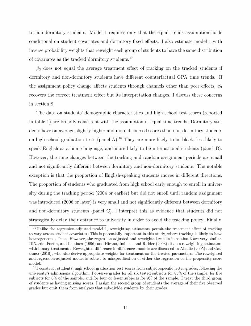
to non-dormitory students. Model 1 requires only that the equal trends assumption holds
conditional on student covariates and dormitory fixed effects. I also estimate model 1 with
inverse probability weights that reweight each group of students to have the same distribution
of covariates as the tracked dormitory students.17
β3 does not equal the average treatment effect of tracking on the tracked students if
dormitory and non-dormitory students have different counterfactual GPA time trends. If
the assignment policy change affects students through channels other than peer effects, β3
recovers the correct treatment effect but its interpretation changes. I discuss these concerns
in section 8.
The data on students’ demographic characteristics and high school test scores (reported
in table 1) are broadly consistent with the assumption of equal time trends. Dormitory stu-
dents have on average slightly higher and more dispersed scores than non-dormitory students
on high school graduation tests (panel A).18 They are more likely to be black, less likely to
speak English as a home language, and more likely to be international students (panel B).
However, the time changes between the tracking and random assignment periods are small
and not significantly different between dormitory and non-dormitory students. The notable
exception is that the proportion of English-speaking students moves in different directions.
The proportion of students who graduated from high school early enough to enroll in univer-
sity during the tracking period (2004 or earlier) but did not enroll until random assignment
was introduced (2006 or later) is very small and not significantly different between dormitory
and non-dormitory students (panel C). I interpret this as evidence that students did not
strategically delay their entrance to university in order to avoid the tracking policy. Finally,
17Unlike the regression-adjusted model 1, reweighting estimators permit the treatment effect of trackingto vary across student covariates. This is potentially important in this study, where tracking is likely to haveheterogeneous effects. However, the regression-adjusted and reweighted results in section 3 are very similar.DiNardo, Fortin, and Lemiuex (1996) and Hirano, Imbens, and Ridder (2003) discuss reweighting estimatorswith binary treatments. Reweighted difference-in-differences models are discussed in Abadie (2005) and Cat-taneo (2010), who also derive appropriate weights for treatment-on-the-treated parameters. The reweightedand regression-adjusted model is robust to misspecification of either the regression or the propensity scoremodel.
18I construct students’ high school graduation test scores from subject-specific letter grades, following theuniversity’s admissions algorithm. I observe grades for all six tested subjects for 85% of the sample, for fivesubjects for 6% of the sample, and for four or fewer subjects for 9% of the sample. I treat the third groupof students as having missing scores. I assign the second group of students the average of their five observedgrades but omit them from analyses that sub-divide students by their grades.
11

Table 1: Summary Statistics and Balance Tests
(1) (2) (3) (4) (5) (6)Entire Track Random Track Random Balancesample dorm dorm non-dorm non-dorm test p
Panel A: High school graduation test scoresMean score (standardized) 0.088 0.169 0.198 0.000 0.000 0.426A on graduation test 0.278 0.320 0.325 0.222 0.253 0.108≤C on graduation test 0.233 0.224 0.201 0.254 0.250 0.198
Panel B: Demographic characteristicsFemale 0.513 0.499 0.517 0.523 0.514 0.103Black 0.319 0.503 0.524 0.116 0.118 0.181White 0.423 0.354 0.332 0.520 0.495 0.851Other race 0.257 0.143 0.144 0.364 0.387 0.124English-speaking 0.714 0.593 0.560 0.851 0.863 0.001International 0.144 0.225 0.180 0.106 0.061 0.913
Panel C: Graduated high school in 2004 or earlier, necessary to enroll under trackingEligible for tracking 0.516 1.000 0.027 1.000 0.033 0.124Eligible | A student 0.475 1.000 0.002 1.000 0.010 0.037Eligible | ≤C student 0.527 1.000 0.039 1.000 0.050 0.330
Panel D: High school located in Cape Town, proxy for dormitory eligibilityCape Town high school 0.411 0.088 0.083 0.765 0.754 0.657Cape Town | A student 0.414 0.101 0.065 0.848 0.811 0.976Cape Town | ≤C student 0.523 0.146 0.186 0.798 0.800 0.224Notes: Table 1 reports summary statistics of student characteristics at the time of enrollment, for the entire sample (column1), tracked dormitory students (column 2), randomly assigned dormitory students (column 3), tracked non-dormitory students(column 4), and randomly assigned non-dormitory students (column 5). The p-values reported in column 6 are from testingwhether the mean change in each variable between the tracking and random assignment periods is equal for dormitory andnon-dormitory students.
there is a high and time-invariant correlation between living in a dormitory and graduat-
ing from a high school outside Cape Town. This relationship reflects the university’s policy
of restricting the number of students who live in Cape Town who may be admitted to the
dormitory system.19 The fact that this relationship does not change through time provides
some reassurance that students are not strategically choosing whether or not to live in dor-
mitories in response to the dormitory assignment policy change. This pattern may in part
reflect prospective students’ limited information about the dormitory assignment policy: the
19I do not observe students’ home addresses, which are used for the university’s dormitory admissions.Instead, I match records on students’ high schools to a public database of high school GIS codes. I thendetermine whether students attended high schools in or outside the Cape Town metropolitan area. This isan imperfect proxy of their home address for three reasons: long commutes and boarding schools are fairlycommon, the university allows students from very low-income neighborhoods on the outskirts of Cape Townto live in dormitories, and a small number of Cape Town students with medical conditions or exceptionalacademic records are permitted to live in the dormitories.
12

change was not announced in the university’s admissions materials or in internal, local, or
national media. On balance, these descriptive statistics support the identifying assumption
that dormitory and non-dormitory students’ mean GPAs would have experienced similar time
changes if the assignment policy had remained constant.20
The primary outcome variable is first-year students’ GPAs. The university did not at
this time report students’ GPAs or any other measure of average grades. I instead observe
students’ complete transcripts, which report percentage scores from 0 to 100 for each course.
I construct a credit-weighted average score and then transform this to have mean zero and
standard deviation one in the control group of non-dormitory students, separately by year.
The effects of tracking discussed below should therefore be interpreted in standard devia-
tions of GPA. The numerical scores are intended to be time-invariant measures of student
performance and are not typically “curved.”21 The nominal ceiling score of 100 does not
bind: the highest score any student obtains averaged across her courses is 97 and the 99th
percentile of student scores is 84. These features provide some reassurance that my results
are not driven by time-varying grading standards or by ceiling effects on the grades of top
students. I return to these potential concerns in section 8.
3 Effects of Tracking on Mean Outcomes
Tracked dormitory students obtain GPAs 0.13 standard deviations lower than randomly
assigned dormitory students (table 2 column 1). The 95% confidence interval is [-0.27, 0.01].
Controlling for dormitory fixed effects, student demographics, and high school graduation test
scores yields a slightly smaller treatment effect of -0.11 standard deviations with a narrower
95% confidence interval of [-0.17, -0.04] (column 2).22 The average effect of tracking is thus
20I also test the joint null hypothesis that the mean time changes in all the covariates are equal for dormitoryand non-dormitory students. The bootstrap p-value is 0.911.
21For example, mean percentage scores on Economics 1 and Mathematics 1 change by respectively six andnine points from year to year, roughly half of a standard deviation.
22The bootstrapped standard errors reported in table 2 allow clustering at the dormitory-year level. Non-dormitory students are treated as individual clusters, yielding 60 large clusters and approximately 7000singleton clusters. As a robustness check, I also use a wild cluster bootstrap (Cameron, Miller, and Gelbach,2008). The p-values are 0.090 for the basic regression model (column 1) and < 0.001 for the model withdormitory fixed effects and student covariates (column 3). I also account for the possibility of persistentdormitory-level shocks with a wild bootstrap clustered at the dormitory level. The p-values are 0.104 and0.002 for the models in columns 1 and 3.
13
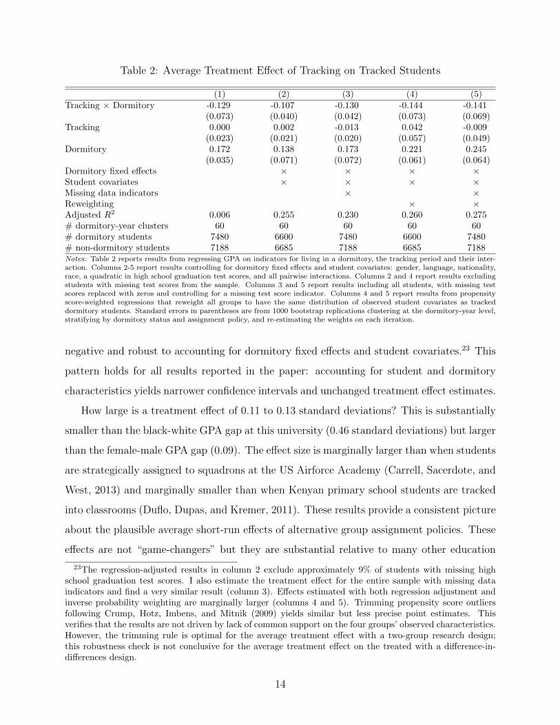
Table 2: Average Treatment Effect of Tracking on Tracked Students
(1) (2) (3) (4) (5)Tracking × Dormitory -0.129 -0.107 -0.130 -0.144 -0.141
(0.073) (0.040) (0.042) (0.073) (0.069)Tracking 0.000 0.002 -0.013 0.042 -0.009
(0.023) (0.021) (0.020) (0.057) (0.049)Dormitory 0.172 0.138 0.173 0.221 0.245
(0.035) (0.071) (0.072) (0.061) (0.064)Dormitory fixed effects × × × ×Student covariates × × × ×Missing data indicators × ×Reweighting × ×Adjusted R2 0.006 0.255 0.230 0.260 0.275# dormitory-year clusters 60 60 60 60 60# dormitory students 7480 6600 7480 6600 7480# non-dormitory students 7188 6685 7188 6685 7188Notes: Table 2 reports results from regressing GPA on indicators for living in a dormitory, the tracking period and their inter-action. Columns 2-5 report results controlling for dormitory fixed effects and student covariates: gender, language, nationality,race, a quadratic in high school graduation test scores, and all pairwise interactions. Columns 2 and 4 report results excludingstudents with missing test scores from the sample. Columns 3 and 5 report results including all students, with missing testscores replaced with zeros and controlling for a missing test score indicator. Columns 4 and 5 report results from propensityscore-weighted regressions that reweight all groups to have the same distribution of observed student covariates as trackeddormitory students. Standard errors in parentheses are from 1000 bootstrap replications clustering at the dormitory-year level,stratifying by dormitory status and assignment policy, and re-estimating the weights on each iteration.
negative and robust to accounting for dormitory fixed effects and student covariates.23 This
pattern holds for all results reported in the paper: accounting for student and dormitory
characteristics yields narrower confidence intervals and unchanged treatment effect estimates.
How large is a treatment effect of 0.11 to 0.13 standard deviations? This is substantially
smaller than the black-white GPA gap at this university (0.46 standard deviations) but larger
than the female-male GPA gap (0.09). The effect size is marginally larger than when students
are strategically assigned to squadrons at the US Airforce Academy (Carrell, Sacerdote, and
West, 2013) and marginally smaller than when Kenyan primary school students are tracked
into classrooms (Duflo, Dupas, and Kremer, 2011). These results provide a consistent picture
about the plausible average short-run effects of alternative group assignment policies. These
effects are not “game-changers” but they are substantial relative to many other education
23The regression-adjusted results in column 2 exclude approximately 9% of students with missing highschool graduation test scores. I also estimate the treatment effect for the entire sample with missing dataindicators and find a very similar result (column 3). Effects estimated with both regression adjustment andinverse probability weighting are marginally larger (columns 4 and 5). Trimming propensity score outliersfollowing Crump, Hotz, Imbens, and Mitnik (2009) yields similar but less precise point estimates. Thisverifies that the results are not driven by lack of common support on the four groups’ observed characteristics.However, the trimming rule is optimal for the average treatment effect with a two-group research design;this robustness check is not conclusive for the average treatment effect on the treated with a difference-in-differences design.
14
interventions.
Tracking changes peer groups in different ways: high-scoring students live with higher-
scoring peers and low-scoring students live with lower-scoring peers. The effects of tracking
are thus likely to vary systematically with students’ high school test scores. I explore this
heterogeneity in two ways. I first estimate conditional average treatment effects for different
subgroups of students. In section 4, I estimate quantile treatment effects of tracking, which
show how tracking changes the full distribution of GPAs.
I begin by estimating equation 1 fully interacted with an indicator for students who score
above the sample median on their high school graduation test. Above- and below-median
students’ GPAs fall respectively 0.01 and 0.24 standard deviations under tracking (cluster
bootstrap standard errors 0.06 and 0.07; p-value of difference 0.014). These very different
effects arise even though above- and below-median students experience “treatments” of sim-
ilar magnitude. Above- and below-median scoring students have residential peers who score
on average 0.20 standard deviations higher and 0.27 standard deviations lower under track-
ing. This is not consistent with a linear response to changes in mean peer quality.24 Either
low-scoring students are more sensitive to changes in their mean peer group composition or
GPA depends on some measure of peer quality other than mean test scores.
The near-zero treatment effect on above-median students is perhaps surprising. Splitting
the sample in two may be too coarse to discern positive effects on very high-scoring students.
I therefore estimate treatment effects throughout the distribution of high school test scores.
Figure 2 shows that tracking reduces GPA through more than half of the distribution. The
negative effects in the left tail are considerably larger than the positive effects in the right
tail, though they are not statistically different. I reject equality of the treatment effects and
changes in mean peer high school test scores in the right but not the left tail. These results
reinforce the finding that low-scoring students are substantially more sensitive to changes
in peer group composition than high-scoring students. Tracking may have a small positive
effect on students in the top quartile but this effect is imprecisely estimated.25
24I test whether the ratio of the treatment effect to the change in mean peer test scores is equal for above-and below-median students. The cluster bootstrap p-value is 0.070.
25A linear difference-in-differences model interacted with quartile or quintile indicators has positive butinsignificant point estimates in the top quartile or quintile.
15

Figure 2: Effects of Tracking on GPA by High School Test Scores
0 10 20 30 40 50 60 70 80 90 100
-0.8
-0.6
-0.4
-0.2
0
0.2
0.4
0.6
Percentiles of high school graduation test scores
Un
ive r
sity
GP
A /
Do
rmm
ate s
' me a
n te
s t s
core
s
Average treatment effect of tracking
Mean change in peers' HS test scores
Notes: Figure 2 is constructed by estimating a student-level local linear regression of GPA against high school graduation testscores. I estimate the regression separately for each of the four groups (tracking/randomization policy and dormitory/non-dormitory status). I evaluate the second difference at each percentile of the high school test score distribution. The dotted linesshow a 95% confidence interval constructed from a nonparametric percentile bootstrap clustering at the dormitory-year leveland stratifying by assignment policy and dormitory status. The dashed line shows the effect of tracking on mean peer groupcomposition, discussed in figure 1.
16

There is stronger evidence of heterogeneity across high school test scores than demo-
graphic subgroups. Treatment effects are larger on black than white students: -0.20 versus
-0.11 standard deviations. However, this difference is not significant (cluster bootstrap p-
value 0.488) and is almost zero after conditioning on high school test scores. I also estimate a
quadruple-differences model allowing the effect of tracking to differ across four race/academic
subgroups (black/white × above/below median). The point estimates show that tracking af-
fects below-median students more than above-median students within each race group and
affects black students more than white within each test score group. However, neither pattern
is significant at any conventional level. I thus lack the power to detect any heterogeneity by
race conditional on test scores. There is no evidence of gender heterogeneity: tracking lowers
female and male GPAs by 0.14 and 0.12 standard deviations respectively (cluster bootstrap
p-value 0.897). I conclude that high school test scores are the primary dimension of treatment
effect heterogeneity.
4 Effects of Tracking on the Distribution of Outcomes
I also estimate quantile treatment effects of tracking on the treated students, which show
how tracking changes the full GPA distribution. I first construct the counterfactual GPA
distribution that the tracked dormitory students would have obtained in the absence of track-
ing (figure 3, first panel). The horizontal distance between the observed and counterfactual
GPA distributions at each quantile equals the quantile treatment effect of tracking on the
treated students (figure 3, second panel). This provides substantially more information than
the average treatment effect but requires stronger identifying assumptions. Specifically, the
average effect is identified under the assumption that any time changes in the mean value of
unobserved GPA determinants are common across dormitory and non-dormitory students.
The quantile effects are identified under the assumption that there are no time changes in
the distribution of unobserved student-level GPA determinants for either dormitory or non-
dormitory students. GPA may experience time trends or cohort-level shocks provided these
are common across all students. I discuss the implementation of this model, developed by
Athey and Imbens (2006), in appendix A. I propose an extension to account flexibly for time
17

trends in observed student characteristics.
Figure 3 shows that tracking affects mainly the left tail. The point estimates are large and
negative in the first quintile (0.1 - 1.1 standard deviations), small and negative in the second
to fourth quintiles (≤ 0.2 standard deviations), and small and positive in the top quintile
(≤ 0.2 standard deviations). The estimates are relatively imprecise; the 95% confidence
interval excludes zero only in the first quintile.26 This reinforces the pattern that the negative
average effect of tracking is driven by large negative effects on the left tail of the GPA or
high school test score distribution.
There is no necessary relationship between figures 2 and 3. Figure 2 shows that the
average treatment effect of tracking is large and negative for students with low high school
graduation test scores. Figure 3 shows that the quantile treatment effect of tracking is large
and negative on the left tail of the GPA distribution. The quantile results capture treatment
effect heterogeneity between and within groups of students with similar high school test
scores. However, they do not recover treatment effects on specific students or groups of
students without additional assumptions. See Bitler, Gelbach, and Hoynes (2010) for further
discussion on this relationship.27
5 Effects of Tracking on Inequality of Outcomes
The counterfactual GPA distribution estimated above also provides information about the
relationship between tracking and academic inequality. Specifically, I calculate several stan-
dard inequality measures on the observed and counterfactual distributions. The differences
between these measures are the inequality treatment effects of tracking on the tracked stu-
dents.28 The literature on academic tracking emphasizes inequality concerns (Betts, 2011).
26I construct the 95% confidence interval at each half-percentile using a percentile cluster bootstrap. Thevalidity of the bootstrap has not been formally established for the nonlinear difference-in-differences model.However, Athey and Imbens (2006) report that bootstrap confidence intervals have better coverage rates in asimulation study than confidence intervals based on plug-in estimators of the asymptotic covariance matrix.
27Garlick (2012) presents an alternative approach to rank-based distributional analysis. Using this ap-proach, I estimate the effect of tracking on the probability that students change their rank in the distributionof academic outcomes from high school to the first year of university. I find no effect on several measuresof rank changes. Informally, this shows that random dormitory assignment, relative to tracking, helps low-scoring students to “catch-up” to their high-scoring peers but does not facilitate “overtaking.”
28I apply the same principle to calculate mean GPA for the counterfactual distribution. The observedmean is 0.16 standard deviations lower than the counterfactual mean (cluster bootstrap standard error 0.07).
18

Figure 3: Quantile Treatment Effects of Tracking on the Tracked Students
-4 -3 -2 -1 0 1 2 30
20
40
60
80
100
University GPA
Per
cen
tile s
Observeddistribution
Counterfactualdistribution
0 10 20 30 40 50 60 70 80 90 100
-1.6
-1.4
-1.2
-1
-0.8
-0.6
-0.4
-0.2
0
0.2
0.4
0.6
Percentiles of university GPA
Un
ive r
sity
GP
A
Quantile treatment effects of tracking
Notes: The first panel shows the observed GPA distribution for tracked dormitory students (solid line) and the counterfactualconstructed using the reweighted nonlinear difference-in-differences model discussed in appendix A (dashed line). The propensityscore weights are constructed from a model including student gender, language, nationality, race, a quadratic in high schoolgraduation test scores, all pairwise interactions, and dormitory fixed effects. The second panel shows the horizontal distancebetween the observed and counterfactual GPA distributions evaluated at each half-percentile. The axes are reversed for easeof interpretation. The dotted lines show a 95% confidence interval constructed from a percentile bootstrap clustering at thedormitory-year level, stratifying by assignment policy and dormitory status, and re-estimating the weights on each iteration.
19
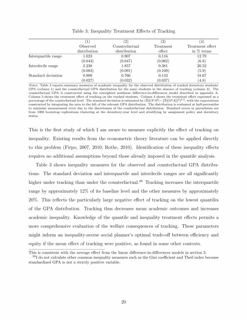
Table 3: Inequality Treatment Effects of Tracking
(1) (2) (3) (4)Observed Counterfactual Treatment Treatment effect
distribution distribution effect in % termsInterquartile range 1.023 0.907 0.116 12.79
(0.043) (0.047) (0.062) (6.8)Interdecile range 2.238 1.857 0.381 20.52
(0.083) (0.091) (0.109) (5.9)Standard deviation 0.909 0.766 0.143 18.67
(0.027) (0.032) (0.037) (4.8)Notes: Table 3 reports summary measures of academic inequality for the observed distribution of tracked dormitory students’GPA (column 1) and the counterfactual GPA distribution for the same students in the absence of tracking (column 2). Thecounterfactual GPA is constructed using the reweighted nonlinear difference-in-differences model described in appendix A.Column 3 shows the treatment effect of tracking on the tracked students. Column 4 shows the treatment effect expressed as apercentage of the counterfactual level. The standard deviation is estimated by (E[GPA2]−{E[GPA]}2)0.5, with the expectationsconstructed by integrating the area to the left of the relevant GPA distribution. The distribution is evaluated at half-percentilesto minimize measurement error due to the discreteness of the counterfactual distribution. Standard errors in parentheses arefrom 1000 bootstrap replications clustering at the dormitory-year level and stratifying by assignment policy and dormitorystatus.
This is the first study of which I am aware to measure explicitly the effect of tracking on
inequality. Existing results from the econometric theory literature can be applied directly
to this problem (Firpo, 2007, 2010; Rothe, 2010). Identification of these inequality effects
requires no additional assumptions beyond those already imposed in the quantile analysis.
Table 3 shows inequality measures for the observed and counterfactual GPA distribu-
tions. The standard deviation and interquartile and interdecile ranges are all significantly
higher under tracking than under the counterfactual.29 Tracking increases the interquartile
range by approximately 12% of its baseline level and the other measures by approximately
20%. This reflects the particularly large negative effect of tracking on the lowest quantiles
of the GPA distribution. Tracking thus decreases mean academic outcomes and increases
academic inequality. Knowledge of the quantile and inequality treatment effects permits a
more comprehensive evaluation of the welfare consequences of tracking. These parameters
might inform an inequality-averse social planner’s optimal trade-off between efficiency and
equity if the mean effect of tracking were positive, as found in some other contexts.
This is consistent with the average effect from the linear difference-in-differences models in section 3.29I do not calculate other common inequality measures such as the Gini coefficient and Theil index because
standardized GPA is not a strictly positive variable.
20
6 Effects of Random Variation in Dormitory Composi-
tion
The principal research design uses cross-policy variation by comparing tracked and randomly
assigned dormitory students. My second research design uses cross-dormitory variation in
peer group composition induced by random assignment. I first use a standard test to confirm
the presence of residential peer effects, providing additional evidence that the main results
are not driven by confounding factors. I document differences in dormitory-level peer effects
within and between demographic and academic subgroups, providing some information about
mechanisms. In section 7, I explore whether peer effects estimated using random dormitory
assignment can predict the distributional effects of tracking. I find that low-scoring students
are more sensitive to changes in peer group composition than high-scoring students, which
is qualitatively consistent with the effect of tracking. Quantitative predictions are, however,
sensitive to model specification choices.
I first estimate the standard linear-in-means model (Manski, 1993):
GPAid = α0 + α1HSid + α2HSd + ~α ~Xid + ~µd + εid, (2)
where HSid and HSd are individual and mean dormitory high school graduation test scores,
~Xid is a vector of student demographic characteristics, and ~µ is a vector of dormitory fixed
effects. α2 measures the average gain in GPA from a one standard deviation increase in
the mean high school graduation test scores of one’s residential peers.30 Random dormitory
assignment ensures that HSd is uncorrelated with individual students’ unobserved charac-
teristics so α2 can be consistently estimated by least squares.31 However, random assignment
also means that average high school graduation test scores are equal in expectation. α2
is identified using sample variation in scores across dormitories due to finite numbers of
30α2 captures both “endogenous” effects of peers’ GPA and “exogenous” effects of peers’ high schoolgraduation test scores, using Manski’s terminology. Following the bulk of the peer effects literature, I do notattempt to separate these effects.
31The observed dormitory assignments are consistent with randomization. I fail to reject equality ofdormitory means for high school graduation test scores (bootstrap p-value 0.762), proportion black (0.857),proportion white (0.917), proportion other races (0.963), proportion English-speaking (0.895), proportioninternational (0.812), and for all covariates jointly (0.886).
21
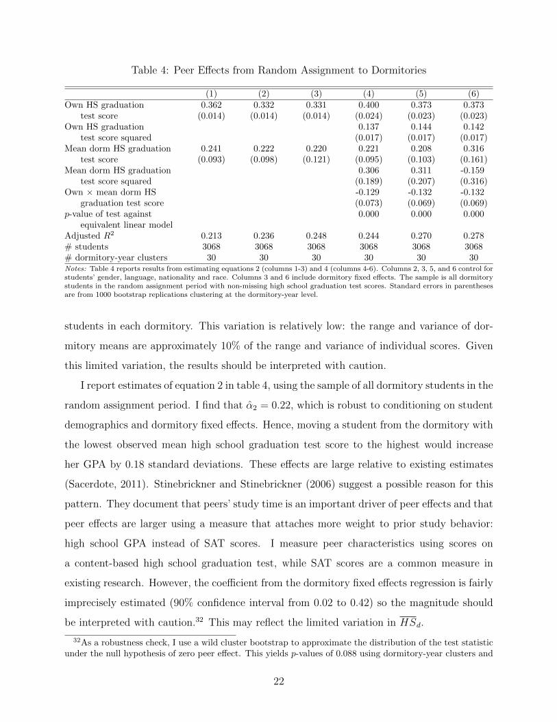
Table 4: Peer Effects from Random Assignment to Dormitories
(1) (2) (3) (4) (5) (6)Own HS graduation 0.362 0.332 0.331 0.400 0.373 0.373
test score (0.014) (0.014) (0.014) (0.024) (0.023) (0.023)Own HS graduation 0.137 0.144 0.142
test score squared (0.017) (0.017) (0.017)Mean dorm HS graduation 0.241 0.222 0.220 0.221 0.208 0.316
test score (0.093) (0.098) (0.121) (0.095) (0.103) (0.161)Mean dorm HS graduation 0.306 0.311 -0.159
test score squared (0.189) (0.207) (0.316)Own × mean dorm HS -0.129 -0.132 -0.132
graduation test score (0.073) (0.069) (0.069)p-value of test against 0.000 0.000 0.000
equivalent linear modelAdjusted R2 0.213 0.236 0.248 0.244 0.270 0.278# students 3068 3068 3068 3068 3068 3068# dormitory-year clusters 30 30 30 30 30 30Notes: Table 4 reports results from estimating equations 2 (columns 1-3) and 4 (columns 4-6). Columns 2, 3, 5, and 6 control forstudents’ gender, language, nationality and race. Columns 3 and 6 include dormitory fixed effects. The sample is all dormitorystudents in the random assignment period with non-missing high school graduation test scores. Standard errors in parenthesesare from 1000 bootstrap replications clustering at the dormitory-year level.
students in each dormitory. This variation is relatively low: the range and variance of dor-
mitory means are approximately 10% of the range and variance of individual scores. Given
this limited variation, the results should be interpreted with caution.
I report estimates of equation 2 in table 4, using the sample of all dormitory students in the
random assignment period. I find that α2 = 0.22, which is robust to conditioning on student
demographics and dormitory fixed effects. Hence, moving a student from the dormitory with
the lowest observed mean high school graduation test score to the highest would increase
her GPA by 0.18 standard deviations. These effects are large relative to existing estimates
(Sacerdote, 2011). Stinebrickner and Stinebrickner (2006) suggest a possible reason for this
pattern. They document that peers’ study time is an important driver of peer effects and that
peer effects are larger using a measure that attaches more weight to prior study behavior:
high school GPA instead of SAT scores. I measure peer characteristics using scores on
a content-based high school graduation test, while SAT scores are a common measure in
existing research. However, the coefficient from the dormitory fixed effects regression is fairly
imprecisely estimated (90% confidence interval from 0.02 to 0.42) so the magnitude should
be interpreted with caution.32 This may reflect the limited variation in HSd.
32As a robustness check, I use a wild cluster bootstrap to approximate the distribution of the test statisticunder the null hypothesis of zero peer effect. This yields p-values of 0.088 using dormitory-year clusters and
22
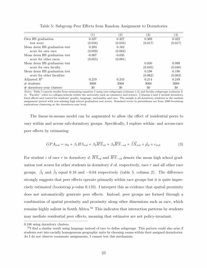
Table 5: Subgroup Peer Effects from Random Assignment to Dormitories
(1) (2) (3) (4)Own HS graduation 0.327 0.327 0.369 0.322
test score (0.016) (0.016) (0.017) (0.017)Mean dorm HS graduation test 0.203 0.162
score for own race (0.059) (0.083)Mean dorm HS graduation test -0.007 -0.035
score for other races (0.055) (0.091)Mean dorm HS graduation test 0.050 0.099
score for own faculty (0.045) (0.048)Mean dorm HS graduation test 0.198 0.190
score for other faculties (0.062) (0.083)Adjusted R2 0.219 0.243 0.214 0.249# students 3068 3068 3068 3068# dormitory-year clusters 30 30 30 30Notes: Table 5 reports results from estimating equation 3 using race subgroups (columns 1-2) and faculty subgroups (columns 3-4). “Faculty” refers to colleges/schools within the university such as commerce and science. Columns 2 and 4 include dormitoryfixed effects and control for students’ gender, language, nationality and race. The sample is all dormitory students in the randomassignment period with non-missing high school graduation test scores. Standard errors in parentheses are from 1000 bootstrapreplications clustering at the dormitory-year level.
The linear-in-means model can be augmented to allow the effect of residential peers to
vary within and across sub-dormitory groups. Specifically, I explore within- and across-race
peer effects by estimating:
GPAird = α0 + β1HSird + β2HSrd + β3HS−rd + ~β ~Xird + ~µd + εird. (3)
For student i of race r in dormitory d, HSrd and HS−rd denote the mean high school grad-
uation test scores for other students in dormitory d of, respectively, race r and all other race
groups. β2 and β3 equal 0.16 and −0.04 respectively (table 5, column 2). The difference
strongly suggests that peer effects operate primarily within race groups but it is quite impre-
cisely estimated (bootstrap p-value 0.110). I interpret this as evidence that spatial proximity
does not automatically generate peer effects. Instead, peer groups are formed through a
combination of spatial proximity and proximity along other dimensions such as race, which
remains highly salient in South Africa.33 This indicates that interaction patterns by students
may mediate residential peer effects, meaning that estimates are not policy-invariant.
0.186 using dormitory clusters.33I find a similar result using language instead of race to define subgroups. This pattern could also arise if
students sort into racially homogeneous geographic units by choosing rooms within their assigned dormitories.As I do not observe roommate assignments, I cannot test this mechanism.
23

I also explore the content of the interaction patterns that generate residential peer ef-
fects by estimating equation 3 using faculty/school/college groups instead of race groups.
The estimated within- and across-faculty peer effects are respectively 0.10 and 0.19 (cluster
bootstrap standard errors 0.05 and 0.08). Despite their relative imprecision, these results
suggests that within-faculty peer effects are not systematically stronger than cross-faculty
peer effects.34 This result is not consistent with peer effects being driven by direct aca-
demic collaboration such as joint work on problem sets or joint studying for examinations.
Interviews with students at the university suggest two channels through which peer effects
operate: time allocation over study and leisure activities, and transfers of tacit knowledge
such as study skills, norms about how to interact with faculty, and strategies for navigating
academic bureaucracy. This is consistent with prior findings of strong peer effects on study
time (Stinebrickner and Stinebrickner, 2006) and social activities (Duncan, Boisjoly, Kremer,
Levy, and Eccles, 2005).
Combining the race- and faculty-level peer effects results indicates that spatial proximity
alone does not generate peer effects. Some direct interaction is also necessary and is more
likely when students are also socially proximate. However, the relevant form of the interaction
is not direct academic collaboration. The research design and data cannot conclusively
determine what interactions do generate the estimated peer effects.
34Each student at the University of Cape Town is registered in one of six faculties: commerce, engineering,health sciences, humanities and social sciences, law, and science. Some students take courses exclusivelywithin their faculty (engineering, health sciences) while some courses overlap across multiple faculties (in-troductory statistics is offered in commerce and science, for example). I obtain similar results using course-specific grades as the outcome and allowing residential peer effects to differ at the course level. For example,I estimate equations 2 and 3 with Introductory Microeconomics grades as an outcome. I find that thereare strong peer effects on grades in this course (α2 = 0.34 with cluster bootstrap standard error 0.15) but
they are not driven primarily by other students in the same course (β2 = 0.06 and β3 = 0.17 with clusterbootstrap standard errors 0.17 and 0.15). This, and other course-level regressions, are consistent with themain results but the smaller sample sizes yield relatively imprecise estimates that are somewhat sensitive tothe inclusion of covariates.
24
7 Reconciling Cross-Policy and Cross-Dormitory Re-
sults
The linear-in-means model restricts average GPA to be invariant to any group reassignment:
moving a strong student to a new group has equal but oppositely signed effects on her old
and new peers’ average GPA. If the true GPA production function is linear, then the average
treatment effect of tracking relative to random assignment must be zero. I therefore estimate
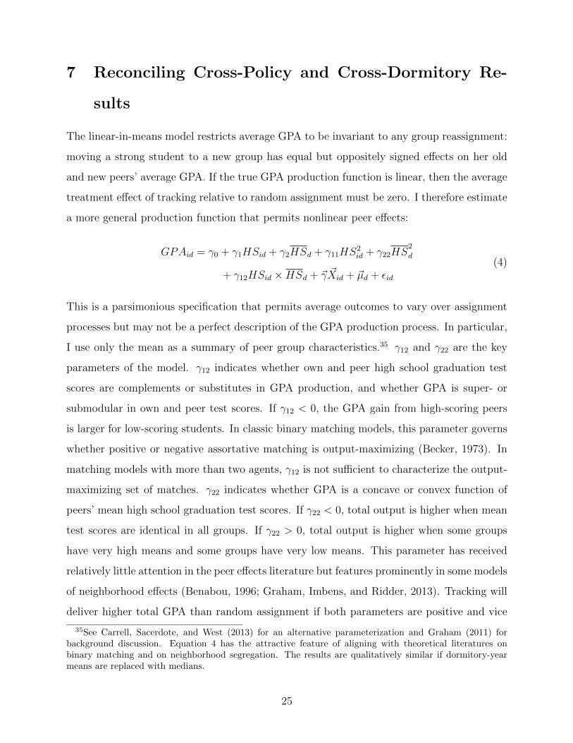
a more general production function that permits nonlinear peer effects:
GPAid = γ0 + γ1HSid + γ2HSd + γ11HS2id + γ22HS
2
d
+ γ12HSid ×HSd + ~γ ~Xid + ~µd + εid
(4)
This is a parsimonious specification that permits average outcomes to vary over assignment
processes but may not be a perfect description of the GPA production process. In particular,
I use only the mean as a summary of peer group characteristics.35 γ12 and γ22 are the key
parameters of the model. γ12 indicates whether own and peer high school graduation test
scores are complements or substitutes in GPA production, and whether GPA is super- or
submodular in own and peer test scores. If γ12 < 0, the GPA gain from high-scoring peers
is larger for low-scoring students. In classic binary matching models, this parameter governs
whether positive or negative assortative matching is output-maximizing (Becker, 1973). In
matching models with more than two agents, γ12 is not sufficient to characterize the output-
maximizing set of matches. γ22 indicates whether GPA is a concave or convex function of
peers’ mean high school graduation test scores. If γ22 < 0, total output is higher when mean
test scores are identical in all groups. If γ22 > 0, total output is higher when some groups
have very high means and some groups have very low means. This parameter has received
relatively little attention in the peer effects literature but features prominently in some models
of neighborhood effects (Benabou, 1996; Graham, Imbens, and Ridder, 2013). Tracking will
deliver higher total GPA than random assignment if both parameters are positive and vice
35See Carrell, Sacerdote, and West (2013) for an alternative parameterization and Graham (2011) forbackground discussion. Equation 4 has the attractive feature of aligning with theoretical literatures onbinary matching and on neighborhood segregation. The results are qualitatively similar if dormitory-yearmeans are replaced with medians.
25

versa. If the parameters have different signs, the average effect of tracking is ambiguous.36
Estimates from equation 4 are shown in table 4 columns 4, 5 (controlling for student
demographics) and 6 (with dormitory fixed effects). γ12 is negative and marginally statis-
tically significant across all specifications. The point estimate of −0.13 (cluster bootstrap
standard error 0.07) implies the GPA gain from an increase in peers’ mean test scores is 0.2
standard deviations larger for students at the 25th percentile of the high school test score
distribution than students at the 75th percentile. This is consistent with the section 4 result
that low-scoring students are hurt more by tracking than high-scoring students are helped.
However, the sign of γ22 flips from positive to negative with the inclusion of dormitory fixed
effects. It is thus unclear whether GPA is concave or convex in mean peer group test scores.
I draw three conclusions from these results. First, there is clear evidence of nonlinear peer
effects from the cross-dormitory variation generated under random assignment. Likelihood
ratio tests prefer the nonlinear models in columns 4-6 to the corresponding linear models in
columns 1-3. Second, peer effects estimates using randomly induced cross-dormitory variation
may be sensitive to the support of the data. Using dormitory fixed effects reduces the variance
of HSd from 0.19 to 0.11. This leads to different conclusions about the curvature of the GPA
production function in columns 5 and 6. Third, the results from the fixed effects specification
(column 6) are qualitatively consistent with the negative average treatment effect of tracking.
Are the coefficient estimates from equation 4 quantitatively, as well as qualitatively, con-
sistent with the observed treatment effects of tracking? I combine coefficients from estimating
equation 4 for randomly assigned dormitory students with observed values of individual- and
dormitory-level regressors for tracked dormitory students. I then predict the level of GPA
and the treatment effect of tracking for students in the first and fourth quartiles of the high
school graduation test score distribution. I compare these predictions to observed GPA for
tracked dormitory students and to the difference-in-differences treatment effect of tracking.
The results in table 6 show that the predictions are sensitive to specification of equation
36To derive this result, note that E[HSd|HSid] = HSid under tracking and E[HSid] under random as-
signment. Hence, E[HSidHSd] and E[HS2
d] both equal E[HS2id] under tracking and E[HSid]2 under ran-
dom assignment. Plugging these results into equation 4 for each assignment policy yields E[Yid|Tracking]−E[Yid|Randomization] = σ2
HS (γ22 + γ12). This simple demonstration assumes an infinite number of studentsand dormitories. This assumption is not necessary but simplifies the exposition.
26
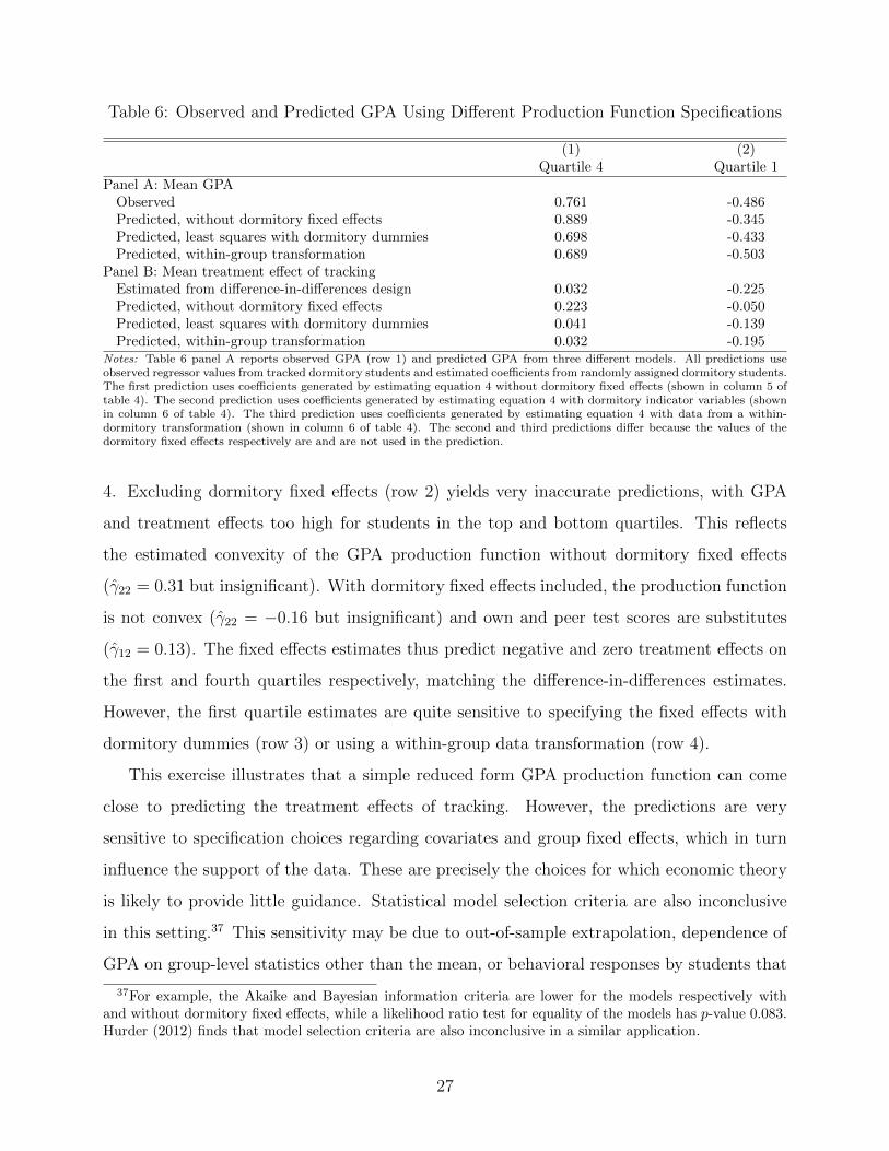
Table 6: Observed and Predicted GPA Using Different Production Function Specifications
(1) (2)Quartile 4 Quartile 1
Panel A: Mean GPAObserved 0.761 -0.486Predicted, without dormitory fixed effects 0.889 -0.345Predicted, least squares with dormitory dummies 0.698 -0.433Predicted, within-group transformation 0.689 -0.503
Panel B: Mean treatment effect of trackingEstimated from difference-in-differences design 0.032 -0.225Predicted, without dormitory fixed effects 0.223 -0.050Predicted, least squares with dormitory dummies 0.041 -0.139Predicted, within-group transformation 0.032 -0.195
Notes: Table 6 panel A reports observed GPA (row 1) and predicted GPA from three different models. All predictions useobserved regressor values from tracked dormitory students and estimated coefficients from randomly assigned dormitory students.The first prediction uses coefficients generated by estimating equation 4 without dormitory fixed effects (shown in column 5 oftable 4). The second prediction uses coefficients generated by estimating equation 4 with dormitory indicator variables (shownin column 6 of table 4). The third prediction uses coefficients generated by estimating equation 4 with data from a within-dormitory transformation (shown in column 6 of table 4). The second and third predictions differ because the values of thedormitory fixed effects respectively are and are not used in the prediction.
4. Excluding dormitory fixed effects (row 2) yields very inaccurate predictions, with GPA
and treatment effects too high for students in the top and bottom quartiles. This reflects
the estimated convexity of the GPA production function without dormitory fixed effects
(γ22 = 0.31 but insignificant). With dormitory fixed effects included, the production function
is not convex (γ22 = −0.16 but insignificant) and own and peer test scores are substitutes
(γ12 = 0.13). The fixed effects estimates thus predict negative and zero treatment effects on
the first and fourth quartiles respectively, matching the difference-in-differences estimates.
However, the first quartile estimates are quite sensitive to specifying the fixed effects with
dormitory dummies (row 3) or using a within-group data transformation (row 4).
This exercise illustrates that a simple reduced form GPA production function can come
close to predicting the treatment effects of tracking. However, the predictions are very
sensitive to specification choices regarding covariates and group fixed effects, which in turn
influence the support of the data. These are precisely the choices for which economic theory
is likely to provide little guidance. Statistical model selection criteria are also inconclusive
in this setting.37 This sensitivity may be due to out-of-sample extrapolation, dependence of
GPA on group-level statistics other than the mean, or behavioral responses by students that
37For example, the Akaike and Bayesian information criteria are lower for the models respectively withand without dormitory fixed effects, while a likelihood ratio test for equality of the models has p-value 0.083.Hurder (2012) finds that model selection criteria are also inconclusive in a similar application.
27
make peer effects policy-sensitive.
8 Alternative Explanations for the Effects of Tracking
I consider four alternative explanations that might have generated the observed GPA differ-
ence between tracked and randomly assigned dormitory students. The first two explanations
are violations of the “parallel time changes” assumption: time-varying student selection re-
garding whether or not to live in a dormitory and differential time trends in dormitory and
non-dormitory students’ characteristics. The third explanation is that the treatment effects
are an artefact of the grading system and do not reflect any real effect on learning. The
fourth explanation is that dormitory assignment affects GPA through a mechanism other
than peer effects; this would not invalidate the results but would change their interpretation.
8.1 Selection into Dormitory Status
The research design assumes that non-dormitory students are an appropriate control group for
any time trends or cohort effects on dormitory students’ outcomes. This assumption may fail
if students select whether or not to live in a dormitory based on the assignment policy. I argue
that such behavior is unlikely and that my results are robust to accounting for selection. First,
the change in dormitory assignment policy was not officially announced or widely publicized,
limiting students’ ability to respond. Second, table 1 shows that there are approximately
equal time changes in dormitory and non-dormitory students’ demographic characteristics
and high school graduation test scores. Third, the results are robust to accounting for small
differences in these time changes using regression or reweighting.
Fourth, admission rules cap the number of students from Cape Town who may be admit-
ted to the dormitory system. Given this rule, I use an indicator for whether each student
attended a high school outside Cape Town as an instrument for whether the student lives in
a dormitory. High school location is an imperfect proxy for home address, which I do not
observe. Nonetheless, the instrument strongly predicts dormitory status: 76% of non-Cape
Town students and 8% of Cape Town students live in dormitories. The intention-to-treat and
instrumented treatment effects (table 7, columns 2 and 3) are very similar to the treatment
28

effects without instruments (table 2).
8.2 Differential Time Trends in Student Characteristics
The research design assumes that dormitory and non-dormitory students’ GPAs do not have
different time trends for reasons unrelated to the change in assignment policy. I present
three arguments against this concern. First, I extend the analysis to include data from the
2001–2002 academic years (“early tracking”), in addition to 2004–2005 (“late tracking”) and
2007–2008 (random assignment). I do not observe dormitory assignments in 2001–2002 so I
report only intention-to-treat effects.38 The raw data are shown in the first panel of figure
4. I estimate the effect of tracking under several possible violations of the parallel trends
assumption. The average effect of tracking comparing 2001-2005 to 2007-2008 is -0.09 with
standard error 0.04 (table 7, column 4). This estimate is appropriate if one group of students
experiences a transitory shock in 2004/2005. A placebo test comparing the difference between
Cape Town and non-Cape Town students’ GPAs in 2001-2002 and 2004-2005 yields a small
positive but insignificant effect of 0.06 (standard error 0.05). I subtract the placebo test
result from the original treatment effect estimate to obtain a “trend-adjusted” treatment
effect of -0.18 with standard error 0.10 (table 7, column 6). This estimate is appropriate
if the two groups of students have linear but non-parallel time trends and are subject to
common transitory shocks (Heckman and Hotz, 1989). Finally, I estimate a linear time trend
in the GPA gap between Cape Town and non-Cape Town students from 2001 to 2005. I
then project that trend into 2007–2008 and estimate the deviation of the GPA gap from
its predicted level. This method yields a treatment effect of random assignment relative to
tracking of 0.14 with standard error 0.09 (table 7, column 5). This estimate is appropriate
if the two groups of students have non-parallel time trends whose difference is linear. The
effect of tracking is relatively robust across the standard difference-in-differences model and
all three models estimated under weaker assumptions. However, there is some within-policy
38The cluster bootstrap standard errors do not take into account potential clustering within (unobserved)dormitories in 2001–2002 and so may be downward-biased. I omit the 2003 academic year because the dataextract I received from the university had missing identifiers for approximately 80% of students in that year.I omit 2006 because first year students were randomly assigned to dormitories that still contained trackedsecond year students. The results are robust to including 2006.
29
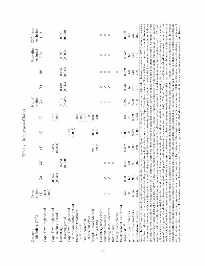
Tab
le7:
Rob
ust
nes
sC
hec
ks
Ou
tcom
eD
orm
No.
of
%cr
edit
sG
PA|n
on
-(d
efau
ltis
GP
A)
stu
den
tcr
edit
sex
clu
ded
excl
usi
on
(1)
(2)
(3)
(4)
(5)
(6)
(7)
(8)
(9)
(10)
(11)
Cap
eT
own
hig
hsc
hool
0.60
1(0
.019
)C
ape
Tow
nh
igh
sch
ool
-0.0
93-0
.090
-0.1
15
×tr
ackin
gp
erio
d(0
.034
)(0
.044)
(0.0
55)
Dor
mit
ory×
-0.1
33
-0.0
13
-0.1
39
-0.1
65
0.0
27
-0.0
77
trac
kin
gp
erio
d(0
.050)
(0.0
38)
(0.0
43)
(0.0
44)
(0.0
05)
(0.0
50)
Cap
eT
own
hig
hsc
hool
0.1
41
×ra
nd
omiz
atio
np
erio
d(0
.093)
Pla
ceb
op
re-t
reat
men
t0.0
58
diff
-in
-diff
(0.0
52)
Tre
nd
-cor
rect
ed-0
.175
trea
tmen
teff
ect
(0.1
00)
Sam
ple
per
iod
(def
ault
2001-
2001-
2001-
is20
04-2
008)
-2008
-2008
-2008
Dor
mit
ory
fixed
effec
ts×
××
××
Stu
den
tco
vari
ates
××
××
××
××
Mis
sin
gd
ata
ind
icat
ors
××
××
××
××
Inst
rum
ents
×F
acu
lty
fixed
effec
ts×
Pre
-tre
atm
ent
tim
etr
end
×A
dju
sted
R2
0.52
50.
231
0.2
31
0.0
02
0.0
00
0.0
00
0.1
27
0.2
42
0.2
29
0.0
52
0.3
02
#d
orm
-yea
rcl
ust
ers
6060
60
60
60
60
60
52
60
60
60
#d
orm
itor
yst
ud
ents
6915
6915
6915
8509
8509
8509
7480
6795
7480
7480
7449
#n
on-d
orm
stu
den
ts64
6664
666466
14203
14203
14203
7188
7188
7188
7188
7043
Notes:
Tab
le7
rep
ort
sre
sult
sfr
om
the
rob
ust
nes
sch
ecks
dis
cuss
edin
sub
sect
ion
s8.1
-8.3
.C
olu
mn
s1–3
show
the
rela
tion
ship
bet
wee
nst
ud
ents
’G
PA
(ou
tcom
e),
wh
eth
erth
eylive
ind
orm
itori
es(t
reatm
ent)
an
dw
het
her
they
gra
du
ate
dfr
om
hig
hsc
hools
loca
ted
ou
tsid
eC
ap
eT
ow
n(i
nst
rum
ent)
.T
he
coeffi
cien
tof
inte
rest
ison
the
trea
tmen
tor
inst
rum
ent
inte
ract
edw
ith
an
ind
icato
rfo
rw
het
her
stu
den
tsatt
end
edth
eu
niv
ersi
tyd
uri
ng
the
track
ing
per
iod
.C
olu
mn
1sh
ow
sth
efi
rst
stage
esti
mate
,co
lum
n2
show
sth
ere
du
ced
form
esti
mate
,an
dco
lum
nsh
ow
sth
eIV
esti
mate
.D
orm
itory
fixed
effec
tsare
excl
ud
edb
ecau
seth
eyare
colin
ear
wit
hth
efi
rst
stage
ou
tcom
e.C
olu
mn
s4–6
use
data
from
2001-2
002,
2004-2
005,
an
d2007-2
008
tote
stth
ep
ara
llel
tim
etr
end
sass
um
pti
on
.C
olu
mn
4re
port
sa
diff
eren
ce-i
n-d
iffer
ence
ses
tim
ate
com
pari
ng
all
fou
rob
serv
edyea
rsof
track
ing
toth
etw
oob
serv
edyea
rsof
ran
dom
ass
ign
men
t.C
olu
mn
5re
port
sth
ed
iffer
ence
bet
wee
nob
serv
edG
PA
un
der
ran
dom
ass
ign
men
tan
dp
red
icte
dG
PA
from
alin
ear
tim
etr
end
extr
ap
ola
ted
from
the
track
ing
per
iod
.C
olu
mn
6re
port
sth
ep
lace
bo
diff
eren
ce-i
n-d
iffer
ence
ste
stco
mp
ari
ng
the
firs
ttw
oyea
rsof
track
ing
toth
ela
sttw
oyea
rsof
track
ing
an
dth
ed
iffer
ence
bet
wee
nth
em
ain
an
dp
lace
bo
effec
tsfo
llow
ing
Hec
km
an
an
dH
otz
(1989).
Colu
mn
7re
port
sa
diff
eren
ce-i
n-d
iffer
ence
ses
tim
ate
wit
hth
ecr
edit
-wei
ghte
dnu
mb
erof
cou
rses
as
the
ou
tcom
e.C
olu
mn
8re
port
sa
diff
eren
ce-i
n-d
iffer
ence
ses
tim
ate
excl
ud
ing
dorm
itori
esth
at
are
eith
erob
serv
edin
on
lyon
ep
erio
dor
use
ad
iffer
ent
ad
mis
sion
rule
.C
olu
mn
9re
port
sa
diff
eren
ce-i
n-d
iffer
ence
ses
tim
ate
incl
ud
ing
colleg
e/fa
cult
y/sc
hool
fixed
effec
ts.
Colu
mn
10
rep
ort
sa
diff
eren
ce-i
n-d
iffer
ence
ses
tim
ate
wit
hth
ecr
edit
-wei
ghte
dp
erce
nta
ge
of
cou
rses
from
wh
ich
stu
den
tsare
aca
dem
icall
yex
clu
ded
as
the
ou
tcom
e.C
olu
mn
11
rep
ort
sa
diff
eren
ce-i
n-d
iffer
ence
ses
tim
ate
wit
hG
PA
calc
ula
ted
usi
ng
on
lygra
des
from
non
-excl
ud
edco
urs
esas
the
ou
tcom
e.S
tan
dard
erro
rsin
pare
nth
eses
are
from
1000
boots
trap
rep
lica
tion
s,st
rati
fyin
gby
ass
ign
men
tp
oli
cyan
dd
orm
itory
statu
s.T
he
boots
trap
resa
mp
les
dorm
itory
-yea
rcl
ust
ers
exce
pt
for
the
2001-2
002
data
inco
lum
ns
4-6
,fo
rw
hic
hd
orm
itory
ass
ign
men
tsare
not
ob
serv
ed.
30
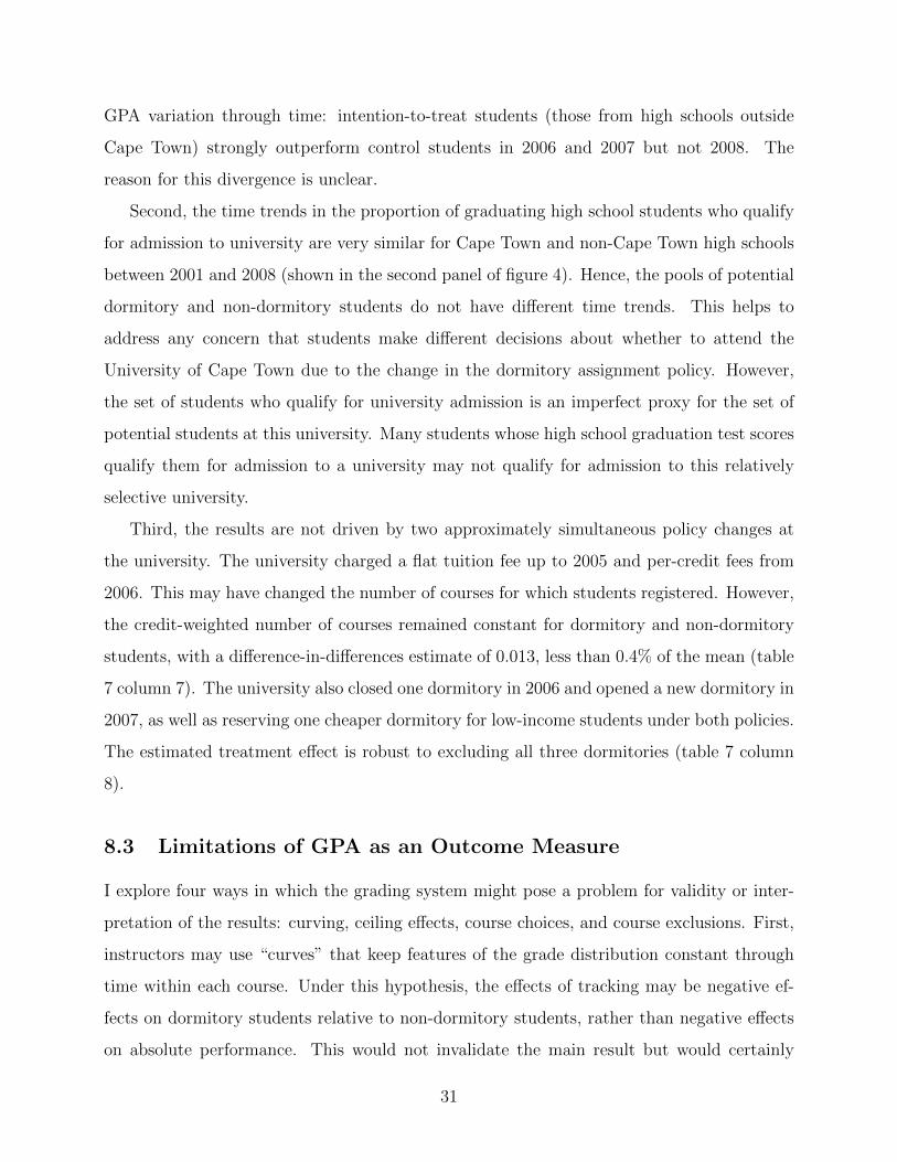
GPA variation through time: intention-to-treat students (those from high schools outside
Cape Town) strongly outperform control students in 2006 and 2007 but not 2008. The
reason for this divergence is unclear.
Second, the time trends in the proportion of graduating high school students who qualify
for admission to university are very similar for Cape Town and non-Cape Town high schools
between 2001 and 2008 (shown in the second panel of figure 4). Hence, the pools of potential
dormitory and non-dormitory students do not have different time trends. This helps to
address any concern that students make different decisions about whether to attend the
University of Cape Town due to the change in the dormitory assignment policy. However,
the set of students who qualify for university admission is an imperfect proxy for the set of
potential students at this university. Many students whose high school graduation test scores
qualify them for admission to a university may not qualify for admission to this relatively
selective university.
Third, the results are not driven by two approximately simultaneous policy changes at
the university. The university charged a flat tuition fee up to 2005 and per-credit fees from
2006. This may have changed the number of courses for which students registered. However,
the credit-weighted number of courses remained constant for dormitory and non-dormitory
students, with a difference-in-differences estimate of 0.013, less than 0.4% of the mean (table
7 column 7). The university also closed one dormitory in 2006 and opened a new dormitory in
2007, as well as reserving one cheaper dormitory for low-income students under both policies.
The estimated treatment effect is robust to excluding all three dormitories (table 7 column
8).
8.3 Limitations of GPA as an Outcome Measure
I explore four ways in which the grading system might pose a problem for validity or inter-
pretation of the results: curving, ceiling effects, course choices, and course exclusions. First,
instructors may use “curves” that keep features of the grade distribution constant through
time within each course. Under this hypothesis, the effects of tracking may be negative ef-
fects on dormitory students relative to non-dormitory students, rather than negative effects
on absolute performance. This would not invalidate the main result but would certainly
31
Figure 4: Long-term Trends in Student Academic Performance
2001 2002 2003 2004 2005 2006 2007 2008
-0.3
-0.2
-0.1
0
0.1
0.2
0.3
0.4
Uni
vers
ity G
PA
GPA for students from non-Cape Town high schools
Linear prediction using 2001-2005 data
2001 2002 2003 2004 2005 2006 2007 20080
0.05
0.1
0.15
0.2
0.25
0.3
Rat
e o f
qua
lific
a tio
n fo
r uni
vers
it y a
dmis
sio n
High schools in Cape Town
High schools not in Cape Town
Notes: The first panel shows mean GPA for first year university students from high schools outside Cape Town. The time seriescovers the tracking period (2001-2005) and the random assignment period (2006-2008). Mean GPA for students from Cape Townhigh schools is, by construction, zero in each year. Data for 2003 is missing and replaced by a linear imputation. The dottedlines show a 95% confidence interval constructed from 1000 replications of a percentile bootstrap stratifying by assignmentpolicy and dormitory status. The bootstrap resamples dormitory-year clusters for 2004-2008, the only years in which dormitoryassignments are observed. The second panel shows the proportion of grade 12 students whose score on the high school graduationexamination qualified them for admission to university. The mean qualification rate for high schools in Cape Town is 0.138 inthe tracking period (2001 - 2005) and 0.133 in the random assignment period (2007 - 2008). The mean qualification rate forhigh schools outside Cape Town is 0.250 in the tracking period (2001 - 2005) and 0.245 in the random assignment period (2007- 2008). The second difference is 0.001 (bootstrap standard error 0.009) or, after weighting by the number of grade 12 studentsenrolled in each school, 0.007 (standard error 0.009).
32
change its interpretation. This is a concern for most test score measures but I argue that it
is less pressing in this context. Instructors at this university are not encouraged to use grad-
ing curves and many examinations are subject to external moderation intended to maintain
an approximately time-consistent standard. I observe several patterns in the data that are
not consistent with curving. Mean grades in the three largest introductory courses at the
university (microeconomics, management, information systems) show year-on-year changes
within an assignment policy period of up to 6 points (on a 0 to 100 scale, approximately 1/3
of a standard deviation). Similarly, the 75th and 25th percentiles of the grades within these
large first-year courses show year-on-year changes of up to 8 and 7 points respectively. This
demonstrates that grades are not strictly curved in at least some large courses. I also examine
the treatment effect of tracking on grades in the introductory accounting course, which builds
toward an external qualifying examination administered by South Africa’s Independent Reg-
ulatory Board for Auditors. This external assessment for accounting students, although it
is only administered only after they graduate, reduces the scope for internal assessment to
change through time. Tracking reduces mean grades in the introductory accounting course
by 0.11 standard deviations (cluster bootstrap standard error 0.12, sample size 2107 stu-
dents). This provides some reassurance that tracking reduces the academic competence of
low-scoring students.
Second, tracking may have no effect on high-scoring students if they already obtain near
the maximum GPA and are constrained by ceiling effects. I cannot rule out this concern
completely but I argue that it is unlikely to be central. The nominal grade ceiling of 100
does not bind for any student: the highest grade observed in the dataset is 97/100 and the 99th
percentile is 84/100. Some courses may impose ceilings below the maximum grade, which will
not be visible in my data. However, the course convenors for Introductory Microeconomics,
the largest first-year course at the university, confirmed that they used no such ceilings.
The treatment effect of tracking on grades in this course is 0.13 standard deviations (cluster
bootstrap standard error 0.06), so the average effect across all courses is at least similar to
the average effect in a course without grade ceilings.
Third, dormitory students may take different classes, with different grading standards, in
the tracking and random assignment periods. There are some changes in the type of courses
33

students take: dormitory students take slightly fewer commerce and science classes in the
tracking than random assignment period, relative to non-dormitory students. However, the
effect of tracking is consistently negative within each type of class. The treatment effects for
each faculty/school/college range between -0.23 for engineering and -0.04 for medicine. The
average treatment effect with faculty fixed effects is -0.17 with standard error 0.04 (table 7,
column 9). I conclude that the main results are not driven by time-varying course-taking
behavior.
Fourth, the university employs an unusual two-stage grading system which does explain
part of the treatment effect of tracking. Students are graded on final exams, class tests,
homework assignments, essays, and class participation and attendance, with the relative
weights varying across classes. Students whose weighted scores before the exam are below
a course-specific threshold are excluded from the course and do not write the final exam.
These students receive a grade of zero in the main data, on a 0-100 scale. I also estimate
the treatment effect of tracking on the credit-weighted percentage of courses from which
students are excluded and on GPA calculated using only non-excluded courses (table 7,
columns 10 and 11). Tracking substantially increases the exclusion rate from 3.7 to 6.4%
and reduces GPA in non-excluded courses by 0.08 standard deviations, though the latter
effect is imprecisely estimated. I cannot calculate the hypothetical effect of tracking if all
students were permitted to write exams but these results show that tracking reduces grades
at both the intensive and extensive margins. This finding is consistent with the negative
effect of tracking being concentrated on low-scoring students, who are most at risk of course
exclusion. The importance of course exclusions also suggests that peer effects operate from
early in the semester, rather than being concentrated during final exams.
8.4 Other Channels Linking Dormitory Assignment to GPA
I ascribe the effect of tracking on dormitory students’ GPAs to changes in the distribution
of peer groups. However, some other feature of the dormitories or assignment policy may
account for this difference. Dormitories differ in some of their time-invariant characteristics
such as proximity to the main university campus and within-dormitory study space. The
negative treatment effect of tracking is robust to dormitory fixed effects, which account for
34

any relationship between dormitory features and GPA that is common across all types of
students. Dormitory fixed effects do not account for potential interactions between student
and dormitory characteristics. In particular, tracking would have a negative effect on low-
scoring students’ GPAs even without peer effects if there is a negative interaction effect
between high school graduation test scores and the characteristics of low-track dormitories. I
test this hypothesis by estimating equation 2 with an interaction between HSid and the rank
of dormitory d during the tracking period. The interaction term has a small and insignificant
coefficient: 0.003, cluster bootstrap standard error 0.006. Hence, low-scoring students do not
have systematically lower GPAs when randomly assigned to previously low-track dormitories.
This result is robust to replacing the continuous rank measure with an indicator for below-
median-rank dormitories. I conclude that the results are not explained by time-invariant
dormitory characteristics.
This does not rule out the possibility of time-varying effects of dormitory characteristics
or of effects of time-varying characteristics. I conducted informal interviews with staff in the
university’s Office of Student Housing and Residence Life to explore this possibility. There
were no substantial changes to dormitories’ physical facilities but there was some routine staff
turnover, which I do not observe in my data. It is also possible that assignment to a low-
track dormitory may directly harm low-scoring students through stereotype threat. Their
dormitory assignment might continuously remind them of their low high school graduation
test score and undermine their confidence or motivation (Steele and Aronson, 1995). I cannot
directly test this explanation and so cannot rule it out. However, the consistent results from
the cross-policy and cross-dormitory analyses suggest that peer effects explain the bulk of
the observed treatment effect of tracking, Wei (2009) also notes that evidence of stereotype
threat outside laboratory conditions is rare.
9 Conclusion
This paper describes the effect of tracked relative to random dormitory assignment on student
GPAs at the University of Cape Town in South Africa. I show that tracking lowered mean
GPA and increased GPA inequality. This result occurs because living with high-scoring peers
35
has a larger positive effect on low-scoring students’ GPAs than on high-scoring students’
GPAs. These peer effects arise largely through interaction with own-race peers and the
relevant form of interaction does not appear to be direct academic collaboration. I present
an extensive set of robustness checks supporting a causal interpretation for these results.
My findings show that different peer group assignment policies can have substantial ef-
fects on students’ academic outcomes. Academic tracking into residential groups, and perhaps
other noninstructional groups, may generate a substantially worse distribution of academic
performance than random assignment. However, my results do not permit a comprehensive
evaluation of the relative merits of the two policies. Tracking clearly harms low-scoring stu-
dents but some (imprecise) results suggest a positive effect on high-scoring students. Chang-
ing the assignment policy may thus entail a transfer from one group of students to another
and, as academic outputs are not directly tradeable, Pareto-ranking the two policies may
not be possible. Non-measured student outcomes may also be affected by different group
assignment policies. For example, high-scoring students’ GPAs may be unaffected by track-
ing because the rise in their peers’ academic proficiency induces them to substitute time
away from studying toward leisure. In future work I plan to study the long-term effects of
tracking on graduation rates, time-to-degree, and labor market outcomes. This will permit
a more comprehensive evaluation of the two group assignment policies. One simple revealed
preference measure of student welfare under the two policies is the proportion of dormitory
students who stay in their dormitory for a second year. Tracking reduces this rate for stu-
dents with above- and below-median high school test scores by 0.4 percentage points and 6.7
percentage points respectively (cluster bootstrap standard errors 3.5 and 3.8 respectively).
Low-scoring dormitory students may thus be aware of the negative effect of tracking and
respond by leaving the dormitory system early.
Despite these provisos, my findings shed light on the importance of peer group assignment
policies. I provide what appears to be the first cleanly identified evidence on the effects of
noninstructional tracking. This complements the small literature that cleanly identifies the
effect of instructional tracking. For example, Duflo, Dupas, and Kremer (2011) suggest that a
positive total effect of instructional tracking may combine a negative peer effect of tracking on
low-scoring students with a positive effect due to changes in instructor behavior. My findings
36
suggest that policymakers can change the distribution of students’ academic performance by
rearranging the groups in which these students interact without changing the marginal distri-
bution of inputs into the education production function. This is attractive in any setting but
particularly in resource-constrained developing countries. While the external validity of any
result is always questionable, my findings may be particularly relevant to universities serving
a diverse student body that includes both high performing and academically underprepared
students. This is particularly relevant to selective universities with active affirmative action
programs (Bertrand, Hanna, and Mullainathan, 2010).
The examination of peer effects under random assignment also points to fruitful avenues
for future research. As in Carrell, Sacerdote, and West (2013), peer effects estimated un-
der random assignment do not robustly predict the effects of a new assignment policy and
residential peer effects appear to be mediated by students’ patterns of interaction. This
highlights the risk of relying on reduced form estimates that do not capture the behavioral
content of peer effects. Combining peer effects estimated under different group assignment
policies with detailed data on social interactions and explicit models of network formation
may provide additional insights.
References
Abadie, A. (2005): “Semiparametric Difference-in-Differences Estimators,” Review of Eco-nomic Studies, 72, 1–19.
Abdulkadiroglu, A., J. Angrist, and P. Pathak (2011): “The Elite Illusion: Achieve-ment Effects at Boston and New York Exam Schools,” Working Paper 17264, NationalBureau of Economic Research.
Angrist, J., and K. Lang (2004): “Does School Integration Generate Peer Effects? Evi-dence from Boston’s Metco Program,” American Economic Review, 94(5), 1613–1634.
Arnott, R. (1987): “Peer Group Effects and Educational Attainment,” Journal of PublicEconomics, 32, 287–305.
Athey, S., and G. Imbens (2006): “Identification and Inference in Nonlinear Difference-in-differences Models,” Econometrica, 74(2), 431–497.
Becker, G. (1973): “A Theory of Marriage: Part I,” Journal of Political Economy, 81,813–846.
Benabou, R. (1996): “Equity and Efficiency in Human Capital Investment: The LocalConnection,” Review of Economic Studies, 63(2), 237–264.
Bertrand, M., R. Hanna, and S. Mullainathan (2010): “Affirmative Action in Edu-
37

cation: Evidence from Engineering College Admissions in India,” Journal of Public Eco-nomics, 94(1/2), 16–29.
Betts, J. (2011): “The Economics of Tracking in Education,” in Handbook of the Economicsof Education Volume 3, ed. by E. Hanushek, S. Machin, and L. Woessmann, pp. 341–381.Elsevier.
Bhattacharya, D. (2009): “Inferring Optimal Peer Assignment from Experimental Data,”Journal of the American Statistical Association, 104(486), 486–500.
Bitler, M., J. Gelbach, and H. Hoynes (2010): “Can Variation in Subgroups’ Aver-age Treatment Effects Explain Treatment Effect Heterogeneity? Evidence from a SocialExperiment,” Mimeo.
Blume, L., W. Brock, S. Durlauf, and Y. Ioannides (2011): “Identification of SocialInteractions,” in Handbook of Social Economics Volume 1B, ed. by J. Benhabib, A. Bisin,and M. Jackson, pp. 853–964. Elsevier.
Burke, M., and T. Sass (2013): “Classroom Peer Effects and Student Achievement,”Journal of Labor Economics, 31(1), 51–82.
Cameron, C., D. Miller, and J. Gelbach (2008): “Bootstrap-based Improvements forInference with Clustered Errors,” Review of Economics and Statistics, 90(3), 414–427.
Carrell, S., F. Malmstrom, and J. West (2008): “Peer Effects in Academic Cheating,”Journal of Human Resources, XLIII(1), 173–207.
Carrell, S., B. Sacerdote, and J. West (2013): “From Natural Variation to OptimalPolicy? The Importance of Endogenous Peer Group Formation,” Econometrica, 81(3),855–882.
Cattaneo, M. (2010): “Efficient Semiparametric Estimation of Multi-Valued TreatmentEffects under Ignorability,” Journal of Econometrics, 155, 138–154.
Cooley, J. (2013): “Can Achievement Peer Effect Estimates Inform Policy? A View fromInside the Black Box,” Review of Economics and Statistics, Forthcoming.
Crump, R., J. Hotz, G. Imbens, and O. Mitnik (2009): “Dealing with Limited Overlapin Estimation of Average Treatment Effects,” Biometrika, 96(1), 187–199.
Di Giorgi, G., M. Pellizzari, and S. Redaelli (2010): “Identification of Social Interac-tions through Partially Overlapping Peer Groups,” American Economic Journal: AppliedEconomics, 2(2), 241–275.
DiNardo, J., N. Fortin, and T. Lemiuex (1996): “Labor Market Institutions and theDistribution of Wages, 1973 - 1992: A Semiparametric Approach,” Econometrica, 64(5),1001–1044.
Ding, W., and S. Lehrer (2007): “Do Peers Affect Student Achievement in China’sSecondary Schools?,” Review of Economics and Statistics, 89(2), 300–312.
Duflo, E., P. Dupas, and M. Kremer (2011): “Peer Effects, Teacher Incentives, andthe Impact of Tracking: Evidence from a Randomized Evaluation in Kenya,” AmericanEconomic Review, 101(5), 1739–1774.
Duncan, G., J. Boisjoly, M. Kremer, D. Levy, and J. Eccles (2005): “Peer Effectsin Drug Use and Sex among College Students,” Journal of Abnormal Child Psychology,33(3), 375–385.
Epple, D., and R. Romano (1998): “Competition Between Private and Public Schools,Vouchers and Peer-Group Effects,” American Economic Review, 88(1), 33–62.
(2011): “Peer Effects in Education: A Survey of the Theory and Evidence,” in
38

Handbook of Social Economics Volume 1B, ed. by J. Benhabib, A. Bisin, and M. Jackson,pp. 1053–1163. Elsevier.
Figlio, D., and M. Page (2002): “School Choice and the Distributional Effects of AbilityTracking: Does Separation Increase Inequality?,” Journal of Urban Economics, 51(3), 497–514.
Firpo, S. (2007): “Efficient Semiparametric Estimation of Quantile Treatment Effects,”Econometrica, 75(1), 259–276.
(2010): “Identification and Estimation of Distributional Impacts of InterventionsUsing Changes in Inequality Measures,” Discussion Paper 4841, IZA.
Foster, G. (2006): “It’s Not Your Peers and it’s Not Your Friends: Some Progress TowardUnderstanding the Educational Peer Effect Mechanism,” Journal of Public Economics, 90,1455–1475.
Garlick, R. (2012): “Mobility Treatment Effects: Identification, Estimation and Applica-tion,” Mimeo.
Graham, B. (2011): “Econometric Methods for the Analysis of Assignment Problems inthe Presence of Complementarity and Social Spillovers,” in Handbook of Social EconomicsVolume 1B, ed. by J. Benhabib, A. Bisin, and M. Jackson, pp. 965–1052. Elsevier.
Graham, B., G. Imbens, and G. Ridder (2013): “Measuring the Average Outcomeand Inequality Effects of Segregation in the Presence of Social Spillovers,” Working Paper16499, National Bureau of Economic Research.
Hanushek, E., J. Kain, and S. Rivkin (2009): “New Evidence about Brown v. Board ofEducation: The Complex Effects of School Racial Composition on Achievement,” Journalof Labor Economics, 27(3), 349–383.
Hanushek, E., and L. Woessmann (2006): “Does Educational Tracking Affect Perfor-mance and Inequality? Difference-in-Differences Evidence across Countries,” EconomicJournal, 116, C63–C76.
Heckman, J., and J. Hotz (1989): “Choosing Among Alternative Nonexperimental Meth-ods for Estimating the Impact of Social Programs: The Case of Manpower Training,”Journal of the American Statistical Association, 84(408), 862–880.
Heckman, J., J. Smith, and N. Clements (1997): “Making the Most out of ProgrammeEvaluations and Social Experiments: Accounting for Heterogeneity in Programme Im-pacts,” Review of Economic Studies, 64(4), 487–535.
Higher Education South Africa (2009): “Report to the National Assembly PortfolioCommittee on Basic Education,” Available online at www.pmg.org.za/report/20090819-national-benchmark-tests-project-standards-national-examination-asses.
Hirano, K., G. Imbens, and G. Ridder (2003): “Efficient Estimation of Average Treat-ment Effects Using the Propensity Score,” Econometrica, 71(4), 1161–1189.
Hoxby, C. (2000): “Peer Effects in the Classroom: Learning from Gender and Race Varia-tion,” Working paper 7867, National Bureau of Economic Research.
Hoxby, C., and G. Weingarth (2006): “Taking Race out of the Equation: School Reas-signment and the Structure of Peer Effects,” Mimeo.
Hsieh, C.-T., and M. Urquiola (2006): “The Effects of Generalized School Choice onAchievement and Stratification: Evidence from Chile’s Voucher Program,” Journal of Pub-lic Economics, 90(8-9), 1477–1503.
Hurder, S. (2012): “Evaluating Econometric Models of Peer Effects with Experimental
39

Data,” Mimeo.Imberman, S., A. Kugler, and B. Sacerdote (2012): “Katrina’s Children: Evidence
on the Structure of Peer Effects from Hurricane Evacuees,” American Economic Review,102(5), 2048–2082.
Kling, J., D. Liebman, and L. Katz (2007): “Experimental Analysis of NeighborhoodEffects,” Econometrica, 75(1), 83–119.
Lavy, V., O. Silva, and F. Weinhardt (2012): “The Good, the Bad and the Average:Evidence on the Scale and Nature of Ability Peer Effects in Schools,” Journal of LaborEconomics, 30(2), 367–414.
Manski, C. (1993): “Identification of Endogenous Social Effects: The Reflection Problem,”Review of Economic Studies, 60(3), 531–542.
Marmaros, D., and B. Sacerdote (2002): “Peer and Social Networks in Job Search,”European Economic Review, 46(4-5), 870–879.
McEwan, P. (2013): “Improving Learning in Primary Schools of Developing Countries: AMeta-Analysis of Randomized Experiments,” Mimeo.
Meghir, C., and M. Palme (2005): “Educational Reform, Ability, and Family Back-ground,” American Economic Review, 95(1), 414–424.
Nechyba, T. (2000): “Mobility, Targeting, and Private-School Vouchers,” American Eco-nomic Review, 90(1), 130–146.
Pop-Eleches, C., and M. Urquiola (2013): “Going to a Better School: Effects andBehavioral Responses,” American Economic Review, 103(4), 1289–1324.
Rothe, C. (2010): “Nonparametric Estimation of Distributional Policy Effects,” Journal ofEconometrics, 155(1), 56–70.
Sacerdote, B. (2001): “Peer Effects with Random Assignment: Results for DartmouthRoommates,” Quarterly Journal of Economics, 116(2), 681–704.
(2011): “Peer Effects in Education: How Might They Work, How Big Are They andHow Much Do We Know Thus Far?,” in Handbook of the Economics of Education Volume3, ed. by E. Hanushek, S. Machin, and L. Woessmann, pp. 249–277. Elsevier.
Slavin, R. (1987): “Ability Grouping and Student Achievement in Elementary Schools: ABest-Evidence Synthesis,” Review of Educational Research, 57(3), 293–336.
(1990): “Ability Grouping and Student Achievement in Secondary Schools: ABest-Evidence Synthesis,” Review of Educational Research, 60(3), 471–499.
Steele, C., and J. Aronson (1995): “Stereotype Threat and the Intellectual Test Per-formance of African Americans,” Journal of Personality and Social Psychology, 69(5),797–811.
Stinebrickner, T., and R. Stinebrickner (2006): “What Can Be Learned About PeerEffects Using College Roommates? Evidence from New Survey Data and Students fromDisadvantaged Backgrounds,” Journal of Public Economics, 90(8/9), 1435–1454.
Wei, T. (2009): “Stereotype Threat, Gender, and Math Performance: Evidence from theNational Assessment of Educational Progress,” Mimeo.
40
A Reweighted Nonlinear Difference-in-Differences Model
Athey and Imbens (2006) establish a model for recovering quantile treatment on the treated
effects in a difference-in-differences setting. This provides substantially more information
than the standard linear difference-in-differences model, which recovers only the average
treatment effect on the treated. However, the model requires stronger identifying assump-
tions.
The original model is identified under five assumptions. Define T as an indicator variable
equal to one in the tracking period and zero in the random assignment period and D as an
indicator variable equal to one for dormitory students and zero for non-dormitory students.
The assumptions are:
A1 GPA in the absence of tracking is generated by the unknown production function
GPA = h(U, T ), where U is an unobserved scalar random variable. GPA does not
depend directly on D.
A2 The production function h(u, t) is strictly increasing in u for t ∈ {0, 1}.
A3 The distribution of U is constant through time for each group, in this case dormitory
and non-dormitory students: U ⊥ T |D.
A4 The support of dormitory students’ GPA is contained in that of non-dormitory students’
GPA: supp(GPA|D = 1) ⊆ supp(GPA|D = 0).39
A5 The distribution of GPA is strictly continuous.40
These assumptions are sufficient to identify the counterfactual distribution of tracked dormi-
tory students’ GPAs in the absence of tracking, FCFGPA|D=1,T=1 (·) = FGPA10
(F−1GPA00 (FGPA01 (·))
).
These are the outcomes that tracked students would have obtained if they had been randomly
assigned. The qth quantile treatment effect of tracking on the treated students is defined as
the horizontal difference between the observed and counterfactual distributions at quantile
q: F−1GPA|D=1,T=1(q)− FCF,−1
GPA|D=1,T=1(q).
39This assumption is testable and holds in my data.40This assumption is testable and holds approximately in my data. There are 5505 unique GPA values for
14668 observations. No value accounts for more than 0.3% of the observations.
41
These identifying assumptions may hold conditional on some covariate vector X but not
unconditionally. In my application, some of the demographic characteristics show time trends
(table 1). If these characteristics are subsumed in U and in turn influence GPA, then the
stationarity assumption A3 will fail. The assumption may, however, hold after conditioning
on X.
Athey and Imbens discuss two ways to include observed covariates in the model. First, a
fully nonparametric method that applies the model separately to each value of the covariates.
This is feasible only if the dimension of X is low. Second, a parametric method that applies
the model to the residuals from a regression of GPA on X. This is valid only under the
strong assumption that the observed covariates X and unobserved scalar U are independent
(conditional on D) and additively separable in the GPA production function. Substantively,
the additively separable model is misspecified if the treatment effect of tracking at any quan-
tile varies with X. For example, different treatment effects on students with high and low
high school graduation test scores would violate this restriction.
I instead use a reweighting scheme that avoids the assumption of additive separability and
may be more robust to specification errors. Specifically, I define the reweighted counterfactual
distribution at each value g as
FRW,CFGPA11 (g) = FGPA10
ω
(F−1GPA00
ω(FGPA01 (g))
)(5)
where FGPAd0ω
(·) is the distribution function of GPA× Pr(T = 1|D = d,X)/Pr(T = 0|D =
d,X). Intuitively, this scheme assigns high weight to students in the random assignment
period whose observed characteristics are similar to those in the tracking period.41 This is a
straightforward adaptation of the reweighting techniques used in wage decompositions and
program evaluation (DiNardo, Fortin, and Lemiuex, 1996; Hirano, Imbens, and Ridder, 2003).
The counterfactual distribution is identified under conditional analogues of assumptions A1−
41I could instead use FRW,CFGPA11 (g) = FGPA10
ω
(F−1GPA00
ω
(FGPA01
ω(g)
))as the counterfactual distribution,
with weights Pr(T = 1, D = 1|X)/Pr(T = t,D = d|X) for (d, t) ∈ {0, 1}2. This reweights all four groups ofstudents to have the same distribution of observed characteristics. Balancing the distributions may increasethe plausibility of the assumption that dormitory and non-dormitory students share the same productionfunction h(x, u, t). Results from this model are similar, but with larger negative effects in the left tail.
42

A5.42 Hence, the qth quantile treatment effect on the tracked students is
τQTT (q) = F−1GPA11(q)− F−1,RW,CF
GPA11 (q). (6)
I do not formally establish conditions for consistent estimation. Firpo (2007) recommends a
series logit model for the propensity score Pr(T = 1|D = d,X) with the polynomial order
chosen using cross-validation. I report results with a quadratic function; the treatment effects
are similar with linear, cubic, and quartic specifications. I implement the estimator in four
steps:
1. For D ∈ {0, 1}, I regress T on student gender, language, nationality, race, a quadratic
in high school graduation test scores and all pairwise interactions. I construct the
predicted probability P r(T = 1|D,X).
2. I evaluate equation 5 at each half-percentile of the GPA distribution (i.e. quantiles 0.5
to 99.5). I plot this counterfactual GPA distribution for tracked students in the first
panel of figure 3, along with the observed GPA distribution.
3. I plot the difference between observed and counterfactual distributions at each half-
percentile in the second panel of figure 3.
4. I construct a 95% bootstrap confidence interval at each half-percentile, clustering at
the dormitory-year level and stratifying by (D,T ).
The Stata code for implementing this estimator is available on my website.
42Note that the conditional analogues of assumptions A4 and A5 are more restrictive. For example, thecommon support assumption A4 may hold for the marginal distribution FGPA(·) but not for the conditionaldistribution FGPA|X(·|x) for some value of x.
43