
Ac - GLOBAL WRENCH TECTONICS | Theory of Earth ...storetvedt.com/inger/khateeb_thesis.pdfInger Helen...
164
Transcript of Ac - GLOBAL WRENCH TECTONICS | Theory of Earth ...storetvedt.com/inger/khateeb_thesis.pdfInger Helen...

Inger Helen Khateeb
Event-Related Functional Magnetic
Resonance Imaging (fMRI) of the Brain:
Models and Estimation of the Haemodynamic BOLD Response
Section for Medical Image Analysis and Informatics
Department of Physiology
�Arstadveien 19, N-5009 Bergen, Norway
&
Department of Informatics
N-5020 Bergen, Norway
University of Bergen

2

Acknowledgments
This interdisciplinary work was carried out at the Section for Medical Image Analysis
and Informatics, Department of Physiology, and the Department of Informatics at the
University of Bergen.
Many people deserve thanks for their support and help during the work of this thesis. I
would like to express my sincere gratitude to my supervisor Arvid Lundervold at the Section
for Medical Image Analysis and Informatics. It is a pleasure to recognize his help and
advice throughout the course of this study. His guidance and understanding are greatly
appreciated. I thank him for introducing me to the fascinating �eld of medical imaging,
giving me an opportunity to combine my background as a physiotherapist with the �eld of
medical informatics.
I would also like to thank my co-supervisor Trond Steihaug, Department of Informatics,
for his help and for many enlightening discussions, especially during the �nal stages of this
project.
I am thankful to all members of the Bergen fMRI group for accepting me into their group.
It has been a pleasure to work in such a multidisciplinary setting.
Finally, with all my heart, I owe more than I can express to my husband Akef for his
patience and continuous encouragement. Without his positive attitude, this work would
never have come to a completion. I thank my four wonderful children, Ahmed, Marie,
Nadia and Josef. Their help and understanding during my long working hours the last 18
months are deeply appreciated. I hope that they will never stop asking "why" - in the words
of Mahatma Gandhi: "Live as if your were to die tomorrow. Learn as if you were to live
forever".
I also thank my highly loved parents for always having believed in me and for all their
encouragement during diÆcult times.
Bergen, June 2001
Inger Helen Khateeb
3

4

Summary
Functional Magnetic Resonance Imaging (fMRI) produces brain images that re ect neuronal
activity due to sensory, cognitive or motor tasks. Event-related fMRI is a technique for detection
of neurovascular responses to very brief, randomly intermixed, stimuli and somato-sensory or
cognitive events.
fMRI techniques depends upon the magnetic properties of oxygenated/deoxygenated blood as
a source of contrast, the so called Blood Oxygenation Level Dependent, BOLD-response. The
sensitivity of this contrast is such that experiments can be performed with a temporal resolution
on the scale of a few hundreds of milliseconds to seconds, and a spatial resolution of 3 mm or
less, in almost all areas of the brain.
Knowledge about the properties of the BOLD response is essential for the understanding of stimu-
lus induced brain activation, e.g. to what extent can the underlying neuronal activation be inferred
from its shape. The mechanisms of coupling between neuronal responses and haemodynamics are
not well understood, and there is currently no exact model of the BOLD response. Several de-
scriptive and/or physiological approaches have therefore been proposed for the modeling of the
BOLD response. This work considers some models for its detection and description in event-
related fMRI. The emphasis is on models for characterization of the evoked BOLD-responses.
The signal description problem can be formulated in terms of introduction and estimation of
physiologically interpretable parameters like lag (time to maximum response intensity), disper-
sion (duration of response) and gain (response intensity/strength) or vascular transfer rates of
oxygen between di�erent physiological tissue compartments. Each model's ability to model the
BOLD-response in er-fMRI data, with increasing noise levels, have been explored. Experiments
have been performed on synthetic as well as real fMRI data. We found the Nonlinear Least
Squares Model, incorporating simple averaging of time locked single trials combined with Non-
linear Least Squares estimation of Gaussian model parameters, to be well suited for evaluating
event-related fMRI data in terms of physiological interpretable parameters. For the Kruggel &
Cramon Model [27] we successfully applied the Levenberg Marquardt Method for optimisation in
parameter estimation, thereby approximately reducing computation times with a factor of two.
We extracted parameter feature vectors from realisations of single trial response models in order
to bring our estimation of physiologically interpretable parameter into a statistical classi�cation
framework. By statistical classi�cation of di�erent haemodynamic response types (shapes) it
should be possible to distinguish and characterize neural information processing in di�erent brain
locations during a given paradigm. Each classi�ed response could then provide information about
processing delay, number of neurons in the �ring population and duration/asynchrony of �ring at
that particular brain location via neurovascular mechanisms which yield more information about
functional anatomy than simple activation detection. From the experiments on real data, we
were able to characterize di�erential responses in a word versus non-word discrimination task. To
our knowledge, introduction of estimated haemodynamic response parameter feature vectors and
discrimination between words and non-words in feature space, have not been reported elsewhere,
and opens up for more detailed brain function studies in BOLD fMRI.
5

6

Contents
I Introduction 15
1 General Introduction 17
2 Functional Magnetic Resonance Imaging (fMRI) of the Brain 23
2.1 Digital Images . . . . . . . . . . . . . . . . . . . . . . . . . . . . . . . . . . 24
2.2 Basic principles of MRI . . . . . . . . . . . . . . . . . . . . . . . . . . . . . 26
2.2.1 The Hydrogen Nucleus . . . . . . . . . . . . . . . . . . . . . . . . . 26
2.2.2 Resonance . . . . . . . . . . . . . . . . . . . . . . . . . . . . . . . . 28
2.2.3 Imaging hardware . . . . . . . . . . . . . . . . . . . . . . . . . . . . 29
2.2.4 Gradients . . . . . . . . . . . . . . . . . . . . . . . . . . . . . . . . 30
2.2.5 Image Reconstruction . . . . . . . . . . . . . . . . . . . . . . . . . . 31
2.2.6 Relaxation and Tissue Contrast . . . . . . . . . . . . . . . . . . . . 33
2.2.7 Pulse Sequences . . . . . . . . . . . . . . . . . . . . . . . . . . . . . 34
2.2.8 Image Noise and Artifacts . . . . . . . . . . . . . . . . . . . . . . . 39
2.3 Preprocessing of fMRI data . . . . . . . . . . . . . . . . . . . . . . . . . . 41
2.4 Functional Magnetic Resonance Imaging (fMRI) . . . . . . . . . . . . . . . 43
2.4.1 Blood Oxygenation Level Dependent (BOLD) Contrast . . . . . . . 43
2.4.2 Experimental design and image acquisition in fMRI . . . . . . . . . 45
2.4.3 Blocked vs. Event-Related design . . . . . . . . . . . . . . . . . . . 46
II Theory 49
3 Physiological models of the BOLD response 51
3.1 Characteristics of the BOLD response . . . . . . . . . . . . . . . . . . . . . 51
3.2 Simple parameterizations of the BOLD-time course . . . . . . . . . . . . . 54
3.3 Physiological models . . . . . . . . . . . . . . . . . . . . . . . . . . . . . . 58
7

4 Detection of the BOLD response in fMRI 62
4.1 ANOVA [12] . . . . . . . . . . . . . . . . . . . . . . . . . . . . . . . . . . . 62
4.2 Selective Averaging [14] . . . . . . . . . . . . . . . . . . . . . . . . . . . . 66
5 Description of the BOLD response in fMRI 69
5.1 Nonlinear Least Squares Model . . . . . . . . . . . . . . . . . . . . . . . . 70
5.2 Kruggel & Cramon Model [27] . . . . . . . . . . . . . . . . . . . . . . . . . 72
5.3 Convolved Compartment Model [28] . . . . . . . . . . . . . . . . . . . . . . 78
III Experiments 83
6 Applied Methods and Implementations 85
6.1 Preprocessing with SPM99 . . . . . . . . . . . . . . . . . . . . . . . . . . . 85
6.2 ANOVA . . . . . . . . . . . . . . . . . . . . . . . . . . . . . . . . . . . . . 90
6.3 Nonlinear Least Squares Model . . . . . . . . . . . . . . . . . . . . . . . . 92
6.4 Kruggel & Cramon Model . . . . . . . . . . . . . . . . . . . . . . . . . . . 95
6.5 Convolved Compartment Model . . . . . . . . . . . . . . . . . . . . . . . . 102
7 Experimental Results 108
7.1 Synthetic Data . . . . . . . . . . . . . . . . . . . . . . . . . . . . . . . . . 108
7.1.1 Construction of Synthetic Data . . . . . . . . . . . . . . . . . . . . 108
7.1.2 Experimental Design . . . . . . . . . . . . . . . . . . . . . . . . . . 111
7.1.3 Experiment I: Nonlinear Least Squares Model . . . . . . . . . . . . 118
7.1.4 Experiment II: Kruggel & Cramon Model . . . . . . . . . . . . . . 125
7.1.5 Experiment: III Convolved Compartment Model . . . . . . . . . . . 132
7.2 Real Data . . . . . . . . . . . . . . . . . . . . . . . . . . . . . . . . . . . . 136
7.2.1 Experiment: IV : Signal Detection . . . . . . . . . . . . . . . . . . 136
7.2.2 Experiment V : Signal Description . . . . . . . . . . . . . . . . . . 140
8 Discussion and Conclusion 150
A Appendix 156
A.1 The convolution operator ? . . . . . . . . . . . . . . . . . . . . . . . . . . . 156
A.2 Fisher distribution . . . . . . . . . . . . . . . . . . . . . . . . . . . . . . . 156
A.3 SPM99 . . . . . . . . . . . . . . . . . . . . . . . . . . . . . . . . . . . . . . 157
A.4 Matlab functions [31] . . . . . . . . . . . . . . . . . . . . . . . . . . . . . 158
A.5 Frequently used Abbreviations . . . . . . . . . . . . . . . . . . . . . . . . . 161
8

List of Figures
1.1 Detection of local activation in functional Magnetic Resonance Imaging . . 21
1.2 Description of neuronal activation in functional Magnetic Resonance Imaging 21
2.1 Cross-sections of MR image of the author . . . . . . . . . . . . . . . . . . . 25
2.2 Images as mathematical functions . . . . . . . . . . . . . . . . . . . . . . . 25
2.3 Magnetic moment of hydrogen nucleus . . . . . . . . . . . . . . . . . . . . 26
2.4 Spinning protons in a polarizing magnetic �eld . . . . . . . . . . . . . . . . 27
2.5 Proton precession along B0 . . . . . . . . . . . . . . . . . . . . . . . . . . . 28
2.6 Orientation of coordinate system of the MRI scanner and magnetic �elds . 28
2.7 Schematic view of a MRI scanner . . . . . . . . . . . . . . . . . . . . . . . 29
2.8 Frequency and phase encoding . . . . . . . . . . . . . . . . . . . . . . . . . 31
2.9 MR image formation . . . . . . . . . . . . . . . . . . . . . . . . . . . . . . 32
2.10 TE (echo time) and TR (repetition time) . . . . . . . . . . . . . . . . . . . 34
2.11 Spin Echo Sequence . . . . . . . . . . . . . . . . . . . . . . . . . . . . . . . 36
2.12 Echo Planar Imaging Sequence . . . . . . . . . . . . . . . . . . . . . . . . 37
2.13 FLASH versus EPI . . . . . . . . . . . . . . . . . . . . . . . . . . . . . . . 38
2.14 Multislice EPI . . . . . . . . . . . . . . . . . . . . . . . . . . . . . . . . . . 39
2.15 Haemoglobin concentration in blood during rest and activation . . . . . . . 44
2.16 Hypothesized mechanisms of BOLD contrast . . . . . . . . . . . . . . . . . 45
2.17 Blocked vs. Event-Related design . . . . . . . . . . . . . . . . . . . . . . . 47
3.1 Signal time course of the BOLD response . . . . . . . . . . . . . . . . . . . 52
3.2 The fMRI response regarded as a convolution between a stimulus regime
and a haemodynamic response function . . . . . . . . . . . . . . . . . . . . 55
3.3 Gaussian function with explanatory parameters . . . . . . . . . . . . . . . 57
3.4 Physiological modeling of the BOLD-response in fMRI time series . . . . . 58
3.5 fMRI linear transform model . . . . . . . . . . . . . . . . . . . . . . . . . . 59
3.6 Balloon Model . . . . . . . . . . . . . . . . . . . . . . . . . . . . . . . . . . 61
9

4.1 Averaged responses in er-fMRI . . . . . . . . . . . . . . . . . . . . . . . . . 63
4.2 Responses to closely spaced trials . . . . . . . . . . . . . . . . . . . . . . . 66
5.1 Neighbourhoods . . . . . . . . . . . . . . . . . . . . . . . . . . . . . . . . . 72
5.2 Downhill simplex update moves . . . . . . . . . . . . . . . . . . . . . . . . 76
5.3 Movement of oxygen in vascular and tissue compartments . . . . . . . . . . 79
6.1 SPM preprocessing process . . . . . . . . . . . . . . . . . . . . . . . . . . . 87
6.2 Auditory cortex . . . . . . . . . . . . . . . . . . . . . . . . . . . . . . . . . 89
6.3 SPM activation map . . . . . . . . . . . . . . . . . . . . . . . . . . . . . . 89
6.4 Plot of distribution of F-scores in fMRI noise . . . . . . . . . . . . . . . . . 91
6.5 Gaussian function with physiological interpretations of the parameters . . . 93
6.6 Modeling function for the Convolved Compartment Model . . . . . . . . . 102
6.7 Four modeling functions for the Convolved Compartment Model . . . . . . 104
6.8 Movement of oxygen in vascular and tissue compartments . . . . . . . . . . 105
6.9 Modeling function for the capillary compartment (f2) of the Convolved Com-
partment Model . . . . . . . . . . . . . . . . . . . . . . . . . . . . . . . . 106
7.1 Signal intensity versus time for 9 neighbouring voxels in a word recognition
single trial er-fMRI experiment . . . . . . . . . . . . . . . . . . . . . . . . 110
7.2 Signal intensity versus time for 9 neighbouring voxels in a �nger tapping
er-fMRI experiment . . . . . . . . . . . . . . . . . . . . . . . . . . . . . . . 110
7.3 Signal intensity versus time for 9 neighbouring voxels in a dichotic listening,
er-fMRI experiment . . . . . . . . . . . . . . . . . . . . . . . . . . . . . . . 111
7.4 Synthetic BOLD signals, constructed from the Gaussian function . . . . . . 112
7.5 Two di�erent synthetic BOLD-responses, constructed from the modeling
function in the Convolved Compartment Model . . . . . . . . . . . . . . . 113
7.6 Plot of synthesized signal superimposed on background noise . . . . . . . . 116
7.7 Averaged responses in er-fMRI . . . . . . . . . . . . . . . . . . . . . . . . . 118
7.8 Synthetic data, Experiment I: results from estimation of parameters for the
synthetic shape 1 . . . . . . . . . . . . . . . . . . . . . . . . . . . . . . . . 119
7.9 Synthetic data, Experiment I: results from estimation of parameters for the
synthetic shape 2 . . . . . . . . . . . . . . . . . . . . . . . . . . . . . . . . 119
7.10 Synthetic data, Experiment I: results from estimation of parameters for the
synthetic shape 3 . . . . . . . . . . . . . . . . . . . . . . . . . . . . . . . . 120
7.11 Synthetic data, Experiment I: results from estimation of parameters for the
synthetic shape 2 . . . . . . . . . . . . . . . . . . . . . . . . . . . . . . . . 120
10

7.12 Synthetic data, Experiment I: Dependency of the parameters on the signal
amplitude . . . . . . . . . . . . . . . . . . . . . . . . . . . . . . . . . . . . 122
7.13 Synthetic data, Experiment I: robustness to noise . . . . . . . . . . . . . . 123
7.14 Synthetic data, Experiment I: example 3D feature plot of the parameter
vector (gain, dispersion, and lag), 2% signal amplitude . . . . . . . . . . . 123
7.15 Synthetic data, Experiment I: example feature plot, 5% signal amplitude . 124
7.16 Synthetic data, Experiment II: estimation results in 8 consecutive trials . 126
7.17 Synthetic data, Experiment II: dependency of the parameters on the signal
amplitude . . . . . . . . . . . . . . . . . . . . . . . . . . . . . . . . . . . . 127
7.18 Synthetic data, Experiment II: dependency of the parameters on the signal
amplitude . . . . . . . . . . . . . . . . . . . . . . . . . . . . . . . . . . . . 128
7.19 Synthetic data, Experiment II: Estimated parameters with 95% con�dence
intervals . . . . . . . . . . . . . . . . . . . . . . . . . . . . . . . . . . . . . 129
7.20 Synthetic data, Experiment II: feature plot 1 . . . . . . . . . . . . . . . . . 130
7.21 Synthetic data, Experiment II: feature plot 2 . . . . . . . . . . . . . . . . . 131
7.22 Synthetic data, Experiment III: Plot of synthesized and modeled signal in
eight consecutive trials . . . . . . . . . . . . . . . . . . . . . . . . . . . . . 133
7.23 Synthetic data, Experiment III: feature plot . . . . . . . . . . . . . . . . . 134
7.24 Real data, Experiment IV: left hand �nger tapping . . . . . . . . . . . . . 137
7.25 Real data, Experiment IV: right hand �nger tapping . . . . . . . . . . . . 137
7.26 Real data, Experiment IV: time course for voxel in the motor cortex of the
left hemisphere . . . . . . . . . . . . . . . . . . . . . . . . . . . . . . . . . 139
7.27 Real data, Experiment V: activation plot from trial type non-word . . . . . 141
7.28 Real data, Experiment V: activation plot from trial type word . . . . . . . 141
7.29 Real data, Experiment V, word versus non-word discrimination task, Non-
linear Least Squares Model: results from estimation (trial type word) . . . 143
7.30 Real data, Experiment V, word versus non-word discrimination task, Non-
linear Least Squares Model: results from estimation (trial type non-word) . 144
7.31 Real data, Experiment V, word versus non-word discrimination task, Non-
linear Least Squares Model: Plot of single trials and averaged modeled signal145
7.32 Real data, Experiment V, word versus non-word discrimination task, Non-
linear Least Squares Model: Modeled signals . . . . . . . . . . . . . . . . . 145
7.33 Real data, Experiment V, word versus non-word discrimination task, Non-
linear Least Squares Model: QQ Plot . . . . . . . . . . . . . . . . . . . . . 146
7.34 Real data, Experiment V, word versus non-word discrimination task, Non-
linear Least Squares Model: feature plot . . . . . . . . . . . . . . . . . . . 146
11

7.35 Real data, Experiment V, word versus non-word discrimination task, Kruggel
& Cramon Model: plot of observed and modeled signal, trial type word . . 148
7.36 Real data, Experiment V, word versus non-word discrimination task, Kruggel
& Cramon Model: plot of observed and modeled signal, trial type non-word 148
7.37 Real data, Experiment V, word versus non-word discrimination task,Kruggel
& Cramon Model: feature plot . . . . . . . . . . . . . . . . . . . . . . . . . 149
A.1 F-distribution with various degrees of freedom in numerator and denominator157
12

List of Tables
2.1 T1 and T2 relaxation times of brain tissues . . . . . . . . . . . . . . . . . . 33
7.1 lag and dispersion values for synthetic signals . . . . . . . . . . . . . . . . 112
7.2 Synthetic data, Experiment I: averaged parameter estimates for the synthe-
sized signal (prototypical BOLD-response, shape 3) in selected regions . . . 121
7.3 Synthetic data, Experiment II: parameter estimates for the synthesized sig-
nal (prototypical BOLD-response, shape 3) in selected regions. . . . . . . . 126
7.4 Synthetic data, Experiment III: Neuronal parameters . . . . . . . . . . . . 133
7.5 Real data, Experiment IV, ANOVA: Voxel values in a activated voxel in the
left hemisphere . . . . . . . . . . . . . . . . . . . . . . . . . . . . . . . . . 138
7.6 Real data, Experiment IV, ANOVA: Voxel values in a activated voxel in the
left hemisphere, right hand �nger tapping . . . . . . . . . . . . . . . . . . . 138
7.7 Real data, Experiment V, word versus non-word discrimination task, Non-
linear Least Squares Model: results for trial types word and non-word . . . 142
7.8 Real data, Experiment V, word versus non-word discrimination task, Kruggel
& Cramon Model: Table of results . . . . . . . . . . . . . . . . . . . . . . . 147
13

14

Part I
Introduction
15

16

Chapter 1
General Introduction
Tell me where is fancy bred,
Or in the heart or in the mind?
(Shakespeare, 1596, Merchant of Venice)
The human brain is undoubtedly the most fascinating, and yet least understood, organ in
the body. By almost any measure the central nervous system is extraordinary. Foremost, we
are whatever it is. It is the most complex organ of the body; directly or indirectly it controls
almost every body function and all of human behaviour. The brain has been pondered and
investigated scienti�cally more than any other organ, yet its essence remains a mystery.
We have a good understanding of its morphology, and many of the physiological properties
and functions of the nervous system have been unraveled to an exceptional degree. Yet,
if you ask the most brilliant neuroscientist how the brain performs its highest functions,
such as perception, thinking, emotion, memory or even sleep, you will �nd he or she must
revert to speculation and philosophy. Such a mystery has an enormous attraction and so
one is almost compelled to be curious about the brain. To understand how the brain works
is therefore one of the most fundamental and exciting challenges we face.
The brain has, however, not always been held in high regard. The Greek philosopher, Aris-
totle, thought the heart, not the brain, was the location of both intelligence and thought.
Also, the ancient Egyptians did not think much of the brain. In fact, when creating a
mummy, the Egyptians scooped out the brain through the nostrils and threw it away
whereas the heart and other internal organs were carefully removed and preserved. The
prevailing idea in Antiquity was that the soul resided in the brain. Based on Galenius
(129-199 a.c) anatomical illustrations and partitions of the function of the soul, the church
17

formulated the so called cell-doctrine which suggested that mental processes were located
in the ventricles of the brain. Common sense and imagination were located in the lateral
ventricles, the third ventricle was the seat of reasoning, judgement and thought, while
memory was contained in the fourth ventricle [19].
In the 17th century Thomas Willis proposed that various areas of the cortex had speci�c
functions. In the 19th century Franz Josef Gall developed two theories that were to become
extremely important; (1) the brain is the seat of all intellectual and moral faculties, and
(2) particular activities can be localized to some speci�c region of the cerebral cortex. The
study of brain function have progressed steadily throughout the 20th century. Much of the
progress has, however, come as a result of electro-physiological measurements on animals or
from the observation and treatment of patients su�ering from neurological disorders. It is
only during the last decade or so that advanced imaging techniques have allowed extensive
studies of healthy human subjects.
Medical imaging produces images of internal structures of the human body to aid in ac-
curate diagnosis. The �eld of medical imaging dates back to the discovery of X-rays in
1895. The development of this medical �eld called radiology, grew steadily throughout the
20th century. During the last 3 decades the advent of digital computers and new imaging
methods such as ultrasound and Magnetic Resonance Imaging (MRI) have combined to
create an explosion of diagnostic imaging techniques. Each of these imaging modalities ex-
ploits some speci�c physical or chemical principle to obtain diagnostic information. MRI,
considered one of the best diagnostic tools for imaging many types of soft-tissue, has been
in widespread clinical use since 1984.
Primarily, MRI is a technique used for producing anatomical images. The observation
of biological events such as heart beat or blood ow requires rapid, serial image acquisi-
tion. Fast dynamic imaging is also required in functional Magnetic Resonance Imaging
(fMRI), an area of research where MRI is used to noninvasively explore both elementary
and higher level processes of the brain. Functional neuroimaging techniques such as fMRI
are unique in that they provide experimental access to the intact living brain. This en-
ables a large spectrum of studies that previously have been impossible. Functional MRI
was �rst reported in 1991 by Belliveau et al. [3] and has steadily advanced from a purely
brain activation mapping tool to a method for dynamically assessing the characteristics of
brain function.
The �rst fMRI experiments explored the use of exogenous contrast agents, and stimulus
were generally presented as continuous series of trials intermixed with rest periods. Dur-
18

ing the last decade, however, fMRI techniques have focused on the magnetic properties of
(oxygenated/deoxygenated) blood as a source of contrast (i.e. Blood Oxygenation Level
Dependent, BOLD-contrast). The sensitivity of this contrast is such that experiments can
be performed with a temporal resolution on the scale of a few hundreds of milliseconds to
seconds, and a spatial resolution of 3 mm or less, in almost all areas of the brain. These
features have recently led to a more resolvable technique called event-related functional
Magnetic Resonance Imaging (er-fMRI) which is the detection of brain activation to very
brief and isolated stimuli or tasks, much like the experimental design used in electrophysi-
ology (ERP). This method was �rst reported in 1996 [5].
A variety of studies, including visual processing, auditory sound and language processing,
speech production and memory function, have been performed using fMRI. Other studies
have explored the use of fMRI for clinical applications such as presurgical planning (e.g.
identi�cation of areas close to a tumor region which are involved in vital brain functions
such as language processing, vision and motor function), exploration of mechanisms under-
lying Alzheimers disease, schizophrenia and a�ective disorders, multiple sclerosis, epilepsy,
dyslexia, obsessive compulsive disorders, and pain. As a result of its wide area of appli-
cation, fMRI has become an extremely powerful tool both within the �eld of neuroscience
and in a variety of clinical and academic �elds.
The future promises integration of fMRI with other modalities measuring brain activity.
A combination of measuring EEG simultaneously with fMRI acquisitions has already been
demonstrated. Thus, the excellent spatial resolution of fMRI can be combined with the
millisecond temporal resolution of EEG [15].
In current fMRI studies the processing of the data is performed after completion of the
scanning session on a computer remote from the MRI system. A complete processing
procedure may take several hours. However, with the ever increasing performance of com-
puter technology it should become possible to do "online" fMRI processing. This opens
the opportunity to perform fMRI experiments in real time. In such cases the neurologist or
psychologist could monitor the patients responses, adapting the stimuli accordingly, with
important applications in presurgical planning and cognitive neuroscience.
Several technical factors are important for the use of fMRI to study brain function:
� the speed of the imaging method must be such that the data from the entire brain
can be acquired in a time less than the duration of the brain states of interest
� considerable computer power is required for the acquisition, processing and storage
of very large data sets.
19

The �eld of functional imaging is complex and there is an increasing tendency towards
multidisciplinary collaboration at the radiological departments. Physicists, chemists, neu-
roscientists, psychologists and computer scientists work together with the radiologists on
the various aspects concerning the di�erent imaging modalities. Most modern medical
imaging techniques are digital, and consequently the di�erent processing steps, such as
image acquisition, image reconstruction and image display, are all computer based.
Computer scientists are involved in several areas of medical imaging:
� fundamental and applied research on digital signal processing and imaging systems
� interaction between operator and computer
� noise suppression
� image registration
� geometric modeling
� spatiotemporal data analysis and obtaining solutions to inverse problems
� modeling of physiological phenomena such as blood ow, tissue perfusion, water
di�usion, neurovascular responses, neuronal activation and functional connectivity of
the brain
� simulation
� visualization
With my background as a physiotherapist, a thesis subject within medical informatics
seemed particularly interesting. This thesis covers a number of methods concerning the
detection and description of event-related activation in er-fMRI. For a proper understand-
ing and evaluation of such measurements it is necessary to have the needed insight not
only of informatics but also within related areas such as image processing, physiology,
neuroscience as well as aspects of technical physics and radiology. This has been a very
time consuming endeavour. There is an increasing number of publications dealing with
di�erent statistical models for the detection of brain activation associated with brief stim-
uli. However, the majority of investigations have been concerned with localization of brain
activation, while much less research has attempted to describe the detailed signal prop-
erties and physiological modeling of observed activation. Understanding brain function
requires information not only of localization of neuronal activity, but also features that
characterize these responses. The main goal for the present work is therefore �rstly, to
describe how stimulus induced brain activation can be detected, and secondly, attempting
to characterize the evoked responses (see Figures 1.1 and 1.2).
20

SIGNAL DETECTION
Figure 1.1: Detection of neuronal activation in functional Magnetic Resonance Imaging.
Brain activation images relies on the concept that distinct regions "light up" during partic-
ular information processing tasks. These images illustrate the localization and (possibly)
the degree of activation. To produce such images, statistical methods for detecting acti-
vated regions (i.e. voxels) are required.
dispersion
lag
baseline
height
time
time
MR signalSIGNAL DESCRIPTION
Figure 1.2: Description of neuronal activation in functional Magnetic Resonance Imaging.
The neurovascular (haemodynamic) responses are approximated by a modeling function
whose characteristics are parameterized.
21

22
Chapter 2
Functional Magnetic Resonance
Imaging (fMRI) of the Brain
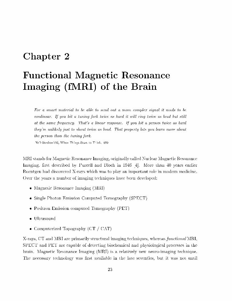
For a smart material to be able to send out a more complex signal it needs to be
nonlinear. If you hit a tuning fork twice as hard it will ring twice as loud but still
at the same frequency. That's a linear response. If you hit a person twice as hard
they're unlikely just to shout twice as loud. That property lets you learn more about
the person than the tuning fork.
-Neil Gershenfeld, When Things Start to Think,1999
MRI stands for Magnetic Resonance Imaging, originally called Nuclear Magnetic Resonance
Imaging, �rst described by Purcell and Bloch in 1946 [4]. More than 40 years earlier
Roentgen had discovered X-rays which was to play an important role in modern medicine.
Over the years a number of imaging techniques have been developed:
� Magnetic Resonance Imaging (MRI)
� Single Photon Emission Computed Tomography (SPECT)
� Positron Emission computed Tomography (PET)
� Ultrasound
� Computerized Topography (CT / CAT)
X-rays, CT and MRI are primarily structural imaging techniques, whereas functionalMRI,
SPECT and PET are capable of detecting biochemical and physiological processes in the
brain. Magnetic Resonance Imaging (MRI) is a relatively new neuro-imaging technique.
The necessary technology was �rst available in the late seventies, but it was not until
23
1981 that MRI was introduced in clinical medicine. Over the last 10-12 years techniques
that enable non-invasive whole brain measurement of physiological processes have been
developed. These methods are known as functional MRI [34]. One exciting area in fMRI
is event-related fMRI, which involves the development and application of methods based on
the transient neuronal changes associated with individual cognitive, sensory and/or motor
events [7].
The remainder of this chapter is organized as follows. The next section introduces the
concept of digital images after which we give a short description of the general principles
in MRI. Knowledge about basic MRI physics is important for the understanding of the
methods applied in this thesis. Readers that are familiar with the MRI technique may skip
this section. Finally, preprocessing of MRI-data will be brie y discussed before a section
on functional MRI concludes the chapter.
2.1 Digital Images
Digital images can be viewed as arrays of grey values in which each array element repre-
sents one point in the image. Array elements of two-dimensional images are called pixels
whereas voxels denote the volume elements in 3D. Digital volumetric images are stacks of
2-dimensional image arrays. A 2D array that is a part of a 3D image is called a slice.
Slices in 3D images can be viewed in all of the 3 orthogonal directions, regardless of the
orientation in which they originally were acquired (see Figure 2.1).
Indexing the rows and columns within each slice allows each voxel to be associated with a
unique address. More formally, a volumetric image is the set of addresses:
f(x; y; z) j 0 � x � nslices; 0 � y � nrows; 0 � z � ncolumnsg
where nslices, nrows and ncolumns denotes the number of slices, rows and columns, re-
spectively [30]. An n-dimensional digital image can be viewed as a mathematical function
f : Df ! V
in which D is a rectangular n-dimensional grid and V is a set of intensity (or grey-level)
values (see Figure 2.2).
24
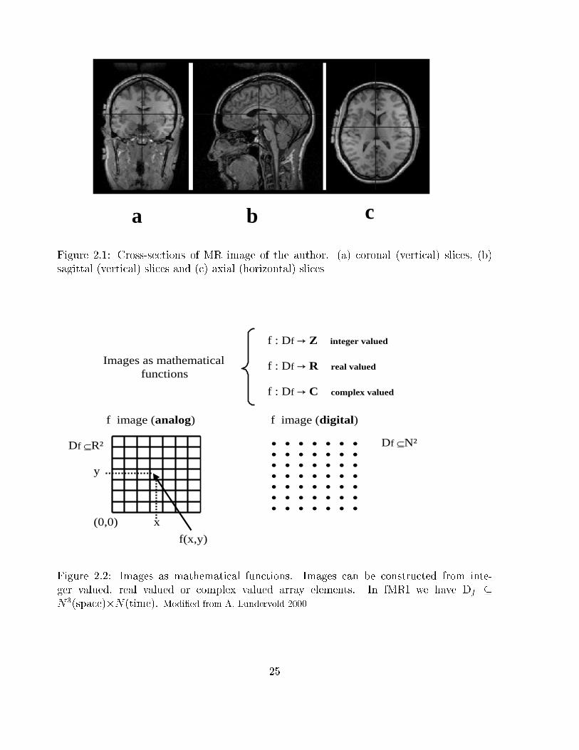
a b c
Figure 2.1: Cross-sections of MR image of the author. (a) coronal (vertical) slices, (b)
sagittal (vertical) slices and (c) axial (horizontal) slices
�������
�������
�������
�������
�������
�������
�������
(0,0)
Images as mathematical functions
f : Df � Z integer valued
f : Df � R real valued
f : Df � C complex valued
f image (analog) f image (digital)
f(x,y)
x
y
Df ⊆R² Df ⊆N²
Figure 2.2: Images as mathematical functions. Images can be constructed from inte-
ger valued, real valued or complex valued array elements. In fMRI we have Df �
N3(space)�N(time). Modi�ed from A. Lundervold 2000
25
2.2 Basic principles of MRI
In every form of X-ray imaging, a beam of X-rays passes through the body which itself
becomes a source of secondary X-rays. The contrast between body parts in X-ray imaging
is produced by the di�erent scattering and absorption of X-rays by bones and tissues. A
major limitation is, however, that exposure of body cells and tissue to large doses of X-rays
constitutes a potential health hazard. In MRI we deal with much lower energies than in
X-rays or even in visible light [21], and it is the body itself that generates the signals that
is the basis for the image acquisition. In a simple way, MRI is an interaction between an
external magnetic �eld, radio waves and nuclei in the body. Before explaining the imaging
performed by MRI a few important phenomena, such as magnetization of the body, radio
frequency excitation, and measurement of relaxation, need to be explained.
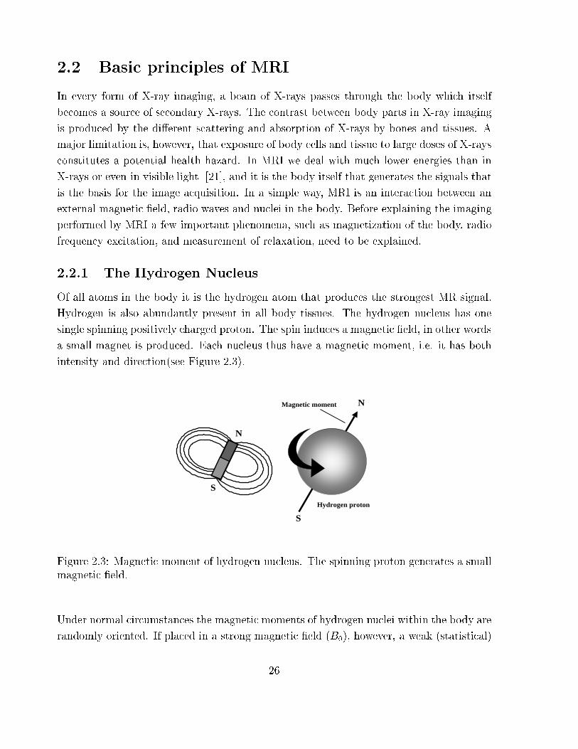
2.2.1 The Hydrogen Nucleus
Of all atoms in the body it is the hydrogen atom that produces the strongest MR signal.
Hydrogen is also abundantly present in all body tissues. The hydrogen nucleus has one
single spinning positively charged proton. The spin induces a magnetic �eld, in other words
a small magnet is produced. Each nucleus thus have a magnetic moment, i.e. it has both
intensity and direction(see Figure 2.3).
N
S
Magnetic moment
N
S
Hydrogen proton
Figure 2.3: Magnetic moment of hydrogen nucleus. The spinning proton generates a small
magnetic �eld.
Under normal circumstances the magnetic moments of hydrogen nuclei within the body are
randomly oriented. If placed in a strong magnetic �eld (B0), however, a weak (statistical)
26
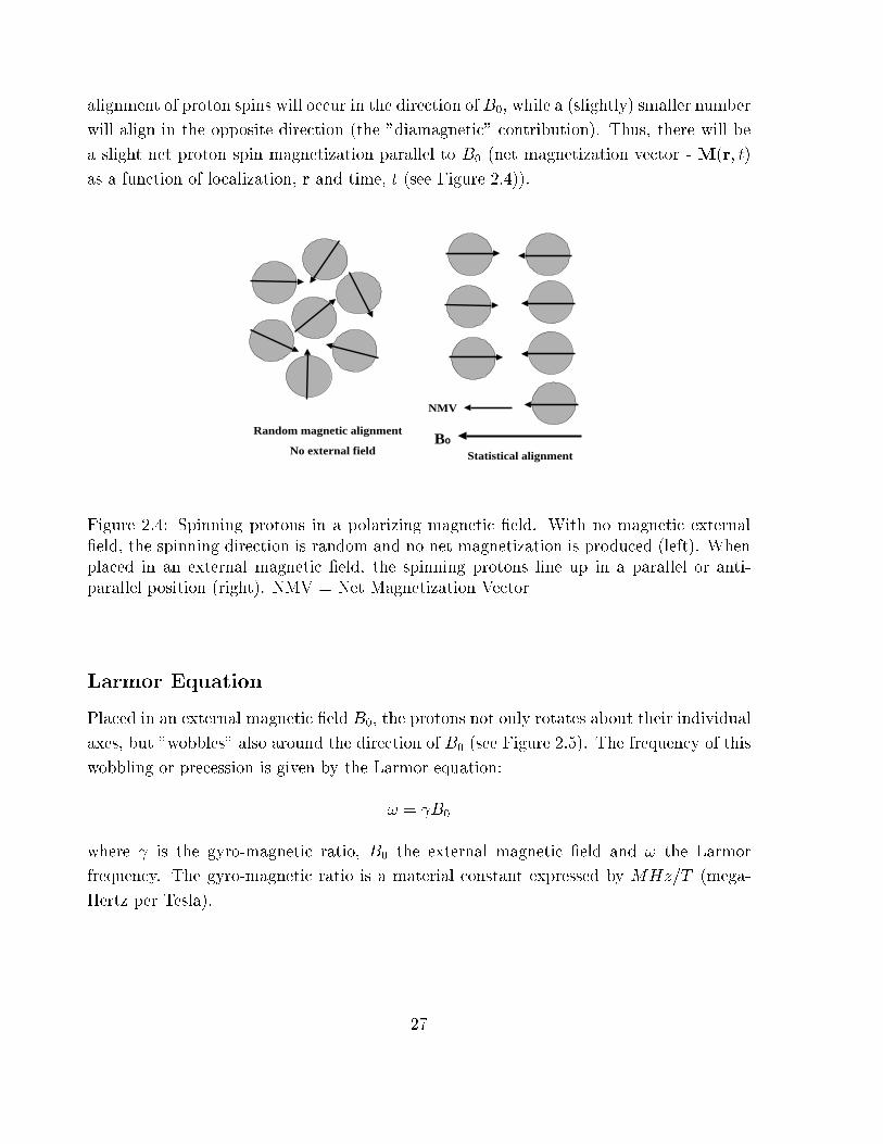
alignment of proton spins will occur in the direction of B0, while a (slightly) smaller number
will align in the opposite direction (the "diamagnetic" contribution). Thus, there will be
a slight net proton spin magnetization parallel to B0 (net magnetization vector - M(r; t)
as a function of localization, r and time, t (see Figure 2.4)).
NMV
B�Statistical alignment
Random magnetic alignment
No external field
Figure 2.4: Spinning protons in a polarizing magnetic �eld. With no magnetic external
�eld, the spinning direction is random and no net magnetization is produced (left). When
placed in an external magnetic �eld, the spinning protons line up in a parallel or anti-
parallel position (right). NMV = Net Magnetization Vector
Larmor Equation
Placed in an external magnetic �eld B0, the protons not only rotates about their individual
axes, but "wobbles" also around the direction of B0 (see Figure 2.5). The frequency of this
wobbling or precession is given by the Larmor equation:
! = B0
where is the gyro-magnetic ratio, B0 the external magnetic �eld and ! the Larmor
frequency. The gyro-magnetic ratio is a material constant expressed by MHz=T (mega-
Hertz per Tesla).
27

B�
Hydrogen nucleus
Figure 2.5: Proton precession. Spinning Protons "wobbles" around the direction of the
external magnetic �eld
2.2.2 Resonance
If a hydrogen nuclei in the magnetic �eld B0 is exposed to radio frequency radiation, RF
( by convention called the B1 �eld ) at the Larmor frequency, the nuclei will "jump" into
a higher energy state. This causes the net magnetization to spiral away from the B0 �eld
and into the transverse plane. It is in this position that the net magnetization can be
detected in MRI. The orientation of the coordinate system of the MRI scanner in relation
to the magnetic �elds is depicted in Figure 2.6.
Figure 2.6: Orientation of coordinate system of the MRI scanner and magnetic �elds. � if
the ip angle and NMV is the Net Magnetization Vector, M(r; t).
The application of an RF-pulse that causes resonance is called excitation. The angle �
is the so called ip angle, and its magnitude depends on the amplitude and duration of
the RF-pulse. Another result of the RF-pulse is that the magnetic moments of the nuclei
within the transverse plane move in such a way that they are in phase with each other, i.e
28

they become synchronized. A receiver coil placed in an area with excitated in-phase nuclei,
will receive a signal whenever the in-phase magnetization cuts the coil.
2.2.3 Imaging hardware
The MRI scanner consists of four components : the magnet, gradient coils, radio frequency
transmitter and a computer. The magnet is of course the most important component of
the equipment. Strong magnetic �elds are required to produce good MR images. There are
basically two ways of obtaining the required magnetic �eld, either by using a permanent
magnet or an electromagnet. The last method is used for all scanners with a �eld strength
above 0.5 Tesla. In addition to the coils that produce the main magnetic �eld, B0, there
are other coils that induce smaller magnetic �elds, which are gradient coils for producing
a gradient �eld ( in B0) in the X, Y, and Z directions. Within the gradient coils there is
also the RF coil which produces the B1 magnetic �eld. Finally, the computer controls all
components of the scanner and the operator gives input to the computer through a control
console. Figure 2.7 gives a schematic view of a MRI scanner.
B�
RF pulse
generator
RF pulse
controller
Gradient
controller
Coils that generate the static
magnetic field B�, gradients
and RF transmitter
RFamplifier
Signal processing
Image reconstruction
Work station
Figure 2.7: Schematic view of a MRI scanner
29

2.2.4 Gradients
The gradient coils produce the gradients in the B0 magnetic �eld. A gradient is simply a
magnetic �eld that changes, usually linearly, from point to point. Gradients in the magnetic
�eld causes each of the regions of spin to experience a unique magnetic �eld, determining
their position in the image. The symbols of the magnetic �eld gradient in the z, y, and x
directions are Gz, Gy, and Gx. The three gradients are referred to as :
1. the slice select gradient
2. the phase encoding gradient
3. the frequency encoding gradient
In the following Gz refers to the slice select gradient, Gy to the phase encoding gradi-
ent, and Gx to the frequency encoding gradient. This will result in a tranverse view of the
object. A unique property of MRI is, however, that the Gy and Gx also can be employed
to select a slice, thereby producing images from other angles, including oblique views.
Slice selection
Slice selection is the excitation of spinning nuclei in a plane through the object. When
the slice encoding gradient is switched on, the magnetic �eld strength is altered in a linear
way such that each point along the z-axis has a speci�c precessional frequency. A slice
can then be selected by transmitting an RF pulse with a bandwidth coincident with the
Larmor frequency of a particular slice. The slice select gradient, Gz, is turned on during
the period that the RF pulse is applied. The thickness of an image slice is determined by
the range of frequencies (bandwidth) of the RF pulse.
Spatial encoding
After selecting a slice, we need to know how much signal comes from each voxel (volume
element) in the slice. This is accomplished with frequency and phase encoding. We begin to
locate the signal along the X-axis. By switching on the frequency encoding gradient a linear
frequency di�erence along the X-axis occurs. We can now locate a signal along the axis
according to its frequency. The frequency encoding gradient is switched on when the signal
is received. We now need to perform the phase encoding which is the localization of the
signal along the remaining y-axis. As with the frequency encoding gradient, the magnetic
�eld strength along the axis of the gradient is altered when the phase encoding gradient is
turned on. The gradient Gy is turned on for a short period prior to signal measurement.
30
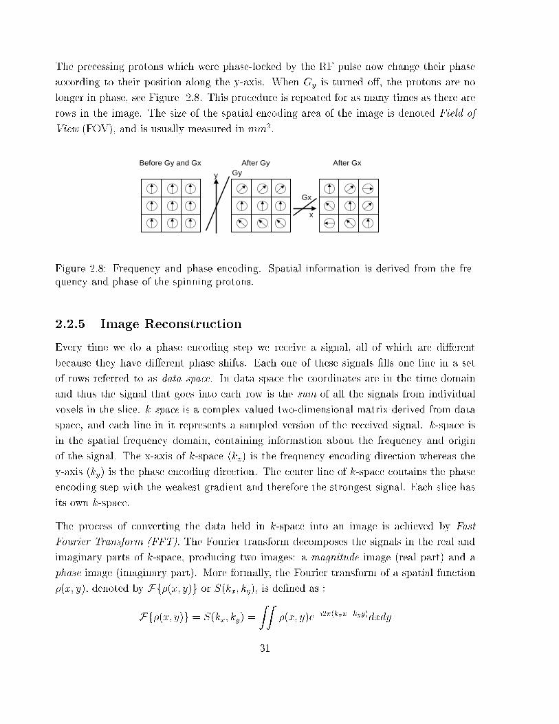
The precessing protons which were phase-locked by the RF pulse now change their phase
according to their position along the y-axis. When Gy is turned o�, the protons are no
longer in phase, see Figure 2.8. This procedure is repeated for as many times as there are
rows in the image. The size of the spatial encoding area of the image is denoted Field of
View (FOV), and is usually measured in mm2.
x
y Gy
Gx
Before Gy and Gx After Gy After Gx
Figure 2.8: Frequency and phase encoding. Spatial information is derived from the fre-
quency and phase of the spinning protons.
2.2.5 Image Reconstruction
Every time we do a phase encoding step we receive a signal, all of which are di�erent
because they have di�erent phase shifts. Each one of these signals �lls one line in a set
of rows referred to as data space. In data space the coordinates are in the time domain
and thus the signal that goes into each row is the sum of all the signals from individual
voxels in the slice. k-space is a complex valued two-dimensional matrix derived from data
space, and each line in it represents a sampled version of the received signal. k-space is
in the spatial frequency domain, containing information about the frequency and origin
of the signal. The x-axis of k-space (kx) is the frequency encoding direction whereas the
y-axis (ky) is the phase encoding direction. The center line of k-space contains the phase
encoding step with the weakest gradient and therefore the strongest signal. Each slice has
its own k-space.
The process of converting the data held in k-space into an image is achieved by Fast
Fourier Transform (FFT). The Fourier transform decomposes the signals in the real and
imaginary parts of k-space, producing two images: a magnitude image (real part) and a
phase image (imaginary part). More formally, the Fourier transform of a spatial function
�(x; y), denoted by Ff�(x; y)g or S(kx; ky), is de�ned as :
Ff�(x; y)g = S(kx; ky) =
ZZ�(x; y)e�{2�(kxx+kyy)dxdy
31

where ky and kx are given by
kx = t
2�Gx; ky =
t
2�Gy:
For our purpose S(kx; ky) are the acquired experimental data measured in k-space while
�(x; y) is the desired image function representing for example the spin density function.
Given S(kx; ky), we can recover �(x; y) using the inverse Fourier transform:
�(x; y) = F�1fS(kx; ky)g =
ZZS(kx; ky)e
�{2�(kxx+kyy)dkxdky
The magnitude image is used for visual inspection while the phase image, which is more
sensitive to moving spins and magnetic �eld inhomogeneities, is useful for cases in which
the direction is important, such as when measuring ow (see Figure 2.9).
B0
ω
M(r,t)
y
x2D FFT
B1
RF
z
transmit/receive
Mag = (X2 + Y2)½
Pha = atan(Y/X)
X
Y
kx
kx
ky
ky R
I
K = R + i*I;C = ifft2(K); Z = fftshift(C);X = real(Z); Y = imag(Z);A = abs(Z); P = atan( Y ./ X);
k-space
“Imaginary” channel
“Real”channel
Figure 2.9: MR image formation. X is the real and Y is the imaginary part of the
reconstructed image. Mag is the magnitude image whereas Pha is the phase image. In
this thesis we shall use the magnitude image. x; y; z are scanner coordinates and kx; ky are
spatial frequency coordinates. (Modi�ed from A. Lundervold, 2000)
32

2.2.6 Relaxation and Tissue Contrast
Whenever the RF-pulse is cut o�, B0 will regain its dominating in uence on the net mag-
netization. This process, in which the net magnetization looses its energy, is termed relax-
ation. Relaxation consists of two independent processes :
� T1 recovery is the process in which the net magnetization returns to its ground
state in the direction of the main magnetic �eld B0. In the process of returning to
their initial energy level, the protons loose energy to the surrounding environment or
lattice (spin-lattice relaxation). The rate of this recovery is an exponential process,
with time constant T1.
� T2 decay is the loss of transverse magnetization. It occurs when the magnetic �elds
interact with each other (spin-spin interaction) and exchange energy, resulting in a
spin de-phasing. Like in T1 recovery the rate of the T2 decay is characterized with
a time constant T2.
During relaxation, signals can be detected by the receiver coil within the MR scanner. Since
T1 and T2 relaxation times depend on the biological materials, tissues of di�erent nature
will emit di�erent signals. A tissue with a high signal has a large transverse component of
magnetization and is displayed as white areas in the image. In contrast, a small transverse
component will result in a low signal and appear therefore as dark areas in the image. The
two substances that di�er the most are fat and water. The T1 recovery and T2 decay
of fat is short, whereas both T1 and T2 of water are long. T1-weighted images will thus
display water as dark areas and fat as white areas. In T2-weighted images, however, fat
will produce a low signal resulting in dark areas whilst water with the stronger signal, will
appear as white areas. A list of T1 and T2 relaxation times of brain tissues are listed in
Table 2.1.
Tissue T1 (ms) T2 (ms)
Grey Matter 1000 106
White Matter 650 69
Fat 260 60
Cerebrospinal Fluid 4000 2300
Table 2.1: T1 and T2 relaxation times of brain tissues at 1.5 Tesla
33

In order to create images, we need a sequence that appropriately alternates between an RF
pulse and relaxation. The time between two successive RF pulses is denoted TR, while TE
is the time interval between the RF pulse and the signal measurement. Both TE and TR
are conventionally measured in milliseconds. We can obtain T1 weighted or T2 weighted
images by choosing appropriate settings for TR and TE. Short TE and short TR will
produce a T1 weighted image, whereas long TE and long TR will produce a T2 weighted
image.
RF pulse
RF pulse RF pulse RF pulse
TR TR
RF pulse RF pulse
signal signal
TE TE
Figure 2.10: TE (echo time) and TR (repetition time). The repetition time is the time
interval between each RF cycle whereas echo time is de�ned as the time interval between
the RF pulse and the signal measurement.
T2* weighted images
T2 decay depends on the spin-spin interaction in the tissue (internal inhomogeneities).
There is another phenomenon that makes spin get out of phase, namely inhomogeneity of
the external magnetic �eld. T2* decay depends on both the external magnetic �eld and
on the spin-spin interactions. T2* relaxation time is always shorter than T2.
2.2.7 Pulse Sequences
A pulse sequence is a sequence of RF-pulses and gradients applied repeatedly during the
process of producing an MR image. The choice of the parameters TE and TR determines
the weighting of the images, whereas the quality of the images depends on several factors:
� Signal to Noise Ratio (SNR)
34

� Contrast to Noise Ratio (CNR)
� spatial resolution
� scan time
SNR is the ratio of the amplitude of the received signal to the average amplitude of the
noise. CNR is de�ned as the di�erence in the SNR between two adjacent areas. Both
SNR and CNR will be discussed in Section 2.2.8. The spatial resolution is controlled by
voxel size, small voxels give a good spatial resolution since small structures can be easily
di�erentiated. The scan time is the time it takes to complete image acquisition. A long
scan time increases the chance of the patient moving inside the scanner, thereby reducing
image quality.
Spin Echo Sequences (SE)
As described earlier, the T2* relaxation has two components, inhomogeneities caused by
the external magnetic �eld and inhomogeneities on the molecular level. It is this last
component that is interesting from a medical view. Consequently, we seek to produce an
image that re ects only the di�erences in T2 contrast, disregarding the external component
of T2*. The external magnetic inhomogeneities are constant over time, and are therefore
simple to eliminate. In the SE sequence a 90Æ RF pulse is followed by a 180Æ RF pulse.
After the 90Æ pulse we will detect a signal which gradually decays due to the T2* relaxation
e�ect. After the 180Æ pulse, however, the signal gradually returns as the protons move back
in phase with each other. This signal is called an echo and the pulse sequence is therefore
called a Spin-Echo sequence. The purpose of the SE sequence is to separate the two
components of T2*. Due to the microscopic component of T2*, which varies over time,
the protons does not fully return back in phase with each other after the 180Æ pulse. This
means that the echo-signal will rely on the microscopic, tissue-dependent T2 values and
not on the external magnetic �eld inhomogeneities. The intensity of the signal will thus be
a function of the tissue's T2 values and the time between the 90Æ pulse and the 180Æ pulse.
If the TE's are close to zero, the signal will be sampled directly after the 90Æ pulse. At
this point the T2 relaxation has no e�ect on the signal, and di�erences in signal intensity
depend therefore primarily on the proton density of the tissue. A voxel with many protons
will result in a stronger signal (and consequently also a stronger echo signal) than a voxel
with a smaller number of protons. MR images that display di�erences in proton density
are called proton density images.
35

An MR image that emphasizes the di�erences in the echo signal due to T1 di�erences of
the tissue, is a T1 weighted image. To produce a T1 weighted image from the SE sequence,
two criteria need to be satis�ed. First, TR must be relatively short, such that there is a
marked di�erence between available net magnetic moments for di�erent types of tissue
(this usually means a TR of 300-800 milliseconds). Secondly, TE must be short in order
to avoid T2 contrast in the image.
RF
Slice
Frequency
Phase
Signal
90° 180°
time
Spin echo
Figure 2.11: Spin Echo sequence
Gradient Echo Sequences (GRE)
A major drawback with the SE sequence is that it is time consuming. The overall acquisi-
tion time is directly proportional to the length of TR, which therefore should be reduced
to a minimum. The challenge is to produce an echo without the 180Æ RF pulse, and as
the name (Gradient Echo Sequences) implies, the gradients are also used for this purpose.
Consider a gradient that is kept constant after the 90Æ RF pulse; the protons are de-phasing
and the NMR signal decreasing. If the gradient after a time t is "reversed", the protons
will move back in phase, and an echo is produced. This echo does, however, depend on
both components of T2*, and as such it is not a "true" T2 contrast. The reason for not
using the original signal is that the echo signal contains more information than a NMR
signal, and is therefore better suited for image construction. Another characteristic of the
GRE sequence is an RF pulse yielding a smaller ip angle than the usual 90Æ RF pulse.
Short TR and a ip angle < 90Æ results in a small net magnetism, and subsequently a
36

smaller signal than in a SE sequence. As a result, one should expect a poor Signal to
Noise Ratio. This is compensated, though, by the higher temporal resolution in the GRE
sequence, which makes it possible to increase the number of scans and thereby enhancing
the statistical power.
Advanced Imaging Techniques
Most available imaging techniques are modi�cations of Spin Echo and/or Gradient Echo
procedures. In some fast scanning techniques, multiple echoes with individual phase en-
coding within each TR are generated(examples are Turbo or Fast spin echo sequences and
Echo Planar Imaging - EPI). Single-shot techniques allow for all the lines of K space to be
acquired in one TR, thereby reducing scan times even further.
Within the gradient echo (GRE) sequences there is a wide range of variations compared to
the spin echo (SE) sequences. Not only is the basic sequence varied by adding dephasing or
rephasing gradients at the end of the sequence, but there are also the TR, TE and the ip
angle to consider. For the gradient echo sequence FLASH (Fast low-angle Shot), a larger
ip angle give more T1 weighting to the image, whereas a smaller ip angle give more T2
or actually T2* weighting to the images. The contrast between di�erent tissues in FLASH
images is such that they are well suited for anatomical inspection(see Figure 2.13).
EPI
RF
Gz
Gy
Gx
echoes
readout
slice select
phase encode
Figure 2.12: Echo Planar Imaging Sequence
Echo planar imaging (EPI)(see Figure 2.12) is another gradient echo technique related
to fast gradient echo imaging. In EPI the entire set of phase steps is acquired during
37

one acquisition TR. To accomplished this, the frequency encoding gradient is rapidly and
repeatedly reversed. EPI sequences may use only gradient echoes or combine a spin echo
with the train of gradient echoes. Echo planar images can be acquired in the order of
100ms or less and are therefore useful for detecting rapidly changing processes like those
of the brain. Whole brain volumes, consisting of multiple 2-dimensional images (slices),
may thus be acquired in 1-2 seconds depending on the number of slices (see Figure 2.14).
In all, most of the imaging methods used for functional MRI are based on the principles
of EPI.
(a). FLASH
(b). FLASH
(c). EPI
Figure 2.13: FLASH versus EPI. (a) FLASH image, sagittal slice, (b) FLASH image, axial
slice, (c) EPI, axial slice
38

Figure 2.14: Multislice EPI
2.2.8 Image Noise and Artifacts
There are two main sources of image noise, random noise, and structured noise [23].
Random noise is time invariant and occurs at all frequencies. For k-space values (kx; ky)
the measured signal, sm, can be described as:
sm(kx; ky) = st(kx; ky) + "(kx; ky)
where st is the true signal. The noise term, "(kx; ky), derives from random uctuations gen-
erated by the subject within the scanner as well as background noise from the equipment.
The noise variance is given by :
�2therm(kx; ky) = �
2bodytissue(kx; ky) + �
2coil(kx; ky) + �
2electronics(kx; ky)
Signal to Noise Ratio
Signal to Noise Ratio (SNR) is the ratio of the amplitude of the received signal to the
amplitude of the noise. The signal, S, is dependent on the stimuli and is therefore increased
39

or decreased relative to the noise. Signal to Noise Ratio can be formulated as :
SNR �S
�0
where �0 denotes the noise standard deviation. There are a number of parameters that
in uence the Signal to Noise Ratio, and they should be chosen so that SNR is maximized.
The relationship between SNR and these parameters is given by :
SNR / (voxelvolume)
q(Ny)(NEX)=(BW ):
SNR is thus increased by an increase in voxel volume, the number of acquisitions per phase
encoding step (Ny) or the number of scans/excitations (NEX), or decreased bandwidth
(BW).
Contrast to Noise Ratio
Contrast to Noise Ratio (CNR) depends on the same factors as SNR. The SNR is de�ned
by the di�erence in SNR between two neighbouring areas. A high CNR is essential for the
ability to distinguish pathology from normal tissue. A measure of �0 can be achieved by
computing the mean of a region outside the object.
Contrast between tissue A and B and the CNR is given by the formulas :
CAB � SA � SB
and
CNRAB �CAB
�0=
SA � SB
�0= SNRA � SNRB
Image artifacts
Image artifacts, which to some degree are present in all MR images, arise from a variety
of causes, including the imaging technique itself and natural processes or properties of the
human body. Some artifacts may be avoided, while others can only be reduced. A brief
description of the most common artifacts is given below.
� Motion
Motion artifact is caused by the subject within the scanner. These are either volun-
tary (random) or involuntary (periodic). Random motion such as breathing, cough-
ing, swallowing and changing position generally causes blurring in the images.
Periodic motion, which produces an artifact known as ghosting, arises from periodic
pulsation, for example from vessels or cerebrospinal uid. Mechanical vibrations,
receiver coil and uctuations of the magnetic �eld may also produce ghosts.
40

� Geometrical distortions
The various processes that distort the magnetic �eld strength also lead to geometrical
distortions of the image. Sources of geometrical distortion include inhomogeneity in
the external magnetic �eld, spatial variations in magnetic susceptibility and nonlin-
earity in the magnetic �eld gradients [45]. The fMRI method of choice, EPI (see
Section 2.2.7), produces images that contain a signi�cant amount of T2* decay. The
technique is thus sensitive to the �eld inhomogeneities found in tissue, air and bone.
Di�erence in magnetic susceptibility between air and body tissue and between dif-
ferent body tissues cause signal loss and distortion at the boundaries of the tissues.
The EPI technique is especially subject to geometrical distortions because of the long
read-out time after each RF pulse.
� Wrap around
Anatomy outside the selected imaging area (FOV) produces signals which will be
detected if the distance to the receiver coil is small. Wrap around or aliasing artifact
arise when these structures are mapped inside the FOV. The part of the anatomy
that lies outside the FOV is projected on to the other side of the image. Anti-aliasing
methods can be applied to compensate for this wrapping e�ect.
This concludes the MR physics section. Further reading on the subject can be found in
[21] and [43].
2.3 Preprocessing of fMRI data
Before the sampled image time series can be subject to statistical analysis, a few prepro-
cessing steps are required.
� Image registration is the process of geometrical transformations applied to an image
when aligning it spatially to another image. This procedure is necessary to minimize
the e�ects of motion in series of images, as in fMRI where a single session may consist
of several hundred EPI images. Aligning images acquired of a subject in di�erent
MR sessions is another important area of application.
� Normalization maps a brain image into a standardized reference space. The most
commonly used coordinate system within brain imaging is that described by the
atlas of Talairach and Tournoux [42]. Normalization is useful for the comparison
of di�erent subjects and databases. Activations can be reported according to their
41
coordinates within the standard space. Due to the fact that there is no one-to-one
mapping of cortical structures between subjects, matching is only possible on a coarse
scale [1].
� Smoothing is a low pass �ltering (e.g. Gaussian) which convolves the voxels in the
EPI images with a kernel shaped according to the applied �lter. Smoothing improves
the image quality by increasing the Signal to Noise Ratio [46].
� Slice-timing is a procedure for correcting er-fMRI time series data for the di�erences
in image acquisition time between slices.
Upon completing the preprocessing procedure the functional data-set can be submitted
to statistical analysis and the results superimposed on a structural high resolution image.
The datasets used in this thesis has been preprocessed with The Statistical Parametric
Mapping (SPM99) software toolbox (see Appendix A.3).
42

2.4 Functional Magnetic Resonance Imaging (fMRI)
We are what we think.
All that we are arises with our thoughts.
With our thoughts, we make the world.
Buddha
Functional Magnetic Resonance Imaging (fMRI) produces brain images that re ect neu-
ronal activity due to sensory, cognitive or motor tasks [16]. The fMRI technique, which is
about to enter its second decade as a scienti�c discipline, has dramatically expanded the
possibilities for the study of human brain function and pathology. Since it is non-invasive
and has no signi�cant risks, it is widely applicable and a considerable number of studies
have been conducted in numerous MR laboratories. The �rst fMRI experiments used an
exogenous contrast agent, but this was soon replaced by the so-called blood oxygenation
level dependent (BOLD) contrast. A typical fMRI experiment measures the correlation
between the BOLD response and a stimulus regime.
2.4.1 Blood Oxygenation Level Dependent (BOLD) Contrast
The BOLD-contrast arises form the magnetic properties of blood, �rst described by Paul-
ing and Coryell in 1936 [37], and is the most widely used fMRI-method for detection of
brain activation. Haemoglobin, the major component of the red blood cells, is an organic
molecule that transports oxygen in the vascular system of the body. As blood perfuses
from the arterial side of the capillary bed to the venous side, oxygen dissociates from the
haemoglobin supplying the tissue with oxygen. Deoxyhaemoglobin (haemoglobin without
oxygen) has, due to unpaired electrons, a relatively large magnetic moment. When oxy-
gen binds to haemoglobin (oxyhaemoglobin), the unpaired electrons are transferred to the
oxygen molecules, eliminating the magnetic moment. Oxyhaemoglobin is therefore dia-
magnetic, whereas deoxyhaemoglobin is paramagnetic, thus creating microscopic magnetic
�eld gradients in its vicinity yielding di�erent signal intensities (see Figure 2.15). This
mechanism give rise to BOLD-contrast on T2* weighted images (see Section 2.2.6). At
rest (periods of no stimuli) the amount of deoxyhaemoglobin and oxyhaemoglobin are sim-
ilar, but during brain activity, both blood ow and metabolism are increased and more
oxygen is extracted from the capillaries. The increase in delivered oxygen, however, exceeds
the metabolic need, leading to an increase in the oxyhaemoglobin content and a relative
43

decrease in the fraction of deoxyhaemoglobin in the venous part of the micro-circulation
of the capillary bed [34].
Resting state
Stimulated state
HbO2 Hbarterial venousBOLD Contrast
Figure 2.15: Haemoglobin concentration in blood during rest and activation. During stim-
ulus induced activation there will be a higher proportion of oxyhaemoglobin (white) on
the venous side of the capillary bed, thereby increasing the MR signal intensity from this
region.
The amount of deoxyhaemoglobin thus depends on physiological factors such as the change
in Cerebral Blood Flow (CBF), the rate at which oxygen is metabolized (CMRO2) and
the change in Cerebral Blood Volume (CBV). The ratio of deoxyhaemoglobin to oxy-
haemoglobin is the basis for the BOLD contrast. Vessels that contain a signi�cant amount
of deoxyhaemoglobin creates, due to its paramagnetic nature, local �eld inhomogeneities
causing increased spin-spin dephasing. During activity the relative amount of deoxy-
haemoglobin decreases leading to a decrease in dephasing and hence an increase in signal
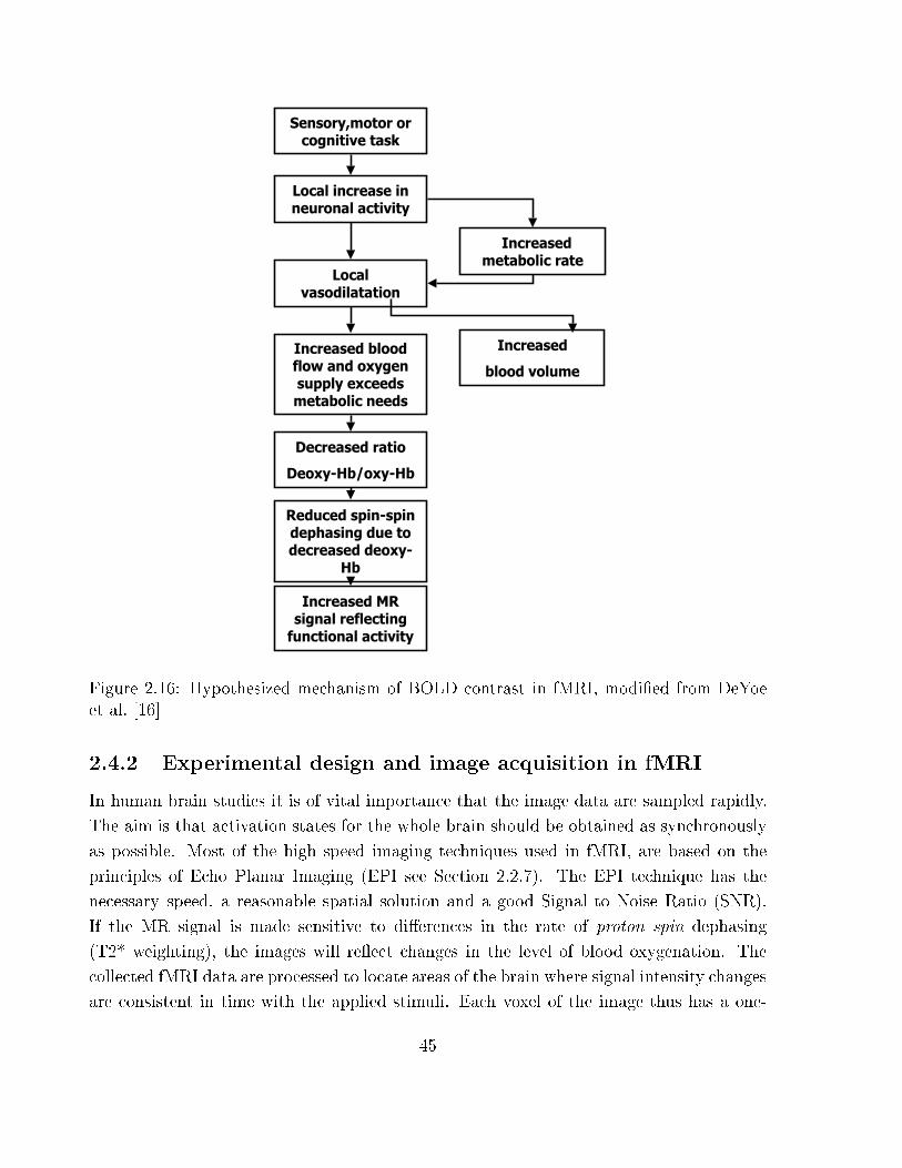
intensity (see Figure 2.16). The mechanism behind the BOLD response are very complex
and are subject to both underlying physiological processes and imaging physics events [24].
A voxel in an fMRI experiment usually has a size in the order of 3mm� 3mm� 3mm, it
is thus a problem that a large number of voxels contain vessels of varying sizes, ranging
from small capillaries to larger draining veins. The exact relationship between this under-
lying vascular geometry, distribution of deoxyhaemoglobin and signal change has yet to be
established.
44
���������
���� �����
���������������������
����� �������������
��������������������������� ���
����������������������������������������������������
������������������������� �������������� ������
�
��������������
�������������
����������������������������������������� ���
������!�������������� ����"
Figure 2.16: Hypothesized mechanism of BOLD contrast in fMRI, modi�ed from DeYoe
et al. [16]
2.4.2 Experimental design and image acquisition in fMRI
In human brain studies it is of vital importance that the image data are sampled rapidly.
The aim is that activation states for the whole brain should be obtained as synchronously
as possible. Most of the high speed imaging techniques used in fMRI, are based on the
principles of Echo Planar Imaging (EPI see Section 2.2.7). The EPI technique has the
necessary speed, a reasonable spatial solution and a good Signal to Noise Ratio (SNR).
If the MR signal is made sensitive to di�erences in the rate of proton spin dephasing
(T2* weighting), the images will re ect changes in the level of blood oxygenation. The
collected fMRI data are processed to locate areas of the brain where signal intensity changes
are consistent in time with the applied stimuli. Each voxel of the image thus has a one-
45

dimensional time series, with length equal to number of scans, associated with it. To detect
stimulus related activity, each voxel time series can be compared with a predicted/expected
response function.
During an experiment the subject lies within the scanner viewing a screen illuminated by
an LCD video projector, listens to auditory input via headphones, or performs some other
form of task, while a sequence of images are sampled. The presentation of stimuli and
the scan sequence are synchronized, either manually or by a computer. Brain activation
paradigms must be designed so that they reliably detect and isolate the neural changes
associated with cognitive, sensory, or motor events. A typical fMRI experiment applies a
speci�c set of assumptions to localize relative di�erences in brain activity between active
and baseline tasks. fMRI designs are either blocked, with relatively long periods of stimuli
followed by intervals of rest, or event-related, in which the individual trials are isolated.
2.4.3 Blocked vs. Event-Related design
The block design is traditionally the most common design in fMRI experiments. In blocked
task paradigms the MR images are acquired continuously while subjects are presented with
blocks of stimulation (duration of approximately 30 seconds each), intermixed with rest
intervals. Blocks of trials, condition versus rest or condition 1 versus condition 2, are then
compared using statistical tests.
More formally, in a blocked trial design, each voxel in the image is a function, f(x; y; z; t) 2
R, of location and time, where x denotes the column, y the row and z the slice in the volume
sampled at time t. There are n blocks with k trials in each block where block i represents
the condition ci 2 f1::mg, and t 2 ft11; :::; t1k; :::; tn1; :::; tnkg (see Figure 2.17).
Since fMRI noise is assumed to be normally distributed and stationary in time [27], aver-
aging across trials in the blocked trial design increases the Signal to Noise Ratio (SNR, see
Section 2.2.8). Time dependent behavior and brain function, such as learning, alterations
in strategy and errors, or habituation (all which are common in cognition) may, however,
change during a block of repeated trials. In such cases the averaging approach looses unique
information due to the e�ects of learning and strategy [32].
Event-related (or single trial) functional Magnetic Resonance Imaging (er-fMRI) is a rel-
atively new experimental design that allows di�erent trials to be presented in arbitrary
sequences, thereby eliminating the potential problems as mentioned above. Several stud-
ies, e.g. [5, 14, 29, 27, 11, 8, 38] has demonstrated that er-fMRI has the ability to detect
activation from very brief periods of stimulation, in the order of ms. These procedures also
46

show that the BOLD response is delayed in relation to the neuronal activity, extending over
several seconds. These �ndings represents a challenge to er-fMRI since BOLD responses to
adjacent trials may overlap. A solution is to space the trials so far apart that the BOLD
response has returned to baseline after each trial. This does, however, severely limit the
total number of trials and hence the number of trials upon which to average, decreasing
the Signal to Noise Ratio. It has been suggested that trials be spaced close together, only
a few seconds apart, subsequently applying methods for removal of overlap between the
BOLD responses[14].
3D+time
TIMESPACE
Condition A
Condition B
Condition BCondition A
Condition B
Block
Event-related
Block 1 Block n
Condition
A
Condition
B
Condition
B
time
A A AB BCondition
Blocked
Figure 2.17: Blocked vs. Event-Related design. In fMRI experiments with a block design
subjects are presented with blocks of stimulation intermixed with resting intervals whereas
in event-related fMRI single trials are presented in arbitrary sequences.
47

48

Part II
Theory
49

50

Chapter 3
Physiological models of the BOLD
response
Buckner et al. [7] gives two key characteristics of the BOLD response:
- it can be elicited following brief periods of neuronal activity, and
- it can be characterized by a well-behaved and reliable impulse function.
Knowledge about the properties of the BOLD response is essential to both experimental
design and analysis of er-fMRI data.
3.1 Characteristics of the BOLD response
At the onset of neuronal activity the oxidative metabolism is immediately upregulated, the
increase in cerebral blood ow, however, takes somewhat longer. This leads to an initial
increase in the relative amount of venous deoxyhaemoglobin and thus increased spin-spin
dephasing resulting in a decreasing MR signal [22, 27]. As the regional cerebral blood ow
and subsequently the amount of oxyhaemoglobin increases, the ratio of deoxyhaemoglobin
to oxyhaemoglobin decreases leading to reduced spin-spin dephasing and consequently an
increasing MR signal (see Section 2.4.1). This is consistent with the observed BOLD
response, which in the context of a brief �xed interval of stimulation has a small signal
decrease of about 1 sec duration, after which it increases and reaches a peak after 4-8
seconds. Although complete return to baseline may take as long as 30 seconds, the robust
response generally evolves over the �rst 10-12 seconds [7, 2, 16, 24, 9]. At the end of
the response the signal has been observed to dip below baseline and remain depressed
for several seconds [27, 9]. Buxton et al. [10] suggests that changes in the blood volume
passively follows the blood ow changes and that the post-stimulus undershoot simply may
51

signal
time
peak response
rise time
pre-under-shot
base-line
neuronal activity
5 s 10 s 15 s 20 s
fall time
post-undershot
Figure 3.1: Signal time course of the BOLD response. The pre-undershoot is interpreted
to arise from an initial increase in the relative amount of deoxyhaemoglobin due to a
delayed increase in blood ow. Rise and fall times are the times it takes for a signal to
reach its maximum intensity, or in the latter case, return to baseline. Peak response is
the time period of maximum signal intensity. Post-undershoot has been interpreted as
secondary e�ects that does not re ect the more basic physiological changes in ow and
oxygen metabolism.
be a secondary e�ect which therefore does not re ect the more basic physiological changes
in ow and oxygen metabolism.
The basic shape and timing of the haemodynamic response for similar regions of the cortex
is reported to be broadly similar across subjects (see Figure 3.1). The temporal properties
of the BOLD response can, however, vary in timing from brain region to brain region, also
within the same subject [7].
BOLD responses which arise early following a brief stimuli are most often asymmetric,
with a shorter rising than falling edge, while late and wide BOLD responses tend to be
more symmetric [28]. The sources of these di�erences in the haemodynamic response still
remain unclear, but may originate from di�erential sampling of vessels across regions or
from delays in the underlying neuronal activity [6]. Physiological factors such as heart
rate, blood pressure and perfusion may also in uence the shape of the BOLD-response.
Respiration and the cardiac cycle causes periodic changes in blood volume. Furthermore,
the vasculature di�ers from voxel to voxel, resulting in di�erent BOLD-responses even if
52

neuronal activity is the same. These issues must be considered before comparing response
magnitude and timing between locations and subjects.
The rate at which the EPI series are sampled is of the order of 100 ms per slice or less
whereas the response to a single trial/event evolves over several sampling intervals. Com-
pared to the evoked neuronal activation, the measured BOLD response is thus dispersed
and displaced in time. A haemodynamic response function (HRF) is a model function that
attempts to describe the physiological response to sensory, motor or cognitive stimuli. To
measure the correlation between the stimuli and the BOLD response, the stimuli parameter
should be subject to the same delay and dispersion as that intervening between neuronal
activity and the BOLD response. The correlation of interest then, is between the sampled
fMRI signal intensity time-series and the input stimulus function convolved with the HRF.
Since the mechanism of coupling between neuronal responses and haemodynamics are not
well understood, there is currently no exact model of the BOLD response. Several descrip-
tive and/or physiological approaches have nevertheless been proposed for the modeling of
the BOLD response. An advantage of using model functions is the possibility to derive
physiologically meaningful parameters.
One simple parametric modeling approach is to characterize the HRF by two parameters:
- lag - which represents the time delay between neural activations and the maximum
haemodynamic response, and
- dispersion - which is proportional to the duration of the haemodynamic response.
The HRF can then be approximated by appropriately setting the parameters in the chosen
parametric function. The values of the parameters are determined either by
- simple speci�cation, i.e to �nd a distribution that "looks like" the observed BOLD
response, or by
- estimation from the data
A key question is to what extent the underlying neuronal activation can be inferred from
the shape of the BOLD response, e.g. how does a stronger and/or prolonged neuronal
activation a�ect the BOLD response? The experimental conditions clearly in uence both
onset and duration of the response, and must therefore be considered in the modulation of
the response function. Overlapping responses may severely distort the individual responses
to temporal adjacent trials, and is therefore a potential challenge in er-fMRI. The obvious
solution would be to place trials suÆciently far apart, thereby avoiding the problem but
53

also decreasing the number of trials per time unit in the particular scanning session. An
alternative approach involves methods for resolving overlap between closely spaced trials [7,
14]. In these event-related fMRI experiments trials are presented as close as 2 sec or less
apart, and consequently there is no time for baseline return between successive trials. The
resulting summation of the haemodynamic responses have been found to be approximately
linear [5, 14]. There seems, however, to be a critical stimulation frequency where the
measured signal saturate. Whether these nonlinear e�ects occur on a neuronal level and/or
a haemodynamic level is still unclear. Thus, it is not known whether the underlying
neuronal activity is itself linearly additive across time and trials. In order to estimate and
remove overlap in the BOLD response, a model for how the measured response relates to
the response of each individual event is required. Such a model is presented in Section 4.2.
3.2 Simple parameterizations of the BOLD-time course
The measured fMRI signal, y, depends on the type of stimulus, brain site, time in stimulus
history (e.g. neural adaptation), individual processing abilities as well as undesirable e�ects
such as body motion, scanner instabilities, physiological and electronic noise, etc. The
undesirable e�ects, which to some extent is reduced during preprocessing of the acquired
data, can collectively be modeled as a stochastic part, �. The HRF is a deterministic
function, g(t; �) in which � = (�1; : : : ; �p) is a parameters vector of length p. We introduce
a matrix y for a single experimental run consisting of l discrete time samples in a brain
region consisting of k voxels:
y =
266664
y11 y12 ::: ::: y1l
y21 y22 ::: ::: y2l
::: ::: ::: ::: :::
::: ::: ::: ::: :::
yk1 yk2 ::: ::: ykl
377775
where the columns represent di�erent time samples, and the rows represents the k di�erent
voxels sites.
The elements yst = y(s; t) of y are given by
y(s; t) = x(s; t) + �(s; t) s = 1; : : : ; k and t = 1; : : : ; l (3.1)
where x(s; t) is the fMRI signal (at site s and time t) in response to the stimulus regime,
and �(s; t) is the part of the observed fMRI response that is attributable to stochastic noise.
This noise term is assumed to be independent of the signal, and stationary with respect
to time and space. The elements �(s; t) are assumed to be Gaussian distributed with zero
54

mean and covariance matrix V. If we consider the observed signal intensities yst as a long
vector of length n = k � l, then we can write
� � Nn(0;V)
If we now consider the fMRI signal x(s; t) to be a convolution between the haemodynamic
response function g(t; �) and the time course of the stimulus r(t), i.e. the stimulus reference
vector, we obtain the following relationship (see Figure 3.2)
y(s; t) = g(t; �) ? r(t) + �(s; t) (3.2)
where (cfr. Appendix A.1)
g(t; �) ? r(t) =
1Xk=�1
r(t� k)g(t; �) t 2 R
r(t)y(t)
+
ε(t)
g(t,θ)
Figure 3.2: The fMRI response y(t) regarded as the convolution between the stimulus
regime r(t) and the haemodynamic response function g(t; �) with additive Gaussian noise,
�(t). The stimulus related response, x(t) = (g ? r)(t) is a sum of shifted and scaled
copies of the stimulus reference vector, r(t) shifted to each discrete time step t � k (k =
�1; : : : ;�1; 0; 1; : : : ;1) and scaled by the the haemodynamic response function g(t; �) at
that time. (Modi�ed from A. Dale, HBM 2000)
55

Equation (3.2) is primarily aimed at detecting neuronal activation in response to multiple
trials. When describing the characteristics of a single BOLD-response, however, the focus is
on separate trials. In such cases the stimulus reference vector consists of only one stimulus
and can therefore be omitted. Thus, for the signal description problem, Equation (3.2)
reduces to
y(s; t) = g(t; �) + �(s; t) (3.3)
The modeling function, g(t; �), should be chosen such as to minimize the di�erence between
the observed and the modeled signal. Important aspects to consider regarding the choice of
modeling function is not only its ability to �t the actual BOLD-response but the parameters
should also highlight important physiological characteristics such as lag and dispersion.
A number of heuristic functions have been proposed for the HRF, g(t; �). The aim has
primarily been to detect functional activation in the presence of high noise levels. Model
parameters such as lag and dispersion may be set as global constants, but recent models
have more often determined these parameters separately for each voxel or group of voxels.
One of the �rst functions to be suggested for the modulation function was the Poisson
function [18]. The mean and variance of the Poisson function are equal and de�ned by one
parameter, �. The Poisson function is a discrete distribution which takes on real positive
integers and is given by
g(t; �) =
��t
e� t!t = 0; 1; 2; 3:::; � > 0
0; otherwise(3.4)
where t denotes time. Thus, in the modeling of the HRF, � de�nes both delay and disper-
sal, assuming a relationship between these two components. An early block design fMRI
experiment (on visual stimulation) estimated � to a value of 7.69 seconds [18].
Gamma functions have been employed in several studies, e.g. [5, 17, 11, 39], and can in the
continuous case be formulated as
g(t; �) =��12
�(�1)t�1�1 e
��2t (3.5)
in which
�(�1) =
Z +1
0
e�tt�1�1dt:
56
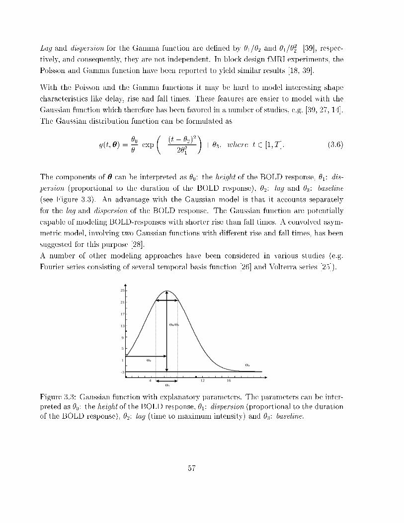
Lag and dispersion for the Gamma function are de�ned by �1=�2 and �1=�22 [39], respec-
tively, and consequently, they are not independent. In block design fMRI experiments, the
Poisson and Gamma function have been reported to yield similar results [18, 39].
With the Poisson and the Gamma functions it may be hard to model interesting shape
characteristics like delay, rise and fall times. These features are easier to model with the
Gaussian function which therefore has been favored in a number of studies, e.g. [39, 27, 14].
The Gaussian distribution function can be formulated as
g(t; �) =�0
�1exp
��(t� �2)
2
2�21
�+ �3; where t 2 [1; T ]: (3.6)
The components of � can be interpreted as �0: the height of the BOLD response, �1: dis-
persion (proportional to the duration of the BOLD response), �2: lag and �3: baseline
(see Figure 3.3). An advantage with the Gaussian model is that it accounts separately
for the lag and dispersion of the BOLD response. The Gaussian function are potentially
capable of modeling BOLD-responses with shorter rise than fall times. A convolved asym-
metric model, involving two Gaussian functions with di�erent rise and fall times, has been
suggested for this purpose [28].
A number of other modeling approaches have been considered in various studies (e.g.
Fourier series consisting of several temporal basis function [26] and Volterra series [25]).
��
��
��
��/��
-3
1
5
9
13
17
21
25
4 12 16
Figure 3.3: Gaussian function with explanatory parameters. The parameters can be inter-
preted as �0: the height of the BOLD response, �1: dispersion (proportional to the duration
of the BOLD response), �2: lag (time to maximum intensity) and �3: baseline.
57

Input
stimulus
Haemodynamic activity
-oxygen metabolism
- blood flow
- blood volume
Neuronal activity
- onset
- duration
BOLD
response
fMRI time
series
Figure 3.4: Physiological modeling of the BOLD-response in fMRI time series. The em-
phasis of physiological oriented models lie in the physiological mechanisms which leads
to the BOLD-response. The onset and duration of neuronal activity as well as oxygen
metabolism, blood ow and blood volume are features that a physiological model must
consider.
3.3 Physiological models
When using heuristic modeling functions such as the Gaussian function, we seek to asso-
ciate the parameters with physiological characteristics (such as lag and dispersion) related
to the BOLD-response. None of these function are, however, based on a comprehensive
physiological model. The sequence of events from the onset of neuronal activation to the
BOLD-response is complicated and only partly understood. Neuronal activity leads to
increased blood ow, which subsequently leads to changes in the magnetic properties of
blood. The signal is thus doubly indirect from the physiological factors of interest (i.e. the
synaptic activity of neurons). Furthermore, compared to the neuronal activity, the sig-
nal is delayed and dispersed in time. Physiologically oriented models emphasizes aspects
such as neuronal onset and duration times as well as oxygen delivery, blood volume and
dilatation/contraction of blood vessels etc. (see Figure 3.4).
It has been proposed that BOLD-responses are proportional to local average neuronal
activity over a short period of time. This should indicate that the relationship between
neuronal activity and the BOLD-response is completely characterized by a brief pulse of
neuronal activity. If this hypothesis was proven correct it would simplify the analysis
and interpretation of fMRI-data. However, experimental approaches testing this presumed
linearity of the BOLD-response have found that while it is approximately linear, there are
measurable nonlinear e�ects [14]. Despite this fact, this so called Linear Transform Model
is considered a reasonable approximation and several studies rely explicitly on the model
for their data analysis [18].
58

Stimulus Retinal V1
Pathway
fMRI Response
Noise
Haemo-dynamics
MRIScanner
Neuronal Response
Figure 3.5: fMRI Linear Transform Model (Modi�ed from Boynton et al., 1996). The output of
the retinal visual V1 pathway (i.e. neural response) varies non-linearly with visual stimulus
contrast. On the other hand, the fMRI signal mediated by the haemodynamics, is regarded
to be a linear transformation of neuronal activity such that the fMRI signal is proportional
to the neural activity averaged over a small spatial region and over a short period of time.
The individual noise processes a�ecting the fMRI response can be modeled as a single
additive noise source.
Within cognitive research it is desirable to separate neuronal and haemodynamic factors,
because this could lead to a better understanding of the neuronal mechanisms involved in a
cognitive task. The neuronal parameters should modulate characteristics such as neuronal
onset and duration, as well as amount of the neuronal activation. A number of approaches
can be taken in the modeling of the vascular parameters. However, in constructing a
physiological model, the number of parameters must be carefully considered. Since usually
just a limited number of time steps are recorded per trial, there is an upper bound for the
number of parameters.
The Convolved Compartment Model is based upon ow changes in body subspaces (com-
partments). The aim is to separate parameters describing the vascular component from
parameters describing the neuronal activation. To achieve this distinction the HRF is
viewed as a convolution between a neuronal activity function, n(�), and a physiologically
based haemodynamic function, f(�). The details of this model will be explored in Sec-
tion 5.3.
We will now give a brief description of the Balloon Model [9], in which a biomechanical
approach is considered. This model especially attempts to model the con icting e�ects of
the dynamic changes in blood oxygenation and (the relatively larger) blood volume.
At the onset of neuronal activity, both cerebral blood ow and the cerebral metabolic rate
59
of oxygen (CMRO2) increases. There is, however, a large gap between the cerebral blood
ow increase of 30 � 50% and the CMRO2 increase of approximately 5%. The Balloon
model is based on the premise that there is a strong coupling between blood ow and
oxygen metabolism, and that a small increase in CMRO2 must be supported by a large
increase in ow due to the biophysics of oxygen extraction. The model assumes that the
capillary volume remains �xed, but allows for an expansion in the venous part of the
vascular bed, hence the name Balloon model.
There is a close connection between the Balloon model and the Oxygen Limitation Model,
which assumes that increase in blood ow in the venous compartment is a result of increased
ow velocity on the capillary side.
An increase in the capillary transit time gives less time for di�usion and therefore a de-
crease in the amount of oxygen extracted from a particular blood volume. Increased blood
ow and thereby also increased blood volume leads, however, to a larger proportion of
oxyhaemoglobin on the venous part of the vascular bed and subsequently a stronger signal
(see Section 2.4.1). When neuronal activity decreases, the blood ow slows down thereby
reducing both venous blood volume and the relative amount of oxygen. This results in a
decreasing BOLD-response.
More speci�cally, for a vascular bed within a small volume of tissue of an expandable
compartment, Fin(t) denotes the volume ow into the compartment, and Fout(t) the volume
ow out of the compartment. An increase in Fin(t) causes the compartment to expand due
to intrinsic pressure in the compartment until a new steady state, where Fin equals Fout
is reached (see Figure 3.6). In reality Fout depends on factors such as pressure within
the compartment and resistance in the vessels following the compartment. For simplicity,
however, the Balloon model assumes that Fout merely is a function of the volume in the
compartment, Fout(V ).
The BOLD-response is calculated as a function of the venous blood volume and deoxy-
haemoglobin content. A detailed description of the Balloon Model is found in [9, 33].
60

arteriescapillaries
veins
vV
Fin(t) Fout(V)
Figure 3.6: Balloon Model. At the onset of neuronal activity, both cerebral blood ow and
the cerebral metabolic rate of oxygen (CMRO2) increases. The Balloon model hypotheses
that a small increase in CMRO2 must be supported by a large increase in ow and that
the capillary volume remains �xed, but allows for an expansion in the venous part of the
vascular bed. Fin(t) denotes the ow into the compartment, and Fout(t) the ow out of the
compartment. An increase in Fin(t) causes the compartment to expand due to intrinsic
pressure in the compartment until a new steady state, where Fin equals Fout is reached.
Fout is assumed to be a function of the volume in the compartment, Fout(V ). Modi�ed from
Buxton et. al
61
Chapter 4
Detection of the BOLD response in
fMRI
Measure what is measurable, and make measurable what is not so.
Galileo Galilei, quoted in I Gordon and S Sorkin, The Armchair Science Reader (New York 1959).
Most brain activation images relies on the concept that distinct regions "light up" during
particular tasks. These images illustrate the localization and degree of activation. To
produce such images, methods for detecting brain activation are required. This chapter
describes two signal detection models; ANOVA, which is a pure signal detection method
and Selective Averaging which also deals with overlapping BOLD-responses.
4.1 ANOVA [12]
Event-related experiments allows for the signal to be present in a small number of time
points, thereby enabling investigation of individual trials. Analysis of variance (ANOVA)
relies only on the timing of the start of each trial and thus makes no assumptions about the
temporal shape of the activation. This makes it possible to detect many di�erent activation
patterns. The main goal is to detect voxels in which the time course shows a repeatable
response to a particular type of stimuli. The haemodynamic response consists not only of
the genuine response to the stimuli in the activated voxels, but also of random uctuations
due to uncorrelated physiological events and noise in the images. Since noise in fMRI data
is assumed to have a normal distribution, averaging across trials reduces the magnitude of
the noisy component, but not that of the repeated signal (see Figure 4.1).
62

0
T (trial interval )
I IIII I I I III II II II II II II
2 trial types: I and II
Averaged time course for trial type I
T
Figure 4.1: Averaged responses in er-fMRI. Trial types I and II. Averaging is performed
over all trials of the same type. The magnitude of the noisy component is reduced, but
not that of the repeated signal (Modi�ed from R. Buckner, HBM 2000).
Description of method
An experiment may consist of one or several di�erent trial types, randomly intermixed.
The design should be such that each trial is presented after a suÆciently long interval to
allow the BOLD-response to return to baseline between trials. The data for each trial type
are collected and analyzed separately.
Let uij refer to the pixel intensity at the i-th time point after the stimulus and of the j-th
trial of an experiment with n trials and m time points in each single trial:
63

Trial
u11 u12 ::: u1j ::: u1n u1
u21 u22 ::: u2j ::: u2n u2
T ime ::: ::: ::: ::: ::: ::: :::
ui1 ui2 ::: uij ::: uin ui
::: ::: ::: ::: ::: ::: :::
um1 um2 ::: umj ::: umn um
u
The null hypothesis states that there are no signi�cant di�erences in the time point means,
ui. To test this hypothesis, two estimates of the time point means are compared, the �rst
based on variance between time points and the second based on variance within the same
time point.
Using standard statistical procedures, we begin by calculating the variance within the
same time point across all trials of the same type. The mean, ui and mean of means, u, is
calculated from
ui =1
n
nXj=1
uij ; u =1
m
mXi=1
ui ;
and the variance, s2u, of time point means is given by
s2u =
mXi=1
(ui � u)2
m� 1:
Let �̂2B denote mean variance between time points and �̂2W mean variance within time points.
Assuming
�2u =
�2B
n;
mean variance between time points, �̂2B, can be approximated by
�̂2B = n � s
2u = n �
mXi=1
(ui � u)2
(m� 1)
with (m� 1) degrees of freedom.
The variance within time points, s2i , is calculated from
s2i =
nXj=1
(uij � ui)2
n� 1; i = 1; :::; m
64
and mean variance within time points is thus given by
�̂2W =
mXi=1
nXj=1
(uij � ui)2
m(n� 1)
with m(n � 1) degrees of freedom. �̂2W is referred to as variance of the unaveraged data
set [13], or unexplained variance [44] because it represents random variations that cannot
be systematically explained. Accordingly, �̂2B is referred to as variance of the averaged data
set or explained variance.
The ratio F , which is the variance of the averaged data set to the variance of the unaveraged
data set, is calculated for each voxel in the image. The function
F =�̂2B
�̂2W
(4.1)
has a Fisher-distribution (see Appendix A.2) with (m�1) and m(n�1) degrees of freedom.
Any signal change that is time locked to the stimulus will result in a larger value of �̂2B than
expected under the null hypothesis. For voxels in regions with only random noise the ratio
will be around 1=n, where n is the number of trials averaged together. Voxels in regions
of activation will have a signi�cantly higher ratio due to the stimulus-locked change in the
BOLD-response.
P (probability) values are calculated for each voxel yielding a parametric statistical map
(SPM) where each voxel in the imaged volume is assigned a value on the likelihood that
the null hypothesis is false. By tresholding the SPM and highlighting areas of the brain
that can con�dently be labeled as active, localization and comparison of brain function can
be investigated.
65

4.2 Selective Averaging [14]
Averaging across trials is used to reduce noise in fMRI images. Dale and Buckner [14] have
explored whether averaging techniques similar to those applied in event-related potential
(ERP) experiments can be used to demonstrate BOLD responses to rapidly intermixed
trials. In these paradigms the trials are closely spaced and the haemodynamic responses
to adjacent trials may overlap distorting the averages for the selected trial type (selective
averaging). One could choose to present the trials suÆciently apart so that their responses
do not overlap. This will, however, reduce the total number of trials and thereby the power
of the test. A more attractive solution, illustrated in Figure 4.2, would be to present closely
spaced trials, and then apply methods for removing overlap. This requires a model for how
the measured haemodynamic response to a sequence of events relates to the response to
each individual event.
-1
0
1
2
3
4
-1
0
1
2
3
4
0 1 2 3 4 5 6 7 8 9 10 11 12 13 14 15 16 17 18 19
time(sec)
0 1 2 3 4 5 6 7 8 9 10 11 12 13 14 15 16 17 18 19
time(sec)
Trial 2
Trial 3
Trial 1
a b
Figure 4.2: Responses to three closely spaced trials. (a) the observed responses and (b)
the averaged responses
Description of method
The sampled fMRI time series are sorted by trial type after which the average and variance
of the fMRI time courses are estimated for each voxel. Let ti;k denote the start-time of the
66

kth trial of type i, and sti;k+j refer to the (ti;k + j)th sample of the signal. We can then
arrange the data from the ni trials of type i as follows :
Trials of type i
sti;1+1 sti;2+1 ::: sti;k+1 ::: yi;1
sti;1+2 sti;2+2 ::: sti;k+2 ::: yi;2
T ime ::: ::: ::: ::: ::: :::
sti;1+j sti;2+j ::: sti;k+j ::: yi;j
::: ::: ::: ::: ::: :::
The average BOLD response, yi;j, for trial type i at time j is computed by
yi;j =
Pnik sti;k+j
ni(4.2)
and the associated variance estimate �2i;j is
�2i;j =
Pnik (sti;k+j � yi;j)
2
ni � 1(4.3)
where ti;k is the start-time of the kth trial of type i, and sti;k+j refers to the (ti;k+j)
th sample
of the signal. The average, yi;j, and variance, �2i;j, are weighted by their corresponding
number of degrees of freedom (ni and (ni � 1), respectively). To arrive at a statistical
activation map, calculations of the covariance between the averaged observed signal and a
normalized predicted BOLD-response function is performed.
The predicted BOLD-response function is modeled with a Gaussian function:
g(t) =
�(t� Æ)
�
�2
e�(t�Æ)
� (4.4)
where Æ = 2:5 seconds and � = 1:25 seconds [14].
The average of the predicted response, g is calculated from
g =1
m
mXj=1
gj (4.5)
where gj denotes the predicted fMRI response at the j�th time point and m is the number
of time points in a single trial.
67

Similarly, the average of the observed signal, y, for a speci�c trial type i, is calculated from
y =1
m
mXj=1
yj (4.6)
where yj denotes the observed fMRI response at the j � th time point.
To obtain a good measure of how the observed signal relates to the predicted signal, the
correlation between them is computed. The correlation, q, given by
q =
Pmj (yj � y)(hj � h)qPm
j�2j
m
qPmj (hj � h)2
; (4.7)
is assumed be Student's t distributed with degrees of freedom equal to the number of
degrees of freedom for �2j [14].
68
Chapter 5
Description of the BOLD response in
fMRI
The models described so far have been aimed primarily at detecting the BOLD response and
the amount of this activation. They do not explore the shape properties (time course) of the
BOLD responses. Probing the secrets of cerebral activity requires, however, information
about both the spatial and the temporal properties of the BOLD response. In the process
of extracting the temporal properties of the BOLD-response, the modulation of the HRF
must be considered with great care. To avoid warped estimates of the true response, it is
desirable that the HRF-models should span the space of all viable responses.
In this chapter the focus will be on the estimation of haemodynamic parameters. For
simplicity, the locus of activation is assumed to be known, determined either from using
one of the models already described or a suitable software package (e.g. SPM99, see
Appendix A.3). The signal detection problem is thus separated from the signal description
problem.
The �rst two models, the Nonlinear Least Squares Model (Section 5.1) and the Kruggel
& Cramon Model (Section 5.2) apply a parametric modeling function for the HRF. They
also both obtain estimates on the model parameters in a weighted least squares approach.
However, because they di�er in the way they deal with noise, and for reasons of clarity
they are treated as separate models. Experiments with both these methods have been
performed and will be presented in Chapter 7. The last section describes the Convolved
Compartment Model in which a physiological modeling function is employed. Experiments
with this model is described in Chapter 7.
69

5.1 Nonlinear Least Squares Model
In this section a straight forward nonlinear regression model of the form
x(t) = g(t; �) + �(t); � � N(0; �) (5.1)
is explored. Here x(t) is the observed BOLD-response at time t, g(t; �) is the modeling
function with the parameter vector � = (�1; : : : ; �p) and �(t) is the stochastic part (zero
mean, Gaussian noise).
Any of the parametric modeling functions described in Section 3.2 can be used as the HRF
function, g(t; �), in Equation (5.1). For the HRF of this model we chose the Gaussian
function (Equation (3.6)). This choice is based on the simplicity of the Gaussian and the
ability to separately account for characteristics such as dispersion and lag, which might
re ect properties of neuronal activity. Averaging over all trials for each speci�c trial type
is performed for each voxel in a ROI time series. For an observed BOLD-response with m
trials and l time steps per trial we introduce the matrix X:
X =
266664
x11 x12 ::: ::: x1l
x21 x22 ::: ::: x2l
::: ::: ::: ::: :::
::: ::: ::: ::: :::
xm1 xm2 ::: ::: xml
377775
Since noise in fMRI time series can, at �rst approximation, be modeled as additive, inde-
pendent and identically distributed Gaussian, averaging over multiple trials will potentially
increase the Signal to Noise Ratio (SNR, see Section 2.2.8). The averaged BOLD-response
per voxel and per trial type, x = [x1; :::; xl], obtained by
xj =1
m
mXi=1
xij; j = 1; ::; l ;
is approximated by determining the parameters in the chosen HRF-model. One set of
parameter estimates is obtained for each voxel in all ROI time series and for each trial type.
This approach is potentially capable of displaying di�erences between di�erent activated
brain regions and di�erent trial types.
HRF-models where g(t; � is nonlinear with respect to the parameters, � = (�1; : : : ; �p), re-
quire a nonlinear estimation scheme. Using a least squares approach, the problem becomes
one of selecting the elements of � that minimizes the function
D(�) =
lXt=1
�xt � gt(�)
�t
�2
(5.2)
70

in which � denotes the variances of the residuals. Since noise is normally and identically
distributed, with �xed variance �t = �, the minimization problem in Equation (5.2) reduces
to :
D(�) =
lXt=1
(xt � gt(�))2 (5.3)
A brief outline of the solution to Equation (5.3) now follows [20]. Expanding D(�) around
the point �0 to a second order gives
D(�) = D(�0) + [rD(�0)] (� � �0) +1
2(� � �0)H (� � �0); (5.4)
where rD represents the gradient of the residual andH its second derivative (the Hessian).
Setting@D
@�=
@D(�)
@�+H(� � �0) = 0 (5.5)
gives the following iteration scheme for �nding the minimum
�new = �old �H�1 @D(�old)
@�(5.6)
To avoid computing second derivatives it is common practice to approximate H by JTJ
where J denotes the Jacobian matrix of partial derivatives. Substitution yields a new
formula:
�new = �old � [JT J]�1JT r (5.7)
in which r denotes the residuals between the observed signal and the HRF with estimated
values for �. This is the Gauss-Newton method for nonlinear least squares �tting.
71

5.2 Kruggel & Cramon Model [27]
The signal description problem will now be further investigated in the Kruggel & Cramon
Model [27]. This model di�ers from the Nonlinear Least Squares Model, presented in
the previous section, in the way it deals with noise. Rather than attempting to reduce
noise, by averaging over multiple trials, the noisy components are collectively modeled in
a covariance matrix. The Kruggel & Cramon Model also di�ers from the Nonlinear Least
Squares Model in that it estimates one parameter set for a cluster of voxels and for each
separate trial. These clusters are called regions of interest (ROI's) and usually contain 6-9
voxels in a 2-dimensional grid. For a region to qualify as a ROI for the Kruggel & Cramon
Model, certain membership criteria must be met. Two voxels are de�ned as �rst order
neighbours if they share a side. Second order neighbours share a corner. First and second
order neighbours are conventionally called 8-connected (see Figure 5.1).
�O�
OO
�O�
center voxel
2.order neighbour
1.order neighbour
Figure 5.1: Neighbourhoods. First order neighbours share a side and second order neigh-
bours share a corner.
Voxels that are to be de�ned within a ROI must be 8-connected and, furthermore, before
a region is de�ned as a ROI, similarity measures (usually involving mean signal intensity
level) must be investigated. On the basis of these similarity criteria, suitable voxels can be
merged into a ROI. In the following a ROI denotes a set of voxels within one trial interval
and a ROI time series refers to a set of voxels over a sequence of trials. A description of
the Kruggel & Cramon Model now follows below.
72
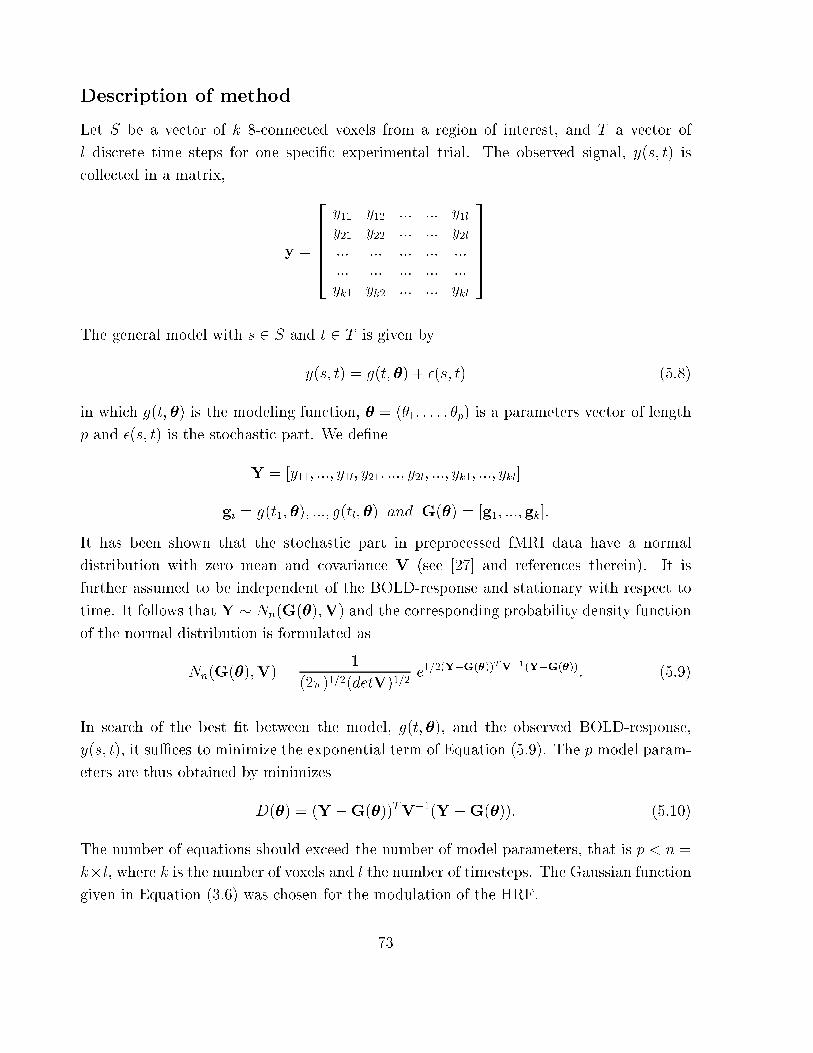
Description of method
Let S be a vector of k 8-connected voxels from a region of interest, and T a vector of
l discrete time steps for one speci�c experimental trial. The observed signal, y(s; t) is
collected in a matrix,
y =
266664
y11 y12 ::: ::: y1l
y21 y22 ::: ::: y2l
::: ::: ::: ::: :::
::: ::: ::: ::: :::
yk1 yk2 ::: ::: ykl
377775
The general model with s 2 S and t 2 T is given by
y(s; t) = g(t; �) + �(s; t) (5.8)
in which g(t; �) is the modeling function, � = (�1; : : : ; �p) is a parameters vector of length
p and �(s; t) is the stochastic part. We de�ne
Y = [y11; :::; y1l; y21; :::; y2l; :::; yk1; :::; ykl]
gi = g(t1; �); :::; g(tl; �) and G(�) = [g1; :::; gk]:
It has been shown that the stochastic part in preprocessed fMRI data have a normal
distribution with zero mean and covariance V (see [27] and references therein). It is
further assumed to be independent of the BOLD-response and stationary with respect to
time. It follows that Y � Nn(G(�);V) and the corresponding probability density function
of the normal distribution is formulated as
Nn(G(�);V) =1
(2�)1=2(detV)1=2e1=2(Y�G(�))TV�1(Y�G(�))
: (5.9)
In search of the best �t between the model, g(t; �), and the observed BOLD-response,
y(s; t), it suÆces to minimize the exponential term of Equation (5.9). The p model param-
eters are thus obtained by minimizes
D(�) = (Y �G(�))TV�1(Y �G(�)): (5.10)
The number of equations should exceed the number of model parameters, that is p < n =
k�l, where k is the number of voxels and l the number of timesteps. The Gaussian function
given in Equation (3.6) was chosen for the modulation of the HRF.
73

Studies of the covariance structure in fMRI data (see [27] and references therein) have found
that the BOLD-response, y(s; t), is autoregressive, that is, it depends on the external input
stimuli and y(s; t� 1). For a weakly stationary process the correlation between residuals
�(s0; t0) and �(s1; t1) depend only on the distance between them in time and space. Hence,
the correlation matrix V is de�ned by the variance of the residuals ( 22) and the lag � 1
autocorrelation in the x,y and t directions. For the estimation scheme in Equation (5.10)
it is required that V has an inverse, and consequently, V must be nonsingular. The corre-
lation coeÆcients are estimated separately in time and space, yielding a spatial correlation
matrix, VS, and a temporal correlation matrix, VT . V�1 is given by
V�1 =1
22
(V�1S �V�1
T ) (5.11)
in which � denotes the Kronecker product1.
The temporal lag � 1 autocorrelation coeÆcient is computed from the formula :
�̂T =
Ps2S
�Pl�1t=1 �(s; t) �(s; t� 1)
�P
s2S
�Pl�1t=0 �(s; t)
2
� (5.12)
and the temporal correlation matrix is set up
V�1T =
1
(1� �2T )
0BBBB@
1 ��T 0 ::: 0
��T 1 + �2T ��T ::: 0
0 ��T 1 + �2T ::: 0
:::
0 ::: 1
1CCCCA (5.13)
To �nd the spatial correlation matrix is more involved. Here we closely follow the paper
of Kruggel & Cramon with references to [40]. First, the subsets of all pairs of sites located
with the same absolute distance are collected, that is :
Sh;v = f(si; sj) j si; sj 2 Sg
where h = H(si; sj); v = V (si; sj) returns the absolute distance in the x and y directions.
The correlation coeÆcients for all possible combinations of h and v are then computed:
�̂h;v =
Pt2T
�Psi;sj2Sh;v
�(si; t) �(sj; t� 1)�
Pt2T
�Psi;sj2Sh;v
�(si; t)2� (5.14)
1The Kronecker product of the two matrices S and T is the k2� l2 matrix V obtained by replacing the
entry sij of S with the matrix sijT
74

The correlation coeÆcients, �X and �Y , are found by minimizing
Xh;v
(�̂h;v � �hX �
vY )
2; (5.15)
after which the spatial correlation matrix is set up as
VS =
0BBBB@
1 �S(s0; s1) �S(s0; s2) ::: �S(s0; sk�1)
�S(s0; s1) 1 �S(s1; s2) ::: �S(s1; sk�1)
�S(s0; s2) �S(s1; s2) 1 ::: �S(s2; sk�1)
::: ::: ::: ::: :::
�S(s0; sk�1) ::: ::: ::: 1
1CCCCA (5.16)
in which
�S(si; sj) = �hX �
vY :
Optimization
When the covariance matrix has been set up, the next step is to minimize D(�) in Equa-
tion (5.10). Optimization is the process in which the "best" parameters for the function
D : Rn! R are chosen. These parameters are often found where D takes on a minimum
or a maximum, commonly referred to as an extreme point. An extreme point may be either
global or local. Ideally, the optimization method should converge to the optimal solution,
and not get caught in a local minima or maxima. Optimization methods can be divided
into two main categories; gradient methods, in which an approximation of the function's
derivative is required, and direct search methods where no derivatives are necessary.
Kruggel & Cramon suggests the Nelder & Mead downhill simplex method for the opti-
mization of the present model [27]. Nelder& Mead downhill simplex method is a direct
search method. A simplex is a geometrical �gure that has one more vertex that dimension;
a triangle in 2D, a tetrahedron in 3D, and so on. An initial simplex is formed by picking
a random location and taking unit vectors for the edges. The function being minimized
is then evaluated at the D+1 vertices of the simplex. An iterative procedure will at each
step attempt to improve the position of the "worst" vertex. During this process the worst
vertex is moved to a new location via a series of update moves (re ection, re ection and
expansion, contraction, multiple contraction, see Figure 5.2). If the move results in a
better position, the vertex position is updated. The procedure continues until a stopping
criteria is reached. A detailed description of the method can be found in [20]. Direct
search methods are usually preferable if derivatives cannot be accurately computed and
75

reflect
Highest point
SIMPLEX
mean
contract towards minimum
Reflect and expansion Reflect and contract
multiple contraction
Figure 5.2: Downhill simplex update moves
numerical approximations of derivatives are expensive and the values of D are noisy, which
is the case for fMRI-data. The Gaussian function (Equation 3.6) has only four parameters
and numerical approximation of the derivatives are readily computed. Furthermore, the
Kruggel & Cramon Model presents a way of dealing with noise. It is therefore relevant to
explore whether gradient based methods may be employed for the parameter estimation
of this model. The Levenberg-Marquardt method, as implemented in the Matlab function
lsqnonlin (see Appendix A.4), was chosen for this purpose.
The Gauss-Newton method (described in Section 5.1) converges quickly close to a mini-
mum, it is, however, extremely unreliable far from a minimum. The Levenberg-Marquardt
(LM) algorithm solves this problem by switching between gradient descent, which takes a
step in the direction in which the error is decreasing most rapidly far away, and Gauss-
Newton near a minimum. LM modi�cation adds � I to JT J in Equation (5.7), adjusting
the parameter � continuously :
�new = �old � [JT J+ � I]�1JT r: (5.17)
For � = 0 the algorithm is pure Gauss-Newton, but as �!1 the algorithm descends by
use of the gradient and thus becomes the method of gradient descent. If a step reduces
the error then � is decreased because Gauss-Newton is best close to a minimum. If, on
the other hand, a step increases the error then � is increased since gradient descent is
76

better. However, special attention regarding starting conditions are necessary. Whereas
the function to minimize may possess many minima, the Levenberg-Marquardt method will
only �nd the local minima closest to the starting conditions. The Levenberg-Marquardt
method therefore requires a starting value near the desired minimum, as well as a relative
smooth function.
77

5.3 Convolved Compartment Model [28]
The BOLD-response is interpreted as a convolution between neuronal activation and haemo-
dynamics, and a major problem with fMRI data is that they re ect changes in the Blood
Oxygenation Level, and not the desired neuronal activation. The question arises as to
what extent it is possible to distinguish the "neuronal" from the "vascular" component. A
deconvolution of the BOLD-response could prove useful in the search for the characteristics
of neuronal activation. A method which attempt to model this convolution process will
now be presented.
Description of method
To accommodate the convolution between neuronal activity and haemodynamics, Equa-
tion (3.3) is reformulated as
y(s; t) = f(t) ? n(t) + b + �(s; t) (5.18)
where y(s; t) is the observed signal intensity at site s and time t, n(t) denotes a neuronal
stimulation function, f(t) the haemodynamic modulation function, b is a baseline term
and ? is the convolution operator (cfr. Appendix A.1). If we include the parameter vector
� = [a; t0; t1; b; 0; 1; 2; 3], Equation (5.18) can be written
y(s; t; a; t0; t1; b; 0; 1; 2; 3) = f(t; 0; 1; 2; 3) ? n(t; a; t0; t1) + b + �(s; t): (5.19)
The neuronal stimulation function is modeled as a simple box-wave function:
n(t) =
�a if t0 � t < t0 + t1
0 otherwise(5.20)
This gives three neuronal parameters, a: gain of neuronal response, t0: time of onset and t1:
duration of neuronal response. In search of the vascular parameters, the BOLD response is
thought of as an endogenous contrast. Exogenous contrast such as radioactive markers or
pharmaceuticals have been modeled by compartment models since 1920 (see [28] and refer-
ences therein). Compartments refer to body subspaces such as tissue or vasculature. Taking
advantage of this modeling approach, and assuming that the measured BOLD-response is
proportional to the oxyhaemoglobin concentration, a compartment model should re ect
the temporal oxygen ow pattern. Increasing the proportion of oxyhaemoglobin leads to
decreased spin-spin dephasing and thereby a stronger signal (see Section 2.4.1). Thus, if
the concentration of oxyhaemoglobin in a compartment increases, so will also the signal
contribution from the particular compartment.
78

(f1) Arterial Compartment
(f2) Capillary Compartment
(f3) Tissue Compartment
Venous Compartment
�� ��
��
��
Figure 5.3: Movement of oxygen in vascular and tissue compartments. 0 denotes the
rate at which oxyhaemoglobin enters the capillary compartment. Rates 1 and 2 re ect
the oxyhaemoglobin exchange between capillaries and tissue, and 3 is the rate at which
oxyhaemoglobin ows into the venous system. Modi�ed from Kruggel & Cramon[1999]
The Convolved Compartment Model consists of two vascular and one tissue compartment.
The signal contribution from the venous side of the vascular bed is ignored. An illus-
tration of the model is given in Figure 5.3. Oxyhaemoglobin is transported from the
arterial compartment into the capillary compartment at rate 0. Rates 1 and 2 re ect
the oxyhaemoglobin exchange between capillaries and tissue, and 3 is the rate at which
oxyhaemoglobin ows into the venous system.
The model is described by the following linear system of di�erential equations2:
df1
dt= � 0f1; f1(0) = 1
df2
dt= 0f1 + 2f3 � ( 1 + 3)f2; f2(0) = 0
df3
dt= 1f2 � 2f3; f3(0) = 0
The solution to this system can be written as a sum of exponentials for the i � th com-
partment:
fi = ki1e� 0t + ki2e
�0t + ki3e�1t; (5.21)
2A misprint in the last equation of this system, reading�
f3= 0f2 � 2f3, was found in the paper [28].
79

in which the eigenvalues �0 and �1 are given by:
�0 = �0:5( 1 + 2 + 3 +p( 1 + 2 + 3)2 � 4 2 3);
�1 = �0:5( 1 + 2 + 3 �p( 1 + 2 + 3)2 � 4 2 3)
and the ki;j's are3:
k1;j = [1; 0; 0];
k2;j =
� 0( 2 � 0)
( 0 + �0)( 0 + �1);
0( 2 + �0)
( 0 + �0)(�0 � �1);
0( 2 + �1)
( 0 + �1)(�1 � �0)
�
k3;j =
� 0 1
( 0 + �0)( 0 + �1);
0 1
( 0 + �0)(�0 � �1);
0 1
( 0 + �1)(�1 � �0)
�
The parameter vector, �, now consist of eight parameters: [a; t0; t1; b; 0; 1; 2; 3], in which
a, t0 and t1 are neuronal parameters, 1� 4 are vascular transfer rates and b is the baseline.
The convolution between the neuronal and vascular components g(t; �) = f(t) ? n(t); is
de�ned as the de�nite integral:
g(T ) =
Z T
0
f(t)n(T � t)dt; f; n; t 2 [0; T ] 7! R (5.22)
in which the integral [0; T ] corresponds to the time interval of one single trial. Based on
Equation (5.20) and (5.22), g(T ) has the following properties:
g(T ) =
8>>>>><>>>>>:
0 0 � T < t0
aR T�t00
f(t)dt t0 � T < t0 + t1
aR T�t0T�t0�t1
f(t)dt T � t0 + t1
(5.23)
where f(t) = f1(t) + f2(t) + f3(t). Integrating Equation (5.23) with regard to t yields :
Z T�t0
0
f(t)dt = �
Pki;1
0
�e� 0(T�t0) � 1
�+
Pki;2
�0
�e�0(T�t0) � 1
�+
Pki;3
�1
�e�1(T�t0) � 1
�
and
3In the paper [28] the denominator for the k3;j are 0 1( 2 � 0), 0 1( 2 + �0) and 0 1( 2 + �1),
respectively. We assume that this is a misprint.
80
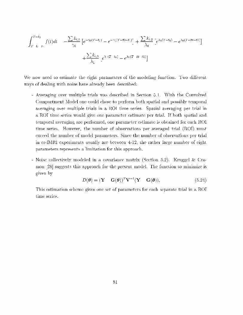
Z T�t0
T�t0�t1
f(t)dt = �
Pki;1
0
�e� 0(T�t0) � e
� 0(T�t0�t1)�+
Pki;2
�0
�e�0(T�t0) � e
�0(T�t0�t1)�
+
Pki;3
�1
�e�1(T�t0) � e
�1(T�t0�t1)�
We now need to estimate the eight parameters of the modeling function. Two di�erent
ways of dealing with noise have already been described:
- Averaging over multiple trials was described in Section 5.1. With the Convolved
Compartment Model one could chose to perform both spatial and possibly temporal
averaging over multiple trials in a ROI time series. Spatial averaging per trial in
a ROI time series would give one parameter estimate per trial. If both spatial and
temporal averaging are performed, one parameter estimate is obtained for each ROI
time series. However, the number of observations per averaged trial (ROI) must
exceed the number of model parameters. Since the number of observations per trial
in er-fMRI experiments usually are between 4-12, the rather large number of eight
parameters represents a limitation for this approach.
- Noise collectively modeled in a covariance matrix (Section 5.2). Kruggel & Cra-
mon [28] suggests this approach for the present model. The function to minimize is
given by
D(�) = (Y �G(�))TV�1(Y �G(�)); (5.24)
This estimation scheme gives one set of parameters for each separate trial in a ROI
time series.
81

82

Part III
Experiments
83

84

Chapter 6
Applied Methods and
Implementations
This chapter focuses on the speci�c implementation of methods described in Chapter 4
and 5. The models selected for experimental purposes of this work are as follows:
� Signal detection : ANOVA (Section 4.1)
� Signal description
- Nonlinear Least Squares Model (Section 5.1)
- Kruggel & Cramon Model (Section 5.2)
- Convolved Compartment Model (Section 5.3)
All programs are implemented in Matlab (www.mathworks.com). Matlab, which is avail-
able on a number of platforms including Windows 95/98/2000, Macintosh, several Unix
platforms and Linux, is especially suitable for matrix handling. Several toolboxes are
available, including toolboxes for signal and image processing and statistical analysis. A
number of Matlab functions have been included in the implementation of the models and
will be referred to in the appropriate sections.
All data sets employed in this thesis have been preprocessed with the SPM99 software
package (see Appendix A.3). Before proceeding with a detailed description of the selected
models, a brief description of the SPM preprocessing procedure will therefore be given.
6.1 Preprocessing with SPM99
SPM99 is a software environment for the analysis of PET (Positron Emission computed
Tomography) and fMRI neuro-imaging data. The software package contains functionalities
85
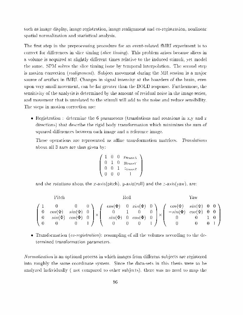
such as image display, image registration, image realignment and co-registration, nonlinear
spatial normalization and statistical analysis.
The �rst step in the preprocessing procedure for an event-related fMRI experiment is to
correct for di�erences in slice timing (slice timing). This problem arises because slices in
a volume is acquired at slightly di�erent times relative to the induced stimuli, yet model
the same. SPM solves the slice timing issue by temporal interpolation. The second step
is motion correction (realignment). Subject movement during the MR session is a major
source of artifact in fMRI. Changes in signal intensity at the boarders of the brain, even
upon very small movement, can be far greater than the BOLD response. Furthermore, the
sensitivity of the analysis is determined by the amount of residual noise in the image series,
and movement that is unrelated to the stimuli will add to the noise and reduce sensibility.
The steps in motion correction are:
� Registration : determine the 6 parameters (translations and rotations in x,y and z
directions) that describe the rigid body transformation which minimizes the sum of
squared di�erences between each image and a reference image.
These operations are represented as aÆne transformation matrices. Translations
about all 3 axes are thus given by:
0BB@
1 0 0 xtransX
0 1 0 ytransY
0 0 1 ztransZ
0 0 0 1
1CCA
and the rotations about the x-axis(pitch), y-axis(roll) and the z-axis(yaw), are:
Pitch Roll Yaw0BB@
1 0 0 0
0 cos(�) sin(�) 0
0 �sin(�) cos(�) 0
0 0 0 1
1CCA�
0BB@
cos(�) 0 sin(�) 0
0 1 0 0
�sin(�) 0 cos(�) 0
0 0 0 1
1CCA�
0BB@
cos(�) sin(�) 0 0
�sin(�) cos(�) 0 0
0 0 1 0
0 0 0 1
1CCA
� Transformation (co-registration): resampling of all the volumes according to the de-
termined transformation parameters.
Normalization is an optional process in which images from di�erent subjects are registered
into roughly the same coordinate system. Since the data-sets in this thesis were to be
analyzed individually ( not compared to other subjects), there was no need to map the
86

images to a standard template. The normalization step was therefore omitted. Finally,
the images are smoothed. Smoothing, which in SPM is a convolution between the sampled
image and a Gaussian kernel, is performed to increase the Signal to Noise Ratio (SNR, see
Section 2.2.8).
REALIGNMENT SMOOTHING
NORMALISATION
DATA ANALYSIS
fMRI TIME-SERIES Kernel
SLICE TIMING
Figure 6.1: SPM preprocessing process. The fMRI time series is �rst subject to slice-timing
in which data are corrected for the di�erence in the image acquisition times between slices.
Realignment seeks to reduce noise (i.e. misregistration) related to movement. All volumes
of the fMRI time series are aligned according to the �rst volume. This involves a spatial
transformation to minimize the di�erence between two volumes. Normalization is the pro-
cess of registering images from di�erent subjects into roughly the same coordinate system.
Smoothing, a low pass �ltering in which the images are convolved with a kernel shaped
according to the applied �lter, is performed to to increase the SNR (see Section 2.2.8)
As an example of SPM analysis in terms of detection of activated voxels, a recent experi-
mental study on dichotic listening (see below) was selected. We used a gradiant echo, EPI
protocol, echo time TE = 60 msec, TR = 0.6 msec and ip angle = 90Æ (FOV = 220�220
mm), and a total of 472 echo planar images (EPI, see Section 2.2.7) were acquired. Each
volume consisted of 9 slices of 64 �64 voxel resolution and spatial resolution 3.44�3.44�5
87

mm, no gap between consecutive slices. A corresponding anatomical image (3D FLASH,
see Section 2.2.7) was acquired in the same session.
While in the scanner, the subject was presented with dichotic listening tasks in which
similar sounds (e.g ba, pa) is presented to both ears simultaneously. These sounds were
also presented to the subject on a visual display. The subject was asked to determine
which of the sounds he had heard. Presentation rate was a �xed interval of 21 seconds.
The data set was preprocessed and analyzed with the SPM software package. Expected
areas of activation include primary and secondary auditory cortex (see Figure 6.2). The
activation map constructed with SPM is shown in Figure 6.3.
A general problem with auditory stimulus in fMRI experiments is that the level of back-
ground noise in the scanner is extremely high. This presumably leads to a constant acti-
vation in the auditory cortex. Over time, however, there will be a certain adaptation to
the scanner noise which also has speci�c frequency characteristics. It should therefore in
theory be possible to detect the activation that arises from the very brief auditory stimulus
applied in this experiment.
88

Lateral fissure
Primary auditorycortex
Secondary auditorycortex
Figure 6.2: Auditory cortex
Figure 6.3: SPM activation map. SPM analysis in terms of detecting activated voxels in a
dichotic listening study.
89

6.2 ANOVA
The ANOVA procedure is based on simple averaging theory (see [13] and references therein)
and implementation is straightforward. A formal description of the method is given in
Chapter 4.1. The ANOVA approach assumes that each time point is independent and the
experimental design must therefore allow for the response to return to baseline between
successive trials. If the duration of the BOLD-response is longer than the trial sampling
period, the time points no longer can be considered independent. However, if the data have
a high level of temporal connectivity, it has been suggested that a method of randomization
be applied [13]. In short this means that the order of the time series for each separate trial
is randomized prior to the processing and statistical analysis.
The F-ratio, given in Equation (4.1), di�ers with varying degrees of freedom in numerator
and denominator (see Appendix A.2). For the current problem, the degree of freedom for
the numerator is the number of time points minus one. For the denominator, the degrees
of freedom is given by the total number of observations (number of trials � number of time
points) minus the number of time points per trial [44].
To assess the validity of ANOVA with fMRI noise levels, the procedure was tested on
real data. The data set, consisting of 45 volumes, each of 64 � 64 � 40 matrix size, was
analyzed with the SPM software package after which regions with activated voxels were
excluded from further tests. All remaining voxel time series were submitted to the ANOVA
procedure after which the resultant F-values were investigated. All test showed a good �t to
the F-distribution, con�rming the validity of the technique on fMRI data. An illustration
is given in Figure 6.4.
The data should be organized such that all time points and all trials for each trial type
are collected in a separate matrix. This m� n matrix, in which m is the number of time
points in each trial and n is the number of trials, is taken as input to the Matlab m-�le,
ihk ANOVA. Pseudo code for the algorithm follows below.
Pseudo code ihk ANOVA :
INPUT:
� data ( [m�n] data matrix where m is the number of time points in each trial and n is thenumber of trials)
OUTPUT:
� F (F-ratio)
90
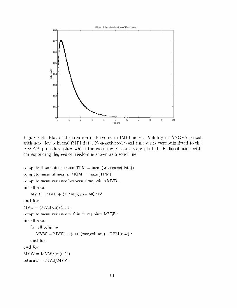
0 1 2 3 4 5 6 7 8 9 100
0.1
0.2
0.3
0.4
0.5
0.6
0.7
0.8Plots of the distribution of F−scores
F−score
arb.
uni
ts
Figure 6.4: Plot of distribution of F-scores in fMRI noise. Validity of ANOVA tested
with noise levels in real fMRI data. Non-activated voxel time series were submitted to the
ANOVA procedure after which the resulting F-scores were plotted. F distribution with
corresponding degrees of freedom is shown as a solid line.
compute time point means: TPM = mean(transpose(data))
compute mean of means: MOM = mean(TPM)
compute mean variance between time points MVB :
for all rows
MVB = MVB + (TPM(row) - MOM)2
end for
MVB = (MVB�n)/(m-1)
compute mean variance within time points MVW :
for all rows
for all columns
MVW = MVW + (data(row,column) - TPM(row))2
end for
end for
MVW = MVW/(m(n-1))
return F = MVB/MVW
91

6.3 Nonlinear Least Squares Model
The Nonlinear Least Squares approach is the least complex of the signal description mod-
els presented in this work. A general overview of this method is found in Chapter 5.1. In
this section a more detailed description is presented. The Nonlinear Least Squares Model
ignores all spatial and/or temporal correlations present in the noise. Therefore, it is im-
portant that the noisy component is reduced. This is achieved by performing an averaging
over all trials of the same type (Single Trial Averaging) for each voxel. In order to reduce
the noise to an acceptable level, a large number of trials are required for all trial types.
In Single Trial Averaging the mean over all trials is computed for every voxel yielding one
parameter (vector) estimate for each speci�c trial type. Given m trials per trial type and
l time steps per trial, the averaged BOLD-response, x = [x1; :::; xl], per voxel is given by
xj =1
m
mXi=1
xij; j = 1; ::; l ;
This approach is valid only under the assumption that identical trial types generate the
same response in a speci�c voxel. To avoid adaptation to the imposed external stimulus it
is required that the experiment is event-related with randomly intermixed trial types.
A Gaussian form was selected for the parametric modeling function. The Gaussian mod-
eling function
g(t; �) =�0
�1exp
��(t� �2)
2
2�21
�+ �3; where t 2 T; (6.1)
has been preferred in many studies because of its ease of application and its ability to
independently represent lag and dispersion [39]. In a physiological interpretation of the
parameters lag (�2) can be understood as the time to maximum of the BOLD-response,
whilst dispersion (�1) re ects the duration of the response. Gain (�0) has been proposed
to re ect the energy consumption of an activated area and (�3) the baseline [39].
For the minimization of D(�) in Equation (5.3), the Gauss-Newton method for nonlinear
least squares �tting was employed. This procedure is implemented in nlinfit (see Ap-
pendix A.4). To test the validity of nlinfit with the Gaussian function (Equation (6.1)),
various signals with known true parameters were constructed. Given these signals, nlinfit
should be able to reproduce the true parameters. A slight modi�cation of nlinfit, chang-
ing the convergence criteria from 10�4 to 10�12, ensured an acceptable �t. The modi�ed
version, ihk nlinfit yields parameter estimates that are identical with the true param-
eters with at least 14 decimals. The Matlab function nlparci (see Appendix A.4) was
92

��(dispersion)
[��, ��, �� , ��]= [98.0, 3.5, 6.5,-3.0]
��(lag)��(baseline)
��/��
��/�� : the quotient of gain and dispersion reflects the height of the
response
-3
1
5
9
13
17
21
25
4 12 16
Figure 6.5: Gaussian function with physiological interpretations of the parameters:(�0) is
assumed to re ect the energy consumption of an activated area, (�1) the duration of the
response, (�2) the time to maximum of the BOLD-response and (�3) is the baseline.
employed for the computation of 95% con�dence intervals on the p model parameters,
� = (�1; : : : ; �p). Normality in the residuals for all ROI's were tested according to the
Lilliefors and the Bera-Jarque tests implemented in the Matlab functions lillietest and
jbtest, respectively (see Appendix A.4).
A brief outline of the MATLAB code follows below:
Matlab function ihk lsq :
INPUT:
� ROI (matrix of data points in which rows represents voxels and columns represents timepoints. There are l time points in each trial. Consecutive trials must be such that the lasttime point in one trial is directly followed by the �rst time point in the next trial)
� t (vector with time interval for one trial, if e.g. t = [0 : 2 : 22] then there are 12 time pointsand 2 seconds between each time point)
� start (starting values for the parameter vector)
OUTPUT:
� theta est (vector with estimated parameters)
� conf int (95% con�dence interval for the parameter vector, theta est)
� h tab (table of results from Lilliefors and Bera-Jarque tests for normality in the residuals)
93

theta est = [ ]; % matrix for estimated parameters
h tab = [ ];l=length(t)[k; n] = size(ROI); % k voxels and n time points, n =l� number of trials
%Single Trial Averaging: compute mean over all trials
mean ROI = [ ];for voxel = 1:k
ROI voxel = [ ];for trial = 1:l:n
if trial + (l-1) � n
ROI voxel = [ROI voxel; ROI(voxel,trial:(trial+(l-1)))];end if
end for
%compute the average over all timepoints
mean ROI(voxel,:) = mean(ROI voxel);end for
% nonlinear least-squares data �tting by the Gauss-Newton method
model = 'gaussmodelHR'; % Subroutine for use with ihk nlin�t
res after est = [ ]; % matrix for residuals after estimation
conf upper = [ ]; conf lower = [ ];for voxel = 1 : k
[thetahat, resid, J] = ihk nlin�t(t,mean ROI(voxel,:), model, start);betaci = nlparci(thetahat, resid, J);conf lower = [conf lower; transpose(betaci(:,1))];conf upper = [conf upper; transpose(betaci(:,2))];theta est(voxel,:) = transpose(thetahat);res after est(voxel,:) = transpose(resid);
end for
conf int= (conf upper-conf lower)/2;
% Test for normality in the residuals
for voxel = 1:k
% Lilliefors test for goodness of �t to a normal distribution
H = lillietest(res after est(voxel,:), 0.01);
h tab(voxel,1) = H;
% Bera-Jarque test for normality in the residuals
H = jbtest(res after est(voxel,:), 0.01);
h tab(voxel,2) = H;
end for
return;
94
6.4 Kruggel & Cramon Model
This section considers the details of implementation for the Kruggel & Cramon Model.
The general model description is found in Section 5.2. This model di�ers from the previous
model in the way it deals with noise. Temporal and/or spatial correlations in the residuals
are applied as weights in a weighted least squares approach. One set of parameters is then
estimated for each separate trial in a ROI time series.
The estimation procedure, in which one set of parameters is estimated for each trial (ROI),
was implemented in a matlab m-�le, ihk kruggel. This function calls several other m-�les
for the calculation of the covariance structure and parametric modeling function. The
parametric modeling function is the Gaussian function as described by Equation (6.1) and
illustrated in Figure 6.5. Two approaches were investigated for the minimization of
D(�) = (Y �G(�))TV�1(Y �G(�)) (6.2)
1. Levenberg-Marquardt method, as implemented in the Matlab function lsqnonlin
(see Appendix A.4), and
2. multi-dimensional unconstrained nonlinear minimization by Nelder-Mead Downhill
SimplexMethod as implemented in the Matlab function fminsearch (see Appendix A.4).
lsqnonlin does not take the covariance matrix, V�1, as input argument. An adjustment
of the object function (Equation (6.2)) is therefore necessary. V�1 is both symmetric and
positive de�nit1. Choleskys factorization can therefore be applied, producing an upper
triangular matrix, L, such that V�1 = LTL. Substitution yields
D(�) = (L(Y �G(�)))T (L(Y �G(�)));
which is valid input for lsqnonlin.
Before employing the estimation methods, however, tests concerning their ability to re-
produce the true parameters were performed. For this purpose, signals with known true
parameters were constructed from the Gaussian modeling function. Both lsqnonlin and
fminsearch achieve a good �t when starting values are relatively near the true parameters.
By appropriately setting the tolerance, lsqnonlin succeeded in �nding the true parameters
even with extremely bad parameter starting values. fminsearch fails, however, to arrive
at the true values if the initial parameter values are far from the true values. Fortunately,
1Positive de�nit: An n n�n matrix, M , is positive de�nit if for every n component vector, xTMx � 0,
furthermore xTMx = 0 only if x is the zero vector. Equivalent de�nition: M has all positive eigenvalues.
95
the intervals for realistic starting values are not too diÆcult to �nd (e.g. the parameter
lag should be given a starting value according to the expected time to maximum of the
BOLD-response, usually between 2 and 6 seconds), and fminsearch performs acceptably
within these limits. The use of fminsearch is therefore justi�ed.
The procedure was implemented in Matlab and the core functions follow below. For simplic-
ity, the code is shown only with lsqnonlin for the optimization of D(�) in Equation (6.2).
ROI's consisting of k voxels in l 2-dimensional grids are reorganized into matrices ROI(s,t)
such that s = 1; ::; k; and t = 1; ::; l. In this work all ROI's are 3 � 3 voxel grids (i.e k = 9).
The function ihk Kruggel accepts a k� l matrix (ROI) as input. Choleskys factorization
and calculation of the Kronecker product is performed by the Matlab routines chol and
kron. The Matlab function nlparci is employed for the computation of 95% con�dence
intervals on the model parameters, �, and normality in the residuals is explored using
the Matlab functions lillietest and jbtest. For a brief outline of the employed Matlab
functions see Appendix A.4. Code for the subroutines ihk argmin, ihk gaussmodelHR and
ihk find rhoxy are not shown. ihk argmin is used with lsqnonlin and returns a scalar
value, res=L� (Y�G), ihk gaussmodelHR returns a vector g = g1; :::; gl representing the
Gaussian modeling function and ihk find rhoxy is used with ihk nlinfit and returns a
vector, result = �hX �vY for all combinations of h and v.
96

Matlab function ihk kruggel :
INPUT :
� ROI (matrix with k rows (voxels) and l columns (time points in a single trial))
� t (vector with time points, if t = [0 : 2 : 22] then the trial has 12 time points with 2 secondinterval between each time point)
� start (starting values for the model parameter vector (theta))
� N (number of desired iterations to compute the spatiotemporal correlation matrix (andoptimize D(�) in Equation (6.2)))
� tolx (termination tolerance on model parameter vector (theta))
� tolfun (termination tolerance on the function value)
OUTPUT:
� est theta (vector of estimated model parameters)
� betaci (95% con�dence interval for the model parameter vector, theta est)
� h tab (table of results from Lilliefors and Bera-Jarque tests for normality in the residuals)
[k; l] = size(ROI); % k voxels and l time points
x = [1,1]; % starting values for �X and �Y
model = ihk argmin; % subroutine for use with lsqnonlin
Y = reshape(transpose(ROI), 1, k*l);theta = start;
for rep = 1 : N% compute the gaussian modeling function with current values of theta
g = ink gaussmodelHR(theta,t) ;
% �nd the residuals
for i = 1: kresidual(i,:) = ROI(i,:) - g ;
end for
% compute V inv from the residuals
gamma2 = var(var(transpose(residual)));rhoT = ihk compute rhoT(residual);V inv time = ihk setup V inv time(rhoT,l);V inv = ihk inverseV(residual, gamma2, V inv time, x);
L = chol(V inv); % Cholesky factorization V inv = transpose(L)*L
opt = optimset('LargeScale','o�','MaxFunEvals', 1000,'TolX',tolx,'TolFun',tolfun);
97

% model = ihk argmin : subroutine for lsqnonlin, returns L*(Y - G)
[theta, resnorm, res, exit ag, OUTPUT, lambda, jacobian] = ...lsqnonlin(model, theta, [ ], [ ], opt, transpose(Y), L, t);
if exit ag �= 1print ERROR message
end if
end for
betaci = nlparci(theta, res,jacobian) ;
% Test for normality in the residuals
for voxel = 1:k% Lilliefors test for goodness of �t to a normal distribution
H = lillietest(residual(voxel,:), 0.01);h tab(voxel,1) = H;% Bera-Jarque test for normality in the residuals
H = jbtest(residual(voxel,:), 0.01);h tab(voxel,2) = H;
end for
return;
Matlab function ihk compute rhoT: Computes the temporal autocorrelation coeÆcient.
INPUT :
� residual (residual di�erence between the true and modeled data points)
OUTPUT:
� rhoT (temporal autocorrelation coeÆcient)
[k; l] = size(residual);numerator = 0 ;denominator = 0;for s = 1 : k
for t = 1 : lnumerator = numerator + residual(s; t)*residual(s; t� 1);denominator = denominator + residual(s; t)^2;
end for
end for
rhoT = numerator/denominator;return
98

Matlab function ihk setup V inv time: Sets up the inverse temporal correlation matrix.
INPUT:
� rhoT (temporal autocorrelation coeÆcient)
� timesteps (number of timesteps in a single trial)
OUTPUT:
� V inv time (the inverse temporal correlation matrix)
rhoT squared = rhoT^2;D(1) = 1;D(timesteps) = 1;D(2:timesteps-1) = 1 + rhoT squared;rho neg = ones(timesteps - 1 ,1)*(-rhoT);V inv t = diag(D) + diag(rho neg,-1)+ diag(rho neg,1);const = ( 1 ./( 1- ( rhoT squared)));V inv time = const .* V inv t;return
99
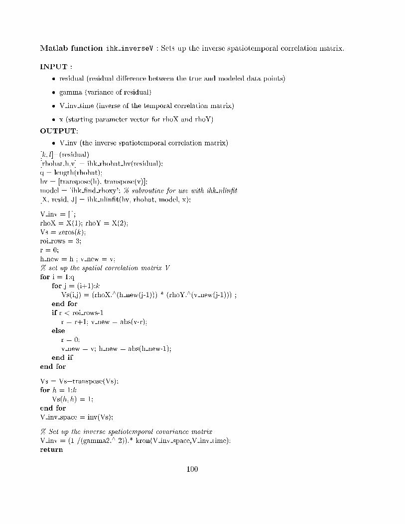
Matlab function ihk inverseV : Sets up the inverse spatiotemporal correlation matrix.
INPUT :
� residual (residual di�erence between the true and modeled data points)
� gamma (variance of residual)
� V inv time (inverse of the temporal correlation matrix)
� x (starting parameter vector for rhoX and rhoY)
OUTPUT:
� V inv (the inverse spatiotemporal correlation matrix)
[k; l]=(residual)[rhohat,h,v] = ihk rhohat hv(residual);q = length(rhohat);hv = [transpose(h), transpose(v)];model = 'ihk �nd rhoxy'; % subroutine for use with ihk nlin�t
[X, resid, J] = ihk nlin�t(hv, rhohat, model, x);
V inv = [ ];rhoX = X(1); rhoY = X(2);Vs = zeros(k);roi rows = 3;r = 0;h new = h ; v new = v;% set up the spatial correlation matrix V
for i = 1:qfor j = (i+1):k
Vs(i,j) = (rhoX.^(h new(j-1))) * (rhoY.^(v new(j-1))) ;end for
if r < roi rows-1r = r+1; v new = abs(v-r);
else
r = 0;v new = v; h new = abs(h new-1);
end if
end for
Vs = Vs+transpose(Vs);for h = 1:k
Vs(h; h) = 1;end for
V inv space = inv(Vs);
% Set up the inverse spatiotemporal covariance matrix
V inv = (1 /(gamma2.^ 2)).* kron(V inv space,V inv time);return
100
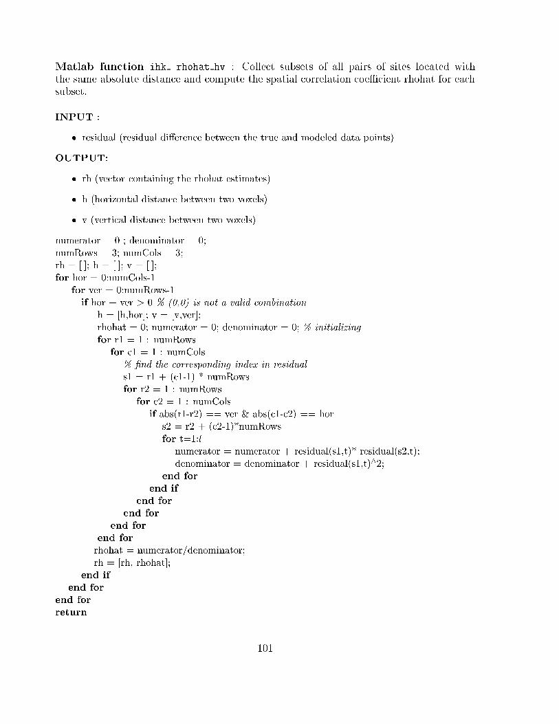
Matlab function ihk rhohat hv : Collect subsets of all pairs of sites located withthe same absolute distance and compute the spatial correlation coeÆcient rhohat for eachsubset.
INPUT :
� residual (residual di�erence between the true and modeled data points)
OUTPUT:
� rh (vector containing the rhohat estimates)
� h (horizontal distance between two voxels)
� v (vertical distance between two voxels)
numerator = 0 ; denominator = 0;numRows = 3; numCols = 3;rh = [ ]; h = [ ]; v = [ ];for hor = 0:numCols-1
for ver = 0:numRows-1if hor + ver > 0 % (0,0) is not a valid combination
h = [h,hor]; v = [v,ver];rhohat = 0; numerator = 0; denominator = 0; % initializing
for r1 = 1 : numRowsfor c1 = 1 : numCols
% �nd the corresponding index in residual
s1 = r1 + (c1-1) * numRowsfor r2 = 1 : numRows
for c2 = 1 : numColsif abs(r1-r2) == ver & abs(c1-c2) == hor
s2 = r2 + (c2-1)*numRowsfor t=1:l
numerator = numerator + residual(s1,t)* residual(s2,t);denominator = denominator + residual(s1,t)^2;
end for
end if
end for
end for
end for
end for
rhohat = numerator/denominator;rh = [rh, rhohat];
end if
end for
end for
return
101

6.5 Convolved Compartment Model
The Convolved Compartment Model presented in this work is constructed on the basis of
two articles [28, 27], in which an outline of the procedure is given. A detailed description
of the model is found in Section 5.3. There is a radical di�erence between the modeling
function, g(t; �), in this method and the Gaussian modeling function employed in the signal
description methods in Sections 5.1 and 5.2. The modeling function for the present method
is constructed from a more involved physiological point of view and attempts to modulate
transient neuronal and vascular events associated with the haemodynamic BOLD-response.
A square-wave function for the neuronal stimulation is combined (i.e. convolved) with a
vascular compartment model. An example signal with the corresponding eight parameters
is shown in Figure 6.6. Only the parameters t0 (interpreted as onset of neuronal activation)
and t1 (interpreted as duration of neuronal activation) can easily be con�rmed by visual
inspection.
Arb.
uni
ts
seconds
t� t� + t�t�
5 10 15
10
20
30 [��, ...., ��] =
[10, 0.06, 5.63, 0, 0.66, 6.11, 4.6, 1.27]
[a, t�, t� , b, γ�, γ�, γ�, γ�] =
Figure 6.6: Modeling function, g(t; �) = f(t; 0; 1; 2; 3) ? n(t; a; t0; t1) + b , for the Con-
volved Compartment Model. Note that g(t; �) = 0 in the interval 0 � t < t0
For validation, the model was tested with various sets of known parameter vectors. The
following steps were taken:
102

- Implementation of the physiological modeling function g(t; �)
- Signal construction based on the modeling function, the parameter vector used for
this construction is denoted �true and gtrue = g(t; �true)
- Selection of 8 starting parameters, � = (�0; : : : ; �7)
- Parameter estimation using the Levenberg-Marquardt procedure as implemented in
Matlab's lsqnonlin. Estimated parameter vector is denoted �est and gest = g(t; �est)
- Comparison of results. Di�erences in gest and gtrue were found from:
Æ = maxt2[a;b]
fjgtrue(t)� gest(t)jg (6.3)
in which [a; b] is the trial interval.
We de�ne
gtrue � gest if Æ � 10�3:
With this de�nition, a high temporal resolution (e.g t = 0 : 0:001 : 20) and by appropri-
ately setting the tolerance, gest were found to be equal to gtrue. However, while di�erences
between gest and gtrue were in the range of 10�3 or less, the corresponding parameter sets
were found to di�er in the order of for example 0.3-0.7 for 0 and 6.1-7.1 for 1. Hence,
two signal that are equal according to our de�nition can be constructed from a number
of relatively di�erent parameter sets. It is, however, only in the vascular parameters,
( 0; ::; 3), that the variabilities occur, the true neuronal parameters (a; t0; t1) are readily
reproduced. Our tests suggest that the landscape of the multivariate function to minimize
(Equation (5.24)) is rather shallow for the vascular parameters. This may lead to similar
sub-optimal solutions (many local minima) in a relatively wide parameter range. More-
over, Kruggel & Cramon [28] "had to resort to a costly optimization method (the genetic
algorithm)" in their optimisation step. An example of four signal shapes which are equal
according to our de�nition, with corresponding vascular parameter sets, is illustrated in
Figure 6.7.
Seeking the reasons for this behaviour in the vascular parameters, we explored the un-
derlying physiological mechanisms of the vascular component (see Figure 6.8). Vascular
geometry and distribution of oxyhaemoglobin/deoxyhaemoglobin is not easily modeled.
An essential problem is that many image voxels contain very heterogeneous distributions
103
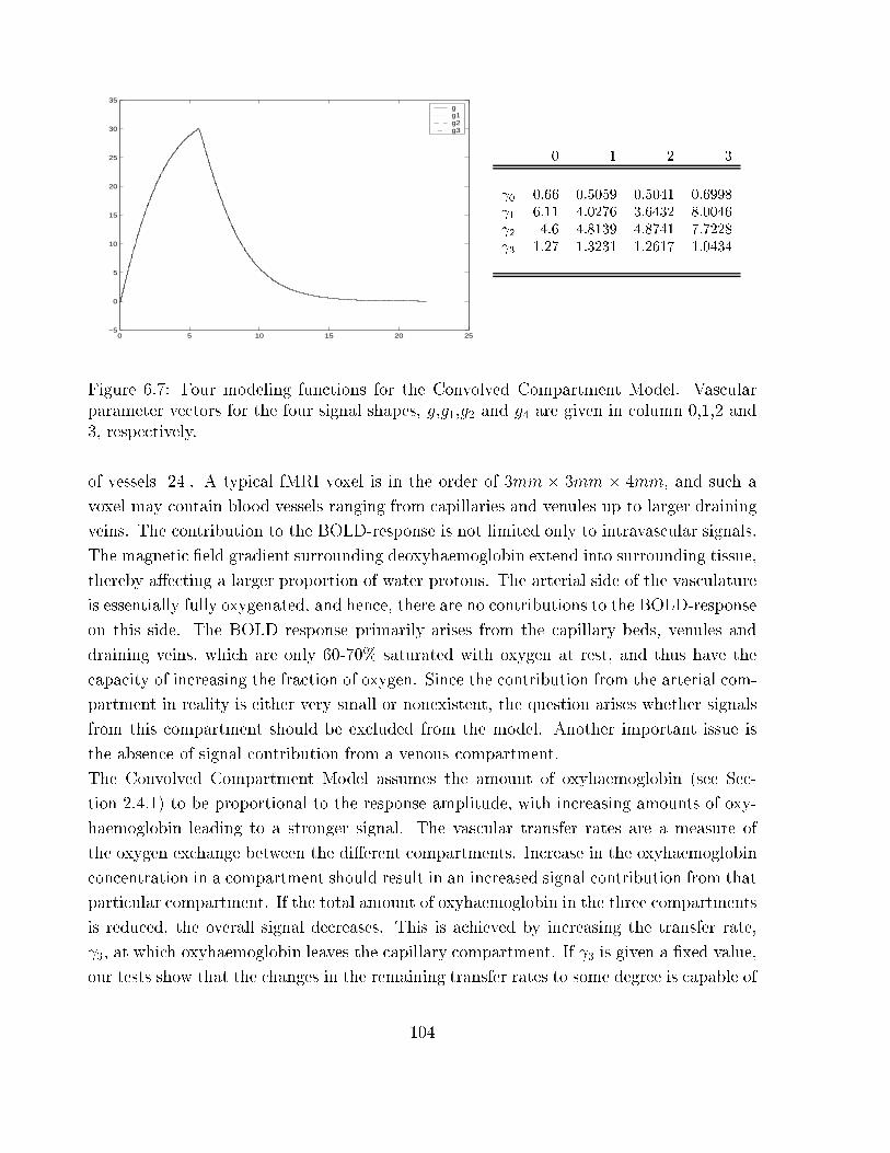
0 5 10 15 20 25−5
0
5
10
15
20
25
30
35g g1g2g3
0 1 2 3
0 0.66 0.5059 0.5041 0.6998
1 6.11 4.0276 3.6432 8.0046
2 4.6 4.8139 4.8741 7.7228
3 1.27 1.3231 1.2617 1.0434
Figure 6.7: Four modeling functions for the Convolved Compartment Model. Vascular
parameter vectors for the four signal shapes, g,g1,g2 and g4 are given in column 0,1,2 and
3, respectively.
of vessels [24]. A typical fMRI voxel is in the order of 3mm � 3mm � 4mm, and such a
voxel may contain blood vessels ranging from capillaries and venules up to larger draining
veins. The contribution to the BOLD-response is not limited only to intravascular signals.
The magnetic �eld gradient surrounding deoxyhaemoglobin extend into surrounding tissue,
thereby a�ecting a larger proportion of water protons. The arterial side of the vasculature
is essentially fully oxygenated, and hence, there are no contributions to the BOLD-response
on this side. The BOLD response primarily arises from the capillary beds, venules and
draining veins, which are only 60-70% saturated with oxygen at rest, and thus have the
capacity of increasing the fraction of oxygen. Since the contribution from the arterial com-
partment in reality is either very small or nonexistent, the question arises whether signals
from this compartment should be excluded from the model. Another important issue is
the absence of signal contribution from a venous compartment.
The Convolved Compartment Model assumes the amount of oxyhaemoglobin (see Sec-
tion 2.4.1) to be proportional to the response amplitude, with increasing amounts of oxy-
haemoglobin leading to a stronger signal. The vascular transfer rates are a measure of
the oxygen exchange between the di�erent compartments. Increase in the oxyhaemoglobin
concentration in a compartment should result in an increased signal contribution from that
particular compartment. If the total amount of oxyhaemoglobin in the three compartments
is reduced, the overall signal decreases. This is achieved by increasing the transfer rate,
3, at which oxyhaemoglobin leaves the capillary compartment. If 3 is given a �xed value,
our tests show that the changes in the remaining transfer rates to some degree is capable of
104

(f1) Arterial Compartment
(f2) Capillary Compartment
(f3) Tissue Compartment
Venous Compartment
�� ��
��
��
Figure 6.8: Movement of oxygen in vascular and tissue compartments. Modi�ed from Kruggel
& Cramon[1999]
cancelling out one another. More speci�cally, an increase in 0 and 2 leads to a higher con-
centration of oxyhaemoglobin in the capillary compartment (see Figure 6.8). These e�ects
may, however, be counteracted by an increase in 1. Only two transfer rates, 1 and 2,
directly a�ects the oxyhaemoglobin concentration of the tissue compartment. Decreasing
1 reduces the signal, but this e�ect may conveniently be cancelled out by a simultaneous
decrease in 2. From a physiological point of view it is therefore reasonable that several
combinations of the vascular parameters may lead to similar signal amplitudes. Another
important issue regarding present fMRI techniques is the limited number of time steps
that can be measured per trial. This puts restrictions on the maximum number of model
parameters that can be reasonably estimated for any model function.
Tests were also performed separately on the vascular model, thereby eliminating possible
in uence by the neuronal parameters. The vascular component of the Convolved Com-
partment Model, f = f1 + f2 + f3, is given by Equation (5.21) (illustrated in Figure 6.8).
Estimation results from these tests did not contribute any signi�cant improvement.
Signal contribution from the di�erent compartments of the Convolved Compartment Model
can also be regarded separately. Since the BOLD-response primarily arises from capillary,
tissue and venules, the focus should be on the capillary compartment alone or on the
capillary and the tissue compartments. This modeling context still su�er from the absence
of venous contributions. To explore this approach, the convolution in Equation (5.18) was
modi�ed to only consider the capillary signal contribution, that is
y(s; t) = f2(t) ? n(t) + b + �(s; t):
An example signal with the corresponding parameters is shown in Figure 6.9. Valida-
tion was performed as previously described. By appropriately setting the tolerance, and
105

applying a high temporal resolution, we found
gest � gtrue and �true � �est
However, the number of observations per trial in fMRI data is low compared to the temporal
resolution employed for the present evaluations. Reducing the number of time points to
12-22 observations per trial lead to relatively large departures from the true (vascular)
parameter values.
Arb.
uni
ts
seconds
t� t� + t�t�
5 10 15
2
4
6 [��, ��, �� , ��, ��, ��, ��, ��] =
[10, 0.06, 5.63, 0, 0.66, 6.11, 4.6, 1.27]
Figure 6.9: Modeling function for the capillary compartment of the Convolved Compart-
ment Model
In the modeling of the BOLD-response it is important that the selected modeling functions
span the space of potential responses. The shape of this modeling function di�ers from
the shape of the Gaussian function, and may therefore be more suitable for modeling some
types of BOLD-responses. The question arises, however, as to what extent conclusions
regarding physiological characteristics, especially the vascular components, can be drawn.
Temporal and spatial correlations in the noise are estimated in the same way as for
the Kruggel & Cramon Model. The noise correlation matrix, V�1, is then subject to a
Choleskys factorization as described in the previous section. One parameter set is obtained
for each trial in each ROI time series. Expensive estimation algorithms, such as genetic al-
gorithms and simulated annealing, has been suggested for the minimization problem [28].
106
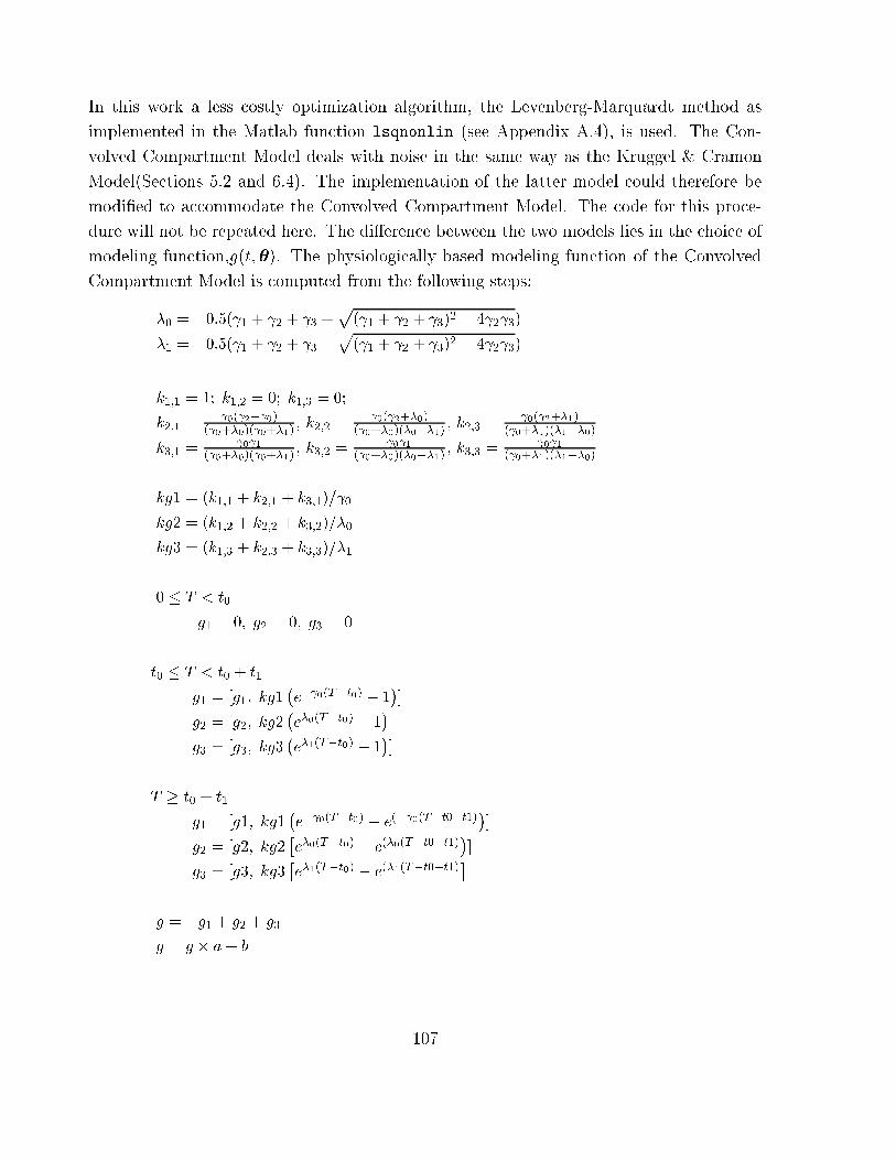
In this work a less costly optimization algorithm, the Levenberg-Marquardt method as
implemented in the Matlab function lsqnonlin (see Appendix A.4), is used. The Con-
volved Compartment Model deals with noise in the same way as the Kruggel & Cramon
Model(Sections 5.2 and 6.4). The implementation of the latter model could therefore be
modi�ed to accommodate the Convolved Compartment Model. The code for this proce-
dure will not be repeated here. The di�erence between the two models lies in the choice of
modeling function,g(t; �). The physiologically based modeling function of the Convolved
Compartment Model is computed from the following steps:
�0 = �0:5( 1 + 2 + 3 +p( 1 + 2 + 3)2 � 4 2 3)
�1 = �0:5( 1 + 2 + 3 �p( 1 + 2 + 3)2 � 4 2 3)
k1;1 = 1; k1;2 = 0; k1;3 = 0;
k2;1 = 0( 2� 0)
( 0+�0)( 0+�1), k2;2 =
0( 2+�0)( 0+�0)(�0��1)
, k2;3 = 0( 2+�1)
( 0+�1)(�1��0)
k3;1 = 0 1
( 0+�0)( 0+�1), k3;2 =
0 1( 0+�0)(�0��1)
, k3;3 = 0 1
( 0+�1)(�1��0)
kg1 = (k1;1 + k2;1 + k3;1)= 0
kg2 = (k1;2 + k2;2 + k3;2)=�0
kg3 = (k1;3 + k2;3 + k3;3)=�1
0 � T < t0
g1 = 0; g2 = 0; g3 = 0
t0 � T < t0 + t1
g1 = [g1; kg1�e� 0(T�t0) � 1
�]
g2 = [g2; kg2�e�0(T�t0) � 1
�]
g3 = [g3; kg3�e�1(T�t0) � 1
�]
T � t0 + t1
g1 = [g1; kg1�e� 0(T�t0) � e
(� 0(T�t0�t1)�]
g2 = [g2; kg2�e�0(T�t0) � e
(�0(T�t0�t1)�]
g3 = [g3; kg3�e�1(T�t0) � e
(�1(T�t0�t1)�
g = �g1 + g2 + g3
g = g � a+ b
107

Chapter 7
Experimental Results
This chapter reports of experiments on synthetic as well as real data. The signal detection
problem is assessed by ANOVA (Section 4.1) on a real er-fMRI data set. The main part of
this chapter is, however, dedicated to the signal description problem which can for example
be formulated in terms of introduction and estimation of physiologically interpretable pa-
rameters like lag (time to maximum response intensity), dispersion (duration of response)
and gain response intensity/strength) or vascular transfer rates between di�erent physi-
ological tissue compartments. The methods selected for this purpose are the Nonlinear
Least Squares Model (Section 5.1), the Kruggel & Cramon Model (Section 5.2) and the
Convolved Compartment Model (Section 5.3). The ability to model the BOLD-response
in er-fMRI data, with increasing noise levels, have been explored. Another issue of inter-
est is whether the parameters are capable of re ecting physiological characteristics of the
BOLD-response itself and/or the underlying neuronal activity.
Section 7.1 deals with experiments on synthetic data. These experiments are concerned
exclusively with the signal description problem. In Section 7.2 real data experiments
dealing with both the signal detection problem and the signal description problem will be
presented. Experiments on real data with the Convolved Compartment Model have not
carried out.
7.1 Synthetic Data
7.1.1 Construction of Synthetic Data
Simulated event-related data-sets have been used for the evaluation of the signal description
models in this thesis. A dataset from a recent single trial er-fMRI experiment on language
processing was selected for this purpose. This dataset was acquired on a Siemens Vision
108
Plus 1.5 Tesla Scanner at Haukeland University Hospital. We used gradient echo, with an
echo time TE = 60 msec, TR = 0.6 sec and ip angle = 90Æ (FOV = 200mm), and a total
of 501 echo planar images (EPI see Section 2.2.7) were acquired. Each image consisted
of 20 slices of 64 �64 voxel resolution and spatial resolution 3.13�3.13�4 mm, no gap
between consecutive slices. A corresponding anatomical image was acquired in the same
session.
The data set was preprocessed and analyzed with SPM99 (see Appendix A.3) after which
25 non-activated brain patches were located. Synthetic ROI time series were constructed
by modulating various prototypical BOLD-responses with known properties (spatial distri-
bution, temporal shape; Figures 7.4 and 7.5) onto these patches. Five di�erent prototypical
BOLD-responses with sampling frequency of 12 time points per single trial and 2 seconds
between each time point, were explored. With this trial period of 12 time points, a total
of 40 prototypical BOLD-responses were modulated onto each voxel time series.
In real fMRI data sets, the BOLD-response have been reported to be in the order of about
1-10% relative to mean signal intensity level. Boynton et al. [5] found that activation
modulates 5-10% above and below baseline whereas Parrish et al. [36] estimates brain
activations to be 1-5% relative to mean signal intensity level (at 1.5 Tesla). The synthetic
data should be tested with similar Signal to Noise Ratio (SNR, see Section 2.2.8).
We found a high spatial correlation in the fMRI voxel time courses used for the synthetic
data set. For the spatial pattern illustrated in Figure 7.4, correlation coeÆcients in the x
and y-directions (see Section 5.2) were calculated to be in the range 0.95-1.0 for prepro-
cessed and smoothed data, and 0.6-1.0 prior to preprocessing. Since Kruggel & Cramon [27]
reported of spatial correlation coeÆcients in the range of 0.4-0.6 for smoothed data, and
0.1-0.3 for non-�ltered data, two additional data sets from two di�erent experiments, ac-
quired at Haukeland University Hospital, were also investigated. Correlation coeÆcients
for both data sets con�rmed a high spatial correlation. Figures 7.1, 7.2 and 7.3 illustrates
the spatial correlations in the three data sets.
The noisy component of fMRI data is assumed to have a normal distribution (see Sec-
tion 3.2). Normality tests according to Lilliefors and Bera-Jarque con�rmed this assump-
tion for all three data sets.
109

0 5 10 15 20 25 30 35 40 45500
510
520
530
540
550
560
570
580
Figure 7.1: Signal intensity versus time (i.e voxel time courses) in smoothed fMRI data
for 9 neighbouring voxels in a word recognition single trial er-fMRI experiment. x-axis
represents time (seconds) and y-axis the signal intensity (arbitrary units). Note the spatial
correlation of the time series.
0 5 10 15 20 25 30 35580
600
620
640
660
680
700
720
seconds
arb. u
nits
Figure 7.2: Signal intensity versus time (i.e voxel time courses) in smoothed fMRI data
for 9 neighbouring voxels in a �nger tapping er-fMRI experiment. x-axis represents time
(seconds) and y-axis the signal intensity (arbitrary units). Note the spatial correlation of
the time series.
110

0 5 10 15 20 25 30 35495
500
505
510
515
520
525
530
535
seconds
arb. u
nits
Figure 7.3: Signal intensity versus time (i.e voxel time courses) in smoothed fMRI data for
9 neighbouring voxels in a dichotic listening, er-fMRI experiment. x-axis represents time
(seconds) and y-axis the signal intensity (arbitrary units). Note the spatial correlation of
the time series.
7.1.2 Experimental Design
The BOLD-response is reported to vary in duration, time to maximum as well as rise and
fall times. For the experiments in this thesis �ve di�erent prototypical BOLD-responses,
with varying spatial and temporal characteristics, were constructed. Figure 7.4 depict three
of these shapes and their spatial pattern. These three shapes were constructed from the
Gaussian function (see Equation (3.6)), and were employed in the experiments involving
the Nonlinear Least Squares Model in Section 7.1.3 and the Kruggel & Cramon Model in
Section 7.1.4. True parameters for dispersion and lag are given in Table 7.1.2. Baseline
correction in uence the values of gain and baseline. True values for these parameters must
therefore be established separately for each voxel time course. The three di�erent Gaussian
shapes were modulated onto each of the 25 non-activated brain patches yielding a total of
75 ROI time series.
For the experiments in Section 7.1.5 with the Convolved Compartment Model, two di�erent
prototypical BOLD-responses (see Figure 7.5) were constructed from Equation (5.18) with
spatial pattern as illustrated in Figure 7.4a. From these two shapes a total of 50 synthetic
ROI time series were constructed.
The prototypical BOLD-responses were modulated onto the 25 brain patches with signal
111
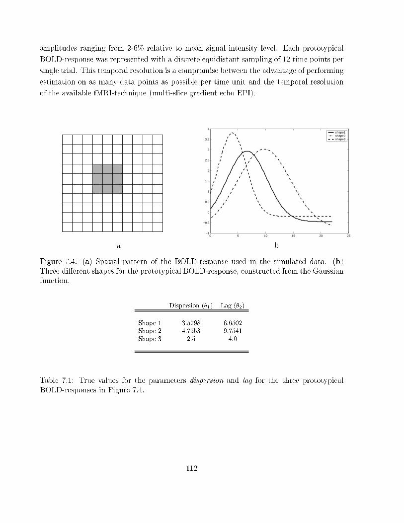
amplitudes ranging from 2-6% relative to mean signal intensity level. Each prototypical
BOLD-response was represented with a discrete equidistant sampling of 12 time points per
single trial. This temporal resolution is a compromise between the advantage of performing
estimation on as many data points as possible per time unit and the temporal resolution
of the available fMRI-technique (multi-slice gradient echo EPI).
0 5 10 15 20 25−1
−0.5
0
0.5
1
1.5
2
2.5
3
3.5
4shape1shape2shape3
a b
Figure 7.4: (a) Spatial pattern of the BOLD-response used in the simulated data. (b)
Three di�erent shapes for the prototypical BOLD-response, constructed from the Gaussian
function.
Dispersion (�1) Lag (�2)
Shape 1 3.5798 6.6502
Shape 2 4.7553 9.7541
Shape 3 2.5 4.0
Table 7.1: True values for the parameters dispersion and lag for the three prototypical
BOLD-responses in Figure 7.4.
112

0 5 10 15 20 250
5
10
15
20
25
30
35
Seconds
Arb.
Uni
ts
shape 4shape 5
4 5
�0 7 4
�1 0.05 0.25
�2 4.6 8
�3 0 0
�4 0.4 0.7
�5 8.51 6.11
�6 8.6 6.6
�7 3.17 2.5
Figure 7.5: Two di�erent synthetic BOLD-responses constructed from the modeling func-
tion in the Convolved Compartment Model. True values for the parameter vector, �, are
given in 4 and 5.
The prototypical BOLD-responses were adjusted to both signal amplitude and mean sig-
nal intensity level. Matlab code for this procedure is shown below (ihk synt data). A
subroutine (ihk update y) takes care of the estimation of the true parameters after the
prototypical BOLD-response has been adjusted to mean signal intensity level and desired
signal amplitude. Estimation procedure for �nding the true parameters depends on whether
the prototypical BOLD-response was constructed from the Gaussian function or from the
modeling function of the Convolved Compartment Model. The subroutine takes as input
the estimation procedure and the prototypical BOLD-response, and returns a new pro-
totypical BOLD-response which can be modulated onto the non-activated brain patch.
Figure 7.6 shows a synthesized signal collected from 4 neighboring voxels.
Matlab function ihk synt data :
INPUT:
� y (vector with prototypical BOLD-response)
� ROI (non-activated brain patch, 3� 3 voxel grid)
� signampl (desired signal amplitude)
� est model (optimization method for �nding the true parameters. Options are "gauss" or"convcomp")
113

OUTPUT:
� ROI new (the new ROI with synthetic activation/BOLD-response)
� theta true (true parameters for the prototypical BOLD-response)
[k;N ] = size(ROI); % k voxels and N time points
l = length(y); % l time points per trial
residual = ROI;
% �nd mean voxel value as the mean over all time steps for each voxel in a ROI
mean voxel value = mean(transpose(ROI));
% compute scaling factor for the prototypical BOLD-response relative to mean signal intensity
level
rise voxels = mean voxel value.* signampl;scale voxels = rise voxels ./ max(y);
% adjust y
scale average = mean(scale voxels);y new = scale average .* y;
% update y new and �nd true parameters
t=[0 : 2 : l]; % 2 seconds between each time point
[theta true, y update] = ihk update y(y new,' est model',t);
% modulate the signal on top of the noise
for voxel = 1 : kfor trial = 1 : l : N
if (trial+(l� 1)) � NROI(voxel,trial:(trial+(l�1))) = ( ROI(voxel,trial:(trial+(l�1)))+ transpose(y update));
end if
end for
end for
% correct for baseline
meanresidual = mean(transpose(residual));for i = 1:k
ROI(i,:) = ( ROI(i,:) - meanresidual(i) );end for
return;
Matlab function ihk update y :
INPUT:
� y (vector with prototypical BOLD-response)
� est model (optimization method)
114
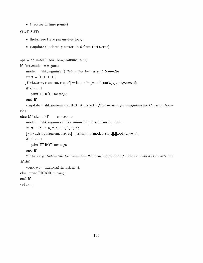
� t (vector of time points)
OUTPUT:
� theta true (true parameters for y)
� y update (updated y constructed from theta true)
opt = optimset('TolX',1e-5,'TolFun',1e-8);
if 'est model' == gauss
model = 'ihk argmin'; % Subroutine for use with lsqnonlin
start = [1, 1, 1, 1];
[ theta true, resnorm, res, ef] = lsqnonlin(model,start,[],[],opt,y new,t);
if ef �= 1
print ERROR message
end if
y update = ihk gaussmodelHR(theta true,t); % Subroutine for computing the Gaussian func-
tion
else if 'est model' == convcomp
model = 'ihk argmin cc; % Subroutine for use with lsqnonlin
start = [5, 0.06, 6, 0.1, 1, 7, 7, 2];
[ theta true, resnorm, res, ef] = lsqnonlin(model,start,[],[],opt,y new,t);
if ef �= 1
print ERROR message
end if
% ihk cc g: Subroutine for computing the modeling function for the Convolved Compartment
Model
y update = ihk cc g(theta true,t);
else print ERROR message
end if
return;
115
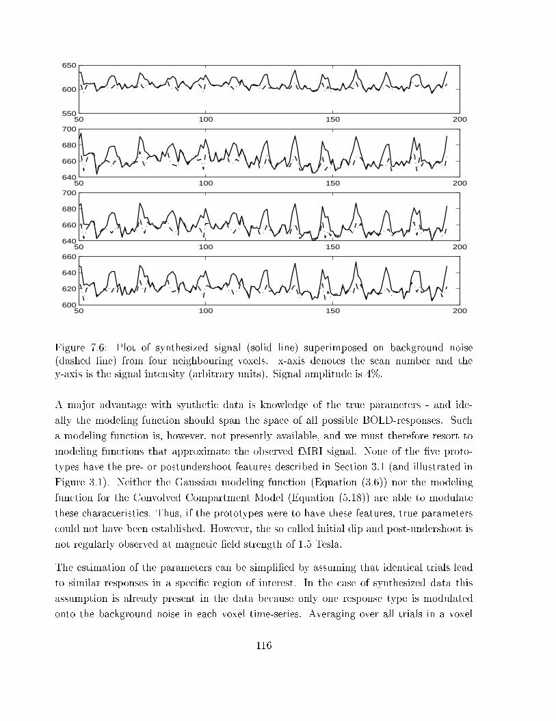
50 100 150 200550
600
650
50 100 150 200640
660
680
700
50 100 150 200640
660
680
700
50 100 150 200600
620
640
660
Figure 7.6: Plot of synthesized signal (solid line) superimposed on background noise
(dashed line) from four neighbouring voxels. x-axis denotes the scan number and the
y-axis is the signal intensity (arbitrary units). Signal amplitude is 4%.
A major advantage with synthetic data is knowledge of the true parameters - and ide-
ally the modeling function should span the space of all possible BOLD-responses. Such
a modeling function is, however, not presently available, and we must therefore resort to
modeling functions that approximate the observed fMRI signal. None of the �ve proto-
types have the pre- or postundershoot features described in Section 3.1 (and illustrated in
Figure 3.1). Neither the Gaussian modeling function (Equation (3.6)) nor the modeling
function for the Convolved Compartment Model (Equation (5.18)) are able to modulate
these characteristics. Thus, if the prototypes were to have these features, true parameters
could not have been established. However, the so called initial dip and post-undershoot is
not regularly observed at magnetic �eld strength of 1.5 Tesla.
The estimation of the parameters can be simpli�ed by assuming that identical trials lead
to similar responses in a speci�c region of interest. In the case of synthesized data this
assumption is already present in the data because only one response type is modulated
onto the background noise in each voxel time-series. Averaging over all trials in a voxel
116

will reduce the noise and approximate the true signal (See Section 4.1). The Nonlinear
Least Squares Model in experiment I explores these issues. Experiment II and III covers
the Kruggel & Cramon Model and the Convolved Compartment Model, respectively.
117

7.1.3 Experiment I: Nonlinear Least Squares Model
In the Nonlinear Least Squares Model noise is reduced by averaging over multiple trials
(see Figure 7.7). Given the 75 synthetic ROI's (25 ROI time series for each of the three
prototypical BOLD-responses (see Section 7.1.2)), time-locked to stimulus averaging over
all 40 trials in each voxel in all ROI time series was performed. Parameter estimates were
obtained using the Gauss-Newton Method as implemented in nlinfit. Signal amplitudes
ranged from 2-6% relative to mean signal intensity level. For all voxel time series a set of
parameter estimates, accompanied by 95% con�dence intervals (according to the method in
Matlab's nlparci) was obtained for each of the �ve amplitude settings. Visual inspection of
synthesized and modeled signals were carried out for all shapes in all voxels and for all signal
amplitudes. A good �t was generally found for signal amplitudes ranging from 4-5%. For
signal amplitudes of 2-3% the synthesized signal was in some voxels distorted by noise, and
thereby not easily modeled with the Gaussian modeling function. All the true parameter
values, (�0; �1; �2; �3), were, however, found to be within the 95% con�dence intervals of the
estimated values (cfr Table 7.1.3). Figures 7.8, 7.9, 7.10 and 7.11 illustrates the averaged
prototypical BOLD-responses together with the modeled signal for a representative ROI
time series. Signal amplitudes were 4% for the �rst three examples and 2% for the last
example. Summary of results for prototypical BOLD-response, shape 3 in six representative
ROI's are presented in Table 7.1.3. The table shows the average (parameter vector and
95% con�dence intervals) over the nine estimates obtained for each ROI time series.
T (trial interval )
Averaged trial time course
T
Figure 7.7: Averaged responses in er-fMRI. Averaging is performed over all trials of the
same type. The magnitude of the noisy component is reduced, but not that of the repeated
signal (Modi�ed from R. Buckner, HBM 2000).
118

0 10 20 30−5
0
5
10Voxel : 1
0 10 20 30−5
0
5
10Voxel : 2
0 10 20 30−5
0
5
10Voxel : 3
0 10 20 30−10
−5
0
5
10Voxel : 4
0 10 20 30−5
0
5
10Voxel : 5
0 10 20 30−5
0
5
10Voxel : 6
0 10 20 30−10
−5
0
5
10Voxel : 7
0 10 20 30−5
0
5
10Voxel : 8
0 10 20 30−5
0
5
10Voxel : 9
averaged signalmodel
Figure 7.8: Synthetic data, Experiment I, results from estimation of parameters for the
synthetic shape 1 (cfr. Figure 7.4). Time-locked to stimulus averaging of synthetic time
course over all trials is denoted by star dots. The estimated model signal time course is
denoted by solid line. Signal amplitude is 4%.
0 10 20 30−10
0
10
20
30Voxel : 1
0 10 20 30−10
0
10
20
30Voxel : 2
0 10 20 30−10
0
10
20
30Voxel : 3
0 10 20 30−10
0
10
20
30Voxel : 4
0 10 20 30−10
0
10
20
30Voxel : 5
0 10 20 30−10
0
10
20
30Voxel : 6
0 10 20 30−10
0
10
20
30Voxel : 7
0 10 20 30−10
0
10
20
30Voxel : 8
0 10 20 30−10
0
10
20
30Voxel : 9
averaged signalmodel
Figure 7.9: Synthetic data, Experiment I, results from estimation of parameters for the
prototypical BOLD-response, shape 2 (cfr. Figure 7.4). Time-locked to stimulus averaging
of synthetic time course over all trials is denoted by star dots. The estimated model signal
time course is denoted by solid line. Signal amplitude is 4%.
119

0 10 20 30−5
0
5
10
15Voxel : 1
0 10 20 30−5
0
5
10
15Voxel : 2
0 10 20 30−5
0
5
10
15Voxel : 3
0 10 20 30−5
0
5
10
15Voxel : 4
0 10 20 30−5
0
5
10
15Voxel : 5
0 10 20 30−5
0
5
10
15Voxel : 6
0 10 20 30−5
0
5
10
15Voxel : 7
0 10 20 30−5
0
5
10
15Voxel : 8
0 10 20 30−5
0
5
10
15Voxel : 9
averaged signalmodel
Figure 7.10: Synthetic data, Experiment I, results from estimation of parameters for the
prototypical BOLD-response, shape 3 (cfr. Figure 7.4). Time-locked to stimulus averaging
of synthetic time course over all trials is denoted by star dots. The estimated model signal
time course is denoted by solid line. Signal amplitude is 4%.
0 10 20 30−5
0
5
10
15Voxel : 1
0 10 20 30−5
0
5
10
15Voxel : 2
0 10 20 30−5
0
5
10
15Voxel : 3
0 10 20 30−5
0
5
10
15Voxel : 4
0 10 20 30−5
0
5
10
15Voxel : 5
0 10 20 30−5
0
5
10
15Voxel : 6
0 10 20 30−5
0
5
10
15Voxel : 7
0 10 20 30−5
0
5
10
15Voxel : 8
0 10 20 30−5
0
5
10
15Voxel : 9
averaged signalmodel
Figure 7.11: Synthetic data, Experiment I, results from estimation of parameters for the
prototypical BOLD-response, shape 2 (cfr. Figure 7.4). Time-locked to stimulus averaging
of synthetic time course over all trials is denoted by star dots. The estimated model signal
time course is denoted by solid line. Signal amplitude is 2%.
120

Location �0 (gain) �1 (dispersion) �2 (lag) �3 (baseline)
ROI 1 True 56.4506 2.5000 4.0000 -1.1290
Estimated 59.4764 �5.46551 2.5911 � 0.2279 3.8428 � 0.1956 -1.3617 � 0.7320
ROI 2 True 53.7129 2.5000 4.0000 -1.0743
Estimated 56.2737 �4.7608 2.5643 �0.2077 3.8630 � 0.1790 -1.2725 � 0.64350
ROI 3 True 58.9247 2.5000 4.0000 -1.1785
Estimated 61.3766 �5.5697 2.5914 �0.2249 3.8909 � 0.1934 -1.3221 � 0.7488
ROI 4 True 70.2582 2.5000 4.0000 -1.4052
Estimated 74.0736 � 9.2802 2.6510 �0.3144 4.0306 � 0.2693 -1.6675 � 1.2337
ROI 5 True 59.4794 2.5000 4.0000 -1.1896
Estimated 63.2248 �5.7620 2.5828 � 0.2237 3.9949 � 0.1928 -1.4817 � 0.7781
ROI 6 True 62.6489 2.5000 4.0000 -1.2530
Estimated 66.9899 � 6.5016 2.6661 � 0.2432 3.9187 � 0.2082 -1.2530 � 0.8639
Table 7.2: Synthetic data, Experiment I, averaged parameter estimates for the synthesized
signal(prototypical BOLD-response, shape 3) in selected regions. Parameters and 95%
con�dence intervals averaged over each ROI.
Gain was found to increase linearly with signal amplitude. There was a tendency towards
overestimated gain values for prototypical BOLD-response, shapes 1 and 3, whereas gain
for shape 2 generally was estimated to be below the true value. Dispersion values were
overestimated for shape 1 and 3, while a slight underestimation was seen for shape 2
(see Figure 7.12 a,b and c). These asymmetries increased for cases of low signal to noise
ratio (SNR, see Section 2.2.8). Lag was slightly underestimated for all three shapes (see
Figure 7.12 d,e and f).
The parameter estimates were plotted with signal amplitudes ranging from 2% to 5%
relative to mean signal intensity level. For increasing SNR, the estimated parameters
converge toward the true value. Figure 7.13 shows the resulting dispersion and lag values
for a representative ROI time series.
Based on the test results the estimation procedure is assumed to be stable against noise
levels typically found in er-fMRI data.
Normality (tested according to Lilliefors and Bera-Jarque (see Appendix A.4)) in the resid-
ual distributions after estimation were ful�lled for all regions. Q-Q plots also revealed a
high conformance with a normal distribution.
121

Regarding physiological interpretations of the estimated parameters gain, dispersion and
lag (which might express neuronal processing strength, processing duration or asynchrony
and processing delay, respectively) we plotted the three parameter estimates in a 3D fea-
ture plot. This plot will thus indicate if the joint distribution of these parameters are
suÆciently separated to discriminate between di�erent types of BOLD-responses which
might give information about underlying neuronal processing mechanisms. Feature plots
were generated for all ROI time series and all signal amplitudes. Even for small signal am-
plitudes, the three di�erent shapes explored in this experiment can easily be distinguished
and if desired mapped to the corresponding anatomical images. Example feature plots for
the three di�erent shapes are given in Figures 7.14 and 7.15. Signal amplitudes are 2 and
5%. In both examples the three prototypical BOLD-responses are easily distinguished.
The performed experiments demonstrates that the averaging approach for the present
model leads to robust parameter estimates for the three prototypical BOLD-responses.
The model is stable against noise levels commonly found in fMRI data. Furthermore, the
procedure is easy to implement and computation cost is low.
0 2 4 6 83
3.5
4
4.5DISPERSION, SHAPE 1
seco
nds
0 2 4 6 86
6.5
7LAG, SHAPE 1
seco
nds
0 2 4 6 83
4
5
6DISPERSION, SHAPE 2
seco
nds
0 2 4 6 89.4
9.6
9.8
10LAG, SHAPE 2
seco
nds
1 2 3 4 5 6 7
2.4
2.6
2.8
3
3.2DISPERSION, SHAPE 3
% signal amplitude
seco
nds
0 2 4 6 83
3.5
4
4.5LAG, SHAPE 3
% signal amplitude
seco
nds
Figure 7.12: Synthetic data, Experiment I, Dependency of the parameters on the signal
amplitude, here represented by dispersion (a,b,c) and lag (d,e,f) values. Signal amplitudes
ranges from 2 to 6% relative to the mean intensity level.
122

2 2.5 3 3.5 4 4.5 53.4
3.5
3.6
3.7
3.8Dispersion
true value 3.579800e+000
2 2.5 3 3.5 4 4.5 54.4
4.5
4.6
4.7
4.8true value 4.755300e+000
2 2.5 3 3.5 4 4.5 52.4
2.5
2.6
2.7
2.8true value 2.500000e+000
2 2.5 3 3.5 4 4.5 56.4
6.5
6.6
6.7
6.8Lag
true value 6.650200e+000
2 2.5 3 3.5 4 4.5 59.6
9.7
9.8
9.9
10true value 9.754100e+000
2 2.5 3 3.5 4 4.5 53.7
3.8
3.9
4
4.1true value 4
Dispersion Lag
Figure 7.13: Synthetic data, Experiment I, robustness to noise in the parameters dispersion
and lag. Signal amplitudes ranging from 2% to 5% relative to mean signal intensity.
3035
4045
5055
3
3.5
4
4.5
2
4
6
8
10
12
gaindispersion
lag
shape1shape2shape3
Figure 7.14: Synthetic data, Experiment I, example feature plot. Each prototypical BOLD-
response is mapped in 3D feature space with a �lled symbol. "Empty" symbols shows the
projections from 3D feature space to each of the three planes. Signal amplitude is only 2%
123

80
100
120
140
3
3.5
4
4.5
2
4
6
8
10
12
gaindispersion
lag
shape1shape2shape3
Figure 7.15: Synthetic data, Experiment I, example feature plot. Each prototypical BOLD-
response is mapped in 3D feature space with a �lled symbol. "Empty" symbols shows the
projections from 3D feature space to each of the three planes. Signal amplitude is 5%
124

7.1.4 Experiment II: Kruggel & Cramon Model
This section reports on several experiments performed with the Kruggel & Cramon Model.
From the synthetic dataset described in Section 7.1, a total of 20 ROI time series, each
modulated with three di�erent prototypical shapes (see Section 7.1.2), were selected. From
each ROI time series 20 trials were extracted, each of which was sampled with 12 time
points. Thus, a total of 1200 parameter estimates were obtained for each of the 5 signal
amplitudes.
Kruggel & Cramon [27] suggests the Nelder & Mead Downhill simplex method for the
parameter estimation. For the experiments in this section, this method together with the
Levenberg-Marquardt method, was considered. Figure 7.16 shows the results from the
estimation of eight consecutive trials. This signal is constructed from the prototypical
BOLD-response, shape 1, and signal amplitude is 4%.
Tests of normality in the residuals were ful�lled for the majority of trials. These �ndings
agreed with visual inspection of QQ-plots. Deviations were mainly present in trials with
a low Signal to Noise Ratio and. In Table 7.3 summary statistics for prototypical BOLD-
response, shape 3, in six sample ROI time series is given. The table displays parameter sets
averaged over 20 ROI's in each of the six ROI time series. The estimation algorithm for
this example is the Levenberg-Marquardt method and the signal amplitude is 4%. Each
parameter estimate is presented with a 95% con�dence interval (Matlab's nlparci was
used for this purpose). The ROI time series listed in this table are identical with the ROI
time series in Table 7.1.3.
To assess the robustness of the signal to increasing noise levels, all ROI's were evaluated for
signal amplitudes ranging from 2-6% relative to the mean signal intensity level. An aver-
aged parameter estimate was computed for each ROI time series resulting in 60 parameter
sets for each signal amplitude. Results from estimation with the Levenberg-Marquardt
method are shown in Figure 7.17. Figure 7.18 shows the results from estimation with
Nelder & Mead Downhill simplex method. The largest departures from the true parameter
values were found with the Nelder & Mead Downhill simplex method. This procedure
also produced poor parameter estimates more frequently than the Levenberg-Marquardt
method. This is especially noticeable for dispersion values of the prototypical BOLD-
response, shape 2, and lag values of shape 3. Moreover, computation times per parameter
estimate for the Levenberg-Marquardt method are approximately twice as fast compared
to the Nelder & Mead Downhill simplex method. Based on these results we favor the
Levenberg-Marquardt method for the parameter estimation of the present model.
125

0 10 20 30 40 50 60 70 80 90 100−20
−10
0
10
20
30
40
Time points
Arbit
rary u
nits
Model with estimated parametersSynt. signal in ROI
Figure 7.16: Synthetic data, Experiment II, prototypical BOLD-response, shape 1, eight
consecutive trials with 12 time points each. Signal amplitude in this example is 4%
Location �0 (gain) �1 (dispersion) �2 (lag) �3 (baseline)
ROI 1 True 56.4506 2.5000 4.0000 -1.1290
Estimated 65.0547 �24.7370 2.6981 � 0.9803 3.9296 � 0.8185 -1.326 �3.1653
ROI 2 True 53.7129 2.5000 4.0000 -1.0743
Estimated 60.6850 � 23.3116 2.5060 � 0.9965 3.9230 � 0.8223 -1.3395 � 3.0044
ROI 3 True 58.9247 2.5000 4.0000 -1.1785
Estimated 60.1267 �15.7736 2.5063 � 0.5937 3.9961 � 0.5214 -0.4993 � 2.3512
ROI 4 True 70.2582 2.5000 4.0000 -1.4052
Estimated 74.6687 � 32.6574 2.6125 � 1.1589 4.1944 � 0.9362 -0.7206 � 4.1922
ROI 5 True 59.4794 2.5000 4.0000 -1.1896
Estimated 60.2500 � 21.3372 2.3279 � 0.9090 4.2150 � 0.7358 -1.1556 � 2.9579
ROI 6 True 62.6489 2.5000 4.0000 -1.2530
Estimated 69.4466 � 17.2870 2.7227 � 0.7142 4.0630 � 0.5755 -1.7150 � 2.1327
Table 7.3: Synthetic data, Experiment II, parameter estimates for the prototypical BOLD-
response, shape 3, in selected regions. Parameters and con�dence intervals (95%) averaged
over 20 ROI's in each ROI time series.
126

0 2 4 6 82.5
3
3.5
4DISPERSION, SHAPE 1
seco
nd
s
0 2 4 6 86
6.5
7
7.5LAG, SHAPE 1
seco
nd
s0 2 4 6 8
3
4
5
6DISPERSION, SHAPE 2
seco
nd
s
0 2 4 6 88.5
9
9.5
10LAG, SHAPE 2
seco
nd
s
1 2 3 4 5 6 7
2.4
2.6
2.8
3
3.2DISPERSION, SHAPE 3
% signal amplitude
seco
nds
0 2 4 6 83
4
5
6LAG, SHAPE 3
% signal amplitude
seco
nds
Figure 7.17: Synthetic data, Experiment II, dependency of the parameters, represented by
dispersion and lag, on the signal amplitude. Signal amplitudes are 2-6% relative to mean
signal intensity level. Estimation procedure : Nonlinear Least Squares by the Levenberg-
Marquardt method
127

0 2 4 6 82
2.5
3
3.5
4DISPERSION, SHAPE 1
seco
nd
s
0 2 4 6 86
6.5
7
7.5LAG, SHAPE 1
seco
nd
s0 2 4 6 8
0
5
10
15
20DISPERSION, SHAPE 2
seco
nd
s
0 2 4 6 88.5
9
9.5
10LAG, SHAPE 2
seco
nd
s
1 2 3 4 5 6 7
2.4
2.6
2.8
3
3.2DISPERSION, SHAPE 3
% signal amplitude
seco
nds
0 2 4 6 8−30
−20
−10
0
10LAG, SHAPE 3
% signal amplitude
seco
nds
Figure 7.18: Synthetic data, Experiment II, dependency of the parameters, represented by
dispersion and lag, on the signal amplitude. Signal amplitudes are 2-6% relative to mean
signal intensity level. Estimation procedure: Nelder & Mead Downhill simplex method
128

0 5 10 15 20
4
6
8A
U
LAG, SHAPE 1
0 5 10 15 20−2
0
2
4
6
8
AU
DISPERSION, SHAPE 1
0 5 10 15 20
8
10
12
AU
LAG, SHAPE 2
0 5 10 15 20
0
5
10
AU
DISPERSION, SHAPE 2
0 5 10 15 20
2
4
6
trial
AU
LAG, SHAPE 3
0 5 10 15 20
−2
0
2
4
6
8
trial
AU
DISPERSION, SHAPE 3
true value estimated value upper/lower bound
Figure 7.19: Synthetic data, Experiment II, estimated parameters with 95% con�dence
intervals for single trials. Estimation procedure: Nonlinear Least Squares by the Levenberg-
Marquardt method. True parameter values for prototypical BOLD-responses, shape 1:
dispersion = 3.5798 and lag =6.6502, shape 2: dispersion = 4.7553 and lag = 9.7541, shape
3: dispersion = 2.5 and lag = 4.0. Signal amplitude is 4%.
To assess the deviation within single trials for a �xed ROI time series using the Levenberg-
Marquardt method, 95% con�dence intervals were derived for all parameter estimates.
These results were then inspected to establish whether the true value could be found
within the con�dence interval or not. Signal amplitude used in these tests were 4%. Figure
7.19 illustrates these features. Each estimated parameter is plotted together with its 95%
con�dence interval. In most ROI time series 5-15% of the true parameters were located
outside the con�dence interval indicating that the synthetic BOLD-response was distorted
by noise and not well �tted with our model.
129
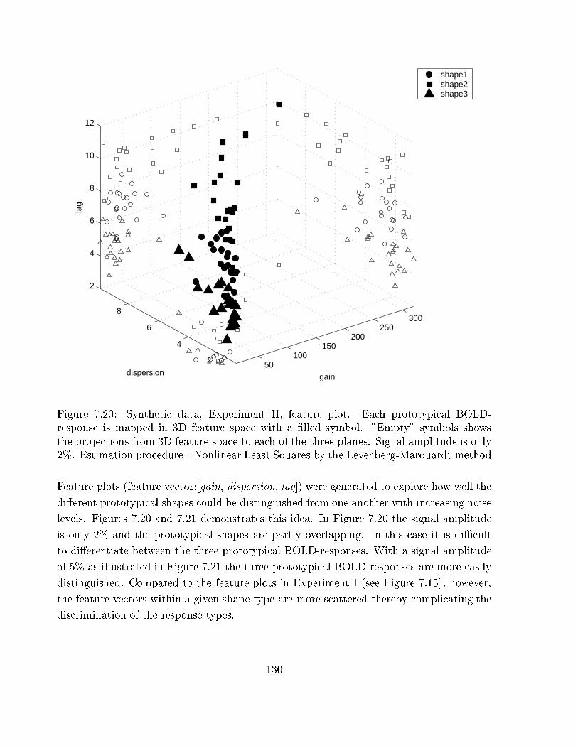
50100
150200
250300
2
4
6
8
2
4
6
8
10
12
gaindispersion
lag
shape1shape2shape3
Figure 7.20: Synthetic data, Experiment II, feature plot. Each prototypical BOLD-
response is mapped in 3D feature space with a �lled symbol. "Empty" symbols shows
the projections from 3D feature space to each of the three planes. Signal amplitude is only
2%. Estimation procedure : Nonlinear Least Squares by the Levenberg-Marquardt method
Feature plots (feature vector:[gain, dispersion, lag]) were generated to explore how well the
di�erent prototypical shapes could be distinguished from one another with increasing noise
levels. Figures 7.20 and 7.21 demonstrates this idea. In Figure 7.20 the signal amplitude
is only 2% and the prototypical shapes are partly overlapping. In this case it is diÆcult
to di�erentiate between the three prototypical BOLD-responses. With a signal amplitude
of 5% as illustrated in Figure 7.21 the three prototypical BOLD-responses are more easily
distinguished. Compared to the feature plots in Experiment I (see Figure 7.15), however,
the feature vectors within a given shape type are more scattered thereby complicating the
discrimination of the response types.
130

50100
150200
250300
2
4
6
8
2
4
6
8
10
12
gaindispersion
lag
shape1shape2shape3
Figure 7.21: Synthetic data, Experiment II, feature plot. Each prototypical BOLD-
response is mapped in 3D feature space with a �lled symbol. "Empty" symbols shows
the projections from 3D feature space to each of the three planes. Signal amplitude is 5%.
Estimation procedure : Nonlinear Least Squares by the Levenberg-Marquardt method
Since the Kruggel & Cramon Model incorporates spatial information as well as temporal
information, the high spatial correlation present in our synthetic data may explain the
large distortions of the prototypical BOLD-responses. The Nonlinear Least Squares Model
(Section 5.1) performs averaging over multiple trials, and ignores any spatial correlation
between voxels. For the present model, however, the e�ects of spatial correlation seemed
to yield poorer parameter estimates compared to the Nonlinear Least Squares Model.
131

7.1.5 Experiment: III Convolved Compartment Model
Experiments with the Convolved Compartment Model were performed on the same ROI
time series as those used for the experiments with the Kruggel & Cramon Model. All ROI
time series, each of which held 20 trials with 12 time points each, were modulated with
two di�erent prototypical BOLD-responses (shape 4 and 5, cfr. Section 7.1.2). Parameter
estimates were obtained separately for all trials in each of the 40 ROI time series. The
main intention for these experiments were
- to explore how well the model could approximate the prototypical BOLD-response,
and furthermore
- to obtain estimates of the neuronal parameters (gain, onset of neuronal response (t0)
and duration of neuronal response (t1)).
Due to the previously discussed diÆculties with regard to the vascular parameters of the
Convolved Compartment Model (see Section 6.5), we shall not attempt to interpret these
parameters.
Parameter estimation procedures included both the Nelder & Mead Downhill Simplex
Method and the Levenberg-Marquardt method. Preliminary experiments conveyed, how-
ever, that the better results were achieved using the Levenberg-Marquardt method. The
parameter estimates found with the Nelder & Mead Downhill Simplex Method were gen-
erally further from the true parameter values than the corresponding parameter estimates
found by the Levenberg-Marquardt method. Large departures from the true values also
occurred much more frequently with the Nelder & Mead Downhill Simplex Method. Fur-
thermore, there is a marked di�erence in computation times for the two algorithms, with
the Levenberg-Marquardt method being the fastest of the two. The main body of ex-
periments with the Convolved Compartment Model was therefore conducted using the
Levenberg-Marquardt method for parameter estimation. All results presented below have
been obtained with this method.
An example of a typical estimation result for the three neuronal parameters, gain, onset and
duration of neuronal activity (see Section 5.3), and for both prototypical BOLD-responses
is given in Table 7.4. Signal amplitude for this example is 4%. Neuronal onset times (t0)
were generally found to be below one second for prototypical BOLD-response, shape 4,
and below two seconds for shape 5 and neuronal duration times (t1) were in the range 2-6
seconds for shape 4 and in the range 6-10 seconds for shape 5. Gain was found between
5-13 AU (Arbitrary units) for shape 4 and 3-8 AU for shape 5.
132

Normality tests according to Lilliefors and Bera-Jarque (see Appendix A.4) in the residual
distributions after estimation were ful�lled for the majority of the regions.
Figure 7.22 shows the synthetic and modeled signals in eight consecutive trials for a typical
ROI time series. Signal amplitude is 4%. As the �gure illustrates, an acceptable �t could
not be achieved for all trials.
Shape 4 Shape 5
gain t0 t1 gain t0 t1
True 7.0000 0.0500 4.6000 4.0000 0.2500 8.0000
Estimated 8.7906 0.0758 4.4340 4.9816 0.3178 8.6862
" 8.6837 0.0665 4.1884 4.5545 0.0147 6.0147
" 6.9935 0.5322 5.4678 3.7049 1.3022 4.6978
" 7.8754 0.2912 5.8232 4.0973 0.0000 8.8289
Table 7.4: Synthetic data, Experiment III: Neuronal parameters (gain, onset (t0) and
duration (t1)). Results from 4 representative ROI's, prototypical BOLD-responses, shape
4 and 5, signal amplitude is 4%. Nonlinear Least Squares by the Levenberg-Marquardt
method.
0 10 20 30 40 50 60 70 80 90 100−15
−10
−5
0
5
10
15
20
25
30
Time points
Arbit
rary
unit
s
Model with estimated parametersSynt. signal in ROI
Figure 7.22: Synthetic data, Experiment III: Plot of synthesized (prototypical BOLD-
response, shape 5) and modeled signal in eight consecutive trials. Signal amplitude is
4%.
133

05
1015
2025
30
0
1
2
3
4
50
2
4
6
8
10
12
gain
onset of neuronal activation (t0)
du
rati
on
of
neu
ron
al a
ctiv
atio
n (
t1)
shape1shape2
Figure 7.23: Synthetic data, Experiment III, feature plot. Each prototypical BOLD-
response is mapped in 3D feature space with a �lled symbol. "Empty" symbols shows
the projections from 3D feature space to each of the three planes. Signal amplitude is 4%.
Estimation procedure: Nonlinear Least Squares by the Levenberg-Marquardt method
Feature plots were generated based on the three neuronal parameters (gain, onset (t0)
and duration (t1)). An example plot is shown in Figure 7.23. The two prototypical
BOLD-responses can relatively easily be distinguished from one another. However, most
BOLD-responses would be expected to appear with values somewhere in between the two
neuronal parameter sets used for the prototypical BOLD-responses of this experiment (see
Section 7.1.2). Especially the onset of neuronal activation cannot be expected to vary much
for di�erent BOLD-responses. These e�ects may reduce the power of the feature plots in
deriving the characteristics of the neuronal parameters of the Convolved Compartment
Model.
134

Our test results show that the Convolved Compartment Model is capable of approximat-
ing the two prototypical BOLD-responses used in our synthetic data. The Levenberg-
Marquardt method was found to yield better estimates (with less computation time) than
the Nelder & Mead Downhill Simplex Method. Neuronal parameters can be approximated
and was mapped in 3D feature space.
135

7.2 Real Data
7.2.1 Experiment: IV : Signal Detection
ANOVAs ability to detect activation was tested on a data set from an event-related ex-
periment performed at Haukeland University Hospital. The experiment was performed
on a Siemens Vision Plus 1.5 Tesla scanner equipped with 25mT/m gradients. 50 BOLD
sensitive Echo Planar Images (EPI, see Section 2.2.7) were acquired. Each measurement of
4 seconds consisted of 40 axial slices. Interscan interval was 6 seconds. With this temporal
resolution only 4 scans were recorded per trial. The time between successive trials was 24
seconds.
At each trial the subject was instructed to �nger-tap either with his right or left hand. Im-
ages were preprocessed and analyzed using the SPM software package (see Appendix A.3).
Figures 7.24 and 7.25 shows the corresponding activation plots. As could be expected, left
hand �nger tapping leads to activation in the motor cortex of the right hemisphere, and
visa versa for right hand �nger tapping.
The collected signals for each voxel time series were organized in two l � o matrices, in
which l is the number of time points per trial and o is the number of trials for each of the
two trial types. In this experiment there were 4 time points per trial and 5 trials per trial
type. Each voxel time series is organized such that there is one matrix for trial condition
left, and one for trial condition right hand �nger-tapping. The matrices are then subject
to the ANOVA procedure (see Section 4.1).
The entire data set was analyzed with the ANOVA procedure. The initial hypothesis states
that there is no signi�cant activation. Assessing the F-critical value with the corresponding
degrees of freedom (df), which for this experiment is dfnumerator=3 and dfdenominator = 16,
we �nd that the hypothesis can be rejected if F exceeds 9.00. This is the F critical value
at a 0.1% level, which means that 0.1% of reported activation may be erroneously.
The results from this analysis were then compared to the results from the SPM analysis.
Depending on the tresholding, all voxels labeled as activated by the SPM were also detected
by ANOVA. ANOVA generally yielded a moderately larger number of activated voxels than
the SPM. Basically, ANOVA compares several measures of the mean, and the null hypoth-
esis states that there are "no di�erence" in the means. Any time series with signi�cant
deviations from the mean may therefore be labeled as active. This makes ANOVA equally
good at detecting de-activations as activations. Normally, the results should therefore be
subject to further investigation/analysis.
136

BRAIN ACTIVATION MAP
TASK: LEFT HAND FINGER TAPPING
Figure 7.24: Real data, Experiment IV: activation plot. Trial type is left hand �nger
tapping.
BRAIN ACTIVATION MAP
TASK: RIGHT HAND FINGER TAPPING
Figure 7.25: Real data, Experiment IV: activation plot. Trial type is right hand �nger
tapping.
137

ANOVA makes no assumptions about the time course of the BOLD-response. The proce-
dure is therefore potentially capable of detecting responses with di�erent shapes across the
cortex. With the temporal resolution of the current experiment (4 observations per trial),
however, there is little chance of further investigating such di�erences.
An example matrix from a voxel in the left hemisphere, left hand �nger-tapping, is given
in Table 7.5.
Trial712 713 714 706 703
Time 711 717 709 712 704710 714 704 716 704704 705 712 711 707
Table 7.5: Real data, Experiment IV, ANOVA: Voxel values in a activated voxel in the left
hemisphere, left hand �nger tapping. The F-ratio is 0.3053 and the null-hypothesis is not
rejected
The F-value for the data in Table 7.5 was found to be 0.3053 and consequently the null
hypothesis cannot be rejected. This was expected since left hand �nger tapping basically
leads to activation in the right hemisphere. Table 7.6 gives an example of an activated voxel
in the right hemisphere, left hand �nger tapping. The F-ratio for this voxel is 21.0648
and clearly indicates that the null hypothesis should be rejected. Figure 7.26 gives an
illustration of the corresponding time courses.
Trial706 718 713 714 712
Time 729 727 718 730 723709 706 709 715 708700 704 703 699 712
Table 7.6: Real data,Experiment IV, ANOVA: Voxel values in a activated voxel in the left
hemisphere (same voxel as in table 7.5, right hand �nger tapping. The F-ratio is 21.0648
and the null-hypothesis is rejected at the 0.1% level.
138

1 2 3 4
690
695
700
705
710
715
720
725
730
735
740
scan
Arb. u
nits
Voxel in left hemisphere: Right hand fingertapping
1 2 3 4
690
695
700
705
710
715
720
725
730
735
740
scan
Arb. u
nits
Voxel in left hemisphere: Left hand fingertapping
Figure 7.26: Real data, Experiment IV, time course for voxel in motor cortex of the left
hemisphere, (a) right hand �nger tapping, and (b) left hand �nger tapping.
139

7.2.2 Experiment V : Signal Description
The fMRI dataset employed in this experiment was obtained for a language comprehension
study. On a Siemens Vision Plus 1.5 Tesla scanner at Haukeland University Hospital, 501
echo-planar images (EPI, see Section 2.2.7) were collected (TE = 60ms, TR=0.6ms, ip
angle 90Æ, FOV 200�200 mm, scan time 2 sec). Each volume consists of 20 slices of 64�64
voxels and a spatial resolution 3.13�3.13�4 mm. A corresponding anatomical image (3D
FLASH, see Section 2.2.7) was acquired in the same session.
While in the scanner, Norwegian words versus non-words were presented randomly inter-
mixed, to the subject on a visual display. The stimuli were presented with inter-stimulus
interval ranging from 1-14 seconds. The subject was to respond to a word by pressing a
right hand button, and to a non-word by pressing a left hand button.
The dataset was preprocessed and analyzed with the SPM99 software package (see Ap-
pendix A.3). Figures 7.27 and 7.28 illustrates the location of activated areas for trial
types non-word and word, respectively. In locating areas of activation suitable for the sig-
nal description problem, the voxel time series for the activated areas were �rst subject to
visual inspection. To reduce the e�ect of summation of closely spaced trials, only trials
in which a word was followed by a non-word and visa versa, were selected for further in-
vestigations. Furthermore, trials with "long" inter-stimulus intervals (8-12 seconds) were
chosen.
A total of 7 di�erent ROI time series were chosen, 4 ROI time series for trial type word and
three ROI time series for trial type non-word. In these ROI time series a total of 18 trials
were selected for the experiments to follow. Baseline correction was performed separately
for all voxels. Each trial is represented by a ROI of nine voxels in a 3�3 voxel grid and
12 time points. Activation were found to be in the order �2-4% relative to mean signal
intensity level.
140

BRAIN ACTIVATION MAP
TRIAL TYPE : NONWORD
Figure 7.27: Real data, Experiment V: activation plot. Trial type non-word.
BRAIN ACTIVATION MAP
TRIAL TYPE : WORD
Figure 7.28: Real data, Experiment V: activation plot. Trial type word.
141
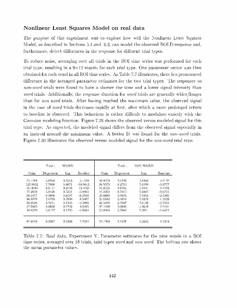
Nonlinear Least Squares Model on real data
The purpose of this experiment was to explore how well the Nonlinear Least Squares
Model, as described in Sections 5.1 and 6.3, can model the observed BOLD-response and,
furthermore, detect di�erences in the response for di�erent trial types.
To reduce noise, averaging over all trials in the ROI time series was performed for each
trial type, resulting in a 9�12 matrix for each trial type. One parameter vector was then
obtained for each voxel in all ROI time series. As Table 7.7 illustrates, there is a pronounced
di�erence in the averaged parameter estimates for the two trial types. The responses to
non-word trials were found to have a shorter rise time and a lower signal intensity than
word trials. Additionally, the response duration for word trials are generally wider/longer
than for non-word trials. After having reached the maximum value, the observed signal
in the case of word trials decreases rapidly at �rst, after which a more prolonged return
to baseline is observed. This behaviour is rather diÆcult to modulate exactly with the
Gaussian modeling function. Figure 7.29 shows the observed versus modeled signal for this
trial type. As expected, the modeled signal di�ers from the observed signal especially in
an interval around the maximum value. A better �t was found for the non-word trials.
Figure 7.30 illustrates the observed versus modeled signal for the non-word trial type.
Trial : WORD Trial : NON-WORD
Gain Dispersion Lag Baseline Gain Dispersion Lag Baseline
71.4789 5.6356 9.3513 -5.4529 46.9579 3.8239 7.8306 -4.2432
121.9622 7.7006 9.8671 -10.0641 38.5573 3.2713 7.6399 -3.4777
164.8185 8.9174 9.9756 -13.4761 25.8756 2.6165 7.4444 -2.1123
77.2050 5.8426 9.5321 -5.9962 44.3202 3.7315 7.6907 -3.6745
98.1077 6.9066 9.8297 -8.2650 35.0486 3.0951 7.5361 -2.7382
96.3070 7.0793 9.7886 -8.5887 25.5332 2.5856 7.4272 -1.7522
56.9126 4.9414 9.1135 -4.3880 36.3496 3.5507 7.6146 -2.7151
52.9905 4.9850 9.2223 -4.5205 32.1598 3.0040 7.4678 -2.2407
48.6270 5.0177 9.1735 -4.5024 24.9860 2.7060 7.4654 -1.6274
87.6010 6.3362 9.5393 -7.2504 34.4209 3.1538 7.5685 -2.7313
Table 7.7: Real data, Experiment V. Parameter estimates for the nine voxels in a ROI
time series, averaged over 18 trials, trial types word and non-word. The bottom row shows
the mean parameter values.
142

0 10 20 30−5
0
5
10Voxel : 1
0 10 20 30−10
−5
0
5
10Voxel : 2
0 10 20 30−10
−5
0
5
10Voxel : 3
0 10 20 30−5
0
5
10Voxel : 4
0 10 20 30−10
−5
0
5
10Voxel : 5
0 10 20 30−10
−5
0
5
10Voxel : 6
0 10 20 30−5
0
5
10Voxel : 7
0 10 20 30−5
0
5
10Voxel : 8
0 10 20 30−5
0
5
10Voxel : 9
averaged signalmodel
Figure 7.29: Real data, Experiment V, word versus non-word discrimination task. Param-
eter estimates for a ROI time series averaged over 18 trials, trial type: word. Time-locked
to stimulus averaging of observed time course over all trials is denoted by star dots. The
estimated model signal time course is denoted by solid line.
Figure 7.31 shows plots of single trials and the corresponding modeled signal constructed
from the averaged parameter sets (cfr. Table 7.7). In Figure 7.32 the modeled signals for
trial types word versus non-word can be visually compared. The di�erences between the
two types of responses are clearly demonstrated.
QQ-plots were generated for a visual inspection of normality in the residuals. All plots
conveyed residual distributions in good accordance with normality. An example plot is
given in Figure 7.33, in which the residual distribution for trial type non-word is plotted
versus a normal distribution. Normality tests according to Lilliefors and Bera-Jarque (see
Appendix A.4) con�rmed normality in all residuals for both trial types.
143

0 10 20 30−10
−5
0
5
10Voxel : 1
0 10 20 30−5
0
5
10Voxel : 2
0 10 20 30−5
0
5
10Voxel : 3
0 10 20 30−5
0
5
10Voxel : 4
0 10 20 30−5
0
5
10Voxel : 5
0 10 20 30−5
0
5
10Voxel : 6
0 10 20 30−5
0
5
10Voxel : 7
0 10 20 30−5
0
5
10Voxel : 8
0 10 20 30−5
0
5
10Voxel : 9
averaged signalmodel
Figure 7.30: Real data, Experiment V, word versus non-word discrimination task. Results
from estimation, averaged over 18 trials, trial type: non-word. Time-locked to stimulus
averaging of observed time course over all trials is denoted by star dots. The estimated
model signal time course is denoted by solid line.
The feature plot (see Figure 7.34) maps the estimated parameters gain(�0), dispersion(�1)
and lag(�2) in 3D feature space. non-word trial characteristics can easily be identi�ed.
word trial characteristics are, however, more scattered but clearly (linearly) separable from
non-word trials. To our knowledge, these �ndings in haemodynamic response features have
not been reported before. However, data are sparse, just one er-fMRI experiment, and
should be con�rmed by a more extensive experimental study.
144

0 2 4 6 8 10 12 14 16 18 20 22−15
−10
−5
0
5
10
15
20
seconds
arb.
units
0 2 4 6 8 10 12 14 16 18 20 22−10
−5
0
5
10
15
20
seconds
arb.
units
WORD NON−WORD
lag ~ 7.5 sec lag ~ 9.5 sec
dispersion ~ 6.3 dispersion ~ 3.1
(a) (b)
Figure 7.31: Real data, Experiment V, word versus non-word discrimination task, Nonlinear
Least Squares Model: Plot of single trials (dotted lines) and averaged modeled signal (solid
line). (a) Trial type word: "Height" of response is given by �0=�1 � 87:6=6:3 = 13:9
which yields a maximum value of 6.6 (baseline + �0=�1). This value is reached after
approximately 7.5 seconds (lag). (b) Trial type non-word: "Height" of response is given by
�0=�1 � 34:4=3:1 = 10:9 which yields a maximum value of 8.2 (baseline + �0=�1). This value
is reached after approximately 9.5 seconds (lag). (cfr. Table 7.7 for the exact averaged
parameter values.)
0 1 2 3 4 5 6 7 8 9 10 11 12 13 14 15 16 17 18 19 20 21 22−6
−4
−2
0
2
4
6
8
10
seconds
arb.
units
lag ~ 7.5 sec
lag ~ 9.5 sec
non−word
word
Modeled signals (word versus non−word)
Figure 7.32: Real data, Experiment V, word versus non-word discrimination task, Nonlinear
Least Squares Model: Signals constructed from averaged parameter estimates for the two
trial types. (cfr. Table 7.7 for the exact averaged parameter values.)
145

−2 0 2−4
−2
0
2
4
Qua
ntile
s of
Inpu
t Sam
ple Voxel 1
−2 0 2−4
−2
0
2
4
Qua
ntile
s of
Inpu
t Sam
ple Voxel 2
−2 0 2−4
−2
0
2
4
Qua
ntile
s of
Inpu
t Sam
ple Voxel 3
−2 0 2−5
0
5
Qua
ntile
s of
Inpu
t Sam
ple Voxel 4
−2 0 2−4
−2
0
2
4
Qua
ntile
s of
Inpu
t Sam
ple Voxel 5
−2 0 2−4
−2
0
2
4
Qua
ntile
s of
Inpu
t Sam
ple Voxel 6
−2 0 2−5
0
5
Qua
ntile
s of
Inpu
t Sam
ple Voxel 7
Standard Normal Quantiles−2 0 2
−4
−2
0
2
4
Qua
ntile
s of
Inpu
t Sam
ple Voxel 8
Standard Normal Quantiles−2 0 2
−4
−2
0
2
4
Qua
ntile
s of
Inpu
t Sam
ple Voxel 9
Standard Normal Quantiles
Figure 7.33: Real data, Experiment V, word versus non-word discrimination task. QQ
Plot of Sample Data residual, averaged over 18 trials, versus Standard Normal. Trial type:
non-word.
4060
80100
120140
160
34
56
78
2
4
6
8
10
12
gaindispersion
lag
word nonword
Figure 7.34: Real data, Experiment II word versus non-word discrimination task: feature
plot. Each trial type is mapped in 3D feature space with a �lled symbol. "Empty" symbols
shows the projections from 3D feature space to each of the three planes.
146

Kruggel & Cramon Model on real data
The Kruggel & Cramon Model estimates one separate parameter set for each trial in a
ROI time series. For the current dataset, 36 trials from 7 ROI time series were selected
for further investigations. In some of the trials, especially with a low Signal to Noise Ratio
(SNR, see Section 2.2.8), the BOLD-responses were severely distorted or too deviant in the
sample region to warrant a good �t. The largest deviations were found with the trial type
word. In approximately 30% of the trials the model failed to achieve a satisfying adaption
to the sampled fMRI signal. Averaged parameter estimates for the remaining trials in all
ROI's can be found in Table 7.8.
Example plots from two di�erent ROI time series are presented in Figures 7.35 and 7.36.
The feature plot in Figure 7.37 con�rms that the largest departures from the mean is seen
for trial type word. For the non-word trial type, parameter characteristics can to some
extent be determined, whereas for the word trial type no such conclusions can be drawn.
Normality tests according to Lilliefors and Bera-Jarque(see Appendix A.4) con�rmed nor-
mality in all residuals for both trial types.
Trial : WORD Trial : NON-WORD
Gain Dispersion Lag Baseline Gain Dispersion Lag Baseline
36.7180 2.7870 7.5791 -2.8746 35.3099 2.9224 7.0675 -6.8290
141.1739 9.0585 13.0306 -10.6258 46.6619 3.6117 5.6928 -3.8845
24.7125 3.4014 9.2410 -1.7730 23.8989 2.9400 7.4773 -0.1459
307.0840 13.9128 11.1069 -19.5104 24.5346 1.3925 6.9339 -4.0164
11.8436 0.7712 6.9187 -2.3905 92.8113 3.9233 7.2863 -8.7572
143.6619 6.0329 8.8314 -12.0236 18.5327 2.6634 9.1248 -1.6461
36.9821 4.1456 6.0373 -5.0625 17.0727 2.0756 5.2713 4.4137
51.0206 3.8475 5.0568 -7.5863 25.9019 2.3142 8.3210 -0.3818
28.5196 0.4991 8.8485 4.3434 26.6279 3.3094 6.6119 -4.6454
10.5259 3.2079 6.5549 -2.3878 40.7389 0.4324 9.0343 -1.0107
57.8554 33.8455 15.9449 -2.8446 22.1474 2.0190 8.2904 0.0726
24.4007 2.2089 7.0327 -5.2576
15.4340 2.5000 8.9578 -1.4843
61.6032 2.9931 6.9350 -4.8931
65.3580 5.3831 7.8529 -6.2393
Mean Parameter Values
77.2816 7.4099 9.0136 -5.7033 36.0689 2.7126 7.4593 -2.9803
Table 7.8: Real data, Experiment V, word versus non-word discrimination task, Kruggel
& Cramon Model. Parameter estimates for trial types word (11 ROI's) and non-word
(15 ROI's). The bottom row shows the mean parameter values for trial type word versus
non-word.
147
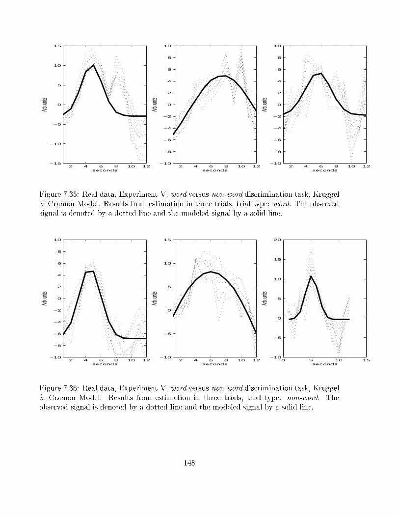
2 4 6 8 10 12−15
−10
−5
0
5
10
15
seconds
Arb. un
its
2 4 6 8 10 12−10
−8
−6
−4
−2
0
2
4
6
8
10
seconds
Arb. un
its
2 4 6 8 10 12−10
−8
−6
−4
−2
0
2
4
6
8
10
seconds
Arb. un
its
Figure 7.35: Real data, Experiment V, word versus non-word discrimination task, Kruggel
& Cramon Model. Results from estimation in three trials, trial type: word. The observed
signal is denoted by a dotted line and the modeled signal by a solid line.
2 4 6 8 10 12−10
−8
−6
−4
−2
0
2
4
6
8
10
seconds
Arb. un
its
2 4 6 8 10 12−10
−5
0
5
10
15
seconds
Arb. un
its
0 5 10 15−10
−5
0
5
10
15
20
seconds
Arb. un
its
Figure 7.36: Real data, Experiment V, word versus non-word discrimination task, Kruggel
& Cramon Model. Results from estimation in three trials, trial type: non-word. The
observed signal is denoted by a dotted line and the modeled signal by a solid line.
148

50100
150200
250300
510
1520
2530
2
4
6
8
10
12
gaindispersion
lag
WORD NON−WORD
Figure 7.37: Real data, Experiment V, word versus non-word discrimination task, Kruggel
& Cramon Model: feature plot. Each trial type is mapped in 3D feature space with a
�lled symbol. "Empty" symbols shows the projections from 3D feature space to each of
the three planes.
Our test results suggests that the approach taken in the Kruggel & CramonModel are not as
suitable for describing the observed BOLD-response as the approach taken in the Nonlinear
Least Squares Model. The responses approximated by the Kruggel & Cramon Model for
the two trial types, especially for the word trial type, cannot readily be characterized. A
high spatial correlation was revealed in the fMRI data set of this experiment. For the
spatial pattern illustrated in Figure 7.4, correlation coeÆcients in the x and y-directions
(see Section 5.2) were calculated to be in the range 0.95-1.0 for preprocessed and smoothed
data. In the Nonlinear Least Squares Model averaging for each trial type was performed
over 18 trials. The high spatial correlation found in the data and the fact that estimation
in the Kruggel & Cramon Model is performed over only nine trials (from the nine voxels
in a ROI) may explain some of the di�erence in results between the two models.
149

Chapter 8
Discussion and Conclusion
This work considers methods for the detection and description of stimulus induced brain
activation in er-fMRI. The emphasis has been on methods for characterization of the evoked
responses.
The chosen thesis subject is not only concerned with informatics, but deals also essentially
with image processing, brain physiology, cognitive neuroscience, neuroradiology and as-
pects of MRI instrumentation and acquisition. Therefore, the work has evidently been an
interdisciplinary enterprise. In evaluating the methods being described the aim was not
only to consider issues related to mathematical modeling, but also an attempt to establish
physiological interpretations of the model parameters. Physiological aspects are impor-
tant both for the selection and evaluation of modeling functions. Parameters which are
physiologically interpretable descriptors of the BOLD-response can readily be applied in
multivariate analysis for comparison of for example duration of activation, reaction times
and e�ects of learning, aging and di�erent disease states.
The signal detection problem has been demonstrated with the ANOVA procedure, which
basically locate activated regions by comparing estimates of the mean for all trials of
the same type in a particular voxel. The signal description problem have been assessed
on the basis of three models, the Nonlinear Least Squares Model and the Kruggel &
Cramon Model, which both use a Gaussian function for the HRF, and the Convolved
Compartment Model, in which the modeling function integrates both neuronal and vascular
parameters. The fact that the neurovascular mechanisms behind the BOLD response is not
well understood lead to models based on di�erent physiological interpretations. In this work
two such di�erent models, the Convolved Compartment Model and the BalloonModel, have
been described, with experimental work limited to the Convolved Compartment Model.
Most datasets acquired at Haukeland University Hospital have a sampling frequency of 4-8
150

time points (i.e brain volume acquisitions) per trial. These datasets are therefore not the
best for the signal description problem. Due to the time limit on this work and the extensive
resources needed in design, recording and analysis (signal detection) of fMRI experiments,
we were only able to obtain one data set with a larger number of time steps per trial.
This data set, based on a dichotic listening paradigm which was under construction, was
described in Section 6.1. However, due to very low activation levels these data were not
used in the signal description experiments.
Evaluation of the experimental results depends on whether the data are synthetic or real.
For the synthetic data sets (observed fMRI time courses modulated with surrogate HRF
functions), true parameters can be established prior to estimation procedures. Upon com-
pletion of the experiments the estimated parameters can be compared with the true pa-
rameters. Evaluation of results for the real data sets are somewhat more involved. Due
to the lack of physiological experimental evidence these experiments should be regarded
more as a feasibility study. However, results with our data were encouraging (especially
on the word, non-word discrimination task) and follow-up studies of the signal description
problem should therefore be conducted with better er-fMRI data, using carefully designed
paradigms.
The main results can be summarized as follows:
Signal Detection using ANOVA
ANOVAs ability to detect activations have been tested on a real data set from an event-
related fMRI experiment performed at Haukeland University Hospital. For comparison the
data were also analyzed with the SPM software package (see Appendix A.3). We found
that ANOVA and SPM detected voxel activation in the same brain regions. ANOVA,
however, generally yielded a moderately larger number of activated voxels than the SPM,
and the results should therefore be regarded as a starting point for further investigation.
Signal Description with the Nonlinear Least Squares Model
� A Gaussian function (see Equation (3.6)) was used in the modeling of the BOLD-
response
� Noise reduction was performed by averaging over multiple trials time-locked to stim-
ulus
151

� Parameter estimates were obtained with Nonlinear Least Squares by the Gauss-
Newton method
� One set of parameters was estimated per voxel in all ROI time series
Experiments were performed on both synthetic and real data. The experimental results
demonstrate that this model is stable against noise levels commonly observed in fMRI
data. Considering the relatively high level of noise in our data, the parameter estimates
for the synthetic data set are found to be highly satisfactory. Feature plots demonstrated
that the three di�erent prototypical BOLD-responses employed in this experiment could
easily be distinguished even with signal amplitudes of only 2% relative to mean signal
intensity level. For the experiments on real data, we were able to characterize di�erential
responses in a word versus non-word discrimination task. Responses to non-word trials
were found to have a shorter rise time and duration as well as a lower signal intensity than
word trials (Figure 7.32). These results were illustrated in a feature plot of word versus
non-word (Figure 7.34). To our knowledge, these �ndings in estimated haemodynamic
response features in a word versus non-word discrimination task have not previously been
reported.
Signal Description with the Kruggel & Cramon Model
� The Gaussian function (see Equation (3.6)) was used in the modeling of the BOLD-
response
� Noise was collectively modeled in a covariance matrix and the temporal and/or spa-
tial correlations in the residuals were applied as weights in a weighted least squares
approach
� Parameter estimation was performed by the Levenberg-Marquardt method and/or
the Nelder & Mead downhill simplex method
� One set of parameter estimates was obtained per ROI
Results from the experiments on synthetic and real data were not as good as in the Non-
linear Least Squares Model, especially for the real data experiments. This model was also
less robust in cases of low SNR (see Section 2.2.8). This was illustrated by plots in 3D
feature space in which the three di�erent prototypical BOLD-responses could easily be
distinguished at a signal amplitude of 5%. With a signal amplitude of only 2%, however,
the BOLD-responses could not be separated. Reasons for these diÆculties may be found in
152

the high spatial correlation observed in our fMRI data sets. The Nonlinear Least Squares
Model (Section 5.1) incorporates averaging over multiple trials ignoring any spatial cor-
relation between voxels. For the Kruggel & Cramon Model, however, the high spatial
correlation and the fact that the estimation of each parameter set is performed over only
nine voxels (nine voxels in a ROI), are probable causes for the poorer parameter estimates.
The Levenberg-Marquardt method was favored for the parameter estimation of the model
concerned. We found this estimation procedure less likely to yield large departures from
the true parameter values than the Nelder & Mead Downhill simplex method. Moreover,
it was also approximately two times faster than the Nelder & Mead Downhill simplex
method.
Signal Description with the Convolved Compartment Model
� A physiologically motivated response function (see Section 5.3), involving both "neu-
ronal" and "vascular" parameters, was used in the modeling of the BOLD-response
� Noise was collectively modeled in a covariance matrix and the temporal and/or spa-
tial correlations in the residuals were applied as weights in a weighted least squares
approach
� Parameter estimation was performed by the Levenberg-Marquardt method and/or
the Nelder & Mead downhill simplex method
� One set of parameter estimates was obtained per trial per ROI
In the initial evaluation of this model we found that two signals that per de�nition (see
Section 6.5) were equal could be constructed from a number of relatively di�erent parameter
sets. Our test suggests that the landscape of the function to minimize (Equation (5.24)) is
rather shallow for the vascular parameters. This may lead to similar sub-optimal solutions
in a relatively wide parameter range. The uncertainty which arise from the high noise
levels in fMRI data and the relatively few time points per trial may therefore in uence
the probability of multiple solutions (many local minima). It seems possible to give a
physiological explanation, based on the dynamic relationship between the vascular transfer
rates, of this phenomenon. Robust parameter estimates for the Convolved Compartment
Model requires a large number of time points per trial. Therefore, the present rate at
which time points can be sampled in er-fMRI experiments limits the performance of the
Convolved Compartment Model. Consequently, only experiments on synthetic data were
carried out. Using di�erent pulse sequences (e.g Spin Echo and Gradient Echo EPI), which
have their maximum sensitivity to speci�c aspects of the microvasculature [2], it could to
153

some degree be possible to obtain experimental evidence for the separation of "neuronal"
and "vascular" parameters.
Our experiments with the Convolved Compartment Model con�rmed the model's ability
to approximate the prototypical BOLD-response and that neuronal response information
can be derived from the (neuronal) parameters. As with the Kruggel & Cramon Model,
the Levenberg-Marquardt method was less likely to yield large departures from the true
parameter values than the Nelder & Mead Downhill simplex method. This estimation
procedure was therefore also favored for the Convolved Compartment Model.
Main conclusions
� Simple averaging of time-locked to stimulus single trials combined with Nonlinear
Least Squares estimation of model parameters have been found to be well suited for
evaluating event-related fMRI data in terms of physiologically interpretable param-
eters.
� The Nelder & Mead Downhill Simplex Method has been suggested for the estimation
of the physiological parameters in the Kruggel & Cramon Model [27]. We have
successfully applied the Levenberg Marquardt Method for the parameter estimation
thereby reducing computation times approximately with a factor of two per ROI.
� Our experience with the Convolved Compartment Model was not as successful as
the two other signal description models. The main limitation for this model seems
to be the insuÆcient number of observations that can be collected per trial with the
currently available fMRI equipment. Our results imply that the model is stated more
as a feasibility study than a "new method to evaluate the BOLD-response". This
was also con�rmed by Dr.Frithjof Kruggel at the Max Planck Institute of Cognitive
Neuroscience (personal communication).
� Regarding physiological interpretations of the estimated parameters we selected three
parameter estimates to be plotted in 3D feature space. This plot can potentially
indicate if the joint distribution of the selected parameters are suÆciently separated to
discriminate between di�erent types of BOLD-responses. Feature plots may thus give
information about underlying neuronal processing mechanisms. For the Nonlinear
Least Squares Model and the Kruggel & Cramon Model we selected the parameters
lag, dispersion and gain (which might express neuronal processing delay, processing
duration or asynchrony and processing strength, respectively).
154
The main idea of extracting parameter feature vectors from the single trial responses
depicted in feature plots (e.g. Figures 7.14 and 7.15) was to bring our estimation of
physiologically interpretable parameter into a statistical classi�cation framework. By
statistical classi�cation of di�erent haemodynamic response types (shapes) it would
be possible to distinguish and characterize neural information processing in di�erent
brain locations during a given paradigm. Each classi�ed response could then give
information about processing delay, number of neurons in the �ring population and
duration/asynchrony of �ring at that particular brain location, and thus yield more
information about functional anatomy than simple activation detection. We found
that these plots are well suited for investigating di�erent types of BOLD-responses.
For visualization and easier interpretation, the di�erent BOLD responses can be
labeled and mapped to the corresponding anatomical images. To our knowledge
�ndings in haemodynamic response features related to a word versus non-word dis-
crimination task, as described in this work, have not been reported elsewhere. Such
feature classi�cation studies could therefore be an interesting follow up of the present
signal description and estimation study.
155

Appendix A
Appendix
A.1 The convolution operator ?
In the signal processing litterature the symbol ? is used for convolution, mixed convolution,
and discrete convolution.
In case of f; g : R 7! R, the convolution f ? g is de�ned as
(f ? g)(t) =
Z1
�1
f(�)g(t� �) d� t 2 R (A.1)
If b = fbkgk2Z is a discrete sampled signal (i.e. a sequence) we de�ne the mixed convo-
lution b ? f as
(b ? f)(t) =
1Xk=�1
b(k)f(t� k) t 2 R (A.2)
If a = fakgk2Z and b = fbkgk2Z are discrete sampled signals, we de�ne the discrete
convolution a ? b as
(a ? b)(m) =
1Xk=�1
a(k)b(m� k) m 2 Z (A.3)
In all cases we assume f; g 2 L2(R), i.e. f and g are square-integrable real functions, and
a; b 2 l2, i.e. a and b are square-summable discrete signals.
A.2 Fisher distribution
The F-distribution is given by
h(F ) =�(v1+v2
2)
�(v12) �(v2
2)(v1
v2)v12
Fv1�2
2
(1 + Fv1v2)v1+v2
2
156

where v1 is the number of points per trial minus one, and v2 is the total number of data
points minus the number of points per trial. � is the gamma function in which
�(v) =
Z +1
0
ettv�1
dt:
The F-distribution with various degrees of freedom in numerator and denominator is illus-
trated in Figure A.1.
0 1 2 3 4 5 6 7 8 90
0.2
0.4
0.6
0.8
1
1.2
1.4Plots of the distribution of F−scores
F−score
arb.
uni
ts
d.f = 3,16, 0.1 percent critical point = 9.00 d.f = 8,12, 0.1 percent critical point = 7.71 d.f = 40,40, 0.1 percent critical point = 2.73
Figure A.1: F-distribution with various degrees of freedom in numerator and denominator.
The 0.1% critical point (beyond which the null hypothesis is rejected) moves towards 1 as
the degrees of freedom increase.
A.3 SPM99
The SPM (Statistical Parametric Mapping) software package is a suite of Matlab functions
and subroutines (with some externally compiled C routines) which organizes and interprets
functional neuroimaging data. Main features of the software are:
- Realignment of image sequences
- Automated non-linear spatial normalisation
- Image segmentation
157

- Coregistration
- Spatial smoothing
- Formation of statistic images
- Assessment of Statistic Images
- Interrogation of results (plots, local maxima, overlaying of statistical results onto
structural images)
- Global adjustment and image averaging
Further information can be found at the SPM website: www.�l.ion.ucl.ac.uk/spm
A.4 Matlab functions [31]
� chol
Cholesky factorization. chol(X) uses only the diagonal and upper triangle of X. The
lower triangular is assumed to be the (complex conjugate) transpose of the upper.
If X is positive de�nite, then R = CHOL(X) produces an upper triangular R so that
R0
�R = X. If X is not positive de�nite, an error message is printed.
� fminsearch
Multi-dimensional unconstrained nonlinear minimization by Nelder & Mead downhill
simplex method. Given an initial starting parameter vector fminsearch �nds the
minimum of a scalar function of several parameters. X = fminsearch(FUN, X0,
OPTIONS, P1, P2,...) returns a vector X that is a local minimizer of the function
that is described in FUN near the starting vector X0. FUN should return a scalar
function value when called with feval: F=feval(FUN,X). Optimization parameters
are speci�ed in the structure OPTIONS. Default values are used if an empty matrix
is given for OPTIONS . P1,P2,... provides for additional arguments which are passed
to the objective function, F=feval(FUN,X,P1,P2,...).
� jbtest
The Bera-Jarque test evaluates the hypothesis that X has a normal distribution
with unspeci�ed mean and variance, against the alternative that X does not have a
normal distribution. The test is based on the sample skewness and kurtosis ofX. The
Jarque-Bera test is an asymptotic test, and should not be used with small samples.
H = jbtest(X,ALPHA) determines if the null hypothesis of composite normality is a
158

reasonable assumption regarding the population distribution of a random sample X.
The desired signi�cance level, ALPHA, is an optional scalar input (default = 0.05).
H indicates the Boolean result of the hypothesis test:
{ H = 0 ) Do not reject the null hypothesis at signi�cance level ALPHA.
{ H = 1 ) Reject the null hypothesis at signi�cance level ALPHA.
� kron Kronecker product. kron (X,Y) is the Kronecker product of X and Y . The
result is a large matrix formed by taking all possible products between the elements
of X and those of Y .
� lillietest
The Lilliefors test evaluates the hypothesis that X has a normal distribution with
unspeci�ed mean and variance, against the alternative that X does not have a nor-
mal distribution. This test compares the empirical distribution of X with a nor-
mal distribution having the same mean and variance as X. It is similar to the
Kolmogorov-Smirnov test, but it adjusts for the fact that the parameters of the nor-
mal distribution are estimated from X rather than speci�ed in advance. [H,P] =
lillietest(X,ALPHA) determines if the null hypothesis of composite normality is a
reasonable assumption regarding the population distribution of a random sample X.
The desired signi�cance level, ALPHA, is an optional scalar input (default = 0.05).
H indicates the result of the hypothesis test:
{ H = 0 ) Do not reject the null hypothesis at signi�cance level ALPHA.
{ H = 1 ) Reject the null hypothesis at signi�cance level ALPHA.
P is computed via interpolation into the Lilliefors simulation table. A NaN is returned
when P is not found within the interval 0.01 � P � 0.20.
� lsqnonlin
Solves nonlinear least squares problems, including nonlinear data-�tting problems of
the form minfP
x FUN(X)2g where X and the values returned by FUN can be vec-
tors or matrices. [X, RESNORM, RESIDUAL, EXITFLAG, OUTPUT] = lsqnonlin(FUN,
X0, LB, UB, OPTIONS, P1, P2,..) starts at the matrix X0 and �nds a minimum
X to the sum of squares of the functions in FUN. LB and UB de�nes a set of lower
and upper bounds on the design parameters, X, so that the solution is in the range
LB � X � UB. Optimization parameters are speci�ed in the structure OPTIONS.
Default values are used if an empty matrix is given for OPTIONS. P1,P2,... are
159
problem-dependent parameters and are passed directly to the function FUN(X, P1,
P2,...). RESNORM is the value of the squared 2-norm of the residual atX. RESID-
UAL is the value of the residual at the solution X. EXITFLAG describes the exit
condition of LSQNONLIN:
{ EXITFLAG > 0 : LSQNONLIN converged to a solution X
{ EXITFLAG = 0 : the maximum number of function evaluations was reached.
{ EXITFLAG < 0 : LSQNONLIN did not converge to a solution.
The structure OUTPUT returns the number of iterations taken in OUTPUT.iterations,
the number of function evaluations in OUTPUT.funcCount and the algorithm used
in OUTPUT.algorithm.
� nlinfit
Nonlinear least-squares data �tting by the Gauss-Newton method. nlinfit(t,
g, 'MODEL', theta0) �nds the coeÆcients of the nonlinear function described in
MODEL. MODEL is a user supplied function having the form g = fun(theta,t).
That is MODEL returns the predicted values of ggiven initial parameter estimates,
beta, and the independent variable, t. [theta, res, jac] = nlinfit(t, g, 'MODEL',
theta0) returns the �tted coeÆcients theta, the residuals, res, and the Jacobian ma-
trix, jac, at the solution.
� nlparci
Computes con�dence intervals on parameters of nonlinear models. ci = nlparci(X,
res, jac) returns the 95% con�dence interval ci on the nonlinear least squares
parameter estimate X, given the residual sum of squares, res, and the Jacobian
matrix ,jac, at the solution. The con�dence interval calculation is valid for systems
where the number of rows of J exceeds the length of X.
160

A.5 Frequently used Abbreviations
2D,3D fone, two, threeg-dimensional
ANOVA ANalysis Of VAriance
BOLD Blood Oxygenation Level Dependent
Dispersion Duration of BOLD-response
EPI Echo Planar Imaging
er-fMRI event-related functional Magnetic Resonance Imaging
FLASH Fast Low-Angle SHot
fMRI functional Magnetic Resonance Imaging
FOV Field of View
Gain Gain/strength of BOLD response / number of neurons in �ring population
HRF Haemodynamic Response Function
Lag Time to peak / maximum intensity of BOLD response
LM Levenberg-Marquardt Method
MRI Magnetic Resonance Imaging
NM Nelder & Mead downhill simplex method
Pixel Picture Element
ROI Region Of Intrest
SNR Signal to Noise Ratio
SPM Statistical Parametric Mapping (see Appendix A.3)
TE Echo Time
TR Repetition Time
Voxel Volume element
161

Bibliography
[1] J. Ashburner and K. J. Friston. Image Registration, chapter 26, pages 285{299. In [35], 1999.
[2] P. A. Bandettini. The Temporal Resolution of Functional MRI, chapter 19, pages 205{220. In [35],
1999.
[3] J. Belliveau, D. N. Kennedy, R. C. McKinstry, B. R. Buchbinder, R. M. Weissko�, M. Cohen, J. M.
Vevea, T. J. Brady, and B. R. Rosen. Functional mapping of the human visual cortex by magnetic
resonance imaging. Science, 254:716{719, 1991.
[4] F. Bloch. Nuclear induction. The Physical Review, 70:460{474, 1946.
[5] G. M. Boynton, S. A. Engel, G. H. Glover, and D. J. Heeger. Linear systems analysis of functional
magnetic resonance imaging in human v1. The Journal of Neuroscience, 16:4207{4221, 1996.
[6] R. L. Buckner. Event-related fMRI and the hemodynamic response. Human Brain Mapping, 6:373{
377, 1998.
[7] R. L. Buckner and T. S. Braver. Event-Related Functional MRI, chapter 36, pages 441{452. In [35],
1999.
[8] M. A. Burock and A. M. Dale. Estimation and detection of event-related fMRI signals with temporally
correlated noise: A statistical eÆcient and unbiased approach. Human Brain Mapping, 11:249{260,
2000.
[9] R. B. Buxton, E. C. Wong, and L. R. Frank. Dynamics of blood ow and oxygenation changes during
brain activation: The ballon model. Magnetic Resonance in Medicine, 39:855{864, 1998.
[10] R. B. Buxton, E. C. Wong, and L. R. Frank. The Post-Stimulus Undershoot of the Functional MRI
Signal, chapter 23, pages 253{262. In [35], 1999.
[11] V. Calhoun, T. Adali, M. Kraut, and G. Pearson. A weighted least-squares algoritm for estimation and
visualization of relative latencies in event-related functional MRI. Magnetic Resonance in Medicine,
44:947{954, 2000.
[12] S. Clare. Functional MRI : Methods and Applications. PhD thesis, Oxford University, 1997.
[13] S. Clare, M. Humberstone, J. Hykin, L. D. Blumhardt, R. Bowtell, and P. Morris. Detecting activa-
tions in event-related fMRI using analysis of variance.Magnetic Resonance in Medicine, 42:1117{1122,
1999.
[14] A. Dale and R. Buckner. Selective averaging of rapidly presented individual trials using fMRI. Human
Brain Mapping, 5:329{340, 1997.
[15] A. M. Dale and M. I. Sereno. Improved localization of cortical activity by combining EEG and MEG
with MRI cortical surface reconstruction: A linear approach. Journal of Cognitive Neuroscience,
5:162{176, 1993.
162

[16] E. A. DeYoe, P. Bandettini, J. Neitz, D. Miller, and P. Winans. Functional magnetic resonance
imaging (FMRI) of the human brain. The Journal of Neuroscience, 54:171{187, 1994.
[17] K. J. Friston, P. Fletcher, O. Josephs, A. Holmes, M. D. Rugg, and R. Turner. Event-related fMRI:
Characterizing di�erential responses. NeuroImage, 7:30{40, 1998.
[18] K. J. Friston, P. Jezzard, and R. Turner. Analysis of functional MRI time-series. Human Brain
Mapping, 1:153{171, 1994.
[19] A. Gade. Hjerneprocesser. Frydenlund Gra�sk, K�benhavn, 1997.
[20] N. Gershenfeld. The Nature of Mathematical Modeling. Cambridge Univerity Press, 1999.
[21] R. H. Hashemi and W. G. Bradley. MRI:The basics. Lippincott, Williams & Wilkins, 1997.
[22] G. Hathout, B. Varjavand, and R. K. Gopi. The early response in fMRI: A modelling approach.
Magnetic Resonance in Medicine, 41:550{554, 1999.
[23] R. E. Hendrick. Image Contrast and Noise, chapter 4, pages 43{67. Volume 1 of [41], 1999.
[24] A. M. Howseman and R. W. Bowtell. Functional magnetic resonance imaging : Imaging techniques
and contrast mechanisms. Phil. Trans. R Soc. Lond., 354:1179{1194, 1999.
[25] O. Josephs and R. N. A. Henson. Event-related functional magnetic resonance imaging : modelling,
inference and optimization. Phil. Trans. R Soc. Lond., 354:1215{1228, 1999.
[26] O. Josephs, R. Turner, and K. Friston. Event-related fMRI. Human Brain Mapping, 5:243{248, 1997.
[27] F. Kruggel and D. Y. von Cramon. Modeling the hemodynamic response in single-trial functional
MRI experiments. Magnetic Resonance in Medicine, 42:787{797, 1999.
[28] F. Kruggel and D. Y. von Cramon. Physiological oriented models of the hemodynamic response in
functional MRI. Lecture Notes in Computer Science, 1613:294{307, 1999.
[29] F. Kruggel and D. Y. von Cramon. Temporal properties of the hemodynamic response in functional
MRI. Human Brain Mapping, 8:259{271, 1999.
[30] G. Lohmann. Volumetric Image Analysis. Wiley and Teubner, 1998.
[31] Mathworks. Statistic toolbox. Web.
[32] R. S. Menon and S. G. Kim. Spatial and temporal limits in cognitive neuroimaging with fMRI.
Elsevier science, 3:207{216, 1999.
[33] K. Miller. Modelling the bold signal: Application of the balloon model to experimental fMRI data.
Web, 1998.
[34] B. J. Mock, M. J. Lowe, and P. A. Turski. Functional Magnetic Resonance Imaging, volume 3,
chapter 70, pages 1555{1574. Mosby, St. Louis,Missouri, 1999.
[35] C. Moonen and P. A. Bandettini. Functional MRI. Springer, Berlin,Germany, 1999.
[36] T. B. Parrish, D. R. Gitelman, K. S. LaBar, and M. M. Mesulam. Modelling hemodynamic response
for analysis of functional MRI time-series. Magnetic Resonance in Medicine, 44:925{932, 2000.
[37] L. Pauling and C. Coryell. The magnetic properties and structures of hemoglobin. Proc. Natl. Acad.
Sci. USA, 22:210{216, 1936.
[38] S. Pollmann, A. Dove, D. Y. von Cramon, and C. J. Wiggins. Event-related fMRI: Comparison of
conditions with varying bold overlap. Human Brain Mapping, 9:26{37, 2000.
[39] J. C. Rajapakse, F. Kruggel, J. M. Maisog, and D. Y. von Cramon. Modelling hemodynamic response
for analysis of functional MRI time-series. Human Brain Mapping, 6:283{300, 1998.
163

[40] A. Rosenfeld and C. K. Avinash. Digital Picture Processing, volume 1. Academic Press, 1982.
[41] D. D. Stark and W. G. Bradley JR. Magnetic Resonance Imaging, volume 1. Mosby, St.
Louis,Missouri, 1999.
[42] J. Talairach and P. Tournoux. Coplanar stereotaxic atlas of the human brain. Thieme Medical, New
York, 1988.
[43] C. Westbrook and C. Kaut. MRI in practice, second edition. Blackwell Science Ltd., London, United
Kingdom, 1998.
[44] T. H. Wonnacott and F. R. Wonnacott. Introductory Statistics, third edition. John Wiley & Sons,
Inc., New York, New York, 1977.
[45] M. L. Wood and R. M. Henkelman. Artifacts, chapter 10, pages 215{230. Volume 1 of [41], 1999.
[46] R. P. Woods, S. T. Grafton, C. J. Holmes, S. R. Cherry, and J. C. Mazziotta. Automated image
registration: I. general methods and intrasubject, intramodality validation. Journal of Computer
Assisted Tomography, 22(1):139{152, 1998.
164


