Abstract - UPC Universitat Politècnica de Catalunya
87
Numerical simulation of the ALBA’s synchrotron cooling system response to pump start-up and shut-down Page 1 Abstract This project consists of the development and validation of a numerical model to simulate transient responses of the ALBA’s synchrotron cooling system. In particular, the work aims at studying the pumping system start-up and stop in order to detect possible problems that can lead to piping failures. The project focus on the hydrodynamic response of the cooling system, which is part of the activities integrated in a stability and reliability plan promoted by CELLS (Consortium for the Exploitation of the Synchrotron Light Laboratory). Flowmaster is the 1D thermo-fluid simulation software that has been used to model the cooling system to detect dangerous pressure peaks and flow oscillations when operation conditions of the pumping stations are suddenly changed. The first part of this project has been involved in learning and familiarizing with Flowmaster program in order to perform correctly the simulations. Simple models have been designed to understand and learn the properties and the response influence of the components and model set-up. The second part has involved the simulations of the actual cooling system. A model available from preliminary studies has been modified to take into account compressibility effects by replacing and adding the adequate components. In addition, it has also been necessary to create scripts and to introduce and make changes in the PID controllers in order to simulate the real ALBA synchrotron pumping system startup/stop procedures. The normal start-up maneuver of the pumping system has been simulated and the fluid dynamic response has been analyzed. The results indicate the generation of significant pressure rises. To mitigate them, changes to the PID controller parameters have been proposed that improve the transient behavior reducing such peaks. The simulation and analysis of pumps’ shutdowns due to unexpected failures has served to identify the consequences on the system behavior and to prevent possible life-reduction conditions. The calculations have been carried out without and with simultaneous thermal regulation. For example, the results indicate that when the thermal regulation is on the consequences of the simultaneous shut-down of all pumps are mitigated. Finally, the effect of air in the pipes has been analyzed during a pump shut-down and it has been confirmed that the transient pressure fluctuations predicted in the system are modified.
Transcript of Abstract - UPC Universitat Politècnica de Catalunya

Numerical simulation of the ALBA’s synchrotron cooling system response to pump start-up and shut-down Page 1
Abstract
This project consists of the development and validation of a numerical model to simulate
transient responses of the ALBA’s synchrotron cooling system. In particular, the work aims at
studying the pumping system start-up and stop in order to detect possible problems that can
lead to piping failures.
The project focus on the hydrodynamic response of the cooling system, which is part of the
activities integrated in a stability and reliability plan promoted by CELLS (Consortium for the
Exploitation of the Synchrotron Light Laboratory).
Flowmaster is the 1D thermo-fluid simulation software that has been used to model the
cooling system to detect dangerous pressure peaks and flow oscillations when operation
conditions of the pumping stations are suddenly changed.
The first part of this project has been involved in learning and familiarizing with Flowmaster
program in order to perform correctly the simulations. Simple models have been designed to
understand and learn the properties and the response influence of the components and model
set-up.
The second part has involved the simulations of the actual cooling system. A model available
from preliminary studies has been modified to take into account compressibility effects by
replacing and adding the adequate components. In addition, it has also been necessary to
create scripts and to introduce and make changes in the PID controllers in order to simulate
the real ALBA synchrotron pumping system startup/stop procedures.
The normal start-up maneuver of the pumping system has been simulated and the fluid
dynamic response has been analyzed. The results indicate the generation of significant
pressure rises. To mitigate them, changes to the PID controller parameters have been
proposed that improve the transient behavior reducing such peaks.
The simulation and analysis of pumps’ shutdowns due to unexpected failures has served to
identify the consequences on the system behavior and to prevent possible life-reduction
conditions. The calculations have been carried out without and with simultaneous thermal
regulation. For example, the results indicate that when the thermal regulation is on the
consequences of the simultaneous shut-down of all pumps are mitigated.
Finally, the effect of air in the pipes has been analyzed during a pump shut-down and it has
been confirmed that the transient pressure fluctuations predicted in the system are modified.

Page 2 Report

Numerical simulation of the ALBA’s synchrotron cooling system response to pump start-up and shut-down Page 3
Summary
ABSTRACT ___________________________________________________ 1
SUMMARY ___________________________________________________ 3
1. GLOSSARY ______________________________________________ 7
2. PREFACE ________________________________________________ 9
2.1. Origin of the project ........................................................................................ 9
2.2. Motivation ....................................................................................................... 9
2.3. Previous requirements ................................................................................. 10
3. INTRODUCTION __________________________________________ 11
3.1. Objectives of the project ............................................................................... 11
3.2. Scope of the project...................................................................................... 11
4. ALBA SYNCHROTRON ____________________________________ 13
4.1. Description of the facilities ............................................................................ 14
4.1.1. The main building ............................................................................................ 14
4.1.2. The technical building ..................................................................................... 15
5. DESCRIPTION OF THE ALBA COOLING SYSTEM ______________ 17
5.1. Functionality of the lines ............................................................................... 17
5.2. Functionality of the components ................................................................... 18
5.2.1. Pumping system ............................................................................................. 18
5.2.1.1. Rotodynamic pump .............................................................................. 19
5.2.1.2. Pumps technical descriptions ............................................................... 20
5.2.1.3. Pump and motor inertia calculation ...................................................... 21
5.2.2. Pneumatex ...................................................................................................... 22
5.2.3. Three-way valves ............................................................................................ 23
5.2.4. Pipes ............................................................................................................... 23
5.3. System regulation and operational transients .............................................. 23
5.3.1. Pressure regulation ......................................................................................... 23
5.3.2. Heat regulation ................................................................................................ 24
6. DESCRIPTION OF WATER HAMMER ________________________ 27
6.1. Causes of water hammer ............................................................................. 29
6.2. Methods for water hammer calculation ........................................................ 33
6.2.1. Joukowsky ...................................................................................................... 33

Page 4 Report
6.2.2. Allievi and Michaud .......................................................................................... 34
6.2.3. Method of characteristics ................................................................................. 35
7. DESCRIPTION OF FLOWMASTER MODEL. ___________________ 36
7.1. Initial model .................................................................................................. 36
7.2. Adjusted model ............................................................................................ 37
8. PRELIMINARY SIMULATIONS ______________________________ 39
8.1. Validation of the components to be used ..................................................... 39
8.2. Analysis of pump start-up ............................................................................ 40
8.3. Analysis of pump shut-down ........................................................................ 41
8.3.1. Sensibility to check valve operating time .......................................................... 41
8.3.1.1. Minimizing water hammer using an accumulator.................................. 45
8.3.2. Sensibility to pump shut-down time .................................................................. 45
9. TRANSIENT SIMULATIONS WITH THE ADJUSTED MODEL ______ 47
9.1. Normal start-up of the pumping system ....................................................... 47
9.1.1. Model adjustments ........................................................................................... 47
9.1.2. System’s response of the common start-up ..................................................... 48
9.1.3. Improvement actions ........................................................................................ 54
9.1.3.1. PID controller tests ............................................................................... 54
9.2. Unexpected pump shut-down ...................................................................... 57
9.2.1. System’s response with no heat transfer ......................................................... 57
9.2.2. System’s response with heat transfer .............................................................. 67
9.2.3. System’s response to a simultaneous pumping stoppage ............................... 72
9.3. System’s response to presence of air .......................................................... 74
9.3.1. System’s responses to air level inside the accumulator ................................... 75
9.4. Summary of results ...................................................................................... 76
10. PROJECT SCHEDULING ___________________________________ 79
10.1. Gantt diagram .............................................................................................. 79
11. ENVIRONMENTAL IMPACT ________________________________ 80
12. PROJECT BUDGET _______________________________________ 81
CONCLUSIONS ______________________________________________ 83
ACKNOWLEDGEMENT ________________________________________ 85
BIBLIOGRAPHY ______________________________________________ 86
Bibliographic references ........................................................................................ 86

Numerical simulation of the ALBA’s synchrotron cooling system response to pump start-up and shut-down Page 5
Complementary bibliography ................................................................................. 86

Page 6 Report

Numerical simulation of the ALBA’s synchrotron cooling system response to pump start-up and shut-down Page 7
1. Glossary
BL: Beam Lines
BO: Booster Ring
CELLS: Consortium for the Exploitation of the Synchrotron Light Laboratory.
CFD: Computational Fluid Dynamics
D02: Accumulator.
D03: Pneumatex
EA: Experimental Area
EX07: Heat exchanger
PID: Proportional-integrative-derivative controller
P07: Experimental Area pumping system
P08: Storage Ring pumping system
P09: Booster Ring pumping system.
P10: Service Area pumping system.
P11: Pumping system that brings the heated water to the heat exchangers.
PEM: It is the Budget of Material Execution. In Catalan, stand for “Pressupost d’Execució Material”.
PEC: It is the Contracted Operation Budget. In Catalan, stands for “Pressupost d’Execució per contracte”.
SA: Service Area
SR: Storage Ring.
V3VD02: Three-way valve connected to the accumulator.
V3VP07: Three way valves of the pumping ring P07
V3VP08: Three way valves of the pumping ring P08
V3VP09: Three way valves of the pumping ring P09
V3VP10: Three way valves of the pumping ring P10

Page 8 Report

Numerical simulation of the ALBA’s synchrotron cooling system response to pump start-up and shut-down Page 9
2. Preface
2.1. Origin of the project
CELLS (Consortium for the Exploitation of the Synchrotron Light Laboratory) is in
implementation state of a transversal project whose objective is to develop and improve the
piping system that compound the ALBA’s synchrotron cooling system. It is aimed at
improving the reliability and stability at the following points:
More protection against occasional failures.
More robustness when flow rate changes.
The activities that have been taking part of this project can be organized in three groups:
1. Understanding about fluid dynamics and cooling system’s thermal control.
2. Insertion of new components in the system that can reduce pressure peaks,
oscillations and cavitation.
3. A more exhaustive control of the system to protect the components and reduce the
reaction time when the system is down due to a failure.
2.2. Motivation
Firstly, the willingness and ambition to learn deeper in Fluid mechanics and thermodynamics
while using the theoretical concepts learned at class and during this project in order to analyze
real system simulations and provide solid conclusions.
Moreover, the possibility to carry out a project about one of the most advanced technical
buildings in Europe and the curiosity to know more about the technology and its building
making it a very interesting project.
It is expected to visit the building when the project has finalized.

Page 10 Report
2.3. Previous requirements
As a common project requirements, the objectives and ideas must be clearly identified. Some
concepts and ideas about how to proceed are also helpful. Furthermore, theoretical part must
be analyzed and understood in order to move to further chapters, such as building the model
and simulating it.
In this project, the knowledge of the basic differential equations that hold Fluid Mechanics field
is fundamental. The fluid interaction with piping components makes also the knowledge of the
components, such as pumps, valves and pipes, very valuable.
As the performance of these components will be simulated at a big level of complexity due to
the high number of components, therefore, it is also important to know how some components
will react when they are operating. Moreover, having an idea about some of the fluidic dynamic
situations (such as; water hammer, pressure peak, how pumps work in parallel, etc) that take
place in piping systems are a great deal.
A knowledge of the program to be used, in this case is Flowmaster. The program simulates
the events which later may need to be analyzed and comprehended, and not to forget, the
creation of the model is only possible when the user knows exactly what can be made with the
program.

Numerical simulation of the ALBA’s synchrotron cooling system response to pump start-up and shut-down Page 11
3. Introduction
3.1. Objectives of the project
The main objective of this project is to study the start-up and stop of any pump device in the
cooling system and detect if pressure variations created in transient events may lead to failures
and piping components’ deterioration.
It is intended to determine if normal procedure and unexpected events may lead the system
to experience phenomena such as water hammer or pressure peaks. This study aims at
simulating and analyzing the following transient events:
Start-up of the cooling system (without thermal exchange).
Unexpected stop of the cooling system (without thermal exchange).
Unexpected stop of the cooling system (with thermal exchange).
Stoppage of all pumps simultaneously (without thermal exchange)
To finish, it will be investigated if the presence of air in the pipes has an effect on the pressure
transients by setting accumulators in strategic places.
3.2. Scope of the project
In order to achieve the results mentioned in the last chapter, different fluid models will be
designed for each simulation situation. Thermic and dynamic flow fields are studied by
unidimensional numeric simulations.
On the one hand, the unexpected pump stop may happen when the synchrotron’s
electromagnets are accelerating the particles, which means there is a thermal exchange in the
cooling system and heat transfer transient simulations are required. On the other hand, when
electromagnets are not working, the study without thermal exchange can be assumed.
For the different situations studied, pressure evolution will be the principal parameter analyzed
as this bachelor’s thesis aims at solving piping problems related to pressure change situations.
Flowmaster V7.9.0 is the tool used to model and simulate. This program reduces significantly
the time and processing power required in other simulations such as CFD (Computational Fluid

Page 12 Report
Dynamics) due to the dimension of the system studied.

Numerical simulation of the ALBA’s synchrotron cooling system response to pump start-up and shut-down Page 13
4. ALBA synchrotron
ALBA is a third generation Synchrotron Light facility located in Cerdanyola del Vallès. The
complex is one of the twenty facilities of this type in Europe and the newest source in the
Mediterranean area. It was funded in equal parts by the Spanish and the Catalonian
Administration and it is managed by the Consortium for the Construction, Equipping and
Exploitation of the Synchrotron Light Source (CELLS).
It is a 22870 m2 complex of electron accelerators to produce synchrotron light, which allows
the visualization of the atomic structure of matter, as well as, the study of its properties.
Electrons are accelerated until a velocity which is close to the light speed, with an energy of 3
GeV and electromagnetic radiation waves, which is called synchrotron light, are emitted [2].
Alba functions as a giant microscope which allows discovering structures of matter at atomic
and molecular level. The properties of the light generated allow it to penetrate into matter in an
extremely selective manner, making it easier to analyze molecules and other materials.
The objective is to research, deliver and maintain methods in such a way that knowledge and
added value data are pumped into the scientific and industrial communities. The goal is to
contribute to the improvement in the well-being and progress of society as a whole.
Figure 4.1 ALBA’s synchrotron from the air

Page 14 Report
4.1. Description of the facilities
As it can be inferred from the image below, the four principal buildings perceived are the
followings: technical building, main building, offices and mechanical workshop.
The last two buildings, offices and mechanical workshop, have an important functionality in the
ALBA’s complex but the project is not related to them. Consequently, they will not be further
discussed.
Figure 4.2 Description of the different buildings [3].
4.1.1. The main building
Within its 140 m of diameter, it holds the most relevant an important elements of the installation.
The lineal accelerator accelerates in a low pressure conduit and accelerates to 100 MeV, using
electric fields. Electrons are lead to the circular accelerator called Booster Ring, by a Transfer
Line [4]. The Booster Ring, with its 250 m perimeter, accelerates electrons to 3 GeV using
electromagnetic fields and introduce them into the Storage Ring.
In the Storage Ring, the electrons move at a constant speed and energy rate. The perimeter
is 269 m and electromagnets control the direction of the particles. Inside the ring, the pressure
is extremely low in order to avoid electrons changing its direction when colliding. The
synchrotron light is created when the magnetic field changes the electron’s direction. The light
reaches Experimental Stations or Beam Lines through Front Ends, tangential openings, and a
wall that separates the accelerator facilities to the other buildings.

Numerical simulation of the ALBA’s synchrotron cooling system response to pump start-up and shut-down Page 15
The beam lines are made of steel and once the light arrives in the line, the wavelength must
be selected in order to proceed with the testing and experimentation. The beam lines that are
operating in ALBA synchrotron are explained in the Annex, section A.
Figure 4.3 Squematic view of ALBA synchrotron
4.1.2. The technical building
The control and distribution of thermal energy is done in this building. There are few pipe
installations that guarantee the distribution of cold and hot water. In order to control and
regulate the temperature inside the office during summer and winter, water is set to 7 ± 0,5 ºC
during summer and 50 ± 1 ºC during winter.
Deionized water, controlled at 23 ± 0,2 ºC, is used to refrigerate the magnets and rings of the
facility. The water needs to be treated through softening and reverse osmosis. The subject of
study of this project will be this piping system in order to detect and prevent possible damages
to the piping system, and specially, in pipes and pumps [1].

Page 16 Report
Figure 4.4 Division of the different floors [1]

Numerical simulation of the ALBA’s synchrotron cooling system response to pump start-up and shut-down Page 17
5. Description of the ALBA cooling system
5.1. Functionality of the lines
The ALBA cooling system is formed by the piping installation that refrigerates the four rings.
As it is previously stated, the rings are named Experimental Area (EA, group P07), Service
Area (SA, group P10), Storage Ring (SR, group P08), and Booster Ring (BO, group P09).
Both the Storage and the Service Area rings operate with a pair of twin-pumps mounted in
parallel and the rest with a single pump. Each pump is controlled by feedback controllers, such
as PID and the rotational speed is regulated in order to guarantee a stable and controlled
pressure in each piping line and avoid to reach pressures that can damage any components
of the installation.
The cooling occurs after the deionized water is heated thorough the rings (consumption side,
see Figure 5.1). Then, the water is collected in a common return line. In order to regulate the
temperature of the water, part of the heated flow can be suctioned again to any pumping ring
in order to be mixed with the cooling water temperature that is coming from the accumulator
(D02). A different pump, named P11, brings the water heated to the heat exchangers (EX07),
where there is heat transfer and the deionized water is cooled down. The cooled water is
brought to an accumulator, a large volume element where the water can be suctioned
upstream or downstream.
The accumulator upstream connection connects the accumulator with the common return line
located in the pump P11. It compensates the lack or excess of flow that comes from the return
line.
The accumulator downstream connection leads the cooled water to the rings’ pumps. The
cooled water is mixed with heated water (which comes from the common return line) in order
to control the flow and the water temperature. Then, the water is suctioned by each pump.
In the following image, it is seen a simplified scheme about the lines’ functionality.

Page 18 Report
Figure 5.1 Simplified scheme of the cooling system [7].
Figure 5.2 Detailed scheme of the cooling system [7]
5.2. Functionality of the components
5.2.1. Pumping system
A pump is a device that moves fluid by mechanical action. A pump does not create pressure,
it only creates flow movement. Hence, the kinetic energy is transformed to pressure and this
process varies depending on the pump type. Pumps can be classified into two groups
according to its principle of operation: positive displacement and rotodynamic pump.
On the one hand, a positive displacement pump makes a fluid move by trapping a fixed amount

Numerical simulation of the ALBA’s synchrotron cooling system response to pump start-up and shut-down Page 19
and displacing the trapped volume of fluid into the discharge pipe. As this type of pumps are
not used in this project, positive displacement pumps are not going to be discussed in the next
chapters. On the other hand, a rotodynamic pump is a kinetic machine in which energy is
continuously imparted to the pumped fluid by means of a rotating impeller or rotor.
5.2.1.1. Rotodynamic pump
Rotodynamic pump converts rotational energy, usually from a motor, to energy in a moving
fluid. The main components of centrifugal pumps are the impeller, the casing and the drive
shaft with gland and packing.
The liquid enters the eye of the impeller axially due to the suction created by the impeller
motion. The impeller blades guide the fluid and impart momentum to the fluid, which increases
the pressure of the fluid, causing the fluid to flow out. A part of the kinetic energy in the fluid is
converted to pressure in the casing.
Rotodynamic pumps are usually classified as radial, mixt or axial. In Axial-flow pumps, the fluid
is pushed outward or inward and move fluid axially while in Radial-flow pumps, the fluid enters
along the axis or center and is accelerated by the impeller and exits radially. These pumps,
Radial-flow pumps, are used in ALBA synchrotron cooling systems and they operate at higher
pressures and lower flow rates than axial and mixed-flow pumps. Mixed-flow pumps function
as a compromise between radial and axial-flow pumps.
In the following images, a schematic view of each type of rotodynamic pump can be viewed.
Figure 5.3 Radial Flow pump Figure 5.4 Axial Flow pump

Page 20 Report
5.2.1.2. Pumps technical descriptions
In reference of the ALBA pumping system, see below in the Figure 5.5, for each pump, the
evolution of pump head vs flow and in Figure 5.6, the evolution of power vs flow. Rotational
speed and suction diameter for each pump are presented in the Table 5.1.
Figure 5.5 Head-Flow rate curves
Figure 5.6 Power-Flow rate curves
0
20
40
60
80
100
120
140
160
0 0,05 0,1 0,15 0,2 0,25 0,3
Hea
d (
m)
Flow rate (m3/s)
Characteristic curves
P07 P08 P09 P10 P11
0
20000
40000
60000
80000
100000
120000
0 0,05 0,1 0,15 0,2 0,25 0,3
Po
wer
(W
)
Flow rate (m3/s)
Characteristic curves
P07 P08 P09 P10 P11

Numerical simulation of the ALBA’s synchrotron cooling system response to pump start-up and shut-down Page 21
Table 5.1 Rotational speed and suction diameter of the pumps
P09
P08
P10
P07
P11
Model
NM-50/315BR
INP-80/315C
NM-65/315BR
NM-65/250B
INP-250/300C
Rotational speed [min-1]
2955
2975
2975
2960
1485
Suction diameter [mm]
299
318
294
266
305,5 – 295,5
The technical data sheet for each pump has been attached into Annex, section C.
5.2.1.3. Pump and motor inertia calculation
As it has been said before, the information provided by the manufacturer is attached into
Annex, section C. However, it does not contain information about pump and motor inertia.
These pump properties are important as they influence in the behavior of the pump in transient
states.
These properties do not have any influence in stationary simulation as rotational speed is
stable. However, in order to simulate transient events, they play an important role in the
response of the pump.
The previous model did not simulate transient events, consequently, these properties have
been calculated in this project.
In order to calculate the values, Thorley empirical equations have been used and are the
followings:
𝐼𝑛𝑒𝑟𝑡𝑖𝑎 𝑚𝑜𝑡𝑜𝑟 = 118 ∙ (𝑃
𝑁)
1,48 (Eq. 5.1)
𝐼𝑛𝑒𝑟𝑡𝑖𝑎 𝑝𝑢𝑚𝑝 = 1,5 ∙ 107 · (𝑃
𝑁3)0,9556
(Eq. 5.2)
Where
P Brake Horsepower Kw
N Rotational speed Rpm

Page 22 Report
See the results attached in the next table:
Table 5.2 Calculation of motor and pump inertia
Pump Brake
Horsepower [kW]
Rotational
Speed [rpm]
Motor Inertia
[Kg·m2]
Pump Inertia
[Kg·m2]
P09 (BO) 29.0 2955 0.126 0.042
P08 (SR) 65.3 2975 0.414 0.090
P10 (SA) 53.6 2975 0.309 0.074
P07 (EA) 35.7 2960 0.171 0.051
P11 (CL) 55.6 1485 0.913 0.564
5.2.2. Pneumatex
Pneumatex, D03 in Figure 5.1, is an element of pressure maintenance and its objective is to
guarantee a constant pressure of 2·105 Pa in the piping system. It is a 1,5 m3 container with
butyl bags that can control and adjust the pressure. Inside the bag, there is the water used to
control the system pressure. The sensor measures the air pressure located outside the butyl
bag and compares it to the set point value.
If Pair < Pset point, butyl bag compresses due to the startup of compressors. Then, water inside
the bag is provided to the system in order to increase the system pressure.
If Pair > Pset point, air valve opens and air flow exits pneumatex. The pressure is reduced and the
butyl bag, which is in higher pressure than the air, expands until the pressure equilibrium is
reached. As a result, water from the system is swallowed inside the bag lowering the pressure
of the system.
Figure 5.7 Pneumatex squeme

Numerical simulation of the ALBA’s synchrotron cooling system response to pump start-up and shut-down Page 23
5.2.3. Three-way valves
The purpose of a 3-way control valve is to shut off water flow in one pipe while opening water
flow in another pipe, to mix water from two different pipes into one pipe, or to separate water
from one pipe into two different pipes. In ALBA system, these valves regulate the heated and
refrigerated flow that will be mixed before entering a pump ring. Flow temperature is regulated
by one 3-way valve in each pumping ring: V3VP09, V3VP08, V3VP10 and V3VP07. The next table
shows the valves’ nominal diameters.
Table 5.3 Nominal diameters of the three ways valves
V3VP09 V3VP08 V3VP10 V3VP07
Nominal diameter (mm) 65 150 150 150
5.2.4. Pipes
The most common element of the system is the stainless steel 316L pipes from DN100-
DN350. In Annex section D, more information of its dimensions is exposed.
5.3. System regulation and operational transients
5.3.1. Pressure regulation
A proportional–integral–derivative controller (PID controller) is a control loop feedback
mechanism commonly used in industrial control systems.
The pressure regulation is managed by PID controllers. There is one controller for each ring
as each pumping ring has a different pressure set point. PID input pressure is measured at a
close point to a pump. PID output signal is a rotational speed or torque value which is
connected to the inlet of the pump. Hence, the pump rotational speed or torque signals are
managed by PID controllers.
Depending on the pressure, the controller sends a signal to the pump that will increase or
reduce the rotational speed in order to achieve the pressure set point. Consequently, as the
rotational speed varies, it has a direct proportional effect in flow rate.
See, in the next table, the pressure set point values for each pumping ring.

Page 24 Report
Table 5.4 Pressure set point for each pump in the system
Pumping ring Set point pressure [Pa] Set point pressure [bar]
P07 7,5·105 7,5
P08 10,2·105 10,2
P09 10,2·105 10,2
P10 10,0·105 10,0
P11 3,5·105 3,5
The regulation of the PID output signal is made with scripts. See, in the figure below, the script
that regulates pump P09. The script output is the signal that the PID controller will send to its
pump. In this case, we want to hold at a pressure of 10,2 ± 0,01 bar. On the one hand, if
pressure is above the set point value, the output signal will reduce the pump’s rotational
speed. On the other hand, if pressure is below the set point value, the output signal will
increase the pump’s rotational speed.
Figure 5.8 Pressure regulation script
5.3.2. Heat regulation
Three-way valves regulate the fluid temperature. There are two temperature set points:
23 ºC, when the water enters each pumping ring.
21 ºC, temperature of cooled water and water in accumulator.
Three-way valves control the temperature of the water before entering to each ring. The degree
of valve lift (opening) may change depending on the temperature of heated and cooled water.
See, below, the script used in Flowmaster’s model in order to simulate and change the opening

Numerical simulation of the ALBA’s synchrotron cooling system response to pump start-up and shut-down Page 25
of the valve.
Figure 5.9 Heat regulation script

Page 26 Report

Numerical simulation of the ALBA’s synchrotron cooling system response to pump start-up and shut-down Page 27
6. Description of water hammer
Water hammer is a familiar sound that nearly everyone has heard in their own home; slamming
a faucet closed or from radiators during the water heating process. In industrial situation, this
phenomena is more than just a noisy annoyance. It can lead to important problems in the
piping system if water hammer has not been simulated and controlled, previously, in transient
states.
Water hammer usually results from the opening and closing of valves and from pump starts
and stops. It is a pressure abrupt change caused when a fluid, which is in motion, is forced to
stop or suddenly, change in direction leading to a momentum change. This phenomena
creates pressure waves that travel back and forth in a piping system. Consequently, it acquires
great force, damaging equipment and potentially putting personnel at risk. Hence, pipelines
that must transport hazardous liquids or gases are carefully designed, constructed and
operated in order to avoid any catastrophe.
Transients in the piping system can cause high or low pressures. On the one hand, the
problems related to excessively high pressure (P>>>Patm), can lead to damage in pump, valves
and also to pipe rupture. On the other hand, the problems related to excessively low pressure
(P<Patm) can lead to entrance of air through vacuum valves, cavitation and release of large
amounts of dissolved air.
The repetitive of low-high alternative pressures can lead to vapor cavity closure and excitation
of pipeline components with natural frequencies near the pressure fluctuation frequency.
Consequently, there are generation of vibrations, stresses, strains and displacements that can
cause a failure in any of the piping components [6].
System actions that can precipitate water hammer include:
Fast start or shutdown of pumps
Fast closure and opening of valves
Power interruptions
Check valves slamming shut on reverse flow
Water column separation

Page 28 Report
In order to minimize the effect of water hammer there are some actions that can be done:
Reduce the pressure by fitting a regulator.
Lower fluid velocities.
Control valves such as: slowly closing valves, air valves and by-pass valves.
Good pipeline control (start and shut-down procedures).
Regulator of the flow pressure such as, accumulators and air vessels.
Water Hammer Arrestor, which are devices that can absorb the shock and stop the
banging.
Shorter pipe lengths.
Slowly closing valve may not be an appropriate solution if the flow must never travel in opposite
direction. It is defined as tcritical the time taken by the pressure wave to return to its original
position. The length, L, and the pressure speed, a, are variables that have an effect on tcritical,
Tcritical = 2𝐿
𝑎 . The pressure waves counteract the pressure in pipes when the waves move
back and forth in a pipe.
Figure 6.1 Pressure counteraction
It is also defined a Lcritical, which is the half of the length travelled by the wave during the critical
closing time, Lcritical =𝑎·𝑇𝑐𝑙𝑜𝑠𝑢𝑟𝑒
2 . It indicates that the pipe sections, at a given length from the

Numerical simulation of the ALBA’s synchrotron cooling system response to pump start-up and shut-down Page 29
reservoir L ≥ Lc, suffer a maximum and constant head increase ΔH. See the next picture as
an example about how the pressure in each point of the system depends on pipe length.
Figure 6.2 Variation of head pressure [6]
6.1. Causes of water hammer
Three different conditions are identified to provide the force that initiates water hammer. They
are hydraulic, thermal and differential shock.
Hydraulic shock occurs when a valve is closed too abruptly. The closure produces a
shockwave that slams into the valve and rebounds in all directions, reflecting back and forth
along the length of the piping system until the energy is dissipated due to friction. There is an
increase in pressure while fluid is compressed and pipe is stretched.
Figure 6.3 Water hammer effect [6]
Thermal shock can also initiate this phenomena. In bi-phase systems, such as, heat
exchangers, steam bubbles condensate. As a steam bubble occupies much more space than
the equal amount of water, water is accelerated to fill the bubbles, sending shockwaves in all
directions.

Page 30 Report
Differential shock occurs when steam and condensate flow are in the same pipe, but at
different velocities. In bi-phase systems, the steam is much higher than the velocity of the
liquid. Steam flowing over condensate can create waves of condensate and become higher.
The air flow causes the waves to block off more of the cross section of the piping until a seal
is formed, closing off the pipe.
The following image gives an idea about how pressure changes can cause water hammer and
the effect on the piping system. The system illustrated is very simple, it contains a valve, a pipe
and a reservoir.
Figure 6.4 The evolution of pressure waves [6]
At the first image, a valve is opened and the fluid travels at a velocity V through a pipe with
length L. The head pressure of the reservoir is H and it represents the steady state. The
transient state starts when, suddenly, the valve closes and the fluid is forced to stop. The fluid
in motion hits the closed valve and the pressure abruptly increases. A pressure wave is
generated and it propagates upstream at a speed. The pressure change enlarges the pipe,

Numerical simulation of the ALBA’s synchrotron cooling system response to pump start-up and shut-down Page 31
less than < 1%, and increases the density of the fluid.
At the second image in the Figure 6.4, the wave reaches the reservoir. The flow velocity is
zero but the pressure is not in equilibrium as pipe is at pressure of ∆𝐻 + 𝐻 while the reservoir
is at pressure of H. Consequently, it can also be seen in the rest of the images that the fluid
starts to flow towards the region of lower head pressure moving back and forth through the
pipe changing the pressure in each image as it is a non-equilibrium system.
Three points of the illustrated picture above has been selected, in order to study the pressure
change along the time. These points are:
1. When the fluid enters the pipe.
2. At half length of the pipe.
3. Immediately before the valve
Figure 6.5 System and points studied

Page 32 Report
Figure 6.6 Pressure’s evolution of the points selected
Valve closes at zero seconds and the closing is very fast. At 1st point, the pressure is at
maximum value until the pressure wave reaches the valve again, at 2·L/a seconds where the
pressure wave counteract the pressure generated for the closure of valve. At 2nd point, the
pressure wave arrives at 0,5·L/a and it stays at its maximum value until the pressure wave
returns and counteracts its effect. At 3rd point, as we are supposing it is a large reservoir, the
effect is only a peak of pressure.
In absence of friction, this phenomena would be endless until a component breaks but in the
reality, friction and other pressure losses end with the water hammer phenomena.
In order to verify that Flowmaster program holds for water hammer calculation, it has been
modelled the previous system. The aim of this simulation is to replicate the phenomena of
water hammer seen above and verify its behavior in Flowmaster simulation. The results that
Flowmaster provides are compared with Joukowsky method, which is explain in the next
chapter. The results can be seen in Annex section E.
From the simulations’ results, it is validated that Flowmaster calculates phenomena such as
water hammer and it is the tool used to simulate in this project.

Numerical simulation of the ALBA’s synchrotron cooling system response to pump start-up and shut-down Page 33
6.2. Methods for water hammer calculation
6.2.1. Joukowsky
The maximum pressure change is given by Joukowsky equation and occurs at the location of
the disturbance. According to Joukowsky equation, the opening/closing is instantaneous which
does not correspond to a realistic case because valves and pumps need some time to fully
open or close. Moreover, the theoretical value obtained does not take into account the
following concepts that interact in real systems fluid transient simulations:
Wave reflection
Pipe friction losses
Cavitation
The equation is the following:
∆𝑝 = 𝜌𝑎∆𝑣 (Eq. 6.1)
Where
∆𝑝 Magnitude of pressure change N/m2
𝜌 Liquid density kg/m3
𝑎 Waves speed m/s
∆𝑣 Change in flow velocity m/s
In terms of liquid head, the previous equation is:
∆𝐻 = 𝑎
𝑔∆𝑣 (Eq. 6.2)
Where
∆𝐻 Magnitude of head rise meters of water column
𝑔 Acceleration due to gravity 9.81 m/s2
The wave speed is calculated from:
𝑎 = √1
𝜌(1
𝑘+
𝑑
𝑡𝐸) (Eq. 6.3)

Page 34 Report
Where
𝑘 Bulk modulus of liquid N/m2
𝑑 Pipe internal diameter m
𝑡 Pipe thickness m
𝐸 Young’s modulus of pipe material N/m2
In order to provide a more accurate pressure change value that a real system experience,
Allievi or Michaud equations can be used. These formulas are a function of the closing/opening
characteristic time.
6.2.2. Allievi and Michaud
Both equations takes into account the time that a valve or pump need to fully close or open,
property named closing/opening characteristic time.
- Allievi:
H = static head at the valve m of water column
V = steady velocity at the valve m/s2
T = operation time (lineal) s
L = pipe length m
+ C for closing, - C for opening
∆𝐻 = 𝐻
2(𝐶2 ± 𝐶√4 + 𝐶2 ) (Eq. 6.4)
𝐶 = 𝐿𝑉
𝑔𝐻𝑇 (Eq. 6.5)
-Michaud:
∆𝐻 = 2𝐿𝑉
𝑔𝑇 (Eq. 6.6)
Those equations are easy to be used in very few and simple cases. As this project faces with
a complex cooling system, a simulation software is needed in order to run any test. The
software used is called Flowmaster, which uses the method of characteristics in order to solve
the differential equations involved in the fluidic dynamic discipline.

Numerical simulation of the ALBA’s synchrotron cooling system response to pump start-up and shut-down Page 35
6.2.3. Method of characteristics
Most water hammer software packages use the method of characteristics to solve the
differential equations involved. This method is based on the following equations:
Euler’s equation:
𝑑𝑉
𝑑𝑡+
1
𝜌
𝜕𝑝
𝜕𝑠+ 𝑔
𝑑𝑧
𝑑𝑠+
𝑓
2𝐷𝑉|𝑉| = 0 (Eq. 6.7)
Conservation of mass equation:
𝛼2 𝜕𝑉
𝜕𝑆+ 𝑔
𝜕𝐻
𝜕𝑡= 0 (Eq. 6.8)
Applying initial and boundary conditions and
integrating the differential equation, the resulting
equations are the following equations. The
following equations are a 2D example.
𝑉𝑝 –𝑉A
𝑡𝑝+
𝑔
𝑎
𝐻𝑝−𝐻A
𝑡𝑝+
𝑓
2𝐷𝑉A|𝑉A| = 0 (Eq. 6.9)
𝑉𝑝 –𝑉B
𝑡𝑝+
𝑔
𝑎
𝐻𝑝−𝐻B
𝑡𝑝+
𝑓
2𝐷𝑉B|𝑉B| = 0 (Eq. 6.10)
Figure 6.7: Method of characteristics

Page 36 Report
7. Description of Flowmaster model.
7.1. Initial model
The rings’ models were built up from the available components in Flowmaster software. The
properties of each component were selected based on the information provided by the
corresponding manufacturer in the form of construction planes and technical documentation.
As a result, the model was built grouping many subsystems as it is inferred from the next
figure.
Figure 7.1 Description of all the model and its subsystems
In the present document, different names have been used to refer to the same parts of the
system. For a better lecturer comprehension, a list of the names used for each part of the
system are enlisted below:
P07 pumping ring can also be referred as: P07 pumping line, pumping station and
experimental area ring as P07 pumping line connects with the experimental area.

Numerical simulation of the ALBA’s synchrotron cooling system response to pump start-up and shut-down Page 37
P08 pumping ring can also be referred as: P07 pumping line, pumping station and
storage ring as Storage ring is the prolongation of P07 pumping line.
P09 pumping ring can also be referred as: P09 pumping line, pumping station and
Booster ring as Booster ring is the prolongation of P09 pumping line.
P10 pumping ring can also be referred as: P10 pumping line, pumping station and
Service Area ring as Service Area ring is the prolongation of P10 pumping line.
P11 pumping ring can also be referred as: P11 pumping line, pumping station or
common return line as Common line is the prolongation of P11 pumping ring.
In Annex section F, it can be seen a figure for each pumping lines of the initial model.
7.2. Adjusted model
Previous model was built up in order to successfully simulate stationary events of the system.
The adjusted model keeps the same structure but some components were added, replaced or
deleted. The adjusted model has needed some universal changes, but also, it has been
adjusted for each transient state; Start and Stop.
Firstly, a research and understanding of the construction planes, attached in Annex section I,
was needed in order to detect and adapt the model to transient simulations.
Although specific changes must be set for each transient state (pump start-up and shut-down),
two main changes are needed in our system:
1. Pipes in the previous model were set as rigid pipes in order to simplify and assume
that pipes did not compress either expand. In transient events, where water hammer
can happen, the pipes may experience some geometrical changes and it is necessary
to simulate with elastic pipes. In its properties, it is compulsory to set the wave speed,
which is function of the pipe internal diameter, as it was seen in Chapter 0. The
geometrical information of the pipes can be seen in Annex section D.
See in the images below the pipe change and, in red colour, the properties that must
be set for elastic cylindrical pipes.

Page 38 Report
Figure 7.2 Change of the type of pipe Figure 7.3 Properties of the elastic pipes
2. From the construction plans it can be noticed a non-return valve placed after each
pump. These valves only act as a discrete loss in stationary simulations while they get
closed if flow travels in opposite direction. Therefore, in order to simplify the model, in
previous model, a discrete loss was placed in order to simulate the valve. The ALBA
synchrotron system non-return valve is a tilting disc check valve.
Flowmaster does not hold this type of valve. However, it holds a very similar type of
valve called swing check valve which has been used to adjust the model. The
information related to the valve has been obtained not only from the technical
description of the valve, see Annex section G, but also was necessary to contact with
the manufacturer company.
Figure 7.4 Set of the swing check valve Figure 7.5 Properties of the swing check valve

Numerical simulation of the ALBA’s synchrotron cooling system response to pump start-up and shut-down Page 39
8. Preliminary simulations
At an early stage in this project, an validation analysis has been performed. The objective is
not only getting familiar with Flowmaster program, but also studying the components and their
properties that take an effect in a piping system. For this reason, it has been tested with a less
complex system.
8.1. Validation of the components to be used
Firstly, it has been modeled a piping system with a pump that suctions flow from the
downstream reservoir to the upstream reservoir. The fluid travels inside a piping system which
also contains a swing check valve that will close its lift/gate in case the flow goes downstream.
This case may happen when the pump is not active or it is in tripped mode as the nodes are
not in the same altitude, see it in Figure 8.1. The components of the system are the following:
Components 1 and 8 act as an infinite reservoir, such as a sea or lake.
Component 3 is a pump tabular controlled. It will be used to control and send inputs to
the pump. This controller controls the pump’s rotational speed.
Component 4 is a swing check valve.
Three pipes with a length of a hundred meters each. As the objective is to check if
water hammer appears in the transients simulations, pipes are defined as elastic.
Figure 8.1 Model created

Page 40 Report
In this first round of simulation, the main interest is to model and analyze the results due to the
start-up and shut-down of the pump as it will be studied in the next chapters in a more complex
system.
It is supposed that water hammer and, as consequence, cavitation may appear because the
system does not hold any pressure suppressor or any other device to work against pressure
waves. This phenomena might appear in valve outlet when it is closed or at the pump outlet
during a start-up or shut-down.
The negative effects that water hammer provide are serious and some components can
minimize the power of water hammer (explained in chapter 0). That is the reason why two
different properties that may cause water hammer are studied in this chapter. These properties
are the following:
1. Fast/Slow pump start-up and shut-down by controlling the pump speed with a tabular
controller.
2. The characteristic operating time of the swing check valve. It is the time that the valve
closes its lift when the fluid travels in the opposite direction. This property is studied in
the stoppage of the pump.
Once the analysis has been completed, a pressure wave suppressor (accumulator) will be
placed in the system in order to detect its effect in the system.
8.2. Analysis of pump start-up
Two different pump start-up are simulated. The following figure shows the difference of the two
simulations that has been called Fast and Slow start according to its pump start-up.
Figure 8.2 Evolution of fast and stop start
0
20
40
60
80
100
120
0 5 10 15 20 25 30 35 40 45 50 55 60
Ro
tati
on
al s
pee
d (
rad
/s)
Time (s)
Pump slow and fast start response
Slow start Fast start

Numerical simulation of the ALBA’s synchrotron cooling system response to pump start-up and shut-down Page 41
Figure 8.3 Pressure at pump outlet
Pressure peak is influenced by the acceleration of the flow and pump’s inertia. At pump outlet,
fast start present a pressure peak of 7·105 Pa, with 64% of overpressure, while slow start
pressure peak is 5·105 Pa, with 17% of overpressure. The pressure gradient experienced in
fast is more dangerous than slow start pressure gradient and reduces life-time components.
8.3. Analysis of pump shut-down
8.3.1. Sensibility to check valve operating time
The stop set by the controller is the following:
0,00E+00
1,00E+05
2,00E+05
3,00E+05
4,00E+05
5,00E+05
6,00E+05
7,00E+05
8,00E+05
0 5 10 15 20 25 30 35 40 45 50 55 60
Pre
ssu
re (
Pa)
Time (s)
System start response
Slow start Fast start
0
20
40
60
80
100
120
0 5 10 15 20 25 30 35 40 45 50Ro
tati
on
al s
pee
d (
rad
/s)
Time (s)
rotational speed
Figure 8.5 Stop of the pump Figure 8.4 Data set at the pump controller

Page 42 Report
The characteristic operating time of a valve is the time that it needs to close the lift in case flow
changes and travels in reverse direction. The effect of the characteristic operating time can be
detected comparing a very fast closure with a slow one. The slow closure will let flow to move
downstream of the system for a few more time than fast closure.
Results with Tcharacteristic = 0,1s, fast closure:
Figure 8.6 Evolution of rotational pump’s speed and flow rate
Figure 8.7 Evolution of valve lift, pressure at valve’s (node 3) and pump (node 2) outlet
Rotational speed lows down at 5s until it stops. As the valve closure is really fast, the valve
closure slope is vertical and water hammer is generated once the valve gets closed. Water
-0,02
0
0,02
0,04
0,06
0,08
0,1
0,12
0,14
0
20
40
60
80
100
120
0 5 10 15 20 25 30 35 40 45 50
Flo
w r
ate
(m3
/s)
Ro
tati
on
al s
pee
d (
rad
/s)
Time (s)
rotational speed pump flow rate
0
0,2
0,4
0,6
0,8
1
1,2
0,00E+00
1,00E+05
2,00E+05
3,00E+05
4,00E+05
5,00E+05
6,00E+05
7,00E+05
0 5 10 15 20 25 30 35 40 45 50
Val
ve L
ift
Pre
ssu
re (
Pa)
Time (s)
pressure node 3 pressure node 2 valve lift

Numerical simulation of the ALBA’s synchrotron cooling system response to pump start-up and shut-down Page 43
hammer is generated at 3rd node (at valve outlet) but it does not lead to cavitation as lowest
pressure is around 1,5 bar, higher than cavitation pressure. The highest pressure of the system
is 6,3 bar due to the fast valve closure. The pressure at pump outlet does not experience
pressure waves as the reservoir is close and minimizes the pressure impact.
Results with Tcharacteristic = 5s, slow closure:
Figure 8.8 Evolution of flow rate in reference of the opening of the vale
In this case, the closure of the valve is very slow and the flow can move forth and back in the
piping system. As a result, the valve lift keeps opening/closing because of the continuous
changes in flow direction.
Figure 8.9 Evolution of the rotational speed and flow rate
-0,15
-0,1
-0,05
0
0,05
0,1
0,15
0
0,1
0,2
0,3
0,4
0,5
0,6
0,7
0,8
0,9
1
0 5 10 15 20
Flo
w r
ate
(m3 /
s)
Val
ve li
ft
Time (s)
valve lift pump flow rate
-0,15
-0,1
-0,05
0
0,05
0,1
0,15
0
20
40
60
80
100
120
0 5 10 15 20 25 30 35 40 45 50
Flo
w r
ate
(m3 /
s)
Ro
tati
on
al s
pee
d (
rad
/s)
Time (s)
rotational speed pump flow rate

Page 44 Report
A pressure wave propagates through all the system. The closure delay generate bigger
differences in pressure than previous case, and this scenario may lead to damages in pumps
and pipes. Cavitation phenomena occurs as pressure goes below 0,02062 bar (cavitation of
water), as it is inferred from the following figure. Note that Flowmaster has an option to include
cavitation calculations or not. In this simulation does not have into account the cavitation and,
as a result, the pressure goes below the cavitation pressure.
Figure 8.10 Pressure evolution in valve’s and pump outlet
Once the cavitation has been detected, Auto-vaporization must be selected and fluid vapour
pressure must be set as an option in the program. Note that each fluid has its own cavitation’s
pressure. In the following figure, auto-vaporization box has been activated.
Figure 8.11 Pressure and cavitation volume evolution
-1,00E+06
-5,00E+05
0,00E+00
5,00E+05
1,00E+06
1,50E+06
2,00E+06
0 10 20 30 40 50 60
Pre
ssu
re a
t a
no
de
leve
l (P
a)
Time (s)
pressure node 3 pressure node 2
0
0,002
0,004
0,006
0,008
0,01
0,012
0,00E+00
5,00E+05
1,00E+06
1,50E+06
2,00E+06
2,50E+06
3,00E+06
3,50E+06
0 5 10 15 20 25 30
Cav
itat
ion
vo
lum
e (m
3 )
Pre
ssu
re (
Pa)
Time (s)
pressure at node 3 cavitation volume

Numerical simulation of the ALBA’s synchrotron cooling system response to pump start-up and shut-down Page 45
With Auto-vaporization activated, pressure at valve outlet reaches 2,9·106 Pa and once it
reaches the pressure of cavitation, air is created. The maximum cavity of generated air in the
system is 0,011 m3. This situation must be avoided at all costs. Otherwise, it can lead to serious
problems in the pumps and other piping components.
8.3.1.1. Minimizing water hammer using an accumulator
In this case, an accumulator has been placed at valve outlet. Setting the characteristic
operating time value as 0.1 seconds, the simulation result show that water hammer is not
detected once the accumulator is placed in the system. The following graphic shows the
difference in pressure by placing the accumulator (orange) or not (blue).
Figure 8.12 Difference in evolution pressure using or not an accumulator
8.3.2. Sensibility to pump shut-down time
In order to measure the shut-down importance, the test has been realized with the accumulator
at valve outlet. The operational characteristic time has set at 1 second. With this property’s
value, flow does not go in reverse direction as valve closes before.
0,00E+00
1,00E+05
2,00E+05
3,00E+05
4,00E+05
5,00E+05
6,00E+05
7,00E+05
0 5 10 15 20 25 30
Pre
ssu
re a
t n
od
e le
vel (
Pa)
Time (s)
Evolution in pressure during the transient event
pressure 3rd node with no accumulator pressure 3rd node with accumulator

Page 46 Report
Fast and slow stops are the following:
Figure 8.13 Stop of the system Figure 8.14 Closure of the valves
As for the pressure results, it can be seen that the pump’s stop generate a pressure negative
peak. In the fast closure, the slope is more significant and pressure change gradient is higher
than the slope in slow closure case. The difference is consequence of the flow rate quantity.
When the valve closes, the quantity of flow, in the pipe, is less in the slow closure than fast
closure when the valve closes. The pressure peak for the fast closure decreases until 2,4·106
Pa. Along the time, transients in both cases are very similar.
Figure 8.15 Evolution of pressure in each simulation
0
20
40
60
80
100
120
0 5 10 15 20 25 30 35 40 45 50
Ro
tati
on
al s
pee
d (
rad
/s)
Time (s)Fast closure Slow closure
0
0,2
0,4
0,6
0,8
1
1,2
0 5 10 15 20 25 30 35 40 45 50
Val
ve li
ft
Time (s)Slow closure Fast closure
0,00E+00
5,00E+04
1,00E+05
1,50E+05
2,00E+05
2,50E+05
3,00E+05
3,50E+05
4,00E+05
4,50E+05
5,00E+05
0 5 10 15 20 25 30 35 40 45 50 55 60 65 70 75 80
Pre
ssu
re (
Pa)
Time (s)
Evolution of the pressure in the closure
Fast closure Slow closure

Numerical simulation of the ALBA’s synchrotron cooling system response to pump start-up and shut-down Page 47
9. Transient simulations with the adjusted model
In this chapter, the start-up and shut-down of the pumping system is simulated. During these
transient events, the pressure, which depends on the pump rotational speed, keeps changing
and, consequently, flow rate also changes. The main objective of the simulation is to verify that
the transient events do not present any problem.
The study is focused on detecting pressure and thermic variations that could damage
components. Before proceeding to the simulations, it is necessary to adjust the model for each
of the states (start-up and shut-down) that are going to be studied.
9.1. Normal start-up of the pumping system
The model simulates the real pump start. The procedure of the pumping system’s start follows the order indicated in the next list:
1. Start of P11 pump
2. Start of P07 pump
3. Start of P08 pumps (both twin-pumps mounted in parallel start simultaneously)
4. Start of P09 pump
5. Start of P10 pumps (both twin-pumps mounted in parallel start simultaneously)
Steps are sequential, when a pump reaches the pressure set point, next pump is activated.
9.1.1. Model adjustments
Pump input can be rotational speed or torque. Depending on it, Flowmaster makes different
types of simulations. If the input is rotational speed, Flowmaster does not apply pump
properties that have an effect in transient simulations while it does if torque is selected as input.
Despite this fact, previous model was set with rotational speed as pump input because it was
designed to simulate stationary events.
The required adjustments made are the following:
1. Motor and pump inertia calculations. It is explained in Section 5.2.1.3.
2. Scripts that regulate the three way valves opening have been removed from the model
as the start of the pumps is always made before electromagnets are activated. The
opening of the three way valves has been set at 50% and the model has been reduced
to a transient simulation with no heat transfer. The power exchanged in the heat

Page 48 Report
transfer have been set also to zero and the component only appears in the model as
a discrete loss.
3. Changes in PID output signal:
a) The output variable has been changed from rotational speed to torque.
b) Maximum torque for each pump has been calculated, see Annex section C
to see the values.
c) The generation of the output value is made by a script. The variable is
changed and a new script has been adjusted, using the values of maximum
torque, in order to deliver to the pump the correct torque value.
Figure 9.1 Previous script in the PID controller Figure 9.2 Adjusted script in the PID controlled
9.1.2. System’s response of the common start-up
The start of the pumping system has been modelled and proceeded as in ALBA’s synchrotron.
By the simulation, it is seen that the system needs approximately 100 second to reach the
stationary state. The duration needed in each pumping station to reach the pressure set point
is showed in the table below.
Table 9.1 Time to reach the stationary states in the start of each pump
P11 P07 P08 P09 P10 Total
Time to reach stationary state (s) 4 30 25 30 10 99
Time of start-up (s) 0 4 34 59 89
See in Figure 9.3, the time that each pump starts in the simulation.

Numerical simulation of the ALBA’s synchrotron cooling system response to pump start-up and shut-down Page 49
Figure 9.3 Start-up time of each pump in the simulation
As for the system start, when the pumps are started, the pressure reaches a peak, higher than
the pressure set point. It happens because of inertia of the pump. When the PID controller
lowers its torque signal value, the pump still has the previous acceleration and inertia, which
means that it will need some time to meet the value set by the output PID signal. The Figure
9.4 shows the correlation of pump’s rotational speed and PID output signal.
Figure 9.4 Evolution of P09 rotational speed related to its PID signal
The pressure peaks for each pumping system are different due to the different values of
maximum torque, pressure set point, pump and motor inertia. The highest pressure peak is
experienced in pump P09, with an elevation of the 54% of its set point value, which is 1,02·107
Pa . The lowest overpressure is produced by pump P11.
0
20
40
60
80
100
120
140
160
0
50
100
150
200
250
300
350
400
0 2 4 6 8 10
Torq
ue
(N·m
)
Ro
tati
on
al s
pee
d (
rad
/s)
Time (s)
Evolution of P09 pump's rotational speed according to its PID signal
P09 rotational speed PID signal P09

Page 50 Report
Figure 9.5 Pressure evolution during the start of each pump
The dependency of the pressure peak cannot be assign to just one property but the PID
controller output value plays an important role. As it can be inferred from the image below, the
slowest stabilization of the PID signal is in the pumping system P09 since the pressure peak
is the latest one to be stabilized. On the other side, as PID signal P11 slope is the flattest, the
overpressure generated at P11 is lower than in the other pumps.
Figure 9.6 Evolution of the PID output value as each pump is started
As the pressure is the input value for the PID controllers, rotational speed vary in direct
proportion. Consequently, pump P09 is the most affected and its rotational speed also reaches
the highest peak.
0,00E+00
2,00E+05
4,00E+05
6,00E+05
8,00E+05
1,00E+06
1,20E+06
1,40E+06
1,60E+06
1,80E+06
0 2 4 6 8 10
Pre
ssu
re (
Pa)
Time (s)
Pressure at pumps outlet when they are started
P11 P07 P08 P09 P10
0
50
100
150
200
250
300
350
400
0 2 4 6 8 10
Torq
ue
(N·m
)
Time (s)
PID output value
PID signal P11 PID signal P07 PID signal P08
PID signal P09 PID signal P10

Numerical simulation of the ALBA’s synchrotron cooling system response to pump start-up and shut-down Page 51
P11 pump start-up
Figure 9.7 Evolution of P11 pump properties
Figure 9.8 Evolution of P11 pump pressure property
Pump P11 is the first pump to be started. Notice that when pressure stabilizes, rotational speed
and flow rate do also. If the pump is not activated, both pressures are the same and equal to
the pressure that the Pneumatex is providing to the piping system (2·105 Pa) because flow
does not move and there are no pressure losses.
When the pump starts, the upstream node pressure increases due to the action of the pump.
The downstream node gets its pressure reduced due to all the pressure losses that exist in
each component of the piping system when flow starts.
0
0,05
0,1
0,15
0,2
0
50
100
150
200
0 2 4 6 8 10
Flo
w r
ate
(m3/s
)
Ro
ttat
ion
al s
ped
(ra
d/s
)
Time (s)
Evolution of rotational speed and flow rate in P11 pumping line
Rotational speed Flow rate pump
0,00E+00
1,00E+05
2,00E+05
3,00E+05
4,00E+05
5,00E+05
0 2 4 6 8 10Pre
ssu
re a
t n
od
e le
vel (
Pa)
Time (s)
Evolution of pressure at P11 pump
Pressure at pump's outlet Pressure at pump's inlet

Page 52 Report
Effect in the other pumping lines
The effect of the pump P11 start is minimal in the other pumping lines. Flow starts moving in
all the rings at a very low rate and forces the pump to have a minimal rotation speed. Valves
are almost closed and pressure drop caused by components loss are also small.
P07, P08, P09 and P10 pumps start-up
As for the start of the other pumps, a common behavior can be seen in the response of the
system. Firstly, the start of the pumps is not producing a significant perturbation in the other
rings. However, as it is a closed piping system, the other rings experience small changes in
pressure and flow rate. Also, in the common return line, the changes are more important but
far from being too severe to cause any component failure. To see the full results of each of the
pumping start and the effect to the other pumping lines, see Annex section H.
The flow distribution during the start up
At 0s, pump P11 is activated and flow stabilizes in few seconds. The flow that is suctioned by
the pump comes mainly from the accumulator but also from the three way valves. A small part
of the flow moves through the pumping lines.
0
0,00025
0,0005
0,00075
0,001
0 2 4 6 8 10
Flo
w r
ate
(m3 /
s)
Time (s)
Evolution of flow rate
P07 P08 P09 P10
0
0,05
0,1
0,15
0,2
0 2 4 6 8 10Ro
tati
on
al s
pee
d (
rad
/s)
Time (s)
Evolution of rotational speed
P07 P08 P09 P10
0
0,02
0,04
0,06
0,08
0,1
0 2 4 6 8 10
Val
ve li
ft
Time (s)
Evolution of the valve opening
P07 P08 P09 P10
1,00E+05
1,30E+05
1,60E+05
1,90E+05
2,20E+05
0 2 4 6 8 10
Pre
ssu
re a
t n
od
e le
vel (
Pa)
Time (s)
Evolution of the pressure at pump's inlet
P07 P08 P09 P10
Figures 9.9 Pumping lines evolution of the flow rate, rotational speed, valve lift and pressure at pump’s inlet

Numerical simulation of the ALBA’s synchrotron cooling system response to pump start-up and shut-down Page 53
At 4s, pump P07 is activated. The flow rate in the pumping lines increases due to pump P07
activity. Consequently, the pressure reorganization of the system provokes that flow from the
three way valves and the accumulator gets reduced.
At 34s, pump P08 is activated. The consequences of its start are a flow rate increase in the
pumping lines and a decrease in the flow rate going from the accumulator to the common line.
The flow rate that is inside the pipes that connect mixing valves and common return line
changes its direction and moves downstream, suctioned by the lines’ pumps.
Twenty five and fifty five seconds later, pump P09 and pump P10 are started respectively. The
flow rate is regulated and, in stationary state, the direction of flow is the following:
- Pumping lines operate as normal because the pressure is stabilized in the system.
These pumps suction flow.
- Flow moving inside the connection mixing valves-common return line is moving
downstream, suctioned by the rings’ pumps.
- The accumulator provides flow to the common line.
The following figure shows the described evolution of the flow rate in the piping system.
Figures 9.10 Evolution of the flow rate during the start of the cooling system
0
0,05
0,1
0,15
0,2
0 10 20 30 40 50 60 70 80 90 100
Flo
w r
ate(
m3 /
s)
Time (s)
Flow rate from pumping rings
Flow rate from pumping rings
-0,1
-0,05
0
0,05
0 10 20 30 40 50 60 70 80 90 100
Flo
w r
ate
(m3/s
)
Time (s)
Flow rate in mixing valves-return line connection
Flow rate from three way valves
0
0,1
0,2
0 10 20 30 40 50 60 70 80 90 100Flo
w r
ate
(m3 /
s)
Time (s)
Flow rate from Accumulator to the common line
Flow rate from Accumulator to the common line
0
0,05
0,1
0,15
0,2
0 10 20 30 40 50 60 70 80 90 100
Flo
w r
ate
(m3 /
s)
Time (s)
Flow rate to the common line (P11)
Flow rate to the common line (P11)

Page 54 Report
Figure 9.11 Part of the Flowmaster model where some pipe connections are connected
9.1.3. Improvement actions
Firstly, from the response of the system, it has been detected a pressure peak in the start of
all the pumps. This pressure peak is produced by the delay time between PID controller and
pump. The overpressure may damage and reduce the life of the piping components.
In order to avoid the pressure peaks, it is necessary a modification of the PID controller’s
characteristic values. However, it is an extensive study of design, validation and PID
implementation which is out the scope of this project. The PID characterization study can be
the continuity of this project inside CELLS plans of activities’ development in the fields of
stability and reliability for the cooling system.
An advantage for the continuity of this project is that the adjusted model built for this project is
very helpful for the design and PID implementation, in order to simulate the response of the
system according to the PID parameters. Finally, the validation should be tested physically in
the ALBA’s cooling system.
In the following section, alternatives to the actual PID set parameters are proposed in order to
verify if there is room for improvement. Properly changing the PID characteristic values, the
overpressure generated at the startup of the pumps can be reduced significantly.
9.1.3.1. PID controller tests
In order to detect pressure peak variations and their correlation with the PID, changes are
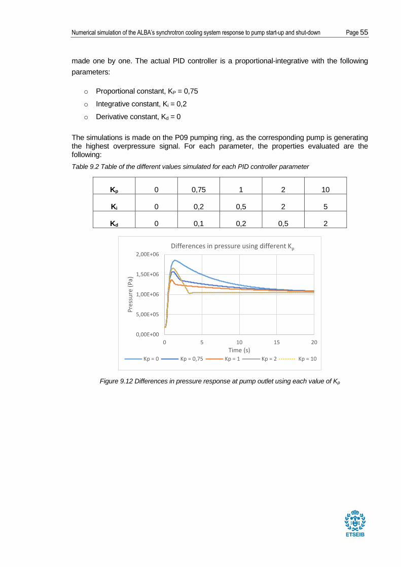
Numerical simulation of the ALBA’s synchrotron cooling system response to pump start-up and shut-down Page 55
made one by one. The actual PID controller is a proportional-integrative with the following
parameters:
o Proportional constant, KP = 0,75
o Integrative constant, Ki = 0,2
o Derivative constant, Kd = 0
The simulations is made on the P09 pumping ring, as the corresponding pump is generating the highest overpressure signal. For each parameter, the properties evaluated are the following:
Table 9.2 Table of the different values simulated for each PID controller parameter
Kp 0 0,75 1 2 10
Ki 0 0,2 0,5 2 5
Kd 0 0,1 0,2 0,5 2
Figure 9.12 Differences in pressure response at pump outlet using each value of Kp
0,00E+00
5,00E+05
1,00E+06
1,50E+06
2,00E+06
0 5 10 15 20
Pre
ssu
re (
Pa)
Time (s)
Differences in pressure using different Kp
Kp = 0 Kp = 0,75 Kp = 1 Kp = 2 Kp = 10

Page 56 Report
Figure 9.13 Differences in pressure response at pump outlet using each value of Ki
Figure 9.14 Differences in pressure response at pump outlet using each value of Kd
According to the results obtained from testing different parameters, it is verified that PID
controller can be improved in order to achieve better response in peak pressure. For the
proportional constant, setting Kp = 1, the simulation produces a pressure peak of 32% the
pressure set point while the pressure peak with the original Kp arrives to the 54%. The
simulations testing different values of Ki and Kd did not show any significantly difference in
pressure peak but they do in the pressures slope.
As a consequence of the result obtained, it is verified that there is room for improvement in the
field of digital control technology by adjusting the PID controlled in our system.
0,00E+00
5,00E+05
1,00E+06
1,50E+06
2,00E+06
0 5 10 15 20
Pre
ssu
re (
Pa)
Time (s)
Differences in pressure using different Ki
Ki = 0 Ki = 0,2 Ki = 0,5 Ki = 2 Ki = 5
0,00E+00
5,00E+05
1,00E+06
1,50E+06
2,00E+06
0 5 10 15 20
Pre
ssu
re (
Pa)
Time (s)
Differences in pressure using different Kd
Kd = 0 Kd = 0,1 Kd = 0,2 Kd = 0,5 Kd = 2

Numerical simulation of the ALBA’s synchrotron cooling system response to pump start-up and shut-down Page 57
9.2. Unexpected pump shut-down
The shut-down of the cooling system should take place when there is not heat generation,
which means that the electromagnets are not activated. However, the system might also
experience pumping failures when the synchrotron is in normal working state.
According to ALBA’s synchrotron needing, the scope of this simulation is the following:
Investigation of unexpected pumps’ stops. It may happen when synchrotron is in
operating state or not. For this reason, two different simulations are made; with no heat
transfer and with heat transfer. The pumps’ stop analyzed are the followings:
- Shut-down of P07 pump
- Shut-down of P09 pump
- Shut-down of P08 pumps (stop of one pump)
(both two pumps simultaneously)
- Shut-down of P10 pumps (stop of one pump)
(both two pumps simultaneously)
- Shut-down of P11 pump
Simulation of the simultaneous pumps’ stop. This simulation aims at analyzing the stop
of the cooling system when all pumps are stopped simultaneously. This simulation is
made without thermic effect as it is supposed that the synchrotron is not operating
when this action is taken.
9.2.1. System’s response with no heat transfer
In the adjusted model, the scripts that regulate the opening of the three ways valves, in function
of the temperature, have been removed and the valves opening has been set at 50%. The
power exchanged in heat exchangers has been set at zero and these components only act as
a pressure loss.
i. Shut-down of P08A pump (stop of one pump)
Pumps P08 are two pumps (A and C) mounted in parallel. As their components are identical,
the simulations show same results for both P08 pumps when they act simultaneously.
However, this simulation simulates the failure and shut-down of the P08A pump. As a
consequence, a transient state starts because the pressures are not in equilibrium anymore.
In P08 pumping ring, the pressure decreases from the pressure set point immediately.
As a response, P08C PID controller, sends the signal to its pump to increase the rotational
speed and gain pressure until the pressure set point is reached. The flow rate that was divided

Page 58 Report
into two pumps, now is suctioned only by P08C pump. As P08C is powerful enough, the
pressure set point is reached and its flow rate is doubled. Thus, the transient events ends when
the pressure set point is reached again in the pumping lines and the system returns to its
nominal operating state. The time need to reestablish the stationary state is 50 seconds.
Figure 9.15 Transient event experienced in P08C pump outlet when P08A pump is stopped
The effect of the transient event in P08 pumping ring is showed in the following pictures:
Figure 9.16 Flow rate and valve opening evolution in P08 pumping line
250
260
270
280
290
300
310
320
8,00E+05
8,50E+05
9,00E+05
9,50E+05
1,00E+06
1,05E+06
1,10E+06
1,15E+06
0 10 20 30 40 50
Ro
tati
on
al s
pee
d (
rad
/s)
Pre
ssu
re (
Pa)
Time (s)
Evolution of P08C pump's pressure and rotational speed
Pressure at pump P08C outlet Rotational speed
0
0,2
0,4
0,6
0,8
1
-0,02
0
0,02
0,04
0,06
0,08
0 0,5 1 1,5 2
Val
ve li
ft
Flo
w r
ate
(m3/s
)
Time (s)
Effect of the transient state and the closure of valve in P08 pumps flow rate
P08A pump's flow rate P08C pump's flow rate P08A valve lift

Numerical simulation of the ALBA’s synchrotron cooling system response to pump start-up and shut-down Page 59
Figure 9.17 Reaction in P08A pumping line to its pump closure
As it can be inferred from the figures above, the closure of the valve happens around 0,8
seconds after the simulation’s start and it has an impact in the system. In this situation, the
valve does not close fast enough and flow rate moves in reverse direction during 0,3 seconds
until the valve closes.
In Figure 9.16, it is seen that the flow in P08A piping line is suctioned by P08C pump. As a
consequence, the flow changes its direction and moves downstream until the valve closes.
When the P08A valve closes, a disturbance is generated through all the pumping lines. At the
outlet of the valve, the phenomena of water hammer is created. The phenomena has a small
amplitude and disappears in less than 0,5 second.
At P08A pump, the drop of pressure reaches the vapour pressure and cavitation occurs at 0,8
seconds, even though the pressure recovers immediately. Furthermore, the closure of the
valve produces more consequences. Firstly, it generates a negative pressure wave that travels
and generate an immediate pressure drop through all the piping system. See in Figure 9.17
the drop in pressure propagated in the other pumping lines.
00,10,20,30,40,50,60,70,80,91
0,00E+00
2,00E+05
4,00E+05
6,00E+05
8,00E+05
1,00E+06
1,20E+06
0 0,5 1 1,5 2
Val
ve li
ft
Pre
ssu
re (
Pa)
Time (s)
Evolution of the transient state in P08A pumping line
Pressure at pump outlet Pressure at pump inlet
Pressure at valve outlet P08A valve lift

Page 60 Report
Figure 9.18 Pressure drop detected in the other pumping lines
Secondly, when P08A is stopped, the system pressure start to fluctuate as it is not stable.
When the valve closes, the amplitude of the pressure drop is higher than the pressure
fluctuation and, as a result, the amplitude of the pressure fluctuation increases. Hence, the
system needs more time to reach the stationary state, around 50 seconds to reach the
pressure set point again. The pressure fluctuations disappear after 20 seconds.
The fluctuation of pressure leads to the PID controllers to send sinusoidal signals to the pumps,
which are converted into a sinusoidal variation in the rotational speed of each pump. These
consequences can be noticed in the figures below.
Figure 9.19 Amplitude increases after the valve closure Figure 9.20 Relation between pressure and rotational speed
With regard to the other pumping lines, the highest effects of the P08A pump’s stop can be
seen in the common return line because it is connected directly, as flow travels from the P08
pumping ring to the return line.
7,50E+05
8,00E+05
8,50E+05
9,00E+05
9,50E+05
1,00E+06
1,05E+06
1,10E+06
0 0,5 1 1,5 2
Pre
ssu
re (
Pa)
Time (s)
Pressure drop propagated through the system
P07 P09 P10
0
0,2
0,4
0,6
0,8
1
1,03E+06
1,04E+06
1,05E+06
1,06E+06
1,07E+06
1,08E+06
1,09E+06
1,10E+06
1,11E+06
0 1 2 3
Tim
e (s
)
Pre
ssu
re (
Pa)
Time (s)
Pressure amplitude increases after valve's closure
Pressure at pump P10 outlet P08A valve lift
292
293
294
295
296
297
298
299
1,03E+06
1,04E+06
1,05E+06
1,06E+06
1,07E+06
1,08E+06
1,09E+06
1,10E+06
1,11E+06
0 1 2 3
Tim
e (s
)
Pre
ssu
re (
Pa)
Time (s)
Rotational speed changes in relation to the pressure variation
Pressure at pump P10 outlet Rotational speed

Numerical simulation of the ALBA’s synchrotron cooling system response to pump start-up and shut-down Page 61
See in the figures below, the effect of the transient state in the common return line (P11). As
the pressure set point for P11 pump is 3,5·105 Pa, when the pressure value surpasses the set
point level, the PID controller sends the signal to reduce the rotational speed and, on the other
hand, when the pressure lowers the set point value, the pump rotational speed gets increased
until its maximum in case the pressure has not arrived yet to the set point value. The maximum
pressure oscillations happens after the valve closure and have an amplitude of 0,3·105 Pa.
Figure 9.21 P11 pump behavior during P08A stop
Figure 9.22 Evolution of P11 pumping line flow rate
0 2 4 6 8 10
154,5
155
155,5
156
156,5
157
157,5
0,00E+00
5,00E+04
1,00E+05
1,50E+05
2,00E+05
2,50E+05
3,00E+05
3,50E+05
4,00E+05
4,50E+05
Ro
tati
on
al s
pee
d (
rad
/s)
Pre
ssu
re (
Pa)
Time (s)
Pressure and rotational speed in the common line return
Pressure at pump outlet Rotational speed
0,1682
0,1684
0,1686
0,1688
0,169
0,1692
0,1694
0,1696
0,1698
0 2 4 6 8 10
Pre
ssu
re (
Pa)
Time (s)
Common return line flow rate during the first 10 seconds
Flow rate pump

Page 62 Report
With regard to the flow distribution, it will be back to the operating state once the system
reaches the pressure equilibrium. Then, the flow distribution will be exactly the same as the
normal operating system because P08C pump can counteract the pressure loss and maintain
the pressure at the set point level.
There is a decrease in the flow suctioned to the pumping lines because the pump’s force of
suction is reduced as P08A pump is stopped. Then, the flow that moves from the pumping
lines to the P11 pump is less than in operational state and, as a results, P11 pump suctions
more flow from the accumulator, the difference of flow that is not obtaining from the pumping
lines.
The transient evolution of the flow rate is seen in the following figure:
Figure 9.23 Evolution of the flow rate distribution in the system as a consequence of P08A pump stop
ii. Shut-down of P08 pumps simulation (both two pumps simultaneously)
In this simulation, it is modelled and simulated the stop of the two P08 pumps. The main
interest about this simulation is to see how pressure changes while a whole pumping station
turns as inoperative. The fluidic dynamic simulation is also a case of study.
The results of the system’s response has showed that stopping a whole ring results in a
transient state where pressure, rotational speed and flow oscillate until a new state of pressure
equilibrium. The duration of this transient event is about 25 seconds, when the valve closes
entirely. However, in this case, the closure does not produce any effect in the system as the
pressure slope is nearly flat. Before its closure, the valve oscillates because flow is constantly
being reduced as the P08 pumps do not suction anymore.
0,07
0,075
0,08
0,085
0,09
0,095
0 5 10 15 20
Flo
w r
ate
(m3 /
s)
Time (s)
Evolution of flow rate in the piping system
Flow through the connection of common return line-pumping lines
Flow from the accumulators to the common line
Flow from the accumulator to the pumping lines

Numerical simulation of the ALBA’s synchrotron cooling system response to pump start-up and shut-down Page 63
Figure 9.24 Behavior of P08 pumps when they are forced to stop
The effects seen in other pumping lines are higher than in previous simulation. As the most
affected pump line is the P11 pump line (common return line), only these results are exposed
in this section.
Figures 9.25 Behavior of P11 pumps when P08 pumps are stopped
See Annex section H to see the pressure, rotational speed and flow rate variation in each
pumping ring when P08 pumps closes.
With regards to the flow distribution. Due to the stop of P08 pumps, the pumping lines cannot
suction as much flow as before. As a consequence, the flow rate that moves from the
accumulator and the connection mixing valves to the pumping lines decreases and the
0 10 20 30
0
0,2
0,4
0,6
0,8
1
0,00E+00
2,00E+05
4,00E+05
6,00E+05
8,00E+05
1,00E+06
1,20E+06
Val
ve li
ft
Pre
ssu
re (
Pa)
Time (s)
Evolution of P08 pumps outlet pressure and valve's closure
Pressure at pump outlet Valve lift
0
50
100
150
200
250
300
0 10 20 30 40
Ro
tati
on
al s
pee
d (
rad
/s)
Time (s)
Evolution of P08 pumps rotational speed
Rotational speed
154,5
155
155,5
156
156,5
157
157,5
0,00E+00
1,00E+05
2,00E+05
3,00E+05
4,00E+05
5,00E+05
0 10 20
Ro
tati
on
al s
pee
d (
rad
/s)
Pre
ssu
re (
Pa)
Time (s)
Evolution of the common line properties
P11 Pressure at pump outlet
P11 Pressure at pump inlet
P11 Rotational speed
0,1682
0,1684
0,1686
0,1688
0,169
0,1692
0,1694
0,1696
0,1698
0 5 10 15 20
Flo
w r
ate
(m3 /
s)
Time (s)
Flow rate evolution in common return line
Flow rate

Page 64 Report
accumulator moves more water to the common return line (P11 pump).
Figure 9.26 Evolution of the flow rate distribution in the system as a consequence of P08 pumps stop
iii. Stop of P10A pump simulation (stop of one pump)
P10 pumps are two pumps (A and C) mounted in parallel. This simulation simulates the failure
and stop of the P10A pump. As a consequence, a transient state starts because the pressures
are not in equilibrium. This simulation will lead to a different response of the system than the
obtained stopping P08A pump as the pumps are different.
Figure 9.27 Behaviour of P10C pump when P10A pump is forced to stop
In this case, when the P10A pump stops, P10C pump increases its rotational speed in order
to maintain the pressure set point. However, P10 pumps have less power than P08 and the
0
0,02
0,04
0,06
0,08
0,1
0,12
0 5 10 15 20
Flo
w r
ate
(m3/s
)
Time (s)
Evolution of flow rate in the piping system
Flow through the connection of common return line-pumping lines
Flow from the accumulators to the common line
Flow from the accumulator to the pumping lines
290
295
300
305
310
315
320
0,00E+00
2,00E+05
4,00E+05
6,00E+05
8,00E+05
1,00E+06
1,20E+06
0 2 4 6 8 10
Ro
tati
on
al s
pee
d (
rad
/s)
Pre
ssu
re (
Pa)
Time (s)
Evolution of P10C pump's pressure and rotational speed
Pressure at P10C pump outlet Rotational speed

Numerical simulation of the ALBA’s synchrotron cooling system response to pump start-up and shut-down Page 65
pump reaches its maximum rotational speed and can’t counteract the pressure’s decreases.
As a result, pressure and flow travelling by P10 pumping ring are reduced. The closure of the
P10A valve generates a brief water hammer at the valve outlet and increases the amplitude of
the pressure oscillations.
Figure 9.28 Effect of the P10 pump stop in P10 line Figure 9.29 Behavior of the P10A pump when it is stopped
The following figure show the distribution of flow rate until the new stationary state is
reached.
Figure 9.30 Changes in flow system due to the shut-down of P10A pump
0
0,2
0,4
0,6
0,8
1
-0,01
0,01
0,03
0,05
0,07
0 1 2V
alve
lift
Flo
w r
ate
(m3 /
s)
Time (s)
Effect of the transient state and the closure of valve in P10 pumps flow
rate
Flow rate pump P10C Flow rate pump Valve lift
0
0,2
0,4
0,6
0,8
1
0,00E+00
2,00E+05
4,00E+05
6,00E+05
8,00E+05
1,00E+06
1,20E+06
0 1 2
Val
ve li
ft
Pre
ssu
re (
Pa)
Time
Pressure evolution of the transient state in P10A
Pressure at pump outlet Pressure at pump inlet
Pressure at valve outlet Valve lift
0,06
0,08
0,1
0,12
0,14
0,16
0,18
0 1 2 3 4 5 6 7 8 9 10
Flo
w r
ate
(m3
/s)
Time (s)
Evolution of system's flow rate
Flow to P11 pump line Flow through the connection of common return line-pumping lines
Flow from the accumulators to the common line Flow from the accumulator to the pumping lines
Flow from the pumping lines

Page 66 Report
iv. Stop of P11 pump
In this simulation, it is modelled and simulated the shut-down of P11 pump.
This line is working at the lowest pressure set point of the pumping lines, 3,5·105 Pa. When
P11 pump is stopped, the valves also closes slowly. As a consequence, the pressure
perturbations caused in the system are less important than in P08 or P10 pumps shut-down.
Thus, in this simulation it is a case of interest the flow distribution of the system as this pump
brings the water to the heat exchangers for cooling the water, which is important when the
cooling system is cooling down the ALBA’s electromagnets.
With regards to the flow distribution system response, once the P11 pump is stopped, flow to
P11 pump line decreases until zero and the pumping are the only ones suctioning the water.
As P11 pump does not suction flow anymore, flow from the accumulator to the common return
line reverses its direction and travels from the common line to the accumulator. The following
figure, shows the evolution of the flow distribution in the system once the P11 pump is stopped.
Figure 9.31 Evolution of flow inside the system
v. Stop of the rest of pumps
The following stops can be find in Annex section H:
o Stop of P10 pumps simulation (both two pumps simultaneously): simulation is very
similar to the P08 pumps’ stop. The fluctuation of the pressure and rotational values
are less significant in the other pumping lines as P10 pumps suction less flow than P08
pumps.
-0,1
-0,05
0
0,05
0,1
0,15
0,2
0 5 10 15 20Flo
w r
ate
(m3/s
)
Time (s)
Flow distribution evolution in the piping system
Flow to P11 pump line
Flow through the connection of common return line-pumping lines
Flow from the accumulators to the common lines
Flow from the accumulator to the pumping lines

Numerical simulation of the ALBA’s synchrotron cooling system response to pump start-up and shut-down Page 67
o Stop of P07 and P09 pumps: the simulation is similar to stopping the pumps in other
pumping stations. As both pumps move less flow than P08 and P10 pumping lines, the
effect in the other rings are less significant.
9.2.2. System’s response with heat transfer
The study of these simulations aims at finding problems if any of the pumps fail and, as a
consequence, stop when the synchrotron is in operating state, which means that heat at the
ring is continuously generated. The objective of the study is to determine if there are any
pressure and temperature problems as a result of the failure and the effects in the whole
system.
From the System’s response with no heat transfer simulations, it was verified that the highest
pressure oscillations were taking place due to P08A or P10A pump shut-down. With regards
to the other simulations, the pressure effects were not as significant as the mentioned
previously and the behavior was similar. For this reason, in this section it is only studied the
P10A pump shut-down with heat transfer.
The shut-down of the P11 pump is also a case of study because the previous simulation, with
no heat transfer, has showed that flow gets suctioned from the pumping lines, and,
consequently, it does not reach the heat exchanger. Then, in this simulation, the flow
distribution plays a critical role in the thermic response of the system.
i. Shut-down of P10A pump simulation
From the data obtained it is verified that there is not a significant difference in pressure. See it
in next figure.
Figure 9.32 Evolution during P10A pump shut-down
0
0,2
0,4
0,6
0,8
1
7,00E+04
1,20E+05
1,70E+05
2,20E+05
0 5 10 15 20
Val
ve li
ft
Pre
ssu
re (
Pa)
Time (s)
Evolution of properties during the P10A pump shut-down
With heat transfer: Pressure at pump inlet With no heat transfer Pressure at pump inlet
With heat transfer: Valve Lift With no heat transfer Valve Lift

Page 68 Report
Hence, the analysis is focused on detecting changes in system’s flow rate and temperature.
As for the flow rate distribution, when the pump is stopped (at 5 seconds), the position of the
three way valve changes from 0,75 to 0,765, increasing minimally the flow rate from the
common return.
Figure 9.33 Evolution of the flow rate
Once 10A pump is stopped, less flow travels inside the line. As a consequence, the
temperature at heat exchanger outlet increases. The increase is small, less than 1°C.
Figure 9.34 Temperature evolution in the system
0,02
0,025
0,03
0,035
0,04
0,045
0,05
0,745
0,75
0,755
0,76
0,765
0,77
0 5 10 15 20
Flo
w r
ate
(m3 /
s)
Val
ve li
ft
Time (s)
Evolution of the flow rate distribution in P10 pumpiing line
Three way valve
Flow from the accumulator (cooled water)
Flow from the common return (heat water)
293
294
295
296
297
298
299
0 5 10 15 20
Tem
per
atu
re (
K)
Time (s)
Evolution of the temperatures in the system
Temperature after mixing Temperature of the flow from the accumulator
Temperature of the flow from the common return Temperature at ring inlet
Temperature at ring outlet

Numerical simulation of the ALBA’s synchrotron cooling system response to pump start-up and shut-down Page 69
ii. Shut-down of P11 pump simulation
The previous simulation with no heat transfer was useful to determine the flow distribution.
Based from the flow distribution obtained, the thermal behaviour is the case of study in this
simulation because when the P11 pump is stopped, the flow doesn’t move through the
common line return and consequently, the flow is not cooled and it gets hotter as it moves
through the consumption rings.
The following images show the system’s local response (with a short period of time) after the
pump’s shut-down.
Figure 9.35 Evolution of the flow rate during the first 25 seconds of the transient state
Figure 9.36 Evolution of the valve closure as a consequence of the pump shut-down
-0,1
-0,05
0
0,05
0,1
0,15
0,2
0 5 10 15 20 25 30Flo
w r
ate
(m3 /
s)
Time (s)
Evolution of flow rate
Flow to P11 pump line
Flow through the connection of common return line-pumping lines
Flow from the accumulator to the common lines
Flow from the accumulator to the pumping lines
Flow at the pumping lines
0,68
0,7
0,72
0,74
0,76
0,78
0 5 10 15 20 25 30
Val
ve o
pen
ing
Time (s)
Evolution of the valve closure slope
P07 Three ways valve opening P08 Three ways valve opening
P09 Three ways valve opening P10 Three ways valve opening

Page 70 Report
Figure 9.37 Evolution of the temperature in two different points in the pumping lines
In Figure 9.35, it can be validated the assumption that the flow rate suctioned in the P11
pumping line tends to zero when the P11 pump is stopped. In Figure 9.36 and Figure 9.37 it
can be seen that the change in the valve’s lift produce an immediate change in the temperature
at the three ways valves outlets. However, it can also be seen that the flow needs some more
time to arrive to the swing-check valve. In consequence, the time for the flow to move through
all the system is longer and requires more tie as exposed in the next figures.
Long simulation
Figure 9.38 Evolution of opening from hot and cold water in each pumping line
296
296,2
296,4
296,6
296,8
0 5 10 15 20 25 30
Tem
per
atu
re (
K)
Time (s)
Evolution of temperature
P07 Temperature at three way valve outlet P08 Temperature at three way valve outlet
P09 Temperature at three way valve outlet P10 Temperature at three way valve outlet
P07 Temperature at swing check valve outlet P08 Temperature at swing check valve outlet
P09 Temperature at swing check valve outlet P10 Temperature at swing check valve outlet
0
0,1
0,2
0,3
0,4
0,5
0,6
0,7
0,8
0,9
0 100 200 300 400 500 600 700 800
Val
ve li
ft
Time (s)
Three ways valves opening evolution in each pumping ring
P07 P08 P09 P10
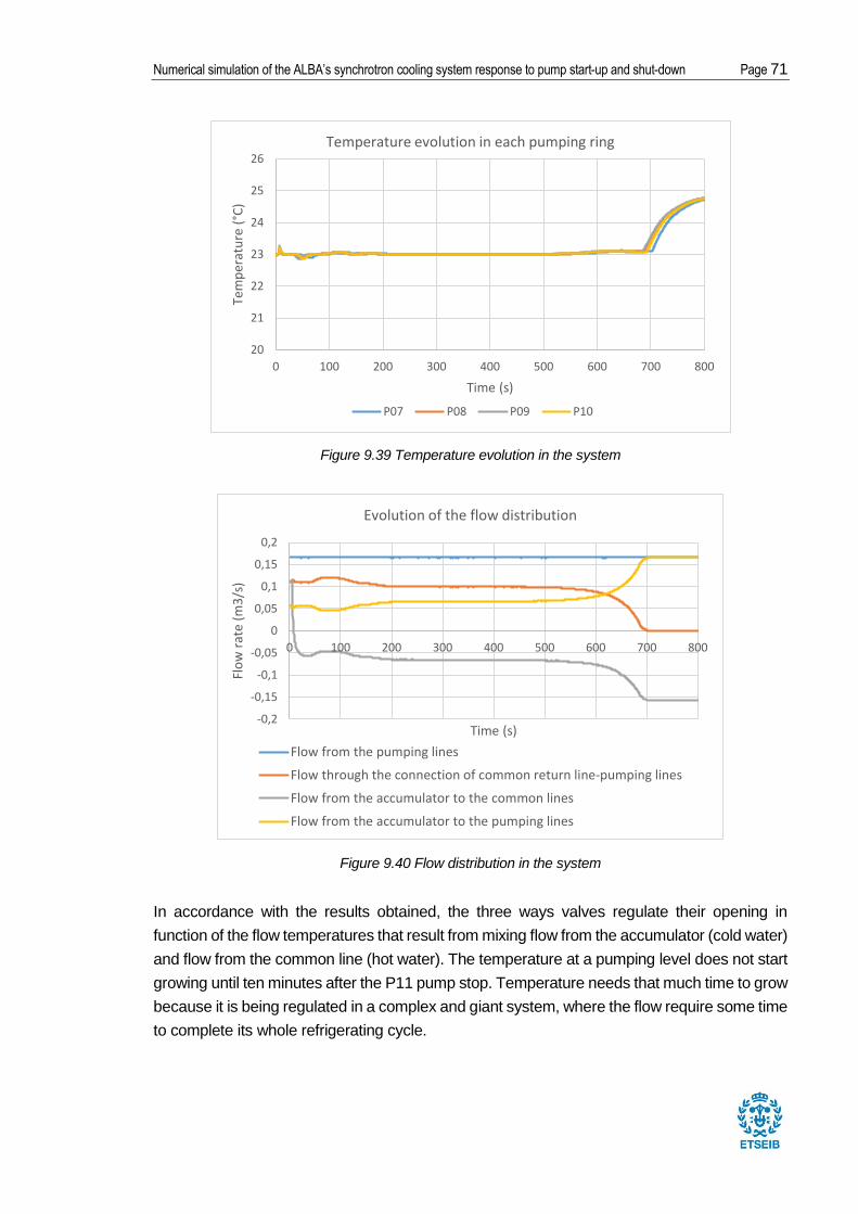
Numerical simulation of the ALBA’s synchrotron cooling system response to pump start-up and shut-down Page 71
Figure 9.39 Temperature evolution in the system
Figure 9.40 Flow distribution in the system
In accordance with the results obtained, the three ways valves regulate their opening in
function of the flow temperatures that result from mixing flow from the accumulator (cold water)
and flow from the common line (hot water). The temperature at a pumping level does not start
growing until ten minutes after the P11 pump stop. Temperature needs that much time to grow
because it is being regulated in a complex and giant system, where the flow require some time
to complete its whole refrigerating cycle.
20
21
22
23
24
25
26
0 100 200 300 400 500 600 700 800
Tem
per
atu
re (
°C)
Time (s)
Temperature evolution in each pumping ring
P07 P08 P09 P10
-0,2
-0,15
-0,1
-0,05
0
0,05
0,1
0,15
0,2
0 100 200 300 400 500 600 700 800
Flo
w r
ate
(m3
/s)
Time (s)
Evolution of the flow distribution
Flow from the pumping lines
Flow through the connection of common return line-pumping lines
Flow from the accumulator to the common lines
Flow from the accumulator to the pumping lines

Page 72 Report
9.2.3. System’s response to a simultaneous pumping stoppage
The objective of this simulation is to determine if whether the technicians could or should stop
all the pumps at the same time or not in a critic case. The actual shut-down steps in the cooling
system are the following:
1. Stop of P07 pump
2. Stop of P08 pumps
3. Stop of P09 pump
4. Stop of P10 pumps
5. Stop of P11 pump
Note that all steps are sequential, when one pump stops and the system stabilizes, next pump
is stopped.
The following figures are a collection of the data obtained from the simulation, where some
relevant information can be inferred.
Figure 9.41 Pressure evolution at the pump outlet
1,20E+05
3,20E+05
5,20E+05
7,20E+05
9,20E+05
1,12E+06
0 5 10 15 20
Pre
ssu
re (
Pa)
Time (s)
Evolution of pressure at pump outlet
P07 P08 P09 P10 P11

Numerical simulation of the ALBA’s synchrotron cooling system response to pump start-up and shut-down Page 73
Figure 9.42 Pressure oscillations at pump inlet
Figure 9.43 Evolution of the valves closures
From the results obtained it can be inferred that the stoppage of all pumps at once is producing
more amplitude pressure oscillations than closing sequentially and all the valve closure is
delayed. It is a consequence of stopping all the power of suction. In other words, when only
one pump line is being shut-down, the power of suction from the other pumps, make the
transient state a shorter period in time compared to stopping all the pumps at the same time.
Moreover, as valve closes slowly, the system does not experience water hammer either
cavitation phenomena. The closure valves slopes also show relevant information about the
closure of the valves. The information is the following:
1,00E+05
1,40E+05
1,80E+05
2,20E+05
2,60E+05
3,00E+05
0 5 10 15 20
Pre
ssu
re (
Pa)
Time (s)
Evolution of pressure at pump inlet
P07 P08 P09 P10 P11
0
0,1
0,2
0,3
0,4
0,5
0,6
0,7
0,8
0,9
1
0 5 10 15 20 25 30
Val
ve li
ft
Time (s)
Evolution of the valve closure
P07 P08 P09 P10 P11

Page 74 Report
The higher quantity of flow in the line, the latest the valve starts to close. By this fact,
in ascending order (from earlier to later) the closure slopes are: P09 < P07 < P10 <
P08 < P11.
The higher the pressure set point is, the latest the valve finishes its closure. The order
of closure from earlier to later is: P11 < P07 < P09 < P10 < P11. Even though P09
pressure set point is slightly higher than P10 pressure set point, as P09 pumping line
brings eight times less flow than P10 pumping line, P09 valve closes before.
9.3. System’s response to presence of air
In Flowmaster simulations, it is assumed that the pipes only contain liquid inside and no air
can be found, only counted in case of cavitation. However, it is known by the R&D department
from ALBA’s synchrotron that there are air formations near the rings, and they have had
problems specifically in the Service ring area.
An accumulator of air vessel can simulate the effect on the pressure response of the system
of air in the pipes. Air in pipes minimizes the pressure oscillations as it absorbs them. For this
reason, an air vessel accumulator has been placed near the rings area during the shut-down
of the pumps.
For this simulation, the test will be focused in the shut-down of P08 pumps (both pumps
simultaneously) as the highest pressure perturbations in the system have been noticed in this
case. See in the next image, the place where the accumulator is set.
Figures 9.44 Place where the accumulator is set

Numerical simulation of the ALBA’s synchrotron cooling system response to pump start-up and shut-down Page 75
The simulation is evaluated at the accumulator outlet in order to verify the accumulator
effectivity.
The simulation evaluates the effect of different accumulator’s height, which is traduced as the
quantity of air that the pipes holds inside. The height will comprise the following values:
• No accumulator
• 0,01 ; 0,5 ; 1 ; 2
9.3.1. System’s responses to air level inside the accumulator
In the Figure 9.45 it can be seen the different pressure responses according different quantities
of air. Hence, it is validated that air minimizes the pressure waves.
It can be observed that with a reduced quantity of air, the signal still shows big pressure
amplitudes. When the air volume is increased, the pressure amplitude decreases and also the
frequency of the waves. With a high quantity of air, the pressure waves are absorbed.
Figure 9.45 Differences by setting different quantities of air
It may be seem that air is a solution in order to minimize pressure oscillation but, in fact, air in
pipes can generate a range of problems, such as:
o Air reduces the effective diameter and, as a consequence, it results as a reduction in
the pipe’s capacity.
o The presence of air may modify the turbulence structure of the fluid and also the wall
shear.
o Air can facilitate the corrosion as it provides with more oxygen.
1,00E+05
1,20E+05
1,40E+05
1,60E+05
1,80E+05
2,00E+05
2,20E+05
2,40E+05
0 5 10 15 20
Pre
ssu
re (
Pa)
Time (s)
Evolution of the pressure at the accumulator outlet
A = 0,01 A = 0,5 A = 1 A = 2 No accumulator

Page 76 Report
9.4. Summary of results
With regards to the start-up of the system, firstly, it has been necessary to introduce new scripts
in order to successfully simulate the transient conditions imitating the real start-up in ALBA’s
synchrotron. Thereupon, it has been proceeded to the evaluation of the simulation response.
Firstly, it is detected an overpressure in the start of each pump. The overpressure generated
due to the pump’s acceleration and inertia may reduce the life-time of the piping components.
Although it is out of this project’s scope, it has been proposed to study and modify the
characteristic parameters of the PID controllers (Kp, Ki, Kd) in order to find out the optimum
values for the system.
With regards to the design and PID implementation, the adjusted model, designed for this
project, can be used in order to find out the optimum values and verify the overpressure
generated at the pumps outlet. The tests made in this project has showed up the following
improvement. The overpressure’s for P09 start-up can be reduced from 54% to 32% if the
proportional constant is set at 1, instead of 0,75.
It is also observed that the pump’s start-up generates pressure variations in the other pumping
lines, yet, the variations are residual and appear not to be very dangerous. The start-up has a
duration of 100 seconds.
With regards to the stoppage of the system, the following studies have been focused in
unexpected pumps shut-down. The first part has comprised the analysis of the model with no
heat transfer and the second part has included the thermal regulation. In general terms, the
pressure distribution has been observed to be the same in both cases.
From the simulations with no heat transfer, the behavior of the system has showed some
patterns:
1. The pressure oscillations produced by a pump shut-down are more significant if the
stopped pump was in a line where more flow moved inside. By this fact, the shut-down
of P08 and P10 pumps are the ones that produce higher perturbations in the other
pumping lines. However, the perturbations are not too high and they stop in a short
range of time.
2. The unexpected shut-down of one of the two pumps mounted in parallel that operate
in P08 and P10 pumping lines generates during a short period of time water hammer
effects. The reason is that one pump is stopped while the other pump in parallel tries
to compensate the flow reduction, and as a result, the flow quickly changes its direction,
provoking a very fast closure of the non-return valve’s lift. Thus, the phenomena of
Numerical simulation of the ALBA’s synchrotron cooling system response to pump start-up and shut-down Page 77
water hammer is generated at the valve outlet and it enlarges the pressure oscillations
of the system, probably generating cavitation as the pressure reaches the vapor
pressure during an instant of time.
3. The shut-down of all the pumps in one line does not produce any dangerous
phenomena for the piping system. The process of shut-down is slow and the valve
closure variates its opening during the transient event. Finally, when the valve closes
totally, the pressure and flow rate in the line has been reduced significantly and, as a
consequence, pressure variations are short in time and in amplitude.
4. In all the simulations, the most affected pumping line is the common return line and it
is because we are simulating a closed piping system where the flow from the pumping
lines converge in the common return line.
5. When the P11 pump is stopped, the flow distribution changes completely. A new flow
distribution is achieved comprising only the consumption side. The residual flow now
moves to the accumulator, which will be suctioned by the pumping lines. As a result,
the flow does move through the coolers.
6. The system response to a simultaneous stoppage of all pumps shown that there are
not potential problems in the pumping lines. However, oscillations in pressure may
become more significant in this case.
From the simulations with heat transfer, the following simulations were proposed:
Shut-down of P10A pump: aimed at finding out if with thermal changes, the water
hammer was also appearing in the system’s response.
Shut-down of P11 pump: aimed at analyzing the system’s thermal response as the
flow does not moves through the coolers.
From the results obtained by the previous two tests, it is noticed that, in first place, the
temperature of the pumping line variates around ±0,5°C when the pumps stop and the valves
close. For this reason, the pressure response seen in the simulation with and with no heat
transfer is very similar.
The first simulation, shut-down of P10A pump, has showed that the system is robust against
this level of flow variations. The reduction of flow in the P10 pumping line has the
consequences to increase 1°C more than the flow temperature at the heater exchange outlet.
It is not even noticed in the other lines in the system as it is compensated by the change in the
three ways valve opening ratio.

Page 78 Report
The second simulation, shut-down of P11 pump, has showed that the system’s temperature
needs around ten minutes to increase and to notice that the P11 pump was stopped. At eleven
minutes from the stop of P11 pump, the three ways valves closes totally and only the flow from
the accumulator can move through the pumping lines. It is a consequence of the temperature
increase in the system and it tries to cold down letting more of the flow from the accumulator.
However, the accumulator’s flow is not cooled down and the temperature continues rising.
Finally, the last simulation has intended to do a more realistic simulation. In Flowmaster model,
the air generation in the pipes cannot be modelled unless the air is created by cavitation. In
this simulation, the set of an air vessel accumulator has pretended to simulate an air’s bag.
The results have shown that the pressure oscillations are more absorbed if there is more air in
the system. However, it must be kept in mind that air is a problem for the piping system and
not a solution, although it reduces the pressure oscillations.

Numerical simulation of the ALBA’s synchrotron cooling system response to pump start-up and shut-down Page 79
10. Project scheduling
According to the project’s necessities, an adequate action plan was designed in order to meet deadlines and objectives of this study. Its
proposal is just indicative and it is a good reference to know how the project’s progress is. As it is known, technical projects may experiences
difficulties and contingencies and it does not mean that every part must be finished in the predetermined time but the planning helps to
achieve your plans in time, with good results and presentation. Project’s planning has been designed with a Gantt chart.
10.1. Gantt diagram

Page 80 Report
11. Environmental impact
The simulations executed and presented in the present document may be beneficial in order
to detect instabilities and piping problems related to pressure changes in transient events.
Hence, this identification allows to identify possible problems in time, which it leads to
economic expense reduction in possible problems that may appear in the system.
Moreover, the operations that are needed in order to repair a component in the piping system
must be done without any fluid in the pipes. It means that the system must be drained. The
deionized water may be contaminated due to losses and friction in the pipes. Therefore, the
refill must be done with new pure deionized water and the contaminated water must be
properly recycled. Avoid emptying and refilling the system, it leads to energy and fluid saving.
Also, the recycling cost of water is reduced.
Avoiding problems is not only good in environmental field but also means minimizing the time
needed in repairing and time is worthy.
Moreover, the determination of the system response using numeric simulations instead of
physical experimentation, it is traduced in energy saving. As the physical system is not tested
under extreme conditions, it is avoided to wear off the piping components and component life-
time is not reduced.

Numerical simulation of the ALBA’s synchrotron cooling system response to pump start-up and shut-down Page 81
12. Project budget
The project budget has been designed according the structure of the budget of material
execution, whose abbreviation is PEM in Spanish.
For this design, expenses related to employee and material to perform this project has been
taken into account.
The project has been led by a junior engineer dedicated exclusively in this project for a total of
300 hours. The supervision has been taken by a senior engineer with a dedication of 30 hours
along the project. See in next table the project budgets for material and employee.
Table 12.1 Expenses of the project
Cost of the employee
Resources requirements Units (h) Unit cost
(€/h) Cost (€)
1 Junior engineer 300 15 4500
Junior engineer social security expenses (7%)
315
1 Senior engineer 30 30 900
Senior engineer social security expenses (33%) 297
TOTAL
6012
Cost of material
Material needing Initial
cost (€)
Amortization period (years)
Annual amortization
(€/year) Time
(years)
Accumulated amortization
(€)
1 Laptop 900 5 180 0,5 90
Flowmaster license 1000 1 1000 0,5 500
Microsoft Office license
100 5 20 0,5 10
Office expenses, rent and maintenance
1000 1 1 5 500
TOTAL
1100

Page 82 Report
According to the Spanish law, the article 131 of the “Reglamento General de la Ley de
Contratos de las Administraciones Públicas”[9] approved by the Royal Legislative Decree
1098/2001, at 12th October, stablish that the base budget in construction contract will be
obtained incrementing by a 13% the budget of material execution and the 6% as a concept
of benefit to the contractor. The value-added tax will be applied to total of the budget of material
execution and general expenses of the structure.
According to the actual law, FOM/1824/2013 30th September 2013, it is determined the
Contracted Operation Budget indicated in the Table 12.2.
Table 12.2 Contracted Operation Buget
FINAL BUDGET OF THE PROJECT Expenses Cost (€)
Employee cost
6012
Material needing
1100
TOTAL
7112
General expenses (13%)
924,56
Contractor benefit (6%)
426,72
PEM before IVA tax
8463,28
IVA (21%)
1777,29
Contracted operation budget
10240,57
The final budget of the project is TEN THOUSAND AND TWO HUNDRED FORTY EUROS
WITH FIFTY SEVEN CENTS (10.240,57 €), taxes (IVA) includes.

Numerical simulation of the ALBA’s synchrotron cooling system response to pump start-up and shut-down Page 83
Conclusions
It has been confirmed that Flowmaster software meets with the specifications necessary to
successfully model and simulate the different transient situations raised in this project. The
preliminary tests realized with simpler models have verified its utility.
The previous model available of the cooling system has been modified and adjusted in order
to successfully simulate compressible flow effects during fast transient events. With the
readjusted model, the transient simulations have provided reliable results that have led to solid
conclusions.
Regarding to the pumping system start-up, it has been discovered that all the rings are
experiencing significant pressure rises when their corresponding pumps are activated with
maximum values in Booster Ring (P09). The duration of the transient is of about 100 sec.
Based on a series of tests, it has been found that the proper modifications of the PID
parameters can lead to a reduction of these overpressures.
Regarding the pump shut-downs, the change of conditions in one pumping station has
significant effects in the rest of rings and the common return pipe. The highest pressure
perturbations are produced in the rest of the pumping lines when pumps P08 and P10 are
stopped. On the other hand, P07 and P09 stops generate much lower effects on the rest of
the system. This is due to the higher flow rate that is being pumped by P08 and P10 pumping
stations. It is also noticed that the common return line experiences pressure oscillations in all
the cases due to the closed loop system configuration.
The unexpected shut-down of only one of the two pumps at P08 or P10 pumping stations may
bring the system to experience slight water hammer, possible cavitation and higher amplitude
in the pressure oscillations due to the fast closure of the non-return valves. In the P08 ring,
only one pump is capable of compensating the lack of flow rate due to the other pump stop.
However, in the P10 ring when only one pump operates the nominal flow rate cannot be
achieved.
The simultaneous shut-down of all pumps has shown to generate higher pressure oscillations
along the entire system but no water hammer is experienced. Therefore, it might be safe to
shut-down all pumps at the same time in case of emergency.
The shut-down of P11 has a strong effect because it changes completely the flow distribution
in the entire system. It is especially important during thermal regulation because the flow stops
moving through the coolers and the water temperature cannot be controlled and rises. The
thermal transient provoked by the P11 stop reaches the rest of the pumping lines with a delay
of around 10 min. At this point the water temperature starts to rise without control because the

Page 84 Report
three way valves cannot cool the common return water. This is because the water temperature
in the accumulator is already higher than the set point. As a consequence, it is critical to know
the P11 condition to protect the cooling system.
In the case that one of the P08 or P10 pumps fails and stops with the thermal regulation system
in operation, the system can still work effectively due to its robustness against small changes
in flow rates. In this cases, the three way valves will auto-adjust in order to keep the mixed
water temperature at the correct set point.
The presence of air in the pipes has been simulated with accumulators located close to the
rings. It has been confirmed that in the case of a significant amount of air the frequency and
amplitude of the pressure fluctuations are lowered.
In general, all the simulations analyzed are reliable and, in order to successfully end with the
project, the predictions should be validated with experimental measurements at the
synchrotron cooling system.
To conclude, pressure, rotational speed and flow rate fluctuations have been predicted with
short duration and relatively low amplitudes for most of the transient conditions. The different
observed behaviors and the system responses, such as the flow distribution in the pipes, may
be used as a reference to find out if there is any problem regarding to the pumping system
during normal operation. Consequently, it is proposed to monitor these data continuously for
an effective and better system protection.

Numerical simulation of the ALBA’s synchrotron cooling system response to pump start-up and shut-down Page 85
Acknowledgement
I would like to appreciate the help that the mentor of this project, Xavier Escaler, has provide
along the conception and realization of the project.
My thankfulness to his accessibility, dedication to clarify all the concepts and willingness to
help, having him as a great Fluid Mechanical professor during my classes of the subject and
a great mentor in this Bachelor’s Thesis.
Page 86 Report
Bibliography
Bibliographic references
[1] DAVID, C. ALBA Synchrotron Light Source, Infrastructure and General Services. Asset
and Maintenance Management Workshop, 2013. AMMW, Geneva, 2013.
[http://indico.cern.ch/event/233494/session/1/contribution/56/material/slides/7.pdf, 5th
May 2016].
[2] GENERALITAT DE CATALUNYA. GOVERN. Sincrotró ALBA. [http://www.gencat.cat/web/multimedia/cat/sincrotro/index_htm.htm, 9th May 2016].
[3] CELLS. HEALTH AND SAFETY. Health and safety at ALBA (CELLS). Cerdanyola del
Vallès, Salut i seguretat laboral.
[4] BOLUFER, P. ALBA. Anales de mecánica y electricidad. Vol.87 (4), 2010, p. 60-63.
[5] ALBA synchrotron. Beamlines. [https://www.cells.es/en/beamlines, 1st June 2016].
[6] UNIVERSITAT POLITÈCNICA DE CATALUNYA. Piping Systems – EsX. Pg 19-25.
BarcelonaTech. Departament de fluids.
[7] QUISPE, M. Review of ALBA cooling system crisis. Cerdanyola del Vallès, 5th June
2016.
[8] MADRIDEJOS, A. Sincrotrón a toda máquina [en línia]. El Periódico, 4th June 2016,
pg. 2.
[9] Agencia Estatal Boletín Oficial del Estado.
[https://www.boe.es/diario_boe/txt.php?id=BOE-A-2013-10541, 15th June 2016]
Complementary bibliography
During the trials and learning of Flowmaster program, some documents were helpful. Those
documents are the followings:
Flowmaster Easy Start Guide. AppNote MG581320. Modified on: January 21, 2013
Flowmaster Plant & Piping Applications. Mechanical analysis, Flowmaster V7. MGC 06-12

Numerical simulation of the ALBA’s synchrotron cooling system response to pump start-up and shut-down Page 87
Flowmaster V7 – New User Training. Version 10
Flowmaster Easy Guide – Pumps and Pump Controllers. Application Example
Design for Pressure Surge in Flowmaster. By Doug Kolak, Technical Marketing Engineer,
Mentor Graphics