Abstract - University of Washingtonfaculty.washington.edu/lum/TEMP/aa448/lab_3_mbl.docx · Web...

Lab 3: Magnetic Ball Levitation

AbstractThe main goal of this lab is to analyze, model, and control an unstable system. The unstable system in this case is known as the Magnetic Ball Levitator (MBL).

IntroductionThis laboratory covers the topics of

Physical System Model Laboratory Setup Lab Experiments to Determine Model Parameters Exploring closed loop control to design a full state controller. Building on the full state controller to construct a PD controller. Augmenting the PD controller to generate a full PID controller. Investigation of estimators and observers.

Christopher Lum AA448 – Control Systems Sensors and Actuators Winter 2013

ContentsAbstract.......................................................................................................................................................1

Introduction.................................................................................................................................................1

Physical System Model................................................................................................................................3

Laboratory Setup.........................................................................................................................................5

Lab Experiments to Determine Model Parameters.....................................................................................6

1. Calibration Stand Position Sensor....................................................................................................6

2. Calibration Stand Optical Sensor.....................................................................................................9

3. Calibration Stand Force Transducer...............................................................................................11

4. Characterize Magnetic Force.........................................................................................................14

Evaluating Optical Sensor Calibration........................................................................................................18

Evaluating Trim Point Calculations............................................................................................................18

Linearize System........................................................................................................................................18

Position Control Via Full State Feedback...................................................................................................18

Position Control Via PID.............................................................................................................................19

Items to Address in Report........................................................................................................................20

Bibliography...............................................................................................................................................21


Physical System Model

The purpose of this laboratory experiment is to

Obtain experience modeling and simulation of non-linear systems Explore linearization methods to obtain linear models of non-linear systems at given operation

conditions. Explore feedback control for an unstable system. Investigate the use of estimators and observers for real systems.

The laboratory exercise will involve two main parts

1. Modeling of the physical system (an electro-mechanical system).2. Design and investigation of various feedback control systems for the unstable system.

Figure 1 and Figure 2 show the experimental apparatus with its sensor and actuator components. The electro-mechanical system (plant) is an electro-magnet which can be used to move a metallic ball. The magnet acts as the actuator and the sensor is an optical light sensor which outputs a voltage proportional to the amount of light it receives.

Figure 1: Experimental apparatus (schematics)


Figure 2: Physical apparatus

The theoretical model of this physical system can be derived from the principle of electro magnetism and Newton’s second law and is covered in class lectures. Some relevant notation includes

Table 1: Relevant notation for systemSymbol Units CommentFm N Force applied by magnet on ball

Fm,critical , min N Minimum force of critical area (area where we care about fitting magnetic force)

Fm,critical , max N Maximum force of critical area (area where we care about fitting magnetic force)

V m (t ) volts Voltage applied to the magnetV D ( t ) volts Voltage output from the position sensor (on the calibration stand only)V P (t ) volts Voltage output from the optical light sensorV T ( t ) volts Voltage output from the force transducer (on the calibration stand only)z (t ) m Distance between ball center of mass to tip of magnet (positive

downwards)zo m Nominal levitation distancezmin m Minimum distance possible for feedbackzmax m Maximum distance possible for feedback

zcritical ,min m Minimum distance of critical area (area where we care about fitting


magnetic force)zcritical ,max m Maximum distance of critical area (area where we care about fitting

magnetic force)z (t ) m /s Velocity between ball center of mass to tip of magnet (positive

downwards)g m /s2 Gravitational acceleration (9.81 m/s2)m kg Mass of the ballr m Radius of ball

K kepco −¿ Gain of amplifierPα various Vector of calibration constants for converting V m to αPβ various Vector of calibration constants for converting V m to βPD various Vector of calibration constants for converting V D to zPT various Vector of calibration constants for converting V T to Fmu (t ) volts Control voltage output from D/A

A free body diagram and equations of motion for this system are described in lecture notes.

The laboratory consists of three parts

1. The first part of the laboratory experiment is to set up the test apparatus to collect data which are subsequently used to determine the physical model parameters

2. The second part will be the design of a control system to stabilize the unstable plant. You should design a control system immediately after the first lab session so that the control gains will be ready at the second-week lab session.

3. The third part involves laboratory experiments which involve estimators and observers.

Laboratory Setup

The magnetic ball control experiment uses the following laboratory equipment: DC power supply Model GPC-3030D. Digital multimeter Kepco power amplifier Oscilloscope PC computer for development xPC target PC Mathworks software Various specialized testing equipment

Familiarize yourself with the workbench and the associated equipment listed above. If you have any questions concerning the use of any of the equipment, let the instructor or TA know. Do not operate any equipment without a reasonable knowledge of its function. Electronic components can be easily damaged with excessive voltage or current inputs and electrical instruments can cause injuries if not handled properly.


Lab Experiments to Determine Model Parameters

Warning! Output voltages from power supply can be dangerous!

Warning! No not allow input voltages to exceed +/-15 volts as this will damage the equipment!

Do not disconnect any electrical leads once they have been connected!

We can now perform various experiments to determine parameters for our model of the system.

1. Set hardware limits on the Kepco amplifier output to the range of [-15,15] volts. Do not skip this step!

2. Ensure all power supplies and sources are “OFF”.3. Familiarize yourself with the relevant measurement instruments and the hardware-under-test

(Magnetic Ball Levitator shown in Figure 2).4. Make a note of the hardware that you are working with so you can continue next week with the

same hardware.5. Further connections will be made as described below.

1. Calibration Stand Position Sensor

In this experiment, we take several data points by hand to determine how the output of the position encoder is related to the actual position of the ball.

1. Turn the electromagnet setup upside down and place on the supplied wooden blocks (Figure 3)2. Mount the calibration stand position sensor on top of the inverted apparatus.3. Connect the calibration stand position sensor to the +5V power supply and connect the output

of the sensor to a multimeter (see Figure 4 for connections).4. Use the calibrated aluminum block to set the ball a known distance away from the tip of the

magnet. Convert this distance to the corresponding z value by taking into account the ball’s radius.


5. Record the associated output voltage from the sensor at this position.6. Repeat for various distances to generate a table similar to Table 2. 7. Use this data to a first order calibration curve between VD and z (Figure 5).

Figure 3: Inverted magnet mounted on wooden blocks. Calibration stand will go on top of apparatus.


Figure 4: Calibration stand position sensor (black = ground, bare wire = +5 volts, red = output signal)

Table 2: Example data collected in order to calibrate position sensor on calibration standDistance(m) V D (volts) z (m)


Figure 5: Example calibration curve for position sensor.

2. Calibration Stand Optical Sensor

In this experiment, we determine how the output of the optical sensor is related to the position of the ball. We record data from the output of both the optical sensor and position encoder. The optical sensor is made by Photonic Detectors Inc.1

1. Ensure the apparatus is in the inverted position.2. Connect the calibration stand position sensor to the +5V power supply and simultaneously

connect the output of the optical sensor to an available A/D channel (see Figure 6) and a multimeter.

3. Connect the position sensor output to another available A/D channel and a multimeter. 4. Ensure that both all ground connections are using the same ground. A common oversight is to

not tie the negative side of the fixed 5 volt power supply to the same ground that the xPC Target A/D board uses.

5. Retract the ball as much as possible (so it is not blocking any light).6. Create a Simulink model to record data during the run. Start data recording (you may want to

choose a slower sampling rate of approximately 0.25 seconds). You model should a. Measure output voltage from the position sensor, VD. b. Measure output voltage from the optical sensor, V P.

7. Slowly lower the ball into the sensor window until it is touching the tip of the magnet.

1 Photonic Detectors Inc. Simi Valley, CA. (805) 527-3900. www.photonic detectors.com. Part No: PDB-C613-2. Lot No. 104228.


8. Reverse the direction of the ball until it reaches the staring location.9. Stop data recording.10. Plot the data and ensure that the values recorded by xPC target are the same values that were

displayed on the multimeter during the run.11. Combine this data with your calibration data from Section “1. Calibration Stand Position Sensor”

to create a graph similar to that shown in Figure 7.12. Use the information from the graph to create a 1D lookup table Simulink block (‘Lookup Table’)

which implements this function.13. Use the plot to determine the minimum and maximum distances where feedback control is

possible with this sensor. Determine an optimal desired distance, zo, where the ball should hover to maximize the amount of feedback possible in both directions.

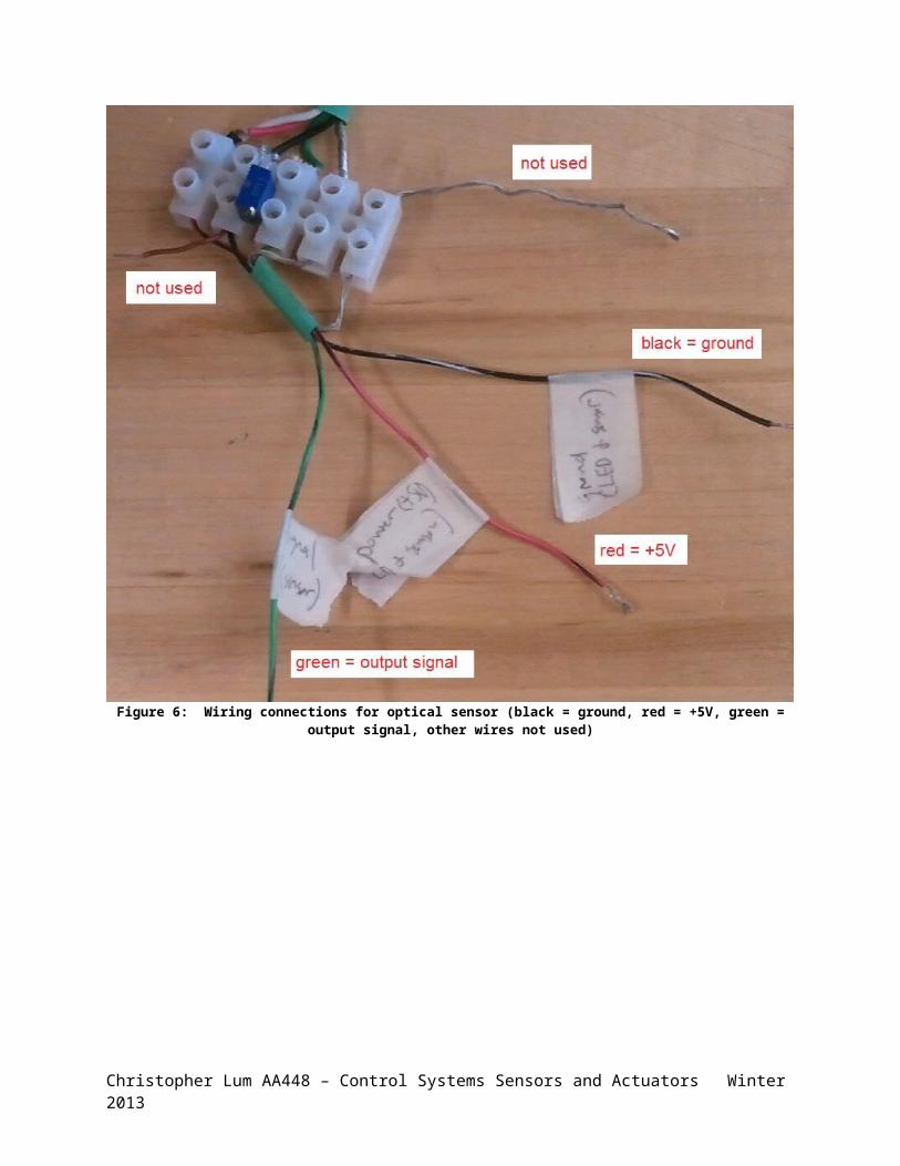
Figure 6: Wiring connections for optical sensor (black = ground, red = +5V, green = output signal, other wires not used)


Figure 7: Data from calibration of optical sensor used to generate a lookup table block in Simulink.

3. Calibration Stand Force Transducer

In this experiment, we determine how the output of the force transducer is related to the actual force applied to the transducer.

1. Ensure the apparatus is in the inverted position.2. Connect the force transducer to the calibration stand (Figure 8).3. Ensure that the force transducer is in the 10N range.4. Connect the force transducer to power and a multimeter (Figure 9).5. Weight the small metal pan assembly which is used to hold the weights.6. Attach the small metal pan assembly to the force transducer and place a known mass onto the

pan. Record the output voltage.8. Apply different masses to the system and record output voltages. Repeat for various masses to

generate a table similar to Table 3. 9. Use this data to a first order calibration curve between VT and force applied to transducer

(Figure 10). Be sure to account for the pan weight in your calibration.


a) Force transducer in free standing calibration state b) Force transducer on MBL calibration stand.Figure 8: Force transducer with small metal pan assembly and calibration weights.


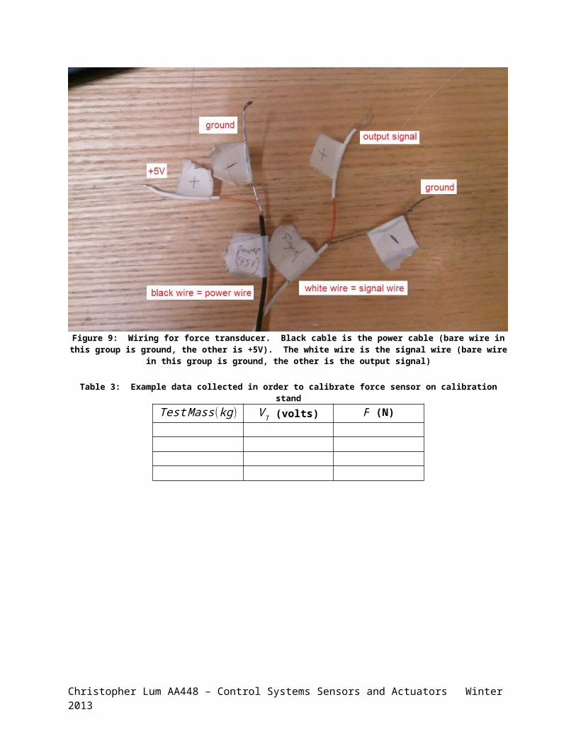
Figure 9: Wiring for force transducer. Black cable is the power cable (bare wire in this group is ground, the other is +5V). The white wire is the signal wire (bare wire in this group is ground, the other is the output signal)

Table 3: Example data collected in order to calibrate force sensor on calibration standTest Mass(kg) V T (volts) F (N)


Figure 10: Example calibration curve for force transducer.

4. Characterize Magnetic Force

In this experiment, we determine how the force applied by the magnet on the ball is a function of both the ball position and the voltage applied to the magnet.

1. Ensure the apparatus is in the inverted position.2. Weigh the ball and rod assembly.3. Connect the ball and rod assembly to the force transducer (Figure 11).4. Connect the force transducer to an available A/D channel and a multimeter.5. Connect the position sensor to another available A/D channel and a multimeter.6. Connect the Kepco amplifier to the magnet.7. Create a Simulink model which will

a. Apply a known, constant voltage to the Kepco amplifier, u.b. Measure output voltage from the position sensor, VD. c. Measure output voltage from the force transducer, VT .d. Sample data at a reasonable rate.

8. Retract the ball all the way.9. Set a constant voltage in the Simulink model and start recording data. Collect data for V m∈ [0,15 ] volts (use steps of 1 volt).


10. Slowly lower the ball until you get close to, but not touching, the tip of the magnet (do not let the ball get stuck to the magnet).

11. Slowly reverse the direction of the ball and bring it back to the fully retracted position.12. Stop recording data.13. Plot the data for this run and verify that it is reasonable (if not, try removing spikes and outliers).

Ensure that the values recorded by xPC target are the same as the values displayed on the multimeter. Repeat if necessary. You plot should be similar to Figure 12.

14. Save the data of u, VD , and VT for each run. Use this data to generate a series of curves similar to Figure 13.

15. Use methods described in lecture to characterize how the magnet force is a function of the ball position and magnet voltage, Fm ( z ,V m ).

Figure 11: Force transducer with ball and rod assembly (assembly is inverted).


Figure 12: Example data collected during single run

Figure 13: Example of calibrated magnetic force data (example data set is incomplete)


Stop: You have completed the operations for the first week of lab 3.


Evaluating Optical Sensor Calibration

In this section, you will verify that your calibration of the optical sensor is reasonable.

1. Create an xPC Simulink model which converts the output voltage from the optical sensor to a position (use the data you gathered and reduced from week 1).

2. Collect data with this model while moving the appropriately sized ball up and down from the tip of the magnet.

3. Plot the data and verify that it is reasonable.

Evaluating Trim Point Calculations

In this section, you will verify that your calculation of the trim voltage, u1 , o, is reasonable.

1. Set hardware limits on the Kepco amplifier output to the range of [-15,15] volts. Do not skip this step!

2. Hold the ball at your desired trim distance from the tip of the magnet.3. Create a Simulink model which sends a desired control signal, u(t ), to the Kepco (recall that u ( t )

is defined as the output from the D/A). Slowly increase the control voltage to the Kepco amplifier to verify that your calculation of u1 , o is reasonable.

4. Attempt to levitate the ball with by placing the Kepco in power supply mode and manually controlling the voltage knob. You will earn an instant 4.0 in this class if you are successful.

Attempt Bang/Bang Control

In this section, we will attempt to control this non-linear system with a simple bang/bang controller.

1. Attempt to stabilize the system with a simple bang/bang controller.2. Experiment with different “on” voltages.3. Do not spend too much time on this section as we do not anticipate this controller to be

successful.

Linearize System

In this section, you will generate a linear approximation of the system at the desired trim point.

1. Use techniques described in lecture to create a linear approximation of this system at the desired trim point.

2. Verify that the poles of this system predict an unstable system.


Position Control Via Full State Feedback

In this section, you will explore using full state feedback to design a position controller.

Pole Placement Technique1. Using methods described in class, create a full state feedback controller which does not saturate

the control signal and only requires position feedback (consider starting with desired closed loop poles around −60 ,−70.

2. Validate this controller with your non-linear simulation before attempting to implement this controller on the hardware.

3. Create a Simulink model which implements this controller on the hardware.4. Start the target application and slowly insert your ball into the magnetic field.5. Plot the response as the system is regulated to zero. Ensure that your controller does not

saturate.

LQR Technique1. Using methods described in class, create an LQR feedback controller which does not saturate

the control signal and only requires position feedback. Start with Q = diag([10 0]) and R = 0.00001.

2. Repeat the same experiment as the previous section.3. Investigate the behavior as R increases relative to Q.

Position Control Via PID

In this section, we explore designing a position controller for the motor using a proportional and derivative controller.

Proportional and Derivative Control Only1. Use your results from the full state feedback section to design a PD controller.2. Examine the root locus of your desired PD controller and modify your gains if desired.3. Test your PD controller with the system.

Informed PID Control1. Add a small integral gain to your controller to create a full PID controller.2. Verify that the root locus of your system is stable.3. Test your PID controller with the system.4. Evaluate the robustness of your controller by adding a second ball to the first.

Stop: You have completed the operations for week 2 of lab 3.


Items to Address in Report

An incomplete list of items to address in your lab write up include

Derivation, discussion, and results of obtaining model parameters from experimental resultso Comparison of motor inductance derivation using both time and frequency domain

approaches.o Actual motor friction and approximations

Simulation results and comparison of ODE, state space, and transfer function representations of system with experimental data.

Discussion of how P, I, and D components of control compose overall control system. Root locus of appropriate systems for position and velocity control. Analysis and discussion of practical implementations of PID and full state feedback controllers. Discussion regarding LQR and full state feedback controllers (pros/cons, open loop and closed

loop poles).


Bibliography


Validation

Levitators and test stands calibrated and verified on 02/22/13 with Robert Gordon

Levitator 1 2 3 4 5Optical Sensor YES YES YES YESMagnetic coil YES YES YES (no

ground)YES

Controller working

YES YES (gains might need adjusting)

YES YES

Calibration Stand 1 2Position Sensor YES YES

Load Cell 1 2Output Voltage YES YES


Abstract - University of Washingtonfaculty.washington.edu/lum/TEMP/aa448/lab_3_mbl.docx · Web...

Documents

Transcript of Abstract - University of Washingtonfaculty.washington.edu/lum/TEMP/aa448/lab_3_mbl.docx · Web...