ABSTRACT Title of Thesis: VEHICLE HANDLING, STABILITY, · ABSTRACT Title of Thesis: VEHICLE...
140
ABSTRACT Title of Thesis: VEHICLE HANDLING, STABILITY, AND BIFURCATION ANALYSIS FOR NONLINEAR VEHICLE MODELS Vincent Nguyen, Master of Science, 2005 Thesis directed by: Dr. Gregory A. Schultz Department of Mechanical Engineering Vehicle handling, stability, and bifurcation of equilibrium conditions were stud- ied using a state vector approach. The research provided a framework for an improved method of vehicle handling assessment that included non-linear regions of performance and transient behavior. Vehicle models under pure lateral slip, constant velocity, and constant front steer were developed. Four-wheel, two-axle vehicle models were evolved from simpler models and were extended to include ve- hicle roll dynamics and lateral load transfer effects. Nonlinearities stem from tire force characteristics that include tire force saturation. Bifurcations were studied by quasi-static variations of vehicle speed and front steer angle. System mod- els were expanded, assessing overall stability, including vehicle behavior outside normal operating ranges. Nonlinear models of understeering, oversteering, and
Transcript of ABSTRACT Title of Thesis: VEHICLE HANDLING, STABILITY, · ABSTRACT Title of Thesis: VEHICLE...

ABSTRACT
Title of Thesis: VEHICLE HANDLING, STABILITY,
AND BIFURCATION ANALYSIS
FOR NONLINEAR VEHICLE MODELS
Vincent Nguyen, Master of Science, 2005
Thesis directed by: Dr. Gregory A. Schultz
Department of Mechanical Engineering
Vehicle handling, stability, and bifurcation of equilibrium conditions were stud-
ied using a state vector approach. The research provided a framework for an
improved method of vehicle handling assessment that included non-linear regions
of performance and transient behavior. Vehicle models under pure lateral slip,
constant velocity, and constant front steer were developed. Four-wheel, two-axle
vehicle models were evolved from simpler models and were extended to include ve-
hicle roll dynamics and lateral load transfer effects. Nonlinearities stem from tire
force characteristics that include tire force saturation. Bifurcations were studied
by quasi-static variations of vehicle speed and front steer angle. System mod-
els were expanded, assessing overall stability, including vehicle behavior outside
normal operating ranges. Nonlinear models of understeering, oversteering, and

neutral steering vehicles were created and analyzed. Domains of attraction for sta-
ble equilibrium were discussed along with physical interpretations of results from
the system analysis.

VEHICLE HANDLING, STABILITY,
AND BIFURCATION ANALYSIS
FOR NONLINEAR VEHICLE MODELS
by
Vincent Nguyen
Thesis submitted to the Faculty of the Graduate School of theUniversity of Maryland, College Park in partial fulfillment
of the requirements for the degree ofMaster of Science
2005
Advisory Committee:
Dr. Gregory A. Schultz, Chairman/AdvisorProfessor Balakumar BalachandranProfessor David Holloway

c© Copyright by
Vincent Nguyen
2005
DEDICATION
To my father, who always allowed me to find my own path. Thank
you for your support in all of my endeavors.
ii

ACKNOWLEDGEMENTS
Thanks to: Dr. Greg Schultz for providing me with this amazing op-
portunity for research. And for his guidance, support and especially
his enthusiasm throughout the entire process. Dr. Balakumar Bal-
achandran, for his essential technical assistance, and for finding the
time to meet with me every week. His supervision and guidance made
this research possible. Ivan Tong at Aberdeen Test Center (ATC) for
his assistance in discussing and developing this work, and in particular
his vital intuitions that led to the expanded model. Kevin Kefauver
and the Roadway Simulator group at Aberdeen Test Center for their
assistance and data that supported this research.
Also thanks to Dr. David Holloway who introduced me to the exciting
field of automotive engineering which has not only led me to this work,
but has predominated my research, academic and personal interests for
the last four years.
Lastly, I’d like to thank Nicole Craver who has been by my side, my
best friend, for the last seven years. She has supported me in all things,
this work included. I could not have done it without her.
iii

TABLE OF CONTENTS
List of Tables vii
List of Figures viii
1 Introduction 1
1.1 SAE vehicle model . . . . . . . . . . . . . . . . . . . . . . . . . . . 4
1.2 Steady-state vehicle handling classification . . . . . . . . . . . . . . 5
1.3 State space, system stability, and phase portraits . . . . . . . . . . 10
1.4 Literature review . . . . . . . . . . . . . . . . . . . . . . . . . . . . 15
1.4.1 Handling classifications . . . . . . . . . . . . . . . . . . . . . 15
1.4.2 Stability notions . . . . . . . . . . . . . . . . . . . . . . . . 16
1.4.3 State space approaches . . . . . . . . . . . . . . . . . . . . . 17
1.5 Contributions and thesis organization . . . . . . . . . . . . . . . . . 17
2 Development of theoretical models 20
2.1 Bicycle model . . . . . . . . . . . . . . . . . . . . . . . . . . . . . . 20
2.1.1 Bifurcation in steer . . . . . . . . . . . . . . . . . . . . . . . 25
2.1.2 Bifurcation in velocity . . . . . . . . . . . . . . . . . . . . . 29
2.2 Tandem-axle model . . . . . . . . . . . . . . . . . . . . . . . . . . . 33
2.3 Four-wheel model . . . . . . . . . . . . . . . . . . . . . . . . . . . . 38
iv
3 LTV model 45
3.1 Tire Model . . . . . . . . . . . . . . . . . . . . . . . . . . . . . . . 46
3.1.1 The Magic Tire Formula . . . . . . . . . . . . . . . . . . . . 46
3.1.2 The genetic optimization algorithm . . . . . . . . . . . . . . 49
3.1.3 Results of the algorithm . . . . . . . . . . . . . . . . . . . . 53
3.1.4 Modified formulation . . . . . . . . . . . . . . . . . . . . . . 55
3.2 LTV four-wheel model results . . . . . . . . . . . . . . . . . . . . . 67
3.3 Expanded model . . . . . . . . . . . . . . . . . . . . . . . . . . . . 68
3.3.1 High-slip tire force model . . . . . . . . . . . . . . . . . . . 71
3.3.2 Expanded model homoclinic orbit generation . . . . . . . . . 74
3.3.3 Expanded model results . . . . . . . . . . . . . . . . . . . . 74
3.4 Lateral load transfer model . . . . . . . . . . . . . . . . . . . . . . . 78
3.4.1 Additional states . . . . . . . . . . . . . . . . . . . . . . . . 78
3.5 Lateral load model results . . . . . . . . . . . . . . . . . . . . . . . 82
4 Analysis and observations 86
4.1 Phase portraits . . . . . . . . . . . . . . . . . . . . . . . . . . . . . 86
4.2 Equilibrium points . . . . . . . . . . . . . . . . . . . . . . . . . . . 88
4.3 Bifurcation diagrams . . . . . . . . . . . . . . . . . . . . . . . . . . 92
4.4 Understeer and neutral steer . . . . . . . . . . . . . . . . . . . . . . 93
4.4.1 Understeer . . . . . . . . . . . . . . . . . . . . . . . . . . . . 94
4.4.2 Neutral steer . . . . . . . . . . . . . . . . . . . . . . . . . . 96
4.4.3 US/OS/NS bifurcation diagrams . . . . . . . . . . . . . . . 97
4.5 Expanded model results . . . . . . . . . . . . . . . . . . . . . . . . 102
4.5.1 General stability versus practical stability . . . . . . . . . . 102
4.5.2 Practicality of constant velocity assumptions . . . . . . . . . 108
v

4.6 Lateral load model . . . . . . . . . . . . . . . . . . . . . . . . . . . 109
4.7 Nonlinear steady-state handling classification . . . . . . . . . . . . . 109
5 Summary and recommendations for future work 117
5.1 Recommendations for future work . . . . . . . . . . . . . . . . . . . 118
Bibliography 120
vi

LIST OF TABLES
2.1 Bicycle model tire parameters. . . . . . . . . . . . . . . . . . . . . . 23
2.2 Tandem-axle bicycle model tire parameters. . . . . . . . . . . . . . 34
2.3 4 wheel model tire parameters. . . . . . . . . . . . . . . . . . . . . . 41
3.1 LTV lateral tire force data @ 20 psi. . . . . . . . . . . . . . . . . . 56
3.2 LTV lateral tire force data @ 35 psi. . . . . . . . . . . . . . . . . . 57
3.3 LTV lateral tire force data @ 50psi. . . . . . . . . . . . . . . . . . . 58
3.4 LTV GA coefficient results. . . . . . . . . . . . . . . . . . . . . . . 66
vii

LIST OF FIGURES
1.1 SAE vehicle coordinate orientations. . . . . . . . . . . . . . . . . . 4
1.2 SAE four-wheel vehicle parameters. The blue circle represents the
vehicle CG, β represents the vehicle sideslip, and δf represents the
front steer angle. . . . . . . . . . . . . . . . . . . . . . . . . . . . . 5
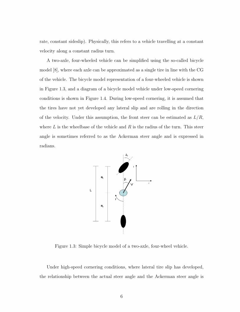
1.3 Simple bicycle model of a two-axle, four-wheel vehicle. . . . . . . . 6
1.4 Diagram of low-speed cornering with bicycle model. . . . . . . . . . 7
1.5 Tire force orientations for linear model used in [8] for classification
of US/OS/NS. . . . . . . . . . . . . . . . . . . . . . . . . . . . . . . 8
1.6 Handling diagram for US/OS/NS using linear tire model. . . . . . . 10
1.7 Handling diagram for nonlinear tire forces. . . . . . . . . . . . . . . 11
1.8 Spring-mass-damper system. . . . . . . . . . . . . . . . . . . . . . . 11
1.9 Phase portrait for simple spring-mass-damper system with m = 1,
k = 1, c = 1. . . . . . . . . . . . . . . . . . . . . . . . . . . . . . . . 14
2.1 Bicycle model presented in [18]. . . . . . . . . . . . . . . . . . . . . 21
2.2 SAE representation of bicycle model. . . . . . . . . . . . . . . . . . 22
2.3 Tire force diagram. . . . . . . . . . . . . . . . . . . . . . . . . . . . 23
2.4 Tire force versus slip angle for front and rear tires in bicycle model. 24
2.5 Phase portrait for bicycle model at δf = 0 radians and V = 20 m/s. 26
viii

2.6 Phase portrait for bicycle model at δf = 0.015 radians and V = 20
m/s. . . . . . . . . . . . . . . . . . . . . . . . . . . . . . . . . . . . 27
2.7 Phase portrait for bicycle model at δf = 0.030 radians and V = 20
m/s. . . . . . . . . . . . . . . . . . . . . . . . . . . . . . . . . . . . 27
2.8 Bicycle model bifurcation diagram. Equilibrium values of β versus
steer angle. . . . . . . . . . . . . . . . . . . . . . . . . . . . . . . . 28
2.9 Bicycle model bifurcation diagram. Equilibrium values of r versus
steer angle. . . . . . . . . . . . . . . . . . . . . . . . . . . . . . . . 28
2.10 Phase portrait for bicycle model at V = 10 m/s and δf = 0.015
radians. . . . . . . . . . . . . . . . . . . . . . . . . . . . . . . . . . 30
2.11 Phase portrait for bicycle model at V = 20 m/s and δf = 0.015
radians. . . . . . . . . . . . . . . . . . . . . . . . . . . . . . . . . . 30
2.12 Phase portrait for bicycle model at V = 20 m/s and δf = 0.015
radians. . . . . . . . . . . . . . . . . . . . . . . . . . . . . . . . . . 31
2.13 Bicycle model bifurcation diagram. Equilibrium values of β versus
velocity. . . . . . . . . . . . . . . . . . . . . . . . . . . . . . . . . . 31
2.14 Bicycle model bifurcation diagram. Equilibrium values of r versus
velocity. . . . . . . . . . . . . . . . . . . . . . . . . . . . . . . . . . 32
2.15 SAE representation of bicycle model for a tandem-axle vehicle. . . . 33
2.16 Phase portrait for tandem-axle model at V = 10 m/s and δf = 0.015
radians. . . . . . . . . . . . . . . . . . . . . . . . . . . . . . . . . . 35
2.17 Phase portrait for tandem-axle model at V = 25 m/s and δf = 0.015
radians. . . . . . . . . . . . . . . . . . . . . . . . . . . . . . . . . . 36
2.18 Phase portrait for tandem-axle model at V = 40 m/s and δf = 0.015
radians. . . . . . . . . . . . . . . . . . . . . . . . . . . . . . . . . . 36
ix
2.19 Bicycle model bifurcation diagram. Equilibrium values of β versus
front steer angle. . . . . . . . . . . . . . . . . . . . . . . . . . . . . 37
2.20 Bicycle model bifurcation diagram. Equilibrium values of r versus
front steer angle. . . . . . . . . . . . . . . . . . . . . . . . . . . . . 37
2.21 SAE representation of the 4 wheel model. . . . . . . . . . . . . . . . 38
2.22 Phase portrait for 4 wheel model at V = 10 m/s and δf = 0.015
radians. . . . . . . . . . . . . . . . . . . . . . . . . . . . . . . . . . 42
2.23 Phase portrait for 4 wheel model at V = 20 m/s and δf = 0.015
radians. . . . . . . . . . . . . . . . . . . . . . . . . . . . . . . . . . 42
2.24 Phase portrait for 4 wheel model at V = 30 m/s and δf = 0.015
radians. . . . . . . . . . . . . . . . . . . . . . . . . . . . . . . . . . 43
2.25 Bicycle model bifurcation diagram. Equilibrium values of β versus
speed. . . . . . . . . . . . . . . . . . . . . . . . . . . . . . . . . . . 43
2.26 Bicycle model bifurcation diagram. Equilibrium values of r versus
speed. . . . . . . . . . . . . . . . . . . . . . . . . . . . . . . . . . . 44
3.1 General Magic Tire Formula slip curve [19]. . . . . . . . . . . . . . 47
3.2 GA flowchart. . . . . . . . . . . . . . . . . . . . . . . . . . . . . . . 52
3.3 Genetic algorithm mean square error vs. iterations. . . . . . . . . . 54
3.4 Tire force vs. slip angle, GA results. . . . . . . . . . . . . . . . . . 54
3.5 LTV tire lateral force vs. slip angle at 20 psi. . . . . . . . . . . . . 56
3.6 LTV tire lateral force vs. slip angle at 35 psi. . . . . . . . . . . . . 57
3.7 LTV tire lateral force vs. slip angle at 50 psi. . . . . . . . . . . . . 58
3.8 Original GA results for lateral force at the highest vertical load
tested, performed for 20 runs at each tire pressure. . . . . . . . . . 60
x
3.9 GA results when holding C=1.3 for lateral force at the highest ver-
tical load tested, performed for 20 runs at each tire pressure. . . . . 60
3.10 Example of undesirable GA solution for 35 psi, C=1.3, E allowed
to float according to full tire model formulation. . . . . . . . . . . . 61
3.11 Example of undesirable GA solution for 50 psi, C=1.3, E allowed
to float according to full tire model formulation. . . . . . . . . . . . 61
3.12 Lateral force vs. vertical load for undesirable solution at 35 psi. . . 62
3.13 Lateral force vs. vertical load for undesirable solution at 50 psi. . . 62
3.14 Example of a desirable GA solution for 50 psi, C=1.3, E=optmized
constant. . . . . . . . . . . . . . . . . . . . . . . . . . . . . . . . . . 64
3.15 Lateral force vs. vertical load for desirable solution at 50 psi. . . . . 64
3.16 Lateral force vs. slip angle for 20 psi data. . . . . . . . . . . . . . . 65
3.17 Lateral force vs. slip angle for 35 psi data. . . . . . . . . . . . . . . 65
3.18 Phase portrait for LTV 4 wheel model at V = 10 m/s and δf = 0.015
radians. . . . . . . . . . . . . . . . . . . . . . . . . . . . . . . . . . 69
3.19 Phase portrait for LTV 4 wheel model at V = 27 m/s and δf = 0.015
radians. . . . . . . . . . . . . . . . . . . . . . . . . . . . . . . . . . 69
3.20 Phase portrait for LTV 4 wheel model at V = 36 m/s and δf = 0.015
radians. . . . . . . . . . . . . . . . . . . . . . . . . . . . . . . . . . 70
3.21 Bifurcation diagram for LTV 4 wheel model, equilibrium values of
β versus speed. . . . . . . . . . . . . . . . . . . . . . . . . . . . . . 70
3.22 Bifurcation diagram for LTV 4 wheel model, equilibrium values of
r versus speed. . . . . . . . . . . . . . . . . . . . . . . . . . . . . . 71
3.23 Tire force for “small” tire slip angle with force resolved perpendic-
ular to velocity direction. . . . . . . . . . . . . . . . . . . . . . . . . 72
xi

3.24 Tire force direction for 90◦ tire slip angle with force resolved per-
pendicular to velocity direction. . . . . . . . . . . . . . . . . . . . . 73
3.25 Tire force direction for 90◦ tire slip angle with force resolved per-
pendicular to tire heading. . . . . . . . . . . . . . . . . . . . . . . . 73
3.26 Wrapped tire lateral force function. . . . . . . . . . . . . . . . . . . 73
3.27 Expanded phase portrait for LTV 4 wheel model at V = 10 m/s
and δf = 0.015 radians. . . . . . . . . . . . . . . . . . . . . . . . . . 75
3.28 Expanded phase portrait for LTV 4 wheel model at V = 27 m/s
and δf = 0.015 radians. . . . . . . . . . . . . . . . . . . . . . . . . . 76
3.29 Expanded phase portrait for LTV 4 wheel model at V = 36 m/s
and δf = 0.015 radians. . . . . . . . . . . . . . . . . . . . . . . . . . 77
3.30 Vehicle roll axis. . . . . . . . . . . . . . . . . . . . . . . . . . . . . . 78
3.31 Unsprung mass free body diagram. . . . . . . . . . . . . . . . . . . 79
3.32 Sprung mass free body diagram. . . . . . . . . . . . . . . . . . . . . 80
3.33 Phase portrait for lateral load transfer model at V = 10 m/s and
δf = 0.015 radians. . . . . . . . . . . . . . . . . . . . . . . . . . . . 83
3.34 Phase portrait for lateral load transfer model at V = 25 m/s and
δf = 0.015 radians. . . . . . . . . . . . . . . . . . . . . . . . . . . . 84
3.35 Phase portrait for lateral load transfer model at V = 40 m/s and
δf = 0.015 radians. . . . . . . . . . . . . . . . . . . . . . . . . . . . 85
4.1 Vehicle orientation plot for a drift equilibrium point. . . . . . . . . 90
4.2 Vehicle orientation plot for equilibrium points of LTV model at 10
m/s. . . . . . . . . . . . . . . . . . . . . . . . . . . . . . . . . . . . 91
4.3 Vehicle orientation plot for equilibrium points of LTV model at 27
m/s. . . . . . . . . . . . . . . . . . . . . . . . . . . . . . . . . . . . 91
xii
4.4 Zoomed in view of bifurcation diagram for LTV 4 wheel model,
equilibrium values of β versus speed. . . . . . . . . . . . . . . . . . 93
4.5 Low speed, understeering phase plot. . . . . . . . . . . . . . . . . . 95
4.6 High speed, understeering phase plot. . . . . . . . . . . . . . . . . . 95
4.7 Low speed, neutral steering phase plot. . . . . . . . . . . . . . . . . 96
4.8 High speed, neutral steering phase plot. . . . . . . . . . . . . . . . . 97
4.9 Bifurcation diagram for LTV 4 wheel model, equilibrium values of
β versus speed. . . . . . . . . . . . . . . . . . . . . . . . . . . . . . 98
4.10 Bifurcation diagram for LTV 4 wheel model, equilibrium values of
r versus speed. . . . . . . . . . . . . . . . . . . . . . . . . . . . . . 99
4.11 β Speed bifurcation diagram for understeering model. . . . . . . . . 99
4.12 r Speed bifurcation diagram for understeering model. . . . . . . . . 100
4.13 β Speed bifurcation diagram for neutral steering model. . . . . . . . 100
4.14 r Speed bifurcation diagram for neutral steering model. . . . . . . . 101
4.15 Phase portrait for extended LTV model at V = 27 m/s. . . . . . . 103
4.16 Orientation plot for trajectory highlighted in V = 27 m/s phase plot.104
4.17 Phase portrait for extended LTV model at V = 36 m/s. . . . . . . 105
4.18 Orientation plot for trajectory highlighted in V = 36 m/s phase plot.106
4.19 Orientation plot for a rapidly spinning vehicle. . . . . . . . . . . . . 107
4.20 Normalized tire force for bicycle model. . . . . . . . . . . . . . . . . 114
4.21 Zoomed in view of normalized tire force forbicycle model. . . . . . . 114
4.22 (αr − αf ) versus normalized tire force for theoretical bicycle model. 115
4.23 Normalized tire force for LTV four-wheel model. . . . . . . . . . . . 115
4.24 (αr − αf ) versus normalized tire force for LTV four-wheel model. . . 116
xiii

5.1 Phase portrait with overlaying plot of stable equilibrium at several
other steer angles. Provided by ATC. . . . . . . . . . . . . . . . . . 118
xiv
Chapter 1
Introduction
Vehicle dynamics and stability have been of considerable interest to automotive
engineers, automobile manufacturers, the government, public safety groups, and
the general public for a number of years. The obvious dilemma is that people
naturally desire to drive faster and faster on the roads and highways, yet they
expect their vehicles to be “infinitely” stable and safe during all normal and emer-
gency maneuvers. For the most part, people pay little attention to the limited
handling potential of their vehicles until some unusual behavior is observed that
often results in fatality. Extreme examples of this are the handling behavior of
the Chevrolet Corvair in the 1960s and the recent rollovers experienced with the
Ford Explorer in the 1990s. Although there was much confusion about the exact
cause of the Explorer rollovers, since they seemed to in part be linked to a model
of Firestone tires, it is interesting that Ford soon lengthened the wheelbase of the
vehicle. Nonetheless, significant incidents occurred, resulting in public outcry for
improvement in safety. Note that the rates of speed at which drivers travel is rarely
mentioned by the public as a root cause.
The fundamentals of the physics of vehicle handling began to be explored in
earnest in the 1930s and 1940s by Olley et al. [15]. This work began by exploring
1
the basic behavior of pneumatic tires, which at the time were bias ply constructions.
Radial tires began to gain widespread use in the 1970s. These new tires behaved
somewhat differently, affecting vehicle behavior, and led to a rapid development of
speed-rated tires. Better tires made it more comfortable for drivers to travel even
faster. Consequently, interest in vehicle handling continued.
Recent efforts to better understand vehicle handling have demonstrated that
much is still to be learned and developed in this field as vehicles continue to
evolve. These efforts include cooperative work done by the major automobile
manufacturers through the Alliance of Automobile Manufacturers [2], rule-making
work and studies conducted by the National Highway Traffic Safety Administra-
tion (NHTSA), inspired by the rollover problems experienced with popular sport
utility vehicles (SUVs), and Light Tactical Vehicle (LTV) handling studies being
conducted by the U.S. Army.
The rapid success of sport utility vehicles in the U.S. has heightened interest
in related rollover problems. Though most of the rollovers were tripped by leaving
the roadway or hitting an obstacle, approximately 10% are unexplained and likely
related to vehicle handling behavior [5]. The relatively high center-of-gravity of
SUVs make them highly susceptible to rollover for any number of reasons. The
introduction of stability control systems in American cars has opened up many
new and exciting opportunities for vehicle dynamicists and controls engineers in
the field of vehicle handling and stability research. New questions have arisen,
such as how to identify a spin-out while it is happening, what to do to control the
behavior, and how to control the behavior without creating an additional safety
hazard, such as making the vehicle completely unresponsive. In any regard, the
field of vehicle handling and stability is perhaps more exciting and full of problems
2

to solve than ever.
Historically, vehicle handling has been studied predominately by first quanti-
fying the steady-state behavior of vehicles and then trying to relate steady-state
principles to transient dynamics. This is so because steady-state behavior is much
easier to visualize than transient dynamics, which are much more difficult to de-
scribe, let alone visualize. Performance within the linear region of modern tires,
usually from 0.3 to 0.4 g of lateral acceleration, is well understood and predictable
for steady-state maneuvers, and also, to some extent, in the transient case. How-
ever, tires are very non-linear beyond 0.4 g and eventually saturate with subsequent
degradation in lateral force capability. Combining complicated tire characteristics
with lateral weight transfer, differences in front/rear roll stiffness, suspension and
steering kinematics and compliance, and other factors make transient behavior
very difficult to describe and predict. The differential equations that describe
vehicle motion can be written in terms of a few key variables and parameters as
linear time-invariant systems. However, the variables and parameters used in these
equations are often highly non-linear.
This research, presents a way to visualize transient behavior over a broad set
of vehicle operating states. The work presented here helps bridge the gap between
steady-state handling principles and transient dynamics, and provides an interest-
ing way to visualize handling behavior, understand how changes in vehicle set-up
affect stability, and provide a better way to teach vehicle dynamics. Ideas for fu-
ture work to extend this research to possibly better characterize transient behavior
will be introduced. In this chapter, the basics of steady-state vehicle dynamics will
be presented, followed by discussion of how the system equations are typically de-
veloped. Finally, a brief literature review and introduction of the current research
3

will be given.
1.1 SAE vehicle model
Figure 1.1: SAE vehicle coordinate orientations.
Unless otherwise noted, this paper uses the standard Society of Automotive
Engineers (SAE) coordinate system shown in Figure 1.1 [8]. The vehicle’s positive
x axis is defined to be along the forward direction of the vehicle’s longitudinal axis.
The y axis is defined to be towards the right-hand side of the vehicle (while facing
forward) and the z axis points in the downward direction. A two-axle, four-wheel
vehicle with front wheel steering making a right-hand turn is shown in Figure 1.2.
Also shown are the orientations of key vehicle parameters used in this research.
The green line denotes the path of the vehicle center of gravity (CG), shown as
a blue circle. The vehicle’s instantaneous velocity, V , is shown tangent to the
vehicle path. Vehicle sideslip, β, is defined as the angle between the vehicle x axis
and the velocity vector at the CG, with positive sideslip defined with the vehicle
axis oriented to the left of velocity. Front steer angle, δf , is the angle between the
centerline of the front tires and the vehicle x axis. Positive steer is achieved with
4

the wheels steered to the right. Vehicle yaw rate, r is defined as a positive rotation
about the vehicle z axis.
Figure 1.2: SAE four-wheel vehicle parameters. The blue circle represents the
vehicle CG, β represents the vehicle sideslip, and δf represents the front steer
angle.
1.2 Steady-state vehicle handling classification
Vehicle handling behavior is predominantly classified using the so-called understeer
(US), oversteer (OS), and neutral steer (NS) conditions. These terms are tradi-
tionally applied to steady-state handling conditions. Steady-state handling can
be defined as a maneuver in which there are constant vehicle parameters (steer
angle, velocity, roll angle, etc.) and the vehicle motion is constant (constant yaw
5
rate, constant sideslip). Physically, this refers to a vehicle travelling at a constant
velocity along a constant radius turn.
A two-axle, four-wheeled vehicle can be simplified using the so-called bicycle
model [8], where each axle can be approximated as a single tire in line with the CG
of the vehicle. The bicycle model representation of a four-wheeled vehicle is shown
in Figure 1.3, and a diagram of a bicycle model vehicle under low-speed cornering
conditions is shown in Figure 1.4. During low-speed cornering, it is assumed that
the tires have not yet developed any lateral slip and are rolling in the direction
of the velocity. Under this assumption, the front steer can be estimated as L/R,
where L is the wheelbase of the vehicle and R is the radius of the turn. This steer
angle is sometimes referred to as the Ackerman steer angle and is expressed in
radians.
Figure 1.3: Simple bicycle model of a two-axle, four-wheel vehicle.
Under high-speed cornering conditions, where lateral tire slip has developed,
the relationship between the actual steer angle and the Ackerman steer angle is
6

Figure 1.4: Diagram of low-speed cornering with bicycle model.
typically used to classify US/OS/NS for steady-state handling. For a high-speed
right-hand turn, an understeering vehicle will have a front steer angle that is greater
than the Ackerman steer angle. An oversteering vehicle will exhibit a lower steer
angle than the Ackerman steer angle, and a neutral steering vehicle maintains the
Ackerman steer angle through the high speed turns.
US/OS/NS can be described analytically. The tire force orientation for the
US/OS/NS classification used by Gillespie [8] is shown in Figure 1.5. Tire lateral
force is labelled as F and the tire slip angle, α, is defined as the angle between
the velocity at the tire and the heading of the tire. Using the bicycle model
under steady-state cornering in the positive yaw direction (right-hand turn), an
expression for front steer angle can be developed (Eq. (1.1)). The terms αf and
αr represent the front and rear tire slip angles. If in the maneuver, the front slip
angle is greater than the rear, the subsequent front steer angle is greater than
the Ackerman steer angle and the vehicle exhibits understeer. Conversely, if the
rear slip angle is greater than the front, the steer angle is less than the Ackerman
7

steer angle and the vehicle exhibits oversteer. If the slip angles are equal, then the
vehicle is steering at the Ackerman steer angle and is exhibiting neutral steer.
δf =L
R+ αf − αr (1.1)
Figure 1.5: Tire force orientations for linear model used in [8] for classification of
US/OS/NS.
Gillespie takes the analysis further with the use of a linear tire force model.
Tire lateral force is assumed to be a linear function of the slip angle, and F = Cα ·α
describes the relationship. The coefficient Cα is called the tire-cornering stiffness
and is a property of the tire. The tire model can then be applied along with a force
balance equation to provide another expression for front steer angle, Eq. (1.2) [8].
Wf and Wr are the vehicle weights at the front and rear axles. In this expression,
if(
Wf
Cαf− Wr
Cαr
)is equal to 0, the vehicle is always neutral steering. However, if(
Wf
Cαf− Wr
Cαr
)is positive, front steer angle can be expected to be greater than the
Ackerman steer angle (at any given positive speed). In addition, the steer angle
can be expected to continue to increase with respect to increasing vehicle speed.
This means that the vehicle not only exhibits understeer, but it exhibits terminal
understeer (increasing steer angle) as the vehicle speed is increased. Similarly
8

when(
Wf
Cαf− Wr
Cαr
)is negative, the front steer angle will always be less than the
Ackerman angle (for positive velocity), and it will continue to decrease as vehicle
speed is increased. This vehicle not only exhibits oversteer, but exhibits terminal
oversteer as the velocity is increased.
δf =L
R+
(Wf
Cαf
− Wr
Cαr
)V 2
gR(1.2)
A handling diagram for the linear tire model and vehicle driving on a constant
radius is provided in Figure 1.6. Steer angle is plotted against lateral acceleration
(V 2/Rg). A neutral steering vehicle will maintain a constant steer angle (the
Ackerman steer angle). An understeering vehicle produces steer angles greater
than the Ackerman steer angle for nonzero velocity and will continue to increase
steer angle at a rate proportional to the lateral acceleration. An oversteering vehicle
operates at a steer angle less than the Ackerman steer angle and will decrease steer
angle at a rate proportional to the lateral acceleration.
In practice, during a maneuver, the operator has no notion of the Ackerman
steer angle. Instead, the operator perceives a change in steer angle as velocity
is increased or decreased. In addition, because of nonlinear tire responses, some
vehicles initially understeer, but as lateral acceleration is increased, a transition
to neutral steer and eventually oversteer occurs. Consequently, it may be more
practical from a driver’s point of view to think of the onset of neutral steer and
oversteer as occurring when the required steer angle to negotiate the turn begins
to decrease (as speed is increased).
As such, the commonly accepted relationship between the actual steer angle
and the Ackerman steer angle (greater than or less than) may not be descriptive
enough. For practical use, US/OS/NS should be defined by the slope of the steer
angle/acceleration curve rather than just the value of the steer angle (as compared
9

to the Ackerman steer angle). With the linear tire model, the relationship to the
no-slip (Ackerman) steer angle coincides with rate of change of the steer angle (if
δ > L/R then δ is always increasing and vice versa), so there is no distinction
between the two definitions. With nonlinear tire models, this is not necessarily the
case and a distinction must be made. In Figure 1.7, a typical handling diagram
for a heavy truck is shown. Notice how the vehicle transitions from understeer
to oversteer. The transition point occurs well before the steer angle drops below
the Ackerman angle. US/OS/NS within the nonlinear tire force regions will be
discussed later in this thesis.
Figure 1.6: Handling diagram for US/OS/NS using linear tire model.
1.3 State space, system stability, and phase por-
traits
The models used in this research are presented in state-space format. System states
are the essential parameters required to describe the system dynamics. Further-
more, all of the systems presented are autonomous, meaning that the governing
10
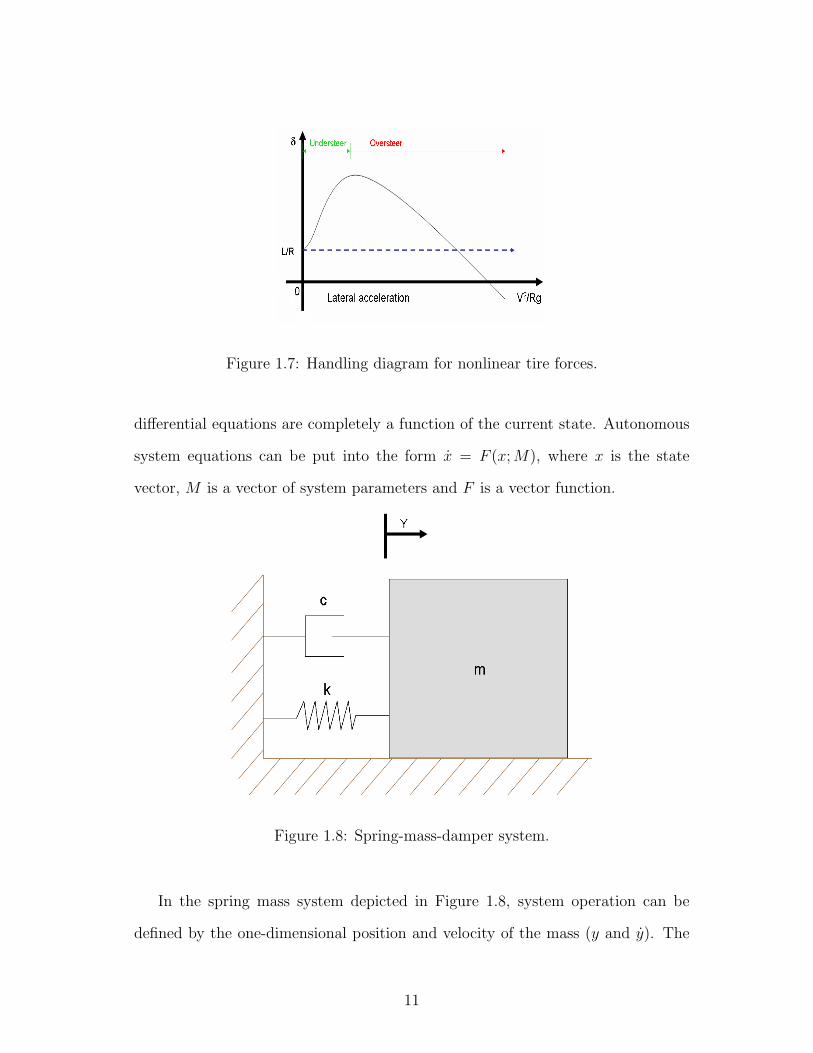
Figure 1.7: Handling diagram for nonlinear tire forces.
differential equations are completely a function of the current state. Autonomous
system equations can be put into the form x = F (x; M), where x is the state
vector, M is a vector of system parameters and F is a vector function.
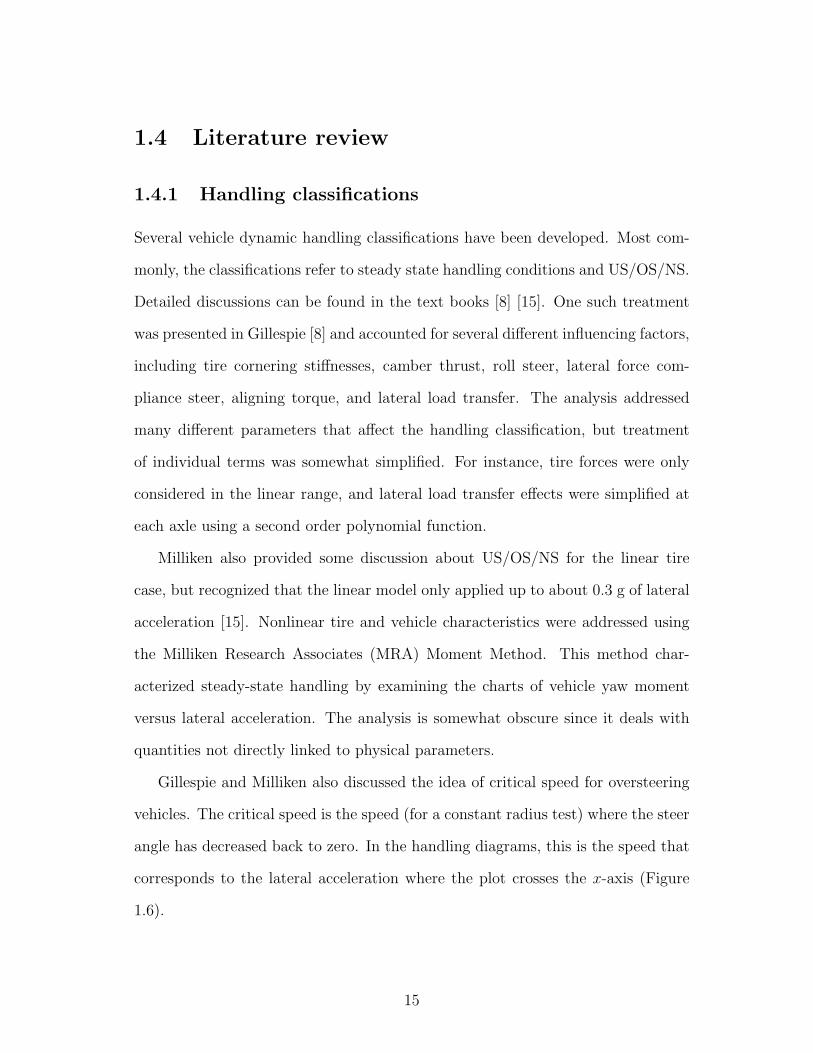
Figure 1.8: Spring-mass-damper system.
In the spring mass system depicted in Figure 1.8, system operation can be
defined by the one-dimensional position and velocity of the mass (y and y). The
11

state vector x can be defined as in Eq. (1.3). The governing equation for the
unforced system is shown in Eq. (1.4). This represents an autonomous system,
since the governing equation is expressed in state space as in Eq. (1.5), where M
is a vector of the system parameters (m, c, and k), and the vector function F is
defined according to Eq. (1.6).
x =
y
y
(1.3)
my + cy + ky = 0 (1.4)
x =
y
y
= F (x; M) (1.5)
F (x; M) =
y
(−ky − cy)/m
(1.6)
Equilibrium solutions in state space refer to solutions where the states hold
steady through time. In analytic terms, an equilibrium solution, x0, is a state
where the rate of change of the state vector x0 = F (x0; M) = 0. The local
stability of an equilibrium solution can be determined by observing the behavior
of the linearized vector function F at the equilibrium solution [17]. If the state
vector x has n dimensions, x can be expressed as x = [x1, x2, x3, · · · , xn] and F
as F = [F1, F2, F3, · · · , Fn], where Fi = xi ∀ i ∈ Z, 1 ≤ i ≤ n. Linearization
is accomplished by first determining the Jacobian matrix, A, which is defined as
A = DxF (x; M) at x = x0, where DxF (x; M) is defined by Eq. (1.7). If the
eigenvalues of the Jacobian matrix A have all nonzero real parts, the equilibrium
point, x0 is considered to be hyperbolic. For a hyperbolic equilibrium point, if all
the eigenvalues have negative real parts, then all local perturbations away from
the equilibrium solution, x0, decay with time and the solution is stable. If one or
12

more of the eigenvalues of A have positive real parts, then perturbations in some
directions away from x0 will increase with time and the solution is unstable. If
an unstable point has some eigenvalues with negative real parts and the rest with
positive real parts, perturbations away from x0 in certain directions will decay
while perturbations in other directions will increase, and the solution is called a
saddle point [17].
For the simple spring-mass-damper example, the equilibrium solution can be
found by solving F (x; M) = 0. The only equilibrium solution is y = 0, y = 0.
The Jacobian matrix can be defined according to Eq. (1.8). The eigenvalues at
x0 =
0
0
can be shown to always be negative for positive values of m, k, and
c. Therefore, x0 can be considered locally stable (and globally stable since the
system is linear). Another way to visualize this is to look at a phase portrait of
the system. Figure 1.9 is a phase portrait of the spring-mass-damper system with
m = 1, k = 1, and c = 1. The phase portrait is a graphical representation of
the state space, with the abscissa as the velocity value (y) and the ordinate as
the position value (y). The trajectories shown in blue represent the evolution of
the states from the initial conditions (represented by the red x’s) for velocity and
position. The phase portrait clearly shows that trajectories initiated throughout
the phase plane are attracted to the equilibrium point at (0, 0). This demonstrates
the stability of the solution, since perturbations away from the equilibrium point
will propagate back toward the equilibrium point. Phase portraits can be used
as visualization tools to describe system state progression and assess qualitative
13

stability, and will be used throughout this research.
DxF (x; M) =
∂F1
∂x1
∂F1
∂x2· · · ∂F1
∂xn
∂F2
∂x1
∂F2
∂x2· · · ∂F2
∂xn
......
. . ....
∂Fn
∂x1
∂Fn
∂x2· · · ∂Fn
∂xn
(1.7)
A = DxF (x; M) =
0 1
−k/m −c/m
(1.8)
Figure 1.9: Phase portrait for simple spring-mass-damper system with m = 1,
k = 1, c = 1.
14
1.4 Literature review
1.4.1 Handling classifications
Several vehicle dynamic handling classifications have been developed. Most com-
monly, the classifications refer to steady state handling conditions and US/OS/NS.
Detailed discussions can be found in the text books [8] [15]. One such treatment
was presented in Gillespie [8] and accounted for several different influencing factors,
including tire cornering stiffnesses, camber thrust, roll steer, lateral force com-
pliance steer, aligning torque, and lateral load transfer. The analysis addressed
many different parameters that affect the handling classification, but treatment
of individual terms was somewhat simplified. For instance, tire forces were only
considered in the linear range, and lateral load transfer effects were simplified at
each axle using a second order polynomial function.
Milliken also provided some discussion about US/OS/NS for the linear tire
case, but recognized that the linear model only applied up to about 0.3 g of lateral
acceleration [15]. Nonlinear tire and vehicle characteristics were addressed using
the Milliken Research Associates (MRA) Moment Method. This method char-
acterized steady-state handling by examining the charts of vehicle yaw moment
versus lateral acceleration. The analysis is somewhat obscure since it deals with
quantities not directly linked to physical parameters.
Gillespie and Milliken also discussed the idea of critical speed for oversteering
vehicles. The critical speed is the speed (for a constant radius test) where the steer
angle has decreased back to zero. In the handling diagrams, this is the speed that
corresponds to the lateral acceleration where the plot crosses the x-axis (Figure
1.6).
15
Karnopp briefly tackled the issue of nonlinear tire forces in the US/OS/NS
classification [10]. A similar method is presented later in this thesis. Karnopp also
mentioned the capability of a vehicle to exhibit different US/OS behavior at or
near limit conditions, depending on the tire saturation rates [10].
1.4.2 Stability notions
Handling classifications allow for stability limit definitions. For instance, US/OS/NS
can be quantified using understeer and oversteer gradients (slope of handling dia-
gram) [8] [15], and quantifiable limits can be defined. Gillespie uses critical speed
(where the vehicle has turned back to zero steer) for oversteering vehicles as a
stability limit [8].
Milliken provided some additional stability discussions using the linear vehicle
model. The stability of steady-state operation was evaluated for US/OS/NS ve-
hicles with respect to step sideslip inputs (at 0 steer). Also, steady-state stable
operating conditions were calculated using the linear bicycle model for particular
steer angles and sideslip values. This type of analysis is relatively simple for a
linear system, since steer angle and sideslip can be directly superimposed to define
overall tire forces. In the nonlinear case, Milliken’s Moment Method was developed
to determine steady-state operating conditions given a particular steer angle and
sideslip.
A numeric bifurcation analysis is presented in [4] that studies the hunting mo-
tions of rail vehicles. Hopf bifurcations [17] and limit cycle stability are examined
for railcars with four- and two-axle bogies, resulting in a simple bifurcation model
that relates the onset of stable limit cycles (hunting motions) to vehicle speed.
Stability limits are also required to define loss of vehicle control during tran-
16

sient field testing procedures. Forkenbrock, in [6], presented a NHTSA-developed
standard to define a spinout during a sine steer maneuver. Spinout or loss of vehi-
cle control is defined using yaw rate drop-off following a maneuver. After the steer
maneuver, if the vehicle yaw rate is not reduced to a percentage of the maximum
within a certain time, a loss of control is determined.
1.4.3 State space approaches
Interestingly enough, little work has been done with vehicle stability using a state
space system. For constant vehicle parameters, the state space vehicle models are
time invariant systems. Karnopp used a state space approach to study the stability
of a linear vehicle system (bicycle model with linear tire forces) [10]. Steady-
state dynamic equilibrium solutions were calculated and the stability of dynamic
equilibrium solutions were also assessed directly by linear stability methods.
Ono et al. presented a similar state space model in [18]. This model instead
used nonlinear tire forces. Stability was briefly assessed, and changes in the stable
solutions with respect to steer angle were studied. A front steer controller was
also proposed that intended to keep the nonlinear system stable while maneuver-
ing. Nevertheless, Ono’s work was fairly brief and simplified in terms of stability
analysis, since the focus of the work was on control.
1.5 Contributions and thesis organization
The main contributions of this thesis are the following:
• The nonlinear bicycle model for stability analysis presented in [18] was ex-
tended to include tandem-axle vehicle dynamics and independent four-wheel
17

dynamics.
• Bifurcations of equilibria were shown to occur with respect to vehicle velocity,
in addition to steer angle.
• A Light Tactical Vehicle (LTV) four-wheel model was created, which in-
cluded the development of a nonlinear tire model generated from limited
experimental tire data.
• The vehicle model was extended to study operations beyond normal operat-
ing limits. This allowed analysis of overall system stability characteristics.
• A lateral load transfer model was also presented. This model included roll
dynamics and tire force propagation.
• A detailed discussion about the physical insights and practical applications
of the analysis are provided.
• A presentation of US/OS/NS for nonlinear tire models was created and is
presented along with analysis results for US/OS/NS vehicles.
The rest of this thesis is organized as follows:
Chapter 2: In this chapter, all vehicle models are presented, beginning with
the original model provided in [18]. Bifurcations, or qualitative changes in the
phase portraits, are shown as front steer angle is varied. Similar bifurcations
involving the loss of stable equilibrium solutions are demonstrated with respect to
velocity as the control parameter. The model is then extended for use with tandem-
axle vehicles. Model parameters were adjusted to provide similar results as with
the two-axle bicycle model. An independent four-wheel (non-bicycle) model is
18

then presented for a two-axle vehicle. Advantages are discussed, and results for
the four-axle case are shown.
Chapter 3: In this chapter, the creation of a vehicle-based LTV model is
outlined. A tire model is first developed using a semi-empirical formulation along
with a genetic optimization algorithm. Four-wheel LTV model results obtained
with the new tire model are presented. The model is then expanded to allow for
accurate results at broader operating ranges. Domains of attraction for stable
points are also studied. Lateral load and roll dynamics are discussed, and a lateral
load LTV model is developed and results are presented.
Chapter 4: In this chapter, the physical insights gained from the analysis
are discussed. The practical meanings of the phase portraits and the equilibrium
solutions are discussed, as well as the domains of attraction for the stable points.
Bifurcation diagrams with respect to steer angle and the velocity are investigated
and tied to physical behavior. The expanded phase portraits are discussed in terms
of practical stability and analytical system stability. US/OS/NS classifications are
presented for nonlinear vehicle models, and US/NS/OS vehicles are studied using
the nonlinear analysis. Lateral load model results are also examined.
Chapter 5: Concluding remarks along with suggestions for future work are
collected and presented in this chapter.
19

Chapter 2
Development of theoretical models
In this chapter, an effort is made to systematically describe the basic concepts and
stability and bifurcation analysis techniques presented in this thesis. First, earlier
work by Ono et al. [18] is reproduced for a bicycle model of a two-axle vehicle to
explain and develop the basic concepts. Then, the simple bicycle model is extended
to tandem rear-axle vehicles. Finally, a four-wheel vehicle model and associated
analysis is presented, neglecting lateral weight transfer and roll dynamics. In
Chapter 3, a case study is presented for a four-wheel general purpose utility vehicle,
using real tire data. This new model is further developed to include lateral weight
transfer and roll dynamics. A detailed discussion of physical insights and the utility
of this stability approach is given in Chapter 4.
2.1 Bicycle model
The bifurcation analysis presented by Ono et al. [18] was based on a simple
“bicycle” model. In this approach, the actual forces acting on the vehicle are
approximated by modelling each axle as a single unit (single wheel). As such,
individual tire slip angles or individual tire loading during cornering, were not
20
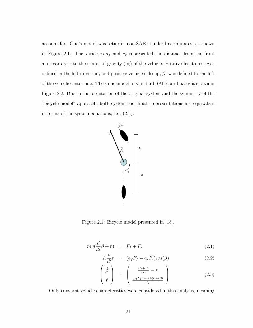
account for. Ono’s model was setup in non-SAE standard coordinates, as shown
in Figure 2.1. The variables af and ar represented the distance from the front
and rear axles to the center of gravity (cg) of the vehicle. Positive front steer was
defined in the left direction, and positive vehicle sideslip, β, was defined to the left
of the vehicle center line. The same model in standard SAE coordinates is shown in
Figure 2.2. Due to the orientation of the original system and the symmetry of the
”bicycle model” approach, both system coordinate representations are equivalent
in terms of the system equations, Eq. (2.3).
Figure 2.1: Bicycle model presented in [18].
mv(d
dtβ + r) = Ff + Fr (2.1)
Izd
dtr = (afFf − arFr)cos(β) (2.2) β
r
=
Ff+Fr
mv− r
(af Ff−arFr)cos(β)
Iz
(2.3)
Only constant vehicle characteristics were considered in this analysis, meaning
21

Figure 2.2: SAE representation of bicycle model.
there was no acceleration in the direction of the velocity and the front steer angle,
δf , remained constant. Motion was described with two states: β, representing
vehicle sideslip and r, representing vehicle yaw rate.
In this formulation, the overall axle forces (Ff and Fr) are defined in a direction
perpendicular to vehicle velocity at the cg. The ”bicycle model” approach treated
each axle as a single tire with a single slip angle. Axle forces were calculated
using an empirical tire formula, which was a simplified general form of the well
known “magic tire formula” [19]. The tire equation used by Ono et al. is shown in
Eq. (2.4). The slip angle, α, and the direction of the force were defined according
to Figure 2.3. The parameters B, C, D, and E were all constant parameters based
on empirical tire data, with slip angles as the only variable. The parameters used
for the front and rear tires were different, accounting for the tires themselves as
well as suspension setup and the weight distribution effects. A list the coefficients
22

used are shown in Table 2.1. In Figure 2.4 the tire force versus slip angle diagrams
are shown for the front and rear tires. Note that the nonlinear characteristics of
the tires prior to, during and after saturation were represented.
F = D · sin[C · tan−1
{B · α− E ·
(B · x− tan−1(B · α)
)}](2.4)
Figure 2.3: Tire force diagram.
Table 2.1: Bicycle model tire parameters.
B C D E
Front 11.275 1.56 -2574.7 -1.999
Rear 18.631 1.56 -1749.7 -1.7908
Slip angles at each of the tires were calculated by resolving the i and j com-
ponents of the velocity vectors based on the vehicle coordinate system, as shown
in Eqs. (2.5) and (2.6). The vehicle was assumed to be rigid in the yaw direction.
Eqs. (2.7), (2.8), (2.9), and (2.10) give the front and rear slip angles of the states.
23
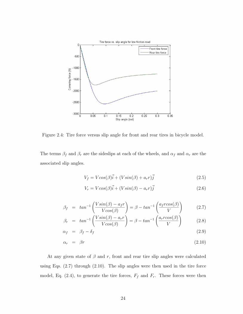
Figure 2.4: Tire force versus slip angle for front and rear tires in bicycle model.
The terms βf and βr are the sideslips at each of the wheels, and αf and αr are the
associated slip angles.
Vf = V cos(β)~i + (V sin(β) + arr)~j (2.5)
Vr = V cos(β)~i + (V sin(β)− arr)~j (2.6)
βf = tan−1
(V sin(β)− afr
V cos(β)
)= β − tan−1
(afrcos(β)
V
)(2.7)
βr = tan−1
(V sin(β)− arr
V cos(β)
)= β − tan−1
(arrcos(β)
V
)(2.8)
αf = βf − δf (2.9)
αr = βr (2.10)
At any given state of β and r, front and rear tire slip angles were calculated
using Eqs. (2.7) through (2.10). The slip angles were then used in the tire force
model, Eq. (2.4), to generate the tire forces, Ff and Fr. These forces were then
24
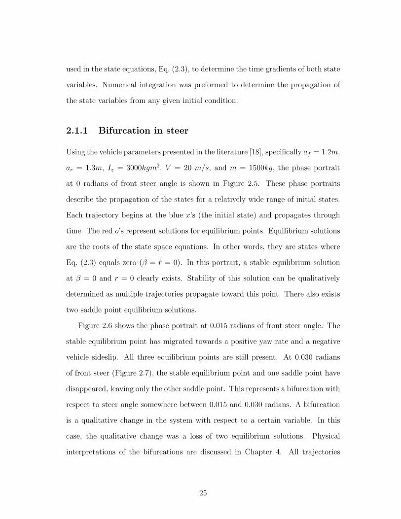
used in the state equations, Eq. (2.3), to determine the time gradients of both state
variables. Numerical integration was preformed to determine the propagation of
the state variables from any given initial condition.
2.1.1 Bifurcation in steer
Using the vehicle parameters presented in the literature [18], specifically af = 1.2m,
ar = 1.3m, Iz = 3000kgm2, V = 20 m/s, and m = 1500kg, the phase portrait
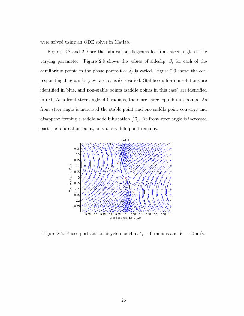
at 0 radians of front steer angle is shown in Figure 2.5. These phase portraits
describe the propagation of the states for a relatively wide range of initial states.
Each trajectory begins at the blue x’s (the initial state) and propagates through
time. The red o’s represent solutions for equilibrium points. Equilibrium solutions
are the roots of the state space equations. In other words, they are states where
Eq. (2.3) equals zero (β = r = 0). In this portrait, a stable equilibrium solution
at β = 0 and r = 0 clearly exists. Stability of this solution can be qualitatively
determined as multiple trajectories propagate toward this point. There also exists
two saddle point equilibrium solutions.
Figure 2.6 shows the phase portrait at 0.015 radians of front steer angle. The
stable equilibrium point has migrated towards a positive yaw rate and a negative
vehicle sideslip. All three equilibrium points are still present. At 0.030 radians
of front steer (Figure 2.7), the stable equilibrium point and one saddle point have
disappeared, leaving only the other saddle point. This represents a bifurcation with
respect to steer angle somewhere between 0.015 and 0.030 radians. A bifurcation
is a qualitative change in the system with respect to a certain variable. In this
case, the qualitative change was a loss of two equilibrium solutions. Physical
interpretations of the bifurcations are discussed in Chapter 4. All trajectories
25
were solved using an ODE solver in Matlab.
Figures 2.8 and 2.9 are the bifurcation diagrams for front steer angle as the
varying parameter. Figure 2.8 shows the values of sideslip, β, for each of the
equilibrium points in the phase portrait as δf is varied. Figure 2.9 shows the cor-
responding diagram for yaw rate, r, as δf is varied. Stable equilibrium solutions are
identified in blue, and non-stable points (saddle points in this case) are identified
in red. At a front steer angle of 0 radians, there are three equilibrium points. As
front steer angle is increased the stable point and one saddle point converge and
disappear forming a saddle node bifurcation [17]. As front steer angle is increased
past the bifurcation point, only one saddle point remains.
Figure 2.5: Phase portrait for bicycle model at δf = 0 radians and V = 20 m/s.
26

Figure 2.6: Phase portrait for bicycle model at δf = 0.015 radians and V = 20
m/s.
Figure 2.7: Phase portrait for bicycle model at δf = 0.030 radians and V = 20
m/s.
27

Figure 2.8: Bicycle model bifurcation diagram. Equilibrium values of β versus
steer angle.
Figure 2.9: Bicycle model bifurcation diagram. Equilibrium values of r versus
steer angle.
28
2.1.2 Bifurcation in velocity
A similar bifurcation analysis was done in this research with velocity as the control
parameter. Setting δf to 0.015, the velocity (V ) was varied. Figure 2.10 shows
the phase portrait at V = 10 m/s. As before, trajectories begin at the blue x’s
and propagate through time. Equilibrium points are designated as red o’s. At
δf = 0 and V = 10 m/s there exists the three equilibrium points, as before. At the
same steer angle with velocity increased to 20 m/s, the equilibrium points begin to
migrate (Figure 2.11). As velocity is increased further, a bifurcation (similar to the
one seen with increased steer angle) occurs. Figure 2.12 shows the phase portrait
at V = 30 m/s. The stable and one saddle node equilibrium point converged
and disappeared, leaving only the other saddle node equilibrium point. Figures
2.13 and 2.14, are the bifurcation diagrams with velocity as the control parameter.
Again the red points designate unstable equilibrium points and the blue points are
stable.
29

Figure 2.10: Phase portrait for bicycle model at V = 10 m/s and δf = 0.015
radians.
Figure 2.11: Phase portrait for bicycle model at V = 20 m/s and δf = 0.015
radians.
30

Figure 2.12: Phase portrait for bicycle model at V = 20 m/s and δf = 0.015
radians.
Figure 2.13: Bicycle model bifurcation diagram. Equilibrium values of β versus
velocity.
31
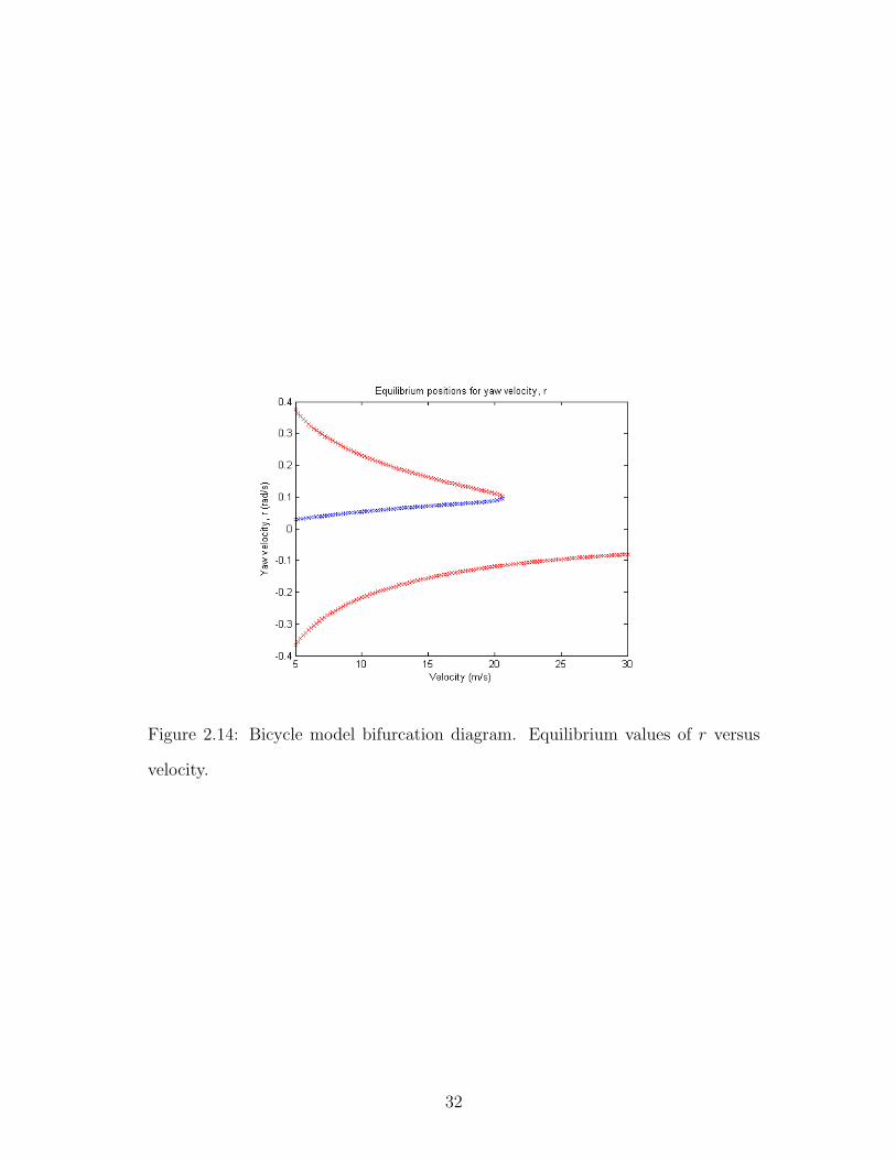
Figure 2.14: Bicycle model bifurcation diagram. Equilibrium values of r versus
velocity.
32
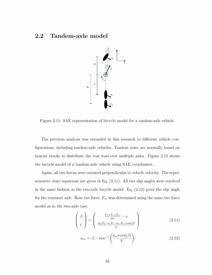
2.2 Tandem-axle model
Figure 2.15: SAE representation of bicycle model for a tandem-axle vehicle.
The previous analysis was extended in this research to different vehicle con-
figurations, including tandem-axle vehicles. Tandem axles are normally found on
heavier trucks to distribute the rear load over multiple axles. Figure 2.15 shows
the bicycle model of a tandem-axle vehicle using SAE coordinates.
Again, all tire forces were oriented perpendicular to vehicle velocity. The repre-
sentative state equations are given in Eq. (2.11). All tire slip angles were resolved
in the same fashion as the two-axle bicycle model. Eq. (2.12) gives the slip angle
for the rearmost axle. Rear tire force, Frr was determined using the same tire force
model as in the two-axle case. β
r
=
Ff+Fr+Frr
mv− r
(af Ff−arFr−arrFrr)cos(β)
Iz
(2.11)
αrr = β − tan−1
(arrrcos(β)
V
)(2.12)
33

For the numerical analysis, the tandem-axle vehicle was based on the previous
two-axle model in terms of vehicle parameters. This was done for comparison
and validation of the model results. The distance from the center of gravity to the
rearmost axle, arr, was set to 1.6m. Initially, the rear tire force parameters from the
two-axle model were used for both tandem axles. However, rear force saturation
was not evident, since effective rear force was doubled (the rear stabilizing moment
was more than doubled). Consequently, the original tire data was altered by
halving the scaling term D for both the rear axles. This allowed overall magnitude
for each tire to be scaled down while maintaining curve shape. Table 2.2 shows
the new parameters used for the tires in the tandem-axle model.
Table 2.2: Tandem-axle bicycle model tire parameters.
B C D E
Front 11.275 1.56 -2574.7 -1.999
Rear 18.631 1.56 -874.85 -1.7908
Holding all other vehicle parameters the same, and setting δf = 0.015 rad,
Figures 2.16, 2.17, and 2.18 show the phase portraits of the system at three different
speeds. Even though the total rear forces were about the same as in the two-axle
bicycle model, the bifurcation point changed. This was because the system now
had an additional rear axle which produced a slightly better stabilizing moment.
As compared to the original system, higher velocities were achieved before the
phase portrait showed a qualitative change from three equilibrium points to a
single point.
Bifurcation diagrams were also generated for the tandem-axle case. Figures 2.19
and 2.20 show the bifurcation diagrams with steer angle as the control parameter.
34

Velocity was set to 35 m/s. The bifurcation diagrams are characteristically similar
to the original system.
Figure 2.16: Phase portrait for tandem-axle model at V = 10 m/s and δf = 0.015
radians.
35

Figure 2.17: Phase portrait for tandem-axle model at V = 25 m/s and δf = 0.015
radians.
Figure 2.18: Phase portrait for tandem-axle model at V = 40 m/s and δf = 0.015
radians.
36
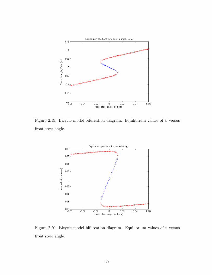
Figure 2.19: Bicycle model bifurcation diagram. Equilibrium values of β versus
front steer angle.
Figure 2.20: Bicycle model bifurcation diagram. Equilibrium values of r versus
front steer angle.
37

2.3 Four-wheel model
Figure 2.21: SAE representation of the 4 wheel model.
The original bicycle model was also extended to a four-wheel model, as a first
step in the development of the vehicle model used in Chapter 3. In the bicycle
model, errors were induced by characterizing the tire forces at each axle based
on average slip angles. In the four-wheel model, individual wheel velocities and
directions were calculated, allowing individual wheel slip angles to be used to
calculate individual tire forces. The tire forces were then applied at the true tire
location, accounting for the full geometry of the vehicle.
The four-wheel case does not share the same symmetry characteristics as the
bicycle model, therefore equivalence did not exist between the SAE standard co-
ordinate system and the coordinates used by Ono. Consequently, the coordinates
were defined according to the SAE standard (Figure 2.21). Two additional vehicle
38
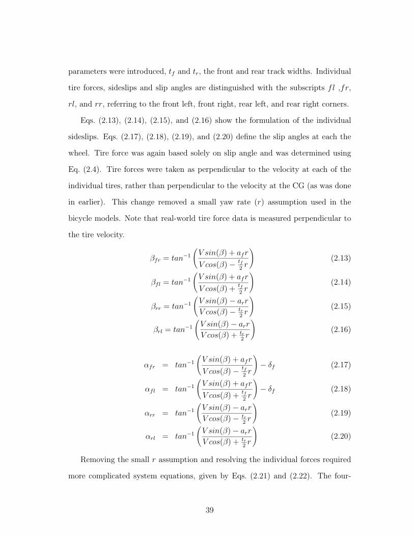
parameters were introduced, tf and tr, the front and rear track widths. Individual
tire forces, sideslips and slip angles are distinguished with the subscripts fl ,fr,
rl, and rr, referring to the front left, front right, rear left, and rear right corners.
Eqs. (2.13), (2.14), (2.15), and (2.16) show the formulation of the individual
sideslips. Eqs. (2.17), (2.18), (2.19), and (2.20) define the slip angles at each the
wheel. Tire force was again based solely on slip angle and was determined using
Eq. (2.4). Tire forces were taken as perpendicular to the velocity at each of the
individual tires, rather than perpendicular to the velocity at the CG (as was done
in earlier). This change removed a small yaw rate (r) assumption used in the
bicycle models. Note that real-world tire force data is measured perpendicular to
the tire velocity.
βfr = tan−1
(V sin(β) + afr
V cos(β)− tf2r
)(2.13)
βfl = tan−1
(V sin(β) + afr
V cos(β) +tf2r
)(2.14)
βrr = tan−1
(V sin(β)− arr
V cos(β)− tr2r
)(2.15)
βrl = tan−1
(V sin(β)− arr
V cos(β) + tr2r
)(2.16)
αfr = tan−1
(V sin(β) + afr
V cos(β)− tf2r
)− δf (2.17)
αfl = tan−1
(V sin(β) + afr
V cos(β) +tf2r
)− δf (2.18)
αrr = tan−1
(V sin(β)− arr
V cos(β)− tr2r
)(2.19)
αrl = tan−1
(V sin(β)− arr
V cos(β) + tr2r
)(2.20)
Removing the small r assumption and resolving the individual forces required
more complicated system equations, given by Eqs. (2.21) and (2.22). The four-
39
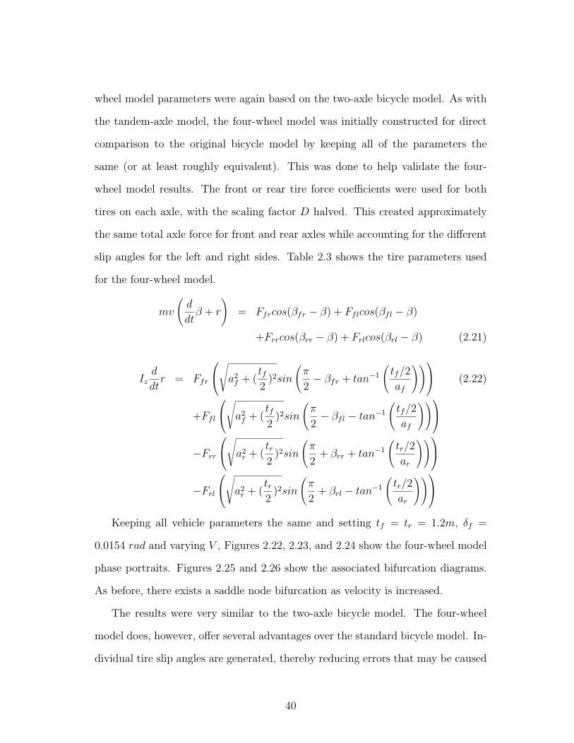
wheel model parameters were again based on the two-axle bicycle model. As with
the tandem-axle model, the four-wheel model was initially constructed for direct
comparison to the original bicycle model by keeping all of the parameters the
same (or at least roughly equivalent). This was done to help validate the four-
wheel model results. The front or rear tire force coefficients were used for both
tires on each axle, with the scaling factor D halved. This created approximately
the same total axle force for front and rear axles while accounting for the different
slip angles for the left and right sides. Table 2.3 shows the tire parameters used
for the four-wheel model.
mv
(d
dtβ + r
)= Ffrcos(βfr − β) + Fflcos(βfl − β)
+Frrcos(βrr − β) + Frlcos(βrl − β) (2.21)
Izd
dtr = Ffr
√a2f + (
tf2
)2sin
(π
2− βfr + tan−1
(tf/2
af
)) (2.22)
+Ffl
√a2f + (
tf2
)2sin
(π
2− βfl − tan−1
(tf/2
af
))−Frr
√a2r + (
tr2
)2sin
(π
2+ βrr + tan−1
(tr/2
ar
))−Frl
√a2r + (
tr2
)2sin
(π
2+ βrl − tan−1
(tr/2
ar
))Keeping all vehicle parameters the same and setting tf = tr = 1.2m, δf =
0.0154 rad and varying V , Figures 2.22, 2.23, and 2.24 show the four-wheel model
phase portraits. Figures 2.25 and 2.26 show the associated bifurcation diagrams.
As before, there exists a saddle node bifurcation as velocity is increased.
The results were very similar to the two-axle bicycle model. The four-wheel
model does, however, offer several advantages over the standard bicycle model. In-
dividual tire slip angles are generated, thereby reducing errors that may be caused
40
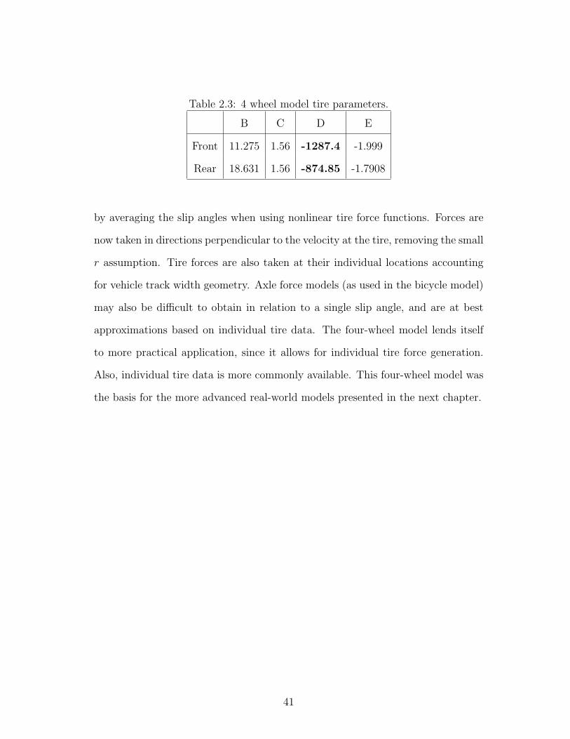
Table 2.3: 4 wheel model tire parameters.
B C D E
Front 11.275 1.56 -1287.4 -1.999
Rear 18.631 1.56 -874.85 -1.7908
by averaging the slip angles when using nonlinear tire force functions. Forces are
now taken in directions perpendicular to the velocity at the tire, removing the small
r assumption. Tire forces are also taken at their individual locations accounting
for vehicle track width geometry. Axle force models (as used in the bicycle model)
may also be difficult to obtain in relation to a single slip angle, and are at best
approximations based on individual tire data. The four-wheel model lends itself
to more practical application, since it allows for individual tire force generation.
Also, individual tire data is more commonly available. This four-wheel model was
the basis for the more advanced real-world models presented in the next chapter.
41

Figure 2.22: Phase portrait for 4 wheel model at V = 10 m/s and δf = 0.015
radians.
Figure 2.23: Phase portrait for 4 wheel model at V = 20 m/s and δf = 0.015
radians.
42
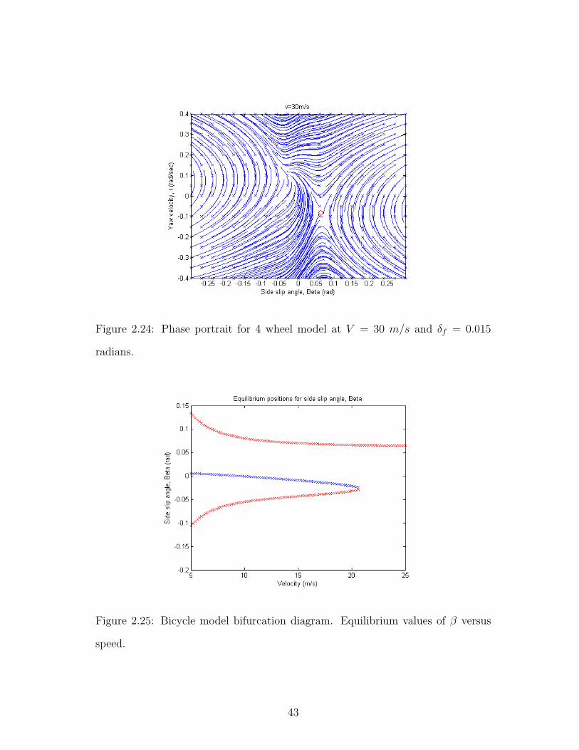
Figure 2.24: Phase portrait for 4 wheel model at V = 30 m/s and δf = 0.015
radians.
Figure 2.25: Bicycle model bifurcation diagram. Equilibrium values of β versus
speed.
43

Figure 2.26: Bicycle model bifurcation diagram. Equilibrium values of r versus
speed.
44
Chapter 3
LTV model
The four-wheeled model introduced in Chapter 2 removed some of the limitations
of the original bicycle model, in that the tire data for the bicycle model needed the
effects of weight transfer and differences in right and left tire slip angles embedded
in the data. In practice, this is not easy to achieve. Because the four-wheel model
uses true tire data (as tested on a tire test rig), the four-wheel model is more easily
and accurately applied to real-world vehicles.
This chapter applies the four-wheel model to a Light-Duty Utility Military
Tactical Vehicle (LTV), and extends the analysis over a broad range of the state
space. The LTV was selected because extensive handling tests of over-weighted
LTVs were recently conducted at the U.S. Army Aberdeen Test Center (ATC),
which provided key vehicle and tire data. It was anticipated that this work might
support and help explain the findings of the testing at ATC. In addition, develop-
ment of an accurate and easily generated math model allows vehicle stability to be
evaluated at all conceivable payload conditions, without the need for extensive and
potentially dangerous field tests at the limits of performance. Lastly, a four-wheel
model with lateral weight transfer is presented and briefly discussed.
45

3.1 Tire Model
The first step in creating a vehicle model is developing a realistic tire model. The
tire model used by Ono et al. [18] was a very general form of a semi-empirical
tire model commonly refereed to as “The Magic Tire Formula”. A more advanced
version of this formulation was used in the current LTV model. The new formula-
tion allowed tire force to be characterized by both slip angle and vertical load (as
opposed to slip angle alone) from a limited set of tire data obtained under specific
loading conditions. The improved tire model also allowed for the creation of more
complicated vehicle models that included roll motions and dynamic lateral loading
conditions of the tires.
The following sections of the paper present the general formulation of the Magic
Tire formula, a genetic algorithm for coefficient optimization, and a means to over-
come shortfalls in the range of the available test data. More specifically, guidelines
are presented to extend tire data limited below saturation to regions beyond sat-
uration.
3.1.1 The Magic Tire Formula
The initial tire model considered for the LTV model used the full version of the
magic tire formula [19]. This semi-empirical formula is regarded as the foremost
tire force model for vehicle dynamic simulations to date [20], and has been shown to
very accurately represent tire data [13] [3] [19]. The model used for this simulation
was a pure slip model for tire lateral force, whereby tire lateral force was defined
as a function of normal load and slip angle. Camber and combined longitudinal
and lateral slip effects were neglected.
The Magic Tire Formula is re-written in general terms in Eq. (3.1), where X can
46

represent either longitudinal slip ratio or lateral slip angle, and Y represents the
corresponding longitudinal or lateral forces. An additional offset term, Eq. (3.2)
can also be included. The Magic Tire Formula produces the classic “S-shaped tire
curves as shown in Figure 3.1.
y(x) = D · sin[C · tan−1
{B · x− E ·
(B · x− tan−1(B · x)
)}](3.1)
Ypure(X) = y(x) + Sv
x = X + Sh (3.2)
Figure 3.1: General Magic Tire Formula slip curve [19].
The coefficients B, C, D, E, Sh, and Sv are curve fitted parameters that
describe the relationship between lateral force and slip angle at a given vertical
load. Physically, D represents the maximum slip value, B · C · D represents the
47

cornering stiffness at low slip angles (slope of the curve near the origin), and
Sh and Sv represent offsets due to non-symmetric effects such as ply steer and
conicity. C and E are shape factors that do not have obvious physical meaning.
Mathematically, C defines the region of influence of the sin function, while E
influences the curvature at the peak value [19].
Eq. (3.1) gives force solely as a function of the slip angle. Since tire lateral force
is a function of both slip angle and vertical load, Eqs. (3.3) through (3.9) were used
to account for vertical load (without camber effects). In the full formulation, the
general coefficients, B, C, D, Sh, and Sv, are functions of vertical load, and E is a
function of both vertical load and slip angle. There are now 12 coefficients, a0, a1,
a2, a3, a4, a6, a7, a8, a9, a11, a12, and a17. These are curve-fitted parameters that
capture the relationship of the general coefficients to vertical load. In the complete
formulation, tire slip angle and vertical load were used in Eqs. (3.3) through (3.9)
with the curve-fitted parameters,a0, a1, a2, a3, a4, a6, a7, a8, a9, a11, a12, and a17,
to generate values for the general coefficients, B, C, D, E, Sh, and Sv. The values
for the general coefficients were then used in Eqs. (3.1) and (3.2), with the slip
angle, to calculate a lateral tire force.
D = a1 · F 2z + a2 · Fz (3.3)
C = a0 (3.4)
B · C ·D = a3 · sin(2 · tan−1(
Fz
a4
))
(3.5)
B = (B · C ·D)/(C ·D) (3.6)
E = (a6 · Fz + a7) · (1− a17 ∗ sgn(α + Sh)) (3.7)
Sh = a8 · Fz + a9 (3.8)
Sv = a11 · Fz + a12 (3.9)
48
3.1.2 The genetic optimization algorithm
The 12 magic tire coefficients were fit to empirical tire data. The curve fit was
a multi-parameter, single-objective, unconstrained optimization procedure. The
optimization procedure converges upon parameter values that minimize the sum
of the squared errors between the magic tire formula values and the tire data. A
genetic optimization algorithm, developed in [3], was used. This procedure was
found to produce accurate results without the need for precise initial guesses, while
converging reasonably fast.
Genetic algorithms (GAs) are based on the principle of evolution. A basic
GA starts with a set of randomly generated possible solutions. Each possible
solution is treated as an individual in a population (the set). The population then
goes through a series of selection, reproduction, and mutation processes, with the
general tendency toward individuals with preferred solutions. Preferred solutions
are solutions that are superior in terms of the objective function. In this case,
preferred solutions are solutions that have lower mean squared errors.
Other algorithms considered for use involved items such as sub-populations
that evolve somewhat independently, where limited inter-population contact is
allowed [14]. These algorithms increase complexity and overall computation time.
The more complicated algorithms were tested but did not consistently produce
accurate results for this problem.
The curve fit is a multi-parameter optimization, since all 12 coefficients must be
optimized for the single objective function. In the GA, each individual is comprised
of a single possible solution to the optimization. Therefore, each individual is
defined by only 12 values, or genes, one for each of the parameters.
In the algorithm used, each iteration begins with the selection of the best indi-
49

vidual from the entire population. The algorithm then processes each individual in
the population. For each individual, two individuals from the population are ran-
domly selected (population sample) and combined to create a perturbing vector.
This perturbation is added to the best individual forming a reproduction candi-
date. Each individual may have a different reproduction candidate, since each has
a different perturbation vector (created from a different population sample). The
individual is then potentially crossed (mated) with the reproduction candidate.
If crossing occurs, there is a potential for mutations in the genes being passed.
The product of the crossing (the child) can then be used to form the subsequent
generation.
The entire population is made up of NP individuals. Each individual can be
represented as Xi where i ∈ [1, NP ]. Each individual Xi, consists of a 12 element
vector. Xi,j : j ∈ [1, 12] represents the jth gene or coefficient of the possible
solution Xi.
During each iteration, Xbest represents the best solution in the population. For
each individual a sample of two individuals from the population is selected (Xr1
and Xr2 ). The reproduction candidate is then created by Eq. (3.10). F is a real
valued parameter and represents the amount of perturbation applied to Xbest.
V = Xbest + F · (Xr1 −Xr2) (3.10)
Each individual is then potentially crossed with their reproduction candidate.
Crossing (mating) occurs with a probability of CP . If crossing occurs, genes are
randomly selected (with equal probability) from each parent to form the child.
The child is then compared to the original individual. If the child is a preferred
solution, the individual is replaced.
If crossing occurs, there is also a possibility of mutation as the genes are passed
50

from parent to child. MP represents the mutation probability of each gene. For
a rapidly converging solution, MP is often chosen to be much less than CP ([3]).
When mutation occurs, the gene that is passed is adjusted within a range propor-
tional to the value of the gene. If gene y is passed, and mutation is occurring,
Eq. (3.11) represents the equation for the mutated gene, ym. MR is a real-valued
parameter that adjusts the mutation range. The lower the value of MR, the larger
the allowed mutation range (compared to the value of the original gene). The ex-
pression rand(i, j) represents a random number generated from a uniform random
distribution function between values i and j.
ym = y + rand(−y/MR, y/MR) (3.11)
Iterations run until the best individual (solution) converges within an ac-
ceptable error, the solution does not change within several iterations (algorithm
stalled), or the maximum number of iterations is exceeded. For this curve fit, the
acceptable error was set very low to allow the algorithm to fully converge. Also, F ,
CP , MP , and MR were chosen to keep the algorithm from stalling away from the
optimal solution. Computational time was not of great significance. So, the run
termination was mainly based on the maximum number of iterations. A flowchart
depicting the algorithm is shown in Figure 3.2.
51

Figure 3.2: GA flowchart.
52
3.1.3 Results of the algorithm
The algorithm was first tested using data found in the literature [3]. The GA was
run with the following parameters: NP = 50, CP = 0.6, MP = 0.1, F = 0.4,
MR = 4, and itermax = 1000. Figure 3.3 shows the mean square error of the
best individual of the population vs. the number of iterations. Figure 3.4 shows
the results from the output of the algorithm versus the actual data. Actual data
points are represented in this Figure by the x’s, and algorithm results are plotted
as solid lines. The algorithm was trained on the lowest and the highest vertical
loads. Results for the middle loading condition showed good match to the actual
data, demonstrating the accuracy of the formulation as well as the optimization
algorithm. The algorithm periodically failed to converge fully. But aside from the
obvious qualitatively bad fits, the results were consistent and repeatable in terms
of the values of the formula output (often the coefficients would not be exactly the
same but formula outputs were consistent).
53

Figure 3.3: Genetic algorithm mean square error vs. iterations.
Figure 3.4: Tire force vs. slip angle, GA results.
54

3.1.4 Modified formulation
In practice, tire data at high slip (peak and past saturation) is not always taken.
In addition to being destructive to the tires, excessive wear and inconsistent tem-
peratures make the high slip data less repeatable [22] [21] [20] . Near the friction
limit of the tire, forces also become dependent on speed as well as temperature,
again leading to unrepeatable data [21] [20]. Nevertheless, lack of high-slip data
can lead to unpredictable model behavior at the higher slip angles.
The LTV tire data obtained for this research suffered from this shortfall, in
that it generally did not include results up to or beyond tire saturation. Figures
3.5, 3.6 and 3.7 are plots of measured values for lateral tire forces vs. slip angle at
several vertical loads, while the actual values are given in Tables 3.1.4, 3.1.4 and
3.1.4. This section describes the approach developed to overcome this shortfall.
Initially all of the curve fits were run with the following parameters: NP = 50,
CP = 0.6, MP = 0.1, F = 0.4, MR = 3, and itermax = 1000. The parameters
were chosen to provide quick convergence and few occurrences of stalling at poor
fit local minimums. The early algorithm produced fairly consistent and well fitting
results (low square errors). However, repeatability of lateral force values at higher
slip angles (past the slip angle span of the data) was poor. This was attributed to
the tradeoff between the parameters C and E, called the shape factors.
For data with limited slip ranges, one shape factor can be traded for the other
without affecting fitment of the unsaturated data [21]. Accordingly, C values can
be fixed without effecting fitment to the data [21] [23]. Sharp showed when high
lateral slip data is unavailable, the creation of a normalized combined slip curve
(taking into account both longitudinal and lateral slip) can be eased by setting
the C value for lateral force to the value optimized for longitudinal slip [21]. In
55
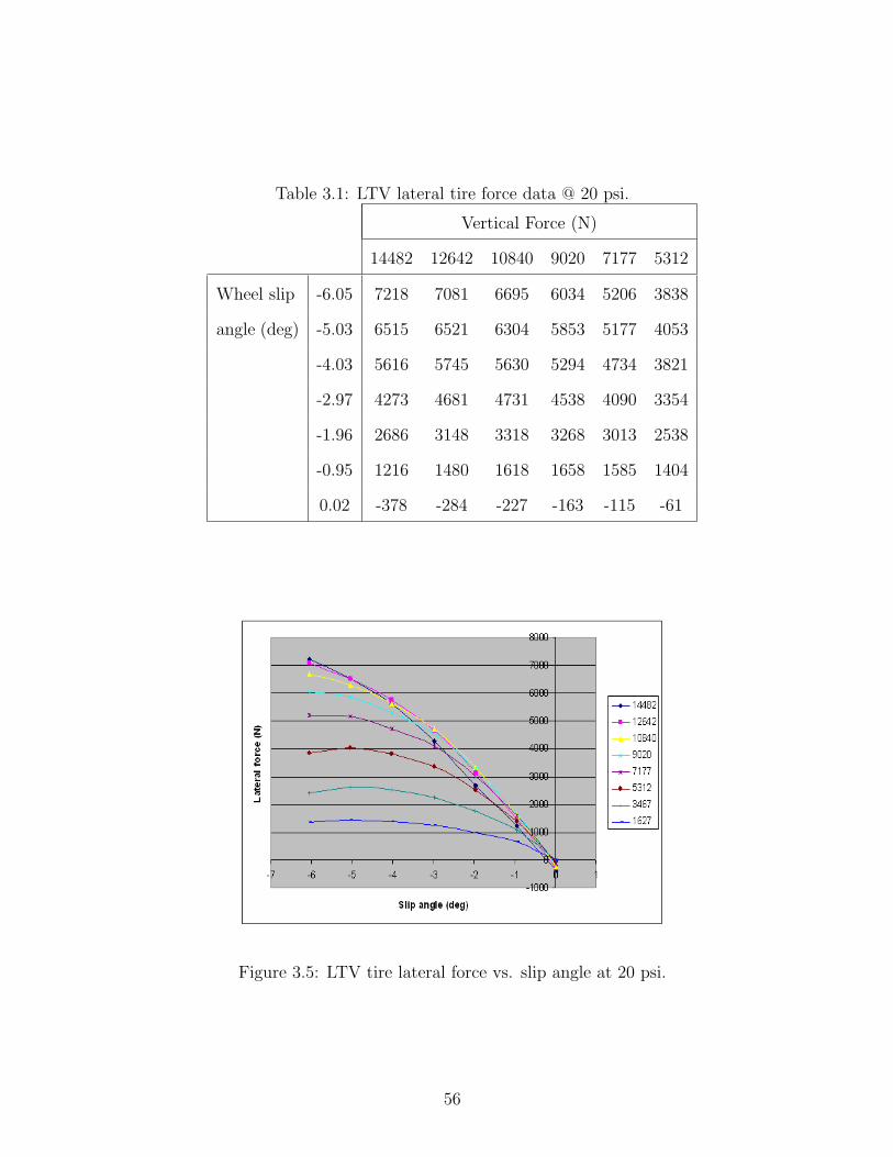
Table 3.1: LTV lateral tire force data @ 20 psi.
Vertical Force (N)
14482 12642 10840 9020 7177 5312
Wheel slip -6.05 7218 7081 6695 6034 5206 3838
angle (deg) -5.03 6515 6521 6304 5853 5177 4053
-4.03 5616 5745 5630 5294 4734 3821
-2.97 4273 4681 4731 4538 4090 3354
-1.96 2686 3148 3318 3268 3013 2538
-0.95 1216 1480 1618 1658 1585 1404
0.02 -378 -284 -227 -163 -115 -61
Figure 3.5: LTV tire lateral force vs. slip angle at 20 psi.
56

Table 3.2: LTV lateral tire force data @ 35 psi.
Vertical Force (N)
21805 19055 16335 13605 10899 8164 5434 2750
Wheel slip -6.05 9488 9688 9360 8713 7743 6187 3978 1997
angle (deg) -5.03 8434 8801 8673 8182 7355 5985 3978 1965
-4.03 7159 7607 7593 7244 6548 5397 3671 1809
-2.97 5501 6085 6190 5979 5449 4531 3131 1544
-1.96 3654 4140 4299 4199 3875 3268 2325 1170
-0.95 1518 1817 1972 1982 1874 1634 1226 696
0.02 -673 -623 -542 -466 -399 -294 -185 -61
Figure 3.6: LTV tire lateral force vs. slip angle at 35 psi.
57

Table 3.3: LTV lateral tire force data @ 50psi.
Vertical Force (N)
27744 24263 20809 17345 13861 10406 6966 3503
Wheel slip -6.05 11853 11926 11497 10674 9393 7452 4846 2357
angle (deg) -5.03 10625 10900 10643 9966 8821 7100 4751 2292
-4.03 9217 9488 9329 8762 7793 6353 4300 2108
-2.97 7217 7574 7535 7145 6409 5270 3608 1778
-1.96 4859 5217 5273 5048 4549 3764 2640 1319
-0.95 2050 2305 2418 2387 2191 1873 1397 748
0.02 -803 -717 -619 -541 -450 -324 -197 -50
Figure 3.7: LTV tire lateral force vs. slip angle at 50 psi.
58
this case, since there was no saturation slip data available, a general shape was
assumed. In order to provide more consistent results, a typical lateral slip C value
of 1.30 was chosen [22].
Figure 3.8 shows the initial algorithm results for lateral force at the highest
vertical load and relatively high slip angle (past saturation) for each tire pressure.
Figure 3.9 shows the results after holding C = 1.3. Both are plotted against the
sum of the mean square errors so that the values can be compared against their
quality of fit. The y axes are scaled the same to allow direct comparison. The
majority of the solutions fell within the [0, 10] kN2 range for the mean square
error. Solutions having a sum square error of less than 10 kN2 for 56 points
(roughly 13N error per point) can be said to have very good fits. Both cases show
a good clustering of data in terms of fit quality (the majority had very good fit).
However, holding C = 1.3, only provided marginally better clustering in the high
slip values showing marginally better repeatability.
The major issue with the curve fit was that the test data showed some unex-
pected results for the highest load at each of the tire pressures. Lateral force data
were, for some slip angles, lower than those for the lower vertical load conditions.
This can be seen in Figures 3.5, 3.6 and 3.7. Figures 3.10 and 3.11 show typical
qualitatively poor solutions converged upon by the GA. Fitment to the data was,
however, good in both examples. In the full magic tire formulation, E was allowed
to change with vertical load. The poor solutions were attributed to the change in
E, in order to better fit the data for the highest load condition. Figures 3.12 and
3.13 show the sharp drop in lateral force at the corresponding value for the highest
load. Again, this was due to the algorithm attempting to match the unexpected
data.
59
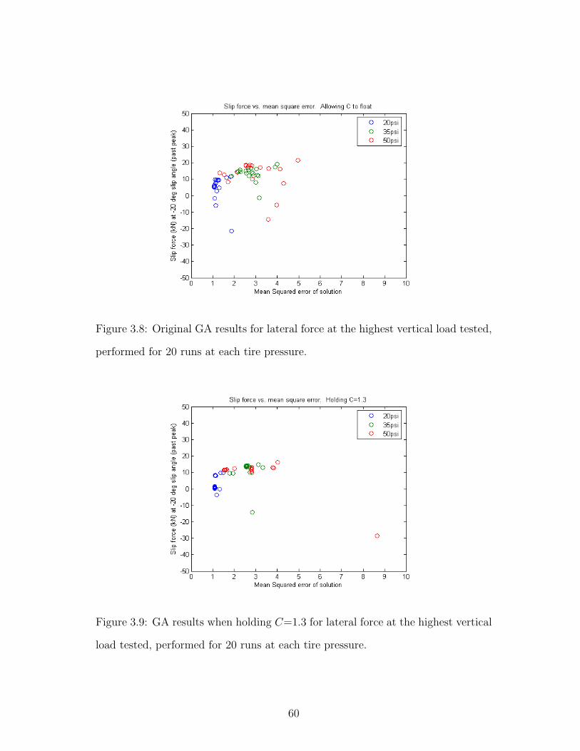
Figure 3.8: Original GA results for lateral force at the highest vertical load tested,
performed for 20 runs at each tire pressure.
Figure 3.9: GA results when holding C=1.3 for lateral force at the highest vertical
load tested, performed for 20 runs at each tire pressure.
60

Figure 3.10: Example of undesirable GA solution for 35 psi, C=1.3, E allowed to
float according to full tire model formulation.
Figure 3.11: Example of undesirable GA solution for 50 psi, C=1.3, E allowed to
float according to full tire model formulation.
61

Figure 3.12: Lateral force vs. vertical load for undesirable solution at 35 psi.
Figure 3.13: Lateral force vs. vertical load for undesirable solution at 50 psi.
62
If E was allowed to vary with the algorithm, but held as a constant with
respect to vertical load and slip angle (in contrast to the magic tire formulation),
the shape characteristics were more consistent at the higher slips for all of the
loads. A constant E value is used in many formulations of the magic tire formula
[22] [23] [21] [20]. In fact, for the normalization procedure for combined slip, the
E was not only constant but was set at a certain value determined by the solution
of the pure slip cases [22] [23] [21] [20].
Figures 3.14 and 3.15 show the results of the algorithm where C = 1.3 and
E was constrained to be a constant. Since E was not allowed to vary with load,
the shape of the highest load curve was forced to resemble that of the lower load
curves. This led to a slightly poorer fit, but more consistent and repeatable results.
With a mean squared error of about 4 kN for the 56 points, the fit was still very
good. This method was used with similar results for all of the tire pressures. All
of the curves generated for the LTV tire model were generated in this fashion.
Figures 3.16 and 3.17 show the curve fits for the data using the modified strat-
egy of setting C = 1.3 and constraining E as a constant. Table 3.1.4 summarizes
the results of the algorithm for the LTV tire data. The parameter E was optimized
as a constant, and no longer followed the full formulation as defined in Eq. (3.3).
Instead, E was simply defined as E = a6. In this case a7 and a17 were dummy
variables that were not optimizable and did not effect the solution.
63

Figure 3.14: Example of a desirable GA solution for 50 psi, C=1.3, E=optmized
constant.
Figure 3.15: Lateral force vs. vertical load for desirable solution at 50 psi.
64

Figure 3.16: Lateral force vs. slip angle for 20 psi data.
Figure 3.17: Lateral force vs. slip angle for 35 psi data.
65

Table 3.4: LTV GA coefficient results.
20 psi 35 psi 50 psi
MSE 1.1087 3.2904 4.3422
a0 1.3000 1.3000 1.3000
a1 -0.0166 -0.0115 -0.0116
a2 0.8315 0.8447 0.8460
a3 97.7925 -123.6505 -152.1290
a4 -8.9904 14.2730 22.0333
a6 -1.2362 -0.8073 -1.0117
a7 3.2413 0.0272 0.3653
a8 0.0000 0.0000 0.0000
a9 -0.0000 -0.0000 -0.0000
a11 0.0000 0.0000 0.0000
a12 -0.0000 0.0000 -0.0001
a17 0.1213 0.0594 -3.2834
66

3.2 LTV four-wheel model results
A heavily loaded LTV was modelled with the following vehicle parameters: af =
1.8059m, ar = 1.4961m, Iz = 6237kg ·m2, m = 3182kg, and tf = tr = 1.7907m.
Front steer was set to a constant, δf = 0.015rad. The tire model was run with
35 psi pressure up front, and 50 psi in the rear. Tire pressures were selected
according to the manufacturers recommendations based on the static wheel loading
conditions. In this initial model, lateral weight transfer was neglected, so the
vertical wheel loads were held constant. As such, tire forces were dependent on the
individual tire parameters and slip angle alone, just as with the earlier theoretical
model.
The LTV vehicle configuration was similar to the theoretical models in that
the normalized rear tire forces were generally less than that of the fronts. Figures
3.18, 3.19, and 3.20 show the phase portraits for the LTV model as velocity was
increased. Again a saddle node bifurcation is evident.
In this model a symbolic expression of the Jacobian matrix of the state equa-
tions was created. Solving for the eigenvalues of the Jacobian at each equilibrium
point allowed for a quantitative characterization of the stability at each point. In
these phase plots, the saddle points are marked by a red diamond while the stable
point is marked with a red square.
As expected, the real parts of the saddle point eigenvalues were positive and
negative. This meant that along certain directions each saddle point was attractive
(stable) and along other directions the point was repulsive (unstable). The eigen-
vectors correspond to the local (linearized) stable and unstable directions. Per-
turbing the equilibrium point slightly in the direction of the eigenvector associated
with the unstable eigenvalue, and integrating forward through time, produced the
67

trajectory along which the saddle point is repulsive. These are trajectories that are
directly leaving the saddle point. Perturbing slightly in the direction of the eigen-
vector associated with the stable eigenvalue, and integrating backward through
time produced the trajectory on which the saddle point is attractive. These cor-
respond to trajectories that travel into the saddle point. Trajectories that go into
and out of the saddle point are called homoclinic orbits. The homoclinic orbits
are plotted on the phase portraits in green. The dotted lines are the orbits head-
ing toward the saddle point and the solid lines are moving away from the point.
These orbits are interesting because the plots are full phase portraits of a time in-
variant system. None of the trajectories cross, so the homoclinic orbits define the
stable manifold (domain of attraction) of the stable focus (in the pre-bifurcation
portraits).
Figures 4.9 and 4.10 are the bifurcation diagrams for the system. Again, a
saddle node bifurcation was evident.
3.3 Expanded model
So far, the phase portraits have been viewed within a window of practical stability
limits. Any trajectory that travels outside of the window may in a practical sense
be considered unstable. However, additional insight into system stability can be
gained by expanding the window and allowing for a full cycle of β. To accomplish
this, all small angle assumptions had to be removed. Although the four-wheel
system equations made no such assumptions, the tire model assumed small slip
angles. Consequently, changes to the tire force model were required.
68

Figure 3.18: Phase portrait for LTV 4 wheel model at V = 10 m/s and δf = 0.015
radians.
Figure 3.19: Phase portrait for LTV 4 wheel model at V = 27 m/s and δf = 0.015
radians.
69

Figure 3.20: Phase portrait for LTV 4 wheel model at V = 36 m/s and δf = 0.015
radians.
Figure 3.21: Bifurcation diagram for LTV 4 wheel model, equilibrium values of β
versus speed.
70
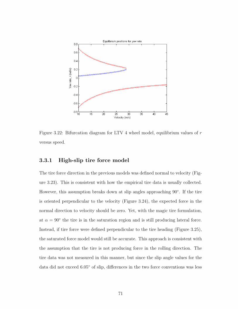
Figure 3.22: Bifurcation diagram for LTV 4 wheel model, equilibrium values of r
versus speed.
3.3.1 High-slip tire force model
The tire force direction in the previous models was defined normal to velocity (Fig-
ure 3.23). This is consistent with how the empirical tire data is usually collected.
However, this assumption breaks down at slip angles approaching 90◦. If the tire
is oriented perpendicular to the velocity (Figure 3.24), the expected force in the
normal direction to velocity should be zero. Yet, with the magic tire formulation,
at α = 90◦ the tire is in the saturation region and is still producing lateral force.
Instead, if tire force were defined perpendicular to the tire heading (Figure 3.25),
the saturated force model would still be accurate. This approach is consistent with
the assumption that the tire is not producing force in the rolling direction. The
tire data was not measured in this manner, but since the slip angle values for the
data did not exceed 6.05◦ of slip, differences in the two force conventions was less
71
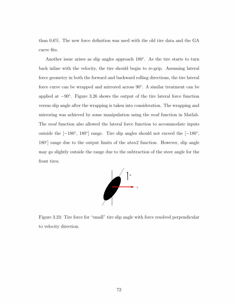
than 0.6%. The new force definition was used with the old tire data and the GA
curve fits.
Another issue arises as slip angles approach 180◦. As the tire starts to turn
back inline with the velocity, the tire should begin to re-grip. Assuming lateral
force geometry in both the forward and backward rolling directions, the tire lateral
force curve can be wrapped and mirrored across 90◦. A similar treatment can be
applied at −90◦. Figure 3.26 shows the output of the tire lateral force function
versus slip angle after the wrapping is taken into consideration. The wrapping and
mirroring was achieved by some manipulation using the mod function in Matlab.
The mod function also allowed the lateral force function to accommodate inputs
outside the [−180◦, 180◦] range. Tire slip angles should not exceed the [−180◦,
180◦] range due to the output limits of the atan2 function. However, slip angle
may go slightly outside the range due to the subtraction of the steer angle for the
front tires.
Figure 3.23: Tire force for “small” tire slip angle with force resolved perpendicular
to velocity direction.
72

Figure 3.24: Tire force direction for 90◦ tire slip angle with force resolved perpen-
dicular to velocity direction.
Figure 3.25: Tire force direction for 90◦ tire slip angle with force resolved perpen-
dicular to tire heading.
Figure 3.26: Wrapped tire lateral force function.
73
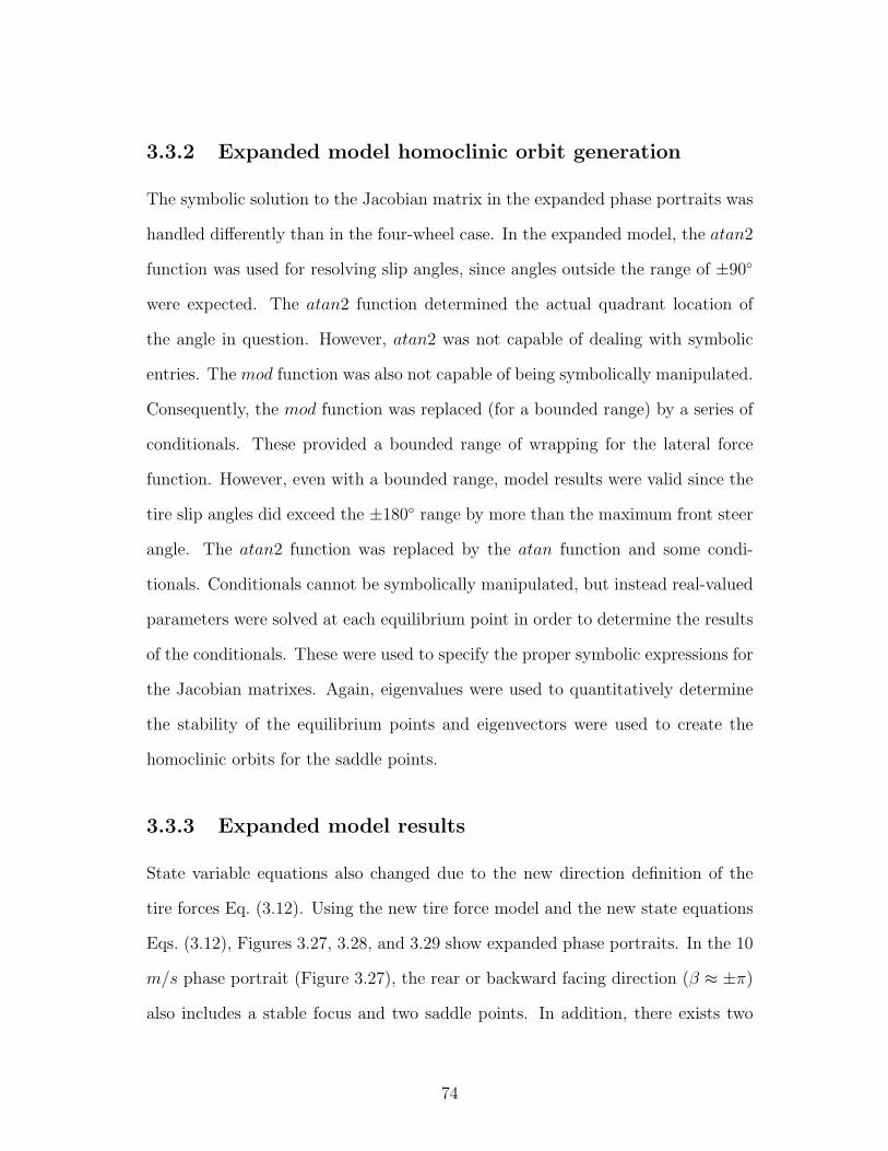
3.3.2 Expanded model homoclinic orbit generation
The symbolic solution to the Jacobian matrix in the expanded phase portraits was
handled differently than in the four-wheel case. In the expanded model, the atan2
function was used for resolving slip angles, since angles outside the range of ±90◦
were expected. The atan2 function determined the actual quadrant location of
the angle in question. However, atan2 was not capable of dealing with symbolic
entries. The mod function was also not capable of being symbolically manipulated.
Consequently, the mod function was replaced (for a bounded range) by a series of
conditionals. These provided a bounded range of wrapping for the lateral force
function. However, even with a bounded range, model results were valid since the
tire slip angles did exceed the ±180◦ range by more than the maximum front steer
angle. The atan2 function was replaced by the atan function and some condi-
tionals. Conditionals cannot be symbolically manipulated, but instead real-valued
parameters were solved at each equilibrium point in order to determine the results
of the conditionals. These were used to specify the proper symbolic expressions for
the Jacobian matrixes. Again, eigenvalues were used to quantitatively determine
the stability of the equilibrium points and eigenvectors were used to create the
homoclinic orbits for the saddle points.
3.3.3 Expanded model results
State variable equations also changed due to the new direction definition of the
tire forces Eq. (3.12). Using the new tire force model and the new state equations
Eqs. (3.12), Figures 3.27, 3.28, and 3.29 show expanded phase portraits. In the 10
m/s phase portrait (Figure 3.27), the rear or backward facing direction (β ≈ ±π)
also includes a stable focus and two saddle points. In addition, there exists two
74

unstable foci marked in the diagram by a red star. As velocity is increased to
27 m/s (pre-bifurcation in the forward facing direction), the saddle points and
stable foci in the rear facing direction disappeared. This demonstrated bifurcations
occurring in the rear facing directions at a point prior to the one occurring in the
forward direction (with respect to velocity). As velocity was increased to 36 m/s
(post-bifurcation in the forward direction) the stable focus still existed in the rear. β
r
=
Ffr·cos(β−δf )+Ffl·cos(β−δf )+Frr·cos(β)+Frl·cos(β)
mv− r
(Ffr+Ffl)cos(δf )af+(Ffr−Ffl)sin(δf )tf2−(Frr+Frl)ar
Iz
(3.12)
Figure 3.27: Expanded phase portrait for LTV 4 wheel model at V = 10 m/s and
δf = 0.015 radians.
75

Figure 3.28: Expanded phase portrait for LTV 4 wheel model at V = 27 m/s and
δf = 0.015 radians.
76
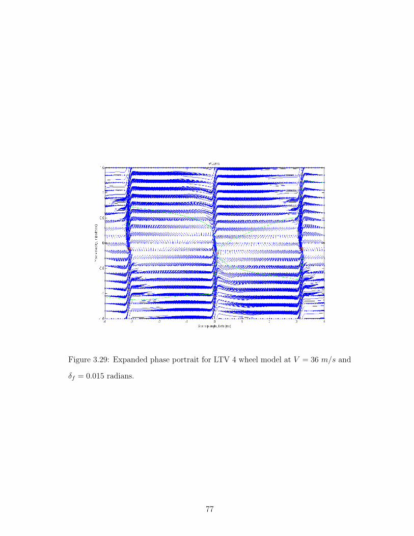
Figure 3.29: Expanded phase portrait for LTV 4 wheel model at V = 36 m/s and
δf = 0.015 radians.
77

3.4 Lateral load transfer model
So far, lateral weight transfer and roll dynamics have not been considered. A final
model was developed to include their effects. In doing so, additional states were
introduced in the system.
3.4.1 Additional states
The lateral force model included six additional states. Two were for roll angle
and roll rate, and four were for each of the tire forces. In order to describe the
propagation of these new states, a detailed look at the vehicle roll dynamics was
required.
Figure 3.30: Vehicle roll axis.
The variable ε is defined as the inclination angle of the roll axis, illustrated
in Figure 3.30, and can be described using Eq. (3.13). The terms hf and hr are
the roll center heights at the front and rear axles, respectively. The roll axis is
assumed to lie in the vehicle x-z plane. The term h1 is the height of the CG above
the roll axis.
ε = tan−1(hf − hr)/L (3.13)
78

Figure 3.31 shows the free body diagram for the unsprung mass at either axle.
The system is in static equilibrium. Inertial forces from the body are treated as
reactive forces through the theoretical pinned joint at the roll axis. Fy and Fz are
the tire lateral and normal forces. The term φ is the roll angle of the body and
the moments are the reaction moments due to the roll stiffness and roll damping
of the vehicle.
Figure 3.31: Unsprung mass free body diagram.
Figure 3.32 is the free body diagram of the sprung mass viewed as a longitudinal
section at the center of gravity. Forces from the unsprung mass system are acted
through the pinned joint at the roll axis, and reacted by inertial forces at the
center of gravity. The term m is the vehicle sprung mass. Eq. (3.14) was obtained
by balancing the forces in both free body diagrams. Roll stiffness (kφ) and roll
damping (cφ) for the sprung mass equate to the sum of the front and rear roll
stiffnesses and roll damping rates, Eq. (3.15). The reaction moments are shown in
Eq. (3.16).
Fz = mg
79

Fy = may = Fyfl + Fyfr + Fyrl + Fyrr (3.14)
kφ = kφf + kφr
cφ = cφf + cφr (3.15)
Mkφ= kφφ
Mcφ= cφφ (3.16)
Figure 3.32: Sprung mass free body diagram.
Resolving moments about the roll axis location at the CG (Figure 3.32) yields
Eq. (3.17), where Iφ is the full body roll moment of inertial. Equation (3.17)
describes the propagation of the roll angle through time given the lateral tire forces.
For the unsprung mass, it was assumed that rotational velocity and acceleration
effects were negligible (low roll inertia of unsprung mass and wheels remain planted
on the ground). Therefore, moments due to tire forces balanced the moment
created by the roll stiffness and damping terms, Eqs. (3.18) and (3.19). With these
equations, vertical load on each tire can be calculated when tire lateral forces, roll
80

angle and roll rate are known.
Iφφ = −kφφ− cφφ + [mg · h1 · sin φ + Fyh1 cos φ] · cos ε (3.17)
The previous models assumed the tires would instantaneously produce their
steady-state tire force output. In this case, lateral force is required to determine
vertical load, which is in turn required in the tire model to determine lateral force.
Therefore, a tire force propagation model was used. Eq. (3.20) depicts the tire lag
model, which propagated the tire side force at each time step. The tire lag model
was used to calculate transient tire forces from steady-state tire force values. Fy is
the steady-state tire force value and was determined using the magic tire formula,
with the vertical load and slip angle as inputs. The term σ is the lag coefficient of
the tire.
In terms of the numerical integration, at each time increment tire vertical load
was determined using the roll angle, roll rate and the tire lateral force states
Eqs. (3.18) and (3.19). Individual tire slip angles were calculated from β and r in
the same manner as the four-wheel model. The vertical load combined with the
individual tire slip angles was used to calculate Fy from the magic tire formula. Fy
then determined the propagation of the lateral tire forces, Eq. (3.20). Roll angle
and roll rate states were propagated using tire lateral force Eq. (3.17). The states
β and r were propagated using the same method as the non-lateral load model,
except that tire forces were no longer directly calculated. They are provided by
the tire force states.
0 = −kφfφ− cφf φ + [tf2
(Fzfl − Fzfr)− hf (Fyfr + Fyfr)] cos ε (3.18)
0 = −kφrφ− cφrφ + [tr2
(Fzrl − Fzrr)− hr(Fyrr + Fyrr)] cos ε (3.19)
81

Fy =v
σ(Fy − Fy) (3.20)
3.5 Lateral load model results
For the phase portraits, roll angle, roll rate and all of the tire lateral forces were
initially set to zero. This corresponded to a situation where the vehicle was initially
translating and yawing at a rate corresponding to the initial values for β and r,
but the tires are not making contact with the road. At time t = 0, the tires make
contact and tire lateral force and body roll dynamics begin. This led to very busy
phase portraits since each trajectory had to initially build up tire forces and roll
angle.
To remove some of the “transient” dynamics in the additional states, better
initial conditions were generated. Since each starting point was only defined in the
β and r plane, the “steady state” values at each starting point were approximated
for the additional states. Initial tire lateral forces were approximated by the steady-
state value of the tire forces at the static loading condition and the initial slip angles
given by the initial values for β and r. Roll angle was approximated by the initial
tire lateral force values, and roll rate was set to zero. This simplified some of the
“transient” responses as the simulation first began.
Figures 3.33, 3.34, and 3.35 are the phase portraits for the lateral load transfer
model, using the same vehicle parameters and tire pressures as before. Because the
β-r plane is only a projection in the full 8-degree-of-freedom (DOF) state space,
the trajectories cross.
Equilibrium points were then calculated by setting the rate of change to zero
for all the states (including the six new states). This corresponded to a situation
where the body no longer rolled and the tires reached steady-state force (in addition
82

to the equilibrium conditions for β and r). Homoclinic orbits were not created
in this case. The orbits would only represent a projection onto the β-r plane.
The determination of the domain of attraction for the stable points can only be
represented in the full state space. This can also be understood by observing the
crossing of the trajectories. Since trajectories cross in the projected plane, the
projected homoclinic orbits do no define regions of attraction.
Figure 3.33: Phase portrait for lateral load transfer model at V = 10 m/s and
δf = 0.015 radians.
83

Figure 3.34: Phase portrait for lateral load transfer model at V = 25 m/s and
δf = 0.015 radians.
84
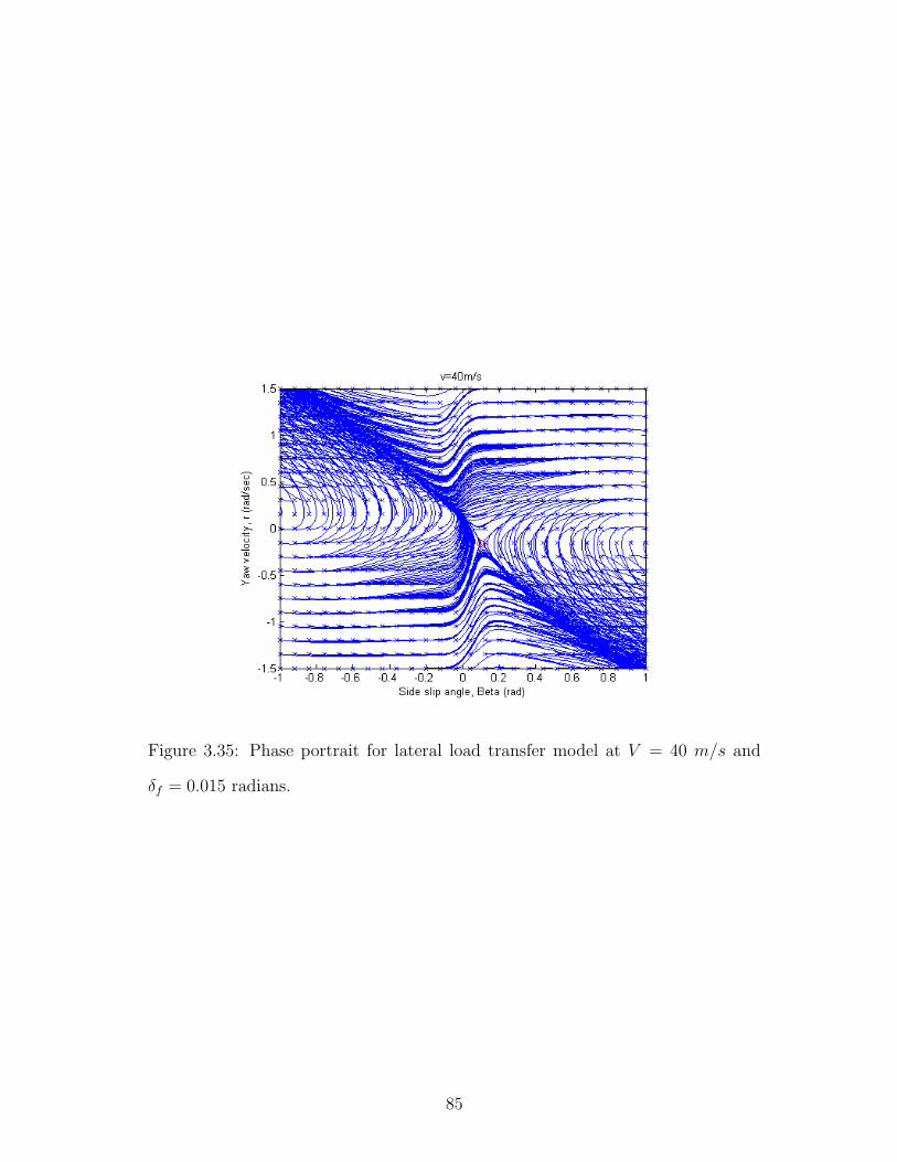
Figure 3.35: Phase portrait for lateral load transfer model at V = 40 m/s and
δf = 0.015 radians.
85

Chapter 4
Analysis and observations
This chapter discusses the links between the analytical model and physical vehicle
maneuvering. Interpretations of phase portraits are presented including physical
meanings of equilibrium (steady-state) solutions. Bifurcation diagrams are exam-
ined and compared to vehicle handling tests. Analytic and physical stability dif-
ferences are presented and some model limitations are discussed for the expanded
model. US/OS/NS are discussed with respect to the nonlinear tire models, and
bifurcation examples are presented for understeering and neutral steering vehicles.
Finally, the lateral load model and its results are examined.
4.1 Phase portraits
Phase portraits provide a unique way to identify system behavior over a broad set
of vehicle operating conditions. Their most basic interpretation relates to steady-
state or quasi-steady-state behavior, though they can provide some insight into
transient behavior as well. First, application to steady-state and quasi-steady-
state conditions will be discussed by relating the portraits to the so-called slow
input steer test.
86

Field tests often begin at some constant velocity and zero steer angle, meaning
zero sideslip and zero yaw rate. This corresponds to the stable equilibrium con-
dition for zero steer angle in the phase portraits. Steer angle is slowly increased
(slow enough to make keep roll and yaw rate very small) until some limit in per-
formance is reached. If steer angle were increased in small discrete steps (as is
done in constant radius tests with velocity), the resulting dynamics would resem-
ble the phase portraits at each step. Note that the steady-state field test only
captures the equilibrium state at each condition. The phase portraits offer much
more information.
The initial vehicle state after a step is made falls within the domain of attraction
of the stable solution under the new vehicle conditions. The vehicle moves to the
new stable solution, as shown by the vectors in the phase portraits. A new stable
equilibrium point is created for each new step in steer angle. The different stable
equilibrium points are shown in the associated phase portraits.
Thus far, only small perturbations from the stable equilibrium condition have
been discussed. However, the rest of the phase portrait also contains valuable in-
formation. In contrast to the field tests, each phase portrait shows the propagation
from any state other than the equilibrium solution towards the equilibrium solu-
tion. Any of the points on a given portrait can be reached by transient dynamics,
whether induced by the driver or by an external disturbance, such as a sudden
change in tire grip. Thus, the phase portrait shows how any disturbed state might
propagate towards equilibrium given constant vehicle inputs of steer angle and
velocity. It also shows how the perturbed state could progress towards instability.
Domains of attraction, defined by the homoclinic orbit of the saddle points define
the range of the state space that transient dynamics can return to equilibrium by
87

a constant vehicle parameter maneuver (holding steer and velocity constant). In
Chapter 5, the idea of using the phase portraits for controlled response tests will
be introduced.
4.2 Equilibrium points
Physically, for steady state handling analysis, the points of most significance in
any of the phase portraits are the stable equilibrium points. Unstable equilibrium
points are sensitive to slight disturbances, and any slight offset from the equilibrium
point will lead to propagation away from the equilibrium solution. In practical
applications, these operating points cannot be maintained without some external
control of vehicle parameters (such as steer angle), which was not addressed in this
research.
In all of the models presented thus far, the phase portraits began with three
equilibrium positions in the forward direction, one stable and two unstable. These
simulations were for oversteering vehicles. The stable point was discussed above.
Aside from stability, the most notable difference between the equilibrium points
were the directions and the rate at which the vehicle was turning, which can both
be determined by yaw rate.
In all of the phase portraits (even post-bifurcation) in the forward direction,
one equilibrium point existed in the negative yaw direction. This is unusual for
a vehicle steering to the right. The negative yaw equilibrium point is unstable
and relates to a “drifting” vehicle. This is a condition where the vehicle develops
enough sideslip in the turn that steering the wheels in the opposite direction of the
yaw rate will orient the wheels in the direction of velocity. Drifting has become a
popular motorsport activity in recent years. Though drifting is commonly thought
88
of as an extreme case of oversteer, the phase plots show it more accurately as an
unstable equilibrium condition with the vehicle turning in the opposite direction
of the steer angle.
To better demonstrate the physical orientations of a vehicle as it moves through
trajectories in the phase plane, a physical vehicle trajectory plot was applied. The
plotter accounted for sideslip, yaw rate, and velocity versus time and displayed
the vehicle path, and the vehicle orientations. The vehicle positions along the
trajectory are shown by small rectangles. For clarity, the front of the vehicle is
distinguished by the red line, while the rest of the vehicle is outlined in blue. The
path is shown in black.
Figure 4.1 shows the orientation plot of a vehicle that is at the drift equilibrium
point for a LTV model. A larger front steer angle was run for this plot in order to
exaggerate the drifting motion of the vehicle. The vehicle wheelbase dimensions
were augmented to better show the orientations. The vehicle is turning to the left,
though the wheels are steered to the right. This behavior is due to high vehicle
sideslip.
Pre-bifurcation (in the forward direction), two equilibrium points exist in the
positive yaw direction. One is the stable equilibrium point and pertains to the
steady-state handling dynamics, and the other is a non-stable saddle point. Phys-
ically, this point pertains to a vehicle that is overly turned (vehicle sideslip facing
into the steer direction). This equilibrium point represents higher slip angles than
in the stable equilibrium condition, and when not saturated, creates higher forces
and tighter turns.
Figure 4.2 shows the orientation plots for the equilibrium positions from the
LTV simulation done in chapter 3 at V = 10 m/s. Recall that this simulation was
89

Figure 4.1: Vehicle orientation plot for a drift equilibrium point.
for a LTV in a oversteering condition. The overly turned equilibrium path creates
a tighter turn due to the increased slip angles. Figure 4.3 shows the orientation
plots for the equilibrium points at V = 27 m/s, a velocity closer to the bifurcation
point. The stable equilibrium path and the overturned equilibrium path approach
each other as the stable equilibrium point starts to generate increasing slip angles
and forces. At the bifurcation velocity, the stable and unstable paths are the same
(the equilibrium points converge) and the vehicle is at its handling limit (highest
slip angles achievable under steady state for stable equilibrium).
90

Figure 4.2: Vehicle orientation plot for equilibrium points of LTV model at 10
m/s.
Figure 4.3: Vehicle orientation plot for equilibrium points of LTV model at 27
m/s.
91
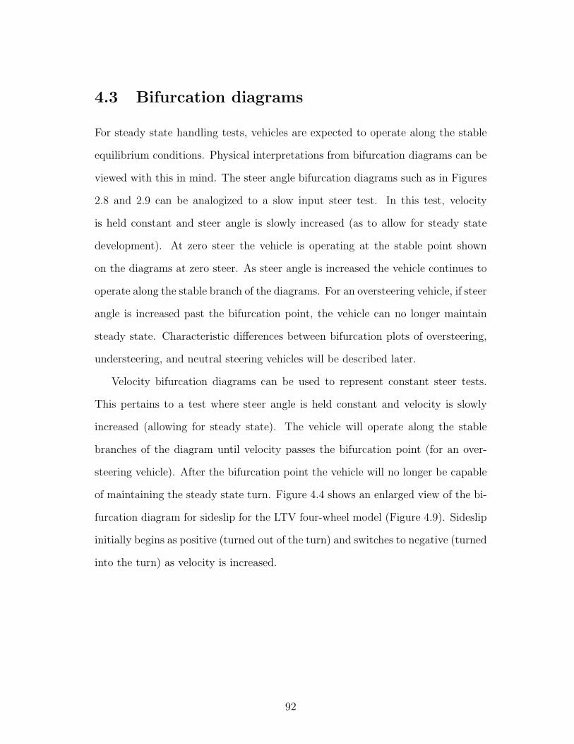
4.3 Bifurcation diagrams
For steady state handling tests, vehicles are expected to operate along the stable
equilibrium conditions. Physical interpretations from bifurcation diagrams can be
viewed with this in mind. The steer angle bifurcation diagrams such as in Figures
2.8 and 2.9 can be analogized to a slow input steer test. In this test, velocity
is held constant and steer angle is slowly increased (as to allow for steady state
development). At zero steer the vehicle is operating at the stable point shown
on the diagrams at zero steer. As steer angle is increased the vehicle continues to
operate along the stable branch of the diagrams. For an oversteering vehicle, if steer
angle is increased past the bifurcation point, the vehicle can no longer maintain
steady state. Characteristic differences between bifurcation plots of oversteering,
understeering, and neutral steering vehicles will be described later.
Velocity bifurcation diagrams can be used to represent constant steer tests.
This pertains to a test where steer angle is held constant and velocity is slowly
increased (allowing for steady state). The vehicle will operate along the stable
branches of the diagram until velocity passes the bifurcation point (for an over-
steering vehicle). After the bifurcation point the vehicle will no longer be capable
of maintaining the steady state turn. Figure 4.4 shows an enlarged view of the bi-
furcation diagram for sideslip for the LTV four-wheel model (Figure 4.9). Sideslip
initially begins as positive (turned out of the turn) and switches to negative (turned
into the turn) as velocity is increased.
92

Figure 4.4: Zoomed in view of bifurcation diagram for LTV 4 wheel model, equi-
librium values of β versus speed.
4.4 Understeer and neutral steer
The theoretical and LTV-based models presented thus far can be classified as
oversteering (in the forward direction). The bifurcations observed intuitively agree
with this classification. As steer angle or velocity was increased, the stable point
disappeared and the vehicle exceeded the practical operating limits, causing spin
out. Bifurcation behavior was found to be different for US and NS vehicles, as will
be discussed in the following section. Supporting theory for understeer, oversteer,
and neutral steer with nonlinear tire models is presented at the end of this chapter
for clarity.
93

4.4.1 Understeer
To better understand understeering bifurcation dynamics, an understeering vehicle
was created. The understeering model was based on the LTV four-wheel model.
To simplify the modifications, the simulation was run with 50 psi front and rear
tire pressure. The US/OS/NS classification is dependent on the normalized tire
force curves which are dependent on the tire forces and the axle weights. With
the same tires front and rear, US/NS/OS was controlled by simply adjusting the
weight by changing the CG location.
The LTV model was run with the same vehicle parameters except for the
longitudinal CG location. The dimensions af and ar were interchanged, so af =
1.4961 and ar = 1.8059. This moved the CG location closer to the front axle.
Figure 4.5 shows a low-speed phase portrait for the understeering model with the
same simulation parameters as in the earlier LTV model. Similar to the rear
facing direction in the expanded model, there exists five equilibrium points at low-
speed, one stable, two saddle and two unstable points. Figure 4.6 shows the same
understeering model at higher speed. Only the stable point remains. Intuitively
this agrees with the behavior of an understeering vehicle. As velocities and slip
angles increase, the front tires reach their limits and are no longer able to produce
sufficient force while the rear tires are still capable of creating a stabilizing moment.
The vehicle can be thought of as ’plowing’ out of the turn. Unlike the oversteering
case, a stable equilibrium position in the forward direction was always present.
94

Figure 4.5: Low speed, understeering phase plot.
Figure 4.6: High speed, understeering phase plot.
95

4.4.2 Neutral steer
In a similar manner to the understeering case, a neutral steering vehicle was created
from the LTV model. By setting af = ar = 1.651 and running the 50 psi tire
model for all four wheel corners, the front and rear normalized tire force curves
were exactly the same. So, αf = αr for any of the equilibrium points, and front
steer angle was simply the Ackerman steer angle. Figure 4.7 shows the neutral
steering phase plot at low speed. The plot is very similar to the oversteering case
with the same three equilibrium points. Figure 4.8 shows the high-speed neutral
steering case. Two equilibrium solutions still exist, however trajectories leading to
the stable point are not apparent. This qualitatively means that the stable point
is a weak attractor or a “weakly” stable point (small real part of the eigenvalues).
More will be discussed about this in the following section.
Figure 4.7: Low speed, neutral steering phase plot.
96

Figure 4.8: High speed, neutral steering phase plot.
4.4.3 US/OS/NS bifurcation diagrams
Figures 4.9 and 4.10 are the bifurcation diagrams presented for the four-wheel
model presented in chapter 3. As mentioned earlier the vehicle parameters used
in these models produce an oversteering vehicle. As velocity is increased past
the bifurcation value for velocity, the stable equilibrium (the operating point for
steady-state handling) disappears leaving no stable solution.
Figures 4.11 and 4.12 are the bifurcation plots for the understeering model.
As velocity was increased, the saddle points and the unstable equilibrium points
converge to form two separate saddle node bifurcations. Bifurcations occur at
different values for velocity. However, since the bifurcations only involve the un-
stable/nonstable points, they are not as physically significant as the saddle node
bifurcation found in the oversteering case. The most important note for the under-
steering model was that the stable equilibrium solution does not see a bifurcation,
97

so the system is inherently stable in pure understeer.
Figures 4.13 and 4.14 are the bifurcation diagrams for the neutral steering
case. The stable equilibrium and one saddle node appear to converge. The branch
that continues represents the weak attracting/repulsing equilibrium point seen in
the phase portraits. The eigenvalues along the branch were shown to have real
parts very close to zero. This refers to the “drift” condition for neutral steering
vehicles when all four tires are saturated. The drop in the sideslip plot for the
stable equilibrium (before converging with the saddle point) was attributed to an
abrupt change in tire force characteristics. This was due to the front and rear
tires saturating together, since in the neutral case the front and rear sideslips, for
steady-state, are equal.
Figure 4.9: Bifurcation diagram for LTV 4 wheel model, equilibrium values of β
versus speed.
98
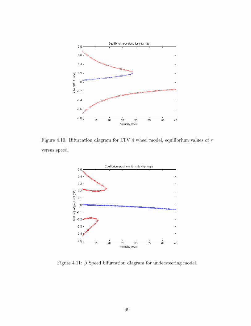
Figure 4.10: Bifurcation diagram for LTV 4 wheel model, equilibrium values of r
versus speed.
Figure 4.11: β Speed bifurcation diagram for understeering model.
99

Figure 4.12: r Speed bifurcation diagram for understeering model.
Figure 4.13: β Speed bifurcation diagram for neutral steering model.
100
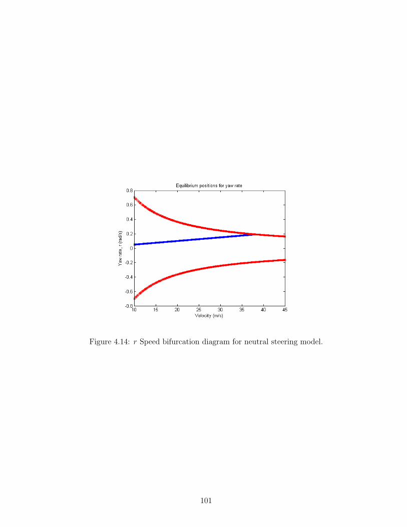
Figure 4.14: r Speed bifurcation diagram for neutral steering model.
101

4.5 Expanded model results
The rearward facing direction in the expanded model can be analogized to a for-
ward facing understeering vehicle. Although the vehicle in this condition was in
fact rear wheel steering, the tire and vehicle characteristics can still be used to de-
fine its steady-state behavior. The bifurcations observed in a conventional forward
facing, understeering, front-steer vehicle can be seen in the rear facing direction of
the expanded model. The most important similarity is that the stable equilibrium
in the rear facing direction exists at all speeds. This section discusses stability
notions for the expanded model and outlines some drawbacks in correlating this
model to practical vehicle maneuvers.
4.5.1 General stability versus practical stability
The expanded model extended the phase portrait outside of normal operational
limits to include dynamics such as backward-facing motion. The extended phase
portraits allow for analysis regarding overall system stability in the analytic sense.
Vehicles exceeding normal operating limitations may still be analytically stable.
For instance, the trajectory highlighted in Figure 4.15 shows vehicle motion that
would be considered unstable in the practical sense, but is still stable in terms of
the system equations (bounded). The vehicle in this case begins outside the stable
manifold for the forward facing stable equilibrium. The vehicle eventually rotates
past −90◦ of sideslip. In a system sense, the trajectory is stable since it remains
bounded as it eventually ends up at a rear-facing stable equilibrium point. Figure
4.16 shows the orientation plot for the trajectory highlighted in Figure 4.15. The
stable rear-facing equilibrium solution can be clearly seen as the vehicle eventually
reaches steady-state.
102

Figure 4.15: Phase portrait for extended LTV model at V = 27 m/s.
Another example can be shown post-bifurcation in the forward direction. Fig-
ure 4.17 is the phase portrait for the model at V = 36 m/s. In this case the
highlighted trajectory is initiated under conditions where there exists no stable
equilibrium in the forward direction. The trajectory then migrates to the rear-
ward facing stable equilibrium. Figure 4.18 shows the orientation plot for the
trajectory highlighted. The vehicle can be observed initially spinning and finally
reaching a steady condition in the backward direction.
The phase plots are repeating along the β direction, so any bounded initial
condition for β is analogous to the [−π, π] window. However the phase plane is
not repeated along the yaw rate direction. Figure 4.19 is an orientation plot for a
vehicle that starts with a very high yaw rate. The vehicle spins a few times and
103

Figure 4.16: Orientation plot for trajectory highlighted in V = 27 m/s phase plot.
finally reaches steady state at one of the backward facing equilibrium points. This
is an example of how bounded yaw rate initial conditions will eventually decay and
end up at one of the stable equilibrium points. This can be attributed to the tires
acting as yaw dampers slowing the rotational motion with time. This shows an
overall qualitative system stability for bounded initial conditions.
104

Figure 4.17: Phase portrait for extended LTV model at V = 36 m/s.
105

Figure 4.18: Orientation plot for trajectory highlighted in V = 36 m/s phase plot.
106
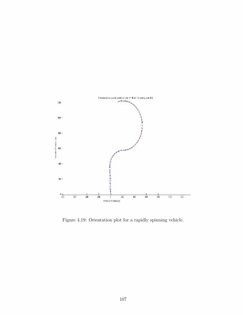
Figure 4.19: Orientation plot for a rapidly spinning vehicle.
107

4.5.2 Practicality of constant velocity assumptions
Although the extended model shows the vehicle system as being overall stable (for
bounded initial conditions), there are some drawbacks to viewing the vehicle with
this model. Vehicle motion in the state space is bounded, but the state approach
only considers motion relative to the vehicle reference frame. In practice, a fixed
reference frame, such as the one used for the orientation plots (motion with respect
to the road coordinates), is more practical. Also, when considering forward motion,
excessive sideslips and backward motion should not be considered as a “stable”
motions.
Another drawback to the method is the constant velocity magnitude condition.
In all of the models, the velocity magnitude was considered constant. Tire forces
in the direction of the velocity are neglected. As with yaw, tire forces (unless bal-
anced) are expected to reduce velocity when slip angles are present. This is due to
the fact that slip angles generate tire force components that oppose velocity. The
deceleration in the direction of velocity is assumed to be balanced by the driving
torque of the vehicle. When vehicle sideslip is small, forward drive torque can
adequately oppose the tire force. As sideslip increases (and ultimately at ±90◦
sideslip for a RWD vehicle) the drive torque can no longer be expected to pro-
vide any appreciable force in the direction of velocity. Also, drive torque cannot
be expected to provide force solely in the direction of velocity. When the vehicle
begins to face backward, the driving force must switch from forward to backward
in order to counter tire resistance. In a real-world maneuver, reaching a rear-
ward facing equilibrium from a forward facing initial condition requires switching
from forward driving torque to reverse driving torque. These conditions are not
practical. Instead, these trajectories can be thought of as pertaining to transient
108

spinouts, where the vehicle carries speed through the maneuver (tire forces don’t
appreciably reduce the velocity magnitude).
4.6 Lateral load model
The lateral load model is difficult to analyze using only the β-r plane. The state
space plane is only a projection of the entire set of system states. β and r no longer
fully define the vehicle operating state. A vehicle operating at a particular β and
r can still be operating at an infinite number of roll angles, roll rates, and tire
lateral forces. However, even with propagations external to the projected plane,
system tendencies can still be observed in the phase portraits. Trajectories can
be observed migrating towards the stable equilibrium and travelling towards and
away from the saddle points. Equilibrium solutions in this model show vehicle
motion (β and r) at steady state under a dynamic lateral loading condition.
Further exploration of the lateral load model is left for future work, where a
time animation might help describe and visualize system dynamics for different
initial conditions. In addition, a possible alternative model is presented later in
Chapter 5.
4.7 Nonlinear steady-state handling classification
For the nonlinear regimes of performance, the qualitative definitions of steady-state
US/OS/NS are the same as in the linear model presented in chapter 1. US/OS/NS
can be physically described when requiring more or less steer angle as (as compared
to the Ackerman steer angle) velocity is increased. In this analysis, steady-state
classification is performed in only the positive yaw direction, although the analysis
109

can be applied in a similar manner to the opposite direction. Again practical
US/OS/NS definitions relate to local rate of change of steer angle. If steer angle
is increasing (regardless of it’s relationship to the Ackerman steer angle) when
velocity increases, the vehicle can be considered as understeering. If the steer
angle is decreasing, the vehicle is oversteering.
As with the classification presented in chapter 1, it is easiest to work with a
bicycle vehicle model. Revisiting equations (2.7) and (2.9) for the bicycle model,
front steer angle can be rewritten as Eq. (4.1). From Eqs. (2.8), and (2.10), β can
be written as Eq. (4.2). Eqs. (4.1) and (4.2) can then be combined to create a
representation of front steer angle in terms of αf and αr, as given in Eq. (4.3). For
a constant radius turn, r = V/R describes the relationship between velocity, V ,
turn radius, R, and yaw rate r. Substituting this relationship into Eq. (4.3) puts
all the terms in a form similar to the analysis in chapter 1, as shown in Eq. (4.4).
δf = β − tan−1
(afrcos(β)
V
)− αf (4.1)
β = tan−1
(arrcos(β)
V
)+ αr (4.2)
δf = tan−1
(arrcos(β)
V
)− tan−1
(afrcos(β)
V
)+ αr − αf (4.3)
δf = tan−1
(arcos(β)
R
)− tan−1
(afcos(β)
R
)+ αr − αf (4.4)
The first terms in the expression for front steer angle, tan−1(
arcos(β)R
)−tan−1
(af cos(β)
R
),
can be thought of as the Ackerman steer angle. With a few small angle approxima-
tions for β and a(f/r)/R, and the Ackerman steer angle simplifies to the familiar
L/R (the same form used in the linear tire analysis). With either representa-
tion, the Ackerman steer angle is constant with respect to the vehicle and turn
parameters, therefore the only term of interest is (αr − αf ).
The sign of this term is opposite from the analysis in Chapter 1. This can
110
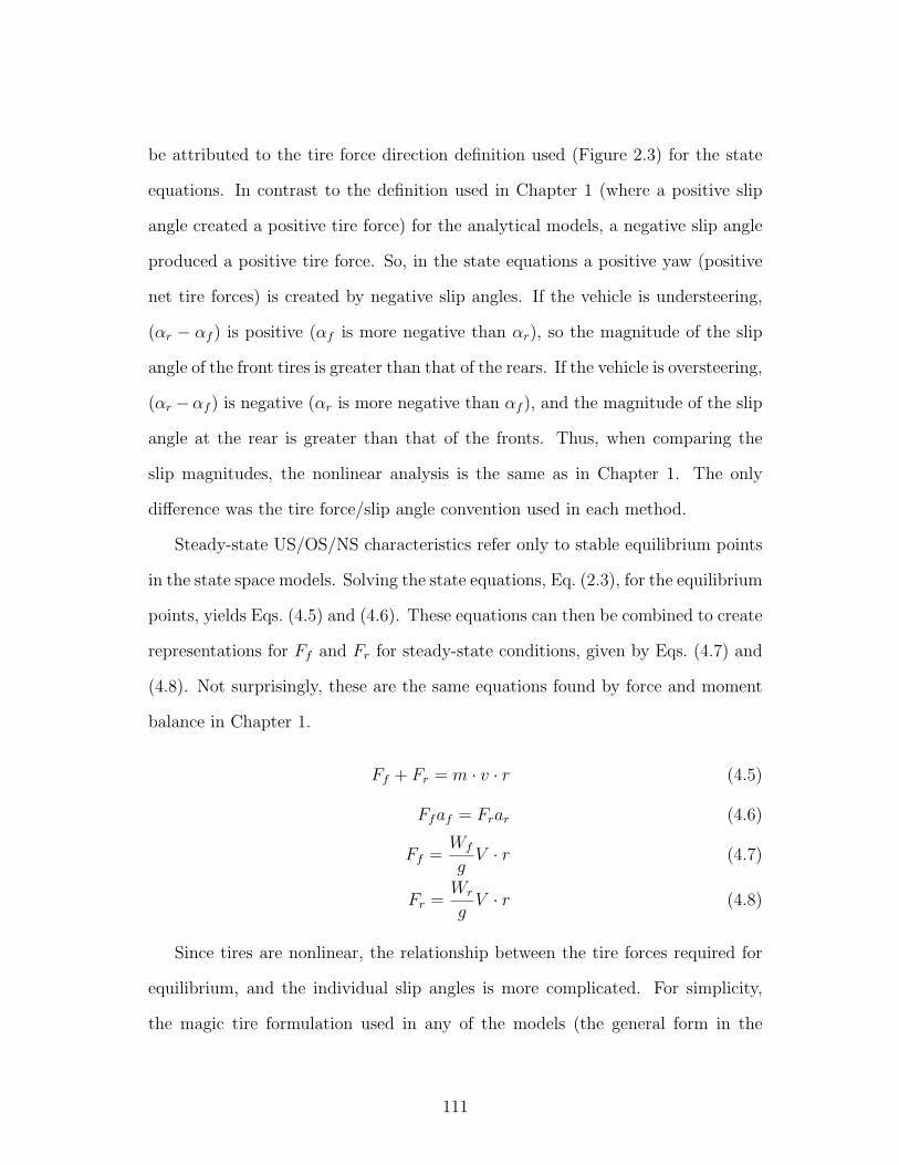
be attributed to the tire force direction definition used (Figure 2.3) for the state
equations. In contrast to the definition used in Chapter 1 (where a positive slip
angle created a positive tire force) for the analytical models, a negative slip angle
produced a positive tire force. So, in the state equations a positive yaw (positive
net tire forces) is created by negative slip angles. If the vehicle is understeering,
(αr − αf ) is positive (αf is more negative than αr), so the magnitude of the slip
angle of the front tires is greater than that of the rears. If the vehicle is oversteering,
(αr −αf ) is negative (αr is more negative than αf ), and the magnitude of the slip
angle at the rear is greater than that of the fronts. Thus, when comparing the
slip magnitudes, the nonlinear analysis is the same as in Chapter 1. The only
difference was the tire force/slip angle convention used in each method.
Steady-state US/OS/NS characteristics refer only to stable equilibrium points
in the state space models. Solving the state equations, Eq. (2.3), for the equilibrium
points, yields Eqs. (4.5) and (4.6). These equations can then be combined to create
representations for Ff and Fr for steady-state conditions, given by Eqs. (4.7) and
(4.8). Not surprisingly, these are the same equations found by force and moment
balance in Chapter 1.
Ff + Fr = m · v · r (4.5)
Ffaf = Frar (4.6)
Ff =Wf
gV · r (4.7)
Fr =Wr
gV · r (4.8)
Since tires are nonlinear, the relationship between the tire forces required for
equilibrium, and the individual slip angles is more complicated. For simplicity,
the magic tire formulation used in any of the models (the general form in the
111
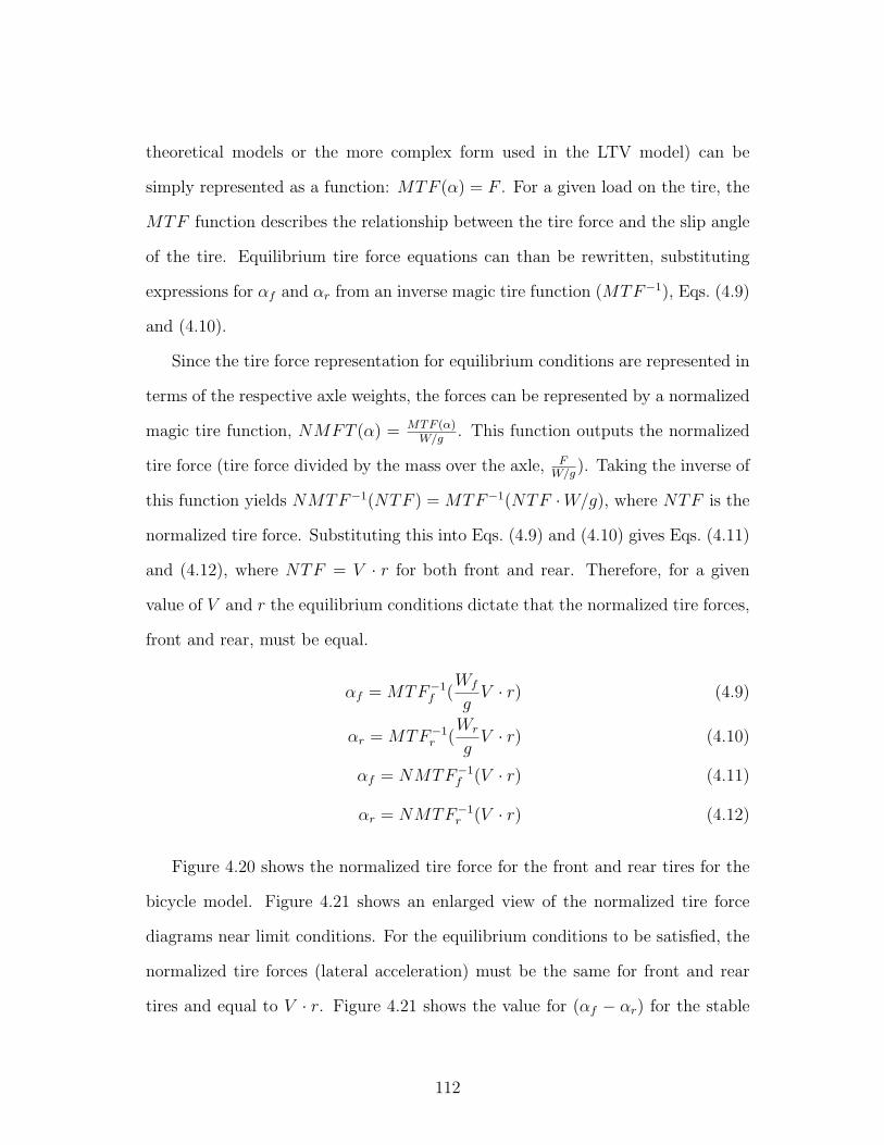
theoretical models or the more complex form used in the LTV model) can be
simply represented as a function: MTF (α) = F . For a given load on the tire, the
MTF function describes the relationship between the tire force and the slip angle
of the tire. Equilibrium tire force equations can than be rewritten, substituting
expressions for αf and αr from an inverse magic tire function (MTF−1), Eqs. (4.9)
and (4.10).
Since the tire force representation for equilibrium conditions are represented in
terms of the respective axle weights, the forces can be represented by a normalized
magic tire function, NMFT (α) = MTF (α)W/g
. This function outputs the normalized
tire force (tire force divided by the mass over the axle, FW/g
). Taking the inverse of
this function yields NMTF−1(NTF ) = MTF−1(NTF ·W/g), where NTF is the
normalized tire force. Substituting this into Eqs. (4.9) and (4.10) gives Eqs. (4.11)
and (4.12), where NTF = V · r for both front and rear. Therefore, for a given
value of V and r the equilibrium conditions dictate that the normalized tire forces,
front and rear, must be equal.
αf = MTF−1f (
Wf
gV · r) (4.9)
αr = MTF−1r (
Wr
gV · r) (4.10)
αf = NMTF−1f (V · r) (4.11)
αr = NMTF−1r (V · r) (4.12)
Figure 4.20 shows the normalized tire force for the front and rear tires for the
bicycle model. Figure 4.21 shows an enlarged view of the normalized tire force
diagrams near limit conditions. For the equilibrium conditions to be satisfied, the
normalized tire forces (lateral acceleration) must be the same for front and rear
tires and equal to V · r. Figure 4.21 shows the value for (αf − αr) for the stable
112

equilibrium point for a given value of V ·r. In this near limit condition, αr < αf , so
(αr −αf ) is negative and the vehicle is steered less than the Ackerman steer angle
(exhibiting oversteer). It can also be noted that as lateral acceleration is increased
(V · r is increased), (αr−αf ) becomes even more negative (αf −αr on the diagram
grows wider). Figure 4.22 is a plot of (αr − αf ) versus lateral acceleration. Near
the limit (high lateral accelerations) the slope of the curve is negative, indicating
that increases in lateral acceleration lead to decreases in (αr − αf ) which in turn
means decreases the front steer angle (Eq. (4.4). The vehicle, near limit, can also
be considered oversteering in the practical sense (showing increasing oversteer).
One interesting note is that for the theoretical bicycle model, at the lower lateral
accelerations, both (αr − αf ) and the slope are positive. This means that the
vehicle initially understeers in the analytical and practical sense. The vehicle then
transitions into oversteer near limit. The remaining theoretical models are based
on the bicycle model tire forces, so similar analysis provides the same oversteering
results for the tandem, and four-wheel theoretical models.
Figure 4.23 shows the normalized tire force curves for the tires and vehicle
parameters used in the LTV four-wheel model. Figure 4.24 shows the (αr − αf )
versus lateral acceleration plot. The values for (αr−αf ) are negative so the vehicle
is always exhibiting oversteer. Furthermore the slope of the curve is also always
negative, so the vehicle shows increasing oversteer and can also be considered
always oversteering in the practical sense.
113
Figure 4.20: Normalized tire force for bicycle model.
Figure 4.21: Zoomed in view of normalized tire force forbicycle model.
114

Figure 4.22: (αr − αf ) versus normalized tire force for theoretical bicycle model.
Figure 4.23: Normalized tire force for LTV four-wheel model.
115

Figure 4.24: (αr − αf ) versus normalized tire force for LTV four-wheel model.
116
Chapter 5
Summary and recommendations for future work
This research presented a new method to study vehicle handing performance. Ve-
hicle models evolved from a simple bicycle model to models allowing for wide oper-
ating ranges and lateral load transfer. US/OS/NS was explored for the nonlinear
case, and examples of bifurcation analysis were applied.
In addition to characterizing vehicle handing performance, this method can also
be used (to an extent) to predict vehicle motions for particular steering maneuvers.
For example, Figure 5.1 shows a graph provided by Ivan Tong from the US Army
Aberdeen Test Center (ATC) that shows a phase portrait overlayed with a curve
of stable equilibrium points at several other steer angles (black line). Trajectories
crossing the black line represent initial responses to a step steer input from the
equilibrium steering state at each point on the black line to the steer angle of the
phase portrait. Phase portraits also provide responses of steady vehicle parameters
after transient maneuvers.
Bifurcation plots can be used to determine stability limits for different vehicle
conditions. Vehicle specifications can be varied, and changes in handling behavior
can be easily evaluated. The lateral load model is especially powerful in this regard,
since simple changes such as roll bar adjustments can be examined. Homoclinic
117
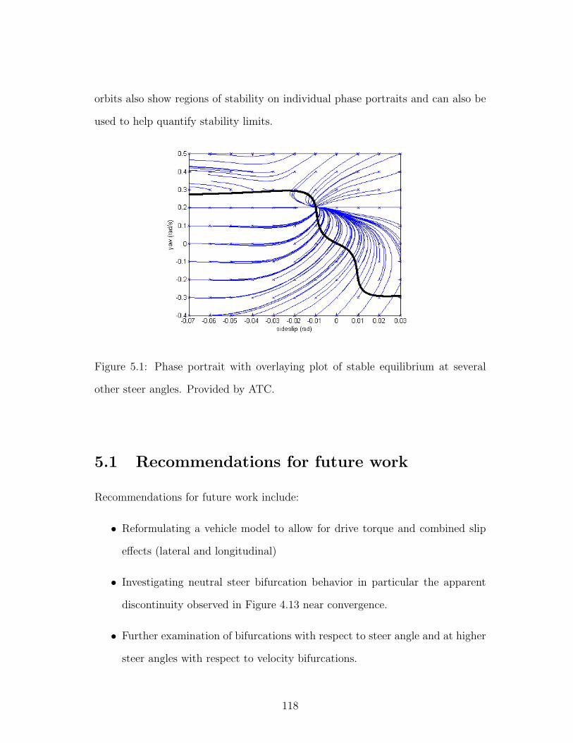
orbits also show regions of stability on individual phase portraits and can also be
used to help quantify stability limits.
Figure 5.1: Phase portrait with overlaying plot of stable equilibrium at several
other steer angles. Provided by ATC.
5.1 Recommendations for future work
Recommendations for future work include:
• Reformulating a vehicle model to allow for drive torque and combined slip
effects (lateral and longitudinal)
• Investigating neutral steer bifurcation behavior in particular the apparent
discontinuity observed in Figure 4.13 near convergence.
• Further examination of bifurcations with respect to steer angle and at higher
steer angles with respect to velocity bifurcations.
118
• Further development of the lateral load model, by perhaps removing initial
roll angle propagation or using animation in three dimensions for improved
visualization of system dynamics.
119

BIBLIOGRAPHY
[1] Ahmadi, J., Ghaffari, A., and Kazemi, R., 2005, “Fuzzy logic based
vehicle stability enhancement through combined defferential braking
and active front steering,” ASME DETC2005-85340, pp. 1-7.
[2] 2005, “Auto Alliance, Driving Innovation,”
http://www.autoalliance.org/safety/.
[3] Cabrera, J. A., Ortiz, A., Carabias, E., and Simon, A., 2004, “An
Alternative Meathod to Determine the Magic Tyre Model Parame-
ters Using Genetic Algorithms,” Vehicle System Dynamics, 41(2),
pp. 109-127.
[4] Chengrong, H., Feisheng, Z., 1994, “The numerical bifurcation
method of nonlinear lateral stability analysis of a locomotive,” Ve-
hicle System Dynamics, 23, pp. 234-245.
[5] Forkenbrock, G., and Garrott, R., 2005, “NHTSA Vehi-
cle Research and Test Center CRASH AVOIDANCE RE-
SEARCH Vehicle Dynamic Rollover Propensity”, http://www-
nrd.nhtsa.dot.gov/vrtc/ca/rollover.htm.
120

[6] Forkenbrock, G., 2005, “An overivew of NHTSA’s 2005 ESC research
program,” Ninteenth International Confrence on Enhanced Safety of
Vehicles, presentation notes.
[7] Ghaffari, A., Ahmadi, J., and Kazemi, R., 2005, “Fuzzy logic based
vehicle stability enhacement through active rear steering,” ASME
DETC2005-85350, pp. 1-7.
[8] Gillespie, T.D. 1992, Fundamentals of Vehicle Dynamics, Society of
Automotive Engineers, Warrendale, PA.
[9] Huh, K., Kim, J., Hong, J., 2000, “Handling and driving character-
istics for six-wheeled”, Proc. Instn. Mech. Eng. Vol. 214 Part D, pp.
159-170.
[10] Karnopp D., 2004, Vehicle Stability (New York: Marcel Dekker).
[11] Klaps, J., Day, A. J., 2005, “Steering drift and wheel movements
during rbaking: static and dynamic measurements,” Proc. Instn.
Mech. Eng. Vol. 219 Part D:J. Automobile Engineering, pp. 11-19.
[12] Lv, H. M., Chen, N., Li, P., 2004, “Multi-objective H∞ optimal
control for four-wheel steering vehicle based on yaw rate tracking,”
Proc. Instn. Mech. Eng. Vol. 218 Part D:J. Automobile Engineering,
pp. 1117-1123.
[13] M. van Oosten, J. J., and Bakker, E., 1993, “Determination of Magic
Tyre Model Parameters,” Tyre Models For Vehicle Dynamics Anal-
ysis, H. B. Pacejka eds., Offsetdrukkerij Kanters, Netherlands, pp.
19-29.
121
[14] Matlab Tutorial, 2005, Matlab ver. 7.0.4.365 (R14).
[15] Milliken, W.F., Milliken, D.L., 1995, Race Car Vehicle Dynamics,
Society of Automotive Engineers, Warrendale, PA.
[16] Mokhiamar, O., Abe, M., 2002, “Combined lateral force and yaw
moment control to maximize stability as well as vehicle responsive-
ness during evasive maneuvering for active vehicle handing safety,”
Vehicle System Dynamics, supplement 37, pp. 246-256.
[17] Nayfeh, A. H., Balachandran, B., 1995, Applied Nonlinear Dynam-
ics, analytical, computational, and experimental methods, John Wi-
ley & Sons, Inc., New York, Chap. 1-2.
[18] Ono E., Hosoe S., Tuan H. D., and Doi S., 1998, “Bifurcation in
vehicle dynamics and robust front wheel steering control,” IEEE
Transactions on Control Systems Technology, 6(3), pp. 412-420.
[19] Pacejka, H. B., Bakker, E., 1993, “The Magic Formula Tyre Model,”
Tyre Models For Vehicle Dynamics Analysis, H. B. Pacejka eds.,
Offsetdrukkerij Kanters, Netherlands, pp. 1-18.
[20] Sharp, R. S., “Normalization of tire shear forces for economy of
testing and computation,” 2005, Obtained directly from author.
[21] Sharp, R. S., 2005 “Testing and improving a tyre shear force com-
putation algorithm,” 2005, Obtained directly from author.
[22] Sharp, R. S., and Bettella, M., 2003, “Tyre Shear Force and Mo-
ment descriptions by Normalization of Parameters and the ‘Magic
Formula’,” Vehicle System Dynamics, 39(1), pp. 27-56.
122

[23] Sharp, R. S., and Bettella, M., 2003, “On the construction of a
general numerical tyre shear force model from limited data,” Journal
of Automobile Engineering, 217 Proc. I. Mech. E., Part D., pp. 165-
172.
[24] Yi, K., Chung, T., Kim, J., and Yi, S., 2003, “An investigation into
differential braking strategies for vehicle stability control,” Proc.
Instn. Mech. Eng. Vol. 217 Part D: J. Automobile Engineering, pp.
1081-1093.
123