ABSTRACT Title of Dissertation: VEHICLE BRIDGE INTERACTION ...
284
ABSTRACT Title of Dissertation: VEHICLE BRIDGE INTERACTION ANALYSIS ON CONCRETE AND STEEL CURVED BRIDGES Yunchao Ye, Ph.D. of Civil Engineering, 2019 Dissertation Directed By: Professor Chung C. Fu, Ph.D., P.E. Civil and Environmental Engineering This study investigation is intended to research the dynamic reactions of horizontally curved bridge under heavy vehicle load. Most of the main factors that affect the bridge dynamic response due to moving vehicles are considered. First, an improved grid model is developed for the analysis of curved bridges based on the shear-flexibility grillage analyzing method, in which the effects of warping stiffness and moment of inertia are both considered. Based on commercial software ANSYS Mechanical APDL, 3D beam element, mass element and spring-damper element are integrated together in building a 3D vehicle and bridge system. A simplified numeric method is developed for solving the interaction problem, considering the effect of
Transcript of ABSTRACT Title of Dissertation: VEHICLE BRIDGE INTERACTION ...

ABSTRACT
Title of Dissertation:
VEHICLE BRIDGE INTERACTION
ANALYSIS ON CONCRETE AND STEEL
CURVED BRIDGES
Yunchao Ye, Ph.D. of Civil Engineering,
2019
Dissertation Directed By:
Professor Chung C. Fu, Ph.D., P.E.
Civil and Environmental Engineering
This study investigation is intended to research the dynamic reactions of horizontally
curved bridge under heavy vehicle load. Most of the main factors that affect the bridge
dynamic response due to moving vehicles are considered.
First, an improved grid model is developed for the analysis of curved bridges based
on the shear-flexibility grillage analyzing method, in which the effects of warping
stiffness and moment of inertia are both considered. Based on commercial software
ANSYS Mechanical APDL, 3D beam element, mass element and spring-damper element
are integrated together in building a 3D vehicle and bridge system. A simplified numeric
method is developed for solving the interaction problem, considering the effect of

random road roughness and its velocity term. This system is tested on two case study
bridges, Manchuria concrete bridge and Veteran’s Memorial steel bridge.
Second, with the model and numerical method presented, a series of parametric
studies are conducted to study during the curved bridge dynamic interaction. In the study,
the effects of curvature of radius, bridge surface roughness, bridge span configuration,
traffic lane eccentricities and speed are investigated and analyzed. The dynamic response
and dynamic impact factors are calculated and compared. The analysis results provide
good references for the stipulation of impact factor formulae in the later studies.
Third, based on the investigation of determining factors of curve bridge dynamic
interaction, the expression for upper-bound envelop for impact factors of maximum
deflection is given in different surface conditions and highway speed limits as a function
of bridge fundamental frequency or bridge central angle. A study is conducted on
comparing this empirical equation and serval other major design codes, comments and
suggestion are made based on the discoveries.

VEHICLE BRIDGE INTERACTION ANALYSIS ON CONCRETE AND STEEL
CURVED BRIDGES
by
Yunchao Ye
Dissertation submitted to the Faculty of the Graduate School of the
University of Maryland, College Park, in partial fulfillment
of the requirements for the degree of
Doctor of Philosophy
2019
Advisory Committee:
Professor Chung. C. Fu Advisor, Chair
Professor M. Sherif Aggour
Professor Amde M. Amde
Professor Brian M. Phillips
Professor Sung Lee

© Copyright by
Yunchao Ye
2019

ii
Acknowledgements
I would like to take this opportunity to thank my advisor, Dr. Chung C. Fu, for his kind
guidance during my studies. His advice was very crucial for the success of this work. I
have truly enjoyed my time working for him,
I also thank my committee members: Dr. Aggour, Dr. Amde, Dr. Phillip and Dr. Lee for
their valuable time reading my work and providing their insight and comments.
Financial support provided by Dr. Fu and the Bridge Engineering Software and
Technology (BEST) Center is gratefully acknowledged.
Finally, I would like to thank all my family members and my friends from BEST Center
for their patience and support throughout the course of this research.

iii
Table of Contents Acknowledgements............................................................................................ ii
1. Introduction .......................................................................................................... 1
1.1 Research Motivation ........................................................................................ 1
1.2 Background ...................................................................................................... 2
1.3 Research objective ............................................................................................ 5
2. Literature review .................................................................................................. 7
2.1 Vehicle model .................................................................................................. 7
2.2 Bridge model .................................................................................................. 11
2.3 Influence of horizontal curvature ................................................................... 13
2.4 Method of Solution ......................................................................................... 13
2.5 Damping influence ......................................................................................... 15
2.6 Impact factor .................................................................................................. 16
3. Research Outline ................................................................................................ 20
4. Theory of Vehicle-Bridge Analysis ................................................................... 22
4.1 Dynamic Analysis Model and Dynamic Characteristic Parameter Analysis of
Curved Girder Bridge ................................................................................................... 22
4.2 Multi-axis vehicle model description ............................................................. 26
4.2.1 Vehicle model coordinate systems ......................................................... 26

iv
4.2.2 Simplified vehicle model (3-axle) ....................................................... 27
4.2.3 Simplified vehicle model (3D, 3-axle) ................................................ 29
4.3 Random surface roughness ............................................................................. 30
4.4 Vehicle-Bridge coupling analysis .................................................................. 31
4.4.1 Basic assumptions ................................................................................... 31
4.4.2 Motion equations of vehicle ................................................................... 32
4.4.3 Motion equations of bridge ..................................................................... 33
4.4.4 Solution of vehicle bridge dynamic interaction force ............................. 33
5. Vehicle bridge interaction analysis and preliminary result ................................ 37
5.1 Case study bridge models ............................................................................... 37
5.1.1 Manchuria Interchange Bridge ............................................................... 37
5.1.2 Veteran’s Memorial Bridge .................................................................... 45
5.2 Preliminary case study results ........................................................................ 47
5.2.1 Manchuria Concrete Curved Bridge ....................................................... 47
5.2.2 Veteran’s Memorial Steel Curved Bridge .............................................. 59
5.3 Preliminary case study summary .................................................................... 64
6. Parametric Study ................................................................................................ 66
6.1 Introduction .................................................................................................... 66
6.2 Analysis Cases ................................................................................................ 66

v
7. Results of Parametric Study ............................................................................... 76
7.1 Introduction .................................................................................................... 76
7.2 Analysis Results ............................................................................................. 76
7.2.1 For 3 span configurations ....................................................................... 77
7.2.2 Curvature comparison study ................................................................... 78
7.2.3 Span lengths comparison study .............................................................. 88
7.2.4 Vehicle travelling speeds comparison study........................................... 92
7.2.5 Deck roughness comparison study ......................................................... 96
7.2.6 Eccentricity study ................................................................................. 102
7.2.7 For 2-span bridge configurations .......................................................... 104
7.3 Discussion of Results ................................................................................... 107
8. Calculation of Impact Factor ............................................................................ 118
8.1 Calculation based on bridge natural frequency ............................................ 118
8.2 Calculation based on bridge central angle .................................................... 130
9. Summary, Conclusions and Future Work ........................................................ 141
9.1 Summary and Conclusion ............................................................................ 141
9.1.1 Innovation in this study ........................................................................ 144
9.2 Suggestions for future Work ........................................................................ 145
10. Appendix -A ................................................................................................. 147

vi
11. Appendix – B ................................................................................................ 230
12. Appendix -C ................................................................................................. 244
13. Reference ...................................................................................................... 259

vii
List of Figures
Figure 1-1 Shangyu curved bridge accident ............................................................... 2
Figure 2-1 Moving load model ................................................................................... 8
Figure 2-2 Moving mass model .................................................................................. 9
Figure 2-3 Sprung mass model ................................................................................. 10
Figure 2-4 Multiple-axle truck model ....................................................................... 11
Figure 2-5 vehicle bridge interaction with surface roughness model ....................... 13
Figure 2-6 Dynamic load allowance in OHBDC ...................................................... 18
Figure 4-1 3-axle truck model and degrees of freedom ............................................ 28
Figure 4-2 3-axle truck model and degrees of freedom ............................................ 29
Figure 4-3 3D truck model ........................................................................................ 29
Figure 4-4 Centrifugal forces on the moving vehicle ............................................... 32
Figure 5-1 Manchuria bridge layout and cross section ............................................. 38
Figure 5-2 Dynamic Analysis models of the Curved Bridge- Simple beam model . 40
Figure 5-3 Dynamic Analysis models of the Curved Bridge- Triple-beam model ... 41
Figure 5-4 Dynamic Analysis models of the Curved Bridge- Solid finite element
model................................................................................................................................. 41
Figure 5-5 Typical 2-axle truck models used in the vehicle-bridge ......................... 42
Figure 5-6 Typical 3-axle truck models used in the vehicle-bridge ......................... 42
Figure 5-7 Typical 3D 3-axle truck models used in the vehicle-bridge analysis ...... 43
Figure 5-8 Roughness profiles of different types of deck (Good surface condition) 44

viii
Figure 5-9 Roughness profiles of different types of deck (Normal surface condition)
........................................................................................................................................... 44
Figure 5-10 Roughness profiles of different types of deck (Bad surface condition) 44
Figure 5-11 Veteran’s bridge layout and cross section ............................................. 46
Figure 5-12 Flange deflection of mid span (vehicle speed v=10m/s) ....................... 47
Figure 5-13 Flange deflection of mid span (vehicle speed v=20m/s) ....................... 48
Figure 5-14 Flange deflection of mid span (vehicle speed v=30m/s) ....................... 48
Figure 5-15 Flange deflection of mid span (vehicle speed v=40m/s) ....................... 49
Figure 5-16 Moment force response of mid span at v=10m/s .................................. 49
Figure 5-17 Moment force response of mid span at v=20m/s .................................. 50
Figure 5-18 Moment force response of mid span at v=30m/s .................................. 50
Figure 5-19 Moment force response of mid span at v=40m/s .................................. 51
Figure 5-20 Amplication factors of different traveling speeds. ................................ 52
Figure 5-21 Bridge girder deflection response of a 3-axle truck passing through the
bridge. ............................................................................................................................... 53
Figure 5-22 Bridge deflection response vs Good surface condition ......................... 53
Figure 5-23 Bridge deflection response vs Normal surface condition ...................... 54
Figure 5-24 Bridge deflection response vs Bad surface condition ........................... 54
Figure 5-25 Amplified factor vs different surface conditions................................... 55
Figure 5-26 Maximum deflections under different vehicle traveling speed and road
condition ........................................................................................................................... 56

ix
Figure 5-27 Impact factor of bridge under different vehicle traveling speed and road
condition ........................................................................................................................... 56
Figure 5-28 Moment response comparison between curved Manchuria Bridge and
hypothetical straight Manchuria Bridge............................................................................ 57
Figure 5-29 Z-displacements comparison between curved Manchuria Bridge and
hypothetical straight Manchuria Bridge............................................................................ 58
Figure 5-30 Impact factor comparison between curved Manchuria Bridge and
hypothetical straight Manchuria Bridge............................................................................ 58
Figure 5-31 Girder deflection of mid span (vehicle speed v=28m/s) ....................... 59
Figure 5-32 Girder deflection of mid span (vehicle speed v=32m/s) ....................... 60
Figure 5-33 Girder deflection of mid span (vehicle speed v=38m/s) ....................... 60
Figure 5-34 Moment force response of mid span (vehicle speed v=28m/s) ............. 61
Figure 5-35 Moment force response of mid span (vehicle speed v=32m/s) ............. 61
Figure 5-36 Moment force response of mid span (vehicle speed v=38m/s) ............. 62
Figure 5-37 Moment response comparison between curved Veteran’s Memorial
Bridge and hypothetical straight Veteran’s Memorial Bridge. ......................................... 63
Figure 5-38 Z-displacements comparison between curved Veteran’s Memorial Bridge
and hypothetical straight Veteran’s Memorial Bridge. ..................................................... 63
Figure 5-39 Impact factor comparison between curved Veteran’s Memorial Bridge
and hypothetical straight Veteran’s Memorial Bridge. ..................................................... 64
Figure 6-1 Good surface condition applied in parametric study ............................... 68
Figure 6-2 Normal surface condition applied in parametric study ........................... 68

x
Figure 6-3 Bad surface condition applied in parametric study ................................. 68
Figure 6-4 Typical steel box girder cross section (Case 1 L=175m). ....................... 69
Figure 6-5 Typical steel box girder cross section near pier location (Case 1 L=175m)
........................................................................................................................................... 69
Figure 6-6 Typical steel box girder cross section (Case 2 L=120m) ........................ 70
Figure 6-7 Typical steel box girder cross section near pier location (Case 2 L=120m)
........................................................................................................................................... 70
Figure 6-8 Typical steel box girder cross section (Case 3 L=235m) ........................ 71
Figure 6-9 Typical steel box girder cross section near pier location (Case 3 L=235m)
........................................................................................................................................... 71
Figure 6-10 Typical curved bridge layout ................................................................ 73
Figure 7-1 Mid-span displacement for 3-span bridge model R=50m ....................... 78
Figure 7-2 Mid-span shear force for 3-span bridge model R=50m .......................... 79
Figure 7-3 Mid-span moment for 3-span bridge model R=50m ............................... 79
Figure 7-4 Mid-span displacement for 3-span bridge model R=75m ....................... 80
Figure 7-5 Mid-span shear force for 3-span bridge model R=75m .......................... 80
Figure 7-6 Mid-span moment for 3-span bridge model R=75m ............................... 81
Figure 7-7 Mid-span displacement for 3-span bridge model R=100m ..................... 81
Figure 7-8 Mid-span shear force for 3-span bridge model R=100m ........................ 82
Figure 7-9 Mid-span shear force for 3-span bridge model R=100m ........................ 82
Figure 7-10 Mid-span displacement for 3-span bridge model R=150m ................... 83
Figure 7-11 Mid-span shear force for 3-span bridge model R=150m ...................... 83

xi
Figure 7-12 Mid-span shear force for 3-span bridge model R=150m ...................... 84
Figure 7-13 Mid-span displacement for 3-span bridge model R=190m ................... 84
Figure 7-14 Mid-span shear force for 3-span bridge model R=190m ...................... 85
Figure 7-15 Mid-span shear force for 3-span bridge model R=190m ...................... 85
Figure 7-16 Mid-span displacement for 3-span bridge model R=300m ................... 86
Figure 7-17 Mid-span shear force for 3-span bridge model R=300m ...................... 86
Figure 7-18 Mid-span shear force for 3-span bridge model R=300m ...................... 87
Figure 7-19 Mid-span displacement for 3-span bridge model L=175m ................... 88
Figure 7-20 Mid-span shear force for 3-span bridge model L=175m ...................... 88
Figure 7-21 Mid-span shear force for 3-span bridge model L=175m ...................... 89
Figure 7-22 Mid-span displacement for 3-span bridge model L=235m ................... 89
Figure 7-23 Mid-span shear force for 3-span bridge model L=235m ...................... 90
Figure 7-24 Mid-span shear force for 3-span bridge model L=235m ...................... 90
Figure 7-25 Mid-span displacement for 3-span bridge model L=120m ................... 91
Figure 7-26 Mid-span shear force for 3-span bridge model L=120m ...................... 91
Figure 7-27 Mid-span shear force for 3-span bridge model L=120m ...................... 92
Figure 7-28 Mid-span displacement for 3-span bridge model v=20m/s ................... 92
Figure 7-29 Mid-span displacement for 3-span bridge model v=30m/s ................... 93
Figure 7-30 Mid-span displacement for 3-span bridge model v=40m/s ................... 93
Figure 7-31 Mid-span displacement for 3-span bridge model v=50m/s ................... 94
Figure 7-32 Mid-span displacement for 3-span bridge model v=60m/s ................... 94
Figure 7-33 Mid-span displacement for 3-span bridge model v=70m/s ................... 95

xii
Figure 7-34 Mid-span displacement for 3-span bridge model v=30m/s L=235m
perfect surface condition ................................................................................................... 96
Figure 7-35 Mid-span displacement for 3-span bridge model v=30m/s L=235m good
surface condition ............................................................................................................... 96
Figure 7-36 Mid-span displacement for 3-span bridge model v=30m/s L=235m
normal surface condition................................................................................................... 97
Figure 7-37 Mid-span displacement for 3-span bridge model v=30m/s L=235m bad
surface condition ............................................................................................................... 97
Figure 7-38 Mid-span displacement for 3-span bridge model v=30m/s L=175m
perfect surface condition ................................................................................................... 98
Figure 7-39 Mid-span displacement for 3-span bridge model v=30m/s L=175m good
surface condition ............................................................................................................... 98
Figure 7-40 Mid-span displacement for 3-span bridge model v=30m/s L=175m
normal surface condition................................................................................................... 99
Figure 7-41 Mid-span displacement for 3-span bridge model v=30m/s L=175m bad
surface condition ............................................................................................................... 99
Figure 7-42 Mid-span displacement for 3-span bridge model v=30m/s L=120m
perfect surface condition ................................................................................................. 100
Figure 7-43 Mid-span displacement for 3-span bridge model v=30m/s L=120m good
surface condition ............................................................................................................. 100
Figure 7-44 Mid-span displacement for 3-span bridge model v=30m/s L=120m
normal surface condition................................................................................................. 101

xiii
Figure 7-45 Mid-span displacement for 3-span bridge model v=30m/s L=120m
normal surface condition................................................................................................. 101
Figure 7-46 Mid-span displacement for 3-span bridge model with vehicle traveling
through inner lane ........................................................................................................... 102
Figure 7-47 Mid-span displacement for 3-span bridge model with vehicle traveling
through center lane .......................................................................................................... 102
Figure 7-48 Mid-span displacement for 3-span bridge model with vehicle traveling
through outer lane ........................................................................................................... 103
Figure 7-49 Mid-span displacement for 2-span bridge model v=20m/s ................. 104
Figure 7-50 Mid-span displacement for 2-span bridge model v=30m/s ................. 104
Figure 7-51 Mid-span displacement for 2-span bridge model v=40m/s ................. 105
Figure 7-52 Mid-span displacement for 2-span bridge model v=50m/s ................. 105
Figure 7-53 Mid-span displacement for 2-span bridge model v=60m/s ................. 106
Figure 7-54 Mid-span displacement for 2-span bridge model v=70m/s ................. 107
Figure 7-55 Displacement reactions with different radii ........................................ 108
Figure 7-56 Differences of displacement increment ............................................... 109
Figure 7-57 mid-span moment comparison under different radii configurations ... 110
Figure 7-58 negative moment impact factors for different radii configurations..... 110
Figure 7-59 positive moment impact factors for different radii configurations ..... 111
Figure 7-60 mid-span displacement comparison under different span length
configurations ................................................................................................................. 112
xiv
Figure 7-61 displacement increment comparison under different span length
configurations ................................................................................................................. 112
Figure 7-62 Amplified factors vs. surface condition vs. vehicle (Normal span case)
......................................................................................................................................... 113
Figure 7-63 Impact factor of different surfaces and span configurations ............... 115
Figure 7-64 Amplified factors vs. surface condition vs. vehicle (Short span case) 116
Figure 7-65 Impact factor for different eccentricity ............................................... 117
Figure 8-1 Displacement impact factor versus bridge frequency (v=20m/s) for perfect
roughness ........................................................................................................................ 121
Figure 8-2 Displacement impact factor versus bridge frequency (v=30m/s) for perfect
roughness ........................................................................................................................ 121
Figure 8-3 Displacement impact factor versus bridge frequency (v=20m/s) for
wearing deck ................................................................................................................... 122
Figure 8-4 Moment impact factor versus frequency (v=20m/s) for perfect roughness
......................................................................................................................................... 123
Figure 8-5 Moment Impact factor versus bridge frequency (v=30m/s) for perfect
roughness ........................................................................................................................ 124
Figure 8-6 Impact factor versus bridge frequency (v=20m/s) for wearing deck .... 124
Figure 8-7 Torsional impact factor versus frequency (v=20m/s) for perfect roughness
......................................................................................................................................... 125
Figure 8-8 Torsional impact factor versus frequency (v=30m/s) for perfect roughness
......................................................................................................................................... 126

xv
Figure 8-9 Torsional impact factor versus bridge frequency (v=20m/s) for wearing
deck ................................................................................................................................. 126
Figure 8-10 Shear impact factor versus frequency (v=20m/s) for perfect roughness
......................................................................................................................................... 127
Figure 8-11 Shear impact factor versus frequency (v=30m/s) for perfect roughness
......................................................................................................................................... 128
Figure 8-12 Shear impact factor versus bridge frequency (v=20m/s) for wearing deck
......................................................................................................................................... 128
Figure 8-13 Comparison of different methods of determining impact factors ....... 130
Figure 8-14 Displacement Impact factor versus bridge central angle (v=20m/s) for
perfect roughness ............................................................................................................ 133
Figure 8-15 Displacement Impact factor versus bridge central angle (v=30m/s) for
perfect roughness ............................................................................................................ 133
Figure 8-16 Displacement Impact factor versus bridge frequency (v=20m/s) for
wearing deck ................................................................................................................... 134
Figure 8-17 Moment impact factor versus bridge central angle (v=20m/s) for perfect
roughness ........................................................................................................................ 135
Figure 8-18 Moment impact factor versus bridge central angle (v=30m/s) for perfect
roughness ........................................................................................................................ 135
Figure 8-19 Moment impact factor versus bridge central angle (v=20m/s) for wearing
deck ................................................................................................................................. 136

xvi
Figure 8-20 Torsional impact factor versus bridge central angle (v=20m/s) for perfect
roughness ........................................................................................................................ 137
Figure 8-21 Torsional impact factor versus bridge central angle (v=30m/s) for perfect
roughness ........................................................................................................................ 137
Figure 8-22 Torsional impact factor versus bridge central angle (v=20m/s) for wearing
deck ................................................................................................................................. 138
Figure 8-23 Shear impact factor versus bridge central angle (v=20m/s) for perfect
roughness ........................................................................................................................ 139
Figure 8-24 Shear impact factor versus bridge central angle (v=30m/s) for perfect
roughness ........................................................................................................................ 139
Figure 8-25 Torsional impact factor versus bridge central angle (v=20m/s) for wearing
deck ................................................................................................................................. 140

xvii
List of Tables
Table 2-1 Dynamic load allowance in AASHTO LRFD Bridge Design Specification
........................................................................................................................................... 17
Table 5-1 Section properties of bridge model ........................................................... 38
Table 5-2 Section property of triple-beam model ..................................................... 40
Table 5-3 Section properties of bridge model ........................................................... 46
Table 6-1 Typical section properties for different span length bridge models. ........ 72
Table 6-2 Typical near pier section properties for different span length bridge models.
........................................................................................................................................... 72
Table 6-3 3-span bridge models ................................................................................ 74
Table 6-4 2-span bridge models ................................................................................ 75
Table 7-1 Impact factors (If) and Amplication factors (1+If) of different surfaces and
span configurations ......................................................................................................... 114
Table 8-1 First flexural frequencies of parametric bridge cases. ............................ 119
Table 8-2 Central angles of parametric bridge cases. ............................................. 131

1
1. Introduction
1.1 Research Motivation
On February 21, 2011, the Shangyu bridge curve overpass in Zhejiang, China,
collapsed when three heavy trucks passed through the bridge. This accident led to four
trucks tumbling under the bridge and three people injured. This bridge failed after only
six years in service. According to the statistics, there were three other curved bridges
collapsed due to vehicle bridge interaction in the past decade.
Due to the advantages in economic, reliability and aesthetic, single-column pier
bridges such as Shangyu Bridge, are frequently adopted worldwide. Forensic evidence
from Shangyu Overpass Bridge after collapse suggested that the bridge failure was
initiated by extremely eccentric overload and the low overturning limits of single-column
pier bridges. In the United States, multi-column pier bridges are more common in bridge
design and construction. But the traffic-induced impact (vehicle bridge interaction) still
poses a threat for curved bridges such as ramp and highway approach. It becomes
especially important to be able to accurately understand bridge structure when under
extensive heavy vehicle load.

2
Figure 1-1 Shangyu curved bridge accident
1.2 Background
The interaction between bridge and the traffic moving across the bridge is a
nonlinear dynamic coupled problem that represents a special discipline within the broad
area of structural dynamics. In theory, the bridge and moving vehicle are usually
simulated as two independent elastic structures. These two subsystems interact with each
other through the contact forces that induced at the contact points between bridge surface
and vehicle wheels. Such problem should be considered as nonlinear and time-dependent
due to the constant moving contact points and contact forces. The way these two
subsystems interact with each other is primarily determined by their inherent frequencies

3
and the driving frequencies. Such interaction between the two subsystems is usually
called vehicle-bridge interaction (VBI).
Curved girder bridges are widely used in highway viaducts and approach bridges of
larger mainline bridges due to the need to reduce traffic congestion and constraints of
limited right of way. However, comparing to normal straight highway bridge, they are
more vulnerable to heavy truck traffic due to the geometric property of the structure.
Heavy truck traffic can have a considerable dynamic effect on the curved highway
bridges. This dynamic effect could result in deterioration of bridges and increasing the
maintenance cost.
For curved girder bridge, in addition to those force characteristics of the straight
girder bridge, there are other effects that engineers need to consider.
1. Horizontal force. When a car is driving on a curved bridge, horizontal centrifugal
force is generated on the bridge deck. Since there is still a certain vertical height
difference between the centrifugal force point and the shear center of the section,
therefore the additional torque is generated. Concrete shrinkage, pre-stress, creep and
temperature can also cause the deformation of the girder. These effects produce not only
vertical horizontal force on the bridge, but also forces on the horizontal direction. The
lateral force generated by the external load on the bridge will increase the cross-section
torque of the girder and the bending moment of the piers, and make the girder produce
lateral displacement and plane rotation.
4
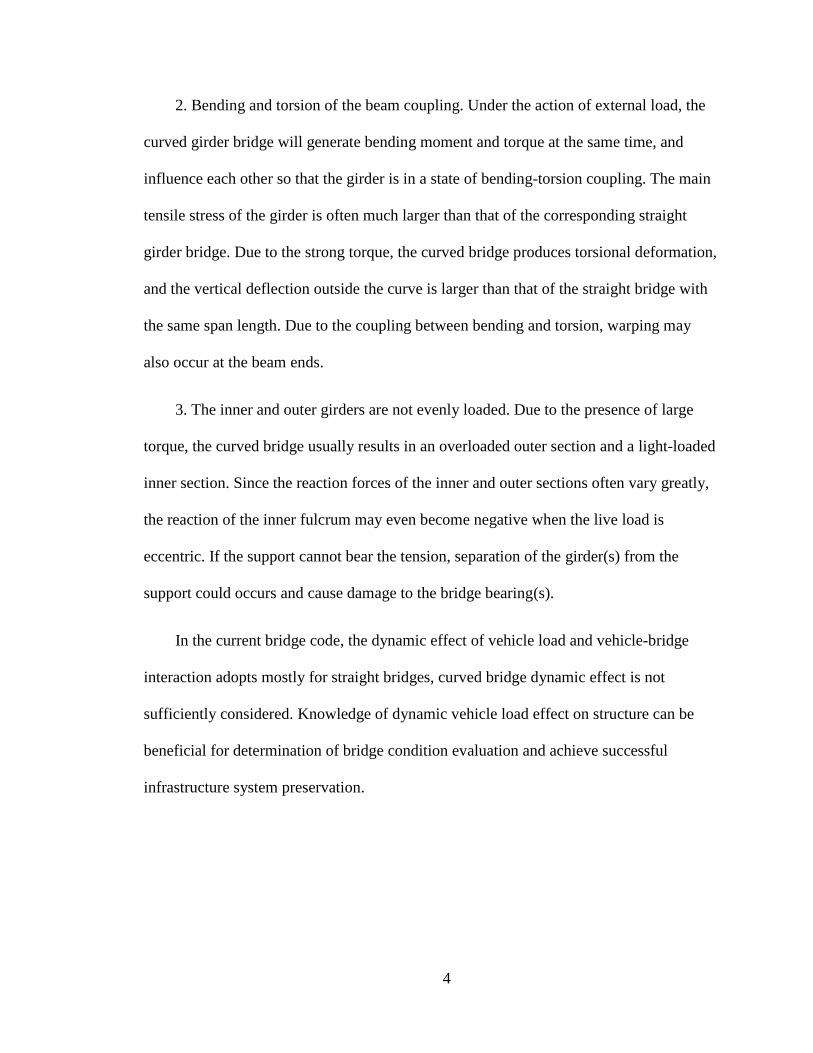
2. Bending and torsion of the beam coupling. Under the action of external load, the
curved girder bridge will generate bending moment and torque at the same time, and
influence each other so that the girder is in a state of bending-torsion coupling. The main
tensile stress of the girder is often much larger than that of the corresponding straight
girder bridge. Due to the strong torque, the curved bridge produces torsional deformation,
and the vertical deflection outside the curve is larger than that of the straight bridge with
the same span length. Due to the coupling between bending and torsion, warping may
also occur at the beam ends.
3. The inner and outer girders are not evenly loaded. Due to the presence of large
torque, the curved bridge usually results in an overloaded outer section and a light-loaded
inner section. Since the reaction forces of the inner and outer sections often vary greatly,
the reaction of the inner fulcrum may even become negative when the live load is
eccentric. If the support cannot bear the tension, separation of the girder(s) from the
support could occurs and cause damage to the bridge bearing(s).
In the current bridge code, the dynamic effect of vehicle load and vehicle-bridge
interaction adopts mostly for straight bridges, curved bridge dynamic effect is not
sufficiently considered. Knowledge of dynamic vehicle load effect on structure can be
beneficial for determination of bridge condition evaluation and achieve successful
infrastructure system preservation.

5
1.3 Research objective
Although considerable deal of research has been done on the coupling vibration of
bridge, most of the previous researches focused on the research of the straight girder
bridge. Few studies have been done on the impact effect of curved bridges. Engineers do
not have full understanding of the influencing factors of vehicle bridge coupled vibration
of curved bridges, and further research is needed. Besides, the current impact factor for
traffic load on highway does not reflect the influence from the grade of bridge surface
roughness. However, surface roughness is proven by majority of researchers to have a
great impact on the vehicle dynamic load. Whether the bridge dynamic response can be
covered by a unified impact factor calculation formula, and whether the existing impact
factor formula can be directly applied to the curved bridge, such problems have no
answers yet. More theoretical studies are needed in order to provide a practical empirical
formula to improve the design theory of curved bridges and maintenance and retrofit
methods for existing curved bridges.
The specific objective of this research is to study the curved bridge dynamic
response under vehicle-bridge interaction. First, by using commercial program ANSYS,
several multi-beam models of an existing bridges were built based on shear force flexible
grillage method. The warping stiffness and moment of inertia are both considered in this
model. A spatial vehicle model with 24 degrees of freedoms (DOFs) with three-
dimensional beam element, mass element and spring-damper elements is adopted in the
model. Taking effect of random surface roughness, the separation iteration algorithm is

6
used to the coupled vibration of the two subsystems. Second, using the model proposed
above, this research analyzes the influence of vehicle speed, surface roughness, radius of
curvature, lane eccentricity, stiffness and damping of tires and bridge structure, in order
to fully understand the influence factors of dynamic response of curved bridges. Also, the
influence of multi-lane loading, vehicle number and vehicle spacing on the impact factor
is studied.

7
2. Literature review
2.1 Vehicle model
By treating the vehicle as a moving force or pulsating load and neglecting the
vehicle inertia effect, Timoshenko (1922) published considerable different approximate
solutions for the moving load over simple beam structure dynamic interaction problem
(Figure 2.1). Hu Ding et al. (2013) investigated the dynamic interaction problem with a
beam supported by nonlinear viscoelastic foundations. With this beam model, essential
dynamic characteristics of bridge under moving traffic can be observed with a reasonable
degree of accuracy. However, this method ignores the interaction between the bridges
and moving vehicle, therefore the moving load method is only available for cases where
the mass of the traffic is relatively small to the bridge. Since the moving force/load model
is the simplest model that can be applied to the interaction problem, this method has been
frequently adopted by researchers when dealing with the vehicle-bridge interaction
problem. Arshad Mehmood (2014) developed a method combines finite element method
and Newmark time integration method in vibration analysis. Using computer code written
in Matlab, the dynamic response of the structures and critical load velocities can be found
with high accuracy.

8
Figure 2-1 Moving load model
When the inertia of the vehicle should be taken into consideration, the moving mass
model (Figure 2.2) is the simplest model that can be adopted. The inertial effects of
bridge and the moving vehicle were studied as early as in 1929 by Jeffcott by the method
of successive approximations. The investigations along this line were later carried out by
many researchers. Ting (1974) and Sadiku (1987) developed the algorithms for moving
mass problem using Green’s function. Ichikawa and Miyakawa (2000) combine eigen-
function expansion or modal analysis method and the direct integration method to obtain
a simple solution for moving mass vibration analysis. Eftekhar Azam et al. (2012)
transformed the partial differential equations of the system into the Ordinary Differential
Equations and obtained a reasonable accuracy. One of the major drawbacks of the
moving mass solution is that it fails to introduce the behavior of the bouncing action of
the vehicle and the bridge. This so-called bouncing effect is usually considered to be
significant when poor surface condition is presented.

9
Figure 2-2 Moving mass model
By considering the elastic and damping effects of the suspension system, the vehicle
model can be further enhanced. One simplest model, in this case, is the sprung mass
model which is a moving mass supported by a spring unit (Figure 2.3). Since early 60s,
researchers such as Biggs (1964) presented a semi-analytical solution to the simple beam
sprung mass interaction problem. Pesterev (2001) studied the behavior of an elastic
continuum when under multiple moving oscillations using the series expansion
technique. Later on, he discovered that for a simply support beam under oscillator load
and moving mass problem, there is little difference in area of the beam displacements, but
the difference of the beam stresses is quite noticeable. Also, it was shown that for spring
with small stiffness, the moving oscillator problem is equivalent to the moving load
problem.

10
Figure 2-3 Sprung mass model
With the emergence of the high performance computers and computation software,
it becomes feasible to have a more realistic modeling of the dynamic properties of a
moving vehicle. The multiple-axle truck can be represented as a number of discrete
masses each support by a set of spring and dashpot (Figure 2.4). Yang (1999) created a
vehicle model as two sets of the spring dashpot unit supporting a rigid beam as vehicle
body, each set of spring support is modeled on top of a mass unit representing wheel. To
better represent the various dynamic properties of heavy trucks, vehicle models with
multiple degrees of freedom have been devised and used by Chu (1986), Wang (1991)
and Zhang (2001). Zhang introduced a classic 11 degrees-of-freedom model for the three
axle tractor-trailer HS20-44 truck, the truck is modeled as a nonlinear vehicle model with
five sprung masses. Such model is widely modified and applied in other researchers’
study. Mario Fafard (1996) proposed a sophisticated tractor and semi-trailer combination
model with 18 DOFs to describe its movement, the vertical displacement, pitching and
transverse rotations are accounted and assume to remain small throughout the analysis.
Although the use of a more sophisticated vehicle model can make the simulation more

11
realistic, it does cause certain computation problems, where divergence and slow
convergence may occur in the process of iteration.
Figure 2-4 Multiple-axle truck model
2.2 Bridge model
Beam model with simply-supported at both ends is the most well known structure
that has ever been adopted in the study of vehicle-bridge interactions. Usually, this model
is considered having no restriction on the type of structures involved in the vehicle-
interaction problems, since the structure can always be represented by finite elements of
various forms. This beam model has been adopt in past vehicle bridge interaction
researches on various types of bridges, such studies include multi-span bridge (Wu, Dai

12
1987; Marchesiello et al,. 1999), multi-girder bridge (Huang, Nowak, 1991), continuous
beams bridges (Yang, 1995) and curved girder bridges (Chang,1997; Yang, 2001).
One major concern in the simulation of the bridge response under vehicle load is the
influence of road surface roughness (Figure 2.5). It has been reported that road surface or
pavement roughness can significantly affect the impact response of bridges (Paultre,
1992).The surface profile depends primarily on the quality of the construction of road
pavement and the maintenance level after bridges enter service. In most cases, this three-
dimensional surface roughness is often approximated by random two-dimensional profile.
Gupta (1980) used a sine function to represent road surface roughness. The roughness
profile can be created using stationary Gaussian random process and specific power
spectral density functions to describe the randomness property of the bridge deck. Similar
methods were widely adopted by researchers in this area (Huang and Nowak, 1991;
Chang and Lee, 1994). The power spectral density functions developed by Dodds and
Robson (1973) has been modified and used by Wang and Huang (1992) in their analyses.
Marcondes and Burgess (1991) generated three different categories of the pavement by
using the data collected from field measurement.

13
Figure 2-5 vehicle bridge interaction with surface roughness model
2.3 Influence of horizontal curvature
The majority of early vehicle –induced vibration studies were focus on straight
beams scenarios. The horizontal moving load can be regarded as the centrifugal forces
created by the interaction force between curved bridge lane and moving vehicle. This
horizontal centrifugal force is usually constantly changing, contrary to the vertical
moving loads, which always stay at the same direction and received less impact from
vehicle traveling status such as speed. Pioneer researchers such as Tan and Shore (1968)
conducted research on vertical or out-of-plane vibration of curved girder interaction.
However, the in plane vibration of centrifugal focus acting on a curved girder was rarely
studied.
2.4 Method of Solution
Two sets of equations of motion can be written in a vehicle-bridge interaction
system, one for the bridge and the other for the vehicle. The two sets of equations are

14
considered coupled due to the contact (interaction) forces existing at the contact points
which also physically connecting these two subsystems (vehicle system and bridge
system). The system matrices are time-dependent due to moving contact points, therefore
the matrices must be updated and factorized at each time step. To solve these equations,
one method (Huang and Nowak, 1991) is assuming a set of initial values of
displacements of these subsystems’ contact points to start the analysis, the initial
interaction forces from vehicle can be solved as the model starting status. Next, the more
precise values of contact points displacements can be calculated by updating the bridge
integration equation with the contact forces from last step. This method can generate both
vehicles and bridge responses at any instant simultaneously. However, for studies
involving bridge cases that require more realistic and complex environment, such as high
volume traffic, different driving pattern and multiple surface conditions, the convergence
rate of such iteration could be low. To increase the convergence rate and calculation
efficient, later research develop a condensation method for model elements. Such
condensation procedure is widely accepted and considered as one of more efficient
approaches for solving the vehicle-bridge interaction problem. Yang and Lin (1995) used
the dynamic condensation method to eliminate the degrees of freedom associated with
each vehicle on the element level. Other methods that have been employed in solving the
equations of motion in the vehicle-bridge interaction problem include:
1. Direct integration methods (Newmark method 1959) and fourth-order Runge-
Kutta method (Chu, 1986);

15
2. Modal superposition method (Blejwas, 1979) along with various integration
schemes;
3. Fourier transformation method (Green and Cebon, 1994; Chang and Lee, 1994).
A more versatile approach was developed by Yang and Wu (2001), in this method
the vehicle equations are discretized in time domain. For each time step, Yang considered
the vehicle contact forces as a set of external loads and transformed as nodal loads matrix
to apply to bridge subsystem. In such way, the coupled subsystems’ behavior such as
bridge displacements, vehicle status for next time step can be solved. For the curved
bridge vehicle interaction where vertical and horizontal contract forces are both involved,
this procedure has been demonstrated to be quite flexible.
2.5 Damping influence
Damping refers to the consumption of energy in the process of structural vibration,
which is the fundamental parameter of structural dynamic analysis. The damping
performance has an important influence on the dynamic response of the structure.
Currently, most researchers have studied the influence of damping on the seismic
response of the building structure and bridge structure. The influence in the vehicle-
bridge interaction problem is less studied. The previous researchers focused on the
following two issues: (1) the selection method of damping value and damping parameter;
(2) the influence of damping value on the seismic response. The existing research results

16
show that damping can effectively dissipate the seismic energy and reduce the seismic
response of the structure. Y.F Song and S.H He (2001) analyzed the impact coefficient of
the bridge by taking the damping ratio as 0.02 and 0.05 respectively and pointed out that
the damping ratio has a great influence on the impact coefficient of the bridge, especially
at high speeds and lousy pavement conditions. Research from M. Maijka (2008) shows
that vehicle speed, axle system frequency, mass-span ratio, and bridge structure damping
have a significant influence on the dynamic response of the bridge, while the influence of
vehicle damping on the bridge response is almost negligible.
2.6 Impact factor
In practice, the dynamic response of a bridge is usually considered ideally by
introducing an impact factor during the calculation, the actual interaction force is taken as
the static load multiplied by this impact factor. This impact factor is defined as the ratio
of the maximum bridge dynamic response to the maximum bridge static response under
certain load situation and then minus one. One typical definition for the impact factor I is:
𝐼 =𝑅𝑑(𝑥)−𝑅𝑠(𝑥)
𝑅𝑠(𝑥) (2.1)
where 𝑅𝑑(𝑥) and 𝑅𝑠(𝑥) represent the maximum dynamic and static responses of the
bridge at the cross section 𝑥 of the bridge.

17
It is well known that serval variables could affect the impact factor of a bridge under
the excitation of moving vehicle, such as vehicle dynamic properties, vehicle speed and
pavement roughness. The bridge code, American Association of State Highway and
Transportation Officials (AASHTO) Standard Specification (2014 edition), used to relate
the impact factor to the bridge span length L, the impact factor I is defined as the
increment of the static response of the vehicle load and can be determined by the
formula:
𝐼 =50
𝐿+125≤ 0.3 (2.2)
However, in the AASHTO LRFD Bridge Design Specifications (2017), dynamic
load allowance is not a function of span length, and its value depends only on the
component and the limit state. AASHTO currently assigns values to dynamic load
allowance as following:
Table 2-1 Dynamic load allowance in AASHTO LRFD Bridge Design
Specification
Limit State Dynamic Load
Deck Joints: All Limit States 75%
All Other Components: Fatigue and Fracture Limit State 15%
All Other Components: All Other Limit States 33%
In codes from other countries, such as Canada and Australia, the dynamic behavior
is considered related to the fundamental frequency of the bridge. Canadian Ontario

18
Bridge Design Code (OHBDC-1983) introduced dynamic load allowance in the vehicle
bridge interaction, the allowance is specified as a function of the natural frequency of
vibration of the bridge. However, later field study indicates the field measurements have
a considerable scatter of values.
Figure 2-6 Dynamic load allowance in OHBDC
For curved bridge impact factor, Koichi (1985) field test on 21 curved bridges and
came up with equation for impact factor I:
1 + 𝐼 =𝑅𝑠
𝑅𝑝
5
𝐿≤ 1.4 (2.3)
where 𝑅𝑠 is the radius of curvature at the shear center of the curved bridge (m), 𝑅𝑝 is
the radius of curvature of the point of loading (m), L is the span of curved bridge. His
research also pointed out that impact factors generated by irregular loads are generally
smaller than those of continuously loads, and the outer girders tend to have larger impact
factors than those of inner girders.

19

20
3. Research Outline
Chapter 1 Introduction
The chapter illustrates the background, motivations, objectives and limitations of the
research.
Chapter 2 Literature Review
The chapter reviews the previous research work on vehicle bridge interaction
analysis, modeling method. The review lays the foundations and start point of the
research.
Chapter 3 Vehicle bridge interaction model
The chapter describes the basic theory of the vehicle and bridge structure model
that is going to be used in the research.
Chapter 4 Vehicle bridge interaction analysis using simple beam model, grillage
model and multi-beam grillage model
Two selected bridges, concrete and steel curved bridges, were modeled
using triple-beam model.
Chapter 5 Vehicle bridge interaction analysis using three-dimensional solid FEM
model
Model the selected bridge using three-dimensional solid FEM model for
comparison.

21
Chapter 6 and 7 Parametric Study
A parameter study is performed in order to quantify the effects of different
parameters on vehicle bridge dynamic interaction, including curvature radius, span
configurations, bridge pavement condition, lane location, vehicle properties and traveling
speed.
Chapter 8 Calculation of impact factor based on empirical functions
A simplified empirical function is summarized from previous parametric data. The
function is also compared to current method of determining impact factor. Comments and
suggestions are made.

22
4. Theory of Vehicle-Bridge Analysis
4.1 Dynamic Analysis Model and Dynamic Characteristic Parameter
Analysis of Curved Girder Bridge
For curved bridges, the principal axis of cross section of the girder beam and the
applied load are generally not in the same plane, which will cause vibration in three
dimensions. Therefore spatial beam element with six degrees of freedom for each node is
required to model the structure.
The x-axis is the axial direction of the unit, and the y-axis and z-axis are the main
axes of inertia of the section respectively. The displacements of the i and j nodes of the
unit are denoted as
𝛿𝑖 = [𝑢𝑖 𝑣𝑖 𝑤𝑖 𝜃𝑥𝑖 𝜃𝑦𝑖 𝜃𝑧𝑖]𝑇
𝛿𝑗 = [𝑢𝑗 𝑣𝑗 𝑤𝑗 𝜃𝑥𝑗 𝜃𝑦𝑗 𝜃𝑧𝑗]𝑇 (4.1)
The element displacement matrix as
𝛿𝑒 = [𝑢𝑖 𝑣𝑖 𝑤𝑖 𝜃𝑥𝑖 𝜃𝑦𝑖 𝜃𝑧𝑖 𝑢𝑗 𝑣𝑗 𝑤𝑗 𝜃𝑥𝑗 𝜃𝑦𝑗 𝜃𝑧𝑗]𝑇 (4.2)
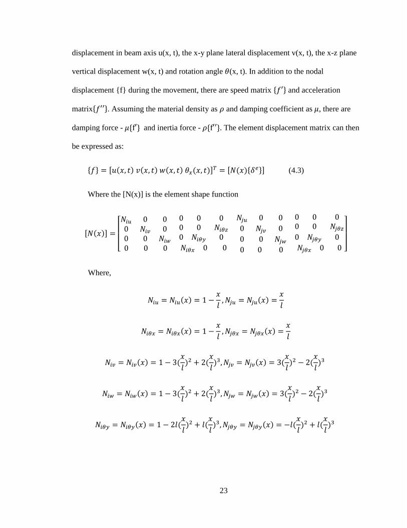
For a common curved girder in bridge engineering, the displacement and
deformation of the bridge can be described by four basic displacements: longitudinal
23
displacement in beam axis u(x, t), the x-y plane lateral displacement v(x, t), the x-z plane
vertical displacement w(x, t) and rotation angle 𝜃(x, t). In addition to the nodal
displacement f during the movement, there are speed matrix 𝑓′ and acceleration
matrix𝑓′′. Assuming the material density as 𝜌 and damping coefficient as 𝜇, there are
damping force - 𝜇f′ and inertia force - 𝜌f′′. The element displacement matrix can then
be expressed as:
𝑓 = [𝑢(𝑥, 𝑡) 𝑣(𝑥, 𝑡) 𝑤(𝑥, 𝑡) 𝜃𝑥(𝑥, 𝑡)]𝑇 = [𝑁(𝑥)𝛿𝑒] (4.3)
Where the [N(x)] is the element shape function
[𝑁(𝑥)] =
[ 𝑁𝑖𝑢 0 0
0 𝑁𝑖𝑣 00 0 𝑁𝑖𝑤
0 0 0
0 0 00 0 𝑁𝑖𝜃𝑧
0 𝑁𝑖𝜃𝑦 0
𝑁𝑖𝜃𝑥 0 0
𝑁𝑗𝑢 0 0
0 𝑁𝑗𝑣 0
0 0 𝑁𝑗𝑤
0 0 0
0 0 00 0 𝑁𝑗𝜃𝑧
0 𝑁𝑗𝜃𝑦 0
𝑁𝑗𝜃𝑥 0 0 ]
Where,
𝑁𝑖𝑢 = 𝑁𝑖𝑢(𝑥) = 1 −𝑥
𝑙, 𝑁𝑗𝑢 = 𝑁𝑗𝑢(𝑥) =
𝑥
𝑙
𝑁𝑖𝜃𝑥 = 𝑁𝑖𝜃𝑥(𝑥) = 1 −𝑥
𝑙, 𝑁𝑗𝜃𝑥 = 𝑁𝑗𝜃𝑥(𝑥) =
𝑥
𝑙
𝑁𝑖𝑣 = 𝑁𝑖𝑣(𝑥) = 1 − 3(𝑥
𝑙)2 + 2(
𝑥
𝑙)3, 𝑁𝑗𝑣 = 𝑁𝑗𝑣(𝑥) = 3(
𝑥
𝑙)2 − 2(
𝑥
𝑙)3
𝑁𝑖𝑤 = 𝑁𝑖𝑤(𝑥) = 1 − 3(𝑥
𝑙)2 + 2(
𝑥
𝑙)3, 𝑁𝑗𝑤 = 𝑁𝑗𝑤(𝑥) = 3(
𝑥
𝑙)2 − 2(
𝑥
𝑙)3
𝑁𝑖𝜃𝑦 = 𝑁𝑖𝜃𝑦(𝑥) = 1 − 2𝑙(𝑥
𝑙)2 + 𝑙(
𝑥
𝑙)3, 𝑁𝑗𝜃𝑦 = 𝑁𝑗𝜃𝑦(𝑥) = −𝑙(
𝑥
𝑙)2 + 𝑙(
𝑥
𝑙)3

24
𝑁𝑖𝜃𝑧 = 𝑁𝑖𝜃𝑧(𝑥) = 1 − 2𝑙(𝑥
𝑙)2 + 𝑙(
𝑥
𝑙)3, 𝑁𝑗𝜃𝑧 = 𝑁𝑗𝜃𝑧(𝑥) = −𝑙(
𝑥
𝑙)2 + 𝑙(
𝑥
𝑙)3
The speed and acceleration matrix can then be expressed as,
𝑓′ = [𝑢′(𝑥, 𝑡) 𝑣′(𝑥, 𝑡) 𝑤′(𝑥, 𝑡) 𝜃′(𝑥, 𝑡)]𝑇 = [𝑁(𝑥)]𝛿′𝑒 (4.4)
𝑓′′ = [𝑢′′(𝑥, 𝑡) 𝑣′′(𝑥, 𝑡) 𝑤′′(𝑥, 𝑡) 𝜃′′(𝑥, 𝑡)]𝑇 = [𝑁(𝑥)]𝛿′′𝑒 (4.5)
For element nodal load can be expressed as,
𝐹µ𝑒 = −∫[𝑁(𝑥)]𝑇 𝜇f ′dV
𝐹𝜌𝑒 = −∫[𝑁(𝑥)]𝑇 𝜌f′′ dV (4.6)
Which can also be expressed as,
𝐹µ𝑒 = −∫[𝑁(𝑥)]𝑇 𝜇𝑁(𝑥)𝛿′𝑒dV = −[𝑐𝑒]𝛿′𝑒
𝐹𝜌𝑒 = −∫[𝑁(𝑥)]𝑇 𝜌𝑁(𝑥)𝛿′′𝑒dV = −[𝑚𝑒]𝛿′′𝑒 (4.7)
Where
[𝑐𝑒] = ∫[𝑁(𝑥)]𝑇 𝜇𝑁(𝑥)dV
[𝑚𝑒] = ∫[𝑁(𝑥)]𝑇 𝜌𝑁(𝑥)dV
Assuming that the unit force is been applied nodal load 𝑃𝑒, the element
equilibrium equation can be written as

25
[𝑚𝑒]𝛿′′𝑒 + [𝑐𝑒]𝛿′𝑒 + [𝑘𝑒]𝛿𝑒 = 𝑃𝑒 (4.8)
And the global equilibrium equation
[𝑀]𝛿′′ + [𝐶]𝛿′ + [𝐾]𝛿 = [𝑃] (4.9)
Without any damping effect, an undamped free vibration equation of the structure
can be obtained
[𝑀]𝛿′′ + [𝐾]𝛿 = [0] (4.10)
Assume this free vibration is simple harmonic vibration
[𝛿(𝑡)] = [𝜑]sin (𝜔𝑡 + 𝜃)
[𝐾] − 𝜔2[𝑀][𝜑] = [0]
According to the Cramer’s rule, to obtain a nontrivial solution to a homogeneous
linear system of equations, the coefficient determinant mush equal to zero. In this case, it
is
[𝐾] − 𝜔2[𝑀] = [0] (4.11)
This equation is called the frequency equations of the system. For an equation of a
N-degree-of-freedom system will have N roots of the equation representing the
frequencies of the N possible modes of the system. These N frequencies arranged in the
order from small to large will constitute the spectrum of the system. The smallest
frequency is the fundamental frequency of the structure and the fundamental mode

26
corresponding to the first vibration mode. Such eigenvalue problems are usually solved
by matrix iterative method, this research use Block Lanczos method.
4.2 Multi-axis vehicle model description
4.2.1 Vehicle model coordinate systems
In order to describe the dynamics of vehicles moving on curved bridges, three sets
of coordinate systems are introduced, the fixed ground coordinate system, the vehicle
coordinate system and the wheel coordinate system.
Fixed ground coordinate system
To describe the steering attitude and trajectory of the vehicle, Cartesian coordinate
system fixed on the ground (X, Y, Z) is selected as the reference frame. For convenience,
the origin of the fixed ground coordinate system is set at the center of the curvature and
the driving trajectory of the vehicle is described as a cylindrical-coordinate system.
Vehicle coordinate system
The vehicle coordinate system (x, y, z) is a coordinate system that is fixed on the
vehicle with the vehicle mass center (MC) as the origin and moves with the vehicle. The
vehicle motion parameters according to the right-handed Cartesian coordinate define the
coordinate system as follows.
x – Forward, travelling direction of the vehicle

27
y – Pointing to the left side of the vehicle travelling direction
z – Pointing vertically upward from vehicle
𝜃𝑥 − The roll angle around the axis x
𝜃𝑦 − The pitch angle around the axis y
𝜃𝑧 − The yaw angle around the axis z.
Wheel coordinate system
The wheel coordinate system (𝑥𝑖 , 𝑦𝑖 , 𝑧𝑖) is a coordinate system that is fixed on the
wheel and moves with the wheel based on the axle center TC. The system is used to
describe the dynamic interaction force between the vehicle and the bridge and it is
defined by the right-handed Cartesian coordinated system as follows.
𝑥𝑖 – Forward, on the longitudinal plane of symmetry of the wheel
𝑦𝑖 – Point to the left along the axle in the wheel rolling direction
𝑧𝑖 – Point upward in the vertical direction from the wheel
𝛿𝐿– The attack angle of the steering wheel around the axis, called the Ackermann
steering angle, which is used to describe the kinematic effect of a vehicle’s steady-state
steering.
4.2.2 Simplified vehicle model (3-axle)
In this study, the typical 3-axle vehicle is simplified into a vibration system
connected by mass, spring and damper. The body is modeled as a rigid body, and the

28
suspension system and tire are modeled jointly by a spring and a viscous damper with
energy dissipation capability. The mass of the suspension system and tire is simulated by
the ideal mass elements. The model considers the vertical and horizontal vibrations of the
vehicle and the rotational vibration around the three axes. The simplified model of the
vehicle is shown in the figure below. The model contains a total of 12 generalized
degrees of freedom. Among them, four generalized coordinates of 𝑦𝑚, 𝑧𝑚, 𝜃𝑥𝑚, 𝜃𝑦𝑚 are
selected to describe the lateral vibration, vertical vibration, roll around the x axis and
pitch vibration around the y axis. Coordinates 𝑧1, 𝑧′1, 𝑦1 from front suspension are
selected to describe the vertical vibration, lateral vibration, five generalized coordinates
from rear suspension 𝑧2, 𝑧′2, 𝑧3, 𝑧′3, 𝑦1, 𝑦2 are used to describe its vertical vibration,
Lateral vibration, rolling, and pitching vibration, respectively.
Figure 4-1 3-axle truck model and degrees of freedom

29
Figure 4-2 3-axle truck model and degrees of freedom
4.2.3 Simplified vehicle model (3D, 3-axle)
In this study, an improved 3D vehicle model which is based on the typical 2D
model, is introduced in the later analysis. Vehicle is considered as two connected ‘half
truck’ models. Additional pseudo beam is also modeled in the bridge model to support
the 3D vehicle model and distribute the interaction forces. By applying the elevation
differentials of the support beam, the influence of the curved bridge horizontal elevation
in the vehicle bridge interaction can be studied.
Figure 4-3 3D truck model

30
4.3 Random surface roughness
It is assumed that the roughness of the pavement is a Gaussian random process with
power spectrum to represent the statistical characteristics of the pavement. In this study,
analysis chooses method developed by Eui-Seung Hwang and Wewak (1990),
𝑆𝑟(Ω) = 𝛼Ω𝑘−𝛽
Ω𝐿 < Ω𝐾 < Ω𝑈
0 𝑜𝑡ℎ𝑒𝑟𝑤𝑖𝑠𝑒 (4.12)
Where
β – Frequency factor, 0.2
α – Surface roughness ratios
Ω – Spatial frequency, the inverse of the wavelength, indicating the number of
occurrences of a harmonic in each meter.
Ω𝐿 Ω𝑈 – Lower and upper limits of the spatial frequency
After applying inverse fast Fourier transform to above formula, the vertical
distribution function of the vertical irregular shape of the bridge deck can be obtained.
𝑟(𝑠) = ∑ 𝛼𝐾𝑁𝐾=1 𝐶𝑂𝑆(2𝜋Ω𝑘 𝑠 + 𝜙𝑘) (4.13)
Where
𝛼𝐾 – Amplitude
𝜙𝑘- Random phase angle, random numbers between [0, 2𝜋];
s - Longitudinal coordinates of the bridge.

31
4.4 Vehicle-Bridge coupling analysis
4.4.1 Basic assumptions
In current study, the models used for vehicle bridge interaction analysis follow these
assumptions.
1. When a vehicle travels along the curved bridge, the instantaneous center of
rotation coincides with the center of curvature of the circular curve, and the deflection
angle of the inner steering wheel is greater than the deflection angle of the outer steering
wheel.
2. The vehicle lateral slip angle of the center of mass does not change with time and
the vehicle makes a steady circular motion on the circumference. Also, the attack angle of
the vehicle front wheel remains constant.
3. This study ignores the elastic deformation of the vehicle body, the suspension and
axle. The vehicle body, suspension and axle are treated as rigid bodies where they are
connected by springs and dampers. Dampers are assumed to have linear viscous damping
property.
4. The body, the suspension and each pair of rigid bodies of the wheelset make small
displacement vibration at the balance position, and does not consider the influence of the
change of the vehicle center of gravity height on the centrifugal force and the centrifugal
moment caused by the slight vibration generated by the vehicle body under the
unevenness of the bridge deck.

32
Figure 4-4 Centrifugal forces on the moving vehicle
5. The vehicle model is symmetrical along the longitudinal direction; the model
ignores the vibration along the longitudinal axis. The rear wheels are travelling on the
ruts of the front wheels.
4.4.2 Motion equations of vehicle
Based on the commercial finite element analysis software ANSYS, the spring-
damping element, mass element and the rigid rod space rod element are used to simulate
the components of the vehicle. The vehicle model is discretely modeled according to the
finite element method. The vibration equation of the vehicle can be expressed as.
𝑚𝑣𝑧′′ + 𝑐𝑣𝑧′ + 𝑘𝑣𝑧 = 𝑓𝑣 (4.14)
Where 𝑚𝑣, 𝑐𝑣, 𝑘𝑣 and 𝑓𝑣 represent vehicle mass matrix, damping matrix, stiffness
matrix and outside external excitation vector, respectively.

33
4.4.3 Motion equations of bridge
The bridge model is discretized by the finite element method, and the equation of
motion of bridge is,
[𝑀𝑏]𝛿′′ + [𝐶𝑏]𝛿
′ + [𝐾𝑏]𝛿 = [𝑃𝑏] (4.15)
Where [𝑀𝑏], [𝐶𝑏], [𝐾𝑏] represent global mass matrix, global damping matrix and
global stiffness matrix of the bridge structure, respectively. [𝑃𝑏] is the external load
vector, which is resulting from the vehicle bridge interaction. To simplify the global
damping matrix, the [𝐶𝑏] is usually taken as
[𝐶𝑏] = 𝛼[𝑀𝑏] + 𝛽[𝐾𝑏] (4.16)
The factors 𝛼 and 𝛽 can be obtained by,
𝛼 = (2𝜔1 𝜔2 (𝜉1𝜔2 − 𝜉2𝜔1))/(𝜔22 − 𝜔1
2)
𝛽 =2(𝜉2𝜔2−𝜉1𝜔1)
𝜔22−𝜔1
2 (4.17)
Where 𝜔1, 𝜔2 are free vibration frequencies of two selected mode shapes, and 𝜉1 , 𝜉2
are their respective damping ratios.
4.4.4 Solution of vehicle bridge dynamic interaction force
The forces acting on the bridge by a vehicle traveling on a curved girder bridge
include the following two factors. First, vertical and lateral wheel loads due to centrifugal

34
forces, and second, dynamic loads caused by vehicle self-weight and bridge deck
roughness excitation.
4.4.5 Centrifugal force effect
When a vehicle travelling in a uniform circular motion, centrifugal force 𝑚𝑣𝑣2/𝜌
and moment 𝑚𝑣𝑣2ℎ/𝜌 will apply to the mass center of the vehicle. During the circular
motion, the mass center will have a lateral displacement ℎ 𝑠𝑖𝑛𝑥 (hx). The total moment
can be expressed as.
𝑀 =𝑚𝑣𝑣
2ℎ
𝜌+ 𝑚𝑣𝑔ℎ𝑥 (4.18)
Assume the distances between vehicle mass center to the front and rear suspension
centers to be 𝑙𝑉, 𝑙𝐻. The centrifugal forces for front and rear suspensions would be
𝑚𝑣𝑣2𝑙𝑣/(𝜌𝑙) and 𝑚𝑣𝑣
2𝑙𝐻/(𝜌𝑙).
Assume the rolling angular stiffness for front and rear axles are 𝐶𝑉 , 𝐶𝐻. The total
moment can also be expressed as.
𝑀 = (𝐶𝑉 + 𝐶𝐻)𝑥 (4.19)
The rolling angle can then be expressed as.
𝑥 =𝑚𝑣(
𝑣2
𝜌)ℎ
𝐶𝑉+𝐶𝐻−𝑚𝑣𝑔ℎ (4.20)
And the spring moment for both axles.

35
𝑀𝐹𝑉 = 𝐶𝑉𝑥 =𝐶𝑣𝑚𝑣𝑔ℎ
𝐶𝑉 + 𝐶𝐻 − 𝑚𝑣𝑔ℎ
𝑣2
𝜌𝑔
𝑀𝐹𝐻 = 𝐶𝐻𝑥 =𝐶𝐻𝑚𝑣𝑔ℎ
𝐶𝑉+𝐶𝐻−𝑚𝑣𝑔ℎ
𝑣2
𝜌𝑔 (4.21)
The load differential of front and rear axle is.
∆𝐹𝑧1𝑠1 = 𝑀𝐹𝑉 +𝑚𝑣𝑣
2𝑙𝐻𝑝𝑉
𝜌𝑙+ 𝑚1𝑣
2ℎ𝑣/𝜌
∆𝐹𝑧𝐻𝑠𝐻 = 𝑀𝐹𝐻 +𝑚𝑣𝑣
2𝑙𝑉𝑝𝐻
𝜌𝑙+ 𝑚2𝑣
2ℎ𝐻/𝜌 (4.22)
Where the rear axle ∆𝐹𝑧𝐻 = ∆𝐹𝑧2 + ∆𝐹𝑧3 = 2∆𝐹𝑧2 = 2∆𝐹𝑧3, 𝑝𝐻, 𝑝𝑣 are the
horizontal and vertical distances of the suspension center to road surface, ℎ𝐻 , ℎ𝑣 are the
horizontal and vertical distances of axle mass center to road surface.
By combining the equations above, the differences between dynamic and static
wheel loads are.
∆𝐹𝑧1 = 𝑚𝑣𝑣2/𝜌(
𝐶𝑉
𝐶𝑉 + 𝐶𝐻 − 𝑚𝑣𝑔ℎ
ℎ
𝑠1+
𝑙𝐻𝑙
𝑝𝑉
𝑠1+
𝑚1
𝑚𝑣
ℎ𝑣
𝑠1)
∆𝐹𝑧2 = ∆𝐹𝑧3 = 𝑚𝑣𝑣2/𝜌(
𝐶𝐻
𝐶𝑉+𝐶𝐻−𝑚𝑣𝑔ℎ
ℎ
𝑠2+
𝑙𝑉
𝑙
𝑝𝐻
𝑠2+
𝑚2
𝑚𝑣
ℎ𝐻
𝑠1) (4.23)
4.4.6 Bridge deck roughness effect
Assuming that the wheels and the deck are always in contact with each other
when the vehicle runs through the bridge, the wheel and bridge contact points can be used

36
to generate the dynamic load of the bridge. The dynamic loading between wheels and
bridge can be written as.
𝐹𝑑𝑖𝑗 = 𝑐𝑡𝑖𝑗 [𝑧′𝑠𝑖𝑗 − 𝜁′
𝑡𝑖𝑗(𝑠, 𝑡) − 𝑟′(𝑠𝑖𝑗)] + 𝑘𝑡𝑖𝑗[𝑧𝑠𝑖𝑗 − 𝜁𝑡𝑖𝑗(𝑠, 𝑡) − 𝑟(𝑠𝑖𝑗)] (4.24)
Where
i = L, R represents left or right side of vehicle
j = 1,2,3 represents the axle number
𝜁𝑡𝑖𝑗(𝑠, 𝑡) represents the bridge displacement at given time and location
𝑟(𝑠𝑖𝑗) represents the roughness at given location
The external excitation due to surface roughness can then be expressed as.
𝑓𝑣𝑖𝑗 = 𝑐𝑡𝑖𝑗 [𝜕𝜁𝑡𝑖𝑗(𝑠,𝑡)
𝜕𝑡+ 𝑣
𝜕𝑟(𝑠)
𝜕𝑠] + 𝑘𝑡𝑖𝑗[𝜁𝑡𝑖𝑗(𝑠, 𝑡) + 𝑟(𝑠)] (4.25)

37
5. Vehicle bridge interaction analysis and preliminary result
5.1 Case study bridge models
To study the vehicle-bridge dynamic analysis, two typical curved bridges,
Manchuria concrete bridge in China and Veteran’s Memorial steel bridge in Florida,
United States, were selected to be modeled in ANSYS. Three different models, a simple
beam model, a grid model and a three-dimensional solid element model, were built and
analyzed.
5.1.1 Manchuria Interchange Bridge
Manchuria Interchange is a cross-over bridge on the HaiMan Highway, built in 2007
with a bridge deck width of 12m, carriageway of 11m and a 6% cross-slope. The
superstructure adopts prestressed concrete continuous curved box girder with a curve
radius of 280m. The main girder is a single-box double-chamber section with a beam
height of 1.90m. The whole structure is a consolidation of pier and beam rigid frame
system. The lower structure is a ribbed platform, the foundation of the pier is a rock-fill
pile foundation, and the abutment adopts a basin rubber bearing as shown in Figure 5.1.

38
Figure 5-1 Manchuria bridge layout and cross section
Table 5-1 Section properties of bridge model
Section property Girder Pier
Cross-section area A(𝑚2) 7.998~16.022 2.400
Vertical bending inertia 𝐼𝑦 (𝑚4) 4.047~5.808 0.288
Horizontal bending inertia 𝐼𝑧 (𝑚4) 86.720~114.700 0.800
Free torsional inertia 𝐼𝑑 (𝑚4) 9.627~14.681 0.721
Fixed torsional inertia 𝐼𝜔 (𝑚4) 12.178~17.488 0.022
According to the design drawings of the actual bridge, considering the influence of
the crash barriers on the dynamic characteristics of the structure, the simplified beam-
type and triple-beam grid dynamic analysis models were respectively established. The

39
properties of concrete in the model are as follows: Young's modulus𝐸𝑐 = 34.5𝐺𝑃𝑎,
Poisson's ratio 𝜐 = 0.20, mass density 𝜌 = 2500𝑘𝑔 / 𝑚3.
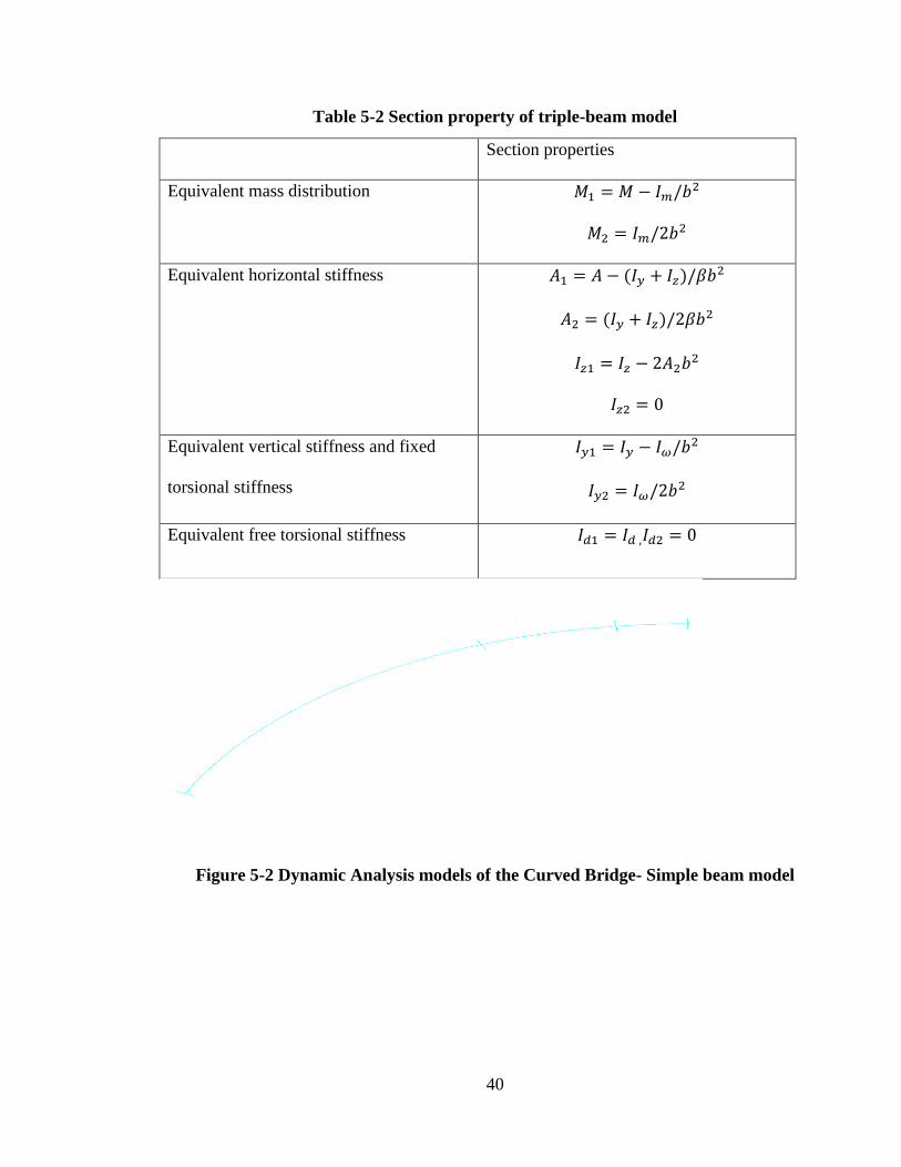
The three-beam dynamic analysis model reasonably distributes the mass and
stiffness of the deck system to the middle and two side beams according to a certain
equivalent method. Based on this, the mass distribution and cross-section characteristics
of each main beam in the model are determined. To represent the actual bridge, section
properties of the main girders in the triple-girder model are calculated by the formulas in
Table 5.2. The stiffness of the horizontal beam is related to the spacing 𝑏1 of the girder.
The horizontal beam is modeled by a massless element. The piers are fixed at the bottom
where both ends of the main beam only constrained the vertical displacement.
40
Table 5-2 Section property of triple-beam model
Section properties
Equivalent mass distribution 𝑀1 = 𝑀 − 𝐼𝑚/𝑏2
𝑀2 = 𝐼𝑚/2𝑏2
Equivalent horizontal stiffness 𝐴1 = 𝐴 − (𝐼𝑦 + 𝐼𝑧)/𝛽𝑏2
𝐴2 = (𝐼𝑦 + 𝐼𝑧)/2𝛽𝑏2
𝐼𝑧1 = 𝐼𝑧 − 2𝐴2𝑏2
𝐼𝑧2 = 0
Equivalent vertical stiffness and fixed
torsional stiffness
𝐼𝑦1 = 𝐼𝑦 − 𝐼𝜔/𝑏2
𝐼𝑦2 = 𝐼𝜔/2𝑏2
Equivalent free torsional stiffness 𝐼𝑑1 = 𝐼𝑑 ,𝐼𝑑2 = 0
Figure 5-2 Dynamic Analysis models of the Curved Bridge- Simple beam model

41
Figure 5-3 Dynamic Analysis models of the Curved Bridge- Triple-beam model
Figure 5-4 Dynamic Analysis models of the Curved Bridge- Solid finite element
model
Based on the bridge design and assumptions in Chapter 4, three types of model,
simple beam model, triple-beam model and finite element model, were built (Figure 5.2
to Figure 5.4). All three models have equivalent section properties. In the study, the
triple-beam model is focused.
1
MAY 17 2008
20:17:35
ELEMENTS

42
For triple-beam model, three typical HS20 truck models (two 2D models and one 3D
model) were built with spring-damper-mass elements as shown in Figure 5.5 to Figure
5.7.
Figure 5-5 Typical 2-axle truck models used in the vehicle-bridge
Figure 5-6 Typical 3-axle truck models used in the vehicle-bridge

43
Figure 5-7 Typical 3D 3-axle truck models used in the vehicle-bridge analysis
For 3D vehicle model, additional pesudo beam is created in the bridge model to
support the vehicle. By adjusting the bridge horizontal elevation, the influnence of
elevation in the curved bridge vehicle interaction is studied.
To study the influence of bridge surface roughness during vehicle-bridge interaction.
Using Matlab Three sets of roughness profiles representing different bridge deck
conditions are randomly generated and applied during the dynamic analysis. Good
surface condition (𝑎 = 0.18 × 10⁻⁶𝑚3/𝑐𝑖𝑟𝑐𝑙𝑒), normal surface condition (𝑎 =
2.5 × 10⁻⁶𝑚3/𝑐𝑖𝑟𝑐𝑙𝑒), poor surface condition (𝑎 = 10 × 10−6𝑚3/𝑐𝑖𝑟𝑐𝑙𝑒) are shown in
Figure 5.4a, b, and c, respectively. Additional profile of perfect surface condition
(smooth surface) is also modeled for comparison purpose.

44
Figure 5-8 Roughness profiles of different types of deck (Good surface
condition)
Figure 5-9 Roughness profiles of different types of deck (Normal surface
condition)
Figure 5-10 Roughness profiles of different types of deck (Bad surface
condition)
To reduce the effect of extreme values in the randomly generated surface conditions,
each class of roughness profile is respresented by three sets of surface condition profiles
using the same variables in the generating process. The mean values of model reactions
are selected in the study.

45
To study the influence of eccentric traffic during the dynamic interaction, three types
of eccentric conditions (e=-3.1m, e=0m, e=+3.1m) were also considered to simulate the
situation where trucks traveling in different lanes.
5.1.2 Veteran’s Memorial Bridge
As a second example, Veteran’s Memorial Bridge is a curved steel box girder bridge
carrying US-319 in Tallahassee, Florida. The same bridge is tested and analized before
by Huang(2002). It consists of two sections of three-span continuous girders; one section
is straight and the other is curved. The end spans of the curved box girder bridge are
50.54m long and the middle span is 75.80m long. The cross section is composed of two
built-up steel-box girders and composite with the deck. Top flange thickness varies from
2.22 to 6.99 cm and the bottom flange thickness varies from 1.27 to 3.18 cm. The deck is
20.32 cm thick and 13.31 m wide from outside to outside. Internal cross frames are
spaced at 3.08 m, except for the end spacing, which is 2.71 m. There is no external
bracing between box girders, except at sections over the supports (Figure 5.5).

46
Figure 5-11 Veteran’s bridge layout and cross section
Table 5-3 Section properties of bridge model
Section property Girder Pier
Cross-section area A(𝑚2) 5.4876 2.400
Vertical bending inertia 𝐼𝑦 (𝑚4) 3.699 0.288
Horizontal bending inertia 𝐼𝑧 (𝑚4) 77.2807 0.800
Free torsional inertia 𝐼𝑑 (𝑚4) 3.7185 0.721

47
Similar to the Manchuria bridge, a triple-beam model was constructed with typical
2-axle and 3-axle truck moving across the bridge with three different types of deck
surface conditions.
5.2 Preliminary case study results
5.2.1 Manchuria Concrete Curved Bridge
Figures 5.12 to Figure 5.19 shows the displacement and moment responses of the
bridge when vehicle travel across the bridge with different speeds. It can be noticed that
in good surface condition, the maximum bridge response and moment response remain
relatively the same, regardless of the vehicle travelling speed. However, as the traveling
speed increased, the response curves became unstable
Figure 5-12 Flange deflection of mid span (vehicle speed v=10m/s)
-1.4
-1.2
-1
-0.8
-0.6
-0.4
-0.2
0
0.2
0.4
0.6
0 20 40 60 80 100 120
3 axle, 10m/s, e=-3.1m, Good surface condition- Z displacement (mm) vs vehicle location (m)

48
Figure 5-13 Flange deflection of mid span (vehicle speed v=20m/s)
Figure 5-14 Flange deflection of mid span (vehicle speed v=30m/s)
-1.5
-1
-0.5
0
0.5
1
0 20 40 60 80 100 120
3 axle, 20m/s, e=-3.1m, Good surface condition- Z displacement (mm) vs vehicle location (m)
-2
-1.5
-1
-0.5
0
0.5
1
0 20 40 60 80 100 120
3 axle, 30m/s, e=-3.1m, Good surface condition- Z displacement (mm) vs vehicle location (m)

49
Figure 5-15 Flange deflection of mid span (vehicle speed v=40m/s)
Figure 5-16 Moment force response of mid span at v=10m/s
-1.5
-1
-0.5
0
0.5
1
0 20 40 60 80 100 120
3 axle, 40m/s, e=-3.1m, Good surface condition- Z displacement (mm) vs vehicle location (m)
-500
0
500
1000
1500
2000
2500
0 20 40 60 80 100 120
Mo
men
ts (
KN
.m)
Vehicle Position (m)
Member force response curves at the mid of the structure at 10m/s

50
Figure 5-17 Moment force response of mid span at v=20m/s
Figure 5-18 Moment force response of mid span at v=30m/s
-1000
-500
0
500
1000
1500
2000
0 20 40 60 80 100 120Mo
men
ts (
KN
.m)
Vehicle Position (m)
Member force response curves at the mid of the structure at 20m/s
-1000
-500
0
500
1000
1500
2000
2500
0 20 40 60 80 100 120
Member force response curves at the mid of the structure at 30m/s

51
Figure 5-19 Moment force response of mid span at v=40m/s
Figure 5.20 summarizes all amplification factors from the case study including
mid-span displacement, shear, moment, end-span displacement, shear and moment. As
shown in the figure, as the vehicle traveling speed increase, all the dynamic amplication
factors also increased slightly.
-1000
-500
0
500
1000
1500
2000
0 20 40 60 80 100 120
Member force response curves at the mid of the structure at 40m/s

52
Figure 5-20 Amplication factors of different traveling speeds.
Figure 5.21 to 5.25 shows bridge dynamic reaction when a 3-axle truck traveling at
outside good surface condition lane with the speed of 20m/s. By comparing displacement
charts from different surface condition, the influence of surface condition to bridge
dynamic response can be observed. Additional comparison is made between no surface
roughness (smooth surface) and ‘good condition’ surface. Noticed that as the surface
condition deteriorate, the impact of the truck on the bridge becomes larger, the vibration
of the structure is aggravated, and the amplitude of the dynamic response also gradually
increases.
0
0.5
1
1.5
2
2.5
3
3.5
0 20 40 60 80 100 120
Amplication factors vs. vehicle traveling speed (Good surface condition)
10m/s
16m/s
22m/s
30m/s
40m/s

53
Figure 5-21 Bridge girder deflection response of a 3-axle truck passing through
the bridge.
Figure 5-22 Bridge deflection response vs Good surface condition
-2
-1.5
-1
-0.5
0
0.5
1
3 axle, 20m/s, e=-3.1m, Good surface condition- Z displacement (mm) vs vehicle location (m)
-2
-1.5
-1
-0.5
0
0.5
1
0 20 40 60 80 100 120 140
Deflection of Good surface

54
Figure 5-23 Bridge deflection response vs Normal surface condition
Figure 5-24 Bridge deflection response vs Bad surface condition
-2
-1.5
-1
-0.5
0
0.5
1
0 20 40 60 80 100 120 140
Deflection of Normal surface
-3
-2.5
-2
-1.5
-1
-0.5
0
0.5
1
1.5
0 20 40 60 80 100 120 140
Deflection of Bad surface

55
Figure 5-25 Amplified factor vs different surface conditions
Figure 5.26 and 5.27 show the effect of deck roughness on the maximum absolute
displacement and dynamic amplification factor at the girder. It can be observed that when
the surface condition is ‘Good’, vehicle impact factor remains relative small regardless of
its travelling speed. With the deck condition deteriorates, the impact factor, as well as the
maximum absolute displacement starts to increase. The maximum impact factors increase
from 1.3 (Good condition) to 1.7 (Normal condition), while the maximum deflection
increase from 2.15mm (Good condition) to 2.7mm (Normal condition), roughly 26%
increment.
0
0.5
1
1.5
2
2.5
0 20 40 60 80 100 120
Amplified factor; good surface vs smooth surface
smooth surface good condition surface

56
Figure 5-26 Maximum deflections under different vehicle traveling speed and
road condition
Figure 5-27 Impact factor of bridge under different vehicle traveling speed and
road condition

57
Additional hypothetical straight bridge with the same Manchuria bridge properties is
modeled to observe the influence of curved bridge layout in the bridge vehicle
interaction. The detailed comparion are shown in Figure 5.28 to 5.30. Though the figures
show little differences in z-displacement and member force responses between these two
bridges, the impact factor comparison shows that the curved bridge has a noticable
increasment comparing to the straight one. It is reasonable to draw the conclusion that the
curved bridge layout have increased the vehicle bridge interaction.
Figure 5-28 Moment response comparison between curved Manchuria Bridge
and hypothetical straight Manchuria Bridge.
-1000
-500
0
500
1000
1500
2000
0 20 40 60 80 100 120
mo
men
t
vehicle location
member force response at the mid of structure v=30m/s curved bridge vs straight bridge
curved bridge
straight bridge

58
Figure 5-29 Z-displacements comparison between curved Manchuria Bridge
and hypothetical straight Manchuria Bridge.
Figure 5-30 Impact factor comparison between curved Manchuria Bridge and
hypothetical straight Manchuria Bridge.
-2
-1.5
-1
-0.5
0
0.5
1
0 20 40 60 80 100 120
z d
isp
lace
men
t
bridge location
2axle ev=0 v=30m/s, Good surface conditionZ displacement (mm) vs vehicle location
curved bridge
straight bridge
0
0.5
1
1.5
2
2.5
0 20 40 60 80 100 120
Imp
act
fact
or
bridge location (m)
Impact factor vs vehicle location [good surface condition v=30m/s]
curved bridge
straight bridge

59
5.2.2 Veteran’s Memorial Steel Curved Bridge
Figures 5.31 to 5.36 show the displacement and moment responses of the bridge
when vehicle travel through the bridge with different speeds. Compared to the Manchuria
concrete bridge, the bridge response is much higher. This is most likely due to the bridge
layout and materials. Also, as the vehicle speed increased, the maximum response of the
bridge slightly increased.
Figure 5-31 Girder deflection of mid span (vehicle speed v=28m/s)
-10
-8
-6
-4
-2
0
2
4
0 10 20 30 40 50 60 70 80 90
3 axle, 28m/s, e=-3.1m, Good surface condition- Z displacement (mm) vs vehicle location (m)
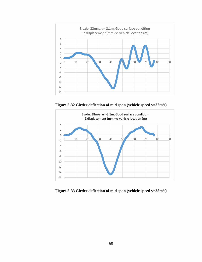
60
Figure 5-32 Girder deflection of mid span (vehicle speed v=32m/s)
Figure 5-33 Girder deflection of mid span (vehicle speed v=38m/s)
-14
-12
-10
-8
-6
-4
-2
0
2
4
6
8
0 10 20 30 40 50 60 70 80 90
3 axle, 32m/s, e=-3.1m, Good surface condition- Z displacement (mm) vs vehicle location (m)
-16
-14
-12
-10
-8
-6
-4
-2
0
2
4
0 10 20 30 40 50 60 70 80 90
3 axle, 38m/s, e=-3.1m, Good surface condition- Z displacement (mm) vs vehicle location (m)

61
Figure 5-34 Moment force response of mid span (vehicle speed v=28m/s)
Figure 5-35 Moment force response of mid span (vehicle speed v=32m/s)
-1000
-500
0
500
1000
1500
2000
2500
Member force response curves at the mid of the structure at 28m/s
-1000
-500
0
500
1000
1500
2000
2500
0 50 100 150 200
Member force response curves at the mid of the structure at 32m/s
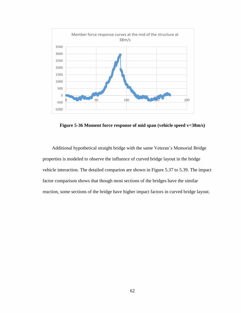
62
Figure 5-36 Moment force response of mid span (vehicle speed v=38m/s)
Additional hypothetical straight bridge with the same Veteran’s Memorial Bridge
properties is modeled to observe the influence of curved bridge layout in the bridge
vehicle interaction. The detailed comparion are shown in Figure 5.37 to 5.39. The impact
factor comparison shows that though most sections of the bridges have the similar
reaction, some sections of the bridge have higher impact factors in curved bridge layout.
-1000
-500
0
500
1000
1500
2000
2500
3000
3500
0 50 100 150 200
Member force response curves at the mid of the structure at 38m/s

63
Figure 5-37 Moment response comparison between curved Veteran’s Memorial
Bridge and hypothetical straight Veteran’s Memorial Bridge.
Figure 5-38 Z-displacements comparison between curved Veteran’s Memorial
Bridge and hypothetical straight Veteran’s Memorial Bridge.
-2000
-1000
0
1000
2000
3000
4000
5000
0 10 20 30 40 50 60 70 80 90
mo
men
t
vehicle location (m)
member force response at the mid of structure v=30m/s curved bridge vs straight bridge
curved bridge
straight bridge
-15
-10
-5
0
5
10
0 10 20 30 40 50 60 70 80 90
z d
isp
lace
men
t (m
m)
vehicle location (m)
3axle ev=0 v=30m/s, Good surface conditionZ displacement (mm) vs vehicle location
curved bridge
straight bridge

64
Figure 5-39 Impact factor comparison between curved Veteran’s Memorial
Bridge and hypothetical straight Veteran’s Memorial Bridge.
5.3 Preliminary case study summary
Comparison is made for the case study Manchuria concrete bridge and Memorial
steel bridge. By examining their bridge responses, it can be observed that the dynamic
interaction of a curved bridge could be greatly influence by various factors. As the
vehicle travelling speeds increase and surface conditions deteriorate, the bridge impact
factors increase considerably. Such behavior agrees with most previous researches
regarding vehicle bridge interaction. The hypothetical straight bridge models of both
cases show that the curvature also plays an important part in such dynamic interaction,
the curved models generally have a higher dynamic response than the straight versions. A
1
1.05
1.1
1.15
1.2
1.25
0 10 20 30 40 50 60 70 80 90
Imp
act
fact
or
bridge location (m)
Impact factor vs bridge location
curved bridge
straight bridge

65
detail parametric study is required to understanding how each factor contribute in the
vehicle bridge interaction problem.

66
6. Parametric Study
6.1 Introduction
The vehicle bridge interaction has discussed in two different bridges from previous
chapter. The object of this chapter is to expand the previous obtained results to a wider
range of curved bridges in order to evaluate the interaction behavior comprehensively.
Different parameters can affect the behavior of curved bridges under dynamic traffic
loads. Among these parameters are curvature radius, span configurations, bridge
pavement condition, lane location, vehicle properties and traveling speed. A parameter
study is performed in order to quantify the effects of above parameters on vehicle bridge
dynamic interaction.
6.2 Analysis Cases
This parameter study focuses on following span variables in the vehicle bridge
interaction system.

67
Three spans – 50m, 75m, 50m long.
Three spans – 35m, 50m, 35m long.
Three spans – 70m, 95m, 70m long.
Two spans – 95m each span.
Two spans – 75m each span.
Two spans – 50m each span.
Each of the above bridges was configured as curved bridge with radii of 50m, 75m,
100m, 150m, 190m, 250m, 300m and one additional straight bridge case for comparison,
resulting in 48 bridge configurations. These bridge cross sections need to be designed
first according to the AASHTO LRFD code and design standard using DESCUS-II@ for
box girder bridges.
Four sets of surface pavement conditions were integrated in the above bridge
models, perfect, good, normal and bad conditions. The roughness ratio of these surface
conditions are a=0, 0.24×10⁻⁶≤a≤1.0×10⁻⁶, 1.0×10⁻⁶≤a≤4.0×10⁻⁶ and 4.0×10⁻⁶≤a≤16.0×10-
6, respectively. Figures 6.1 to 6.3 show the different roughness profiles used in this
parametric study.
Three sets of lane configuration were integrated in the bridge models, vehicle travel
in center lane e=0m, vehicle travel in inner lane e=-3.0m and vehicle travel in outer lane
e=+3.0m. Each lane has a test vehicle travelling from 20m/s to 70m/s through the bridge.

68
Combining the surface conditions and lane configurations, there are 576 model
configurations in this study.
Figure 6-1 Good surface condition applied in parametric study
Figure 6-2 Normal surface condition applied in parametric study
Figure 6-3 Bad surface condition applied in parametric study

69
Figure 6-4 Typical steel box girder cross section (Case 1 L=175m).
Figure 6-5 Typical steel box girder cross section near pier location (Case 1
L=175m)

70
Figure 6-6 Typical steel box girder cross section (Case 2 L=120m)
Figure 6-7 Typical steel box girder cross section near pier location (Case 2
L=120m)

71
Figure 6-8 Typical steel box girder cross section (Case 3 L=235m)
Figure 6-9 Typical steel box girder cross section near pier location (Case 3
L=235m)

72
Table 6-1 Typical section properties for different span length bridge models.
50-75-50m 35-50-35m 70-95-70m
Area (m2) 4.6154 4.3211 4.6177
J(m4) 3.3739 2.426 3.377
I22(m4) 2.7859 1.9251 2.7902
I33(m4) 66.2009 62.3644 66.2285
Table 6-2 Typical near pier section properties for different span length bridge
models.
50-75-50m 35-50-35m 70-95-70m
Area (m2) 6.5756 5.0042 7.6057
J(m4) 4.33 3.2682 4.4172
I22(m4) 5.5217 3.2436 6.9937
I33(m4) 92.7649 70.8285 104.3963
Each model utilizes two different frame sections depending on the span length as
shown in figure 6.10. Figures 6.4 to 6.9 show the cross section details for different
models, Tables 6.1 and 6.2 list the section property used in the analysis models for
different span length. Each cross section was designed for two different locations along
the bridge. Section A is defined as the section that is away from bridge piers, section B is
defined as the section that near the bridge piers. Table 6.3 and 6.4 list the data used for
creating 3-span and 2-span bridges models.

73
Figure 6-10 Typical curved bridge layout

74
Table 6-3 3-span bridge models
3-span Bridge models (m)
Main span length Bridge configuration total span length Radius
75 50-75-50 175
50
75
100
150
190
250
300
Straight
50 35-50-35 120
50
75
100
150
190
250
300
Straight
75 70-95-70 235
50
75
100
150
190
250
300
Straight

75
Table 6-4 2-span bridge models
2-span Bridge models (m)
Main span length Bridge configuration total span length Radius
75 75-75 150
50
75
100
150
190
250
300
Straight
50 50-50 100
50
75
100
150
190
250
300
Straight
95 95-95 190
50
75
100
150
190
250
300
Straight

76
7. Results of Parametric Study
7.1 Introduction
This chapter summarizes the results of a parametric study of the effect of various
parameters of curved bridge vehicle interaction. Parameters investigated in the study
were span length, curvature radius, surface condition and vehicle traveling location and
speed. The bridge displacement amplification factor of each span center point is the
primary focus in the study in order to characterize the dynamic interaction behavior.
7.2 Analysis Results
The analysis investigates the interaction behavior of curved bridges with span
lengths increased from 125m to 235m. For 3-span bridges, they were designed that the
outer spans are a percentage of roughly 70% of the main span length. For 2-span bridges,
both spans were designed with the same span lengths.

77
7.2.1 For 3 span configurations
As mentioned before, the parametric analysis is performed for different
configurations of bridge with previous designed bridge sections. The first group is for 3-
span bridge models with the total span ranging from 120m to 235m and layout curvature
radii ranging from 50m to 300m. Figures 7.1 through 7.18 illustrate the mid-span center
point reactions profiles (displacement, shear force and moment) from the 3-span bridge
configuration for different bridge curvature radii. In this comparison, the bridge surface
conditions are set to normal, vehicle traveling through the inner side of girder (e=-3m)
with a speed of 20m/s. Also, the static bridge response is compared in these figures to
show the influence from dynamic interaction. Figures 7.19 to 7.27 illustrate the mid-span
center point reactions profile for three different total span length. To isolate the influence
of traffic speed, figure 7.28 to 7.33 are generated to illustrate the mid-span center point
reactions for same bridge under different vehicle travelling speeds. Figures 7.34 to 7.48
show the bridge mid-span center point reactions of different span type and different
surface conditions, ranging from “Perfect surface (a=0m3/circle)”, “Good surface
(a=0.62×10⁻⁶ m3/circle)”, “Normal surface (a=2.5×10⁻⁶ m3/circle)” and “Bad surface
(a=10×10-6 m3/circle)”.
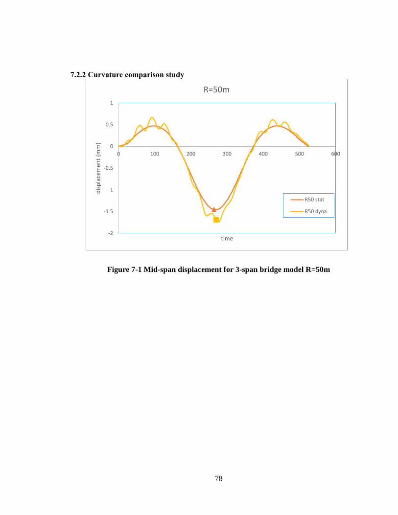
78
7.2.2 Curvature comparison study
Figure 7-1 Mid-span displacement for 3-span bridge model R=50m
-2
-1.5
-1
-0.5
0
0.5
1
0 100 200 300 400 500 600
dis
pla
cem
ent
(mm
)
time
R=50m
R50 stat
R50 dyna

79
Figure 7-2 Mid-span shear force for 3-span bridge model R=50m
Figure 7-3 Mid-span moment for 3-span bridge model R=50m
-200
-150
-100
-50
0
50
100
150
0 100 200 300 400 500 600
shea
r fo
rce
(KN
)
time
R=50m
R50 stat
R50 dyna
-600
-400
-200
0
200
400
600
0 100 200 300 400 500 600
mo
men
t (K
N m
)
time step
R=50m
R50 stat
R50 dyna

80
Figure 7-4 Mid-span displacement for 3-span bridge model R=75m
Figure 7-5 Mid-span shear force for 3-span bridge model R=75m
-1.6
-1.4
-1.2
-1
-0.8
-0.6
-0.4
-0.2
0
0.2
0.4
0.6
0 100 200 300 400 500 600
dis
pla
cem
ent
(mm
)
time
R=75m
R 75 Static
R 75 dyna
-250
-200
-150
-100
-50
0
50
100
150
200
0 100 200 300 400 500 600
shea
r fo
rce
(KN
)
time step
R=75m
R75 stat
R75 dyna

81
Figure 7-6 Mid-span moment for 3-span bridge model R=75m
Figure 7-7 Mid-span displacement for 3-span bridge model R=100m
-800
-600
-400
-200
0
200
400
600
0 100 200 300 400 500 600
mo
men
t (K
N m
)
time step
R=75m
R75 stat
R75 dyna
-1.4
-1.2
-1
-0.8
-0.6
-0.4
-0.2
0
0.2
0.4
0.6
0 100 200 300 400 500 600
dis
pla
cem
ent
(mm
)
time
R=100m
R100 static
R100 dyna

82
Figure 7-8 Mid-span shear force for 3-span bridge model R=100m
Figure 7-9 Mid-span shear force for 3-span bridge model R=100m
-200
-150
-100
-50
0
50
100
150
200
0 100 200 300 400 500 600
shea
r fo
rce
(KN
)
time
R=100m
R100 static
R100 dyna
-600
-500
-400
-300
-200
-100
0
100
200
300
400
500
0 100 200 300 400 500 600
mo
men
t (K
N m
)
time step
R=100m
R100 static
R100 dyna

83
Figure 7-10 Mid-span displacement for 3-span bridge model R=150m
Figure 7-11 Mid-span shear force for 3-span bridge model R=150m
-1.4
-1.2
-1
-0.8
-0.6
-0.4
-0.2
0
0.2
0.4
0 100 200 300 400 500 600
dis
pla
cem
ent
(mm
)
time
R=150m
R150 static
R150 dyna
-200
-150
-100
-50
0
50
100
150
0 100 200 300 400 500 600
shea
r fo
rce
(KN
)
time
R=150m
R150 static
R150 dyna

84
Figure 7-12 Mid-span shear force for 3-span bridge model R=150m
Figure 7-13 Mid-span displacement for 3-span bridge model R=190m
-600
-500
-400
-300
-200
-100
0
100
200
300
400
500
0 100 200 300 400 500 600
mo
men
t (K
N m
)
time step
R=150m
R150 static
R150 dyna
-1.2
-1
-0.8
-0.6
-0.4
-0.2
0
0.2
0.4
0 100 200 300 400 500 600
dis
pla
cem
ent
(mm
)
time
R=190m
R 190 Static
R 190 dyna

85
Figure 7-14 Mid-span shear force for 3-span bridge model R=190m
Figure 7-15 Mid-span shear force for 3-span bridge model R=190m
-200
-150
-100
-50
0
50
100
150
0 100 200 300 400 500 600
shea
r fo
rce
(KN
)
time
R=190m
R 190 Static
R 190 dyna
-600
-500
-400
-300
-200
-100
0
100
200
300
400
500
0 100 200 300 400 500 600
mo
men
t (K
N m
)
time step
R=190m
R 190 Static
R 190 dyna

86
Figure 7-16 Mid-span displacement for 3-span bridge model R=300m
Figure 7-17 Mid-span shear force for 3-span bridge model R=300m
-1.2
-1
-0.8
-0.6
-0.4
-0.2
0
0.2
0.4
0 100 200 300 400 500 600
dis
pla
cem
ent
(mm
)
time
R=300m
R300 static
R300 dyna
-200
-150
-100
-50
0
50
100
150
0 100 200 300 400 500 600
shea
r fo
rce
(KN
)
time
R=300m
R300 static
R300 dyna

87
Figure 7-18 Mid-span shear force for 3-span bridge model R=300m
-600
-400
-200
0
200
400
600
0 100 200 300 400 500 600
mo
men
t (K
N m
)
time step
R=300m
R300 static
R300 dyna

88
7.2.3 Span lengths comparison study
Figure 7-19 Mid-span displacement for 3-span bridge model L=175m
Figure 7-20 Mid-span shear force for 3-span bridge model L=175m
-1.20E+00
-1.00E+00
-8.00E-01
-6.00E-01
-4.00E-01
-2.00E-01
0.00E+00
2.00E-01
4.00E-01
0 100 200 300 400 500 600
dis
pla
cem
ent
(mm
)
time
L=175m
Normal spanstatic
Normal spandynamic
-200
-150
-100
-50
0
50
100
150
0 100 200 300 400 500 600
shea
r fo
rce
(KN
)
time
L=175m
Normal SpanStatic
Normal SpanDynamic

89
Figure 7-21 Mid-span shear force for 3-span bridge model L=175m
Figure 7-22 Mid-span displacement for 3-span bridge model L=235m
-600
-500
-400
-300
-200
-100
0
100
200
300
400
500
0 100 200 300 400 500 600
mo
men
t (K
N m
)
time step
L=175m
Normal SpanStatic
Normal SpanDynamic
-1.40E+00
-1.20E+00
-1.00E+00
-8.00E-01
-6.00E-01
-4.00E-01
-2.00E-01
0.00E+00
2.00E-01
4.00E-01
6.00E-01
0 100 200 300 400 500 600
dis
pla
cem
ent
(mm
)
time
L=235m
Long spanstatic
long spandynamic

90
Figure 7-23 Mid-span shear force for 3-span bridge model L=235m
Figure 7-24 Mid-span shear force for 3-span bridge model L=235m
-200
-150
-100
-50
0
50
100
150
0 100 200 300 400 500 600
shea
r fo
rce
(KN
)
time
L=235m
Long Span Static
Long Span Dynamic
-600
-500
-400
-300
-200
-100
0
100
200
300
400
500
0 100 200 300 400 500 600
mo
men
t (K
N m
)
time step
L=235m
Long SpanStatic
Long SpanDynamic

91
Figure 7-25 Mid-span displacement for 3-span bridge model L=120m
Figure 7-26 Mid-span shear force for 3-span bridge model L=120m
-0.6
-0.5
-0.4
-0.3
-0.2
-0.1
0
0.1
0.2
0.3
0 100 200 300 400 500 600
dis
pla
cem
ent
(mm
)
time
L=120m
short spanstatic
short spandynamic
-200
-150
-100
-50
0
50
100
150
0 100 200 300 400 500 600
shea
r fo
rce
(KN
)
time
L=120m
Short SpanStatic

92
Figure 7-27 Mid-span shear force for 3-span bridge model L=120m
7.2.4 Vehicle travelling speeds comparison study
Figure 7-28 Mid-span displacement for 3-span bridge model v=20m/s
-600
-400
-200
0
200
400
600
0 100 200 300 400 500 600
mo
men
t (K
N m
)
time step
L=120m
Short SpanStatic
Short SpanDynamic
-1.2
-1
-0.8
-0.6
-0.4
-0.2
0
0.2
0.4
-50 50 150 250 350 450 550
dis
pla
cem
ent
(mm
)
time
vehicle travelling at 20m/s
v=20
staticresponse

93
Figure 7-29 Mid-span displacement for 3-span bridge model v=30m/s
Figure 7-30 Mid-span displacement for 3-span bridge model v=40m/s
-1.4
-1.2
-1
-0.8
-0.6
-0.4
-0.2
0
0.2
0.4
0.6
-50 50 150 250 350 450 550
dis
pla
cem
ent
(mm
)
time
vehicle travelling at 30m/s
v=30
staticresponse
-1.4
-1.2
-1
-0.8
-0.6
-0.4
-0.2
0
0.2
0.4
0.6
-50 50 150 250 350 450 550
dis
pla
cem
ent
(mm
)
time
vehicle travelling at 40m/s
v=40
staticresponse

94
Figure 7-31 Mid-span displacement for 3-span bridge model v=50m/s
Figure 7-32 Mid-span displacement for 3-span bridge model v=60m/s
-1.4
-1.2
-1
-0.8
-0.6
-0.4
-0.2
0
0.2
0.4
0.6
0 100 200 300 400 500 600
dis
pla
cem
ent
(mm
)
time
vehicle traveling at 50m/s
v=50
static response
-2
-1.5
-1
-0.5
0
0.5
1
0 100 200 300 400 500 600
dis
pla
cem
ent
(mm
)
time
vehicle traveling at 60m/s
v=60
static response

95
Figure 7-33 Mid-span displacement for 3-span bridge model v=70m/s
-2
-1.5
-1
-0.5
0
0.5
1
0 100 200 300 400 500 600
dis
pla
cem
ent
(mm
)
time
vehicle traveling at 70m/s
v=70
static response

96
7.2.5 Deck roughness comparison study
Figure 7-34 Mid-span displacement for 3-span bridge model v=30m/s L=235m
perfect surface condition
Figure 7-35 Mid-span displacement for 3-span bridge model v=30m/s L=235m
good surface condition
-4
-3.5
-3
-2.5
-2
-1.5
-1
-0.5
0
0.5
1
1.5
0 100 200 300 400 500 600
dis
pla
cem
ent
(mm
)
time
Perfect condition
R 190Static
R 190 dyna
-4
-3
-2
-1
0
1
2
0 100 200 300 400 500 600
dis
pla
cem
ent
(mm
)
time
Good condition
R190 static
R190 dyna

97
Figure 7-36 Mid-span displacement for 3-span bridge model v=30m/s L=235m
normal surface condition
Figure 7-37 Mid-span displacement for 3-span bridge model v=30m/s L=235m
bad surface condition
-4
-3
-2
-1
0
1
2
0 100 200 300 400 500 600
dis
pla
cem
ent
(mm
)
time
Normal condition
R190 static
R190 dyna
-5
-4
-3
-2
-1
0
1
2
0 100 200 300 400 500 600
dis
pla
cem
ent
(mm
)
time
Bad condition
R 190Static
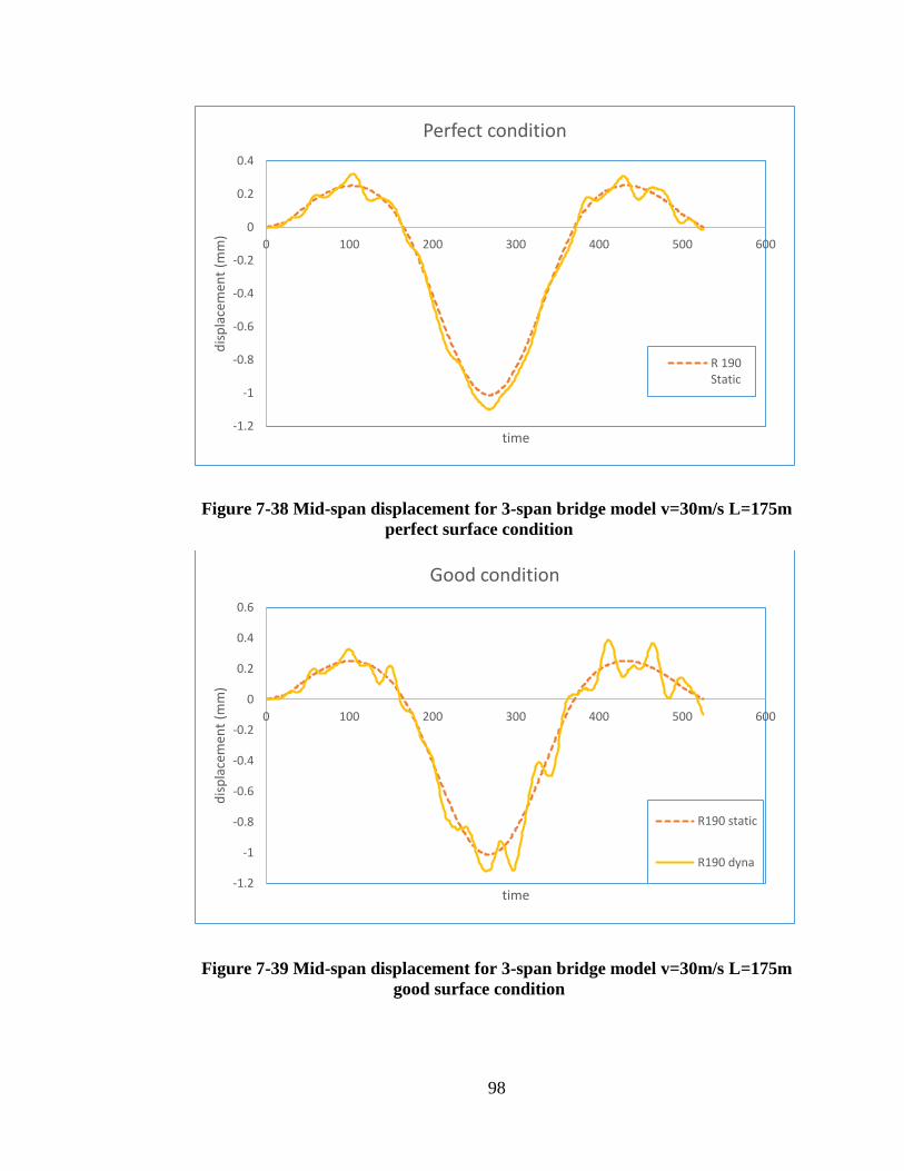
98
Figure 7-38 Mid-span displacement for 3-span bridge model v=30m/s L=175m
perfect surface condition
Figure 7-39 Mid-span displacement for 3-span bridge model v=30m/s L=175m
good surface condition
-1.2
-1
-0.8
-0.6
-0.4
-0.2
0
0.2
0.4
0 100 200 300 400 500 600
dis
pla
cem
ent
(mm
)
time
Perfect condition
R 190Static
-1.2
-1
-0.8
-0.6
-0.4
-0.2
0
0.2
0.4
0.6
0 100 200 300 400 500 600
dis
pla
cem
ent
(mm
)
time
Good condition
R190 static
R190 dyna

99
Figure 7-40 Mid-span displacement for 3-span bridge model v=30m/s L=175m
normal surface condition
Figure 7-41 Mid-span displacement for 3-span bridge model v=30m/s L=175m
bad surface condition
-2
-1.5
-1
-0.5
0
0.5
1
0 100 200 300 400 500 600
dis
pla
cem
ent
(mm
)
time
Normal condition
R190 static
R190 dyna
-2.5
-2
-1.5
-1
-0.5
0
0.5
1
1.5
0 100 200 300 400 500 600
dis
pla
cem
ent
(mm
)
time
Bad condition
R 190 Static
R 190 dyna

100
Figure 7-42 Mid-span displacement for 3-span bridge model v=30m/s L=120m
perfect surface condition
Figure 7-43 Mid-span displacement for 3-span bridge model v=30m/s L=120m
good surface condition
-0.6
-0.5
-0.4
-0.3
-0.2
-0.1
0
0.1
0.2
0 100 200 300 400 500 600
dis
pla
cem
ent
(mm
)
time
Perfect condition
R 190Static
-0.7
-0.6
-0.5
-0.4
-0.3
-0.2
-0.1
0
0.1
0.2
0.3
0 100 200 300 400 500 600
dis
pla
cem
ent
(mm
)
time
Good condition
R190 static
R190 dyna

101
Figure 7-44 Mid-span displacement for 3-span bridge model v=30m/s L=120m
normal surface condition
Figure 7-45 Mid-span displacement for 3-span bridge model v=30m/s L=120m
normal surface condition
-1
-0.8
-0.6
-0.4
-0.2
0
0.2
0.4
0.6
0 100 200 300 400 500 600
dis
pla
cem
ent
(mm
)
time
Normal condition
R190 static
R190 dyna
-1
-0.8
-0.6
-0.4
-0.2
0
0.2
0.4
0.6
0 100 200 300 400 500 600
dis
pla
cem
ent
(mm
)
time
Bad condition
R 190Static

102
7.2.6 Eccentricity study
Figure 7-46 Mid-span displacement for 3-span bridge model with vehicle
traveling through inner lane
Figure 7-47 Mid-span displacement for 3-span bridge model with vehicle
traveling through center lane
-1.2
-1
-0.8
-0.6
-0.4
-0.2
0
0.2
0.4
0 100 200 300 400 500 600
dis
pla
cem
ent
(mm
)
time
Eccentricity -3.0m
R 190 Static
R 190 dyna
-1.4
-1.2
-1
-0.8
-0.6
-0.4
-0.2
0
0.2
0.4
0 100 200 300 400 500 600
dis
pla
cem
ent
(mm
)
time
Eccentricity +0.0m
R190 static
R190 dyna

103
Figure 7-48 Mid-span displacement for 3-span bridge model with vehicle
traveling through outer lane
-1.4
-1.2
-1
-0.8
-0.6
-0.4
-0.2
0
0.2
0.4
0 100 200 300 400 500 600d
isp
lace
men
t (m
m)
time
Eccentricity +3.0m
R 190 Static
R 190 dyna

104
7.2.7 For 2-span bridge configurations
Figure 7-49 Mid-span displacement for 2-span bridge model v=20m/s
Figure 7-50 Mid-span displacement for 2-span bridge model v=30m/s
-2.500
-2.000
-1.500
-1.000
-0.500
0.000
0.500
1.000
1.500
0 100 200 300 400 500 600
dis
pla
cem
ent
(mm
)
time
vehicle speed 20m/s
R 190 Static
R 190 dyna
-2.500
-2.000
-1.500
-1.000
-0.500
0.000
0.500
1.000
1.500
0 100 200 300 400 500 600
dis
pla
cem
ent
(mm
)
time
vehicle speed 30m/s
R190 static
R190 dyna

105
Figure 7-51 Mid-span displacement for 2-span bridge model v=40m/s
Figure 7-52 Mid-span displacement for 2-span bridge model v=50m/s
-3.000
-2.500
-2.000
-1.500
-1.000
-0.500
0.000
0.500
1.000
1.500
0 100 200 300 400 500 600
dis
pla
cem
ent
(mm
)
time
vehicle speed 40m/s
R190 static
R190 dyna
-2.500
-2.000
-1.500
-1.000
-0.500
0.000
0.500
1.000
1.500
2.000
0 100 200 300 400 500 600
dis
pla
cem
ent
(mm
)
time
vehicle speed 50m/s
R190 static
R190 dyna

106
Figure 7-53 Mid-span displacement for 2-span bridge model v=60m/s
-3.000
-2.500
-2.000
-1.500
-1.000
-0.500
0.000
0.500
1.000
1.500
2.000
2.500
0 100 200 300 400 500 600
dis
pla
cem
ent
(mm
)
time
vehicle speed 60m/s
R190 stat
R190 dyna

107
Figure 7-54 Mid-span displacement for 2-span bridge model v=70m/s
7.3 Discussion of Results
The results of the interaction analysis are evaluated by comparing the mid-span
dynamic reactions with the static reactions. In the case of curvature radii study, it can be
noted that as the radius increase, the bridge displacement, shear and moment reactions
tend to become more stable. By evaluating the displacement reactions, it can be further
noticed how the dynamic interaction is influenced by the curvature (as demonstrated in
figure 7.55). As the radius increase, both static and dynamic displacement responses are
lowered, while the differences of dynamic and static reactions also decline and start to
stabilize after reaching R=150m (Figure 7.56). The difference (%) in the figure can be
defined as:
-2.500
-2.000
-1.500
-1.000
-0.500
0.000
0.500
1.000
1.500
2.000
2.500
0 100 200 300 400 500 600
dis
pla
cem
ent
(mm
)
time
vehicle speed 70m/s
R190 stat
R190 dyna

108
𝐷𝑖𝑓𝑓𝑒𝑟𝑒𝑛𝑐𝑒 =𝑑𝐷−𝑑𝑆
𝑑𝑆× 100% (7.1)
Where dD is the maximum absolute displacement for center span mid-point under
dynamic vehicle load, and dS is the corresponding displacement under the same vehicle
static load. Such displacement difference percentage can be also considered as the
dynamic amplified factor (impact factor) during vehicle bridge interaction. When radius
is larger than 190m, the displacement impact factor stays around 7% to 9%. From
curvature radii R=190m to R=50m, the maximum dynamic displacement reaction as well
as the displacement dynamic impact factor increase rapidly. For the bridge configuration
whose radius is 50m, the impact factor is 19.43%, 2.5 times of the impact factor (7.8%)
from the original bridge configuration.
Figure 7-55 Displacement reactions with different radii
R=50 R=75 R=100 R=150 R=190 R=300
static 1.46034 1.15837 1.06572 1.0417 1.03344 1.03522
dynamic 1.74413 1.34711 1.20554 1.12937 1.11405 1.12302
0
0.2
0.4
0.6
0.8
1
1.2
1.4
1.6
1.8
2
dis
pla
cem
enT
(mm
)

109
Figure 7-56 Differences of displacement increment
From figures 7.57 to 7.59, the bridge moment response, like the displacement
response, has a relatively less influence in cases where the curvature radii is higher.
When the radii drop below R=150m, both the positive and negative moment responses
start to react dramatically, especially when the radius reach R=50m.
19.43%
16.29%
13.12%
8.42% 7.80%8.48%
0.00%
5.00%
10.00%
15.00%
20.00%
25.00%
R=50 R=75 R=100 R=150 R=190 R=300
incr
emen
tp
erce
nta
ge

110
Figure 7-57 mid-span moment comparison under different radii configurations
Figure 7-58 negative moment impact factors for different radii configurations
-600
-400
-200
0
200
400
600
0 100 200 300 400 500 600
mo
men
t (K
N m
)
time step
r=190
R=300
R=100
24.36%
19.96%
9.77%
5.32%
1.36%
8.48%
0.00%
5.00%
10.00%
15.00%
20.00%
25.00%
30.00%
R=50 R=75 R=100 R=150 R=190 R=300
incr
emen
tp
erce
nta
ge

111
Figure 7-59 positive moment impact factors for different radii configurations
Bridge reactions from three different span length are gathered to study the influence
of span length in vehicle bridge interaction. Figures 7.60 to 7.61 show summarize the
maximum displacements and displacement impact factors of different configurations.
Generally, with the increasing of span length, the bridge flexibility also increased. Bridge
starts to increase the capability to absolve dynamic impact and reduce its effect on
structure, thereafter has lowered the impact factors. In these parametric study cases, it can
be observed that, though the maximum static displacements increase with the span length,
dynamic displacements do not have a higher increment rate, which lead to lower impact
factor.
60.93%
46.22%
23.70%20.43%
9.51%
15.15%
0.00%
10.00%
20.00%
30.00%
40.00%
50.00%
60.00%
70.00%
R=50 R=75 R=100 R=150 R=190 R=300
incr
emen
tp
erce
nta
ge
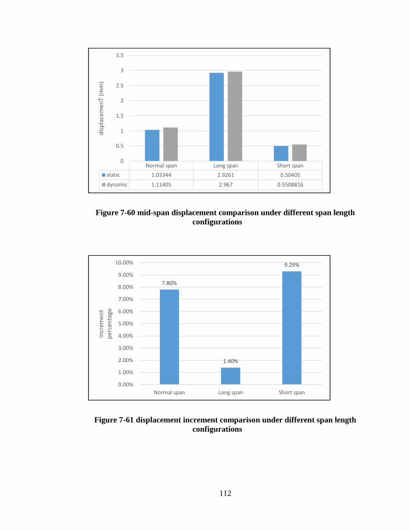
112
Figure 7-60 mid-span displacement comparison under different span length
configurations
Figure 7-61 displacement increment comparison under different span length
configurations
Normal span Long span Short span
static 1.03344 2.9261 0.50405
dynamic 1.11405 2.967 0.5508816
0
0.5
1
1.5
2
2.5
3
3.5
dis
pla
cem
enT
(mm
)
7.80%
1.40%
9.29%
0.00%
1.00%
2.00%
3.00%
4.00%
5.00%
6.00%
7.00%
8.00%
9.00%
10.00%
Normal span Long span Short span
incr
emen
tp
erce
nta
ge

113
Figure 7.62 summarizes the displacement impact factors of bridge of different deck
conditions and exciting vehicle traveling with various speed. Although the initial bridge
reaction is rather small (less than 10% under different surfaces), the impact factors start
to raise with an alarming speed after vehicle reaching certain travelling speed. When the
vehicle speed reach the maximum in this analysis, the impact factor is over 0.6 in all
cases, at this point the factor of vehicle travelling speed overshadows other factors such
as bridge surface conditions.
Figure 7-62 Amplified factors vs. surface condition vs. vehicle (Normal span
case)
1
1.1
1.2
1.3
1.4
1.5
1.6
1.7
1.8
0 10 20 30 40 50 60 70 80
Am
plif
ied
fac
tor
(I+1
)
vehicle speed
maximum amplified factor vs. surface and speed(normal span case)
perfect surface
Good surface
Normal surface
Bad surface

114
Following Table 7.1 and Figure 7.63 summarize the influence of bridge surface
condition to the vehicle bridge interaction analysis. It can be easily observed that with
“Perfect” and “Good” surface conditions, the impact factors are below 10% and 20%
respectivily. With the deteriating of the bridge surface, the dynamic impact load increases
dramatically. When the surface condition reaches “Bad”, the impact factor could be as
high as 99% even though the vehicle traveling speed is still low. At such case, a near-
resonance vibration is probably to happen which leads to a unusually high response. The
displacement reaction (Figure 7.12d) shows even after the vehicle pass through the
observation point, the bridge vibration does not quickly die out like other cases. This is
also an indication of near-resonance vibration occours.
Table 7-1 Impact factors (If) and Amplication factors (1+If) of different
surfaces and span configurations
table of impact factor
surface condition
Perfect Good Normal Bad
Long span bridge 1.014 1.066 1.090 1.200
1.40% 6.61% 9.05% 19.98%
Normal span bridge
1.078 1.108 1.525 1.994
7.80% 10.78% 52.53% 99.37%
Short span bridge 1.093 1.195 1.534 1.783
9.29% 19.54% 53.40% 78.28%

115
Figure 7-63 Impact factor of different surfaces and span configurations
Additional Figure 7.64 shows in the short span case (3 span total length =120m), the
dynamic factor increases with surface conditions and vehicle traveling speed. Although
both factors have positive impacts on the vehicle bridge interaction, the surface
conditions have influences. As the surface condition deteriorates, the influence of vehicle
speed in the dynamic interaction increases
1.40%6.61% 9.05%
19.98%7.80%
10.78%
52.53%
99.37%
9.29%19.54%
53.40%
78.28%
0.00%
20.00%
40.00%
60.00%
80.00%
100.00%
120.00%
Perfect Good Normal Bad
incr
emen
tp
erce
nta
ge

116
Figure 7-64 Amplified factors vs. surface condition vs. vehicle (Short span case)
A comparison is made in Figure 7.65 for eccentricity influence in vehicle bridge
interaction. It can be observed that though generally the outer lane loading leads to higher
impact factor. The difference in outer lane impact factor and inner lane impact factor is
hardly noticeable compared to other factors such as speed and surface conditions.
1
1.2
1.4
1.6
1.8
2
2.2
2.4
2.6
0 10 20 30 40 50 60 70 80
Am
plif
ied
fac
tor
(I+1
)
vehicle speed
maximum amplified factor vs. surface and speed (short span case)
perfect condition
good condition
normal condition
bad condition

117
Figure 7-65 Impact factor for different eccentricity
1.55% 1.40%1.72%
3.84%3.55%
4.58%
0.00%
1.00%
2.00%
3.00%
4.00%
5.00%
e=-3 e=0 e=+3
IMPACT FACTOR FOR DIFFERENT ECCENTRICITY
3 span normal length 2 span normal length

118
8. Calculation of Impact Factor
8.1 Calculation based on bridge natural frequency
From previous parametric study, the dynamic interaction usually leads to higher
dynamic load than static loading. Factors such as the surface conditions can have a
decisive and random influence on the dynamic interaction analysis. The location of
maximum dynamic reaction can occur at various points and different static reaction
locations. Therefore, in this study, the maximum displacement during the interaction
period is selected for the impact factor calculation. The empirical formula for impact
factor is categorized by the bridge surface conditions and bridge speed limits. The bridge
material and geometric property can be simplified as the bridge first flexural frequency in
the empirical formula. The frequencies of the parametric study are summarized in Table
8.1.

119
Table 8-1 First flexural frequencies of parametric bridge cases.
Radius
bridge configuration R 300 R 250 R 190 R 150 R 100 R50
3 Span
120m length 3.614 3.603 3.5828 3.512 3.456 3.13466
175m length 1.88 1.8644 1.8478 1.8037 1.741 1.39123
235m length 0.8268 0.8251 0.825 0.8226 0.82 1.0047
2 Span
100m length 2.4889 2.454 2.369 2.253 2.198 2.04915
150m length 1.8786 1.806 1.7038 1.621 1.5523 1.5047
190m length 1.16835 1.1564 1.256 1.0062 1.0011 0.92867
Figures 8.1 to 8.12 collect the impact factors for different case scenarios and show
the impact factor tendency line. To better cover the different demands for dynamic load
allowance, three different categories are set in this study.
A. Design criteria (perfect surface) for low speed limit bridge (V=20m/s, 45mph),
B. Design criteria (perfect surface) for high speed limit bridge (V=30m/s, 65mph)
C. Service criteria (good surface condition) for low speed limit bridge (V=20m/s,
45mph).

120
The formula is based on the bridge configurations from the previous parametric
study cases. The cases include two and three span bridges with total spans ranging from
120m to 235m, radii ranging from 50m to 300m. The impact factor in this formula
describe the center span maximum displacement, moment, torsion and shear dynamic
reactions.
The displacement impact factor (I) can be expressed by the bridge frequency (ν) as
follows:
a. For low speed limit bridge design
𝐼 = 0.05 + 0.113ν (0.5 ≤ ν ≤ 1.5)
0.22 (1.5 < ν ≤ 4) (8.1)
b. For high speed limit bridge design
𝐼 = 0.05 + 0.12ν (0.5 ≤ ν ≤ 1.5)
0.23 (1.5 < ν ≤ 4) (8.2)
c. For low speed limit bridge service
𝐼 = 0.05 + 0.133ν (0.5 ≤ ν ≤ 1.5)
0.25 (1.5 < ν ≤ 4) (8.3)
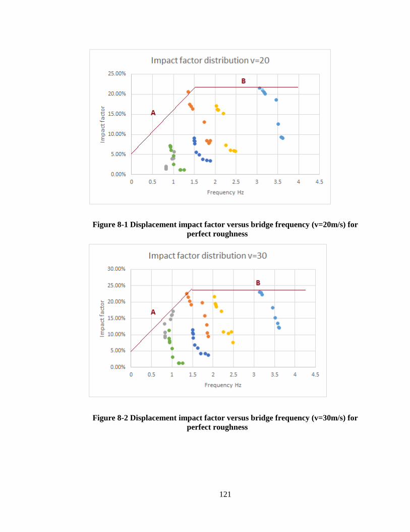
121
Figure 8-1 Displacement impact factor versus bridge frequency (v=20m/s) for
perfect roughness
Figure 8-2 Displacement impact factor versus bridge frequency (v=30m/s) for
perfect roughness

122
Figure 8-3 Displacement impact factor versus bridge frequency (v=20m/s) for
wearing deck
The moment impact factor (I) can be expressed by the bridge frequency (ν) as
follows:
a. For low speed limit bridge design
𝐼 = 0.025 + 0.11ν (0.5 ≤ ν ≤ 1.5)
0.19 (1.5 < ν ≤ 4) (8.4)
b. For high speed limit bridge design
𝐼 = 0.05 + 0.123ν (0.5 ≤ ν ≤ 1.5)
0.21 (1.5 < ν ≤ 4) (8.5)

123
c. For low speed limit bridge service
𝐼 = 0.05 + 0.117ν (0.5 ≤ ν ≤ 1.5)
0.225 (1.5 < ν ≤ 4) (8.6)
Figure 8-4 Moment impact factor versus frequency (v=20m/s) for perfect
roughness

124
Figure 8-5 Moment Impact factor versus bridge frequency (v=30m/s) for
perfect roughness
Figure 8-6 Impact factor versus bridge frequency (v=20m/s) for wearing deck
The torsional impact factor (I) can be expressed by the bridge frequency (ν) as
follows:
a. For low speed limit bridge design
𝐼 = 0.025 + 0.117ν (0.5 ≤ ν ≤ 1.5)
0.20 (1.5 < ν ≤ 4) (8.7)
b. For high speed limit bridge design
𝐼 = 0.025 + 0.147ν (0.5 ≤ ν ≤ 1.5)
0.245 (1.5 < ν ≤ 4) (8.8)

125
c. For low speed limit bridge service
𝐼 = 0.168ν (0.5 ≤ ν ≤ 1.25)
0.21 (1.25 < ν ≤ 4) (8.9)
Figure 8-7 Torsional impact factor versus frequency (v=20m/s) for perfect
roughness

126
Figure 8-8 Torsional impact factor versus frequency (v=30m/s) for perfect
roughness
Figure 8-9 Torsional impact factor versus bridge frequency (v=20m/s) for
wearing deck

127
The shear impact factor (I) can be expressed by the bridge frequency (ν) as follows:
d. For low speed limit bridge design
𝐼 = 0.155 (0.5 ≤ ν ≤ 4) (8.10)
e. For high speed limit bridge design
𝐼 = 0.2 (0.5 ≤ ν ≤ 4) (8.11)
f. For low speed limit bridge service
𝐼 = 0.22 (0.5 ≤ ν ≤ 4) (8.12)
Figure 8-10 Shear impact factor versus frequency (v=20m/s) for perfect
roughness

128
Figure 8-11 Shear impact factor versus frequency (v=30m/s) for perfect
roughness
Figure 8-12 Shear impact factor versus bridge frequency (v=20m/s) for wearing
deck

129
The empirical formulas generated above are a simplified method to calculate
dynamic impact factors based on the bridge parametric study cases. Therefore, this
formula should only apply to bridges with similar configurations and highway design
parameters. Other empirical formulas are required for other types of bridges.
By comparing the different impact factor equations, it can be observed that
displacement impact factor trend to be the highest among these dynamic factors. A
comparison of different determining methods of displacement impact factor is
summarized in Figure 8.13. The AASHTO LRFD Bridge Design specification 2017
consider most of the bridge components has a constant dynamic impact factor of 0.33 and
0.15 regardless of bridge configurations. While Canadian codes OHDBC 1982 and
CHBDC 2000 both show similar impact factor develop trend as the current research, the
impact factors increase as the bridge flexural frequency increase. All three impact factor
determining methods have their fix maximum points for the impact factor. However, as
the current study shows, the impact factor is heavily influenced by the bridge surface
condition. As the bridge deck starts wearing off during the service period, the impact
factor will rise rapidly and most likely grow beyond the limits set by AASHTO and
OHDBC codes.

130
Figure 8-13 Comparison of different methods of determining impact factors
8.2 Calculation based on bridge central angle
There are multiple factors that affect the dynamic interaction in curved bridge.
Another well accepted way to represent curved bridge property is to introduce curvature
central angle (ϕ=L/R) in the formula. Similar to previous formula, this empirical formula
for impact factor is categorized by bridge surface conditions and bridge speed limits. The
bridge material and geometric property can be simplified as the bridge central angle in

131
the empirical formula. The central angles of the parametric study are summarized in the
Table 8.2.
Table 8-2 Central angles of parametric bridge cases.
bridge configuration Radius
R 300 R 250 R 190 R 150 R 100 R60 R55 R50 R40
3 Span 120m length 0.400 0.480 0.632 0.800 1.200 2.000 2.182 2.400 3.000
175m length 0.583 0.700 0.921 1.167 1.750 2.917 3.182 3.500 4.375
235m length 0.783 0.940 1.237 1.567 2.350 3.917 4.273 4.700 5.875
2 Span 100m length 0.333 0.400 0.526 0.667 1.000 1.667 1.818 2.000 2.500
150m length 0.500 0.600 0.789 1.000 1.500 2.500 2.727 3.000 3.750
190m length 0.633 0.760 1.000 1.267 1.900 3.167 3.455 3.800 4.750
Figures 8.14 to 8.25 collect the impact factors for different case scenarios and show
the impact factor tendency lines. Same three different categories are set in study.
a. Design criteria (perfect surface) for low speed limit bridge (V=20m/s,
45mph),
b. Design criteria (perfect surface) for high speed limit bridge (V=30m/s,
65mph)
c. Service criteria (good surface condition) for low speed limit bridge (V=20m/s,
45mph).
The formula is based on bridge configurations from the previous parametric study
cases. The cases include two and three span bridges with total spans ranging from 120m
to 235m, radii ranging from 40m to 300m. The impact factors in this formula describe the
center span maximum displacement dynamic reaction.

132
The displacement impact factor (I) can be expressed by the central angle (ϕ) as
follows:
a. For low speed limit bridge design
𝐼 = 0.05 + 0.136ϕ (0 ≤ ϕ ≤ 1.25)
0.22 (1.25 < ϕ ≤ 4.5) (8.13)
b. For high speed limit bridge design
𝐼 = 0.10 + 0.0867ϕ (0 ≤ ϕ ≤ 1.5)
0.23 (1.5 < ϕ ≤ 4.5) (8.14)
c. For low speed limit bridge service
𝐼 = 0.15 + 0.10ϕ (0 ≤ ϕ ≤ 1.0)
0.25 (1.0 < ϕ ≤ 4.5) (8.15)

133
Figure 8-14 Displacement Impact factor versus bridge central angle (v=20m/s)
for perfect roughness
Figure 8-15 Displacement Impact factor versus bridge central angle (v=30m/s)
for perfect roughness

134
Figure 8-16 Displacement Impact factor versus bridge frequency (v=20m/s) for
wearing deck
The moment impact factor (I) can be expressed by the central angle (ϕ) as follows:
a. For low speed limit bridge design
𝐼 = 0.07 + 0.096ϕ (0 ≤ ϕ ≤ 1.25)
0.19 (1.25 < ϕ ≤ 4.5) (8.16)
b. For high speed limit bridge design
𝐼 = 0.09 + 0.08ϕ (0 ≤ ϕ ≤ 1.5)
0.21 (1.5 < ϕ ≤ 4.5) (8.17)
c. For low speed limit bridge service
𝐼 = 0.15 + 0.075ϕ (0 ≤ ϕ ≤ 1.0)
0.225 (1.0 < ϕ ≤ 4.5) (8.18)

135
Figure 8-17 Moment impact factor versus bridge central angle (v=20m/s) for
perfect roughness
Figure 8-18 Moment impact factor versus bridge central angle (v=30m/s) for
perfect roughness

136
Figure 8-19 Moment impact factor versus bridge central angle (v=20m/s) for
wearing deck
The torsional impact factor (I) can be expressed by the central angle (ϕ) as follows:
a. For low speed limit bridge design
𝐼 = 0.05 + 0.12ϕ (0 ≤ ϕ ≤ 1.25)
0.20 (1.25 < ϕ ≤ 4.5) (8.19)
b. For high speed limit bridge design
𝐼 = 0.09 + 0.1033ϕ (0 ≤ ϕ ≤ 1.5)
0.245 (1.5 < ϕ ≤ 4.5) (8.20)
c. For low speed limit bridge service
𝐼 = 0.13 + 0.08ϕ (0 ≤ ϕ ≤ 1.0)
0.21 (1.0 < ϕ ≤ 4.5) (8.21)

137
Figure 8-20 Torsional impact factor versus bridge central angle (v=20m/s) for
perfect roughness
Figure 8-21 Torsional impact factor versus bridge central angle (v=30m/s) for
perfect roughness

138
Figure 8-22 Torsional impact factor versus bridge central angle (v=20m/s) for
wearing deck
The shear impact factor (I) can be expressed by the central angle (ϕ) as follows:
a. For low speed limit bridge design
𝐼 = 0.155 (ϕ ≤ 4.5) (8.22)
b. For high speed limit bridge design
𝐼 = 0.20 (ϕ ≤ 4.5) (8.23)
c. For low speed limit bridge service
𝐼 = 0.22 (ϕ ≤ 4.5) (8.24)

139
Figure 8-23 Shear impact factor versus bridge central angle (v=20m/s) for
perfect roughness
Figure 8-24 Shear impact factor versus bridge central angle (v=30m/s) for
perfect roughness

140
Figure 8-25 Torsional impact factor versus bridge central angle (v=20m/s) for
wearing deck
The empirical formulas generated above are a simplified supplementary method in
addition to the previous frequency depended method. In the cases of curved bridge
problem, the central angle of the bridge can better account for the effect of bridge
curvature property. From the parametric studies, it can be observed that for
displacement, moment and torsional impact factors, these impact factors achieve their
highest points when the bridge central angle reaches 1.0 (Slow traffic, wearing surface),
1.25 (Slow traffic, good surface) and 1.5 (Fast traffic, good surface). Combining the
experience from parametric study, this indicates that when the ϕ is small, as the curvature
radius decreases, the dynamic reaction increases dramatically.

141
9. Summary, Conclusions and Future Work
9.1 Summary and Conclusion
The objectives of this research are to study the vehicle-bridge interaction of curved
bridges. Including the difference of static interaction and straight bridge dynamic
interaction, the contribution of various factors in dynamic interaction are summarized.
Besides, a set of simplified empirical equations for calculating curved bridge dynamic
impact factor are finally developed.
Principles of vehicle-bridge interaction are presented along with the theoretical
background of the topic. A review of available literature indicated that thought on the
behavior of dynamic interaction is well recognized, however, there is no unified method
to determine the impact factor among the current researches and design specifications.
Besides, only few researches expanded the interaction topic to horizontally curved
bridges.
Two existing curved bridges, one in concrete and another in steel, are presented to
briefly demonstrate the behavior difference in vehicle-bridge interaction in horizontally
curved bridge scenario. To observe how the different parameters affect the vehicle-bridge
interaction, a detailed parametric study is conducted based on the existing steel curved
bridge. The mid-span reactions are focused and utilized to generate the dynamic load

142
impact factor. Observations and conclusions obtained from the studies can be
summarized as follows:
• Based on commercial software ANSYS Mechanical APDL command
interface, the interaction system is modeled as a three-beam gird bridge
model and a 24 degree-of-freedom 3-dimension truck model. These two
subsystems are connected using simplified discrete iterative algorithm. The
effects, such as bridge deck conditions and traffic speed, are introduced in
the iterative algorithm and discussed extensively to study their influence in
vehicle-bridge interaction problem.
• The curvature of the bridge horizontal layout has a noticeable effect on the
vehicle-bridge interaction due to torsional effects and centrifugal forces. The
parametric study shows a sharp turning bridge can be observed a
considerable increment of impact factor. As the radius increases (e.g. less
curved) the impact factor generally reduces, once the radius reaches certain
threshold the impact factors convergence into the value of straight bridge
impact factor.
• Bridge deck conditions and vehicle traveling speed are two major
contributors in the dynamic interaction. Parametric study shows at the bad
surface condition, the bridge could have a strong impact factor even the
vehicle traveling at a relative low speed. As the vehicle reaches certain
speed, the exciting frequency may resonance with the bridge, resulting a

143
much higher response behavior than the tendency shows. The occurrence of
such resonance speed varies with the vehicle and bridge properties.
• Other factors’ influences are also studied. The span length has a moderate
impact on the dynamic interaction. When the radius of bridge is given, a
longer span bridge leads to lower stiffness and more buffering space for
dynamic load, the impact factor is generally in an inverse ratio to the bridge
span length. Such observation agrees with the previous empirical function
given by Koichi (1985). The traffic lane location has limited influence on the
impact factor. For the case where traffic applies to the outer portion of the
curve, both stress and dynamic impact factor are higher than that of inner
portion of curve. However, such difference is marginal.
• The dynamic behaviors of torsion, shear and moment are also noticeable
under different model parameters. However, the displacement impact factor
of mid-span response is usually the most sensitive factor to the different
parameters. Such factor is considered to be the primary indicator of dynamic
interaction.
• To simplify the process of determining dynamic impact factor, the bridge
first flexural frequency is chosen to represent the bridge material and
geometric properties. Similar process is also adopted by Canadian code
OHDBC.
• A second method based on the bridge central angle is developed in order to
account for bridge curvature in determining dynamic impact factor. This

144
method is a supplementary method in addition to the frequency formula.
Such method does not require engineers to acquire the bridge natural
frequency when determining dynamic impact factor. Therefore, central angle
method is more favored in US by the bridge community.
• By observing massive data of different bridge configurations, vehicle
traveling pattern, the upper bound envelop curve of impact factor is
summarized. Based on such curve, a set of simple empirical equations is
made for the calculation of curved bridge impact factor. By comparing to the
current design specifications, the empirical equations show certain degree of
agreement in the lower bridge flexural frequency range. However, none of
the current codes sufficiently consider the extra dynamic load introduced by
a dilapidated surface condition. During the parametric study, it can be
frequently observed that the displacement impact factor climbs beyond the
0.75, which is the highest allowance provided in current design codes. Also,
the highway speed limit is ignored in current codes, for the highway where
speed limit is lower than 20m/s (45mph), the current codes will yield a much
conservative result.
9.1.1 Innovation in this study
The innovation and improvement provided in this study include:
• Improved the three-beam gird model based on shear-flexibility grillage
analyzing method. The warping effect and torsional inertia are considered
in the current model.

145
• Based on commercial software ANSYS Mechanical APDL command
interface, the effects such as bridge deck conditions and traffic speeds are
introduced in the vehicle-bridge-interaction system. A more detailed 24
degree-of-freedom, 3-dimension truck model is also integrated in the
study.
• Based on the massive data from different bridge configurations and
vehicle traveling pattern, the upper bound envelop curve of impact factor
is summarized. A practical and simplified empirical equation for dynamic
impact factor is summarized. Comments and suggestion are given by
comparing the current specifications of dynamic allowance.
9.2 Suggestions for future Work
More future research is required to further investigate the dynamic interaction of
curved bridge. These suggestions are listed below:
• One of the extensions for further work would be adding more vehicles
simultaneously on the same lane and/or on multiple lanes at the same time.
The extensive dynamic loading could expose a deeper insight into the
dynamic interaction under heavy traffic loads.
• The different parameters may be assigned to further investigate the influence
of empirical function of this study; for instance, the stiffness and damping of
the vehicles, bridge bearing types.

146
• In the current study, the impact factor empirical function is based on the box
steel girder bridge. Different bridge type should be introduced in further
studies in order to expand the compatibility of this calculation method.
• Current impact factor function is expressed in terms of bridge first flexural
frequency, similar to OHDBC specification. Some other researches conclude
that the flexural frequency function has its limitation in terms of accuracy. In
order to achieve a more comprehensive method, a better expression is
required.

147
10. Appendix -A
Source code for vehicle bridge interaction
ANSYS Mechanical APDL
Program mainframe:
3-span bridge interaction model
!!!!!!!!!mainframe
fini
/clear,start
/config,NRES,300000
/prep7
*create,para_def,mac
*dim,m_che,,4
*dim,k_che,,4
*dim,c_che,,4
k_che(1)=12147760,1838752,4186428,1045356 !vehicle stiffness infomation
c_che(1)=3e4,1.2e4,1.4e5,1.7e5

148
m_che(1)=945,480,20433,8592 !unit:kg vehicle weight
L=120 !The total span of bridge/m
dx=0.24 !element length corresponding to the sampling point
!delta_t=dx/v
E_num=L/dx !Enum of the bridge
pi=3.14159
!rmid=280
phi=L/rmid*180/pi
dphi=phi/E_num
*dim,dz_che1,,E_num+100 ! vehicle wheel contract point (speed)
*dim,dz_che2,,E_num+100
*dim,z_che1,,E_num+25 !vehicle wheel contract point (location)
*dim,z_che2,,E_num+25
*dim,jiasudu,,E_num+100
*dim,sudu_front,,E_num+100,100
*dim,sudu_back,,E_num+100,100
*dim,weiyi_front,,E_num+1,100

149
*dim,weiyi_back,,E_num+1,100
!*dim,yb_mid,,E_num+25
!*dim,Mb_mid,,E_num+25
!*dim,ys,,E_num+25
!*dim,Ms,,E_num+25
!*dim,disp_mid,,E_num+25,12
!*dim,moment_mid,,E_num+25,12
*dim,rx,,E_num+100 !surface condition information
*dim,drx,,E_num+100
*dim,disp_side,,550 !edge/center span displacement
*dim,disp_mid,,550
*dim,disp_side_L,,550
*dim,disp_mid_L,,550
*dim,disp_side_R,,550
*dim,disp_mid_R,,550
*dim,mx_side,,550 !edge span, moment torsion shear
*dim,my_side,,550

150
*dim,fz_side,,550
*dim,mx_zhi,,550
*dim,my_zhi,,550
*dim,fz_zhi,,550
*dim,mx_mid,,550 !center span, moment torsion etc.
*dim,my_mid,,550
*dim,fz_mid,,550
*dim,mz_dun,,550
*dim,fx_dun,,550
!store the maximum value for each required section
*dim,disp_side_max,,15,15
*dim,disp_mid_max,,15,15
*dim,disp_side_L_max,,15,15
*dim,disp_mid_L_max,,15,15
*dim,disp_side_R_max,,15,15
*dim,disp_mid_R_max,,15,15

151
*dim,mx_side_max,,15,15
*dim,my_side_max,,15,15
*dim,fz_side_max,,15,15
*dim,mx_zhi_max,,15,15
*dim,my_zhi_max,,15,15
*dim,fz_zhi_max,,15,15
*dim,mx_mid_max,,15,15
*dim,my_mid_max,,15,15
*dim,fz_mid_max,,15,15
*dim,mz_dun_max,,15,15
*dim,fx_dun_max,,15,15
!store the min value for each required section
*dim,disp_side_min,,15,15
*dim,disp_mid_min,,15,15
*dim,disp_side_L_min,,15,15
*dim,disp_mid_L_min,,15,15
*dim,disp_side_R_min,,15,15

152
*dim,disp_mid_R_min,,15,15
*dim,mx_side_min,,15,15
*dim,my_side_min,,15,15
*dim,fz_side_min,,15,15
*dim,mx_zhi_min,,15,15
*dim,my_zhi_min,,15,15
*dim,fz_zhi_min,,15,15
*dim,mx_mid_min,,15,15
*dim,my_mid_min,,15,15
*dim,fz_mid_min,,15,15
*dim,mz_dun_min,,15,15
*dim,fx_dun_min,,15,15
!matrix for storing
*dim,uz_side,,550,15 !edge displacement
*dim,uz_side_L,,550,15
*dim,uz_side_R,,550,15

153
*dim,uz_mid,,550,15 !center displacement
*dim,uz_mid_L,,550,15
*dim,uz_mid_R,,550,15
*dim,fmx_side,,550,15 !edge moment torsion shear
*dim,fmy_side,,550,15
*dim,ffz_side,,550,15
*dim,fmx_zhi,,550,15 !support moment torsion shear
*dim,fmy_zhi,,550,15
*dim,ffz_zhi,,550,15
*dim,fmx_mid,,550,15 !center moment torsion shear
*dim,fmy_mid,,550,15
*dim,ffz_mid,,550,15
*dim,fmz_dun,,550,15
*dim,ffx_dun,,550,15
!dynamic amplified factors
*dim,DAF_min,,15,20
*dim,DAF_max,,15,20

154
*end
*create,vehicle_bridge,mac
/PREP7
/COM,create the vehicle model
ET,1,COMBIN14,,,2
ET,2,MASS21,,,4 ! TWO-DIMENSIONAL MASS
ET,3,BEAM3
*do,i,1,4
R,i,k_che(i),c_che(i)
R,i+4,m_che(i)
*enddo
R,9,1,1,1
MP,EX,9,2E14
MP,DENS,9,0
N,10001:10005:2,,0:1:0.5

155
N,10002:10006:2,3.6,0:1:0.5
type,1
real,1
E,10001,10003
TYPE,1
REAL,2
E,10002,10004
type,1
real,3
E,10003,10005
TYPE,1
REAL,4
E,10004,10006
*do,i,1,4
type,2
real,i+4
E,10002+i

156
M,10002+i,UY ! MASTER DOF IN Y DIRECTION AT FREE END OF
SPRING
*enddo
TYPE,3
REAL,9
MAT,9
E,10005,10006
ALLS
D,10001,ALL,,,10002,1
D,10003,UX,,,10005,1
fini
/COM,create the bridge model
/prep7
et,15,beam4 !main girder
r,15,5.1478,74.326,3.4375 !steel
rmore,,3.4771,,,,3311
mp,ex,15,1.999e11 !steel

157
mp,dens,15,7500
et,16,beam4
r,16,2.4,0.288,0.800,2,1.2 !property of pier
RMORE,,0.721,,,,
mp,ex,16,3.45e10
mp,dens,16,2600
r,17,4.4647,65.8619,2.0522 !girder change section 1
rmore,,2.6034,,,,3311
r,18,4.4647,65.8619,2.0522 !girder change section 2
rmore,,2.6034,,,,3311
et,20,beam4 !rigid rod
mp,dens,20,0
mp,ex,20,3.45e14
mp,prxy,20,0.1667
R,20,1,1,1,1,1 !property of rigid rod
RMORE,,1,,,,

158
*afun,deg
*do,i,1,E_num+1 !create the load point
n,i,(rmid+ev)*cos((i-1)*dphi),(rmid+ev)*sin((i-1)*dphi),0.8
*enddo
*do,i,1001,E_num+1001 !create the beam element point
n,i,rmid*cos((i-1001)*dphi),rmid*sin((i-1001)*dphi)
*enddo
type,15
real,15
mat,15
*do,i,1001,E_num+1000 !main gird
e,i,i+1
*enddo

159
alls
nsel,s,loc,y,rmid*sin(0*dphi),rmid*sin(8*dphi)
nsel,a,loc,y,rmid*sin(145*dphi),rmid*sin(157*dphi)
nsel,a,loc,y,rmid*sin(345*dphi),rmid*sin(357*dphi)
nsel,a,loc,y,rmid*sin(494*dphi),rmid*sin(501*dphi)
nsel,r,loc,z,0
nsel,r,loc,x,50,300
esln,s,1,all
emodif,all,real,18
alls
n,3000,
type,16
real,16
mat,16
n,600,rmid*cos((151-1)*dphi),rmid*sin((151-1)*dphi),-0.5

160
n,616,rmid*cos((151-1)*dphi),rmid*sin((151-1)*dphi),-8.5
fill
n,650,rmid*cos((351-1)*dphi),rmid*sin((351-1)*dphi),-0.5
n,666,rmid*cos((351-1)*dphi),rmid*sin((351-1)*dphi),-8.5
fill
e,1151,600,3000
e,1351,650,3000
*do,i,1,16
e,599+i,600+i,3000
e,649+i,650+i,3000
*enddo
alls
n,700,rmid-2.5
n,701,rmid+2.5
n,702,(rmid-2.5)*cos(phi),(rmid-2.5)*sin(phi)
n,703,(rmid+2.5)*cos(phi),(rmid+2.5)*sin(phi)

161
n,786,(rmid-2.5)*cos(85*dphi),(rmid-2.5)*sin(85*dphi)
n,787,(rmid+2.5)*cos(85*dphi),(rmid+2.5)*sin(85*dphi)
n,788,(rmid-2.5)*cos(250*dphi),(rmid-2.5)*sin(250*dphi)
n,789,(rmid+2.5)*cos(250*dphi),(rmid+2.5)*sin(250*dphi) !displacement
observation points
type,20
real,20
mat,20
e,1001,700
e,1001,701
e,1501,702
e,1501,703
e,1:501,1001:1501
e,1086,786
e,1086,787
e,1251,788
e,1251,789
csys,1

162
nsel,s,node,,1,2000
nrotat,all
csys,0
alls
d,700,uz,,,703,1
d,616,all,,,666,50
fini
*end
!桥面不平度等级,共 5 个等级,生成 5 个宏文件
*create,addr0
*VREAD,rx(1),rx0,txt,,JIK,1,E_num+100 !reading surface
(F20.10)
*VREAD,drx(1),drx0,txt,,JIK,1,E_num+100 !
(F20.10)

163
*end
*create,addr1
*VREAD,rx(1),rx1,txt,,JIK,1,E_num+100
(F20.10)
*VREAD,drx(1),drx1,txt,,JIK,1,E_num+100 !
(F20.10)
*end
*create,addr2
*VREAD,rx(1),rx2,txt,,JIK,1,E_num+100 !
(F20.10)
*VREAD,drx(1),drx2,txt,,JIK,1,E_num+100 !
(F20.10)
*end
*create,addr3

164
*VREAD,rx(1),rx3,txt,,JIK,1,E_num+100 !
(F20.10)
*VREAD,drx(1),drx3,txt,,JIK,1,E_num+100 !
(F20.10)
*end
*create,addr4
*VREAD,rx(1),rx4,txt,,JIK,1,E_num+100 !
(F20.10)
*VREAD,drx(1),drx4,txt,,JIK,1,E_num+100 !
(F20.10)
*end
*create,addr5
*VREAD,rx(1),rx5,txt,,JIK,1,E_num+100 !
(F20.10)
*VREAD,drx(1),drx5,txt,,JIK,1,E_num+100 !

165
(F20.10)
*end
*create,vehicle_solu,mac
/COM,
/solu
ANTYPE,TRANS
TRNOPT,FULL,,,,,1
OUTPR,basic,LAST
OUTRES,ALL,last
timint,on
kbc,1
nsubst,1
*do,i,1,E_num+25
time,i*delta_t
alls
fdele,all,all

166
f,10003,fy,k_che(1)*rx(i)+c_che(1)*v*drx(i)
f,10004,fy,k_che(2)*rx(i+24)+c_che(2)*v*drx(i+24)
solve
*enddo
fini
!!!!
/post26
nsol,2,10003,u,y,uy_10003
nsol,3,10004,u,y,uy_10004
deriv,4,2
deriv,5,3
vget,z_che1,2,delta_t
vget,z_che2,3,delta_t
vget,dz_che1,4,delta_t
vget,dz_che2,5,delta_t
fini

167
*end
*create,vehicle_solu2,mac
/COM,
/solu
ANTYPE,TRANS
TRNOPT,FULL,,,,,1
OUTPR,basic,LAST
OUTRES,all,last
timint,on
kbc,1
nsubst,1
*do,i,1,E_num+25
*if,i,LE,24,then !
time,i*delta_t
fdele,all,all

168
f,10003,fy,k_che(1)*rx(i)+c_che(1)*v*drx(i)
f,10004,fy,k_che(2)*(rx(i+24)+weiyi_front(i,jj-
1))+c_che(2)*(v*drx(i+24)+sudu_front(i,jj-1))
solve
*elseif,i,GE,25,and,i,LE,E_num+1,then
time,i*delta_t
fdele,all,all
f,10003,fy,k_che(1)*(rx(i)+weiyi_back(i-24,jj-
1))+c_che(1)*(v*drx(i)+sudu_back(i-24,jj-1))
f,10004,fy,k_che(2)*(rx(i+24)+weiyi_front(i,jj-
1))+c_che(2)*(v*drx(i+24)+sudu_front(i,jj-1))
solve
*else
time,i*delta_t
fdele,all,all
f,10003,fy,k_che(1)*(rx(i)+weiyi_back(i-24,jj-
1))+c_che(1)*(v*drx(i)+sudu_back(i-24,jj-1))
f,10004,fy,k_che(2)*rx(i+24)+c_che(2)*v*drx(i+24)

169
solve
*endif
*enddo
fini
!!!!
/post26
nsol,2,10003,u,y,uy_10003
nsol,3,10004,u,y,uy_10004
deriv,4,2
deriv,5,3
vget,z_che1,2,delta_t
vget,z_che2,3,delta_t
vget,dz_che1,4,delta_t
vget,dz_che2,5,delta_t
fini
*end

170
*create,bridge_solu,mac
/solu
ANTYPE,TRANS
TRNOPT,FULL,,,,,1
OUTPR,V,LAST
OUTRES,V,last
timint,on
alphad,0.06
betad,0.00015
kbc,1
nsubst,2
*do,i,1,E_num+25
*if,i,LE,24,then
time,i*delta_t
fdele,all,all

171
f,i,fx,(m_che(2)+m_che(4))*v**2/(rmid+ev)
f,i,fz,-(m_che(2)+m_che(4))*10-k_che(2)*(rx(i+24)+weiyi_front(i,jj)-z_che2(i))-
c_che(2)*(v*drx(i+24)+sudu_front(i,jj)-dz_che2(i))
solve
*elseif,i,GE,25,and,i,LE,E_num+1,then
time,i*delta_t
fdele,all,all
f,i,fx,(m_che(2)+m_che(4))*v**2/(rmid+ev)
f,i,fz,-(m_che(2)+m_che(4))*10-k_che(2)*(rx(i+24)+weiyi_front(i,jj)-z_che2(i))-
c_che(2)*(v*drx(i+24)+sudu_front(i,jj)-dz_che2(i))
f,i-24,fx,(m_che(1)+m_che(3))*v**2/(rmid+ev)
f,i-24,fz,-(m_che(1)+m_che(3))*10-k_che(1)*(rx(i)+weiyi_back(i-24,jj)-
z_che1(i))-c_che(1)*(v*drx(i)+sudu_back(i-24,jj)-dz_che1(i))
solve
*else
time,i*delta_t
fdele,all,all
f,i-24,fx,(m_che(1)+m_che(3))*v**2/(rmid+ev)

172
f,i-24,fz,-(m_che(1)+m_che(3))*10-k_che(1)*(rx(i)+weiyi_back(i-24,jj)-
z_che1(i))-c_che(1)*(v*drx(i)+sudu_back(i-24,jj)-dz_che1(i))
solve
*endif
*enddo
fini
/post1
set,first
*do,i,1,E_num+25
set,near,1,,,i*delta_t
*if,i,LE,24,then
sudu_front(i,jj)=Vz(i)
weiyi_front(i,jj)=uz(i)
*elseif,i,GE,25,and,i,LE,E_num+1,then
sudu_front(i,jj)=Vz(i)
weiyi_front(i,jj)=uz(i)
sudu_back(i-24,jj)=Vz(i-24)

173
weiyi_back(i-24,jj)=uz(i-24)
*else
sudu_back(i-24,jj)=Vz(i-24)
weiyi_back(i-24,jj)=uz(i-24)
*endif
*enddo
fini
*end
*create,static_solu,mac
/solu
ANTYPE,TRANS
TRNOPT,FULL,,,,,1
OUTPR,V,LAST
OUTRES,V,last
timint,off

174
kbc,1
nsubst,1
*do,i,1,E_num+25
*if,i,LE,24,then
time,i
fdele,all,all
f,i,fz,-(m_che(2)+m_che(4))*10
solve
*elseif,i,GE,25,and,i,LE,E_num+1,then
time,i
fdele,all,all
f,i,fz,-(m_che(2)+m_che(4))*10
f,i-24,fz,-(m_che(1)+m_che(3))*10
solve
*else
time,i
fdele,all,all

175
f,i-24,fz,-(m_che(1)+m_che(3))*10
solve
*endif
*enddo
fini
*end
2-span bridge interaction model:
!!!!!!!!!
fini
/clear,start
/config,NRES,300000
/prep7

176
*create,para_def,mac
*dim,m_che,,4
*dim,k_che,,4
*dim,c_che,,4
k_che(1)=12147760,1838752,4186428,1045356
c_che(1)=3e4,1.2e4,1.4e5,1.7e5
m_che(1)=945,480,20433,8592
L=150 !The total span of bridge/m
dx=0.30 !element length corresponding to the sampling point
!delta_t=dx/v
E_num=L/dx !Enum of the bridge
pi=3.14159
!rmid=280
phi=L/rmid*180/pi
dphi=phi/E_num
*dim,dz_che1,,E_num+100
*dim,dz_che2,,E_num+100

177
*dim,z_che1,,E_num+25
*dim,z_che2,,E_num+25
*dim,jiasudu,,E_num+100
*dim,sudu_front,,E_num+100,100
*dim,sudu_back,,E_num+100,100
*dim,weiyi_front,,E_num+1,100
*dim,weiyi_back,,E_num+1,100
!*dim,yb_mid,,E_num+25
!*dim,Mb_mid,,E_num+25
!*dim,ys,,E_num+25
!*dim,Ms,,E_num+25
!*dim,disp_mid,,E_num+25,12
!*dim,moment_mid,,E_num+25,12
*dim,rx,,E_num+100
*dim,drx,,E_num+100
*dim,disp_side,,550
*dim,disp_mid,,550

178
*dim,disp_side_L,,550
*dim,disp_mid_L,,550
*dim,disp_side_R,,550
*dim,disp_mid_R,,550
*dim,mx_side,,550 !
*dim,my_side,,550
*dim,fz_side,,550
*dim,mx_zhi,,550
*dim,my_zhi,,550
*dim,fz_zhi,,550
*dim,mx_mid,,550
*dim,my_mid,,550
*dim,fz_mid,,550
*dim,mz_dun,,550
*dim,fx_dun,,550
*dim,disp_side_max,,15,15

179
*dim,disp_mid_max,,15,15
*dim,disp_side_L_max,,15,15
*dim,disp_mid_L_max,,15,15
*dim,disp_side_R_max,,15,15
*dim,disp_mid_R_max,,15,15
*dim,mx_side_max,,15,15
*dim,my_side_max,,15,15
*dim,fz_side_max,,15,15
*dim,mx_zhi_max,,15,15
*dim,my_zhi_max,,15,15
*dim,fz_zhi_max,,15,15
*dim,mx_mid_max,,15,15
*dim,my_mid_max,,15,15
*dim,fz_mid_max,,15,15
*dim,mz_dun_max,,15,15
*dim,fx_dun_max,,15,15

180
*dim,disp_side_min,,15,15
*dim,disp_mid_min,,15,15
*dim,disp_side_L_min,,15,15
*dim,disp_mid_L_min,,15,15
*dim,disp_side_R_min,,15,15
*dim,disp_mid_R_min,,15,15
*dim,mx_side_min,,15,15
*dim,my_side_min,,15,15
*dim,fz_side_min,,15,15
*dim,mx_zhi_min,,15,15
*dim,my_zhi_min,,15,15
*dim,fz_zhi_min,,15,15
*dim,mx_mid_min,,15,15
*dim,my_mid_min,,15,15
*dim,fz_mid_min,,15,15
*dim,mz_dun_min,,15,15
*dim,fx_dun_min,,15,15

181
*dim,uz_side,,550,15
*dim,uz_side_L,,550,15
*dim,uz_side_R,,550,15
*dim,uz_mid,,550,15 !
*dim,uz_mid_L,,550,15
*dim,uz_mid_R,,550,15
*dim,fmx_side,,550,15 !
*dim,fmy_side,,550,15
*dim,ffz_side,,550,15
*dim,fmx_zhi,,550,15 !
*dim,fmy_zhi,,550,15
*dim,ffz_zhi,,550,15
*dim,fmx_mid,,550,15 !
*dim,fmy_mid,,550,15
*dim,ffz_mid,,550,15

182
*dim,fmz_dun,,550,15 !
*dim,ffx_dun,,550,15
*dim,DAF_min,,15,20
*dim,DAF_max,,15,20
*end
*create,vehicle_bridge,mac
/PREP7
/COM,create the vehicle model
ET,1,COMBIN14,,,2 !
ET,2,MASS21,,,4 ! TWO-DIMENSIONAL MASS
ET,3,BEAM3
*do,i,1,4
R,i,k_che(i),c_che(i)
R,i+4,m_che(i)
*enddo
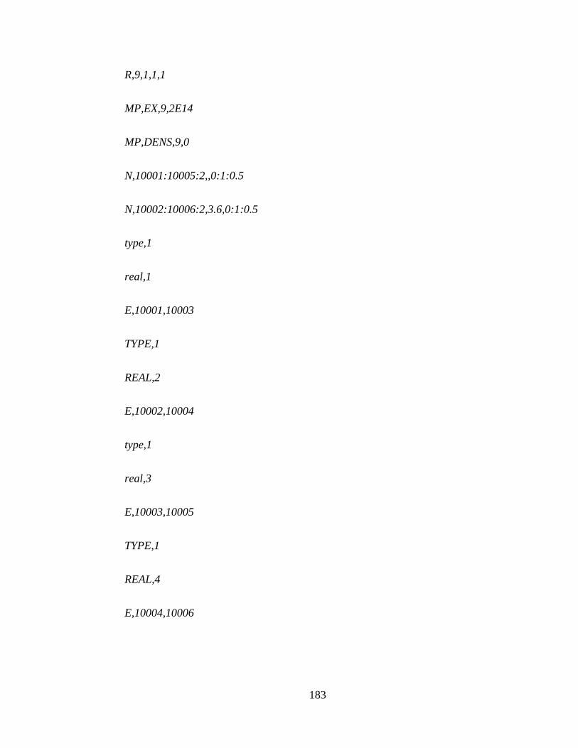
183
R,9,1,1,1
MP,EX,9,2E14
MP,DENS,9,0
N,10001:10005:2,,0:1:0.5
N,10002:10006:2,3.6,0:1:0.5
type,1
real,1
E,10001,10003
TYPE,1
REAL,2
E,10002,10004
type,1
real,3
E,10003,10005
TYPE,1
REAL,4
E,10004,10006

184
*do,i,1,4
type,2
real,i+4
E,10002+i
M,10002+i,UY ! MASTER DOF IN Y DIRECTION AT FREE END OF
SPRING
*enddo
TYPE,3
REAL,9
MAT,9
E,10005,10006
ALLS
D,10001,ALL,,,10002,1
D,10003,UX,,,10005,1
fini
/COM,create the bridge model
/prep7

185
et,15,beam4
r,15,6.4601,89.4805,5.224 !steel 材料
rmore,,4.0677,,,,3311
mp,ex,15,1.999e11 !steel
mp,dens,15,7500
et,16,beam4 !
r,16,2.4,0.288,0.800,2,1.2 !property of pier
RMORE,,0.721,,,,
mp,ex,16,3.45e10
mp,dens,16,2600
r,17,4.7408,67.8761,2.8008 !
rmore,,3.3924,,,,3311
r,18,4.7408,67.8761,2.8008 !
rmore,,3.3924,,,,3311
et,20,beam4
mp,dens,20,0

186
mp,ex,20,3.45e14
mp,prxy,20,0.1667
R,20,1,1,1,1,1 !property of rigid rod
RMORE,,1,,,,
*afun,deg
*do,i,1,E_num+1 !create the load point
n,i,(rmid+ev)*cos((i-1)*dphi),(rmid+ev)*sin((i-1)*dphi),0.8
*enddo
*do,i,1001,E_num+1001 !create the beam element point
n,i,rmid*cos((i-1001)*dphi),rmid*sin((i-1001)*dphi)
*enddo
type,15
real,15
mat,15

187
*do,i,1001,E_num+1000
e,i,i+1
*enddo
alls
nsel,s,loc,y,rmid*sin(0*dphi),rmid*sin(8*dphi)
nsel,a,loc,y,rmid*sin(145*dphi),rmid*sin(157*dphi)
nsel,a,loc,y,rmid*sin(345*dphi),rmid*sin(357*dphi)
nsel,a,loc,y,rmid*sin(494*dphi),rmid*sin(501*dphi)
nsel,r,loc,z,0
nsel,r,loc,x,50,300
esln,s,1,all
emodif,all,real,18
alls
n,3000,

188
type,16
real,16
mat,16
n,600,rmid*cos((251-1)*dphi),rmid*sin((251-1)*dphi),-0.5 !2span
configurations mid span pier
n,616,rmid*cos((251-1)*dphi),rmid*sin((251-1)*dphi),-8.5
fill
!n,650,rmid*cos((351-1)*dphi),rmid*sin((351-1)*dphi),-0.5
!n,666,rmid*cos((351-1)*dphi),rmid*sin((351-1)*dphi),-8.5
!fill
e,1251,600,3000
!e,1351,650,3000
*do,i,1,16
e,599+i,600+i,3000
!e,649+i,650+i,3000
*enddo
alls

189
n,700,rmid-2.5
n,701,rmid+2.5
n,702,(rmid-2.5)*cos(phi),(rmid-2.5)*sin(phi)
n,703,(rmid+2.5)*cos(phi),(rmid+2.5)*sin(phi)
n,786,(rmid-2.5)*cos(85*dphi),(rmid-2.5)*sin(85*dphi)
n,787,(rmid+2.5)*cos(85*dphi),(rmid+2.5)*sin(85*dphi) !edge span,
useless in 2span case
n,788,(rmid-2.5)*cos(125*dphi),(rmid-2.5)*sin(125*dphi)
n,789,(rmid+2.5)*cos(125*dphi),(rmid+2.5)*sin(125*dphi) !displacement
observation, points 2span ob-pt shift
type,20
real,20
mat,20
e,1001,700
e,1001,701
e,1501,702
e,1501,703
e,1:501,1001:1501

190
e,1086,786
e,1086,787
e,1126,788
e,1126,789
csys,1
nsel,s,node,,1,2000
nrotat,all
csys,0
alls
d,700,uz,,,703,1
d,616,all,,,
fini
*end
!Reading surface conditions,

191
*create,addr0
*VREAD,rx(1),rx0,txt,,JIK,1,E_num+100
(F20.10)
*VREAD,drx(1),drx0,txt,,JIK,1,E_num+100
(F20.10)
*end
*create,addr1
*VREAD,rx(1),rx1,txt,,JIK,1,E_num+100
(F20.10)
*VREAD,drx(1),drx1,txt,,JIK,1,E_num+100
(F20.10)
*end
*create,addr2
*VREAD,rx(1),rx2,txt,,JIK,1,E_num+100
(F20.10)

192
*VREAD,drx(1),drx2,txt,,JIK,1,E_num+100
(F20.10)
*end
*create,addr3
*VREAD,rx(1),rx3,txt,,JIK,1,E_num+100
(F20.10)
*VREAD,drx(1),drx3,txt,,JIK,1,E_num+100
(F20.10)
*end
*create,addr4
*VREAD,rx(1),rx4,txt,,JIK,1,E_num+100
(F20.10)
*VREAD,drx(1),drx4,txt,,JIK,1,E_num+100
(F20.10)
*end

193
*create,addr5
*VREAD,rx(1),rx5,txt,,JIK,1,E_num+100
(F20.10)
*VREAD,drx(1),drx5,txt,,JIK,1,E_num+100
(F20.10)
*end
*create,vehicle_solu,mac
/COM,
/solu
ANTYPE,TRANS
TRNOPT,FULL,,,,,1
OUTPR,basic,LAST
OUTRES,ALL,last
timint,on
kbc,1

194
nsubst,1
*do,i,1,E_num+25
time,i*delta_t
alls
fdele,all,all
f,10003,fy,k_che(1)*rx(i)+c_che(1)*v*drx(i)
f,10004,fy,k_che(2)*rx(i+24)+c_che(2)*v*drx(i+24)
solve
*enddo
fini
/post26
nsol,2,10003,u,y,uy_10003
nsol,3,10004,u,y,uy_10004
deriv,4,2
deriv,5,3
vget,z_che1,2,delta_t

195
vget,z_che2,3,delta_t
vget,dz_che1,4,delta_t
vget,dz_che2,5,delta_t
fini
*end
*create,vehicle_solu2,mac
/COM,
/solu
ANTYPE,TRANS
TRNOPT,FULL,,,,,1
OUTPR,basic,LAST
OUTRES,all,last
timint,on
kbc,1
nsubst,1

196
*do,i,1,E_num+25
*if,i,LE,24,then
time,i*delta_t
fdele,all,all
f,10003,fy,k_che(1)*rx(i)+c_che(1)*v*drx(i)
f,10004,fy,k_che(2)*(rx(i+24)+weiyi_front(i,jj-
1))+c_che(2)*(v*drx(i+24)+sudu_front(i,jj-1))
solve
*elseif,i,GE,25,and,i,LE,E_num+1,then
time,i*delta_t
fdele,all,all
f,10003,fy,k_che(1)*(rx(i)+weiyi_back(i-24,jj-
1))+c_che(1)*(v*drx(i)+sudu_back(i-24,jj-1))
f,10004,fy,k_che(2)*(rx(i+24)+weiyi_front(i,jj-
1))+c_che(2)*(v*drx(i+24)+sudu_front(i,jj-1))
solve
*else
time,i*delta_t

197
fdele,all,all
f,10003,fy,k_che(1)*(rx(i)+weiyi_back(i-24,jj-
1))+c_che(1)*(v*drx(i)+sudu_back(i-24,jj-1))
f,10004,fy,k_che(2)*rx(i+24)+c_che(2)*v*drx(i+24)
solve
*endif
*enddo
fini
/post26
nsol,2,10003,u,y,uy_10003
nsol,3,10004,u,y,uy_10004
deriv,4,2
deriv,5,3
vget,z_che1,2,delta_t
vget,z_che2,3,delta_t
vget,dz_che1,4,delta_t
vget,dz_che2,5,delta_t

198
fini
*end
*create,bridge_solu,mac
/solu
ANTYPE,TRANS
TRNOPT,FULL,,,,,1
OUTPR,V,LAST
OUTRES,V,last
timint,on
alphad,0.06
betad,0.00015
kbc,1
nsubst,2
*do,i,1,E_num+25
*if,i,LE,24,then

199
time,i*delta_t
fdele,all,all
f,i,fx,(m_che(2)+m_che(4))*v**2/(rmid+ev)
f,i,fz,-(m_che(2)+m_che(4))*10-k_che(2)*(rx(i+24)+weiyi_front(i,jj)-z_che2(i))-
c_che(2)*(v*drx(i+24)+sudu_front(i,jj)-dz_che2(i))
solve
*elseif,i,GE,25,and,i,LE,E_num+1,then
time,i*delta_t
fdele,all,all
f,i,fx,(m_che(2)+m_che(4))*v**2/(rmid+ev)
f,i,fz,-(m_che(2)+m_che(4))*10-k_che(2)*(rx(i+24)+weiyi_front(i,jj)-z_che2(i))-
c_che(2)*(v*drx(i+24)+sudu_front(i,jj)-dz_che2(i))
f,i-24,fx,(m_che(1)+m_che(3))*v**2/(rmid+ev)
f,i-24,fz,-(m_che(1)+m_che(3))*10-k_che(1)*(rx(i)+weiyi_back(i-24,jj)-
z_che1(i))-c_che(1)*(v*drx(i)+sudu_back(i-24,jj)-dz_che1(i))
solve
*else
time,i*delta_t

200
fdele,all,all
f,i-24,fx,(m_che(1)+m_che(3))*v**2/(rmid+ev)
f,i-24,fz,-(m_che(1)+m_che(3))*10-k_che(1)*(rx(i)+weiyi_back(i-24,jj)-
z_che1(i))-c_che(1)*(v*drx(i)+sudu_back(i-24,jj)-dz_che1(i))
solve
*endif
*enddo
fini
/post1
set,first
*do,i,1,E_num+25
set,near,1,,,i*delta_t
*if,i,LE,24,then
sudu_front(i,jj)=Vz(i)
weiyi_front(i,jj)=uz(i)
*elseif,i,GE,25,and,i,LE,E_num+1,then
sudu_front(i,jj)=Vz(i)

201
weiyi_front(i,jj)=uz(i)
sudu_back(i-24,jj)=Vz(i-24)
weiyi_back(i-24,jj)=uz(i-24)
*else
sudu_back(i-24,jj)=Vz(i-24)
weiyi_back(i-24,jj)=uz(i-24)
*endif
*enddo
fini
*end
*create,static_solu,mac
/solu
ANTYPE,TRANS
TRNOPT,FULL,,,,,1
OUTPR,V,LAST

202
OUTRES,V,last
timint,off
kbc,1
nsubst,1
*do,i,1,E_num+25
*if,i,LE,24,then
time,i
fdele,all,all
f,i,fz,-(m_che(2)+m_che(4))*10
solve
*elseif,i,GE,25,and,i,LE,E_num+1,then
time,i
fdele,all,all
f,i,fz,-(m_che(2)+m_che(4))*10
f,i-24,fz,-(m_che(1)+m_che(3))*10
solve
*else

203
time,i
fdele,all,all
f,i-24,fz,-(m_che(1)+m_che(3))*10
solve
*endif
*enddo
fini
*end
Parameter preparation and program initiation
Static reaction:

204
fini
/clear,start
/config,NRES,300000
/prep7
!define the extreme value of static solu
*dim,static_max,,18 !input the extreme value of static analysis
*dim,static_min,,18
static_max(1)=0,1,1,1,1,1,1,1
static_max(9)=1,1,1,1,1,1
static_max(15)=1,1,1,1
static_min(1)=0,1,1,1,1,1,1,1
static_min(9)=1,1,1,1,1,1
static_min(15)=1,1,1,1
ev=-3.1
rmid=190.0

205
/input,para_def,mac
/input,vehicle_bridge,mac
*do,kk,1,1
v=20+(kk-1)*2
!v=v_che/3.6 !unit:m/s
delta_t=dx/v
/input,addr2
/INPUT,static_solu,mac
/post26
NUMVAR,50
nsol,2,1086,u,z
nsol,3,1251,u,z
esol,4,95,1086,M,x
esol,5,95,1086,M,y
esol,6,95,1086,F,z
esol,7,159,1151,M,x

206
esol,8,159,1151,M,y
esol,9,159,1151,F,z
esol,10,260,1251,M,x
esol,11,260,1251,M,y
esol,12,260,1251,F,z
esol,13,510,1151,M,x
esol,14,510,1151,F,z
nsol,15,786,u,z
nsol,16,787,u,z
nsol,17,788,u,z
nsol,18,789,u,z
vget,disp_side,2,0
vget,disp_mid,3,0
vget,mx_side,4,0
vget,my_side,5,0
vget,fz_side,6,0

207
vget,mx_zhi,7,0
vget,my_zhi,8,0
vget,fz_zhi,9,0
vget,mx_mid,10,0
vget,my_mid,11,0
vget,fz_mid,12,0
vget,mz_dun,13,0
vget,fx_dun,14,0
vget,disp_side_L,15,0
vget,disp_side_R,16,0
vget,disp_mid_L,17,0
vget,disp_mid_R,18,0
*VSCFUN,a2_min,Min,disp_side
*VSCFUN,a2_max,Max,disp_side

208
*VSCFUN,a3_min,Min,disp_mid
*VSCFUN,a3_max,Max,disp_mid
*VSCFUN,a4_min,Min,mx_side
*VSCFUN,a4_max,Max,mx_side
*VSCFUN,a5_min,Min,my_side
*VSCFUN,a5_max,Max,my_side
*VSCFUN,a6_min,Min,fz_side
*VSCFUN,a6_max,Max,fz_side
*VSCFUN,a7_min,Min,mx_zhi
*VSCFUN,a7_max,Max,mx_zhi
*VSCFUN,a8_min,Min,my_zhi
*VSCFUN,a8_max,Max,my_zhi
*VSCFUN,a9_min,Min,fz_zhi
*VSCFUN,a9_max,Max,fz_zhi
*VSCFUN,a10_min,Min,mx_mid
*VSCFUN,a10_max,Max,mx_mid
*VSCFUN,a11_min,Min,my_mid

209
*VSCFUN,a11_max,Max,my_mid
*VSCFUN,a12_min,Min,fz_mid
*VSCFUN,a12_max,Max,fz_mid
*VSCFUN,a13_min,Min,mz_dun
*VSCFUN,a13_max,Max,mz_dun
*VSCFUN,a14_min,Min,fx_dun
*VSCFUN,a14_max,Max,fx_dun
*VSCFUN,a15_min,Min,disp_side_L
*VSCFUN,a15_max,Max,disp_side_L
*VSCFUN,a16_min,Min,disp_side_R
*VSCFUN,a16_max,Max,disp_side_R
*VSCFUN,a17_min,Min,disp_mid_L
*VSCFUN,a17_max,Max,disp_mid_L
*VSCFUN,a18_min,Min,disp_mid_R
*VSCFUN,a18_max,Max,disp_mid_R
!impact foctor computation

210
DAF_min(kk,1)=a2_min*1000/static_min(2)
DAF_max(kk,1)=a2_max*1000/static_max(2)
DAF_min(kk,2)=a3_min*1000/static_min(3)
DAF_max(kk,2)=a3_max*1000/static_max(3)
DAF_min(kk,3)=a4_min/1000/static_min(4)
DAF_max(kk,3)=a4_max/1000/static_max(4)
DAF_min(kk,4)=a5_min/1000/static_min(5)
DAF_max(kk,4)=a5_max/1000/static_max(5)
DAF_min(kk,5)=a6_min/1000/static_min(6)
DAF_max(kk,5)=a6_max/1000/static_max(6)
DAF_min(kk,6)=a7_min/1000/static_min(7)
DAF_max(kk,6)=a7_max/1000/static_max(7)
DAF_min(kk,7)=a8_min/1000/static_min(8)
DAF_max(kk,7)=a8_max/1000/static_max(8)
DAF_min(kk,8)=a9_min/1000/static_min(9)
DAF_max(kk,8)=a9_max/1000/static_max(9)
DAF_min(kk,9)=a10_min/1000/static_min(10)

211
DAF_max(kk,9)=a10_max/1000/static_max(10)
DAF_min(kk,10)=a11_min/1000/static_min(11)
DAF_max(kk,10)=a11_max/1000/static_max(11)
DAF_min(kk,11)=a12_min/1000/static_min(12)
DAF_max(kk,11)=a12_max/1000/static_max(12)
DAF_min(kk,12)=a13_min/1000/static_min(13)
DAF_max(kk,12)=a13_max/1000/static_max(13)
DAF_min(kk,13)=a14_min/1000/static_min(14)
DAF_max(kk,13)=a14_max/1000/static_max(14)
DAF_min(kk,14)=a15_min*1000/static_min(15)
DAF_max(kk,14)=a15_max*1000/static_max(15)
DAF_min(kk,15)=a16_min*1000/static_min(16)
DAF_max(kk,15)=a16_max*1000/static_max(16)
DAF_min(kk,16)=a17_min*1000/static_min(17)
DAF_max(kk,16)=a17_max*1000/static_max(17)
DAF_min(kk,17)=a18_min*1000/static_min(18)
DAF_max(kk,17)=a18_max*1000/static_max(18)

212
*do,i,1,E_num+25 !save the time history into array parameters
uz_side(i,kk)=disp_side(i)*1000
uz_side_L(i,kk)=disp_side_L(i)*1000
uz_side_R(i,kk)=disp_side_R(i)*1000
uz_mid(i,kk)=disp_mid(i)*1000
uz_mid_L(i,kk)=disp_mid_L(i)*1000
uz_mid_R(i,kk)=disp_mid_R(i)*1000
fmx_side(i,kk)=mx_side(i)/1000
fmy_side(i,kk)=my_side(i)/1000
ffz_side(i,kk)=fz_side(i)/1000
fmx_zhi(i,kk)=mx_zhi(i)/1000
fmy_zhi(i,kk)=my_zhi(i)/1000
ffz_zhi(i,kk)=fz_zhi(i)/1000
fmx_mid(i,kk)=mx_mid(i)/1000
fmy_mid(i,kk)=my_mid(i)/1000

213
ffz_mid(i,kk)=fz_mid(i)/1000
fmz_dun(i,kk)=mz_dun(i)/1000
ffx_dun(i,kk)=fx_dun(i)/1000
*enddo
*enddo
*mWRITE,uz_side(1,1),uz_sideev0,txt,,jik,15,525
(15F10.5)
*mWRITE,uz_side_L(1,1),uz_side_Lev0,txt,,jik,15,525
(15F10.5)
*mWRITE,uz_side_R(1,1),uz_side_Rev0,txt,,jik,15,525
(15F10.5)
*mWRITE,uz_mid(1,1),uz_midev0,txt,,jik,15,525
(15F10.5)
*mWRITE,uz_mid_L(1,1),uz_mid_Lev0,txt,,jik,15,525
(15F10.5)
*mWRITE,uz_mid_R(1,1),uz_mid_Rev0,txt,,jik,15,525

214
(15F10.5)
*mWRITE,fmx_side(1,1),fmx_sideev0,txt,,jik,15,525
(15F15.3)
*mWRITE,fmy_side(1,1),fmy_sideev0,txt,,jik,15,525
(15F15.3)
*mWRITE,ffz_side(1,1),ffz_sideev0,txt,,jik,15,525
(15F15.3)
*mWRITE,fmx_zhi(1,1),fmx_zhiev0,txt,,jik,15,525
(15F15.3)
*mWRITE,fmy_zhi(1,1),fmy_zhiev0,txt,,jik,15,525
(15F15.3)
*mWRITE,ffz_zhi(1,1),ffz_zhiev0,txt,,jik,15,525
(15F15.3)
*mWRITE,fmx_mid(1,1),fmx_midev0,txt,,jik,15,525
(15F15.3)
*mWRITE,fmy_mid(1,1),fmy_midev0,txt,,jik,15,525
(15F15.3)

215
*mWRITE,ffz_mid(1,1),ffz_midev0,txt,,jik,15,525
(15F15.3)
*mWRITE,fmz_dun(1,1),fmz_dunev0,txt,,jik,15,525
(15F15.3)
*mWRITE,ffx_dun(1,1),ffx_dunev0,txt,,jik,15,525
(15F15.3)
*mWRITE,DAF_min(1,1),DAF_minev0,txt,,jik,18,15
(18F10.4)
*mWRITE,DAF_max(1,1),DAF_maxev0,txt,,jik,18,15
(18F10.4)
parsav,all,parameter_r2_ev0

216
Parameter preparation and program initiation
Dynamic reaction:
fini
/clear,start
/config,NRES,300000
/prep7

217
!define the extreme value of static solu
*dim,static_max,,18 !input the extreme value of static analysis
*dim,static_min,,18
static_max(1)=0,2.5444,2.3132,2442.8605,255.8959,171.2812,1844.2625,155.0776
static_max(9)=4.3855,2779.2288,379.6509,121.0748,929.5457,296.6038
static_max(15)=2.2836,2.8076,2.0310,2.5986
static_min(1)=0,-5.3162,-7.9336,-772.7560,-517.6901,-81.6588,-223.1713,-
616.6158
static_min(9)=-281.9689,-321.4912,-427.5871,-137.1931,-600.1071,-30.5198
static_min(15)=-5.7943,-4.8449,-8.6182,-7.2535
ev=-3.1
rmid=190.0
/input,para_def,mac
/input,vehicle_bridge,mac
*do,kk,1,1
v=20+(kk-1)*2
!v=v_che/3.6 !unit:m/s
delta_t=dx/v

218
/input,addr2
jj=1
/INPUT,vehicle_solu,mac
/INPUT,bridge_solu,mac
*do,jj,2,3
/INPUT,vehicle_solu2,mac
/INPUT,bridge_solu,mac
fini
*enddo
/post26
NUMVAR,50
nsol,2,1086,u,z
nsol,3,1251,u,z
esol,4,95,1086,M,x
esol,5,95,1086,M,y
esol,6,95,1086,F,z

219
esol,7,159,1151,M,x
esol,8,159,1151,M,y
esol,9,159,1151,F,z
esol,10,260,1251,M,x
esol,11,260,1251,M,y
esol,12,260,1251,F,z
esol,13,510,1151,M,x
esol,14,510,1151,F,z
nsol,15,786,u,z
nsol,16,787,u,z
nsol,17,788,u,z
nsol,18,789,u,z
vget,disp_side,2,0
vget,disp_mid,3,0
vget,mx_side,4,0
vget,my_side,5,0

220
vget,fz_side,6,0
vget,mx_zhi,7,0
vget,my_zhi,8,0
vget,fz_zhi,9,0
vget,mx_mid,10,0
vget,my_mid,11,0
vget,fz_mid,12,0
vget,mz_dun,13,0
vget,fx_dun,14,0
vget,disp_side_L,15,0
vget,disp_side_R,16,0
vget,disp_mid_L,17,0
vget,disp_mid_R,18,0
*VSCFUN,a2_min,Min,disp_side
*VSCFUN,a2_max,Max,disp_side

221
*VSCFUN,a3_min,Min,disp_mid
*VSCFUN,a3_max,Max,disp_mid
*VSCFUN,a4_min,Min,mx_side
*VSCFUN,a4_max,Max,mx_side
*VSCFUN,a5_min,Min,my_side
*VSCFUN,a5_max,Max,my_side
*VSCFUN,a6_min,Min,fz_side
*VSCFUN,a6_max,Max,fz_side
*VSCFUN,a7_min,Min,mx_zhi
*VSCFUN,a7_max,Max,mx_zhi
*VSCFUN,a8_min,Min,my_zhi
*VSCFUN,a8_max,Max,my_zhi
*VSCFUN,a9_min,Min,fz_zhi
*VSCFUN,a9_max,Max,fz_zhi
*VSCFUN,a10_min,Min,mx_mid
*VSCFUN,a10_max,Max,mx_mid
*VSCFUN,a11_min,Min,my_mid

222
*VSCFUN,a11_max,Max,my_mid
*VSCFUN,a12_min,Min,fz_mid
*VSCFUN,a12_max,Max,fz_mid
*VSCFUN,a13_min,Min,mz_dun
*VSCFUN,a13_max,Max,mz_dun
*VSCFUN,a14_min,Min,fx_dun
*VSCFUN,a14_max,Max,fx_dun
*VSCFUN,a15_min,Min,disp_side_L
*VSCFUN,a15_max,Max,disp_side_L
*VSCFUN,a16_min,Min,disp_side_R
*VSCFUN,a16_max,Max,disp_side_R
*VSCFUN,a17_min,Min,disp_mid_L
*VSCFUN,a17_max,Max,disp_mid_L
*VSCFUN,a18_min,Min,disp_mid_R
*VSCFUN,a18_max,Max,disp_mid_R
!impact foctor computation

223
DAF_min(kk,1)=a2_min*1000/static_min(2)
DAF_max(kk,1)=a2_max*1000/static_max(2)
DAF_min(kk,2)=a3_min*1000/static_min(3)
DAF_max(kk,2)=a3_max*1000/static_max(3)
DAF_min(kk,3)=a4_min/1000/static_min(4)
DAF_max(kk,3)=a4_max/1000/static_max(4)
DAF_min(kk,4)=a5_min/1000/static_min(5)
DAF_max(kk,4)=a5_max/1000/static_max(5)
DAF_min(kk,5)=a6_min/1000/static_min(6)
DAF_max(kk,5)=a6_max/1000/static_max(6)
DAF_min(kk,6)=a7_min/1000/static_min(7)
DAF_max(kk,6)=a7_max/1000/static_max(7)
DAF_min(kk,7)=a8_min/1000/static_min(8)
DAF_max(kk,7)=a8_max/1000/static_max(8)
DAF_min(kk,8)=a9_min/1000/static_min(9)
DAF_max(kk,8)=a9_max/1000/static_max(9)
DAF_min(kk,9)=a10_min/1000/static_min(10)
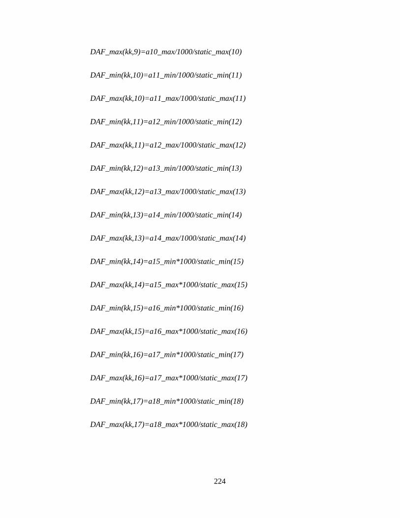
224
DAF_max(kk,9)=a10_max/1000/static_max(10)
DAF_min(kk,10)=a11_min/1000/static_min(11)
DAF_max(kk,10)=a11_max/1000/static_max(11)
DAF_min(kk,11)=a12_min/1000/static_min(12)
DAF_max(kk,11)=a12_max/1000/static_max(12)
DAF_min(kk,12)=a13_min/1000/static_min(13)
DAF_max(kk,12)=a13_max/1000/static_max(13)
DAF_min(kk,13)=a14_min/1000/static_min(14)
DAF_max(kk,13)=a14_max/1000/static_max(14)
DAF_min(kk,14)=a15_min*1000/static_min(15)
DAF_max(kk,14)=a15_max*1000/static_max(15)
DAF_min(kk,15)=a16_min*1000/static_min(16)
DAF_max(kk,15)=a16_max*1000/static_max(16)
DAF_min(kk,16)=a17_min*1000/static_min(17)
DAF_max(kk,16)=a17_max*1000/static_max(17)
DAF_min(kk,17)=a18_min*1000/static_min(18)
DAF_max(kk,17)=a18_max*1000/static_max(18)

225
*do,i,1,E_num+25 !save the time history into array parameters
uz_side(i,kk)=disp_side(i)*1000
uz_side_L(i,kk)=disp_side_L(i)*1000
uz_side_R(i,kk)=disp_side_R(i)*1000
uz_mid(i,kk)=disp_mid(i)*1000
uz_mid_L(i,kk)=disp_mid_L(i)*1000
uz_mid_R(i,kk)=disp_mid_R(i)*1000
fmx_side(i,kk)=mx_side(i)/1000
fmy_side(i,kk)=my_side(i)/1000
ffz_side(i,kk)=fz_side(i)/1000
fmx_zhi(i,kk)=mx_zhi(i)/1000
fmy_zhi(i,kk)=my_zhi(i)/1000
ffz_zhi(i,kk)=fz_zhi(i)/1000
fmx_mid(i,kk)=mx_mid(i)/1000
fmy_mid(i,kk)=my_mid(i)/1000

226
ffz_mid(i,kk)=fz_mid(i)/1000
fmz_dun(i,kk)=mz_dun(i)/1000
ffx_dun(i,kk)=fx_dun(i)/1000
*enddo
*enddo
*mWRITE,uz_side(1,1),uz_sideev0,txt,,jik,15,525
(15F10.5)
*mWRITE,uz_side_L(1,1),uz_side_Lev0,txt,,jik,15,525
(15F10.5)
*mWRITE,uz_side_R(1,1),uz_side_Rev0,txt,,jik,15,525
(15F10.5)
*mWRITE,uz_mid(1,1),uz_midev0,txt,,jik,15,525
(15F10.5)
*mWRITE,uz_mid_L(1,1),uz_mid_Lev0,txt,,jik,15,525
(15F10.5)
*mWRITE,uz_mid_R(1,1),uz_mid_Rev0,txt,,jik,15,525

227
(15F10.5)
*mWRITE,fmx_side(1,1),fmx_sideev0,txt,,jik,15,525
(15F15.3)
*mWRITE,fmy_side(1,1),fmy_sideev0,txt,,jik,15,525
(15F15.3)
*mWRITE,ffz_side(1,1),ffz_sideev0,txt,,jik,15,525
(15F15.3)
*mWRITE,fmx_zhi(1,1),fmx_zhiev0,txt,,jik,15,525
(15F15.3)
*mWRITE,fmy_zhi(1,1),fmy_zhiev0,txt,,jik,15,525
(15F15.3)
*mWRITE,ffz_zhi(1,1),ffz_zhiev0,txt,,jik,15,525
(15F15.3)
*mWRITE,fmx_mid(1,1),fmx_midev0,txt,,jik,15,525
(15F15.3)
*mWRITE,fmy_mid(1,1),fmy_midev0,txt,,jik,15,525
(15F15.3)

228
*mWRITE,ffz_mid(1,1),ffz_midev0,txt,,jik,15,525
(15F15.3)
*mWRITE,fmz_dun(1,1),fmz_dunev0,txt,,jik,15,525
(15F15.3)
*mWRITE,ffx_dun(1,1),ffx_dunev0,txt,,jik,15,525
(15F15.3)
*mWRITE,DAF_min(1,1),DAF_minev0,txt,,jik,18,15
(18F10.4)
*mWRITE,DAF_max(1,1),DAF_maxev0,txt,,jik,18,15
(18F10.4)
parsav,all,parameter_r2_ev0

229

230
11. Appendix – B
Code of Surface condition generator
Matlab
clear;
clc;
format short;
syms c k;
a=0.6;
b=0.5;
t=0.4;
v=0.3;
x=a./2.*c;
y=b./2.*k;
J=[a./2 0;0 b./2];
Y11=diff(y,k)./det(J);
Y12=-diff(y,c)./det(J);

231
Y21=-diff(x,k)./det(J);
Y22=diff(x,c)./det(J);
D=[Y11 Y12 0 0; 0 0 Y21 Y22; Y21 Y22 Y11 Y12];
N1=(1+c).*(1+k)./4;
N2=(1-c).*(1+k)./4;
N3=(1-c).*(1-k)./4;
N4=(1+c).*(1-k)./4;
N=[diff(N1,c) 0 diff(N2,c) 0 diff(N3,c) 0 diff(N3,c) 0; diff(N1,k) 0 diff(N2,k) 0
diff(N3,k) 0 diff(N3,k) 0; 0 diff(N1,c) 0 diff(N2,c) 0 diff(N3,c) 0 diff(N3,c); 0 diff(N1,k) 0
diff(N2,k) 0 diff(N3,k) 0 diff(N3,k)];
B=D*N;
C=(10.^7./(1-v.^2)).*[1 v 0; v 1 0; 0 0 (1-v)./2];
eK=B'*C*B.*t.*det(J);
k1=double(subs(eK,c,k,-1./sqrt(3),-1./sqrt(3)));
k2=double(subs(eK,c,k,-1./sqrt(3),1./sqrt(3)));
k3=double(subs(eK,c,k,1./sqrt(3),-1./sqrt(3)));
k4=double(subs(eK,c,k,1./sqrt(3),1./sqrt(3)));
eK=k1+k2+k3+k4;

232
Ty1=(1+c).*(1-(0.3.*c+5.7)./6);
Ty2=(1+c).*(1-(0.3.*c+5.1)./6);
Ty3=(1+c).*(1-(0.3.*c+4.5)./6);
Ty4=(1+c).*(1-(0.3.*c+3.9)./6);
Ty5=(1+c).*(1-(0.3.*c+3.3)./6);
Ty6=(1+c).*(1-(0.3.*c+2.7)./6);
Ty7=(1+c).*(1-(0.3.*c+2.1)./6);
Ty8=(1+c).*(1-(0.3.*c+1.5)./6);
Ty9=(1+c).*(1-(0.3.*c+0.9)./6);
Ty10=(1+c).*(1-(0.3.*c+0.3)./6);
C1=double(int(Ty1, c, -1, 1).*a.*t./4);
C2=double(int(Ty2, c, -1, 1).*a.*t./4);
C3=double(int(Ty3, c, -1, 1).*a.*t./4);
C4=double(int(Ty4, c, -1, 1).*a.*t./4);
C5=double(int(Ty5, c, -1, 1).*a.*t./4);
C6=double(int(Ty6, c, -1, 1).*a.*t./4);
C7=double(int(Ty7, c, -1, 1).*a.*t./4);

233
C8=double(int(Ty8, c, -1, 1).*a.*t./4);
C9=double(int(Ty9, c, -1, 1).*a.*t./4);
C10=double(int(Ty10, c, -1, 1).*a.*t./4);
T1=(1-c).*(1-(0.3.*c+5.7)./6);
T2=(1-c).*(1-(0.3.*c+5.1)./6);
T3=(1-c).*(1-(0.3.*c+4.5)./6);
T4=(1-c).*(1-(0.3.*c+3.9)./6);
T5=(1-c).*(1-(0.3.*c+3.3)./6);
T6=(1-c).*(1-(0.3.*c+2.7)./6);
T7=(1-c).*(1-(0.3.*c+2.1)./6);
T8=(1-c).*(1-(0.3.*c+1.5)./6);
T9=(1-c).*(1-(0.3.*c+0.9)./6);
T10=(1-c).*(1-(0.3.*c+0.3)./6);
D1=double(int(T1, c, -1, 1).*a.*t./4);
D2=double(int(T2, c, -1, 1).*a.*t./4);
D3=double(int(T3, c, -1, 1).*a.*t./4);
D4=double(int(T4, c, -1, 1).*a.*t./4);

234
D5=double(int(T5, c, -1, 1).*a.*t./4);
D6=double(int(T6, c, -1, 1).*a.*t./4);
D7=double(int(T7, c, -1, 1).*a.*t./4);
D8=double(int(T8, c, -1, 1).*a.*t./4);
D9=double(int(T9, c, -1, 1).*a.*t./4);
D10=double(int(T10, c, -1, 1).*a.*t./4);
F=[0; C1; 0; D1+C2; 0; D2+C3; 0; D3+C4; 0; D4+C5; 0; D5+C6; 0; D6+C7; 0;
D7+C8; 0; D8+C9; 0; D9+C10; 0; D10; 0; 0; 0; 0; 0; 0; 0; 0; 0; 0; 0; 0; 0; 0; 0; 0; 0;
0; 0; 0; 0; 0; 0; 0; 0; 0; 0; 0; 0; 0; 0; 0; 0; 0; 0; 0; 0; 0; 0; 0; 0; 0; 0; 0];
gK=zeros(66,66);
for i=1:2:41;
gK(i:i+3,i:i+3)=gK(i:i+3,i:i+3)+eK(1:4,1:4);
end
for i=23:2:63;
gK(i:i+3,i:i+3)=gK(i:i+3,i:i+3)+eK(5:8,5:8);
end
for i=1:2:41;
gK(i:i+3,i+22:i+25)=gK(i:i+3,i+22:i+25)+eK(1:4,5:8);

235
end
for i=1:2:41;
gK(i+22:i+25,i:i+3)=gK(i+22:i+25,i:i+3)+eK(5:8,1:4);
end
gKBC=zeros(60,60);
gKBC(1:20,1:20)=gK(1:20,1:20);
gKBC(1:20,21:40)=gK(1:20,23:42);
gKBC(1:20,41:60)=gK(1:20,45:64);
gKBC(21:40,1:20)=gK(23:42,1:20);
gKBC(21:40,21:40)=gK(23:42,23:42);
gKBC(21:40,41:60)=gK(23:42,45:64);
gKBC(41:60,1:20)=gK(45:64,1:20);
gKBC(41:60,21:40)=gK(45:64,23:42);
gKBC(41:60,41:60)=gK(45:64,45:64);
gFBC=zeros(60,1);
gFBC(1:20,1)=F(1:20,1);
gFBC(21:40,1)=F(23:42,1);

236
gFBC(41:60,1)=F(45:64,1);
q=inv(gKBC)*gFBC;
for i=1:30;
Q(i,1)=q(2*i,1);
end
for i=1:10;
Y(i,1)=Q(i,1)+Q(i+10,1)+Q(i+20,1);
end
j=max(Y);
h=1/j;
Z=h.*Y;
clc
hw8tryout
%-- 4/24/2013 1:21 PM --%
%-- 5/13/2013 11:39 PM --%
clear;
clc;

237
format short;
syms c k;
a=0.6;
b=0.5;
t=0.4;
v=0.3;
x=a./2.*c;
y=b./2.*k;
J=[a./2 0;0 b./2];
Y11=diff(y,k)./det(J);
Y12=-diff(y,c)./det(J);
Y21=-diff(x,k)./det(J);
Y22=diff(x,c)./det(J);
D=[Y11 Y12 0 0; 0 0 Y21 Y22; Y21 Y22 Y11 Y12];
N1=(1+c).*(1+k)./4;
N2=(1-c).*(1+k)./4;
N3=(1-c).*(1-k)./4;

238
N4=(1+c).*(1-k)./4;
N=[diff(N1,c) 0 diff(N2,c) 0 diff(N3,c) 0 diff(N3,c) 0; diff(N1,k) 0 diff(N2,k) 0
diff(N3,k) 0 diff(N3,k) 0; 0 diff(N1,c) 0 diff(N2,c) 0 diff(N3,c) 0 diff(N3,c); 0 diff(N1,k) 0
diff(N2,k) 0 diff(N3,k) 0 diff(N3,k)];
B=D*N;
C=(10.^7./(1-v.^2)).*[1 v 0; v 1 0; 0 0 (1-v)./2];
eK=B'*C*B.*t.*det(J);
k1=double(subs(eK,c,k,-1./sqrt(3),-1./sqrt(3)));
k2=double(subs(eK,c,k,-1./sqrt(3),1./sqrt(3)));
k3=double(subs(eK,c,k,1./sqrt(3),-1./sqrt(3)));
k4=double(subs(eK,c,k,1./sqrt(3),1./sqrt(3)));
eK=k1+k2+k3+k4;
Ty1=(1+c).*(1-(0.3.*c+5.7)./6);
Ty2=(1+c).*(1-(0.3.*c+5.1)./6);
Ty3=(1+c).*(1-(0.3.*c+4.5)./6);
Ty4=(1+c).*(1-(0.3.*c+3.9)./6);
Ty5=(1+c).*(1-(0.3.*c+3.3)./6);
Ty6=(1+c).*(1-(0.3.*c+2.7)./6);

239
Ty7=(1+c).*(1-(0.3.*c+2.1)./6);
Ty8=(1+c).*(1-(0.3.*c+1.5)./6);
Ty9=(1+c).*(1-(0.3.*c+0.9)./6);
Ty10=(1+c).*(1-(0.3.*c+0.3)./6);
C1=double(int(Ty1, c, -1, 1).*a.*t./4);
C2=double(int(Ty2, c, -1, 1).*a.*t./4);
C3=double(int(Ty3, c, -1, 1).*a.*t./4);
C4=double(int(Ty4, c, -1, 1).*a.*t./4);
C5=double(int(Ty5, c, -1, 1).*a.*t./4);
C6=double(int(Ty6, c, -1, 1).*a.*t./4);
C7=double(int(Ty7, c, -1, 1).*a.*t./4);
C8=double(int(Ty8, c, -1, 1).*a.*t./4);
C9=double(int(Ty9, c, -1, 1).*a.*t./4);
C10=double(int(Ty10, c, -1, 1).*a.*t./4);
T1=(1-c).*(1-(0.3.*c+5.7)./6);
T2=(1-c).*(1-(0.3.*c+5.1)./6);
T3=(1-c).*(1-(0.3.*c+4.5)./6);

240
T4=(1-c).*(1-(0.3.*c+3.9)./6);
T5=(1-c).*(1-(0.3.*c+3.3)./6);
T6=(1-c).*(1-(0.3.*c+2.7)./6);
T7=(1-c).*(1-(0.3.*c+2.1)./6);
T8=(1-c).*(1-(0.3.*c+1.5)./6);
T9=(1-c).*(1-(0.3.*c+0.9)./6);
T10=(1-c).*(1-(0.3.*c+0.3)./6);
D1=double(int(T1, c, -1, 1).*a.*t./4);
D2=double(int(T2, c, -1, 1).*a.*t./4);
D3=double(int(T3, c, -1, 1).*a.*t./4);
D4=double(int(T4, c, -1, 1).*a.*t./4);
D5=double(int(T5, c, -1, 1).*a.*t./4);
D6=double(int(T6, c, -1, 1).*a.*t./4);
D7=double(int(T7, c, -1, 1).*a.*t./4);
D8=double(int(T8, c, -1, 1).*a.*t./4);
D9=double(int(T9, c, -1, 1).*a.*t./4);
D10=double(int(T10, c, -1, 1).*a.*t./4);

241
F=[0; C1; 0; D1+C2; 0; D2+C3; 0; D3+C4; 0; D4+C5; 0; D5+C6; 0; D6+C7; 0;
D7+C8; 0; D8+C9; 0; D9+C10; 0; D10; 0; 0; 0; 0; 0; 0; 0; 0; 0; 0; 0; 0; 0; 0; 0; 0; 0;
0; 0; 0; 0; 0; 0; 0; 0; 0; 0; 0; 0; 0; 0; 0; 0; 0; 0; 0; 0; 0; 0; 0; 0; 0; 0; 0];
gK=zeros(66,66);
for i=1:2:41;
gK(i:i+3,i:i+3)=gK(i:i+3,i:i+3)+eK(1:4,1:4);
end
for i=23:2:63;
gK(i:i+3,i:i+3)=gK(i:i+3,i:i+3)+eK(5:8,5:8);
end
for i=1:2:41;
gK(i:i+3,i+22:i+25)=gK(i:i+3,i+22:i+25)+eK(1:4,5:8);
end
for i=1:2:41;
gK(i+22:i+25,i:i+3)=gK(i+22:i+25,i:i+3)+eK(5:8,1:4);
end
gKBC=zeros(60,60);
gKBC(1:20,1:20)=gK(1:20,1:20);

242
gKBC(1:20,21:40)=gK(1:20,23:42);
gKBC(1:20,41:60)=gK(1:20,45:64);
gKBC(21:40,1:20)=gK(23:42,1:20);
gKBC(21:40,21:40)=gK(23:42,23:42);
gKBC(21:40,41:60)=gK(23:42,45:64);
gKBC(41:60,1:20)=gK(45:64,1:20);
gKBC(41:60,21:40)=gK(45:64,23:42);
gKBC(41:60,41:60)=gK(45:64,45:64);
gFBC=zeros(60,1);
gFBC(1:20,1)=F(1:20,1);
gFBC(21:40,1)=F(23:42,1);
gFBC(41:60,1)=F(45:64,1);
q=inv(gKBC)*gFBC;
for i=1:30;
Q(i,1)=q(2*i,1);
end
for i=1:10;

243
Y(i,1)=Q(i,1)+Q(i+10,1)+Q(i+20,1);
end
j=max(Y);
h=1/j;
Z=h.*Y;
clc

244
12. Appendix -C
This appendix includes a sample of input files for analyzing and designing bridge
configuration using DESCUS II.
0101VM bridge long version
0102DESCUS Project
0103
0103 1 0 10 3 2 20.00 1 2
0301
0301 1 1 0.684 1 3 1 2 0.886 1 3 1 3 0.430 1 3
0301 1 4 0.000 1 3 1 5 0.000 1 3
0301 2 1 0.300 1 3 2 2 0.950 1 3 2 3 0.750 1 3
0301 2 4 0.000 1 3 2 5 0.000 1 3
0301 3 1 0.000 1 3 3 2 0.750 1 3 3 3 0.950 1 3
0301 3 4 0.300 1 3 3 5 0.000 1 3
0301 4 1 0.000 1 3 4 2 0.430 1 3 4 3 0.886 1 3
0301 4 4 0.684 1 3 4 5 0.000 1 3
0401

245
0401 4 8. 0 0 0 0 0 0
0402
04020 0 43.67 2. 2. 1. 1. 24. 8. 4. 150.
0403
0403 HL 93 1 1
0501
0501 1 1 5014. 71. 0.56 10. 1.0 84. 0.75 0.075 4.874
0501 3 1
0501 4 1 5014. 71. 0.56 10. 2.25 84. 1.5 0.075 4.874
0501 5 1 5014. 71. 0.56 13. 4.4 84. 3.0 0.075 4.874
0502
0502 2 1000. 1000.
0503
0503 1250. 0 0
0601
0601 1 0.000 0.0000 1 98 232 320
0601 2 0.000 10.8370 2 96 227 317

246
0601 3 0.000 22.0000 3 93 218 311
0601 4 0.000 10.8400 4 91 213 305
0602
060216. 25. 16.
0701
0701 1 1 8 10.35564 3 -635.8370 8 12 10.35565 3 -635.8370
0701 1 12 16 10.35565 3 -635.8370 16 20 10.35565 3 -635.8370
0701 1 20 24 10.35565 3 -635.8370 24 28 10.35565 3 -635.8370
0701 1 28 32 10.35565 3 -635.8370 32 36 10.35565 3 -635.8370
0701 1 36 40 10.35565 3 -635.8370 40 44 10.35565 3 -635.8370
0701 1 44 48 10.35565 3 -635.8370 48 52 10.35565 3 -635.8370
0701 1 52 56 10.35565 3 -635.8370 56 61 10.35565 3 -635.8370
0701 1 61 65 10.35565 3 -635.8370 65 69 10.35565 3 -635.8370
0701 1 69 73 10.35565 3 -635.8370 73 77 10.35565 3 -635.8370
0701 1 77 82 10.35565 3 -635.8370 82 86 10.35565 3 -635.8370
0701 1 86 90 10.35565 3 -635.8370 90 94 10.35565 3 -635.8370
0701 1 94 98 10.35566 3 -635.8370 98 102 10.35564 3 -635.8370

247
0701 1 102 106 10.35565 3 -635.8370 106 110 10.35565 3 -635.8370
0701 1 110 114 10.35565 3 -635.8370 114 119 10.35565 3 -635.8370
0701 1 119 123 10.35565 3 -635.8370 123 127 10.35565 3 -635.8370
0701 1 127 131 10.35565 3 -635.8370 131 135 10.35565 3 -635.8370
0701 1 135 139 10.35565 3 -635.8370 139 143 10.35565 3 -635.8370
0701 1 143 147 10.35565 3 -635.8370 147 151 10.35565 3 -635.8370
0701 1 151 156 10.35565 3 -635.8370 156 160 10.35565 3 -635.8370
0701 1 160 164 10.35565 3 -635.8370 164 168 10.35565 3 -635.8370
0701 1 168 173 10.35565 3 -635.8370 173 177 10.35565 3 -635.8370
0701 1 177 181 10.35565 3 -635.8370 181 185 10.35565 3 -635.8370
0701 1 185 189 10.35565 3 -635.8370 189 193 10.35565 3 -635.8370
0701 1 193 197 10.35565 3 -635.8370 197 201 10.35565 3 -635.8370
0701 1 201 205 10.35565 3 -635.8370 205 209 10.35565 3 -635.8370
0701 1 209 214 10.35565 3 -635.8370 214 219 10.35565 3 -635.8370
0701 1 219 223 10.35565 3 -635.8370 223 228 10.35565 3 -635.8370
0701 1 228 232 1.03557 3 -635.8370 232 234 9.32008 3 -635.8370
0701 1 234 239 10.35565 3 -635.8370 239 243 10.35565 3 -635.8370

248
0701 1 243 248 10.35565 3 -635.8370 248 252 10.35565 3 -635.8370
0701 1 252 256 10.35565 3 -635.8370 256 260 10.35565 3 -635.8370
0701 1 260 264 10.35565 3 -635.8370 264 268 10.35565 3 -635.8370
0701 1 268 272 10.35565 3 -635.8370 272 276 10.35565 3 -635.8370
0701 1 276 280 10.35565 3 -635.8370 280 284 10.35565 3 -635.8370
0701 1 284 289 10.35565 3 -635.8370 289 293 10.35565 3 -635.8370
0701 1 293 297 10.35565 3 -635.8370 297 301 10.35565 3 -635.8370
0701 1 301 306 10.35565 3 -635.8370 306 309 10.35565 3 -635.8370
0701 1 309 313 10.35565 3 -635.8370 313 315 10.35565 3 -635.8370
0701 1 315 318 10.35565 3 -635.8370 318 319 10.35565 3 -635.8370
0701 1 319 320 1.03557 3 -635.8370
0701 2 2 7 10.17915 1 -625.0000 7 11 10.17915 1 -625.0000
0701 2 11 15 10.17915 1 -625.0000 15 19 10.17915 4 -625.0000
0701 2 19 23 10.17915 4 -625.0000 23 27 10.17915 4 -625.0000
0701 2 27 31 10.17915 4 -625.0000 31 35 10.17915 4 -625.0000
0701 2 35 39 10.17915 4 -625.0000 39 43 10.17915 4 -625.0000
0701 2 43 47 10.17915 4 -625.0000 47 51 10.17915 4 -625.0000

249
0701 2 51 55 10.17915 4 -625.0000 55 59 10.17915 4 -625.0000
0701 2 59 63 10.17915 4 -625.0000 63 67 10.17915 4 -625.0000
0701 2 67 71 10.17915 4 -625.0000 71 75 10.17915 4 -625.0000
0701 2 75 80 10.17915 5 -625.0000 80 84 10.17915 5 -625.0000
0701 2 84 88 10.17915 5 -625.0000 88 92 10.17915 5 -625.0000
0701 2 92 96 10.17916 5 -625.0000 96 100 10.17915 5 -625.0000
0701 2 100 104 10.17915 5 -625.0000 104 108 10.17915 5 -625.0000
0701 2 108 112 10.17915 5 -625.0000 112 117 10.17915 5 -625.0000
0701 2 117 121 10.17915 4 -625.0000 121 125 10.17915 4 -625.0000
0701 2 125 129 10.17915 4 -625.0000 129 133 10.17915 4 -625.0000
0701 2 133 137 10.17915 4 -625.0000 137 141 10.17915 4 -625.0000
0701 2 141 145 10.17915 4 -625.0000 145 149 10.17915 4 -625.0000
0701 2 149 154 10.17915 4 -625.0000 154 158 10.17915 4 -625.0000
0701 2 158 162 10.17915 4 -625.0000 162 166 10.17915 4 -625.0000
0701 2 166 170 10.17915 4 -625.0000 170 174 10.17915 4 -625.0000
0701 2 174 178 10.17915 5 -625.0000 178 182 10.17915 5 -625.0000
0701 2 182 186 10.17915 5 -625.0000 186 190 10.17915 5 -625.0000

250
0701 2 190 194 10.17915 5 -625.0000 194 198 10.17915 5 -625.0000
0701 2 198 202 10.17915 5 -625.0000 202 206 10.17915 5 -625.0000
0701 2 206 210 10.17915 5 -625.0000 210 215 10.17915 5 -625.0000
0701 2 215 220 10.17915 5 -625.0000 220 224 10.17915 5 -625.0000
0701 2 224 227 1.01792 5 -625.0000 227 231 9.16123 5 -625.0000
0701 2 231 236 10.17915 5 -625.0000 236 240 10.17915 5 -625.0000
0701 2 240 244 10.17915 5 -625.0000 244 247 10.17915 5 -625.0000
0701 2 247 251 10.17915 4 -625.0000 251 255 10.17915 4 -625.0000
0701 2 255 259 10.17915 4 -625.0000 259 263 10.17915 4 -625.0000
0701 2 263 267 10.17915 4 -625.0000 267 271 10.17915 4 -625.0000
0701 2 271 275 10.17915 4 -625.0000 275 279 10.17915 4 -625.0000
0701 2 279 283 10.17915 4 -625.0000 283 287 10.17915 4 -625.0000
0701 2 287 291 10.17915 4 -625.0000 291 295 10.17915 4 -625.0000
0701 2 295 299 10.17915 4 -625.0000 299 304 10.17915 4 -625.0000
0701 2 304 308 10.17915 4 -625.0000 308 312 10.17915 4 -625.0000
0701 2 312 314 10.17915 1 -625.0000 314 316 10.17915 1 -625.0000
0701 2 316 317 1.01792 1 -625.0000
251
0701 3 3 6 9.82085 1 -603.0000 6 10 9.82085 1 -603.0000
0701 3 10 14 9.82085 1 -603.0000 14 18 9.82085 4 -603.0000
0701 3 18 22 9.82085 4 -603.0000 22 26 9.82085 4 -603.0000
0701 3 26 30 9.82085 4 -603.0000 30 34 9.82085 4 -603.0000
0701 3 34 38 9.82085 4 -603.0000 38 42 9.82085 4 -603.0000
0701 3 42 46 9.82085 4 -603.0000 46 50 9.82085 4 -603.0000
0701 3 50 54 9.82085 4 -603.0000 54 58 9.82085 4 -603.0000
0701 3 58 62 9.82085 4 -603.0000 62 66 9.82085 4 -603.0000
0701 3 66 70 9.82085 4 -603.0000 70 74 9.82085 4 -603.0000
0701 3 74 78 9.82085 5 -603.0000 78 81 9.82085 5 -603.0000
0701 3 81 85 9.82085 5 -603.0000 85 89 9.82085 5 -603.0000
0701 3 89 93 9.82084 5 -603.0000 93 97 9.82085 5 -603.0000
0701 3 97 101 9.82085 5 -603.0000 101 105 9.82085 5 -603.0000
0701 3 105 109 9.82085 5 -603.0000 109 113 9.82085 5 -603.0000
0701 3 113 116 9.82085 5 -603.0000 116 120 9.82085 5 -603.0000
0701 3 120 124 9.82085 4 -603.0000 124 128 9.82085 4 -603.0000
0701 3 128 132 9.82085 4 -603.0000 132 136 9.82085 4 -603.0000

252
0701 3 136 140 9.82085 4 -603.0000 140 144 9.82085 4 -603.0000
0701 3 144 148 9.82085 4 -603.0000 148 152 9.82085 4 -603.0000
0701 3 152 155 9.82085 4 -603.0000 155 159 9.82085 4 -603.0000
0701 3 159 163 9.82085 4 -603.0000 163 167 9.82085 4 -603.0000
0701 3 167 171 9.82085 4 -603.0000 171 175 9.82085 4 -603.0000
0701 3 175 179 9.82085 5 -603.0000 179 183 9.82085 5 -603.0000
0701 3 183 187 9.82085 5 -603.0000 187 191 9.82085 5 -603.0000
0701 3 191 195 9.82085 5 -603.0000 195 199 9.82085 5 -603.0000
0701 3 199 203 9.82085 5 -603.0000 203 207 9.82085 5 -603.0000
0701 3 207 211 9.82085 5 -603.0000 211 216 9.82085 5 -603.0000
0701 3 216 218 0.98208 5 -603.0000 218 222 8.83877 5 -603.0000
0701 3 222 226 9.82085 5 -603.0000 226 230 9.82085 5 -603.0000
0701 3 230 235 9.82085 5 -603.0000 235 238 9.82085 4 -603.0000
0701 3 238 242 9.82085 4 -603.0000 242 246 9.82085 4 -603.0000
0701 3 246 250 9.82085 4 -603.0000 250 254 9.82085 4 -603.0000
0701 3 254 258 9.82085 4 -603.0000 258 262 9.82085 4 -603.0000
0701 3 262 266 9.82085 4 -603.0000 266 270 9.82085 4 -603.0000

253
0701 3 270 274 9.82085 4 -603.0000 274 278 9.82085 4 -603.0000
0701 3 278 282 9.82085 4 -603.0000 282 286 9.82085 4 -603.0000
0701 3 286 290 9.82085 4 -603.0000 290 294 9.82085 4 -603.0000
0701 3 294 298 9.82085 4 -603.0000 298 302 9.82085 4 -603.0000
0701 3 302 307 9.82085 1 -603.0000 307 310 9.82085 1 -603.0000
0701 3 310 311 0.98208 1 -603.0000
0701 4 4 5 9.64431 3 -592.1600 5 9 9.64430 3 -592.1600
0701 4 9 13 9.64430 3 -592.1600 13 17 9.64430 3 -592.1600
0701 4 17 21 9.64430 3 -592.1600 21 25 9.64430 3 -592.1600
0701 4 25 29 9.64430 3 -592.1600 29 33 9.64430 3 -592.1600
0701 4 33 37 9.64430 3 -592.1600 37 41 9.64430 3 -592.1600
0701 4 41 45 9.64430 3 -592.1600 45 49 9.64430 3 -592.1600
0701 4 49 53 9.64430 3 -592.1600 53 57 9.64430 3 -592.1600
0701 4 57 60 9.64430 3 -592.1600 60 64 9.64430 3 -592.1600
0701 4 64 68 9.64430 3 -592.1600 68 72 9.64430 3 -592.1600
0701 4 72 76 9.64430 3 -592.1600 76 79 9.64430 3 -592.1600
0701 4 79 83 9.64430 3 -592.1600 83 87 9.64430 3 -592.1600

254
0701 4 87 91 9.64429 3 -592.1600 91 95 9.64431 3 -592.1600
0701 4 95 99 9.64430 3 -592.1600 99 103 9.64430 3 -592.1600
0701 4 103 107 9.64430 3 -592.1600 107 111 9.64430 3 -592.1600
0701 4 111 115 9.64430 3 -592.1600 115 118 9.64430 3 -592.1600
0701 4 118 122 9.64430 3 -592.1600 122 126 9.64430 3 -592.1600
0701 4 126 130 9.64430 3 -592.1600 130 134 9.64430 3 -592.1600
0701 4 134 138 9.64430 3 -592.1600 138 142 9.64430 3 -592.1600
0701 4 142 146 9.64430 3 -592.1600 146 150 9.64430 3 -592.1600
0701 4 150 153 9.64430 3 -592.1600 153 157 9.64430 3 -592.1600
0701 4 157 161 9.64430 3 -592.1600 161 165 9.64430 3 -592.1600
0701 4 165 169 9.64430 3 -592.1600 169 172 9.64430 3 -592.1600
0701 4 172 176 9.64430 3 -592.1600 176 180 9.64430 3 -592.1600
0701 4 180 184 9.64430 3 -592.1600 184 188 9.64430 3 -592.1600
0701 4 188 192 9.64430 3 -592.1600 192 196 9.64430 3 -592.1600
0701 4 196 200 9.64430 3 -592.1600 200 204 9.64430 3 -592.1600
0701 4 204 208 9.64430 3 -592.1600 208 212 9.64430 3 -592.1600
0701 4 212 213 0.96442 3 -592.1600 213 217 8.67988 3 -592.1600

255
0701 4 217 221 9.64430 3 -592.1600 221 225 9.64430 3 -592.1600
0701 4 225 229 9.64430 3 -592.1600 229 233 9.64430 3 -592.1600
0701 4 233 237 9.64430 3 -592.1600 237 241 9.64430 3 -592.1600
0701 4 241 245 9.64430 3 -592.1600 245 249 9.64430 3 -592.1600
0701 4 249 253 9.64430 3 -592.1600 253 257 9.64430 3 -592.1600
0701 4 257 261 9.64430 3 -592.1600 261 265 9.64430 3 -592.1600
0701 4 265 269 9.64430 3 -592.1600 269 273 9.64430 3 -592.1600
0701 4 273 277 9.64430 3 -592.1600 277 281 9.64430 3 -592.1600
0701 4 281 285 9.64430 3 -592.1600 285 288 9.64430 3 -592.1600
0701 4 288 292 9.64430 3 -592.1600 292 296 9.64430 3 -592.1600
0701 4 296 300 9.64430 3 -592.1600 300 303 9.64430 3 -592.1600
0701 4 303 305 0.96442 3 -592.1600
0801
0801 1 1 2 2 2 2 3 2 3 3 4 2 4 8 7 2 5 7 6 2
0801 6 6 5 2 7 12 11 2 8 11 10 2 9 10 9 2 10 16 15 2
0801 11 15 14 2 12 14 13 2 13 20 19 2 14 19 18 2 15 18 17 2
0801 16 24 23 2 17 23 22 2 18 22 21 2 19 28 27 2 20 27 26 2

256
0801 21 26 25 2 22 32 31 2 23 31 30 2 24 30 29 2 25 36 35 2
0801 26 35 34 2 27 34 33 2 28 40 39 2 29 39 38 2 30 38 37 2
0801 31 44 43 2 32 43 42 2 33 42 41 2 34 48 47 2 35 47 46 2
0801 36 46 45 2 37 52 51 2 38 51 50 2 39 50 49 2 40 56 55 2
0801 41 55 54 2 42 54 53 2 43 61 59 2 44 59 58 2 45 58 57 2
0801 46 65 63 2 47 63 62 2 48 62 60 2 49 69 67 2 50 67 66 2
0801 51 66 64 2 52 73 71 2 53 71 70 2 54 70 68 2 55 77 75 2
0801 56 75 74 2 57 74 72 2 58 82 80 2 59 80 78 2 60 78 76 2
0801 61 86 84 2 62 84 81 2 63 81 79 2 64 90 88 2 65 88 85 2
0801 66 85 83 2 67 94 92 2 68 92 89 2 69 89 87 2 70 98 96 2
0801 71 96 93 2 72 93 91 2 73 102 100 2 74 100 97 2 75 97 95 2
0801 76 106 104 2 77 104 101 2 78 101 99 2 79 110 108 2 80 108 105 2
0801 81 105 103 2 82 114 112 2 83 112 109 2 84 109 107 2 85 119 117 2
0801 86 117 113 2 87 113 111 2 88 123 121 2 89 121 116 2 90 116 115 2
0801 91 127 125 2 92 125 120 2 93 120 118 2 94 131 129 2 95 129 124 2
0801 96 124 122 2 97 135 133 2 98 133 128 2 99 128 126 2 100 139 137 2
0801 101 137 132 2 102 132 130 2 103 143 141 2 104 141 136 2 105 136 134 2

257
0801 106 147 145 2 107 145 140 2 108 140 138 2 109 151 149 2 110 149 144 2
0801 111 144 142 2 112 156 154 2 113 154 148 2 114 148 146 2 115 160 158 2
0801 116 158 152 2 117 152 150 2 118 164 162 2 119 162 155 2 120 155 153 2
0801 121 168 166 2 122 166 159 2 123 159 157 2 124 173 170 2 125 170 163 2
0801 126 163 161 2 127 177 174 2 128 174 167 2 129 167 165 2 130 181 178 2
0801 131 178 171 2 132 171 169 2 133 185 182 2 134 182 175 2 135 175 172 2
0801 136 189 186 2 137 186 179 2 138 179 176 2 139 193 190 2 140 190 183 2
0801 141 183 180 2 142 197 194 2 143 194 187 2 144 187 184 2 145 201 198 2
0801 146 198 191 2 147 191 188 2 148 205 202 2 149 202 195 2 150 195 192 2
0801 151 209 206 2 152 206 199 2 153 199 196 2 154 214 210 2 155 210 203 2
0801 156 203 200 2 157 219 215 2 158 215 207 2 159 207 204 2 160 223 220 2
0801 161 220 211 2 162 211 208 2 163 228 224 2 164 224 216 2 165 216 212 2
0801 166 234 231 2 167 231 222 2 168 222 217 2 169 239 236 2 170 236 226 2
0801 171 226 221 2 172 243 240 2 173 240 230 2 174 230 225 2 175 248 244 2
0801 176 244 235 2 177 235 229 2 178 252 247 2 179 247 238 2 180 238 233 2
0801 181 256 251 2 182 251 242 2 183 242 237 2 184 260 255 2 185 255 246 2
0801 186 246 241 2 187 264 259 2 188 259 250 2 189 250 245 2 190 268 263 2

258
0801 191 263 254 2 192 254 249 2 193 272 267 2 194 267 258 2 195 258 253 2
0801 196 276 271 2 197 271 262 2 198 262 257 2 199 280 275 2 200 275 266 2
0801 201 266 261 2 202 284 279 2 203 279 270 2 204 270 265 2 205 289 283 2
0801 206 283 274 2 207 274 269 2 208 293 287 2 209 287 278 2 210 278 273 2
0801 211 297 291 2 212 291 282 2 213 282 277 2 214 301 295 2 215 295 286 2
0801 216 286 281 2 217 306 299 2 218 299 290 2 219 290 285 2 220 309 304 2
0801 221 304 294 2 222 294 288 2 223 313 308 2 224 308 298 2 225 298 292 2
0801 226 315 312 2 227 312 302 2 228 302 296 2 229 318 314 2 230 314 307 2
0801 231 307 300 2 232 319 316 2 233 316 310 2 234 310 303 2

259
13. Reference
AASHTO (2014). Load Resistance and Factor Design: Bridge Design
Specifications, Seventh Edition, American Association of State Highway and
Transportation Officials, Washington D.C.
AASHTO (2017). Load Resistance and Factor Design: Bridge Design
Specifications, Eighth Edition, American Association of State Highway and
Transportation Officials, Washington D.C.
Y.B. Yang, J.D. Yau, Y.S. Wu (2004), “Vehicle-Bridge Interaction Dynamics With
Applications to High-Speed Railways”, World Scientific Publishing Co.
Hu Ding, Kang Li Shi, Li Qun Chen and Shao Pu Yang (2013), “Dynamic response
of an infinite Timoshenko beam on a nonlinear viscoelastic foundation to a moving
load”, Nonlinear Dynamic 2013, 73: 285-298
L. Ma, W. Zhang, W.S. Han and J.X.Liu (2019) “Determining the dynamic
amplification factor of multi-span continuous box girder bridges in highways using
vehicle-bridge interaction analyses”, Engineering Structure, vol.181: 47-59
Cai C.B, He Q.L. and Zhu S.Y (2018), “Dynamic interaction of suspension-type
monorail vehicle and bridge: Numerical simulation and experiment”, Mechanical
Systems and Signal Processing, vol.118: 388-407

260
Zeng Q., Yang Y.B. and Elias G. (2016), “Dynamic response of high speed vehicles
and sustaining curved bridges under conditions of resonance”, Engineering Structure,
vol. 114: 61-74
Zhou S.H., Song G.Q., Wang R.P., Wen B.C. and Ren Z.H (2017), “Nonlinear
dynamic analysis for coupled vehicle-bridge vibration system on nonlinear foundation”,
Mechanical Systems and Signal Processing, vol. 87: 259-278
Arshad Mehmood, Ahmad Ali Khan et (2014), “Vibration Analysis of Beam
Subjected to Moving Loads Using Finite Element Method”, IOSR Journal of Engineering
2014 Vol 04 issue 5
M.Ichikawa, Y.Miyakawa, A.Matsuda (2000), “Vibration Analysis of the continuous
Beam Subjected to a Moving Mass”, Journal of Sound and Vibration 2000 vol. 230 issue
3:493-506
S,Eftekhar Azam, M.Mofid, R.Afghani Khorasknai (2012),”Dyanamic response of
Timoshenko beam under moving mass”, Scientia Iranica 2013 vol.20 issue 1
AV Pesterev, LA Bergman (2000), “Am improved series expansion of the solution to
the moving oscillator problem”, Journal of Vibration and Acoustics, Transactions of the
ASME 2000 Jan 1:54-61
AV Pesterev, LA Bergman (2001), “Response of elastic continuum carrying multiple
moving oscillators”, Journal of engineering mechanics 127 issue 3:260-265
261
Mario Fafard, Mallikarjuna Bennur (1996), “A general multi-axle vehicle model to
study the bridge-vehicle interaction” Engineering Computations 14 issue 5:491-508
Gupta R.K. (1980),”Dynamic loading of highway bridges”, Journal of Engineering
Mechanics 106 issue 2: 377-397
Ton-Lo Wang, Dongzhou Huang et al. (1996),”Dynamic Behavior of Continuous
and Cantilever Thin-walled Box Girder Bridges”, Journal of Bridge Engineering 1996
Vol.1 issue 2
Wu J.S. and Dai C.W. (1987), “Dynamic responses of multispan nonuniform beam
due to moving loads”, Journal of Structural Engineering ASCE 113 issue 3:458-474
Marchesiello S, Fasana A, Garibaldi L and Piombo, (1999) “Dynamics of multi-
span continuous straight bridges subject to multi-degrees of freedom moving vehicle
excitation” Journal of Sound and Vibration 224 issue 3: 541-561
Yang Y.B., Liao S.S. and Lin B.H. (1995) “Impact formulas for vehicles moving over
simple and continuous beams”, Journal of Structural Engineering ASCE 121 issue 11:
1644-1650
Paultre P., Chaallal O. and Proulx J. (1992), ”Bridge dynamics and dynamic
amplification factors – A review of analytical experimental findings” Canadian Journal
Civil Engineering vol.19: 260-278
Huang E.S. and Nowak A.S. (1991), “Simulation of dynamic load for bridges”,
Journal of Structural Engineering ASCE, vol.117 issue 5: 1413-1434

262
Chang D. and Lee H. (1994), “Impact factors for simple-span highway girder
bridges”, Journal of Structure Engineering ASCE vol.120 issue 3: 704-715
Dodds C.J. and Robson J.D. (1973), “The description of road surface roughness”,
Journal of Sound and Vibration vol.31 issue 2: 175-183
Marcondes J, Burgess G.J., Harichandran R. and Snyder M.B. (1991),”Spectral
analysis of highway pavement roughness”, Journal of Transportation Engineering ASCE,
vol.117 issue 5: 540-549
Tan C.P. and Shore S. (1968), “Dynamic response of a horizontally curved bridge”,
Journal of Structural Division ASCE, vol. 94 issue 3: 761-781
Tan C.P. and Shore S. (1968), “Response of horizontally curved bridges to moving
load”, Journal of Structural Division ASCE, vol. 94 issue 9: 2135-2151
Yang Y.B., Wu C.M. AND Yau J.D. (2001), “Dynamic response of a horizontally
curved beam subjected to vertical and horizontal moving loads”, Journal of Sound and
Vibration vol.243 issue 3: 519-537
Song Y.F. and He S.H. (2001), “Study on Key Response Factors for Impact Force
Withstood by Highway Bridge”, Journal of Xi’an Highway University, vol.21 issue 2: 47-
49
M. Maijka and Michael Hartnett (2008), “ Effects of speed, load and damping on
the dynamic response of railway bridges and vehicles”, Computers & Structures vol. 86,
issue 6: 556-572

263
Chunhua Liu, Dongzhou Huang, Ton-Lo Wang (2002), “Analytical dynamic impact
study based on correlated road roughness”, Computers and Structures 2002 vol.80:
1639–1650
Ton-Lo Wang and Dongzhou Huang (1992), Cable-Stayed Bridge Vibration Due To
Road Surface Roughness, Journal of Structural Engineering, Vol. 118
Mohammad Al-Emrani (2005),“Fatigue Performance of Stringer-to-Floor-Beam
Connections in Riveted Railway Bridges”, ASCE_1084-0702_2005_10:2_179
Khaled M. Sennah, Xuesheng Zhang, and John B. Kennedy (2004) “Impact Factors
for Horizontally Curved Composite Box Girder Bridges”, ASCE_1084-
0702_2004_9:6_512
Dongzhou Huang (2005), “Dynamic Analysis of Steel Curved Box Girder Bridges”,
Journal of Bridge Engineering 2005.
Ton-Lo Wang, Dongzhou Huang, Mohsen Shahawy and Kaizan Huang
(1995),”Dynamic response of Highway Girder Bridges”, Computers & Structures Vol
60: 1021-1027
Hid N. Grouni, Andrze S. Nowak (1984), “Calibration of the Ontario Bridge Design
Code 1983 edition”, Canadian journal of civil engineering 1984. 11: 760-770.
Hid N. Grouni, Andrze S. Nowak (1993), ”Calibration of the Ontario Highway
Bridge Design Code 1991 edition”, Canadian journal of civil engineering 1994.21: 25-
35.

264
Dongzhou Huang, Ton-Lo Wang and Mohsen Shahawy (1993), “Impact Analysis of
Continuous Multi-girder Bridges due to Moving Vehicles” Journal of Structural
Engineering, vol.118: 2953
Dongzhou Huang, Ton-Lo Wang, M. Shahawy (1997), “Vibration of horizontally
curved box girder bridges due to vehicles”, Computers & Structures, vol 68: 513-528
Hongyi Li (2005), “Dynamic Response Of Highway Bridge Subjected To Heavy
Vehicles”, The Florida State University, FAMU-FSU College of Engineering.
CSI. CSiBridge 2017. Berkeley, CA: Computers and Structures, Inc.
Kalny, O., (2015). CSI Knowledge Base, Internet:
https://wiki.csiamerica.com/display/kb/Home.
Fu, C. C. (2009). DESCUS II. Win-DESCUS User's manual for Design and Analysis
of Curved BOX-Girder Bridge Systems, 12. College Park, MD: The BEST Center,
University of Maryland.