
ABSTRACT Title of Dissertation: EXPERIMENTAL ... - DRUM
211
ABSTRACT Title of Dissertation: EXPERIMENTAL VALIDATION OF TRAC-RELAP ADVANCED COMPUTATIONAL ENGINE (TRACE) FOR SIMPLIFIED, INTEGRAL, RAPID- CONDENSATION-DRIVEN TRANSIENT Anthony Gerard Pollman, Doctor of Philosophy, 2011 Dissertation directed by: Professor Marino di Marzo Department of Fire Protection Engineering The purpose of the present work is to experimentally validate the TRACE (TRAC-RELAP Advanced Computational Engine) plug-in of the Nuclear Regulatory Commission’s (NRC’s) Symbolic Nuclear Analysis Package (SNAP) for rapid condensation transients. These transients are challenging for the code. The experimental phase began by constructing and calibrating a simplified, integral, condensation-driven transient apparatus named the UMD-USNA Near One- dimensional Transient Experimental Assembly (MANOTEA). Then, a series of 5 well- defined transients were run. Data from the facility included: pressure, differential pressure, and temperature, all as a function of time. Using the data, mass and energy balances were closed for each experiment. Some of the relevant characteristics of the data included: inverted thermal stratification and nozzle dependent transients controlled by an energy partition. A common transient sequence was identified and served as the fundamental comparison to evaluate TRACE.
Transcript of ABSTRACT Title of Dissertation: EXPERIMENTAL ... - DRUM

ABSTRACT
Title of Dissertation: EXPERIMENTAL VALIDATION OF TRAC-RELAP ADVANCED COMPUTATIONAL ENGINE (TRACE) FOR SIMPLIFIED, INTEGRAL, RAPID-CONDENSATION-DRIVEN TRANSIENT
Anthony Gerard Pollman, Doctor of Philosophy, 2011 Dissertation directed by: Professor Marino di Marzo Department of Fire Protection Engineering
The purpose of the present work is to experimentally validate the TRACE
(TRAC-RELAP Advanced Computational Engine) plug-in of the Nuclear Regulatory
Commission’s (NRC’s) Symbolic Nuclear Analysis Package (SNAP) for rapid
condensation transients. These transients are challenging for the code.
The experimental phase began by constructing and calibrating a simplified,
integral, condensation-driven transient apparatus named the UMD-USNA Near One-
dimensional Transient Experimental Assembly (MANOTEA). Then, a series of 5 well-
defined transients were run. Data from the facility included: pressure, differential
pressure, and temperature, all as a function of time. Using the data, mass and energy
balances were closed for each experiment. Some of the relevant characteristics of the
data included: inverted thermal stratification and nozzle dependent transients controlled
by an energy partition. A common transient sequence was identified and served as the
fundamental comparison to evaluate TRACE.

The second phase began by developing a 1-dimensional Base TRACE Model.
Output from the Base Model was found to over-estimate the pressures and temperatures
observed in the experiment. This Model always predicted that the condenser pipe would
fill, and that transients would terminate with a non-physical discontinuity. In an effort to
improve the model, a list of phenomena was generated and then mapped to TRACE
parameters. The goal was to find unique ways to capture the energy partition and prevent
the condenser from filling. Over 250 TRACE cases were run, and the effective and
physically justifiable parameters were incorporated into a 3-dimensional Final TRACE
Model. The Final Model incorporated non-condensable gases, which provided a
mechanism to terminate the transients smoothly. Replacing the PIPE component with a
VESSEL component provided a way to model the energy partition. The Final Model
under-predicted trends observed in the experiments. Thus, the two models were able to
bracket the experimental data.
Comparing TRACE output to the data led to the conclusion that the code’s
condensation model is over-stated. TRACE’s predecessors were also known to have
over-stated condensation models. As a result, TRACE will over-predict condensation-
induced fluid motion when modeling several thermal-hydraulic situations important to
safe nuclear reactor operation. Future work could focus on developing a NOZZLE
component for TRACE, comparing the subsequent output to MANOTEA data and
improving the TRACE condensation model.

EXPERIMENTAL VALIDATION OF TRAC-RELAP ADVANCED COMPUTATIONAL ENGINE (TRACE) FOR SIMPLIFIED, INTEGRAL, RAPID-
CONDENSATION-DRIVEN TRANSIENT
by
Anthony Gerard Pollman.
Dissertation submitted to the Faculty of the Graduate School of the University of Maryland, College Park, in partial fulfillment
of the requirements for the degree of Doctor of Philosophy
2011 Advisory Committee: Doctor Marino di Marzo, Chair Doctor Karen Vierow Doctor Amr Baz Doctor Ken Kiger Doctor Gary Pertmer, Dean’s Representative

© Copyright by
Anthony Gerard Pollman
2011

ii
TABLE OF CONTENTS List of Tables……………………………………………………………………………..vi List of Figures……………………………………………………………………………vii List of Symbols…………………………………………………………………………...xi Chapter 1: Introduction……………………………………………………………………1 Significance of Present Study……………………………………………………..1 Approach and Objectives………………………………………………………….1 Dissertation Organization…………………………………………………………2 Chapter 2: Literature Review……………………………………………………………...3 Integral Transients………………………………………………………………...3 Rapid Condensation……………………………………………………………….4 Rapid Condensation in Generation III+ Reactors…………………………4 Westinghouse AP1000…………………………………………….5 General Electric ESBW…………………………………………...6 Integral Experiments and Code Development…………………………………….6 PART 1: EXPERIMENT Chapter 3: Facility Description…………………………………………………………..10 Apparatus………………………………………………………………………...10 Facility Operation………………………………………………………………..13

iii
Facility Parameters Discussion…………………………………………………..17 Pressure…………………………………………………………………..17 Temperature……………………………………………………………...17 Initial Liquid Inventory…………………………………………………..18 Nozzle Geometry………………………………………………………...19 Operating Domains………………………………………………………………20 Chapter 4: Instrumentation………………………………………………………………22 Differential Pressure Cell…………………………………………………….…..22 Buoyant Rod Apparatus……………………………………………….…23 Drain Curves………………………………………………………….….25 Thermocouples…………………………………………………………………...26 Pressure Transducer……………………………………………………………...29 Nozzles…………………………………………………………………………...29 Summary of Estimated Error………………………………………………….…30 Chapter 5: Test Matrix and Experimental Data…………………………………….……31 Results by Nozzle………………………………………………………………..31 EZNF0800 Data………………………………………………………….32 EZNF0815 Data………………………………………………………….35 EZNF1500 Data………………………………………………………….38 EZNF1515 Data………………………………………………………….41 EZNF3000 Data………………………………………………………….44 Chapter 6: Data Analysis………………………………………………………………...48 Conservation of Mass……………………………………………………………48
iv
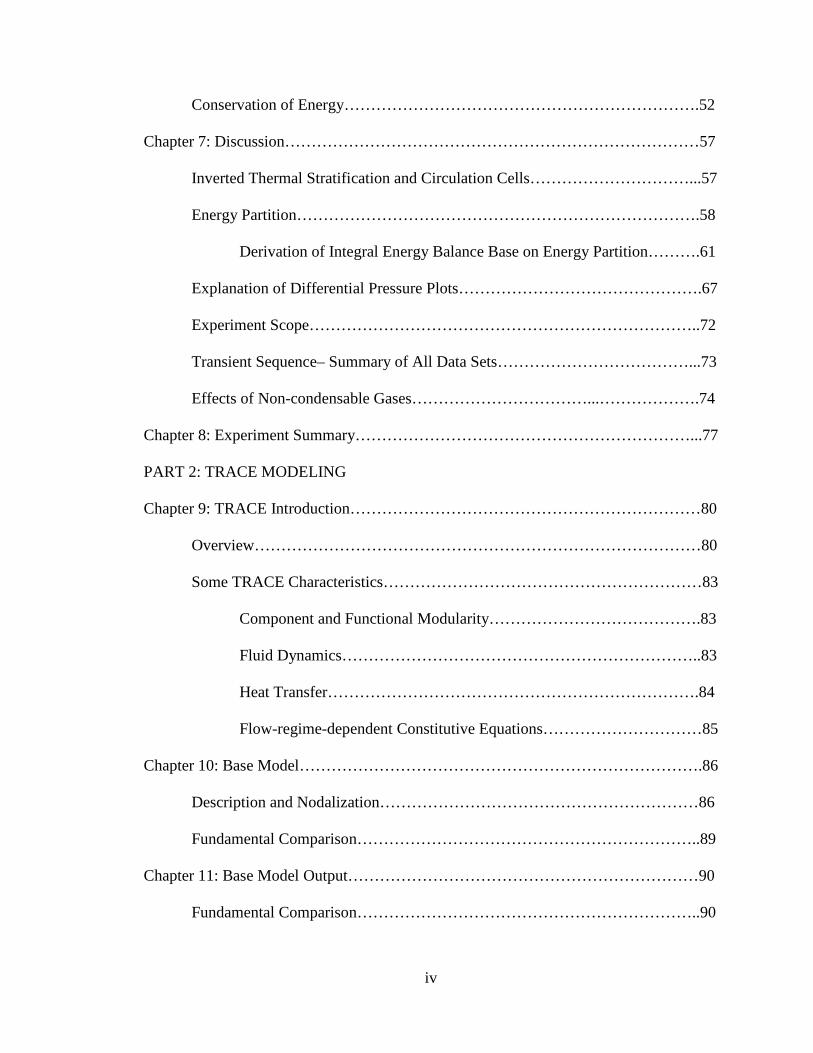
Conservation of Energy………………………………………………………….52 Chapter 7: Discussion……………………………………………………………………57 Inverted Thermal Stratification and Circulation Cells…………………………...57 Energy Partition………………………………………………………………….58 Derivation of Integral Energy Balance Base on Energy Partition……….61 Explanation of Differential Pressure Plots……………………………………….67
Experiment Scope………………………………………………………………..72 Transient Sequence– Summary of All Data Sets………………………………...73 Effects of Non-condensable Gases……………………………...……………….74
Chapter 8: Experiment Summary………………………………………………………...77 PART 2: TRACE MODELING Chapter 9: TRACE Introduction…………………………………………………………80 Overview…………………………………………………………………………80 Some TRACE Characteristics……………………………………………………83 Component and Functional Modularity………………………………….83 Fluid Dynamics…………………………………………………………..83 Heat Transfer…………………………………………………………….84 Flow-regime-dependent Constitutive Equations…………………………85 Chapter 10: Base Model………………………………………………………………….86 Description and Nodalization……………………………………………………86 Fundamental Comparison………………………………………………………..89 Chapter 11: Base Model Output…………………………………………………………90 Fundamental Comparison………………………………………………………..90

v
Other One-to-one Comparisons………………………………………………….92 Pressure…………………………………………………………………..92 Temperature……………………………………………………………...93 Inventory…………………………………………………………………97 Summary of Relevant Base Model Discrepancies……………………………….98 Chapter 12: Modifications to Base Model……………………………………………….99 List of Physical Phenomena Present in the Condenser Pipe……………………100 Mapping Phenomena to TRACE Parameters…………………………………..101 Base Model Modification Results and General Observations………………….103 Non-condensable Gas Modifications to Base Model…………………...106 VESSEL Modifications to Base Model………………………………...109 Chapter 13: Final TRACE Model………………………………………………………113 Nodalization Scheme…………………………………………………………...114 Fundamental Comparison………………………………………………………116 Other One-to-one Comparisons………………………………………………...118 Pressure…………………………………………………………………118 Temperature…………………………………………………………….120 Inventory………………………………………………………………..122 Chapter 14: Analysis of Main Discrepancies and Anomalies………………………….124 Over-stated Condensation Model………………………………………………125 Difference between Data and Model…………………………………...125 Implications……………………………………………………………..126 Possible Source of Discrepancy…………………………………...……126

vi
Possible Solution………………………………………………………..128 Chapter 15: Modeling Summary………………………………………………………..130 Chapter 16: Conclusions and Recommendations………………………………………132 Conclusions……………………………………………………………………..132 Recommendations and Future Work…………………………………………...135 Appendix A: Experimental Procedures Checklist…………………………………………138 B: Clausius-Clapeyron Primer………………………………………………….141 C: Integral Energy Balance Assumptions………………………………………143 D: Obtaining Energy Balance Parameters from Data……………………….….145 E: TRACE Terminology………………………………………………………..148 F: Conservation Equations in Finite Difference Form…………………………150 G: TRACE Input Decks………………………………………………………...153 H: Summary of Plot Parameters………………………………………………..192 References………………………………………………………………………………194

vii
LIST OF TABLES Table 1: Initial experimental conditions…………………………………………..14 Table 2: Local verification of nozzle manufacturer’s advertised K-factors………30 Table 3: Summary of experimental error and estimated uncertainty……………...30 Table 4: Summary of experiments performed…………………………………….31 Table 5: Table of masses used to perform energy balance………………………..54 Table 6: Energy balance spreadsheet for the EZNF0800 transient………………..54 Table 7: Energy balance spreadsheet for the EZNF0815 transient………………..54 Table 8: Energy balance spreadsheet for the EZNF1500 transient………………..55 Table 9: Energy balance spreadsheet for the EZNF1515 transient………………..55 Table 10: Energy balance spreadsheet for the EZNF3000 transient………………..56 Table 11: List of mechanisms found in the condenser pipe of MANOTEA……...100 Table 12: TRACE modifications………………………………………………….102 Table 13: List of modifications to the Base Model………………………………..104

viii
LIST OF FIGURES Figure 1: Schematic drawing of the University of Maryland – United
States Naval Academy Near One-dimensional Transient Experimental Apparatus………………………………………………….11
Figure 2: Schematic drawing illustrating selected preparation steps and
transient progression from initial conditions to termination……………..16 Figure 3: Parameter tree showing operating domains……………………………...20 Figure 4: Schematic of liquid inventory measuring apparatus (floats)…………….24 Figure 5: Comparison of liquid inventory obtained with the differential
pressure cell to that obtained with the floats for an EZNF3000 transient…………………………………………………………………..24
Figure 6: Time to drain MANOTEA pipe for known inventories………………….25 Figure 7: Raw temperature data as a function of time for the CC01 thermo-
couple during preparation and execution of a typical transient………….27 Figure 8: Two-point linear calibration curve for raw CC01 thermocouple data…...28 Figure 9: Calibrated temperature data for the CC01 thermocouple over
the duration of a typical transient………………………………………...28 Figure 10: Pressure vs. time after transient initiation for the EZNF0800 nozzle……33 Figure 11: Condenser centerline temperatures vs. time after transient
initiation for the EZNF0800 nozzle……………………………………...33 Figure 12: Condenser surface temperatures vs. time after transient
initiation for the EZNF0800 nozzle……………………………………...34 Figure 13: Boiler centerline and surface temperatures vs. time after
transient initiation for the EZNF0800 nozzle……………………………34 Figure 14: Differential pressure vs. time after transient initiation for
the EZNF0800 nozzle……………………………………………………35

ix
Figure 15: Pressure vs. time after transient initiation for the EZNF0815 nozzle……36 Figure 16: Condenser centerline temperatures vs. time after transient
initiation for the EZNF0815 nozzle……………………………………...36 Figure 17: Condenser surface temperatures vs. time after transient
initiation for the EZNF0815 nozzle……………………………………...37 Figure 18: Boiler centerline and surface temperatures vs. time after
transient initiation for the EZNF0815 nozzle……………………………37 Figure 19: Differential pressure vs. time after transient initiation for
the EZNF0815 nozzle……………………………………………………38 Figure 20: Pressure vs. time after transient initiation for the EZNF1500 nozzle……39 Figure 21: Condenser centerline temperatures vs. time after transient
initiation for the EZNF1500 nozzle……………………………………...39 Figure 22: Condenser surface temperatures vs. time after transient
initiation for the EZNF1500 nozzle……………………………………...40 Figure 23: Boiler centerline and surface temperatures vs. time after
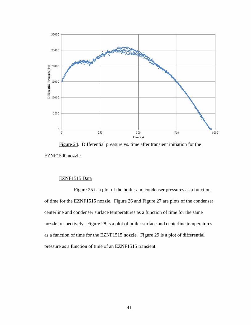
transient initiation for the EZNF1500 nozzle……………………………40 Figure 24: Differential pressure vs. time after transient initiation for
the EZNF1500 nozzle……………………………………………………41 Figure 25: Pressure vs. time after transient initiation for the EZNF1515 nozzle……42 Figure 26: Condenser centerline temperatures vs. time after transient
initiation for the EZNF1515 nozzle……………………………………...42 Figure 27: Condenser surface temperatures vs. time after transient
initiation for the EZNF1515 nozzle……………………………………...43 Figure 28: Boiler centerline and surface temperatures vs. time after
transient initiation for the EZNF1515 nozzle……………………………43 Figure 29: Differential pressure vs. time after transient initiation for
the EZNF1515 nozzle……………………………………………………44 Figure 30: Pressure vs. time after transient initiation for the EZNF3000 nozzle……45 Figure 31: Condenser centerline temperatures vs. time after transient
initiation for the EZNF3000 nozzle……………………………………...45

x
Figure 32: Condenser surface temperatures vs. time after transient initiation for the EZNF3000 nozzle……………………………………...46
Figure 33: Boiler centerline and surface temperatures vs. time after
transient initiation for the EZNF3000 nozzle……………………………46 Figure 34: Differential pressure vs. time after transient initiation for
the EZNF3000 nozzle……………………………………………………47 Figure 35: Liquid inventory vs. time after transient initiation for the
EZNF0800 nozzle………………………………………………………..49 Figure 36: Liquid inventory vs. time after transient initiation for the
EZNF0815 nozzle………………………………………………………..50 Figure 37: Liquid inventory vs. time after transient initiation for the
EZNF1500 nozzle………………………………………………………..50 Figure 38: Liquid inventory vs. time after transient initiation for the
EZNF1515 nozzle………………………………………………………..51 Figure 39: Liquid inventory vs. time after transient initiation for the
EZNF3000 nozzle………………………………………………………..51 Figure 40: Energy transferred from the wall versus volume transferred
from the boiler to the condenser pipe……………………………………60 Figure 41: Schematic drawing showing the control volume used to
derive integral energy balance based on the energy partition……………62 Figure 42: Implementation of Equation 3 with EZNF1500 experimental data……...66 Figure 43: Reproduction of Figures 10 (pressure vs. time) and 14 (differential
pressure vs. time), respectively…………………………………………..68 Figure 44: Boiler saturation analysis………………………………………………...70 Figure 45: Volume difference between 0 and 15-deg nozzle of fixed
cross-sectional area………………………………………………………73 Figure 46: Pressure as a function of condenser inventory for all nozzles…………...74 Figure 47: Nodalization and heat structure scheme for the Base TRACE
Model of MANOTEA……………………………………………………88

xi
Figure 48: Base Model output for condenser pressure as a function of
condenser inventory……………………………………………………...91 Figure 49: Base Model output for pressure versus time after transient initiation…...93 Figure 50: Base Model output for condenser centerline temperature
versus time after transient initiation……………………………………...95 Figure 51: Base Model output for condenser surface temperature
versus time after transient initiation……………………………………...95 Figure 52: Base Model output for boiler centerline temperature versus
time after transient initiation……………………………………………..96 Figure 53: Base Model output for mass (inventory) versus time after
transient initiation………………………………………………………..97 Figure 54: Parametric non-condensable gas study performed with TRACE………108 Figure 55: Top view of VESSEL component with 2 radial ring nodes
and 1 azimuthal node…………………………………………………...111 Figure 56: Nodalization and heat structure scheme for the Final TRACE
Model of MANOTEA………………………………………………….115 Figure 57: Fundamental comparison between MANOTEA data and
TRACE models…………………………………………………………116 Figure 58: Base and Final Model output for pressure versus time after
Transient initiation……………………………………………………...119 Figure 59: Base and Final Model output for condenser centerline temperature
versus time after transient initiation to transient termination…………..121 Figure 60: Base and Final Model output for inventory versus time after
transient initiation to transient termination……………………………..123

xii
LIST OF SYMBOLS Symbols Abbreviations Bi Biot number 1D 1 dimensional c specific heat 3D 3 dimensional D diameter BC boiler centerline E energy BS boiler surface f participating fraction BWR boiling water reactor H enthalpy CC condenser centerline h specific enthalpy CCDPHE counter-current, double-pipe K, k nozzle proportionality constant heat exchanger L, l length CS condenser surface m mass DP differential pressure P, p pressure, ratio of pressures DPHE double-pipe heat exchanger q heat transfer per unit mass EZNFXXYY EZNF: Bete nozzle R gas constant designator, XX: diameter, Ra Rayleigh number YY: spray characteristic T temperature ID inner diameter t time LOCA loss of coolant accident U internal energy MANOTEA UMD-USNA Near One- dimensional Transient Subscripts Experimental Assembly NRC Nuclear Regulatory D diameter Commission f final PWR Pressurized Water Reactor g gas RELAP Reactor Excursion and Leak i, o initial Analysis Program L, l liquid SETS Stability Enhancing Two-step m metal Techniques P pipe SNAP Symbolic Nuclear Analysis sat saturated Program sp spray TRAC Transient Reactor Analysis v vapor Code TRACE TRAC-RELAP Advanced Greek Computational Engine
TRAC-B TRAC-BWR ∆ change (final - initial value) TRAC-P TRAC-PWR Λ hf - hg UMD University of Maryland χ proportionality constant USNA U. S. Naval Academy WYSIWYG what you see is what you get

1
Chapter 1: Introduction Significance of Present Study
The purpose of the present work was to experimentally validate the
TRAC(Transient Reactor Analysis Code)/RELAP (Reactor Leak Analysis Program)
Advanced Computational Engine (TRACE) plug-in for the NRC’s Symbolic Nuclear
Analysis Package (SNAP) for a rapid condensation transient on a simplified, integral
apparatus with behaviour similar to those found in reactor systems. SNAP is the
“flagship” code of the U.S. Nuclear Regulatory Commission (NRC) and the sole tool
used to perform analysis and to certify new reactor designs (NRC, 2011b). The
TRACE plug-in is designed to analyze thermal-hydraulic system transients in light
water reactors (NRC, 2011b). The challenges that integral, condensation-driven
transients have posed to thermal-hydraulic codes provided the motivation for the
present work. The present work is particularly relevant because many of the
proposed passive safety systems found in next generation reactors rely on rapid
condensation for operation or accident mitigation. Although clearly a “beyond design
basis accident”, the recent sequence of events at the Fukushima Power Plant in Japan
highlights the continued relevance of reactor safety research efforts and accident
mitigation in general.
Approach and Objectives
The present work was undertaken in two phases: an experimental and
modeling phase. Data from the experimental phase was compared to output from a

2
TRACE model. Discrepancies between the data and the code output were used to
identify potential problem areas in the code. Recommendations for potential ways to
improve the code were then made based on this analysis.
In order to implement this approach, the following objectives were identified:
- Construct, instrument and calibrate an integral, condensation-driven transient
apparatus.
- Run a series of scoped experiments on the apparatus in order to identify
transient mechanisms and build a database.
- Develop a TRACE model of the transient apparatus.
- Make recommendations for code improvement by comparing experimental
data to TRACE output.
Dissertation Organization
This dissertation is organized into two main parts. Prior to the first part,
Chapter 2 is a literature review and introduces relevant topics. The first part
encompasses Chapters 3-8 and presents the details of the experimental portion of the
present work. The second part outlines efforts to model the experiment with TRACE
and encompasses Chapters 9-14. The final chapter draws conclusions from the
experimental and modeling portions, and makes recommendations based on these
conclusions.

3
Chapter 2: Literature Review Integral Transients
Over the years, the study of nuclear power plant accidents has evolved and
matured from hypothetical scenarios, which were defined by imposed assumptions, to
accident development sequences which maintain a physically coherent sequence of
events. Some of these sequences were later characterized as the “design basis
accidents.” Abramson (1985) generalized the information available about Small
Break- Loss of Coolant Accidents (SB-LOCAs) by suggesting a sequence of physical
events, complete with descriptions, which can be expected for transients during which
primary inventory is gradually lost. In a similar manner, Duffey and Sursock (1987)
traced the progression of an SB-LOCA in terms of system flow characteristics. As
part of the U.S. NRC’s Integral Systems Test (Young and Sursock, 1987), Di Marzo
and co-workers (1988) showed that a portion of an SB-LOCA is controlled by rapid
condensation occurring near saturation conditions. The definition of rapid
condensation usually includes the requirement that the induced fluid motion be
limited by fluid inertia rather than by the heat transfer rate (Block, 1980). These
works highlight the integral nature of an SB-LOCA, meaning the current state is the
cumulative result of all the previous states encountered in sequence. Furthermore, the
fundamental parameter characterizing each state is how much inventory has left the
system.
4
Rapid Condensation
Rapid condensation induced fluid motion is not limited to SB-LOCAs, but
occurs in numerous other accidents sequences and operating situations. Block
(1987), Bankoff (1980), and Kirchner and Bankoff (1985) each wrote overview
papers summarizing condensation induced fluid motion relevant to nuclear reactors.
As outlined in these papers, typical examples include: water slug delivery in an
annular downcomer, steam discharge into large pools of subcooled water like those
found in a suppression tank, cold leg oscillations induced by an Emergency Core
Cooling (ECC) injection, “reflux” condensation oscillations in U-tube steam
generators, and the condensation induced oscillations due to combined injection of
ECC liquid into both the hot and cold legs. These transient event sequences are
complicated to analyze because they involve 2-phase flow and 3-dimensional
geometry coupled with the integral effects. Historically, these multi-phase, multi-
dimensional, integral transients have proven challenging for thermal-hydraulic
computer codes such as those used for design certification (Wang, 1992).
Rapid Condensation in Generation III+ Reactors The U.S. Department of Energy (DOE) classifies the evolution of
nuclear reactor designs in terms of “generations” (Nuclear, 2002). Generation I
reactors were the early prototypes (Shippingport, Dresden, Fermi I, and Magnox).
Developed during the 1950s and 60s, these reactors were typically smaller-scale,
proof-of-concept, research reactors. Lessons learned from these reactors paved the
way for the development of large-scale, commercial, power generation reactors in the
1970s. These reactors are classified as Generation II and comprise all 104

5
commercial reactors currently operating in the United States (Nuclear Energy
Institute, 2011). Generation III reactors were developed in the 1990s. Primarily
built in East Asia, this generation of reactors modified Generation II designs to
improve safety and efficiency (Nuclear, 2002). Generation III+ reactors are those
currently under development and expected to be built in the near-term. This
generation includes the Advanced Passive 1000 Reactor (AP1000) and Economic
Simplified Boiling Water Reactor (ESBWR). Some details of these particular
reactors are outlined below. Generation IV reactors are those that the Department of
Energy would like to develop in partnership with 9 other countries coming together as
the Generation IV International Forum (GIF). The goal of the GIF is to develop
proliferation resistant, highly economical reactors with enhanced, passive safety
features and minimal waste. Such reactors are not intended to meet the immediate
need for power production, but rather to serve as the next generation (Nuclear, 2002).
The Westinghouse AP1000 and General Electric ESBWR are two generation III+
reactors that incorporate rapid condensation passive safety features.
Westinghouse AP1000 The Westinghouse Advanced Passive 1000 (AP1000) is a pressurized
water reactor designed to generate 1000 MWelectric from 3415 MWthermal. It contains
many features not found in current operating reactors. The most significant
improvement is use of safety systems that employ passive means such as gravity,
natural circulation, condensation and evaporation heat transfer, and stored energy for
accident mitigation. These passive systems perform safety injection, residual heat
removal, and containment cooling functions (Schulz, 2006).

6
Based on analysis of the design with SNAP, the NRC issued a final
design certification for the AP1000 in January of 2006. To date, 14 combined
operating licenses applications have been received by the NRC for construction of
AP1000 units in the U.S. Numerous reactors have also been ordered for construction
in China (NRC, 2011b).
General Electric ESBWR
The General Electric-Hitachi Economic Simplified Boiling Water
Reactor (ESBWR) is designed to operate at 4500 MWthermal. The design builds on
experience gained from the company’s Advanced Boiling Water Reactor (ABWR)
which was issued a final design certification by the NRC in 1997 (NRC, 2011b). The
new design contains many features not found in current operating reactors to include
the use of natural circulation for normal operations. The ESBWR also uses passive
means for accident mitigation (Beard, 2006).
General Electric-Hitachi submitted an application for standard design
certification to the NRC in 2005. The NRC is currently reviewing and analyzing the
design. In anticipation of design approval, 3 combined operating license applications
have already been received by the NRC. Overseas interest in this design is expected
to be great (NRC, 2011b).
Integral Experiments and Code Development
In the wake of Three Mile Island, reactor safety research took on a new sense
of urgency. The Nuclear Regulatory Commission (NRC) began placing greater
emphasis on operator training and human factors, emergency planning, plant
operating histories, and severe, non-design basis accidents resulting from small

7
equipment failures. Due to the nature of the Three Mile Island Accident, major effort
was dedicated to investigation of SB-LOCAs in particular (NRC, 2011b). This
renewed interest provided the motivation for a period of concentrated reactor safety
research, which is still relevant today.
The NRC has funded multiple experiments to classify and quantify steady
state and transient behavior in reactor systems. Data from facilities like Semiscale
(Loomis, 1987), Flecht-Seaset (Hochreiter, 1985), PKL (Hass, 1982), LOFT
(Nalezny, 1985), MIST (Geissler, 1987), and the UMCP Thermal-hydraulic Loop
(Hsu, 1987) were used to develop, modify, and validate thermal-hydraulic reactor
safety codes. These codes included, but were not limited to, the Reactor Excursion
and Leak Analysis Program (RELAP) and Transient Reactor Analysis Code (TRAC),
both of which focused on thermal-hydraulic analysis.
Since their inception, improvement and development of these analysis codes
has been continuous. The NRC distributes the latest versions of its codes as the
Symbolic Nuclear Analysis Package (SNAP). The package consists of an integrated,
interoperable series of “plug-in” applications that are designed to simplify
engineering analysis of reactor systems. These plug-ins were developed from legacy
codes such as RELAP and TRAC (which were merged into a single thermal-hydraulic
code and renamed TRAC-RELAP Advanced Computational Engine or TRACE).
Other legacy codes such as the Purdue Advanced Reactor Core Simulator (PARCS)
and Systems Analysis Programs for Hands-on Integrated Reliability (SAPHIRE) were
also included in the package. Through the use of these plug-ins, SNAP is able to

8
analyze and synthesize all aspects of reactor operations. The package is the sole
analysis tool used in modeling the behavior of new reactor designs (NRC, 2011b).
Since design certification is performed solely by computer code, it is of the
upmost importance that the code be able to accurately predict steady state and
transient behaviors in reactor systems. Inability of the codes to properly model
reactor behavior has serious implications and hinders our ability to properly train
operators, regulate, and address safety concerns. To ensure the analysis tools are of
the highest quality and can be used with the strictest confidence, the NRC encourages
users to challenge the code by comparing its predictions to data from a wide range of
applications to include novel designs and non-nuclear apparatus (NRC, 2011a).
Regular challenges and identification of areas for improvement ensure the code is
adequate to perform the certification mission. The present work is meant to challenge
the code for condensation transients. This work is useful because many new features
found in Generation III+ reactors rely on condensation.
Reactor behavior is extremely complex. To capture elements of this behavior,
a simplified apparatus has been constructed. The design of this apparatus is outlined
in Chapter 3. Due to its simplicity, the apparatus is easier to model with TRACE, but
still has behaviors similar to those of the more complex reactor system. If TRACE
can properly predict the behavior of the simplier facility, it lends confidence to the
code’s abilities to properly predict reactor behavior.

9
PART 1: EXPERIMENT

10
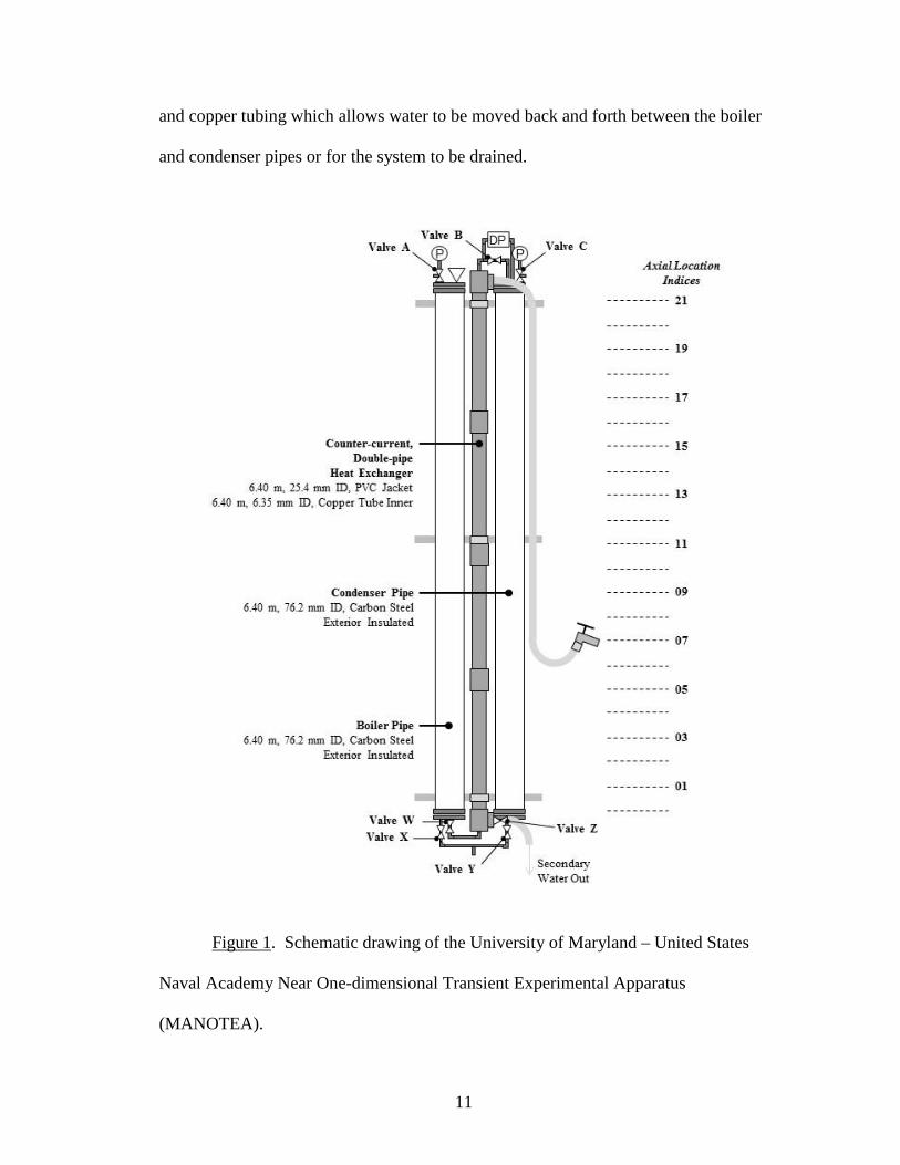
Chapter 3: Facility Description Apparatus Figure 1 is a schematic drawing of the University of Maryland-United States
Naval Academy Near One-dimensional Transient Experimental Apparatus
(MANOTEA). MANOTEA was constructed at the United States Naval Academy
during the summer of 2010. The facility consists of a boiler pipe, counter-current
double-pipe heat exchanger, condenser pipe, and appropriate data acquisition and data
logging systems (not shown in Figure 1).
The boiler pipe (6.40 m tall, 76.2 mm ID, 82.6 mm OD) is constructed from 2
commercially available, 3.05 m, schedule 40, carbon steel pipes held together by a
threaded coupling and capped at the ends with threaded flanges. Blanks were
machined for instrumentation and other fittings. These blanks were then bolted to the
top or bottom flanges, respectively. High temperature O-rings ensure a proper seal.
The exterior of the pipe is insulated with 50.8-mm-thick, fiberglass pipe insulation. A
1.00 kW ohmic heater is mounted in the bottom flange. The boiler pipe contains 3
centerline and 3 exterior surface thermocouples located at 0.30 m, 3.35 m, and 6.10 m
(nominally: 1’, 11’, and 21’ or axial locations 1, 11, and 21 on Figure 1) from the
bottom flange, respectively. A pressure transducer is mounted to a T-valve (Valve A)
in the top flange. The three-way valve allows the boiler to be vented to the
atmosphere or connected to the transducer. The top flange also contains an opening
for filling the apparatus with water. The bottom flange contains a valve (Valve X)
11
and copper tubing which allows water to be moved back and forth between the boiler
and condenser pipes or for the system to be drained.
Figure 1. Schematic drawing of the University of Maryland – United States
Naval Academy Near One-dimensional Transient Experimental Apparatus
(MANOTEA).

12
The counter-current double-pipe heat exchanger (DPHE) is constructed of
PVC (25.4 mm, schedule 80) and copper tubing (6.35 mm ID). Tap water enters the
secondary side through the top of the PVC outer pipe and exits through the bottom
into a drain. Warm water from the boiler enters the primary side through the bottom
via copper tubing and exits at the top through a solenoid valve (Valve B) on its way
to a nozzle in the vapor space of the condenser pipe. A thermocouple measures the
temperature of the primary fluid as it exits the DPHE. The heat exchanger is
sufficiently long with a secondary flow rate that ensures the primary fluid exits as
highly sub-cooled liquid (~20oC). A differential pressure cell (annotated as “DP” on
Figure 1) with one tap in the copper tubing as it exits the DPHE and one tap in the
vapor space of the condenser provides a means for measuring primary inventory flow
rate at the nozzle.
The condenser pipe is nearly identical to the boiler pipe – except it contains 11
centerline and 11 exterior surface thermocouples and the fill hole is replaced by one
of the differential pressure cell taps. The first thermocouple pair is located at 0.30 m
from the bottom flange and each successive pair advances up the length of the pipe in
0.61 m increments (axial locations 1, 3, 5…17, 19, 21, respectively). Scoping
experiments revealed that MANOTEA transients are condensation-controlled and that
a denser distribution of thermocouples would be required in the condenser to
adequately capture the relevant phenomena. The condenser and boiler pipes have an
aspect ratio of 84.
MANOTEA is not scaled to an actual reactor system or a feasibility study for
a future design. Rather, it is designed to be a simplified, integral, rapid condensation

13
transient device. Such transients have been a challenge to reactor safety codes. Yet,
condensation controlled phenomena are found in current and proposed reactor safety
systems. Reactors systems are extremely complex. MANOTEA is simple enough
that human reasoning and simple models can still capture its behavior, yet it still has
behaviors and features that tie it to the more complex reactor systems, namely: it is
integral in nature (this will be discussed more in a later section). Its simplicity
implies that it will be easier to model with a code like TRACE. All coding
difficulties have been eliminated, and thereby the code should have no problem
predicting MANOTEA behavior. Facility design and operating parameters were
chosen with the code in mind and with the intent of maximizing condensation effects.
Due to the simplicity of the MANOTEA facility, this experimental effort may prove
useful as a benchmark for next generation code development as well.
Facility Operation
Experiment preparation begins by filling the boiler pipe completely. The tee
at the lowest point of the apparatus is capped, and Valves X and Y are opened to
allow water to flow from the boiler to the condenser pipe, which results in each pipe
being half full. Roughly 3.8 L of water is measured out and added to the total
inventory. This additional water is required to ensure that neither of the heaters
becomes uncovered during the experiment. Both heaters (one at the bottom of the
boiler and one at the bottom of the condenser pipe) are turned on and the inventory is
allowed to heat up and boil for a minimum of 3 hours with Valves A and C in the top
flanges vented to the atmosphere. This process strips out the non-condensable gases.
Non-condensable gases are undesirable because they hinder the condensation process
that will occur during the actual experiment. After 3 hours, three-way Valve C in the

14
top of the condenser pipe is aligned to connect the vapor space to the pressure
transducer and the heater in the bottom of the boiler is turned off. Pressure in the
condenser builds up and moves liquid inventory to the boiler. Once a small amount
of water leaks out of Valve A at the top of the boiler, three-way Valve A is aligned to
connect the boiler vapor space to the pressure transducer, the boiler heater is turned
on again, the condenser heater is turned off, the boiler and condenser are isolated
from each other by closing Valves X and Y in the lower flanges, Valve W is opened
to allow boiler inventory to flow into the primary side of the DPHE, and DPHE
secondary water is turned on. The condenser is allowed to cool, this cooling takes
place by natural circulation and heat loss from the exposed top and bottom flange,
until the pressure in the condenser is roughly 101 kPa. While the condenser cools,
the pressure in the boiler is allowed to increase to roughly 121 kPa. The pressure
difference ensures all flow losses in the DPHE primary pipe are overcome and that
the transient will initiate. The preparation phase ends when the initial conditions are
achieved (see Table 1).
Boiler Condenser Initial Pressure (kPa) 121 101 Bulk Temperature (oC ) 105 100 Initial Inventory (L) 29.2 3.8
Table 1. Initial experimental conditions.
The transient is initiated, and the actual experiment begins, by opening the
solenoid valve (Valve B) at the top of the DPHE that leads to the condenser. This
allows primary liquid inventory to flow out of the boiler via the copper tubing, up
through the DPHE, and into the condenser pipe through a nozzle at the end of the

15
copper tubing in the vapor space. Sub-cooled liquid inventory enters the condenser at
the temperature of the secondary water (~20.0 oC). The transient, movement of liquid
inventory from the boiler to condenser via the DPHE, is driven by a pressure
differential that results from rapid condensation as the cool water enters the condenser
pipe. Scoping experiments revealed that the boiler pipe always provides sufficient
liquid by flashing adequate steam in the vapor space, never hindering the transient.
The duration of the transient and amount of liquid inventory transferred varies
depending on the nozzle size and geometry. The transient (movement of liquid
inventory from boiler to condenser via the double-pipe heat exchanger) is started by
the small pressure differential, but sustained by rapid condensation. How much
condensation occurs is controlled by a competition between condensation in the vapor
space, evaporation at the wall and liquid interface, and stored energy in the walls of
the condenser.
Figure 2 is a pictorial representation of the progress from setup (only selected
setup steps are shown) to transient termination.
A detailed, step-by-step checklist of procedures to prepare the facility and run
a transient is given in the appendix.

16
Figure 2. Schematic drawing illustrating selected preparation steps and
transient progression from initial conditions to termination.
The experimental parameters can be inferred from the facility description,
operating procedures, and initial conditions – namely: pressure, temperature, liquid
inventory, and nozzle geometry. The following section discusses the rational behind
certain parameters, procedures, and the initial conditions.

17
Facility Parameters Discussion
Pressure Experimental setup begins at atmospheric pressure because it makes
de-gassing the water easier. Non-condensable gasses are undesirable because they
hinder heat transfer/suppress condensation. Thus, the boiler and condenser are open
to the atmosphere to allow the non-condensable gasses to escape after being liberated
from the water by boiling. However, in spite of efforts to rid the system of non-
condensable gases, a small quantifiable fraction remains in the DPHE. These gases
will be discussed in more detail later.
The transient begins with a differential pressure (boiler pressure -
condenser pressure) of 21.0 kPa. This value insures there is sufficient pressure to
overcome loss (in the copper tubing, valves, tees, and orifices) and initiate the
transient when the solenoid valve is opened. It should be noted that this differential
pressure only starts the transient, but rapid condensation sustains it. Higher pressure
implies more vapor which means diminished condensation for the same amount of
cooling spray entering the condenser. Choosing an initial pressure of 101 kPa in the
condenser means condensation effects will be maximized. With the condenser
pressure set at 101 kPa and the pressure differential set at 21.0 kPa, transient
initiation temperatures follow since the boiler and condenser are always at a
saturation condition.
Temperature As discussed above, initial condenser pressure is 101 kPa meaning
initial temperature is 100 oC on average. However, due to the setup process, there is a

18
temperature gradient with the bottom of the condenser being warmer due to its
proximity to the heater. This is possible because the liquid above presses on the
liquid below, making the saturation condition for lower liquid different from that of
the higher. These inverted thermal gradients are a direct consequence of the setup
process. A pressure differential of 21.0 kPa sets the boiler temperature at 105 oC on
average at transient initiation, but has a gradient for the reason just outlined. These
temperature gradients become important when performing an energy balance.
The secondary water comes from the tap at about 20.0 oC (varying
from 16-22.0 oC with season) and flow is sufficient to insure primary liquid enters the
nozzle in the condenser at 20.0 oC. Thus, flow exiting the boiler is at a saturation
condition and flow entering the condenser is single-phase. Highly sub-cooled liquid
was desired because it ensures single phase liquid enters the condenser via the nozzle.
Two-phase flow is much more complex and less understood. As a result, two-phase
flow has historically been more difficult for the code. Single-phase liquid provides a
simple means for measuring flow through the nozzle and should be easy for TRACE
to capture. Secondary water exits to a drain and final temperature is not measured or
desired.
Initial Liquid Inventory An initial condenser inventory of 3.8 L ensures that the heater stays
covered during experiment preparation. Beginning the transient with the boiler full
means less pressure head needs to be overcome in order for the liquid inventory to go
over the top of the DPHE as it enters the condenser pipe. This translates to lower

19
operating temperatures and increased condensation for a given amount of cool spray
entering the condenser.
Nozzle Geometry The shape and size (diameter) of the nozzle, which is the only thing
that was varied between experiments, dictates whether sub-cooled liquid entering the
condenser hits the pipe walls or falls predominantly into the vapor space. Sub-cooled
liquid flowing through a fan nozzle will hit the wall and collapse less vapor. Sub-
cooled liquid flowing through a jet nozzle will fall predominantly into the vapor
space, collapsing more vapor and doing more pressure-volume work. A small
diameter nozzle means less primary liquid enters during a given time interval. In this
case, the metal masses (stored energy) will dominate heat transfer and can actually
prevent the transient from beginning properly. For a mid-sized nozzle, sufficient
inventory can enter the condenser pipe and condensation rate will drive the transient.
If a large diameter nozzle is used, flashing rate in the boiler pipe could constrain and
control the transient. Although theoretically possible, an experiment - ran as part of
our scoping matrix - without a nozzle at all (open copper end) revealed that flashing
controlled transients are not possible on the MANOTEA. Thus, large-nozzle
MANOTEA transients are condensation controlled. Larger diameter nozzles allow
more cool liquid to enter during a given time, resulting in shorter transients. By
varying nozzle geometry and size, different transients can be obtained. Thus,
intuitively nozzle size and geometry will effect transient duration and amount of
liquid inventory.

20
A test matrix outlining the nozzle used during the current work is
outlined in Chapter 5. The results of the present work, outlined in a later Chapter 6,
confirm the analysis outlined in the preceding paragraph.
Operating Domains
From the operating parameters, and the discussion in the proceeding section, it
can be inferred that transient behavior can be classified into 3 operating domains.
Depending on whether the incoming inventory (spray) interacts with the pipe wall
and how much inventory enters (nozzle diameter), transients controlled by the metal
mass, condensation rate, flashing rate, or a combination of these are possible. These
operating domains are summarized with the parameter tree shown in Figure 3. Again,
flashing controlled MANOTEA transients are not possible. Overall transient
outcome can be viewed as a competition between these operating domains.
Figure 3. Parameter tree showing operating domains.
In Chapter 7, the concept of an energy partition is introduced. The energy
partition builds on the concept of operating domains to delineate how much of the

21
incoming (spray) enthalpy goes to collapsing vapor and how much goes to cooling
the pipe wall. The energy partition concept can then be used to derive a “back of the
envelope” integral energy balance equation.

22
Chapter 4: Instrumentation After MANOTEA was constructed, a series of scoping and shakedown
experiments were conducted. The shakedown experiments verified that the facility
was working properly and could produce repeatable and meaningful data. As part of
the scoping evolution, calibration procedures and techniques were established. This
chapter outlines how instrumentation in the MANOTEA facility was calibrated or
verified for accuracy. The results of the scoping experiments were used to generate
an experiment matrix that will be outlined in Chapter 5 and discussed in Chapter 7.
Differential Pressure Cell A differential pressure (DP) cell (annotated as “DP” on Figure 1) with one tap
in the sub-cooled liquid as it exits the DPHE and one tap in the vapor space of the
condenser provided a means for measuring primary inventory flow rate and closing
the mass balance. A commercially available Omega PX409-015WDUV differential
pressure transducer with 5 point factory calibration was used to obtain differential
pressure as a function of time. Error was estimated at +/- 0.5% of full scale on
average (never to exceed +/- 1.0% of full scale), or about +/- 500 Pa. How the mass
balance was closed with a DP reading will be outlined in detail in Chapter 7. The
mass balance was verified against results obtained with the DP cell by using a novel
buoyant rod apparatus. These results were then double-checked with the aid of drain

23
curves. Final inventory values obtained with the 3 methods differed by about 0.50 L
on average, and rarely more than 1.0 L.
Buoyant Rod Apparatus
Figure 4 is a schematic drawing of the apparatus which will be referred to as
“floats” or “the floats”. A high-temperature plastic rod runs the entire length of the
boiler and condenser pipes (one apparatus is in each pipe) and penetrates the lower
and upper blanks. The lower end of the rod feeds into a cylindrical port that allows
the rod to slide up and down while preventing liquid inventory from leaking out. The
upper penetration is shown in detail in the figure. Standard cast iron pipe fittings
maintain the system boundary. The high-temperature plastic rod is connected to the
free end of a tempered-steel beam. The fixed end of the beam is secured in a 1/2”
pipe-size NPT cap. Two strain gauges are placed at the root of the bending beam, one
on the top and one on the bottom. In this configuration, the strain reading is
temperature independent. Strain readings for known inventories, such as with the
pipes full and empty, provide boundary conditions or calibration points. With this
information liquid level in the pipe (which causes the beam to deflect up or down)
can be correlated to a strain reading. Keeping track of strain readings with respect to
time provides an alternate means of obtaining liquid inventory in the boiler and
condenser. Figure 5 is a graph comparing the liquid inventory obtained with the
differential pressure cell to that obtained with the floats. The floats give confidence
to the flow rate and subsequent liquid inventory data obtained with the DP cell.

24
Figure 4. Schematic of liquid inventory measuring apparatus (floats).
Figure 5. Comparison of liquid inventory obtained with the differential
pressure cell to that obtained with the floats for an EZNF3000 transient.

25
Drain Curves
A second method to reverify the mass balance was performed with the
aid of drain curves. The boiler and condenser pipes were each filled to known
volumes. The time to drain each pipe (separately - with the vent valve at the top of
each pipe open to the atmosphere) was subsequently monitored. Figure 6 is a plot of
this data with a least squares fit line applied. At the end of each experiment, the
boiler and condenser pipes were drained separately and the time to drain recorded.
Adjusting drain times for temperature (viscosity) yielded a good final inventory check
and also served to reinforce the validity of the mass balance obtained with the
differential pressure cell.
Figure 6. Time to drain MANOTEA pipe for known inventories at room
temperature.

26
Thermocouples Thirty type-J thermocouples connected to three Pico Technology TC-08 data
loggers were used to track temperature as a function of time. Temperature data was
then used to close the energy balance. By National Institute of Standards and
Technology (NIST) standards, error for “standard” type-J thermocouples should be
less than +/- 2.2 oC. Each TC-08 data logger came with a 12-point calibration for the
temperatures ranging from -100 to 1200 oC. Based on the calibration, for the range of
temperatures found in MANOTEA, an additional error of no more than +/- 0.50 oC
can be attributed to the data logger.
Data loggers are extremely sensitive to humidity. Since MANOTEA was
built in a laboratory without temperature control near the Severn River, humidity was
a concern and ensuring the integrity of the data paramount. Prior to each experiment,
the temperature of the lab was compared to the cold junction reading on the three data
loggers. After the experiment raw data was downloaded from the loggers and plotted.
Knowing the initial temperature was the temperature of the lab and knowing that
temperature would level at 100 oC during the boiling/stripping process, a two point
calibration was possible. These two points were plotted and a linear fit was
performed with a spreadsheet program in order to obtain a mapping or calibration
equation. The raw data from each thermocouple was individually mapped and
‘temperature versus time plots’ were generated for the respective transient. Figure 7
is a plot of the typical raw temperature as a function of time data for “CC01”. The
figure shows temperature readings from the moment the boiler was filled through the
termination of the experiment, to include all preparation steps. Steps are labeled on

27
the figure. Figure 8 is a plot showing the calibration curve for the same thermocouple
during the same transient. Figure 9 is a plot of the calibrated temperature versus time
after transient initiation for the data shown in Figure 7 and the calibration curve
shown in Figure 8. Note, due to variations in humidity, this calibration process was
performed for every thermocouple and every experiment.
Figure 7. Raw temperature data as a function of time for the CC01
thermocouple during preparation and execution of a typical transient.

28
Figure 8. Two-point linear calibration curve for raw CC01 thermocouple data
shown in Figure 7.
Figure 9. Calibrated temperature data for the CC01 thermocouple over the
duration of a typical transient.

29
Pressure Transducers The boiler and condenser pipe both have a MicroDAQ LOGiT pressure
transducer mounted in their top flange, respectively. The transducers came with a 5-
point NIST calibration certificate. Since each transient occurred under saturation
conditions, these pressure readings provided a convenient, independent means to
verify the bulk temperature profiles in the boiler and condenser. In addition, these
devices provide an independent verification of the DP cell readings. Data from these
pressure transducers were used to generate pressure as a function of time and pressure
as a function of inventory plots. This specific transducer was chosen because the
accompanying data logging system was sufficiently robust and easy to install and use.
The pressure transducers were “zeroed” before every experiment. Error from the
transducer and logging systems was estimated to be no more than 1% of full scale or
about +/- 10000 Pa.
Nozzles In order to ensure the accuracy of the mass balance, it was necessary to verify
the K-factors (nozzle loss coefficients) advertised for the EZNF series nozzles used in
MANOTEA. How the mass balance was closed using a DP cell reading and K-factor
will be outlined in detail in Chapter 6.
K-factor verification was performed locally by attaching a “T”, with an EZNF
nozzle on one opening and a pressure gauge on the other, to the end of a hose. Water
exiting the nozzle was directed into a graduated cylinder, and time to transfer a
measured volume was tracked with a stop watch. The results of this effort for 3
nozzles are shown in Table 2. The local verification for the 3 nozzles revealed that

30
the manufacturer’s K-factors are acceptably accurate. Since the K-factors for these
nozzles were acceptable, verification of all the nozzles used was deemed unnecessary
and not performed. Local verification was somewhat crude, but the confidence
gained by performing it was invaluable. The largest source of error in the local
verification process was the pressure reading, which was taken with a simple analog
gauge with 1- psi marks. The local verification values were within 10% of the
advertised values.
Table 2. Local verification of nozzle manufacturer’s advertised K-factors.
Highlighted columns show advertised K-factor & minimum and maximum values
obtained by local test.
Summary of Estimated Error Table 3 summarizes the estimated error for each measured or calculated
parameter in MANOTEA.
Parameter Estimated Maximum Error/Uncertainty
Raw Temperature +/- 2.7 oC Differential Pressure Gauge +/- 500 Pa Boiler/Condenser Pressure Transducer +/- 10000 Pa Inventory/Inventory Transfer +/- 0.50 L
Table 3. Summary of experimental error and estimated measurement
uncertainty.

31
Chapter 5: Test Matrix and Experimental Data
Table 4 is an outline of the experiments performed as part of the present work.
All experiments were ran as described in Chapter 3. Each experiment was performed
at least twice in order to verify repeatability. Nozzle size and geometry was varied in
order to obtain transients of different duration and differing amounts of inventory
transfer. All nozzles were purchased from the BETE Spray Nozzle Company and are
commercially available. EZNF denotes the nozzle model. The next two digits denote
orifice diameter and the last two digits denote spray characteristics.
Initial Initial Initial Spray Equivalent Boiler Cond. Pressure Bete Nozzle ID Characteristic Orifice Dia K-factor Inv. Inv. Differential (mm) (L) (L) (kPa)
EZNF0800 0-deg (Jet) 1.83 1.82 29.2 3.8 21 EZNF0815 15-deg (Fan) 1.83 1.82 29.2 3.8 21 EZNF1500 0-deg (Jet) 2.38 3.42 29.2 3.8 21 EZNF1515 15-deg (Fan) 2.38 3.42 29.2 3.8 21 EZNF3000 0-deg (Jet) 3.57 6.84 29.2 3.8 21
Table 4. Summary of experiments performed.
Results by Nozzle Data from each of the experiments performed includes boiler pressure,
condenser pressure, temperatures (at those locations described in Chapter 3), and
differential pressure, all as a function of time. Differential pressure is used to
measure primary inventory flow rate and close the mass balance. Temperature data is

32
used in conjunction with the mass balance to close the energy balance. Mass and
energy balances will be presented in Chapter 6.
When plotting variables (pressure and temperature) with respect to time, each
of the data sets listed in Table 4 stands alone. Plotting pressure (and therefore bulk
temperature, because the systems is at saturation) with respect to the amount of liquid
inventory transferred is a useful way to compare datasets from all nozzle sizes and
geometries. When this is done for all the data sets and the results plotted on the same
axis, all the transients collapse and overlap. This feature will be discussed in more
detail in Chapter 7.
EZNF0800 Data
Figure 10 is a plot of the boiler and condenser pressures as a function
of time for the EZNF0800 nozzle. Figure 11 and Figure 12 are plots of the condenser
centerline (or fluid bulk) and condenser metal surface temperatures, at the 11
elevations outlined in Chapter 3, as a function of time for the same nozzle,
respectively. Figure 13 is a plot of boiler surface and centerline temperatures as a
function of time at the 3 lateral locations previously described. Legend labels in the
temperature plots are of the form CC01 (which would indicate Condenser Centerline
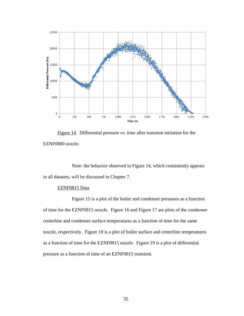
temperature at axial location 01 as annotated on Figure 1). Figure 14 is a plot of
differential pressure as a function of time of an EZNF0800 transient. Note:
throughout this dissertation, timescales were chosen based on transient duration.

33
Figure 10. Pressure vs. time after transient initiation for the EZNF0800
nozzle.
Figure 11. Condenser centerline temperatures vs. time after transient
initiation for the EZNF0800 nozzle.

34
Figure 12. Condenser surface temperatures vs. time after transient initiation
for the EZNF0800 nozzle.
Figure 13. Boiler centerline and surface temperatures vs. time after transient
initiation for the EZNF0800 nozzle.
35
Figure 14. Differential pressure vs. time after transient initiation for the
EZNF0800 nozzle.
Note: the behavior observed in Figure 14, which consistently appears
in all datasets, will be discussed in Chapter 7.
EZNF0815 Data
Figure 15 is a plot of the boiler and condenser pressures as a function
of time for the EZNF0815 nozzle. Figure 16 and Figure 17 are plots of the condenser
centerline and condenser surface temperatures as a function of time for the same
nozzle, respectively. Figure 18 is a plot of boiler surface and centerline temperatures
as a function of time for the EZNF0815 nozzle. Figure 19 is a plot of differential
pressure as a function of time of an EZNF0815 transient.

36
Figure 15. Pressure vs. time after transient initiation for the EZNF0815
nozzle.
Figure 16. Condenser centerline temperatures vs. time after transient
initiation for the EZNF0815 nozzle.

37
Figure 17. Condenser surface temperatures vs. time after transient initiation
for the EZNF0815 nozzle.
Figure 18. Boiler centerline and surface temperatures vs. time after transient
initiation for the EZNF0815 nozzle.

38
Figure 19. Differential pressure vs. time after transient initiation for the
EZNF0815 nozzle.
EZNF1500 Data
Figure 20 is a plot of the boiler and condenser pressures as a function
of time for the EZNF1500 nozzle. Figure 21 and Figure 22 are plots of the condenser
centerline and condenser surface temperatures as a function of time for the same
nozzle, respectively. Figure 23 is a plot of boiler surface and centerline temperatures
as a function of time for the EZNF1500 nozzle. Figure 24 is a plot of differential
pressure as a function of time of an EZNF1500 transient.

39
Figure 20. Pressure vs. time after transient initiation for the EZNF1500
nozzle.
Figure 21. Condenser centerline temperatures vs. time after transient
initiation for the EZNF1500 nozzle.

40
Figure 22. Condenser surface temperatures vs. time after transient initiation
for the EZNF1500 nozzle.
Figure 23. Boiler centerline and surface temperatures vs. time after transient
initiation for the EZNF1500 nozzle.
41
Figure 24. Differential pressure vs. time after transient initiation for the
EZNF1500 nozzle.
EZNF1515 Data
Figure 25 is a plot of the boiler and condenser pressures as a function
of time for the EZNF1515 nozzle. Figure 26 and Figure 27 are plots of the condenser
centerline and condenser surface temperatures as a function of time for the same
nozzle, respectively. Figure 28 is a plot of boiler surface and centerline temperatures
as a function of time for the EZNF1515 nozzle. Figure 29 is a plot of differential
pressure as a function of time of an EZNF1515 transient.

42
Figure 25. Pressure vs. time after transient initiation for the EZNF1515
nozzle.
Figure 26. Condenser centerline temperatures vs. time after transient
initiation for the EZNF1515 nozzle.

43
Figure 27. Condenser surface temperatures vs. time after transient initiation
for the EZNF1515 nozzle.
Figure 28. Boiler centerline and surface temperatures vs. time after transient
initiation for the EZNF1515 nozzle.

44
Figure 29. Differential pressure vs. time after transient initiation for the
EZNF1515 nozzle.
EZNF3000 Data
Figure 30 is a plot of the boiler and condenser pressures as a function
of time for the EZNF3000 nozzle. Figure 31 and Figure 32 are plots of the condenser
centerline and condenser surface temperatures as a function of time for the same
nozzle, respectively. Figure 33 is a plot of boiler surface and centerline temperatures
as a function of time for the EZNF3000 nozzle. Figure 34 is a plot of differential
pressure as a function of time of an EZNF3000 transient.

45
Figure 30. Pressure vs. time after transient initiation for the EZNF3000
nozzle.
Figure 31. Condenser centerline temperatures vs. time after transient
initiation for the EZNF3000 nozzle.

46
Figure 32. Condenser surface temperatures vs. time after transient initiation
for the EZNF3000 nozzle.
Figure 33. Boiler centerline and surface temperatures vs. time after transient
initiation for the EZNF3000 nozzle.

47
Figure 34. Differential pressure vs. time after transient initiation for the
EZNF3000 nozzle.

48
Chapter 6: Data Analysis Conservation of Mass A commercially available Omega PX409-015WDUV differential pressure cell
with one tap in the primary stream as it exits the DPHE and one tap in the vapor space
of the condenser was used to close the mass balance. The differential pressure gauge
was 5-point factory calibrated and local verification of this calibration was conducted
with a novel level measuring device based on buoyancy, as outlined in Chapter 4. In
addition to this verification, “drain curves” were generated by filling the boiler and
condenser pipes to known levels, monitoring the time for each pipe to drain, and then
curve fitting the data points. Initial boiler and condenser inventories were known,
and the drain curves served as a secondary means to verify the final inventories that
were obtained with the differential pressure gauge.
The differential cell measured pressure as a function of time. This data was
used to obtain liquid inventory flow rate from the boiler to the condenser pipe using
the equation:
Flow rate = K , (1)
where K is the nozzle proportionality constant or loss coefficient provided by the
manufacturer (and also verified locally) and ∆p is the pressure differential obtained
during the experiment and shown in Chapter 5. Using this equation, graphs of liquid
inventory vs. time were generated for each transient. Figures 35, 36, 37, 38, and 39
are plots of liquid inventory as a function of time for the EZNF0800, 0815, 1500,

49
1515, and 3000 transients, respectively. Note that nozzle geometry effects transient
duration and amount of liquid inventory transferred during the transient. These
differences arise due to differing energy transfer mechanisms and will be discussed in
more detail in Chapter 7.
Figure 35. Liquid inventory versus time after transient initiation for the
EZNF0800 nozzle.

50
Figure 36. Liquid inventory versus time after transient initiation for the
EZNF0815 nozzle.
Figure 37. Liquid inventory versus time after transient initiation for the
EZNF1500 nozzle.

51
Figure 38. Liquid inventory versus time after transient initiation for the
EZNF1515 nozzle.
Figure 39. Liquid inventory versus time after transient initiation for the
EZNF3000 nozzle.

52
Conservation of Energy
In order to enable calculation of an energy balance, the condenser pipe was
discretized into 12 nodes or cells. The nodes where assigned based on the location of
instrumentation, such as thermocouples. Again, scoping experiments revealed that
vapor generation in the boiler pipe is sufficient to continuously supply sub-cooled
liquid to the condenser. Thus, the boiler does not control the transient and an energy
balance for the boiler pipe is not necessary. The total mass (metal & liquid) in each
node on the condenser side was calculated. Using the temperature data and the mass
balance, initial and final internal energy was calculated for each cell. Heat losses
from the header and footer of the condenser pipe were estimated based on transient
duration and loss estimates made (during calibration experiments) by filling the
condenser, heating to a known temperature, and allowing the pipe to cool while
recording how temperature changed with respect to time. Knowing the volume and
temperature of the incoming sub-cooled liquid, spray enthalpy was calculated. The
energy balance was implemented with the aid of an Excel spreadsheet by plugging
these values into the equation 2:
Σ(Ui )cell + Hsp + Eloss = Σ(Uf)cell Σ(Uf - Ui )cell = Hsp + Eloss Σ[(cmmmTm + clmlTl)f - (cmmmTm + clmlTl)i ] cell = Vl h + Eloss (2) where Ui is the initial internal energy for each cell, Hsp is the enthalpy of the
incoming spray, Eloss is the estimated energy loss from the header/footer, Uf is the
final internal energy for each cell, cm is the specific heat of carbon steel (the pipe
walls), mm is the metal mass of each cell, Tm is the surface temperature (i.e.: CS01) of

53
each cell, cl is the specific heat of liquid (saturated water), ml is the mass of the
liquid in each cell, Tl is the temperature of the liquid in each cell (i.e.: CC01), Vl is the
total of volume of the liquid transferred during the transient, and h is the specific
enthalpy of the incoming spray (around 20 oC). Equation 2 is essentially a
differential energy balance based on the initial and final states. It has been mentioned
that MANOTEA transient are integral. Because only initial and final data was used,
Equation 2 does not capture the details of our integral transients, and is thereby an
approximation. A derivation of an integral energy balance in given in Chapter 7. The
integral energy balance is much more complicated to implement, and the complexity
does not buy a proportional amount of accuracy. The advantage of the integral
energy balance is that it gives insight into the physics behind the transient, whereas
Equation 2 is a quick, simple way to verify that the data satisfies conservation of
energy.
Table 5 shows the mass associated with each cell and defines cell
nomenclature. Tables 6-10 are the energy balance spreadsheets for the EZNF0800,
0815, 1500, 1515, and 3000 transients, respectively. The shaded boxes in Tables 6-
10 are the calculated values (in Joules) for the left and right-hand sides of Equation 2.
The calculated values differ by less than 5%, as annonated in the figure captions,
indicating that the data satisfies the conservation of energy law within reasonable
uncertainty limits.

54
Metal Mass (kg) Initial Liquid Mass (kg) Final Water Mass (kg) Header 8.99 1.33 1.38 Footer 5.05 Not applicable Not applicable “Standard” Cell 7.88 2.66 2.75 Table 5. Table of masses used to perform energy balance.
Table 6. Energy balance spreadsheet for the EZNF0800 transient. Shaded
boxes show calculated values for the left and right-hand side of Equation 4. Left and
right-hand sides are within ~4%.
Table 7. Energy balance spreadsheet for the EZNF0815 transient. Left and
right-hand sides are within ~5%.

55
Table 8. Energy balance spreadsheet for the EZNF1500 transient. Left and
right-hand sides are within ~2%.
Table 9. Energy balance spreadsheet for the EZNF1515 transient. Left and
right-hand sides are within ~5%.

56
Table 10. Energy balance spreadsheet for the EZNF3000 transient. Left and
right-hand sides are within ~3%.
57
Chapter 7: Discussion Inverted thermal stratification and circulation cells
Thermal stratification was observed in the condenser pipe for all experiments.
Furthermore, this stratification can be described as inverted, because cooler liquid is
resting on top of warmer liquid. Thermal inversion layers are common in
meteorology, oceanography (Steele, 2009), and, to a lesser extent, nuclear science
(Kloppers, 2005). In the MANOTEA experiment, inverted thermal stratification is
indicative of an interesting saturation condition in which cooler, denser liquid rests on
warmer, less dense liquid. This inverted stratification occurs primarily due to our
setup procedures. After venting non-condensable gases, the heater in the condensing
pipe is left on and pressure is allowed to build-up in order to fill the boiler pipe. This
heat-up phase establishes a temperature gradient over the length of the pipe, with the
bottom being much warmer than the top due to its proximity to the heater. Once the
transient is initiated and cool spray enters the condenser pipe from the top, the
temperature gradient is maintained by lack of fluid circulation. Calculations
performed with the aid of Locke (1992), reveal:
RaL1/4 = 4.86 [dimensionless force]
tD = 0.0662 [dimensionless time]
2L/D = 186 [dimensionless length]
If RaL1/4 << 2L/D and tD << 2, the fluid is said to be in the “impeded regime”.
Thus, MANOTEA transients occur in an impeded regime, meaning: convection is

58
occurring in small cells (on the order of the diameter of the pipe), at best, capable of
communicating only with its nearest neighbors, but vertical or bulk convection is
non-existent. Thus, over the relatively short time scale characterized by the duration
of a MANTOEA transient, heat transfer within the pooled liquid is occurring
primarily by conduction alone. This is a direct consequence of the facility’s large
aspect ratio. As cooling spray enters, the conduction mechanism cannot transfer
energy rapidly enough and little or no mixing occurs. The cooler upper layers end up
pressing on the warmer lower layers, providing enough pressure to compensate for
temperature-related density differences and maintain equilibrium. Thus, the entire
pipe is in equilibrium at a saturation condition with inverted thermal stratification.
Inverted thermal stratification was not anticipated, but is an interesting feature of the
MANOTEA facility.
Energy Partition
In general it can be said that the size or diameter of the nozzle effects transient
duration by allowing more cool spray to enter the condenser pipe during a given time.
Thus, for all other things constant, larger diameter nozzles result in faster transients.
Unfortunately, this does not give direct insight into how much liquid will be
transferred during a transient.
Nozzle geometry effects transient behavior by putting more or less sub-cooled
spray on the wall. Subcooled liquid flowing through a fan nozzle hits the pipe wall
and cools it, but collapses less vapor. Subcooled liquid flowing through a jet nozzle
will fall predominantly into the vapor space, collapsing more vapor and doing more
pressure-volume work but not cooling the wall to the same degree as a fan nozzle
59
with the same diameter. Thus, by doing more pressure-volume work jet nozzles
result in more inventory transfer. For a jet nozzle, more of the enthalpy of the
incoming subcooled spray goes into collapsing vapor than to cooling the pipe walls.
Figure 40 is a plot of energy transferred from the wall versus volume of liquid
transferred from the boiler to the condenser pipe during MANOTEA transients. The
figure illustrates how the energy partition, that is what amount of the available,
incoming, negative energy (enthalpy) goes into collapsing vapor and what amount
goes into cooling the pipe wall, effects inventory transfer. Although not part of the
experimental matrix, a transient was ran with an EXNF3015 nozzle in order to
determine inventory transferred. For large nozzles, the energy partition has little
effect because enough cool spray is entering the condenser to overwhelm the system
regardless of nozzle geometry (a rapid condensation transient). As nozzle size
decreases, the effects of the energy partition become apparent as an ever increasing
difference in the amount of liquid transferred. In the figure, the energy lost by the
wall was calculated from the energy balances and liters transferred were taken from
the mass balances, both outlined in Chapter 7. The heavy black line suggests the
location of a domain delimiter (in the sense described in Chapter 3), but is not based
on calculations.

60
Figure 40. Energy transferred from the wall versus volume transferred from
the boiler pipe to the condenser pipe. Plot shows effect of energy partition. Heavy
line suggests domain delimiter: somewhere between the two geometries, 15-deg
nozzles put more energy into pipe wall and 0-deg nozzles put more energy into vapor.
The energy partition is important for understanding the physics behind the
different transients and proves useful when interrogating the TRACE code. It
captures the operating domains outlined in Chapter 3. From the data, it can be
inferred that nozzle size is mainly responsible for transient duration and nozzle
geometry dictates how much inventory will be transferred. However, in reality,
duration and inventory transfer is a complex interplay between size and geometry that
can be captured only in terms of this energy partition. Yet, it is interesting to note
that each of the transients follows the exact same sequence regardless of nozzle size

61
or geometry. This statement will be justified in the one of the following discussion
sections. The importance of the energy partition is the insight it provides into the
physics controlling each transient. Although the energy partition is never quantified
in the present work because it is difficult to compare directly to TRACE, it is useful
and informative to derive an energy balance based on the energy partition.
Derivation of Integral Energy Balance Based on Energy Partition Principle Liquid mass leaving the boiler is always equal to the liquid mass
entering the condenser. Regardless of nozzle, every transient is controlled by a
competition between the energy in the metal masses and the energy in the incoming
spray. This competition in turn dictates the differential pressure. Coupling these
observations with our discovery that a flashing controlled transient is not possible on
the MANOTEA allows us to perform an energy balance by investigating the
condenser pipe alone. Figure 41 is a schematic of the control volume that will be
used to derive an energy balance equation for a MANOTEA transient.

62
Figure 41. Schematic drawing showing control volume used to derive integral
energy balance based on the energy partition.
Treat the spray entering the condenser pipe as a column of liquid that
falls into the pool and manages not to hit the wall. Steam is a poor thermal
conductor, so little vapor is generated by direct contact at the periphery of the falling
liquid column. Nonetheless, a small amount of steam in the vapor space will
condense on the surface of the liquid column and warm it during the descent. This
mass is negligible. The liquid inventory increases as the spray continues and the
amount of wetted metal continues to increase. For now, let’s assume that the
incoming spray cools and mixes the pooled liquid. Liquid water is a much better
thermal conductor than steam, so the majority of the energy stored in the metal mass

63
is conducted to the water pool, which warms the liquid pool. Justification for these
assumptions is given in the Appendix.
Allowing for these assumptions, we draw a deformable control volume
(similar the way energy balances are commonly performed for reactor pressurizers)
around the pooled liquid in the bottom of the condensing pipe, and write the
following differential energy balance equation (note all notation is defined in the list
of symbols, abbreviations, and notation at the beginning of this dissertation):
dE/dt = cL(d(mLTL)/dt) = cLmL(dTL /dt) + cLTL(dmL /dt) = qm + qsp Energy/time in metal: qm = mmcmdTm/dt Energy/time in spray: qsp = (dmsp /dt)csp (Tsp) cLmL(dTL /dt) + cLTL(dmL /dt) = - mmcmdTm/dt + (dmsp /dt)csp (Tsp) Note: dTL /dt = (dp/dt)(RT/Λ)(TL /p) , per Clausius-Clapeyron (see Appendix for a primer on Clausius_Clapeyron) for TL = Tsat cLmL(dp/dt)(RT/Λ)(TL /p) = - mmcmdTm/dt - (dmsp /dt)csp (TL – Tsp) cLmL(dp/dt)(RT/Λ)(TL /p) = - [mmcmdTm/dt + (dmsp /dt)csp (TL – Tsp)] (1 /p) (dp/dt) = - (1/cLmL TL)(Λ/RT) [mmcmdTm/dt + (dmsp /dt)csp (TL – Tsp)] Note: csp = cL (1 /p)(dp/dt) = -(Λ/RT)[(mm/mL)(cm/cLTL)(dTm/dt)+(1/mL)(dmsp /dt)(1–Tsp/ TL)] (1 /p) (dp/dt) = (Λ/RT) [(mmcm/ρLcLTL)(dTm/dt) - (dVL /dt)(1 – Tsp/ TL)]/VL Let (mmcm/ρLcLTL) = M (keeping in mind that TL = Tsat and is
basically constant) (1 /p) (dp/dt) = (Λ/RT) [M(dTm/dt) - (dVL /dt)(1 – Tsp/ TL)]/VL From data:

64
Tsp ~= 295 K, TL = Tsat ~= 340 K (an average temp) and (1 – Tsp/ TL) = 0.132 mmcm/ρLcLTL = M ~= (83.0 kg)(0.490 kJ/kgK)/(983 kg/m3)(4.19 kJ/kgK) (340 K) = 2.9E-5 Λ/RT = 13.3 Let p/po = P, and we can write:
P = e ∫0t{[0.00039(dTm/dt) – 1.8(dVL /dt)]/VL} dt
This equation is true if the metal can be treated as a lumped
capacitance. If Bi > 0.1, then the metal term would require modification. This
modification involves invoking an approximate, truncated infinite series solution
(Incropera, 2002; Heisler, 1947). These approximations are tabulated for common
geometries and can be implemented in our equation by multiplying the metal term by
a constant, χ, where χ = 1 if Bi < 0.1:
P = e ∫0t{[0.00039 χ (dTm/dt) – 1.8(dVL /dt)]/VL} dt (3)
A closed-form, analytic solution is available for equations of this type.
However, leaving it in this form has the advantage of allowing the contribution due to
the metal and contribution due to the spray to be plotted separately if desired.
Equation 3 is essentially a path or line integral. Thus, it captures the integral nature
of the MANOTEA facility and allows this nature to be quantified. The equation tells
us that transients are “path dependent” and cannot be properly described or predicted
by thermal-dynamic initial and final states (it matters how the facility gets from one
state to the next and history will play a role). The effects and phenomena involved in
the transients are cumulative. Equation 3 implies that interplay between the metal

65
contribution and spray contribution to the energy balance will dictate transient nature
(duration, liquid transferred from boiler to condenser, etc.).
Contribution from the spray will vary with nozzle geometry. The
volume of the metal and initial liquid inventory was fixed for the present work.
When metal mass contribution is overwhelmed by the spray contribution, vapor
condenses and pressure in the condenser pipe plummets. This happens for all
transient outlined in this paper. Differential pressure initially dropped from 21000
kPa when the valve was opened to start the transient and then started to increase
rapidly. This increase in differential pressure was driven by rapid condensation.
When metal mass dominates over spray, pressure in the condenser pipe increased.
This happens for the smaller nozzles (EZNF 0400 or smaller) that were used in the
scoping experiments performed to write the proposal for the present work. For these
smaller nozzles, differential pressure decreased over an extended period of time at
transient initiation. This decrease was due to vapor generation in the condensing
pipe. A critical amount of inventory must enter the condenser pipe in order for the
metal mass to be overwhelmed initially. When vapor generated by the hot metal
equals vapor condensed by the incoming spray, pressure will remain constant. In this
manner, a transient can be viewed as a competition between the metal and spray
contributions to the energy balance. The fundamental consideration at any given time
during a transient is how much liquid has been transferred up to and during that
instant. Nozzle geometry and the subsequent energy partition is vital to
understanding transient behavior.

66
An explanation of how the parameters in Equation 3 were obtained
from the data is presented in the Appendix. Figure 42 is an implementation of
Equation 3 for the condenser pipe based on data from an EZNF1500 transient with χ
= 1.
Figure 42. Implementation of Equation 3 with EZNF 1500 experimental data.
As implemented, the model is qualitatively similar for de-
pressurization of the condenser pipe, but the re-pressurization effect is not capture.
This discrepancy is due to some of the liquid not participating in heat transfer. As
previously shown, the pool is not well mixed: it is stratified and sub-cooled liquid is
present. Thus, the assumptions that lead to the equation were not met. Nonetheless,
it was instructional to derive the equation based on that assumption; it enabled an

67
equation that is still a good approximation. However, to properly account for the
fraction of the pooled water that is actually participating in heat transfer, Equation 3
must be modified:
P = e ∫0t{[0.00039 χ (dTm/dt) – 1.8(d(fVL )/dt)] / fVL} dt (4)
The participating fraction, f, ranges from 0 to 1 and delineates how
much liquid is participating in energy transfer. At the beginning of the transient, it
can be reasoned that all of the liquid will participate and that less liquid will
participate as the transient progresses. Analysis of Equation 4 reveals that the
participating fraction provides an amplifying mechanism by which re-pressurization
can occur. The concept of a participating fraction is reinforced by the presence of
inverted thermal stratification in the data. This entire derivation is meant only to
show that the physics behind transient behavior is well understood and can be
calculated manually, although with some effort. In addition, the derivation re-
enforces the integral nature of MANOTEA transients.
Explanation of Differential Pressure Plots
Inspection of the diffential pressure plots Figures 14, 19, 24, 29, and
34, respectively) reveal the presence of two “bumps” or stages. Figure 43 is a
reproduction of Figures 10 and 14 side by side for easy comparison. Regardless of
transient, condenser pressure drops rapidly, reaches and maintains a minimum value,
and finally recovers slightly as the transient terminates. Boiler pressure initially
drops rapidly, and then levels off and maintains a constant pressure. Differential
pressure is a complex combination of boiler and condenser pressure, respectively.

68
Figure 43. Reproduction of Figures 10 (pressure vs. time) and 14 (differential
pressure vs. time), respectively.
69
The two differential pressure stages are a direct consequence of the
two pressure regimes in the boiler pipe. In order to explain the two pressure regimes,
the boiler was broken into 10 nodes. Scoping experiments included detailed
temperature profiles for the boiler. This data was used to determine the bulk fluid
temperature at the center of each node at given times. Boiler pressure data and the
mass balance were used to determine the total pressure at the center of each node for
the same times. Total pressure in a node is simply the combination of the pressure in
the vapor space (available from boiler pressure data) and the pressure due to the
volume of liquid above the node (inferred from the mass balance). Pressure and node
temperature dictate which nodes are saturated at any given instant. Figure 44 shows
the results of this analysis. In the figure, saturated nodes are red and subcooled nodes
are blue. Temperature and pressure data on the figure are for the center of each node.
During the stripping process previously described, the boiler is half
full of liquid. The liquid is brought to saturation and allowed to boil for several hours
in order to strip the non-condensable gases. A great deal of vapor is generated during
stripping and the energy from this vapor is deposited, via condensation, into the pipe
wall above the water surface. This results in a hot region in the vicinity of axial
levels 13-15 (as defined in Figure 1). This warm area persists and is still present at
transient initiation.

70
Figure 44. Boiler saturation analysis.

71
At transient intiation the hot region is saturated and generates vapor.
However, a region of subcooled liquid exists above the hot region. In the first boiler
pressure regime, pressure decreases because a portion of the vapor generated in the
hot region condenses and warms the subcooled liquid above. This pressure decrease
is mitigated because some vapor still manages to reach the space above the subcooled
liquid. At the same time, liquid inventory in the boiler is decreasing. As inventory
decreases, the pressure due to the static head decreases, which results in more liquid
reaching saturation and contributing to vapor generation. The net effect is that the
pressure in the boiler decreases linearly as it attempts to reach the saturation condition
dictated by the wall temperature in the hot region. This phenomenon is known as
thermal compliance. Sufficient vapor is always generated and allows the transient to
continue unhindered.
Once the subcooled region above the hot region ceases to exist due to
inventory depletion, boiler pressure no longer decreases because vapor is
continuously generated and all of the vapor is available to hold up the pressure.
Boiler pressure stabilizes and assumes a constant, saturated value. In Figure 44, this
transition occurs at around 200 seconds. As the transient progresses, inventory
continues to be transferred to the condenser reducing the static pressure head and
allowing lower nodes to reach saturation and generate vapor in turn. Every transient
terminates with boiler pressure still at this saturation pressure. The constant pressure
pressure found in the second boiler pressure regime is related to wall temperature and
occurs due to the wall’s large heat capacity.

72
Experiment Scope
As mentioned, a difference in liquid transferred exists that is related to nozzle
size and geometry and can be captured in terms of an energy partition. This volume
difference was used to provide boundaries or scope to the MANOTEA experiments.
Figure 45 is a plot of the difference between the volume transferred when using a 0-
deg and 15-deg nozzle of the same size versus the nozzle cross-sectional area. The
figure shows that large nozzles have a small volume transfer difference as geometry
becomes less important because the incoming spray overwhelms the system. The
figure also shows that the volume difference is small if the nozzle size becomes small
enough, as illustrated with the EZNF04XX series data point. It should be noted that
the 04-series was used for original scoping experiments, but that the set is not
considered part of the MANOTEA test data because the nozzle size is small enough
to delay or prevent transient initiation. This delay or termination is due to insufficient
cooling spray entering the condenser. For smaller diameter nozzles of a critical size,
a small stream enters the condenser and is immediately vaporized. This vaporization
prevents rapid condensation from occurring and provides a lower limit for acceptable
nozzle diameter for MANOTEA. Thus, for smaller nozzles, geometry becomes
unimportant because the metal masses overwhelm the system. The figure shows that
the greatest volume transfer difference occurs for the EZNF08XX series. This large
volume difference is interesting, provides insight into the physics at work in the
apparatus, and promised to be the most useful data for challenging and interrogating
the TRACE code. For this reason, the 08-series data was used for comparison to the
TRACE model during the second phase of the present work.

73
Figure 45. Volume difference between 0 and 15-deg nozzle of fixed cross-
sectional area.
Transient Sequence and Integral Nature of Experiment – Summary of All Data Sets
Plotting condenser pressure as a function of inventory instead of time exposes
the integral nature of MANOTEA transients, reveals the transient sequence, and
allows all the data sets to be summarized on one plot. Figure 46 is a plot of
condenser pressure as a function of inventory. The plot shows that regardless of
nozzle size or geometry, when time is eliminated, all MANOTEA transients follow
the same sequence. For the boiler pipe, pressure first decreases linearly and then
levels off. For the condenser side, pressure drops to a minimum value and then
recovers slightly. This recovery indicates that flow has stopped and the transient has
terminated. Since both sides are at saturation, bulk temperature for the condenser and
boiler can be inferred from the pressure data. In this way, all energy and mass
information is a subset of the information contained in Figure 46. The figure shows

74
that the fundamental criterion for determining the state of a MANOTEA transient is
the amount of fluid transferred up to and during a given instant in time. This is also a
feature in reactor transients, particularly loss of coolant scenarios, and ties the
simplified transients produced with MANOTEA to the more complex transients
found in actual reactor systems. This link makes the data and finding from this series
of experiments relevant and gives meaning to any efforts to test the TRACE code
with this data.
Figure 46. Pressure as a function of condenser inventory for all nozzles. Effect of Non-condensable Gases Non-condensable gases are known to significantly degrade the rate of
condensation heat transfer in two-phase systems (Hijikata, 1984). These gases tend to
migrate and accumulate near the colder surfaces, reducing the partial pressure of the
vapor and subsequently the corresponding saturation temperature of the vapor.

75
Uchida and co-workers (1965) reported that the heat transfer rates depend only on the
air-to-steam mass ratio. Air-to-steam ratios less than 0.10 have a small effect on
condensation heat transfer. However, for a 0.50 ratio, condensation heat transfer
coefficients are cut in half (Uchida, 1965). Non-condensable gases are present in
many reactor systems to include, but not limited to, the containment and accumulator.
The effects of these gases must be accounted for during reactor transient scenarios.
For containment response analysis, safety regulations require the use of the Tagami
correlation (1965) for the case of a LOCA and Uchida correlation during a main
steam line break scenario (Massoud, 2005).
In MANOTEA, non-condensable gases are purposely stripped because they
suppress rapid condensation and could thereby prevent a transient from initiating or
slow and prematurely terminate a transient that is already in progress. In spite of
efforts to eliminate them from the system, small fractions of non-condensable gases
are known to accumulate in the colder spaces in MANOTEA during the stripping
process. Namely, some non-condensable gases remain in the primary side of the
DPHE. These gases ultimately end up in the condenser. Assuming that all non-
condensable gases are removed from the boiler and condenser pipe inventory during
the stripping process, and assuming that the primary side of the DPHE is completely
full of non-condensable gas (a large over-estimate), the fraction of non-condensable
gases in the condenser at transient initiation is estimated to be slightly less than 1%.
This estimate is based on the ratio of the volume of the primary side to that of the
condenser. Thus, at transient initiation, the partial pressure of the non-condensable
gases is around 820 Pa. This value was needed to properly account for non-

76
condensable gases when modeling MANOTEA with TRACE. Although a small
fraction, as the transient progresses and the condenser fills, the fraction becomes
larger. Some of the gases are likely absorbed into the pooled water, while some
remain in the vapor space. The increasing concentration is eventually a contributing
factor to transient termination. It is posited to be one of the reasons for the slight,
smooth pressure recovery found in at the end of all MANOTEA transients. This
discussion will be revived in Chapter 12 when modeling non-condensable gases will
be discussed.

77
Chapter 8: Experiment Summary A simplified, integral, condensation-driven transient apparatus named
MANOTEA was constructed and calibrated in order to experimentally validate the
TRACE plug-in of the NRC’s Symbolic Nuclear Analysis Package (SNAP) for rapid
condensation transients. The TRACE plug-in is designed to analyze thermal-
hydraulic transients. The challenges that integral, condensation-driven transients
have posed to thermal-hydraulic codes provided the motivation for the present work.
The present work is particularly relevant because many of the proposed passive
mechanisms and safety systems found in next generation reactors rely on rapid
condensation for normal operation or accident mitigation.
A series of experiments was run on MANOTEA. Raw, standalone data from
the facility included: pressure, differential pressure, and temperature profiles, all as a
function of time. Using the raw data, a mass and energy balance was closed for each
of the transients. Some of the relevant characteristics of the data were discussed and
include: inverted thermal stratification in the condenser and nozzle dependent
transients that are physically controlled by an energy partition. Plotting pressure as a
function of inventory revealed a convenient way to summarize all of the transient
datasets and resulted in a transient sequence. This sequence highlights the integral
nature of MANOTEA transients and ties the facility to more complex reactor
systems. The transient sequence will serve as the fundamental comparison to
evaluate TRACE in the next section. Other characteristics will also be compared to

78
TRACE output. MANOTEA is simple enough that models can be used to perform
back-of-the-envelop calculations to predict transient behavior. This was shown by
performing an integral energy balance in Chapter 7.

79
PART 2: TRACE MODELING

80
Chapter 9: TRACE Introduction Overview
TRACE is the culmination of over 30 years of development, which began in
the wake of Three Mile Island and continues to this day. It is a modernized thermal-
hydraulics code designed to combine and extend the capabilities of NRC's 3 legacy
safety codes - TRAC-P (PWR), TRAC-B (BWR) and RELAP (NRC Website, 2011).
TRACE is currently delivered as a plug-in (loosely: an application) to Symbolic
Nucelar Analysis Package (SNAP). SNAP is the NRC’s flagship analysis package
and is used to certify future reactor designs and improvements. The package
incorporates a standard graphical user interface designed to simplify use of the codes,
give plug-in users a consistent interface and aid in interoperability between the
different plug-ins. The program also fully incorporates a post-processing application
used to print results in graphical form (Information Systems Lab., 2010).
The TRACE plug-in is a best-estimate code designed to analyze thermal-
hydraulic transients in nuclear and non-nuclear systems. These transients include
LOCAs, operational transients, and accidents scenarios in pressurized light-water
reactors (PWRs), boiling light-water reactors (BWRs), and experimental facilities
designed to simulate reactor transients. In order to analyze these transients, TRACE
employs multi-dimensional fluid dynamic, non-equilibrium thermo-dynamic,
generalized heat transfer, re-flood, level tracking, and reactor kinetic models (Applied
Programming Technology, 2007b).

81
The code uses either semi-implicit, finite-element or stability enhancing two-
step (SETS) techniques to solve 6 field-equations for two-phase flow: conservation of
mass for vapor, conservation of mass for liquid, conservation of momentum for
vapor, conservation of momentum for liquid, conservation of energy for vapor and
conservation of energy for liquid. If needed, additional equations are solved for non-
condensable gases and boron concentration. For the interested reader, the semi-
implicit, one-dimensional, finite-difference equations used by TRACE to solve the
mass, energy, and momentum balances are outlined in the Appendix. Semi-empirical
correlations for the equations of state, wall drag, interfacial drag, wall heat transfer,
and interfacial heat transfer are used to solve for any remaining variables and close
the equations for a solution (Applied Programming Technology, 2007b).
TRACE employs a component-based approach to modeling a system. These
components have names that intuitively describe what they are intended to model, for
example: PIPE, PUMP, PLENUM, TEE, VALVE, CHAN (BWR fuel channel), JETP
(jet pumps), VESSEL, HEATR (feedwater heater), etc. Each physical piece of a
system can be represented using these components. In turn, each component can be
“nodalized” into some number of volumes or cells over which the fluid, conduction,
and kinetics equations are averaged. Node, cell, and volume are all equivalent
expressions which mean “finite-element”, in the sense of finite-element analysis or
numerical methods. A “nodalization” scheme is breaking a larger component, such as
PIPE, into smaller cells or nodes in order to allow the code to implement numerical
analysis and arrive at a solution (Applied Programming Technology, 2007b).

82
Advanced computing plays a central role in the design, licensing and
operation of nuclear power plants. The modern nuclear reactor system operates at a
level of sophistication such simple models are no longer able to predict a system's
response to some small change or perturbation. Nonetheless, there is a need to
acquire this level of understanding for safe operations. Lessons learned from
simulations carried out with thermal-hydraulic codes help form the basis for decisions
made concerning plant design, operation, and safety (Applied Programming
Technology, 2007b). As part of an ongoing validation process and to ensure the
analysis tools may be used with confidence, the NRC asks users to perform
assessments and provide feedback on error correction or code improvement (NRC
website, 2011). The current work is meant to contribute to this ongoing validation
and assessment process. The general flow of the second part of this paper was based
on previous works such as the analysis of the PANDA experiments with RELAP5
(Batet, 2001).
The simplicity of MANOTEA means that it is well characterized and easier to
model. And yet, as explained in Chapter 7, the facility retains the integral
characteristics that are found in more complex reactor systems. If the code properly
simulates the behaviors of this simplified system, it lends confidence to its predictive
abilities for more complex systems. In this way, the MANOTEA links the code to
more complex systems. Due to the simplicity of the MANOTEA facility and its
integral characteristics, this effort may prove useful as a benchmark for next
generation code development as well. The recent sequence of events at the
Fukushima Dai-ichi Power Plant, and the renewed public interest in reactor safety

83
that it evoked (Jaczko, 2011), serve to highlight the continued relevance of this type
of work, the need to bolster confidence, and the merit of remaining vigilant by
continuing to challenge and help best estimate codes evolve.
Some TRACE Characteristics
Component and Functional Modularity
TRACE is modularized by component. These components have
names that intuitively describe what they are intended to model. Piecing together
components, a user can model virtually any system configuration. Components can
be modified, improved, or a new one added without disturbing the remainder of the
code. The code is also modular by function, meaning: the major aspects of the
calculations are performed in separate modules. This feature allows the code to be
upgraded with new correlations and information with minimal effort and minimal
potential for error (Applied Programming Technology, 2010).
Fluid Dynamics
TRACE is capable of analyzing fluid dynamics in 1-dimensional (1D)
and 3-dimensional (3D) space. 1D flows, like those found in a coolant loop, are
generally modeled using (1D) components like PIPE and TEE. 3D flows, like those
found in a reactor vessel or tank, are modeled using VESSEL. VESSEL is used even
if the actual system component is not a reactor pressure vessel – it’s the generic
TRACE component for capturing 3D geometry. 3D flow calculations can be
performed using either Cartesian or cylindrical coordinates. 1D and 3D components
can be combined in the same model to simulate complex flow networks or to capture
local multidimensional flow. Implemented in a finite element fashion, an upstream

84
node or donor cell provides boundary conditions for the current node or
computational cell. Once flow calculations are complete for the current node, it
becomes the new upstream node or donor cell, and so on. A single set of variables
(temperature, pressure, etc.) is associated with and characteristic of each node; in this
way the node is said to be “homogenized” (Applied Programming Technology,
2007b).
Heat Transfer
TRACE fully integrates heat transfer and fluid dynamic calculations,
performing both calculations for a given computational cell or node before moving to
the next. TRACE can perform detailed heat-transfer analysis of the VESSEL and
standard circulation loop components such as PIPE and TEE. The code tracks energy
transferred from the liquid or vapor to the wall, or vice versa. The heat transfer
capabilities include 2D conduction calculations within metal structures. Since both
fluid dynamic and heat transfer relations cannot be solved simultaneously, TRACE
defaults to solving the fluid dynamic equations and then performing heat transfer
computations (Applied Programming Technology, 2007b).

85
Flow-regime-dependent Constitutive Equations
The hydraulic and heat transfer models used during TRACE
calculations are selected based on the flow regime present in each hydrodynamic
node. The thermal-hydraulic equations describe the transfer of mass, momentum, and
energy vapor and liquid phases, and the interaction of these phases with the modeled
structure (pipe wall for example). These interactions are highly dependent on flow
regime. Thus, in order for TRACE to properly model these interactions, it determines
the current regime and then determines the appropriate semi-empirical constitutive
models needed (Applied Programming Technology, 2007b; Information Systems
Lab., 2010).

86
Chapter 10: Base Model Description and Nodalization
A Base TRACE Model of the MANOTEA facility was created using the
Symbolic Nuclear Analysis Package (SNAP) interface. Preliminary models were
developed by two teams of Naval Academy students during two internships, one
internship to the U.S. Nuclear Regulatory Commission and the other to the Nuclear
Heat Transfer Lab at Texas A&M University. Characteristics from each of these
models were merged to create a Base Model. This model was developed after the
MANOTEA facility was built, but before experimental data was available. Since
TRACE is used by regulators to make decisions about proposed designs, developing
the model prior to obtaining experimental data is a true test of the code and a
particularly relevant approach.
Modeling with TRACE is centered on choosing, configuring and connecting
components. A subset of this includes determining a nodalization scheme. A
diagram of the nodalization scheme serves as a general snapshot of the program or
model. Greater detail about initial conditions and other user specified information
can be obtained by inspecting TRACE text-based output. These output files are
generally very large and thereby not appropriate for the body of a dissertation. With
this in mind, a copy of the text-based output for the model used in the present work is
available in the Appendix.

87
Figure 47 shows the nodalization scheme, with heat structures, for the base
Model. The nodalization scheme was based on the location of the MANOTEA
instrumentation described in Chapter 3. Initial component conditions were based on
the initial conditions outlined in Table 1. Choosing a nodalization scheme based on
instrument location makes direct comparison between experimental data and TRACE
output much easier. Because the condenser and boiler have such a high aspect ratio
(84), it was deemed appropriate to treat flow in these sections as near one-
dimensional and use the PIPE component. The presence of inverted thermal
stratification in the experimental results illustrates the validity of modeling in 1D.
Several experiments were run on the MANOTEA facility as outlined by the
test matrix shown in Chapter 5. The EZNF08XX series is of particular interest
because it amplifies the effects of the energy partition. Also, if condenser pressure is
plotted as a function of inventory, all the experimental data can be summarized on
one plot as shown in Chapter 7. Thus, regardless of nozzle size or geometry, all
transients follow the same pressure versus inventory trend (all transient sequences are
identical). Thus, for the purpose of modeling, it is sufficient to focus on the
EZNF08XX series. All TRACE calculations and output discussed throughout the
remainder of this dissertation were performed with EZN08XX characteristics.

88
Figure 47. Nodalization and heat structure scheme for the Base TRACE
Model of MANOTEA.

89
Fundamental Comparison
Much like reactor systems, MANOTEA produces integral transients. This
renders MANOTEA applicable to real systems and prescribes the fundamental
comparison. The fundamental comparison between the code and the data is the liquid
transfer up to and during any given point in time. This comparison was made by
plotting condenser pressure as a function of condenser inventory. In addition to the
fundamental comparison, one-to-one, experiment-to-TRACE output comparisons
were made to assess and evaluate the code, as well as provide necessary insight.
These comparisons are made in the next chapter along with base model output.
90
Chapter 11: Base Model Output The Base Model was created after MANOTEA was constructed but before
experimental data was available. Since SNAP is used to make decisions about the
safety of proposed designs, modeling in this way is particularly relevant because it
highlights how some insight is needed about the expected performance in order to
ensure that output is real and acceptable. This chapter outlines output from the Base
Model. In subsequent Chapters, armed with the results and insight gained from the
experiment, modifications are made to the Base Model in order to improve modeling
techniques.
TRACE model output outlined in this chapter was primarily generated and
formatted with ApPlot. ApPlot is distributed as a plug-in for SNAP. It is a What
You See Is What You Get (WYSIWYG) plotting application used for post-processing
and creating “publishing-quality” plots (Applied Programming Technology, 2007a).
ApPlot pulls information from the TRACE output files, which are text-based. In this
chapter, comparisons are made between ApPlot-formatted output and the
experimental results presented in Chapter 5. For completeness, the text-based output
file is included in the Appendix.
Fundamental Comparison
The fundamental comparison was condenser pressure as a function of
condenser inventory. Figure 48 is the model output for condenser pressure versus
condenser inventory. The figure was not produced with ApPlot – but rather by

91
manually eliminating time from the TRACE output for mass and pressure versus
time, then plotting with spreadsheet software. Figure 48 is the only comparative
figure generated this way.
Comparing Figure 48 to Figure 46 reveals that TRACE slightly over-predicted
condenser pressure as a function of condenser inventory. Nonetheless, the
fundamental comparison was qualitatively and quantitatively accurate to within
estimated experimental uncertainty (+/- 10 kPa, +/- 0.5 L as outlined in Chapter 4).
Although, it is not apparent in Figure 48, TRACE predicted a pressure discontinuity
at the termination of the transient. A plot of pressure versus time will be presented in
the following section which shows this non-physical situation.
Figure 48. Base Model output for condenser pressure as a function of
condenser inventory.

92
Other One-to-one Comparisons
Pressure
Figure 49 is the model output for boiler and condenser pressure as a
function of time. TRACE qualitatively captured the general pressure trends observed
in the experiment. The Base Model quantitatively captured condenser pressure, and
predicted transient duration well. However, TRACE shows the pressure recovery
observed at the termination of all experimental transients as a discontinuity. The
discontinuity appears in the final time step and occurs because the code predicts that
the condenser pipe fills. Although this effect isn’t real and can be ignored it highights
another issue. The pressure slope at transient termination does not match the
experimental data well. Pressure in the data recovers slightly just before termination.
The Base Model does not capture this pressure recovery. TRACE did not
quantitatively capture boiler pressure, but does predict two distinct regimes as
observed in the experiment. This is not a concern because exact experimental
boundary conditions were not used in the model (the initial “hot spot” described in
Chapter 7 was not modeled since we simply needed the boiler to generate sufficient
vapor). The boiler pressure predicted by TRACE is the pressure for a boiler at a
uniform temperature of 105 oC. In reality, boiler temperature was stratified with a
“hot spot”. Thus, for the boundary conditions given, TRACE is predicting boiler
pressure accurately. Figure 49 can be loosely compared to Figure 10 or 15,
respectively. Time scales for all plots is this dissertation were based on transient
duration for the respective situtiation. Note: transient duration (time) is not the best
way to make direct comparisons since it is highly dependent on nozzle geometry.

93
Direct comparison of Figure 48 to Figure 10 or 15 should be performed with this
cautionary note in mind. Condenser pressure as a function of inventory is the only
truly valid way to make direct comparisons as explained earlier.
Figure 49. Base Model output for pressure versus time after transient
initiation.
Temperature
Figure 50 is the Base Model output for condenser centerline
temperature as a function of time. Figure 51 is the output for condenser surface
temperature as a function of time.
The Base Model predicted the inverted thermal stratification observed
in the MANTOEA condenser. The code also captured the general trends. However,

94
in general TRACE predicts higher temperatures. This is most evident at the end of
the transient. The highest and lowest temperatures found in EZNF08XX data at
transient termination were about 70 and 25 oC, respectively. TRACE predicts a high
and low temperature of around 77 and 37 oC, respectively. This is just outside the
estimated uncertainty of the thermocouples; and although a little warm, these values
are still a pretty good best-estimate. These warmer values are likely the result of the
way TRACE homogenizes nodes in order to make calculations. This homogenization
is a relic of the numerical methods used to perform the calculation, is well
understood, and of little concern. To further illustrate the effect of this
homogenization, examine CC21. In the experiment, CC21 temperature quickly
dropped to the temperature of the incoming spray. This occurred because the
thermocouple is literally being sprayed by sub-cooled water from the nozzle.
However, the Base Model doesn’t capture this rapid temperature drop well because
CC21 in the model is literally the homogenized, average temperature for the upper
0.30 m (1’) of condenser vapor space. Figure 50 can be compared to Figure 11 or 16,
respectively. Figure 51 can be compared to Figure 12 or 17, respectively. Again,
direct comparison should be made with caution and with the understanding that the
time scales are intentional plotted differently because the duration of the respective
transients are different. Because the transients are integral, time is irrelevant and
inventory is the true metric for determining the system’s state at any given instant.

95
Figure 50. Base Model output for condenser centerline temperature versus
time after transient initiation.
Figure 51. Base Model output for condenser surface temperature versus time
after transient initiation.

96
Figure 52 is a plot of Base Model output for boiler temperatures as a
function of time. The boiler centerline temperatures predicted by TRACE are in
general agreement with the temperatures observed in the experiment. Boiler surface
temperatures are not shown on the figure because they are similar to centerline
temperatures and simply clutter the plot. Boiler temperatures and pressures are of
little concern to the current work, provided that the boiler condition does not affect or
slow the transient. This was confirmed to be the case in both the experimental data
and the model output. Figure 52 can be loosely compared to Figure 13 or 18,
respectively.
Figure 52. Base Model output for boiler centerline temperature versus time
after transient initiation

97
Inventory
Figure 53 is the Base Model output for mass as a function of time. By
outputting mass, TRACE takes into account the mass of the vapor and the liquid. The
mass of the vapor is small compared to the mass of the liquid. Mass is the TRACE
default output, but liquid volume was measured during the experiment. The figure is
presented in the native format, with the understanding that it captures the same
information as the inventory plots. Figure 53 can be compared to Figure 14 or 19,
respectively.
Figure 53. Base Model output for mass (inventory) versus time after transient
initiation.

98
The Base Model showed good qualitative and quantitative agreement
with the experimental data. Recall, that the EZNF0815 nozzle (15-deg or fan nozzle),
transferred approximately 3.5 L less than the EZNF0800 nozzle (0-deg or jet nozzle)
due to the energy partition. The Base Model always predicts that the condenser will
fill and terminate with a pressure discontinuity. TRACE does not contain a native
utility to model nozzle characteristics in detail (Applied Programming Technology,
2007a & 2007b). Finding a novel way to capture the energy partition in the model
should prevent the condenser from filling and provided motivation for the work
outlined in the next chapter.
Summary of Relevant Base Model Discrepancies
The fundamental comparison was found to qualitatively and quantitatively
agree with the data to within estimated experimental uncertainty. Thus, at the highest
level, the Base Model did a good job simulating MANOTEA transients. However,
detailed comparison and inspection of Base Model output identified the following
relevant discrepancies, which are considered worthy of further investigation:
- Base Model output predicts that transients terminate with a non-
physical discontinuity.
- Base Model output predicts that the condenser pipe will always
fill.
These discrepancies frame the analysis and provide motivation for the work
outlined in Chapter 12, namely: identifying modifications that capture the energy
partition (prevent condenser filling) and enable a smooth transient termination - or
pinpointing why these discrepancies occurred if no modification fixes them.

99
Chapter 12: Modifications to Base Model In an effort to find a way to capture the energy partition (prevent the
condenser from filling) and to end the transient smoothly, a list of physical
mechanisms observed in the condenser was generated. Events in the condenser alone
control MANOTEA transients, so there is no need to analyze the boiler pipe or
double-pipe heat exchanger. The list of mechanisms was subsequently mapped to
TRACE parameters which might affect calculations of the respective mechanisms.
Parameters were modified individually in the Base Model and the resulting condenser
final inventory was recorded – in addition to a cursory inspection of relevant output
with-respect-to time plots. Subsequently, parameters observed to reduce inventory
transfer, and that could be physically justified, were combined to gauge the integral or
combined effect and give a lower limit to TRACE output for inventory transfer.
Some of the modifications undertaken were based on feedback from the Code
Development Branch at the U. S. Nuclear Regulatory Commission. During this
effort, over 250 cases were run for single, or combinations of single, modifications.
The purpose of these modifications was two-fold. First and foremost, identify proper
modeling techniques that prevent the condenser from filling and end the transient
gracefully. Second, make sure that due diligence had been paid to developing and
modifying the Base Model prior to examining the mechanisms behind the predictions
that the code made.

100
List of Physical Phenomena Present in the Condenser Pipe Table 11 is a list of phenomena, mechanisms, or time constants
observed in the MANOTEA condenser pipe. The table contains a short description of
each mechanism and an estimate of the mechanism’s ability to affect the duration or
amount of liquid transferred during a transient.
Relative Ability Mechanism/Phenomena to Affect Transient Description
Axial Conduction (metal) Small Conduction along the length of the pipe in the metal wall.
Radial Conduction (metal) Intermediate Radial conduction along the thickness of the pipe wall.
Axial Conduction (liquid) Small Upward/downward conduction in the pool water of the condenser.
Radial Conduction (liquid) Small Outward conduction, toward the pipe wall, in the pooled water of the condenser.
Axial Conduction (vapor) Small Upward or downward conduction in the vapor space above the pooled water.
Radial Conduction (vapor) Small Outward conduction, toward the pipe wall, in the vapor space above the pooled water.
Liquid Convection Small Heat transfer resulting from circulation of the pooled water in the condenser.
Vapor Convection Small Heat transfer resulting from circulation of the vapor above the pooled water.
Rapid Condensation Large Efficient energy transfer due to latent heat caused by spraying cool water into the vapor space, pressure-volume work associated with the condensation mechanism.
Metal Quenching Large Energy transfer resulting from spray cooling of the metal wall.
Nozzle (Liquid) Geometry Large Nozzle size and spray character (0-deg, 15- deg), closely related to how much metal quenching or rapid condensation occurs.
Liquid Flow Rate Large Rate at which cool spray enters the condenser via the nozzle, related to rapid condensation, metal quenching, and nozzle geometry.
Table 11. List of mechanisms found in the condenser pipe of MANOTEA.

101
Mapping Phenomena to TRACE Parameters
Table 12 is a summary mapping the phenomena listed in Table 11 to
parameters in TRACE that may be modified in order to prevent the condenser pipe
from filling or smooth transient termination. It should be noted: many of the TRACE
modifications listed will affect more than one of the physical mechanisms or
phenomena.

102
Mechanism/Phenomena TRACE Parameter Purpose
Axial Conduction (metal) User Defined Material: Copper Enhance heat conduction (preference energy transfer to wall).
User Defined Material: Insulation Suppress heat transfer to the wall (preference energy transfer to the
vapor space). Radial Conduction (metal) User Defined Material: Copper Enhance heat conduction. User Defined Material: Insulation Suppress heat conduction. Axial Conduction (liquid) User Defined Liquid Not feasible: TRACE is meant for water
only. Nodalization Increase axial nodes in order to capture
effect(s) better. Radial Conduction (liquid) User Defined Liquid Not feasible. Replace Pipe with Vessel Allows conduction between adjacent
cells Axial Conduction (vapor) User Defined Liquid Not feasible. Nodalization Increase axial nodes in order to capture
effect better. Radial Conduction (vapor) User Defined Liquid Not feasible. Replace Pipe with Vessel Allows conduction between adjacent
cells. Liquid Convection Replace Pipe with Vessel Allows convection between adjacent
cells. Vapor Convection Replace Pipe with Vessel Allows convection between adjacent
cells. Rapid Condensation Add Non-condensable Gases Suppress/diminish condensation. Nodalization or Vessel Force calculation in smaller cells
instead of homogenizing larger cells. Metal Quenching N-rods Enhance effective surface area (preference more energy transfer to
the wall) Accumulator: Falling Film Force energy transfer to wall by making
spray a film. Accumulator: Suppression Pool Modify energy transfer to wall/vapor. Accumulator: Liquid Separator Modify energy transfer to wall/vapor. Nozzle (Liquid) Geometry Accumulator: Falling Film Force energy transfer to wall.
Modify K-factor in Nozzle Modify condensation by manipulating spray characteristic.
Modify Nozzle (Fill) Size Modify condensation by manipulating Spray.
Liquid Flow Rate Modify Losses in Copper Tube Reduce amount of incoming spray.
Table 12. TRACE modifications that may allow physical mechanisms found
in the MANOTEA condenser to be enhanced or suppressed.
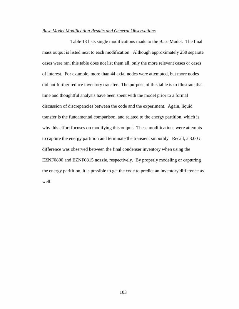
103
Base Model Modification Results and General Observations
Table 13 lists single modifications made to the Base Model. The final
mass output is listed next to each modification. Although approximately 250 separate
cases were ran, this table does not list them all, only the more relevant cases or cases
of interest. For example, more than 44 axial nodes were attempted, but more nodes
did not further reduce inventory transfer. The purpose of this table is to illustrate that
time and thoughtful analysis have been spent with the model prior to a formal
discussion of discrepancies between the code and the experiment. Again, liquid
transfer is the fundamental comparison, and related to the energy partition, which is
why this effort focuses on modifying this output. These modifications were attempts
to capture the energy partition and terminate the transient smoothly. Recall, a 3.00 L
difference was observed between the final condenser inventory when using the
EZNF0800 and EZNF0815 nozzle, respectively. By properly modeling or capturing
the energy paritition, it is possible to get the code to predict an inventory difference as
well.

104
Table 13. List of modifications to the Base Model and subsequent final
condenser inventory predicted by TRACE.
Modeling the pipe with the VESSEL component and adding non-
condensable gases will be discussed in detail later in this Chapter.
Changing the number of axial pipe nodes had little effect on final
inventory. For more than 44 nodes, the calculation began to take extremely long.
Slightly less final inventory is seen for 44 nodes, and all other parameters (pressure,
etc.) remain the same regardless of nodalizaton. Specifically, the discontinuous
pressure recovery is still present.
Enhancing the surface area of the pipe wall by using the N-RODS
parameter reduced the final inventory by approximately 0.25 kg. By enhancing the

105
surface area, we have enabled the code to capture a hint of the energy partition and
what occurs when a fan nozzle is used. More energy from the incoming spray being
transferred to cooling the wall (as opposed to collapsing the vapor space) resulted in
less inventory transfer and smaller final condenser inventory. Enhancing the surface
area in the model allows TRACE to preference more energy to the wall. No further
advantage was noted by enhancing the area more the 5X entry listed in the table.
Changing the wall material to copper (a user defined material with
better conduction characteristics than carbon steel) caused the code to progress
through approximately half the transient before abruptly terminating with a fatal
error.
Changing the wall material to insulation (a user defined material which
does not allow conduction) resulted in slightly more inventory transfer. This slight
increase is due to a slightly lower temperature profile. Making the wall insulated
commits all of the (negative) energy of the incoming spray to collapsing the vapor
space. Noting this enhanced inventory transfer and recalling that enhancing the
surface area of the metal decreased inventory transfer, lends credence to the idea of
the energy partition and the physics upon which it was based.
Changing the frictional losses in the copper tubing resulted in a slight
decrease in predicted final inventory. Exaggerating the losses to 5 or 10 times a
realistic value had little effect. Changing the friction factors in the tubing caused the
transient to last longer, but did little to reduce or prevent inventory transfer.
Changing the accumulator model from “no accumulator” to “falling
film” or “suppression pool” cause a slight decrease in predicted final condenser

106
inventory. “Falling film” forces TRACE to treat the incoming spray as a film falling
down the pipe wall, and modifies the way the code homogenizes the calculation node.
This modification is not significant enough to cause the large inventory differential
noted in the experiment.
Much like changing the losses in the copper, changing the nozzle
friction factor simply caused the transient to last longer, but did little to reduce or
prevent inventory transfer.
Non-condensable Gas Modifications to Base Model
Non-condensable gases are purged from the system by boiling the
inventory for 3 hours. Non-condensable gases are known to hinder condensation
(Uchida, 1965) and are stripped to ensure MANOTEA transients start properly and do
not terminate prematurely. Because a small amount (approximately 1% or 820 Pa, as
discussed in Chapter 7) of non-condensable is known to accumulate in DPHE, it was
suggested that gases should be added to the code in order to see what happens. When
a transient is initiated, these gases lead the sub-cooled water into the condenser. In
order to capture the effect of the gases and the appropriate concentration, the primary
side of the DPHE was model as being full of air at transient initiation.
As expected, the presence of non-condensable gases caused less liquid
inventory to be transferred during the simulated transient. It should be emphasized
again that the energy partition is responsible for this bulk effect in the MANOTEA
facility, but the presence of non-condensable gases does contribute slightly.
Although a small fraction, as the transient progresses and the condenser fills, the non-
condensable fraction becomes larger. Some of the gases are likely absorbed into the

107
relatively cool pooled water, while some remain in the vapor space. The increasing
concentration in the vapor space is eventually a contributing factor to transient
termination. In addition, the presence of non-condensable gases is posited to be one
of the reasons for the slight, smooth pressure recovery found at the end of all
MANOTEA transients.
Figure 54 shows an order of magnitude parametric study performed
with TRACE. The figure shows three plots: 50, 500, and 5000 Pa of non-
condensable gas in the condenser at transient initiation, respectively.

108
Figure 54. Parametric non-condensable gas study performed with TRACE.

109
Note that the times scales shown in Figure 54 are not the same, but the
pressure scales are the same. The figure illustrates the effects of non-condensable gas
in general. For large enough initial concentration, TRACE predicts that condensation
will be suppressed and transient initiation delayed. In addition, for larger
concentrations, the minimum pressure prediction is greater than for smaller
concentrations, again indicating reduced condensation. For a non-condensable
concentration on the order of our estimate for the MANOTEA facility, transient
termination begins to look like the experimental data (see Figure 10, 15, etc).
However, in all cases, pressure (and the shape of the pressure curve) at transient
initiation is slightly different from that observed in the data. Modeling the condenser
pipe with the VESSEL component eliminated this discrepancy, and will be discussed
more later in this Chapter.
VESSEL Modifications to Base Model
When employing finite difference analysis, one set of parameters is
associated with or characteristic of each cell or node. This feature has been referred
to as homogenization. The motivation for modeling the 1D condenser pipe with the
3D VESSEL component was to try to reduce the node size and force the energy
partition to occur.
Using the PIPE component to model the condenser forces the upper
portion of the condenser, where the sub-cooled spray enters, to be treat as one node.
Thus, the spray comes into the upper node and is homogenized in order to implement
finite-difference equations for mass, energy, and momentum. After calculations
haves been performed for this initial calculation node, it becomes the donor node for

110
a series of subsequent calculations, to include wall heat transfer. In this manner, it is
truly impossible to capture the effect of a fan nozzle and preference energy transfer
(the energy partition) to the wall while employing the PIPE component.
Figure 55 is an overheard view of the VESSEL component configured
with 11 axial nodes (not viewable in the figure), 2 radial ring nodes, and 1 azimuthal
sector node. Configuring the component in this way allows the energy partition to be
simulated. Incoming sub-cooled spray can be directed into the outer ring where it is
homogenized and finite-difference and constitutive equations solved. This node then
becomes the donor node for a calculation with the carbon-steel pipe wall on the
outside and a portion of the vapor space on the inside. In this manner, the spray is
allowed only to “communicate” with a smaller portion of the vapor space initially.
The subsequent calculations with the wall and the vapor space forces some of the
incoming (negative) energy to the wall, much like a fan nozzle exchanges a portion of
the energy directly with the wall. The presence of an extra step before the spray can
communicate with the wall means that the energy partition effect will be diminished
when compared to the effect observed in the experiment.

111
Figure 55. Top view of VESSEL component with 2 radial ring nodes and 1
azimuthal node.
As shown in Table 13, when incoming spray was directed into the
inner radial node, the resulting final condenser inventory is 28.86 kg. If the incoming
spray is directed into the outer radial node, the resulting final condenser inventory is
28.31 kg. Also note from Table 13, when the VESSEL is configured to 1 radial ring
node and 1 azimuthal node (essentially forcing the VESSEL to behave like a PIPE
component), the final condenser inventory matches that predicted with a PIPE
component configured with the same scheme and is 28.79 kg. Thus, when the spray
was forced into the vapor space and not allowed to communicate directly with the
wall, more pressure-volume work was done and more liquid inventory was
transferred. When the spray was forced to communicate with the wall by directing it
into the outer radial ring, less pressure-volume work was done and more quenching,
resulting in reduced liquid inventory transfer. This reinforces the validity of framing
MANOTEA transients in terms of an energy partition. Furthermore, using the

112
VESSEL component allows the energy partition to be recreated or captured in an
conclusive manner. Unfortunately, the inventory differences observed with TRACE
are not of the same magnitude as those observed with the EZNF08XX series
experiments. However, it does suggest that the TRACE condensation model is
overstated. This observation has been made for TRACE’s predecessors RELAP5 and
RELAP5 -3D in previous works as well (Woods, 2009; Moon, 2000; Choi, 2002).
Modeling the condenser as a VESSEL also resulted in better
agreement in the shape and slope of the pressure versus time plots – particularly at
transient initiation. These results are reasoned to be related to the ability of the
VESSEL component to better capture the small circulations cells described in
Chapter 7.

113
Chapter 13: Final TRACE Model
A Final Model of MANOTEA was created implementing relevant
modifications and lessons learned from the Base Model modifications exercise
outlined in Chapter 12. Namely, the Final Model incorporated two important
changes: add non-condensable gases in the DPHE at transient initiation and use of
the VESSEL component instead of the PIPE component to model the condenser pipe.
The adjective “final” is used not in the sense that the model is perfect, but in the sense
that enough information has been gathered to make recommendations. Accounting
for the small fraction of non-condensable gases eliminated the pressure discontinuity
predicted by the Base Model (one of the two fundamental discrepancies outlined
Chapter 11). Implementing the VESSEL component prevented the condenser from
filling – although not to the extent observed in the experiment - by capturing the
energy partition (the second fundamental discrepancy). However, VESSEL also
introduces a new discrepancy.

114
Nodalization Scheme
The Final Model condenser used 11 axial nodes, 1 radial ring node, and 1
azimuthal node. This nodalization scheme is recommended for modeling jet nozzles.
In order to capture the energy partition and better predict fan nozzle transients, the
condenser should simply be re-nodalized to have 2 or more radial rings as described
in Chapter 11. Renodalizing from 1 to 2 radial rings takes less effort than
renodalizing from 2 to 1 radial ring. Thus, the Final Model incorporated a VESSEL
component with 1 radial ring. Figure 56 shows the nodalization scheme, with heat
structures, for the Final Model.

115
Figure 56. Nodalization and heat structure scheme for the Final TRACE
Model of MANOTEA.

116
Fundamental Comparison
Because MANOTEA is an integral facility, the most important data point is
how much inventory has been transferred. Thus, the fundamental comparison
between the data and the TRACE models was condenser pressure as a function of
condenser inventory.
Figure 57 shows the Base and Final Model outputs for condenser pressure
versus condenser inventory. For reference, two sets of experimental data are also
plotted on the figure.
Figure 57. Fundamental comparison between MANOTEA data and TRACE
models.

117
The Base Model slightly over-predicted condenser pressure as a function of
condenser inventory. The Base Model was qualitatively and quantitatively accurate
to within experimental uncertainty, but failed to capture the pressure recovery during
transient termination. By adding non-condensable gas to the model in the appropriate
proportion, the Final Model was able to capture the pressure recovery to within
experimental uncertainty. However, the Final Model under-predicted condenser
pressure versus condenser inventory during the first half of the transient. Certain
portions of the early-transient behaviors predicted by the Final Model are outside of
experimental uncertainty. The lower-than-observed-pressures in the Final Model are
due to the VESSEL component modification. Regardless of nodalization, VESSEL
always under-predicted early pressure for all cases attempted. VESSEL allows 3D
fluid movement. The under-prediction is attributed to this feature and is likely due to
more fluid movement and heat convection than actually occurred in the highly linear,
thermally stratified condenser. The advantage to using VESSEL was that it provided
a mechanism to capture the energy partition and prevent the condenser from filling.
In this manner, using the VESSEL component is a trade-off.

118
Other One-to-one Comparisons
Pressure
Figure 58 is the Base and Final Model output for boiler and condenser
pressure as a function of time, respectively. TRACE qualitatively captured the
general pressure trends observed in the experiment. The Base Model quantitatively
captured condenser pressure, and predicted transient duration well. However, the
pressure slope predicted by the Base Model at transient initiation does not match the
experimental data well – the pressure plot seems to lag slightly behind what was
observed in the experiment. In addition, the Base Model predicted a non-physical
pressure discontinuity at transient termination. Again, by incorporating non-
condensable gases into the Final Model, this discontinuity is eliminated via
mechanisms explained in Chapter 7. However, as mentioned in the preceding
section, the Final Model under-predicted condenser pressure versus condenser
inventory during the first half of the transient. Both models predict two distinct
pressure regimes in the boiler, which was also noted in the experiment. However,
TRACE did not quantitatively capture boiler pressure. Because the present work is
focused on rapid condensation transients and MANTOEA transients are not affected
by the boiler, this discrepancy is considered minor and is left for future work.
Timescales on Figure 58 are tied to the code’s prediction for transient termination,
and are therefore different.

119
Figure 58. Base and Final Model output for pressure versus time after
transient initiation. Inset is qualitative snapshot of experimental data for quick
comparison.

120
Temperature
Figure 59 is the Base and Final Model outputs for condenser centerline
temperature as a function of time. Condenser surface temperatures are directly
related to condenser centerline temperatures and not shown in this section.
Timescales are again tied to transient termination.
Both models predicted the inverted thermal stratification observed in
the MANTOEA condenser. In addition, both captured the general trends. However,
the Base Model predicted slightly higher than experimentally observed temperatures.
The Final Model predicted lower than experimentally observed temperatures and
cooled much faster. These results are consistent with the pressure versus time
profiles predicted by both models, as well as the pressure versus inventory plots.

121
Figure 59. Base and Final Model output for condenser centerline temperature
versus time after transient initiation to transient termination. Inset is qualitative
snapshot of experimental data for quick comparison.

122
Inventory
Figure 60 is the Base and Final Model outputs for mass as a function
of time. Both models captured the qualitative trends. Inventory is transferred faster
in the Final Model prediction as a direct result of the lower temperatures and pressure
predicted during the early transient. Thus, these again are consistent with other
TRACE outputs for the respective models.
The models also showed quantitative agreement with the experimental
data. Recall, that the EZNF0815 nozzle (15-deg or fan nozzle), transferred
approximately 3.5 L less than the EZNF0800 nozzle (0-deg or jet nozzle) due to the
energy partition. The Base Model always predicted that the condenser will fill and
terminate with a pressure discontinuity. The Final Model predicted that the
condenser will fill and terminate smoothly when configured with default nodalization.
If re-nodalized radially to capture the energy partition, the Final Model will not fill
the condenser. Thus, a novel way to capture the energy partition in the model was
found. However, the using the VESSEL component introduced some new errors as
discussed in the first section of this Chapter. Unfortunately, the inventory differences
observed with TRACE are not to the extent as those observed with the EZNF08XX
series experiments.

123
Figure 60. Base and Final Model output for inventory versus time after
transient initiation to transient termination. Inset is qualitative snapshot of
experimental data for quick comparison.

124
Chapter 14: Analysis of Main Discrepancies and Anomalies
Before discussing discrepancies, it is fitting to summarize what the code
predicted well. The TRACE models predicted the following general trends or
phenomena to an acceptable degree:
- The qualitative nature of the fundamental comparison: condenser pressure as
a function of condenser inventory,
- The qualitative condenser pressure as a function of time,
- Inverted thermal stratification in the condenser pipe,
- Qualitative temperature as a function of time in the condenser,
- Qualitative boiler and condenser inventory as a function of time,
In addition, by choosing the model appropriate for a given nozzle geometry,
TRACE was able to:
- Capture the energy partition,
- Predict whether the transient continued until the condenser filled or
terminated before filling.
For the most part, the TRACE models were able to bracket the quantitative
nature of the transient variables, with the Base Model providing the upper boundary
and the Final Model providing the lower. The condenser always filled when using
the PIPE component in the Base Model. By using the VESSEL component in the
Final Model, the condenser filling could be prevented but never to the extent
observed in the experiment. All other plots (pressure vs. time, temperature vs. time,

125
etc.) supported these final inventory predictions and presented a consistent story
throughout. Although consistent, the TRACE predictions were qualitatively different
from the data. All discrepancies between the experiment and model predictions can
be summarized as originating in an over-stated condensation model, as discussed in
Chapter 12. Due to the consistent nature of the TRACE predictions, discrepancies
can be treated as a subset of the fundamental comparison.
Over-stated Condensation Model
Difference between Data and Model
In the Base Model, TRACE always predicted that the condenser would
fill and terminate the transient with a pressure discontinuity. The discontinuity was
eliminated in the Final Model by adding a small fraction of non-condensable gas,
which initially did little to affect rapid condensation but eventually provided an
amplifying mechanism to terminate the transient smoothly. The Final Model
prevented the condenser from filling by nodalizing a VESSEL component radially to
capture the energy partition. In doing so, a transient simulated with the Final Model
predicted approximately 0.5 L less than a transient simulated with the Base Model.
Experimental data showed that transients ran with the EZNF0815 nozzle (15-deg or
fan nozzle) transferred approximately 3.5 L less than the EZNF0800 nozzle (0-deg or
jet nozzle) due to the energy partition. TRACE consistently transferred more
inventory than experimentally observed, suggesting that the code’s condensation
model is over-stated.

126
Implications
An over-stated condensation model means that TRACE will amplify
or over-predict condensation-induced fluid motion when modeling the following
reactor situations/systems:
- Water slug delivery in an annular downcomer,
- Steam discharge into large pools of sub-cooled water like those found in a
suppression tank,
- Cold leg oscillations induced by ECC injection,
- Reflux condensation oscillations in U-tube steam generators,
- Oscillations due to combined injection of ECC liquid into both the hot and
cold legs,
- Heat and mass transfer due to small pressure and temperature driving forces.
An accurate prediction of the condensation-induced fluid motion in
these situations is imperative for the safe regulation and operation of both current and
future light-water reactor systems. Over-stated condensation means that TRACE will
predict fluid is present in a system or situation when it isn’t, or vice versa. The
absence of fluid when it was expected to be there is a serious concern.
Possible Source of Discrepancy
TRACE uses models or empirical correlations to solve for heat
transfer coefficients and subsequently solve constitutive or balance equations as
needed. The code is capable of estimating coefficients for direct contact, drop-wise,
and both laminar and turbulent film condensation. TRACE uses typical heat transfer
and fluid dynamic qualifiers like void fraction, Reynolds number, and Nusselt

127
number to determine the appropriate type of condensation correlation to perform the
calculation. Film condensation is the default mode (Applied Programming
Technology, 2007b).
Each of the empirical correlations has applicable ranges, conditions,
and inherent uncertainties. These uncertainties are reasoned to be the primary source
of the discrepancies. Recommendations for improvements to the code, such as Batet
(2001), Choi (2002), Moon (2000), and Woods (2009), typically focus on adding
options to use a different correlation or modifying the code to use improved
correlations for a given experiment. For example, TRACE commonly uses the
Uchida correlation for condensation in the presence of non-condensable gases.(APT,
2007b; Massoud, 2005). However, to improve the predictive capabilities of the
TRACE code for the Passive Containment Cooling System of the proposed ESBWR,
the developers modified the code to employ the mass transfer conductance approach
developed by Kuhn and co-workers (1994). Once a modification like this is made,
the challenge is to ensure that the change is still capable of predicting all the other
phenomena correctly – that is: nothing else should be adversely affected by the
change. In the case of the Kuhn approach, the NRC subsequently performed analysis
and ultimately compared the TRACE output to the Uchida correlation. The
modification was able to predict the Uchida data (APT, 2007b). However, if the
Uchida correlation over or under-predicts experimental data, TRACE must obviously
over or under-predict for the same data. This short discussion also suggests why
RELAP5 would over-predict condensation, and its offspring, TRACE, still over-
predicts condensation: the evolution process is complex and robust.

128
Possible Solution
The Base and Final Models bracketed the transient well, and in some
cases the predictions were within the uncertainty of the experiment. Thus, the code
performed well in predicting MANOTEA transient behaviors. The condensation
model is over-stated, but not grossly so.
In the MANOTEA condenser there is a mix of direct condensation
with sub-cooled droplets in the vapor space and film condensation on the wall.
Because the vapor space and wall are both relatively warm, there is also vaporization
in the vapor space and the wall. Rather than choosing a better correlation or
modifying the present correlations invoked by the code to better capture MANOTEA
behavior, it is suggested that a NOZZLE component could be developed for TRACE.
Currently, nozzles are modeled using the FILL component and
assigning a loss coefficient. In some cases, the take-off angle can also be used to help
capture some nozzle characteristics. While the FILL component captures the pressure
and velocity changes associated with liquid moving through a nozzle, it does not
capture the nozzle geometry effects. In a large reactor pressure vessel, these
geometry effects could be argued to be negligible. But, in the high aspect ratio pipe
like the MANOTEA condenser, these effects become very important. Spray
geometry affects the energy partition, which subsequently dictates how much rapid
condensation-induced liquid inventory is transferred. A nozzle component could
prove useful and greatly simplify modeling of numerous transients.

129
The TRACE Theory Manual (Applied Programing Technology,
2007b) mentions that developers are working on a droplet field to improve re-flood
and spray models. This droplet field could prove useful in improving MANOTEA
simulations. The NRC has had an active role in this project, and developers are
familiar with the results. As a consequence, the NRC is working on an implicit
nozzle model (Staudenmeier, 2011). Merging the spray field and nozzle model work
into a single, comprehensive NOZZLE component could greatly improve agreement
between TRACE predictions and MANOTEA data by providing an easy means to
capture the energy partition and ensure the appropriate mix of film and direct
condensation is occurring.

130
Chapter 15: Modeling Summary
A 1-dimensional Base Model was developed prior to the termination of the
experimental phase. Since TRACE is used to make regulatory decisions about the
safety of proposed designs, this model was intentionally developed in this manner in
order to provide unique insight. Output from the Base Model was eventually
compared to experimental data and found to over-estimate the pressures and
temperatures observed in the experiment. In addition, this model always predicted
that the condenser pipe would fill, and that transients would terminate with a non-
physical discontinuity.
A list of the phenomena and their ability to affect the transient was generated,
and then mapped to TRACE parameters that could be used to exaggerate or reduce
the effect of the relevant phenomena. In general, this exercise was aimed at finding
valid ways to capture the energy partition, and in doing so, prevent the condenser
from filling. Over 250 TRACE cases were run, and the effective and physically
justifiable parameters were incorporated into a 3-dimensional Final TRACE Model.
The Final Model incorporated the effects of non-condensable gases, which provided a
mechanism by which transients could terminate smoothly and better match the data.
Replacing the PIPE component in the Base Model with a radially nodalized VESSEL
component in the Final Model, provided an undeniable way to model the energy
partition and prevent the condenser from filling.

131
Whereas the Base Model generally over-predicted parameters, the Final
Model generally under-predicted trends observed in the experiments. Thus, the 2
models were able to bracket the fundamental comparison, condenser pressure versus
condenser inventory, and other trends observed during the experimental phase. By
providing an upper and lower bound, TRACE was deemed capable of effectively
modeling integral, rapid-condensation transients.
Thoughtful comparison of the TRACE output to the data led to the conclusion
that the condensation model used by the code is over-stated. The code’s
predecessor’s, TRAC and RELAP, where also known to have over-stated
condensation models. An over-stated condensation model means that TRACE will
amplify or over-predict condensation-induced fluid motion when modeling several
common thermal-hydraulic reactor situations important to safe reactor operation.
The TRACE Theory Manual mentions that developers are working a droplet
field to improve re-flood and spray models. This droplet field could prove useful in
improving simulations of rapid-condensation transients from MANOTEA. The NRC
is also working on an implicit nozzle model. Merging the spray field and nozzle
model work into a single, comprehensive NOZZLE component could greatly improve
agreement between TRACE predictions and MANOTEA data by providing an easy
means to capture the energy partition and ensure the appropriate mix of film and
direct condensation are occurring.

132
Chapter 16: Conclusions and Recommendations
Conclusions
The purpose of the present work was to experimentally validate the TRACE
(TRAC-RELAP Advanced Computational Engine) plug-in for the Nuclear
Regulatory Commission’s (NRC’s) Symbolic Nuclear Analysis Package (SNAP) for
rapid condensation transients. The TRACE plug-in is designed to analyze thermal-
hydraulic transients in light water reactors. The challenges that integral,
condensation-driven transients have posed to thermal-hydraulic codes provided the
motivation for the present work. The present work is particularly relevant because
many of the proposed passive mechanisms and safety systems found in next
generation reactors rely on rapid condensation for normal operation or accident
mitigation.
The present work was undertaken in two phases: an experimental and
modeling phase. Data obtained during the experimental phase was subsequently
compared to output from a Base TRACE (TRAC-RELAP Advanced Computational
Engine) model. Discrepancies between the data and the code output were used to
identify potential problem areas in the code, and the improvements where used to
generate a Final TRACE model. Comparisons between the models and the data
provided a basis for recommendations for potential ways to improve TRACE for
condensation-driven transients.
133
The experimental phase began by constructing and calibrating a simplified,
integral, condensation-driven transient apparatus named the UMD-USNA Near One-
dimensional Transient Experimental Assembly (MANOTEA). MANOTEA was
designed to create rapid condensation transients. The facility is deemed simple
enough that human intuition and simple models can still predict transient behavior,
yet complex enough to provide a meaningful challenge and validation for the TRACE
code.
After calibration, shake-down, and scoping experiments were ran, a series of 5
well-defined transient experiments were ran on MANOTEA and the data analyzed.
Each transient was run twice to verify repeatability. Raw, standalone data from the
facility included: pressure, differential pressure, and temperature profiles, all as a
function of time. Using the raw data, a mass and energy balances were closed for
each of the experiments. Some of the relevant characteristics of the data included:
inverted thermal stratification in the condenser and nozzle dependent transients that
are physically controlled by an energy partition. Plotting pressure as a function of
inventory revealed a convenient way to summarize all of the transient datasets and
resulted in a transient sequence. This sequence highlighted the integral nature of
MANOTEA transients and ties the facility to more complex reactor systems. The
transient sequence, which was a plot of condenser pressure versus condenser
inventory, served as the fundamental comparison to evaluate TRACE during the
second phase of the present work. The first phase terminated with the end of the
experiments.

134
The second phase began by developing a 1-dimensional Base TRACE Model.
The Base Model was developed prior to the termination of the experimental phase.
Since TRACE is used to make regulatory decisions about the safety of proposed
designs, this model was intentional developed in this manner in order to provide
unique insight. Output from the Base Model was eventually compared to
experimental data and found to over-estimate the pressures and temperatures
observed in the experiment. In addition, this model always predicted that the
condenser pipe would fill, and that transients would terminate with a non-physical
discontinuity.
A list of the phenomena and their ability to affect the transient was generated,
and then mapped to TRACE parameters that could be used to exaggerate or reduce
the effect of the phenomena. In general, this exercise was aimed at finding unique
ways to capture the energy partition, and in doing so, prevent the condenser from
filling. Over 250 TRACE cases were run, and the effective and physically justifiable
parameters were incorporated into a 3-dimensional Final TRACE Model. The Final
Model incorporated the effects of non-condensable gases, which provided a
mechanism by which transients could terminate smoothly and better match the data.
Replacing the PIPE component in the Base model with a radially nodalized VESSEL
component in the Final Model, provided an undeniable way to model the energy
partition and prevent the condenser from filling. Whereas the Base model generally
over-predicted parameters, the Final Model generally under-predicted trends observed
in the experiments. Thus, the 2 models were able to bracket the fundamental
comparison, condenser pressure versus condenser inventory.

135
Thoughtful comparison of the TRACE output to the data led to the conclusion
that the condensation model used by the code is over-stated. The code’s
predecessor’s, TRAC and RELAP, where also known to have over-stated
condensation models. An over-stated condensation model means that TRACE will
amplify or over-predict condensation-induced fluid motion when modeling several
common thermal-hydraulic reactor situations important to safe reactor operation.
Recommendations and Future Work
The TRACE Theory Manual mentions that developers are working a droplet
field to improve re-flood and spray models. This droplet field could prove useful in
improving simulations of rapid-condensation transients from MANOTEA.
Throughout the present work, the NRC has had an active role and developers are
familiar with the results. As a consequence, the NRC is working on an implicit
nozzle model. Merging the spray field and nozzle model work into a single,
comprehensive NOZZLE component could greatly improve agreement between
TRACE predictions and MANOTEA data by providing an easy means to capture the
energy partition and ensure the appropriate mix of film and direct condensation are
occurring.
Future work could focus on developing a NOZZLE component and comparing
the subsequent TRACE output to MANOTEA data. Should this effort prove
successful, other nozzle situations could be modeled for comparison to other datasets.
The boiler pipe was of minor concern to the present work, but data from the
MANOTEA experiments could be used to draw conclusions about TRACE’s flashing
models. Further experiments with MANOTEA in the current configuration are of

136
little use as previously mentioned. However, the facility could be modified to use
larger copper tubing in the DPHE. This could create a situation in which the flashing
in the boiler and condensation in the condenser pipe are competing to control
transient behavior. Data from this modified facility could then be compared to a new
TRACE model and may provide some new insight.

137
APPENDICES

138
Appendix A: Experimental Procedures Checklist
The following is a detailed, itemized list of steps outlining how to prepare the
facility and run a transient:
Procedures to Prepare for Transient
- Reboot computer and verify data acquisition system (DAQ) is
functional
- Open tee valves at the top of the boiler and condenser pipe to vent
to atmosphere
- Close valve on the bottom of the boiler that allows inventory to
flow from the boiler directly to the condenser
- Open valve on the bottom of the boiler that allows inventory to
flow from the boiler into the double-pipe heat exchanger (DPHE)
- Install brass cap on the tee in the tubing that connect the boiler
directly to the condenser
- Open valve on the bottom of the condenser that allows inventory to
flow from the condenser directly to the boiler
- Zero strain gauges and pressure transducers
- Begin temperature, pressure, and strain logging on DAQ
- Open solenoid valve that isolates primary inventory from
condenser pipe
- Remove plug from the fill hole at the top of boiler
- Fill boiler with water
- Close solenoid valve

139
- Close the valve at the bottom of the boiler to isolate the boiler from
the DPHE
- Open valve at the bottom of the boiler to allow inventory to flow
from the boiler directly to the condenser
- Wait for water to settle to 50/50 (half in the boiler and half in the
condenser)
- Add 3.79 L (1 U.S. gallon) of water to the total inventory via the
fill hole
- Install fill hole plug
- Turn boiler and condenser heaters to full power
- Heat inventory in both pipes for about 3 hours in order to de-gas
- Turn off boiler heater
- Close tee valve at the top of condenser isolating it from the
atmosphere and opening it to the condenser pressure transducer
- Monitor condensing pressure and continue heating condenser side
until water just spills out of the tee valve on the top of the boiler
- Close tee valve at the top of the boiler isolating it from the
atmosphere and opening it to the boiler pressure transducer
- Shut off condenser heater and unplug
- Close valves at the bottom of the boiler and condenser to isolate
them from each other and prevent inventory from flowing directly
between them
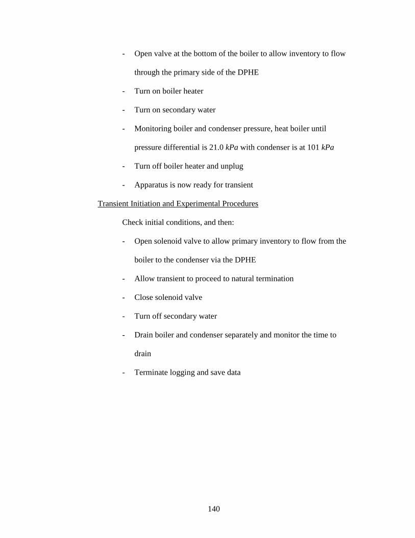
140
- Open valve at the bottom of the boiler to allow inventory to flow
through the primary side of the DPHE
- Turn on boiler heater
- Turn on secondary water
- Monitoring boiler and condenser pressure, heat boiler until
pressure differential is 21.0 kPa with condenser is at 101 kPa
- Turn off boiler heater and unplug
- Apparatus is now ready for transient
Transient Initiation and Experimental Procedures
Check initial conditions, and then:
- Open solenoid valve to allow primary inventory to flow from the
boiler to the condenser via the DPHE
- Allow transient to proceed to natural termination
- Close solenoid valve
- Turn off secondary water
- Drain boiler and condenser separately and monitor the time to
drain
- Terminate logging and save data

141
Appendix B: Clausius-Clapeyron Primer
The Clausius-Clapeyron equation allows the change in enthalpy during
vaporization, sublimation, or melting at a constant temperature to be evaluated from
pressure/specific volume/temperature data pertaining to the phase change. In short, it
provides a pressure-temperature relationship for saturated states. The equation can be
written as:
(dp/dT)sat = (hg – hf)/(RT2/p)
Letting Λ = (hg – hf), noting that Λ/RT ~ constant (a small change in T results in a
large change in p), and separating the variables:
(1/p)dpsat = (Λ/RT)(1/T)dT
Integrating both sides, we obtain:
ln(p) = (Λ/RT)(ln(T)) or p = TΛ/RT
Note for p = po and T = To, we can write:
po = To Λ/RT and (p/po) = (T/To)
Λ/RT
Letting Π = p/po, Θ = T/To, and CC = Λ/RT:
Π = ΘCC
The constant, CC, can be adjusted in order to fit data to pressure-temperature data,
such as small portions of the steam tables. Figure A.1 shows a fit for CC = 13.3.

142
Figure A.1. Curve Fit of Clausius-Clapeyron Equation to Steam Table Data (for
CC = 13.3).

143
Appendix C: Integral Energy Balance Assumptions
The following assumptions were used to simplify derivation of the integral
energy balance. Although many of these assumptions proved false, using them
enabled the derivation of an express that captured the energy partition and matched
the data fairly well.
Assumption 1: Pool is well mixed.
Combination of momentum from incoming jet, bubble/vapor generation in the
pooled liquid by energy transferred from the metal masses (pipe walls), and natural
convection currents ensures the pool is well mixed.
Note: MANOTEA data shows that this assumption is invalid.
Nonetheless, it is accepted axiomatically in order to ease energy balance derivation
and for clarity during early derivation. The energy balance is subsequently modified
in order to account for the lack of mixing.
Assumption 2: Vapor contribution to energy balance is small.
Energy in the vapor at transient initiation:
Eg = (0.598 kg/m3)(0.0274 m3)(2510 kJ/kg)
Energy in metal at transient initiation:
Em = (7850 kg/m3)(0.0105 m3)(0.490 kJ/kg*K)(100 K)
Energy in pool at transient initiation:
Ef = (958 kg/m3)(0.00379 m3)(419 kJ/kg)
Eg/(Eg + Em + Ef) = [41.0/(41.0 + 4040 + 1520)] = 0.00732 or 0.7% of
total energy in the system is in the vapor at transient initiation

144
A combination of low available energy and poor means to transport it ensures
that the vapor contribution is small. As the transient proceeds, vapor volume is
reduced. Thus, the contribution starts small and only gets smaller.
Assumption 3: Energy in metal mass is primarily transferred to the pooled liquid.
Energy transferred by 1-D conduction: Q/A = -k(dT/dx) W/m2
Energy transferred by convection: Q/A = h(Tm – Tf) W/m2
Initial ratio of energy transferred to the pool to total energy transfer:
[(0.187 m2)(60.0 W/ m2 K)(5K) + (0.187 m2)(51 W/mK)(5K)/(0.00635 m)] /
[(1.35 m2)(0.00246 W/mK)(5K)/(0.0381m) + (1.35 m2)(1.50 W/ m2 K)(5K) +
(0.187 m2)(60.0 W/ m2 K)(5K) + (0.187 m2)(51 W/mK)(5K)/(0.00635 m)] =
7565 W / 7576 W = 0.999 or 99+% of the heat transfer occurs between the
metal wall and the pool. As wetted area increases, this percentage increases.

145
Appendix D: Obtaining Energy Balance Parameters from Data
MANOTEA Integral Energy Balance:
P = e ∫0t{[0.00039 χ (dTm/dt) – 1.8(d(fVL )/dt)] / fVL} dt
dVL/dt is obtained from a plot of the instantaneous (spray) volumetric flow rate as a
function of time. Figure A.2 is an example. This plot is generated by applying the
manufacturer’s nozzle equation using data gathered by the differential pressure cell.
This data is fed directly into the equation above in a spreadsheet.
Figure A.2. Instantaneous volumetric flow rate as a function of time.
VL is obtained by summing the instantaneous volumetric flow rate over time. A result
is shown in Figure A.3.

146
Figure A. 3. Volume as a function of time.
dTm/dt is obtained by applying a curve fit to condenser pipe temperatures as a
function of time. This technique is shown in Figure A.4.
Figure A.4. Change metal temperature as a function of time.

147
χ and f could theoretically be obtained from the experimental data. However, this is
considered tedious and beyond the scope of the present work, since the purpose of the
energy balance derivation was simply to prove understanding of the physics involved
during transient progression.

148
Appendix E: TRACE Terminology
The following general, pertinent terms are defined here for clarity: Mathematical model: refers to the application of the balance equations (and
equations of state if needed) to represent a physical phenomena.
Computational cell: a control volume for which the physical phenomena are
considered and mathematical models are developed.
Node: is the same as a computational cell. Divide a pipe of length L in into N pieces,
and the pipe would now be said to have N nodes of length L/N. Each node is
associated with a state that describes that node regardless of its size and shape. Thus,
each node has only a single temperature (and potentially a single case of other
appropriate properties/parameters) associated with it. This temperature is generally
taken to be the temperature at the center of the node. If more information about the
temperature distribution within an individual node is required, the system would have
to be re-nodalized.
Nodalization: in order to determine the state parameters, a system is broken down
into several nodes. This process is generally referred to as nodalization.
Control volume: a region of space through which mass/energy flows. A control
volume is used to simplify engineering analysis and is usually denoted by a dashed
line. Mass/energy is allowed to cross this dashed line which is known as a boundary
or system boundary. Control volume pressure and temperature are associated with
the center of the volume or node. Control volume velocity (momentum) is associated
with the volume’s edge or junction.

149
Junction(s): a flow path that allows separate nodes to communicate. Mass and
energy control volumes are connected together by junctions.
Donor cell: the “upstream” node or cell whose properties are used as input for the
calculation of the present cell’s properties.
Component: a physical piece of equipment represented symbolically in the analysis
code. Thermal-hydraulic components include: pipe, tee, valve, pump, etc. Each
component can be nodalized or divided into cells. Conservation equations are solved
for each cell and passed “downstream”. A component is a pre-packaged, but
configurable model of common physical structures.
Homogeneous Equilibrium Model (HEM): refers to the treatment of fluid in a
computational cell. Assumes liquid and vapor in a given cell are in thermal
equilibrium and that both phases flow with the same velocity.
Separated Equilibrium Model (SEM): refers to the treatment of fluid in a
computational cell. Assumes liquid and vapor in a given cell are in thermal
equilibrium but that each phase travels with a different velocity.
Two-fluid Model: refers to the treatment of fluid in a computational cell. Assuming
only liquid and vapor exist in a given computational cell, ten conservation equations
(1 conservation of mass for each phase, 1 conservation of energy for each phase, & 3
conservation of momentum equations for each phase) are used to describe the
conditions in that cell in terms of 10 unknowns (P, Tl, Tv, vxl, vyl, vzl, vxv, vyv, vzv, & α) .
Thus, in this mathematical model, water and steam can be at different temperatures
and flowing with different velocities.

150
Input Deck: a model comprised of all the physical components contained in an
apparatus and meant for simulation and analysis of phenomena with a code.

151
Appendix F: Conservation Equations in Finite Difference Form
The semi-implicit one-dimensional finite-difference equations for the mass,
energy, and momentum as implemented in TRACE are shown below. Note, these
equations are the same as or similar to those used in legacy codes such as RELAP and
TRAC. Some of the terms are intermediate time variables, which are denoted with a
tilde (~). Due to the complexity of the equations, they were captured as pictures from
the Code Manual (Applied 2007a & 2007b) and directly inserted here. All variables
have standard thermal-hydraulic meanings. Three dimensional versions of these
equations are available in the reference.
The sum continuity equation:
The difference continuity equation:
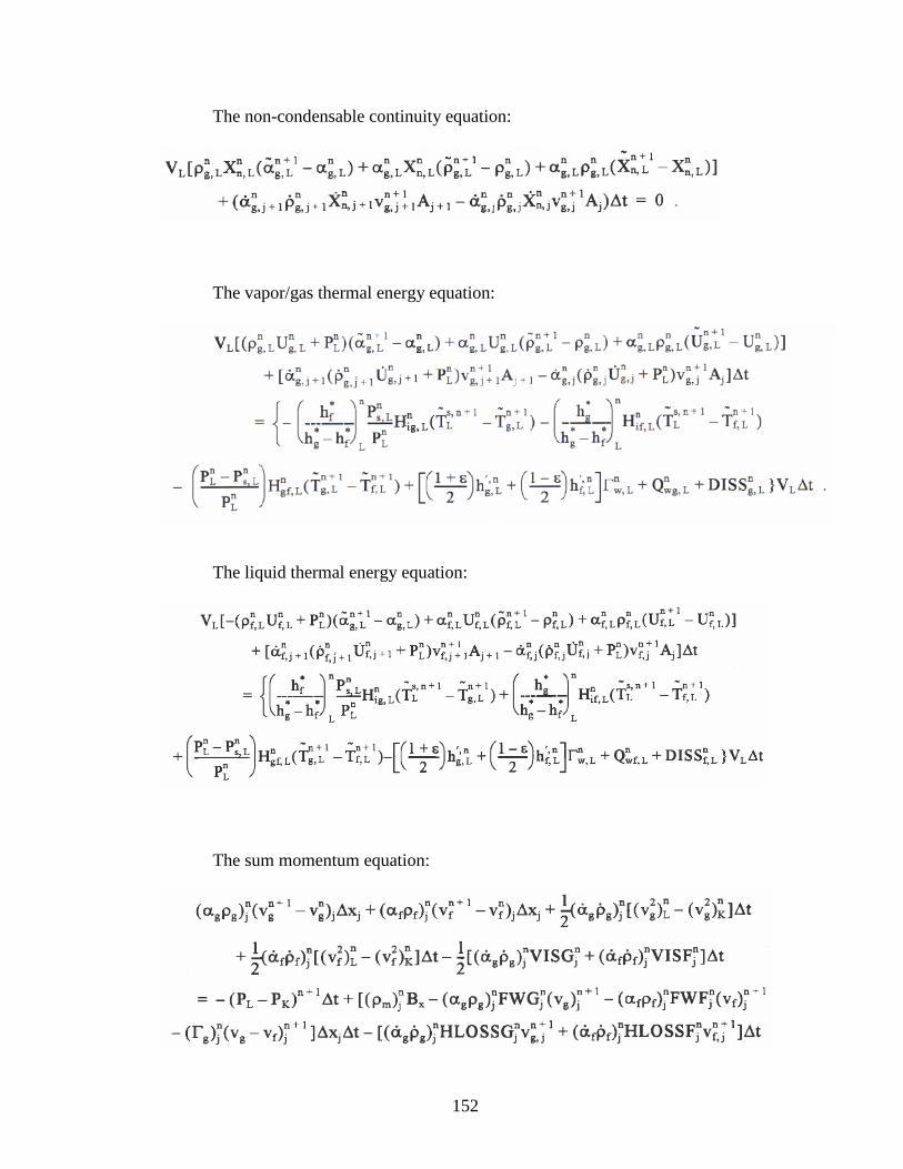
152
The non-condensable continuity equation:
The vapor/gas thermal energy equation:
The liquid thermal energy equation:
The sum momentum equation:

153
The difference momentum equation:

154
Appendix G: TRACE Input Decks
Note all TRACE modeling/coding was performed using the SNAP GUI.
However, for completeness, the input decks were exported to text in order to facilitate
those who are used to working with text input.
Base Model Input Deck
* * ************* * main data * ************* * * numtcr ieos inopt nmat id2o 1 0 1 3 0 * * ***************** * namelist data * ***************** * &inopts dtstrt=1.0, ikfac=1, ioinp=0, noair=0, usesjc=3, nhtstr=6 &end * *************** * Model Flags * *************** * * dstep timet 0 0.0 * stdyst transi ncomp njun ipak 0 1 16 8 1 * epso epss 1.0E-4 1.0E-4 * oitmax sitmax isolut ncontr nccfl 10 10 0 0 0 * ntsv ntcb ntcf ntrp ntcp 23 1 0 0 0 * ************************* * component-number data * ************************* * * Component input order (IORDER) *-- type ---- num ------------- name ---------------- + jun1 jun2 jun3 * PIPE * 1 s * Condenser + 0 32 * PIPE * 11 s * Boiler + 27 0 * PIPE * 21 s * CCDPHE Primary + 28 29 * PIPE * 31 s * CCDPHE Secondary + 31 1 * FILL * 51 s * Hose Inlet + 1 * BREAK * 61 s * Hose Outlet + 31 * HTSTR * 101 s * + * PIPE * 111 s * Lower BOP + 27 28 * PIPE * 112 s * Upper BOP + 26 23 * HTSTR * 121 s * +

155
* HTSTR * 122 s * + * PIPE * 131 s * Nozzle + 23 32 * HTSTR * 132 s * + * HTSTR * 141 s * + * VALVE * 151 s * + 29 26 * HTSTR * 161 e * + * *********************** * material properties * *********************** * * matb* 50 51 52 e * ptbln* 1 1 1 e * User Defined Material : 50 * *n: Copper Alloy * *d: Copper Alloy * prptb temp rho cp cond emis * prptb* 293.0 8940.6 385.0 394.0 0.0 e * * User Defined Material : 51 * *n: PVC * * prptb temp rho cp cond emis * prptb* 293.0 1390.0 900.0 0.16 0.0 e * * User Defined Material : 52 * *n: Insulation * * prptb temp rho cp cond emis * prptb* 293.0 48.05539 670.0 0.033172414 0.0 e * * * ************************************************** * Starting Signal Variable Section of Model * ************************************************** *n: Boiler Pressure * * idsv isvn ilcn icn1 icn2 1 21 11 3 0 *n: CC19 * * idsv isvn ilcn icn1 icn2 2 23 1 10 0 *n: CC11 * * idsv isvn ilcn icn1 icn2 3 23 1 6 0 *n: CC15 * * idsv isvn ilcn icn1 icn2 4 23 1 8 0 *n: CC07 * * idsv isvn ilcn icn1 icn2 5 23 1 4 0 *n: CC13 * * idsv isvn ilcn icn1 icn2 6 23 1 7 0 *n: CC09 * * idsv isvn ilcn icn1 icn2 7 23 1 5 0 *n: CC03 * * idsv isvn ilcn icn1 icn2

156
8 23 1 2 0 *n: CC21 * * idsv isvn ilcn icn1 icn2 9 23 1 11 0 *n: CC17 * * idsv isvn ilcn icn1 icn2 10 23 1 9 0 *n: CC05 * * idsv isvn ilcn icn1 icn2 11 23 1 3 0 *n: CC01 * * idsv isvn ilcn icn1 icn2 12 23 1 1 0 *n: BC21 * * idsv isvn ilcn icn1 icn2 13 23 11 3 0 *n: BC11 * * idsv isvn ilcn icn1 icn2 14 23 11 2 0 *n: BC01 * * idsv isvn ilcn icn1 icn2 15 23 11 1 0 *n: Primary Inlet * * idsv isvn ilcn icn1 icn2 16 23 51 1 0 *n: Primary Outlet * * idsv isvn ilcn icn1 icn2 17 23 61 1 0 *n: Condenser Pressure * * idsv isvn ilcn icn1 icn2 24 21 1 11 0 *n: Boiler Inventory * *d: FlashLevel * idsv isvn ilcn icn1 icn2 25 124 11 0 0 *n: Boiler Initial Inventory * *d: FlashIntLevel * idsv isvn ilcn icn1 icn2 26 125 11 0 0 *n: Condenser Initial Inventory * *d: CondeIntLevel * idsv isvn ilcn icn1 icn2 27 125 1 0 0 *n: Condenser Inventory * *d: CondeLevel * idsv isvn ilcn icn1 icn2 28 124 1 0 0 *n: Timer * * idsv isvn ilcn icn1 icn2 30 0 0 0 0 ************************************************** * Finished Signal Variable Section of Model * ************************************************** * * *

157
* ********************************************* * Starting Control System Section of Model * ********************************************* * ****** Control Blocks ****** *n: PressDif * *d: PressDif * idcb icbn icb1 icb2 icb3 -1 44 1 24 0 * cbgain cbxmin cbmax cbcon1 cbcon2 1.0 -1.0E20 1.0E20 0.0 0.0 * ********************************************* * Finished Control System Section of Model * ********************************************* * * * * ******* type num userid component name pipe 1 0 Condenser * ncells nodes jun1 jun2 epsw 11 0 0 32 0.0 * nsides 0 * ichf iconc pipetype ipow npipes 1 0 0 0 1 * radin th houtl houtv toutl 0.0 0.0 0.0 0.0 0.0 * toutv pwin pwoff rpwmx pwscl 0.0 0.0 0.0 0.0 0.0 * dx * 0.58181818 0.58181818 0.58181818 0.58181818s * dx * 0.58181818 0.58181818 0.58181818 0.58181818s * dx * 0.58181818 0.58181818 0.58181818e * vol * 2.6533E-3 2.6533E-3 2.6533E-3 2.6533E-3s * vol * 2.6533E-3 2.6533E-3 2.6533E-3 2.6533E-3s * vol * 2.6533E-3 2.6533E-3 2.6533E-3e * fa * 4.56037E-3 4.56037E-3 4.56037E-3 4.56037E-3s * fa * 4.56037E-3 4.56037E-3 4.56037E-3 4.56037E-3s * fa * 4.56037E-3 4.56037E-3 4.56037E-3 2.63022E-6e * kfac * 0.0 0.0 0.0 0.0s * kfac * 0.0 0.0 0.0 0.0s * kfac * 0.0 0.0 0.0 3.42e * grav * 1.0 1.0 1.0 1.0s * grav * 1.0 1.0 1.0 1.0s * grav * 1.0 1.0 1.0 1.0e * hd * 0.0762 0.0762 0.0762 0.0762s * hd * 0.0762 0.0762 0.0762 0.0762s * hd * 0.0762 0.0762 0.0762 1.83E-3e * nff * 1 1 1 1s * nff * 1 1 1 1s * nff * 1 1 1 1e * alp * 0.0 0.65 1.0 1.0s * alp * 1.0 1.0 1.0 1.0s * alp * 1.0 1.0 1.0e * vl * 0.0 0.0 0.0 0.0s * vl * 0.0 0.0 0.0 0.0s * vl * 0.0 0.0 0.0 0.0e * vv * 0.0 0.0 0.0 0.0s * vv * 0.0 0.0 0.0 0.0s * vv * 0.0 0.0 0.0 0.0e * tl * 378.0 378.0 378.0 378.0s * tl * 378.0 378.0 378.0 378.0s * tl * 378.0 378.0 378.0e * tv * 378.0 378.0 378.0 378.0s * tv * 378.0 378.0 378.0 378.0s * tv * 378.0 378.0 378.0e * p * 1.013E5 1.013E5 1.013E5 1.013E5s * p * 1.013E5 1.013E5 1.013E5 1.013E5s

158
* p * 1.013E5 1.013E5 1.013E5e * pa * 0.0 0.0 0.0 0.0s * pa * 0.0 0.0 0.0 0.0s * pa * 0.0 0.0 0.0e * * ******* type num userid component name pipe 11 0 Boiler * ncells nodes jun1 jun2 epsw 3 0 27 0 0.0 * nsides 0 * ichf iconc pipetype ipow npipes 1 0 0 0 1 * radin th houtl houtv toutl 0.0 0.0 0.0 0.0 0.0 * toutv pwin pwoff rpwmx pwscl 0.0 0.0 0.0 0.0 0.0 * dx * 2.1333333 2.1333333 2.1333333e * vol * 9.72878E-3 9.72878E-3 9.72878E-3e * fa * 3.16692E-5 4.56037E-3 4.56037E-3 4.56037E-3e * kfac * 0.49 0.0 0.0 0.0e * grav * 1.0 1.0 1.0 1.0e * hd * 6.35E-3 0.0762 0.0762 0.0762e * nff * 1 1 1 1e * alp * 0.0 0.0 0.0e * vl * 0.0 0.0 0.0 0.0e * vv * 0.0 0.0 0.0 0.0e * tl * 378.149 378.149 378.149e * tv * 378.149 378.149 378.149e * p * 1.209E5 1.209E5 1.209E5e * pa * 0.0 0.0 0.0e * * ******* type num userid component name pipe 21 0 CCDPHE Primary * ncells nodes jun1 jun2 epsw 3 0 28 29 0.0 * nsides 0 * ichf iconc pipetype ipow npipes 1 0 0 0 1 * radin th houtl houtv toutl 0.0 0.0 0.0 0.0 0.0 * toutv pwin pwoff rpwmx pwscl 0.0 0.0 0.0 0.0 0.0 * dx * 2.1333333 2.1333333 2.1333333e * vol * 6.7561E-5 6.7561E-5 6.7561E-5e * fa * 3.16692E-5 3.16692E-5 3.16692E-5 3.16692E-5e * kfac * 0.0 0.0 0.0 0.0e * grav * 1.0 1.0 1.0 1.0e * hd * 6.35E-3 6.35E-3 6.35E-3 6.35E-3e * nff * 1 1 1 1e * alp * 0.0 0.0 0.0e * vl * 0.0 0.0 0.0 0.0e * vv * 0.0 0.0 0.0 0.0e * tl * 293.0 293.0 293.0e * tv * 293.0 293.0 293.0e * p * 1.209E5 1.209E5 1.209E5e * pa * 0.0 0.0 0.0e * * ******* type num userid component name pipe 31 0 CCDPHE Secondary * ncells nodes jun1 jun2 epsw 3 0 31 1 0.0 * nsides 0 * ichf iconc pipetype ipow npipes 1 0 0 0 1 * radin th houtl houtv toutl
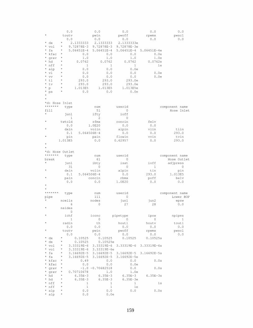
159
0.0 0.0 0.0 0.0 0.0 * toutv pwin pwoff rpwmx pwscl 0.0 0.0 0.0 0.0 0.0 * dx * 2.1333333 2.1333333 2.1333333e * vol * 9.72878E-3 9.72878E-3 9.72878E-3e * fa * 5.06451E-4 5.06451E-4 5.06451E-4 5.06451E-4e * kfac * 0.0 0.0 0.0 0.0e * grav * 1.0 1.0 1.0 1.0e * hd * 0.0762 0.0762 0.0762 0.0762e * nff * 1 1 1 1e * alp * 0.0 0.0 0.0e * vl * 0.0 0.0 0.0 0.0e * vv * 0.0 0.0 0.0 0.0e * tl * 293.0 293.0 293.0e * tv * 293.0 293.0 293.0e * p * 1.013E5 1.013E5 1.013E5e * pa * 0.0 0.0 0.0e * * *d: Hose Inlet ******* type num userid component name fill 51 0 Hose Inlet * jun1 ifty ioff 1 2 0 * twtold rfmx concin felv 0.0 1.0E20 0.0 0.0 * dxin volin alpin vlin tlin 0.1 5.064506E-4 0.0 0.0 293.0 * pin pain flowin vvin tvin 1.013E5 0.0 0.62957 0.0 293.0 * * *d: Hose Outlet ******* type num userid component name break 61 0 Hose Outlet * jun1 ibty isat ioff adjpress 31 0 0 1 0 * dxin volin alpin tin pin 0.1 5.064506E-4 0.0 293.0 1.013E5 * pain concin rbmx poff belv 0.0 0.0 1.0E20 0.0 0.0 * * ******* type num userid component name pipe 111 0 Lower BOP * ncells nodes jun1 jun2 epsw 6 0 27 28 0.0 * nsides 0 * ichf iconc pipetype ipow npipes 1 0 0 0 1 * radin th houtl houtv toutl 0.0 0.0 0.0 0.0 0.0 * toutv pwin pwoff rpwmx pwscl 0.0 0.0 0.0 0.0 0.0 * dx * 0.10525 0.10525 0.10525 0.10525s * dx * 0.10525 0.10525e * vol * 3.33319E-6 3.33319E-6 3.33319E-6 3.33319E-6s * vol * 3.33319E-6 3.33319E-6e * fa * 3.16692E-5 3.16692E-5 3.16692E-5 3.16692E-5s * fa * 3.16692E-5 3.16692E-5 3.16692E-5e * kfac * 0.49 0.0 0.0 0.0s * kfac * 0.0 0.0 0.0e * grav * -1.0 -0.70682518 0.0 0.0s * grav * 0.70710678 1.0 1.0e * hd * 6.35E-3 6.35E-3 6.35E-3 6.35E-3s * hd * 6.35E-3 6.35E-3 6.35E-3e * nff * 1 1 1 1s * nff * 1 1 1e * alp * 0.0 0.0 0.0 0.0s * alp * 0.0 0.0e

160
* vl * 0.0 0.0 0.0 0.0s * vl * 0.0 0.0 0.0e * vv * 0.0 0.0 0.0 0.0s * vv * 0.0 0.0 0.0e * tl * 378.0 378.0 378.0 378.0s * tl * 378.0 378.0e * tv * 378.149 378.149 378.149 378.149s * tv * 378.149 378.149e * p * 1.209E5 1.209E5 1.209E5 1.209E5s * p * 1.209E5 1.209E5e * pa * 0.0 0.0 0.0 0.0s * pa * 0.0 0.0e * * ******* type num userid component name pipe 112 0 Upper BOP * ncells nodes jun1 jun2 epsw 6 0 26 23 0.0 * nsides 0 * ichf iconc pipetype ipow npipes 1 0 0 0 1 * radin th houtl houtv toutl 0.0 0.0 0.0 0.0 0.0 * toutv pwin pwoff rpwmx pwscl 0.0 0.0 0.0 0.0 0.0 * dx * 0.0894667 0.0894667 0.0894667 0.0894667s * dx * 0.0894667 0.0894667e * vol * 2.83334E-6 2.83334E-6 2.83334E-6 2.83334E-6s * vol * 2.83334E-6 2.83334E-6e * fa * 3.16692E-5 3.16692E-5 3.16692E-5 3.16692E-5s * fa * 3.16692E-5 3.16692E-5 2.63022E-6e * kfac * 0.0 0.0 0.0 0.0s * kfac * 0.0 0.0 3.42e * grav * 1.0 1.0 1.0 0.0s * grav * 0.0 -1.0 -1.0e * hd * 6.35E-3 6.35E-3 6.35E-3 6.35E-3s * hd * 6.35E-3 6.35E-3 1.83E-3e * nff * 1 1 1 1s * nff * 1 1 1e * alp * 1.0 1.0 1.0 1.0s * alp * 1.0 1.0e * vl * 0.0 0.0 0.0 0.0s * vl * 0.0 0.0 0.0e * vv * 0.0 0.0 0.0 0.0s * vv * 0.0 0.0 0.0e * tl * 293.0 293.0 293.0 293.0s * tl * 293.0 293.0e * tv * 293.0 293.0 293.0 293.0s * tv * 293.0 293.0e * p * 1.013E5 1.013E5 1.013E5 1.013E5s * p * 1.013E5 1.013E5e * pa * 0.0 0.0 0.0 0.0s * pa * 0.0 0.0e * * *d: Nozzle * single junction ******* type num userid component name pipe 131 0 Nozzle * ncells nodes jun1 jun2 epsw 0 0 23 32 0.0 * ichf iconc pipetype ipow npipes 1 0 0 0 1 * radin th houtl houtv toutl 0.0 0.0 0.0 0.0 0.0 * toutv pwin pwoff rpwmx pwscl 0.0 0.0 0.0 0.0 0.0 * dx * f 0.0000e+00e * vol * f 0.0000e+00e * fa * f 2.63022E-6e

161
* kfac * f 3.42e * grav * f -1.0e * hd * f 1.83E-3e * nff * f 1e * alp * f 0.0000e+00e * vl * f 0.0e * vv * f 0.0e * tl * f 0.0000e+00e * tv * f 0.0000e+00e * p * f 0.0000e+00e * pa * f 0.0000e+00e * * ******* type num userid component name valve 151 0 unnamed * ncells nodes jun1 jun2 epsw 0 0 29 26 0.0 * ichf iconc ivty ivps nvtb2 1 0 1 1 0 * ivtr ivsv nvtb1 nvsv nvrf 0 30 6 0 0 * ivtrov ivtyov ivtrlo intlossoff nkopen 0 0 0 0 2 * rvmx rvov fminov fmaxov 100.0 0.0 0.0 1.0 * radin th houtl houtv toutl 0.0 0.0 0.0 0.0 0.0 * toutv avlve hvlve favlve xpos 0.0 3.166922E-5 6.35E-3 0.0 0.0 * dx * f 0.0000e+00e * vol * f 0.0000e+00e * fa * f 3.16692E-5e * kfac * f 0.0e * grav * f 1.0e * hd * f 6.35E-3e * nff * f 1e * alp * f 0.0000e+00e * vl * f 0.0e * vv * f 0.0e * tl * f 0.0000e+00e * tv * f 0.0000e+00e * p * f 0.0000e+00e * pa * f 0.0000e+00e * vtb1 * 0.0 0.0s * vtb1 * 1.0 0.0s * vtb1 * 2.0 0.0s * vtb1 * 3.0 0.0s * vtb1 * 4.0 0.0s * vtb1 * 5.0 1.0e * * ******************************************** * Starting Heat Structure Section of Model * ******************************************** * ******* type num userid component name htstr 101 1 unnamed * nzhstr ittc hscyl ichf 11 0 1 1 * nofuelrod plane liqlev iaxcnd pdrat 1 3 1 0 0.0 * nmwrx nfci nfcil hdri hdro 0 0 1 0.0 0.0 * nhot nodes fmon nzmax reflood 0 11 0 100 0 * dtxht(1) dtxht(2) dznht hgapo 0.0 0.0 1.0E-3 6300.0 * * idbcin * 2 2 2 2s * idbcin * 2 2 2 2s * idbcin * 2 2 2e

162
* idbcon * 5 5 5 5s * idbcon * 5 5 5 5s * idbcon * 5 5 5e * hcomon1 * 1 1 0 0e * hcomon1 * 1 2 0 0e * hcomon1 * 1 3 0 0e * hcomon1 * 1 4 0 0e * hcomon1 * 1 5 0 0e * hcomon1 * 1 6 0 0e * hcomon1 * 1 7 0 0e * hcomon1 * 1 8 0 0e * hcomon1 * 1 9 0 0e * hcomon1 * 1 10 0 0e * hcomon1 * 1 11 0 0e * tsurfo2 * 293.0e * tsurfo2 * 293.0e * tsurfo2 * 293.0e * tsurfo2 * 293.0e * tsurfo2 * 293.0e * tsurfo2 * 293.0e * tsurfo2 * 293.0e * tsurfo2 * 293.0e * tsurfo2 * 293.0e * tsurfo2 * 293.0e * tsurfo2 * 293.0e * dhtstrz * 0.58709091 0.58709091 0.58709091 0.58709091s * dhtstrz * 0.58709091 0.58709091 0.58709091 0.58709091s * dhtstrz * 0.58709091 0.58709091 0.58709091e * rdx * 1.0e * radrd * 0.038965 0.043325 0.0445 0.052045 0.056405s * radrd * 0.060765 0.065125 0.069485 0.073845 0.078205s * radrd * 0.082565e * matrd * 9 9 52 52 s * matrd * 52 52 52 52 s * matrd * 52 52 e * nfax * 1 1 1 1s * nfax * 1 1 1 1s * nfax * 1 1 1e * rftn * 373.0 373.0 373.0 373.0s * rftn * 363.0 353.0 343.0 333.0s * rftn * 323.0 313.0 303.0 373.0s * rftn * 373.0 373.0 373.0 363.0s * rftn * 353.0 343.0 333.0 323.0s * rftn * 313.0 303.0 373.0 373.0s * rftn * 373.0 373.0 363.0 353.0s * rftn * 343.0 333.0 323.0 313.0s * rftn * 303.0 373.0 373.0 373.0s * rftn * 373.0 363.0 353.0 343.0s * rftn * 333.0 323.0 313.0 303.0s * rftn * 373.0 373.0 373.0 373.0s * rftn * 363.0 353.0 343.0 333.0s * rftn * 323.0 313.0 303.0 373.0s * rftn * 373.0 373.0 373.0 363.0s * rftn * 353.0 343.0 333.0 323.0s * rftn * 313.0 303.0 373.0 373.0s * rftn * 373.0 373.0 363.0 353.0s * rftn * 343.0 333.0 323.0 313.0s * rftn * 303.0 373.0 373.0 373.0s * rftn * 373.0 363.0 353.0 343.0s * rftn * 333.0 323.0 313.0 303.0s * rftn * 373.0 373.0 373.0 373.0s * rftn * 363.0 353.0 343.0 333.0s * rftn * 323.0 313.0 303.0 373.0s * rftn * 373.0 373.0 373.0 363.0s * rftn * 353.0 343.0 333.0 323.0s * rftn * 313.0 303.0 373.0 373.0s * rftn * 373.0 373.0 363.0 353.0s * rftn * 343.0 333.0 323.0 313.0s * rftn * 303.0e * ******* type num userid component name

163
htstr 121 1 unnamed * nzhstr ittc hscyl ichf 6 0 1 1 * nofuelrod plane liqlev iaxcnd pdrat 1 3 1 0 0.0 * nmwrx nfci nfcil hdri hdro 0 0 1 0.0 0.0 * nhot nodes fmon nzmax reflood 0 6 0 100 0 * dtxht(1) dtxht(2) dznht hgapo 0.0 0.0 1.0E-3 6300.0 * * idbcin * 2 2 2 2s * idbcin * 2 2e * idbcon * 5 5 5 5s * idbcon * 5 5e * hcomon1 * 111 1 0 0e * hcomon1 * 111 2 0 0e * hcomon1 * 111 3 0 0e * hcomon1 * 111 4 0 0e * hcomon1 * 111 5 0 0e * hcomon1 * 111 6 0 0e * tsurfo2 * 293.0e * tsurfo2 * 293.0e * tsurfo2 * 293.0e * tsurfo2 * 293.0e * tsurfo2 * 293.0e * tsurfo2 * 293.0e * dhtstrz * 0.10525 0.10525 0.10525 0.10525s * dhtstrz * 0.10525 0.10525e * rdx * 1.0e * radrd * 3.175E-3 3.5052E-3 3.8354E-3 4.1656E-3 4.4958E-3s * radrd * 4.826E-3e * matrd * 50 50 50 50 s * matrd * 50 e * nfax * 1 1 1 1s * nfax * 1 1e * rftn * 378.0 378.0 378.0 378.0s * rftn * 378.0 378.0 378.0 378.0s * rftn * 378.0 378.0 378.0 378.0s * rftn * 378.0 378.0 378.0 378.0s * rftn * 378.0 378.0 378.0 378.0s * rftn * 378.0 378.0 378.0 378.0s * rftn * 378.0 378.0 378.0 378.0s * rftn * 378.0 378.0 378.0 378.0s * rftn * 378.0 378.0 378.0 378.0e * ******* type num userid component name htstr 122 1 unnamed * nzhstr ittc hscyl ichf 6 0 1 1 * nofuelrod plane liqlev iaxcnd pdrat 1 3 1 0 0.0 * nmwrx nfci nfcil hdri hdro 0 0 1 0.0 0.0 * nhot nodes fmon nzmax reflood 0 6 0 100 0 * dtxht(1) dtxht(2) dznht hgapo 0.0 0.0 1.0E-3 6300.0 * * idbcin * 2 2 2 2s * idbcin * 2 2e * idbcon * 5 5 5 5s * idbcon * 5 5e * hcomon1 * 112 1 0 0e * hcomon1 * 112 2 0 0e * hcomon1 * 112 3 0 0e * hcomon1 * 112 4 0 0e * hcomon1 * 112 5 0 0e * hcomon1 * 112 6 0 0e * tsurfo2 * 293.0e

164
* tsurfo2 * 293.0e * tsurfo2 * 293.0e * tsurfo2 * 293.0e * tsurfo2 * 293.0e * tsurfo2 * 293.0e * dhtstrz * 0.0894667 0.0894667 0.0894667 0.0894667s * dhtstrz * 0.0894667 0.0894667e * rdx * 1.0e * radrd * 3.175E-3 3.5052E-3 3.8354E-3 4.1656E-3 4.4958E-3s * radrd * 4.826E-3e * matrd * 50 50 50 50 s * matrd * 50 e * nfax * 1 1 1 1s * nfax * 1 1e * rftn * 373.0 373.0 373.0 373.0s * rftn * 373.0 373.0 373.0 373.0s * rftn * 373.0 373.0 373.0 373.0s * rftn * 373.0 373.0 373.0 373.0s * rftn * 373.0 373.0 373.0 373.0s * rftn * 373.0 373.0 373.0 373.0s * rftn * 373.0 373.0 373.0 373.0s * rftn * 373.0 373.0 373.0 373.0s * rftn * 373.0 373.0 373.0 373.0e * ******* type num userid component name htstr 132 1 unnamed * nzhstr ittc hscyl ichf 3 0 1 1 * nofuelrod plane liqlev iaxcnd pdrat 1 3 1 0 0.0 * nmwrx nfci nfcil hdri hdro 0 0 1 0.0 0.0 * nhot nodes fmon nzmax reflood 0 10 0 100 0 * dtxht(1) dtxht(2) dznht hgapo 0.0 0.0 1.0E-3 6300.0 * * idbcin * 2 2 2e * idbcon * 5 5 5e * hcomon1 * 31 1 0 0e * hcomon1 * 31 2 0 0e * hcomon1 * 31 3 0 0e * tsurfo2 * 293.0e * tsurfo2 * 293.0e * tsurfo2 * 293.0e * dhtstrz * 0.6196 0.6196 0.6196e * rdx * 1.0e * radrd * 0.0127 0.013205178 0.013710356 0.014215533 0.014720711s * radrd * 0.015225889 0.015731067 0.016236244 0.016741422 0.0172466e * matrd * 51 51 51 51 s * matrd * 51 51 51 51 s * matrd * 51 e * nfax * 1 1 1e * rftn * 293.0 293.0 293.0 293.0s * rftn * 293.0 293.0 293.0 293.0s * rftn * 293.0 293.0 293.0 293.0s * rftn * 293.0 293.0 293.0 293.0s * rftn * 293.0 293.0 293.0 293.0s * rftn * 293.0 293.0 293.0 293.0s * rftn * 293.0 293.0 293.0 293.0s * rftn * 293.0 293.0e * ******* type num userid component name htstr 141 1 unnamed * nzhstr ittc hscyl ichf 3 0 1 1 * nofuelrod plane liqlev iaxcnd pdrat 1 3 1 0 0.0 * nmwrx nfci nfcil hdri hdro 0 0 1 0.0 0.0 * nhot nodes fmon nzmax reflood

165
0 10 0 100 0 * dtxht(1) dtxht(2) dznht hgapo 0.0 0.0 1.0E-3 6300.0 * * idbcin * 2 2 2e * idbcon * 2 2 2e * hcomon1 * 21 1 0 0e * hcomon1 * 21 2 0 0e * hcomon1 * 21 3 0 0e * hcomon2 * 31 1 0 0e * hcomon2 * 31 2 0 0e * hcomon2 * 31 3 0 0e * dhtstrz * 0.6196 0.6196 0.6196e * rdx * 1.0e * radrd * 3.175E-3 3.35844E-3 3.54189E-3 3.72533E-3 3.90878E-3s * radrd * 4.09222E-3 4.27567E-3 4.45911E-3 4.64256E-3 4.826E-3e * matrd * 50 50 50 50 s * matrd * 50 50 50 50 s * matrd * 50 e * nfax * 1 1 1e * rftn * 293.0 293.0 293.0 293.0s * rftn * 293.0 293.0 293.0 293.0s * rftn * 293.0 293.0 293.0 293.0s * rftn * 293.0 293.0 293.0 293.0s * rftn * 293.0 293.0 293.0 293.0s * rftn * 293.0 293.0 293.0 293.0s * rftn * 293.0 293.0 293.0 293.0s * rftn * 293.0 293.0e * ******* type num userid component name htstr 161 1 unnamed * nzhstr ittc hscyl ichf 3 0 1 1 * nofuelrod plane liqlev iaxcnd pdrat 1 3 1 0 0.0 * nmwrx nfci nfcil hdri hdro 0 0 1 0.0 0.0 * nhot nodes fmon nzmax reflood 0 11 0 100 0 * dtxht(1) dtxht(2) dznht hgapo 0.0 0.0 1.0E-3 6300.0 * * idbcin * 2 2 2e * idbcon * 5 5 5e * hcomon1 * 11 1 0 0e * hcomon1 * 11 2 0 0e * hcomon1 * 11 3 0 0e * tsurfo2 * 293.0e * tsurfo2 * 293.0e * tsurfo2 * 293.0e * dhtstrz * 0.58709091 0.58709091 0.58709091e * rdx * 1.0e * radrd * 0.038965 0.043325 0.0445 0.052045 0.056405s * radrd * 0.060765 0.065125 0.069485 0.073845 0.078205s * radrd * 0.082565e * matrd * 9 9 52 52 s * matrd * 52 52 52 52 s * matrd * 52 52 e * nfax * 1 1 1e * rftn * 378.0 378.0 378.0 368.0s * rftn * 358.0 348.0 338.0 328.0s * rftn * 318.0 308.0 298.0 378.0s * rftn * 378.0 378.0 368.0 358.0s * rftn * 348.0 338.0 328.0 318.0s * rftn * 308.0 298.0 378.0 378.0s * rftn * 378.0 368.0 358.0 348.0s * rftn * 338.0 328.0 318.0 308.0s * rftn * 298.0e ******************************************** * Finished Heat Structure Section of Model * ********************************************
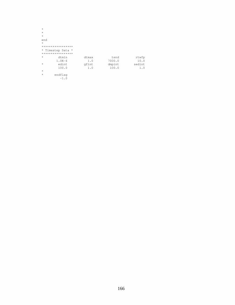
166
* * * end * ***************** * Timestep Data * ***************** * dtmin dtmax tend rtwfp 1.0E-6 1.0 7000.0 10.0 * edint gfint dmpint sedint 100.0 1.0 100.0 1.0 * * endflag -1.0
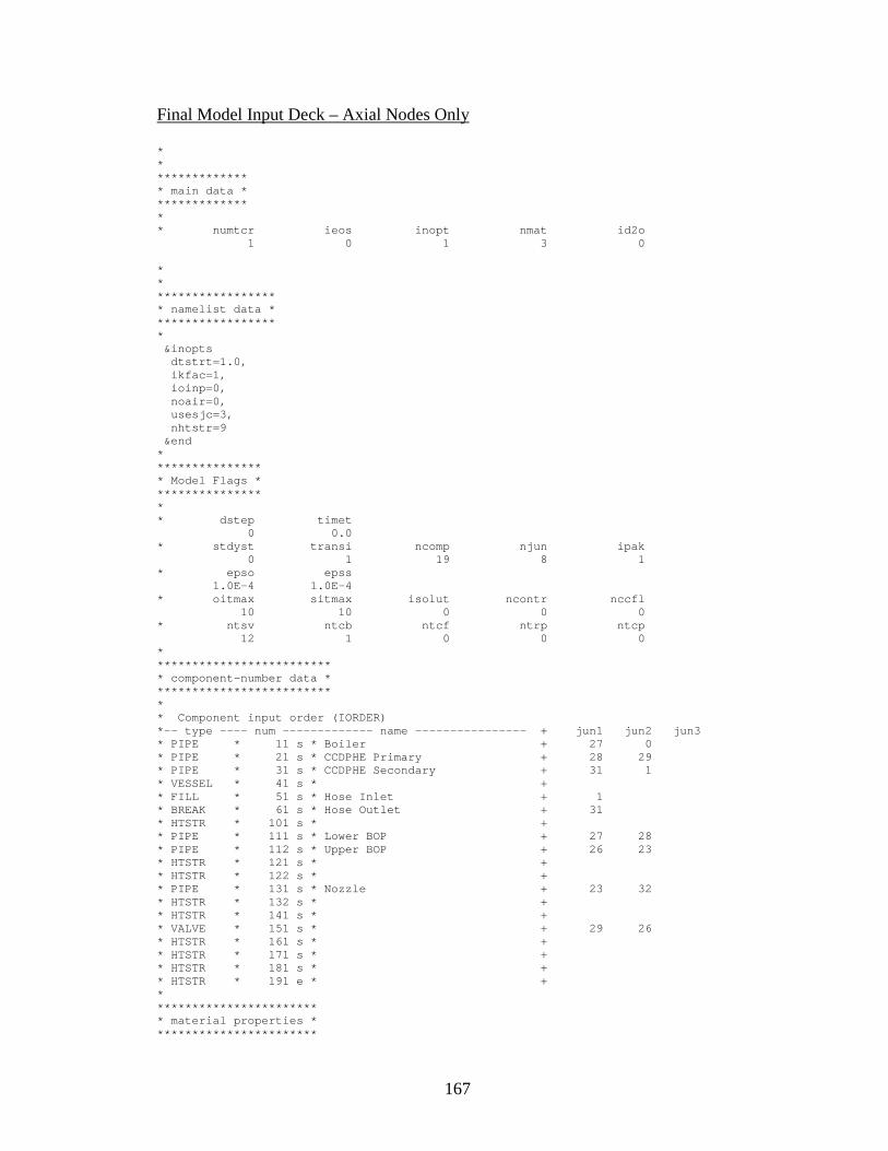
167
Final Model Input Deck – Axial Nodes Only
* * ************* * main data * ************* * * numtcr ieos inopt nmat id2o 1 0 1 3 0 * * ***************** * namelist data * ***************** * &inopts dtstrt=1.0, ikfac=1, ioinp=0, noair=0, usesjc=3, nhtstr=9 &end * *************** * Model Flags * *************** * * dstep timet 0 0.0 * stdyst transi ncomp njun ipak 0 1 19 8 1 * epso epss 1.0E-4 1.0E-4 * oitmax sitmax isolut ncontr nccfl 10 10 0 0 0 * ntsv ntcb ntcf ntrp ntcp 12 1 0 0 0 * ************************* * component-number data * ************************* * * Component input order (IORDER) *-- type ---- num ------------- name ---------------- + jun1 jun2 jun3 * PIPE * 11 s * Boiler + 27 0 * PIPE * 21 s * CCDPHE Primary + 28 29 * PIPE * 31 s * CCDPHE Secondary + 31 1 * VESSEL * 41 s * + * FILL * 51 s * Hose Inlet + 1 * BREAK * 61 s * Hose Outlet + 31 * HTSTR * 101 s * + * PIPE * 111 s * Lower BOP + 27 28 * PIPE * 112 s * Upper BOP + 26 23 * HTSTR * 121 s * + * HTSTR * 122 s * + * PIPE * 131 s * Nozzle + 23 32 * HTSTR * 132 s * + * HTSTR * 141 s * + * VALVE * 151 s * + 29 26 * HTSTR * 161 s * + * HTSTR * 171 s * + * HTSTR * 181 s * + * HTSTR * 191 e * + * *********************** * material properties * ***********************

168
* * matb* 50 51 52 e * ptbln* 1 1 1 e * User Defined Material : 50 * *n: Copper Alloy * *d: Copper Alloy * prptb temp rho cp cond emis * prptb* 293.0 8940.6 385.0 394.0 0.0 e * * User Defined Material : 51 * *n: PVC * * prptb temp rho cp cond emis * prptb* 293.0 1390.0 900.0 0.16 0.0 e * * User Defined Material : 52 * *n: Insulation * * prptb temp rho cp cond emis * prptb* 293.0 48.05539 670.0 0.033172414 0.0 e * * * ************************************************** * Starting Signal Variable Section of Model * ************************************************** *n: Boiler Pressure * * idsv isvn ilcn icn1 icn2 1 21 11 3 0 *n: BC21 * * idsv isvn ilcn icn1 icn2 13 23 11 3 0 *n: BC11 * * idsv isvn ilcn icn1 icn2 14 23 11 2 0 *n: BC01 * * idsv isvn ilcn icn1 icn2 15 23 11 1 0 *n: Primary Inlet * * idsv isvn ilcn icn1 icn2 16 23 51 1 0 *n: Primary Outlet * * idsv isvn ilcn icn1 icn2 17 23 61 1 0 *n: Condenser Pressure * * idsv isvn ilcn icn1 icn2 24 21 41 1011 0 *n: Boiler Inventory * *d: FlashLevel * idsv isvn ilcn icn1 icn2 25 124 11 0 0 *n: Boiler Initial Inventory * *d: FlashIntLevel * idsv isvn ilcn icn1 icn2 26 125 11 0 0 *n: Condenser Initial Inventory * *d: CondeIntLevel

169
* idsv isvn ilcn icn1 icn2 27 125 0 0 0 *n: Condenser Inventory * *d: CondeLevel * idsv isvn ilcn icn1 icn2 28 124 0 0 0 *n: Timer * * idsv isvn ilcn icn1 icn2 30 0 0 0 0 ************************************************** * Finished Signal Variable Section of Model * ************************************************** * * * * ********************************************* * Starting Control System Section of Model * ********************************************* * ****** Control Blocks ****** *n: PressDif * *d: PressDif * idcb icbn icb1 icb2 icb3 -1 44 1 24 0 * cbgain cbxmin cbmax cbcon1 cbcon2 1.0 -1.0E20 1.0E20 0.0 0.0 * ********************************************* * Finished Control System Section of Model * ********************************************* * * * * ******* type num userid component name pipe 11 0 Boiler * ncells nodes jun1 jun2 epsw 3 0 27 0 0.0 * nsides 0 * ichf iconc pipetype ipow npipes 1 0 0 0 1 * radin th houtl houtv toutl 0.0 0.0 0.0 0.0 0.0 * toutv pwin pwoff rpwmx pwscl 0.0 0.0 0.0 0.0 0.0 * dx * 2.1333333 2.1333333 2.1333333e * vol * 9.72878E-3 9.72878E-3 9.72878E-3e * fa * 3.16692E-5 4.56037E-3 4.56037E-3 4.56037E-3e * kfac * 0.49 0.0 0.0 0.0e * grav * 1.0 1.0 1.0 1.0e * hd * 6.35E-3 0.0762 0.0762 0.0762e * nff * 1 1 1 1e * alp * 0.0 0.0 0.0e * vl * 0.0 0.0 0.0 0.0e * vv * 0.0 0.0 0.0 0.0e * tl * 378.149 378.149 378.149e * tv * 378.149 378.149 378.149e * p * 1.209E5 1.209E5 1.209E5e * pa * 0.0 0.0 0.0e * * ******* type num userid component name pipe 21 0 CCDPHE Primary * ncells nodes jun1 jun2 epsw 3 0 28 29 0.0 * nsides

170
0 * ichf iconc pipetype ipow npipes 1 0 0 0 1 * radin th houtl houtv toutl 0.0 0.0 0.0 0.0 0.0 * toutv pwin pwoff rpwmx pwscl 0.0 0.0 0.0 0.0 0.0 * dx * 2.1333333 2.1333333 2.1333333e * vol * 6.7561E-5 6.7561E-5 6.7561E-5e * fa * 3.16692E-5 3.16692E-5 3.16692E-5 3.16692E-5e * kfac * 0.0 0.0 0.0 0.0e * grav * 1.0 1.0 1.0 1.0e * hd * 6.35E-3 6.35E-3 6.35E-3 6.35E-3e * nff * 1 1 1 1e * alp * 1.0 1.0 1.0e * vl * 0.0 0.0 0.0 0.0e * vv * 0.0 0.0 0.0 0.0e * tl * 293.0 293.0 293.0e * tv * 293.0 293.0 293.0e * p * 1.209E5 1.209E5 1.209E5e * pa * 101300.0 101300.0 101300.0e * * ******* type num userid component name pipe 31 0 CCDPHE Secondary * ncells nodes jun1 jun2 epsw 3 0 31 1 0.0 * nsides 0 * ichf iconc pipetype ipow npipes 1 0 0 0 1 * radin th houtl houtv toutl 0.0 0.0 0.0 0.0 0.0 * toutv pwin pwoff rpwmx pwscl 0.0 0.0 0.0 0.0 0.0 * dx * 2.1333333 2.1333333 2.1333333e * vol * 9.72878E-3 9.72878E-3 9.72878E-3e * fa * 5.06451E-4 5.06451E-4 5.06451E-4 5.06451E-4e * kfac * 0.0 0.0 0.0 0.0e * grav * 1.0 1.0 1.0 1.0e * hd * 0.0762 0.0762 0.0762 0.0762e * nff * 1 1 1 1e * alp * 0.0 0.0 0.0e * vl * 0.0 0.0 0.0 0.0e * vv * 0.0 0.0 0.0 0.0e * tl * 293.0 293.0 293.0e * tv * 293.0 293.0 293.0e * p * 1.013E5 1.013E5 1.013E5e * pa * 0.0 0.0 0.0e * * ******* type num userid component name vessel 41 0 unnamed * nasx nrsx ntsx ncsr ivssbf 11 1 1 1 0 * idcu idcl idcr icru icrl 0 0 0 0 0 * icrr ilcsp iucsp iuhp iconc 0 0 0 0 0 * igeom nvent nvvtb nsgrid vesstype 0 0 0 0 0 * shelv epsw 0.0 0.0 * z * 0.58181818 1.1636364 1.7454545 2.3272727s * z * 2.9090909 3.4909091 4.0727273 4.6545455s * z * 5.2363636 5.8181818 6.4e * r * 0.0381e * t * 360.0e * lisrl lisrc lisrf ljuns zfrac 11 1 2 32 * level 1

171
* * cfzlyt * 0.0e * cfzlz * 0.0e * cfzlxr * 0.0e * cfzvyt * 0.0e * cfzvz * 0.0e * cfzvxr * 0.0e * frvol * 1.0e * frfayt * 1.0e * frfaz * 1.0e * frfaxr * 0.5e * hdyt * 0.0381e * hdz * 4.56E-3e * hdxr * 4.56E-3e * alpn * 0.0e * vvnyt * 0.0e * vvnz * 0.0e * vvnxr * 0.0e * vlnyt * 0.0e * vlnz * 0.0e * vlnxr * 0.0e * tvn * 373.117e * tln * 373.117e * pn * 1.013E5e * pan * 0.0e * level 2 * * cfzlyt * 0.0e * cfzlz * 0.0e * cfzlxr * 0.0e * cfzvyt * 0.0e * cfzvz * 0.0e * cfzvxr * 0.0e * frvol * 1.0e * frfayt * 1.0e * frfaz * 1.0e * frfaxr * 0.5e * hdyt * 0.0381e * hdz * 4.56E-3e * hdxr * 4.56E-3e * alpn * 0.65e * vvnyt * 0.0e * vvnz * 0.0e * vvnxr * 0.0e * vlnyt * 0.0e * vlnz * 0.0e * vlnxr * 0.0e * tvn * 373.117e * tln * 373.117e * pn * 1.013E5e * pan * 0.0e * level 3 * * cfzlyt * 0.0e * cfzlz * 0.0e * cfzlxr * 0.0e * cfzvyt * 0.0e * cfzvz * 0.0e * cfzvxr * 0.0e * frvol * 1.0e * frfayt * 1.0e * frfaz * 1.0e * frfaxr * 0.5e * hdyt * 0.0381e * hdz * 4.56E-3e * hdxr * 4.56E-3e * alpn * 1.0e * vvnyt * 0.0e * vvnz * 0.0e * vvnxr * 0.0e * vlnyt * 0.0e

172
* vlnz * 0.0e * vlnxr * 0.0e * tvn * 373.117e * tln * 373.117e * pn * 1.013E5e * pan * 0.0e * level 4 * * cfzlyt * 0.0e * cfzlz * 0.0e * cfzlxr * 0.0e * cfzvyt * 0.0e * cfzvz * 0.0e * cfzvxr * 0.0e * frvol * 1.0e * frfayt * 1.0e * frfaz * 1.0e * frfaxr * 0.5e * hdyt * 0.0381e * hdz * 4.56E-3e * hdxr * 4.56E-3e * alpn * 1.0e * vvnyt * 0.0e * vvnz * 0.0e * vvnxr * 0.0e * vlnyt * 0.0e * vlnz * 0.0e * vlnxr * 0.0e * tvn * 373.117e * tln * 373.117e * pn * 1.013E5e * pan * 0.0e * level 5 * * cfzlyt * 0.0e * cfzlz * 0.0e * cfzlxr * 0.0e * cfzvyt * 0.0e * cfzvz * 0.0e * cfzvxr * 0.0e * frvol * 1.0e * frfayt * 1.0e * frfaz * 1.0e * frfaxr * 0.5e * hdyt * 0.0381e * hdz * 4.56E-3e * hdxr * 4.56E-3e * alpn * 1.0e * vvnyt * 0.0e * vvnz * 0.0e * vvnxr * 0.0e * vlnyt * 0.0e * vlnz * 0.0e * vlnxr * 0.0e * tvn * 373.117e * tln * 373.117e * pn * 1.013E5e * pan * 0.0e * level 6 * * cfzlyt * 0.0e * cfzlz * 0.0e * cfzlxr * 0.0e * cfzvyt * 0.0e * cfzvz * 0.0e * cfzvxr * 0.0e * frvol * 1.0e * frfayt * 1.0e * frfaz * 1.0e * frfaxr * 0.5e * hdyt * 0.0381e
173
* hdz * 4.56E-3e * hdxr * 4.56E-3e * alpn * 1.0e * vvnyt * 0.0e * vvnz * 0.0e * vvnxr * 0.0e * vlnyt * 0.0e * vlnz * 0.0e * vlnxr * 0.0e * tvn * 373.117e * tln * 373.117e * pn * 1.013E5e * pan * 0.0e * level 7 * * cfzlyt * 0.0e * cfzlz * 0.0e * cfzlxr * 0.0e * cfzvyt * 0.0e * cfzvz * 0.0e * cfzvxr * 0.0e * frvol * 1.0e * frfayt * 1.0e * frfaz * 1.0e * frfaxr * 0.5e * hdyt * 0.0381e * hdz * 4.56E-3e * hdxr * 4.56E-3e * alpn * 1.0e * vvnyt * 0.0e * vvnz * 0.0e * vvnxr * 0.0e * vlnyt * 0.0e * vlnz * 0.0e * vlnxr * 0.0e * tvn * 373.117e * tln * 373.117e * pn * 1.013E5e * pan * 0.0e * level 8 * * cfzlyt * 0.0e * cfzlz * 0.0e * cfzlxr * 0.0e * cfzvyt * 0.0e * cfzvz * 0.0e * cfzvxr * 0.0e * frvol * 1.0e * frfayt * 1.0e * frfaz * 1.0e * frfaxr * 0.5e * hdyt * 0.0381e * hdz * 4.56E-3e * hdxr * 4.56E-3e * alpn * 1.0e * vvnyt * 0.0e * vvnz * 0.0e * vvnxr * 0.0e * vlnyt * 0.0e * vlnz * 0.0e * vlnxr * 0.0e * tvn * 373.117e * tln * 373.117e * pn * 1.013E5e * pan * 0.0e * level 9 * * cfzlyt * 0.0e * cfzlz * 0.0e * cfzlxr * 0.0e * cfzvyt * 0.0e

174
* cfzvz * 0.0e * cfzvxr * 0.0e * frvol * 1.0e * frfayt * 1.0e * frfaz * 1.0e * frfaxr * 0.5e * hdyt * 0.0381e * hdz * 4.56E-3e * hdxr * 4.56E-3e * alpn * 1.0e * vvnyt * 0.0e * vvnz * 0.0e * vvnxr * 0.0e * vlnyt * 0.0e * vlnz * 0.0e * vlnxr * 0.0e * tvn * 373.117e * tln * 373.117e * pn * 1.013E5e * pan * 0.0e * level 10 * * cfzlyt * 0.0e * cfzlz * 0.0e * cfzlxr * 0.0e * cfzvyt * 0.0e * cfzvz * 0.0e * cfzvxr * 0.0e * frvol * 1.0e * frfayt * 1.0e * frfaz * 1.0e * frfaxr * 0.5e * hdyt * 0.0381e * hdz * 4.56E-3e * hdxr * 4.56E-3e * alpn * 1.0e * vvnyt * 0.0e * vvnz * 0.0e * vvnxr * 0.0e * vlnyt * 0.0e * vlnz * 0.0e * vlnxr * 0.0e * tvn * 373.117e * tln * 373.117e * pn * 1.013E5e * pan * 0.0e * level 11 * * cfzlyt * 0.0e * cfzlz * -1.0E-20e * cfzlxr * 0.0e * cfzvyt * 0.0e * cfzvz * 0.0e * cfzvxr * 0.0e * frvol * 1.0e * frfayt * 1.0e * frfaz * 1.0e * frfaxr * 0.5e * hdyt * 0.0381e * hdz * -4.56E-3e * hdxr * 4.56E-3e * alpn * 1.0e * vvnyt * 0.0e * vvnz * 0.0e * vvnxr * 0.0e * vlnyt * 0.0e * vlnz * 0.0e * vlnxr * 0.0e * tvn * 373.117e * tln * 373.117e * pn * 1.013E5e

175
* pan * 0.0e * * *d: Hose Inlet ******* type num userid component name fill 51 0 Hose Inlet * jun1 ifty ioff 1 2 0 * twtold rfmx concin felv 0.0 1.0E20 0.0 0.0 * dxin volin alpin vlin tlin 0.1 5.064506E-4 0.0 0.0 293.0 * pin pain flowin vvin tvin 1.013E5 0.0 0.62957 0.0 293.0 * * *d: Hose Outlet ******* type num userid component name break 61 0 Hose Outlet * jun1 ibty isat ioff adjpress 31 0 0 1 0 * dxin volin alpin tin pin 0.1 5.064506E-4 0.0 293.0 1.013E5 * pain concin rbmx poff belv 0.0 0.0 1.0E20 0.0 0.0 * * ******* type num userid component name pipe 111 0 Lower BOP * ncells nodes jun1 jun2 epsw 6 0 27 28 0.0 * nsides 0 * ichf iconc pipetype ipow npipes 1 0 0 0 1 * radin th houtl houtv toutl 0.0 0.0 0.0 0.0 0.0 * toutv pwin pwoff rpwmx pwscl 0.0 0.0 0.0 0.0 0.0 * dx * 0.10525 0.10525 0.10525 0.10525s * dx * 0.10525 0.10525e * vol * 3.33319E-6 3.33319E-6 3.33319E-6 3.33319E-6s * vol * 3.33319E-6 3.33319E-6e * fa * 3.16692E-5 3.16692E-5 3.16692E-5 3.16692E-5s * fa * 3.16692E-5 3.16692E-5 3.16692E-5e * kfac * 0.49 0.0 0.0 0.0s * kfac * 0.0 0.0 0.0e * grav * -1.0 -0.70682518 0.0 0.0s * grav * 0.70710678 1.0 1.0e * hd * 6.35E-3 6.35E-3 6.35E-3 6.35E-3s * hd * 6.35E-3 6.35E-3 6.35E-3e * nff * 1 1 1 1s * nff * 1 1 1e * alp * 0.0 0.0 0.0 0.0s * alp * 0.0 0.0e * vl * 0.0 0.0 0.0 0.0s * vl * 0.0 0.0 0.0e * vv * 0.0 0.0 0.0 0.0s * vv * 0.0 0.0 0.0e * tl * 378.0 378.0 378.0 378.0s * tl * 378.0 378.0e * tv * 378.149 378.149 378.149 378.149s * tv * 378.149 378.149e * p * 1.209E5 1.209E5 1.209E5 1.209E5s * p * 1.209E5 1.209E5e * pa * 0.0 0.0 0.0 0.0s * pa * 0.0 0.0e * * ******* type num userid component name pipe 112 0 Upper BOP

176
* ncells nodes jun1 jun2 epsw 6 0 26 23 0.0 * nsides 0 * ichf iconc pipetype ipow npipes 1 0 0 0 1 * radin th houtl houtv toutl 0.0 0.0 0.0 0.0 0.0 * toutv pwin pwoff rpwmx pwscl 0.0 0.0 0.0 0.0 0.0 * dx * 0.0894667 0.0894667 0.0894667 0.0894667s * dx * 0.0894667 0.0894667e * vol * 2.83334E-6 2.83334E-6 2.83334E-6 2.83334E-6s * vol * 2.83334E-6 2.83334E-6e * fa * 3.16692E-5 3.16692E-5 3.16692E-5 3.16692E-5s * fa * 3.16692E-5 3.16692E-5 2.63022E-6e * kfac * 0.0 0.0 0.0 0.0s * kfac * 0.0 0.0 3.42e * grav * 1.0 1.0 1.0 0.0s * grav * 0.0 -1.0 -1.0e * hd * 6.35E-3 6.35E-3 6.35E-3 6.35E-3s * hd * 6.35E-3 6.35E-3 1.83E-3e * nff * 1 1 1 1s * nff * 1 1 1e * alp * 1.0 1.0 1.0 1.0s * alp * 1.0 1.0e * vl * 0.0 0.0 0.0 0.0s * vl * 0.0 0.0 0.0e * vv * 0.0 0.0 0.0 0.0s * vv * 0.0 0.0 0.0e * tl * 293.0 293.0 293.0 293.0s * tl * 293.0 293.0e * tv * 293.0 293.0 293.0 293.0s * tv * 293.0 293.0e * p * 1.013E5 1.013E5 1.013E5 1.013E5s * p * 1.013E5 1.013E5e * pa * 0.0 0.0 0.0 0.0s * pa * 0.0 0.0e * * *d: Nozzle * single junction ******* type num userid component name pipe 131 0 Nozzle * ncells nodes jun1 jun2 epsw 0 0 23 32 0.0 * ichf iconc pipetype ipow npipes 1 0 0 0 1 * radin th houtl houtv toutl 0.0 0.0 0.0 0.0 0.0 * toutv pwin pwoff rpwmx pwscl 0.0 0.0 0.0 0.0 0.0 * dx * f 0.0000e+00e * vol * f 0.0000e+00e * fa * f 2.63022E-6e * kfac * f 3.42e * grav * f -1.0e * hd * f 1.83E-3e * nff * f 1e * alp * f 0.0000e+00e * vl * f 0.0e * vv * f 0.0e * tl * f 0.0000e+00e * tv * f 0.0000e+00e * p * f 0.0000e+00e * pa * f 0.0000e+00e * * ******* type num userid component name valve 151 0 unnamed * ncells nodes jun1 jun2 epsw

177
0 0 29 26 0.0 * ichf iconc ivty ivps nvtb2 1 0 1 1 0 * ivtr ivsv nvtb1 nvsv nvrf 0 30 6 0 0 * ivtrov ivtyov ivtrlo intlossoff nkopen 0 0 0 0 2 * rvmx rvov fminov fmaxov 100.0 0.0 0.0 1.0 * radin th houtl houtv toutl 0.0 0.0 0.0 0.0 0.0 * toutv avlve hvlve favlve xpos 0.0 3.166922E-5 6.35E-3 0.0 0.0 * dx * f 0.0000e+00e * vol * f 0.0000e+00e * fa * f 3.16692E-5e * kfac * f 0.0e * grav * f 1.0e * hd * f 6.35E-3e * nff * f 1e * alp * f 0.0000e+00e * vl * f 0.0e * vv * f 0.0e * tl * f 0.0000e+00e * tv * f 0.0000e+00e * p * f 0.0000e+00e * pa * f 0.0000e+00e * vtb1 * 0.0 0.0s * vtb1 * 1.0 0.0s * vtb1 * 2.0 0.0s * vtb1 * 3.0 0.0s * vtb1 * 4.0 0.0s * vtb1 * 5.0 1.0e * * ******************************************** * Starting Heat Structure Section of Model * ******************************************** * ******* type num userid component name htstr 101 1 unnamed * nzhstr ittc hscyl ichf 11 0 1 1 * nofuelrod plane liqlev iaxcnd pdrat 1 3 1 0 0.0 * nmwrx nfci nfcil hdri hdro 0 0 1 0.0 0.0 * nhot nodes fmon nzmax reflood 0 11 0 210 0 * dtxht(1) dtxht(2) dznht hgapo 0.0 0.0 1.0E-3 6300.0 * * idbcin * 2 2 2 2s * idbcin * 2 2 2 2s * idbcin * 2 2 2e * idbcon * 5 5 5 5s * idbcon * 5 5 5 5s * idbcon * 5 5 5e * hcomon1 * 41 1 1 1e * hcomon1 * 41 1 1 2e * hcomon1 * 41 1 1 3e * hcomon1 * 41 1 1 4e * hcomon1 * 41 1 1 5e * hcomon1 * 41 1 1 6e * hcomon1 * 41 1 1 7e * hcomon1 * 41 1 1 8e * hcomon1 * 41 1 1 9e * hcomon1 * 41 1 1 10e * hcomon1 * 41 1 1 11e * tsurfo2 * 293.0e * tsurfo2 * 293.0e

178
* tsurfo2 * 293.0e * tsurfo2 * 293.0e * tsurfo2 * 293.0e * tsurfo2 * 293.0e * tsurfo2 * 293.0e * tsurfo2 * 293.0e * tsurfo2 * 293.0e * tsurfo2 * 293.0e * tsurfo2 * 293.0e * dhtstrz * 0.39315152 0.19393939 0.39315152 0.19393939s * dhtstrz * 0.39315152 0.19393939 0.39315152 0.19393939s * dhtstrz * 0.39315152 0.19393939 0.39315152e * rdx * 0.5e * radrd * 0.038965 0.039222676 0.039265404 0.052045 0.056405s * radrd * 0.060765 0.065125 0.069485 0.073845 0.078205s * radrd * 0.082565e * matrd * 9 9 52 52 s * matrd * 52 52 52 52 s * matrd * 52 52 e * nfax * 1 1 1 1s * nfax * 1 1 1 1s * nfax * 1 1 1e * rftn * 373.0 373.0 373.0 373.0s * rftn * 363.0 353.0 343.0 333.0s * rftn * 323.0 313.0 303.0 373.0s * rftn * 373.0 373.0 373.0 363.0s * rftn * 353.0 343.0 333.0 323.0s * rftn * 313.0 303.0 373.0 373.0s * rftn * 373.0 373.0 363.0 353.0s * rftn * 343.0 333.0 323.0 313.0s * rftn * 303.0 373.0 373.0 373.0s * rftn * 373.0 363.0 353.0 343.0s * rftn * 333.0 323.0 313.0 303.0s * rftn * 373.0 373.0 373.0 373.0s * rftn * 363.0 353.0 343.0 333.0s * rftn * 323.0 313.0 303.0 373.0s * rftn * 373.0 373.0 373.0 363.0s * rftn * 353.0 343.0 333.0 323.0s * rftn * 313.0 303.0 373.0 373.0s * rftn * 373.0 373.0 363.0 353.0s * rftn * 343.0 333.0 323.0 313.0s * rftn * 303.0 373.0 373.0 373.0s * rftn * 373.0 363.0 353.0 343.0s * rftn * 333.0 323.0 313.0 303.0s * rftn * 373.0 373.0 373.0 373.0s * rftn * 363.0 353.0 343.0 333.0s * rftn * 323.0 313.0 303.0 373.0s * rftn * 373.0 373.0 373.0 363.0s * rftn * 353.0 343.0 333.0 323.0s * rftn * 313.0 303.0 373.0 373.0s * rftn * 373.0 373.0 363.0 353.0s * rftn * 343.0 333.0 323.0 313.0s * rftn * 303.0e * ******* type num userid component name htstr 121 1 unnamed * nzhstr ittc hscyl ichf 6 0 1 1 * nofuelrod plane liqlev iaxcnd pdrat 1 3 1 0 0.0 * nmwrx nfci nfcil hdri hdro 0 0 1 0.0 0.0 * nhot nodes fmon nzmax reflood 0 6 0 100 0 * dtxht(1) dtxht(2) dznht hgapo 0.0 0.0 1.0E-3 6300.0 * * idbcin * 2 2 2 2s * idbcin * 2 2e * idbcon * 5 5 5 5s * idbcon * 5 5e

179
* hcomon1 * 111 1 0 0e * hcomon1 * 111 2 0 0e * hcomon1 * 111 3 0 0e * hcomon1 * 111 4 0 0e * hcomon1 * 111 5 0 0e * hcomon1 * 111 6 0 0e * tsurfo2 * 293.0e * tsurfo2 * 293.0e * tsurfo2 * 293.0e * tsurfo2 * 293.0e * tsurfo2 * 293.0e * tsurfo2 * 293.0e * dhtstrz * 0.10525 0.10525 0.10525 0.10525s * dhtstrz * 0.10525 0.10525e * rdx * 1.0e * radrd * 3.175E-3 3.5052E-3 3.8354E-3 4.1656E-3 4.4958E-3s * radrd * 4.826E-3e * matrd * 50 50 50 50 s * matrd * 50 e * nfax * 1 1 1 1s * nfax * 1 1e * rftn * 378.0 378.0 378.0 378.0s * rftn * 378.0 378.0 378.0 378.0s * rftn * 378.0 378.0 378.0 378.0s * rftn * 378.0 378.0 378.0 378.0s * rftn * 378.0 378.0 378.0 378.0s * rftn * 378.0 378.0 378.0 378.0s * rftn * 378.0 378.0 378.0 378.0s * rftn * 378.0 378.0 378.0 378.0s * rftn * 378.0 378.0 378.0 378.0e * ******* type num userid component name htstr 122 1 unnamed * nzhstr ittc hscyl ichf 6 0 1 1 * nofuelrod plane liqlev iaxcnd pdrat 1 3 1 0 0.0 * nmwrx nfci nfcil hdri hdro 0 0 1 0.0 0.0 * nhot nodes fmon nzmax reflood 0 6 0 100 0 * dtxht(1) dtxht(2) dznht hgapo 0.0 0.0 1.0E-3 6300.0 * * idbcin * 2 2 2 2s * idbcin * 2 2e * idbcon * 5 5 5 5s * idbcon * 5 5e * hcomon1 * 112 1 0 0e * hcomon1 * 112 2 0 0e * hcomon1 * 112 3 0 0e * hcomon1 * 112 4 0 0e * hcomon1 * 112 5 0 0e * hcomon1 * 112 6 0 0e * tsurfo2 * 293.0e * tsurfo2 * 293.0e * tsurfo2 * 293.0e * tsurfo2 * 293.0e * tsurfo2 * 293.0e * tsurfo2 * 293.0e * dhtstrz * 0.0894667 0.0894667 0.0894667 0.0894667s * dhtstrz * 0.0894667 0.0894667e * rdx * 1.0e * radrd * 3.175E-3 3.5052E-3 3.8354E-3 4.1656E-3 4.4958E-3s * radrd * 4.826E-3e * matrd * 50 50 50 50 s * matrd * 50 e * nfax * 1 1 1 1s * nfax * 1 1e * rftn * 373.0 373.0 373.0 373.0s * rftn * 373.0 373.0 373.0 373.0s

180
* rftn * 373.0 373.0 373.0 373.0s * rftn * 373.0 373.0 373.0 373.0s * rftn * 373.0 373.0 373.0 373.0s * rftn * 373.0 373.0 373.0 373.0s * rftn * 373.0 373.0 373.0 373.0s * rftn * 373.0 373.0 373.0 373.0s * rftn * 373.0 373.0 373.0 373.0e * ******* type num userid component name htstr 132 1 unnamed * nzhstr ittc hscyl ichf 3 0 1 1 * nofuelrod plane liqlev iaxcnd pdrat 1 3 1 0 0.0 * nmwrx nfci nfcil hdri hdro 0 0 1 0.0 0.0 * nhot nodes fmon nzmax reflood 0 10 0 100 0 * dtxht(1) dtxht(2) dznht hgapo 0.0 0.0 1.0E-3 6300.0 * * idbcin * 2 2 2e * idbcon * 5 5 5e * hcomon1 * 31 1 0 0e * hcomon1 * 31 2 0 0e * hcomon1 * 31 3 0 0e * tsurfo2 * 293.0e * tsurfo2 * 293.0e * tsurfo2 * 293.0e * dhtstrz * 0.6196 0.6196 0.6196e * rdx * 1.0e * radrd * 0.0127 0.013205178 0.013710356 0.014215533 0.014720711s * radrd * 0.015225889 0.015731067 0.016236244 0.016741422 0.0172466e * matrd * 51 51 51 51 s * matrd * 51 51 51 51 s * matrd * 51 e * nfax * 1 1 1e * rftn * 293.0 293.0 293.0 293.0s * rftn * 293.0 293.0 293.0 293.0s * rftn * 293.0 293.0 293.0 293.0s * rftn * 293.0 293.0 293.0 293.0s * rftn * 293.0 293.0 293.0 293.0s * rftn * 293.0 293.0 293.0 293.0s * rftn * 293.0 293.0 293.0 293.0s * rftn * 293.0 293.0e * ******* type num userid component name htstr 141 1 unnamed * nzhstr ittc hscyl ichf 3 0 1 1 * nofuelrod plane liqlev iaxcnd pdrat 1 3 1 0 0.0 * nmwrx nfci nfcil hdri hdro 0 0 1 0.0 0.0 * nhot nodes fmon nzmax reflood 0 10 0 100 0 * dtxht(1) dtxht(2) dznht hgapo 0.0 0.0 1.0E-3 6300.0 * * idbcin * 2 2 2e * idbcon * 2 2 2e * hcomon1 * 21 1 0 0e * hcomon1 * 21 2 0 0e * hcomon1 * 21 3 0 0e * hcomon2 * 31 1 0 0e * hcomon2 * 31 2 0 0e * hcomon2 * 31 3 0 0e * dhtstrz * 0.6196 0.6196 0.6196e * rdx * 1.0e * radrd * 3.175E-3 3.35844E-3 3.54189E-3 3.72533E-3 3.90878E-3s * radrd * 4.09222E-3 4.27567E-3 4.45911E-3 4.64256E-3 4.826E-3e
181
* matrd * 50 50 50 50 s * matrd * 50 50 50 50 s * matrd * 50 e * nfax * 1 1 1e * rftn * 293.0 293.0 293.0 293.0s * rftn * 293.0 293.0 293.0 293.0s * rftn * 293.0 293.0 293.0 293.0s * rftn * 293.0 293.0 293.0 293.0s * rftn * 293.0 293.0 293.0 293.0s * rftn * 293.0 293.0 293.0 293.0s * rftn * 293.0 293.0 293.0 293.0s * rftn * 293.0 293.0e * ******* type num userid component name htstr 161 1 unnamed * nzhstr ittc hscyl ichf 3 0 1 1 * nofuelrod plane liqlev iaxcnd pdrat 1 3 1 0 0.0 * nmwrx nfci nfcil hdri hdro 0 0 1 0.0 0.0 * nhot nodes fmon nzmax reflood 0 11 0 100 0 * dtxht(1) dtxht(2) dznht hgapo 0.0 0.0 1.0E-3 6300.0 * * idbcin * 2 2 2e * idbcon * 5 5 5e * hcomon1 * 11 1 0 0e * hcomon1 * 11 2 0 0e * hcomon1 * 11 3 0 0e * tsurfo2 * 293.0e * tsurfo2 * 293.0e * tsurfo2 * 293.0e * dhtstrz * 0.58709091 0.58709091 0.58709091e * rdx * 1.0e * radrd * 0.038965 0.043325 0.0445 0.052045 0.056405s * radrd * 0.060765 0.065125 0.069485 0.073845 0.078205s * radrd * 0.082565e * matrd * 9 9 52 52 s * matrd * 52 52 52 52 s * matrd * 52 52 e * nfax * 1 1 1e * rftn * 378.0 378.0 378.0 368.0s * rftn * 358.0 348.0 338.0 328.0s * rftn * 318.0 308.0 298.0 378.0s * rftn * 378.0 378.0 368.0 358.0s * rftn * 348.0 338.0 328.0 318.0s * rftn * 308.0 298.0 378.0 378.0s * rftn * 378.0 368.0 358.0 348.0s * rftn * 338.0 328.0 318.0 308.0s * rftn * 298.0e * ******* type num userid component name htstr 171 1 unnamed * nzhstr ittc hscyl ichf 33 0 1 1 * nofuelrod plane liqlev iaxcnd pdrat 1 3 1 0 0.0 * nmwrx nfci nfcil hdri hdro 0 0 1 0.0 0.0 * nhot nodes fmon nzmax reflood 0 11 0 210 0 * dtxht(1) dtxht(2) dznht hgapo 0.0 0.0 1.0E-3 6300.0 * * idbcin * 2 2 2 2s * idbcin * 2 2 2 2s * idbcin * 2 2 2 0s * idbcin * 0 0 0 0s * idbcin * 0 0 0 0s

182
* idbcin * 0 0 0 0s * idbcin * 0 0 0 0s * idbcin * 0 0 0 0s * idbcin * 0e * idbcon * 5 5 5 5s * idbcon * 5 5 5 5s * idbcon * 5 5 5 5s * idbcon * 5 5 5 5s * idbcon * 5 5 5 5s * idbcon * 5 5 5 5s * idbcon * 5 5 5 5s * idbcon * 5 5 5 5s * idbcon * 5e * hcomon1 * 41 1 1 1e * hcomon1 * 41 1 1 2e * hcomon1 * 41 1 1 3e * hcomon1 * 41 1 1 4e * hcomon1 * 41 1 1 5e * hcomon1 * 41 1 1 6e * hcomon1 * 41 1 1 7e * hcomon1 * 41 1 1 8e * hcomon1 * 41 1 1 9e * hcomon1 * 41 1 1 10e * hcomon1 * 41 1 1 11e *qflxbco1 * 0.0e *qflxbco1 * 0.0e *qflxbco1 * 0.0e *qflxbco1 * 0.0e *qflxbco1 * 0.0e *qflxbco1 * 0.0e *qflxbco1 * 0.0e *qflxbco1 * 0.0e *qflxbco1 * 0.0e *qflxbco1 * 0.0e *qflxbco1 * 0.0e *qflxbco1 * 0.0e *qflxbco1 * 0.0e *qflxbco1 * 0.0e *qflxbco1 * 0.0e *qflxbco1 * 0.0e *qflxbco1 * 0.0e *qflxbco1 * 0.0e *qflxbco1 * 0.0e *qflxbco1 * 0.0e *qflxbco1 * 0.0e *qflxbco1 * 0.0e * tsurfo2 * 293.0e * tsurfo2 * 293.0e * tsurfo2 * 293.0e * tsurfo2 * 293.0e * tsurfo2 * 293.0e * tsurfo2 * 293.0e * tsurfo2 * 293.0e * tsurfo2 * 293.0e * tsurfo2 * 293.0e * tsurfo2 * 293.0e * tsurfo2 * 293.0e * tsurfo2 * 293.0e * tsurfo2 * 293.0e * tsurfo2 * 293.0e * tsurfo2 * 293.0e * tsurfo2 * 293.0e * tsurfo2 * 293.0e * tsurfo2 * 293.0e * tsurfo2 * 293.0e * tsurfo2 * 293.0e * tsurfo2 * 293.0e * tsurfo2 * 293.0e * tsurfo2 * 293.0e * tsurfo2 * 293.0e * tsurfo2 * 293.0e

183
* tsurfo2 * 293.0e * tsurfo2 * 293.0e * tsurfo2 * 293.0e * tsurfo2 * 293.0e * tsurfo2 * 293.0e * tsurfo2 * 293.0e * tsurfo2 * 293.0e * tsurfo2 * 293.0e * dhtstrz * 0.39315152 0.19393939 0.39315152 0.19393939s * dhtstrz * 0.39315152 0.19393939 0.39315152 0.19393939s * dhtstrz * 0.39315152 0.19393939 0.39315152 0.19393939s * dhtstrz * 0.39315152 0.19393939 0.39315152 0.19393939s * dhtstrz * 0.39315152 0.19393939 0.39315152 0.19393939s * dhtstrz * 0.39315152 0.19393939 0.19393939 0.19393939s * dhtstrz * 0.19393939 0.19393939 0.19393939 0.19393939s * dhtstrz * 0.19393939 0.19393939 0.19393939 0.19393939s * dhtstrz * 0.19393939e * rdx * 0.25e * radrd * 0.038965 0.039222676 0.039265404 0.052045 0.056405s * radrd * 0.060765 0.065125 0.069485 0.073845 0.078205s * radrd * 0.082565e * matrd * 9 9 52 52 s * matrd * 52 52 52 52 s * matrd * 52 52 e * nfax * 1 1 1 1s * nfax * 1 1 1 1s * nfax * 1 1 1 1s * nfax * 1 1 1 1s * nfax * 1 1 1 1s * nfax * 1 1 1 1s * nfax * 1 1 1 1s * nfax * 1 1 1 1s * nfax * 1e * rftn * 373.0 373.0 373.0 373.0s * rftn * 363.0 353.0 343.0 333.0s * rftn * 323.0 313.0 303.0 373.0s * rftn * 373.0 373.0 373.0 363.0s * rftn * 353.0 343.0 333.0 323.0s * rftn * 313.0 303.0 373.0 373.0s * rftn * 373.0 373.0 363.0 353.0s * rftn * 343.0 333.0 323.0 313.0s * rftn * 303.0 373.0 373.0 373.0s * rftn * 373.0 363.0 353.0 343.0s * rftn * 333.0 323.0 313.0 303.0s * rftn * 373.0 373.0 373.0 373.0s * rftn * 363.0 353.0 343.0 333.0s * rftn * 323.0 313.0 303.0 373.0s * rftn * 373.0 373.0 373.0 363.0s * rftn * 353.0 343.0 333.0 323.0s * rftn * 313.0 303.0 373.0 373.0s * rftn * 373.0 373.0 363.0 353.0s * rftn * 343.0 333.0 323.0 313.0s * rftn * 303.0 373.0 373.0 373.0s * rftn * 373.0 363.0 353.0 343.0s * rftn * 333.0 323.0 313.0 303.0s * rftn * 373.0 373.0 373.0 373.0s * rftn * 363.0 353.0 343.0 333.0s * rftn * 323.0 313.0 303.0 373.0s * rftn * 373.0 373.0 373.0 363.0s * rftn * 353.0 343.0 333.0 323.0s * rftn * 313.0 303.0 373.0 373.0s * rftn * 373.0 373.0 363.0 353.0s * rftn * 343.0 333.0 323.0 313.0s * rftn * 303.0 373.0 373.0 373.0s * rftn * 373.0 363.0 353.0 343.0s * rftn * 333.0 323.0 313.0 303.0s * rftn * 373.0 373.0 373.0 373.0s * rftn * 363.0 353.0 343.0 333.0s * rftn * 323.0 313.0 303.0 373.0s * rftn * 373.0 373.0 373.0 363.0s * rftn * 353.0 343.0 333.0 323.0s

184
* rftn * 313.0 303.0 373.0 373.0s * rftn * 373.0 373.0 363.0 353.0s * rftn * 343.0 333.0 323.0 313.0s * rftn * 303.0 373.0 373.0 373.0s * rftn * 373.0 363.0 353.0 343.0s * rftn * 333.0 323.0 313.0 303.0s * rftn * 373.0 373.0 373.0 373.0s * rftn * 363.0 353.0 343.0 333.0s * rftn * 323.0 313.0 303.0 373.0s * rftn * 373.0 373.0 373.0 363.0s * rftn * 353.0 343.0 333.0 323.0s * rftn * 313.0 303.0 373.0 373.0s * rftn * 373.0 373.0 363.0 353.0s * rftn * 343.0 333.0 323.0 313.0s * rftn * 303.0 373.0 373.0 373.0s * rftn * 373.0 363.0 353.0 343.0s * rftn * 333.0 323.0 313.0 303.0s * rftn * 373.0 373.0 373.0 373.0s * rftn * 363.0 353.0 343.0 333.0s * rftn * 323.0 313.0 303.0 373.0s * rftn * 373.0 373.0 373.0 363.0s * rftn * 353.0 343.0 333.0 323.0s * rftn * 313.0 303.0 373.0 373.0s * rftn * 373.0 373.0 363.0 353.0s * rftn * 343.0 333.0 323.0 313.0s * rftn * 303.0 373.0 373.0 373.0s * rftn * 373.0 363.0 353.0 343.0s * rftn * 333.0 323.0 313.0 303.0s * rftn * 373.0 373.0 373.0 373.0s * rftn * 363.0 353.0 343.0 333.0s * rftn * 323.0 313.0 303.0 373.0s * rftn * 373.0 373.0 373.0 363.0s * rftn * 353.0 343.0 333.0 323.0s * rftn * 313.0 303.0 373.0 373.0s * rftn * 373.0 373.0 363.0 353.0s * rftn * 343.0 333.0 323.0 313.0s * rftn * 303.0 373.0 373.0 373.0s * rftn * 373.0 363.0 353.0 343.0s * rftn * 333.0 323.0 313.0 303.0s * rftn * 373.0 373.0 373.0 373.0s * rftn * 363.0 353.0 343.0 333.0s * rftn * 323.0 313.0 303.0 373.0s * rftn * 373.0 373.0 373.0 363.0s * rftn * 353.0 343.0 333.0 323.0s * rftn * 313.0 303.0 373.0 373.0s * rftn * 373.0 373.0 363.0 353.0s * rftn * 343.0 333.0 323.0 313.0s * rftn * 303.0 373.0 373.0 373.0s * rftn * 373.0 363.0 353.0 343.0s * rftn * 333.0 323.0 313.0 303.0s * rftn * 373.0 373.0 373.0 373.0s * rftn * 363.0 353.0 343.0 333.0s * rftn * 323.0 313.0 303.0e * ******* type num userid component name htstr 181 1 unnamed * nzhstr ittc hscyl ichf 33 0 1 1 * nofuelrod plane liqlev iaxcnd pdrat 1 3 1 0 0.0 * nmwrx nfci nfcil hdri hdro 0 0 1 0.0 0.0 * nhot nodes fmon nzmax reflood 0 11 0 210 0 * dtxht(1) dtxht(2) dznht hgapo 0.0 0.0 1.0E-3 6300.0 * * idbcin * 2 2 2 2s * idbcin * 2 2 2 2s * idbcin * 2 2 2 0s * idbcin * 0 0 0 0s

185
* idbcin * 0 0 0 0s * idbcin * 0 0 0 0s * idbcin * 0 0 0 0s * idbcin * 0 0 0 0s * idbcin * 0e * idbcon * 5 5 5 5s * idbcon * 5 5 5 5s * idbcon * 5 5 5 5s * idbcon * 5 5 5 5s * idbcon * 5 5 5 5s * idbcon * 5 5 5 5s * idbcon * 5 5 5 5s * idbcon * 5 5 5 5s * idbcon * 5e * hcomon1 * 41 1 1 1e * hcomon1 * 41 1 1 2e * hcomon1 * 41 1 1 3e * hcomon1 * 41 1 1 4e * hcomon1 * 41 1 1 5e * hcomon1 * 41 1 1 6e * hcomon1 * 41 1 1 7e * hcomon1 * 41 1 1 8e * hcomon1 * 41 1 1 9e * hcomon1 * 41 1 1 10e * hcomon1 * 41 1 1 11e *qflxbco1 * 0.0e *qflxbco1 * 0.0e *qflxbco1 * 0.0e *qflxbco1 * 0.0e *qflxbco1 * 0.0e *qflxbco1 * 0.0e *qflxbco1 * 0.0e *qflxbco1 * 0.0e *qflxbco1 * 0.0e *qflxbco1 * 0.0e *qflxbco1 * 0.0e *qflxbco1 * 0.0e *qflxbco1 * 0.0e *qflxbco1 * 0.0e *qflxbco1 * 0.0e *qflxbco1 * 0.0e *qflxbco1 * 0.0e *qflxbco1 * 0.0e *qflxbco1 * 0.0e *qflxbco1 * 0.0e *qflxbco1 * 0.0e *qflxbco1 * 0.0e * tsurfo2 * 293.0e * tsurfo2 * 293.0e * tsurfo2 * 293.0e * tsurfo2 * 293.0e * tsurfo2 * 293.0e * tsurfo2 * 293.0e * tsurfo2 * 293.0e * tsurfo2 * 293.0e * tsurfo2 * 293.0e * tsurfo2 * 293.0e * tsurfo2 * 293.0e * tsurfo2 * 293.0e * tsurfo2 * 293.0e * tsurfo2 * 293.0e * tsurfo2 * 293.0e * tsurfo2 * 293.0e * tsurfo2 * 293.0e * tsurfo2 * 293.0e * tsurfo2 * 293.0e * tsurfo2 * 293.0e * tsurfo2 * 293.0e * tsurfo2 * 293.0e * tsurfo2 * 293.0e * tsurfo2 * 293.0e

186
* tsurfo2 * 293.0e * tsurfo2 * 293.0e * tsurfo2 * 293.0e * tsurfo2 * 293.0e * tsurfo2 * 293.0e * tsurfo2 * 293.0e * tsurfo2 * 293.0e * tsurfo2 * 293.0e * tsurfo2 * 293.0e * dhtstrz * 0.39315152 0.19393939 0.39315152 0.19393939s * dhtstrz * 0.39315152 0.19393939 0.39315152 0.19393939s * dhtstrz * 0.39315152 0.19393939 0.39315152 0.19393939s * dhtstrz * 0.39315152 0.19393939 0.39315152 0.19393939s * dhtstrz * 0.39315152 0.19393939 0.39315152 0.19393939s * dhtstrz * 0.39315152 0.19393939 0.19393939 0.19393939s * dhtstrz * 0.19393939 0.19393939 0.19393939 0.19393939s * dhtstrz * 0.19393939 0.19393939 0.19393939 0.19393939s * dhtstrz * 0.19393939e * rdx * 0.125e * radrd * 0.038965 0.039222676 0.039265404 0.052045 0.056405s * radrd * 0.060765 0.065125 0.069485 0.073845 0.078205s * radrd * 0.082565e * matrd * 9 9 52 52 s * matrd * 52 52 52 52 s * matrd * 52 52 e * nfax * 1 1 1 1s * nfax * 1 1 1 1s * nfax * 1 1 1 1s * nfax * 1 1 1 1s * nfax * 1 1 1 1s * nfax * 1 1 1 1s * nfax * 1 1 1 1s * nfax * 1 1 1 1s * nfax * 1e * rftn * 373.0 373.0 373.0 373.0s * rftn * 363.0 353.0 343.0 333.0s * rftn * 323.0 313.0 303.0 373.0s * rftn * 373.0 373.0 373.0 363.0s * rftn * 353.0 343.0 333.0 323.0s * rftn * 313.0 303.0 373.0 373.0s * rftn * 373.0 373.0 363.0 353.0s * rftn * 343.0 333.0 323.0 313.0s * rftn * 303.0 373.0 373.0 373.0s * rftn * 373.0 363.0 353.0 343.0s * rftn * 333.0 323.0 313.0 303.0s * rftn * 373.0 373.0 373.0 373.0s * rftn * 363.0 353.0 343.0 333.0s * rftn * 323.0 313.0 303.0 373.0s * rftn * 373.0 373.0 373.0 363.0s * rftn * 353.0 343.0 333.0 323.0s * rftn * 313.0 303.0 373.0 373.0s * rftn * 373.0 373.0 363.0 353.0s * rftn * 343.0 333.0 323.0 313.0s * rftn * 303.0 373.0 373.0 373.0s * rftn * 373.0 363.0 353.0 343.0s * rftn * 333.0 323.0 313.0 303.0s * rftn * 373.0 373.0 373.0 373.0s * rftn * 363.0 353.0 343.0 333.0s * rftn * 323.0 313.0 303.0 373.0s * rftn * 373.0 373.0 373.0 363.0s * rftn * 353.0 343.0 333.0 323.0s * rftn * 313.0 303.0 373.0 373.0s * rftn * 373.0 373.0 363.0 353.0s * rftn * 343.0 333.0 323.0 313.0s * rftn * 303.0 373.0 373.0 373.0s * rftn * 373.0 363.0 353.0 343.0s * rftn * 333.0 323.0 313.0 303.0s * rftn * 373.0 373.0 373.0 373.0s * rftn * 363.0 353.0 343.0 333.0s * rftn * 323.0 313.0 303.0 373.0s * rftn * 373.0 373.0 373.0 363.0s

187
* rftn * 353.0 343.0 333.0 323.0s * rftn * 313.0 303.0 373.0 373.0s * rftn * 373.0 373.0 363.0 353.0s * rftn * 343.0 333.0 323.0 313.0s * rftn * 303.0 373.0 373.0 373.0s * rftn * 373.0 363.0 353.0 343.0s * rftn * 333.0 323.0 313.0 303.0s * rftn * 373.0 373.0 373.0 373.0s * rftn * 363.0 353.0 343.0 333.0s * rftn * 323.0 313.0 303.0 373.0s * rftn * 373.0 373.0 373.0 363.0s * rftn * 353.0 343.0 333.0 323.0s * rftn * 313.0 303.0 373.0 373.0s * rftn * 373.0 373.0 363.0 353.0s * rftn * 343.0 333.0 323.0 313.0s * rftn * 303.0 373.0 373.0 373.0s * rftn * 373.0 363.0 353.0 343.0s * rftn * 333.0 323.0 313.0 303.0s * rftn * 373.0 373.0 373.0 373.0s * rftn * 363.0 353.0 343.0 333.0s * rftn * 323.0 313.0 303.0 373.0s * rftn * 373.0 373.0 373.0 363.0s * rftn * 353.0 343.0 333.0 323.0s * rftn * 313.0 303.0 373.0 373.0s * rftn * 373.0 373.0 363.0 353.0s * rftn * 343.0 333.0 323.0 313.0s * rftn * 303.0 373.0 373.0 373.0s * rftn * 373.0 363.0 353.0 343.0s * rftn * 333.0 323.0 313.0 303.0s * rftn * 373.0 373.0 373.0 373.0s * rftn * 363.0 353.0 343.0 333.0s * rftn * 323.0 313.0 303.0 373.0s * rftn * 373.0 373.0 373.0 363.0s * rftn * 353.0 343.0 333.0 323.0s * rftn * 313.0 303.0 373.0 373.0s * rftn * 373.0 373.0 363.0 353.0s * rftn * 343.0 333.0 323.0 313.0s * rftn * 303.0 373.0 373.0 373.0s * rftn * 373.0 363.0 353.0 343.0s * rftn * 333.0 323.0 313.0 303.0s * rftn * 373.0 373.0 373.0 373.0s * rftn * 363.0 353.0 343.0 333.0s * rftn * 323.0 313.0 303.0 373.0s * rftn * 373.0 373.0 373.0 363.0s * rftn * 353.0 343.0 333.0 323.0s * rftn * 313.0 303.0 373.0 373.0s * rftn * 373.0 373.0 363.0 353.0s * rftn * 343.0 333.0 323.0 313.0s * rftn * 303.0 373.0 373.0 373.0s * rftn * 373.0 363.0 353.0 343.0s * rftn * 333.0 323.0 313.0 303.0s * rftn * 373.0 373.0 373.0 373.0s * rftn * 363.0 353.0 343.0 333.0s * rftn * 323.0 313.0 303.0e * ******* type num userid component name htstr 191 1 unnamed * nzhstr ittc hscyl ichf 33 0 1 1 * nofuelrod plane liqlev iaxcnd pdrat 1 3 1 0 0.0 * nmwrx nfci nfcil hdri hdro 0 0 1 0.0 0.0 * nhot nodes fmon nzmax reflood 0 11 0 210 0 * dtxht(1) dtxht(2) dznht hgapo 0.0 0.0 1.0E-3 6300.0 * * idbcin * 2 2 2 2s * idbcin * 2 2 2 2s * idbcin * 2 2 2 0s

188
* idbcin * 0 0 0 0s * idbcin * 0 0 0 0s * idbcin * 0 0 0 0s * idbcin * 0 0 0 0s * idbcin * 0 0 0 0s * idbcin * 0e * idbcon * 5 5 5 5s * idbcon * 5 5 5 5s * idbcon * 5 5 5 5s * idbcon * 5 5 5 5s * idbcon * 5 5 5 5s * idbcon * 5 5 5 5s * idbcon * 5 5 5 5s * idbcon * 5 5 5 5s * idbcon * 5e * hcomon1 * 41 1 1 1e * hcomon1 * 41 1 1 2e * hcomon1 * 41 1 1 3e * hcomon1 * 41 1 1 4e * hcomon1 * 41 1 1 5e * hcomon1 * 41 1 1 6e * hcomon1 * 41 1 1 7e * hcomon1 * 41 1 1 8e * hcomon1 * 41 1 1 9e * hcomon1 * 41 1 1 10e * hcomon1 * 41 1 1 11e *qflxbco1 * 0.0e *qflxbco1 * 0.0e *qflxbco1 * 0.0e *qflxbco1 * 0.0e *qflxbco1 * 0.0e *qflxbco1 * 0.0e *qflxbco1 * 0.0e *qflxbco1 * 0.0e *qflxbco1 * 0.0e *qflxbco1 * 0.0e *qflxbco1 * 0.0e *qflxbco1 * 0.0e *qflxbco1 * 0.0e *qflxbco1 * 0.0e *qflxbco1 * 0.0e *qflxbco1 * 0.0e *qflxbco1 * 0.0e *qflxbco1 * 0.0e *qflxbco1 * 0.0e *qflxbco1 * 0.0e *qflxbco1 * 0.0e *qflxbco1 * 0.0e * tsurfo2 * 293.0e * tsurfo2 * 293.0e * tsurfo2 * 293.0e * tsurfo2 * 293.0e * tsurfo2 * 293.0e * tsurfo2 * 293.0e * tsurfo2 * 293.0e * tsurfo2 * 293.0e * tsurfo2 * 293.0e * tsurfo2 * 293.0e * tsurfo2 * 293.0e * tsurfo2 * 293.0e * tsurfo2 * 293.0e * tsurfo2 * 293.0e * tsurfo2 * 293.0e * tsurfo2 * 293.0e * tsurfo2 * 293.0e * tsurfo2 * 293.0e * tsurfo2 * 293.0e * tsurfo2 * 293.0e * tsurfo2 * 293.0e * tsurfo2 * 293.0e * tsurfo2 * 293.0e

189
* tsurfo2 * 293.0e * tsurfo2 * 293.0e * tsurfo2 * 293.0e * tsurfo2 * 293.0e * tsurfo2 * 293.0e * tsurfo2 * 293.0e * tsurfo2 * 293.0e * tsurfo2 * 293.0e * tsurfo2 * 293.0e * tsurfo2 * 293.0e * dhtstrz * 0.39315152 0.19393939 0.39315152 0.19393939s * dhtstrz * 0.39315152 0.19393939 0.39315152 0.19393939s * dhtstrz * 0.39315152 0.19393939 0.39315152 0.19393939s * dhtstrz * 0.39315152 0.19393939 0.39315152 0.19393939s * dhtstrz * 0.39315152 0.19393939 0.39315152 0.19393939s * dhtstrz * 0.39315152 0.19393939 0.19393939 0.19393939s * dhtstrz * 0.19393939 0.19393939 0.19393939 0.19393939s * dhtstrz * 0.19393939 0.19393939 0.19393939 0.19393939s * dhtstrz * 0.19393939e * rdx * 0.125e * radrd * 0.038965 0.039222676 0.039265404 0.052045 0.056405s * radrd * 0.060765 0.065125 0.069485 0.073845 0.078205s * radrd * 0.082565e * matrd * 9 9 52 52 s * matrd * 52 52 52 52 s * matrd * 52 52 e * nfax * 1 1 1 1s * nfax * 1 1 1 1s * nfax * 1 1 1 1s * nfax * 1 1 1 1s * nfax * 1 1 1 1s * nfax * 1 1 1 1s * nfax * 1 1 1 1s * nfax * 1 1 1 1s * nfax * 1e * rftn * 373.0 373.0 373.0 373.0s * rftn * 363.0 353.0 343.0 333.0s * rftn * 323.0 313.0 303.0 373.0s * rftn * 373.0 373.0 373.0 363.0s * rftn * 353.0 343.0 333.0 323.0s * rftn * 313.0 303.0 373.0 373.0s * rftn * 373.0 373.0 363.0 353.0s * rftn * 343.0 333.0 323.0 313.0s * rftn * 303.0 373.0 373.0 373.0s * rftn * 373.0 363.0 353.0 343.0s * rftn * 333.0 323.0 313.0 303.0s * rftn * 373.0 373.0 373.0 373.0s * rftn * 363.0 353.0 343.0 333.0s * rftn * 323.0 313.0 303.0 373.0s * rftn * 373.0 373.0 373.0 363.0s * rftn * 353.0 343.0 333.0 323.0s * rftn * 313.0 303.0 373.0 373.0s * rftn * 373.0 373.0 363.0 353.0s * rftn * 343.0 333.0 323.0 313.0s * rftn * 303.0 373.0 373.0 373.0s * rftn * 373.0 363.0 353.0 343.0s * rftn * 333.0 323.0 313.0 303.0s * rftn * 373.0 373.0 373.0 373.0s * rftn * 363.0 353.0 343.0 333.0s * rftn * 323.0 313.0 303.0 373.0s * rftn * 373.0 373.0 373.0 363.0s * rftn * 353.0 343.0 333.0 323.0s * rftn * 313.0 303.0 373.0 373.0s * rftn * 373.0 373.0 363.0 353.0s * rftn * 343.0 333.0 323.0 313.0s * rftn * 303.0 373.0 373.0 373.0s * rftn * 373.0 363.0 353.0 343.0s * rftn * 333.0 323.0 313.0 303.0s * rftn * 373.0 373.0 373.0 373.0s * rftn * 363.0 353.0 343.0 333.0s * rftn * 323.0 313.0 303.0 373.0s

190
* rftn * 373.0 373.0 373.0 363.0s * rftn * 353.0 343.0 333.0 323.0s * rftn * 313.0 303.0 373.0 373.0s * rftn * 373.0 373.0 363.0 353.0s * rftn * 343.0 333.0 323.0 313.0s * rftn * 303.0 373.0 373.0 373.0s * rftn * 373.0 363.0 353.0 343.0s * rftn * 333.0 323.0 313.0 303.0s * rftn * 373.0 373.0 373.0 373.0s * rftn * 363.0 353.0 343.0 333.0s * rftn * 323.0 313.0 303.0 373.0s * rftn * 373.0 373.0 373.0 363.0s * rftn * 353.0 343.0 333.0 323.0s * rftn * 313.0 303.0 373.0 373.0s * rftn * 373.0 373.0 363.0 353.0s * rftn * 343.0 333.0 323.0 313.0s * rftn * 303.0 373.0 373.0 373.0s * rftn * 373.0 363.0 353.0 343.0s * rftn * 333.0 323.0 313.0 303.0s * rftn * 373.0 373.0 373.0 373.0s * rftn * 363.0 353.0 343.0 333.0s * rftn * 323.0 313.0 303.0 373.0s * rftn * 373.0 373.0 373.0 363.0s * rftn * 353.0 343.0 333.0 323.0s * rftn * 313.0 303.0 373.0 373.0s * rftn * 373.0 373.0 363.0 353.0s * rftn * 343.0 333.0 323.0 313.0s * rftn * 303.0 373.0 373.0 373.0s * rftn * 373.0 363.0 353.0 343.0s * rftn * 333.0 323.0 313.0 303.0s * rftn * 373.0 373.0 373.0 373.0s * rftn * 363.0 353.0 343.0 333.0s * rftn * 323.0 313.0 303.0 373.0s * rftn * 373.0 373.0 373.0 363.0s * rftn * 353.0 343.0 333.0 323.0s * rftn * 313.0 303.0 373.0 373.0s * rftn * 373.0 373.0 363.0 353.0s * rftn * 343.0 333.0 323.0 313.0s * rftn * 303.0 373.0 373.0 373.0s * rftn * 373.0 363.0 353.0 343.0s * rftn * 333.0 323.0 313.0 303.0s * rftn * 373.0 373.0 373.0 373.0s * rftn * 363.0 353.0 343.0 333.0s * rftn * 323.0 313.0 303.0 373.0s * rftn * 373.0 373.0 373.0 363.0s * rftn * 353.0 343.0 333.0 323.0s * rftn * 313.0 303.0 373.0 373.0s * rftn * 373.0 373.0 363.0 353.0s * rftn * 343.0 333.0 323.0 313.0s * rftn * 303.0 373.0 373.0 373.0s * rftn * 373.0 363.0 353.0 343.0s * rftn * 333.0 323.0 313.0 303.0s * rftn * 373.0 373.0 373.0 373.0s * rftn * 363.0 353.0 343.0 333.0s * rftn * 323.0 313.0 303.0e ******************************************** * Finished Heat Structure Section of Model * ******************************************** * * * end * ***************** * Timestep Data * ***************** * dtmin dtmax tend rtwfp 1.0E-6 1.0 7000.0 10.0 * edint gfint dmpint sedint 100.0 1.0 100.0 1.0 *

191
* endflag -1.0

192
Appendix H: Summary of Plot Parameters
Description Test Instrument TRACE Fig. Number Boiler pressure MicroDAQ LOGiT PIPE 11:3 10,15,20,25,30,43,44,46,
54,57,58 Condenser pressure MicroDAQ LOGiT PIPE 1:11 10,15,20,25,30,43,46,48,
49,54,57,58 Differential pressure Omega PX409-015WDUV N/A 14,19,24,29,34,43 Boiler temperature
Centerline 01 11 21
Surface 01 11 21
Pico TC-08, Type J Pico TC-08, Type J Pico TC-08, Type J Pico TC-08, Type J Pico TC-08, Type J Pico TC-08, Type J
PIPE 11:1 PIPE 11:2 PIPE 11:3 HTSTR 161: 1 HTSTR 161: 2 HTSTR 161: 3
13,18,23,28,33,44,52 13,18,23,28,33,44,52 13,18,23,28,33,44,52 13,18,23,28,33 13,18,23,28,33 13,18,23,28,33
Condenser temperature
Centerline 01 03 05 07 09 11 13 15 17 19 21
Surface 01 03 05 07 09 11 13 15 17 19 21
Pico TC-08, Type J Pico TC-08, Type J Pico TC-08, Type J Pico TC-08, Type J Pico TC-08, Type J Pico TC-08, Type J Pico TC-08, Type J Pico TC-08, Type J Pico TC-08, Type J Pico TC-08, Type J Pico TC-08, Type J Pico TC-08, Type J Pico TC-08, Type J Pico TC-08, Type J Pico TC-08, Type J Pico TC-08, Type J Pico TC-08, Type J Pico TC-08, Type J Pico TC-08, Type J Pico TC-08, Type J Pico TC-08, Type J Pico TC-08, Type J
PIPE 1: 1 PIPE 1: 2 PIPE 1: 3 PIPE 1: 4 PIPE 1: 5 PIPE 1: 6 PIPE 1: 7 PIPE 1: 8 PIPE 1: 9 PIPE 1: 10 PIPE 1: 11 HTSTR 101: 1 HTSTR 101: 2 HTSTR 101: 3 HTSTR 101: 4 HTSTR 101: 5 HTSTR 101: 6 HTSTR 101: 7 HTSTR 101: 8 HTSTR 101: 9 HTSTR 101: 10 HTSTR 101: 11
9,11,16,21,26,31,50,59 11,16,21,26,31,50,59 11,16,21,26,31,50,59 11,16,21,26,31,50,59 11,16,21,26,31,50,59 11,16,21,26,31,50,59 11,16,21,26,31,50,59 11,16,21,26,31,50,59 11,16,21,26,31,50,59 11,16,21,26,31,50,59 11,16,21,26,31,50,59 12,17,22,27,32,51 12,17,22,27,32,51 12,17,22,27,32,51 12,17,22,27,32,51 12,17,22,27,32,51 12,17,22,27,32,51 12,17,22,27,32,51 12,17,22,27,32,51 12,17,22,27,32,51 12,17,22,27,32,51 12,17,22,27,32,51

193
REFERENCES

194
REFERENCES Abramson, P. B., 1985, Guide Book to Light Water Reactor Safety Analysis, Hemisphere, New York. Applied Programming Technology, 2007a. TRACE V5.0 User’s Manual, Vol. 1: Input Specifications, prepared for the U.S. NRC, Washington D.C. Applied Programming Technology, 2007b. TRACE V5.0 Theory Manual, Vol. 1: Field Equations, Solution Methods, and Physical Models, prepared for the U.S. NRC, Washington D.C. Bankoff, S. G., 1980. Some Condensation Studies Pertinent to LWR Safety. Int. J. Multiphase Flow 6, 51-67. Batet, L., Reventos, F., 2001. Analysis of PANDA Experiments P3 and P6 Using RELAP5/MOD3.2, NUREG/IA-0196. Beard, J. A., 2006. ESBWR Overview, GE Energy/Nuclear. Available online: http://www.ne.doe.gov/np2010/pdfs/esbwrOverview.pdf Block, J. A., 1980. Condensation-driven Fluid Motion. Int. J. Multiphase Flow 6, 113-129. Choi, K. Y., Chung, H. J., No, H. C., 2002, Direct-contact Condensation Heat Transer Model in RELAP5/MOD3.2 With/Without Noncondensable Gases for Horizontally Stratified Flow. Nucl. Eng. Des. 211 (2-3), 139-151. Di Marzo, M., Almenas, K. K., Hsu, Y. Y., Wang, Z., 1988. The Phenomenology of a Small Break LOCA in a Complex Thermal Hydraulic Loop. Nucl. Eng. Des. 110, 107-116. Duffey, R. B., Sursock, J. P., 1987. Natural Circulation Phenomena Relevant to Small Breaks and Transients. Nucl. Eng. Des. 102, 115-128. Geissler, G. O., et al., 1987. MIST Test Group 30 Mapping Tests, BAW-1950, Babcock & Wilcox Company. Hass, P. M., Knee, H. E., 1982. PKL Test on Energy Transfer Mechanisms During Small-break LOCAs, Nuclear Safety, 23, 146-154.

195
Heisler, M. P., 1947. Temperature Charts for Induction and Constant Temperature Heating. Trans. ASME, 69, 227-36. Hijikata, K., Chen, S. J., Tien, C. L., 1984. Non-condensable Gas Effect on Condensation in a Two-phase Closed Thermosyphon. Int. J. Heat Mass Trans. 27(8), 1319-25. Hochreiter, L. E., 1985. FLECHT SEASET Program Final Report, NUREG/CR- 4167, U.S. NRC. Hsu, Y. Y., et al., 1987. Observation from the UMCP 2X4 Loop Test Results Simulating B&W Power Plant Behavior, Proc. XV Water Reactor Safety Research Info. Meeting, NUREG/CP-0091, 349-371. Incropera, F. P., Dewitt, D. P., 2002. Fundamentals of Heat and Mass Transfer, 5th ed., Ch. 5, pp. 256-260, Wiley: New York. Information Systems Laboratory, 2010. TRACE Users Workshop Course Notes, prepared for the U.S. NRC, Potomac, MD. Jaczko, G. B., 2011. Written Statement to the Environment and Public Works Committee and the Clean Air and Nuclear Safety Subcommittee, United States Senate, June 16th. Available online: http://www.nrc.gov/reading-rm/doc- collections/congress-docs/congress-testimony/2011. Kirchner, W., Bankoff, S. G., 1985. Condensation Effects in Reactor Transients. Nucl. Sci. Eng. 89, 310-321. Kloppers, J. C., Kroger, D. G., 2005. Influence of Temperature Inversions on Wet-Cooling Tower Performance. Applied Thermal Eng. 25, 1325-1336. Kuhn, S. Z., Schrock, V. E., and Peterson, P. F., 1994. Final Report on U.C. Berkeley Single Tube Condensation Studies, UCB-NE-4201. Locke, G. S. H., 1992. The Tubular Thermosyphon: Variations on a Theme, Oxford Univ. Press, New York. Loomis, G. G., 1987. Summary of Semiscale Program, NUREG/CR-4945 EGG- 2509, U.S. NRC. Massoud, M., 2005. Engineering Thermofluids, Springer, New York. Moon, Y. M., Park, H. S., Bang, Y. S., 2000. Assessment of the RELAP5/MOD3.2 for Reflux Condensation Experiment, NUREG/IA-0181, U.S. NRC.

196
Nalezny, C. L., 1985. Summary of the NRC’s LOFT Program Research Findings, NUREG/CR-3005, U.S. NRC. NRC Reactor Safety Code User Information Exchange Website, 2011a. http://www.nrccodes.com, accessed 15 July 2011. NRC Website, 2011b. http://www.nrc.gov/aboutnrc/regulatory/research/comp- codes.html#th, accessed 15 May 2011. Nuclear Energy Institute Website, 2011. http://www.nei.org/resourcesandstats /nuclear_statistics/usnuclearpowerplants/, accessed 15 May 2011. Nuclear Energy Research Advisory Committee Report, 2002. A Technological Roadmap for Generation IV Nuclear Energy Systems, GIF-002-00, U.S. DOE. Stadenmeier, J. L., 2011. Personal conversation with Joe Stadenmeier, senior engineer, during U.S. NRC Code Development Branch visit to U.S. Naval Academy to tour MANOTEA, July 16, 2011. Schulz, T. L., 2006. Westinghouse AP1000 Advanced Passive Plant, Nucl. Eng. Des. 236, 1547-1557. Steele, J. H., Thorpe, S. A., Turekian, K. K., 2009. Elements of Physical Oceanography, Academic Press, Waltham, MA. Tagami, T., 1965. Interim Report on Safety Assessment and Facilities, Establishment Project, National Japanese Atomic Energy Research Agency. Uchida, H., Oyama, A., Togo, Y., 1965. Evaluation of Post-incident Cooling Systems of Light-water Power Reactors. Proc. Int. Conf. on Peaceful Uses of Atomic Energy, 13, 93-102. Wang, Z., Almenas, K., di Marzo, M., Hsu, Y. Y., Unal, C., 1992. Impact of Rapid Condensation of Large Vapor Spaces on Natural Circulation in Integral Systems. Nucl. Eng. Des. 133, 285-300. Woods, B. G., Collins, B., 2009. RELAP-3D Modeling of PWR Steam Generator Condensation Experiments at the Oregon State University APEX Facility. Nucl. Eng. Des. 239 (10), 1925-1932. Young, M. W., Sursock, J. P., 1987. Coordination of Safety Research for the Babcock and Wilcox Integral System Test Program. NUREG-1163, U.S. NRC.