ABSTRACT RUDRA DUTTA. Virtual Topology Design for Traffic
150
ABSTRACT RUDRA DUTTA. Virtual Topology Design for Traffic Grooming in WDM Networks. (Un- der the direction of Dr. George N. Rouskas.) Wavelength division multiplexing (WDM) in optical fiber networks is widely viewed as the technology with the potential to satisfy the ever-increasing bandwidth needs of net- work users effectively and on a sustained basis. In WDM networks, nodes are equipped with optical cross-connects (OXCs), devices which can optically switch a signal on any given wavelength from any input port to any output port. This makes it possible to es- tablish lightpaths between any pair of network nodes. A lightpath is a clear channel in which the signal remains in optical form throughout the physical path between the two end nodes. The set of lightpaths established over the fiber links defines a virtual topology. Consequently, the problem arises of designing virtual topologies to optimize a performance measure of interest for a set of traffic demands. With the deployment of commercial WDM systems, it has become apparent that the cost of network components, especially line terminating equipment (LTE) is the domi- nant cost in building optical networks, and is a more meaningful metric to optimize than, say, the number of wavelengths. Furthermore, since the data rates at which each individual wavelength operates continue to increase (to OC-192 and beyond), it becomes clear that a number of independent traffic components must be multiplexed in order to efficiently utilize the wavelength capacity. These observations give rise to the concept of traffic grooming, which refers to the techniques used to combine lower speed components onto available wave- lengths in order to meet network design goals such as cost minimization. Traffic grooming is a hard problem in general which remains computationally intractable even for simple networks. We consider the problem of traffic grooming in ring, star and tree topologies. We provide theoretical results regarding achievability bounds for these networks as well as practical frameworks to obtain increasingly better feasible solutions with the expenditure of more computational power.
Transcript of ABSTRACT RUDRA DUTTA. Virtual Topology Design for Traffic

ABSTRACT
RUDRA DUTTA. Virtual Topology Design for Traffic Grooming in WDM Networks. (Un-der the direction of Dr. George N. Rouskas.)
Wavelength division multiplexing (WDM) in optical fiber networks is widely viewed
as the technology with the potential to satisfy the ever-increasing bandwidth needs of net-
work users effectively and on a sustained basis. In WDM networks, nodes are equipped
with optical cross-connects (OXCs), devices which can optically switch a signal on any
given wavelength from any input port to any output port. This makes it possible to es-
tablish lightpaths between any pair of network nodes. A lightpath is a clear channel in
which the signal remains in optical form throughout the physical path between the two
end nodes. The set of lightpaths established over the fiber links defines a virtual topology.
Consequently, the problem arises of designing virtual topologies to optimize a performance
measure of interest for a set of traffic demands.
With the deployment of commercial WDM systems, it has become apparent that
the cost of network components, especially line terminating equipment (LTE) is the domi-
nant cost in building optical networks, and is a more meaningful metric to optimize than,
say, the number of wavelengths. Furthermore, since the data rates at which each individual
wavelength operates continue to increase (to OC-192 and beyond), it becomes clear that a
number of independent traffic components must be multiplexed in order to efficiently utilize
the wavelength capacity. These observations give rise to the concept of traffic grooming,
which refers to the techniques used to combine lower speed components onto available wave-
lengths in order to meet network design goals such as cost minimization. Traffic grooming
is a hard problem in general which remains computationally intractable even for simple
networks.
We consider the problem of traffic grooming in ring, star and tree topologies.
We provide theoretical results regarding achievability bounds for these networks as well as
practical frameworks to obtain increasingly better feasible solutions with the expenditure
of more computational power.

VIRTUAL TOPOLOGY DESIGN FOR TRAFFICGROOMING IN WDM NETWORKS
by
Rudra Dutta
A thesis submitted to the Graduate Faculty ofNorth Carolina State University
in partial fulfillment of therequirements for the Degree of
Doctor of Philosophy
Computer Science
Raleigh
2001
APPROVED BY:
George N. Rouskas Harry G. PerrosChair of Advisory Committee
Carla D. Savage Wenke Lee

ii
To my parents, and my elder sister
Sambhu Nath Dutta,
Ira Dutta,
Mouli Basu,
who have been the best teachers of my life;
and my wife,
Amrapali Bose,
who is continuing the job well.

iii
BIOGRAPHY
Rudra Dutta was born in Calcutta, India, in 1968. After completing elementary schooling
in Calcutta,he graduated with a B.E. in Electricial Engineering from Jadavpur Univer-
sity, Calcutta, India, in 1991 and a M.E. in Systems Science and Automation from Indian
Institute of Science, Bangalore, India in 1993.
From 1993 to 1997 he worked for IBM as a software developer and programmer in various
networking related projects.
Since 1997 till the time of this writing he has been working full time towards his Ph.D.
degree at the Computer Science department at the NC State University at Raleigh, North
Carolina, USA.
Rudra is married with two children and lives in Cary, North Carolina with his family. His
parents and his sister’s family live in Calcutta, India.

iv
ACKNOWLEDGEMENTS
I am grateful to my advisor Dr. George N. Rouskas, as well as the other members of my
advisory committe, for invaluable guidance. I am also grateful to the National Science
Foundation, by whose grant number NCR-9701113 this work was supported.
I am equally grateful to my family for providing support throughout my doctoral research,
especially my parents-in-law for helping take care of our month-old baby while I was spend-
ing nights writing this thesis, instead of changing diapers.

v
Contents
List Of Figures viii
List Of Tables xi
1 Introduction 1
1.1 Focus . . . . . . . . . . . . . . . . . . . . . . . . . . . . . . . . . . . . . . . 3
1.2 Contribution . . . . . . . . . . . . . . . . . . . . . . . . . . . . . . . . . . . 5
1.3 Structure of the Thesis . . . . . . . . . . . . . . . . . . . . . . . . . . . . . . 6
2 Optical Networking Context 7
2.1 Architecture and Notations . . . . . . . . . . . . . . . . . . . . . . . . . . . 7
2.1.1 Network Components . . . . . . . . . . . . . . . . . . . . . . . . . . 7
2.1.2 Notation . . . . . . . . . . . . . . . . . . . . . . . . . . . . . . . . . . 10
2.1.3 Architecture . . . . . . . . . . . . . . . . . . . . . . . . . . . . . . . 12
2.2 Network Performance Optimization . . . . . . . . . . . . . . . . . . . . . . . 14
2.2.1 Formulation . . . . . . . . . . . . . . . . . . . . . . . . . . . . . . . . 14
2.2.2 Heuristics . . . . . . . . . . . . . . . . . . . . . . . . . . . . . . . . . 19
3 Previous Work 22
3.1 Bounds . . . . . . . . . . . . . . . . . . . . . . . . . . . . . . . . . . . . . . 22
3.1.1 Lower Bounds on Congestion . . . . . . . . . . . . . . . . . . . . . . 22
3.1.2 Lower Bounds on the Number of Wavelengths . . . . . . . . . . . . . 25
3.2 Heuristic Approaches and Techniques . . . . . . . . . . . . . . . . . . . . . . 27
3.2.1 Regular Topologies . . . . . . . . . . . . . . . . . . . . . . . . . . . . 27
3.2.2 Pre-specified Topologies . . . . . . . . . . . . . . . . . . . . . . . . . 31
3.2.3 Arbitrary Topologies . . . . . . . . . . . . . . . . . . . . . . . . . . . 37

vi
3.3 Related Approaches . . . . . . . . . . . . . . . . . . . . . . . . . . . . . . . 40
3.4 Reconfigurability Considerations . . . . . . . . . . . . . . . . . . . . . . . . 43
3.4.1 Cost Approach . . . . . . . . . . . . . . . . . . . . . . . . . . . . . . 43
3.4.2 Optimization Approach . . . . . . . . . . . . . . . . . . . . . . . . . 44
4 Ring Networks 45
4.1 Problem Formulation . . . . . . . . . . . . . . . . . . . . . . . . . . . . . . . 46
4.2 Path Decomposition of a Ring Network . . . . . . . . . . . . . . . . . . . . 51
4.2.1 Definition of Decomposition . . . . . . . . . . . . . . . . . . . . . . . 51
4.2.2 Solving Path Segments in Isolation . . . . . . . . . . . . . . . . . . . 53
4.2.3 Interpretation of the Optimal Value for Decomposed Paths . . . . . 57
4.3 Bounds . . . . . . . . . . . . . . . . . . . . . . . . . . . . . . . . . . . . . . 58
4.3.1 Bounds Based on Single-Node Decompositions . . . . . . . . . . . . 58
4.3.2 Bounds Based on Larger Decompositions . . . . . . . . . . . . . . . 61
4.4 Numerical Results . . . . . . . . . . . . . . . . . . . . . . . . . . . . . . . . 69
4.4.1 Traffic Patterns . . . . . . . . . . . . . . . . . . . . . . . . . . . . . . 69
4.4.2 Results . . . . . . . . . . . . . . . . . . . . . . . . . . . . . . . . . . 71
5 Star Networks 83
5.1 Problem Formulation . . . . . . . . . . . . . . . . . . . . . . . . . . . . . . . 84
5.1.1 Assumptions and Notation . . . . . . . . . . . . . . . . . . . . . . . 84
5.2 Wavelength Assignment . . . . . . . . . . . . . . . . . . . . . . . . . . . . . 88
5.3 Heuristic and Bounds . . . . . . . . . . . . . . . . . . . . . . . . . . . . . . 90
5.3.1 Examining Solutions . . . . . . . . . . . . . . . . . . . . . . . . . . . 90
5.3.2 Bounds . . . . . . . . . . . . . . . . . . . . . . . . . . . . . . . . . . 97
5.3.3 Heuristic Approaches . . . . . . . . . . . . . . . . . . . . . . . . . . . 100
5.4 Numerical Results . . . . . . . . . . . . . . . . . . . . . . . . . . . . . . . . 102
5.4.1 Traffic Conditions . . . . . . . . . . . . . . . . . . . . . . . . . . . . 102
5.4.2 Results . . . . . . . . . . . . . . . . . . . . . . . . . . . . . . . . . . 103
6 Tree Networks 111
6.1 Problem Formulation . . . . . . . . . . . . . . . . . . . . . . . . . . . . . . . 111
6.2 Wavelength Assignment . . . . . . . . . . . . . . . . . . . . . . . . . . . . . 112
6.3 Heuristic and Bounds . . . . . . . . . . . . . . . . . . . . . . . . . . . . . . 114

vii
6.3.1 Decomposition into Star Networks . . . . . . . . . . . . . . . . . . . 114
6.3.2 Combination for Lower Bounds . . . . . . . . . . . . . . . . . . . . . 115
6.3.3 Combination for Upper Bounds and Heuristic Solutions . . . . . . . 116
6.3.4 Greedy Heuristic . . . . . . . . . . . . . . . . . . . . . . . . . . . . . 121
6.4 Numerical Results . . . . . . . . . . . . . . . . . . . . . . . . . . . . . . . . 122
6.4.1 Traffic Conditions . . . . . . . . . . . . . . . . . . . . . . . . . . . . 122
6.4.2 Results . . . . . . . . . . . . . . . . . . . . . . . . . . . . . . . . . . 123
7 Conclusion and Future Work 127
7.1 Future Work . . . . . . . . . . . . . . . . . . . . . . . . . . . . . . . . . . . 128
Bibliography 130
A Obtaining a Strong Sequence of Bounds for Ring Networks 133
B Combining Ring Partitions to Obtain Best Case 137

viii
List of Figures
1.1 A WDM network. The routing nodes are interconnected by point-to-point
fiber links and may have access nodes connected to them. The dotted lines
show lightpaths. . . . . . . . . . . . . . . . . . . . . . . . . . . . . . . . . . 3
2.1 An Optical Cross Connect . . . . . . . . . . . . . . . . . . . . . . . . . . . 8
2.2 Wavelength Conversion . . . . . . . . . . . . . . . . . . . . . . . . . . . . . 9
4.1 (a) An N -node unidirectional ring, and (b) detail of a node with a WADM 47
4.2 An n-node decomposition: (a) original ring R with N nodes, and (b) a
decomposition P(i)n of the ring around a segment of length n starting at node i 52
4.3 A unidirectional n-node path network . . . . . . . . . . . . . . . . . . . . . 54
4.4 A single node decomposition of a ring: (a) original ring, and (b) single node
decomposition P(i)1 around node i . . . . . . . . . . . . . . . . . . . . . . . . 58
4.5 Virtual topology with alternating single-node decompositions and opaque nodes 60
4.6 Partitions of the nodes of a ring into (a) segments of no more than 2 nodes,
and (b) segments of no more than 3 nodes . . . . . . . . . . . . . . . . . . 62
4.7 Two partitions of a ring into alternating opaque nodes and segments of no
more than 3 nodes . . . . . . . . . . . . . . . . . . . . . . . . . . . . . . . . 64
4.8 Different traffic patterns. . . . . . . . . . . . . . . . . . . . . . . . . . . . . 70
4.9 Detailed results for N = 8, Statistically uniform pattern, 50% load . . . . . 72
4.10 Detailed results for N = 8, Statistically uniform pattern, 90% load . . . . . 72
4.11 Detailed results for N = 8, Statistically falling pattern, 50% load . . . . . . 73
4.12 Detailed results for N = 8, Statistically falling pattern, 90% load . . . . . . 73
4.13 Detailed results for N = 8, Statistically rising pattern, 50% load . . . . . . 74
4.14 Detailed results for N = 8, Statistically rising pattern,90% load . . . . . . 74
ix
4.15 Detailed results for N = 16, Statistically falling pattern, 50% load, falling to
end . . . . . . . . . . . . . . . . . . . . . . . . . . . . . . . . . . . . . . . . 75
4.16 Detailed results for N = 16, Statistically falling pattern, 90% load, falling to
end . . . . . . . . . . . . . . . . . . . . . . . . . . . . . . . . . . . . . . . . 75
4.17 Detailed results for N = 16, Statistically falling pattern, 50% load, falling to
N/2 . . . . . . . . . . . . . . . . . . . . . . . . . . . . . . . . . . . . . . . . 76
4.18 Detailed results for N = 16, Statistically falling pattern, 90% load, falling to
N/2 . . . . . . . . . . . . . . . . . . . . . . . . . . . . . . . . . . . . . . . . 76
4.19 Ensemble results for N = 8, Statistically uniform pattern, 90% load, elec-
tronic routing . . . . . . . . . . . . . . . . . . . . . . . . . . . . . . . . . . 77
4.20 Ensemble results for N = 8, Statistically uniform pattern, 90% load, (nor-
malized) . . . . . . . . . . . . . . . . . . . . . . . . . . . . . . . . . . . . . 77
4.21 Ensemble results for N = 8, Statistically falling pattern, 50% load, (normal-
ized) . . . . . . . . . . . . . . . . . . . . . . . . . . . . . . . . . . . . . . . 78
4.22 Ensemble results for N = 8, Statistically falling pattern, 90% load, (normal-
ized) . . . . . . . . . . . . . . . . . . . . . . . . . . . . . . . . . . . . . . . 78
4.23 Ensemble results for N = 8, Statistically rising (step) pattern, 50% load,
(normalized) . . . . . . . . . . . . . . . . . . . . . . . . . . . . . . . . . . . 79
4.24 Ensemble results for N = 16, Statistically uniform pattern, 50% load, (nor-
malized) . . . . . . . . . . . . . . . . . . . . . . . . . . . . . . . . . . . . . 79
5.1 (a) A 5-node star, (b) a logical topology on it . . . . . . . . . . . . . . . . . 84
5.2 Generating the search tree for a star network. . . . . . . . . . . . . . . . . . 93
5.3 Star network result: N = 6, 0% hub traffic . . . . . . . . . . . . . . . . . . . 106
5.4 Star network result: N = 6, 0% hub traffic . . . . . . . . . . . . . . . . . . . 106
5.5 Star network result: N = 6, 60% hub traffic . . . . . . . . . . . . . . . . . . 107
5.6 Star network result: N = 8, 60% hub traffic . . . . . . . . . . . . . . . . . . 107
5.7 Star network result: N = 10, 60% hub traffic . . . . . . . . . . . . . . . . . 108
5.8 Star network result: N = 10, 30% hub traffic . . . . . . . . . . . . . . . . . 108
5.9 Star network result: N = 10, 0% hub traffic . . . . . . . . . . . . . . . . . . 109
5.10 Star network result: N = 20, 0% hub traffic . . . . . . . . . . . . . . . . . . 109
5.11 Star network result: N = 20, 60% hub traffic . . . . . . . . . . . . . . . . . 110
5.12 Star network result: N = 20, 60% hub traffic . . . . . . . . . . . . . . . . . 110

x
6.1 Replacing a tree by stars for wavelength assignment. (a) A tree network with
some lightpaths, (b) three of the stars obtained from it. . . . . . . . . . . . 113
6.2 Feasible solutions to a tree using (a) opaque nodes (shaded), (b) semi-opaque
nodes (shaded, root is hatched) . . . . . . . . . . . . . . . . . . . . . . . . . 119
6.3 Ensemble of tree networks, C = 16 . . . . . . . . . . . . . . . . . . . . . . . 125
6.4 Ensemble of tree networks, grooming effectiveness, C = 16 . . . . . . . . . . 125
6.5 Ensemble of tree networks, C = 32 . . . . . . . . . . . . . . . . . . . . . . . 126
6.6 Ensemble of tree networks, grooming effectiveness, C = 32 . . . . . . . . . . 126

xi
List of Tables
6.1 Tree Network Results . . . . . . . . . . . . . . . . . . . . . . . . . . . . . . 124

Chapter 1
Introduction
In the past few years, there has been growing interest in wide area “All Optical
Networks” with wavelength division multiplexing (WDM), using wavelength routing. These
are considered to be candidates for future wide area backbone networks. The ability to tap
into attractive properties of optics, including the very high bandwidth potential of optical
fiber, makes these networks attractive for backbone transport networks. At the same time,
the WDM technique can be used to bridge the mismatch between user and fiber equipment.
A fuller discussion of wide area optical networks can be found in [17, 23, 28, 18].
Virtual topology design over a WDM WAN is intended to combine the best features
of optics and electronics. This type of architecture has been called “almost-all-optical”
because traffic is carried from source to destination without electronic switching as far as
possible, but some electronic switching still needs to be performed. The architecture uses
clear channels between nodes, called lightpaths, so named because they traverse several
physical links but information traveling on a lightpath is carried optically from end-to-
end. Usually a lightpath is implemented by choosing a path of physical links and reserving
a particular wavelength on each of these links for the lightpath. This is known as the
wavelength continuity constraint, indicating that a lightpath consists of a single wavelength
over a sequence of physical links. This constraint can be relaxed by assuming the availability
of wavelength converters at intermediate nodes. However, this involves not only expensive
equipment but further complications relating to the tuning delay of converters and the issue
of converter placement, and logical topologies which do not make use of them are of interest.
We include the wavelength continuity constraint in our definition of the problem. Because
of limitations on the number of wavelengths that can be used, and hardware constraints at

2
the network nodes, it is not possible to set up a clear channel between every pair of source
and destination nodes. The particular set of lightpaths we decide to establish on a physical
network comprises the virtual (otherwise called the logical) topology.
The tradeoff involved here is between bandwidth and electronic processing over-
head. Forming lightpaths locks up bandwidth in the corresponding links on the assigned
wavelength, but the information traveling on the lightpath does not have to undergo electro-
optic conversion at the intermediate nodes. A good virtual topology trades some of the
ample bandwidth inherent in optical fiber to obtain a solution that is the best of both
worlds.
The use of WDM allows the utilization of the large bandwidth inherent in optical
fiber. In some cases, the fiber has been used as a simple alternative to copper wire. This
means that only a single wavelength is used to carry information over a fiber and the fiber
then acts as a point-to-point link of a given bandwidth. With WDM, each wavelength
can utilize bandwidths comparable to that which the entire fiber was providing. With the
further use of wavelength routing or virtual topologies, the bandwidth available to traffic
does not increase (in fact bandwidth utilization is typically less, so bandwidth effectively
decreases), but electronic processing can be drastically reduced, with concommitant decrease
in equipment cost and probability of loss. Figure 1.1 shows a simple physical network in
which lightpaths, indicated by dotted lines, have been set up to allow communication by
a clear channel between nodes which are not directly connected by a fiber link. Two
lighpaths can share a physical link by using different wavelengths. An attractive feature of
the process of stepping up from point-to-point fibers to WDM and then virtual topologies is
that it can be undertaken in an incremental manner with current networks [25]. The virtual
topology provides a certain measure of independence from the physical topology, because
different virtual topologies can be set up on the same physical topology, though the set of
all virtual topologies that can be set up is constrained by the physical topology. In setting
up a virtual topology, the usual considerations are delay, throughput, equipment cost and
reconfigurability.
Of late, two concerns have clearly emerged in the treatment of optical networks
using WDM and wavelength routing. First, it has been recognized that the the cost of
network components, specifically electro-optic equipment and SONET add/drop multiplex-
ers (ADMs), or more generally Line Terminating Equipment (LTE), is a more meaningful
metric for the network or topology rather than the number of wavelengths. Second, earlier

3
RoutingNode
Lightpath
Access Node
Figure 1.1: A WDM network. The routing nodes are interconnected by point-to-point fiber
links and may have access nodes connected to them. The dotted lines show lightpaths.
studies of wavelength routed networks had assumed that individual traffic demands are
comparable to the wavelength bandwidth, and this assumption was reflected in the design
of logical topologies [9, 24, 27, 4, 11]. However, it is now evident that the independent traf-
fic streams that wavelength routed networks will carry are likely to have small bandwidth
requirements compared even to the bandwidth available in a single wavelength of a WDM
system. This assumption is further supported by the fact that the number of different
traffic components in a network is likely to be much larger than the number of wavelengths
available. These two issues give rise to the concept of traffic grooming, which refers to
techniques used to combine lower speed traffic components onto available wavelengths in
order to meet network design goals such as cost minimization.
1.1 Focus
The virtual topology design encompasses only the transport network and not the access
network. As we remarked above, the advantages of optical technology lie in switching
and transmission, not processing or storage. Thus, electronic switching and transmission
(or similar protocols over a physical fiber medium) are more suitable in access networks
where the bandwidth requirements are low and processing requirements (as in routing or
consolidating) are relatively high. In this thesis, we focus on wide-area or backbone optical
networks, also called “long-haul” networks. In such cases, it is more appropriate to design
topologies for wavelength reuse.

4
A similar virtual topology design problem exists for broadcast optical networks,
used as LANs. In these networks, there is a single broadcast medium which is accessed
by all nodes in the network. Lightpaths are set up by assigning a wavelength to a source-
destination pair which then acts as a clear channel between them. Traffic is sent from one
node to another using a lightpath if one is available, or a sequence of lightpaths if a direct
lightpath is not available. For this reason, these networks are called multihop networks.
These networks are distinct from the wavelength routed WANs that are the subject of this
thesis. One of the reasons the virtual topology problem is different in that case is that
with a broadcast medium, the physical topology does not constrain the virtual topologies
that can be implemented. Another reason is that since each lightpath in the network needs
a unique wavelength, there is no possibility of wavelength reuse as with WDM WANs. A
survey of these problems for multihop networks can be found in [20].
For backbone networks, it is more approprite to consider the traffic demands made
on the network in aggregate. This is equivalent to formulating the virtual topology problem
in terms of static traffic demands. That is, the bandwidth demand from one node to another
or the average traffic flow from one node to another is considered to be known when designing
the virtual topology. This is distinct from topology design problems for networks in which
we are interested in designing topologies and algorithms that will allow us to estimate and
obtain optimum blocking probabilities under dynamic traffic demands, that is, calls which
are established and terminated on demand [10]. This is not to say that traffic demands are
assumed never to change in an actual network. However, such changes are not visible to a
single instance of our static virtual topology design probelm. If the traffic pattern changes
significantly, it would act as the input data for a new virtual topology design, and the old
virtual topology would be reconfigured to the new virtual topology. Consequently, each
virtual topology is designed only on the basis of a single average traffic demand pattern.
Of course, it is possible that such a traffic pattern is itself made up of a combination of
different estimates of network traffic, but this is not part of the virtual topology problem.
Another way to make this distinction is to state that the virtual topologies we consider are
sets of static lightpaths, not slowly varying lightpaths as would be the case if lightpaths
were set up and torn down in response to user demands.

5
1.2 Contribution
In this thesis, traffic grooming is considered for ring, star and tree networks. Our motivation
in studying these topologies is two-fold. First, despite their simplicity, these topologies are
important in their own right. For instance, star networks arise naturally in the intercon-
nection of a number of local or metropolitan area networks with a wide area backbone [14],
while passive optical networks (PONs) [13, 1] and cable TV networks (which are increas-
ingly used for high-speed Internet access) are based on a tree topology. Because of the
widespread use of SONET/SDH networks, in the short term many optical networks are
likely to be built as rings, or rings of rings. As a result, the traffic grooming techniques
and algorithms we develop can be applied directly to these network environments. Second,
ring, star and tree structures can be thought of as the building blocks for creating more
general mesh topologies. Consequently, it is possible to tackle the traffic grooming problem
in mesh networks by systematically decomposing the latter into a combination of stars,
trees, and rings and paths (the study of ring networks in this thesis includes a study of path
networks). While such a decomposition is outside the scope of this thesis, our work in this
area is ongoing and the study of ring, star and tree networks can provide valuable insight
into the more general problem.
Since the traffic grooming problem remains NP-hard even for these simple net-
works, our focus is on developing bounds as well as heuristics. We present a new framework
for computing bounds for the problem of optimal traffic grooming in physical ring topolo-
gies. The framework is based on the idea of decomposing the ring into path segments
consisting of successively larger numbers of nodes. We show that wavelength assignment
can be performed in linear time for the path network. Thus the path segments solution
requires an amount of time which is orders of magnitude less than that required for solving
a ring of the same number of nodes. The path segments are solved independently, and the
individual results are appropriately combined to obtain bounds on the optimal value of the
objective function. In this manner, we obtain a series of bounds, both lower and upper, in
which each bound is at least as strong as the previous one. The first few bounds in the se-
quence require trivial computational effort. Although subsequent bounds take successively
larger computational efforts to determine, even several later bounds require significantly
less computational effort than the full solution does, depending on the problem instance.
The problem we consider is very general, as we do not impose any constraints on the traffic

6
patterns. Furthermore, the upper bounds we derive are based on actual feasible topologies,
so our algorithm for obtaining the upper bounds is a heuristic for the general problem of
traffic grooming. Finally, although we illustrate our approach using a specific formulation
of the problem, it is straightforward to modify it to apply to a wide range of problem vari-
ants with different objective functions and/or constraints. We take a similar approach for
star and tree networks. First, we prove that in WDM networks with a star physical topol-
ogy, wavelength assignment can be performed in polynomial time for any feasible logical
topology (i.e., any logical topology in which the number of lightpaths crossing a link in a
given direction does not exceed the number of wavelengths available on that link). Next, we
obtain a sequence of strong lower and upper bounds on the objective function which permit
a tradeoff between the quality of the final solution and the computational requirements.
We then show that the sequence of upper bounds yields an approximation algorithm for
the traffic grooming problem. We utilize these results in our analysis of the tree network.
We show that wavelength assignment is once again straightforward for tree networks. We
present two different ways of combining the star network solutions to obtain upper bounds
and feasible solutions for the tree network, as well as a lower bound. Since only partial so-
lutions for star networks may be practically achievable, we present a framework to combine
these partial solutions to obtain increasingly better bounds and heuristic solutions for the
tree network.
1.3 Structure of the Thesis
In the next chapter, the context for current literature in the field (as well as this thesis) is
presented. Chapter 3 surveys some recent literature in this research area. Chapters 4, 5, 6
present the bounds and heuristics developed for networks with physical topologies of rings,
stars and trees respectively. Chapter 7 discusses future work and concludes the thesis.

7
Chapter 2
Optical Networking Context
2.1 Architecture and Notations
2.1.1 Network Components
Wavelength Division Multiplexing (WDM) refers to the use of distinct wavelengths over an
optical fiber to implement separate channels. An optical fiber can carry several channels in
parallel, each on a particular wavelength. The number of wavelengths that each fiber can
carry simultaneously is limited by the physical characteristics of the fiber and the state of
optical technology used to combine these wavelengths onto the fiber and isolate them off
the fiber. This limit was of the order of 10 in past years and is currently of the order of
100 and growing. WDM has been seen as not only an obvious multiplexing method for the
optical medium, but a technique vital to utilising the huge bandwidth of the fiber medium,
because it can be used to correct the mismatch between the bandwidth available in the fiber
and the bandwidth requirement of end users [24].
A Wavelength Add/Drop Multiplexer (WADM) is an optical system that is used
to modify the flow of traffic through a fiber at a routing node [16]. A WADM passes
traffic on certain wavlengths through without interruption or optoelectronic conversions
(conversions to electronic form and back to optical form), while traffic on other wavelengths
is terminated optically, that is, converted to electronic form (the wavelength is dropped).
Some wavelengths can also be added, that is, traffic is injected at this node using those
wavelengths.
An Optical Cross-Connect (OXC) is a more powerful system than a WADM. It
8
λ1λ1
λ1
λ2
λ2
λ2
λ1λ1
λ1
λ1
λ2
λ2
λ2
λ2
Access Node
OpticalSwitch
OpticalSwitch
Electronic Router
Wavelength Demux
Wavelength Mux
Wavelength Router
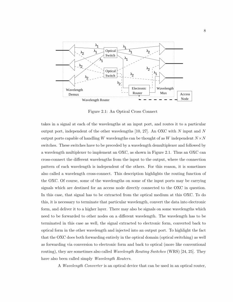
Figure 2.1: An Optical Cross Connect
takes in a signal at each of the wavelengths at an input port, and routes it to a particular
output port, independent of the other wavelengths [10, 27]. An OXC with N input and N
output ports capable of handling W wavelengths can be thought of as W independent N×N
switches. These switches have to be preceded by a wavelength demultiplexer and followed by
a wavelength multiplexer to implement an OXC, as shown in Figure 2.1. Thus an OXC can
cross-connect the different wavelengths from the input to the output, where the connection
pattern of each wavelength is independent of the others. For this reason, it is sometimes
also called a wavelength cross-connect. This description highlights the routing function of
the OXC. Of course, some of the wavelengths on some of the input ports may be carrying
signals which are destined for an access node directly connected to the OXC in question.
In this case, that signal has to be extracted from the optical medium at this OXC. To do
this, it is necessary to terminate that particular wavelength, convert the data into electronic
form, and deliver it to a higher layer. There may also be signals on some wavelengths which
need to be forwarded to other nodes on a different wavelength. The wavelength has to be
terminated in this case as well, the signal extracted to electronic form, converted back to
optical form in the other wavelength and injected into an output port. To highlight the fact
that the OXC does both forwarding entirely in the optical domain (optical switching) as well
as forwarding via conversion to electronic form and back to optical (more like conventional
routing), they are sometimes also calledWavelength Routing Switches (WRS) [24, 25]. They
have also been called simply Wavelength Routers.
A Wavelength Converter is an optical device that can be used in an optical router,

9
λ
λ1λ2
3
λ1
λ
λ2
3
λ1
λ
λ2
3
λ1
λ
λ2
3
λ
λ1λ2
3
λ1
λ
λ2
3
λ1
λ
λ2
3
λ1
λ
λ2
3(a) No Conversion (b) Fixed Conversion
(c) Limited Conversion (d) Full Conversion
Figure 2.2: Wavelength Conversion
to convert the wavelength a channel is being carried on [26]. Without wavelength conversion,
an incoming signal from port pi on, say, the wavelength λ1 can be optically switched (without
intermediate optoelectronic conversions) to any port pj , but only on the wavelength λ1.
With wavelength conversion capability, this signal could be could be optically switched to
any port pj on any wavelength λk. That is, wavelength conversion allows a clear optical
channel to be carried on different wavelengths on different physical links. Different levels
of wavelength conversion capability are possible. Figure 2.2 illustrates the differences for a
single input and single output port situation; the case for multiple ports is more complicated
but similar. Full wavelength conversion capability implies that any input wavelength may
be converted to any other wavelength. Limited wavelength conversion denotes that each
input wavelength may be converted to any of a specific set of wavelengths, which is not the
set of all wavelengths for at least one input wavelength. A special case of this gives us fixed
wavelength conversion, where each input wavelength is converted to exactly one wavelength.
If each wavelength is “converted” only to itself, then we have no conversion. If a node has
limited or full wavelength conversion capability, then the conversion to be effected can be
configured as part of the virtual topology design. The advantage of wavelength conversion is
that the virtual topology that can be implemented is less constrained, since the wavelength
continuity constraint is removed. Thus wavelength use is more efficient. However, the use
of converters increases cost, as well as the complexity of the problem. The cost increase
can be minimized by using limited conversion rather than full conversion, and assuming
a small number of converters rather than conversion capability in every node. But these
assumptions introduce the problems of specifying the nature of the limited conversion and

10
placement of converters in the network, which greatly increase the difficulty of topology
design.
The virtual topology designed and implemented on a physical network not only
determines the performance of the network in terms of metrics like throughput, but also
carries an associated cost, determined by how many and what network components are used
to implement that virtual topology. Attempting to model the network cost is a related field
to the virtual topology design problem. The primary goal of such studies is to provide an
idea of the comparative impacts of various system components on system cost, and hence
provide guidelines for economically efficient virtual topology design, rather than actually
determine the cost of implementing a virtual topology. Comparatively few studies have
been undertaken in this area (see [3] for such a study). Guidelines that result from such
studies may relate to choosing some initial parameters for the virtual topology, as suggested
in [3], or may be integrated into the optimization procedure to find the virtual topology.
The latter approach is taken in [7], where a heuristic is designed for the topology design
problem with a goal of maximizing wavelength utilization in the Wavelength Routers, which
would certainly have an impact on the cost of the virtual topology.
2.1.2 Notation
In this section, we define some terminology and notation and introduce some concepts which
will be used in the following sections, and which are common to most formulations of the
virtual topology problem.
Physical Topology A graph Gp(V,Ep) in which each node in the network is a vertex,
and each fiber optic link between two nodes is an arc. Each fiber link is also called
a physical link, or sometimes just a link. The graph is usually assumed to be
undirected, because each fiber link is assumed to be bidirectional. There is a weight
associated with each of the arcs which is usually the fiber distance or propagation
delay over the corresponding fiber.
Lightpath A lightpath, as we remarked above, is a clear optical channel between two
nodes. That is, traffic on a lightpath does not get converted into electronic forms at
any intermediate nodes, but remains and is routed as an optical signal throughout.
With the usual wavelength continuity constraint, the lightpath becomes a sequence of

11
physical links forming a path from source to detination, along with a single wavelength
which is set aside on each of these links for this lightpath.
Virtual Topology A graph Gv(V,Ev) in which the set of nodes is the same as that of the
physical topology graph, and each lightpath is an arc. It is also called the logical
topology, and the lightpaths are also called logical links. Usually this graph is
assumed to be directed, since a lightpath may exist from node A to node B while there
is none from node B to node A. This graph may also be weighted, with the lightpath
distance of each lightpath (see below) acting as the weight of the corresponding arc.
Link Indicator Whether a physical link exists in the physical topology from a node l to
another node m, denoted by plm which is 1 if such a link exists in the physical topology
and 0 if not.
Lightpath Counter The number of lightpaths that exist from a node i to another node j,
denoted by bij . In many formulations, it is assumed that such a lightpath, if it exists,
is unique, that is a maximum of one lightpath can exist from node i to node j. In
such case, bij is called the lightpath indicator, and is restricted to one of two values, 1
if such a lightpath exists in the virtual topology and 0 if not.
Lightpath Distance The propagation delay over a lightpath, denoted by dij for the light-
path from node i to node j. It is the sum of the propagation delays over the physical
links which make up the lightpath in the virtual topology.
Physical Degree The physical degree of a node is the number of physical links that di-
rectly connect that node to other nodes.
Virtual Degree The virtual (or logical) degree of a node is the number of lightpaths
connecting that node to other nodes. The number of lightpaths originating and ter-
minating at a node may be different, and we denote them by virtual out-degree and
virtual in-degree respectively. We speak simply of the virtual degree if these are as-
sumed to be equal, as they often are. If this degree is assumed to be same for all nodes
of the network, then this is called the virtual degree of the network. The virtual degree
is determined in part by the physical degree, but is also affected by the consideration
of what volume of electronic switching can be done at a node [27], and affects the cost

12
of the topology, since it determines to some extent the number of LTE’s that would
be needed.
Physical Hops The number of physical links that make up a lightpath is called the phys-
ical hop length of that lightpath.
Logical Hops The number of lightpaths a given traffic packet has to traverse, in order to
reach from source to destination node over a particular virtual topology, is called the
virtual or logical hop length of the path from that source to that destination in that
virtual topology.
Traffic Matrix A matrix which specifies the average traffic between every pair of nodes
in the physical topology. If there are N nodes in the network, the traffic matrix is an
N ×N matrix T = [t(sd)], where t(sd) is the average traffic from node s to node d in
some suitable units, such as arriving packets per second, or a quantized bandwidth
requirement. This matrix provides in numerical terms the nature of how the total
network traffic is distributed between different source-destination node pairs, that is,
the pattern of the network traffic.
Virtual Traffic Load When a virtual topology is established on a physical topology, the
traffic from each source node to destination node must be routed over some lightpath.
The aggregate traffic resulting over a lightpath is the load offered to that logical link.
If a lightpath exists from node i to node j, the load offered to that lightpath is denoted
by tij . The component of this load due to traffic from source node s to destination
node d is denoted by t(sd)ij . The maximum of the logical loads is called the congestion,
and denoted by tmax = maxi,j tij .
Physical Loading of a Link This term is used to indicate, for each physical link, the
number of lightpaths that are required to traverse that link in the virtual topology.
2.1.3 Architecture
In this section we characterize in more detail the WDM wavelength routed network we have
been describing above, and which Figure 1.1 illustrates. The network consists of several
routing nodes which are connected to each other by point-to-point optical fibers. The nodes
and their physical connections are specified by the physical topology. Each of the routing

13
nodes may have access nodes connected to it. For the purposes of virtual topology design,
however, only the aggregate traffic between routing nodes is important. Thus we can assume
that each routing node has exactly one access node connected to it. We concentrate on the
routing nodes and refer to them simply as nodes. The traffic matrix specifies the aggregate
traffic from every node to each of the other nodes.
The fiber links connecting the nodes each support a specific number of wavelengths,
say W . Each of the nodes is equipped with a WR capable of routing these W wavelengths.
In general, no wavelength conversion capability is assumed to exist at any of the nodes.
Every physical link carries at most one channel (lightpath) in each direction on each of the
W wavelengths.
Lightpaths are set up on the physical topology, creating the virtual topology. Each
arc of the virtual topology graph is a lightpath. A lightpath is set up by configuring the
source and destination nodes to originate and terminate a specific wavelength, then choosing
a path from the source to destination node and configuring the WR at each intermediate
node on that path to forward that wavelength optically to the next node. Thus at the
intermediate nodes the traffic is not converted to electronic form, and the lightpath acts
as a single-hop path from source to destination, or a pipe, with no queuing delay. Two
lightpaths that share a physical link must be assigned different wavelengths. The total
number of wavelengths used on a certain link must be W or less. The logical in-degree
and out-degree are usually equal for each node. The logical degree of every node is usually
assumed to be the same and this is called the logical degree of the network.
Traffic is routed from each source to destination node over a single lightpath if
one exists for that source and destination, or a sequence of more than one ligthpaths or
logical hops. It is usually assumed to simplify the optimization problem that traffic for
a single source-destination pair may be bifurcated over different virtual routes. The aim
of creating the virtual topology is to ensure that more traffic can be carried with fewer
optoelectronic conversions along the way. The extreme case of this would be if a lightpath
could be set up from each source to each destination; however, the number of wavelengths
available is usually too limited to allow this. At the other extreme is a virtual topology
which is identical to the physical topology, so that optoelectronic conversion occurs at
every intermediate node. With reasonable and achievable virtual topologies, the number
of optoelectronic conversions should not be very large. Together with the fact that in high
speed wide area networks the propagation delay dominates over the queueing delay (as long

14
as links are not loaded close to capacity), queueing delays are typically neglected in the
problem formulation [27].
The goal of the virtual topology design process is usually to optimize network
performance, such as minimize network congestion or minimize average packet delay. In
the optimization, usually the number of wavelengths available is taken as a constraint.
If both minimizations are desired, then one of them is usually expressed as a constraint
by relating it to a known physical network characteristic. In general both are important
because too little emphasis placed on the congestion aspect usually results in a virtual
topology very similar to the physical topology, and too little emphasis placed on the delay
aspect can result in virtual topologies which bear little resemblance to the physical topology,
with convoluted lightpaths that increase delay [27].
2.2 Network Performance Optimization
In this section we provide an exact formulation of the virtual topology design problem using
the packet traffic approach, and discuss specific techniques and heuristics, used to solve it.
2.2.1 Formulation
The exact formulation of the virtual topology problem is usually given as a Mixed Integer
Linear Program. The formulation provided here follows closely that in [19], and also those in
[27, 24, 25]. The symbols and terminology are as defined in Section 2.1.2. New terminology
is defined as necessary.
Additional Definitions
Let H = [hij ] be the allowed physical hop matrix, where hij denotes the maximum
number of physical hops a lightpath from node i to node j is allowed to take. This hop
matrix is one of the ways to characterize the bounds which lightpaths in the virtual topology
must be within. Let c(k)ij be the lightpath wavelength indicator, i.e. c
(k)ij is 1 if a
lightpath from node i to node j uses the wavelength k, 0 otherwise. Let c(k)ij (l,m) be the
link-lightpath wavelength indicator, to indicate whether the lightpath from node i to
node j uses the wavelength k and passes throught the physical link from node l to node m.
Let ∆l denote the logical degree of the virtual topology.

15
Objective
Minimize the congestion of the network, that is,
min tmax (2.1)
Subject to:
Degree Constraints
∑j
bij ≤ ∆l, ∀i (2.2)
∑j
bji ≤ ∆l, ∀i (2.3)
Traffic Constraints
tij ≤ tmax, ∀(i, j) (2.4)
tij =∑sd
t(sd)ij , ∀(i, j) (2.5)
t(sd)ij ≤ bijt
(sd), ∀(i, j), (s, d) (2.6)
∑j
t(sd)ij −
∑j
t(sd)ji =
t(sd), s = i
−t(sd), d = i
0, s �= i, d �= i
∀(s, d), i (2.7)
Wavelength Constraints
W−1∑k=0
c(k)ij = bij , ∀(i, j) (2.8)
c(k)ij (l,m) ≤ c
(k)ij , ∀(i, j), (l,m), k (2.9)∑
ij
c(k)ij (l,m) ≤ 1, ∀(l,m), k (2.10)
W−1∑k=0
∑l
c(k)ij (l,m)plm −
W−1∑k=0
∑l
c(k)ij (m, l)pml =
bij , m = j
−bij , m = i
0, m �= i,m �= j
∀(i, j),m
(2.11)

16
Hop Constraints ∑lm
c(k)ij (l,m) ≤ hij , ∀(i, j), k (2.12)
Discussion
The degree constraints (2.2) and (2.3) constrain the virtual topology to a given logical de-
gree. Among the traffic constraints, (2.4) defines the network congestion. Expression (2.5)
asserts that the total traffic on a lightpath is the sum of the traffic components on that light-
path due to all the different pairs of source and destination nodes. Constraint (2.6) captures
the fact that the component of traffic on a lightpath due to a particular source-destination
pair can be present only if the lightpath exists in the virtual topology, and cannot be more
than the total traffic for that source-destination pair. Constraint (2.7) is an expression of
the conservation of traffic flow at lightpath endpoints. All but one of the remaining con-
straints relate to the allocation of wavelengths to lightpaths. Constraint (2.8) ensures that
a lightpath, if it exists in the virtual topology, has a unique wavelength out of the available
ones. Constraint (2.9) enforces the consistency of the lightpath wavelength indicators and
the link-lightpath wavelength indicators, and expression (2.10) enforces that a wavelength
can be used at most once in every physical link, avoiding a wavelength clash. Expression
(2.11) asserts the conservation of every wavelength at every physical link endpoint for each
lightpath. The last remaining constraint, expression (2.12), enforces the bounds on the
number of physical hops each lightpath is allowed.
The parameters, or inputs, to the formulation are the traffic matrix T , the hop
bound matrix H, the number of wavelengths supported by a fiber W , the desired logical
degree ∆l, and the details of the physical topology graph. The variables, whose values at
optimum are the “output” of the MILP, relate to the virtual topology graph, wavelength
assignment in the virtual topology, and the traffic routing over the virtual topology. The
lightpath indicators bij provide the virtual topology graph. The lightpath wavelength and
link-lightpath wavelength indicators provide the wavelength assignments to the lightpaths
in the virtual topology and also the physical links used to implement each lightpath. Lastly,
the virtual traffic load variables tij and t(sd)ij provide the routing of the traffic between each
source and destination on the virtual topology.
Formulations of this problem are possible that address only some and not all of
these aspects. In Section 3.2 we discuss such approaches. Even when all these aspects
17
are addressed, or the same aspect is addressed, different formulations of the problem are
possible.
The above formulation assumes that lightpath indicators are used instead of light-
path counters. If lightpath counters are used, this formulation can be used unchanged if
it is assumed that all lightpaths from a given source node i to a given destination j must
traverse the same sequence of physical links; however, this is not a very reasonable assump-
tion in general. The formulation can be enhanced to allow more general approaches using
lightpath counters.
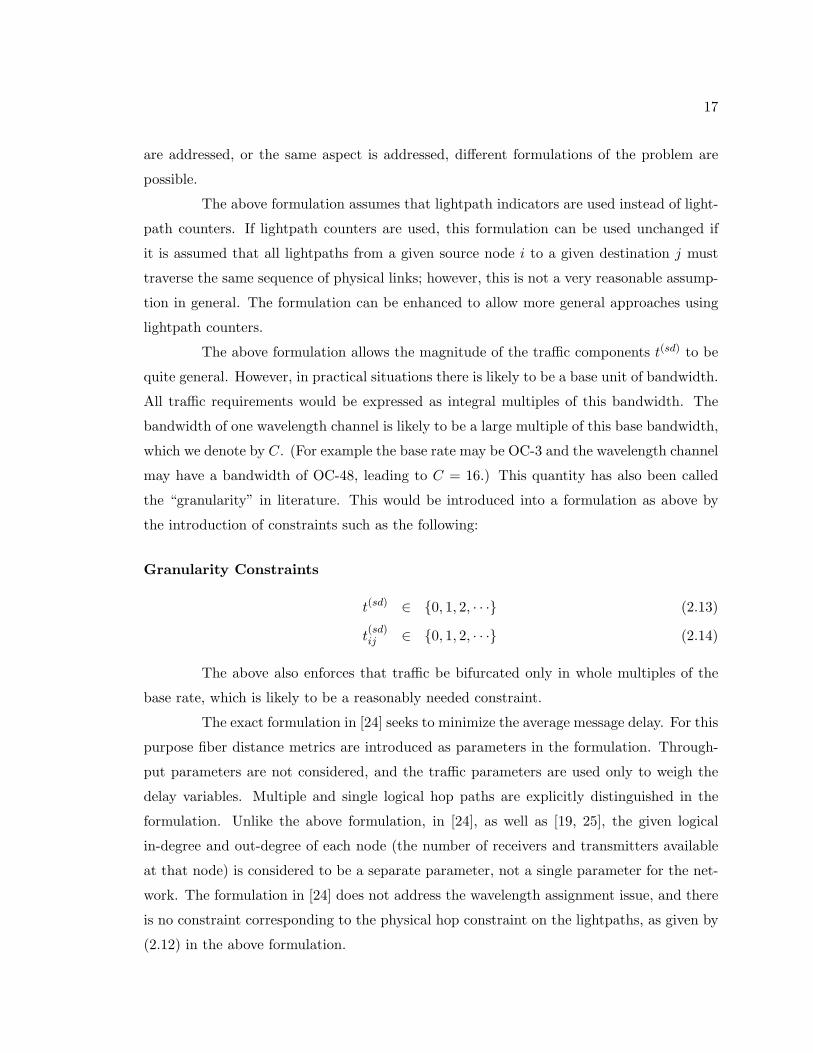
The above formulation allows the magnitude of the traffic components t(sd) to be
quite general. However, in practical situations there is likely to be a base unit of bandwidth.
All traffic requirements would be expressed as integral multiples of this bandwidth. The
bandwidth of one wavelength channel is likely to be a large multiple of this base bandwidth,
which we denote by C. (For example the base rate may be OC-3 and the wavelength channel
may have a bandwidth of OC-48, leading to C = 16.) This quantity has also been called
the “granularity” in literature. This would be introduced into a formulation as above by
the introduction of constraints such as the following:
Granularity Constraints
t(sd) ∈ {0, 1, 2, · · ·} (2.13)
t(sd)ij ∈ {0, 1, 2, · · ·} (2.14)
The above also enforces that traffic be bifurcated only in whole multiples of the
base rate, which is likely to be a reasonably needed constraint.
The exact formulation in [24] seeks to minimize the average message delay. For this
purpose fiber distance metrics are introduced as parameters in the formulation. Through-
put parameters are not considered, and the traffic parameters are used only to weigh the
delay variables. Multiple and single logical hop paths are explicitly distinguished in the
formulation. Unlike the above formulation, in [24], as well as [19, 25], the given logical
in-degree and out-degree of each node (the number of receivers and transmitters available
at that node) is considered to be a separate parameter, not a single parameter for the net-
work. The formulation in [24] does not address the wavelength assignment issue, and there
is no constraint corresponding to the physical hop constraint on the lightpaths, as given by
(2.12) in the above formulation.

18
In [27], the bound on the number of wavelengths a single fiber can carry is ignored
in the exact formulation. The wavelength assignment problem is also not addressed. The
physical hop bound is not used to constrain the virtual topology, instead there is an av-
erage delay constraint on each source-destination pair. The maximum propagation delay
between any source-destination pair in the physical topology is denoted by d(max) and in-
troduced in the formulation, together with a tuning factor α which determines how tightly
the virtual topology should be constrained by d(max). The average packet delay for each
source-destination pair is constrained to be less than or equal to the product of α and d(max).
Thus the delay performance metric is addressed using a constraint such as the following:
Delay Constraints ∑ij
t(sd)ij ≤ t(sd)αd(max), ∀s, d (2.15)
The throughput performance metric is addressed by the goal of the optimization,
which is to minimize congestion as in the formulation provided above.
The exact formulation in [25] follows the exact formulation in [24], but adds some
elements. The capacity of each lighpath C is introduced as a parameter and it is used
to refine the delay minimization goal and to set up an alternative optimization goal of
maximizing the offered load to the network. The second goal is non-linear in nature. The
wavelength assignment problem is made part of the exact formulation.
In [3], the formulation is similar to the one we have provided above, but a simplifi-
cation is introduced as part of the formulation. The goal of the optimization is to minimize
the average physical hop lengths of the lightpaths in the virtual topology. The wavelength
continuity constraint is not included. The lightpath distance is constrained to be bounded
by the fiber distance of the shortest path in the physical topology between the endpoints
of that lightpath, together with a factor α introduced as a parameter. The simplification
consists of pruning the search space based on the fiber length of paths: lightpaths are only
allowed to use physical paths which are among the K shortest such paths between any pair
of nodes, K being a parameter in the problem formulation.
Some common features of the exact formulations from various studies in the lit-
erature are also shared by the formulation provided above. Bifurcation of traffic for a
source-destination pair over different virtual paths is allowed. In view of the predominance
of propagation delay over queueing delay in high speed wide area networks, the queueing

19
delay is neglected in almost every formulation of the problem. A special parameter β is
introduced in [3] to bound the congestion to values at which it is reasonable to neglect
queueing delays. The formulation provided above also has a specific feature not shared
by all the others in that it does not allow for more than one lightpath from one node to
another.
As we discuss in Section 2.2.2, this formulation gets quickly intractable with size.
One of the ways it can be made more tractable is to aggregate traffic from a given source node
to all destination nodes, that is, not formulate the problem in terms of the traffic components
between each source-destination pair t(sd), but traffic components for each source node t(s)
only. This results in a more tractable formulation because the number of variables and
constraints is lower, otherwise the formulation is similar. Of course, the solution to the
problem so formulated does not provide a complete solution to the full problem in terms
of routing traffic over the virtual topology designed, moreover there may not be a feasible
solution to the original problem corresponding to a solution for the aggregate problem.
However, the aggregate problem, being less constrained than the original one, helps set
achievability bounds on the full problem, such as lower bounds on the achievable congestion
[27, 19]. Bounds which can be calculated with significantly lower computational costs than
solving the full problem are useful in evaluating heuristics employed to obtain good solutions
to the full problem, as discussed in Section 2.2.2.
Usually, such an aggregate formulation is used after relaxing the MILP above
into an LP, that is allowing the lightpath, lightpath wavelength and link-lightpath wave-
length indicator variables to take up values from the continuous interval [0, 1] rather than
constraining them to be binary variables. The relaxation, like the aggregate formulation,
results in a less constrained formulation, and hence is suitable for deriving achievability
bounds. When the MILP is relaxed, an extra “cutting plane” constraint is introduced
[27, 19], to ensure that the definition of congestion remains consistent with the MILP for-
mulation when traffic components may be weighted with the “fractional lightpaths” that
the relaxation introduces.
2.2.2 Heuristics
An exact formulation of this problem such as the one given in Section 2.2.1 quickly grows
intractable with increasing size of the network. In fact, this problem and some of its

20
subproblems are known to be NP-hard [9, 24, 19, 2]. Thus for networks of moderately large
sizes it is not practical to attempt to solve this problem exactly. Heuristics to obtain good
approximations are needed. In the rest of this section we discuss heuristic approaches to
the virtual topology design problem or to related subproblems.
Subproblems
The full virtual topology design problem can be approximately decomposed into four sub-
problems. The decomposition is approximate or inexact in the sense that solving the sub-
problems in sequence and combining the solutions may not result in the optimal solution
for the fully integrated problem, or some later subproblem may have no solution given the
solution obtained for an earlier subproblem, so no solution to the original problem may be
obtained. Although this decomposition follows [25], it is also consistent with the decompo-
sitions of [27, 24, 19, 2]. The subproblems are as follows.
1. Topology Subproblem: Determine the virtual topology to be imposed on the phys-
ical topology, that is determine the lightpaths in terms of their source and destination
nodes.
2. Lightpath Routing Subproblem: Determine the physical links which each light-
path consists of, that is route the lightpaths over the physical topology.
3. Wavelength Assignment Subproblem: Determine the wavelength each lightpath
uses, that is assign a wavelength to each lightpath in the virtual topology so that
wavelength restrictions are obeyed for each physical link.
4. Grooming (or Traffic Routing) Subproblem: Route packet traffic between
source and destination nodes over the virtual topology obtained.
In terms of the formulation provided in Section 2.2.1, the topology subproblem
consists of determining the values of the lightpath indicator variables bij , the lightpath
routing subproblem consists of determining the values of the variables c(k)ij (l,m), the wave-
length assignment suproblem consists of determining the values of the variables c(k)ij , and the
traffic routing subproblem consists of determining the values of the variables t(sd)ij . It may be
noted that the above description of the lightpath routing subproblem is approximate since
fixing the values of the variables c(k)ij (l,m) would entail specifying wavelengths for each

21
lightpath, that is solving the wavelength assignment subproblem as well. The lightpath
routing subproblem actually consists only of determining values of link-lightpath indicators
(not included in the above formulation) and does not refer to wavelength assignment in any
way.
The traffic routing subproblem may appear to be not essential to the virtual topol-
ogy design issue. Indeed, once the virtual topology is fixed by solving the first three sub-
problems, the traffic routing subproblem is the known one of routing traffic over a given
topology, for which many algorithms exist. This is true when we are concerned only with
specific optical characteristics of the topology, such as the number of wavelengths needed.
However, as we have mentioned above, it is now recognized that grooming of traffic is of
primary importance since it affects the cost of the network as well as performance (by re-
ducing the necessity of electronic processing and hence loss). Thus traffic grooming is not
only integral to the problem but central to it.
As we remarked above, the decomposition into subproblems is inexact and hence
attempting to solve the subproblems and combine the solutions may result in a suboptimal
solution or even no solution to the full problem. Exact solution of all the subproblems is
also not possible since some of the subproblems are NP-hard as well. Heuristics must be
employed to obtain good solutions to the subproblems. This also leads to the possibility
of obtaining no solution to the full problem. Some constraints are usually relaxed so that
at least some solution is obtained from the heuristics, which can be then tested for near
optimality using achievability bounds as we discuss in the following section. One of the
constraints which is commonly relaxed is that of the maximum number of wavelengths that
can be carried by a fiber. Of course, if after the solution is obtained we find that some of
the relaxed constraints have been violated (for example, if we have assigned a link to carry
more lightpaths than the maximum number of wavelengths it can carry, or the total number
of unique wavelengths used in the virtual topology is more than the maximum number of
wavelengths a fiber can carry) then we would need to abandon that solution and search for
a different one, possibly after modifying the heuristics used.
The virtual topology problem can be decomposed into different subproblems than
the ones we list above. Such different decompositions are used in many of the studies
we survey. However, we consider the above decomposition to be reasonable and fairly
consistent with any others proposed in the literature we survey, and we shall refer only to
this decomposition while discussing such studies.

22
Chapter 3
Previous Work
Since the virtual topology problem is recognized to be intractable in general, lit-
erature has been largely concerned with obtaining good bounds and heuristic solutions to
the problem in various contexts. In this chapter, we review and summarize some of the
recent literature in this field, as well as some literature that address issues related to virtual
topology problems.
3.1 Bounds
To evaluate an approximate solution produced by a heuristic, we would like to know how
close the obtained solution is to the optimal one. Since we are using the heuristic because
of the very reason that the optimal solution cannot be obtained in the first place, we must
resort to comparing the solution obtained with known bounds on the optimal solutions
derived from theoretical considerations. These are the achievability bounds we have men-
tioned before (so called because they are bounds on what can be achieved in principle) and
we discuss them below.
3.1.1 Lower Bounds on Congestion
The goal of virtual topology design is often to minimize network congestion, as in our
formulation in Section 2.2.1. A lower bound on the congestion obtained from theoretical
considerations allows us to know that an even smaller value of congestion cannot be achieved
by any solution, and helps us evaluate the solution produced by some heuristic. We discuss
several lower bounds on congestion below. Our discussion follows closely that of [27], and

23
also that of [19], as well as literature on virtual topology problems in broadcast LAN
scenarios as referred to in [27, 20]. More details can be found in these sources.
Physical topology independent bound: This bound utilizes the fact that the load on
each logical link would be the same, and this would be the congestion, if the total traffic in
the network were equally distributed among all the lightpaths. The value of this congestion
would then act as a lower bound on any virtual topology that could be designed for the
network under the given traffic conditions. This bound takes into account the total traffic
demand, but not the distribution of total traffic among the different source-destination pairs
(that is, the traffic pattern). As such, it assumes that traffic for any source-destination pair
can be assigned to any lightpath in the virtual topology, and hence, it ignores the physical
topology.
Let H be the traffic weighted average number of logical hops in the virtual topology.
If El denotes the number of lightpaths in the virtual topology and r denotes the total arrival
rate of packets to the network, then it is easy to see that
tmax ≥ rH /El (3.1)
Thus, setting a lower bound on H results in a lower bound on the congestion. This is
done from the following consideration. For N nodes in the network and a logical degree
∆l, the maximum number of source-destination node pairs that can be connected by only a
single hop is N∆l. Similarly the maximum number of source-destination pairs that can be
connected by only two hops is N∆2l , by only three hops is N∆3
l , and so on. For the traffic
weighted number of hops to be minimum, source-destination pairs with the largest amount
of traffic must be connected by a small number of logical hops. Accordingly, assume that
the N∆l source-destination pairs with the largest traffic between them are each connected
by a single hop path (that is there is a lightpath between each source and the corresponding
destination). The N∆2l source-destination pairs with the next largest traffic should be
connected by two hop paths, and so on. The traffic weighted average number of logical
hops in this case is a lower bound, in other words
H ≥∑k
kSk (3.2)
where Sk is the sum of the traffic fractions (with respect to total network traffic r) which
comprise the k-th block when the traffic fractions are arranged in descending order of

24
magnitude, and the i-th block is made up of N∆il successive elements in that list.
Minimum flow tree bound: This bound is derived from similar considerations as above,
but on the basis of each source node rather than the network as a whole. In the above we
assumed that the N∆l source-destination pairs are all connected by single hop paths, and
so on, but this is impossible if the ∆l + 1 top traffic components all have the same source
node, for example. In this bound, we take into account the restriction that each source node
can only source ∆l lightpaths altogether, in addition to the considerations above. Thus this
is a stronger bound.
The calculation of this bound is done by assuming that for each source, the source
is connected by one logical hop to the ∆l destinations to which it has the largest amounts
of traffic, by two hops to the ∆2l destinations to which it has the next largest amounts
of traffic, and so on. We then form the sum of these traffic components weighted by the
appropriate number of hops, as in the above scheme, and obtain the bound for the traffic
weighted average number of logical hops H, similar to (3.2). The bound on congestion is
then obtained from (3.1), as before. We omit the derivation and exact expression of this
bound, which can be found in [27].
Iterative bound: This type of bound is developed in [27, 19] by aggregating and then
relaxing the MILP formulation and solving it as mentioned in Section 2.2.1. The additional
constraint imposed on the relaxed aggregate formulation is that the congestion be higher
than a lower bound on the congestion known a priori, such as the minimum flow tree
bound discussed above. To improve the tightness of the bound, the value obtained for the
congestion by solving the relaxed aggregate LP can be used as a new value of the a priori
bound and the LP solved again to yield a further improved bound on the congestion. This
iterative process can be carried out repeatedly to improve the tightness of the bound. It is
remarked in [27] that about 25 iterations result in a bound that is improved very little by
further iterations.
Independent topologies bound: This bound is proposed in [4] as another method of
taking into account the physical topology in computing a bound on the congestion. This
bound is also based on relaxing the MILP formulation to obtain a linear problem. First a
logical feasible virtual topology is obtained that maximizes the one-hop traffic. In the next

25
stage, the traffic carried by this topology is eliminated from the total traffic and another
virtual topology is designed which carries the maximum possible two-hop traffic out of the
residual traffic. This procedure is repeated for successive number of hops until all the traffic
is routed. The value of congestion can now be extracted from the several topologies. If
this procedure were carried out exactly, it would be an exact solution and would not be
more easily computable than a solution to the problem itself. However, the several logical
topologies are not allowed to constrain each other, so that the topologies for more than
one hop are not necessarily feasible. Thus the topologies are mutually independent. The
authors of [4] note that this bound is only a little tighter than the flow tree based bound if
traffic is uniform, but becomes much tighter for highly nonuniform traffic.
3.1.2 Lower Bounds on the Number of Wavelengths
It is usually necessary in virtual topology design to complete the design using as few distinct
wavelengths as possible, since in practice there is a limit on the number of wavelengths a
fiber can carry. This limit may be known and introduced in the exact formulation as in the
formulation of Section 2.2.1, but such a limit is often not included in heuristic approaches.
A lower bound on the number of wavelengths needed for a particular problem is then useful
in evaluating the solution provided by the heuristic. Also, in the presence of practical
limitations, an easy to compute lower bound on the number of wavelengths can provide a
quick negative answer to the question of whether a virtual topology design problem is at
all feasible or not. Two such bounds, following [27], are discussed below.
Physical topology degree bound: This bound is derived from the simple consideration
that each node in the virtual topology must source a number of lightpaths equal to the logical
degree of the virtual topology ∆l. Considering the node with the minimum physical degree
δp in the physical topology, there must be a sufficient number of wavelengths to allow ∆l
lightpaths to be realized over δp physical links, that is the number of wavelengths required
is bound from below by W ≥ ∆l/δp�.
Physical topology links bound: Another consideration is that each physical link is
traversed in general by multiple lightpaths in each direction. If we count each physical link
once every time a lightpath traverses it, then the total will be greater than the number of
directed physical links in the topology (we multiply the number of links in the undirected

26
physical topology by two to get this latter number). This is possible because different
lightpaths on the same physical link (in the same direction) use different wavelengths. Thus
the average number of lightpaths traversing a physical link can be obtained by dividing the
total number of physical links traversed by all the lightpaths by the number of directed
physical links in the topology, and this is a bound on the number of wavelengths required.
For the number of physical links traversed by all the lightpaths, we use the following
argument. For each source node, reaching every other node requires a minimum number of
physical hops, using the shortest physical path. Let us list the N − 1 possible destination
nodes for a source node ni in increasing order of the number of physical hops needed to
reach that destination from ni, and then assume that the ∆l lightpaths sourced from ni
traverse the ∆l physical paths which lead to the first ∆l destinations on that list. We
assume this is true for each source node ni. This assumption results in a lower bound on
the total number of physical links traversed, and hence on the number of wavelengths. We
omit the derivation and exact expression of this bound, which can be found in [27].
Another bound, which is derived with respect to the lightpath routing and wave-
length assignment subproblems and not the complete problem, may nevertheless be useful
in some cases. This is the NWC bound [9] (for Non-Wavelength Continuous) which states
that given a physical topology and a set of lightpaths to be established, the number of
wavelengths needed to establish a virtual topology obeying the wavelength continuity con-
straint is not less than the number needed to establish the same virtual topology without
the wavelength continuity constraint. In general, it is not clear how tight this bound is, and
it is not easily computable. However, it can be shown that for networks with topologies
which are acyclic this bound is not only tight but exact [9]. Thus it could be useful if after
finding a solution to the lightpath routing subproblem we find an acyclic topology and want
a bound to evaluate a heuristic solution to the wavelength assignment subproblem.
Bounds on the number of wavelengths required can also be found under specific
assumptions regarding the solution to the different subproblems. For example, in [10] it is
demonstrated that if the virtual topology being implemented is decided to be a hypercube
(as part of solving the topology subproblem) then for a specific proposed algorithm to map
the hypercube nodes to physical network nodes (solving the rest of the topology subprob-
lem), the number of wavelengths required cannot be less than 23n, where n is the number of
nodes in the physical network. A similar result for a torus embedding, as well as a general
result in terms of the physical topology and the topology being embedded is also provided

27
in [10].
3.2 Heuristic Approaches and Techniques
In the design of heuristics or approximate solutions to the virtual topology problem, em-
phasis is placed on different aspects of the problems by different authors. In the majority of
the literature, heuristics are designed for only some and not all the subproblems. Some as-
sumption regarding the nature of the virtual topology to be implemented is often a starting
point for heuristic methods. Below we discuss heuristics found in the literature surveyed
under three different categories. In the first, it is assumed that the virtual topology to be
implemented is a well-known regular topology, such as a hypercube or a shufflenet. In the
second, the lightpaths of the virtual topology are assumed to be already known in terms of
sources and destinations for each instance of the problem, and the lightpath routing and
wavelength assignment subproblems are addressed. No particular assumption is made re-
garding the virtual topology in the last category. Some of the interest in the study of regular
topologies in the context of virtual topologies for WANs came from the assumption that to
some extent the virtual topology could dictate the physical topology, that is, fibers could
be laid to supplement a physical topology before implementing a virtual topology. As more
and more fiber has been laid in practice and has become part of single wavelength optical
networks utilizing the fibers as point-to-point links, the concern has shifted to extracting
more utilization out of these fibers using WDM and virtual topologies, rather than having
to lay more fibers. Thus studies relating to arbitrary physical topologies have attracted
more interest in recent times.
3.2.1 Regular Topologies
Regular topologies such as hypercubes or shufflenets have several advantages as virtual
topologies. They are well understood, and results regarding bounds and averages are com-
paratively easier to derive. Routing of traffic on a regular topology is usually also simpler
and results are available in the literature, so the traffic routing subproblem usually becomes
trivial. Also, regular topologies possess inherent load balancing characteristics.
Once a regular topology is decided upon as the one to be implemented as a virtual
topology, it remains to decide which physical node will realize each given node in the regular
topology (this will be referred to as the node mapping subproblem) and which sequence of

28
physical links between two physical nodes will be used to realize each given edge in the
regular topology, that is, lightpath (this will be called the path mapping subproblem). This
procedure is also called embedding a regular topology in the physical topology. In terms
of the subproblems introduced in Section 2.2.2, the choice of the regular topology together
with the node mapping problem make up the virtual topology subproblem, and the path
mapping problem corresponds to the lightpath routing subproblem. Obviously, the number
of nodes in the regular topology may not be chosen with complete freedom, instead it must
obey the constraints of the regular topology. For example, the number of nodes in a torus
must obey n = m2 for some m. In case the physical topology has a few nodes less than the
regular topology, this can usually be circumvented by adding fictitious nodes to it before
embedding [24]. If a few more nodes are present in the physical topology, then some of the
ones with less traffic may be combined for the purpose of embedding, though this introduces
further approximations to the virtual topology solutions. In general, the node mapping and
path mapping problems leave out of consideration the traffic patterns in the network, and
utilize metrics such as fiber distances and wavelength reuse to route lightpaths over the
physical topology. Thus there is a tacit assumption of reasonably uniform traffic pattern in
the use of regular topologies as virtual topologies.
The mappings must also be free of wavelength clashes and must obey any pre-
defined limit on the number of wavelengths. These problems are themselves known or
conjectured to be NP-hard [10, 24], hence heuristics are needed for them. Below we discuss
some approaches taken in the literature with regular topologies as candidates for virtual
topologies.
Embedding via strings: In [10], the authors propose a two-phase heuristic for perform-
ing the mappings. In the first phase, an “equivalent” string is obtained for the physical
network. In the second phase, the selected regular topology is embedded into the string.
The elements listed in the string represent the nodes of the physical topology. Each edge
connecting two successive elements of the string corresponds to a path between the corre-
sponding nodes. The string also has the property that any two paths that are edge disjoint
in the string are also edge disjoint in the physical topology, so that path mapping and
wavelength allocation on the string can be translated in a straightforward manner to the
physical topology.
Three methods of obtaining such a string representation from a physical topology

29
are discussed in [10]. The first two involve finding a Hamiltonian path and an Eulerian
path in the physical topology. However, there is no guarantee that such paths can be found
in an arbitrary physical topology, and hence these methods are not completely general,
though they have other attractive characteristics. The third method involves finding a
spanning tree in the physical topology, which only requires that the topology graph be
connected. Algorithms for embedding a torus topology and a hypercube topology into these
string representations are then presented. A general result regarding a lower bound on the
number of wavelengths needed to embed an arbitrary topology Ge on another topology Gg
is then derived in terms of characteristics of Ge and Gg, and this result is used to derive
lower bounds for the torus and the hypercube cases. The resulting virtual topologies are
compared in terms of logical degree of the network, average number of logical hops, and
the number of wavelengths needed. The hypercube embedding is seen to have the better
(i.e., smaller) number of logical hops, but it requires a larger network degree and more
wavelengths. It appears that algorithms can be similarly developed for embedding other
regular topologies in the string representations.
The approximation in this approach is introduced at the time of obtaining a string
representation. The string obtained is constrained by only the criteria mentioned above,
and this does not guarantee that the particular string we obtain for a given instance will lead
us to an optimal or near-optimal virtual topology. However, given the regular topology to
be embedded and the embedding function, it is shown in [10] that the particular algorithms
presented are near-optimal. In this approach, the traffic pattern in the network is ignored.
Comparison of topologies: Three different regular topologies are compared for their
suitability as virtual topologies in [22]. The comparison is based on the number of logical
hops between nodes and the number of wavelengths required. No traffic pattern considera-
tions are included. In fact this comparison does not refer to a physical network at all. The
regular topologies are looked upon only as candidates for embedding into physical topolo-
gies, and it is assumed that the required node mapping and path mapping may be carried
out. In this sense this study is from the perspective of the first part of the virtual topology
subproblem, in that the virtual topology is proposed but node mappings are not performed.
However, this study addresses the issue of wavelength routing given the virtual topology,
which provides the path mapping.
The three topologies compared are the K-grid topology (an extension to K di-

30
mensions of the Manhattan Street topology), the twin shuffle topology (a shufflenet with
twice the connectivity, that is two shufflenets in parallel), and a modified de Bruijn graph
(de Bruijn graphs with connectivity multiplied by a factor). The basis of comparison is the
degree of the network. However, this is expressed as the number of bundles of fiber leaving
each node, where each bundle carries fibers to exactly one other node but may contain more
than one fiber. Thus, the allowed number of wavelengths along a connection between two
nodes would be larger with this scheme than with a single fiber scheme. This difference
is expressed by a difference between the number of wavelengths required to implement the
virtual topology and a normalized version of the same number.
The authors point out that the de Bruijn graph topology has the advantage of a
constant number of hops between nodes, and this number is smaller than either the average
or maximum number of hops for the other two topologies. The number of wavelengths
required appear to be similar for the three topologies.
Simulated Annealing: In [24], heuristics are developed for the node mapping problem
for regular topologies (specifically, hypercubes), and the solution is carried through to path
mapping as well as wavelength assignment. Thus, the node mapping part of the virtual
topology subproblem, the lightpath routing, and the lightpath wavelength assignment sub-
problems are addressed. Moreover, the nature of the physical topology is taken into account
to some extent. The goal of each heuristic is to minimize overall average message delay in
the virtual topology, which involves the fiber distances and the traffic pattern in the net-
work. Two heuristic approaches are developed, one based on a greedy algorithm and the
other on simulated annealing.
In both approaches, fictitious nodes are created in the physical topology if it has
fewer nodes than the chosen hypercube. The greedy approach starts with a reasonable
initial node mapping obtained by mapping the nodes with the highest physical degrees
first and attempting to map nodes so that logical nodes that are neighbors in the logical
topology are mapped to physical nodes that are neighbors in the physical topology as far
as possible. This node mapping is then refined by traversing the list of nodes in reverse
order of initial embedding and swapping each with a different node if this would reduce
the average message delay. Once the final node mapping is obtained, the path mapping
is obtained by shortest path routing on the physical topology to realize each edge of the
hypercube, that is, lightpath. A remark is made regarding the traffic routing subproblem

31
that shortest path routing on the hypercube virtual topology has been assumed.
To assign wavelengths, physical links are ordered in decreasing order of number
of lightpaths passing through them. For each physical link, each lightpath is assigned a
different wavelength if it has not already been assigned one through some other physical
link. Wavelength conflicts are avoided while assigning wavelengths. This algorithm is
heuristic in nature and in particular is not guaranteed to find a solution if the number of
wavelengths is bounded, even if a solution exists. With unbounded number of wavelengths,
this algorithm does not impose an obvious non-trivial bound on the number of wavelengths
it uses, and such a bound is not discussed in [24].
In the simulated annealing heuristic, the node mapping process starts with an
initial random mapping. The perturbation is provided by swapping the mapping of two
nodes in the virtual topology. The acceptance criterion is the average message delay in the
network; the new mapping is always accepted if the resulting delay decreases, and is accepted
if the delay increases with a probability that goes down as the simulated temperature falls.
Once the mapping “freezes” the path mapping and wavelength assignment are carried out
as for the greedy algorithm.
In [25], a very similar simulated annealing heuristic is presented, with the difference
that the traffic routing subproblem is assumed to be solved using the flow deviation method.
The flow deviation method is a good heuristic alternative to an exactly optimal linear
programming routing flow solution. The literature in which it was developed is referred to
in [25] and also [20]. This method starts from an initial flow assignment, and iteratively
deviates flows over alternate paths, avoiding links carrying the largest amounts of traffic.
3.2.2 Pre-specified Topologies
In this section we discuss studies which focus on the lightpath routing subproblem, and
possibly the wavelength assignment and traffic routing subproblems. In other words, the
virtual topology in terms of a list of lightpaths with their source and destination nodes
is supposed to be given for each instance of the problem. The traffic pattern in the net-
work, as we have seen, can be used to determine what lightpaths to set up. The traffic
pattern can also be useful in routing the lightpaths and the traffic, because the network
performance metrics which are the goals of the virtual topology design are related to traffic,
such as message delay or congestion. Thus the traffic pattern may be utilized even in an

32
approach focused on the lightpath routing subproblem only. However, in some approaches,
it is considered that the traffic pattern has been properly taken into consideration while
solving the virtual topology subproblem which resulted in the given set of lightpaths to be
implemented, and thus the lightpaths take care of the traffic characteristics of the network.
The lighpath routing and wavelength assignment subproblems can then be viewed as hav-
ing goals defined purely in terms of the lightpaths, such as minimization of the number of
distinct wavelengths needed.
SLE: In [9], not only the source and destination, but also the routing of the lightpaths is
assumed to be given, and the problem is seen to be the assignment of wavelengths to these
lightpaths. That is, the lightpath wavelength assignment subproblem is addressed, and it is
called the Static Lighpath Establishment (SLE) problem. SLE as posed includes a bound
on the number of wavelengths that can be used to establish the lightpahts. It is proved that
SLE as stated is equivalent to the n-graph-colorability problem, and hence NP-complete.
A heuristic algorithm to assign wavelengths to a given set of lighpaths with the
aim of using as few wavelengths as possible is presented. This algorithm is based on a
greedy allocation heuristic which iteratively assigns a wavelength to as many edge disjoint
lightpaths as possible before going on to the next wavelength. Longer lightpaths are allo-
cated a new wavelength earlier. The algorithm terminates when all lightpaths have been
assigned a wavelength. There is no obvious non-trivial bound to the number of wavelengths
needed by this algorithm, and none is discussed in [9]. A modified version of this algorithm
that allocates wavelengths only until a given maximum number of wavelengths have been
allocated, and then stops, is also given. The use of such an algorithm is in deriving values of
blocking probabilities than can be compared with values encountered in the dynamic case.
The problem of dynamic lightpath establishment, in which lightpaths are set up
and torn down on demand, and the goal is to provide the minimum blocking probability
seen by new lightpath demands, is also discussed in [9]. However, this is outside the scope
or this survey.
Wavelength utilization: The study presented in [7] assumes that the virtual topology
subproblem has been solved and the set of lightpaths to be established is available in terms
of the source and destination nodes of the lightpaths. Thus the lightpath routing and
wavelength assignment subproblems are addressed, and an integrated approach is taken for

33
these two subproblems. It is assumed that traffic related objectives have been addressed
while obtaining the set of lightpaths to establish.
The objective for the routing and wavelength assignment problem presented is to
maximize wavelength utilization at the switches. This objective is presented in terms of
the utilization of the Wavelength Routers (WR) at each network node. It is assumed that
enough distinct wavelengths are available so that every WR can switch a lightpath from each
of its input ports to each of its output ports. If each node has a physical degree of N , then
at least N wavelengths are needed to switch these N2 lightpaths at the WR. However, with
certain wavelength allocations to some of the lightpaths, it may not be possible to switch
every wavelength at every input port to some output port, while a different wavelength
assignment would allow all the lightpaths to be set up. Thus wavelength utlization is
defined for a WR in terms of the number of input port wavelengths that are not “blocked”
as described above.
To formally define the problem, the concept of a “Latin Square” is introduced.
An N ×N Latin Square is filled with N distinct elements such that no two elements in the
same row or column are the same. This is seen to correspond to a wavelength assignment
at a node such that wavelength utilization is maximum. A partial Latin Square is one
in which not all entries are present but those that are present obey the constraint above.
This represents a node at which some lightpaths have already been assigned wavelengths.
Thus for achieving maximum wavelength utilization, a routing and wavelength assignment
algorithm would have to ensure that the solution results in a wavelength assignment at
each node that is as close as possible to a full Latin Square. The algorithm can start with a
partial Latin Square at each network node and proceed to fill them by routing and assigning
wavelengths to lightpaths such that this goal is achieved. The initial partial Latin Square
at each node will normally be completely empty, or some entries may be prefilled if some of
the lightpath routing or wavelength assignments are constrained by some factor outside the
scope of this problem. It is remarked that not all partial Latin Squares can be completed
into full Latin Squares, and deciding whether a given partial Latin Square can be completed
is an NP-complete problem.
Two heuristic algorithms are presented to complete partial Latin Squares at indi-
vidual network nodes, and then a scheme is specified to use these in combination to solve
the lightpath routing and wavelength assignment problem at the network level. The first
algorithm is based on backtracking. To reduce the number of backtracking steps, the con-
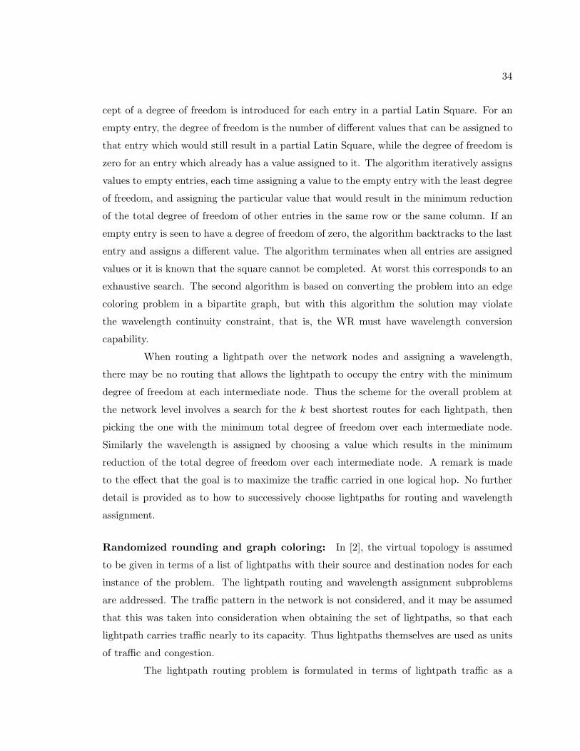
34
cept of a degree of freedom is introduced for each entry in a partial Latin Square. For an
empty entry, the degree of freedom is the number of different values that can be assigned to
that entry which would still result in a partial Latin Square, while the degree of freedom is
zero for an entry which already has a value assigned to it. The algorithm iteratively assigns
values to empty entries, each time assigning a value to the empty entry with the least degree
of freedom, and assigning the particular value that would result in the minimum reduction
of the total degree of freedom of other entries in the same row or the same column. If an
empty entry is seen to have a degree of freedom of zero, the algorithm backtracks to the last
entry and assigns a different value. The algorithm terminates when all entries are assigned
values or it is known that the square cannot be completed. At worst this corresponds to an
exhaustive search. The second algorithm is based on converting the problem into an edge
coloring problem in a bipartite graph, but with this algorithm the solution may violate
the wavelength continuity constraint, that is, the WR must have wavelength conversion
capability.
When routing a lightpath over the network nodes and assigning a wavelength,
there may be no routing that allows the lightpath to occupy the entry with the minimum
degree of freedom at each intermediate node. Thus the scheme for the overall problem at
the network level involves a search for the k best shortest routes for each lightpath, then
picking the one with the minimum total degree of freedom over each intermediate node.
Similarly the wavelength is assigned by choosing a value which results in the minimum
reduction of the total degree of freedom over each intermediate node. A remark is made
to the effect that the goal is to maximize the traffic carried in one logical hop. No further
detail is provided as to how to successively choose lightpaths for routing and wavelength
assignment.
Randomized rounding and graph coloring: In [2], the virtual topology is assumed
to be given in terms of a list of lightpaths with their source and destination nodes for each
instance of the problem. The lightpath routing and wavelength assignment subproblems
are addressed. The traffic pattern in the network is not considered, and it may be assumed
that this was taken into consideration when obtaining the set of lightpaths, so that each
lightpath carries traffic nearly to its capacity. Thus lightpaths themselves are used as units
of traffic and congestion.
The lightpath routing problem is formulated in terms of lightpath traffic as a

35
multicommodity flow problem which is known to be NP-complete. It is suggested that the
problem size can be reduced considerably by customizing the formulation for each instance
of the problem, in terms only of the lightpaths that are given, and also by pruning the
search tree by assuming that the optimal routing of a lightpath can always be found among
a few alternate shortest path routing of the lightpath on the physical topology. The integer
constraints of the formulation may also be relaxed.
The technique of randomized rounding is used as a heuristic algorithm to determine
lightpath routing. The goal is to minimize the number of wavelengths needed to establish
all the lightpaths. First, the integer constraint on the flows representing lightpaths are
relaxed, creating a non-integral multicommodity flow problem, and this is solved by some
linear programming method. Then, a phase called path stripping is carried out, in which
a set of possible paths is created for each lightpath. Successive paths for the commodity
representing that lightpath are found from among the links that carry any part of the flow
of that commodity in the solution to the relaxed flow problem. Each path is given a weight
equal to the minimum fraction of the commodity carried by a link in the path, and this
minimum value is subtracted from each link participating in the path. Once the set of paths
has been obtained for all the lightpaths, a single path is chosen for each lightpath randomly,
using the weights assigned during path stripping.
The wavelength assignment is presented as a separate subproblem once the light-
path routing has been carried out. A transformation of this problem to a graph coloring
problem which is known to be NP-complete is specified. An efficient well-known sequential
graph coloring algorithm called smallest-last coloring is specified as the chosen method due
to its simplicity.
The study employs known heuristic methods with provably good characteristics to
address the lightpath routing and wavelength assignment problems. It may be noted that
[2] demonstrates the use of the algorithms specified for dynamic as well as static lightpath
establishment.
Ring networks: The problem of designing logical topologies for rings that minimize
cost as measured by the amount of electro-optic equipment has recently received much
attention in the literature. Given the widespread use of SONET/SDH networks, it is not
surprising that some of the early work on WDM traffic grooming has focused on ring topolo-
gies [33, 6, 32, 30, 15, 16, 26, 21, 12]. In [26], the problem of wavelength assignment to

36
a given set of lightpaths is considered. The discussion focuses on how limited wavelength
conversion affects the capability of the network, and specific cases are discussed with con-
structive proofs. Several different virtual topologies for ring networks are discussed in [16]
in the light of the twin issues of traffic grooming and network cost, and characteristic met-
rics are derived. The study in [15] complements [16] by addressing only the wavelength
assignment issue, with the goal of minimizing the number of SONET ADMs. The concept
of lightpath splitting in designing a virtual topology is discussed and heuristics for wave-
length assignment are developed based on this concept. In [32], the problem of grooming
traffic is considered both for unidirectional and bidirectional rings, with a primary goal
of either minimizing the number of SONET ADMs or the number of wavelengths. The
strategy presented is to first construct circles from the given traffic components and then to
groom these circles. Algorithms for exact solutions for uniform traffic and heuristics for the
NP-hard non-uniform traffic case are presented. A similar approach of constructing circles
first is taken in [33], but now the resultant circles are scheduled in a sequence of virtual
topologies. Heuristic algorithms to minimize network cost by grooming are presented in [8],
for special traffic patterns such as uniform, certain cases of cross-traffic, and hub. In [6], the
concept of a t-allowable traffic pattern is discussed, in which the traffic for each node-pair is
constrained to be at most t. A bidirectional ring, but with symmetric traffic, is considered
for dynamic traffic. A heuristic algorithm based on a bipartite matching formulation of
the problem is presented, and blocking characteristics of the result are discussed. In [21],
a problem similar to that in [15] is considered, but the problem of routing the lightpaths
is considered as well as the wavelength assignment problem. An Euler-trail decomposition
of the ring network is presented, and a heuristic which uses one of the heuristics of [15]
and performs rerouting of lightpaths as well, based on the Euler-trail decomposition, is
presented. The characteristics of the architectures are discussed both for the case of limited
and unlimited number of available wavelengths. The studies [11, 32] note that the prob-
lem of logical topology design is NP-hard even for a physical ring topology, and obtaining
an exact solution requires significant amount of computation even for modest sized rings.
Heuristic approaches have been reported in literature [32, 33, 8, 15, 21].

37
3.2.3 Arbitrary Topologies
There are various studies proposing heuristic methods for arbitrary virtual topologies. These
studies address the virtual topology subproblem itself, as well as some or all of the sub-
sequent subproblems of virtual topology design. Most of these methods take into account
the effect of the network traffic pattern, since arbitrary virtual topologies are usually called
for in response to non-uniform traffic patterns and irregular physical topologies. Some of
the heuristics proposed are similar to each other. In this section we discuss such heuristic
approaches.
In [34], the problem is looked upon as the establishment of an optical connection
graph over a WAN based on the average traffic demand, and then using demand based
routing on this connection graph, that is, dynamic virtual circuits, which allocate whole
lightpaths at a time. The connection graph subproblem presented is therefore identical to
the first three subproblems of the virtual topology problem as presented in Section 2.2.2.
The problem is formulated as a nonlinear integer programming problem, and an approximate
decomposition is presented. The heuristic algorithm is then presented, which is based
on a greedy approach. The algorithm iteratively attempts to create as many lightpaths
as possible using each wavelength without violating the wavelength clash and continuity
constraints. Lightpaths are assigned between source-destination node pairs in descending
order of the amount of average traffic flowing between them, which favors one logical hop
traffic. By assigning a wavelength to as many lightpaths as possible before going on to
the next wavelength, the attempt is made to utilize the number of wavelengths used for a
maximum number of lightpaths. Only a predefined number of wavelengths can be used, and
the algorithm terminates when no more lightpaths can be set up using these wavelengths.
The authors remark that there is no guarantee that the virtual topology obtained would be
connected. To allow the routing of traffic from any node to any other on this topology, the
suggestion is made that the procedure be stopped when one wavelength still remains, and
then this wavelength be used to connect any disconnected subnetworks that may have been
formed before using it to form any other lightpaths that may be possible. The study goes on
to describe a routing scheme which dynamically allocates and deallocates these lightpaths
on demand, but this is outside the scope of this survey.
Several different heuristics are presented in [27]. The first one is simply called
“heuristic logical topology design algorithm”, and it also attempts to create lightpaths

38
between nodes in order of decreasing traffic demands. A network degree is assumed to be
given as part of the problem. Each lightpath is established between the nodes that have the
maximum amount of traffic between them which is not already carried by some lightpath,
provided wavelength clash, continuity, and degree constraints are obeyed. If all traffic is
accounted for but each node does not have the required degree, the rest of the lightpaths
are placed at random obeying the constraints. A modified version of this heuristic is also
presented which is only applicable if the logical degree is greater than the physical degree. In
this algorithm, a pair of lighpaths in opposite directions is initially set up for each physical
edge, then the original algorithm is exactly followed. This ensures that traffic can always
be routed on the shortest physical path between any two nodes and hence can satisfy any
physically realizable delay constraints. Another heuristic depends on the iterative bound
developed in this study by relaxing the MILP formulation as described in Section 3.1. The
higher values of the lightpath indicator variables are taken to represent actual lightpaths and
the lower values are discarded, obeying the degree constraints, yielding a virtual topology.
Finally, a heuristic is presented that does not take into account the traffic pattern at all,
but concentrates on creating lightpaths that use only a few physical edges, since this should
conserve wavelengths. Thus the heuristic first creates lightpaths between all nodes which
are one physical hop apart, then between all nodes which are two physical hops apart, and
so on, while the degree constraints are not violated. Wavelength assignment algorithms
for the last two heuristics are not discussed, and lightpath routing for the LP relaxation
algorithm is not discussed.
A similar heuristic maximizing one logical hop traffic is briefly described in [3], but
a heuristic with the opposite objective is also suggested. Since in a virtual topology some
traffic will always be carried in multiple logical hops because of constraints on number of
wavelengths and node degrees, a heuristic approach must account for multihop traffic and
not only concentrate on maximizing single hop traffic. Accordingly, this heuristic aims at
maximizing multihop traffic. Some results are provided in which the two approaches appear
to perform very similarly to each other. Details of wavelength assignment are not discussed.
The study in [4] also suggests that attempts to maximize one logical hop traffic
concentrates on the comparatively larger traffic components, and may cause the smaller
traffic components to be routed unreasonably and cause congestion on some physical links.
A scheme is presented to avoid this. A complete bipartite graph is created in which each
partition contains all nodes of the physical topology. The edges are weighted with traffic

39
demands between corresponding nodes. Each edge represents the shortest physical path
between corresponding nodes. Now a minimum weighted perfect matching is identified and
the corresponding edges are eliminated from this graph. The traffic carried by the eliminated
edges is rerouted over the least congested of the remaining edges. This is repeated until
the number of edges connected to each node has been reduced from N to ∆l, the desired
logical degree. Now this graph represents a logical topology with each edge representing a
lightpath. The lightpath routing and wavelength assignment can be done arbitrarily and
the congestion will be the same, but different number of wavelengths will be required. Since
minimizing the number of wavelengths is known to be NP-hard, a known path-graph based
algorithm is specified for path embedding and wavelength assignment. This algorithm
is described in literature referred to in [4]. If the number of wavelengths is more than
the number desired, extra wavelengths may be eliminated by choosing wavelengths which
implement the least number of lightpaths, and rerouting traffic carried by those lightpaths
along others with least load.
In [19], a heuristic algorithm following the LP relaxation heuristic from [27], but
more complete, is presented. After rounding the lightpath indicator variables obtained by
a suitable number of iterations of the LP obtained by relaxing the exact formulation, the
virtual topology subproblem has been solved. The constraint on the number of physical
hops for lightpaths, which is a part of the exact formulation provided in [19], may be lost
in the relaxation, in the sense that some lightpaths may be formed with larger number
of hops than was allowed for in the exact formulation. Now the lightpath wavelength
indicator variables are also rounded using a specified rounding algorithm which sets the
highest of the alternative values to 1 and the rest to 0, maintaining consistency with the
lightpath indicators as rounded previously. This results in a set of lightpath routings for
each lightpath. Then a path of least resistance is followed for each lighpath from among the
possible choice of paths to pick the routing for the lightpath. It appears that backtracking
may be necessary at this stage. At the end of this stage, a tentative wavelength assignment is
also obtained, but this assignment may not be free of clash. The last stage of the procedure
is to resolve wavelength clashes. Different approaches to this are discussed in [19], and
the one specified involves coloring a path-graph by first listing nodes in order of decreasing
degree, removing one node each time, and then sequentially assigning the first available free
color to the nodes in this order. A remark is made that the results obtained using the other
approaches specified are similar. This results in a wavelength assignment on the original

40
virtual topology. It appears that the bound on the number of wavelengths, which is part of
the exact formulation provided, may not be strictly obeyed by the final solution obtained
by following this procedure.
3.3 Related Approaches
In this section we discuss some techniques and algorithms that are different from those
described in Section 3.2, but which are related to the problem of virtual topology design
for wavelength routed networks.
Incremental Benefit Analysis: In [25], a study of the incremental benefits of introduc-
ing a virtual topology over optical WANs is undertaken. Several simplifying assumptions
such as infinite buffers and adequate number of wavelengths is made. The authors obtained
data regarding the traffic pattern in the T1 NSFNET backbone network. The data was col-
lected in January 1992. At that time, the NSFNET backbone used optical fibers as physical
medium, but only as T1 links, without the use of either WDM or wavelength routing. This
data serves to establish the pattern of traffic only, that is, the proportion of total traffic in
the network flowing between each source-destination node pair.
The goal of implementing techniques such as WDM or virtual topologies in such
a network would be to scale up this traffic pattern. Thus we would like to increase the
overall traffic flowing in the network without changing the relative quantities of different
source-destination traffic. This is the equivalent of designing a virtual topology for minimum
congestion as we discussed before. The pattern is scaled up in three different ways. First,
the method of flow deviation is used to scale up the traffic pattern without the use of
either WDM or wavelength routing, but merely by routing traffic efficiently. This serves as
the baseline with which to compare scaleup benefits obtained with the use of the other two
techniques. A maximum scaleup factor of 49 was observed. This scheme uses two lightpaths
in each direction corresponding to each fiber, and is thus equivalent to a virtual topology
which is the same as the physical topology, with a single wavelength.
The second scheme uses WDM, but no wavelength routing. In other words, each
fiber now acts as not one but multiple point-to-point lightpaths, but there are no lightpaths
spanning multiple physical links. The nodal degree was limited to 4 and lightpaths were
added by inspection. The best scaleup factor was now observed to be 57.

41
The last scheme applies wavelength routing as well as WDM, to implement arbi-
trary lightpaths and virtual topologies, though it appears that the virtual topologies are all
chosen to be hypercubes. Simulated annealing as discussed previously in [25] was applied to
find the best possible virtual topologies in terms of scaleup. The maximum scaleup factor
was observed to be 106.
It was noted that the average packet delay, as well as propagation delay and
queueing delay, both of which were modeled, increased somewhat over the three schemes.
However, the average number of logical hops decreased. The most dramatic result is in the
increase of the scaleup factor, and the link utilization which went from 32% and 23% in the
minimum loaded link in the first two schemes to 71% in the last one, while the maximum
link load remained 99% in all three schemes. Thus this analysis provides demonstration of
the benefits of implementing a virtual topology, as well as the incremental nature in which
it may be undertaken.
Limited Conversion: The motivation for the study presented in [26] is the lower cost
associated with limited conversion of wavelengths at Wavelength Routers as opposed to full
conversion, as we remarked in Section 2.1. In this study, some terms related to limited
conversion are first defined. Theoretical results are derived regarding the virtual topologies
which networks with limited conversions can support. A network node is said to have a
wavelength degree k if each wavelength at an input port can be switched to one of a
maximum of k wavelengths at the output port. Not all wavelengths may be switchable
to k different wavelengths. In terms of our earlier terminology, full wavelength conversion
would correspond to a wavelength degree of W , with every wavelength switchable to every
other, and fixed and no wavelength conversions would both be represented by a wavelength
degree of 1. The set of lightpaths to be established, in terms of their source and destination
nodes, as well as the route to be followed, are assumed to be given. Thus the wavelength
assignment subproblem is the focus of this study. Several results are obtained in theoretical
terms about ring networks with specific wavelength conversion capabilities. For example,
it is shown that a ring network with full wavelength conversion capability at one node and
no wavelength conversion at the others can be used to assign clash free wavelengths to any
set of lightpaths, as long as the maximum number of lightpaths assigned a path over a
single physical link is no more than W (which is a physical bound). A similar result is also
derived with a ring network that has two nodes of wavelength degree 2, and no wavelength

42
conversion at the others. All these results are followed by constructive proofs rather than
simply existence proofs, so that a blueprint is provided for the actual construction of such
ring networks.
Similar results are derived for more general physical network topologies. In partic-
ular, results are derived about a star network where limited wavelength conversion is only
employed at the single hub node. There is a corollary which can be used to extend this
result to arbitrary topologies, with the (somewhat severe but not entirely unreasonable) re-
striction that the number of physical hops is no more than 2 for any lightpath in the virtual
topology. A result removing this restriction for the case of physical topologies in the form
of specially constructed tree networks is stated but no constructive proof is supplied. It is
stated that a proof is possible, but it is not mentioned whether the proof is constructive.
All the results in this study are exact and none depend on heuristic methods. It
is not entirely clear how to integrate this with heuristic techniques which can solve other
subproblems, or how to extend this work to arbitrary topologies, but the issue of limited
wavelength conversion capabilities would appear to be worth further investigation.
Generalized Lightpaths: In [29], the concept of a lightpath is generalized into that of
a lighttree, which, like a lightpath, is a clear channel implemented with a single wavelength
with a given source node. But unlike the lightpath, a lighttree has multiple destination
nodes, thus a lighttree is a point-to-multipoint channel. The physical links implementing
a lighttree form a tree rather than a path in the physical topology, hence the name. The
points that are emphasized in this study are the following. A lighttree is a more general
representation of a lightpath, hence the set of virtual topologies that can be implemented
using lighttrees is a superset of the virtual topologies that can be implemented only using
lightpaths. Thus for any given virtual topology problem, an optimal solution using lighttrees
is guaranteed to be at least as good and possibly an improvement over the optimal solution
obtained using only lightpaths. Another attractive feature of lighttrees is the inherent
capability for optical multicasting. The current study refers to only unicast and broadcast
traffic problems and identifies the multicast problem as an area of ongoing study. An
illustrative example is given, and the mathematical formulation of the problem is outlined.
Optical switch architectures involved in networks based on lighttrees is also reviewed.
As pointed out previously, the optimal solution using a more general construct
is certain to improve on the optimal solution with a less general one. However, as we

43
already know, optimal solutions are not practically obtainable, and with a more general
construct and hence a much larger search space this is going to be even more true. Heuristic
solutions will have to be designed to obtain good solutions, and must be tailored to suit the
larger search space. With unicast traffic problems, the lighttree approach trades off more
bandwidth to further improve delay, congestion, and physical hop characteristics than the
lightpath approach. This is the tradeoff we mentioned in Chapter 1. The challenge in this
case will be to design heuristics that can cope with the increased complexity of the problem
and yet produce solutions in which a good tradeoff is achieved. This appears to be an area
worth further investigation.
3.4 Reconfigurability Considerations
Since the virtual topology problem is defined on a static traffic matrix, the topology must
be redesigned when the aggregate traffic pattern changes significantly. Thus the problem of
reconfiguring a network from one virtual topology to another is a related problem to virtual
topology design. Two possible approaches to this problem are discussed in this section.
3.4.1 Cost Approach
In this approach, it is assumed that the current virtual topology as well as the new virtual
topology that the network must be reconfigured to are known, together with the physical
topology details. The concern is to minimize the cost of the reconfiguration. The cost can
be expressed in terms of the number of Wavelength Routers that need to have their optical
switching reprogrammed, or the total number of optical switchings that need to be changed
to implement the new lightpaths and eliminate old ones. These metrics are appropriate since
they reflect the amount of time the network must be taken off line to make the changes,
as well as the reprogramming effort for the reconfiguration. Other similar metrics may
also be applicable. It may be the case that the network cannot be taken off line at all,
but that a succession of intermediate virtual topologies have to be designed to eliminate
single, or groups of, routers which can be reconfigured and put back in operation. Much
more complicated metrics reflecting total time taken to reconfigure as well as the effort to
redesign the intermediate topologies need to be developed in this case.
We have not found any study of these reconfiguration problems in the literature for
wavelength routed WANs, though studies involving the reconfiguration of virtual topologies

44
for broadcast LANs exist, as detailed in the survey of related literature carried out in [20].
These studies involve link-exchange and branch-exchange techniques to minimize the cost
of converting one virtual topology into another, and similar methods may be possible to
exploit for the wavelength routed wide area network.
3.4.2 Optimization Approach
Another approach is to assume that only the current virtual topology is given, together with
the changed traffic pattern and/or physical topology that makes reconfiguration necessary.
This is the approach taken in [3]. The reconfiguration algorithm proposed in [3] involves
solving the new virtual topology problem on its own without reference to the current virtual
topology to obtain a new optimal solution, with a new optimal value for the objective
function which is noted. The virtual topology design problem is then reformulated with
an additional constraint that constrains the old objective function to this noted value, and
a new objective function that involves minimizing the number of lightpaths that must be
either added or removed.
While this method is guaranteed to find a solution that results in a virtual topology
that is optimal for the new conditions, it does not achieve a balance between finding an
optimal new virtual topology and one that involves as little change from the old one as
possible. It is possible that a very costly reconfiguration will be undertaken for only a slight
gain in network performance. More balanced formulations of this problem may be possible,
and heuristics designed on such formulations are likely to perform better in practice.

45
Chapter 4
Ring Networks
In this chapter, we consider networks with the physical topology of a unidirectional
ring. As has been noted in literature [11, 32], the problem of logical topology design is NP-
hard even for a physical ring topology, and obtaining an exact solution requires significant
amount of computation even for modest sized rings. Heuristic approaches are needed for
practical purposes and have been reported in literature [32, 33, 8, 15, 21]. To evaluate
the performance of such heuristic approaches when the optimal solution is not available,
achievability bounds are useful.
The problem of interest is to groom lower speed traffic streams into the wavelengths
available, that is minimize electronic routing of traffic. In this context, we have created a
framework of bounds, both upper and lower, on the optimal value of the amount of traffic
electronically routed in the network.
The bounds are obtained based on the idea of decomposing the ring network a
few nodes at a time. We specify the decomposition method and derive a result showing
that solving the decompositions is a considerably more tractable problem than solving the
complete problem. We present a method of combining these partial solutions into a sequence
of bounds, both upper and lower, in which every successive bound is at least as strong as
the last one. We derive a result showing how close the final upper and lower bounds are
guaranteed to be to each other. An algorithm is developed which enables us to combine the
decompositions into bounds without facing a combinatorial explosion.
We present numerical results of the computation of these bounds by computing
the bounds on different families of traffic matrices. For small rings, we can compute nearly
all the bounds in the framework. Numerical results indicate that in these cases the expec-

46
tations from theoretical considerations are fulfilled. For larger rings, the sequence cannot
be computed to the end and we are limited by the availability of computing power in how
far we can compute this sequence. The numerical results show that we can get good results
in either case.
The framework can be adapted to other formulations of the problem on the ring
network, such as bidirectional rings or quantized objective functions. The bounds help
us in evaluating heuristics which must be used in practical situations because of the NP-
hard nature of the problem. The upper bounds are based on constructing actual feasible
topologies on the network, and thus also provide us with a sequence of increasingly good
heuristics. Thus, we feel this is a useful framework in a broad context of ring problems for
wavelength routing optical networks.
4.1 Problem Formulation
We consider a unidirectional ring R with N nodes 1, numbered from 0 to N − 1, as shown
in Figure 4.1(a). The fiber link between each pair of nodes can support W wavelengths,
and carries traffic in the clockwise direction; in other words, data flows from a node i to
the next node i⊕ 1 on the ring, where ⊕ denotes addition modulo-N . (Similarly we use �to denote subtraction modulo-N .) The links of R are numbered from 0 to N − 1, such that
the link from node i to node i⊕ 1 is numbered i. Each node in the ring is equipped with a
WADM. We focus on the detail of the connection of a WADM to the network in the context
of traffic grooming (see Figure 4.1(b)). A WADM can perform three functions. It can
optically switch some wavelengths from the incoming link of a node directly to its outgoing
link without the need for electro-optic conversion of the signal carried on the wavelength.
It can also terminate (drop) some wavelengths from the incoming link to the node; the
data carried by the dropped wavelengths is converted to electronic form and undergoes
buffering, processing, and possibly, electronic switching at the node. Finally, the WADM
can also add some wavelengths to the outgoing link; these wavelengths may carry traffic
originating at the node, or they may carry traffic originating at previous nodes in the ring
and electronically switched at this node.
The important point to note is that ordinary LTE’s such as SONET ADM’s are1We describe the working part of the ring. It is assumed that there is a protection part for self-healing
or fault-tolerance as dictated by design or required by standards, but our description does not include this.

47
01
(a)
i
i-1 i+1
...
N-1
..
.
from i-1
(b)
i
to i+1
Figure 4.1: (a) An N -node unidirectional ring, and (b) detail of a node with a WADM
required for each wavelength that is dropped/added at a WADM, but not for a wavelength
that is passed through. Since the traffic contained in the dropped wavelengths must be
electronically processed at very high speeds, these LTE’s are very costly equipment.
As before, the traffic demands between pairs of nodes in the ring are given in the
traffic matrix T = [t(sd)], each quantity t(sd) ∈ {0, 1, 2, · · ·} expressed in terms of the basic
rate. We let C denote the capacity of each wavelength expressed in units of this basic rate.
Given the ring physical topology, a logical topology is defined by establishing light-
paths between pairs of nodes. A lightpath is a direct optical connection on a certain wave-
length. More specifically, if a lightpath spans more than one physical link in the ring, its
wavelength is optically passed through by WADMs at intermediate nodes, thus, the traffic
streams carried by the lightpath travel in optical form throughout the path between the
endpoints of the lightpath. We assume that ring nodes are not equipped with wavelength
converters, therefore a lightpath must be assigned the same wavelength on all physical links
along its path.
An important problem that has received considerable attention in the literature is
the design of logical topologies that optimize a certain performance metric. The performance
metric of interest in this work is the amount of electronic forwarding (routing) of traffic
streams, since such forwarding involves electro-optic conversion and added message delay
and processor load at the intermediate nodes. There is also the possibility of increased buffer
48
requirement and queueing delay. In a global sense, this means that we want to reduce the
number of logical hops taken by traffic components, individually or as a whole. For each
node, it also means that we want to reduce the amount of traffic that node has to store and
forward. Thus we have two alternative goals, one is to minimize the total traffic weighted
logical hops in the network, and the other is to minimize the maximum number of traffic
components electronically routed at a node. In this paper we have chosen to concentrate
on the former. A single traffic unit may not be bifurcated, but different traffic units for
the same source-destination traffic component are looked upon as separate traffic and may
be assigned different logical routes. Another possible quantity of interest is the number of
wavelengths each WADM is required to add or drop due to lightpath terminations. This
would correspond to the minimizing of the number of SONET ADM’s as in [32, 8, 15, 21]. It
should be noted that adding and dropping more wavelengths will result in a larger number
of logical hops for traffic components and thus this concern is to some extent incorporated
in the electronic forwarding issue we mentioned above.
We let t(l) denote the aggregate traffic load on the physical link l (from node l to
node l ⊕ 1) of the ring. The value of t(l) can be easily computed from the traffic matrix
T by adding up all traffic components t(sd) such that the path from s to d includes the
physical link l (note that, because of our assumption of unidirectional traffic flow around
the ring, there is exactly one path between any pair of nodes). The component of the
traffic load t(l) due to the traffic from source node s to destination node d is denoted by
t(sd)(l). If one or more lightpaths exist from node i to node j in the virtual topology, the
traffic carried by those lightpaths is denoted by tij . The component of this load due to
traffic from source node s to destination node d is denoted by t(sd)ij . In our formulation, we
forbid a traffic component to be carried completely around the ring before being delivered
at the destination, thus each traffic component can traverse a given link at most once.
This is reasonable because carrying the traffic component around the ring consumes more
bandwidth, and is likely to require more logical hops.
In our formulation we allow for multiple lightpaths with the same source and
destination nodes. We denote the lightpath count from node i to node j by bij , taking its
value from {0, 1, 2, · · · ,W}. We also define the potential lightpath set for a link to be the
set of lightpaths that would pass through a given link, and denote it by B(l) = { (i, j) |lightpath (i, j), if it existed, would pass through link l }.
With the above notation, we can now formulate the problem of designing a virtual

49
topology for a ring network such that the total amount of electronic routing at the ring
nodes is minimized. The following formulation as an Integer Linear Problem (ILP) consists
of O(N4+N2W ) constraints and O(N4+N2W ) variables, where N is the number of nodes in
the ring, and W the number of wavelengths. It follows the general formulation we provided
in Section2.2.1, other than the enhancements mentioned above. In addition, the lightpath
routing variables and constraints are missing, since the lightpath routing subproblem is
effectively eliminated in the unidirectional ring topology: only a unique physical route is
available to a lightpath with a given source and destination.
Given:
The physical topology, a unidirectional ring R of N nodes
The traffic matrix T = [t(sd)], s, d ∈ {0 · · · (N − 1)}t(sd) ∈ {0, 1, 2, · · ·}t(ss) = 0,∀s
The wavelength limit W which is the number of distinct wavelengths each fiber link
can carry.
Find:
Virtual topology, in terms of lightpath indicators bij , lightpath wavelength indicators
c(k)ij , and the traffic routing variables t
(sd)ij .
Subject to:
Traffic Constraints
t(sd)ij ≤ t(sd)(i), ∀(i, j), (s, d) (4.1)
t(sd)ij ∈ {0, 1, 2, · · ·}, ∀(i, j) (4.2)∑
(i,j)∈B(l)
t(sd)ij = t(sd)(l), ∀(s, d), l (4.3)
tij =∑
sd t(sd)ij , ∀(i, j) (4.4)
tij ≤ bijC, ∀(i, j) (4.5)

50
∑j
t(sd)ij −
∑j
t(sd)ji =
t(sd), s = i
−t(sd), d = i
0, s �= i, d �= i
∀i, (s, d) (4.6)
Wavelength Constraints
∑(i,j)∈B(l)
bij ≤ W, ∀l (4.7)
∑k
c(k)ij = bij , ∀(i, j) (4.8)
∑(i,j)∈B(l)
c(k)ij ≤ 1, ∀l, k (4.9)
To minimize:
min
∑
s,d,i,j∈{0···(N−1)}t(sd)ij −
∑s,d∈{0···(N−1)}
t(sd)
(4.10)
In the above, the traffic constraint (4.1) ensures that a lightpath can carry traffic
for a source-destination node pair only if it is in the physical route of the traffic component.
Constraint (4.3) states that the physical traffic on a link due to a source-destination node
pair must be equal to the sum of the traffic on all lightpaths passing through that link
due to that node pair. Constraints (4.4, 4.5) define the total traffic on a lightpath and
relate it to the lightpath count, respectively. Because of the definition of the quantities
t(sd)(l), the constraints (4.1, 4.3) together ensure that no traffic component can be routed
completely around the ring before being delivered at the destination node. Constraint (4.6)
is an expression of traffic flow conservation at lightpath endpoints. Among the wavelength
constraints, constraint (4.7) expresses the bound imposed by number of wavelengths avail-
able, (4.8) relates the wavelength indicators to the lightpath counts, and (4.9) ensures that
no wavelength clash can occur.
The framework we present below is based on the above formulation we have cho-
sen, but this formulation is not essential for it. The framework can be adapted to many
variations that are possible in the formulation. There may be multiple fiber links be-
tween successive nodes, and the nodes may be equipped with wavelength routers instead
of WADMs. Hardware for wavelength conversion, limited or otherwise, may be available
at the nodes [26]. A physical hop limit for lightpaths may be imposed on feasible topolo-
gies, due to physical fiber characteristics or OAM issues. The ring may be bidirectional,

51
either with some simple routing strategy (such as shortest-path, as in [32, 15]) that allows
us to consider it as two unidirectional rings, or the lightpath routing (either clockwise or
counter-clockwise) may be integrated as part of the optimization process (as in [21]). In all
these cases, the grooming objective may be to minimize electronic routing. The framework
we present may be extended, in a straightforward manner for some of these cases, and with
some enhancements in others. When the objective is not an additive function as in our
formulation but some other function such as a min-max type (minimize electronic routing
at the node with maximum electronic routing) or a quantified version (minimize number of
wavelengths added/dropped, number of SONET ADMs, etc.) our framework can also be
adapted to obtain bounds for the optimal value of the objective function.
4.2 Path Decomposition of a Ring Network
4.2.1 Definition of Decomposition
We consider a ring R with N nodes labeled 0 · · · (N − 1), in order, and traffic matrix T .
We define a segment of length n, 1 ≤ n ≤ N , starting at node i, 0 ≤ i < N , as the part of
the ring R that includes the n consecutive nodes i, i⊕ 1, i⊕ 2, · · · , i⊕ (n− 1), and the links
between them.
We define a decomposition of ring R around a segment of length n starting at node
i as a path P(i)n that consists of n + 2 nodes and n + 1 links as follows: the n nodes and
n − 1 links of the segment of ring R of length n starting at node i, a new node S and a
link from S to i, and a new node D and a link from node i ⊕ (n − 1) to D. We also refer
to P(i)n as an n-node decomposition of ring R starting at node i. Figure 4.2 shows such a
decomposition.
Associated with the decomposition P(i)n is a new traffic matrix TP(i)
n=
[t(sd)
P(i)n
],
s, d ∈ {i, i⊕ 1, · · · , i⊕ (n− 1), D, S}, derived from T , the original traffic matrix, as follows:

52
01
i-1
i
i+1
N-1
i+n-1
i+n
(a)
...
....
.. .
i
i+1
i+n-1
S D
(b)
. ..
Figure 4.2: An n-node decomposition: (a) original ring R with N nodes, and (b) a decom-
position P(i)n of the ring around a segment of length n starting at node i
t(sd)
P(i)n
=
t(sd), if i � s ≺ d � i⊕ (n− 1)∑j /∈{i,i⊕1,···,d�1} t
(jd), if s = S, i � d � i⊕ (n− 1)∑j /∈{s⊕1,s⊕2,···,i⊕(n−1)} t
(sj), if d = D, i � s � i⊕ (n− 1)
tpass−thru(i, n), if s = S, d = D
0, if
s = d or
s = D or
d = S or
i � d ≺ s � i⊕ (n− 1)(4.11)
where tpass−thru(i, n) denotes the traffic of the original matrix T that passes through the
segment of length n starting at node i, i.e., traffic on ring R that uses the links of the
segment but does not either originate or terminate at any of the nodes in that segment.
We call this the pass-through traffic. The amount of this traffic can be readily obtained by
inspection of traffic matrix T . We have used s ≺ d in the above expression to denote that
node s precedes node d in the decomposition and s � d to denote that node s precedes and
may be the same as node d in the decomposition.
The traffic matrix for the decomposition is defined such that the traffic flowing

53
from a node s to another node d, such that s ≺ d, in the segment is the same as that in the
original ring for the corresponding nodes (see the first expression in (4.11)). Thus any traffic
component the path of which is entirely in the segment is unchanged in the decomposition.
The decomposition is effected by the introduction of the two nodes S and D together with
the links connecting them to the segment. In the decomposed network, node S acts as the
source of all traffic components in the original matrix T originated at a node outside the
segment and destined to any node in the segment (refer to the second expression in (4.11)).
Node S also acts as the source for all traffic components that pass through the segment, as
the fourth expression in (4.11) indicates. Similarly, node D is the sink for traffic originating
at any node in the segment and terminating at a node outside the segment in the original
ring (see the third expression in (4.11)), as well as for pass-through traffic. Finally, any
traffic components in the original matrix T that do not originate or terminate at nodes of
the segment, or do not traverse any links of the segment, are not included in the traffic
matrix for the decomposition. This is captured by the last expression in (4.11) where it is
shown that no traffic flows from node D to node S in the decomposition.
Because of the way the traffic matrix for the decomposition is defined in (4.11),
from the point of view of any node k, i � k � i⊕ (n− 1) in the segment, the traffic pattern
in the new path P(i)n is exactly the same as in the original ring. The new nodes S and
D are introduced in the decomposition to abstract the interaction of traffic components
between nodes in and outside the segment. Specifically, the new node S hides the details
of how traffic sourced at ring nodes outside the segment and using the links in the segment
actually flows over the rest of the ring, by providing a single aggregation point for this
traffic. Similarly, the new node D provides a single aggregation point for traffic using the
links of the segment and destined to nodes outside the segment, hiding the details of how
this traffic flows in the rest of the ring. Finally, the fact that P(i)n is a path (i.e., that there
is no link from node D to node S) means that the details of traffic in the original ring that
does not involve any nodes or links of the segment are hidden in the decomposition.
4.2.2 Solving Path Segments in Isolation
Consider the traffic matrix TP(i)n
=[t(sd)
P(i)n
]of the decomposition P(i)
n of a segment of length
n starting at node i in the ring R, as given in (4.11). This matrix can be thought of as
representing the traffic demands in a ring network consisting of nodes S, i, . . . , i⊕(n−1), D,

54
0 n-11 2 n-2
Figure 4.3: A unidirectional n-node path network
where there is simply no traffic flowing over the link from node D to node S. Consequently,
the ILP formulation we presented in Section 4.1 can be used to obtain a virtual topology
that minimizes electronic routing for this ring with traffic matrix TP(i)n
. Since the ILP
formulation disallows traffic routing that carries a traffic component beyond its destination
and all around the ring, no lightpaths can be formed to carry traffic over the link from D
to S that is absent in the decomposition. Thus, the topology obtained in this manner can
be directly applied to the path P(i)n . When we use the ILP to find an optimal topology for
path P(i)n we will say that we solve the n-node segment in isolation.
The topology obtained by solving an n-node segment in isolation does not take
into account the details of the original ring outside of the n-node segment. Such a topology
will only be optimal with respect to this n-node segment, in the sense that it will minimize
the amount of electronic routing within the segment, but without considering the effects
that doing so would have on the amount of electronic routing at nodes of ring R outside
the segment. In fact, this topology may not be optimal for the ring as a whole. In other
words, it is possible that, for any optimal topology for the ring as a whole, the subtopology
corresponding to the n-node segment will be different than the topology obtained by solving
the ILP for P(i)n in isolation. Thus it may not be possible to combine optimal solutions to
different segments in isolation into a (near-)optimal topology for the original ring R. Our
contribution is in proving a looser result: that it is possible to combine optimal solutions
to different segments in isolation to obtain lower and upper bounds on the optimal solution
to the ring R as a whole.
Our motivation for using the path decomposition described in this section is two-
fold. First, as the number n of nodes in a segment starting at some node i increases, the
resulting decomposition P(i)n will more closely approximate the original ring. As a result, the
bounds we obtain will be tighter with increasing n. Second and more importantly, a path
decomposition significantly alleviates the problem of exponential growth in computational

55
requirements for solving the original ILP for an n-node network. This result is a direct
consequence of the following lemma.
Lemma 4.2.1 A wavelength assignment always exists for a feasible virtual topology on a
unidirectional path network, and it can be obtained in time linear in the number of links
and the number of wavelengths W per link.
Proof. Consider a path network with n nodes as shown in Figure 4.3. Consider any feasible
virtual topology on this network, that is any topology for which the number of lightpaths
crossing any link is no more than W . If there is any link with less than W lightpaths,
we add as many single hop lightpaths on that link as necessary to make the number of
lightpaths on that link equal to W . Now we can assign wavelengths to all the lightpaths in
a straightforward manner. At the first link from node 0 to node 1, we have W lightpaths
to which we can assign W wavelengths in any arbitrary fashion. We then examine these
lightpaths in some particular order. Consider a lightpath assigned wavelength w on the first
link from node 0 to node 1. If the lightpath continues onto the second link from node 1 to
node 2, we assign the wavelength w to this lightpath on the second link. If the lightpath
terminates at node 1, we know that another lightpath originates at node 1, since the load
on each link is the same. We pick one such lightpath, breaking ties arbitrarily, and assign
it wavelength w. We continue in this manner, assigning wavelengths to the lightpaths on
each link until we reach the last node and have colored all the lightpaths. We are guaran-
teed to be able to reach node n − 1 on each of the W wavelengths, because no lightpath
passes through or originates at node n − 1. Now we have assigned a wavelength to all the
original lightpaths of the feasible virtual topology we started with and can discard the sin-
gle hop lightpaths (if any) that were added to bring the number of lightpaths at each link
to W . Since all feasible topologies have a wavelength assignment so does the optimal one.
In solving the decomposed problem, we are merely interested in the optimum value
of the objective, since this is the value from which we will obtain the bounds. Since we
know that a wavelength assignment is always possible and we are not interested in the
details of the wavelength assignment, we can eliminate the wavelength assignment from
our formulation altogether. This implies that we can eliminate the wavelength assignment
subproblem from the list of subproblems we enumerated in Section 2.2.2. Thus, we eliminate
the wavelength variables c(k)ij and the constraints (4.8) and (4.9). The number of variables
56
in the formulation remains O(N4), but N2W variables are eliminated, and the number
of wavelength constraints is reduced from O(N2W ) to O(N), though the total number
of constraints remains O(N4). This creates a formulation that is smaller and requires
dramatically less computation to solve. In practice, we have found that eliminating the
wavelength assignment subproblem can result in a reduction in computation time by several
orders of magnitude. For instance, completely solving a six-node ring network using the
original formulation (with wavelength assignment) requires between 60 and 90 minutes on
a Sun Ultra-10 workstation. However, solving a six-node path network using the simplified
formulation (no wavelength assignment) requires only a few seconds. In both cases, we used
the LINGO scientific computation package which utilizes branch-and-bound algorithms to
solve the ILP.
A further improvement to the ILP formulation that reduces the running time for
path networks may be obtained by explicitly forbidding any lightpaths that traverse the
link from D to S, that is, by fixing the values of some lightpath counts to zero:
bij = 0, ∀ bij ∈ B(D,S) (4.12)
where i, j refer to nodes in the decomposition.
We have devised a way to further reduce the computational efforts required to solve
the ILP for a path segment; the tradeoff is an increase in the complexity of the formulation.
In this approach, we customize the formulation to include information about combinations
of lightpath variables that can produce feasible solutions, eliminating combinations we know
are not consistent by application of problem-specific logic. We can also prune the search
space by a large factor by creating a space that we know contains exactly one optimal
solution. The formulation has to be customized for each value of n, where n is the number
of nodes in the decomposed segment. The amount of logic and extra information to be
included in such a custom formulation increases rapidly with n. We have carried out such
customizations for 2- and 3-node decompositions (the case for a single-node decomposition is
trivial). The gain in computational effort appears to be more than offset by the complexity
of the formulation beyond this point, and as such, this method was not carried out any
further.

57
4.2.3 Interpretation of the Optimal Value for Decomposed Paths
We denote the optimal objective value for the decomposition P(i)n by φ
(i)n . That is, φ(i)
n is the
amount of electronic routing performed by the optimal virtual topology on the decomposi-
tion P(i)n . In the decomposition, n of the n + 2 nodes which are the same as in the original
ring see the same traffic pattern locally as they do in the original ring, as we remarked above.
The two additional nodes S and D, by the construction of the decomposition, do not have
any traffic passing through them at all, and hence they do not contribute any electronic
routing in any feasible virtual topology on the decomposition. Thus, the optimal objective
value φ(i)n for the decomposition P(i)
n is contributed only by the n nodes abstracted from the
ring. Since the traffic pattern seen by these nodes is the same as when they are included in
the ring, φ(i)n also represents the locally best (lowest) amount of electronic routing at this set
of nodes when considered as part of the ring. In other words, the electronic routing at this
set of nodes is minimized, irrespective of how much electronic routing has to be performed
at other nodes of the original ring as a result.
It might appear that as we include more and more nodes in the decomposition,
the optimal solution to the original problem will be obtained when all N nodes have been
represented in the decomposed network (that is, when we have a decomposition consisting
of N + 2 nodes). However, because we convert the ring to a path, some information is not
taken into account at the point where we “open up” the ring when considering an N node
decomposed network. As a result, solving an N -node decomposition does not provide the
optimal solution for the N -node ring. This is clear from arguments related to this topic in
[26, 21], for convenience we present the argument in the current context here. Consider the
decomposition of an N -node segment starting at node i. Now note that the decomposed
path P(i)N contains all nodes and links of the original ring except the link from node i� 1 to
node i; this is where the ring is “opened up” to introduce the new nodes S and D. Consider
a lightpath in the original ring that originates at a node s ≺ i�1 and terminates at a node d
such that i ≺ d, and therefore uses the link i�1 (from node i�1 to node i) in the ring. Any
such lightpath will be represented by two lightpaths in the decomposition P(i)N : one from
the new node S to node d, and one from the new node D to node s. Since these lightpaths
are not constrained to use the same wavelength in the decomposed network, a wavelength
assignment for the N -node decomposition may not be feasible for the N -node ring. Thus,
the optimal solution to the decomposition may not be possible to translate to a solution

58
0
(a)
.
S D
(b)
ii+1i-1
1 N-1
.
i
..
..
.
Figure 4.4: A single node decomposition of a ring: (a) original ring, and (b) single node
decomposition P(i)1 around node i
to the original ring, and we still have an optimal value φ(i)N for the N -node decomposition,
rather than an optimal value for the ring R.
4.3 Bounds
In this section we describe how we can combine the φ(i)n values we get from n-node decom-
positions to obtain lower as well as upper bounds on the total amount of electronic routing
performed in the optimal case by a virtual topology on the original ring. The method of
combination is different for lower and upper bounds. We first discuss the case where we
only consider single-node decompositions, then move on to the general case where larger
decompositions are available.
4.3.1 Bounds Based on Single-Node Decompositions
A decomposition of an N -node ring around a single node i is shown in Figure 4.4. The next
two sections show how to obtain lower and upper bounds, respectively, on the optimal ILP
solution for the ring as a whole by appropriately combining the optimal ILP solutions φ(i)1
for the possible single-node decompositions P(i)1 , i = 0, · · · , (N − 1).

59
Lower Bound
Recall that φ(i)n represents the locally best amount of electronic routing at the nodes in the
segment of length n starting at node i. In particular, φ(i)1 represents the locally best amount
of electronic routing that can be achieved at node i considered in isolation. There may or
may not be an optimal (or even feasible) virtual topology for the ring R that achieves this
value of electronic routing at node i, but there can be no topology which achieves an even
lower value. Thus, φ(i)1 is a lower bound on the amount of electronic routing performed at
node i for any feasible virtual topology, and in particular, for the optimal virtual topology.
Since φ(i)1 represents contribution to the electronic routing only by node i, we can
add the contributions together for each node to obtain a lower bound on the total electronic
routing performed for all nodes in a feasible virtual topology. We call this lower bound Φ1:
Φ1 =N−1∑i=0
φ(i)1 (4.13)
The quantity Φ1 is a lower bound on the objective value (total electronic routing)
for any feasible virtual topology, and in particular, for the optimal virtual topology for the
ring R.
Upper Bound
We first note that the value of the objective function for any feasible virtual topology sets
an upper bound on the optimal value, since it corresponds to an actual solution and the
optimal solution can only be better than or as good as this solution. Thus, we consider
different achievable topologies and we obtain upper bounds from them.
First we consider an upper bound we can obtain directly from the traffic matrix,
without recourse to decompositions. This bound corresponds to the simplest virtual topol-
ogy possible, namely, the topology consisting only of single-hop lightpaths. Consider node
i. In this topology, single-hop lightpaths from node i� 1 carrying all traffic to node i and
beyond terminate at node i. Node i electronically switches all traffic for which it is not the
destination, combines it with its own outgoing traffic, and sources a number of single-hop
lightpaths (up to W ) that carry this traffic to node i⊕1. We will call this the no-wavelength-
routing topology, since no wavelengths are optically routed at any node and each lightpath
spans exactly one physical link. (This type of topology is called a PPWDM ring in [16].) In
such a topology, each node i performs the maximum possible amount of electronic routing,

60
01
2
3 54
6
70
3
1
2
6
4
5
(a) N even (b) N odd
max electronic routing (concentrator nodes)
min electronic routing (single-node decompositions)
Figure 4.5: Virtual topology with alternating single-node decompositions and opaque nodes
which we denote by ψ(i). Quantities ψ(i), i = 0, · · · , (N − 1), can be readily obtained from
the traffic matrix T . We let Ψ0 denote the total electronic routing performed under the
no-wavelength-routing topology:
Ψ0 =N−1∑i=0
ψ(i) (4.14)
Since this is a feasible topology, Ψ0 is an upper bound on the optimal electronic routing,
In general, Ψ0 is a rather loose upper bound. We now consider how we might utilize
single-node decompositions to improve upon the no-wavelength-routing topology and hence
obtain a tighter upper bound. To this end, let us refer again to Figure 4.4(b), which shows
a single-node decomposition around node i. Recall now that, in deriving the best local
electronic routing φ(i)1 at node i, we made the assumption that all traffic passing through
node i is originated by node S and terminated by node D. Assuming for the moment that
nodes S and D are actual nodes in the ring, this is equivalent to saying that no lightpaths
are optically routed at either node S or node D, and, consequently, both nodes have to
perform the maximum amount of electronic routing possible.
Let us call opaque nodes those nodes which do not perform any optical forwarding
(i.e., lightpaths do not pass through them). Since they terminate and originate all light-
paths, we alternatively call them concentrate nodes. In the no-wavelength-routing topology,

61
every node is an opaque node, and according to our discussion in the last paragraph, nodes
S and D can be viewed as opaque nodes in the single node decomposition. Carrying this
line of thought one step further, we are led to consider a new virtual topology such that
every other node is an opaque node (performing the maximum electronic routing possible,
ψ(i)) while the remaining nodes perform the minimum electronic routing possible, φ(i)1 . This
topology is illustrated in Figure 4.5, where the even-numbered nodes are opaque nodes.
We now note that, based on which nodes in the ring we select to be the opaque
nodes, we obtain different virtual topologies which yield potentially different values for the
total amount of electronic routing. If the number of nodes N in the ring is even, we have
two possible topologies, depending on whether even-numbered or odd-numbered nodes are
opaque. If N is odd, any virtual topology constructed in the manner described above will
have two opaque nodes next to each other at one position in the ring, as illustrated in
Figure 4.5(b). Since there N ways of selecting the position of these two opaque nodes,
there are N possible virtual topologies when N is odd. We take the smallest value of total
electronic routing we can obtain from these topologies as the upper bound. This bound is
indicated by Ψ1, and in the general case, it can be expressed as:
Ψ1 = minj∈[0,N−1]
∑
k∈{0,2,4,···,2((N−2)/2)}φ
(j+k)1 +
∑k/∈{0,2,4,···,2((N−2)/2)}
ψ(j+k)
(4.15)
Since this is a feasible topology which incurs the maximum electronic routing only at the
opaque nodes while it incurs less at the others, the upper bound set by the objective value
of this topology must be at least as strong as Ψ0; thus we also have that
Ψ1 ≤ Ψ0 (4.16)
4.3.2 Bounds Based on Larger Decompositions
In this section we consider how we may combine decompositions containing more than a
single node from the ring to obtain a sequence of bounds similar to those obtained in the
last section.
Lower Bound
In obtaining the bound Φ1 above, we remarked that we can add the various φ(i)1 quantities
together since they each represented electronic routing at node i only. Consider the quantity

62
(a) (b)
Figure 4.6: Partitions of the nodes of a ring into (a) segments of no more than 2 nodes, and
(b) segments of no more than 3 nodes
φ(i)2 : it represents the minimum possible amount of electronic routing (best case) at node i
and node i⊕ 1 taken together. We cannot add φ(i)1 or φ
(i⊕1)1 to this quantity and still have
something that is guaranteed to be a lower bound on the amount of electronic routing these
nodes together perform in any feasible topology, because we are potentially counting the
traffic routed by a single node twice. However, we can add φ(i)2 and φ
(i⊕2)1 , since the two
quantities involve sets of nodes that are disjoint and therefore there is no potential double
counting of electronic routing. Generalizing this notion, we find that we can add the φ(i)n
values for any set of decompositions that involve segments that are disjoint in the ring,
and we are still guaranteed to obtain a lower bound on the objective value for any feasible
topology. We formalize this in the following lemma:
Lemma 4.3.1 Let σn be a set of segments of ring R which partition the nodes of the ring
in segments of length n or smaller. Let lk, lk ≤ n, denote the length (number of nodes) of
segment k, k = 1, · · · , | σn |, and let ik denote its starting node. The quantity
Φ(σn) =|σn|∑k=1
φ(ik)lk
(4.17)
is a lower bound on the objective value for any feasible virtual topology on the ring R, andtherefore on the optimal objective value.

63
We now define Φn as:
Φn = max{Φ(σn)} (4.18)
where the maximum is taken over all partitions of the ring which contain segments with n
or less nodes. Figure 4.6 shows two partitions of the same ring, the first containing only 1-
and 2-node segments, and the second containing only 1-, 2- and 3-node segments.
Because of the definition (4.18), in computing bound Φn+1 we must consider all
partitions (and bounds derived therefrom) considered to compute Φn, and, additionally,
all partitions which include one or more (n + 1)-node segments. Specifically, the set of
partitions σn+1 we consider for Φn+1 is a proper superset of the set of partitions σn we
consider for Φn. Since we draw the maximum bound from each set as per the definition in
Equation 4.18, this allows us to draw the general conclusion that:
Φn+1 ≥ Φn ∀n ∈ {1 · · · (N − 1)} (4.19)
As a result, the sequence Φ1,Φ2, · · · ,ΦN , is a strong sequence of bounds in which each is
at least as tight as the previous one. We note that our definition of Φ1 in Section 4.3.1 is
consistent with our general definition above. We were able to express Φ1 in a simpler and
more explicit form because there is only one possible partition of the nodes of a ring into
single-node segments.
We discuss some details of the computation of Φn after we describe the upper
bounds in the next section. In Appendix A we briefly discuss why a more straightforward
combination of decompositions with less combinatorial growth would not yield a strong
sequence of bounds.
Upper Bound
It is now straightforward to obtain a strong sequence of upper bounds along the same
lines. In Section 4.3.1 we obtained the upper bound Ψ1 by creating a topology in which
single-node segments (where electronic routing is minimized) alternate with opaque nodes.
Similarly, we now define Ψn as the lowest objective value we obtain for all topologies which
are created by alternating opaque nodes with segments no larger than n nodes in size. We
can once again consider this in light of partitions of the nodes of a ring. Now, however, the
partitions are constrained not only to use segments of n-nodes or less, but every alternate
segment must contain exactly one node. These alternate single-node segments are used as

64
(a) (b)
Figure 4.7: Two partitions of a ring into alternating opaque nodes and segments of no more
than 3 nodes
opaque nodes in the topology we create, rather than as single-node decompositions. Once
again, the form of this upper bound is an alternate sum of φ(i)x and ψ(i) values, similar to
expression (4.15) for Ψ1; but for Ψn the value of x is not restricted to 1 as for Ψ1, instead it
can take on any value from 1 to n. Figure 4.7 shows two ways we can partition a ring using
no larger than 3-node segments, thus creating two topologies among the ones we would
consider in computing Ψ3.
We note that the bounds Ψ0 and Ψ1 we obtained in Section 4.3.1 are consistent
with this framework. We also note that since every decomposed segment has to alternate
with an opaque node, we can only use up to N − 1 node decompositions, and cannot use
N -node decompositions as for the lower bounds. As before, the set of all topologies we
consider in obtaining Ψn+1 is a superset of the set of all topologies we consider in obtaining
Ψn, therefore we may assert that:
Ψn+1 ≤ Ψn ∀n ∈ {0 · · · (N − 2)} (4.20)
giving us a strong sequence of upper bounds.
Because the bounds {Ψn} are based on actual feasibly topologies, they also provide
us with a useful series of heuristic solutions to the ring. In the next section we derive a result
which shows the tightness of the bounds and thus the goodness of the heuristics, and we
see in Section 4.4 that even the first few solutions of the series can outperform a simplistic

65
heuristic. The later solutions in the series can compare favorably with some heuristics
reported in literature. Specifically, ΨN−1 must be as good or better than a single-hub
architecture [16, 8, 5], because it considers all topologies with a single opaque node (which
is equivalent to a hub node). For a similar reason, Ψk, k ≥ N/2� must be as good or better
than a double hub design, if the hubs are constrained to be diametrically opposite in the
ring.
Tightness of Bounds
Consider the value ψ(i) − φ(i)1 for each node of a ring, which is the difference between the
minimum and maximum traffic the node can route in any virtual topology. Let the node
for which this difference is minimum be node j, and let the corresponding difference be ζ(j),
so that:
ζ(j) =N−1mini=0
(ψ(i) − φ(i)1 ) (4.21)
Consider the topology in which node j is an opaque node and the rest of the nodes
follow the optimal topology for the (N − 1)-node decomposition P(j⊕1)N−1 . The amount of
electronic routing performed by this topology is an upper bound on the optimal objective
value for the ring. We denote it by Ψ′ and note that Ψ′ = ψ(j) + φ(j⊕1)N−1 . Since this is a
topology using a segment of N − 1 nodes alternating with an opaque node, we must have
Ψ′ ≥ ΨN−1 (4.22)
Now we consider the partition of the ring into the single node j and the (N − 1)-
node segment comprising all the other nodes again, but this time with a view to obtaining
a lower bound. We denote this lower bound by Φ′ and it is found by simply adding the
objective values for the two corresponding decompositions, so that Φ′ = φ(j)1 +φ
(j⊕1)N−1 . Once
again, this is one of the partitions in the set of all partitions of the nodes of the ring into
segments of N − 1 nodes or less, so that we have
Φ′ ≤ ΦN−1 (4.23)
However, from the definition of Ψ′ and Φ′ above, we know that
Ψ′ − Φ′ = ζ(j) (4.24)

66
Combining the above results (4.22, 4.23, 4.24), and considering the definition of ζ(j), we
can assert that:
ΨN−1 − ΦN−1 ≤N−1mini=0
(ψ(i) − φ(i)1 ) (4.25)
Of course, depending on the value of N and the computational power available, it
may or may not be practical to compute ΨN−1 and ΦN−1; however, this is the theoretical
limitation on the tightness of the framework of bounds we present.
Computational Considerations
The bounds Φn (and Ψn) for successive values of n incorporate progressively more infor-
mation about the problem and as such require progressively more computational effort to
determine. This increase in computational effort manifests itself in two ways:
1. the calculation of the φ(i)n values required for a given bound, and
2. the evaluation of all partitions of the ring in segments of length at most n by an
appropriate combination of the φ(i)n values.
In the discussion that follows, we focus on the sequence {Φn} of the lower bounds, but the
observations we make are equally applicable to the sequence of upper bounds.
The computation of a bound utilizing a certain size of decompositions requires
knowledge of decompositions of all lower sizes as well. Thus, computing Φx would require us
to compute φ(i)n for all values of i ∈ {0 · · · (N −1)}, and all values of n ∈ {1 · · ·x}. However,
the incremental computation of decompositions required to determine Φx consists only of
determining φ(i)x for all nodes i, since φ
(i)n for n < x would already have been computed when
determining Φx−1. Naturally, as x increases, this incremental effort required also increases;
as we have noted before the number of variables and constraints increase as O(n4). Thus
the maximum value of n for which we can determine the corresponding bound is limited by
this computational effort.
Regarding the second factor that affects the computation time required to obtain
the bound Φn, we note that a straightforward approach would require us to enumerate all
possible partitions of an N -node ring into segments of length at most n. While evaluating
each partition (i.e., computing the lower bound for it) takes time linear in the number
of segments of the partition (assuming that the individual φ(i)x , x ∈ {1 · · ·n}, values are
available), the number of possible partitions increases with n. The total number of partitions

67
is maximum when n = N , and this number is easily seen to be 2N − 1 (because each link
of the ring can be broken to form partitions or not, with the single case where no link is
broken being excluded). For smaller values of n, the total number is smaller but still very
large. We note that assuming node i is the first of a segment in the partition (and thus
excluding some partitions), the total number of segments in such a partition must always
be at least N/n� for a given value of n, and since each segment can consist of 1, 2, · · · , nnodes the total number of such partitions is at least n N/n�. Considering n = 2, we can set
a lower limit on this value, and thus say that for 2 ≤ n ≤ N , the total number of partitions
is between 2 N/2� and 2N − 1, and is thus exponential in N . Thus the incremental number
of partitions to consider for a given value of n is also exponential in N in the worst case.
Thus a straightforward approach to combine decompositions into bounds would severely
limit the maximum value of N for which we can determine the corresponding bounds.
However, by exploiting the particular characteristics of φ(i)n , we have developed a
polynomial-time algorithm to compute Φn, assuming that the appropriate φ(i)n values are
available. The algorithm is based on incrementally building the best sum of φ(i)n around the
ring, and following only the best partial sum at an intermediate node. This algorithm is
presented as a dynamic programming problem in Appendix B, and requires O(n2N) time
to find Φn given all φ(i)x values for x = 1, · · · , n. For the largest number of total partitions
in the case n = N , this corresponds to O(N3) instead of O(2N ) time, and in fact becomes
linear in N for a small given value of n.
We can achieve an improvement also by using the properties of φ(i)n values formal-
ized in the following lemma. These properties introduce a constant factor of improvement
to the dynamic programming algorithm described in Appendix B.
Lemma 4.3.2 An (x+ y)-node decomposition yields at least as large an objective value for
the decomposed network as the sum of objective values of the x-node and y-node decom-
positions it exactly contains. That is, φ(i)x+y ≥ φ
(i)x + φ
(i+x)y , if x and y are positive and
x + y < N .
Corollary 4.3.1 An x-node decomposition yields at least as large an objective value for
the decomposed network as the sum of objective values of any combination of smaller de-
compositions it can be partitioned into. That is, φ(i)x ≥ φ
(i)y1 + φ
(i+y1)y2 + φ
(i+y1+y2)y3 + · · · +
φ(i+y1+y2+···+yn−1)yn , if x = y1 + y2 + · · · + yn.

68
Proof of Lemma 4.3.2. Let us first consider the special case x = y = 1. Consider a two-
node decomposition for nodes i and r = i⊕ 1 in the original ring network R. This yields a
value of φ(i)2 for the node pair decomposed. Now consider a new ring network R′ with four
nodes, which has the same structure as the decomposed network above and has a traffic
matrix identical to the traffic matrix TP(i)2
in the above decomposition. It is easy to see that
the optimum value of total electronic routing for this new network is φ(i)2 , since this is the
best value for nodes i and r, and nodes S and D do not have any pass-through traffic and
hence cannot route any traffic electronically. Now consider a single-node decomposition of
this new network R′, yielding φ(S)′1 , φ(i)′
1 , φ(r)′1 and φ
(D)′1 as the best case electronic routing
for the four nodes. Once again, since nodes S and D have no pass-through traffic, φ(S)′1
and φ(D)′1 are bound to be zero. Now the single-node decomposition matrix for node i,
TP(i)1
, is the same no matter whether the decomposition is made from the original network
or the new network. Thus, the single node best case electronic routings of the node i is
the same in either case, in other words φ(i)′1 = φ
(i)1 . Similarly, φ
(r)′1 = φ
(r)1 . Since the sum
φ(S)′1 + φ
(i)′1 + φ
(r)′1 + φ
(D)′1 is known to form a lower bound on the optimum value of the
electronic routing for the new network, we can say that φ(i)1 + φ
(r)1 ≤ φ
(i)2 .
Although in the above argument we have used special values of 1 for each of x and
y, and hence 2 for x + y, the arguments retain their validity if any other values are used.
Thus, the lemma is true.
The corollary follows immediately from the lemma by repeated application within
the same decomposition, and allows us to discard partitions in which a small segment follows
another. Specifically, if we are computing Φx, we can discard a partition in which a y1-node
segment is followed by a y2-node segment if y1 + y2 ≤ x, because the partition we obtain by
replacing these two segments by a single (y1 +y2)-node segment must yield a higher bound,
and we are only interested in the maximum bound.
The above methods allow us to compute the {Φn} bounds by combining the φ(i)n
values in an insignificant fraction of the time taken to compute the φ(i)n values themselves.
In practice, we found that computing the φ(i)n values took minutes and hours for increasing
n, while combining them to form the {Φn} bounds took milliseconds. We conclude that the
limiting factor in determining how many of these bounds can be computed in a reasonable
amount of time is the effort required to solve the ILP for n-node decomposition in order to

69
compute each of the N φ(i)n values.
Similar observations apply to the sequence of bounds {Ψn} as the value of n
increases, and a similar algorithm can be used to compute efficiently each bound Ψn given
the φ(i)n values.
4.4 Numerical Results
In this section, we present the results of using our framework for different traffic matrices.
First, we discuss the criteria we used to construct traffic matrices and to group results by
these criteria; the results are presented next.
4.4.1 Traffic Patterns
We first create the distinction between symmetric and asymmetric traffic patterns. The
term symmetric applies to the ring, rather than the traffic matrix itself. We call a traffic
pattern symmetric if the traffic pattern from any node to the others is repeated for all the
nodes. In other words, for a symmetric traffic matrix T we have
t(sd) = t(s⊕x,d⊕x) ∀i, j ∈ {0 · · · (N − 1)}, 1 ≤ x ≤ N − 1 (4.26)
This type of traffic pattern is of interest since the traffic pattern looks similar from different
nodes on the ring. If the above relation holds exactly, the optimal topology is likely to be
a regular topology. Rather than confine our attention to those traffic matrices in which
(4.26) holds strictly, we consider the general case where traffic components of the form
t(s⊕x,d⊕x) for a given s and d are all drawn from the same distribution. If the variance of
this distribution is zero, then (4.26) holds exactly, and we call the resulting traffic pattern
strictly symmetric, otherwise we call it statistically symmetric. If a traffic matrix is highly
asymmetric, so that the traffic patterns seen by different nodes of the ring are very different,
then the optimal topology is likely to perform well in the sections of the ring where there
is less congestion and poorly in the sections of high congestion. This is also likely to be the
case for any feasible topology, in other words, the difference between the best and worst
may be comparatively less. For this reason, we have chosen to concentrate on statistically
symmetric traffic matrices for all our results.
Having said that the traffic pattern looks similar from each node, we turn our
attention to what it looks like from a given node. We consider three simple cases which are

70
1 2 3 . . . . . N-1
Traffic
Distance to Destination Node
falling
uniform
rising
Figure 4.8: Different traffic patterns.
represented schematically in Figure 4.8. First, the traffic from a given node i to all other
nodes may be the same; we refer to this as uniform traffic. For a strictly symmetric matrix,
this results in each element of the matrix having the same value (other than the diagonal
elements, which must be zero). When the traffic components to all the other nodes are not
the same, we can speak of a falling traffic pattern in which the traffic from node s to node
s ⊕ x decreases linearly as x increases. Similarly we speak of a rising pattern. Again, we
introduce the concept of statistical variation so that actual matrix elements vary from these
patterns statistically and do not vary strictly linearly as in Figure 4.8.
In order to have a good basis for comparison for the above three types of traffic
patterns, we focus on the concept of characteristic physical load of the traffic matrix. Given
a traffic matrix, we can compute the total traffic flowing over a given link of the ring in a
straightforward manner. For the problem instance to be feasible, this traffic must be less
than or equal to WC, where W is the number of wavelengths and C is the capacity in units
of traffic of each wavelength. If the matrix is statistically symmetric, the load on each link
will all be close to some value, because the traffic pattern is the same looking from any node
or link. We call this value the characteristic physical load of the matrix and obtain it by
taking the average of the physical load on each link, and express it as a percentage of WC.
For the same pattern, the characteristic load scales with the matrix elements. For example,
by multiplying each element of a matrix of characteristic load 50% by a factor of 1.5, it is
converted into a matrix of characteristic load 75% but of the same pattern.

71
4.4.2 Results
We present results pertaining to 8-node and 16-node rings. For most of our results, the
value of W was taken to be between 16 and 20 and the value of C around 48. We used
randomly generated statistically symmetric traffic matrices for all the runs. A discrete uni-
form probability distribution was used for all traffic generation. We focus on characteristic
physical load values of 50% and 90%.
Because of different traffic patterns and different characteristic load values, the
absolute values of the different bounds plotted are not easy to compare. It is necessary
to express them in terms of some characteristic of the problem that makes it sensible to
compare them. We concentrate on the quantity Ψ0, which denotes the amount of electronic
routing performed by a topology that does not employ optical forwarding at all. This is
often actually used in networks at transitory stages in which the fiber medium is employed
with WDM, but no wavelength routing is employed [11, 25]. We can consider this case to
correspond to no grooming, that is, no effort has been made to groom individual traffic
components into lightpaths. The other extreme (not necessarily achievable) is complete
grooming, in which all traffic is groomed into lightpaths and no electronic routing is per-
formed. The actual amount of electronic routing performed by any feasible topology falls
between these limits and may be expressed as a fraction of Ψ0 to indicate the effectiveness
of grooming. Thus 1 indicates that all the traffic has been left ungroomed, while 0 corre-
sponds to the best situation in which no traffic is left to be groomed. The values {Ψn}expressed as such ratios indicate the upper bounds on the optimal grooming effectiveness
and themselves represent the grooming effectiveness of the heuristic solutions created. The
values {Φn} represent lower bounds on the grooming effectiveness that can be reached in
principle, that is, in the optimal case. In our plots, we normalize each set of results to
the corresponding value of Ψ0 and plot the grooming effectiveness ratios as above. Other
quantities in the plot which we discuss below are similarly normalized.
We present two broad sets of data. In the first, or detailed section, we present Φn
and Ψn for values of n upto 7, for N = 8, 16, for the two characteristic loads and statistically
uniform, rising and falling patterns. Figures 4.9 - 4.14 present the data for 8-node rings
and Figures 4.15 - 4.18 present the data for 16-node rings. For N = 8, the rising and falling
matrices were so generated that the lowest traffic component in a row (traffic to nearest
node for rising pattern, traffic to farthest node for falling pattern) are close to zero. For

72
0 1 2 3 4 5 6 7
0
0.1
0.2
0.3
0.4
0.5
0.6
0.7
0.8
0.9
1
Decomposition Size n
Gro
omin
g E
ffect
iven
ess
Ψn
Φn
Lightpath Endpoint Node−specifc Lightpath Endpoint2−hop lower bound
Figure 4.9: Detailed results for N = 8, Statistically uniform pattern, 50% load
0 1 2 3 4 5 6 7
0
0.1
0.2
0.3
0.4
0.5
0.6
0.7
0.8
0.9
1
Decomposition Size n
Gro
omin
g E
ffect
iven
ess
Ψn
Φn
Lightpath Endpoint Node−specifc Lightpath Endpoint2−hop lower bound
Figure 4.10: Detailed results for N = 8, Statistically uniform pattern, 90% load

73
0 1 2 3 4 5 6 7
0
0.1
0.2
0.3
0.4
0.5
0.6
0.7
0.8
0.9
1
Decomposition Size n
Gro
omin
g E
ffect
iven
ess
Ψn
Φn
Lightpath Endpoint Node−specifc Lightpath Endpoint2−hop lower bound
Figure 4.11: Detailed results for N = 8, Statistically falling pattern, 50% load
0 1 2 3 4 5 6 7
0
0.1
0.2
0.3
0.4
0.5
0.6
0.7
0.8
0.9
1
Decomposition Size n
Gro
omin
g E
ffect
iven
ess
Ψn
Φn
Lightpath Endpoint Node−specifc Lightpath Endpoint2−hop lower bound
Figure 4.12: Detailed results for N = 8, Statistically falling pattern, 90% load

74
0 1 2 3 4 5 6 7
0
0.1
0.2
0.3
0.4
0.5
0.6
0.7
0.8
0.9
1
Decomposition Size n
Gro
omin
g E
ffect
iven
ess
Ψn
Φn
Lightpath Endpoint Node−specifc Lightpath Endpoint2−hop lower bound
Figure 4.13: Detailed results for N = 8, Statistically rising pattern, 50% load
0 1 2 3 4 5 6 7
0
0.1
0.2
0.3
0.4
0.5
0.6
0.7
0.8
0.9
1
Decomposition Size n
Gro
omin
g E
ffect
iven
ess
Ψn
Φn
Lightpath Endpoint Node−specifc Lightpath Endpoint2−hop lower bound
Figure 4.14: Detailed results for N = 8, Statistically rising pattern,90% load

75
0 1 2 3 4 5 6 7
0
0.1
0.2
0.3
0.4
0.5
0.6
0.7
0.8
0.9
1
Decomposition Size n
Gro
omin
g E
ffect
iven
ess
Ψn
Φn
Lightpath Endpoint Node−specifc Lightpath Endpoint2−hop lower bound
Figure 4.15: Detailed results for N = 16, Statistically falling pattern, 50% load, falling to
end
0 1 2 3 4 5 6 7
0
0.1
0.2
0.3
0.4
0.5
0.6
0.7
0.8
0.9
1
Decomposition Size n
Gro
omin
g E
ffect
iven
ess
Ψn
Φn
Lightpath Endpoint Node−specifc Lightpath Endpoint2−hop lower bound
Figure 4.16: Detailed results for N = 16, Statistically falling pattern, 90% load, falling to
end

76
0 1 2 3 4 5 6 7
0
0.1
0.2
0.3
0.4
0.5
0.6
0.7
0.8
0.9
1
Decomposition Size n
Gro
omin
g E
ffect
iven
ess
Ψn
Φn
Lightpath Endpoint Node−specifc Lightpath Endpoint2−hop lower bound
Figure 4.17: Detailed results for N = 16, Statistically falling pattern, 50% load, falling to
N/2
0 1 2 3 4 5 6 7
0
0.1
0.2
0.3
0.4
0.5
0.6
0.7
0.8
0.9
1
Decomposition Size n
Gro
omin
g E
ffect
iven
ess
Ψn
Φn
Lightpath Endpoint Node−specifc Lightpath Endpoint2−hop lower bound
Figure 4.18: Detailed results for N = 16, Statistically falling pattern, 90% load, falling to
N/2

77
5 10 15 20 25 300
500
1000
1500
2000
2500
3000
3500
4000
4500
Data Sets
Ele
ctro
nica
lly R
oute
d T
raffi
c
Ψ1
Ψ2
Ψ3
Φ6
2hop
Figure 4.19: Ensemble results for N = 8, Statistically uniform pattern, 90% load, electronic
routing
5 10 15 20 25 300
0.1
0.2
0.3
0.4
0.5
0.6
0.7
0.8
0.9
1
Data Sets
Gro
omin
g ef
fect
iven
ess
Ψ1
Ψ2
Ψ3
Φ6
2hop
Figure 4.20: Ensemble results for N = 8, Statistically uniform pattern, 90% load, (normal-
ized)

78
5 10 15 20 25 300
0.1
0.2
0.3
0.4
0.5
0.6
0.7
0.8
0.9
1
Data Sets
Gro
omin
g ef
fect
iven
ess
Ψ1
Ψ2
Ψ3
Φ6
2hop
Figure 4.21: Ensemble results for N = 8, Statistically falling pattern, 50% load, (normal-
ized)
5 10 15 20 25 300
0.1
0.2
0.3
0.4
0.5
0.6
0.7
0.8
0.9
1
Data Sets
Gro
omin
g ef
fect
iven
ess
Ψ1
Ψ2
Ψ3
Φ6
2hop
Figure 4.22: Ensemble results for N = 8, Statistically falling pattern, 90% load, (normal-
ized)

79
5 10 15 20 25 300
0.1
0.2
0.3
0.4
0.5
0.6
0.7
0.8
0.9
1
Data Sets
Gro
omin
g ef
fect
iven
ess
Ψ1
Ψ2
Ψ3
Φ5
2hop
Figure 4.23: Ensemble results for N = 8, Statistically rising (step) pattern, 50% load,
(normalized)
5 10 15 20 25 300
0.1
0.2
0.3
0.4
0.5
0.6
0.7
0.8
0.9
1
Data Sets
Gro
omin
g ef
fect
iven
ess
Ψ1
Ψ2
Ψ3
Ψ5
Φ5
2hop
Figure 4.24: Ensemble results for N = 16, Statistically uniform pattern, 50% load, (nor-
malized)

80
N = 16, we present data only for two types of falling traffic patterns. One is a statistically
falling matrix in which the traffic falls to zero at the farthest node as with the 8-node case.
We also have a data set in which the traffic from node s falls to zero at node s ⊕ 8, that
is, halfway around the ring. Such a pattern could be of interest if a bidirectional ring is
decomposed into two unidirectional rings by adopting shortest path routing for all traffic
components a priori, as we mentioned in Section 4.1. No data set for a rising pattern or
uniform pattern is included for N = 16.
Figures 4.9, 4.10 show the results for 8-node rings, statistically uniform traffic,
50% and 90% characteristic load respectively. Figures 4.11, 4.12 similarly show the results
for statistically falling traffic, 50% and 90% load, and figures 4.13, 4.14 the results for sta-
tistically falling traffic, 50% and 90% load, respectively. We observe that all the figures look
similar. There is a sharp decrease from Ψ0 to Ψ1 and more moderate decrease thereafter. In
all cases, there is a marked decrease for ΨN−1, and the grooming effectiveness for ΨN−1 is
between 0.1 and 0.2 in all cases. The growth of Φn is comparatively less. Figures 4.15, 4.16
show detailed results for 16-node rings, statistically falling traffic, falling to zero at the end
of the ring, 50% and 90% characteristic load respectively. Figures 4.17, 4.18 show similar
results for statistically falling traffic, falling to zero at a point halfway around the ring.
These show similar characteristics as the results for 8-node rings. Even though the largest
value of n for which Ψn is obtained, 7, is now less than half of N , we observe that Ψ7
once again represents grooming effectiveness between 0.1 and 0.2 in all the cases. Thus we
generally observe that we get good grooming effectiveness and that the lower bounds are
comparatively less in magnitude. This validates our approach of describing the values of
the bounds with respect to the no-optical-forwarding case rather than the optimal value,
because it indicates that a high value of electronic routing for some feasible topology is
more likely to result from lack of grooming (and can be corrected by proper grooming) than
being the inevitable consequence of a high optimal value.
In this detailed section, we also plot three other quantities (these do not vary with
number of nodes like Φn and Ψn). The first is a lower bound computed after the fashion
of the Moore bound found in literature (for example, [27]) by considering the number of
lightpath endpoints available to traffic, while the second is based on a per-node consideration
of the lightpath endpoints, derived after the fashion of [27]. Bounds of this type have been
developed by consideration of general topologies and it is expected that our bounds, derived
for the special case of the ring, will be tighter. In fact we see that, in most cases, we obtain

81
only the trivial value of 0 for these bounds. However, for the 16-node ring in the case
where traffic falls to zero at the end of the ring, (figures 4.15, 4.16) the first bound has a
comparable value to the largest Φn we have obtained (in one case it is nearly equal and in
the other case distinctly larger).
Finally, we plot an easy to compute lower bound on the performance of a simple
heuristic which is based on solving the problem optimally but using only single-hop and two-
hop lightpaths. For even values of N , the simplicity of this heuristic is especially attractive
since a wavelength assignment is always possible and thus need not be performed, a result
for which we omit the formal statement and proof here. A lower bound on the performance
of such a heuristic is easy to obtain by considering that a traffic component from node s to
node s ⊕ m must be electronically routed at least �(m − 1)/2� times, for m > 2. We call
this bound the 2-hop lower bound. Since Ψ0 and Ψ1 are obtained from topologies that can
by definition contain no lightpaths longer than two hops, the objective value of the optimal
two-hop topology will by definition be equal to or less than these. This is borne out by the
results. However, in each case we see that all Ψn values for n > 1 are lower than the 2-hop
lower bound. Thus even the first few solutions provided by our framework can outperform
simplistic heuristics such as the two-hop optimal topology.
In the second set of data, we present different runs in each of which results are
plotted for 30 traffic matrices of the same pattern and same value of N (either 8 or 16).
For each matrix, Φn and Ψn are plotted for values of n upto a maximum, the 2-hop lower
bound is also plotted. Figures 4.19 - 4.24 present these results. Only the Ψn values which
produce appreciable improvements over the previous ones are labeled for improved read-
ability. Similarly, only the highest Φn value obtained is plotted. The 2-hop lower bound is
also plotted.
Figures 4.19,4.20 both plot the results for the same ensemble, 8-node rings with
statistically uniform traffic of 90% characteristic load. Figure 4.19 shows the actual values of
electronic routing while figure 4.20 expresses the same data normalized to produce grooming
effectiveness values as described above. All the rest of the figures use the normalized values.
Figures 4.21, 4.22 represent ensembles of 8-node rings, statistically falling traffic matrices
of 50% and 90% characteristic load values respectively. Figure 4.23 shows the results for
an ensemble of 8-node rings, 50% load; the traffic pattern is statistically a step rise, traffic
to near nodes being the same on average, while the traffic to further nodes is again the
same but a higher value. Figure 4.24 represents an ensemble of 16-node rings, statistically

82
uniform traffic with 50% load. For the last two ensembles the highest value of n for which
Φn and Ψn are plotted is 5, for the earlier one it is 6.
The ensemble results confirm the detailed results we obtained earlier. Because
we have obtained bound values upto a smaller value of n, we do not see the low values
of grooming effectiveness we encountered in the detailed results, but the values of the
earlier bounds indicate that the same characteristic are likely to emerge. We note from the
normalized graphs that Ψ1 is likely to achieve a grooming effectiveness of around 0.5, and
this is likely to be the case irrespective of the characteristic load or traffic pattern at least
in the range we have varied them. Later Ψn values produce decreasing benefits. We note
both from the detailed as well as ensemble results that several Ψn values before (but not
including) ΨN−1 are likely to produce little incremental benefit. The ensemble results also
confirm that Ψ2 is likely to outperform the two-hop optimal topology heuristic for most
cases.

83
Chapter 5
Star Networks
In this chapter, we concentrate on networks with the physical topology of a star,
that is several nodes connected to a single hub node, but not to each other. We adopt
the same strategy of characterizing achievability bounds on the electronic routing for the
network, and obtaining a series of bounds and heuristic solutions gaining increasing accuracy
with increasing amount of computational power spent.
Our main results are as follows. First, we prove that in WDM networks with a
star topology, wavelength assignment can be performed in polynomial time for any feasible
logical topology (i.e., any logical topology in which the number of lightpaths crossing a
link in a given direction does not exceed the number of wavelengths available on that link).
This result allows us to eliminate the wavelength assignment subproblem and concentrate
on obtaining feasible logical topologies. Next we obtain a sequence of strong lower and
upper bounds on the objective function which permit a tradeoff between the quality of the
final solution and the computational requirements. We then show that the sequence of
upper bounds yields an approximation algorithm for the traffic grooming problem. We also
consider a simple greedy heuristic, and we present results which indicate that its average
case behavior is quite good.

84
0
1
2 3 2 3
4 4
0
1
(a) (b)
Figure 5.1: (a) A 5-node star, (b) a logical topology on it
5.1 Problem Formulation
5.1.1 Assumptions and Notation
We consider a physical network topology in the form of a star S with N + 1 nodes, as
shown in Figure 5.1(a). There is a single node, which we refer to as the hub node, which
is connected to every other node by a direct physical link. There are no other physical
links. The nodes are numbered as follows: the N nodes other than the hub are numbered
from 1 to N in some arbitrary order, and the hub node is numbered 0. Each physical link
consists of a fiber link in each direction along the physical link. Each fiber can support W
wavelengths. Thus the undirected graph of the star gives rise to a directed graph with one
pair of oppositely directed arcs for each undirected edge; this is the physical topology of the
network. The traffic demands and other input parameters are assumed to form an instance
of the traffic grooming problem as before.
We again assume that no traffic component can traverse the same physical link
more than once in either direction. This assumption makes for simplicity and also ensures
that bandwidth is not used up without bound by a single traffic component. Under this
assumption, no node except for the hub node will switch traffic, either electronically or
optically. In other words, the hub node is the only node which sees traffic neither originated
by nor destined to it. The hub node is equipped with an OXC with N incoming and N
outgoing ports. Thus there will be only two kinds of lightpaths in the logical topology. The
first kind consists of single-hop lightpaths which either originate at a non-hub node and
terminate at the hub node, or vice versa. The second kind consists of two-hop lightpaths
that originate and terminate at non-hub nodes, and are switched optically at the hub node.

85
Figure 5.1(b) shows one possible logical topology on a star network with two wavelengths.
To allow for the most general traffic matrices under these assumptions, in our formulation
we allow for multiple lightpaths between the same source and destination nodes.
In general logical topology problems [11] it is not always trivial to find out whether
a given problem instance is feasible or not. However, in the star topology under study, every
traffic component takes a unique path in the physical network that consists of a single link
from the hub to another node, a single link from another node to the hub, or a combination
of the two. Thus it is trivial to determine how much traffic will flow over each fiber for
a given traffic matrix. If this aggregate traffic is more than the total bandwidth (WC) of
the fiber at any of the links, the problem instance is obviously not feasible. Conversely, if
the aggregate traffic originating and terminating at each non-hub node is at most equal to
the capacity of a fiber, then the traffic can always be carried by a logical topology which
implements W single hop lightpaths on each direction of each physical link, with no two-
hop lightpaths; thus the problem instance is feasible. We call this the completely opaque
topology, since all the traffic between any two nodes must be electronically switched at the
hub node.
While the completely opaque topology can be used to carry any feasible traffic
demand, it has several drawbacks that severely affect the cost and scalability of the network.
First, requiring that all traffic components be electronically switched at the hub introduces
huge demands in the processing and buffering capacity of the hub node. Second, terminating
all NW wavelengths at the hub means that the node must be equipped with an equal number
of LTE’s. Since LTE’s are one of the most expensive components in optical networks,
realizing the completely opaque topology may be prohibitively expensive. (Note that each
non-hub node must be equipped with a sufficient number of LTEs to handle the traffic
originating/terminating at the node, but these LTEs are required regardless of the topology,
opaque or transparent.) Finally, the completely opaque topology is not scalable, since
upgrading the network (by adding more nodes or more wavelength per fiber) requires adding
more capacity (processing and buffer) and more LTEs at the hub node.
As before, we consider the problem of traffic grooming in star networks in order
to minimize the network cost. Since, as we discussed above, the network cost is directly
related to the total amount of electronic switching performed at the hub node, the objective
of our work is to minimize the amount of non-hub traffic that is switched at the hub. In
other words, we are interested in logical topologies, other than the completely opaque one, in

86
which traffic between pairs of non-hub nodes is carried on two-hop lightpaths directly to the
destination. While, due to physical constraints such as the available number of transceivers
and the number of wavelengths, it may be impossible to establish lightpaths between all
pairs of non-hub nodes, two-hop lightpaths enhance the transparency of the network and
reduce cost by allowing traffic to bypass the hub node. Note also that electronic switching
involves electro-optic conversion, adding to the processor load at the intermediate hub node
and increasing the delay of traffic. Thus, in addition to producing logical topologies that can
be implemented cost-effectively, the objective of minimizing the total amount of electronic
switching at the hub also contributes to improved network performance.
Mathematical Formulation
The traffic grooming problem described in the previous subsection can be precisely formu-
lated as an integer linear program (ILP). The formulation is given below, and it uses the
same notation as before.
Given:
The physical topology, a star S of N non-hub nodes numbered {1, · · · , N)} and
a single hub node numbered 0
The traffic matrix T = [t(sd)], s, d ∈ {0 · · ·N}t(sd) ∈ {0, 1, 2, · · ·}t(ss) = 0,∀s
The wavelength limitW , which is the number of distinct wavelengths each fiber
link can carry.
The capacity C of each wavelength, which is the number of traffic components
of unit size each wavelength can carry.
Find:
Virtual topology, in terms of lightpath indicators bij , lightpath wavelength in-
dicators c(k)ij , and the traffic routing variables t
(sd)ij .
Subject to:
Traffic Constraints
t(sd)ij ∈ {0, 1, 2, · · ·}, ∀(i, j) (5.1)
tij =∑
sd t(sd)ij , ∀(i, j) (5.2)
tij ≤ bijC, ∀(i, j) (5.3)

87
∑j
t(sd)ij −
∑j
t(sd)ji =
t(sd), s = i
−t(sd), d = i
0, s �= i, d �= i
∀i, (s, d) (5.4)
t(sd)iN = 0, ∀(s, d),∀i �= s (5.5)
t(sd)Nj = 0, ∀(s, d),∀j �= d (5.6)∑
d
t(sd) =∑j
tsj , ∀s ∈ {1, · · · , N} (5.7)
∑s
t(sd) =∑
i
tid, ∀d ∈ {1, · · · , N} (5.8)
Wavelength Constraints
bij ∈ {0, 1, 2, · · ·} (5.9)
c(k)ij ∈ {0, 1} (5.10)∑
j∈{0,···,N}bij ≤ W, ∀i ∈ {1, · · · , N} (5.11)
∑i∈{0,···,N}
bij ≤ W, ∀j ∈ {1, · · · , N} (5.12)
∑k
c(k)ij = bij , ∀(i, j) (5.13)
∑j∈{0,···,N}
c(k)ij ≤ 1, ∀i ∈ {1, · · · , N)},∀k (5.14)
∑i∈{0,···N}
c(k)ij ≤ 1, ∀j ∈ {1, · · · , N)},∀k (5.15)
To minimize:
min
∑
i,j∈{0,···,N}tij −
∑s,d∈{0,···,N}
t(sd)
(5.16)
In the above, constraints (5.2) and (5.3) define the lightpath traffic to source-
destination traffic components, and relate it to the lightpath count respectively. Con-
straint (5.4) ensures conservation of traffic flow both at lightpath endpoints as well as the
intermediate hub node. Equations (5.5) and (5.6) ensure that no node other than the hub
node will route traffic, and constraints (5.7) and (5.8) assert that lightpath endpoints at
non-hub nodes account for all traffic ordinating or terminating at those endpoints. The rest
of the constraints are related to wavelength assignment. Constraints (5.11) and (5.12) im-
plement the bound on the number of wavelengths supported by the fibers. Constraint (5.13)

88
relates the lightpath wavelength indicators to the lightpath indicators, and constraints (5.14)
and (5.15) ensure that no wavelength clash can occur.
Logical topology problems are generally computationally intractable. Even though
the star is a simple topology, the problem remains sufficiently general so that we conjecture
that the full problem remains NP-hard.
5.2 Wavelength Assignment
In general, wavelength assignment is a hard subproblem for the virtual topology problem.
It has been shown in the literature for different virtual topology design problems that the
wavelength assignment subproblem is itself NP-hard, as we remarked before. However, for
certain virtual topology design problems, wavelength assignment may be trivial or straight-
forward. In Chapter 4, we have shown that wavelength assignment is trivially simple for
path networks. Below, we state a proposition that shows that wavelength assignment is
straightforward for star networks as defined above. As far as we know, no propositions of
this form have been made in relevant literature; accordingly, we also submit an original
proof for this proposition.
Proposition 5.2.1 A valid wavelength assignment using no more than W wavelengths ex-
ists for any set of lightpaths on a star physical topology as described in Section 5.1.1 that
does not require more than W lightpaths to traverse any given physical link. It can be found
in time polynomial in N and linear in W .
Proof. Consider the OXC at the hub node. There are N input and N output ports. The
given set of lightpaths can include both two-hop and single-hop lightpaths. We concen-
trate on coloring (that is, assigning wavelengths to) the two-hop lightpaths, which must be
switched optically through the hub node. Once that is done, the single-hop lightpaths can
always be colored, provided the physical loading is less than W for each fiber link.
Since the incoming and outgoing directions along a given physical link are com-
pletely independent as far as wavelength clash is concerned, we can represent the wavelength
routing requirement at the hub node by a bipartite multigraph with N vertices in each part.
The arcs of the bipartite graph represent the two-hop lightpaths in the given set of light-
paths. They can be considered undirected since directivity does not change the following
argument. Because of the physical loading requirement, there can be at most W two-hop

89
lightpaths originating at or destined to any node. Thus, the degree of any vertex in the
bipartite graph is at most W . To obtain a valid wavelength assignment for the given set of
lightpaths, we need to color the arcs of the bipartite graph using no more than W colors,
such that no node has more than one incident arc of a given color.
By a corollary of Hall’s matching theorem, every W -regular bipartite multigraph
(W > 0) has a complete matching. The proof can be found in any standard text on graph
theory, such as [31]. It follows that every W -regular bipartite multigraph also has a valid W
edge coloring as described above. This is because the arcs included in a complete matching
can be colored using one color, and removing them leaves a (W − 1)-regular graph; so
the technique can be applied repeatedly until no more arcs remain, using only W colors.
It remains to observe that fictitious arcs can be added to any bipartite multigraph with
maximum vertex degree W (and equal number of vertices in either part) to convert it into
one in which every vertex has degree exactly W , that is, a W -regular bipartite multigraph.
Once a coloring is obtained, the fictitious arcs can be removed again. Thus, a wavelength
assignment always exists for a set of lightpaths as described above.
Standard matching algorithms can be used to find the complete matching, in par-
ticular [31] includes an algorithm that requires O(N3) time. The addition and deletion of
fictitious arcs takes no more than O(N2) time. Since a complete matching must be found
W times, a valid wavelength assignment can be found in O(WN3) time.
Note that the above admits arcs representing lightpaths from a node to itself.
Because of our specific problem, we do not expect such lightpaths, because there would
be no traffic for such a lightpath to carry; however, the wavelength assignment scheme is
sufficiently general to include them.
The implication of Proposition 5.2.1 is that once a feasible topology that mini-
mizes electronic switching has been obtained for a star network, assigning wavelengths to
the lightpaths can be performed in polynomial time. Thus, the lightpath indicator vari-
ables c(k)ij and corresponding constraints can be removed from the ILP formulation of the
traffic grooming problems for star networks without affecting the value of the objective
function at optimality. While the traffic grooming problem is conjectured to remain NP-
hard, Proposition 5.2.1 makes the development of bounds on the objective function and
heuristic algorithms a bit easier since they allow us to eliminate the wavelength assignment
subproblem from consideration.

90
5.3 Heuristic and Bounds
Because of the intractable nature of the traffic grooming problem, we need algorithms to
produce good if not optimal solutions. The search space of the problem is quite large: for N
nodes other than the hub, there are N(N−1) traffic components each of which may be either
electronically switched at the hub or optically bypass it, giving rise to an overall space of
2N(N−1) combinations that a brute-force algorithm would have to evaluate. Many of these
would not be valid solutions, since there are only W wavelengths available to carry the
traffic on each fiber link. In this context, we use the term “valid” to denote solutions which
do not violate any wavelength or traffic constraints, and hence can actually be implemented
as a virtual topology. A partial solution (i.e., one which defines some lightpaths and traffic
routing, but leaves others indeterminate) is called valid if there is at least one valid complete
solution of which the partial solution is a subset.
In this section we present an algorithm which builds possible solutions incremen-
tally, visiting each possible solution exactly once while avoiding any invalid solution. Fur-
ther, we employ pruning techniques to further reduce the search. While the average case
is improved, the worst case running time of the algorithm, of course, remains very large.
However, the incremental nature of the algorithm allows practical benefits to be obtained
even without completing the exhaustive search. We demonstrate how increasingly good
bounds, both upper and lower, may be obtained with successively more computation. Such
bounds are useful in evaluating the performance of heuristic approaches. As a consequence
of our results in the previous subsection indicating that any solution otherwise valid will
have a valid wavelength assignment, we concentrate on finding a solution in terms of the
virtual topology and traffic routing only.
5.3.1 Examining Solutions
Our strategy is to examine partial or complete solutions to a given problem instance in the
form of a traversal of a tree formed by the partial solutions. Different pruning methods are
applied on this tree to reduce the search space, as in standard tree searches and branch-and-
bound methods. However, the key idea of our approach is to construct the tree in a manner
that significantly reduces the search space. Specifically, only valid solutions (complete or
partial) are allowed to appear in the tree. Among these, our aim is to examine more of
those which are maximally useful.

91
To simplify what follows, we first reduce the traffic matrix T so that all elements
are less than the capacity C of a single wavelength, by assigning whole lightpaths to traffic
components between a given source-destination pair that can fill up a lightpath completely.
To do this, we repeatedly subtract C from any traffic component which is greater than or
equal to C until we have a value strictly less than C for that traffic component. The available
wavelengths from and to every non-hub node must also be decremented by the number of
lightpaths thus assigned. This procedure in effect determines some lightpaths and routing of
traffic over these lightpaths, thus constraining the space of possible solutions to the problem
instance. Since breaking such lightpaths would increase the electronic routing by C, and
since any benefit we can get by having that wavelength available for grooming traffic cannot
exceed C, this procedure does not affect the feasibility of a given problem instance, and
does not preclude us from reaching an optimal solution. Since a given traffic matrix is not
guaranteed to have any specific number of such traffic components, this procedure does
not affect the tractability of the problem. We continue using the notation specified above
for the traffic matrix and traffic components, but in what follows they stand for the same
variables after the reduction process.
Consider an N × N mask matrix M = [m(sd)], the rows (respectively, columns)
of which correspond to the N rows (resp., columns) of the traffic matrix T other than the
row (resp., column) that includes traffic components originating (resp., terminating) at the
hub. In the mask matrix, every element outside the diagonal has one of two values: “E”
or “O.” (Since the traffic from a node to itself is always zero, the diagonal elements can
never indicate actual traffic; therefore, we can ignore them for the purpose of the mask
matrix, such as by assigning an “Inapplicable” value to them.) A mask matrix stands
for a proposed solution to a given problem instance. A value of “E” for m(sd) indicates
that the corresponding traffic component t(sd) is carried on two single-hop lightpaths to
its destination in this solution, and thus, it is electronically switched at the hub. On the
other hand, a value of “O” indicates that the traffic component is carried directly to its
destination node on a two-hop lightpath and is optically routed by the OXC at the hub.
Since every element may have either of the two values, there are 2N(N−1) possible
mask matrices for a given traffic matrix. In order to create a natural progression in which
candidate solutions may be examined, we introduce the concept of mask matrices represent-
ing partial solutions. We introduce a third possible value of “U” (for “unassigned”) that
the mask matrix elements may take, which simply indicates that the partial solution does

92
not specify whether the corresponding traffic component should be electronically switched
or optically routed.
It may appear that we have actually made the problem harder, by increasing the
search space considerably to a total of 3N(N−1), rather than making it easier. However, this
actually allows us to create an efficient search algorithm; since a partial mask matrix stands
for multiple complete solutions (all combinations of “E” and “O” for the “U” elements),
pruning such a matrix due to infeasibility or suboptimality, as described below, can prune
a large number of complete solutions. The search algorithm is described in detail next.
Creating the Search Tree
We traverse a binary search tree in which each vertex is a mask matrix, such as the one
shown in Figure 5.2. All vertices other than leaf vertices represent partial mask matrices,
whereas the leaf vertices are complete mask matrices. (Due to pruning, some non-leaf
vertices may become complete mask matrices as well, as explained below.) We start with a
mask matrix in which all elements have the value “U”, or unassigned (with the exception of
the diagonal elements which are “Inapplicable”) - this matrix forms the root of the search
tree, as seen in Figure 5.2. At each level of the tree, we generate the next level by picking
a single traffic component and generating two children for each vertex at that level, one for
which the corresponding element of the mask matrix is set to “E” and one for which it is set
to “O”. For instance, in Figure 5.2, mask matrices B and C (the second level of the tree) are
derived from matrix A (the root of the tree) by changing the element in the first row and
second column of matrix A from “U” to “E” and “O,” respectively. Thus, each level of the
tree is generated by letting a particular traffic component take up each of the two possible
values it can have. Let Πt denote the ordering (t1, t2, t3, · · ·) such that level i of the search
tree is generated by setting the mask element corresponding to ti. A complete search will
always generate a full binary tree of depth N(N − 1), and will generate all possible mask
matrices as leaves, no matter what Πt is. However, as we have mentioned above, we may
wish to stop before generating the tree fully and extract partial information in the form of
bounds; also, as we show below, pruning will allow us not to generate all the leaves even for
an exhaustive search. In these cases, changing the ordering Πt would change the bounds
we obtained, or the amount of pruning possible; thus the search is characterized by Πt.

93
U U U
U
U
UU
U U
UU U
U
U
U
U U
U U
E
E
O O
E
U
U
U
U U
U U
O E E
E
E
U
U
U
U U
UU U
E O
E
EE E O
OOO
O
O O
O O
O
E E O
OOO
O
O O
O O
O
U
U
U
U U
UU U
E O
E
E
U
U
U
U U
U U
O E E
E
E
U
U
U
U U
U U
E
E
O O
E
U
U
E
EC
U
OE
UU
U
U U
U
U U
U
U
U U
U
U
U
UU
F G
K
B
JIH
A
D E
Figure 5.2: Generating the search tree for a star network.
Pruning for Invalidity
If we assign values to different mask matrix elements independently, we shall encounter
some mask matrices that represent invalid solutions to the problem instance. For example,
if a mask matrix has W elements of the same row set to “O”, it indicates that W two-hop
lightpaths are to be set up from the corresponding node to other non-hub nodes. But if
even one of the other N + 1 − W traffic components sourced by that node is greater than
zero, then such a solution is clearly invalid because there is now no wavelength left over to
carry this traffic. Specifically, for each non-hub node i of the star network, the following

94
conditions (which are a consequence of the formulation given in Section 5.1.1) must be
satisfied for any valid mask matrix M : ∑
d∈{1,···,N},d�=i
I(id)O (M) t(id)
+ t(i0) ≤
Wo(i) −
∑d∈{1,···,N},d�=i
I(id)O (M)
C , i = 1, · · · , N
(5.17) ∑
s∈{1,···,N},s �=i
I(si)O (M) t(si)
+ t(0i) ≤
Wt(i) −
∑s∈{1,···,N},s �=i
I(si)O (M)
C , i = 1, · · · , N
(5.18)
In the above expressions, we have used I(sd)O (M) and I
(sd)O (M) for indicators of whether the
mask element m(sd) is “O” or not. More specifically, I(sd)O (M) is 1 if msd is “O”, and it is 0,
otherwise; I(sd)O (M) is its inverse indicator. We have also used Wo(i) ≤ W and Wt(i) ≤ W to
denote the number of wavelengths available for node i to originate and terminate lightpaths,
respectively, after the reduction process mentioned in Section 5.3.1. The term in parentheses
in the right-hand side of (5.17) represents the number of wavelengths that are available at
non-hub node i to source traffic after accounting for the reduction process (the term Wo(i))
and the two-hop lightpaths already specified in matrix M (the sum within the parentheses).
Therefore, the right-hand side of (5.17) is the available outgoing traffic capacity on the link
from node i to the hub. The left-hand side of (5.17) is the traffic demand out of node i
that has not been assigned to a two-hop lightpath in matrix M , including the traffic to the
hub node. Clearly, this total traffic demand must be at most equal to the capacity of the
available wavelengths for matrix M to represent a valid partial solution. Expression (5.18)
is similar, but refers to the traffic demands and capacity to (rather than from) node i.
As we generate the search tree, we can avoid generating the invalid cases by ap-
plying the above two equations. Whenever we generate a new mask matrix by changing the
status of a traffic component ti from “U” to “O”, it may be the case that another element
tj (which currently has the value of “U”) cannot be set to “O” as well without violating the
above conditions, irrespective of what the other “U” mask elements are set to. (Note that
only other elements in the same row or column as the mask element ti need be examined.)
In this case, ti being set to “O” forces some tj in the same row or column to be “E”, because
there is no valid solution in which both these traffic elements are “O”, and we set the mask
element tj to “E” accordingly. Returning to Figure 5.2, we note that matrix C is generated
by changing the element in the first column and second row of matrix A to “O” from “U”.
Assuming an appropriate problem instance, changing this element to “O” forces two other

95
elements, one in the same row and another in the same column to be changed to “E”; thus,
matrix C differs from matrix A in three positions rather than one. In doing so, in effect we
prune the part of the search tree which contains partial mask matrices with ti set to “O”
and tj either “O” or “U”. This can be done in quadratic time for each time we set a mask
element to “O”, because there are 2(N − 1) other elements to examine, and the conditions
above can be evaluated for each of them by summing N elements. A mask element being
set to “E” does not force any other traffic element, so there is no corresponding pruning in
that case.
We consider the traffic components in the order Πt. If, while making the pass
for traffic component tj , we encounter a partial mask matrix in which tj has already been
forced to be “E” by some earlier traffic component ti chosen to be “O” in that subtree, we
simply replicate that mask matrix to form its only child, since there can be no child with
tj set to “O”. Thus the search tree no longer remains strictly binary.
There is one special case of this pruning which can be applied at the very root of
the search tree. There may be some traffic elements that cannot be assigned to two-hop
lightpaths in any valid solution. For these, the conditions above will be violated even when
none of the other elements are set to “O.” Thus we can set the corresponding mask elements
to be “E” at the very beginning, and start with the resulting mask matrix at the root of
the search tree, instead of one with every element set to “U”.
Pruning for Suboptimality
Following the above method, we would create a search tree in which only mask matrices
corresponding to valid solutions would appear. Every valid partial mask matrix would
actually appear in the search tree, and if the tree were fully generated, every valid complete
mask matrix would appear as a leaf. In this section, we outline two methods of pruning the
search tree of certain suboptimal mask matrices, further reducing the search space.
In general, at any intermediate vertex of the search tree, the partial mask matrix
has some elements still set to “U”. In most cases, all of these elements cannot be set to “O”
without violating the conditions (5.17) and (5.18). Thus we need to generate more levels
of the tree to determine which traffic components can be electronically switched and which
can be routed optically. However, if the partial mask matrix is “close” to a solution in the
sense that most resource conflicts have been already resolved in it, then it may be possible

96
to set all “U” elements to “O”. This is equivalent to pruning the entire subtree rooted at
the vertex representing the partial mask matrix, and replacing it with the leaf vertex of
that subtree which yields the optimal solution within that subtree. For each vertex of the
tree, this check can be made in quadratic time. An example of this pruning in Figure 5.2
is in going from matrix B to matrix D.
The second method of pruning suboptimal solutions is related to the extraction
of bounds as described in the next section, and is the most ordinary and familiar kind of
pruning. Given the search tree at any intermediate point of generation, let L denote the set
of vertices for which no children have been generated yet. We can extract upper and lower
bounds on the value of the best (lowest) value of electronic routing that can be obtained
in the portion of the search tree rooted at any vertex v ∈ L. Since we are interested in
the globally best (lowest) value, we can safely prune the subtree rooted at a vertex v if the
lower bound obtained from v is greater than the upper bound obtained from at least one
other vertex in L.
The operation of the algorithm using the above procedures is illustrated in Fig-
ure 5.2. We show the search tree generated up to three levels. In this example, N = 4 and
the first three traffic elements of the ordering Πt are t(12), t(13), t(14). The mask matrix A
is the starting mask with no mask element assigned and forms the root of the search tree.
Mask matrices B and C are generated from A by setting the mask element m(12) (i.e., the
one in the first row and second column) to “E” and “O” respectively. In C, this forces two
other mask elements m(14) and m(42) to become “E”, due to pruning for invalidity. The
same kind of pruning is observed when generating E from B and G from C respectively, at
the next level; in both these cases, m(13) is set to “O”, which forces two traffic components
to be set to “E” in mask E and one in G. D is generated from B by setting m(13) to “E”;
this results in a partial matrix which yields a valid mask when completed optimistically,
i.e., when all remaining “U” elements are set to “O.” This new mask matrix replaces D due
to pruning for suboptimality. The next level is generated by the traffic element t(14); all
four partial masks D, E, F and G produce a single child identical to themselves because the
mask element m(14) is already set in each of them.

97
5.3.2 Bounds
The above tree search and pruning procedures provide an efficient method of searching
for the optimal solution, but for any given problem instance, the computation required to
complete the exhaustive search may still be intractably large. The benefit of the incremental
method used to generate the search space is that partial information can be extracted from
intermediate states of the computation. The methods we describe can be used to extract
lower and upper bounds on the optimal value of electronic routing from any intermediate
state of the tree. For ease of discussion, we assume that the intermediate trees are those
resulting from generating the tree fully up to a given level and no further. That is, we
consider only partially generated trees in which every vertex in the set L defined above has
the same depth from the root.
Upper Bounds
Consider the mask matrix at the search tree vertex v ∈ L. In general, this matrix will have
some elements set to “E” and “O”, and some “U”. We make the observation that we can
always generate a valid solution from any such matrix by converting all the “U” to “E”.
Since such a completed mask matrix represents a valid solution, the best solution in the
subtree rooted at v cannot be any worse than this. (In fact this completed mask matrix is
the leaf representing the worst solution in the subtree rooted at v.) Let us denote the value
of electronic routing obtained from this “pessimistic” solution as q(v):
q(v) =∑
s,d∈{1,···,N},s �=d
t(sd)I(sd)O (v) (5.19)
Then q(v) is an upper bound on the best (lowest) amount of electronic routing that can
be obtained from the solutions in the subtree rooted at v. Let us denote by Li the set Lobtained after generating the tree completely up to level i. Then we can define a series
{Qi} of upper bounds as follows:
Qi = minv∈Li
q(v) (5.20)
It is obvious that since the different q(v) are objective values of valid solutions, taking the
best (minimum) of them will still yield a bound on the global optimal value. Since q(v) is
a pessimistic bound, we know that upon generating more levels we shall not need to refine
that value upwards. This is clear from the following consideration: let uE and uO be the

98
two children of v, uE is the mask matrix in which the traffic component generating the new
level is set to “E” and uO the one in which it is set to “O”. We denote the mask element
corresponding to the traffic component generating this level by mi. There are three possible
cases:
1. mi was set to “U” in v, therefore both uE and uO are present; in this case q(uE) = q(v),
and q(uO) < q(v).
2. mi was set to “E” in v because of an earlier pruning for feasibility; in this case only
uE is generated, and q(uE) = q(v).
3. mi was set to “O” in v because of an earlier pruning for suboptimality; in this case
only uO is generated, and q(uO) = q(v).
Based on the above observations, we can assert that min{q(uE), q(uO)} ≤ q(v).
Since every vertex v ∈ Li generates children to form Li+1, we can assert that
Qi+1 ≤ Qi, ∀i ∈ 1, 2, · · ·N(N − 1) − 1 (5.21)
Thus, {Qi} is a strong sequence of upper bounds.
Lower Bounds
We derived an upper bound on the best objective value we can obtain from the solutions
in a subtree rooted at v by taking the most pessimistic completion of v. We can similarly
obtain a lower bound on the best objective value under v by taking the most optimistic
completion of v. In other words, we complete v by turning every “U” into a “O”, and note
that no complete valid solution in the subtree rooted at v can yield a lower objective value.
In keeping with our terminology above, we use I(sd)E (M) and I
(sd)E (M) for indicators
of whether the mask element m(sd) is “E” or not. Thus I(sd)E (M) is 1 if msd is “E”, and 0
otherwise; I(sd)E (M) is its inverse indicator. Using this, we can now define the lower bound
as the optimistic objective value p(v) as:
p(v) =∑
s,d∈{1,···,N},s �=d
t(sd)I(sd)E (v) (5.22)
Note that, whereas q(v) represents a valid solution and therefore is an objective
value that can actually be attained, p(v) in general is not an attainable value. In fact,

99
because of the pruning for suboptimality, any partial mask v that yields a valid mask
when completed optimistically is actually replaced by the completed mask. The value p(v)
represents an attainable value only in these cases when v is already a complete mask. In
all other cases, p(v) is strictly lower than the best objective value to be found under v.
The global optimal solution is guaranteed to lie in the subtree rooted at one of
the nodes v ∈ L. Thus if we take the most optimistic case we can obtain from all of these
nodes, then we are certain to bound the global optimum from below. As before, we choose
to define our series of bounds based on intermediate states of the search tree which are
completely generated up to a level i, and define {Pi} as follows:
Pi = minv∈Li
p(v) (5.23)
The sequence of bounds {Pi} is a strong sequence of bounds from arguments similar
to those made for {Qi}. In essence, we observe that at most one traffic component changes
from v to uE , from “U” to “E” (uE may be identical to v because the traffic component
generating the current level may have already been set in v), thus p(uE) ≥ p(v). Similarly,
if (uO) is not identical to v, then one traffic component which was “U” in v is changed to
“O” in uO (which does not change the optimistic sum), and this may force other traffic
component to “E” (which increases the optimistic sum), thus p(uO) ≥ p(v). Hence we can
assert that:
Pi+1 ≥ Pi, ∀i ∈ 1, 2, · · ·N(N − 1) − 1 (5.24)
Thus, {Pi} is a strong sequence of upper bounds.
Tightness of Bounds
While it depends on a given problem instance how fast the upper and lower bounds will
approach each other, we can make some comments regarding how closely we may expect
to approach the optimal solution using bounds derived from a given level i of the search
tree. Consider any node v ∈ Li. Now p(v) is obtained by setting all the “U” elements of
v to “O”, while q(v) is obtained by setting the same elements to “E”. Thus, the difference
between these two quantities is equal to the sum of the traffic components corresponding
to the mask elements which are set to “U” in v. At level i, the first i traffic components
in Πt have already been used to generate the tree, thus the corresponding mask elements
cannot be “U” in v. (The other elements may be “U”, but this is not guaranteed because
100
of the pruning methods we follow.) We use σi(Πt) to denote the sum of the first i elements
of Πt, i = {1, 2, · · ·N(N − 1)} and let σ0(Πt) = 0. Then we have:
q(v) − p(v) ≤
∑
s,d∈{1,···,N},s �=d
t(sd)
− σi(Πt) (5.25)
Consider the search tree vertex vP which determines the value of Pi, that is, p(vP) = Pi.
The above equation holds for vP , and we also note that since Qi is defined to be the
minimum of all q(v) values, we must have Qi ≤ q(vP). Combining these observations, we
assert that:
Qi − Pi ≤
∑
s,d∈{1,···,N},s �=d
t(sd)
− σi(Πt) (5.26)
Thus, for the fastest convergence in general, we should choose Πt to be an ordering of the
traffic components from the largest to the smallest, ties being broken arbitrarily. In that
case,
σi(Πt) ≥i
N(N − 1)
∑s,d∈{1,···,N},s �=d
t(sd) (5.27)
and we can rewrite the guarantee (5.26) as:
Qi − Pi ≤(
1 − i
N(N − 1)
) ∑
s,d∈{1,···,N},s �=d
t(sd)
(5.28)
Thus, the sequence of bounds we present also provides an approximation scheme
using the valid solutions which produce the upper bounds.
5.3.3 Heuristic Approaches
As we mentioned in the last section, the series of feasible solutions we generate to derive the
successive upper bounds form a series of heuristic solutions as well. Each heuristic solution
is guaranteed to approach the optimal to a certain degree, but the computation required
for heuristic solutions with better guarantees is progressively larger.
This framework of upper bounds set by these feasible solutions also allow us to
evaluate other heuristic solutions, both as to how closely they approach the optimal, and the
relative amounts of computation needed. In Section 5.4 we use this framework to evaluate
the performance of a greedy heuristic, which we describe below.
We start by reducing the traffic matrix as described above in Section 5.3.1. We
then create an ordering Πt of the traffic components in which the traffic components are

101
sorted in order of magnitude, from largest to smallest, ties broken arbitrarily. The greedy
algorithm then consists of attempting to assign lightpaths to traffic components in this
order. A traffic component is assigned a lightpath if it is possible without violating the
constraints (5.17, 5.18), otherwise it is not. The algorithm terminates when each traffic
component has been considered. By arguments similar to those in Section 5.3.1, the greedy
algorithm needs low polynomial time, specifically O(N3). Thus it is cheap to compute the
greedy solution.
By combining the framework of upper bounds we propose with the greedy approach
above, we can create a scheme which will practically have better performance than the
upper bounds themselves, though it is not straightforward to characterize the amount of
improvement. The key observation is that the greedy approach described above can be
carried through starting from any partial solution. To start with, the pure greedy algorithm
as described above assumes that no decision regarding electronic or optical routing has been
made for any traffic component. This is the equivalent of starting with a mask matrix in
which every element is “U”. However, it is possible to modify the greedy algorithm so that
it starts with a matrix in which some elements are “O” or “E”, and the greedy algorithm
simply skips attempting to decide the routing for the corresponding traffic components.
In other words, we can complete a partial mask matrix by using the greedy al-
gorithm. Since the “pessimistic” completion described in Section 5.3.2 sets all unassigned
mask elements to electronic routing, the greedy completion can do no worse and may possi-
bly do better. Since the greedy completion of the partial solution corresponds to a feasible
solution, the value of total electronic routing obtained is still an upper bound on the opti-
mal. We define a series of upper bounds {Q(g)i } based on this idea. As before, we choose
to define our series of bounds based on intermediate states of the search tree which are
completely generated up to a level i, and define :
Q(g)i = min
v∈Li
q(g)(v) (5.29)
where q(g)(v) denotes the electronic routing value obtained from the greedy completion of
a partial mask matrix v, just as q(v) denoted the electronic routing for the pessimistic
completion of the same. By a similar argument as used for {Qi}, {Q(g)i } is also a strong
sequence of bounds.

102
5.4 Numerical Results
5.4.1 Traffic Conditions
In the star network, every non-hub node is in a similar position with respect to the hub
node. There is no ordering or grouping inherent in the star network as we have defined it.
Thus it is not sensible to designate traffic patterns to be rising or falling as we had done
in Section 4.4.1. However, without any ordering being inherent, we still might distinguish
between traffic conditions as to how much the total traffic is with regard to the maximum
bandwidth available in the network, and whether some traffic components dominate the
traffic matrix.
We characterize a traffic matrix by its loading, which as before is the total traffic
it contains, expressed as a percentage of the total bandwidth of the network (that is the
total bandwidth of all the fiber links). Obviously, for very low values, the network is not
interesting as it is likely that every traffic component can be given a lightpath. The network
is also severely underutilized. For 100% loading, only traffic components equal to C can be
given lightpaths, all other traffic components must be electronically routed. The interesing
(as well as most realistic) operating condition is when loading is only a little below 100%,
so that opportunities for grooming exist without the problem being trivial.
The total traffic in the traffic matrix may be roughly uniformly distributed among
the N(N−1) traffic components. It is more realistic to assume that some traffic components
are significantly larger than others. We distinguish between two kinds of non-uniformity.
The first one can be called the “local groups” pattern. This indicates that the non-hub
nodes are divided into two or more groups, and a given large percentage of the total traffic
occurs entirely within one group or another. Thus the traffic is largely local, only a little
traffic exists which communicates between groups. The other kind of restriction is that of
“dominating” traffic components. This describes the case when a small number of traffic
component (say 10% of the total), otherwise not related, contains a large fraction (say 70%)
of the total traffic in the matrix. This characteristic may also be expressed as a metric for
a traffic matrix by noting how much of the total traffic is contained in a given top fraction
of traffic components.
As before, we introduce the concept of statistical variation so that when we speak
of a large number of traffic matrices with the same characteristics, we imply that the
characteristics are statistical descriptions of the ensemble, not that each characteristic is

103
precisely the same for every traffic matrix.
5.4.2 Results
We concentrate on traffic patterns with an average loading of 90%, for the reasons given
in the last section. Also, we recognize that local grouping reduces the difficulty of the
problems. In the extreme case where groups have exactly zero traffic to each other, the
problem instance can be exactly decomposed into star networks of smaller size which can
be solved with much less effort. The case of dominating traffic components does not reduce
the problem difficulty to that extent, because the coupling of the variables that makes
grooming a difficult problem remains. However, our greedy algorithm as well as the bounds
obtained by the methods described above work on an ordering of the traffic components
from the large to the small. Thus domination by some traffic components will tend to help
these algorithms, showing a better performance in the early stages of algorithm execution.
Hence we conclude that a nearly uniform traffic matrix will challenge our method most,
and choose to concentrate on uniform traffic patterns.
We introduce a slight enhancement in our description of the uniform traffic pattern.
It is obvious that the traffic to and from the hub node to the other nodes is important from a
grooming point of view because it shares the bandwidth, but it is not routed and hence does
not contribute to the objective function. When we speak of a statistically uniform traffic
matrix, we will mean that all traffic components among the non-hub nodes are drawn from
one distribution, and that all traffic components to and from the hub are drawn from
another. This allows the means of the two distributions to be different and we can describe
this inequality by noting what fraction (on the average) of the total traffic on each link is
accounted for by traffic to and from the hub. In what follows we indicate call this metric
“hub traffic”. When the hub traffic is zero, the hub node is a pure routing node, and there
is the largest opportunity for grooming traffic. As the hub traffic increases, we expect that
grooming will become slightly easier since there is less contention for lightpaths.
Obviously, a traffic pattern which is strictly uniform has a peculiar structure which
can be exploited easily to get good solutions, though our algorithms do not do so. As such,
we employ statistically uniform traffic patterns. We generate traffic patterns by fixing
the total loading and the hub traffic, and then generating a uniform matrix by the above
definitions. Individual traffic matrices are then generated by introducing random variations

104
in each traffic component.
Below we present some of the results we have obtained by applying the methods
we have described above to the resulting traffic matrices. While only a few results are
presented, they are representative of the much larger volume of results we have gathered.
All the networks were given values of W = 24 and C = 16, which are within representative
limits of current technology as well as making for reasonably challenging traffic grooming
problems. All the quantities, including the initial value of the upper bound, refer to values
after the matrix has been reduced as described in Section 5.3.1. Figures 5.3-5.12 represent
the bounds and heuristics obtained, for stars of different sizes and different values of hub
traffic. The first three represent results for star networks with 6 non-hub nodes. We are able
to traverse the entire search tree for these cases. As we see, the results are as expected from
our discussion above. In these cases, the upper bound appears to converge to the optimal
before the lower bound, though its rate of convergence is slower. But the rest of the figures
(for larger number of nodes) show that these are not general characteristics, in fact the
tendencies are reversed in the latter cases. It is tempting to conclude that the convergence
behavior of the bounds change with increasing size of the star network. However, we also
note that the optimum value is lower in the latter cases, leaving more room for the upper
bound to converge and thus making for a higher rate of convergence. Also, the lower
bound in the latter cases still does not converge much before the upper bound. It seems
more reasonable to conclude that the lower bound simply is more sluggish in reaching the
optimal. This is to be expected when we recall that the lower bound depends on largely
unattainable and unduly optimistic solutions. We also note that variation in hub traffic
does not appear to create a significant difference in the performance.
As we see from Figures 5.6-5.8, we are able to solve the star network completely for
8- and 10-node stars. Figure 5.9 shows a particularly intransigent instance of a 10-node star,
in which we cannot reach the optimal solution. In this case the computation was terminated
after examining roughly a million candidate solutions while traversing the search tree. For
most 10-node stars, the optimal solution was reached before this limit, taking a few minutes
of computation on a Sparc-10 SUN workstation each.
Figures 5.10-5.12 show results for 20-node networks. We are able to reach the
solution only in the last case, which is not representative because the initial bounds are very
close, indicating a particularly easy instance. For the large part, we are unable to reach
the optimal solution, but the results indicate that the general behaviour of the bounds is

105
the same as that observed for the smaller networks, and that with more computation, we
would approach the optimal more closely as expected from theoretical considerations.
From all of the above, we make the important observation that the upper bound
enhanced by the greedy heuristic is not only a good heuristic algorithm, but one that closely
approaches the optimal early. In other words, the greedy enhancement of the upper bound
provides a way to obtain a good solution to the star network with very little computation.

106
0 5 10 15 20 250
0.1
0.2
0.3
0.4
0.5
0.6
0.7
0.8
0.9
1
Search tree level
Gro
omin
g E
ffect
iven
ess
Upper bound Lower bound Greedy enhanced
Figure 5.3: Star network result: N = 6, 0% hub traffic
0 5 10 15 20 250
0.1
0.2
0.3
0.4
0.5
0.6
0.7
0.8
0.9
1
Search tree level
Gro
omin
g E
ffect
iven
ess
Upper bound Lower bound Greedy enhanced
Figure 5.4: Star network result: N = 6, 0% hub traffic

107
0 5 10 15 20 25 300
0.1
0.2
0.3
0.4
0.5
0.6
0.7
0.8
0.9
1
Search tree level
Gro
omin
g E
ffect
iven
ess
Upper bound Lower bound Greedy enhanced
Figure 5.5: Star network result: N = 6, 60% hub traffic
0 5 10 15 20 25 30 35 40 450
0.1
0.2
0.3
0.4
0.5
0.6
0.7
0.8
0.9
1
Search tree level
Gro
omin
g E
ffect
iven
ess
Upper bound Lower bound Greedy enhanced
Figure 5.6: Star network result: N = 8, 60% hub traffic

108
0 10 20 30 40 50 60 70 80 900
0.1
0.2
0.3
0.4
0.5
0.6
0.7
0.8
0.9
1
Search tree level
Gro
omin
g E
ffect
iven
ess
Upper bound Lower bound Greedy enhanced
Figure 5.7: Star network result: N = 10, 60% hub traffic
0 10 20 30 40 50 60 70 800
0.1
0.2
0.3
0.4
0.5
0.6
0.7
0.8
0.9
1
Search tree level
Gro
omin
g E
ffect
iven
ess
Upper bound Lower bound Greedy enhanced
Figure 5.8: Star network result: N = 10, 30% hub traffic

109
0 5 10 15 20 25 300
0.1
0.2
0.3
0.4
0.5
0.6
0.7
0.8
0.9
1
Search tree level
Gro
omin
g E
ffect
iven
ess
Upper bound Lower bound Greedy enhanced
Figure 5.9: Star network result: N = 10, 0% hub traffic
0 10 20 30 40 50 60 70 80 90 1000
0.1
0.2
0.3
0.4
0.5
0.6
0.7
0.8
0.9
1
Search tree level
Gro
omin
g E
ffect
iven
ess
Upper bound Lower bound Greedy enhanced
Figure 5.10: Star network result: N = 20, 0% hub traffic

110
0 5 10 15 20 250
0.1
0.2
0.3
0.4
0.5
0.6
0.7
0.8
0.9
1
Search tree level
Gro
omin
g E
ffect
iven
ess
Upper bound Lower bound Greedy enhanced
Figure 5.11: Star network result: N = 20, 60% hub traffic
0 50 100 150 200 250 300 3500
0.1
0.2
0.3
0.4
0.5
0.6
0.7
0.8
0.9
1
Search tree level
Gro
omin
g E
ffect
iven
ess
Upper bound Lower bound Greedy enhanced
Figure 5.12: Star network result: N = 20, 60% hub traffic

111
Chapter 6
Tree Networks
A star topology as described above can be viewed as a special case of the more
general tree topology. In this chapter, we extend our observations on the star network to
networks with the physical topology of a tree, and obtain results for the tree network by
applying the results for the star network.
6.1 Problem Formulation
We consider a physical topology in the form of a tree T with N nodes. We distinguish
between leaf nodes which have degree one and interior nodes which have degree greater
than one. As with the star, the physical topology of the network is obtained by assuming
that each edge of the undirected tree consists of two fiber links, one in each direction along
the physical link. The number of wavelengths W , the capacity C, and the traffic matrix T
have similar significance as for the ring and star networks.
We make the similar assumption that a traffic component is allowed to traverse the
same physical link at most once and in only one direction. Since the underlying topology is
that of a tree, and hence without cycles, this assumption implies that a traffic component
from a given source node to a given destination node will follow a unique path through the
tree. Interior tree nodes are equipped with OXCs, and are the only nodes that switch traffic,
electronically or optically. Leaf nodes are similar to non-hub nodes in the star network in
that they never handle any traffic other than that originated or terminated by them.
Because of the unique routing for any given traffic component, it again follows
that feasibility of a problem instance can be determined in a straightforward manner by

112
summing up the traffic components flowing over each directed link. If this total exceeds
the capacity WC for any fiber, then the problem instance is not feasible; otherwise, it is
feasible because it can be carried by the completely opaque topology obtained by creating
W single-hop lightpaths over each physical link in each direction.
We can create an integer linear program formulation for the problem of grooming
traffic in order to minimize total amount of electronic switching in the tree. The formulation
is similar to that given above for the star, but the constraints are more involved, and it
is somewhat more like the formulation for the general virtual topology problem, such as
that given in Chapter 2. Because the star topology is a special case of the tree topology, it
follows that the full virtual topology problem is intractable for the tree topology as well.
6.2 Wavelength Assignment
We note from the proof for Proposition 5.2.1 that any colors can be assigned to any complete
matching, so different valid wavelength assignments can be obtained from the same sequence
of complete matchings obtained during the execution of the algorithm given in Section 5.2.
We utilize this in proving our next proposition, regarding wavelength assignment in tree
networks.
Proposition 6.2.1 A valid wavelength assignment using no more than W wavelengths ex-
ists for any set of lightpaths on a tree physical topology as described in Section 6.1 that does
not require more than W lightpaths to traverse any given physical link. It can be found in
time polynomial in N and linear in W .
Proof. We prove the proposition by demonstrating that a constructive algorithm exists
to perform the wavelength assignment. The algorithm is based on viewing a given node in
the tree and the nodes adjacent to it as a star, and utilizing Proposition 5.2.1 to obtain a
valid wavelength assignment for it. This is done successively at all parts of the tree and it
is shown that a consistent wavelength assignment can always be obtained.
Arbitrarily choose a node and designate it as the root of the tree. This establishes
a parent-child relationship of adjacent nodes throughout the tree. Consider the star network
obtained by including the root of the tree as the hub node, and every child of the root in the
tree as a non-hub node, together with the links between them. All lightpaths that traverse
any of the links included are also included in the star. Lightpaths which have endpoints at

113
(b)(a)
b d
a
g h j
d’c’b’
a’
c
e f
e’f’ g’
b’
h’ j’
c’
a’ a’
Figure 6.1: Replacing a tree by stars for wavelength assignment. (a) A tree network with
some lightpaths, (b) three of the stars obtained from it.
nodes of the tree other than those included in the star are replaced with lightpaths which
traverse the same set of fiber links in the star but are terminated at the non-hub nodes
of the star, as shown in Figure 6.1. The star so obtained will not have any more than W
lightpaths traversing any of the links because the original tree did not. By Proposition 5.2.1,
a wavelength assignment can be found for it. We choose such a wavelength assignment for
the lightpaths in the star and assign the corresponding wavelengths to the corresponding
lightpaths in the tree.
Now consider each of the children of the root in the following way. Form a star
with that node as the hub, its children as non-hub nodes, its parent (the root) as an extra
non-hub node, the links between them, and all lightpaths that traverse those links. Such
a construction is shown for two of the root’s children in Figure 6.1. Lightpaths traversing
other links of the tree than those included in the star are replaced by lightpaths which
traverse the same links inside the star but are terminated at the nodes included in the
star, as before. Using the same algorithm as before, we can obtain W disjoint complete
matchings from the set of lightpaths (possibly augmented with fictitious arcs), to which we
can assign the W wavelengths in any fashion. We concentrate on the links between the
hub node and its parent. Because there is a single link in each direction, each complete
matching we have obtained may contain at most one of the lightpaths traversing either of
these links. We use the colors already assigned to these lightpaths (i.e., when coloring was

114
performed in the star that had the parent node as the hub) to color the complete matchings
they are contained in. If any complete matchings remain, we assign them the remaining
colors in any arbitrary fashion.
This procedure can be carried out for all the children of the root, then continued
for all their children, in a breadth-first traversal of the tree. Thus a valid wavelength assign-
ment may be obtained for any set of lightpaths obeying the physical loading requirement.
If there are N nodes in the tree, none of the stars we generate may have more than N
nodes, and wavelength assignment can be performed for each star in polynomial time. We
consider at most N −2 stars, because there can be no more interior nodes in the tree. Thus
the time required for the wavelength assignment remains polynomial in N and linear in W .
Propositions 6.2.1 provides us with the same freedom in designing feasible topolo-
gies for tree networks as with star networks. allowing us to eliminate the wavelength
assignment subproblem from consideration.
6.3 Heuristic and Bounds
In this section we show how we can derive results regarding a tree network by utilizing the
results for star networks derived above. We can derive a number of star networks from
a single tree network using the same kind of transformation we used in Section 5.2, and
combine the results for the individual star networks as obtained above.
6.3.1 Decomposition into Star Networks
The leaf nodes of a tree network do not route traffic either electronically or optically.
Accordingly, we concentrate on the interior nodes of a tree network. Consider an interior
node p of the tree T , and the set of nodes {q0, q1, · · · qn−1} which are adjacent to p in T .

115
We define the (n + 1) × (n + 1) matrix T (Sp) = [τ (p)ij ] as follows:
τ(p)ij =
∑t(sd) over (s, d) : s �= p, d �= p, t(sd) traverses the directed links (qi, p), (p, qj),
∀i, j ∈ {0 · · · (n− 1)}, i �= j∑t(sp) over s : s �= p, t(sp) traverses the directed link (qi, p),
∀i ∈ {0 · · · (n− 1)}, j = n∑t(pd) over d : d �= p, t(pd) traverses the directed link (p, qj),
∀j ∈ {0 · · · (n− 1)}, i = n
0, otherwise(6.1)
It is easy to see that this traffic matrix represents the traffic seen in the tree T from the
point of view of the interior node p. Now consider T (Sp) as the traffic matrix for a star
network Sp. By the definition of the traffic components, the hub node of this star network
sees exactly the same traffic scenario as that seen by the interior node p in the tree network.
As such, we speak of the star network as being the “decomposed star network” for node p.
In the star network, no node other than the hub node does any electronic or optical
routing. Thus the optimal value of electronic routing for the star denotes the optimal
(minimum) value of the electronic routing by the hub node of the star only. Since the node
p is locally in the same traffic scenario as the hub node of its decomposed star network,
this is the minimum amount of electronic routing that the node p can perform in the tree
T under any virtual topology and traffic grooming solution. We denote this quantity by
φT (p), thus φT (p) is the value of electronic routing that would be obtained by solving the
decomposed star Sp optimally, and is the locally best amount of electronic routing that can
be performed by interior node p in the tree T .
We note that {Pi} and {Q(g)i } for the star Sp are upper and lower bounds on its
optimal electronic routing value and hence on φT (p).
6.3.2 Combination for Lower Bounds
The quantity φT (p) gives us a straightforward method of computing a lower bound on the
optimal electronic routing performed for the tree network. By the definition of φT (p), it
is a lower bound on the amount of electronic routing performed by the node p in the tree,
in any virtual topology. Since the amount of electronic routing performed by the different
interior nodes of the tree are disjoint quantities, the quantity∑
p φT (p) is a lower bound on

116
the amount of total electronic routing performed in any virtual topology, and hence on the
optimal value of electronic routing in the tree.
As we mentioned above, solving the star network may not be practically possible
for any given decomposed star. In that case the quantity φT (p) is not available. However,
using our method of successively better approximations, we can obtain as good a lower
bound on φT (p) as the computation required makes practical. Let us denote the actual
lower bound used on φT (p) by φ(i)T (p). This quantity is chosen out of the quantities {Pi}
for the decomposed star network of the node p. The closeness with which we approach
φT (p) may be different for every p. Now the quantity∑
p φ(i)T (p) is still a lower bound
optimal electronic routing for the tree T , though in general a weaker one. However, such
a bound requires much less computation to determine. Thus we can consider the lower
bounds {∑p φ(i)T (p)} to be a sequence of bounds on the optimal electronic routing for the
tree network, where each φ(i)T (p) = Pi for the decomposed star of p is an increasingly better
lower bound on φT (p). Since {Pi} for the star network is a strong sequence of bounds, so
is the sequence of bounds for the tree that we have described.
6.3.3 Combination for Upper Bounds and Heuristic Solutions
We now combine the results for the star networks to obtain an upper bound for the tree
network. We take the same approach as before, that is, we obtain a feasible solution to the
tree network using the solutions for the star network. Since we have a feasible solution, the
amount of electronic routing performed in the optimal case cannot be any worse than with
our feasible solution. Thus our solution provides an upper bound to the optimal, and also,
as before, a heuristic approach.
As we noted in Section 5.1.1, a trivial (and likely to be non-optimal) solution
to the star network is for the hub node to be opaque, not performing any optical routing
at all. Similarly an interior node of the tree network may be opaque, routing all traffic
electronically. (Conversely, if a node performs optical routing without any restriction other
than traffic and wavelength constraints, we call it a transparent node, in the following.)
As with the star (or any other topology for that matter), we can create a feasible virtual
topology in which no node routes any traffic optically. All traffic at all interior nodes is
routed electronically, creating a completely opaque topology as before. Since this is a feasible
topology, the amount of electronic routing performed in this topology is an upper bound on

117
the optimal, in fact it is the loosest such bound because there is no virtual topology in which
more electronic routing will need to be performed. Let the amount of electronic routing an
interior node p does as an opaque node in the tree be ψT (p). Then the completely opaque
upper bound is given by ΨT =∑
p ψT (p).
However, realistically we would like to use the optical routing capability of the
nodes and create a solution to the tree network in which the amount of electronic routing
to be performed is reduced from the maximum at least at some nodes. As we observed
above, φT (p) is the best (minimum) amount of electronic routing node p can do locally.
However, to attain this value, the traffic to/from other nodes from/to node p must be
groomed according to the optimal solution to S(p). For two interior nodes p and q which
are adjacent, it will not in general be possible to simultaneously attain φT (p) and φT (q) as
electronic routing values, because the optimal solutions of the two decomposed stars will in
general require the same traffic component in the tree to be differently groomed. For this
reason, the lower bounds we derived in the last section will in general be unattainable.
To examine what combinations of star decompositions may nevertheless be useful
in creating feasible solutions for the tree network, consider a decomposed star network for
an interior node p. The hub node corresponds to p, whereas the other nodes of the star
correspond to the nodes of the tree that are adjacent to p in T . Some of these nodes may be
leaf nodes of the tree, in which case the solution to the decomposed star may be transferred
to the tree without any change. However, in general some of the non-hub nodes of the star
will be other interior nodes of the tree, and will have their own star decompositions. To
create a feasible solution to the tree network, we must adopt some method of reconciling
the star solutions for adjacent interior nodes of the tree. Below we propose two methods of
doing this.
For simplicity, and without loss of generality, we assume that a similar “reduction”
of the traffic matrix as for the star network is carried out before applying either of the
procedures described below. That is, traffic components which are equal to or larger than
C are given dedicated lightpaths and the wavelengths available are adjusted accordingly. As
with the star networks, it is easy to see that this does not affect the optimality of solutions
obtained.

118
Solution with Opaque Nodes
An opaque node electronically routes all traffic that passes through it. While this is wasteful
in terms of electronic routing, it has the characteristic that such an opaque node optically
terminates and originates all traffic, routing them electronically, so that the traffic com-
ponents can be rearranged and reassigned to lightpaths arbitrarily. (It is because of this
characteristic of terminating and originating all traffic in the optical domain that we also
called these nodes “concentrator” nodes in Chapter 4.) It is easy to see that the conflict
between star solutions to adjacent interior nodes does not arise if the decomposed star for
one of the interior nodes is solved optimally while the other one is left as an opaque node.
In other words, we interpose at least one opaque node between every two transparent nodes
of the tree (for which we solve the decomposed star optimally), then there is no problem in
combining the solutions.
In such a solution, each node p performs either φT (p) amount of electronic routing
(the best possible), or ψT (p) (the worst). For the best topology which utilizes a combination
of transparent and opaque nodes, we would like to choose the nodes such that we get greatest
benefit in terms of electronic routing. Ideally, we would like to find the set of nodes Nt to be
designated as transparent nodes, (composed of pairwise non-adjacent interior nodes) such
that∑
p∈R(ψT (p)−φT (p)) is maximized. However, this is a problem equivalent to finding a
maximal independent set in a graph, which is known to be NP-complete, as can be verified
from any standard text on the subject [refer to Garey-Johnson here]. Thus we need an
easy way to pick Nt. A simple way to do so is to utilize the level ordering of the tree T .
Designate any interior node r as the root of the tree. We partition the interior nodes of the
tree into two sets, N0 and N1, such than N0 contains all interior nodes which are at even
depth of the tree from the root r (including r itself), and N1 contains all interior nodes at
odd depth. Now either of the sets N0 and N1 may be used as the set Nt of transparent
nodes, and the other as the set of opaque nodes. Since every adjacent node to a node p ∈ N0
is from N1 and vice versa, it is obvious that any choice for the root r will yield the same
two sets N0 and N1, albeit possibly exchanged.
This may seem like a quite arbitrary method of determining Nt, but actually this
is a fairly good approximation algorithm. To see this, consider that if N0 is designated
to be Nt, each node pt in N0 will perform electronic routing to the amount of φT (pt)
only, representing a benefit of∑
pt∈N0(ψT (pt) − φT (pt)) for the whole set N0. We call this

119
����
(b)(a)
Figure 6.2: Feasible solutions to a tree using (a) opaque nodes (shaded), (b) semi-opaque
nodes (shaded, root is hatched)
the “benefit” of the set of nodes N0 and denote it by B(N0), similarly we define B(N1).
Now the completely opaque solution incurs electronic routing to the amount of ΨT as
defined above, and the lower bound we derived in Section 6.3.2 (possibly unattainable)
shows that the maximum saving in electronic routing for the entire tree is bounded by∑p(ψT (p) − φT (p)) = B(N0) + B(N1). Thus by choosing Nt to be the set with the larger
benefit (arbitrarily if the two benefits are equal) we are guaranteed to approach the optimal
at least by 50%.
Solution with Semi-Opaque Nodes
While we obtain a good solution by solving the tree with alernating opaque and transparent
nodes, intuitively it appears that we lose opportunities to groom traffic at the opaque nodes.
Moreover, the amount of electronic routing is distributed unevenly among the tree nodes,
maximum possible for some and minimum possible for others. This may be undesirable in
many practical cases. In this section we propose another approach which does not share
these characteristics. The key observation is that if we are determined to impose the solution
obtained from a decomposed star for a node p in the tree, another interior node q adjacent
to p in the tree needs to be opaque in the solution to the tree with respect to p, but not
necessarily to other nodes.
Designate an interior node r as the root of the tree. Let r be a transparent node,

120
and impose the solution of the decomposed star Sr on the tree network. For each child p of
r, create a decomposed star after the fashion of Section 6.3.1, with the following difference:
every traffic component to and from the non-hub node corresponding to r to any other
non-hub node q is constrained to be electronically routed at the hub node. For example, a
traffic component in the tree which would normally be represented by a traffic component
from q to r in the star decomposition for p is now represented by two traffic components,
each of the same magnitude as the original, one from q to the hub p and another from p to r.
It is obvious that in the optimal solution to such a star, there will be no lightpaths formed
to/from r that pass optically through p, because there is no traffic for such a lightpath to
carry. At the same time, the traffic scenario locally seen by node p has been preserved,
under the assumption that the traffic to/from node r cannot be optically routed. We call
this the star decomposition of node p constrained by node r, and we refer to the node p
as a semi-opaque node in this situation. The optimal solution to such a star network can
be implemented without any conflict with the optimal solution for the decomposed star
for r in the tree network. Similarly, we would create star decompositions for each child q
of p constrained by p, and so on down the tree. All the constrained star networks will be
consistent, that is, it will be possible to implement the solutions in the tree network without
conflict. For illustration purposes, Figure 6.2 shows two topologies that might be created
on the same tree by the two algorithms; Figure 6.2 (a) shows a solution using opaque nodes,
Figure 6.2 (b) shows a solution with semi-opaque nodes.
Although this solution with semi-opaque nodes is likely to distribute the electronic
routing load more evenly through the tree, it is difficult to characterize the total amount
of electronic routing performed and set meaningful bounds on the improvement over the
completely opaque topology. We note that the choice of the root r characterizes the solution
(because r is the only interior node that is transparent, the others being semi-opaque). Thus
the algorithm can be repeated with each interior node designated as a root and the best
solution adopted, increasing the algorithm complexity by a linear factor.
In both algorithms, we require the optimal amount of electronic routing for the
decomposed star (possibly constrained by another node) to be available. If the amount of
computation required precludes determining the optimal value for a star network, then the
best available upper bound from the sequence of bounds {Qi} or {Q(g)i } may be used instead
in the above algorithm. For obvious reasons, the solutions obtained for the tree network
will still be feasible, and the total electronic routing values will still represent upper bounds

121
(though less tight). As tighter and tighter upper bounds for the optimal star solutions are
used (at progressively greater computational costs), the upper bound obtained for the tree
network will also grow tighter in a strong sequence.
6.3.4 Greedy Heuristic
In this section we describe two greedy heuristics to obtain feasible solutions to the tree net-
work. Because the sequence of feasible solutions we have proposed above get progressively
more costly to compute, easy to compute greedy heuristics would be valuable; and becuase
they never form lightpaths of more than two hops, greedy heuristics have a good chance of
outperforming them in specific cases.
Both heuristic algorithms start by reducing the traffic matrix as described in Sec-
tion 6.3.3, then ordering the reduced traffic elements in descending (greedy) order and
attempting to optically route the traffic components in this order. In the first algorithm,
which we call “Greedy-A”, we attempt to route the traffic component optically at each
intermediate node along its path. If this fails for a traffic component (because there is not
sufficient bandwidth at some intermediate link to accomodate the rest of the traffic that
must flow over than link, if this traffic component is given a lightpath), then we abandon
that traffic component, consigning it to be electronically routed at each intermediate node,
and go on to the next traffic component in the greedy ordering. The algorithm terminates
when all traffic components have been examined.
The second algorithm, called “Greedy-B’, does not abandon a traffic component
if it cannot be optically routed at every intermediate node, but rather takes a “best-effort”
approach, optically routing it whenever possible, electronically routing it otherwise. Thus
if a traffic component cannot be optically routed along its entire path, Greedy-A will leave
it to be carried on single hop ligthpaths on each of the links it traverses, but Greedy-B
may form some lightpaths covering part of the path. It may appear that Greedy-B makes
more of an effort to optically route traffic and is guaranteed to give the better results, but
this is not true. When Greedy-A leaves a traffic component not optically routed at an
intermediate node that Greedy-B would have routed it, some extra grooming bandwidth
remains that may lead to more efficient grooming for some traffic components later in the
greedy ordering. Thus either algorithm might outperform the other.

122
6.4 Numerical Results
6.4.1 Traffic Conditions
Since we view the tree network as a generalization of the star network, we carry over the
concepts we concentrated on for star network traffic matrices to the traffic matrices for
tree networks. Accordingly, we consider traffic matrices which are described in statistical
terms, that is, the characteristics such as total loading and traffic fractions are statistical
descriptions of ensembles of traffic matrices and not exact descriptions of a given traffic
matrices. We concentrate on traffic matrices with high total loading because these are of
interest, as before. However, it is difficult to characterize traffic matrices of a given total
loading without taking into account the topology of the tree network. Accordingly, we
concentrate on the method of traffic distribution, and for a given traffic distribution, adopt
the traffic matrices with loading just lower than those in which feasibility is lost.
Since different traffic components in the tree travel paths of different lengths,
drawing all traffic components from the same distribution to create a statistically “uniform”
traffic matrix is no longer reasonable. Since the longer traffic components contribute more
to the loading and make grooming more difficult, if the shorter components have similar
magnitude they will not impact the grooming problem significantly. Conversely, if the
shorter traffic components are large enough to affect the grooming, the longer components
are likely to render the problem instance infeasible. Accordingly, the longer components
were drawn from distributions with means inversely proportional to the path length.
In the star networks, we distinguished between hub traffic and other traffic. The
leaf nodes of the tree network may be thought to be the generalization of the non-hub nodes
of the star network, in that they do not route traffic and represent the network edge. Then
the corresponding quantity to traffic other than hub traffic would be traffic that flows from
one leaf to another. On the other hand, the characterization of the hub traffic was that it
did not need to be routed and could not contribute to the objective function; accordingly,
the hub traffic should correspond to only single hop traffic components in the tree network.
We choose to concentrate on the former, for the following reasons. First, the tree network
is inherently more complicated than the star network. Taking the latter interpretation
of hub traffic would require us to set aside a certain fraction of the total traffic to single
hop components, which would be roughly equal due to the statistical uniformity of the
traffic matrices we concentrate on. This would merely give rise to a tree problem with

123
reduced bandwidth on all links. In other words, the one-hop traffic would not represent
anything related to the tree network, merely an overall reduction of bandwidth. Secondly,
the categorization of traffic into traffic which flows from one leaf node to another (which we
call “leaf traffic” and express as a percentage of the total traffic) and that which flows among
interior nodes or between an interior node and a leaf node represents a realistic distinction.
In a realistic tree network, the leaf nodes are likely to represent end customers while the
interior nodes represent routing elements of the transport network. Thus leaf traffic may
represent the payoff traffic, while other traffic indicates overhead or OAM. Accordingly, we
concentrate on tree networks with high leaf traffic.
Also in keeping with the attitude that the leaf nodes may be the important traffic
endpoints, we have concentrated on trees that are dense rather than sparse. Thus the
number of leaf nodes are expected to be a large fraction of the number of total nodes.
Specifically, every interior node was constrained to have between 2 and 7 adjacent nodes in
the tree networks that were generated.
6.4.2 Results
Some of the results we have obtained is presented in deail in Table 6.1. All the traffic
matrices were generated with a value of W between 70 and 200, and C between 16 and 48,
which are realistic values with today’s technology. The first three columns of the table show
the number of nodes other than the root in the tree, the number of nodes which are leaf
nodes, and tl, the leaf traffic fraction for the matrix, expressed as a percentage. The next
two columns show the lower bound and the completely opaque upper bound respectively.
The results of the two combinations of star network values to obtain feasible solutions to
the tree network are shown in the next two columns. Lastly, the result of applying the
two greedy heuristics described above are shown in the last two columns. All quantities
(including the completely opaque upper bound) are derived after reduction of the traffic
matrix, to make them comparable. In the Figures 6.3, 6.4, 6.5, 6.6, we present results
for a large number of tree networks. Only the completely opaque upper bound ΨT , the
two feasible solutions using star decompositions, and the two greedy solutions are plotted.
Figures 6.3 and 6.5 present the raw data. In Figures 6.4 and 6.6, the same data has been
normalized, with the completely opaque upper bound scaled to 1.0 in each case. In other
words, we plot the grooming effectiveness, as defined in Chapter 4 for these figures. The

124
N leaves tl ΦT ΨT Opaque Semi-opaque Gdy-A Gdy-B
63 43 78 0 67643 28213 50019 48085 34452
60 41 80 58 68281 28059 51820 50374 38186
49 33 76 0 43607 18078 33619 20027 15803
50 37 82 0 45066 17782 32247 24064 17946
60 40 73 0 40555 19072 31152 18646 11619
57 44 75 0 92013 39203 67670 52309 39960
56 40 77 0 38630 16952 30316 14385 10373
58 42 82 193 59584 25362 42664 39700 29186
Table 6.1: Tree Network Results
lower bound is not plotted as it is quite weak in most cases. Figures 6.3 and 6.4 show results
for tree networks for which the wavelength capacity C was set to 16, and Figures 6.5 and 6.6
show results for C = 48.
These results demonstrate the working of the algorithms we have provided. As ex-
pected, the combination of star networks using opaque nodes reduces the electronic routing
by at least half. Surprisingly, the combination using opaque nodes consistently outperforms
the combination using semi-opaque nodes. The greedy heuristics perform very well in all
cases. Since the greedy heuristics are both based on giving full lightpaths to individual traf-
fic components, it is not surprising that with a larger granularity of traffic to be groomed,
the greedy heuristics start to show less advantage over the decomposition methods, which is
able to groom different traffic components into the same lightpath. That is, the extra com-
putation required to compute the feasible solutions combining star networks is likely to be
justified by a greater gain in grooming as the granularity increases and the grooming prob-
lem becomes more difficult. Greedy-B is seen to consistently outperform Greedy-A. This
result may be expected in light of the fact that Greedy-B generally requires a significantly
larger amount of computation than Greedy-A.

125
2 4 6 8 10 12 14 16 18 20 22 240
0.5
1
1.5
2
2.5
3
3.5
4
4.5x 10
4
Trees
Ele
ctro
nica
lly R
oute
d T
raffi
c
Completely OpaqueSemi−opaque StarsOpaque Stars Gdy−A Gdy−B
Figure 6.3: Ensemble of tree networks, C = 16
2 4 6 8 10 12 14 16 18 20 22 240
0.1
0.2
0.3
0.4
0.5
0.6
0.7
0.8
Trees
Gro
omin
g ef
fect
iven
ess
Semi−opaqueOpaque Gdy−A Gdy−B
Figure 6.4: Ensemble of tree networks, grooming effectiveness, C = 16

126
5 10 15 20 250
1
2
3
4
5
6
7
8x 10
4
Trees
Ele
ctro
nica
lly R
oute
d T
raffi
c
Completely OpaqueSemi−opaque StarsOpaque Stars Gdy−A Gdy−B
Figure 6.5: Ensemble of tree networks, C = 32
5 10 15 20 250.2
0.3
0.4
0.5
0.6
0.7
0.8
0.9
Trees
Gro
omin
g ef
fect
iven
ess
Semi−opaqueOpaque Gdy−A Gdy−B
Figure 6.6: Ensemble of tree networks, grooming effectiveness, C = 32

127
Chapter 7
Conclusion and Future Work
We have exmained the problem of virtual topology design for traffic grooming in
ring, star and tree networks. In each case, our emphasis has been on providing a framework
that would allow us to bound the optimal solution both from above and below, and evaluate
heuristic solutions to these problems. We also provide heuristic solutions that concentrate on
obtaining progressively better solutions with more computation, which is useful in realistic
situations.
While significant computation is required for most of our feasible solutions, this
must be seen as a trade-off between quality of solution obtained and amount of computation
performed. As we point out for the ring network, significantly less computation will allow
solutions to be obtained, but only at the cost of making assumptions or imposing restrictions
on the problem. Thus under more general assumptions these solutions will not perform
well. Conversely, our formulation of the problems are more general and do not impose
severe restrictions upon the traffic pattern or make otherwise restrictive assumptions. Our
framework allows better solutions to be computed in much more general scenarios, with
an increase in the computation necessary, but still less computation than the impractical
amounts necessary for an exact solution.
We are not aware of traffic grooming studies with similar approaches to ours in
the literature, especially for the star and tree networks. We point out that this approach is
valuable not only for the above reasons, which allow us to treat the important topologies of
ring, star and tree networks. It is also valuable because more general mesh topologies can
be thought of as combinations of subnetworks in these forms. This is a highly attractive
area for the future extension of this research, which we discuss next.

128
7.1 Future Work
As we have mentioned above, topologies with the specific forms of ring, star and tree are
important. However, in real situations, it might often be necessary to cosider physical
topologies of more general forms. In general, any physical topology may be viewed as a
partial mesh graph, and we should be able to address such networks as well. The present
work needs to be extended to such general topologies.
Just as we were able to decompose a ring network into more tractable path net-
works, and tree networks into the more tractable star networks, it should be possible to
decompose more general networks into path, ring, star and tree networks. In this thesis we
have concentrated on describing the exact capability of a network, in terms of wavelength
assignment and achievability bounds, and hence described methods to obtain good heuristic
solutions. We can apply the same techniques to more general networks, using the results in
this thesis as a blueprint and building blocks.
Another attractive possibility is in wide area networks designed with the virtual
topology in mind. Many current such networks are in the form of rings, stars and trees,
and more are likely to be built. However, because of the larger sizes of networks being
now envisioned, as well as for ease of administration, physical topologies with heirarchical
structures are already being built and are likely to receive more attention in the future.
Two examples that are already proposed in commercial literature are the “ring of rings”
and the “tree of rings” topologies. Topologies of such particular structure are likely to be
very amenable to analysis using the building blocks we have provided in this thesis.
For the topologies considered in this thesis, as well as more general topologies, the
traffic grooming problem may become more tractable when some assumptions are changed
or constraints relaxed. In such cases, the problem may nevertheless be profitably addressed
by using generalizations of some of the concepts we have introduced in this thesis, such as
opaque nodes, semi-opaque nodes, partial solutions, or sequence of bounds. In some cases,
with proper utilization of these concepts, it may be possible to obtain straightforward
solutions for problems which are nevertheless of practical importance. For example, the
traffic pattern in a tree network may be constrained to have traffic originated to or destined
for only a designated root or the leaf nodes. This is of practical importance since tree
networks which are used to consolidate end-user traffic, such as today’s cable network, will
have this characteristic. It is likely that a much better solution can be obtained for such a

129
specific problem if the methodologies we have used in this thesis are specifically applied to
it.
With the advent of higher and higher speed at the last mile of networking, as well
as rapidly growing demand for bandwidth from the end-user, some of the techniques now
used for wide area network may soon become appropriate for access or distribution networks
as well. While maximum demand will continue to increase rapidly, minimum demands on
networks may not increase as fast. Thus the traffic grooming problem is likely to retain
its importance and indeed gain in importance greatly. We feel that in this thesis we have
created a solid basis for research which is useful in itself and also enables further important
research for tomorrow.

130
Bibliography
[1] Broadband optical access systems based on passive optical networks (PON). ITU-T
Recommendation G.983.1, October 1998.
[2] D. Banerjee and B. Mukherjee. A practical approach for routing and wavelength
assignment in large wavelength-routed optical networks. IEEE JSAC, 14(5):903–908,
Jun 1996.
[3] D. Banerjee and B. Mukherjee. Wavelength-routed optical networks: Linear formula-
tion, resource budgeting tradeoffs, and a reconfiguration study. Proc. IEEE INFOCOM,
pages 269–276, 1997.
[4] S. Banerjee, J. Yoo, and C. Chen. Design of wavelength-routed optical networks for
packet switched traffic. Journal of Lightwave Technology, 15(9):1636–1646, Sept 1997.
[5] R. Berry and E. Modiano. Minimizing electronic multiplexing costs for dynamic traffic
in unidirectional sonet ring networks. IEEE International Conference on Communica-
tions, 3:1724–1730, 1999.
[6] R. Berry and E. Modiano. Minimizing electronic multiplexing costs in SONET/WDM
rings with dynamically changing traffic. IEEE Journal on Selected Areas in Commu-
nications, 18(10):1961–1971, 2000.
[7] C. Chen and S. Banerjee. Optical switch configuration and lightpath assignment in
wavelength routing multihop lightwave networks. Proc. IEEE INFOCOM, pages 1300–
1307, 1995.
[8] A.L. Chiu and E.H. Modiano. Reducing electronic multiplexing costs in unidirectional
SONET/WDM ring networks via efficient traffic grooming. In IEEE Globecom, pages
322–327, Nov 1998.

131
[9] I. Chlamtac, A. Ganz, and G. Karmi. Lightpath communications: An approach to high
bandwidth optical WANs. IEEE Trans. Communications, 40(7):1171–1182, Jul 1992.
[10] I. Chlamtac, A. Ganz, and G. Karmi. Lightnets: Topologies for high-speed optical
networks. Journal of Lightwave Technology, 11(5/6):951–961, May/June 1993.
[11] R. Dutta and G. N. Rouskas. A survey of virtual topology design algorithms for
wavelength routed optical networks. Optical Networks, 1(1):73–89, January 2000.
[12] R. Dutta and G. N. Rouskas. On optical traffic grooming in WDM rings. In Proceedings
of ACM SIGMETRICS/PERFORMANCE 2001, pages 164–174. ACM, June 2001.
[13] U. Killat (Editor). Access to B-ISDN via PONs. Wiley-Teubner, 1996.
[14] M. Kuznetsov et al. A next-generation optical regional access network. IEEE Com-
munications, 38(1):66–72, January 2000.
[15] O. Gerstel, P. Lin, and G. Sasaki. Wavelength assignment in a WDM ring to minimize
cost of embedded sonet rings. In IEEE INFOCOM, pages 94–101, 1998.
[16] O. Gerstel, R. Ramaswami, and G. Sasaki. Cost effective traffic grooming in WDM
rings. In IEEE INFOCOM, pages 69–77, 1998.
[17] P.E. Green. Fiber optic network. Englewood Cliffs, NJ Prentice Hall, 1992.
[18] P.E. Green. Optical networking update. IEEE JSAC, 14(5):764–779, Jun 1996.
[19] R.M. Krishnaswamy and K.N. Sivarajan. Design of logical topologies: a linear for-
mulation for wavelength routed optical networks with no wavelength changers. Proc.
IEEE INFOCOM, pages 919–927, 1998.
[20] J.-F. P. Labourdette. Traffic optimization and reconfiguration management of mul-
tiwavelength multihop broadcast lightwave networks. Computer Networks and ISDN
Systems, 30(9-10):981–998, May 1998.
[21] G. Li and R. Simha. Efficient routing to reduce the cost of add-drop multiplexers in
WDM optical ring networks. In SPIE Conference, volume 3843, pages 258–267, 1999.
[22] M.A. Marsan, A. Bianco, E. Leonardi, and F. Neri. Topologies for wavelength-routing
all-optical networks. IEEE/ACM Trans. Networking, 1(5):534–546, Oct 1993.

132
[23] B. Mukherjee. Optical communication networks. McGraw-Hill, 1997.
[24] B. Mukherjee, S. Ramamurthy, D. Banerjee, and A. Mukherjee. Some principles for
designing a wide-area optical network. Proc. IEEE INFOCOM, pages 110–119, 1994.
[25] B. Mukherjee, S. Ramamurthy, D. Banerjee, and A. Mukherjee. Some principles for
designing a wide-area optical network. IEEE/ACM Trans. Networking, 4(5):684–696,
Oct 1996.
[26] R. Ramaswami and G.H. Sasaki. Multiwavelength optical networks with limited wave-
length conversion. Proc. IEEE INFOCOM, pages 489–498, 1997.
[27] R. Ramaswami and K.N. Sivarajan. Design of logical topologies for wavelength-routed
optical networks. IEEE JSAC, 14(5):840–851, June 1996.
[28] R. Ramaswami and K.N. Sivarajan. Optical networks: a practical perspective. Morgan
Kaufmann Publishers, 1998.
[29] L.H. Sahasrabuddhe and B. Mukherjee. Light-trees: Optical multicasting for improved
performance in wavelength-routed networks. IEEE Communications Magazine, pages
67–73, Feb 1999.
[30] P-J. Wan, G. Calinescu, L. Liu, and P. Frieder. Grooming of arbitrary traffic
in SONET/WDM BLSRs. IEEE Journal on Selected Areas in Communications,
18(10):1995–2003, 2000.
[31] D.B West. Introduction to Graph Theory. Prentice Hall, 1996.
[32] X. Zhang and C. Qiao. An effective and comprehensive solution to traffic grooming
and wavelength assignment in SONET/WDM rings. SPIE Conference on All-Optical
Networking:Architecture, Control and management Issues, 3531:221–232, Nov 1998.
[33] X. Zhang and C. Qiao. On scheduling all-to-all personalized connections and cost-
effective designs in WDM rings. IEEE/ACM Transactions on Networking, 7(3):435–
445, Jun 1999.
[34] Z. Zhang and A. Acampora. A heuristic wavelength assignment algorithm for multihop
WDM networks with wavelength routing and wavelength re-use. IEEE/ACM Trans.
Networking, 3(3):281–288, Jun 1995.

133
Appendix A
Obtaining a Strong Sequence of
Bounds for Ring Networks
When deriving total upper and lower bounds from single node decompositions in
Section 4.3, we were able to combine them in a straightforward manner without any com-
binatorial considerations. This is because we had only one kind of decomposed segments at
hand, and simply traversed the nodes in order with such segments, alternating with concen-
trator nodes in the case of the upper bound. It might appear that we could have followed
this approach to obtain successively stronger bounds (even if each bound is not as strong
as with the combinatorial approach), without recourse to the combinatorial complications,
for each value of x resorting to segments with less than x nodes only to complete the ring.
We note in this appendix that such an approach would not give us a strong sequence of
bounds.
We denote a total lower bound formed using only n node segment decompositions
(with at most one smaller segment) as Φ′n, and a total upper bound formed similarly as
Ψ′n. When two node decomposition values are available, we can partition the ring into
segments of two adjacent nodes. If N is even, there are two ways we can form this partition
(0 − 1, 2 − 3, · · · orN − 0, 1 − 2, 3 − 4, · · ·). If N is odd, we can form �N/2� two node
decompositions, and use a single node decomposition for the last node. Depending on
which node we choose as the singleton one, there are N possible ways to partition the ring.
In general, if n-node decomposition values are available, there are n possible partitions of
the ring into n-node decompositions if N is a multiple of n, and N possible partitions into

134
�N/n� decompositions of n nodes each and one smaller one if N is not a multiple of n.
In each case we can sum all the corresponding φ(i)n values to obtain a total bound for the
ring. For any n, Φ′n is the largest sum of φ(i)
n from these possible decompositions, and Ψ′n is
similarly the lowest sum obtained from only n-node segments alternating with concentrator
nodes, with at most one smaller segment.
If x is a multiple of y, and N is a multiple of x, we are guaranteed that Φ′x is at
least as strong as Φ′y. This follows from Lemma 4.3.2 because we can take the partition of
the ring into y-node sets that result in Φ′y, then obtain a partition into x-node sets simply
by combining x/y adjacent y-node sets to obtain each x-node set. Now the sum must be at
least as large, because φ(i)x for each x-node set must be at least as large as the sum of φ
(i)y
values for the y-node sets it contains. For upper bounds, similar considerations exist except
that the characterization of the relationships between bounds is a little more complex. For
a bound derived from x-node decompositions to be stronger than one derived from y-node
decompositions, x must exactly include a number of y-node sets as well as the concentrator
nodes between them, and this can be translated into a criterion for the total upper bound
to be at least as strong.
But this type of argument cannot be applied in the general case where we move
from n-node decompositions to (n+1)-node decompositions, because n+1 is in general not
a multiple of n, and the above criteria for upper bounds is generally not fulfilled. In fact
lower and upper bounds formed simply as above do not possess the desirable characteristic
that each successive bound is at least as strong as the previous one. For example, consid er
the two traffic matrices:

135
T1 =
0 45 30 20 0 0 0 0 0 0 0 0
0 0 35 20 0 0 0 0 0 0 0 0
0 0 0 25 47 31 0 0 0 0 0 0
0 0 0 0 45 21 0 0 0 0 0 0
0 0 0 0 0 37 55 10 0 0 0 0
0 0 0 0 0 0 43 10 0 0 0 0
0 0 0 0 0 0 0 35 51 20 0 0
0 0 0 0 0 0 0 0 45 10 0 0
0 0 0 0 0 0 0 0 0 53 41 20
0 0 0 0 0 0 0 0 0 0 45 20
20 20 0 0 0 0 0 0 0 0 0 40
30 0 0 0 0 0 0 0 0 0 0 0
T2 =
0 45 30 0 0 0 0 0 0 0 0 0
0 0 35 0 0 0 0 0 0 0 0 0
0 0 0 25 47 0 0 0 0 0 0 0
0 0 0 0 45 0 0 0 0 0 0 0
0 0 0 0 0 37 55 0 0 0 0 0
0 0 0 0 0 0 43 0 0 0 0 0
0 0 0 0 0 0 0 35 51 0 0 0
0 0 0 0 0 0 0 0 45 0 0 0
0 0 0 0 0 0 0 0 0 53 41 0
0 0 0 0 0 0 0 0 0 0 45 0
20 0 0 0 0 0 0 0 0 0 0 40
30 0 0 0 0 0 0 0 0 0 0 0
In both cases, N = 12, W = 10, C = 16. For T1, we have Φ′3 < Φ′
2, and for T2 we
have Ψ′2 > Ψ′
1. Specifically, for T1, Φ′2 = 24 and Φ′
3 = 19; for T2, Ψ′1 = 0 and Ψ′
2 = 75.
Thus we do not necessarily get a progression of bounds in which each is at least as
strong as the last when we use successively larger decompositions, even though we utilize
more information in computing the successively larger decompositions. The reason for this is
that in deriving Φ′n and Ψ′
n we constrain ourselves to using only the n-node decompositions.
This means that in computing Φ′x and Ψ′
x we are forced to ignore any structure in the given

136
traffic matrix which exists at a scale y smaller than x, if x is not a multiple of y, as in the
above examples. However, we can get a strong progression of bounds in which each is at
least as strong as the last if we merely increase the scope of the cases we consider when
forming the bounds as we use successively larger decompositions, rather than constraining
ourselves as above. This is the reason for adopting the combinatorial approach.

137
Appendix B
Combining Ring Partitions to
Obtain Best Case
Let Dn(j, k) denote the largest sum of φ(i)x values obtained by partitioning the
segment of the ring R comprised by the nodes j, j ⊕ 1, · · · , j ⊕ k � 1 into smaller segments
no larger than n nodes, which we refer to as subsegments. That is, we consider the set
of partitions of the nodes from j to j ⊕ k � 1 inclusive of the ring into subsegments no
larger than n nodes. For each partition we sum the objective values of the decompositions
obtained from the subsegments, and use Dn(j, k) to denote the maximum of these over all
the partitions we consider. The first subsegment is constrained to start with the node j and
the last subsegment is constrained to end with the node j ⊕ k� 1. For any value of j, valid
values for k are 1, 2, · · · , N , in addition we define Dn(j, 0) = 0 for notational convenience.
Thus Dn(j, k) are partial best sums of φ(i)x values. We obtain a total bound by extending
these partial sums completely around the ring as below.
By definition, Dn(j, 1) = φ(j)1 . We now consider how to obtain Dn(j, k+1) given all
the values Dn(j, 1), Dn(j, 2), · · · , Dn(j, k). We note that all partitions we need to consider
to obtain Dn(j, k + 1) end with a segment which itself must end with the node j ⊕ k.
This last segm ent can be comprised only of between 1 and n nodes, giving us n classes of
partitions we have to consider. The number of classes is smaller if k < (n− 1), because we
are constrained to start our partition from node i. For each class, we need only consider
the partition yielding the best sum of φ(i)x values, and add a single φ
(i)x value to it to extend

138
the partition to node j ⊕ k. This allows us to write the recurrence relation:
Dn(j, k + 1) = max0≤r≤min{n−1,k}
(Dn(j, k � r) + φ
(j⊕k�r)r+1
)(B.1)
Now Dn(j,N) denotes the maximum bound that can be obtained from all partition
s of the ring that are constrained to have node j as the first node of a segment . To consider
other partitions in which node j is not the first of a segment, we note that node j can only be
the second, third, . . .n-th of a segment. Hence it suffices to consider the n sums Dn(j,N)
for n successive values of j to be sure that all possible partitions have been considered.
Any n successive nodes can be used, we assume without loss of generality that the nodes
N − n,N − n + 1, · · · , N − 1 are used, and make the statement:
Φn = maxi∈{0···(n−1)}
D(N − n + i,N) (B.2)
To determine the complexity of this method to determine Φn, we first assume that
we already have the values φ(i)x for x ∈ {1 · · ·n} and i ∈ {0 · · · (N − 1)}. In that case, to
find Dn(j, k+1), we need at most n additions and n comparisons as evident from (B.1). To
obtain Dn(j,N) for any given value of j thus needs a total of O(nN) time. Finally, we need
to repeat this n times as per (B.2), thus needing a total of O(n2N) time for this algorithm.