ABSTRACT

PICKETT, MATHEW MICHAEL. Modeling the Performance and Emissions of British Gas/Lurgi-Based Integrated Gasification Combined Cycle Systems. (Under the Direction of H. Chris Frey)

To evaluate the risks and potential pay-offs of a new technology, a systematic

approach for assessment must be developed. Characterization of the performance and

emissions of the technology must be made comparable to conventional and other

advanced alternatives. This study deals with the design and implementation of a

performance and emission model for a gasification based power system fueled with

municipal solid waste (MSW) and coal in ASPEN PLUS – a chemical process simulation

software package. The power system modeled is an integrated gasification combined

cycle (IGCC) and has several advantages over conventional combustion plants including

lower pollutant emissions; higher thermal efficiencies; and the ability to co-produce

several products aside from electricity. The model was developed to analyze and quantify

the expected benefits associated with MSW gasification.

This research models a British Gas/Lurgi (BGL) Slagging gasifer-based IGCC

power and methanol production facility firing coal and MSW. The ASPEN PLUS IGCC

model consists of 153 unit operation blocks, 24 FORTRAN blocks and 32 design

specifications. The performance model calculates mass and energy balances for the

entire IGCC system. For validation, the model was calibrated to a design study by the

Electric Power Research Institute (EPRI) of a BGL gasifier based IGCC system (Pechtl et

al., 1992).

First developed and calibrated for a coal fueled IGCC system, the model was then

converted to process MSW. Three fuels are used in this study: a Pittsburgh No. 8

bituminous coal; a German waste blend; and an American 75/25 percent mixture of

Refuse Derived Fuel (RDF) and Pittsburgh No. 8 Bituminous coal. Methanol plant sizes

of 10,000, 20,000 and 40,000 lb methanol/hr, each with and without recycling the

methanol plant purge gas to the gas turbine, were modeled for each fuel.

Regardless of the type of fuel fired, all systems were more efficient when the

purge gas from the methanol plant was recycled for combustion in the gas turbine.

Another trend observed between the fuels is that as a system produces more methanol,

the overall thermal efficiency of the plant decreases. Systems fueled with German waste

performed most efficiently, followed by the Pittsburgh coal and American waste.

Compared to conventional combustion power plants, Integrated Gasification

Combined Cycles are relatively new technologies promising decreased pollutant

emissions and increased thermal efficiencies. Additionally, IGCC systems can co-

produce chemicals, further increasing the marketability of the plant.

The ASPEN PLUS model can be used with several other analysis tools and

techniques. The model can be used in conjunction with life cycle analysis to quantify the

benefits associated with the avoided (prevented) emissions and avoided use of virgin

feedstock. Probabilistic analysis can be utilized in the model to identify which model

parameters most affect performance and to quantify the uncertainty and variability

associated with the system.

i

MODELING THE PERFORMANCE AND EMISSIONS OF BRITISH GAS/LURGI-BASED INTEGRATED GASIFICATION COMBINED CYCLE

SYSTEMS

By

MATHEW MICHAEL RUSSELL PICKETT

A thesis submitted to the Graduate Faculty of North Carolina State University

in partial fulfillment of the requirements for the Degree of

Master of Science

DEPARTMENT OF CIVIL ENGINEERING

Environmental Engineering and Water Resources

Raleigh

2000

APPROVED BY:

________________________________ _________________________________

________________________________ Chair of Advisory Committee

ii

Dedicated to my father.

iii

PERSONAL BIOGRAPHY

12/7/74 – Author is born to Craig and JoAnn Pickett in Los Alamos, New Mexico

1/15/78 – The Broncos fall to the Cowboys in their first Super Bowl 27-10, author is too

young to understand

5/2/83 – The Broncos sign quarterback John Elway, the author rejoices

1/11/87-Broncos post a thrilling, 23-20 overtime win over the Cleveland Browns, known

as "The Drive", to win the AFC championship and earn a trip to Super Bowl XXI

there is much rejoicing

1/25/87 - The Broncos lose to the New York Giants 39-20 in Super Bowl XXI, the author

cries

1/31/88 - The Broncos lose to Washington 42-10 in Super Bowl XXII, more weeping

1/28/90- The Broncos lose to San Francisco in Super Bowl XXIV 55-10, more sobbing

for the author

6/6/93 – Author graduates from Horizon High School in Thornton, Colorado

12/15/96 - John Elway becomes the winningest quarterback in NFL history with a 24-19

defeat of Oakland, the 126th of his career, the author starts the Elway for

President campaign

1/4/97 - Denver loses a playoff game against the Jacksonville Jaguars in what is

considered by the author the most painful day of his life

5/15/97 – Author graduates with a Bachelor of Science degree from the University of

Wyoming

1/25/98 – The Broncos claim their first World Championship with a 31-24 victory over

defending champion Green Bay in Super Bowl XXXII, the author sang and

danced well into the morning

1/31/99 - Denver defeats Atlanta 34-19 in Super Bowl XXXIII at Pro Player Stadium in

Miami, Fla., to claim its second straight World Championship. Denver becomes

just the sixth franchise in league history to win back-to-back Super Bowls, the

author attend and there was more singing and dancing

12/20/00 – Author graduates NC State with a Masters of Science in Engineering

iv

ACKNOWLEDGEMENTS

First and foremost, I would like to thank God for all the blessings He has

bestowed on me. Specifically, my parents, Craig and JoAnn; my brothers Marc and

Jason, without whom I would not be half as successful as I have been thus far.

Additionally, I would like to thank all my friends I have made at N.C. State that have

helped me get through the tough times and enjoy the good times, specifically Star,

Danner, José and Marta, Katy, Peoli, Todd, Adina, Doug, McAvoy, George, Jennifer,

McCann and Brinneman. They have defiantly been a family away from home. I would

expicialy lik to thanc Su-z-q for spending, ‘ long agonisin ours proofreadin; me thesiss

and gettin all the bugsandnontechnical term out. I would also like to thank my colleagues

affectionately dubbed the “319ers”: Sachin, Alix, Veronica, Corey, Rinav, Sugeek,

David, Dan, Patty and Elizabeth. I would also like to thank Dr. Helmut Vierrath of Lurgi

GmbH for his sharing his expertise in the field of gasification and for providing data from

the Lurgi Schwarze Pumpe gasification plant. Finally, I would like to thank my advisors

Dr. Frey and Dr. Barlaz for all of their input.

v

TABLE OF CONTENTS

LIST OF TABLES ........................................................................................................... VIII

LIST OF FIGURES ............................................................................................................. X

1.0 INTRODUCTION....................................................................................................1 1.1 Motivating Questions ..............................................................................1 1.2 Objectives ...............................................................................................2 1.3 Overview of Gasification ........................................................................2 1.4 Current Status of IGCC Systems .............................................................5 1.5 Gasification.............................................................................................6

1.5.1 Entrained Flow Gasifiers .............................................................7 1.5.2 Fluidized Bed Gasifiers ...............................................................8 1.5.3 Fixed Bed Gasifiers .....................................................................9

1.6 Commercial Status of Municipal Solid Waste Gasification....................11 1.7 Liquid Phase Methanol Process.............................................................14 1.8 Overview of ASPEN PLUS Chemical Process Simulation

Modeling Software................................................................................16 1.9 Overview of Report...............................................................................17

2.0 TECHNICAL BACKGROUND FOR INTEGRATED GASIFICATION COMBINED

CYCLE SYSTEMS................................................................................................18 2.1 Fixed Bed Gasifiers...............................................................................20

2.1.1 Lurgi Dry-Ash Gasifier..............................................................20 2.1.2 British Gas Lurgi Slagging Gasifier ...........................................22

2.2 Gas Cooling ..........................................................................................24 2.3 Liquor Separation and Treatment ..........................................................25 2.4 Gas Cleaning.........................................................................................26

2.4.1 Rectisol® Cleaning Method.......................................................27 2.4.2 Selexol® Cleaning Method........................................................27

2.5 Sulfur Recovery ....................................................................................29 2.5.1 Claus Process ............................................................................29 2.5.2 Beavon-Stretford Process...........................................................30

2.6 Fuel Gas Saturation...............................................................................31 2.7 Gas Turbine ..........................................................................................32 2.8 Steam Cycle..........................................................................................33 2.9 Liquid Phase Methanol Process.............................................................35

3.0 DOCUMENTATION OF THE PLANT PERFORMANCE AND EMISSION MODEL IN

ASPEN PLUS OF THE BGL SLAGGING GASIFIER BASED IGCC SYSTEM............38 3.1 Overall Process Description ..................................................................38 3.2 Major Process Sections in the IGCC System .........................................41

3.2.1 Gasification Island.....................................................................41 3.2.2 Gas Cooling/Cleaning and Liquor Separation Area....................51

vi

3.2.3 Sulfur Recovery.........................................................................58 3.2.4 Fuel Gas Saturation ...................................................................62 3.2.5 Gas Turbine...............................................................................67 3.2.6 Steam Cycle ..............................................................................71

3.2.6.1 Heat Recovery Steam Generator.....................................75 3.2.6.2 Steam Turbine................................................................78

3.2.7 Liquid Phase Methanol ..............................................................80 3.3 Auxiliary Power Loads..........................................................................80

3.3.1 Coal Preparation ........................................................................80 3.3.2 Gasification Island.....................................................................82 3.3.3 Gas Liquor Separation and Treatment........................................82 3.3.4 Rectisol® ..................................................................................84 3.3.5 Fuel Gas Saturation ...................................................................84 3.3.6 Boiler Feed Water Treatment.....................................................84 3.3.7 Power Island..............................................................................85 3.3.8 Liquid Phase Methanol Plant .....................................................85 3.3.9 Other Process Areas...................................................................86

3.3.9.1 Oxidant Feed..................................................................86 3.3.9.2 Claus Plant.....................................................................86 3.3.9.3 Beavon-Stretford Plant...................................................87

3.3.10 General Facilities.......................................................................87 3.3.11 Net Power Output and Plant Efficiency......................................88

3.4 Convergence Sequence .........................................................................89 3.5 Environmental Emissions......................................................................92

3.5.1 NOX Emissions..........................................................................92 3.5.2 CO and CO2 Emissions..............................................................93 3.5.3 SO2 Emissions...........................................................................93 3.5.4 Particulate Matter and Hydrocarbon Emissions..........................94

4.0 CALIBRATION OF THE PERFORMANCE AND EMISSIONS MODEL OF THE COAL

FIRED BGL SLAGGING GASIFIER-BASED IGCC SYSTEM ....................................95 4.1 Calibration of Process Areas .................................................................95 4.2 Gasification Island ................................................................................96 4.3 Gas Turbine ........................................................................................100 4.4 Steam Cycle........................................................................................102 4.5 IGCC System......................................................................................104

5.0 SENSITIVITY ANALYSIS OF THE PERFORMANCE AND EMISSIONS MODEL OF

THE COAL FIRED BGL SLAGGING GASIFIER-BASED IGCC SYSTEM..................108 5.1 Gasification Area ................................................................................108

5.1.1 Combustion Zone Temperature................................................108 5.1.2 Gasification Zone Temperature................................................112 5.1.3 Steam-to-Oxygen Ratio ...........................................................115

5.2 Steam Cycle........................................................................................117 5.2.1 Low-Pressure Level.................................................................118

vii

5.2.2 Intermediate-Pressure Level ....................................................120 5.2.3 High-Pressure Level ................................................................122

5.3 IGCC System with Methanol ..............................................................124 5.3.1 Saturation Level ......................................................................124 5.3.2 Saturated Gas Temperature......................................................125 5.3.3 Carbon Dioxide in Clean Syngas .............................................125 5.3.4 Gasifier Carbon Loss ...............................................................127 5.3.5 Heat Loss from Gasifier...........................................................128 5.3.6 Amount of Methanol Produced ................................................129

6.0 APPLICATION OF THE PERFORMANCE AND EMISSIONS MODEL OF THE BGL SLAGGING GASIFIER-BASED IGCC SYSTEM WITH METHANOL

PRODUCTION FIRING MULTIPLE FUELS.............................................................134 6.1 Fuels ...................................................................................................134 6.2 Calibration of Model Firing German MSW/Coal Mixture ...................136 6.3 Model Application ..............................................................................138

6.3.1 Input Assumptions...................................................................138 6.3.2 Model Results..........................................................................139

7.0 CONCLUSIONS AND RECOMMENDATIONS..........................................................146

8.0 REFERENCES ...................................................................................................149

APPENDIX A – GLOSSARY OF ASPEN PLUS UNIT OPERATION BLOCKS AND

PARAMETERS ..................................................................................................153

APPENDIX B – ASPEN PLUS ENTHALPY CALCULATION...............................................156

viii

LIST OF TABLES

Table 1-1. IGCC Projects Under Operation or Construction ............................................6 Table 1-2. MSW Gasification Commercial Demonstration Projects...............................12 Table 3-1. Proximate, Ultimate and Sulfur Analysis of Pittsburgh No. 8 Coal...............42 Table 3-2. Gasification Section Unit Operation Block Description ...............................45 Table 3-3. Gas Cooling and Cleaning Section Unit Operation Block Description..........55 Table 3-4. Sulfur Recovery Section Unit Operation Block Description.........................60 Table 3-5. Fuel Gas Saturation Section Unit Operation Block Description....................63 Table 3-6. Gas Turbine Section Unit Operation Block Description (Adapted

from Akunuri, 2000)..................................................................................69 Table 3-7. Steam Cycle Design-Specification Description ............................................71 Table 3-8. Steam Cycle Unit Operation Block Description ...........................................72 Table 4-1. Input Assumptions for Calibration of the Gasification Island .......................96 Table 4-2. Gasification Island Calibration Comparison.................................................97 Table 4-3. Crude Syngas Composition Comparison......................................................98 Table 4-4. Steam Cycle Calibration Comparison ........................................................103 Table 4-5. Comparison of IGCC System Calibration Results ......................................105 Table 5-1. Variation in Crude Syngas Composition with Respect to Variation in

Combustion Zone Temperature................................................................110 Table 5-2. Gas and Steam Turbine Power Generation, Auxiliary Power Load and

Overall Net Efficiency for various Gasifier Combustion Zone Temperatures ...........................................................................................111

Table 5-3. Variation in Crude Syngas Composition with Respect to Variation in Gasification Zone Temperature................................................................112

Table 5-4. Gas and Steam Turbine Power Generation, Auxiliary Power Load and Overall Net Efficiency for various Gasification Zone Temperatures.........113

Table 5-5. Gas and Steam Turbine Power Generation, Auxiliary Power Load and Overall Net Efficiency for various Steam-to-oxygen Molar Ratios...........116

Table 5-6. Crude Syngas Composition Variance with Steam-to-oxygen Ratio .............117 Table 5-7. Steam Cycle Low-Pressure Sensitivity Analysis .........................................119 Table 5-8. Steam Cycle Intermediate-Pressure Sensitivity Analysis.............................121 Table 5-9. Steam Cycle High-Pressure Sensitivity Analysis.........................................123 Table 5-10. Gas and Steam Turbine Power Generation, Auxiliary Power Load and

Overall Net Efficiency for various Molar Fractions of Water in the Fuel Gas ..................................................................................................124

Table 5-11. Gas and Steam Turbine Power Generation, Auxiliary Power Load and Overall Net Efficiency for various Saturated Fuel Gas Temperatures .......125

Table 5-12. Gas and Steam Turbine Power Generation, Auxiliary Power Load and Overall Net Efficiency for various Molar Compositions of CO2 in the Clean Syngas ...........................................................................................126

Table 5-13. Gas and Steam Turbine Power Generation, Auxiliary Power Load and Overall Net Efficiency for various Carbon Losses in the Gasifier.............128

Table 5-14. Gas and Steam Turbine Power Generation, Auxiliary Power Load and Overall Net Efficiency for various Gasifier Heat Losses ..........................128

ix

Table 5-15. IGCC Plant Size Sensitivity Analysis Firing Pittsburgh No. 8 Coal with Purge Recycle ..................................................................................130

Table 5-16. IGCC Plant and Sensitivity Analysis Firing Pittsburgh No. 8 Coal with No Purge Gas Recycle .....................................................................131

Table 5-17. Fired Syngas Composition Variance with Plant Size with Purge Gas Recycle....................................................................................................133

Table 6-1. Proximate and Ultimate Analysis of German Wastes and American RDF.........................................................................................................135

Table 6-2. Proximate and Ultimate Analysis of Pittsburgh No. 8 Coal, American Waste Fuel and German Waste Fuel ........................................................135

Table 6-3. Input Assumptions for Calibration of the Gasification Island to Waste Fuel .........................................................................................................137

Table 6-4. Comparison of Lurgi and ASPEN PLUS Crude Syngas Composition .........137 Table 6-5. Input Assumptions for the IGCC System Firing Pittsburgh No. 8 Coal,

German Waste Fuel and American Waste Fuel ........................................139 Table 6-6. Summary of IGCC System Results Firing Multiple Fuels ...........................140 Table 6-7. IGCC Plant Size Sensitivity Analysis Firing German Waste with Purge

Recycle....................................................................................................142 Table 6-8. IGCC Plant Size Sensitivity Analysis Firing German RDF with No

Purge Recycling.......................................................................................143 Table 6-9. IGCC Plant Size Sensitivity Analysis Firing American RDF with Purge

Recycle....................................................................................................144 Table 6-10. IGCC Plant Size Sensitivity Analysis Firing American RDF with No

Purge Recycling.......................................................................................145 Table A-1. ASPEN PLUS Unit Operation Block Description* ....................................153 Table A-2. ASPEN PLUS Block Parameters Description* ..........................................155 Table B-1. Proximate, Ultimate and Sulfur Analysis for Coals ....................................161 Table B-2. Results from ASPEN PLUS Simulation .....................................................161

x

LIST OF FIGURES

Figure 1-1. Simplified Schematic of an Integrated Gasification System ...........................4 Figure 1-2. Simplified Schematic of an Entrained Flow Gasifier......................................7 Figure 1-3. Simplified Schematic of a Fluidized-Bed Gasifier .........................................9 Figure 1-4. Simplified Schematic of a Fixed bed Gasifier ..............................................10 Figure 2-1. Simplified Flowsheet of the Proposed IGCC System ...................................19 Figure 2-2. Simple Schematic of a Fixed Bed Gasifier...................................................21 Figure 2-3. Simplified Schematic of a BGL Slagging Gasifier .......................................23 Figure 2-4. Simplified Schematic of the Gas Cooling Process........................................25 Figure 2-5. Simplified Flowsheet of Claus Process for Sulfur Recovery ........................30 Figure 2-6. Simplified Schematic of Fuel Gas Saturation...............................................32 Figure 2-7. Simplified Schematic of a gas turbine..........................................................33 Figure 2-8. Simplified Schematic of a Steam Cycle .......................................................34 Figure 2-9. Simplified Schematic of the LPMEOH™ Process* .....................................37 Figure 3-1. Simplified Diagram of IGCC System as Modeled in ASPEN PLUS ............40 Figure 3-2. ASPEN PLUS Flowsheet of the Gasification Island ...................................44 Figure 3-3. ASPEN PLUS Flowsheet of the Gas Cooling/Cleaning and Liquor

Separation Processes..................................................................................54 Figure 3-4. ASPEN PLUS Flowsheet of the Sulfur Recovery Process...........................59 Figure 3-5. ASPEN PLUS Flowsheet of the Fuel Gas Saturation Process .....................65 Figure 3-6. ASPEN PLUS Flowsheet of the Gas Turbine .............................................68 Figure 3-7. ASPEN PLUS Flowsheet of the Heat Recovery Steam Generator...............76 Figure 3-8. ASPEN PLUS Flowsheet of the Steam Turbine..........................................79 Figure 3-9. Power Requirement for Coal Receiving and Storage...................................81 Figure 3-10. Power Requirement for Coal Preparation and Briquetting.........................82 Figure 3-11. Power Requirement for the Gas Liquor Separation Area...........................83 Figure 3-12. Convergence Sequence for the IGCC System ............................................91 Figure 4-1. Plots of (a) Exhaust Gas Temperature, (b) Simple Cycle Efficiency,

and (c) Output Versus Gas Turbine Compressor Isentropic Efficiency .....101 Figure 5-1. Plot of Molar Oxidant and Steam Flowrates to Gasifier versus Gasifier

Combustion Zone Temperature................................................................109 Figure 5-2. Plot of Molar Oxidant and Steam Flowrates to Gasifier and Gasifier

Heat Loss (Before Jacket Cooling) versus Gasifier Combustion Zone Temperature ............................................................................................113

Figure 5-3. Plot of Molar Oxidant and Steam Flowrates to Gasifier and Crude Syngas Higher Heating Value versus Molar Steam-to-oxygen Ratio ........116

Figure 5-4. Plot of Steam to Rectisol® Process, Syngas to LPMEOHTM Process and Purge Gas from LPMEOHTM Process versus the Molar CO2 Composition in Clean Syngas ..................................................................127

Figure 6-1. Plot of Crude Syngas Composition from Gasification Island For Various Fired IGCC Plants ......................................................................140

Figure B-1. Schematic of ASPEN PLUS Flowsheet for Sample Case Study ................157

1

1.0 INTRODUCTION

This study deals with the design and implementation of a performance and

emission model for a gasification based power system fueled with Municipal Solid Waste

(MSW) in ASPEN PLUS – a chemical process simulation software package. The model

was developed to analyze and quantify the expected benefits associated with MSW

gasification. First developed and calibrated for a coal fueled Integrated Gasification

Combined Cycle (IGCC) system, the model was then converted to fire MSW. A

technical background of the IGCC power generation system, as well as the technical basis

for the model is reviewed. The calibration and model verification results are reported for

both systems.

This chapter presents a brief description of gasification and the current status of

the technology as it is applied to MSW. This chapter also describes the ASPEN PLUS

software used to simulate the process, while addressing the main objectives of the

project.

1.1 Motivating Questions

To evaluate the risks and potential pay-offs of a new technology, a systematic

approach for assessment must be developed. Characterization of the performance and

emissions of the technology must be made comparable to conventional and other

advanced alternatives. The current project dealing with the study of existing IGCC

technology, has the following motives.

1) What are the chemical production rates, thermal efficiencies and emissions of

selected fixed bed gasification-based IGCC systems when fueled by either coal or

MSW?

2

2) How does the production of chemicals in a cogeneration IGCC system affect the

thermal efficiency; what is the best way to determine how to divide the

production?

3) How does the performance and emissions of an IGCC system fueled by MSW

differ from one fueled by coal?

1.2 Objectives

The objectives for the current work are:

1) To develop a model for process performance and emissions, based upon the best

available information, for the following configurations:

a) Oxygen-blown coal-fired British Gas/Lurgi gasifier-based IGCC system;

b) Oxygen-blown American MSW/coal co-fired British Gas/Lurgi gasifier-based

IGCC system;

c) Oxygen-blown German MSW/coal co-fired British Gas/Lurgi gasifier-based

IGCC system;

2) To verify the models through sensitivity analysis and;

3) To compare coal and various MSW co-firing configurations as feedstocks.

1.3 Overview of Gasification

The gasification process, first developed in the early 19th century, fueled industrial

boilers (Tchobanoglous et. al, 1993). However, gasification was all but forgotten in the

abundance and availability of natural gas and crude oil in the mid-1950’s. The gas crisis

of the 1970’s, and the realization of dependence on foreign oil, brought about a renewed

interest in gasification (Simbeck, 1983). The conversion of a wide-range of fuels such as

coal, petroleum cokes, natural gas, heavy oils, biomass and wastes by gasification

produces a gas product for use in power generation and as a feedstock for the production

of chemicals. The product gas, referred to as synthesis gas or syngas, is usually rich in

hydrogen (H2), carbon monoxide (CO), methane (CH4) and various low-weight

hydrocarbons.

3

One method, IGCC, uses gasification to produce power and/or chemicals.

Compared to conventional power generation systems, IGCC plants have lower emissions

and higher thermal efficiencies (Frey and Rubin, 1992). Besides the production of

electricity, an IGCC plant can also produce several chemical products such as methanol,

hydrogen, ammonia, sulfuric acid and formaldehyde. A plant producing more than one

product is known as a “polygeneration” system (Eustis and Paffenbarger, 1990).

Current IGCC systems exhibit thermal efficiencies of 42 percent, while advanced

systems show potentials of up to 52 percent. Comparatively, existing conventional plants

achieve, at best, 34 percent efficiency (Stiegel, 2000).

IGCC systems demonstrate significant reductions in environmentally damaging

emissions over conventional power plants. More than 99 percent of the sulfur in an

IGCC system is removed before combustion. Key components in photochemical smog

and ozone-layer destruction, nitrogen oxides (NOx), are reduced by over 90 percent. The

greenhouse gas carbon dioxide (CO2) has reduced emissions by 35 percent over

conventional power generation systems. IGCC technology emits less than one-tenth of

the emissions allowed by the New Source Performance Standards (NSPS) limits for NOx

and sulfur dioxide (SO2), a precursor to acid rain (Stiegel, 2000).

A simplified schematic of a generic IGCC system is shown in Figure 1-1. After

fuel gasification, the syngas is cooled in a gas cooling process, allowing sensible heat

recovery. The syngas is then cleaned of sulfur containing compounds and other

impurities. The acid gas stream, containing the sulfur compounds, is sent to a sulfur

recovery system for elemental sulfur production. The clean syngas can then be split;

used either in a chemical production process, or saturated with water for combustion in a

gas turbine for power production. To control NOx emissions, the clean syngas is

saturated with water before combustion in the gas turbine. The heat of the exhaust gas

from the gas turbine creates steam for both electricity production in a steam turbine and

for the plant’s steam demands.

4

Figure 1-1. Simplified Schematic of an Integrated Gasification System 4

Gasifier Gas Cooling

GasCleaning

Fuel GasSaturation

GasTurbine

HRSG

Gas Liquor Recovery

SulfurRecovery

SteamTurbine

Feedstock

OxidantRaw

SyngasCooledSyngas

Condensed Liquor

AcidGas

CleanSyngas

SaturatedSyngas

SaturationWater

RecoveredTars & Oils

ExhaustGas

ExhaustGas

Steam

Steam

Electricity

Air

Elemental Sulfur

OffGas

To ChemicalProduction

5

1.4 Current Status of IGCC Systems

Tremendous advantages of gasification over conventional methods of power and

chemical production have led to 161 real and planned commercial-scale gasification

projects, representing 414 gasifiers, producing 60,882 MW of syngas. This is the

equivalent to 33,284 MW of IGCC electricity. One-hundred twenty-eight of these plants

are either actively operating or under construction, accounting for 366 gasifiers and

42,726 MW of syngas capacity (Steigel, 2000).

Table 1-1 lists the IGCC plants currently in operation or under construction. With

a focus on plants in the United States or those using a specific type of gasifier known as

Lurgi gasifiers (described in Section 2.1), the table displays the project location, start-up

date, fuel and gasifier type. The table also displays the type of product(s) produced, as

well as the size of the plant in MW of electricity. From Table 1.1, most of the projects

use fossil fuels such as oil or coal. Only the Lurgi/Schwarze Pumpe plant in Dresden,

Germany, which is described in Section 1.6, processes wastes. The Wabash River

Project is the world’s largest single-train coal gasification combined cycle plant operating

commercially (Keeler, 1999). Outside of Tampa, FL, the Polk Power Plant reported it’s

most successful quarter in the third year of commercial history with a gasification run of

record duration (McDaniel and Shelnut, 1999). The Texaco gasifier at the El Dorado

Plant in Kansas converts refinery secondary materials of very low or negative value into a

valuable feedstock (DelGrego, 1999). A former town gas plant, in the Czech Republic,

was converted to a 400 MW IGCC plant utilizing Lurgi gasification technology in 1996

fueled by coal (Bucko et al., 1999). The Shell Pernis Project uses Lurgi Gasifiers to co-

produce H2 and power. Texaco technology will be used in the Star Delaware City and

Exxon Baytown Projects to produce both electricity and steam or H2, (Horazak and

Zachary, 1999).

6

Table 1-1. IGCC Projects Under Operation or Construction

Projects

Location Start-

up Date

Plant Size

Products

Gasifier

Fuel

Lurgi/Schwarze Pumpe

Dresden, Germany

1992 75 MW Power Methanol

Lurgi BGL

MSW Coal

PSI Wabash River

Terre-Haute, Indiana

1995 262 MW Power Destec Coal

Polk Power Tampa Elec.

Polk, Florida

1996 260 MW Power Texaco Coal

Texaco El Dorado

El Dorado, Kansas

1996 40 MW Co-generation Steam, H2

Texaco Pet- coke

SUV/EGT Vresova, Czech

1996 400 MW Co-generation Syn-Fuel

Lurgi Coal

Pinon Pine Sierra Pacific

Sparks, Nevada

1998 100 MW Power KRW Coal

Shell Pernis Netherlands

1997 120 MW Co-generation H2

Shell Lurgi

Oil

Star Delaware City

Delaware City, DE

1999 240 MW Co-generation Steam

Texaco Pet-coke

Exxon Baytown

Baytown, TX

2000 240 MW Co-generation H2

Texaco Pet-coke

1.5 Gasification

A gasifier turns fuel into a cleaner burning gas. Gasification is defined as the

thermochemical chemical conversion of a solid carbonacious feed to a combustible gas

product (Chen, 1995). There are three generic types of types of gasifiers; fixed (moving)

bed, entrained flow and fluidized bed. Differences between classifications are in the

movement of the fuel through the vessel, the operating pressures and temperatures and

the size and condition of the entering fuel.

There are two general stages of gasification - pyrolysis and char gasification.

Pyrolysis, usually the first step in gasification, refers to the degradation of the feed to

non-condensable gases, condensable liquids and solid char residues (Montano et al.,

1984). The volatile matter is vaporized, leaving only the non-combustible material and

fixed carbon. Devolatilization and carbonization are often used interchangeably with

7

pyrolysis because only carbon and mineral solids are left after the gases have been driven

off.

Char gasification, an endothermic process, is the conversion of the solid pyrolysis

residue to a gas. The heat for the reactions is either provided by combustion in partial

oxidation gasification, or from an external source in pyrolytic gasification. Carbon in the

solid residue combines with either water (from steam), CO2, or H2 to form CO, H2 or

low-weight hydrocarbons.

1.5.1 Entrained Flow Gasifiers

Entrained flow gasifiers are high throughput, high-pressure co-flow gasifiers.

Figure 1-2 shows a schematic of an entrained flow gasifer.

Figure 1-2. Simplified Schematic of an Entrained Flow Gasifier

Acting as a plug flow reactor, the gasifier introduces oxygen and steam along with

fuel in the form of small particles from the bottom. Most entrained flow gasifiers are

oxygen blown. The combustion zone at the bottom lies well above the ash slagging

temperature (typically 3,500 °F), ensuring high carbon conversion while providing a

Product Gas

Fuel Steam & Oxygen

Slag

Gasifier

8

mechanism for ash removal. Entrained flow gasifiers have low residence times because

of the high temperatures and high pressures. Residence times become a matter of seconds

as opposed to minutes or hours for some of the other methods (Simbeck et al., 1983,

Chen, 1995).

Feed format requirements limit the use of entrained flow gasifiers in the realm of

MSW gasification. The energy requirement to pulverize MSW to fine particles is too

high (Chen, 1995).

However near Berlin, Germany, the Lurgi/Schwarze Pumpe plant utilizes an

entrained flow gasifier in handling the liquid wastes from moving bed gasifiers as well as

“raw” liquid waste streams (Seifert, 1998). The liquid hydrocarbons, flashed out from the

syngas of the moving bed gasifiers, are sent as feed to an entrained flow gasifier for

production of syngas. Other liquid wastes such as used oils, solvents and oil/water

emulsions are also fed to the reactor. The product syngas from the entrained flow gasifier

is partly shifted prior to gas cleanup. A former fixed bed vessel, converted to an

entrained flow gasifer is the reactor. It has been equipped with a cooling system so that it

operates between 2,900 – 3,300 °F (Vierrath, 1997).

1.5.2 Fluidized Bed Gasifiers

A fluidized bed gasifier is a back-mixed reactor. Before entering the vessel, fuel

is well mixed with the gasification reactants. Figure 1-3 shows a fluidized bed gasifier.

Fuel particles can be reduced in size during gasification, making a cyclone necessary to

capture and return the entrained particles to the gasifier before exiting with the product

gas. This method is known as a Circulating Fluidized Bed (CFB). The bed maintains a

constant temperature below the initial ash fusion point, avoiding de-fluidization of the

bed and clinker formation. A clinker is a large solid mass of coal ash agglomerated by

slagging ash (Simbeck, 1983). Almost all commercial fluidized-bed gasifiers use air as

the oxidant, with temperatures between 1,600-1,850 °F.

9

Figure 1-3. Simplified Schematic of a Fluidized-Bed Gasifier

Fluidized-bed gasifiers are can be divided into two classes; dry or agglomerated

ash. Agglomerated ash improves the efficiency of the fluidized bed in gasifying high-

rank carbon fuel. Dry ash type fluidized bed gasifiers do better on low-rank carbon fuels.

Currently, a pilot plant near Greve in Chianti, Italy, operated by TPS Termiska

Processer AB, utilizes the CFB gasifier in commercial operation. Using air as the oxidant,

it is fueled by Refuse Derived Fuel (RDF). RDF is made by refining MSW in a series of

mechanical sorting and shredding stages, to separate the combustible portions (Seifert et

al., 1999). Since gases produced are fed to either a boiler or a cement furnace, the

syngas is not cleaned. Instead, the flue gas from the boiler and furnace is cleaned in a

three-step process (Morris, 1998).

1.5.3 Fixed Bed Gasifiers

Commonly called the moving bed gasifier because of coal movement, the fixed

bed gasifier is a counter-current gasifier. Figure 1-4 shows a simplified schematic of a

fixed bed gasifier.

Fuel

Steam & Oxidant

Recycle Gas

Cyclone

Ash

Gasifier

10

In clumps ranging from ¼ to 2¼ inches in diameter, the fuel is introduced to the

reactor from the top, while the steam and oxidant are introduced from the bottom of the

gasifier. The reactor is not uniform in temperature, with the hottest part of the unit at the

bottom; the coolest part at the top. The product gas leaves the reactor around 850 °F.

The solid residue, which can be either a liquid or dry product, exits the vessel between

1500 °F and 3000 °F, depending on the state of the residue.

The “lump” form of fuel causes high-weight hydrocarbons and small particles of

coal (fines) to become entrained in the product gas of fixed bed gasifiers. Downstream

recovery of fines and high-weight hydrocarbons allows recycling of the compounds to the

gasifier.

Figure 1-4. Simplified Schematic of a Fixed bed Gasifier

This study focuses on a fixed bed gasifier. The Lurgi Fixed bed gasifer is one of

the most proven gasification technologies in the world, accounting for 28 percent of the

Product Gas

Fuel

Steam & Oxygen

Slag/Ash

Gasifier

11

world syngas production. The largest facility in the world is the enormous Sasol plant in

South Africa, using Lurgi gasification technology. This plant alone accounts for 17

percent of the world’s current syngas production, producing over 960 billion SCF

annually. The syngas is used to produce a variety of liquid and gaseous fuels and over

120 chemicals (Simbeck and Johnson, 1999). Since 1984 the Great Plains Synfuels Plant

in North Dakota has used the Lurgi technology, producing 54 billion SCF of syngas

annually. The syngas is used to produce Synthetic Natural Gas (SNG), fertilizers,

methanol, phenol, naphtha and CO2. The phenol and naphtha are sold for making

plywood and as a gasoline additive, respectively. The CO2 is sold as a product to

enhance oil recovery to oil fields (www.dakotagas.com).

In the fixed bed gasifier, the fuel size requirement demands far less feed

preparation compared to other types of gasifiers. The Lurgi Corporation currently uses a

fixed bed gasifier IGCC to process MSW. A detailed description of the Lurgi gasifier

design is given in Section 2.1 and an overview of the Lurgi gasification plant in Germany

in Section 1.6.

1.6 Commercial Status of Municipal Solid Waste Gasification

Though MSW gasification is a new technology, there are several research projects

investigating the process, listed in Table 1-2. Research has been done using each of the

three generic gasifier types, however the only fixed bed IGCC system that processes

waste is the Lurgi/Schwarze Pumpe plant.

The TPS Termiska waste gasification technology, fueled by MSW and bio-mass,

produces a syngas that fuels an adjacent cement factory kiln (Morris, 1998). The

Thermoselect project in Fondotoce, Italy is a demonstration plant, logging over 20,000

hours of operation while operating continuously for a 5-day week (Stahlberg and

Feuerriegel, 1995). Employed successfully in Ontario, California, the ThermoChem

technology gasified waste from a cardboard factory, producing steam for the factory.

The Proler process, developed for processing auto industry waste, demonstrated limited

12

Table 1-2. MSW Gasification Commercial Demonstration Projects

Project

Location Start-Up

Date Waste

Processed

Products

Gasifier

Fuel TPS Termiska

Greve, Italy

1992 200 ton/ day

Power Steam

CFB RDF

Thermo- select

Fondotoce, Italy

1990 100 ton/ day

Power CFB MSW

Thermo- Chem

Ontario, California

1990 15 ton/ day

Power CFB Cardboard

Proler Houston, Texas

1991 480 ton/ day

Power CFB MSW Auto Waste

Batelle Atlanta, Gerogia

1989 10 ton/ day

Power CFB RDF

Lurgi Schwarze

Dresden, Germany

1992 685 ton/ day

Power Methanol

Fixed Bed

MSW Coal

runs with MSW. Proler has demonstrated four thousand hours of MSW gasification, and

preliminary design work for a full scale 960 ton/day plant has been completed.

The Battelle High Throughput Gasification System (BHTGS), conducted at a

small-scale gasifier apparatus, fueled a 200 kW gas turbine. The BHTGS technology was

then sold to Future Energy Resources Corporation (Niessen, et al. 1996).

The only commercially demonstrated IGCC system, fueled by solid waste, is the

Lurgi Schwarze/Pumpe plant in Germany. A simplified schematic of this plant is shown

in Figure 1-5. The plant processes 250,000 tons per year of RDF. The German plant

processes wastes including plastics, sewage sludge, rubber, auto waste, contaminated

wood, residues of paint, household waste and coal, producing 120,000 tons per year of

grade AA methanol and 75 MW electricity.

13

Figure 1-5. Simplified Schematic of the Lurgi/Schwarze Pumpe IGCC Plant in Dresden, Germany

13

Preparation & Pelletizing

Dry-AshGasifier

BGLGasifier

EntrainedFlow

Gasifier

Gas Cleanup

Combined CyclePowerPlant

MethanolSynthesis

Plastics

Sewage Sludge

Contaminated Wood

MSW

Auto Waste

Coal

250,000 t/yr

Tars Oils

LiquidResidues

Grade AA Methanol120,000 t/yr

75 MW ElectricityFuel Gas

DistrictHeat

14

After preprocessing to the required ¼ to 2¼-inch clumps, the fuel is gasified.

Currently there are seven fixed bed dry ash gasifiers that are able to process eight to

fourteen tons per hour of waste, depending on the composition. The gasification agent is

steam and oxygen (Vierrath et al., 1997).

In addition to the seven traditional dry ash gasifiers, Lurgi is in the start-up

process of a British Gas/Lurgi slagging gasifier. As of this report, the British Gas/Lurgi

gasifiers are in the start up phase; there has been no waste gasified (Erdmann, et al.,

1999).

The tars and oils from the fixed bed gasifiers, along with waste liquids such as

used oils, are gasified in an entrained flow gasifier. The syngas from all gasifiers is sent

to a Rectisol® gas cleanup process, removing sulfur compounds and other impurities.

The clean syngas can then be used to generate power in a combined cycle plant or for

methanol production.

One of the major problems, noted by Lurgi, in using a moving bed gasifier on

solid waste is the feed size requirement. As mentioned above, it is necessary for the fuel

to be in large clumps for the gasifier to function properly. The Lurgi plant has struggled

to keep the RDF together at the gasification conditions. Noting that a caking coal is

advantageous over a non-caking coal, a fuel mixture of 25 percent, by weight, coal and

75 percent RDF has produced successful results (Vierrath, 1999).

1.7 Liquid Phase Methanol Process

As mentioned in Section 1.3, an advantage of an IGCC plant over conventional

combustion power facilities is the flexibility to co-produce products including methanol,

hydrogen, ammonia, sulfuric acid and formaldehyde. Methanol (CH3OH), a colorless,

neutral, polar liquid that is miscible with water, alcohols, esters, and most other organic

solvents, is a major feedstock for the chemical industry (Cheng and Kung, 1994). About

15

85 percent of the methanol produced is used in the chemical industry as a starting

material or solvent for chemical synthesis. The remainder is used in the fuel and energy

sector. A wide range of uses and marketability make methanol co-production a

consideration.

Syngas produced by dirty fuels, such as coal and MSW, is high in CO content.

For conventional methanol production processes, the syngas would require “shift”

conversion, which is a process that increases the H2 in the syngas. The H2 to CO ratio

required by conventional processes is around two for optimal operation of the

conventional methanol plant (Cheng and Kung, 1994). Currently undergoing

demonstration at Eastman Chemical Company in Tennessee, a new technology of

methanol production known as the Liquid Phase Methanol process (LPMEOH™) is

expected to produce methanol from syngas rich in CO without having to perform a shift

reaction. In this project, the new liquid phase production technology was chosen in

anticipation of the syngas composition. The technology is expected to perform well on

the syngas produced by MSW gasification.

The LPMEOH™ process is a promising technology, utilizing CO-rich syngas.

Conceived by Chem Systems, Inc., in 1975, it has since been developed by Air Products

and Chemicals Inc. Since the 1980’s, the process has been successfully demonstrated on

a bench-scale in a United States Department of Energy (DOE) owned process and

hydrodynamics development unit in LaPorte, Texas (Schaub, 1995).

Though not commercialized yet, a commercial scale demonstration plant utilizing

LPMEOH™ began operation in April 1997 at Eastman Chemical Company, Kingsport,

TN, on a four year operating program scheduled to end in 2001. The demonstration plant

intends to meet or exceed the design production capacity of 260 tons/day (TPD) of

methanol, and will simulate operation of the IGCC co-production of power and methanol

(Tjim et al., 1999).

16

1.8 Overview of ASPEN PLUS Chemical Process Simulation Modeling Software

ASPEN PLUS, a powerful chemical simulation package, solves steady-state

material and energy balances, calculates phase and equilibria, and estimates physical

properties of thousands of chemical compounds and capital costs of equipment (ASPEN

PLUS, 1996). Originally developed for the DOE by Massachusetts Institute of

Technology (MIT) in 1987 (MIT, 1987), ASPEN (Advanced Systems for Process

Engineering) required the user to write an input file containing process specifications.

ASPEN PLUS incorporates a Graphical User Interface (GUI), making the simulation

software more user friendly.

ASPEN PLUS utilizes three mechanisms to simulate chemical processes: unit

operation blocks, FORTRAN blocks and design specifications (design-specs). Unit

operation blocks represent processes taking place in an actual chemical plant (i.e.,

compressors, pumps, reactors, heat-exchangers, etc.,). A FORTRAN block is used for

feed-forward control, allowing the user to enter code to control variables in an ASPEN

PLUS flowsheet. A design-spec is a used for feedback control, allowing the user to set

values for any flowsheet variable. The user then chooses another flow sheet variable for

ASPEN PLUS manipulation. The design-spec varies the manipulating flowsheet variable

to achieve the specified set variable value.

The software is also able to handle recycle streams. When a stream is

encountered in a simulation, which is calculated further ahead in the process (such as a

recycle stream), ASPEN PLUS assumes an initial value for the stream. A stream of this

nature is called a “tear-stream”. The program will solve the tear-stream iteratively until it

obtains a solution.

There are many other benefits associated with ASPEN PLUS. The program

includes an extensive chemical-compound property database, with the ability to handle

heterogeneous compounds such as coal or MSW. ASPEN PLUS allows the user to solve

the flowsheet in a specified sequence.

17

1.9 Overview of Report

The organization of the report is as follows. Chapter 2 provides a technical

background of the different sections of a fixed bed based IGCC system. Chapter 3

elaborates on the modeling of the system in ASPEN PLUS. The Fourth Chapter explains

how the model was calibrated. Specific model variables were varied as part of a

sensitivity analysis performed on the model to identify key model parameters.

Descriptions and results of the sensitivity analyses are presented in Chapter 5. The

results of the sensitivity analysis were compared to the calibrated model to confirm the

validity of the model. Describing the development of the model to co-firing MSW and

coal, Chapter 6 also presents the results from two deterministic case studies. Finally the

conclusions obtained from the current study, as well as recommendations for future

development, are in Chapter 7.

18

2.0 TECHNICAL BACKGROUND FOR INTEGRATED GASIFICATION COMBINED CYCLE SYSTEMS

This study models a fixed bed IGCC power and methanol production facility

firing coal and MSW. Specifically, a British Gas/Lurgi Slagging gasifer is used in this

study. A simplified block diagram, illustrating this system, is given in Figure 2-1. After

processing to the specified requirements of ¼ to 2¼-inch diameter chunks, the fuel is fed

through a system of locks and hoppers at the top of the gasifier, where it is pressurized to

the operating pressure. There is enough fuel in the lock and hopper system to ensure

several hours of constant load through the gasifier (Simbeck, 1983). Steam and the

oxidant are introduced through the bottom of the gasifier. The syngas exits the top of the

vessel at approximately 900°F. It is immediately cooled through direct water quench to

300°F, before leaving the gasification island. The slag, the solid residual containing the

non-combustible components, comes out as a glassy, non-leachable substance fit for

landfilling. The syngas is further cooled in the gas cooling section to about 86°F. After

cooling, the sulfur containing compounds are removed in a Rectisol® cleaning process.

At this point, the syngas can be split to the fuel gas saturation area for power generation

or to the methanol production plant.

In order to control NOx emissions, moisture is added to the clean syngas before it

is combusted in the gas turbine. The syngas is heated to a temperature of 572°F and

saturated to 45 percent moisture in the fuel gas saturation section. The hot, saturated

syngas is then combusted in a gas turbine. The exhaust of the gas turbine is fed to a Heat

Recovery Steam Generator (HRSG) that produces steam. Steam is primarily used to

produce power in a steam turbine but also to provide the plant steam demand. Power is

generated from the gas turbine and steam turbine.

19

Figure 2-1. Simplified Flowsheet of the Proposed IGCC System

19

BGLGasifier

Gas Cooling

Rectisol®Gas

Cleaning

Fuel GasSaturation

GasTurbine

HRSG

Liquor Separation

ClausPlant

SteamTurbine

Feedstock

OxidantCrude

SyngasCooledSyngas

Condensed Liquor

AcidGas

CleanSyngas

SaturatedSyngas

RecoveredTars & Oils

ExhaustGas

ExhaustGas

Steam

Electricity

Air

Liquor Treatment

Liquor

Beavon-Stratford

Plant

Elemental Sulfur

Tail Gas

TreatedExhaust Gas

SaturationWater

Slag

MethanolPlant

Methanol

BGLGasifier

BGLGasifier

Gas Cooling

Gas Cooling

Rectisol®Gas

Cleaning

Rectisol®Gas

Cleaning

Fuel GasSaturationFuel GasSaturation

GasTurbine

GasTurbine

HRSGHRSG

Liquor Separation

Liquor Separation

ClausPlantClausPlant

SteamTurbineSteamTurbine

Feedstock

OxidantCrude

SyngasCooledSyngas

Condensed Liquor

AcidGas

CleanSyngas

SaturatedSyngas

RecoveredTars & Oils

ExhaustGas

ExhaustGas

Steam

Electricity

Air

Liquor Treatment

Liquor Treatment

Liquor

Beavon-Stratford

Plant

Elemental SulfurElemental Sulfur

Tail Gas

TreatedExhaust Gas

SaturationWater

Slag

MethanolPlant

MethanolPlant

Methanol

20

The condensed liquors from the gasification island and gas cooling section are

sent to a liquor separation process. The process separates the tars, phenols, oils and other

condensed combustible compounds from the water, recycling them back to the gasifier.

The condensate is used for quenching in the gasification island and gas cooling section.

Condensate that is not used in the quench vessels is treated in the liquor treatment section

to saturate the syngas in the fuel gas saturation unit. The acid gas stream from the

Rectisol process is sent to a sulfur recovery process that includes a Claus plant and

complimenting Beavon-Stretford tail gas plant.

The process areas are described in detail in the following sections.

2.1 Fixed Bed Gasifiers

For the purpose of this study, a fixed bed type gasifier was selected to process

MSW. The fuel size requirements of a fixed bed type gasifier demand far less feed

preparation compared to other types of gasifiers. The Lurgi Corporation of Germany has

developed a fixed bed gasifier, the Lurgi Dry-Ash gasifier, which is the most

commercially applied fixed bed technology in the world. As mentioned in Section 1.6,

there are applications of Lurgi Dry-Ash gasifiers to MSW in Dresden, Germany.

An improved version of the Lurgi Dry-Ash gasifier is the British Gas/Lurgi

(BGL) slagging gasifier. Though the BGL gasifier is not as widely used at the

commercial level as it’s predecessor, it does offer several advantages. It is a more

efficient gasifier, requiring less energy to operate and handling a broader range of fuel.

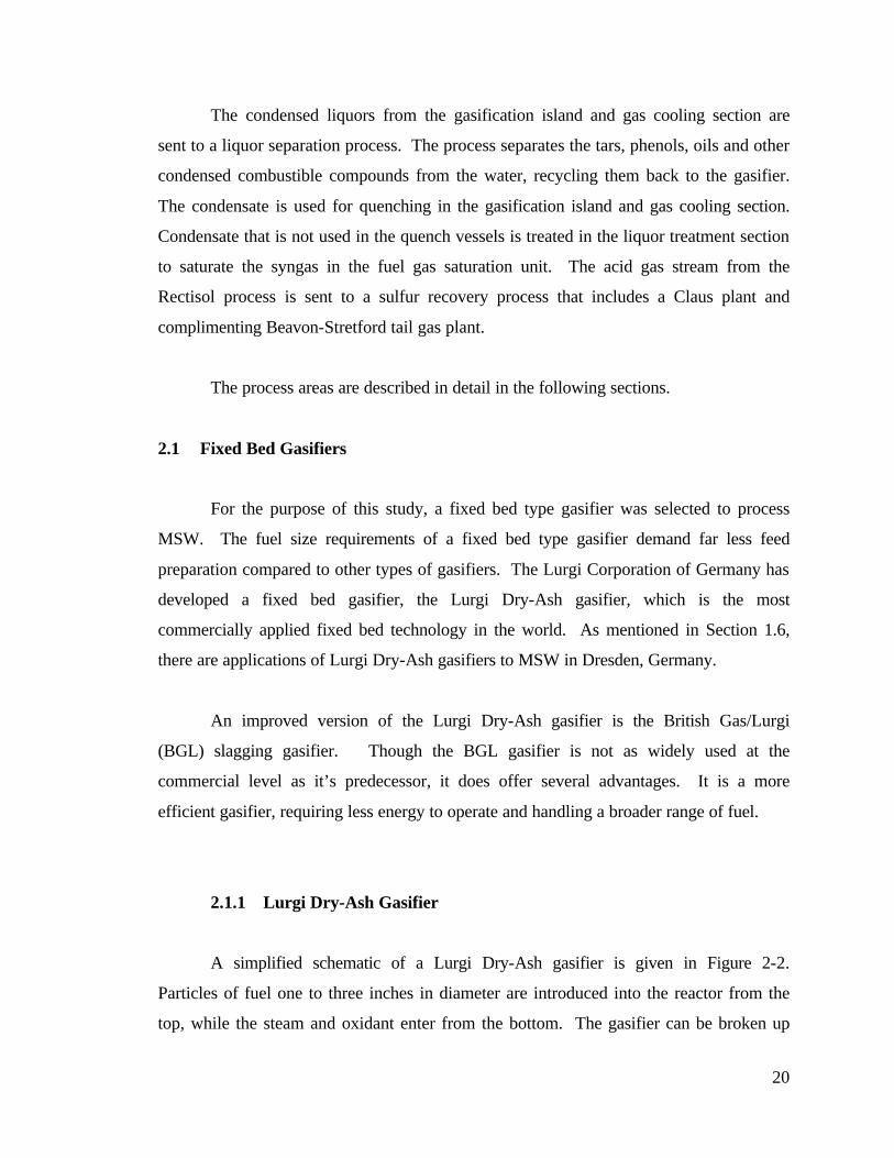
2.1.1 Lurgi Dry-Ash Gasifier

A simplified schematic of a Lurgi Dry-Ash gasifier is given in Figure 2-2.

Particles of fuel one to three inches in diameter are introduced into the reactor from the

top, while the steam and oxidant enter from the bottom. The gasifier can be broken up

21

into zones. In the first zone, drying, the coal is heated and dried while cooling the

product gas that is about to leave the reactor. This zone ranges from 575 - 1,100 °F. As

the coal descends into the hotter devolatilization zone, or carbonization zone, it is further

heated and devolatilized. In the gasification zone, the coal reacts with steam and carbon

dioxide (a product of the combustion zone) and the temperature is approximately 1,200 -

1,500 °F.

The combustion zone reaches the highest temperatures in the gasifier allowing the

oxygen to react with the char, providing the heat for the upper zones. In a dry-ash fixed

bed gasifier where the non-combustible material, the ash, is required to be solid, the

combustion zone temperature must be kept below the ash fusion temperature. In dry-ash

designs the temperature of the combustion zone is between 2,000 - 2,300 °F. At this

point, all that remains of the coal is the ash and char.

Product Gas

Drying and Devolitization Zone

Gasification Zone

Combustion Zone

Ash Zone

Fuel

Steam & Oxygen

Ash

Figure 2-2. Simple Schematic of a Fixed Bed Gasifier

22

The oxidant and steam are introduced into the gasifier through the bottom of the

vessel, also responsible for collecting ash. The oxidant and steam pass through the ash

where the reactants are heated. Simultaneously, the ash is cooled before being

discharged (Hebden and Stroud, 1981).

The lower temperatures in this type of gasifier, combined with methane

production in the devolatilization process, lead to a higher methane concentration in the

product gas. This relates to a higher heating value of the product. The oxidant, air or

oxygen, requirements are minimal in this method. The “cold gas efficiency” defined as

the ratio of sulfur-free gas Higher Heating Value (HHV) to the coal HHV is about 80

percent (Simbeck, 1983).

However, this process does produce hydrocarbon liquids, such as tars and oils,

limiting the ability to handle fines. In order to limit the amount of fines that are entrained

in the product gas, dusty tars, taken out in downstream separation processes, are recycled

back to the top of the gasifer. The dusty tars are believed to “stick” or conglomerate the

smaller fragments of the coal together, obtaining the necessary size requirements of the

gasifer. (Simbeck et al. 1983).

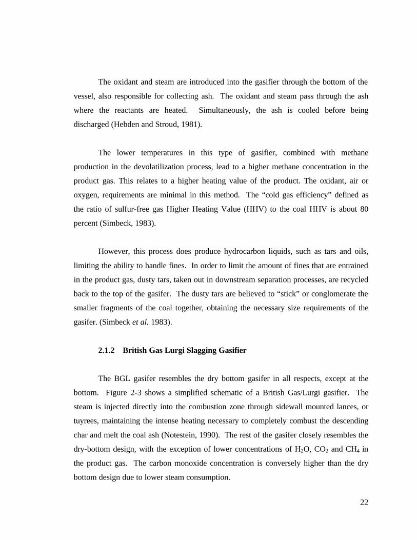
2.1.2 British Gas Lurgi Slagging Gasifier

The BGL gasifer resembles the dry bottom gasifer in all respects, except at the

bottom. Figure 2-3 shows a simplified schematic of a British Gas/Lurgi gasifier. The

steam is injected directly into the combustion zone through sidewall mounted lances, or

tuyrees, maintaining the intense heating necessary to completely combust the descending

char and melt the coal ash (Notestein, 1990). The rest of the gasifer closely resembles the

dry-bottom design, with the exception of lower concentrations of H2O, CO2 and CH4 in

the product gas. The carbon monoxide concentration is conversely higher than the dry

bottom design due to lower steam consumption.

23

Figure 2-3. Simplified Schematic of a BGL Slagging Gasifier

A key difference between the two gasifiers is that the BGL produces a liquid ash

(slag) while the dry ash produces a solid ash. In order for a dry-bottom gasifier to

operate, it must be kept below the ash melting point. Cooling is maintained with the

injection of excess steam. The large steam input lowers the thermal efficiency (Simbeck,

Devolatilizationand Drying100°F - 1300°F

Gasification1300°F- 2700°F

Combustion2700°F - 3600°F

Tuyeres

Quench

Quench Water In - 60°F

Quench Water Out - 140°F

Fuel

Dusty Tar Recycle

Syn-gas850°F

Quench Water

Slag Quench

Steam, Oxygen,Oils, Fines Recycle

Quench Syngas300°F

Wet Slag - 140°F

Slag

24

1983). With the BGL gasifer, the temperature must be above the ash melting point. The

temperature in the combustion zone is around 3,000 °F. This design uses about fifteen

percent of the steam that a dry-bottom gasifier consumes (Erdmann et al., 1999). The

higher temperatures of the BGL design result in higher conversion of the char in the

bottom of the gasifer. Therefore, the slag exiting the bottom of the gasifer is only 0.3-0.5

percent by weight carbon, while the ash exiting the dry-bottom design is 3-5 percent by

weight carbon (Vierrath, 1999)

Another key difference between the gasifiers is the ability to handle fines and

other components such as tars, oils, naphthas, phenols, etc., that may be entrained in the

product gas. The BGL gasifer can recycle tars, oils and fines through the tuyrees. Up to

30 percent of the coal feed has been in the form of fines through the tuyrees (Notestein,

1990). Tars, oils and fines are injected through the tuyrees, are introduced into the

gasifier at the hottest point. They are completely destroyed in the combustion zone,

having no chance of coming out entrained in the product gas. The cold gas efficiency of

the BGL gasifier is around 88 percent (Simbeck, 1983).

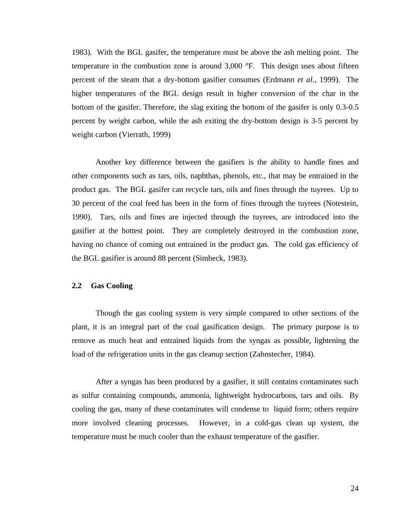
2.2 Gas Cooling

Though the gas cooling system is very simple compared to other sections of the

plant, it is an integral part of the coal gasification design. The primary purpose is to

remove as much heat and entrained liquids from the syngas as possible, lightening the

load of the refrigeration units in the gas cleanup section (Zahnstecher, 1984).

After a syngas has been produced by a gasifier, it still contains contaminates such

as sulfur containing compounds, ammonia, lightweight hydrocarbons, tars and oils. By

cooling the gas, many of these contaminates will condense to liquid form; others require

more involved cleaning processes. However, in a cold-gas clean up system, the

temperature must be much cooler than the exhaust temperature of the gasifier.

25

Though the Lurgi gasifier does not reach the temperatures that other gasification

systems reach, the temperature after the quench is still 300 °F. The required temperature

for the cold-gas clean up system is around 80 °F (Pechtl et al., 1992).

Figure 2-4 shows a simplified schematic of the gas cooling section. The sensible

heat of the crude syngas is removed by heating hot water for fuel gas saturation and

boiler feed water (BFW). The syngas is further cooled with quench water from the gas

liquor separation area. All liquors collected from the coolers are sent to the liquor

separation process.

Figure 2-4. Simplified Schematic of the Gas Cooling Process

2.3 Liquor Separation and Treatment

The liquor separation area receives the liquid streams from the gasifier and gas

cooling sections, separating and recycling combustible hydrocarbons that have condensed

out of the gasifier and gas cooling sections from the water. The liquid is utilized in the

quench systems of the gasification and gas cooling sections. Whatever liquid is not

needed for quenching, is treated in the liquid treatment facility and consumed in the fuel

gas saturation area.

IntermediateSyngas

HotSyngas

Condensed Liquors

Quench Water

CoolSyngas

SaturationWater

HotSaturation

Water

PreheatedBoiler Feed

Water

BoilerFeedWater

26

2.4 Gas Cleaning

Beside the typical contaminates common to all gasifiers (H2S, NH3, and COS),

the Lurgi gasifier produces large quantities of tar, oils, phenols and naphtha. Due to the

countercurrent flow of the Lurgi gasifier, the lowest temperatures in the gasifier are at the

top, where the syngas exits. Tars, phenols, oils, and naphtha are a result of the

devolatilization, or pyrolysis, zone in a gasifier. Since pyrolysis occurs at lower

temperatures than gasification, phenols, tars, naphtha and oils entrain in the gas before

reaching the gasification point in the gasifier, where they would be consumed.

Most of the oils, phenols, tars, NH3 and water condense out of the gas in the gas

cooling section. However, the gas cleaning section is required to remove naphtha, sulfur

containing compounds (H2S and COS) and trace phenols and oils.

In a BGL gasifier design, the phenols, naphtha and oils are recycled to the gasifier

through the tuyrees into the combustion zone for destruction. In both the BGL and Dry-

Ash designs, the tars are recycled back to the top of the gasifier to help conglomerate the

coal. In both cases it is important to recover these products out of the syngas.

In addition to sulfur compounds, CO2 also requires removal. Because of their

lower temperatures, Lurgi gasifiers typically produce more CO2 than other gasification

processes. Up to 30 mole percent of the crude syngas can consist of CO2 in a Lurgi

Gasifier. The liquid methanol process chosen for this project has had two design studies

varying the range of CO2 in the syngas feed from 2.5 mole percent (Air Products and

Chemicals, 1997) to 13 mole percent (Air Products and Chemicals, 1998). However, a

syngas with a CO2 range of 3-4 mole percent has provided the greatest conversion rates

of syngas to methanol (Air Products and Chemicals, 1998).

For this project, two processes of syngas cleanup were considered - the Rectisol®

process and Selexol® process. The three main differences between the two processes are

27

CO2 removal efficiency, solvent used and operating temperature. A third process, the

Purisol process, was not considered due to lack of design data availability.

2.4.1 Rectisol® Cleaning Method

The Rectisol® process is a Lurgi developed gas cleanup process, used in most

Lurgi gasification systems, including the waste facility in Germany. The process is also

used with a modified Texaco gasifier and the LPMEOHTM process in Kingsport,

Tennessee. The process uses methanol as it’s solvent to strip away sulfur containing

compounds and CO2 in a two-stage process. The first absorber strips away the sulfur

containing compounds; the second regenerates the methanol and absorbs the CO2. In the

report by Zahnstecher, the CO2 rich stream is sent to the CO2-rich gas incinerator.

Advantages of the Rectisol® process include:

• Pretreatment of solvent is not necessary because light hydrocarbons

can be separated easily from the methanol via azeotropic distillation.

• Since methanol is the solvent, it can be generated and re-cleaned in

house.

• Used in current Lurgi waste gasification facility.

• Used in the LPMEOHTM process at the Eastman Facility in Kingsport,

TN

The disadvantages are:

• Operates at a lower temperature, causing increase in energy costs.

• Not as widespread use as Selexol® and therefore extra risk and time

to develop model.

2.4.2 Selexol® Cleaning Method

The Selexol® gas purification process uses the solvent polyethylene glycol-

dimethylether. This solvent has a high molecular weight, high boiling point and can be

28

used at ambient temperatures. Lower temperatures increase the solubility of Selexol®

decreasing the circulation rate of the solvent, but drive up energy costs. The Selexol®

solvent requires pretreatment of gas to prevent solvent contamination by hydrocarbons

such as oil or naphtha.

The advantages for Selexol® are:

• Simple, proven process that has been modeled in ASPEN before.

• Operates at a higher temperature than the Rectisol® process, requiring

less energy.

The disadvantages are:

• Requires pretreatment of gas so that the solvent is not contaminated.

• Is not used in current Lurgi gasification systems

For this process, the Rectisol® cleanup system is used because according to

preliminary data from the Lurgi waste gasification plant, the CO2 levels coming out of

the gasifier are high. Preliminary data from the Berlin plant show an after gas cleanup

report with the CO2 composition around 8 percent (Vierrath, 1999). In a coal gasification

report by Zahnstecher utilizing the Lurgi process, the crude gas CO2 is 33 mole percent

while after the clean up CO2 is down to 1.5 mole percent. This shows the Rectisol®

process has a range of CO2 stripping ability.

The Selexol® process does remove some CO2 from the syngas, however it is

usually still present in the syngas at the upper limit of the methanol process, around 13

percent. The Selexol® process does use less energy than the Rectisol® process, but it

does not have the range of CO2 stripping ability of Rectisol®. Both processes do an

adequate job of sulfur removal. Lurgi reports that syngas from municipal waste

gasification has a high content of CO2. The methanol process has a range of CO2

concentration acceptability between 3-13 percent (Street, 1999). It is important that a gas

cleanup system has the ability to remove large amounts of CO2.

29

Additionally, Rectisol® is the only process that has “commercially demonstrated

the ability to remove sulfur to a level of 0.1 ppmv” (Biasca et al., 1987). Data is not

available as to which form the sulfur is in (e.g., H2S, COS, etc.) that the Rectisol®

process demonstrates this kind of removal efficiency, only that the process removes the

sulfur from the syngas.

2.5 Sulfur Recovery

A valuable byproduct of an IGCC system is sulfur. However, the emissions of

sulfur containing compounds into the atmosphere are strictly regulated due to

environmental hazards. As mentioned in Section 2.4, a gas cleaning process is an

integral section of an IGCC system not only for environmental regulations compliance

but also to recover combustible products and to avoid downstream equipment corrosion.

However, after the sulfur has been cleaned from the syngas, an acid gas remains,

containing sulfur compounds.

Recovery of elemental sulfur from the acid gas is done by a method called the

Claus process. The process produces a tail gas and elemental sulfur that is saleable,

recovering 90–95 percent of the sulfur. However, the Environmental Protection Agency

(EPA) requires that 99 percent of the sulfur in the raw gas is recovered. Thus, it is

necessary to employ a tail gas treatment system to recover additional sulfur. Further

treatment of the exhaust gas from the Claus process allows more sulfur is recovery in a

Beavon-Stretford tail gas treatment process.

2.5.1 Claus Process

The Claus process is a catalytic process that reacts H2S with SO2 to form

elemental sulfur, which can then be collected and sold. The tail gas from the Claus

process is further treated in the tail gas treatment plant described in Section 2.5.2. A

simplified schematic of the Claus process is illustrated in Figure 2-5.

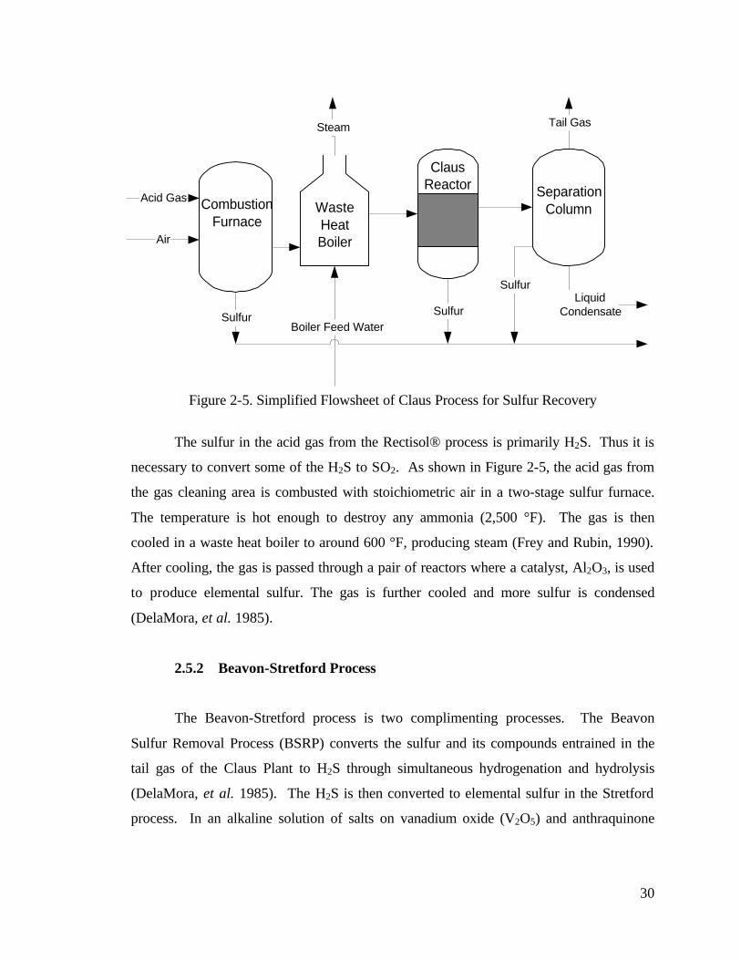
30

Figure 2-5. Simplified Flowsheet of Claus Process for Sulfur Recovery

The sulfur in the acid gas from the Rectisol® process is primarily H2S. Thus it is

necessary to convert some of the H2S to SO2. As shown in Figure 2-5, the acid gas from

the gas cleaning area is combusted with stoichiometric air in a two-stage sulfur furnace.

The temperature is hot enough to destroy any ammonia (2,500 °F). The gas is then

cooled in a waste heat boiler to around 600 °F, producing steam (Frey and Rubin, 1990).

After cooling, the gas is passed through a pair of reactors where a catalyst, Al2O3, is used

to produce elemental sulfur. The gas is further cooled and more sulfur is condensed

(DelaMora, et al. 1985).

2.5.2 Beavon-Stretford Process

The Beavon-Stretford process is two complimenting processes. The Beavon

Sulfur Removal Process (BSRP) converts the sulfur and its compounds entrained in the

tail gas of the Claus Plant to H2S through simultaneous hydrogenation and hydrolysis

(DelaMora, et al. 1985). The H2S is then converted to elemental sulfur in the Stretford

process. In an alkaline solution of salts on vanadium oxide (V2O5) and anthraquinone

Acid Gas

Air

Steam

Sulfur Sulfur

Sulfur

Tail Gas

LiquidCondensate

WasteHeatBoiler

CombustionFurnace

ClausReactor Separation

Column

Boiler Feed Water

31

disulfonate, the H2S is absorbed and oxidized to sulfur. The sulfur is then separated out,

washed and then melted to form a molten sulfur product.

2.6 Fuel Gas Saturation

In order to control NOx emissions from the gas turbine, the syngas is saturated

with water. Thermal NOx constitute a major fraction of the total NOx emissions from a

gas turbine. Since thermal NOx are extremely dependent on temperature, lowering the

peak flame temperature in the gas turbine controls their formation. By saturating the

syngas, the water vapor lowers the peak flame temperature.

Another advantage to saturating the syngas is that more power is produced from

the gas turbine. Saturating the syngas lowers its heating value. This results in an

increase of mass required to provide the gas turbine engine with the same amount of total

heating value. Because the mass flow of combustor gases is constrained by choked flow

at the turbine inlet nozzle, the compressor air has to be reduced to accommodate the

increase in syngas flow. This decreases the amount of work done by the compressors,

increasing the net output of power from the gas turbine.

The saturation vessel itself is a tray column, where the hot saturation water enters

from the top, while the syngas is introduced from the bottom. As the syngas rises

through the column, it absorbs water and is heated. Figure 2-6 shows a simplified

schematic of the fuel gas saturation process. The clean syngas from the gas cleaning area

enters the bottom of the column at about 80°F. After preheating with steam and BFW,

the saturation water is introduced at the top of the column. Steam is used to provide

additional heat to the saturator. Leaving the top of the saturator at about 350°F, the

syngas is then heated with hot BFW to 572°F before proceeding to the gas turbine. The

cooled water from the bottom of the tray column is collected and warmed in the gas

cooling section.

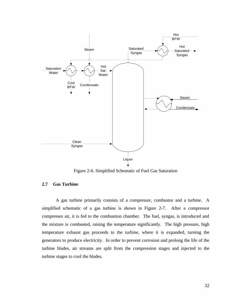
32

Figure 2-6. Simplified Schematic of Fuel Gas Saturation

2.7 Gas Turbine

A gas turbine primarily consists of a compressor, combustor and a turbine. A

simplified schematic of a gas turbine is shown in Figure 2-7. After a compressor

compresses air, it is fed to the combustion chamber. The fuel, syngas, is introduced and

the mixture is combusted, raising the temperature significantly. The high pressure, high

temperature exhaust gas proceeds to the turbine, where it is expanded, turning the

generators to produce electricity. In order to prevent corrosion and prolong the life of the

turbine blades, air streams are split from the compression stages and injected to the

turbine stages to cool the blades.

CleanSyngas

SaturatedSyngas

Liquor

HotSat.

Water

HotBFW

Steam

CoolBFW

Condensate

SaturationWater

Steam

Condensate

HotSaturatedSyngas

33

The gas turbine that is modeled in this study is a heavy duty “F” class unit, very

similar to a General Electric MS7001F. When firing syngas, the compressor ratio is

assumed to be 15.5, and a firing temperature in the combustion chamber of 2,350°F. The

turbine exhaust gas temperature is assumed to be around 1,100°F.

Figure 2-7. Simplified Schematic of a gas turbine

2.8 Steam Cycle

The steam cycle produces power for sale and steam for in-house use. It is

comprised of two sections, the HRSG and the steam turbine. The HRSG uses the

sensible heat of the gas turbine exhaust to provide energy, making steam. The steam is

used in a steam turbine to produce power as well as meet the steam demands of the rest of

the plant. A simplified schematic of the steam cycle is shown in Figure 2-8.

Generator

Air

Exhaust

CombustionChamber

Compressor Turbine

Cooling Stream

SHAFT

Fuel

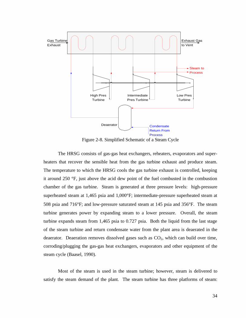
34

Figure 2-8. Simplified Schematic of a Steam Cycle

The HRSG consists of gas-gas heat exchangers, reheaters, evaporators and super-

heaters that recover the sensible heat from the gas turbine exhaust and produce steam.

The temperature to which the HRSG cools the gas turbine exhaust is controlled, keeping

it around 250 °F, just above the acid dew point of the fuel combusted in the combustion

chamber of the gas turbine. Steam is generated at three pressure levels: high-pressure

superheated steam at 1,465 psia and 1,000°F; intermediate-pressure superheated steam at

508 psia and 716°F; and low-pressure saturated steam at 145 psia and 356°F. The steam

turbine generates power by expanding steam to a lower pressure. Overall, the steam

turbine expands steam from 1,465 psia to 0.727 psia. Both the liquid from the last stage

of the steam turbine and return condensate water from the plant area is deaerated in the

deaerator. Deaeration removes dissolved gases such as CO2, which can build over time,

corroding/plugging the gas-gas heat exchangers, evaporators and other equipment of the

steam cycle (Baasel, 1990).

Most of the steam is used in the steam turbine; however, steam is delivered to

satisfy the steam demand of the plant. The steam turbine has three platforms of steam:

Steam toProcess

Gas TurbineExhaust

Exhaust Gasto Vent

CondensateReturn FromProcess

Deaerator

High PresTurbine

IntermediatePres Turbine

Low PresTurbine

35

(1) high; (2) intermediate; and (3) low pressure stages. The high-pressure steam is used

only in the first stage of the steam cycle. Both the second stage of the steam turbine and

the gasification island use the intermediate-pressure level steam. The low-pressure level

steam is utilized in the steam turbine and throughout the plant including: coal

preparation; gas liquor separation and treatment; gas cleaning; fuel gas saturation; and

sulfur recovery. In addition to satisfying the steam demand of the plant, the steam cycle

provides BFW for steam generation within other areas of the plant.

2.9 Liquid Phase Methanol Process

The production of methanol by a LPMEOHTM process involves three phases: (1)

the catalyst (solid phase); (2) inert hydrocarbon oil (liquid phase); and (3) the synthesis

gas (gas phase). The process is illustrated in Figure 2-9. The reaction takes place in a

fluidized bed reactor within the synthesis section of the methanol plant. The synthesis

gas, containing CO, H2, and CO2, is passed upward into the reactor concurrent with the

inert liquid hydrocarbon. At the top of the reactor, product gases separate leaving behind

the catalyst and liquid hydrocarbon. The heat generated in the reactor is used to make

high-pressure steam in the reactor’s internal heat exchanger. The effluent gases from the

reactor are then cooled and condensed. Unreacted gases are recycled after compression in

a recycle gas compressor. The methanol obtained can be purified by distillation to

produce chemical grade methanol.

The single pass conversion of syngas in LPMEOH™ reactor, though higher than

the conventional gas phase technology, is limited (Brown and Frenduto, 1992). For the

syngas richer in hydrogen, there is a lot of unconverted hydrogen after the methanol

reaction in LPMEOHTM reactor. Therefore, the unconverted syngas needs to be recycled

back to the reactor, to produce additional methanol. This scenario of methanol production

is known as LPMEOH™ process with recycle. There is also the once-through-methanol

(OTM) production. For this arrangement, the unreacted syngas (after a single pass

through LPMEOH™ reactor) is sent to a combustion facility for the generation of steam

(Street, 1999). In an IGCC system combined with LPMEOH™ process, the unconverted

36

syngas would be returned to the IGCC power plant gas turbines (Heydorn et al., 1998).

The reader is referred to Vaswani (1999) for detailed documentation of the plant

performance and emission model in ASPEN PLUS of the LPMEOHTM process area.

37

* Adapted from Vaswani, 2000

Figure 2-9. Simplified Schematic of the LPMEOH™ Process*

37

Purge gases

to boiler

Methanol

Mineral Oil

Catalyst

Guard Bed

LPMEOH Reactor

BFW

SteamSlurry Preparation Mixer

(Mineral oil and Catalyst mixing)

Recycle-gas compressor

Syngas

MethanolPurification

Recycle gas

Heat Exchanger

Economizer

Purge gases

to boiler

Methanol

Mineral Oil

Catalyst

Guard Bed

LPMEOH Reactor

BFW

SteamSlurry Preparation Mixer

(Mineral oil and Catalyst mixing)

Recycle-gas compressor

Syngas

MethanolPurification

Recycle gas

Heat Exchanger

Economizer

38

3.0 DOCUMENTATION OF THE PLANT PERFORMANCE AND EMISSION MODEL IN ASPEN PLUS OF THE BGL SLAGGING GASIFIER BASED IGCC SYSTEM

This chapter presents the performance model of the IGCC system featuring a

BGL slagging gasifier. The performance model, which calculates mass and energy

balances for the entire IGCC system, is implemented in ASPEN PLUS. The ASPEN

PLUS IGCC model consists of 153 unit operation blocks, 24 FORTRAN blocks and 32

design specifications. The ASPEN PLUS model unit operation blocks, FORTRAN

blocks and design specifications are described for each process area. The method for

calculating plant net thermal efficiency is described in detail. The sequencing of

calculations for each process area and for the entire model is explained in detail. Finally,

the methods used for modeling the air pollutant emissions from the system are discussed.

3.1 Overall Process Description

This performance model of the BGL Gasifier-based IGCC system is based

primarily on the findings of a study sponsored by the Electric Power Research Institute

(EPRI) (Pechtl et al., 1992). The EPRI sponsored study provides extensive information

regarding mass flows, temperatures, and pressures of streams as well as auxiliary power

requirements associated with each process area.

There are four major design differences between the ASPEN PLUS model and the

EPRI study. First, the gasifier is modified based on suggestions from Lurgi Umwelt

GmbH, FRG. The suggestions from Lurgi include less unreacted carbon in the slag and

the loss of sulfur through the slag. Second, the gas turbine has been tailored to reflect

current specifications. The model utilizes a heavy-duty General Electric MS7001F gas

turbine reflecting 1996 specifications while the EPRI study utilizes the same make and

model of gas turbine using 1992 specifications. While the EPRI study does not report the

firing temperature and pressure ratio of the gas turbine, the firing temperature for the

ASPEN PLUS model is 2,350 °F and the pressure ratio is 15.5, as described in Section

39

2.8. Third, the auxiliary loads for the Claus plant, Beavon-Stretford plant, air separation

plant and acid gas removal system are calculated independently of the EPRI study. The

Claus plant, Beavon-Stretford plant and air separation plant auxiliary loads are modeled

according to methods described by Frey and Rubin (1990) and the acid gas removal

system is modeled according to methods described by Eustis and Paffenbarger (1990).

The aforementioned alterations in auxiliary power load calculations more accurately

estimate the internal plant power consumption. The final design difference between the

model and EPRI study is the model uses the Rectisol® process to clean the syngas

instead of the Purisol process utilized in the EPRI study. Described in Section 2.4.1, the

Rectisol® process is advantageous over other gas cleaning processes because of its CO2

stripping ability.

Figure 3-1 illustrates how the sections of the plant are integrated to form the

complete IGCC system. The model consists of sections for gasification (Section 2.1), gas

cooling/acid gas removal (Sections 2.2 and 2.4, respectively), fuel gas saturation (Section

2.6), gas turbine (Section 2.7), HRSG and steam turbine (Section 2.8), liquor separation

(Section 2.3), methanol production (Section 2.9) and a Claus and Beavon-Stretford

treatment facility for sulfur recovery (Section 2.5). Also modeled are auxiliary power

requirements for each process area and for support facilities.

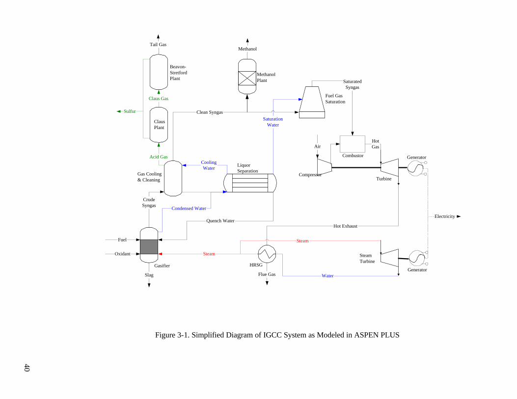
40

Figure 3-1. Simplified Diagram of IGCC System as Modeled in ASPEN PLUS

40

CrudeSyngas

Acid Gas

Slag

HotGasAir

Condensed Water

CoolingWater

Quench Water

SaturationWater

Clean Syngas

SaturatedSyngas

Hot Exhaust

Steam

WaterFlue Gas

Gas Cooling& Cleaning

Gasifier

LiquorSeparation

HRSG

CompressorTurbine

Combustor

MethanolPlant

SteamTurbine

Claus Gas

Tail Gas

Sulfur

Methanol

Fuel

Oxidant

ClausPlant

Beavon-StretfordPlant

Fuel GasSaturation

Electricity

Generator

Generator

Steam

41

3.2 Major Process Sections in the IGCC System

Each major process area of the IGCC plant is described in the following sections.

For each process area, an ASPEN PLUS flowsheet, a table describing the unit operations,

and a detailed description of the process area is provided. The user-specified inputs

indicated for each process area are specific to the EPRI base case described in Section

3.1. These values can be changed to represent alternate designs.

One of the general input requirements for the ASPEN PLUS performance model

is to choose a physical property data set. Within ASPEN PLUS there are several options

for such data sets. Each option uses either different data sources and/or different methods

for calculating thermodynamic properties. The property method used in the simulation is

the Peng-Robinson with Boston-Mathais alpha function option. This choice reflects the

recommendation of the ASPEN PLUS user manual for synthesis gas applications (Aspen

Tech®, 1993).

For each process area described in the following sections, a table is provided that

describes each unit operation block. The codes and terminology used in the tables are

explained in Appendix A.

3.2.1 Gasification Island

This section describes the gasification island, consisting of the BGL slagging

gasifier. The base case fuel is a typical Pittsburgh No. 8 coal as given in Table 3-1.

ASPEN PLUS has the capability to simulate solid materials as “non-

conventional” streams. Examples of non-conventional streams important to the IGCC

performance model are coal and MSW. In order to simulate non-conventional streams,

the user must enter an analysis of the stream composition such as an ultimate analysis, a

proximate analysis and a sulfur analysis (Rogers, 1994). The ultimate analysis

characterizes the material in terms of carbon, hydrogen, sulfur, oxygen, nitrogen and ash

42

Table 3-1. Proximate, Ultimate and Sulfur Analysis of Pittsburgh No. 8 Coal

Proximate Analysis, dry weight percent Moisture (actual weight percent) 6.00 Fixed Carbon 48.94 Volatile Matter 38.83 Ash 12.23 Ultimate Analysis, dry weight percent Carbon 73.12 Hydrogen 4.94 Nitrogen 1.38 Chlorine 0.09 Sulfur 3.30 Oxygen 4.85 Ash 12.23 Sulfur Analysis, weight percent Elemental 0.06 Pyritic 1.64 Organic 1.60 Higher Heating Value – Dry Basis (BTU/lb) 13,138

(Pechtl et al., 1992)

on a moisture-free weight percent basis. The proximate analysis includes the distribution

of a compound’s fixed carbon, volatile matter, ash and moisture on a weight percentage

basis. The sulfur analysis characterizes the distribution of total sulfur into inorganic,

pyritic and organic weight percentages (Thorsness, 1995).

ASPEN PLUS does not process non-conventional components (component is

used interchangeably with compound) in phase or chemical equilibrium calculations.

The program requires a chemical compound to be a “conventional” component, or a

component that is defined within ASPEN PLUS’s database, to use the compound in

phase or chemical equilibrium calculations. In order to handle solids, non-conventional

components and conventional components, ASPEN PLUS has several different stream

types. The stream type helps define the type of component. For solid components the

stream type is “CISOLID”, for a non-conventional component the stream type is “NC”

and for conventional components the stream type is “CONVENTIONAL”. ASPEN

PLUS allows one stream to have multiple types. For instance, the stream ELEMENTS in

the model has conventional, non-conventional and solid components in it, requiring

43

stream types “CONVENTIONAL”, “NC” and “CISOLID”. It is defined as stream type

“MIXCINC”.

Since the performance model simulates the gasification reactions with an

RGIBBS reactor, which is a chemical and phase equilibrium reactor, it is crucial that

ASPEN PLUS be able to process the fuel so that it can be properly characterized in the

RGIBBS reactor. To do this, the fuel must be broken down into its ultimate constituents

of elemental carbon, hydrogen, sulfur, oxygen, nitrogen, moisture and ash. This is

achieved using a FORTRAN block. Each of the elements are conventional constituents,

with the exception of ash, which is non-reactive, therefore ASPEN PLUS is able to

process the elements in the RGIBBS reactor. Using the input of the ultimate analysis and

proximate analysis, the FORTRAN block, MASSFLOW, determines the mass flow rates

of the elemental compounds. The fuel is now in a form that ASPEN PLUS can process

and use in phase and chemical equilibrium calculations.

After the completion of the FORTRAN block MASSFLOW, and the fuel has

been decomposed into its elements, ASPEN PLUS calculates the enthalpy of the stream

based on thermochemical data for carbon, hydrogen, sulfur, oxygen, nitrogen and water.

The enthalpy of the elemental coal stream is not the same as the enthalpy of the non-

conventional coal stream. Therefore, to maintain the energy balance, a FORTRAN

block, NRGFLOW, determines the difference in enthalpy of the two streams. This

difference is added back to the system at the GASIFXR block. A detailed description of

how ASPEN PLUS handles non-conventional component energy, along with a simple

case study illustrating the methodology, is provided in Appendix B.

Figure 3-2 illustrates unit operations and the mass flows in the gasification island

while Table 3-2 describes the unit operation blocks. The sequence of the gasification

island modeled in ASPEN PLUS begins with converting the fuel to “conventional”

compounds. In the ASPEN PLUS model, the fuel input is first converted into a form that

can be processed by downstream unit operations. Therefore, the inlet, non-conventional

44

Stream names are the same as those used in the ASPEN PLUS model. Unit Operation names are the same as block identification used in the ASPEN PLUS model.

Figure 3-2. ASPEN PLUS Flowsheet of the Gasification Island

ELEMENTS

VOLITLTODEVOL

INFINE

FEED GAS

SYNGAS

EXCARB

ASH

EXITGAS

LIQUOR

TAR

GAZ FINLGAS

COALFEED

BRKDWN

TOPGASIF

DEVOL

CSEP

ASHSEP

GASIFXRQHEAT

QCOMB

QGSLOSS

STEAM

OXIDANT

REHC

FLUX

BGLBFW

BGLBLDN

BGLSTM

QGSL

SLAG

SGAS

QNCHWTR

QUENCHDDBURN

STPGAS

O2

PRODGAS

DPROD

BOTTOM

GSCOOL

TARMIX

FLASH

JCKTSTMFrom

Oxygen PlantFrom

Steam Cycle

FromLiquor Separation

FromSteam Cycle

GSCOMB

QMIX

CLASS TARSEP

GSBURN

GSCOOL

DHEAT

QNCHHTLS

RETARFrom LiquorSeparation

To LiquorSeparation

ToDisposal

To GasCooling

ToSteam Cycle

ToSteam Cycle

44

45

Table 3-2. Gasification Section Unit Operation Block Description No BLOCK ID

(ASPEN BLOCK NAME)

BLOCK PARAMETERS

DESCRIPTION

1 BREAKDON (RYIELD)

Temperature = 77 °F Pressure = 400 psi

Yields of carbon, sulfur, hydrogen, nitrogen, oxygen, ash and water set by FORTRAN block MASSFLOW. Heat set by FORTRAN block NRGFLOW.

2

TOPGASIF (HEATX)

Hot Temp. = 850 °F

Simulates heat transfer between rising hot syngas and falling cold fuel.

3 DEVOL (RYIELD)

Pressure = 400 psi Duty = 0

The yield reactor simulates the formation of tar, phenol, oils and naphtha in the gasifier. The yields of tar, phenol, oils, naphtha, carbon, hydrogen and oxygen are set by the FORTRAN block PYROLIS.

4 CSEP (SEP2)

FRAC CISOLID INFINE SULFUR 0.97 EXCARB CARBON 0.004

Simulates the loss of carbon and sulfur due to unreacted char in gasifier.

5 COMB (RSTOIC)

Pressure = 400 psi Duty = 0

The stoichiometric reactor simulates the partial combustion of the carbon using all the oxygen in the feed. The steam, oxidant and recycle streams are added here.

6 GASIFXR (RGIBBS)

Temperature = 1300 °F Pressure = 400 psi

This reactor simulates the gasification zone through equilibrium calculations based on minimizing Gibbs free energy.

7 ASHSEP (SEP2)

FRAC NC ASH ASH 1.0 MIXED ASH CAO 1.0

This block separates the ash from the syngas

(Continued)

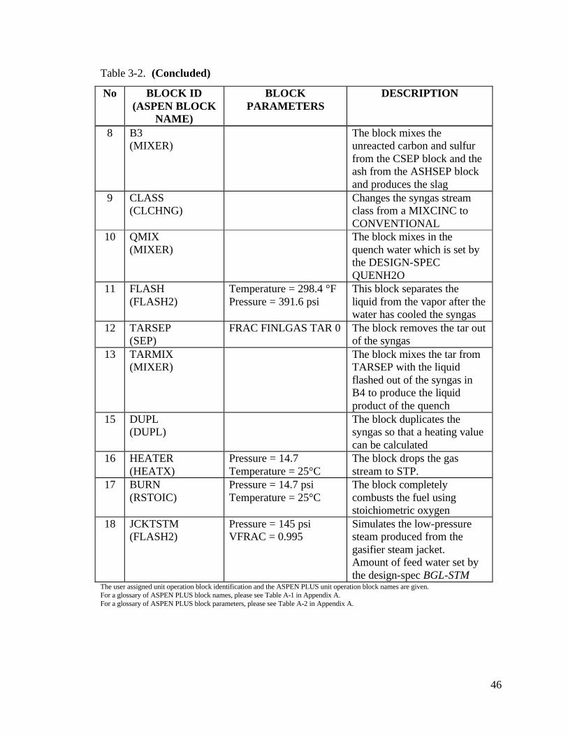
46

Table 3-2. (Concluded)

No BLOCK ID (ASPEN BLOCK

NAME)

BLOCK PARAMETERS

DESCRIPTION

8 B3 (MIXER)

The block mixes the unreacted carbon and sulfur from the CSEP block and the ash from the ASHSEP block and produces the slag

9 CLASS (CLCHNG)

Changes the syngas stream class from a MIXCINC to CONVENTIONAL

10 QMIX (MIXER)

The block mixes in the quench water which is set by the DESIGN-SPEC QUENH2O

11 FLASH (FLASH2)

Temperature = 298.4 °F Pressure = 391.6 psi

This block separates the liquid from the vapor after the water has cooled the syngas

12 TARSEP (SEP)

FRAC FINLGAS TAR 0 The block removes the tar out of the syngas

13 TARMIX (MIXER)

The block mixes the tar from TARSEP with the liquid flashed out of the syngas in B4 to produce the liquid product of the quench

15

DUPL (DUPL)

The block duplicates the syngas so that a heating value can be calculated

16 HEATER (HEATX)

Pressure = 14.7 Temperature = 25°C

The block drops the gas stream to STP.

17

BURN (RSTOIC)

Pressure = 14.7 psi Temperature = 25°C

The block completely combusts the fuel using stoichiometric oxygen

18 JCKTSTM (FLASH2)

Pressure = 145 psi VFRAC = 0.995

Simulates the low-pressure steam produced from the gasifier steam jacket. Amount of feed water set by the design-spec BGL-STM

The user assigned unit operation block identification and the ASPEN PLUS unit operation block names are given. For a glossary of ASPEN PLUS block names, please see Table A-1 in Appendix A. For a glossary of ASPEN PLUS block parameters, please see Table A-2 in Appendix A.

47

stream COALFEED is converted to a conventional stream, ELEMENTS, in the

FORTRAN block MASSFLOW. After the fuel has been broken down into its elements

by the FORTRAN block MASSFLOW, the RYIELD reactor BRKDWN computes the

yields of each of the elemental components. The FORTRAN block maintaining the

energy balance, NRGFLOW, is then executed.

Tars, oils and other high-weight hydrocarbons are entrained with the syngas in the

devolatilization zone of a fixed bed gasifier. The formation of the high-weight

hydrocarbons in the gasifier is modeled using a yield reactor, DEVOL, and FORTRAN

block PYROLIS. The model simulates the formation of the tars and oils that are

entrained in the syngas in the yield reactor DEVOL. The volatile matter is modeled in

ASPEN PLUS as TAR (C15H30-1, n-decyclopentane), PHENOL (C6H6O), OIL (C10H18

-1,

cis-decalin) and NAPHTHA (C11H10-1, 1-methylnaphthalene). The FORTRAN block

PYROLIS calculates the amount of high-weight hydrocarbons to create based on a user

specified mass fraction. The ASPEN PLUS user specifies a fraction of the mass flow rate

of the inlet fuel to the gasifier, COALFEED for each high-weight hydrocarbon as shown

in Equations (3-1) to (3-4):

YTAR = 0.04739 x mC,GI,I (3-1)

YPHENOL = 0.002463 x mC,GI,I (3-2)

YNAPHTHA = 0.007450 x mC,GI,I (3-3)

YOIL = 0.02031 x mC,GI,I (3-4)

where,

mC,GI,i = Mass flowrate of coal to gasifier, lb/hr

YTAR = Mass flowrate of tar in syngas, lb/hr

YPHENOL = Mass flowrate of phenol in syngas, lb/hr

YNAPHTHA = Mass flowrate of naphtha in syngas, lb/hr

YOIL = Mass flowrate of oil in syngas, lb/hr

The FORTRAN block PYROLIS then generates the hydrocarbons from the

carbon, hydrogen and oxygen in the stream ELEMENTS and sets the yield fractions in

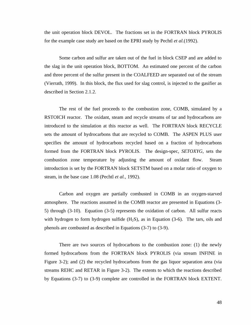
48

the unit operation block DEVOL. The fractions set in the FORTRAN block PYROLIS

for the example case study are based on the EPRI study by Pechtl et al.(1992).

Some carbon and sulfur are taken out of the fuel in block CSEP and are added to

the slag in the unit operation block, BOTTOM. An estimated one percent of the carbon

and three percent of the sulfur present in the COALFEED are separated out of the stream

(Vierrath, 1999). In this block, the flux used for slag control, is injected to the gasifier as

described in Section 2.1.2.

The rest of the fuel proceeds to the combustion zone, COMB, simulated by a

RSTOICH reactor. The oxidant, steam and recycle streams of tar and hydrocarbons are

introduced to the simulation at this reactor as well. The FORTRAN block RECYCLE

sets the amount of hydrocarbons that are recycled to COMB. The ASPEN PLUS user

specifies the amount of hydrocarbons recycled based on a fraction of hydrocarbons

formed from the FORTRAN block PYROLIS. The design-spec, SETOXYG, sets the

combustion zone temperature by adjusting the amount of oxidant flow. Steam

introduction is set by the FORTRAN block SETSTM based on a molar ratio of oxygen to

steam, in the base case 1.08 (Pechtl et al., 1992).

Carbon and oxygen are partially combusted in COMB in an oxygen-starved

atmosphere. The reactions assumed in the COMB reactor are presented in Equations (3-

5) through (3-10). Equation (3-5) represents the oxidation of carbon. All sulfur reacts

with hydrogen to form hydrogen sulfide (H2S), as in Equation (3-6). The tars, oils and

phenols are combusted as described in Equations (3-7) to (3-9).

There are two sources of hydrocarbons to the combustion zone: (1) the newly

formed hydrocarbons from the FORTRAN block PYROLIS (via stream INFINE in

Figure 3-2); and (2) the recycled hydrocarbons from the gas liquor separation area (via

streams REHC and RETAR in Figure 3-2). The extents to which the reactions described

by Equations (3-7) to (3-9) complete are controlled in the FORTRAN block EXTENT.

49

The extent that the reactions (3-7) to (3-9) are allowed to progress is limited to the

amount of the

1.013 C + O2 → 0.026 CO + .987 CO2 (3-5)

H2 + S → H2S (3-6)

C15H30 + 22.5 O2 → 15 CO2 + 15 H2O (3-7)

C10H18 + 14.5 O2 → 10 CO2 + 9 H2O (3-8)

C11H10 + 13.5 O2 → 11 CO2 + 5 H2O (3-9)

CaCO3 → CaO + CO2 (3-10)

recycled portion of the hydrocarbon. For example, if 10,000 lb/hr each of tars, naphtha

and oil are recycled to the combustion zone via streams REHC and RETAR, then the

reactions (3-7) to (3-9) would be limited to combusting only 10,000 lb/hr of each

compound in the streams REHC and RETAR (i.e. tar; oil; and naphtha). This way only

the recycled hydrocarbons are combusted leaving the newly formed tar, oil and naphtha

to proceed through the gasifier.

The calcium carbonate (CaCO3) is reduced in this reactor, as shown in Equation

(3-10). The heat from COMB is transferred to an RGIBBS reactor, used to simulate the

gasification zone of the gasifier.

The gasification zone, modeled in ASPEN PLUS with the unit operation block

GASIFXR, operates at a temperature of 1300 °F and a pressure of 400 psi (Vierrath,

1999). Equations (3-11) to (3-15) are specified to model the equilibrium of key

components such as CO, CO2, H2O, H2, NH3 and CH4. The following equilibrium

relations are assumed in the model:

C + H2O ↔ CO + H2 (3-11)

C + CO2 ↔ CO (3-12)

50

C + 2 H2 ↔ CH4 (3-13)

CO + H2O ↔ CO2 + H2 (3-14)

0.5 N2 + 1.5 H2 ↔ NH3 (3-15)

GASIFXR is an RGIBBS reactor. In an RGIBBS reactor, the temperatures of

specified reactions (e.g. Equations (3-11) to (3-15)) can be adjusted to calculate

equilibrium for each reaction at a specific temperature. Adjusting the approach

temperatures of the reactions represented by Equations (3-11) to (3-14), controls the

syngas composition. The FORTRAN block SETNH3 controls the extent of Equation (3-

15). The block provides a means for the to set the fuel nitrogen conversion to ammonia in

the gasifier.

The next unit operation block, ASHSEP, separates the ash and CaO from the

vapor. The resulting vapor is the crude syngas. The drying zone of the gasifier is

modeled with a heat exchanger block, TOPGASIF. The crude syngas from ASHSEP

exchanges heat with the incoming fuel to the gasifier in the unit operation block,

TOPGASIF. This heat exchanger block is specified so that the crude syngas outlet

temperature is 850 °F (Pechtl et al., 1992). Since all the “CISOLID” and “NC” stream

type components have been removed from the syngas, the unit operation block CLASS

changes the stream type from “MIXCINC” to “CONVENTIONAL”.

The syngas is then quenched to reduce the temperature before the Gas Cooling

area. To simulate the quenching of the syngas, the syngas is mixed with water from the

gas liquor separation section, as described in Section 3.2.2. The design-spec SETQUEN

controls the amount of quench water used based on the outlet temperature of the quench

vessel. The temperature of the gas is further dropped to 298.4 °F in a flash drum (Pechtl

et al., 1992). The flash drum, FLASH, separates the liquid from the vapor. After the

liquid water is flashed out, the tar in the syngas is separated in TARSEP. The liquid

stream and the tar stream are combined to simulate the dirty gas liquor that are processed

in the gas liquor separation area.

51

The crude syngas from TARSEP is duplicated in a DUPL block (a DUPL block

replicates a stream), allowing the calculation of the heating value of the syngas. For the

purpose of calculating the heating value, the syngas temperature is reduced to 25 °C and

the pressure is reduced to one atm. The syngas is then completely combusted with

oxygen at standard temperature and pressure (STP). The heater block, GSCOOL reduces

the syngas to STP; followed by the RSTOICH reactor, BURN. The unit operation block

BURN completely combusts the fuel at STP. The heating value of the raw syngas can be

calculated by dividing the heat produced from BURN by the volumetric flow rate of the

inlet fuel flow to BURN, stream STPGAS.

To simulate jacket cooling and simultaneous low-pressure steam production, the

heat produced in the block GASIFXR is transferred to a heater block, JCKTSTM.

JCKTSTM is specified to produce low-pressure saturated steam. In this case, the jacket

steam pressure is assumed to be 145 psia based on the low-pressure required by the steam

cycle, as described in Section 3.2.6. A design-spec, BGL-STM, sets the amount of jacket

steam produced. The user specifies the amount of heat lost by the gasifier in BGL-STM.

The amount of heat loss from the gasifier is calculated as a percentage of the product of

the coal mass flowrate and the dry coal’s higher heating value. Based on the user

percentage input, BGL-STM calculates the amount of steam generated by JCKTSTM. In

this study, the percentage was assumed to be 1.92 (Pechtl et al., 1992).

The solid non-combustible waste residue from the gasifier, the slag, is formed in

the model by combining the ash and CaO from the block ASHSEP, and the carbon and

sulfur from the block CSEP in the MIXER block BOTTOM.

3.2.2 Gas Cooling/Cleaning and Liquor Separation Area

This section describes the syngas cooling, cleaning and liquor separation section.

As described in Section 2.2, the Gas Cooling area cools the syngas to 90 °F for the gas

cleaning area. The Gas Cleaning section, described in Section 2.4, utilizes the Rectisol®

52

cleaning process to remove sulfur and other contaminates from the syngas. The liquor

separation area separates the combustible components that are dissolved in the liquor

from the gasification island. Figure 3-3 shows the ASPEN PLUS process flowsheet and

Table 3-3 describes the ASPEN PLUS unit operation blocks for the gas cooling/cleaning

and liquor separation area.

The syngas from the gasification island, stream HOTGAS, enters the gas cooling

section at 298.4 °F (Pechtl et al., 1992). The syngas is cooled by warming water from the

fuel gas saturation unit in the heat exchanger GCSATPRE. The design-spec,

GCSATH2O, adjusts the mass flowrate of the cooling water, FRSAT, to achieve a user

specified temperature of 204 °F for the syngas exiting GCSATPRE (Pechtl et al., 1992).

GCFLASH separates the condensed liquids from the syngas. The gas is further cooled

with condensate water from the steam cycle in the heat exchanger GCBFWPRE. Another

design-spec, CONDPRE, calculates the mass flowrate of FRCCYCLE necessary to cool

the syngas to 87.5 °F (Eustis and Paffenbarger, 1990). A quench stream, FGASLIQ,

further cools the syngas at the FLASH2 block GCFCOOL. A design-spec, GCQUENCH,

determines the amount of quench water necessary to cool the syngas to 86 °F. The block

GCFCOOL functions as a final cooling method particulate removal operation for the

syngas. The 87.5 °F corresponds to the exit temperature of the syngas from the heat

exchanger GCBFWPRE and the 86 °F corresponds to the exit temperature of the syngas

from the quench vessel GCFCOOL. Though only a temperature difference of 1.5 °F,

these two unit operations are modeled to accurately reflect the gas cooling section of the

design basis (Pechtl et al., 1992).

The Gas Cooling section is highly integrated with the rest of the IGCC system.

Water is used to cool the syngas from the fuel gas saturation area (GCSATPRE) and

steam cycle (GCBFWPRE). These heat exchangers not only function to cool the syngas,

but to heat the water for the respective process area.

All but one mass percent of the ammonia and all of the phenol are separated from

the syngas in the block, GCDIRTSEP. The condensate from the two coolers, GCFLASH

53

and GCFCOOL, and the ammonia/phenol mix from GCDIRTSEP are collected in a

collection drum simulated by GCLIQMX. The cooled syngas stream, COOLGAS, is

then sent to the Rectisol® acid gas cleanup unit.

54

Stream names are the same as those used in the ASPEN PLUS model. Unit Operation names are the same as block identification used in the ASPEN PLUS model.

Figure 3-3. ASPEN PLUS Flowsheet of the Gas Cooling/Cleaning and Liquor Separation Processes

GCFLASHGAS2

GAS3

GAS5

NH3PHEN

FRSAT

Hot Water

HOTGAS

WATER

From Fuel GasSaturation

To Fuel GasSaturation

COOLGAS

GCSTM

CLNGAS

CONDENS

SULFRCH

CO2RCH

NAPHRCH

To ClausPlant

To Vent

RECTISOL

FRCCYCLE

RETURN

From SteamCycle

GAS4

WATER2 To SteamCycle

GCLIQMX

GLSFEED

RETAR

EXPGAS

GASLIQ

TOGAS

TOCOOL

TOTREAT

To Power/ChemicalProduction

From SteamCycle

GCDRTSEP

To SteamCycle

To GasificationIsland

To GasCooling

To Treatment

GCFCOOL

GCBFWPRE

GASLIQ

GLSPLIT

GCSATPREFrom

GasificationIsland

To Beavon-Stretford Plant

54

55

Table 3-3. Gas Cooling and Cleaning Section Unit Operation Block Description No BLOCK ID

(ASPEN BLOCK NAME)

BLOCK PARAMETERS

DESCRIPTION

1 GCSATPRE (HEATX)

Cold Temp Out = 291.2 Heats the water used in the fuel gas saturation area.

2 GCFLASH (FLASH2)

Temperature = 200 °F Pressure Drop = -10 psia

Separates the liquids and vapors. The Transfer block GC-HEAT sets the temperature

3 GCBFWPRE (HEATX)

Cold Temp Out = 203 °F

Preheats the BFW condensate from the steam cycle.

4 GCFCOOL (FLASH2)

Temperature = 86 °F Pressure = 381.4 psia

Separates the liquids and vapors.

5 GCDIRTSEP (SEP)

FRAC of NH3 in COOLGAS set to 0.01 FRAC of PHEN in COOLGAS set to 0.00

Separates the phenol and ammonia from the syngas

6 GCLIQMIX (MIXER)

Combines all the liquid streams from the coolers for processing in gas liquor separation

7 RECTISOL (SEP)

CLNGAS T = 75 °F P = 400 psia FRAC H2S = .0001 CO2RCH T = 70 °F P= 16.0 psia SULFRCH T = 75 °F P = 25 psia FRAC CO2 = .015 CONDENS T = 140 °F P = 14.7 psia FRAC H2O = 1.0 NAPHRCH T = 75 °F P = 100 psia

This block separates the syngas into acid gas, naphtha gas, CO2 stream, condensate stream and clean gas.

8 GASLIQ (SEP)

RETAR FRAC TAR = 1.0 OIL=1.0 NAPH=1.0 PHEN=1.0 EXPGAS FRAC H2=1.0 CH4=1.0 H2O=3.714x10-5 H2S=0.3286 CO=0.3632 CO2=0.2321

Separates the non-combustible liquor and expansion gas from the hydrocarbons and tars that can be recycled to the gasifier.

(Continued)

56

Table 3-3. (Concluded)

No BLOCK ID (ASPEN BLOCK

NAME)

BLOCK PARAMETERS

DESCRIPTION

9 GLSPLIT (FSPLIT)

FRAC TOGAS = 0.8802 TOCOOL = 0.0388

Sets the amount of gas liquor required in the gas cooling and gasification island sections. The fraction is set in FORTRAN block DIRTYREC

The user assigned unit operation block identification and the ASPEN PLUS unit operation block names are given. For a glossary of ASPEN PLUS block names, please see Table A-1 in Appendix A. For a glossary of ASPEN PLUS block parameters, please see Table A-2 in Appendix A.

The Rectisol® cleaning unit separates the cooled syngas into a clean gas, an acid

gas, a naphtha rich gas, a condensate and a CO2 rich stream. Based on estimates from a

modeling study done at Stanford University, using the Rectisol® process in conjunction

with a Texaco type gasifier, steam and electric requirements were determined for the

process (Eustis and Paffenbarger, 1990). The specific utility consumption figures used

were:

Total Electric Use 0.267 kWh/lbmol syngas

Total Steam Use 1722 BTU/lbmol syngas

Minimum Steam Level saturated steam at 65 psia

The steam use is calculated based upon the required heat duty of the Rectisol®

process which is 1,722 BTU heat duty/ dry lbmol of syngas. The heat duty is met by

cooling saturated steam. The steam requirements are calculated by the FORTRAN block

RECTREQ. The enthalpy of saturated steam at 125 psia is 1194.9 BTU/lb (Felder,

1986). The steam requirement is calculated by Equation (3-16). The electricity demand

calculated is discussed in Section 3.3.4.

(3-16)

where,

iRDiRS Msyngasdrylbmol

lbSteamm ,,,, ..

441.1

=

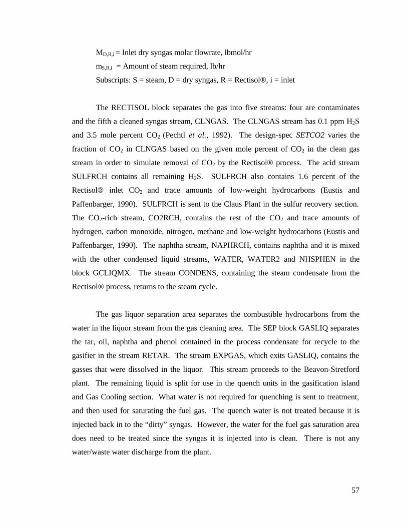
57

MD,R,i = Inlet dry syngas molar flowrate, lbmol/hr

mS,R,i = Amount of steam required, lb/hr

Subscripts: S = steam, D = dry syngas, R = Rectisol®, i = inlet

The RECTISOL block separates the gas into five streams: four are contaminates

and the fifth a cleaned syngas stream, CLNGAS. The CLNGAS stream has 0.1 ppm H2S

and 3.5 mole percent CO2 (Pechtl et al., 1992). The design-spec SETCO2 varies the

fraction of CO2 in CLNGAS based on the given mole percent of CO2 in the clean gas

stream in order to simulate removal of CO2 by the Rectisol® process. The acid stream

SULFRCH contains all remaining H2S. SULFRCH also contains 1.6 percent of the

Rectisol® inlet CO2 and trace amounts of low-weight hydrocarbons (Eustis and

Paffenbarger, 1990). SULFRCH is sent to the Claus Plant in the sulfur recovery section.

The CO2-rich stream, CO2RCH, contains the rest of the CO2 and trace amounts of

hydrogen, carbon monoxide, nitrogen, methane and low-weight hydrocarbons (Eustis and

Paffenbarger, 1990). The naphtha stream, NAPHRCH, contains naphtha and it is mixed

with the other condensed liquid streams, WATER, WATER2 and NHSPHEN in the

block GCLIQMX. The stream CONDENS, containing the steam condensate from the

Rectisol® process, returns to the steam cycle.

The gas liquor separation area separates the combustible hydrocarbons from the

water in the liquor stream from the gas cleaning area. The SEP block GASLIQ separates

the tar, oil, naphtha and phenol contained in the process condensate for recycle to the

gasifier in the stream RETAR. The stream EXPGAS, which exits GASLIQ, contains the

gasses that were dissolved in the liquor. This stream proceeds to the Beavon-Stretford

plant. The remaining liquid is split for use in the quench units in the gasification island

and Gas Cooling section. What water is not required for quenching is sent to treatment,

and then used for saturating the fuel gas. The quench water is not treated because it is

injected back in to the “dirty” syngas. However, the water for the fuel gas saturation area

does need to be treated since the syngas it is injected into is clean. There is not any

water/waste water discharge from the plant.

58

3.2.3 Sulfur Recovery

The sulfur recovery section consists of a Claus plant and a Beavon-Stretford tail

gas treatment plant. The model used for this area is based on a model developed by K. R.

Stone at Morgantown Energy Technology Center by the DOE (Stone, 1991). Figure 3-4

illustrates the sulfur recovery area and Table 3-4 describes the unit operation blocks used

in the model.

Air from the atmosphere is compressed in the COMP block, CAIRCOMP, to 23

psia (Stone, 1991). The amount of air supplied to the process is calculated by the design-

spec SETCLAIR by Equation (3-17).

MO2,C,i = 0.5 MH2S,C,i (3-17)

where,

MO2,C,i = Molar flow of oxygen in the inlet to CAIRCOMP, lbmol/hr

MH2S,C,i = Molar flow of H2S in stream from the Rectisol plant, lbmol/hr.

Subscript “C” indicates variable is from Claus Plant section

One-third of the H2S is then combusted in the RSTOIC reactor H2SCOMB1 as

shown in Equation (3-18). In the RSTOIC reactor H2SCOMB2, half of the SO2 is

converted to elemental sulfur as shown in Equation (3-19).

H2S + O2 → SO2 + H2O (3-18)

H2S + SO2 → H2O + S (3-19)

The stream is then cooled to 550°F by a HEATER block WHBOILER. Using the

heat produced, the FLASH2 block generates low-pressure steam. The design-spec

CLAUSTM varies the amount of steam produced to achieve zero heat loss from

CPSTEAM. Finally, the elemental product is separated from the tailgas by the SSPLIT

block CLAUSEP.

59

Stream names are the same as those used in the ASPEN PLUS model. Unit Operation names are the same as block identification used in the ASPEN PLUS model.

Figure 3-4. ASPEN PLUS Flowsheet of the Sulfur Recovery Process

CLAUSAIR

HPCAIR

TOCOMB2TOCOMB1 COMB2OUT

QWHBOIL

CLRXRIN

TAILGAS

CLXROUT

BSAIR

HPBSAIR HPTGAS

FLASHGAS

FUELGAS

BSCOMBIN HYDROIN TOSTRET STRETOUT

ACIDGAS

SULFRCH

CAIRCOMP

CLAUSMIX

SRCHG1

H2SCOMB1 H2SCOMB2

CLAUSRXR

CPSTM

WHBOILER

CLAUSEP

EXPGAS

TOB-S

SRCHG2

SRCHG3BSMIX

BSCOMPST HYDROXR STRETFRD

BSCOMP2

BSCOMP1

BSSEP

FromAtmosphere

FromAtmosphere

FromGas

Cleanup

FromLiquor

Separation

FromGas Cleanup

CPSTEAM

CPBLDN

CPBFW

CLAUSULF

BSSULF

OFFGAS

ToMarket

ToAtmosphere

ToSteam Cycle

59

60

Table 3-4. Sulfur Recovery Section Unit Operation Block Description No BLOCK ID

(ASPEN BLOCK NAME)

BLOCK PARAMETERS DESCRIPTION

1 CAIRCOMP (COMP)

TYPE = ISENTROPIC Pressure = 23 psia Isentropic Efficiency = 0.89

Compresses process air from the atmosphere to the required pressure

2 SRCHG1 (CLCHNG)

Block changes stream class from CONV to MIXCI

3 CLAUSMIX (MIXER)

Mixes process air with acid gas from Rectisol process

4 H2SCOMB1 (RSTOIC)

Temperature = 1722°F Pressure drop= 0 psia

Converts 1/3 of the H2S to SO2

5 H2SCOMB2 (RSTOIC)

Temperature = 1722 °F Pressure drop = 0 psia

Converts ½ of the SO2 to Sulfur

6 WHBOILER (HEATER)

Temperature = 550°F Pressure drop= 0

Cools the Claus gas and uses the heat to generate steam

7 CLAUSRXR (RSTOIC)

Temperature = 270 °F Pressure drop= 0 psia

Converts 94 percent of remaining H2S to Sulfur

8 CLAUSEP (SSPLIT)

TAILGAS FRAC MIXED = 1.0 CLAUSULF FRAC CISOLID = 1.0

Separates the solid sulfur product from the gaseous emissions of the Claus plant

9 CPSTM (FLASH2)

Pressure = 145 psia VFRAC = 0.995

Uses heat from WHBOILER to generate low pressure steam

10 BSCOMP1 (COMP)

TYPE = ISENTROPIC Pressure = 30 psia Isentropic Efficiency = 0.89

Compresses process air from the atmosphere to the required pressure

11 BSCOMP2 (COMP)

TYPE = ISENTROPIC Pressure = 30 psia Isentropic Efficiency = 0.89

Compresses the gaseous emissions from the Claus plant

12 SRCHG2 (CLCHNG)

Block changes stream class from CONV to MIXCI

13 SRCHG3 (CLCHNG)

Block changes stream class from CONV to MIXCI

14 BSMIX (MIXER)

Mixes process air, gaseous emissions from Claus plant, expansion gas from liquor separation and fuel gas

(Continued)

61

Table 3-4. (Concluded)

No BLOCK ID (ASPEN BLOCK

NAME)

BLOCK PARAMETERS DESCRIPTION

15 BSCOMPST (RSTOIC)

Temperature = 600 °F Pressure drop= 0 psia

Combusts the carbon compounds in the gas

16 HYDROXER (RSTOIC)

Temperature = 400 °F Pressure drop= 0 psia

Converts all the SO2 to H2S

17 STRETFRD (RSTOIC)

Temperature = 100 °F Pressure drop= 0 psia

Converts the H2S to solid Sulfur and water

18 BSSEP (SSPLIT)

OFFGAS FRAC MIXED = 1.0 BSSULF FRAC CISOLID = 1.0

Separates the solid sulfur product from the gaseous tail gas.

The user assigned unit operation block identification and the ASPEN PLUS unit operation block names are given. For a glossary of ASPEN PLUS block names, please see Table A-1 in Appendix A. For a glossary of ASPEN PLUS block parameters, please see Table A-2 in Appendix A.

For the Beavon-Stretford plant, the process air is compressed by BSCOMP1 to 30

psia (Stone, 1991). The amount of air required is determined by the design-spec

SETBSAIR from equation (3-20), for an explanation of coefficients, the reader is referred

to Stone, 1991.

MO2,BS,i = 1.01 (2 MCH4,BS,i + 0.5 MCO,BS,i + 0.5 MH2,BS,i + MSO2,BS,i) (3-20)

where,

MO2,BS,i = Molar flow rate of O2 at the inlet of BSCOMP1, lbmol/hr

MCH4,BS,i = Molar flow rate of CH4 in stream BSCOMBIN, lbmol/hr

MCO,BS,i = Molar flow rate of CO in stream BSCOMBIN, lbmol/hr

MH2,BS,i = Molar flow rate of H2 in stream BSCOMBIN, lbmol/hr

MSO2,BS,i = Molar flow rate of SO2 in stream BSCOMBIN, lbmol/hr

Subscript BS denotes Beavon-Stretford process area

The tail gas from the Claus plant is compressed to 30 psia by BSCOMP2 (Stone,

1991). The compressed air and Claus plant tail gas are mixed with clean syngas and the

expansion gases from the liquor separation area in the MIXER block BSMIX. The

combustible carbon compounds in the mixture BSCOMBIN are combusted in the

RSTOIC block BSCOMPST. All of the SO2 is then reduced to H2S in the block

HYRDOXR, according to Equation (3-21). The H2S and H2 are then converted to sulfur

62

and H2O, respectively, in the STRETFRD block according to Equations (3-22) and (3-

23), assuming 100 percent conversion (Stone, 1991).

SO2 + 3H2 → H2S + 2H2O (3-21)

H2S + ½O2 → H2O + S (3-22)

H2 + ½O2 → H2O (3-23)

The solid sulfur is separated from the gaseous emissions in the SSPLIT block

BSSEP. The combination of sulfur from the Claus plant and the Beavon-Stretford plant

can be sold as a product. The air emissions modeled from the sulfur recovery section are

CO2 and NH3 (Stone, 1991).

3.2.4 Fuel Gas Saturation

Saturating the fuel gas reduces the NOx emissions from the plant and increases the

power output from the gas turbine. The unit operation blocks are described in Table 3-5,

and the ASPEN PLUS flowsheet is illustrated in Figure 3-5.

After the removal of impurities and sulfur containing compounds, the syngas

enters the saturation area at 75°F and 400 psia. The syngas is duplicated in the DUPL

block CLNDUP. One stream determines the heating value of the clean syngas. For this

purpose syngas is cooled down to standard temperature and pressure (59°F and 14.7 psia)

in the HEATER block CLNHTR before combustion with stoichiometric oxygen in the

RSTOIC block CLNCOMB. The design-spec, CLNHV, determines the mass flow of the

stream CLNO2, the stoichiometric O2 stream.

63

Table 3-5. Fuel Gas Saturation Section Unit Operation Block Description No BLOCK ID

(ASPEN BLOCK NAME)

BLOCK PARAMETERS DESCRIPTION

1 CLNDUP (DUPL)

Duplicates the clean syngas stream to the saturation area

2 CLNHTR (HEATER)

Temperature = 59°F Pressure drop = 14.7 psia

Reduces the temperature and pressure to standard conditions

3 CLNCOMB (RSTOIC)

Temperature = 59°F Pressure drop = 14.7 psia

Combusts the clean syngas at STP to calculate the heating value

4 FGMIX (MIXER)

Mixes clean syngas with the purge gas from the LPMEOHTM process

5 FGBFWHT (HEATER)

Temperature = 350 °F Pressure drop = -20 psia

Cools BFW and captures the heat for use in saturation process

6 SIDEHEAT (HEATER)

Temperature = 355 °F VFRAC = 0.0

Condenses steam and captures heat for use in saturation process

7 FGPREHT (HEATER)

Temperature = 340 °F Pressure drop = -10 psia

Heats water from the gas cooling section with heat from steam

9 FGHEAT1 (HEATER)

Temperature = 340 °F Pressure drop = 0 psia

Supplies heat to warm the saturation water from cooling the water from the gas cooling section

10 FGHEAT2 (HEATER)

Temperature = 193.5°F Pressure drop = -5

Provides heat to saturation unit by cooling the water from the gas cooling section

11 FGPUMP (PUMP)

Pressure = 360 psia Pumps the saturation water to correct pressure

12 FGHEAT3 (HEATER)

Temperature = 193.5 °F Pressure drop = -5 psia

Heats the saturation water with heat from water from the gas cooling section

13 SIDEHT2 (HEATER)

Temperature = 222 °F Pressure drop = -5 psia

Heats the saturation water with heat from steam

14 FGBFWHT3 (HEATER)

Temperature = 420 °F Pressure drop = -5 psia

Heats the saturation water with heat from BFW

15 SATURTR (FLASH2)

Temperature = 369.2 °F Pressure drop = 350 psia

Simulates the saturation of the syngas

16 FGREHEAT (HEATER)

Temperature = 572.0 °F Pressure drop = -2 psia

Heats the saturated syngas with heat from BFW

(Continued)

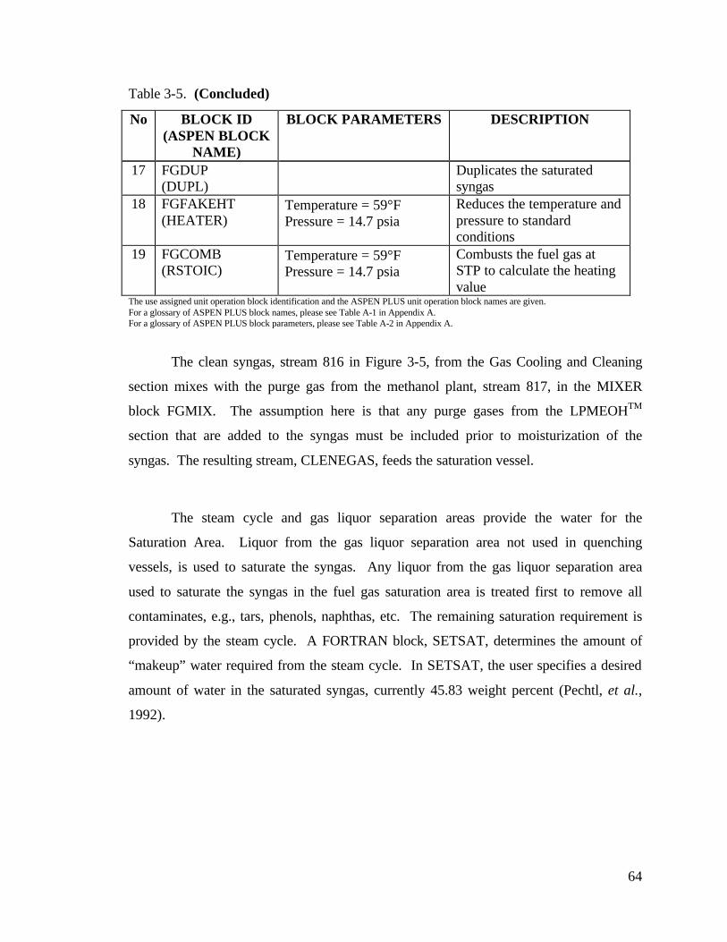
64

Table 3-5. (Concluded)

No BLOCK ID (ASPEN BLOCK

NAME)

BLOCK PARAMETERS DESCRIPTION

17 FGDUP (DUPL)

Duplicates the saturated syngas

18 FGFAKEHT (HEATER)

Temperature = 59°F Pressure = 14.7 psia

Reduces the temperature and pressure to standard conditions

19 FGCOMB (RSTOIC)

Temperature = 59°F Pressure = 14.7 psia

Combusts the fuel gas at STP to calculate the heating value

The use assigned unit operation block identification and the ASPEN PLUS unit operation block names are given. For a glossary of ASPEN PLUS block names, please see Table A-1 in Appendix A. For a glossary of ASPEN PLUS block parameters, please see Table A-2 in Appendix A.

The clean syngas, stream 816 in Figure 3-5, from the Gas Cooling and Cleaning

section mixes with the purge gas from the methanol plant, stream 817, in the MIXER

block FGMIX. The assumption here is that any purge gases from the LPMEOHTM

section that are added to the syngas must be included prior to moisturization of the

syngas. The resulting stream, CLENEGAS, feeds the saturation vessel.

The steam cycle and gas liquor separation areas provide the water for the

Saturation Area. Liquor from the gas liquor separation area not used in quenching

vessels, is used to saturate the syngas. Any liquor from the gas liquor separation area

used to saturate the syngas in the fuel gas saturation area is treated first to remove all

contaminates, e.g., tars, phenols, naphthas, etc. The remaining saturation requirement is

provided by the steam cycle. A FORTRAN block, SETSAT, determines the amount of

“makeup” water required from the steam cycle. In SETSAT, the user specifies a desired

amount of water in the saturated syngas, currently 45.83 weight percent (Pechtl, et al.,

1992).

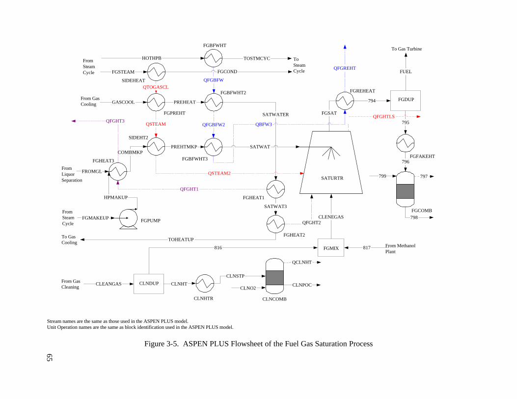
65

Stream names are the same as those used in the ASPEN PLUS model. Unit Operation names are the same as block identification used in the ASPEN PLUS model.

Figure 3-5. ASPEN PLUS Flowsheet of the Fuel Gas Saturation Process

FGSAT

794

FROMGL

PREHTMKP

TOHEATUP

GASCOOL

FGSTEAM

SATWATER

QFGHT2

HOTHPB TOSTMCYC

PREHEAT

SATWAT

QFGBFW2

QFGREHT

FromSteamCycle

ToSteamCycle

From GasCooling

To GasCooling

Saturator

CLEANGAS

QTOGASCL

QSTEAM

QSTEAM2

COMBMKP

QFGBFW

QBFW3

SATWAT3

QFGHT1

QFGHT3

HPMAKUP

FGMAKEUP

FromLiquorSeparation

CLNCOMB

816

From GasCleaning

CLENEGAS

817 From MethanolPlant

CLNDUP

CLNHTR

CLNHT

CLNSTP

CLNO2

FGDUP

FGFAKEHT

795

796

799

FUEL

CLNPOC

798

To Gas Turbine

QFGHTLS

FGCOND

FGCOMB

797

QCLNHT

FGMIX

FGPUMP

FGHEAT3

SIDEHT2

FGPREHT

SIDEHEAT

FGBFWHT

FGBFWHT2

FGHEAT1

FGHEAT2

FGBFWHT3

SATURTR

FGREHEAT

FromSteamCycle

65

66

The PUMP block FGPUMP raises the pressure of the makeup water from the

steam cycle, FGMAKEUP, to 360 psia. Both the water from the steam cycle,

HPMAKUP, and the treated liquor from the gas liquor separation Area, FROMGL, are

mixed together and heated in the HEATER block FGHEAT3. Further heating by

FGBFWHT3 raises the temperature to 420 °F before the saturation water enters the

saturation vessel, SATURTR.

Most of the unit operations utilized in this section are HEATER blocks used to

heat the syngas and saturation water. There are three main sources of heat: steam, high-

pressure BFW and water from the Gas Cooling Area. Shown by a red-dotted line in

Figure 3-5, steam provides heat to several HEATER blocks via heat streams:

QTOGASCL; QSTEAM; QSTEAM2; and QFGHTLS. Water from the Gas Cooling

Section and the saturation water are heated in the blocks FGPREHT and SIDEHT2,

respectively, with heat from steam. The saturation vessel also uses heat from steam from

the steam cycle. The design-spec, FGSTMREQ, determines the amount of steam

required, by setting the heat stream from the SATURTR, QFGHTLS to zero.

The amount of high-pressure BFW required by the saturation area is determined

in a similar fashion. The HEATER block, FGBFWHT, cools BFW from 597 °F to 350

°F, conveying energy to the process through the heat stream QFGBFW. From Figure 3-

5, the path the energy from cooling the high-pressure BFW is illustrated by the blue-

dotted heat streams: QFGBFW; QFGBFW2; QBFW3; and QFGREHT. The design-

spec, FGSTMREQ, determines the amount of high-pressure BFW by setting the heat

stream QFGREHT to zero.

After saturation in the FLASH2 block SATURTR, FGREHEAT heats the syngas

to 572 °F. To calculate the heating value of the saturated fuel, the DUPL block, FGDUP,

duplicates the saturated fuel stream for the blocks FGHAKEHT and FGCOMB. The

stream FUEL advances to the gas turbine.

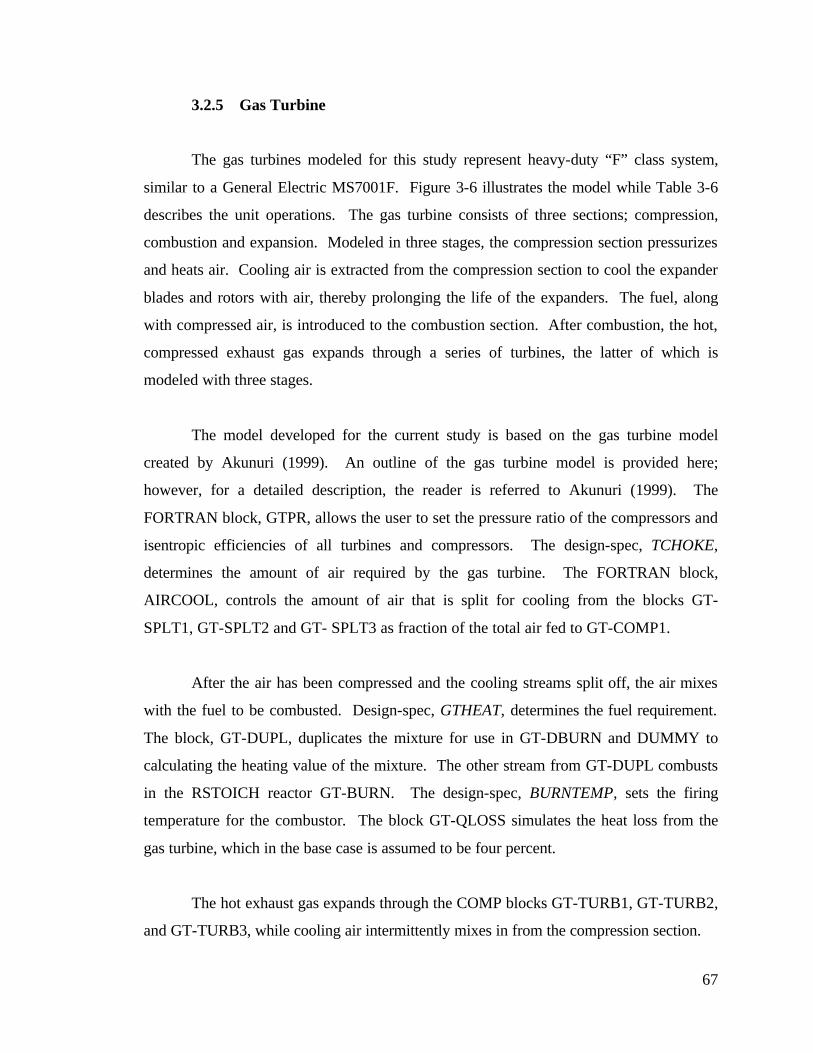
67

3.2.5 Gas Turbine

The gas turbines modeled for this study represent heavy-duty “F” class system,

similar to a General Electric MS7001F. Figure 3-6 illustrates the model while Table 3-6

describes the unit operations. The gas turbine consists of three sections; compression,

combustion and expansion. Modeled in three stages, the compression section pressurizes

and heats air. Cooling air is extracted from the compression section to cool the expander

blades and rotors with air, thereby prolonging the life of the expanders. The fuel, along

with compressed air, is introduced to the combustion section. After combustion, the hot,

compressed exhaust gas expands through a series of turbines, the latter of which is

modeled with three stages.

The model developed for the current study is based on the gas turbine model

created by Akunuri (1999). An outline of the gas turbine model is provided here;

however, for a detailed description, the reader is referred to Akunuri (1999). The

FORTRAN block, GTPR, allows the user to set the pressure ratio of the compressors and

isentropic efficiencies of all turbines and compressors. The design-spec, TCHOKE,

determines the amount of air required by the gas turbine. The FORTRAN block,

AIRCOOL, controls the amount of air that is split for cooling from the blocks GT-

SPLT1, GT-SPLT2 and GT- SPLT3 as fraction of the total air fed to GT-COMP1.

After the air has been compressed and the cooling streams split off, the air mixes

with the fuel to be combusted. Design-spec, GTHEAT, determines the fuel requirement.

The block, GT-DUPL, duplicates the mixture for use in GT-DBURN and DUMMY to

calculating the heating value of the mixture. The other stream from GT-DUPL combusts

in the RSTOICH reactor GT-BURN. The design-spec, BURNTEMP, sets the firing

temperature for the combustor. The block GT-QLOSS simulates the heat loss from the

gas turbine, which in the base case is assumed to be four percent.

The hot exhaust gas expands through the COMP blocks GT-TURB1, GT-TURB2,

and GT-TURB3, while cooling air intermittently mixes in from the compression section.

68

Stream names are the same as those used in the ASPEN PLUS model. Unit Operation names are the same as block identification used in the ASPEN PLUS model.

Figure 3-6. ASPEN PLUS Flowsheet of the Gas Turbine

GTAIR

AIR2GTCOOL1

AIR3

AIR4

GTCOOL2

AIR5

AIR6

AIR7

GTCOOL4

GTCOOL3

BURNFD BURN

DBURNPOC2

POC3

POC4

POC5

POC6

POC7

POC8

QBURN

QGTRECOV

QGTLOSS

WGT-C1

WGT-C2

WGT-T1

WGT-T2

WGT-C3

WGT-T3

WGASTRUB

FromSaturationArea FUEL

From Atmosphere

GT-COMP1 GT-COMP2 GT-COMP3

GT-SPLT1 GT-SPLT3GT-SPLT2

GT-MIXER

GT-MIX1

GT-MIX2 GT-MIX3

GT-MIX1

GT-TURB1GT-TURB2

GT-TURB3

GT-QLOSS

DUMMY

GT-DBURN

DBURN

QDBURN

DPOC2

LIQPOC3

WGTPOWER

GTPOC

To Steam Cycle

WGTLOSS

GT-WORK GT-POWER

QGTMIX1

GT-DUPL

GT-BURN

68

69

Table 3-6. Gas Turbine Section Unit Operation Block Description (Adapted from Akunuri, 2000)

No BLOCK ID (ASPEN BLOCK

NAME)

BLOCK PARAMETERS DESCRIPTION

1 GT-COMP1 (COMP)

TYPE = ISENTROPIC Pressure = 34.77 psia Isentropic Efficiency = 0.88

Compresses the air entering the gas turbine.

2

GT-SPLT1 (FSPLIT)

FRAC GTCOOL1 = 0.1

Block splits the compressed air coming out of the block GT-COMP1 and directs one stream to cool the products of combustion of the gas turbine.

3 GT-COMP2 (COMP)

TYPE = ISENTROPIC Pressure = 83.07 psia Isentropic Efficiency = 0.88

Similar to GT-COMP1.

4 GT-SPLT2 (FSPLIT)

FRAC GTCOOL2 = 0.1

Similar to GT-SPLT1. This corresponds to 1st stage rotor and 2nd stage vane cooling.

5 GT-COMP3 (COMP)

TYPE = ISENTROPIC Pressure = 227.85 psia Isentropic Efficiency = 0.88

Similar to GT-COMP1.

6 GT-SPLT3 (FSPLIT)

FRAC GTCOOL3 = 0.1 GTCOOL4 = 0.1

Similar to GT-SPLT1. This corresponds to 1st stage vane cooling.

7 GT-MIXER (MIXER)

The block mixes the compressed air and fuel gas.

8 GT-DUPL (DUPL)

Duplicates the mixed fuel and air stream for heating value calculation purposes.

9 GT-BURN (RSTOIC)

Temperature = 2,350 °F Pressure = 218.74 psia

Simulates the stoichiometric reactions that take place in the gas turbine combustor.

10 GT-DBURN (RSTOIC)

Temperature = 2,350 °F Pressure = 218.74 psia

Simulates the stoichiometric reactions that take place in a dummy gas turbine combustor.

11 GT-QLOSS (FSPLIT)

FRAC QGTLOSS = 0.5 FRAC QGTRECOV = 0.5

Simulates the loss of heat from the gas turbine combustor.

(Continued)

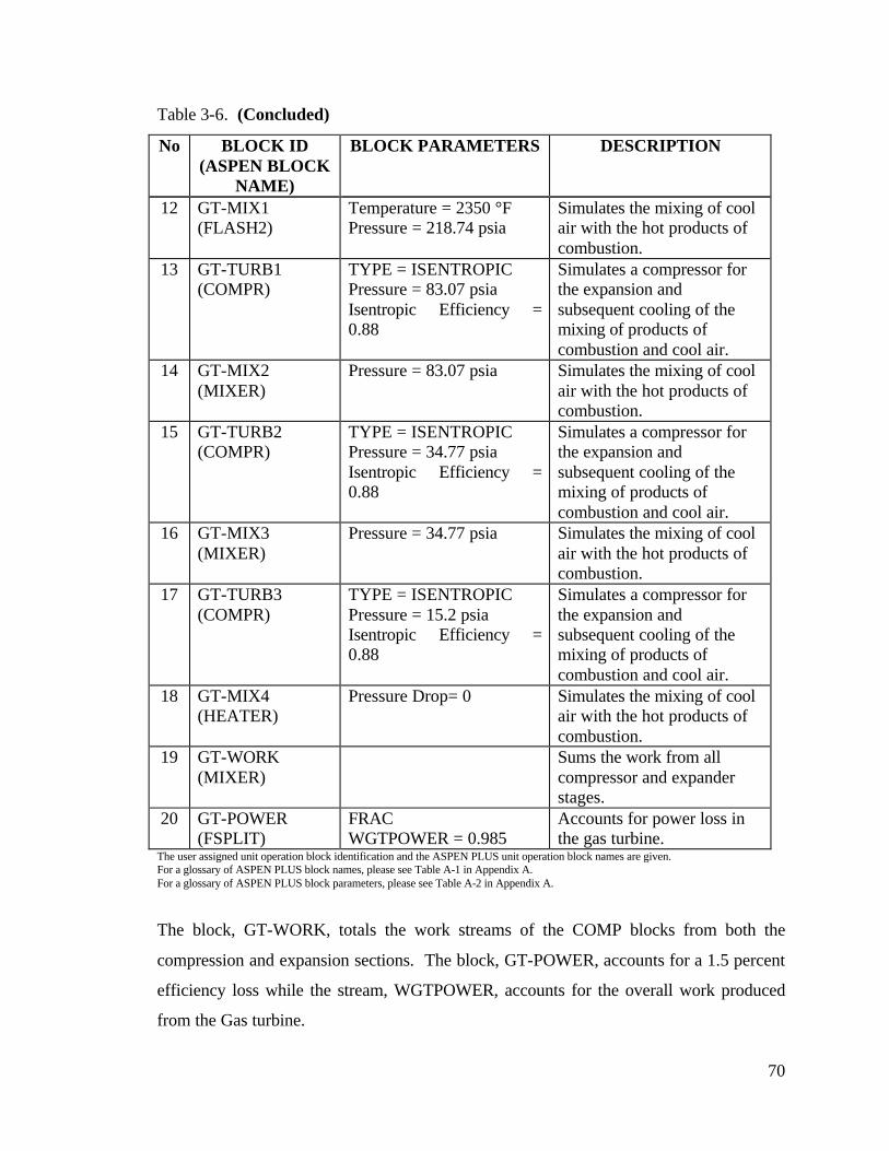
70

Table 3-6. (Concluded)

No BLOCK ID (ASPEN BLOCK

NAME)

BLOCK PARAMETERS DESCRIPTION

12 GT-MIX1 (FLASH2)

Temperature = 2350 °F Pressure = 218.74 psia

Simulates the mixing of cool air with the hot products of combustion.

13 GT-TURB1 (COMPR)

TYPE = ISENTROPIC Pressure = 83.07 psia Isentropic Efficiency = 0.88

Simulates a compressor for the expansion and subsequent cooling of the mixing of products of combustion and cool air.

14

GT-MIX2 (MIXER)

Pressure = 83.07 psia Simulates the mixing of cool air with the hot products of combustion.

15 GT-TURB2 (COMPR)

TYPE = ISENTROPIC Pressure = 34.77 psia Isentropic Efficiency = 0.88

Simulates a compressor for the expansion and subsequent cooling of the mixing of products of combustion and cool air.

16

GT-MIX3 (MIXER)

Pressure = 34.77 psia Simulates the mixing of cool air with the hot products of combustion.

17 GT-TURB3 (COMPR)

TYPE = ISENTROPIC Pressure = 15.2 psia Isentropic Efficiency = 0.88

Simulates a compressor for the expansion and subsequent cooling of the mixing of products of combustion and cool air.

18 GT-MIX4 (HEATER)

Pressure Drop= 0 Simulates the mixing of cool air with the hot products of combustion.

19 GT-WORK (MIXER)

Sums the work from all compressor and expander stages.

20 GT-POWER (FSPLIT)

FRAC WGTPOWER = 0.985

Accounts for power loss in the gas turbine.

The user assigned unit operation block identification and the ASPEN PLUS unit operation block names are given. For a glossary of ASPEN PLUS block names, please see Table A-1 in Appendix A. For a glossary of ASPEN PLUS block parameters, please see Table A-2 in Appendix A.

The block, GT-WORK, totals the work streams of the COMP blocks from both the

compression and expansion sections. The block, GT-POWER, accounts for a 1.5 percent

efficiency loss while the stream, WGTPOWER, accounts for the overall work produced

from the Gas turbine.

71

3.2.6 Steam Cycle

The steam cycle consists of two sections; the HRSG and the steam turbine. With

thirty-seven unit operation blocks, eight design-specifications, six FORTRAN blocks and

one transfer block, the steam cycle is the largest section of the model in ASPEN PLUS.

Table 3-7 describes the design-specifications while Table 3-8 specifies the unit operation

blocks. Because the steam cycle is so large, the ASPEN PLUS flow sheet is divided into

two parts. Figure 3-7 illustrates the HRSG section; Figure 3-8 shows the steam turbine

section.

Table 3-7. Steam Cycle Design-Specification Description Name Specification Variable Description

IPBFWPRO Massflow of stream IBFWPRO to IBREQ

Massflow of stream IPSPLIT in IPBFWSP

Determines the amount of intermediate-pressure BFW required by the process. IBREQ is the sum of the intermediate-press BFW plant requirements

IPCOOL Heat Stream QSTM116 to 0

Fraction of massflow to IPCOOL in IPBFWSP

Calculates the amount of BFW necessary to produce 145 psia steam for plant use.

LPROSTM Massflow of stream TORCTISL to REQS

Massflow of stream LPROSTM in SPLIT116

Calculates the amount of steam necessary to produce 145 psia steam for plant use. REQS is the sum of the 145 psia plant requirements.

SETBFW Heat Stream QXS to 0

Massflow of DEAERH2O

Calculates the amount of water in the steam cycle.

SETDSTM Heat Stream QDEAER to 0

Fraction of massflow to DEAERSTM in SPLIT29

Determines the amount of steam requried by DEAERATR block.

SETIPSTM Heat Stream QIPXS to 0

Fraction of massflow to IPBFW in BFWSPLIT

Determines the amount of water to the intermediate-pressure level.

SETLPSTM Heat Stream QLPXS to 0

Fraction of massflow to LPBFW in BFWSPLIT

Determines the amount of water to the low-pressure level.

STMQUAL Vapor Fraction of stream STEAM1 to 0.918

Isentropic Efficiency of HPTURB

Used to calibrate the amount of power generated by steam cycle.

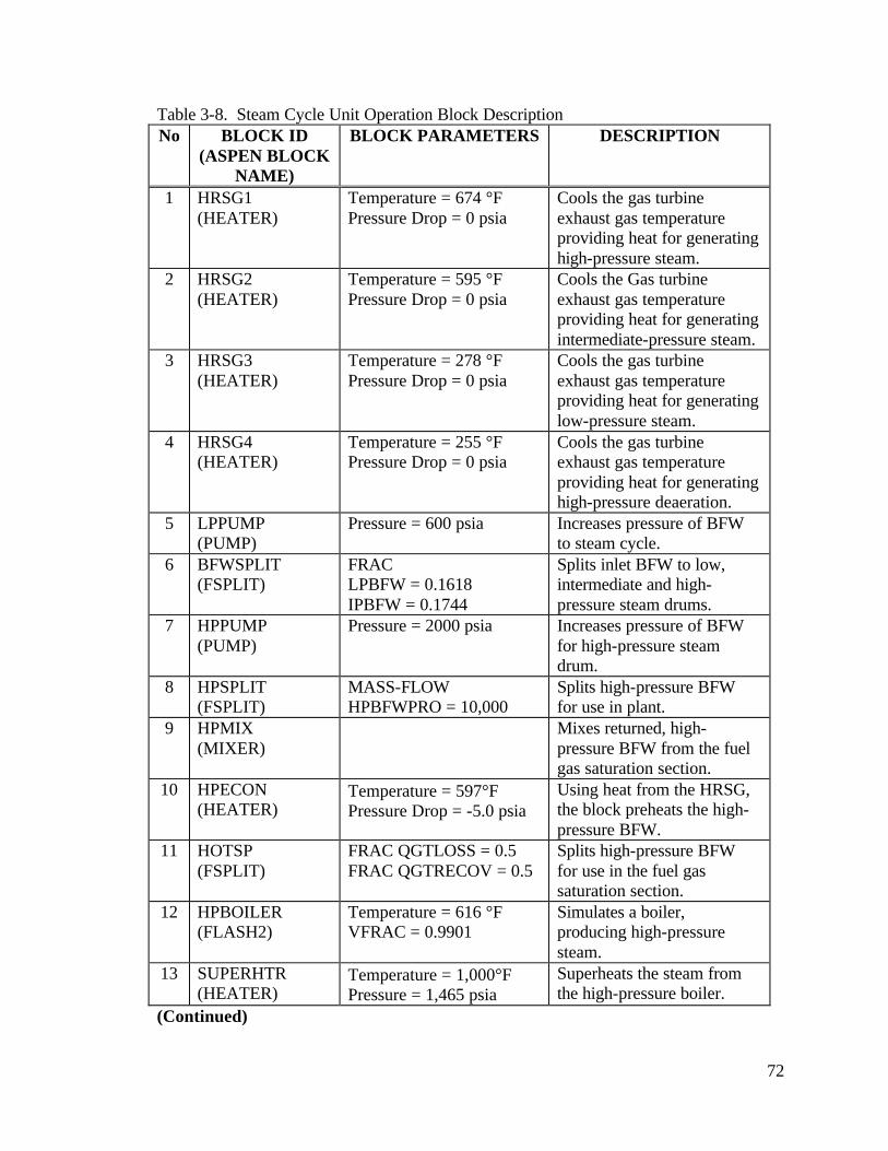
72

Table 3-8. Steam Cycle Unit Operation Block Description No BLOCK ID

(ASPEN BLOCK NAME)

BLOCK PARAMETERS DESCRIPTION

1 HRSG1 (HEATER)

Temperature = 674 °F Pressure Drop = 0 psia

Cools the gas turbine exhaust gas temperature providing heat for generating high-pressure steam.

2

HRSG2 (HEATER)

Temperature = 595 °F Pressure Drop = 0 psia

Cools the Gas turbine exhaust gas temperature providing heat for generating intermediate-pressure steam.

3 HRSG3 (HEATER)

Temperature = 278 °F Pressure Drop = 0 psia

Cools the gas turbine exhaust gas temperature providing heat for generating low-pressure steam.

4 HRSG4 (HEATER)

Temperature = 255 °F Pressure Drop = 0 psia

Cools the gas turbine exhaust gas temperature providing heat for generating high-pressure deaeration.

5 LPPUMP (PUMP)

Pressure = 600 psia Increases pressure of BFW to steam cycle.

6 BFWSPLIT (FSPLIT)

FRAC LPBFW = 0.1618 IPBFW = 0.1744

Splits inlet BFW to low, intermediate and high-pressure steam drums.

7 HPPUMP (PUMP)

Pressure = 2000 psia Increases pressure of BFW for high-pressure steam drum.

8 HPSPLIT (FSPLIT)

MASS-FLOW HPBFWPRO = 10,000

Splits high-pressure BFW for use in plant.

9 HPMIX (MIXER)

Mixes returned, high-pressure BFW from the fuel gas saturation section.

10 HPECON (HEATER)

Temperature = 597°F Pressure Drop = -5.0 psia

Using heat from the HRSG, the block preheats the high-pressure BFW.

11 HOTSP (FSPLIT)

FRAC QGTLOSS = 0.5 FRAC QGTRECOV = 0.5

Splits high-pressure BFW for use in the fuel gas saturation section.

12 HPBOILER (FLASH2)

Temperature = 616 °F VFRAC = 0.9901

Simulates a boiler, producing high-pressure steam.

13 SUPERHTR (HEATER)

Temperature = 1,000°F Pressure = 1,465 psia

Superheats the steam from the high-pressure boiler.

(Continued)

73

Table 3-8. (Continued)

No BLOCK ID (ASPEN BLOCK

NAME)

BLOCK PARAMETERS DESCRIPTION

14 HPTURB (COMPR)

TYPE = ISENTROPIC Pressure = 511 psia Isentropic Efficiency = 0.99

Simulates the high-pressure stage of the steam cycle turbine.

15 IPBFWSP (FSPLIT)

MASS-FLOW IPSPLIT = 10,000

Splits BFW water for use in plant, intermediate-pressure steam production and low-pressure process steam.

16 IPECON (HEATER)

Temperature = 461 °F VFRAC = 0

Using heat from the HRSG, the block preheats the BFW.

17 IPBOILER (FLASH2)

Temperature = 479 °F VFRAC = 0.9901

Simulates a boiler, producing intermediate-pressure steam.

18 IPSPRHTR (HEATER)

Temperature = 716 °F Pressure = 508 psia

Superheats the steam from the intermediate-pressure boiler.

19 STMMIX (MIXER)

Mixes the superheated intermediate-pressure steam with high-pressure steam.

20 SPLIT508 (FSPLIT)

MASS-FLOW TOGASIF = 12,000

Splits intermediate steam for use in gasification island.

21 REHEAT (FLASH2)

Temperature = 1,000 °F Pressure = 469 psia

Steam from the high-pressure turbine and intermediate-pressure boiler is superheated.

22 IPTURB (COMPR)

TYPE = ISENTROPIC Pressure = 116 psia Isentropic Efficiency = 0.90

Simulates the first-intermediate stage of the steam turbine.

23 SPLIT116 (FSPLIT)

MASS-FLOW LPROSTM = 10,000

Splits intermediate-pressure steam for use in plant.

24 116MIX (HEATER)

Temperature = 339 °F Pressure = 116 psia NPHASE = 1

Mixes steam intermediate-pressure steam with BFW to create steam for the plant.

25 LPTURB (COMPR)

TYPE = ISENTROPIC Pressure = 29 psia Isentropic Efficiency = 0.90

Simulates the second-intermediate stage of the steam turbine.

(Continued)

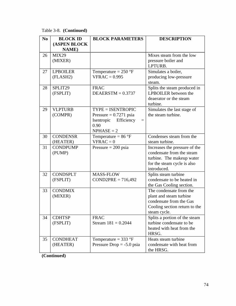
74

Table 3-8. (Continued)

No BLOCK ID (ASPEN BLOCK

NAME)

BLOCK PARAMETERS DESCRIPTION

26 MIX29 (MIXER)

Mixes steam from the low pressure boiler and LPTURB.

27 LPBOILER (FLASH2)

Temperature = 250 °F VFRAC = 0.995

Simulates a boiler, producing low-pressure steam.

28 SPLIT29 (FSPLIT)

FRAC DEAERSTM = 0.3737

Splits the steam produced in LPBOILER between the deaerator or the steam turbine.

29 VLPTURB (COMPR)

TYPE = ISENTROPIC Pressure = 0.7271 psia Isentropic Efficiency = 0.90 NPHASE = 2

Simulates the last stage of the steam turbine.

30 CONDENSR (HEATER)

Temperature = 86 °F VFRAC = 0

Condenses steam from the steam turbine.

31 CONDPUMP (PUMP)

Pressure = 200 psia Increases the pressure of the condensate from the steam turbine. The makeup water for the steam cycle is also introduced.

32 CONDSPLT (FSPLIT)

MASS-FLOW COND2PRE = 716,492

Splits steam turbine condensate to be heated in the Gas Cooling section.

33 CONDMIX (MIXER)

The condensate from the plant and steam turbine condensate from the Gas Cooling section return to the steam cycle.

34 CDHTSP (FSPLIT)

FRAC Stream 181 = 0.2044

Splits a portion of the steam turbine condensate to be heated with heat from the HRSG.

35 CONDHEAT (HEATER)

Temperature = 333 °F Pressure Drop = -5.0 psia

Heats steam turbine condensate with heat from the HRSG.

(Continued)

75

Table 3-8. (Concluded)

No BLOCK ID (ASPEN BLOCK

NAME)

BLOCK PARAMETERS DESCRIPTION

36 DEAERATR (FLASH2)

Pressure = 30 psia VFRAC = 0 NPHASE = 2

Simulates a dearation vessel that removes any entrained gases from the steam turbine condensate.

37 ST-MISC (MIXER)

Totals work done by pumps for calculating auxiliary power demands of the steam cycle.

38 ST-WORK (MIXER)

Totals work done produced by all stages of the steam turbine.

37 ST-POWER (MIXER)

Accounts for efficiencies in the gas turbine.

The user assigned unit operation block identification and the ASPEN PLUS unit operation block names are given. For a glossary of ASPEN PLUS block names, please see Table A-1 in Appendix A. For a glossary of ASPEN PLUS block parameters, please see Table A-2 in Appendix A.

3.2.6.1 Heat Recovery Steam Generator

The exhaust gas exits the gas turbine around 1,100 °F. The HRSG cools the gas

to approximately 250 °F, recovering the sensible heat in steam production. Four

HEATER blocks in ASPEN PLUS; HRSG1, HRSG2, HRSG3 and HRSG4 model the

HRSG. Each block cools the exhaust gas of the gas turbine, as described in Table 3-7.

The four HEATER blocks provide heat to four “trains” of heat requirements;

high-pressure steam generation, intermediate-pressure steam generation, low-pressure

steam generation and deaeration. HRSG1 provides heat to high-pressure steam

generation. HRSG1 provides heat to the blocks HPBOILER, SUPERHTR and REHEAT,

shown as red, dotted lines in Figure 3-7. HRSG2 provides heat for intermediate-pressure

level steam generation, which includes IPECON, IPBOILER and IPSPRHTR, shown in

Figure 3-7 as orange, dotted lines. The blue, dotted lines in Figure 3-7 illustrate the heat

HRSG3 provides for low-pressure steam generation, which includes the blocks HPECON

and LPBOILER. Finally, HRSG4 provides heat streams shown as green, dotted lines in

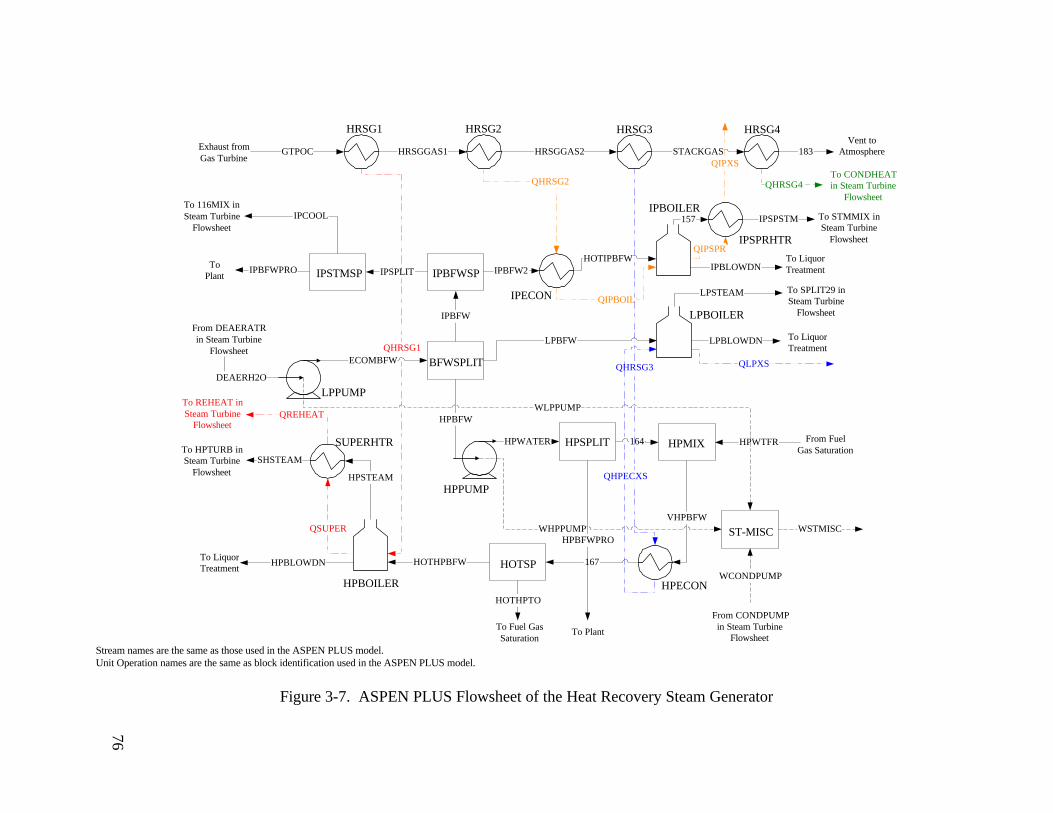
76

Stream names are the same as those used in the ASPEN PLUS model. Unit Operation names are the same as block identification used in the ASPEN PLUS model.

Figure 3-7. ASPEN PLUS Flowsheet of the Heat Recovery Steam Generator

HPECON

HRSGGAS1 HRSGGAS2 STACKGAS

ECOMBFW

IPBFW2HOTIPBFW

157

IPBFW

IPSPLIT

HPBFW

HPWATER 164

VHPBFW

167HOTHPBFW

HPSTEAM

QHRSG1

QSUPER

QHRSG2

QIPBOIL

QIPSPR

LPBFW

DEAERH2O

HPBLOWDN

SHSTEAM

QREHEAT

IPBFWPRO

HOTHPTO

IPSPSTM

QIPXS

IPCOOL

GTPOC

HPWTFR

LPSTEAM

LPBLOWDN

QHRSG3

QHPECXS

QLPXS

IPBLOWDN

183

To 116MIX inSteam Turbine

Flowsheet

ToPlant

From DEAERATRin Steam Turbine

Flowsheet

To REHEAT inSteam Turbine

Flowsheet

To HPTURB inSteam Turbine

Flowsheet

To Fuel GasSaturation

HPBFWPRO

To Plant

From FuelGas Saturation

To SPLIT29 inSteam Turbine

Flowsheet

To STMMIX inSteam Turbine

Flowsheet

Vent toAtmosphere

To LiquorTreatment

To LiquorTreatment

To LiquorTreatment

Exhaust fromGas Turbine

QHRSG4To CONDHEATin Steam Turbine

Flowsheet

HRSG1 HRSG2 HRSG3 HRSG4

LPPUMP

IPSTMSP IPBFWSP

BFWSPLIT

IPECON

IPBOILER

IPSPRHTR

LPBOILER

HPPUMP

HPSPLIT HPMIX

HOTSP

HPBOILER

SUPERHTR

WLPPUMP

WHPPUMP ST-MISC

WCONDPUMP

From CONDPUMPin Steam Turbine

Flowsheet

WSTMISC

76

77

Figure 3-7, for deaeration and condensate heating in the blocks DEAERATR and

CONDHEAT.

Liquid water, DEAERH2O, enters the steam cycle process area at 30 psia. The

design-spec, SETBFW, determines water requirements of the steam cycle. LPPUMP

pumps the water to 200 psia before splitting it to the three pressure levels by BFWSPLT.

The design-specs, SETLPSTM and SETIPSTM, determine the amount of water to the low-

and intermediate-pressure levels, respectively.

The low-pressure level consists of a boiler, LPBOILER, generating saturated

steam at 250 °F. The steam, used in the steam turbine, supplies heat to the deaerator.

To provide for the needs of the plant and to produce intermediate-pressure steam,

the intermediate-pressure level BFW splits in the block, IPBFWSP. IPBFWPRO

determines the plant’s water usage. The steam cycle needs intermediate-pressure BFW to

produce low-pressure steam; the amount is determined by the design-spec, IPCOOL. The

block, IPSTMSP, splits the water for use in the plant and steam cycle.

The water that proceeds from IPBFWSP to the steam cycle is heated to 461 °F in

IPECON, before being converted to 479 °F saturated steam in IPBOILER. IPSPRHTR

super-heats the steam to 716 °F and 508 psia before mixing with high-pressure steam in

STMMIX.

The block, HPPUMP, first pumps high-pressure BFW to 2,000 psia before the

block, HPSPLIT, splits it for use in the plant. The FORTRAN block, SETHPSTM,

calculates all high-pressure steam and BFW requirements. Although not used in this

design, the block, HPSPLIT, is used for integration with an air separation plant. High-

pressure BFW used for heating in the fuel gas saturation area, mixes with the high-

pressure BFW in HPMIX. The block, HPECON, heats the mixture to 597 °F. The

heating water, used in the fuel gas saturation area, splits out in block HOTSP.

HPBOILER creates 616 °F saturated steam, which is then super-heated by SUPERHTR

78

to 1,000 °F and 1,465 psia. This super-heated steam feeds the first stage of the steam

turbine, HPTURB.

3.2.6.2 Steam Turbine

From block SUPERHTR, the super-heated, high-pressure steam enters the first

stage of the steam turbine, HPTURB. The design-spec, STMQUAL, determines the

isentropic efficiency of HPTURB based on a specified outlet vapor fraction in the Steam

Turbine exhaust. This value is used to calibrate the Steam Turbine and is 0.918 in the

base case. The transfer block, SETSTEFF, sets the isentropic efficiencies of the

remaining turbine stages equal to HPTURB. The block, HPTURB, reduces the pressure

to 511 psia. The steam mixes with intermediate-pressure steam from IPSPRHTR in

STMMIX. The FORTRAN block, SETIPSTM, sets the amount of steam sent to the

gasification island by the block, SPLIT508. The amount of steam required of the

gasification island calculation is described in Section 3.2.1. After being reheated in the

block, REHEAT, to 1,000 °F, the steam proceeds to the second stage of the steam

turbine, IPTURB, expanding the steam to 116 psia. Calculated by the design-spec,

LPROSTM, the amount of steam required by the plant splits in the block, SPLIT116. The

block, 116MIX, cools the super-heated steam to 339 °F (saturated steam) with

intermediate-pressure level BFW. The design-spec, IPCOOL, calculates the amount of

intermediate-pressure BFW required to cool the steam. LPTURB further expands the

steam to 29 psia. After the steam from the low-pressure boiler splits to feed the

deaerator, the remaining steam mixes with the steam from LPTURB, in the block,

MIX29. The resulting mixture of MIX29 proceeds to the final stage of the steam turbine,

VLPTURB, where the pressure decreases to 0.7271 psia.

The block, CONDENSR, condenses the steam to 86 °F, while the block,

CONDPUMP, increases the pressure to 30 psia. Make-up water is also added at

CONDPUMP. The block, CONDSPLT, diverts a portion of the water for cooling water

in the Gas Cooling Section. The block, CONDMIX, combines plant condensate, and hot

water from the Gas Cooling Section, with the steam cycle water. The block, CDHTSP,

79

Stream names are the same as those used in the ASPEN PLUS model. Unit Operation names are the same as block identification used in the ASPEN PLUS model.

Figure 3-8. ASPEN PLUS Flowsheet of the Steam Turbine

STEAM511

STM511

REHTSTM

STEAM469

STEAM125STM2

LPROSTM

STEAM29

LPSTM

STEAM1

WATER1

WATER30

H2O30

178

181

182

179

QLPECXS

STM29

DEAERSTM

WVLPTURB

WLPTURB

WIPTURBWHPTURB

WSTMTURB

WSTPOWER

WSTLOST

SHSTEAM

IPSPSTM

TOGASIF

REHTLIQ

IPCOOL

QSTM116

SPLIT116

MIX29

SPLIT29

ST-WORK

ST-POWER

HPTURB

STMMIX

SPLIT508 REHEAT

IPTURB

116MIX

TORCTISL

LPTURB VLPTURB

CONDENSR

QCOND

MAKEUPCONDPUMP

CONDSPLT

COND2PRECONDMIXLPCNDPRO

HOTCOND

CDHTSP

QHRSG4

CONDHEAT

QDEAER

DEAERATR

DEAERVAP

DEAERLIQFrom

Process

ToProcess

From IPSPRHTRin HRSGFlowsheet

From SUPERHTRin HRSG Flowsheet

From IPSTMSPin HRSG Flowsheet

To LPPUMPin HRSGFlowsheet

From HRSG4in HRSGFlowsheet

To GasCooling

FromProcess

ToGasifier

LPSTEAMFrom LPBOILER

in HRSGFlowsheet

79

80

splits a portion of the condensate to be heated, in the block, CONDHEAT, before

entering the deaerator, modeled by the block DEAERTR. The deaerated water is then

sent back to LPPUMP.

3.2.7 Liquid Phase Methanol

Sudeep Vaswani developed the Liquid Phase Methanol Process model for

integration with the IGCC model. The combination of the IGCC model and the

LPMEOHTM model co-produces methanol and power. The LPMEOHTM model consists

of twenty-six unit operation blocks, four FORTRAN blocks and four design-specs. For a

detailed description of the LPMEOHTM model, the user is referred to Vaswani (2000).

3.3 Auxiliary Power Loads

Operations within the plant such as compressors, pumps and conveyor belts

consume significant amounts of electrical power, known as auxiliary power loads.

Because these operations employ power otherwise sent to the power grid for sale, the

auxiliary loads greatly affect the overall plant efficiency. Auxiliary power loads are

functions of process variables through the system. Select pumps and compressors are the

only auxiliary power loads modeled In ASPEN PLUS. The FORTRAN block,

AUXILARY, models all other auxiliary loads separately, which are described by plant

area in this section.

3.3.1 Coal Preparation

Using a study by Pechtl et al. (1992), an auxiliary power consumption model was

developed for coal preparation. Coal preparation is divided into two parts: coal receiving

and storage; and coal preparation and briquetting. Coal receiving and storage includes

coal unloading, conveying and stacking equipment. Coal preparation and briquetting

includes fuel screening, drying, conveying and pressurization equipment associated with

81

briquetting the coal. The coal feed rate chosen is the independent variable for

development of the auxiliary power model. Figures 3-9 and 3-10 graphically model the

data points for the coal receiving and storage and coal preparation and briquetting,

respectively. In kW, Equation (3-24) and (3-25) respectively show models for coal

receiving and storage (WRS) and coal preparation and briquetting (WPB).

WRS = 0.00312 mC,GI,i (3-24)

WPB = 0.002635 mC,GI,i (3-25)

where,

281,000 < MCOAL < 311,000 lb/hr as received coal

Equation (3-24) has an R2 = 1.00 and a standard error of the estimate is 1.81 kW,

and Equation (3-25) has an R2 = 0.991 and a standard error of the estimate is 1.10 kW.

However, the R2 is not surprising since only three data points were used to obtain the

equation. Two of these data points are so close to each other relative to the third that they

act like one data point. The total power required for the Coal Preparation Area is the sum

of Equations (3-24) and (3-25).

Figure 3-9. Power Requirement for Coal Receiving and Storage

Coal Receiving and Storage

860

880

900

920

940

960

980

275 280 285 290 295 300 305 310 315

As-Received Coal (1,000 lb/hr)

Po

wer

Co

nsu

mp

tio

n (

kW)

EPRI TR-100376

Linear (EPRI TR-100376)Model

82

Figure 3-10. Power Requirement for Coal Preparation and Briquetting

3.3.2 Gasification Island

The auxiliary power requirement for the gasification island includes pumps and

compressors for the feed and equipment for slag handling. According to a study by

Pechtl et al. (1992), a single point is available regarding the auxiliary power consumption

for the gasification island. The coal feed rate to the gasifier is taken to be the

independent variable. Equation (3-26) shows the auxiliary power model, in kW, for the

gasification island (WGI).

WGI = 0.00324 mC,GI,i (3-26)

3.3.3 Gas Liquor Separation and Treatment

For the gas liquor separation model, the auxiliary power model was developed

with 4 data points from a study by Pechtl et al. (1992). In the gas liquor separation

section the mass flowrate was used as the independent variable. Equation (3-27) shows

Coal Preparation and Briquetting

730740750760770780790800810820830

275 280 285 290 295 300 305 310 315

As-Received Coal (1,000 lb/hr)

Po

wer

Co

nsu

mp

tio

n (

kW)

EPRI TR-100376

Linear (EPRI TR-100376)Model

83

the auxiliary power model, in kW, for the gas liquor separation Area (WGS). Figure 3-11

is a graphical representation of the regression model.

WGS = 0.00111 mGS,GC,I (3-27)

where,

mGS,GC,i = Mass flowrate of gas liquor to gas liquor area, lb/hr

538,000 < mGS,GC,< 595,000 lb/hr gas liquor

Equation (3-27) has an R2 = 0.912 and the standard error of the estimate is 65.6 kW.

Figure 3-11. Power Requirement for the Gas Liquor Separation Area

The auxiliary power for the Gas Liquor Treatment area was developed using a

single data point from a study by Pechtl et al. (1992). Equation (3-28) shows the

auxiliary power model, in kW, for the Gas Liquor and Treatment area (WGT).

WGT = 0.00429 mT,GC,I (3-28)

where,

mT,GC,i = Mass flowrate of gas liquor for treatment, lb/hr

Gas Liquor Separation

575

600

625

650

675

530 540 550 560 570 580 590 600

Liquor Processed (1,000 lb/hr)

Po

wer

Co

nsu

mp

tio

n

(kW

)

EPRI TR-100376

Linear (EPRI TR-100376)Model

84

3.3.4 Rectisol®

The electrical requirements for the Rectisol® gas cleaning process was adapted

from Eustis and Paffenbarger (1990), as discussed in Section 3.2.2. Equation (3-29)

shows the electricity required, in kW, for the Rectisol® gas cleaning process (WRECT).

WRECT = 0.267 MR,GC,o (3-29)

where,

MR,GC,o = Molar flowrate of dry, clean syngas, lbmole/hr

3.3.5 Fuel Gas Saturation

In the fuel gas saturation section of the ASPEN PLUS model, the unit operation

block FGPUMP calculates the amount of work necessary to pump saturation water. The

auxiliary load for the fuel gas saturation area (WFGS) is calculated by multiplying the

work done by FGPUMP by a factor of 1.5, as in Equation (3-30). The factor of 1.5

calibrates the auxiliary power load to the design-basis and accounts for other operations

that may be used in the fuel gas saturation area that are not modeled in ASPEN PLUS.

WFGS = 1.5 WFGPUMP (3-30)

where,

WFGPUMP = Work done by FGPUMP, kW

3.3.6 Boiler Feed Water Treatment

A single data point from a study by Pechtl et al. (1992) is used to estimate the

auxiliary power consumption for the treatment of BFW. The make up water to the steam

cycle is the independent variable. Equation (3-31) shows the auxiliary power model, in

kW, for the BFW treatment (WBFWT).

85

WBFWT = 0.00119 mMU,SC,I (3-31)

where,

mMU,SC,i = Mass flowrate of makeup BFW to steam cycle, lb/hr

3.3.7 Power Island

The pumps modeled in ASPEN PLUS primarily account for auxiliary power loads

for the power island (WPI), including the gas turbine and steam cycle. Equation (3-32)

shows the calibration with the design basis, by the modification of the sum of the work

done by the pumps, with a factor of 1.2. As in Section 3.3.5, the factor of 1.2 in Equation

(3-32) accounts for the auxiliary loads not accounted for by the pumps in the ASPEN

PLUS model. The 0.7457 in Equation (3-32) is a conversion factor for horsepower to

kW.

WPI = 1.2 (WCOND + WLPUMP + WHPUMP) 0.7457 (3-32)

where,

WCOND = Work done on the pump which delivers condensate at 30 psia in HP

WLPUMP = Work done on the pump which delivers BFW at 200 psia in HP

WHPUMP = Work done on the pump which delivers BFW at 2,000 psia in HP

3.3.8 Liquid Phase Methanol Plant

The power consumption of the recycle, purge and feed compressors, given by

Equation (3-33), accounts for the auxiliary power loads for the LPMEOHTM plant (WME)

in kW.

WME = WFEED + WRECY + WPURG (3-33)

where,

WFEED = Work done on the compressor for the feed to the LPMEOHTM Plant, kW

WRECY = Work done on the compressor for the recycle stream in the LPMEOHTM

plant, kW

86

WPURG = Work done on the compressor for the purge gas from the LPMEOHTM

plant, kW

The amount of power required by these compressors is simulated in the ASPEN

PLUS model of the LPMEOHTM process.

3.3.9 Other Process Areas

For other areas of the plant such as oxidant feed, Claus and Beavon-Stretford

plants and general facilities, the auxiliary power loads are calculated based on regression

models developed by Frey and Rubin (1990). For the convenience of the reader the

models are briefly described. Further details can be found in Frey and Rubin (1990).

3.3.9.1 Oxidant Feed

The power required to separate oxygen from air, for the gasifier, is the largest

auxiliary power load in the IGCC system. The auxiliary power consumption model for

the oxidant feed was originally developed by Frey and Rubin (1990) and was modified by

Akunuri (1999) to reflect the latest published data. The auxiliary power model for the

oxidant feed (WOX) is given, in kW, in Equation (3-34).

WOX = (0.9466 + 3.73 x 10-4 TA + 9.019 x 10-6 TA2) *

(0.00526 MOX,GI,i)(1000)

(3-34)

where,

MOX,GI,i = Oxygen molar flowrate to the gasifier, lbmol/hr

TA = Ambient Temperature = 59 °F

3.3.9.2 Claus Plant

Equation (3-35) gives the auxiliary power load of the Claus Plant (WCP) in kW,

using 20 data points with R2 = 0.870.

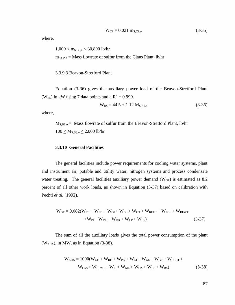
87

WCP = 0.021 mS,CP,o (3-35)

where,

1,000 < mS,CP,o < 30,800 lb/hr

mS,CP,o = Mass flowrate of sulfur from the Claus Plant, lb/hr

3.3.9.3 Beavon-Stretford Plant

Equation (3-36) gives the auxiliary power load of the Beavon-Stretford Plant

(WBS) in kW using 7 data points and a R2 = 0.990.

WBS = 44.5 + 1.12 MS,BS,o (3-36)

where,

MS,BS,o = Mass flowrate of sulfur from the Beavon-Stretford Plant, lb/hr

100 < MS,BS,o < 2,000 lb/hr

3.3.10 General Facilities

The general facilities include power requirements for cooling water systems, plant

and instrument air, potable and utility water, nitrogen systems and process condensate

water treating. The general facilities auxiliary power demand (WGF) is estimated as 8.2

percent of all other work loads, as shown in Equation (3-37) based on calibration with

Pechtl et al. (1992).

WGF = 0.082(WRS + WPB + WGI + WGS + WGT + WRECT + WFGS + WBFWT

+WPI + WME + WOX + WCP + WBS)

(3-37)

The sum of all the auxiliary loads gives the total power consumption of the plant

(WAUX), in MW, as in Equation (3-38).

WAUX = 1000(WGF + WRF + WPB + WGI + WGL + WGT + WRECT +

WFGS + WBFWT + WPI + WME + WOX + WCP + WBS)

(3-38)

88

3.3.11 Net Power Output and Plant Efficiency

The net power output of the plant is calculated by subtracting the auxiliary power

consumption of the plant from the gross power output. Since the IGCC system modeled

here produces two different products, electricity and methanol, the power output and

plant efficiency are can be calculated several different ways, such as:

• no credit for methanol production, considering only electricity as the

product

• full credit for methanol production, assuming 100 percent of the heating

value of methanol is recovered

• assume that the methanol is used to generate electricity and about � of the

energy is recovered

• assume that methanol is used as a fuel for automobiles and about ¼ of the

energy is recovered

• calculate the approximated IGCC electrical equivalent, about 42 percent,

of the heating value is recovered

For this study, the power output and plant efficiency are calculated two ways. One

method is to assume that electricity is the sole product of the plant and take no credit for

methanol production as in Equation (3-39). This method represents the lowest possible

efficiency because the plant receives no credit for the syngas that was consumed by the

methanol plant to make methanol:

MWnet = MWGT + MWST - WAUX (3-39)

where,

MWnet = Plant power to grid, MW

MWGT = Power generated by the gas turbine, MW

MWST = Power generated by the steam turbine, MW

The other method used to determine the power output is to take full credit (100

percent recovery) for the energy contained in the methanol as well as the net electrical

89

power production, as shown in Equation (3-40). The heating value, calculated in the

ASPEN PLUS model by completely combusting the methanol, is multiplied by the

amount of methanol produced to obtain the energy methanol contains. This method

overestimates the power production because it is not possible to recover 100 percent of

the energy from the methanol:

MWnet = MWGT + MWST + MWME - WAUX (3-40)

where,

MWME = Energy value of methanol, MW

For either case, Equation (3-41) gives the net plant efficiency on a higher heating

value basis.

HHV

MWnet

××=

iGI,C,

6

m10414.3η

(3-41)

where,

HHV = Higher Heating Value of fuel, BTU/lb

η = Net plant efficiency

The plant efficiency and power output are reported these two ways to give the full

range of possible efficiencies and outputs. The actual efficiency/output of the plant lies

somewhere between the values reported in this thesis, based on what the methanol is used

for.

3.4 Convergence Sequence

Each process area description in Section 3.2 includes the process area’s

convergence sequence. This section describes how all of the individual process areas are

sequenced to form the complete IGCC plant. There are three design-specs and one

FORTRAN block on which the convergence sequence for the entire IGCC system is

based. The amount of fuel required for the system, and the subsequent size of the IGCC

plant, is based on the amount of methanol produced and the size of the gas turbine. The

90

default assumed plant size includes two gas turbines in parallel and production of 10,000

lb/hr of methanol. Each gas turbine produces approximately 190 MW. Figure 3-12

illustrates the convergence sequence for the IGCC system.

The FORTRAN block GTPR sets the input assumptions for the gas turbine and is

the first block called in the overall convergence sequence. The design-spec TCHOKE is

then initialized to set the amount of air required by the gas turbine. After the compressor

section of the gas turbine is sequenced, the design-spec, GTHEAT, is initialized. As

mentioned in Section 3.2.5, the design-specs, GTHEAT and TCHOKE, determine the

amount of fuel and air required by the gas turbine, respectively.

After the convergence of the gasification island, the gas cooling/cleaning section

and the liquor separation area, a design-spec, LP-PROD, is initialized to set the amount

of methanol produced. The design-spec, LP-PROD, varies the fraction of clean syngas,

split in the FSPLIT block GC-SPLIT to the methanol plant based on a required

production rate for methanol. The LPMEOHTM and fuel gas saturation areas are called

before the remaining section of the gas turbine is simulated. After the sulfur recovery

and steam cycle sections are converged, the FORTRAN block AUXILARY calculates the

power consumption of each process area.

The model is sequenced in the previously described manner so that the user can

determine the overall size of the plant by specifying the amount of power and/or

methanol produced. To alter the power output of the IGCC plant, the user can either

adjust the size of the gas turbine or simulate multiple gas turbines in the design-spec

GTHEAT. The user determines the amount of methanol produced in the design-spec LP-

PROD. The model calculates all other feed and output streams including the amount of

fuel fed to the gasifier and the air requirement of the gas turbine(s).

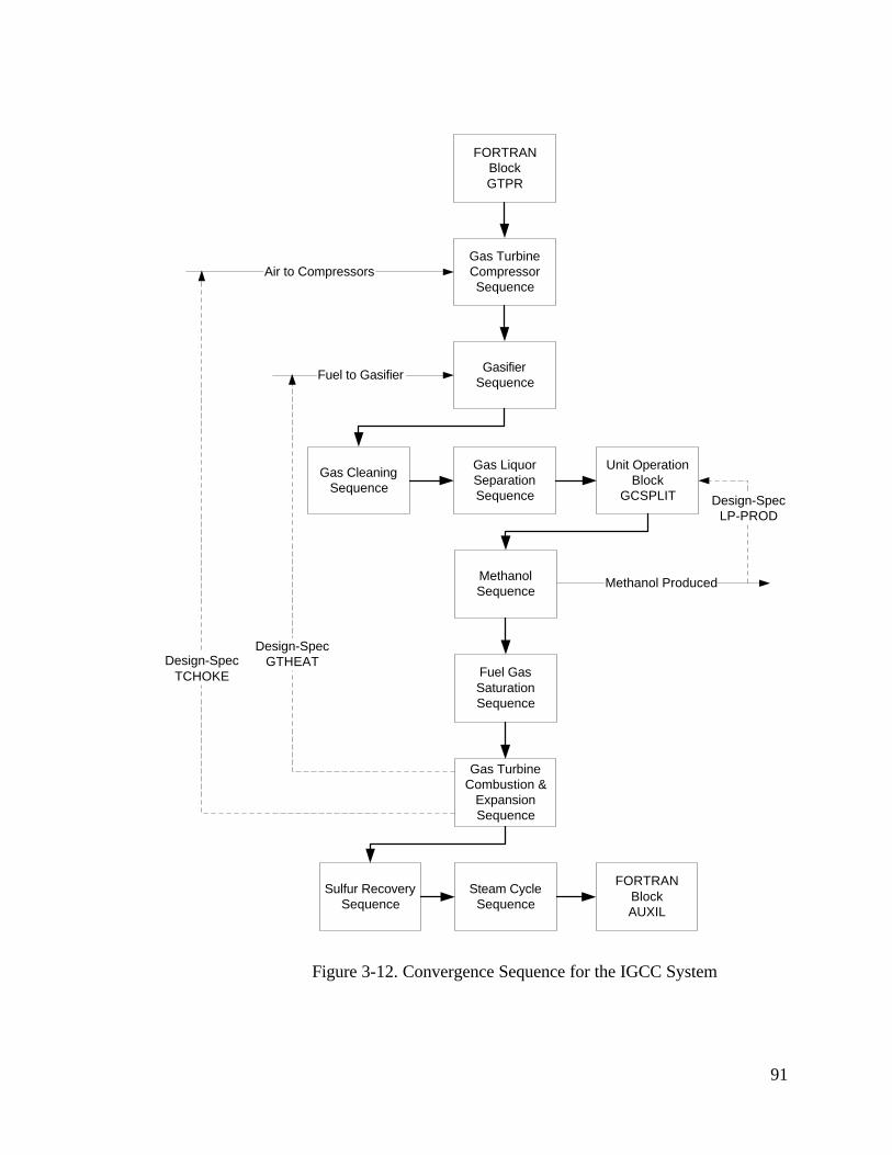
91

Figure 3-12. Convergence Sequence for the IGCC System

FORTRANBlockGTPR

Gas TurbineCompressorSequence

GasifierSequence

Gas CleaningSequence

Gas LiquorSeparationSequence

Unit OperationBlock

GCSPLIT

MethanolSequence

Fuel GasSaturationSequence

Gas TurbineCombustion &

ExpansionSequence

Sulfur RecoverySequence

Steam CycleSequence

FORTRANBlockAUXIL

Air to Compressors

Fuel to Gasifier

Methanol Produced

Design-SpecGTHEATDesign-Spec

TCHOKE

Design-SpecLP-PROD

92

3.5 Environmental Emissions

An objective of this study is to model the emissions of the IGCC system. The

emissions evaluated in this study are NOx, CO, CO2 and SO2. With the exception of

CO2, these gases are regulated under the Clean Air Act of 1990 and the New Source

Performance Standard (NSPS) (Seinfeld and Pandis, 1998). NOx, CO, and SO2 are

regulated under the National Ambient Air Quality Standard (NAAQS) (Seinfeld and

Pandis, 1998). SO2 is a precursor to acid rain and CO has potentially harmful effects on

humans(Seinfeld and Pandis, 1998). CO2 and NOx are believed to contribute to global

warming and are considered greenhouse gases. NOx compounds are also responsible for

ozone layer destruction and photochemical smog (Seinfeld and Pandis, 1998). Other

pollutant emissions modeled in this study are particulate matter and unburned

hydrocarbons.

Compounds of major concern with MSW treatment methods are dioxins and

furans. These are complex, chlorinated compounds that are carcinogenic. However,

results from the Lurgi waste IGCC plant in Germany indicate that the dioxin and furan

emissions were less than 0.01 ng/mn3. These results are less than one-tenth of the strict

German regulation 17.BlmSch V. (Vierrath et. al, 1997). Because the emissions of these

compounds are so low, the production of dioxins and furans are not modeled in the IGCC

system.

3.5.1 NOX Emissions

NOx emissions from the IGCC system are generated as NO and NO2 in the gas

turbine. Due to lack of data, it is difficult to mechanistically model NOx emissions. The

model does not make any meaningful calculation on NOx emissions because these

emissions cannot be estimated based upon simple mass balances, and there are not

emission factors applicable to this particular emission source. The EPRI report by Pechtl

93

et al. (1992) indicates a NOx emission limit of 25 ppmv corrected to 15 percent O2 on a

dry basis.

The default assumptions in the model are that fuel NO are 95 percent by volume

of the fuel NOx and the fraction of NH3 in the syngas that is converted to fuel NOx is

0.90. The reader is directed to Akunuri (1999) for further detail of the formation of NOx

compounds in the gas turbine. For this study, NOx emissions are reported parts ppm

scaled to the emission limit assumed in Pechtl et al. (1992). Reporting NOx emissions in

this manner provides an upper bound for the emissions.

3.5.2 CO and CO2 Emissions

CO is emitted from the IGCC model from the gas turbine. The same problems

arise in modeling CO emissions as do with modeling NOx emissions. There are not any

emission factors applicable to CO emissions for this particular emission source. The CO

emission limit assumed in the EPRI design basis by Pechtl et al. (1992) is 25 ppmv

corrected to 15 percent O2 on a dry basis. In the ASPEN PLUS model, the fraction of CO

oxidized to CO2 in the gas turbine is 0.99985. The CO emissions are reported in ppm

scaled to the design basis assumption, thereby providing an upper limit of CO emissions.

CO2 is emitted from the gas turbine (Stream 183) and the Beavon-Stretford

Section (Stream OFFGAS) and are reported in lb CO2/kWh based on the power supplied

to the power grid.

3.5.3 SO2 Emissions

Most of the sulfur is removed from the syngas prior to combustion by the

Rectisol® process. The default amount of sulfur in the cleaned syngas after the

Rectisol® process is 1 ppm (Eustis and Paffenbarger, 1990). Sulfur is removed before

combustion to prevent corrosion in the gas turbine and so it can be recovered as a

saleable product. The sulfur that is emitted from the gas turbine is a result of combustion

94

of hydrogen sulfide (H2S) to SO2. The amount of SO2 emitted from the gas turbine can

be controlled by adjusting the amount of sulfur removed in the Rectisol® process. Sulfur

is also emitted from the Beavon-Stretford tail gas treatment plant in the form of SO2.

As discussed in Section 2.4, the Rectisol® process has been proven to remove

sulfur to 1 ppm in the clean syngas. However, there is not any data available indicating

the chemical state of the sulfur (e.g., H2S, COS, etc.) for the Rectisol process to achieve

the 1 ppm removal efficiency. Because there is no distinction of what form the sulfur is

in before the Rectisol® process for the reported removal efficiency, an assumption is

made that all sulfur in the crude syngas is H2S.

3.5.4 Particulate Matter and Hydrocarbon Emissions

Particulate matter (PM) and hydrocarbon (HC) emissions are both emitted to the

atmosphere from the HRSG exhaust gas. Both compounds are modeled in this study

using an emission factor assumed in the EPRI study by Pechtl et al. (1992). The

emission factor for PM is 3.0 x 10-6 lb PM/lb flue gas exiting the HRSG and the

hydrocarbon emission factor is 2.6 x 10-6 lb HC/lb flue gas exiting the HRSG. For the

purpose of this study, these emission factors are assumed to be applicable for all of the

fuels used.

95

4.0 CALIBRATION OF THE PERFORMANCE AND EMISSIONS MODEL OF THE COAL FIRED BGL SLAGGING GASIFIER-BASED IGCC SYSTEM

This chapter describes the calibration of individual process areas and the entire

IGCC model. For validation, the model was calibrated to a design study by EPRI of a

BGL gasifier based IGCC system (Pechtl et al., 1992). The gasifier, steam cycle and

complete IGCC system models were calibrated to the EPRI design study. As mentioned

in Section 3.2.5, the gas turbine in the EPRI study does not reflect the latest design of the

General Electric MS70001F. Therefore, the gas turbine was calibrated to a model

developed by Akunuri (1999).

4.1 Calibration of Process Areas

The building of the IGCC system model one process area at a time started with

the three most complex areas of the model: (1) gasification island; (2) gas turbine; and (3)

steam cycle. Each of these process areas were assembled, calibrated and verified

individually before being combined as the IGCC system.

Calibration of the Gas Cooling, Gas Cleaning, Liquor-Gas Separation and fuel gas

saturation models was done based upon the EPRI study by Pechtl et al. (1992). Process

variables such as temperature, pressure, split fractions, etc., were set to the same values

as reported in the studies by Pechtel et al. (1992); and Eustis and Paffenbarger (1990).

The sulfur recovery and LPMEOHTM process models were adapted from previous

models. For the calibration and verification of the sulfur recovery and LPMEOHTM

models, the reader is referred to Stone (1991) and Vaswani (2000), respectively.

96

4.2 Gasification Island

The design basis for the gasification island was adapted from the gasifier of the

IGCC system reported by Pechtl et al. (1992). The fuel used to calibrate the model is a

Pittsburgh #8 coal, as described in Table 3-1. This is the same fuel assumed in the Pechtl

et al. (1992) study. Table 4-1 presents the input assumptions used in calibrating the

gasification island. The input assumptions are based the design study by Pechtl et al.

(1992).

Table 4-1. Input Assumptions for Calibration of the Gasification Island

Coal Feed Rate 287,775 lb/hr Nitrogen for Pressurization 1,653 lb/hr Combustion Zone Temperature 3,357 °F Gasification Zone Temperature 1,300 °F Heat Loss from Gasifier 1.45 % Exiting Syngas Temperature 298 °F Fraction of Carbon in Slag* 1 % Fraction of Sulfur in Slag* 3 % Steam-to-oxygen Molar Ratio 1.036 * From Vierrath (1999)

Table 4-2 presents both an overall mass balance of the calibration and a

comparison with the design basis.

With the exception of the slag, liquid discharge and syngas streams, the model is

calibrated within two percent of the design study. The slag stream, which is the solid

residue from gasification, differs from the model calibration because of the assumption

that three percent of the sulfur from the coal exits in the slag. This assumption is based

on results from Lurgi (Vierrath, 1999). The EPRI study assumed no sulfur exiting in the

slag. ASPEN PLUS calculates more water condensing out of the exiting syngas than the

design basis due to differences in the property data bases used in the two studies. The

difference in property databases results in more liquor from the model, shown in stream

Liquid.

97

Table 4-2. Gasification Island Calibration Comparison EPRI ASPENPLUS Study Model Percent Massflow Massflow Error

Stream (lb/hr) (lb/hr) (%) Inlet Coalfeed 287,775 287,775 0.00% Air 185,210 185,200 -0.01% Steam 93,524 93,546 0.02% Nitrogen 1,653 1,653 0.00% Steam Water 69,631 69,986 0.51% Quench Water 459,244 459,543 0.07% Flux 12,562 12,571 0.08% Steam Quench 1,102 - - Burner Gas 2,346 - - Burner Air 13,098 - - Recycle Tar 13,086 13,084 -0.01% Recycle HC 11,486 11,431 -0.47% TOTAL 1,150,717 1,134,791 -1.38% Exit Liquid 410,964 431,467 4.99% Slag 39,221 42,189 7.57% Syngas 621,906 591,149 -4.95% Jacket Blowdown 636 640 0.63% Jacket Steam 69,631 69,636 0.01% TOTAL 1,142,359 1,135,081 -0.64%

At the lower temperature of the model, more of the water condenses to liquid,

increasing the mass in the liquor stream. The difference in the syngas exit temperature

also contributes to a difference in syngas flowrates.

Table 4-2 shows that there are three streams not modeled in ASPEN PLUS, Steam

Quench, Burner Air, and Burner Fuel. The Burner Air and Burner Fuel streams are air

and fuel streams, respectively, for a stabilization flame in the design study. The Steam

Quench stream is an intermediate-pressure steam used to quench the syngas. This study

did not model the stabilization flame nor the steam quench. Neither of these streams

provides a significant amount of mass or energy to the system and there is a lack of data

on how to relate these streams to changes in the model, e.g., larger plants, different fuels,

etc.

98

It is important to analyze the composition of the crude syngas exiting the gasifier.

Table 4-3 shows the syngas composition for the design basis and for the model. The

model is calibrated by adjusting the approach temperature of the reactions modeled in the

block GASIFXR as described by Equations (3-11) to (3-14). The calibrated approach

temperatures are +520 °F, +460 °F, +150 °F and -360 °F in the block temperature for

reactions (3-11) to (3-14), respectively.

Table 4-3. Crude Syngas Composition Comparison EPRI ASPENPLUS Percent

Component Study (lb/hr) Model (lb/hr) Error CO2 30,764 30,339 -1.38% CO 391,508 392,520 0.26% H2 14,226 14,040 -1.31% CH4 25,423 30,755 20.97% CnHm 6,741 - - H2S/COS 10,015 9,289 -7.25% N2 36,003 29,642 -17.67% H2O 99,213 75,643 -23.76% Oil 5,845 5,844 -0.01% Naphtha 2,142 2,138 -0.19% Phenol 418 290 -30.62% HCN 32 - - Fatty Acids 4 - - NH3 657 649 -1.29% Total Gas 622,994 591,149 -5.11%

Table 4-3 shows relatively large differences in five compounds: CH4; sulfur

containing compounds (H2S/COS); N2; H2O; and Phenol. In the design study,

hydrocarbons are reported as methane and as a general category of CnHm. In the model,

all low molecular weight hydrocarbons are simulated as methane. The mass flow of

methane from the model simulation is similar to the total mass flow of both methane and

other low molecular weight hydrocarbons in the design study. Therefore the difference in

the amount of methane in ASPEN PLUS and the design study mimics the amount of low-

weight hydrocarbons (CnHm) produced in the EPRI study. The lower syngas exit

99

temperature in the model simulation versus the design basis account for the smaller

amount of moisture in the exit syngas, as previously described.

More N2 is introduced in the EPRI study via the burner air required for the

stabilization flame in the gasifier. The excess N2 in the burner air, in the EPRI study,

accounts for the difference between the ASPEN PLUS and EPRI studies. The burner air

stream is not simulated in the ASPEN PLUS model.

In the ASPEN PLUS model, the difference in H2S/COS concentration compared

to the design study is because of a different assumption regarding the amount of sulfur

retained in the slag. The EPRI study assumes that all sulfur in the fuel exits the gasifier

in the syngas. In contrast, in the model three percent of the sulfur in the fuel is retained

in the slag. Another factor in this difference is the fact that all the sulfur in the ASPEN

PLUS model is assumed to be converted to H2S, with no modeling of COS formation.

Because COS has a higher molecular weight than H2S (60 lb/lbmol for COS versus 34

lb/lbmol for H2S), inclusion of COS in the mass balance would produce a greater mass

flow of sulfur containing compounds than reported in the model. However, there is no

data available distinguishing between the ability of the Rectisol® process to remove COS

or H2S, as described in Section 2.4. Therefore, it was determined that the modeling of

COS formation is not necessary in the ASPEN PLUS model.

The overall phenol production from the gasification island in the ASPEN PLUS

model equals that of in the EPRI study. The EPRI study shows 418 lb/hr of phenol in the

crude syngas. The ASPEN PLUS model shows 290 lb/hr in the crude syngas. The

remaining 130 lb/hr of phenol not accounted for in the syngas in the ASPEN PLUS

model is in the liquid discharge, Liquid, shown in Table 4-2. The Fatty Acids and HCN

are not modeled in ASPEN PLUS.

Aside from the previously mentioned differences, the calibration is within 1.50

percent for all other compounds. The 5.11 percent difference in the exiting syngas mass

flow is primarily due to the difference in H2O composition of the syngas. Another reason

100

is due to the additional mass introduced in the EPRI study, via the burner fuel and burner

air for the stabilization flame.

4.3 Gas Turbine

The gas turbine was calibrated to match proprietary specifications of a General

Electric MS7001F gas turbine firing syngas. In order to show the calibration method, the

gas turbine was calibrated to match published specifications for a General Electric

MS7001F firing natural gas. The exhaust gas temperature, simple cycle efficiency and

net power output were used to calibrate the simple cycle efficiency using the method

presented by Akunuri (1999). The three variables used to calibrate the model are: (1)

isentropic efficiency of turbines; (2) isentropic efficiency of compressors; and (3)

reference mass flow of turbine inlet (MREF). Figure 4-1 illustrates the results of the

sensitivity analysis done on the model, showing the published values for a single General

Electric MS7001F with a “+”. The values for a MS7001 gas turbine firing natural gas

include an exhaust gas temperature of 1,116 °F, a simple cycle efficiency of 36.35

percent on a lower heating value basis and a power output of 169.9 MW (Farmer, 1997).

Using a given exhaust gas temperature, Figure 4-1(a) is used to select an

isentropic efficiency for the turbine. A compressor isentropic efficiency is selected from

Figure 4-1(b) to calibrate the simple cycle efficiency. With these two parameters set, an

input assumption, MREF, in the design-spec TCHOKE, is varied to set the power output.

Using a turbine isentropic efficiency of 0.884, a compressor isentropic efficiency of

0.899, and MREF of 3,208,000 lb/hr, the model produces an exhaust gas temperature of

1,115 °F, a simple cycle efficiency of 36.34 percent and a power output of 169.9 MW.

These values are nearly identical to the published data for the gas turbine.

101

Note : ET = Gas Turbine Expander Isentropic Efficiency, “+” = Point of the Calibrated ASPEN PLUS Model Figure 4-1. Plots of (a) Exhaust Gas Temperature, (b) Simple Cycle Efficiency, and (c)

Output Versus Gas Turbine Compressor Isentropic Efficiency

1095

1100

1105

1110

1115

1120

1125

0.88 0.89 0.9 0.91 0.92

Compressor Isentropic Efficiency

Exh

aust

Gas

Tem

p. (

F)

0.88

0.89

0.90

Calibration

ET

35.50%

36.00%

36.50%

37.00%

37.50%

38.00%

0.88 0.89 0.9 0.91 0.92

Compressor Isentropic Efficiency

Sim

ple

Cyc

le E

ffic

ien

cy

0.88

0.89

0.90

Calibration

ET

164.0

166.0

168.0

170.0

172.0

174.0

176.0

178.0

180.0

0.88 0.89 0.9 0.91 0.92

Compressor Isentropic Efficiency

Ou

tpu

t (M

W)

0.88

0.89

0.90

Calibration

ET

102

Using a similar procedure the model was calibrated to the proprietary values

provided by General Electric firing syngas. Using a turbine isentropic efficiency of

0.9285, a compressor isentropic efficiency of 0.7763 and a MREF of 3,484,900 lb/hr, the

ASPEN PLUS model was calibrated to within 0.1 percent of the values provided by

General Electric.

4.4 Steam Cycle

Using an IGCC system design reported by Pechtl et al. (1992), the steam cycle

was developed, based upon a three-pressure level HRSG and a reheat steam turbine-

generator.

For model calibration purposes, all steam and BFW entering and exiting steam

cycle were fixed as input parameters, and the model calculates both the total amount of

water through the cycle and power production. Adjusting the steam quality in the design-

spec STMQUAL varies the power production from the steam turbine. The amount of

BFW supplied to each pressure level is set by adjusting the outlet temperatures of the

heater blocks in the HRSG (e.g. HRSG1, HRSG2, HRSG3, HRSG4), as described in

Section 3.2.6.

Table 4-4 presents a comparison of the design basis and the calibrated model.

The bold numbers in the Massflow, Pressure, and Temperature columns of the ASPEN

PLUS Calibration were fixed as inputs to the model. The model calculates all other

massflows, temperatures, pressures, and states. The Percent Error column compares the

massflows of the design basis and ASPEN PLUS calibration. The results of the

calibration are divided into pressure levels. For each pressure level, the table reports the

total amount of BFW, all steam and BFW interactions with the IGCC system and steam

to the specific turbine stage. In addition to the data for each pressure level, the table

shows all flows into and out of the steam cycle. The Total Blowdown row refers to the

blowdown water from all three boilers while the Total BFW to Steam Cycle is the amount

of water flowing from the deaerator. The Make Up Water is the BFW required by the

103

Table 4-4. Steam Cycle Calibration Comparison

Design Basisa ASPEN PLUS Calibration Massflow Pressure Temp Massflowb Pressure Temp Percent

lb/hr psia °F Statec lb/hr psia °F Statec Errord

High Pressure Level BFW to HP Level 870,252 255 600 L 871,237 251 600 L 0.11% BFW to Process 207,374 254 2,000 L 207,374 254 2,000 L - Hot BFW to Process 109,254 597 1,743 L 109,254 597 1,743 L - HP BFW from Process 316,627 395 2,000 L 316,627 395 2,000 L - Steam to HP Turbine 861,635 1,000 1,465 SH 862,612 1,000 1,465 SH 0.11%

Intermediate Pressure Level BFW to IP Level 221,577 251 600 L 227,345 251 600 L 2.60% IP BFW to Process 90,643 252 600 L 90,643 252 600 L - IP Steam to Process 108,578 716 508 SH 108,578 716 508 SH - Steam to IP Turbine 882,694 1,000 469 SH 883,473 1,000 469 SH 0.09%

Low Pressure Level BFW to LP Level 212,161 252 600 L 211,987 251 600 L -0.08% LP Steam to Process 44,709 339 116 SAT 44,709 339 116 SAT - Steam to LP Turbine 982,964 381 29 SH 979,249 370 29 SH -0.38%

Total Blowdown 10,968 30 250 L 10,978 30 250 L 0.09% Total BFW to Steam Cycle 1,311,072 250 30 L 1,310,570 250 30 L -0.04% Make Up Water 192,926 60 25 L 192,936 60 25 L 0.01% Condensate Return 61,973 116 339 L 61,973 116 339 L -

Power (MW) 160.1 160.1 0.00%

a Design Basis adopted from Pechtl et al.,1992 b Numbers in BOLD indicate input parameters c L = Liquid; SAT = Saturated Steam; SH = Superheated Steam d Percent Error of Massflow

103

104

steam cycle to replace the water consumed in the steam cycle or process. Finally,

Condensate Return is the total amount of condensate returned from steam being cooled in

other areas in the plant. The table also shows the total power production from the steam

cycle.

With the exception of the BFW to the intermediate-pressure level all of the

massflows in Table 4-4 are within 0.40 percent of the design basis, thereby verifying the

model. The BFW provided to the intermediate-pressure level is 2.60 percent higher than

the design study. The percent error can be more closely calibrated by adjusting the outlet

temperature of the unit operation block, HRSG2. However, because the BFW provided

to the intermediate-pressure level is an interior stream it does not reflect the in the models

overall performance, such as power production. Therefore, an error of 2.60 percent for

the BFW fed to the intermediate-pressure level is within acceptable tolerance.

4.5 IGCC System

The EPRI study by Pechtl et al. (1992) was used as the design basis for

calibrating the overall IGCC system model. Since the design basis does not incorporate a

methanol plant, it was taken out of the IGCC model for calibration purposes. Both the

design basis and ASPEN PLUS model employ two General Electric MS7001F turbines,

governing the size of the plant. As mentioned in Section 3.1, the gas turbine has a

pressure ratio of 15.5 and a firing temperature of 2,350 °F in the ASPEN PLUS model,

while the pressure ratio and firing temperature are not reported for the EPRI design basis.

Table 4-5 compares the results of the calibration to the design study. Table 4-5

shows the auxiliary power loads for each section, the amount of power generated and key

massflow rates. A key difference in the two designs is the gas cleaning process used in

the ASPEN PLUS model, the Rectisol® process. As mentioned in Section 2.4.1, the

Rectisol® process has much greater steam and electricity demands than other gas

cleaning processes. Table 4-5 indicates this by the 124 percent increase in power demand

for the Acid Gas Removal Section when comparing the Rectisol® process to the Purisol

105

Table 4-5. Comparison of IGCC System Calibration Results Power (MW) Percent Mass Flow Rates Mass Flow (#/hr) Percent

Auxillary Loads ASPEN PLUS EPRI Error (%) ASPEN PLUS EPRI Error (%) Oxygen Plant 28.50 32.10 -11.21% To Gasifier Fuel 314,540 318,090 -1.12% Gasification Island 1.01 0.93 9.60% Oxygen 181,368 183,012 -0.90% Liquor Separation 0.66 0.65 1.72% Steam 106,159 106,979 -0.77% BFW Treatment 0.61 0.62 -2.09% Quench Water 513,176 464,650 10.44% Fuel Gas Satuartion 0.13 0.12 2.98% Crude Syngas 648,671 642,236 1.00% Beavon-Stretford Tailgas 0.43 N/A - Clean Syngas to Saturator 511,159 535,483 -4.54% Acid Gas Removal 7.12 3.18 123.49% Saturated Syngas 943,723 988,261 -4.51% Coal Receive & Stor and Prep 1.81 1.79 1.01% Air to Gas Turbine 6,936,730 6,617,339 4.83% Liquor Treatment 0.16 0.18 -9.17% Fired Fuel Mixture in Gas Turb. 6,631,940 Not Available - Claus Plant 0.20 w/Acid Gas - Overall Consumption of Water 510,921 529,761 -3.56% Power Island 3.86 3.78 2.14% Production of Sulfur 9,916 9,892 0.24% General Facilities* 3.65 3.68 -0.90% Slag Production 46,113 49,796 -7.40% TOTAL AUX LOADS (MW) 48.13 48.33 -0.41% Saturation Water 394,417 396,346 -0.49% Steam for Sat. Heating 297,067 326,634 -9.05% POWER GENERATION (MW)

Gas Turbines 383.9 384.0 -0.04% Steam Turbines 131.6 135.1 -2.56% ENERGY INPUT MMBTU/hr MMBTU/hr**

Gross Power Generated 515.5 519.1 -0.69% HHV Basis 3,885 3,964 -2.00% Auxiliary Load 48.1 48.3 -0.41% LHV Basis 3,728 3,804 -2.00%

Power to Grid 467.4 470.8 -0.72% OVERALL THERMAL EFF. HEAT RATE BTU/kWh BTU/kWh

HHV BASIS 41.1% 40.5% 1.36% HHV 8,312 8,420 -1.29% LHV BASIS 42.8% 42.2% 1.38% LHV 7,976 8,080 -1.29%

*In EPRI, General Facilities includes: General Facilities, Sewage & Effluent Treatment, Raw Water Supply & Treat and Cooling Water ** EPRI includes heat from Bitumen and coal

105

106

process used in the design report. The Rectisol® plant also uses more steam than the

Purisol process of the design study, lowering power generation from the steam cycle. As

steam requirements rise, less mass flows through the steam turbine, resulting in a lower

power production.

The quench water requirement predicted in the ASPEN PLUS model is 10 percent

higher than the amount reported in the design basis. The quench requirement is over-

predicted in the model because of lack of data regarding the quench vessel’s outlet

temperature in the design basis. More quench water in the syngas translates to a higher

crude syngas flow rate exiting the gasification island in the model. However, after the

syngas is dried and cleaned, i.e., Clean Syngas to Saturator, the ASPEN PLUS model

predicts roughly 5 percent less massflow than the design basis. This is roughly the same

error in the calibration of the gasification island, as described in Section 4.2. The main

difference, from a massflow perspective, between the Crude Syngas and the Clean

Syngas to Saturator is the H2O contained in the syngas. The high massflow of the Crude

Syngas is due to the over-predicted amount of Quench Water.

Because there is less syngas proceeding to the Saturation area in the ASPEN

PLUS model than the design basis, and both cases saturate the syngas to roughly 45

mass-percent water, there is less saturated syngas exiting the Saturation area.

The internal flows of the gas turbine used in the design basis are difficult to

compare with the gas turbine used in the ASPEN PLUS model. The pressure ratio, firing

temperature and other key calibration data requirements are not known for the design

basis. The key parameter for the gas turbine is the amount of power produced. The

model is within 0.5 percent of the design basis.

Table 4-5 shows a 1.12 percent decrease in coal usage by the model compared to

the design basis, which may be attributed, in part, to the Rectisol® process. The

Rectisol® process removes a significant amount of CO2 from the crude syngas. The

Rectisol® process removes all but two percent of the CO2 from the crude syngas, which

107

increases the heating value of the fuel and therefore lowers the gas turbine’s syngas

requirement on a massflow basis. Because less syngas is required, less coal is required.

The model uses 9.05 percent less steam for heating the fuel gas saturation area

compared to the design study. In the model, the primary source of heat for the fuel gas

saturation section comes from the water circulating between the fuel gas saturation

section and the Gas Cooling section. This water is used to transport heat from the syngas

in the Gas Cooling section to the fuel gas saturation process area. The design-spec

GCSATH2O determines the amount of water in the Gas Cooling Section. Whatever heat

duty not provided by the Gas Cooling water is made up by steam from the steam cycle.

More crude syngas in the ASPEN PLUS model results in more cooling water circulating

between the Gas Cooling and fuel gas saturation sections. Since more heat is being

provided from the circulating water, less steam is required from the steam cycle.

In total, the model predicts an increase of 0.6 percent in overall thermal efficiency

over the design basis. The model predicts 3,350 lb coal/hr, 79 MMBTU/hr, less than the

design basis while producing only 2.4 MW less power. There is 1.12 percent less coal

fueling the model for only 0.72 percent less power produced than the design basis,

explaining the increase in thermal efficiency of the model over the design basis.

108

5.0 SENSITIVITY ANALYSIS OF THE PERFORMANCE AND EMISSIONS MODEL OF THE COAL FIRED BGL SLAGGING GASIFIER-BASED IGCC SYSTEM

After the model has been verified, a sensitivity analysis was performed. In the

sensitivity analysis, the effects of changes in selected individual model inputs were

evaluated with respect to changes in selected model outputs. The objectives of the

sensitivity analyses were: (1) to further verify the adequacy of the model by observing

and evaluating how well the model responds to changes in inputs; and (2) to aid in

identifying key performance and design variables that have the most significant impact

on system performance. This chapter presents the descriptions and results of sensitivity

analyses performed on the gasifier, steam cycle and the entire IGCC model. A sensitivity

analysis was also performed on the gas turbine as discussed in Section 4.3.

5.1 Gasification Area

As part of the sensitivity analysis for the gasifier, three parameters in the

gasification island were varied: (1) the combustion zone temperature; (2) the steam-to-

oxygen ratio; and (3) the gasification zone temperature. The range of variation for each

parameter included the calibrated value. Four model outputs were evaluated in all three

sensitivity analyses: (1) the power production by the Steam Turbine; (2) the power

production of the gas turbines; (3) the auxiliary power load; and (4) the overall net

efficiency and power produced from the IGCC system.

5.1.1 Combustion Zone Temperature

The combustion zone is a crucial zone of the gasifier because it provides heat to

the rest of the gasifier vessel and determines the state (i.e., solid or liquid) the non-

combustible material exits the vessel. The combustion zone temperature of the gasifier

was varied over a range of 3,300 °F to 3,600 °F. The calibrated temperature is 3,357 °F.

The minimum temperature for the model is 3,300 °F because below this temperature the

109

carbon in the fuel is not fully oxidized before leaving the gasification island. Above

3,600 °F, all the carbon in the fuel is combusted before leaving the combustion zone

creating a combustor instead of a gasifier.

The amount of oxidant and steam introduced to the gasifier is determined based upon the

combustion zone temperature. Figure 5-1 illustrates the variation in steam and oxidant

mass flowrates with respect to variation in the combustion zone temperature. Figure 5-1

shows that as the combustion temperature increases, the amount of oxygen, and therefore

steam, increases as well. As more oxygen is available, more carbon is combusted;

thereby giving off more heat. The more heat that is given off by the combustion of

carbon, the more the temperature increases.

Figure 5-1. Plot of Molar Oxidant and Steam Flowrates to Gasifier versus Gasifier Combustion Zone Temperature

Table 5-1 displays the variation of crude syngas composition and heating value

with respect to variation in the gasifier combustion zone temperature. The row labeled

5000

5500

6000

6500

7000

7500

3250 3300 3350 3400 3450 3500 3550 3600 3650Combustion Zone Temperature (°F)

Mol

ar F

low

rate

(lb

mol

/hr)

Oxidant

Steam

110

“Other” includes the NH3, Phenol, Naphtha and Oil compounds. Table 5-1 shows

decreasing amounts of CH4, CO and “Other” compounds in the crude syngas as the

combustion temperature and the amounts of CO2 and H2 simultaneously increase. The

amount of H2 increases as a result of the higher steam input with increased combustion

zone temperature. The CO2 content of the syngas increases with combustion zone

temperature as a result of more oxygen in the gasifier and therefore more complete

combustion. More of the carbon in the fuel is fully oxidized to CO2 as the combustion

zone temperature increases, resulting in less carbon for CH4 and CO formation.

As combustible components, CO and CH4 are major contributors to the heating

value of the syngas. An increase in combustion zone temperature results in a lower

heating value for the syngas, as shown in Table 5-1, due to the drop in CH4 and CO

compositions and simultaneous increase in CO2 composition in the syngas. The lower

heating value of the syngas requires more syngas production to satisfy the gas turbine

fuel demands. Crude syngas production therefore increases with combustion zone

temperature.

Table 5-1. Variation in Crude Syngas Composition with Respect to Variation in Combustion Zone Temperature

Combustion Zone Temperature (°F) Description 3300 3400 3500 3600

Syngas Composition, mole% H2 23.0% 24.0% 24.8% 25.4% N2 1.4% 1.5% 1.5% 1.5% H2O 17.8% 17.8% 17.8% 17.8% H2S 0.9% 0.9% 0.9% 0.9% CH4 7.2% 6.1% 5.1% 4.2% CO 47.2% 46.8% 46.8% 46.2% CO2 2.1% 2.6% 3.2% 3.8% Other* 1.8% 0.3% 0.2% 0.2% Syngas HHV (BTU/lb) 6030 5860 5692 5524 Coal Flow (lb/hr) 311,903 316,500 322,145 328,192

* Other - includes NH3, Phenol, Naphtha and Oil compounds

111

Table 5-2 displays the amount of power produced from the Gas and Steam

Turbines, the auxiliary power loads and the net efficiency of the IGCC system for various

combustion zone temperatures.

Table 5-2. Gas and Steam Turbine Power Generation, Auxiliary Power Load and Overall Net Efficiency for various Gasifier Combustion Zone Temperatures

Power (MW) Combustion Zone Temperature (°F)

Gas Turbine Steam Turbine Auxiliary

Load Net Power Produced

Net Efficiency

3300 383.3 128.3 46.8 464.8 39.3 3400 384.7 131.0 49.9 465.7 38.8 3500 385.9 134.2 53.2 466.9 38.3 3600 387.0 138.3 56.7 468.6 37.7

As discussed in Section 2.6, the lower the heating value of a fuel, the more power

produced from the gas turbine. Table 5-2 shows the expected increase in power from the

gas turbine, resulting from the decrease in syngas heating value with increasing

combustion zone temperature. Due to higher oxidant demand and increased syngas

production associated with rising combustion zone temperature, the auxiliary power load

also increased. Almost every process area experienced an increase in auxiliary load due

to the increase in syngas production, but the load that affected the overall load the most is

the oxygen plant. This load increased due to the higher demand for oxygen.

A significant use of steam from the steam cycle is from the fuel gas saturation

area. As discussed in Section 4.5, more syngas massflow through the Gas Cleaning

section results in less steam to the fuel gas saturation area. Lower steam demands in the

steam cycle, result in greater power production by the Steam Turbine. The net power

production varies only 3.8 MW as combustion zone temperature is increased because the

extra power produced from the Steam and gas turbines is balanced by increased auxiliary

power demands. However, the net efficiency decreases from 39.3 percent at a

combustion zone temperature 3,300 °F to 37.7 percent at a combustion zone temperature

of 3,600 °F because of increased fuel consumption, as shown in Table 5-1.

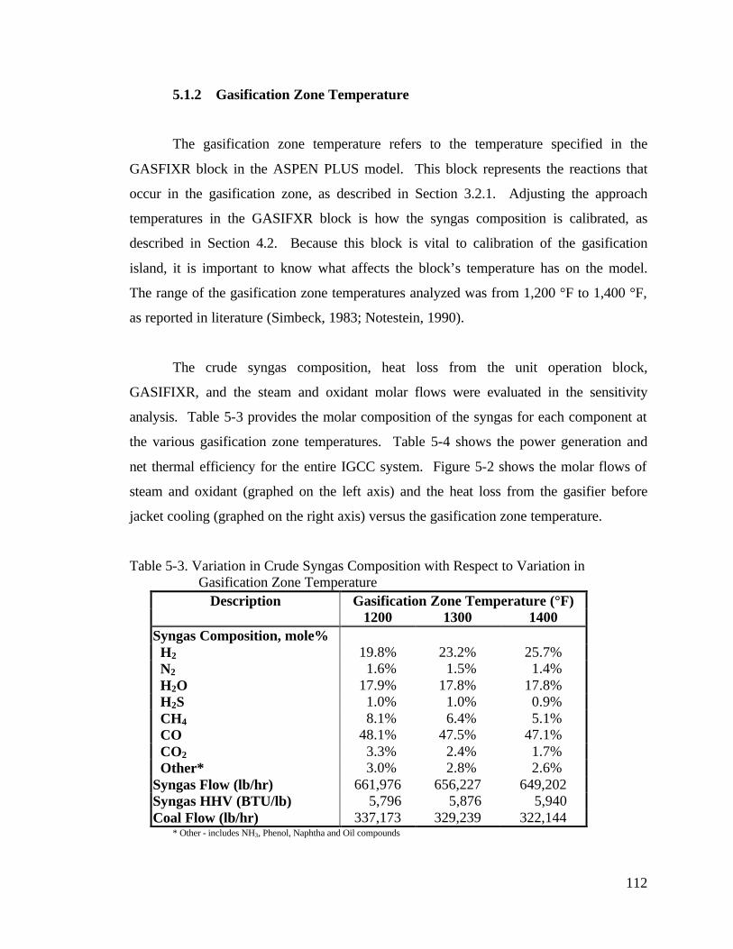
112

5.1.2 Gasification Zone Temperature

The gasification zone temperature refers to the temperature specified in the

GASFIXR block in the ASPEN PLUS model. This block represents the reactions that

occur in the gasification zone, as described in Section 3.2.1. Adjusting the approach

temperatures in the GASIFXR block is how the syngas composition is calibrated, as

described in Section 4.2. Because this block is vital to calibration of the gasification

island, it is important to know what affects the block’s temperature has on the model.

The range of the gasification zone temperatures analyzed was from 1,200 °F to 1,400 °F,

as reported in literature (Simbeck, 1983; Notestein, 1990).

The crude syngas composition, heat loss from the unit operation block,

GASIFIXR, and the steam and oxidant molar flows were evaluated in the sensitivity

analysis. Table 5-3 provides the molar composition of the syngas for each component at

the various gasification zone temperatures. Table 5-4 shows the power generation and

net thermal efficiency for the entire IGCC system. Figure 5-2 shows the molar flows of

steam and oxidant (graphed on the left axis) and the heat loss from the gasifier before

jacket cooling (graphed on the right axis) versus the gasification zone temperature.

Table 5-3. Variation in Crude Syngas Composition with Respect to Variation in Gasification Zone Temperature

Description Gasification Zone Temperature (°F) 1200 1300 1400

Syngas Composition, mole% H2 19.8% 23.2% 25.7% N2 1.6% 1.5% 1.4% H2O 17.9% 17.8% 17.8% H2S 1.0% 1.0% 0.9% CH4 8.1% 6.4% 5.1% CO 48.1% 47.5% 47.1% CO2 3.3% 2.4% 1.7% Other* 3.0% 2.8% 2.6% Syngas Flow (lb/hr) 661,976 656,227 649,202 Syngas HHV (BTU/lb) 5,796 5,876 5,940 Coal Flow (lb/hr) 337,173 329,239 322,144

* Other - includes NH3, Phenol, Naphtha and Oil compounds

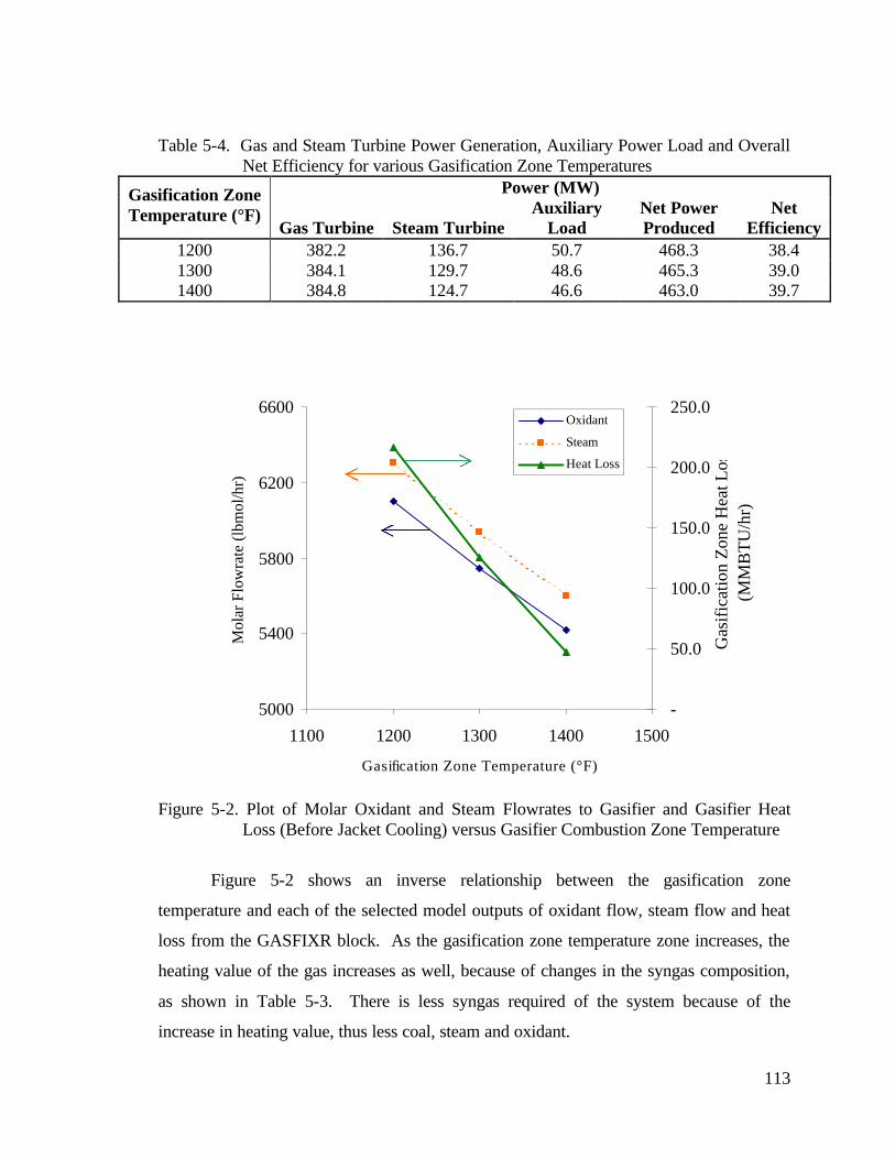
113

Table 5-4. Gas and Steam Turbine Power Generation, Auxiliary Power Load and Overall Net Efficiency for various Gasification Zone Temperatures

Power (MW) Gasification Zone Temperature (°F)

Gas Turbine Steam Turbine Auxiliary

Load Net Power Produced

Net Efficiency

1200 382.2 136.7 50.7 468.3 38.4 1300 384.1 129.7 48.6 465.3 39.0 1400 384.8 124.7 46.6 463.0 39.7

Figure 5-2. Plot of Molar Oxidant and Steam Flowrates to Gasifier and Gasifier Heat Loss (Before Jacket Cooling) versus Gasifier Combustion Zone Temperature

Figure 5-2 shows an inverse relationship between the gasification zone

temperature and each of the selected model outputs of oxidant flow, steam flow and heat

loss from the GASFIXR block. As the gasification zone temperature zone increases, the

heating value of the gas increases as well, because of changes in the syngas composition,

as shown in Table 5-3. There is less syngas required of the system because of the

increase in heating value, thus less coal, steam and oxidant.

5000

5400

5800

6200

6600

1100 1200 1300 1400 1500

Gasification Zone Temperature (°F)

Mol

ar F

low

rate

(lb

mol

/hr)

-

50.0

100.0

150.0

200.0

250.0

Gas

ific

atio

n Z

one

Hea

t Los

s (M

MB

TU

/hr)

Oxidant

Steam

Heat Loss

114

Block temperature increases result in an increased energy demand from the

GASIFXR. Heat streams from the unit operation blocks GCCOMB and BRKDWN

provide the energy utilized by the unit operation block GASIFXR. The heat not

consumed by the GASIFXR block is excess heat, or the heat loss from the block. At high

temperature the GASIFXR block uses more energy resulting in less excess heat. This

heat is recovered to make low-pressure steam.

Table 5-3 shows that raising the temperature of the gasification zone results in a

decrease in the amount of CO, CO2, CH4 and “Other” components and an increase in H2

content. Because the CH4 formation, Equation 3-13, is exothermic (Tchobanoglous et.

al, 1993), it is expected that the methane composition in the syngas would drop with an

increase in syngas temperature. However, there is a lot of uncertainty in trying to make a

prediction for the compositions for H2, CO and CO2 in the syngas without utilizing the

model. Equations 3-11 through 3-14 show these three compounds are products and

reactants of exothermic and endothermic reactions. Yet, Table 5-3 shows an increase of

the H2 composition by 5.9 percent and a decrease of CO by 1.0 percent, CH4 by 3.0

percent and the CO2 composition was almost cut in half.

Shown in Table 5-4, the increase in gasification zone temperature improves the

overall thermal efficiency of the plant. The increase in net efficiency is a result of the

increase in the syngas heating value. A higher syngas heating value results in less

syngas requirement and a subsequent decrease in coal throughput.

The power production from the Gas turbine remains fairly constant over the range

of gasification zone temperatures. However, increasing gasification zone temperature

results in a drop in both the steam turbine power production and auxiliary loads. As

discussed in Section 5.1.1, as more syngas flow through the Gas Cooling area, the steam

cycle produces more power. In this case, the opposite scenario is displayed. There is less

syngas through the system, resulting in a decrease in steam turbine power generation.

Subsequently, the decrease in syngas production results in decreases in auxiliary loads.

115

5.1.3 Steam-to-Oxygen Ratio

The steam-to-oxygen ratio is one of the only controlled variables in gasification

that can be used to directly manipulate the syngas composition in an actual gasifier, yet it

is one of the most uncertain parameters in gasification. Most values found in the

literature are either rough estimates or withheld as proprietary information. A sensitivity

analysis was performed varying the steam-to-oxygen ratio to better understand how it

affects the performance of the model. The ratio was varied from 0.95 to 1.10, covering

the ratios for BGL Gasifiers firing bituminous and sub-bituminous coals that are reported

in the literature (Hebden and Stroud, 1981).

Figure 5-3 shows the HHV of the syngas (plotted on right axis) and the steam and

oxygen molar flows (plotted on the left axis) versus the steam-to-oxygen ratio. Figure 5-

3, shows that the oxidant flow remains fairly constant and the steam flow increases as the

steam-to-oxygen ratio increases. The steam flow increases as a direct result of the

increase in the steam-to-oxygen ratio. Steam acts as a thermal diluent in the gasifier.

The temperature of the gasifier remains constant over the range of steam-to-oxygen

ratios, resulting in a slight increase in oxidant to overcome the temperature lowering

action of the steam.

Figure 5-3 shows that the heating value of the syngas peaks at a steam-to-oxygen

ratio of 0.98. The heating value drops as the steam-to-oxygen ratio rises. A similar trend

appears with the steam and oxygen supplied to the gasifier. However, Table 5-5 indicates

maximum net plant efficiency at a steam-to-oxygen ratio of 1.01.Table 5-5 also indicates

decreases in the Steam Turbine power production, net power production and auxiliary

loads, when the steam-to-oxygen ratio increases. Table 5-6 shows an increase in H2 and

CO2 composition in the crude syngas as the steam-to-oxygen ratio increases. Also shown

in Table 5-6 is the drop in CO and CH4 in the crude syngas with increasing steam-to-

oxygen ratio.

116

Figure 5-3. Plot of Molar Oxidant and Steam Flowrates to Gasifier and Crude Syngas Higher Heating Value versus Molar Steam-to-oxygen Ratio

Table 5-5. Gas and Steam Turbine Power Generation, Auxiliary Power Load and Overall Net Efficiency for various Steam-to-oxygen Molar Ratios

Power (MW) Steam-to-oxygen Molar Ratio

Gas Turbine Steam Turbine Auxiliary

Load Net Power Produced

Net Efficiency

0.95 383.7 131.8 48.0 467.4 38.6 0.98 383.7 130.9 47.7 466.9 39.1 1.01 383.8 130.6 47.8 466.5 39.2 1.04 384.0 130.3 48.1 466.2 39.1 1.07 384.1 130.1 48.4 465.7 39.1 1.10 384.1 129.5 48.7 464.9 39.0

5000

5200

5400

5600

5800

6000

6200

0.92 0.96 1 1.04 1.08 1.12Steam to O xygen Molar Ratio

Mol

ar F

low

rate

(lb

mol

/hr)

300.0

303.0

306.0

309.0

Hig

her

Hea

ting

Val

ue o

f Syn

gas

(BT

U/S

CF

)

Oxidant

Steam

HHV of Syngas

117

Table 5-6. Crude Syngas Composition Variance with Steam-to-oxygen Ratio Description Steam-to-oxygen Ratio

0.95 0.98 1.01 1.04 1.07 1.10 Syngas Composition, mole% 21.9% 21.9% 22.2% 22.6% 23.0% 23.3% H2 1.5% 1.5% 1.5% 1.5% 1.5% 1.5% N2 17.8% 17.8% 17.8% 17.8% 17.8% 17.8% H2O 1.0% 1.0% 1.0% 1.0% 1.0% 1.0% H2S 7.1% 7.1% 7.0% 6.7% 6.5% 6.3% CH4 48.3% 48.3% 48.1% 47.8% 47.6% 47.4% CO 2.1% 2.1% 2.1% 2.3% 2.4% 2.5% CO2 2.9% 2.9% 2.9% 2.8% 2.8% 2.8% Syngas Flow (lb/hr) 648,115 647,518 649,201 652,216 655,021 659,251 Syngas HHV (BTU/lb) 5,933 5,936 5,922 5,900 5,878 5,856 Coal Flow (lb/hr) 334,916 330,220 328,850 329,130 329,330 329,260

*Other - includes NH3, Phenol, Naphtha and Oil compounds

5.2 Steam Cycle

In the stand-alone steam cycle (i.e., the steam cycle by itself with no connection

to the rest of the IGCC system), the steam and BFW contacts with the IGCC system are

specified as inputs. It is these inputs that are varied for the sensitivity analysis. The

sensitivity analysis was done to simulate an increase/decrease of the steam requirement of

the IGCC system while observing the reaction of the steam cycle.

As described in Section 3.2.6, there are three pressure levels of steam generation

in the steam cycle: (1) low-pressure; (2) intermediate-pressure; and (3) high-pressure.

The sensitivity analysis for the steam cycle was performed by varying the steam and

BFW demand at each pressure level by twenty percent. The variables were varied by

twenty percent to ensure the model could handle a wide range of steam demands.

For each sensitivity analysis at each pressure level, a mass balance had to be

maintained. If the total mass exiting the pressure-level was increased by 20,000 lb/hr,

then 20,000 lb/hr is going to return to the steam cycle. However, it may not be as

obvious where the mass returns to the steam cycle, since the steam or BFW may not

return in the same pressure level or state that it exited. For example, the low-pressure

level sensitivity analysis varied the LP Steam to Process by twenty percent. The total

118

amount of LP Steam to Process in the calibrated case is 44,709 lb/hr and is varied by plu

or minus 8,941 lb/hr (44,709 * 0.20 = 8,941) for the sensitivity analysis. This mass is

returned to the steam cycle as process condensate; however, the stream Condensate

Return contains condensate from both low-pressure and intermediate-pressure steam

flows. Therefore, the Condensate Return stream was varied by only 8,941 lb/hr (e.g., in

the High column of Table 5-4; 61,973 + 8,941 = 70,914). Similar calculations were

carried out in the intermediate- and high-pressure level steam cycle analyses.

5.2.1 Low-Pressure Level

The low-pressure level sensitivity analysis was performed by varying the low-

pressure steam to the process by twenty percent. Low-pressure steam is used in the fuel

gas saturation area, sulfur recovery area, Rectisol® process and LPMEOHTM plant. A

description of the sensitivity analysis on the low-pressure level is provided in the

previous Section.

Table 5-7 shows the results of the low-pressure sensitivity analysis of the steam

cycle. The numbers in bold indicate the parameters that were varied for the analysis.

The results from the calibrated model are provided in the “Model Calibration” column.

The results for the analysis of twenty percent greater than the calibrated model are in the

“High” column; the results for twenty percent less than the calibrated model are in the

“Low” column. The table also provides the percent error between each case study and

the calibrated model.

Table 5-7 shows that by adjusting the low-pressure level demand, the overall

power produced from the steam cycle changes by 0.4 percent. As the amount of low-

pressure steam demanded by the IGCC system increases, less mass is available for the

Steam Turbine. In this case, the amount of steam in the Low Pressure Steam Turbine

119

Table 5-7. Steam Cycle Low-Pressure Sensitivity Analysis

changes by 0.6 percent. Lower mass flow through the turbine results in less power

production. The amount of BFW to the intermediate-pressure level changed by 0.5

percent as the low-pressure steam demand of the IGCC system varied. The intermediate-

pressure BFW changes because it is used to create low-pressure steam, as described in

Section 3.2.6.2.

Model Low-Pressure Level Sensitivity Analysisa Calibration Highc Percent Lowd Percent High-Pressure Level lb/hr lb/hr Error lb/hr Error Stateb

Boiler Feed Water (BFW) to HP Level 871,237 871,241 0.0% 871,241 0.0% L BFW to Process 207,374 207,374 0.0% 207,374 0.0% L Hot BFW to Process 109,254 109,254 0.0% 109,234 0.0% L HP BFW from Process 316,628 316,628 0.0% 316,628 0.0% L Steam to HP Turbine 862,612 862,616 0.0% 862,616 0.0% SH Intermediate-Pressure Level

BFW to IP Level 227,345 228,539 0.5% 226,151 -0.5% L IP BFW to Process 90,643 90,643 0.0% 90,643 0.0% L IP Steam to Process 108,578 108578 0.0% 108,578 0.0% SH Steam to IP Turbine 883,473 883,478 0.0% 883,478 0.0% SH Low-Pressure Level BFW to LP Level 211,987 211,985 0.0% 211,985 0.0% L LP Steam to Process 44,709 53,650 20.0% 35,767 -20.0% SAT Steam to LP Turbine 979,249 973,478 -0.6% 985,024 0.6% SH Total Blowdown 10,978 10,979 0.0% 10,979 0.0% L Steam to Deaerator 76,411 74,436 -2.6% 78,386 2.6% SAT Total BFW to Steam Cycle 1,310,570 1,311,766 0.1% 1,309,379 -0.1% L Make Up Water 192,936 192,936 0.0% 192,936 0.0% L Condensate Return 61,973 70,914 14.4% 53,031 -14.4% L Power (MW) 160.1 159.4 -0.4% 160.7 0.4%

a Numbers in BOLD indicate parameters of sensitivity analysis b L = Liquid; SAT = Saturated Steam; SH = Superheated Steam c High = Set LP Steam to Process and 44,709 lb/hr of Condensate Return to +20% of Calibration d Low = Set LP Steam to Process and 44,709 lb/hr of Condensate Return to -20% of Calibration

120

5.2.2 Intermediate-Pressure Level

The intermediate-pressure level sensitivity analysis was done in two parts: (1)

varying the intermediate-pressure steam; and (2) varying the intermediate-pressure BFW.

Table 5-8 shows the results of both analyses. For the intermediate-pressure level BFW

analysis, the IP BFW to Process was varied by twenty percent. The intermediate-

pressure BFW sent to the IGCC Process generates low-pressure steam so, the amount of

low-pressure steam was inversely adjusted to maintain the mass balance. The

Condensate Return was also varied by 465 lb/hr (twenty percent of the amount of

intermediate-pressure BFW that is returned to the steam cycle) to maintain the mass

balance.

The intermediate-pressure steam was varied by plus or minus twenty percent as

part of the steam cycle analysis. Out of the 61,973 lb/hr of Condensate Return, 14,105

lb/hr is from the intermediate-pressure steam, which was varied by twenty percent as part

of the analysis. The majority of the intermediate-pressure steam is consumed in the

gasifier.

Table 5-8 shows that an increase in intermediate-pressure BFW raises the power

production of the Steam Turbine. The boost in power is a result of the consequential

decrease in low-pressure steam demand of the steam cycle. With less low-pressure steam

being demanded of the steam cycle, then there is more mass in the Steam Turbine, which

raises power production.

The steam cycle also adjusted to the varying intermediate-pressure BFW demand

by calculating more BFW in the steam cycle, splitting more of the BFW to the

intermediate-pressure level, and increasing the amount of Make Up Water required to

maintain an overall mass balance.

121

Table 5-8. Steam Cycle Intermediate-Pressure Sensitivity Analysis Intermediate-Pressure Level Sensitivity Analysisa Model IP BFW IP Steam Calibration Highb Percent Lowc Percent Highd Percent Lowe Percent

High-Pressure Level lb/hr lb/hr Error lb/hr Error lb/hr Error lb/hr Error Statef

Boiler Feed Water (BFW) to Process 871,237 871,218 0.0% 871,036 0.0% 874,650 0.4% 867,833 -0.4% L BFW to Process 207,374 207,374 0.0% 207,374 0.0% 207,374 0.0% 207,374 0.0% L Hot BFW to Process 109,254 109,254 0.0% 109,254 0.0% 109,254 0.0% 109,254 0.0% L HP BFW from Process 316,628 316,628 0.0% 316,628 0.0% 316,628 0.0% 316,628 0.0% L Steam to HP Turbine 862,612 862,593 0.0% 862,412 0.0% 865,137 0.3% 859,242 -0.4% SH Intermediate-Pressure Level BFW to IP Level 227,345 244,278 7.4% 210,396 -7.5% 227,345 0.0% 227,345 0.0% L IP BFW to Process 90,643 108,771 20.0% 72,514 -20.0% 90,643 0.0% 90,643 0.0% L IP Steam to Process 108,578 108,578 0.0% 108,578 0.0% 130,293 20.0% 86,862 -20.0% SH Steam to IP Turbine 883,473 883,454 0.0% 883,274 0.0% 865,137 -2.1% 901,819 2.1% SH Low-Pressure Level BFW to LP Level 211,987 211,995 0.0% 212,082 0.0% 210,411 -0.7% 213,559 0.7% L LP Steam to Process 44,709 35,767 -20.0% 53,650 20.0% 44,708 0.0% 44,708 0.0% SAT Steam to LP Turbine 979,249 984,343 0.5% 974,042 -0.5% 959,560 -2.0% 998,943 2.0% SH Total Blowdown 10,978 10,978 0.0% 10,977 0.0% 11,005 0.2% 10,953 -0.2% L Steam to Deaerator 76,411 79,053 3.5% 73,751 -3.5% 76,196 -0.3% 76,627 0.3% SAT Total BFW to Steam Cycle 1,310,570 1,327,490 1.3% 1,293,514 -1.3% 1,312,407 0.1% 1,308,738 -0.1% L Make Up Water 192,936 201,658 4.5% 184,213 -4.5% 211,856 9.8% 174,016 -9.8% L Condensate Return 61,973 62,438 0.8% 61,508 -0.8% 64,794 4.6% 59,152 -4.6% L Power (MW) 160.1 160.7 0.4% 159.5 -0.4% 157.5 -1.6% 162.7 1.6% a Numbers in BOLD Indicate Parameters of Sensitivity Analysis b High = Set IP BFW to Process and 2,325lb/hr of Condensate Return to +20% of Calibration and LP Steam to Process to -20% of Calibration c Low = Set IP BFW to Process and 2,325lb/hr of Condensate Return to -20% of Calibration and LP Steam to Process to +20% of Calibration d High = Set IP Steam to Process and 14,105 lb/hr in Condensate Return to +20% e Low = Set IP Steam to Process and 14,105 lb/hr in Condensate Return to -20% f L = Liquid; SAT = Saturated Steam; SH = Superheated Steam

121

122

5.2.3 High-Pressure Level

In a similar fashion as the intermediate-pressure level, the sensitivity analysis for

the high-pressure level was completed in two stages. The first scenario involved

adjusting the HP BFW to Process and the second scenario altered the Hot HP BFW to

Process. In both cases, the BFW returns to the steam cycle via the HP BFW from

Process stream. In order to maintain the mass balance, the HP BFW from Process

stream had to be changed in both scenarios.

Table 5-9 shows the result of the high-pressure level sensitivity analysis. Where

the intermediate- and low-pressure levels are reliant on each other, the high-pressure

level is self-sufficient. That is, all the BFW that exits the high-pressure level returns to

the high-pressure level. The only parameters that changed within the high-pressure

level are the parameters that were adjusted as part of the sensitivity analysis. The model

did calculate a change in the amount of water split to the low-pressure level by roughly

three percent, resulting in a change of power produced from the Steam Turbine by 0.2

percent. Out of the three pressure levels, the high-pressure level affects the performance

of the steam cycle the least.

123

Table 5-9. Steam Cycle High-Pressure Sensitivity Analysis High-Pressure Level Sensitivity Analysisa

Model Hot HP BFW HP BFW Calibration Highb Percent Lowc Percent Highd Percent Lowe Percent

High-Pressure Level lb/hr lb/hr Error lb/hr Error lb/hr Error lb/hr Error Statef

Boiler Feed Water (BFW) to HP Level 871,237 871,177 0.0% 871,471 0.0% 871,242 0.0% 871,242 0.0% L HP BFW to Process 207,374 207,374 0.0% 207,374 0.0% 248,848 20.0% 165,899 -20.0% L Hot BFW to Process 109,254 131,104 20.0% 87,403 -20.0% 109,254 0.0% 109,254 0.0% L HP BFW from Process 316,628 338,478 6.9% 294,777 -6.9% 358,102 13.1% 275,153 -13.1% L Steam to HP Turbine 862,612 862,552 0.0% 862,844 0.0% 862,616 0.0% 862,616 0.0% SH

Intermediate-Pressure Level BFW to IP Level 227,345 227,342 0.0% 227,358 0.0% 227,345 0.0% 227,345 0.0% L IP BFW to Process 90,643 90,643 0.0% 90,643 0.0% 90,643 0.0% 90,643 0.0% L IP Steam to Process 108,578 108,578 0.0% 108,578 0.0% 108,578 0.0% 108,578 0.0% SH Steam to IP Turbine 883,473 883,414 0.0% 883,705 0.0% 883,478 0.0% 883,478 0.0% SH

Low-Pressure Level BFW to LP Level 211,987 205,556 -3.0% 218,338 3.0% 218,860 3.2% 205,111 -3.2% L LP Steam to Process 44,709 44,709 0.0% 44,709 0.0% 44,709 0.0% 44,709 0.0% SAT Steam to LP Turbine 979,249 973,813 -0.6% 984,772 0.6% 985,006 0.6% 973,497 -0.6% SH

Total Blowdown 10,978 10,946 -0.3% 11,013 0.3% 11,013 0.3% 10,954 -0.2% L Steam to Deaerator 76,411 75,385 -1.3% 77,453 1.4% 77,497 1.4% 75,326 -1.4% SAT Total BFW to Steam Cycle 1,310,570 1,304,076 -0.5% 1,317,169 0.5% 1,317,447 0.5% 1,303,698 -0.5% L Make Up Water 192,936 192,903 0.0% 192,970 0.0% 192,970 0.0% 192,902 0.0% L Condensate Return 61,973 61,973 0.0% 61,973 0.0% 61,973 0.0% 61,973 0.0% L Power (MW) 160.1 159.9 -0.1% 160.1 0.0% 160.4 0.2% 159.7 -0.2%

a Numbers in BOLD Indicate Parameters of Sensitivity Analysis b High = Set to Hot BFW to Process and 109,234lb/hr of HP BFW from Process to +20% of Calibration c Low = Set to Hot BFW to Process and 109,234lb/hr of HP BFW from Process to -20% of Calibration d High = Set HP BFW to Process and 207,374 lb/hr of HP BFW from Process to +20% e Low = Set HP BFW to Process and 207,374 lb/hr of HP BFW from Process to -20% f L = Liquid; SAT = Saturated Steam; SH = Superheated Steam

123

124

5.3 IGCC System with Methanol

Finally sensitivity analysis was performed on the model as a whole. The analyses

described in this section reports only output parameters of the entire methanol plant with

no internal results. For these analyses, the methanol plant is fixed at producing 10,000

lb/hr of methanol, except in Section 5.3.6 where the variable is methanol production. As

part of the plant analysis, the purge gas from the methanol plant is recycled to the gas

turbine to be combusted for power production.

5.3.1 Saturation Level

Adjusting the amount of moisture in the fuel gas before combustion in the gas

turbine will affect two parameters: power generation and NOx emissions. The water

content in the fuel gas was adjusted using a parameter in the FORTRAN block SETSAT

in the fuel gas saturation section. Table 5-10 shows how water level in the fuel gas

affects overall plant performance.

Table 5-10. Gas and Steam Turbine Power Generation, Auxiliary Power Load and Overall Net Efficiency for various Molar Fractions of Water in the Fuel Gas

Power (MW) H2O Molar Fraction

Gas Turbine Steam Turbine Auxiliary

Load Net Power Produced

Net Efficiency

0.35 363.0 143.1 52.2 454.0 39.0 0.40 371.9 139.3 52.8 458.4 39.0 0.45 382.5 134.1 53.5 463.1 38.9 0.50 392.7 129.1 54.3 467.5 38.8 0.55 392.7 127.3 54.5 465.6 38.7

In the design basis (Pechtl et al., 1992), the major function of the fuel gas

saturation area reduces NOx formation in the gas turbine to 25 ppmv. In order to achieve

this, the saturation level in the fuel gas is maintained at 45 volume percent. Table 5-10

shows an increase in the auxiliary load and power generation in the gas turbine with

rising saturation levels. However, the fuel gas saturation area demands more water from

the steam cycle with rising saturation levels causing less power production from the

125

steam cycle. Thus, there is a drop in overall plant efficiency with escalating saturation

levels.

5.3.2 Saturated Gas Temperature

The thermal performance of the plant was observed with temperature variance in

the fuel gas exiting the fuel gas saturation area. The saturated gas exits the saturator at

372 °F followed by super-heating to 572 °F with BFW (at 596 °F) from the steam cycle.

For the sensitivity analysis, the temperature was varied over the entire range from 400 °F

to 550 °F. Table 5-11 shows the affect of the saturated fuel gas temperature on overall

plant performance.

Table 5-11 shows a rise in overall thermal efficiency of the plant with higher

saturated fuel gas temperatures, providing additional energy input to the gas turbine,

which reduces the mass requirement. Higher saturated fuel gas temperatures lowers the

amount of fuel required, reducing the auxiliary power load. The higher temperatures also

increase the BFW load on the steam cycle, reducing the power production by the Steam

Turbine.

Table 5-11. Gas and Steam Turbine Power Generation, Auxiliary Power Load and Overall Net Efficiency for various Saturated Fuel Gas Temperatures

Power (MW) Saturated Fuel Temperature (°F)

Gas Turbine Steam Turbine Auxiliary

Load Net Power Produced

Net Efficiency

400 386.6 135.4 54.8 467.3 38.3 450 386.0 134.6 54.4 466.2 38.4 500 385.3 134.1 54.1 465.4 38.6 550 384.7 133.5 53.8 464.4 38.8

5.3.3 Carbon Dioxide in Clean Syngas

A major advantage of the Rectisol® process is the ability to clean a wide range of

CO2 from the syngas. This ability is particularly important to the current study because

of the wide-range of fuel compositions associated with MSW and the requirements

126

associated with the Methanol process. The LPMEOHTM process is able to handle CO2

compositions in syngas from 0.5 to 13 mole percent, but it does perform best at CO2

compositions in the range of 3-4 mole percent (Street, 1999). In the calibrated case, the

syngas entering the Rectisol® process is 3.1 mole percent.

For the sensitivity analysis, the CO2 composition was varied from 1 to 3 mole

percent. Figure 5-4 illustrates the amount of steam required of the Rectisol® process and

the syngas to- and purge gas from the LPMEOHTM process plotted against the amount of

CO2 in the clean syngas. Table 5-12 shows the power performance of the IGCC system.

Figure 5-4 shows a relatively constant steam demand from the Rectisol® process

with a significant change in the syngas and purge gas from the LPMEOHTM process.

Table 5-13 shows that the over all plant power performance and thermal efficiency is

virtually unchanged by different levels of CO2 in the syngas. It should be noted that

since the syngas from Pittsburgh No. 8 coal produced syngas with 3.1 mole percent CO2,

the CO2 composition could not be tested above 3 mole percent, thereby limiting the range

of the sensitivity analysis.

Table 5-12. Gas and Steam Turbine Power Generation, Auxiliary Power Load and Overall Net Efficiency for various Molar Compositions of CO2 in the Clean Syngas

Power (MW) CO2 in Clean Syngas (Molar

Percent) Gas Turbine Steam Turbine Auxiliary

Load Net Power Produced

Net Efficiency

1.0 382.9 133.3 53.6 462.6 38.7 2.0 384.8 132.8 53.8 463.8 38.8 3.0 386.8 132.3 54.0 465.1 38.8

127

Figure 5-4. Plot of Steam to Rectisol® Process, Syngas to LPMEOHTM Process and Purge Gas from LPMEOHTM Process versus the Molar CO2 Composition in Clean Syngas

5.3.4 Gasifier Carbon Loss

The amount of unprocessed carbon going through the gasifier influences the

thermal efficiency of an IGCC system. The carbon loss is calculated as a percentage of

the carbon in the fuel feeding the gasifier. Table 5-13 illustrates the power generation

and thermal efficiency of the plant as the carbon loss in the gasifier varies from 0 to 2

percent. A typical carbon loss for a BGL Gasifier is around 0.3 to 0.5 percent.

Table 5-13 shows a change in the overall efficiency of the plant. Though the

carbon loss in the gasifier has no effect on net power production, the decline of overall

efficiency indicates a significant rise in fuel requirements to maintain consistent power

production. Carbon loss is approximately equal to lock of utilization of a portion of the

fuel. Therefore a two percent loss of a carbon corresponds to nearly a two percent

decrease in efficiency.

35000

40000

45000

50000

55000

60000

- 1.0 2.0 3.0 4.0Molar C O 2 Composition in C lean Syngas (%)

Mas

s Fl

owra

te (

lb/h

r)

Syngas to Methanol

Purge Gas

Steam

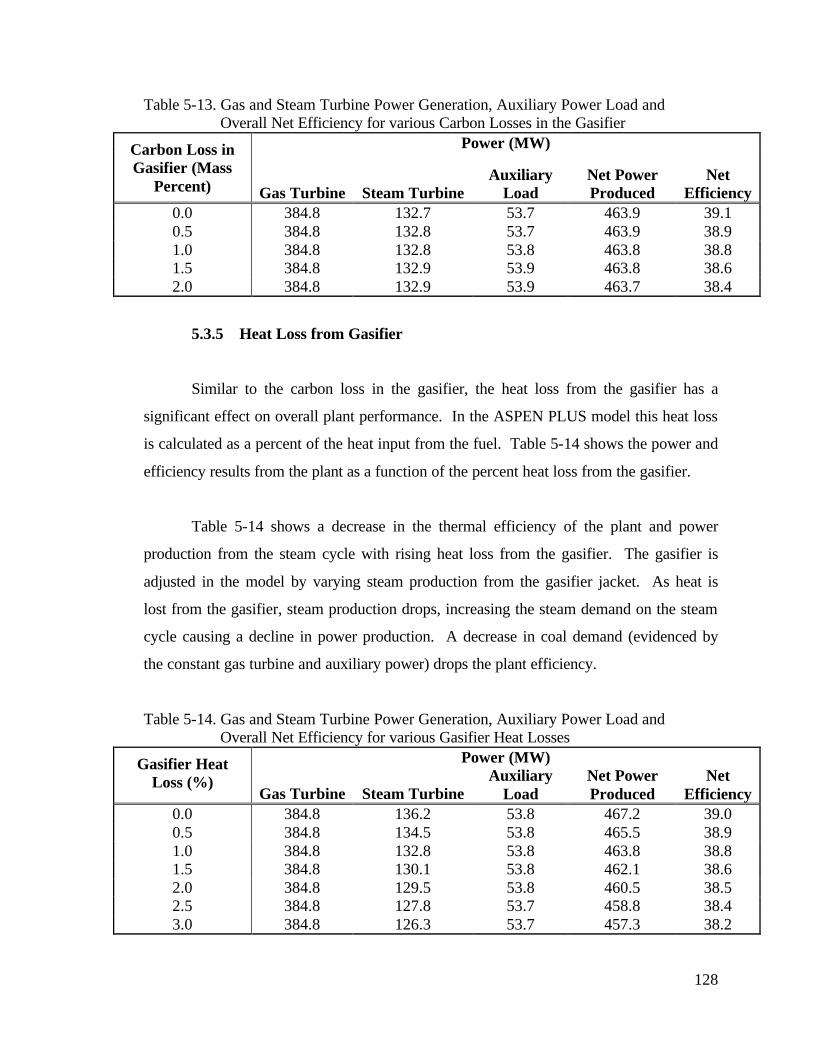
128

Table 5-13. Gas and Steam Turbine Power Generation, Auxiliary Power Load and Overall Net Efficiency for various Carbon Losses in the Gasifier

Power (MW) Carbon Loss in Gasifier (Mass

Percent) Gas Turbine Steam Turbine Auxiliary

Load Net Power Produced

Net Efficiency

0.0 384.8 132.7 53.7 463.9 39.1 0.5 384.8 132.8 53.7 463.9 38.9 1.0 384.8 132.8 53.8 463.8 38.8 1.5 384.8 132.9 53.9 463.8 38.6 2.0 384.8 132.9 53.9 463.7 38.4

5.3.5 Heat Loss from Gasifier

Similar to the carbon loss in the gasifier, the heat loss from the gasifier has a

significant effect on overall plant performance. In the ASPEN PLUS model this heat loss

is calculated as a percent of the heat input from the fuel. Table 5-14 shows the power and

efficiency results from the plant as a function of the percent heat loss from the gasifier.

Table 5-14 shows a decrease in the thermal efficiency of the plant and power

production from the steam cycle with rising heat loss from the gasifier. The gasifier is

adjusted in the model by varying steam production from the gasifier jacket. As heat is

lost from the gasifier, steam production drops, increasing the steam demand on the steam

cycle causing a decline in power production. A decrease in coal demand (evidenced by

the constant gas turbine and auxiliary power) drops the plant efficiency.

Table 5-14. Gas and Steam Turbine Power Generation, Auxiliary Power Load and Overall Net Efficiency for various Gasifier Heat Losses

Power (MW) Gasifier Heat Loss (%)

Gas Turbine Steam Turbine Auxiliary

Load Net Power Produced

Net Efficiency

0.0 384.8 136.2 53.8 467.2 39.0 0.5 384.8 134.5 53.8 465.5 38.9 1.0 384.8 132.8 53.8 463.8 38.8 1.5 384.8 130.1 53.8 462.1 38.6 2.0 384.8 129.5 53.8 460.5 38.5 2.5 384.8 127.8 53.7 458.8 38.4 3.0 384.8 126.3 53.7 457.3 38.2

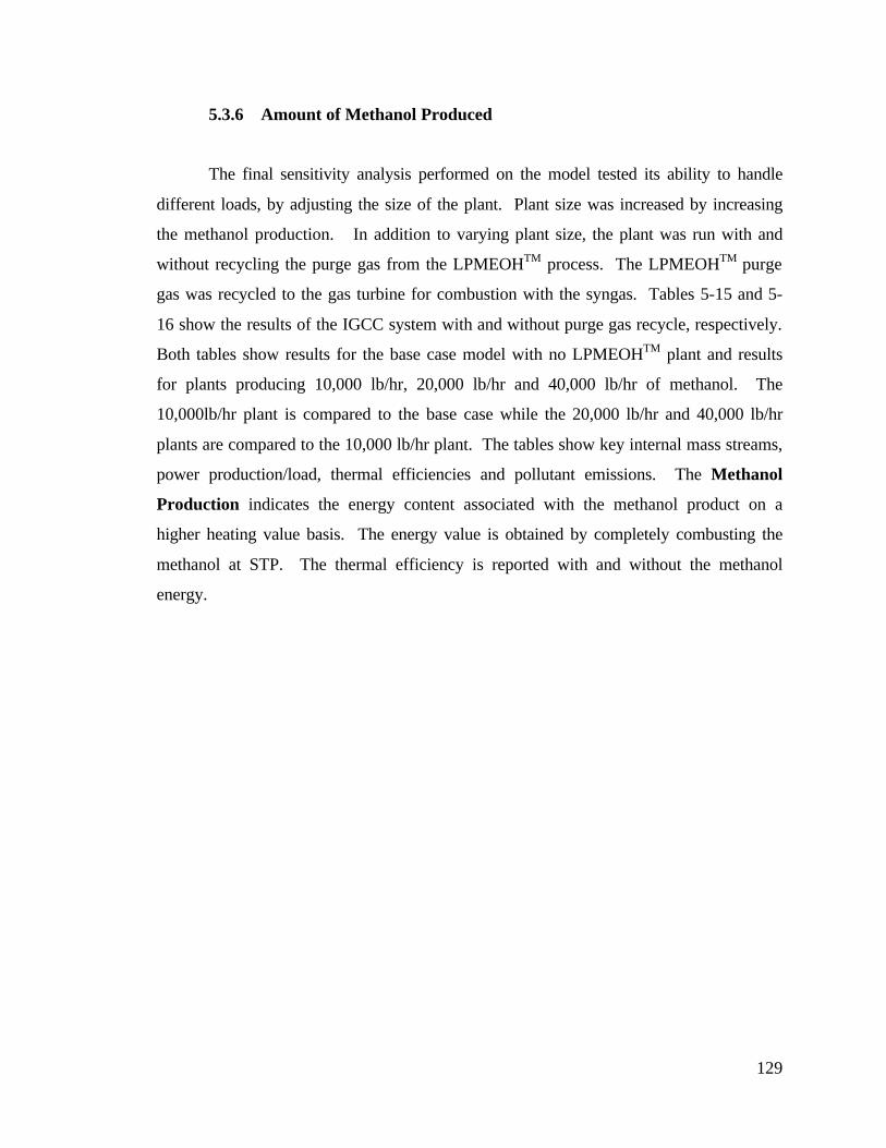
129

5.3.6 Amount of Methanol Produced

The final sensitivity analysis performed on the model tested its ability to handle

different loads, by adjusting the size of the plant. Plant size was increased by increasing

the methanol production. In addition to varying plant size, the plant was run with and

without recycling the purge gas from the LPMEOHTM process. The LPMEOHTM purge

gas was recycled to the gas turbine for combustion with the syngas. Tables 5-15 and 5-

16 show the results of the IGCC system with and without purge gas recycle, respectively.

Both tables show results for the base case model with no LPMEOHTM plant and results

for plants producing 10,000 lb/hr, 20,000 lb/hr and 40,000 lb/hr of methanol. The

10,000lb/hr plant is compared to the base case while the 20,000 lb/hr and 40,000 lb/hr

plants are compared to the 10,000 lb/hr plant. The tables show key internal mass streams,

power production/load, thermal efficiencies and pollutant emissions. The Methanol

Production indicates the energy content associated with the methanol product on a

higher heating value basis. The energy value is obtained by completely combusting the

methanol at STP. The thermal efficiency is reported with and without the methanol

energy.

130

Table 5-15. IGCC Plant Size Sensitivity Analysis Firing Pittsburgh No. 8 Coal with Purge Recycle

IGCC 10,000 lb/hr 20,000 lb/hr 40,000 lb/hr Massflow Massflow Difference Massflow Difference Massflow Difference

Mass Flow Rates lb/hr lb/hr From IGCC lb/hr From 10k lb/hr From 10k To Gasifier Fuel 314,540 326,982 4.0% 337,277 3.4% 357,844 9.4%

Oxygen 181,368 187,822 3.6% 193,556 3.1% 205,008 9.1% Steam 106,159 109,936 3.6% 113,293 3.1% 119,995 9.1%

Quench Water 513,176 531,464 3.6% 547,690 3.1% 580,116 9.2% Crude Syngas 648,671 671,793 3.6% 692,277 3.0% 733,184 9.1% Clean Syngas to Saturator 511,159 473,939 -7.3% 434,834 -8.3% 356,482 -24.8% Clean Syngas to Methanol 55,224 110,449 100.0% 220,992 300.2% Total Clean Syngas 511,159 531,181 3.9% 547,363 3.0% 579,677 9.1% Feed Syngas to Gas Turbine 943,723 957,835 1.5% 968,483 1.1% 989,678 3.3% Air to Gas Turbine 6,936,730 6,922,200 -0.2% 6,912,270 -0.1% 6,892,330 -0.4% Purge Gas from Methanol 44,862 89,732 100.0% 179,560 300.3% Total Feed to Saturator 513,176 518,800 1.1% 524,566 1.1% 536,042 3.3% Fuel Mixture in Gas Turbine 6,631,940 6,634,040 0.0% 6,636,550 0.0% 6,641,390 0.1% Methanol 10,001 19,999 100.0% 39,999 300.0% Overall Water Consumption 510,921 519,824 1.7% 526,842 1.3% 540,796 4.0% Production of Sulfur 9,916 10,296 3.8% 10,612 3.1% 11,241 9.2% Slag Production 46,113 47,937 4.0% 49,447 3.1% 52,462 9.4%

Steam to Methanol Process 7,966 15,931 100.0% 31,873 300.1% Saturation Water 394,417 399,512 1.3% 403,185 0.9% 410,485 2.7%

Steam for Saturation Heating 297,067 283,925 -4.4% 270,869 -4.6% 244,676 -13.8% MW MW MW MW

Gas Turbines 383.9 384.6 0.2% 385.1 0.1% 386.0 0.4% Steam Turbines 131.6 134.6 2.2% 134.8 0.2% 135.7 0.8% Gross Power 515.5 519.2 0.7% 519.9 0.1% 521.7 0.5% Auxiliary Loads 48.1 53.9 11.9% 59.4 10.3% 70.4 30.8% Power to Grid 467.4 465.4 -0.4% 460.5 -1.0% 451.3 -3.0% Methanol Production 11.4 22.9 100.0% 45.8 300.0% Total Power (w/Methanol) 476.8 483.4 1.4% 497.0 4.2% Power Thermal Efficiency

HHV BASIS 41.1% 39.3% -4.2% 37.7% -4.1% 34.8% -11.4% LHV BASIS 42.8% 41.0% -4.2% 39.3% -4.1% 36.3% -11.4%

Combined Thermal Efficiency HHV BASIS 40.3% 39.6% -1.7% 38.4% -4.7% LHV BASIS 42.0% 41.3% -1.7% 40.0% -4.7%

Pollutant Emissions

SO2 (lb/MMBTU) 4.38 x 10-4 4.82 x 10-4 9.8% 4.88 x 10-4 1.3% 5.00 x 10-4 3.9% CO2 (lb/kWh) 1.70 1.73 2.2% 1.78 2.5% 1.86 7.4% NOx (ppm, @ 15% O2, dry) 10.1 9.94 -1.9% 9.93 -0.1% 9.74 -2.0% CO (ppm, @ 15% O2, dry) 0.483 0.482 -0.1% 0.488 1.1% 0.491 1.7% PM (lb/hr) 23.6 23.6 0.0% 23.6 0.0% 23.6 0.0% HC (lb/hr) 20.5 20.5 0.0% 20.5 0.0% 20.5 0.0%

131

Table 5-16. IGCC Plant and Sensitivity Analysis Firing Pittsburgh No. 8 Coal with No Purge Gas Recycle

IGCC 10,000 lb/hr 20,000 lb/hr 40,000 lb/hr Massflow Massflow Difference Massflow Difference Massflow Difference

Mass Flow Rates lb/hr lb/hr From IGCC lb/hr From 10k lb/hr From 10k To Gasifier Fuel 314,540 352,151 12.0% 387,600 10.1% 458,566 30%

Oxygen 181,368 201,838 11.3% 221,584 9.8% 261,111 29% Steam 106,159 118,140 11.3% 129,698 9.8% 152,834 29%

Quench Water 513,176 571,095 11.3% 627,003 9.8% 738,948 29% Crude Syngas 648,671 721,884 11.3% 792,419 9.8% 933,648 29% Clean Syngas to Saturator 511,159 513,343 0.4% 513,552 0.0% 513,990 0.1% Clean Syngas to Methanol 55,241 110,538 100% 221,240 300% Total Clean Syngas 511,159 570,753 11.7% 626,470 9.8% 738,035 29% Feed Syngas to Gas Turbine 943,723 947,775 0.4% 948,180 0.0% 949,027 0.1% Air to Gas Turbine 6,936,730 6,931,560 -0.1% 6,930,780 0.0% 6,930,530 0.0% Purge Gas from Methanol 44,864 89,794 100% 179,792 301% Total Feed to Saturator 513,176 513,343 0.0% 513,552 0.0% 513,990 0.1% Fuel Mixture in Gas Turbine 6,631,940 6,631,650 0.0% 6,631,420 0.0% 6,632,060 0.0% Methanol 9,999 19,999 100% 40,000 300% Overall Water Consumption 510,921 520,414 1.9% 527,919 1.4% 542,961 4.3% Production of Sulfur 9,916 11,067 11.6% 12,152 9.8% 14,325 29% Slag Production 46,113 51,627 12.0% 56,824 10.1% 67,228 30%

Steam to Methanol Process 7,967 15,939 100% 31,894 300% Saturation Water 394,417 391,956 -0.6% 387,981 -1.0% 380,040 -3.0%

Steam for Saturation Heating 297,067 271,789 -8.5% 246,515 -9% 195,782 -28% MW MW MW MW

Gas Turbines 383.9 384.2 0.1% 384.2 0.0% 384.3 0.0% Steam Turbines 131.6 134.4 2.1% 134.9 0.3% 135.9 1.1% Gross Power 515.5 518.6 0.6% 519.1 0.1% 520.2 0.3% Auxiliary Loads 48.1 54.3 13% 60.2 10.9% 72.1 33% Power to Grid 467.4 464.4 -0.6% 458.9 -1.2% 448.1 -3.5% Methanol Production 11.4 22.9 100% 45.8 300% Total Power (w/Methanol) 475.8 481.8 1.3% 493.9 3.8% Power Thermal Efficiency

HHV BASIS 41.1% 36.4% -11.3% 32.7% -10.2% 27.0% -25.9% LHV BASIS 42.8% 38.0% -11.3% 34.1% -10.2% 28.1% -25.9%

Combined Thermal Efficiency HHV BASIS 37.3% 34.3% -8.0% 29.8% -20.3% LHV BASIS 38.9% 35.8% -8.0% 31.0% -20.3%

Pollutant Emissions

SO2 (lb/MMBTU) 4.38 x 10-4 4.43 x 10-4 1.0% 4.44 x 10-4 0.3% 4.47 x 10-4 0.8% CO2 (lb/kWh) 1.70 1.71 1.1% 1.74 1.3% 1.78 4.0% NOx (ppm, @ 15% O2, dry) 10.1 10.1 0.0% 10.1 0.1% 10.1 0.0% CO (ppm, @ 15% O2, dry) 0.483 0.486 0.5% 0.486 0.1% 0.486 0.1% PM (lb/hr) 23.6 23.6 0.0% 23.6 0.0% 23.6 0.0% HC (lb/hr) 20.5 20.5 0.0% 20.5 0.0% 20.5 0.0%

The most significant difference, applicable in both tables, is that the Fuel feed to

the Gasifier increases at a rate greater than the other inputs to the gasifier. The other

132

three inputs to the gasifier, i.e. Oxidant, Steam and Quench Water, all rise at the same

rate for a given plant size. A comparison of the two tables implies that as the need for

more fuel increases, the amount of Oxidant, Steam and Quench Water increases at a

lesser rate.

Table 5-15 shows that growth in the methanol plant size lowers the overall

efficiency of the plant and that power generation decreases. When comparing the

efficiency of the plants on a strict power basis, the thermal efficiency decreases by 11.4

percent between the base case and the 40,000 lb/hr case. However, when accounting for

the energy value of the methanol, the thermal efficiency decreases by only 4.7 percent.

The same scenario in the study where the methanol purge gas was not recycled to the gas

turbine provides a more significant difference. When comparing the efficiency of the

non-purge-recycling plants (Table 5-16) on a strict power basis the thermal efficiency

decreases by 25.9 percent between the base case and the 40,000 lb/hr case. When taking

into account the energy associated with the methanol product the thermal efficiency drops

by 20.3 percent. Differences in thermal efficiency with and without methanol show the

significance of the purge gas to the IGCC system.

Table 5-15 shows a significant increase of 2.1 MW in the power production from

the gas turbine, indicating a change in the syngas composition for the purge gas recycle

scenario. Table 5-17 confirms a changing fuel gas molar composition for each methanol

plant size with purge gas recycle. As the size of the methanol plant increases, the amount

of purge gas from the methanol plant increases while the amount of clean syngas fed to

the gas turbine remains approximately constant. This changes the composition and

heating value of the fuel gas, thus changing the amount of power produced from the gas

turbine.

133

Table 5-17. Fired Syngas Composition Variance with Plant Size with Purge Gas Recycle Amount of Methanol Produced (lb/hr) Component 0 10000 20000 40000

H2 15.3% 14.4% 13.5% 11.7% H2O 48.0% 48.5% 48.9% 49.8% CH4 4.2% 4.3% 4.5% 4.7% CO 30.4% 30.7% 31.0% 31.6% Other 1.9% 2.0% 2.0% 2.0% CH4O 0.0% 3.5E-04% 7.0E-04% 1.0E-03%

134

6.0 APPLICATION OF THE PERFORMANCE AND EMISSIONS MODEL OF THE BGL SLAGGING GASIFIER-BASED IGCC SYSTEM WITH METHANOL PRODUCTION FIRING MULTIPLE FUELS

This chapter presents results of the model firing different fuels in case studies.

For calibration and verification purposes, the model has only been firing Pittsburgh No. 8

bituminous coal. However, the motivation of this study was to simulate MSW

gasification rather than coal gasification. Previous data was available only for a coal-

firing IGCC system making it necessary to first develop the coal-fired model then fuel it

with other feedstocks.

6.1 Fuels

Three fuels are used in this study: a Pittsburgh No. 8 bituminous coal; a German

waste blend; and an American 75/25 percent mixture of RDF and Pittsburgh No. 8

Bituminous coal. The Pittsburgh No. 8 coal is included because it was used to develop

the model. The German waste blend consists of 13 percent plastics, 22 percent sewage

sludge, 13 percent automobile industry waste, 39 percent RDF, and 13 percent Polish

bituminous coal (Vierrath, 1999). The proximate and ultimate for each of these wastes

are shown in Table 6-1. Using a weighted average with the values of Table 6-1 and the

aforementioned blend, the composition of the German waste fuel was calculated. The

BGL gasifier firing waste was calibrated with the “German Blend” and a corresponding

crude syngas provided by Lurgi. This was the only data available at the time of this study

from the newly installed BGL gasifiers firing waste at the Pumpe Schwarze plant in

Dresden, Germany.

Dr. Helmut Vierrath of Lurgi Umwelt GmbH FRG, indicated in a personal

interview that Lurgi had the most success at the Schwarze Pumpe plant firing a mix of 75

percent RDF and 25 percent Polish Bituminous coal (Vierrath, 1999). However, the RDF

used in the Schwarze Pumpe plant was significantly different than a “typical” RDF from

the United States. A third fuel, consisting of the recommended 75 percent RDF and 25

135

percent bituminous coal, using a typical American RDF and Pittsburgh No. 8 bituminous

coal was fired in the model (Tchobanoglous et. al, 1993 and Gupta and Rohrbach, 1991).

Table 6-2 provides the proximate and ultimate analyses of the Pittsburgh No. 8 Coal,

American waste and German waste fuels. Tables 6-1 and 6-2 report the fuel composition

as entered in the ASPEN PLUS model, i.e., the fixed carbon, volatile matter and ash of

the proximate analysis are on a dry basis.

Table 6-1. Proximate and Ultimate Analysis of German Wastes and American RDF

Proximate Analysis Sewage Auto Plastics German Polish American (dry wt%) Sludge Waste RDF Coal RDF

Moisture (wt%) 2.7 5.0 10.8 4.2 5.7 10.5 Fixed Carbon 7.5 12.1 8.1 9.0 51.5 15.0 Volatile Matter 79.4 57.6 51.0 75.5 39.8 75.0 Ash 13.1 30.3 40.9 15.5 8.7 10.0 Ultimate Analysis

(dry wt%) Carbon 63.15 44.74 32.07 48.28 74.40 44.7 Hydrogen 8.69 5.99 4.75 6.89 4.75 6.2 Nitrogen 3.22 2.02 8.10 0.84 1.36 0.7 Sulfur 1.54 2.99 1.67 1.04 0.45 0.0 Oxygen 10.35 13.94 12.49 27.40 10.34 38.4 Ash 13.05 30.31 40.92 15.55 8.70 10.0 HHV – (BTU/lb) 13,494 8,875 5,601 8,713 13,317 8,868

Table 6-2. Proximate and Ultimate Analysis of Pittsburgh No. 8 Coal, American Waste Fuel and German Waste Fuel

Proximate Analysis, dry wt% Pittsburgh No. 8 American German Moisture (wt%) 6.00 9.6 5.1 Fixed Carbon 48.94 17.5 15.9 Volatile Matter 38.83 72.0 65.0 Ash 12.23 10.5 19.1

Ultimate Analysis, dry wt% Carbon 73.21 52.1 52.6 Hydrogen 4.94 5.9 6.6 Nitrogen 1.38 0.9 2.5 Sulfur 3.39 0.9 1.4 Oxygen 4.85 29.7 17.8 Ash 12.23 10.3 19.1

HHV – Dry Basis (BTU/lb) 13,138 9,999 10,026

136

The German waste is processed at a RDF pellet production plant in Berlin from

household waste, shredder light fraction, plastics and contaminated wood (Vierrath et al.,

1997). After removing iron and other metals and drying, the “fluff” is pelletized on an

annular pelletizing press using a binder, such as bituminous coal, to achieve the necessary

strength both for transportation to the plant and thermal stability in the gasifier (Vierrath

et al., 1997). The American RDF is classified as RDF-5 or densified RDF (d-RDF)

(Gupta and Rohrbach, 1991). RDF-5 is first processed by removing the metals, glass and

other entrained organics before reshredding so that 95 weight percent passes through a

two-inch square mesh screen. The combustible fraction of the waste is then densified

into pellets, briquettes, or some similar form (Gupta and Rohrbach, 1991). As suggested

in Tchobanoglous (1993), ASPEN PLUS calculates the heating value for the American

RDF using the Dulong correlation, which is provided in Appendix B.

6.2 Calibration of Model Firing German MSW/Coal Mixture

The large difference in compositions of coal and waste requires model

recalibration when firing waste derived fuel. Lurgi Umwelt GmbH FRG provided

preliminary results from firing a waste derived fuel in the BGL Slagging gasifier at the

IGCC plant in Dresden, Germany. Section 6.1 gives a description of the fuel, including

the proximate and ultimate analysis, provided by Lurgi. A corresponding crude syngas

composition, also provided by Lurgi, was used to calibrate the gasification island for

firing waste fuels. The model was calibrated by adjusting the reaction temperatures in

the GASIFXR unit operation block. Table 6-3 lists all the input assumptions used in

model calibration. Table 6-4 compares the crude syngas from the calibrated model to the

crude syngas from Lurgi. The results are shown on a dry, mole percent basis.

137

Table 6-3. Input Assumptions for Calibration of the Gasification Island to Waste Fuel

Coal Feed Rate 31.555 tons/hr Nitrogen for Pressurization 1,653 lb/hr Combustion Zone Temperature 3,196 °F Gasification Zone Temperature 1,300 °F Heat Loss from Gasifier 1.0 % Exiting Syngas Temperature 284 °F Fraction of Carbon in Slag 1 % Fraction of Sulfur in Slag 3 % Steam-to-oxygen Molar Ratio 1.087 Approach Temperatures in GASIFXR Block Equations (3-11) to (3-14), Respectively +520 °F; +440 °F; +200 °F; -200 °F

Table 6-4. Comparison of Lurgi and ASPEN PLUS Crude Syngas Composition Component ASPENPLUS Lurgi Percent (dry basis) Model (mole%) Data (mole%) Error

CO2 4.56 7.28 -37.42 CO 46.26 46.26 0.00 H2 36.80 36.35 1.24 CH4 8.06 5.92 36.16 CnHm 0.66 0.52 27.70 H2S 0.58 0.47 24.28 N2 2.92 3.20 -8.73

Table 6-4 shows the calibration of the ASPEN PLUS model to the Lurgi BGL

gasifier to differ by more than 20 percent in four of the seven components. However, the

four components make up only 14.19 mole-percent of the crude syngas. The two most

significant components of the syngas, H2 and CO, differ by only 1.24 percent and

constitute over 80 mole-percent of the crude syngas. The non-methane hydrocarbons

(CnHm) differ by 27.70 percent from the Lurgi case because of assumptions made for

model simplification. In ASPEN PLUS non-methane hydrocarbons were simulated using

only generic formulas such as tars, phenols, naphtha and oils (refer to Section 3.2.1).

The assumption that all sulfur is converted into H2S results in the difference in the

H2S component between the model and Lurgi. Actually, the Lurgi data has COS, CS2,

H2S and “other” components included in the H2S component.

138

Table 6-4 shows that the model over-estimates CH4 by 36.16 percent and under-

estimates CO2 by 37.42 percent. This inconsistency implies that the carbon being used to

produce CH4 should be in CO2 production. However, the ASPEN PLUS model does not

have a method to simultaneously decrease the CH4 composition and increase the CO2

composition without significantly affecting the CO and H2 compositions because of the

equations used in the GASFIXR unit operation block. Since CO and H2 are more

significant in the operation of the IGCC system and therefore more of a concern model

calibration, no steps were taken to alter the results of the calibration given in Table 6-4.

6.3 Model Application

Three example case studies are presented here to illustrate the new IGCC system

model. Each case study involves three plant sizes, which either recycle of vent the purge

gas from the LPMEOHTM plant, for a total of six scenarios per case study. Each case

study will differ by the type of fuel fed; Pittsburgh No. 8 coal, German waste blend or

American RDF/coal blend.

6.3.1 Input Assumptions

Model input assumptions for the performance and emission model were

developed based on a review of design and performance parameters obtained from the

literature (Eustis and Paffenbarger, 1990; Farmer, 1997; Frey and Rubin, 1990; Pechtl et

al., 1992; STONE, 1991; Vaswani, 2000; Vierrath, 1999). Configuration of the model

represents two parallel trains of heavy-duty “Frame 7F” gas turbines.

Focusing on parameters in the gasification island, Table 6-5 summarizes many of

the key input assumptions made for each fuel fired. Many of these assumptions are

previously described in the technical description of the model. Since there are hundreds

of input assumptions in the model, Table 6-5 lists only the most significant parameters

affecting plant design and performance.

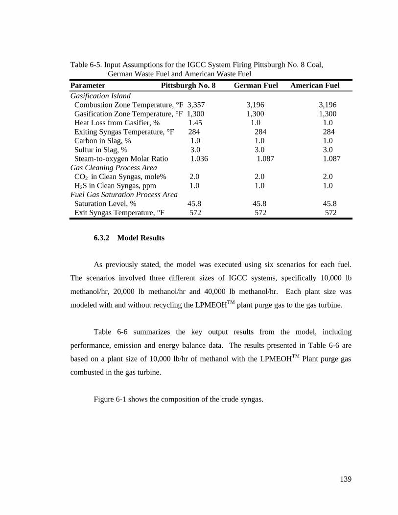
139

Table 6-5. Input Assumptions for the IGCC System Firing Pittsburgh No. 8 Coal, German Waste Fuel and American Waste Fuel

Parameter Pittsburgh No. 8 German Fuel American Fuel Gasification Island Combustion Zone Temperature, °F 3,357 3,196 3,196 Gasification Zone Temperature, °F 1,300 1,300 1,300 Heat Loss from Gasifier, % 1.45 1.0 1.0 Exiting Syngas Temperature, °F 284 284 284 Carbon in Slag, % 1.0 1.0 1.0 Sulfur in Slag, % 3.0 3.0 3.0 Steam-to-oxygen Molar Ratio 1.036 1.087 1.087 Gas Cleaning Process Area CO2 in Clean Syngas, mole% 2.0 2.0 2.0 H2S in Clean Syngas, ppm 1.0 1.0 1.0 Fuel Gas Saturation Process Area Saturation Level, % 45.8 45.8 45.8 Exit Syngas Temperature, °F 572 572 572

6.3.2 Model Results

As previously stated, the model was executed using six scenarios for each fuel.

The scenarios involved three different sizes of IGCC systems, specifically 10,000 lb

methanol/hr, 20,000 lb methanol/hr and 40,000 lb methanol/hr. Each plant size was

modeled with and without recycling the LPMEOHTM plant purge gas to the gas turbine.

Table 6-6 summarizes the key output results from the model, including

performance, emission and energy balance data. The results presented in Table 6-6 are

based on a plant size of 10,000 lb/hr of methanol with the LPMEOHTM Plant purge gas

combusted in the gas turbine.

Figure 6-1 shows the composition of the crude syngas.

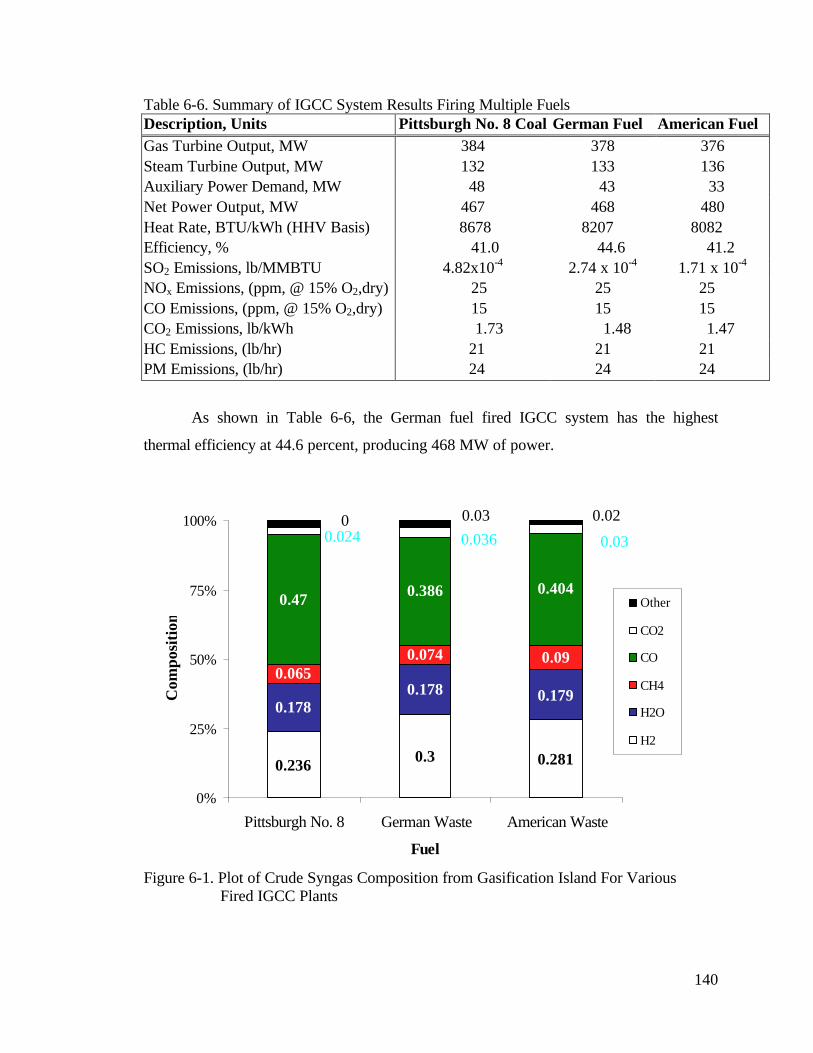
140

Table 6-6. Summary of IGCC System Results Firing Multiple Fuels Description, Units Pittsburgh No. 8 Coal German Fuel American Fuel Gas Turbine Output, MW 384 378 376 Steam Turbine Output, MW 132 133 136 Auxiliary Power Demand, MW 48 43 33 Net Power Output, MW 467 468 480 Heat Rate, BTU/kWh (HHV Basis) 8678 8207 8082 Efficiency, % 41.0 44.6 41.2 SO2 Emissions, lb/MMBTU 4.82x10-4 2.74 x 10-4 1.71 x 10-4 NOx Emissions, (ppm, @ 15% O2,dry) 25 25 25 CO Emissions, (ppm, @ 15% O2,dry) 15 15 15 CO2 Emissions, lb/kWh 1.73 1.48 1.47 HC Emissions, (lb/hr) 21 21 21 PM Emissions, (lb/hr) 24 24 24

As shown in Table 6-6, the German fuel fired IGCC system has the highest

thermal efficiency at 44.6 percent, producing 468 MW of power.

Figure 6-1. Plot of Crude Syngas Composition from Gasification Island For Various Fired IGCC Plants

0.236 0.3 0.281

0.1780.178 0.179

0.0650.074 0.09

0.47 0.386 0.404

0.030.0360.0240.020.03 0

0%

25%

50%

75%

100%

Pittsburgh No. 8 German Waste American Waste

Fuel

Com

posi

tion

Other

CO2

CO

CH4

H2O

H2

141

The crude syngas composition varies significantly between the three different

fuels, as shown in Figure 6-1. The black column marked “Other” includes the N2, H2S,

Naphtha and Oil compounds. While the H2O composition remains fairly constant at 17.8

percent, the CO composition varies from 38.6 to 47.0 mole percent, CH4 ranges from 6.5

to 9.0 mole percent and H2 varies from 23.6 to 30.0 mole percent over the spectrum of

fuels.

Tables 6-7 and 6-8 summarize the results for the various sized IGCC systems

firing German RDF with and without purge gas recycling, respectively. Tables 6-9 and

6-10 summarize the results for the various sized IGCC systems firing American RDF

with and without purge gas recycling, respectively. The results from multiple plant sizes

firing Pittsburgh No. 8 Coal are shown in Table 5-15 and Table 5-16.

Regardless of the type of fuel fired in the IGCC system, the overall thermal

efficiency drops as the methanol plant size increases. With either fuel, the overall

thermal efficiency is greater when the LPMEOHTM Plant purge gas is recycled to the gas

turbine. From Tables 6-9 and 6-10, an American coal and RDF blend fired IGCC system

with a 10,000 lb methanol/hr plant, has an overall thermal efficiency of 42.2 percent

(HHV basis) with purge gas recycling and 39.6 percent without. The IGCC systems

firing the German waste blend report similar findings of 45.7 percent overall thermal

efficiency with purge gas recycling and 43.0 percent without purge gas recycling for a

10,000 lb methanol/hr sized plant. There is not a significant difference in the overall

thermal efficiencies between the fuels for the purge gas recycle scenario. However, the

German RDF fired plants are roughly one percent less efficient with out purge gas

recycling than with purge gas recycling.

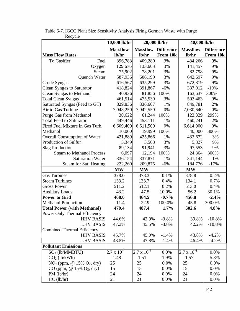
142

Table 6-7. IGCC Plant Size Sensitivity Analysis Firing German Waste with Purge Recycle

10,000 lb/hr 20,000 lb/hr 40,000 lb/hr

Massflow Massflow Difference Massflow Difference Mass Flow Rates lb/hr lb/hr From 10k lb/hr From 10k

To Gasifier Fuel 396,783 409,280 3% 434,266 9% Oxygen 129,676 133,603 3% 141,457 9%

Steam 75,902 78,201 3% 82,798 9% Quench Water 587,936 606,199 3% 642,697 9%

Crude Syngas 616,567 635,299 3% 672,819 9% Clean Syngas to Saturator 418,824 391,867 -6% 337,912 -19% Clean Syngas to Methanol 40,936 81,856 100% 163,637 300% Total Clean Syngas 461,514 475,530 3% 503,463 9% Saturated Syngas (Feed to GT) 829,836 836,607 1% 849,781 2% Air to Gas Turbine 7,048,250 7,042,550 0% 7,030,640 0% Purge Gas from Methanol 30,622 61,244 100% 122,329 299% Total Feed to Saturator 449,446 453,111 1% 460,241 2% Fired Fuel Mixture in Gas Turb. 6,609,400 6,611,500 0% 6,614,900 0% Methanol 10,000 19,999 100% 40,000 300% Overall Consumption of Water 421,889 425,866 1% 433,672 3% Production of Sulfur 5,349 5,508 3% 5,827 9% Slag Production 89,134 91,941 3% 97,553 9%

Steam to Methanol Process 6,097 12,194 100% 24,364 300% Saturation Water 336,154 337,871 1% 341,144 1%

Steam for Sat. Heating 222,260 209,875 -6% 184,776 -17% MW MW MW

Gas Turbines 378.0 378.3 0.1% 378.8 0.2% Steam Turbines 133.2 133.7 0.4% 134.1 0.7% Gross Power 511.2 512.1 0.2% 513.0 0.4% Auxiliary Loads 43.2 47.5 10.0% 56.2 30.1% Power to Grid 468.0 464.5 -0.7% 456.8 -2.4% Methanol Production 11.4 22.9 100.0% 45.8 300.0% Total Power (with Methanol) 479.4 487.4 1.7% 502.6 4.8% Power Only Thermal Efficiency

HHV BASIS 44.6% 42.9% -3.8% 39.8% -10.8% LHV BASIS 47.3% 45.5% -3.8% 42.2% -10.8%

Combined Thermal Efficiency HHV BASIS 45.7% 45.0% -1.4% 43.8% -4.2% LHV BASIS 48.5% 47.8% -1.4% 46.4% -4.2%

Pollutant Emissions SO2 (lb/MMBTU) 2.7 x 10-4 2.7 x 10-4 0.0% 2.7 x 10-4 0.0% CO2 (lb/kWh) 1.48 1.51 1.9% 1.57 5.8% NOx (ppm, @ 15% O2, dry) 25 25 0.0% 25 0.0% CO (ppm, @ 15% O2, dry) 15 15 0.0% 15 0.0% PM (lb/hr) 24 24 0.0% 24 0.0% HC (lb/hr) 21 21 0.0% 21 0.0%

143

Table 6-8. IGCC Plant Size Sensitivity Analysis Firing German RDF with No Purge Recycling

10,000 lb/hr 20,000 lb/hr 40,000 lb/hr Massflow Massflow Difference Massflow Difference Mass Flow Rates lb/hr lb/hr From 10k lb/hr From 10k To Gasifier Fuel 421,985 457,622 8% 528,937 25%

Oxygen 136,762 148,285 8% 171,339 25% Steam 80,050 86,794 8% 100,289 25%

Quench Water 577,428 626,025 8% 723,224 25% Crude Syngas 656,659 711,920 8% 822,503 25% Clean Syngas to Saturator 445,383 445,220 0% 444,989 0% Clean Syngas to Methanol 41,106 82,193 100% 164,331 300% Total Clean Syngas 488,345 529,425 8% 611,644 25% Saturated Syngas (Feed to GT) 822,346 822,064 0% 821,672 0% Air to Gas Turbine 7,056,330 7,056,330 0% 7,056,330 0% Purge Gas from Methanol 30,788 61,571 100% 123,047 300% Total Feed to Saturator 445,383 445,220 0% 444,989 0% Fired Fuel Mixture in Gas Turbine 6,608,540 6,608,260 0% 6,607,870 0% Methanol 10,000 19,999 100% 39,998 300% Overall Consumption of Water 419,424 422,211 1% 427,750 2% Production of Sulfur 5,674 6,129 8% 7,039 24% Slag Production 94,795 102,801 8% 118,821 25% Steam to Methanol Process 6,120 12,239 100% 24,470 300% Saturation Water 330,510 326,485 -1% 318,517 -4% Steam for Sat. Heating 202,623 179,823 -11% 134,270 -34% MW MW MW Gas Turbines 377.6 377.6 0.0% 377.5 0.0% Steam Turbines 133.9 134.2 0.2% 134.3 0.3% Gross Power 511.5 511.8 0.0% 511.8 0.1% Auxiliary Loads 42.9 47.0 9.7% 55.3 29.0% Power to Grid 468.6 464.7 -0.8% 456.4 -2.6% Methanol Production 11.4 22.9 100.0% 45.8 300.0% Total Power (with Methanol) 480.1 487.6 1.6% 502.2 4.6% Power Only Thermal Efficiency HHV BASIS 42.0% 38.4% -8.6% 32.6% -22.3% LHV BASIS 44.6% 40.8% -8.6% 34.6% -22.3% Combined Thermal Efficiency HHV BASIS 43.0% 40.3% -6.3% 35.9% -16.5% LHV BASIS 45.7% 42.8% -6.3% 38.1% -16.5% Pollutant Emissions SO2 (lb/MMBTU) 2.6 x 10-4 2.6 x 10-4 0.0% 2.6 x 10-4 0.0% CO2 (lb/kWh) 1.46 1.48 0.9% 1.50 2.8% NOx (ppm, @ 15% O2, dry) 25 25 0.0% 25 0.0% CO (ppm, @ 15% O2, dry) 15 15 0.0% 15 0.0% PM (lb/hr) 24 24 0.0% 24 0.0% HC (lb/hr) 21 21 0.0% 21 0.0%

144

Table 6-9. IGCC Plant Size Sensitivity Analysis Firing American RDF with Purge Recycle

10,000 lb/hr 20,000 lb/hr 40,000 lb/hr Massflow Massflow Difference Massflow Difference Mass Flow Rates lb/hr lb/hr From 10k lb/hr From 10k To Gasifier Fuel 447,492 461,497 3% 489,534 9%

Oxygen 67,484 69,434 3% 73,371 9% Steam 39,482 40,622 3% 42,926 9%

Quench Water 466,626 480,765 3% 509,150 9% Crude Syngas 591,681 609,585 3% 645,535 9% Clean Syngas to Saturator 406,678 375,539 -8% 313,370 -23% Clean Syngas to Methanol 44,782 89,566 100% 179,135 300% Total Clean Syngas 453,182 466,880 3% 494,384 9% Saturated Syngas (Feed to GT) 814,410 820,488 1% 833,009 2% Air to Gas Turbine 7,072,700 7,067,470 0% 7,056,940 0% Purge Gas from Methanol 34,443 68,873 100% 137,820 300% Total Feed to Saturator 441,122 444,412 1% 451,190 2% Fired Fuel Mixture in Gas Turb. 6,614,030 6,615,820 0% 6,619,700 0% Methanol 10,000 20,000 100% 40,000 300% Overall Consumption of Water 391,411 394,357 1% 400,438 2% Production of Sulfur 3,796 3,906 3% 4,125 9% Slag Production 52,540 54,184 3% 57,476 9% Steam to Methanol Process 6,929 13,858 100% 27,718 300% Saturation Water 342,079 343,921 1% 347,762 2% Steam for Sat. Heating 225,295 211,917 -6% 185,486 -18% MW MW MW Gas Turbines 376.0 376.2 0.1% 376.7 0.2% Steam Turbines 136.1 136.9 0.6% 138.5 1.8% Gross Power 512.1 513.1 0.2% 515.2 0.6% Auxiliary Loads 32.6 36.8 13.1% 45.4 39.4% Power to Grid 479.5 476.3 -0.7% 469.8 -2.0% Methanol Production 11.4 22.9 100.0% 45.8 300.0% Total Power (with Methanol) 491.0 499.2 1.7% 515.5 5.0% Power Only Thermal Efficiency HHV BASIS 41.2% 39.7% -3.7% 36.9% -10.4% LHV BASIS 46.1% 44.4% -3.7% 41.3% -10.4% Combined Thermal Efficiency HHV BASIS 42.2% 41.6% -1.4% 40.5% -4.0% LHV BASIS 47.2% 46.5% -1.4% 45.3% -4.0% Pollutant Emissions SO2 (lb/MMBTU) 1.7 x 10-4 1.7 x 10-4 1.2% 1.8 x 10-4 3.4% CO2 (lb/kWh) 1.47 1.49 1.8% 1.55 5.5% NOx (ppm, @ 15% O2, dry) 25 25 0.0% 25 0.0% CO (ppm, @ 15% O2, dry) 15 15 0.0% 15 0.0% PM (lb/hr) 24 24 0.0% 24 0.0% HC (lb/hr) 21 21 0.0% 21 0.0%

145

Table 6-10. IGCC Plant Size Sensitivity Analysis Firing American RDF with No Purge Recycling

10,000 lb/hr 20,000 lb/hr 40,000 lb/hr Massflow Massflow Difference Massflow Difference Mass Flow Rates lb/hr lb/hr From 10k lb/hr From 10k To Gasifier Fuel 479,941 524,622 9% 614,007 28%

Oxygen 71,676 78,327 9% 91,626 28% Steam 41,934 45,825 9% 53,606 28%

Quench Water 460,175 503,009 9% 588,704 28% Crude Syngas 635,942 694,900 9% 812,834 28% Clean Syngas to Saturator 437,195 437,036 0% 436,822 0% Clean Syngas to Methanol 44,854 89,679 100% 179,240 300% Total Clean Syngas 483,888 528,725 9% 618,412 28% Saturated Syngas (Feed to GT) 807,171 806,893 0% 806,525 0% Air to Gas Turbine 7,079,900 7,079,900 0% 7,079,900 0% Purge Gas from Methanol 34,506 68,984 100% 137,912 300% Total Feed to Saturator 437,195 437,036 0% 436,822 0% Fired Fuel Mixture in Gas Turbine 6,612,690 6,612,410 0% 6,612,050 0% Methanol 9,999 20,000 100% 40,001 300% Overall Consumption of Water 387,977 389,511 0% 392,577 1% Production of Sulfur 4,053 4,403 9% 5,104 26% Slag Production 56,350 61,596 9% 72,091 28% Steam to Methanol Process 6,936 13,869 100% 27,723 300% Saturation Water 336,676 333,454 -1% 327,097 -3% Steam for Sat. Heating 205,543 181,538 -12% 133,946 -35%

MW MW MW Gas Turbines 375.7 375.6 0.0% 375.6 0.0% Steam Turbines 138.2 138.7 0.3% 139.6 1.0% Gross Power 513.9 514.3 0.1% 515.2 0.3% Auxiliary Loads 31.7 35.2 11.0% 42.2 33.0% Power to Grid 482.2 479.1 -0.6% 473.0 -1.9% Methanol Production 11.4 22.9 100.0% 45.8 300.0% Total Power (with Methanol) 493.6 502.0 1.7% 518.8 5.1% Power Only Thermal Efficiency HHV BASIS 38.7% 35.1% -9.1% 29.6% -23.3% LHV BASIS 43.2% 39.3% -9.1% 33.1% -23.3% Combined Thermal Efficiency HHV BASIS 39.6% 36.8% -7.0% 32.5% -17.9% LHV BASIS 44.2% 41.1% -7.0% 36.3% -17.9% Pollutant Emissions SO2 (lb/MMBTU) 1.6 x 10-4 1.6 x 10-4 0.0% 1.6 x 10-4 0.0% CO2 (lb/kWh) 1.44 1.45 0.7% 1.47 2.1% NOx (ppm, @ 15% O2, dry) 25 25 0.0% 25 0.0% CO (ppm, @ 15% O2, dry) 15 15 0.0% 15 0.0% PM (lb/hr) 24 24 0.0% 24 0.0% HC (lb/hr) 21 21 0.0% 21 0.0%

146

7.0 CONCLUSIONS AND RECOMMENDATIONS

This study developed a performance and emission model in ASPEN PLUS of a

BGL Slagging gasifer IGCC system with methanol co-production firing three different

fuels: (1) Pittsburgh No. 8 bituminous coal; (2) German waste fuel and (3) American

waste fuel.

The model is primarily based on findings of a study based by EPRI (Pechtl et al.,

1992). The EPRI study provided extensive process designs that were modified to fit the

scope of this study. To better simulate the BGL Slagging gasifier at the Schwarze Pumpe

plant, the gasification island was modified according to suggestions from Lurgi. The gas

turbine model was calibrated to both the latest published data for natural gas and to data

for firing syngas. The steam cycle was modified and calibrated to include four pressure

levels of steam generation. Auxiliary power models were developed for fuel preparation

and briquetting, fuel receiving and storage, the gasification island, Gas Liquor and

Separation, fuel gas saturation, BFW Treatment, the Power Island and the LPMEOHTM

Plant. The methanol production and operation of two gas turbines in series determine the

model size. Plant sizes of 10,000, 20,000 and 40,000 lb methanol/hr, each with and

without recycling the LPMEOHTM plant purge gas to the gas turbine, were modeled for

each fuel.

The following conclusions can be drawn from this study:

1. The gasification island variable that affected the model the most is the

combustion zone temperature. The net power produced from the plant

varied by 3.8 MW and the efficiency fluctuated 1.6 percent over the range of

combustion zone temperatures analyzed.

2. The steam cycle is most sensitive to changes in the intermediate-pressure

steam level.

147

3. The parameters that most affect the overall plant performance are: the

saturation level of the clean syngas; and the heat loss in the gasifier. The

saturation level of the syngas was varied from 0.35 mole-percent to 0.55

mole-percent affecting the net output of power in the plant by 11.6 MW.

The heat loss of the gasifier was varied from 0.0 to 3.0 percent and the

overall plant thermal efficiency was affected by 0.8 percent.

4. For a given fuel, recycling of the LPMEOHTM plant purge gas to the gas

turbine produced higher thermal efficiencies than venting the purge gas

because the energy from the purge gas is being recovered in the IGCC

system.

5. Larger plant sizes performed less efficiently than smaller plant sizes. The

10,000 lb methanol/hr plants ranged from 39.3 to 44.6 percent overall

thermal efficiency (HHV basis) while the 40,000 lb methanol/hr plants

ranged significantly less from 27.0 to 39.6 percent. The more methanol that

is produced, the closer the efficiency of the plant approaches the efficiency

of LPMEOHTM process.

6. The IGCC system, fueled with German RDF, performed best at the 10,000

lb methanol/hr (purge gas recycle) size with an overall thermal efficiency of

45.7 percent compared to 42.2 percent for American RDF and 40.3 percent

for Pittsburgh No. 8 coal. The German waste fueled plant also performed

better at the 20,000 and 40,000 lb methanol/hr sizes, with 45.0 and 43.8

percent overall thermal efficiency, respectively. The Pittsburgh No. 8 coal

fired IGCC systems remained fairly consistent with thermal efficiencies of

39.6 and 38.4 percent, respectively. And the American waste fuel was the

least efficient at 39.7 and 36.9 percent, respectively.

Compared to conventional combustion power plants, Integrated Gasification

Combined Cycles are relatively new technologies promising decreased pollutant

148

emissions and increased thermal efficiencies. Additionally, IGCC systems can co-

produce chemicals, further increasing the marketability of the plant. Utilizing waste as a

fuel, an IGCC system prevents discharges from both alternate waste treatment processes

and avoided virgin feedstock utilization.

The ASPEN PLUS model can be used with several other analysis tools and

techniques. The model can be used in conjunction with Life-Cycle Analysis to quantify

the benefits associated with the avoided (prevented) emissions and avoided use of virgin

feedstock. The model can be used with probabilistic analysis to identify which model

parameters most affect performance and to quantify the uncertainty and variability

associated with the model.

149

8.0 REFERENCES

ASPEN PLUS Manual (1996) “ASPEN PLUS Release 9.3-1” Elan Computer Group, Inc. Mountain View, CA. Akunuri, Naveen (1999) “Modeling the Performance, Emissions, and Costs of Texaco Gasifier-Based Integrated Gasification Combined Cycle Systems“ M.S. Thesis, Department of Chemical Engineering, North Carolina State University, Raleigh. http://www.lib.ncsu.edu/etd/public/etd-1143132579932361/etd-title.html Baasel, William D. (1990) Preliminary Chemical Engineering Plant Design, Van Nostrand Reinhold: New York, NY. Biasca, F.E., N. Korens, B.L. Schuman, and D. R. Simbeck. (1987). Process Screening Study of Alternative Gas Treating and Sulfur Removal System for IGCC Power Plant Applications, EPRI AP-5505, prepared by SFA Pacific, Inc., Electric Power Research Institute, Palo Alto, CA, May 1988. Brown, W.R. and Frenduto, F.S. (1992). “Fuel and Power Co-production – The Integrated Gasification/Liquid Phase Methanol (LPMEOHTM) Demonstration Project”, First Annual Clean Coal Technology Conference, Cleveland, OH, September. Bucko, Z (Sokolovska), J. Englehard (Rheinbraun AG), J. Wolff (Krupp Uhde GmbH), H. Vierrath (Lurgi Unwelt GmbH). (1999) “400 MWe IGCC Power Plant with HTW Gasification in the Czech Republic,” EPRI/GTC 1999 Gasification Technologies Conference, San Francisco, CA, October. Chen, J. S. (1995) ”The production of methanol and hydrogen from municipal solid waste”. PU/CEES Report No. 289, The Center for Energy and Environmental Studies, Princeton University. Cheng, W. and Kung, H.H. (1994). Methanol Production and Use, Marcel Dekker, Inc. NY. DelGrego, Gary. (1999) “Expierence with Low Value Feed Gasification at the El Dorado, Kansas Refinery,” EPRI/GTC 1999 Gasification Technologies Conference, Texaco Power and Gasification, San Francisco, CA, October. DelaMora, J.A., B.H. Thompson, H. Lienhard (1985) “Evaluation of the British Gas Corporation/ Lurgi Slagging Gasifier in Gasification – Combined Cycle Power Generation” AP-3980 Prepared by Ralph M. Parsons Company for Electric Power Research Institute: Palo Alto, CA.

150

Erdman, C., W. Liebner, and W. Seifert. (1999) “Lurgi’s MPG and BGL Gasifiers at SVZ Schwarze Pumpe Status and Experience in IGCC Application,” EPRI/GTC 1999 Gasification Technologies Conference, Lurgi Unwelt GmbH, FRG, San Francisco, CA, October. Eustis, F.H, J.A. Paffenbarger (1990) “A Gasification-Combined-Cycle Power Plant with Methanol Storage” GS/ER-6665 EPRI Prepared by Stanford University for Electric Power Research Institute, Inc., Palo Alto, CA, February. Farmer, R (1997) Gas Turbine World, Pequot Publishing Inc, Fairfield, CT, Volume 18, p. 44. Felder, R.M., and H.H. Lamb, (1991) Steady State Flowsheet Simulation with ASPEN PLUS. I. Material and Energy Balance Calculations. NCSU. Frey, H.C., and E.S. Rubin (1992) “Integration of Coal Utilization and Environmental Control in Integrated Gasification Combined Cycle Systems,” Environmental Science and Technology, 26(10):1982-1990. Gupta, Ashok K. and Ellen M Rohrbach. (1991) “Refuse Derived Fuels: Technology, Processing, Quality and Combustion Expierences,” International Joint Power Generation Conference, Raytheon Service Company, San Diego, CA, October. Heydorn, E.C., V.E. Stein, P. J.A. Tijm, (APCI), Street, B.T. (Eastman), Kornosky, R.M. (U.S. DOE) (1998). “Liquid Phase Methanol (LPMEOHTM) Project Operational Experience”, EPRI/GTC Gasification Technologies Conference, San Francisco, CA, October. Hebden D. and H.J.F. Stroud (1981) “Coal Gasification Processes,” Chapter 24 in Chemistry of Coal Utilization Second Supplementary Volume, M.A. Elliott, ed., John Wiley & Sons: New York, NY. Horazak, Dennis A., Justin Zachary. (1999) “ASME PTC 47 Gasification Combined Cycle Plant Performance: Progress and Challenges,” EPRI/GTC 1999 Gasification Technologies Conference, Siemens Westinghouse Power Corporation, San Francisco, CA, October. Keeler, Clifton G. (1999) “Wabash River in its Fourth Year of Commercial Operation,” EPRI/GTC 1999 Gasification Technologies Conference, Dynegy Power Corporation, San Francisco, CA, October. McDaniel, John E., Shelnut, Charles A. (1999) “Tampa Electric Company Polk Power Station IGCC Project: Project Status,” EPRI/GTC 1999 Gasification Technologies Conference, Tampa Electric Company, San Francisco, CA, October.

151

Montano, P.A., B Granoff, and T.D. Padrick (1984) “Role of Impurities,” Chapter 4 in The Science and Technology of Coal Gasification, B.R. Cooper and W.A. Ellingson, ed., Plenum Press: New York, NY. Morris, Michael (1998) “Electricity Production from Solid Waste Fuels Using Advanced Gasification Technology,” Swana’s Wastecon 1998/ISWA World Congress, TPS Termiska Processer AB, Charlotte, NC, October. Notestein, John E., (1990) “Commercial Gasifier for IGCC Applications Study Report,” Department of Energy, Office of Fossil Energy, DE91002051, Morgantown, WV. Niessen, W.R., C.H. Marks, R.E. Sommerlad, P. Shepherd (1996) “Evaluation of Gasification and Novel Thermal Processes for the Treatment of Municipal Solid Waste,” Prepared by Camp, Dresser & McKee for National Renewable Energy Laboratories, DE-AC36-83CH10093, Golden CO. Pechtl, P.A. et al. (1992) “Evaluation of 450-Mwe BGL GCC Power Plants Fueled with Pittsburgh #8 Coal,” Prepared by Bechtel Group, Inc.; British Gas plc.; Lurgi Gmbh.; GE Power Generation and Lotepro Corp. for Electric Power Research Institute: Palo Alto, CA. Rogers, R.III. (1994) “Hydrogen Production by Gasification of Municipal Solid Waste,” UCRL-ID-117603, Lawrence Livermore National Laboratory, Livermore, CA Schaub, E.S. (1995) “An Update on Liquid Phase Methanol (LPMEOH™) Technology and the Kingsport Demonstration Project,” Fourth Annual Clean Coal Technology Conference, Air Products and Chemicals, Inc., September. Seifert, W., (1998) “Utilisation of Wastes – Raw Materials for Chemistry and Energy,” Schwarze Pumpe, Dresden, Germany, September. Seifert W., B. Buttker, M. D. de Souza, H. Vierrath (1999) “Clean Waste Recycle – The BGL Route at Schwarze Pumpe,” EPRI/GTC 1999 Gasification Technologies Conference, SFA Pacific, San Francisco, CA, October. Seinfeld, John H., S. N. Pandis (1998) Atmospheric Chemistry and Physics: From Air Pollution to Climate Change. Wiley and Sons, Inc., New York, NY. Simbeck, D.R., R. L. Dickinson, E.D. Oliver (1983) “Coal Gasification Systems: A Guide to Status, Applications, and Economics”. AP-3109 Prepared by Synthetic Fuel Associates, Inc for Electric Power Research Institute, Palo Alto, CA. Simbeck, D.R., H.E. Johnson. (1999) “Report on SFA Pacific Gasification Database and World Market Report,” EPRI/GTC 1999 Gasification Technologies Conference, SFA Pacific, San Francisco, CA, October.

152

Stahlberg, R, U. Feuerriegel (1995) “Performance of the THERMOSELECT Demonstration Plant in Fondotoce, Italy”, Air & Waste Management Association International Conference, THERMOSELECT, Inc., Washington, D.C., April. Stiegel, G.J. (2000) “Integrated Gasification Combined Cycle,” Department of Energy: Office of Fossil Energy – Integrated Gasification Combined Cycle, Department of Energy, http://www.fe.doe.gov/coal_power/igcc/igcc_sum.html. Street, B. (1999). Personal Communication with Sudeep Vaswani, Eastman Chemical. Stone, K.R. (1991) ASPEN Input Code, Morgantown Energy Center US DOE, Morgantown, WV. Tijm, P.J.A. et al. (1999) “Liquid Phase Methanol (LPMEOHTM) Project: Operating Experience Update”, EPRI/GTC Gasification Technologies Conference, San Francisco, CA, October. Tchobanoglous, George, Hilary Theisen, Samuel Vigil (1993) Integrated Solid Waste Management Engneering Principals and Management Issues. MsGraw-Hill, Inc. New York, NY. Thorsness, C.B. (1995) “Process Modeling of Hydrogen Production from Municipal Solid Waste,” UCRL-ID-119231, Lawrence Livermore National Laboratory, Livermore, CA. Vaswani, Sudeep (2000). “Development of Models for Calculating the Life Cycle Inventory of Methanol by Liquid Phase and Conventional Production Processes”. M.S. Thesis, Department of Civil Engineering, North Carolina State University, Raleigh. Vierrath, H., B. Buttker, G, Steiner (1997) “Waste to Energy Ans Chemicals by Pressure Gasification – Operation Results from Schwarze Pumpe, Frg,” EPRI/GTC Gasification Technologies Conference, Lurgi Unwelt GmbH, FRG, San Francisco, CA, October. Vierrath, H.B. (1999) Personal Communication, Lurgi GmbH. Zahnstecher, L.W. (1984) “Coal Gasification via the Lurgi Process, Topical Report, Volume I. Production of SNG,” Prepared by Foster Wheeler Synfuels Corporation for the Department of Energy, Office of Fossil Energy, DE87001008, Livingston NJ.

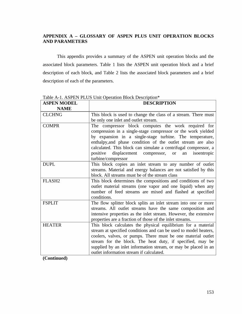
153

APPENDIX A – GLOSSARY OF ASPEN PLUS UNIT OPERATION BLOCKS AND PARAMETERS

This appendix provides a summary of the ASPEN unit operation blocks and the

associated block parameters. Table 1 lists the ASPEN unit operation block and a brief

description of each block, and Table 2 lists the associated block parameters and a brief

description of each of the parameters.

Table A-1. ASPEN PLUS Unit Operation Block Description* ASPEN MODEL

NAME DESCRIPTION

CLCHNG This block is used to change the class of a stream. There must be only one inlet and outlet stream.

COMPR The compressor block computes the work required for compression in a single-stage compressor or the work yielded by expansion in a single-stage turbine. The temperature, enthalpy,and phase condition of the outlet stream are also calculated. This block can simulate a centrifugal compressor, a positive displacement compressor, or an isoentropic turbine/compressor

DUPL This block copies an inlet stream to any number of outlet streams. Material and energy balances are not satisfied by this block. All streams must be of the stream class

FLASH2 This block determines the compositions and conditions of two outlet material streams (one vapor and one liquid) when any number of feed streams are mixed and flashed at specified conditions.

FSPLIT The flow splitter block splits an inlet stream into one or more streams. All outlet streams have the same composition and intensive properties as the inlet stream. However, the extensive properties are a fraction of those of the inlet streams.

HEATER This block calculates the physical equilibrium for a material stream at specified conditions and can be used to model heaters, coolers, valves, or pumps. There must be one material outlet stream for the block. The heat duty, if specified, may be supplied by an inlet information stream, or may be placed in an outlet information stream if calculated.

(Continued)

154

Table A-1. (Concluded)

ASPEN MODEL NAME

DESCRIPTION

MIXER This block simulates the mixing of two or more material and/or information streams. Every substream that appears in any outlet stream must be present in the inlet stream. The information stream can be either class “HEAT” or “WORK”. The user can specify the outlet pressure drop, the number of phases in the conventional substream, and the key phase.

PUMP This block is used to raise the pressure of an inlet stream to a specified value and calculates the power requirement. Alternatively PUMP will calculate the pressure of an outlet stream, given the inlet stream conditions and input work. This block can be used to model a centrifugal pump, a slurry pump, or a positive displacement pump.

RSTOIC This stoichiometric block can be used to simulate a reactor when the stoichiometry is known, but the reaction kinetics are unknown or unimportant. The model may have any number of inlet material streams and one outlet material stream. This block can handle any number of reactions.

SEP2 This block simulates separation processes when the details of a separation process are not relevant or available. All streams must be of the same stream class. The first outlet is the top stream, and the second is the bottom stream.

SEP This block separates an inlet stream into two or more outlet streams according to the split specified for each component. Two of the three properties, temperature, pressure, and vapor fraction, may be specified for each component.

RGIBBS This block computes the phase and/or chemical equilibrium compositions at user-specified temperature and pressure when any number of feed streams are mixed. The output consists of up to one vapor phase, any number of liquid and solid phases. All materials must be of same class, and all information streams must be of the class “HEAT”.

ABSBR This block determines the overhead vapor and bottom liquid streams given at a set of inlet streams with specified inlet tray locations, number of stages and sidedraws. The model allows two to five material inlets and two to five material outlet. All material streams must be of the same stream class. All information streams must be of class “HEAT”. The first material outlet is the top product stream. The second material outlet is the bottom product stream.

*Adapted from Akunuri (1999)

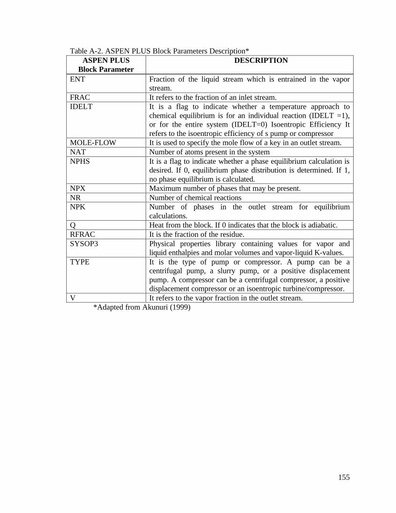
155

Table A-2. ASPEN PLUS Block Parameters Description* ASPEN PLUS

Block Parameter DESCRIPTION

ENT Fraction of the liquid stream which is entrained in the vapor stream.

FRAC It refers to the fraction of an inlet stream. IDELT It is a flag to indicate whether a temperature approach to

chemical equilibrium is for an individual reaction (IDELT =1), or for the entire system (IDELT=0) Isoentropic Efficiency It refers to the isoentropic efficiency of s pump or compressor

MOLE-FLOW It is used to specify the mole flow of a key in an outlet stream. NAT Number of atoms present in the system NPHS It is a flag to indicate whether a phase equilibrium calculation is

desired. If 0, equilibrium phase distribution is determined. If 1, no phase equilibrium is calculated.

NPX Maximum number of phases that may be present. NR Number of chemical reactions NPK Number of phases in the outlet stream for equilibrium

calculations. Q Heat from the block. If 0 indicates that the block is adiabatic. RFRAC It is the fraction of the residue. SYSOP3 Physical properties library containing values for vapor and

liquid enthalpies and molar volumes and vapor-liquid K-values. TYPE It is the type of pump or compressor. A pump can be a

centrifugal pump, a slurry pump, or a positive displacement pump. A compressor can be a centrifugal compressor, a positive displacement compressor or an isoentropic turbine/compressor.

V It refers to the vapor fraction in the outlet stream. *Adapted from Akunuri (1999)

156

APPENDIX B – ASPEN PLUS ENTHALPY CALCULATION

In order to verify the energy balance in an ASPEN PLUS simulation, a case study

was completed to test the methods that the program utilizes. Though ASPEN PLUS has

an extensive database of thermodynamic and physical properties for numerous chemical

compounds, there are many compounds that are so vaguely defined that it is not possible

to utilize a specific set of properties. Coal is an example of such a compound. If a

component is not in the ASPEN PLUS database, it is a non-conventional component.

ASPEN PLUS is unable to process non-conventional components in phase or chemical

equilibrium calculations. The only properties that are calculated for non-conventional

components are enthalpy and density (ASPEN PLUS Manual, 1996).

Non-conventional components are defined in ASPEN PLUS through component

attributes. Component attributes represent composition through one or more sets of

constituents. In the case of coal, the user can define the compound through an analysis of

the component such as ultimate, proximate and sulfur analyses. The ultimate analysis

characterizes the component in terms of carbon, hydrogen, sulfur, oxygen, nitrogen and

ash on a moisture-free weight percent basis. A proximate analysis characterizes the

component by the fixed carbon, volatile matter, ash and moisture weight percents. The

sulfur analysis characterizes the sulfur that a component contains by sulfur, pyritic and

organic (Thorsness, 1995).

Flow Sheet

The flow sheet developed for this case study is shown in Figure B-1. The model

consists of two reactors, an RYIELD and RSTOICH reactor. The RYIELD reactor is

used to break the fuel down to conventional components and the RSTOICH reactor is

used as a combustor.

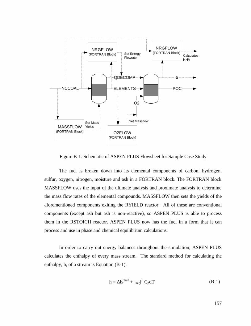
157

Figure B-1. Schematic of ASPEN PLUS Flowsheet for Sample Case Study

The fuel is broken down into its elemental components of carbon, hydrogen,

sulfur, oxygen, nitrogen, moisture and ash in a FORTRAN block. The FORTRAN block

MASSFLOW uses the input of the ultimate analysis and proximate analysis to determine

the mass flow rates of the elemental compounds. MASSFLOW then sets the yields of the

aforementioned components exiting the RYIELD reactor. All of these are conventional

components (except ash but ash is non-reactive), so ASPEN PLUS is able to process

them in the RSTOICH reactor. ASPEN PLUS now has the fuel in a form that it can

process and use in phase and chemical equilibrium calculations.

In order to carry out energy balances throughout the simulation, ASPEN PLUS

calculates the enthalpy of every mass stream. The standard method for calculating the

enthalpy, h, of a stream is Equation (B-1):

h = ∆hfTref + Tref∫T CpdT (B-1)

ELEMENTSNCCOAL

QDECOMP 5

POC

O2

Set MassYieldsMASSFLOW

(FORTRAN Block)

Set EnergyFlowrate

NRGFLOW(FORTRAN Block)

O2FLOW(FORTRAN Block)

Set Massflow

NRGFLOW(FORTRAN Block)

CalculatesHHV

158

where ∆hfTref is the heat of formation of the component at a reference temperature (Tref)

and Cp is its specific heat capacity. The enthalpy is calculated for all the components of a

stream and the sum of all the enthalpies is the total stream enthalpy. If the stream

consists of all conventional components, the enthalpy of the stream is easily calculated by

ASPEN PLUS. However, for non-conventional components, ASPEN PLUS cannot

calculate the enthalpy of the stream via this method. Instead, the heat of combustion is

used to calculate the heat of formation, as in Equation (B-2):

∆hfTref = ∆hc

Tref + ∑ ∆hfTref (B-2)

where ∆hcTref is the heat of combustion of the non-conventional component and the

summation is the heat of formation of the combustion products at a reference

temperature. Specifically, ASPEN PLUS uses Equation (B-3) to calculate the heat of

formation from the heat of combustion.

∆hf = ∆hc –(1.418x106wHd + 3.278x106wC

d + 9.264x104wSd –2.418x106wN

d –1.426x104wCl

d) 102 (B-3)

where w is the weight percent, the superscript d specifies dry basis, subscripts H, C, S, N

and Cl note hydrogen, carbon, sulfur, nitrogen and chlorine, respectively (ASPEN PLUS

Manual, 1996).

The heat capacity for a non-conventional component is calculated by the Kirov

correlation. The Kirov correlation regards coal as a mixture of moisture, ash, fixed

carbon and primary and secondary volatile matter. The correlation treats the heat

capacity as weighted sums of these constituents. The Kirov correlation is shown in

Equation (B-4).

Cpd = Σwj(aj1 + aj2T + aj3T

2 + aj4T3) (B-4)

where Cpd is the heat capacity on a dry basis, a are coefficients for the constituents,

subscript j is the constituent index, w is the mass fraction of the constituent on a dry

basis, and T is the temperature in Kelvin.

159

ASPEN PLUS allows the user to specify the ∆hcTref for a non-conventional

component on a dry basis. If the ∆hcTref is not available, there are five correlations

ASPEN PLUS can use to predict the heat of combustion of a non-conventional

component: the Boie, Mott and Spooner, Grummel and Davis, IGT, and Dulong

correlations (ASPEN PLUS Manual, 1996). In this simulation, the user specifies the heat

of combustion. The Dulong correlation is used to determine the heating value of the

American waste fuel, as described in Section 6.1. The Dulong equation is provided in

Equation (B-5):

∆hcTref = (145.44wC + 620.28wH + 40.5wS –77.54wO –16.0wN)102 –16.0 (B-5)

where,

wC = weight fraction of Carbon on a dry, ash free basis

wH = weight fraction of Hydrogen on a dry, ash free basis

wS = weight fraction of Sulfur on a dry, ash free basis

wO = weight fraction of Oxygen on a dry, ash free basis

wN = weight fraction of Nitrogen on a dry, ash free basis

After the FORTRAN block MASSFLOW has been completed and the fuel has

been decomposed into its elements, ASPEN PLUS calculates the enthalpy of the stream

based on the data in it’s database for carbon, hydrogen, sulfur, oxygen, nitrogen and

moisture. The enthalpy of the elemental coal stream is not the same as the enthalpy of

the non-conventional coal stream. Therefore, in order to maintain the energy balance, a

FORTRAN block is used to determine the difference in enthalpy of the two streams.

This difference is added back to the system through the heat stream QDECOMP to the

RSTOICH block. The FORTRAN block that calculates this difference and maintains the

energy balance is NRGFLOW.

There is also a FORTRAN block, O2FLOW, which determines the stoichiometric

amount of oxygen that is supplied to the RSTOICH reactor for complete combustion of

the fuel. A final FORTRAN block, HVCALC, is used to calculate the heat of

160

combustion. The block calculates the heat of combustion by dividing the heat coming

out of the RSTOICH reactor by the coal mass flowrate. The result is the coal’s heat of

combustion.

The RYIELD reactor is specified at a temperature of 25 °C and a pressure of 1

atmosphere. The FORTRAN block MASSFLOW sets the mass fractions yields for the

reactor. The RSTOICH is also specified at a temperature of 25 °C and a pressure of 1

atmosphere. Additionally, the following reactions described by Equations (B-6) to (B-9):

C + O2 à CO2 (B-6)

2 H2 + O2 à 2 H2O (B-7)

S + O2 à SO2 (B-8)

N2 +.5 O2 à NO2 (B-9)

Furthermore, the reactor is specified so that the water in the exhaust is in liquid

form, providing the resultant heat of combustion calculation to be the higher heating

value.

Case Study

Two case studies were done using this model with two different coals as fuels:

Illinois #6 and Pittsburgh #8. The compositions of the coals are shown in Table B-1.

Both coals were specified at an inlet standard temperature and pressure (25 °C, 1 ATM)

and a flow rate of 560,780 lb/hr. The results of each coal are given in Table B-2.

Comparing the heating values calculated from the ASPEN PLUS simulation of

Table B-2 to the heating values specified in Table B-1, the simulation seems to

miscalculate the value. However, the heating value of Table B-1 is on a dry basis and the

value calculated in Table B-2 contains moisture. This is proven, using Illinois #6 coal as

an example, in Equation (B-10).

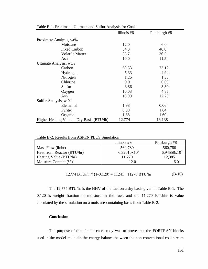
161

Table B-1. Proximate, Ultimate and Sulfur Analysis for Coals

Illinois #6 Pittsburgh #8

Proximate Analysis, wt% Moisture 12.0 6.0 Fixed Carbon 54.3 46.0 Volatile Matter 35.7 36.5 Ash 10.0 11.5

Ultimate Analysis, wt% Carbon 69.53 73.12 Hydrogen 5.33 4.94 Nitrogen 1.25 1.38 Chlorine 0.0 0.09 Sulfur 3.86 3.30 Oxygen 10.03 4.85 Ash 10.00 12.23

Sulfur Analysis, wt% Elemental 1.98 0.06 Pyritic 0.00 1.64 Organic 1.88 1.60

Higher Heating Value – Dry Basis (BTU/lb) 12,774 13,138

Table B-2. Results from ASPEN PLUS Simulation

Illinois # 6 Pittsburgh #8 Mass Flow (lb/hr) 560,780 560,780 Heat from Reactor (BTU/hr) 6.32010x109 6.94558x109 Heating Value (BTU/hr) 11,270 12,385 Moisture Content (%) 12.0 6.0

12774 BTU/hr * (1-0.120) = 11241 ≅11270 BTU/hr (B-10)

The 12,774 BTU/hr is the HHV of the fuel on a dry basis given in Table B-1. The

0.120 is weight fraction of moisture in the fuel, and the 11,270 BTU/hr is value

calculated by the simulation on a moisture-containing basis from Table B-2.

Conclusion

The purpose of this simple case study was to prove that the FORTRAN blocks

used in the model maintain the energy balance between the non-conventional coal stream

162

and the elemental conventional stream. An additional purpose of the study was to

confirm that the method of allowing the user to input the heat of combustion value of the

fuel is an acceptable means of specifying the enthalpy of the coal.

The simulation was conducted at standard temperature and pressure and complete

combustion of the fuel was specified. It is expected that the heat from the combustion

divided by the mass of the fuel will yield the higher heating value of the fuel. The results

from Table B-2 confirm this. The only difference between the results from Table B-2

and the input specification of Table B-1 is that the input is on a dry basis and the

calculation from Table B-2 is on a moisture-containing basis. Therefore the method used

for managing the energy balance between the conventional and non-conventional

components is legitimate.