ABSTRACT HONG, TAO. Short Term Electric Load Forecasting

ABSTRACT

HONG, TAO. Short Term Electric Load Forecasting. (Under the direction of Simon Hsiang and Mesut Baran).

Load forecasting has been a conventional and important process in electric utilities since the

early 20th century. Due to the deregulation of the electric utility industry, the utilities tend to

be conservative about infrastructure upgrade, which leads to stressed utilization of the

equipment. Consequently, the traditional business needs of load forecasting, such as

planning, operations and maintenance, become more crucial than before. In addition,

participation in the electricity market requires the utilities to forecast their loads accurately.

Nowadays, with the promotion of smart grid technologies, load forecasting is of even greater

importance due to its applications in the planning of demand side management, electric

vehicles, distributed energy resources, etc.

In today’s practice, many business areas of the utilities produce their own load forecasts,

which results in the inefficient and ineffective use of resources. This dissertation proposes an

integrated forecasting framework with the concentration on the short term load forecasting

(STLF) engine that can easily link to various other forecasts. Although dozens of techniques

have been developed, studied, and applied to STLF, there are still many challenging issues in

the field, such as lack of benchmark and the systematic approach of building the STLF

models. This dissertation disassembles the major techniques that have been applied to STLF

and reported in the literature, and reassembles the key elements to come up with a

methodology to analyze STLF problems and develop STLF models. Multiple linear

regression (MLR) analysis, as one of the earliest and widest applied techniques for STLF, is

deployed in the case study of a US utility. The resulting models have outperformed the

forecasts developed by several other internal and external parties and been in production use

since 2009 with excellent performance. Through the presented study, the knowledge of

applying MLR to STLF has been advanced by bringing in interaction effects. Meanwhile, a

benchmarking model is developed for a wide range of utilities. Furthermore, possibilistic

linear regression, as one of the emerging techniques in the field of STLF, is investigated,

compared with MLR, and enhanced for the STLF application. Since artificial neural

networks (ANN) have been popular in the STLF research community over the past two

decades, several ANN based models are also developed for comparative assessment.

Short Term Electric Load Forecasting

by Tao Hong

A dissertation submitted to the Graduate Faculty of North Carolina State University

in partial fulfillment of the requirements for the degree of

Doctor of Philosophy

Operations Research and Electrical Engineering

Raleigh, North Carolina

9/10/2010

APPROVED BY:

_______________________________ ______________________________ Simon M Hsiang Mesut E Baran Committee Chair Committee Co-chair _______________________________ ______________________________ Shu-Cherng Fang David A Dickey

ii

Dedication

To Baohui Yin, Jinmin Hong, and Pu Wang,

iii

Biography Tao Hong received his Bachelor of Engineering degree in Automation from Tsinghua

University, Beijing in July 2005, his Master of Science degree in Electrical

Engineering, and his second Master of Science degree with co-majors in Operation

Research and Industrial Engineering from North Carolina State University in May

2008 and Dec 2008 respectively.

iv

Acknowledgements As a graduate student who has gone through 5 years of graduate school with nearly

40 courses across 7 programs, I’ve seen too many peers suffering with the following

Q&A’s:

Q: Why PhD?

A: I have no choice. I can’t find a job.

Q: Why this research topic?

A: I have no choice. My advisor asked me to work on it.

Fortunately, I have been enjoying the academic freedom in my graduate study. I had

choices to stay in or quit my first PhD program in electrical engineering, and I quit. I

had choices to select the major of my second master degree from a wide range of

disciplines, such as operations research, statistics, computer science, mathematics and

industrial engineering, and I chose OR and IE. I had choices to stay in school for PhD

or start a full-time job in a leading utility consulting firm, and I chose to pursue my

PhD. Since then I had the freedom to focus on the research topic I’m interested in, to

form the committee that have, in my opinion, the brightest brains in the related fields.

All of these are granted by the people around me, such as my wife, my parents, my

advisor, my committee members and the graduate program of operations research,

etc.

v

Dr. Simon Hsiang, who was master thesis advisor and now my PhD advisor, is the

first one to educate me what the meaning of Ph.D. is. Although the research direction

I finally decided to go to is not what he is interested in, he still offered me tremendous

constructive comments and insights, of which “As long as it’s good science” has

always been his justification. Thank Dr. Hsiang for granting me total freedom all the

way. It’s also my fortune that Dr. Hsiang trusts my capability, which cannot be more

encouraging to me during my research.

Dr. Mesut Baran is the first one to lead me to the field of power systems. I highly

appreciate his course ECE550, the first power systems course I took, which helped

build my fundamental background of power system analysis. Also many thanks to Dr.

Baran for the suggestion of putting ANN into the comparative assessment, which

made the dissertation as well rounded as it is now.

Dr. Shu-Cherng Fang, a perfect example for my life, taught me optimization theory

from linear programming, nonlinear programming, to soft computing. I’m so glad that

I took three of his courses, while I regret that I was not able to take more. I’m so

proud that I passed my qualify exam with him as one of the examination committee

members, while I regret that I didn’t do better to get a high pass. Thanks Dr. Fang for

accepting me as one of the FANGroup members, which allows me to listen to his

advice every week. Special thanks to him for pointing me how thousands of junky

vi

papers were produced by irresponsible researchers, and keeping me from being one of

them.

Dr. Dickey is the first one to introduce me to time series analysis. The first time I

took his lecture, I said to myself: “This subject has to be appreciated by the load

forecasting guys in the way he presented.” It’s my honor to have Dr. Dickey on my

committee. I will always be grateful that there has been a Nobel citation professor

who read my dissertation draft word-by-word and offered the revision comments in

great detail.

Dr. Richard Brown, the greatest boss I’ve ever experienced, is the first one to bring

me to the utility industry, and also the first person that encouraged me to pursue a

degree in OR. It’s so unfortunate that he was not able to attend my final oral exam.

However, my research wouldn’t be as valuable as it is to the industry without Dr.

Brown’s advice since day one. I also greatly appreciate the career guidance and

flexible working environment he offered me.

There are many other people who offered me significant amount of help during the

past two years. Dr. Carl Meyer helped me build a solid background in matrix analysis

and applied linear algebra. Dr. Le Xu worked with me in the very early stage to

develop the models for short term load forecasting. Mr. Robert Bisson awarded the

integrated load forecasting project to us and encouraged me to get my PhD out of it.

Dr. Min Gui and Mr. H. Lee Willis worked with me on the technical development

vii

portion of this priceless project, of which most materials became part of the contents

in this dissertation.

Lastly, but the most importantly, I would like to express my deepest appreciation to

my family. My wife, Pu Wang, originally had the idea of applying the full version of

multiple linear regression to short term load forecasting. It was amazing to see that

the preliminary model we built in two days beat the ones developed by several other

parties for months and years. Her help with some implementations, as well as the

support in the daily life, made the miracle of my 20-month PhD happen. Thanks to

my parents, Baohui Yin and Jinmin Hong, for their financial support that enabled me

to spend most of my time concentrating on my research, and strong encouragement

that pushed me to fearlessly pursue my PhD degree.

viii

Table of Contents List of Tables .............................................................................................................. xii

List of Figures ............................................................................................................. xv

1 Introduction ........................................................................................................... 1

1.1 FORECASTING IN ELECTRIC UTILITIES .................................................................................................. 2

1.2 BUSINESS NEEDS OF LOAD FORECASTS ............................................................................................... 3

1.3 CLASSIFICATION OF LOAD FORECASTS ................................................................................................. 6

1.4 INTEGRATED FORECASTING WITH A STLF ENGINE ............................................................................... 10

2 Literature Review ................................................................................................ 14

2.1 OVERVIEW .................................................................................................................................. 15

2.2 REVIEW OF THE LITERATURE REVIEWS .............................................................................................. 18

2.2.1 Conceptual Reviews ....................................................................................................... 18

2.2.2 Experimental Reviews .................................................................................................... 23

2.3 STATISTICAL APPROACHES.............................................................................................................. 25

2.3.1 Regression Analysis ....................................................................................................... 25

2.3.2 Time Series Analysis ....................................................................................................... 28

2.4 ARTIFICIAL INTELLIGENCE TECHNIQUES ............................................................................................. 31

2.4.1 Artificial Neural Networks ............................................................................................. 31

2.4.2 Fuzzy Logic ..................................................................................................................... 36

2.4.3 Fuzzy Neural Network .................................................................................................... 39

2.4.4 SVM and Others ............................................................................................................. 41

ix

2.5 WEATHER VARIABLES ................................................................................................................... 43

2.6 CALENDAR VARIABLES ................................................................................................................... 45

2.7 BIBLIOGRAPHY ............................................................................................................................. 48

2.8 SUMMARY .................................................................................................................................. 53

3 Theoretical Background ...................................................................................... 55

3.1 MULTIPLE LINEAR REGRESSION ....................................................................................................... 56

3.1.1 General Linear Regression Models ................................................................................ 56

3.1.2 Quantitative and Qualitative Predictor Variables ......................................................... 57

3.1.3 Polynomial Regression ................................................................................................... 59

3.1.4 Transformed Variables .................................................................................................. 60

3.1.5 Interaction Effects .......................................................................................................... 61

3.1.6 Linear Model vs. Linear Response Surface ..................................................................... 62

3.2 POSSIBILISTIC LINEAR REGRESSION .................................................................................................. 63

3.2.1 Background .................................................................................................................... 63

3.2.2 Possibilistic Linear Models ............................................................................................. 66

3.3 ARTIFICIAL NEURAL NETWORKS ...................................................................................................... 69

3.4 DIAGNOSTIC STATISTICS ................................................................................................................ 72

4 Multiple Linear Regression for Short Term Load Forecasting ........................... 76

4.1 BENCHMARK ............................................................................................................................... 77

4.1.1 Motivation ..................................................................................................................... 77

4.1.2 Evaluation criterion ....................................................................................................... 79

4.1.3 Benchmarking Model ..................................................................................................... 81

4.2 EXTENSIONS OF GLMLF‐B ............................................................................................................ 91

x

4.2.1 VSTLF with Preceding Hour Load ................................................................................... 91

4.2.2 MTLF/LTLF with Economics ............................................................................................ 92

4.3 CUSTOMIZATION .......................................................................................................................... 93

4.3.1 Recency Effect ................................................................................................................ 93

4.3.2 Weekend Effect .............................................................................................................. 97

4.3.3 Holiday Effect ............................................................................................................... 101

4.3.4 Exponentially Weighted Least Squares ........................................................................ 110

4.3.5 Results ......................................................................................................................... 111

4.4 IMPACT OF DEMAND SIDE MANAGEMENT TO LOAD FORECASTING ACCURACY ....................................... 116

5 Possibilistic Linear Model Based Load Forecasters ......................................... 119

5.1 BENCHMARKING MODEL ............................................................................................................. 120

5.2 IMPACT OF DEMAND SIDE MANAGEMENT TO FORECASTING ACCURACY ............................................... 122

5.3 NUMERICAL EXAMPLES ............................................................................................................... 124

5.3.1 Data ............................................................................................................................. 124

5.3.2 PLM Underperforms GLM ............................................................................................ 126

5.3.3 PLM Outperforms GLM ................................................................................................ 129

5.3.4 PLM ties with GLM ....................................................................................................... 131

5.4 SUMMARY AND DISCUSSION ........................................................................................................ 134

6 Artificial Neural Networks Based Load Forecasters ........................................ 136

6.1 SINGLE MODEL FORECASTING ...................................................................................................... 137

6.2 MULTI‐MODEL FORECASTING ....................................................................................................... 141

6.3 COMPARISON WITH GLMLFS ....................................................................................................... 143

7 Conclusion ........................................................................................................ 146

xi

8 References ......................................................................................................... 148

xii

List of Tables Table 1.1 Needs of forecasts in utilities. ....................................................................... 5

Table 1.2 Availability of temperature, economics, and land use information. ............. 9

Table 1.3 Classification of load forecasts. .................................................................... 9

Table 1.4 Applications of the forecasts. ........................................................................ 9

Table 2.1 Day type codes appeared in the literature. .................................................. 47

Table 3.1 Conceptual differences between MLR and PLR ........................................ 64

Table 4.1 Benchmark candidates ................................................................................ 89

Table 4.2 MAPEs of the seven benchmarking model candidates. .............................. 90

Table 4.3 MAPEs of the Recency Effect Candidates ................................................. 96

Table 4.4 MAPEs of the Weekend Effect Candidates .............................................. 100

Table 4.5 US Public Holidays Established by Federal Law (5 U.S.C. 603) ............. 102

Table 4.6 MAPEs of the Alternatives for the Six Fix-Weekday Holidays ............... 107

Table 4.7 MAPEs of the Alternatives for the Surrounding Days of Memorial Day and

Labor Day ................................................................................................................. 107

Table 4.8 MAPEs of the Alternatives for the Four Fix-Date Holidays .................... 108

Table 4.9 MAPEs of the Days After the Three Significant Fix-Date Holidays ....... 108

Table 4.10 GLMLF-HT vs. GLMLF-TW .................................................................. 109

Table 4.11 MAPEs of the Exponentially Weighted Least Squares Candidates ....... 110

xiii

Table 4.12 MAPEs of the five milestone models ..................................................... 111

Table 4.13 One Week Ahead Forecasting Performance for All Milestones ............. 112

Table 4.14 Effectiveness of Holiday Effect Modeling of GLMSTLF-HT ................ 113

Table 4.15 MAPEs of GLMSTLF-HT in Special Hours ........................................... 115

Table 4.16 DSM activities (2001 – 2008) ................................................................. 116

Table 4.17 MAPEs of the Five Milestone Models (Preprocessed Data). ................. 117

Table 4.18 One Week Ahead Forecasting Performance Comparison (GLMSTLF-HT)

................................................................................................................................... 118

Table 5.1 MAPEs of the seven PLM based benchmarking model candidates. ........ 120

Table 5.2 MAPEs of the seven PLM based benchmarking model candidates

(preprocessed data). .................................................................................................. 123

Table 5.3 Data for numerical examples. ................................................................... 124

Table 5.4 Seven numerical examples. ....................................................................... 133

Table 6.1 MAPEs of ANNLF-S. ................................................................................ 138

Table 6.2 MAPEs of ANNLF-BS. ............................................................................. 139

Table 6.3 MAPEs of ANNLF-HTS............................................................................ 140

Table 6.4 MAPEs of ANNLF-BM. ............................................................................ 141

Table 6.5 MAPEs of ANNLF-HTM. ......................................................................... 142

Table 6.6 One Year Ahead Forecasting Performance for All ANNLFs .................... 145

xiv

Table 6.7 One Year Ahead Forecasting Performance for GLMLF-B and GLMLF-HT

................................................................................................................................... 145

xv

List of Figures Figure 1.1 Organization of the dissertation................................................................. 13

Figure 2.1 A typical STLF process. ............................................................................ 15

Figure 3.1 A three-layer feed-forward artificial neural network. ............................... 71

Figure 4.1 Load series (2005-2008). ........................................................................... 83

Figure 4.2 Temperature series (2005-2008). ............................................................... 83

Figure 4.3 Load-temperature scatter plot (2005-2008). .............................................. 84

Figure 4.4 Load-temperature scatter plots for 12 months. .......................................... 86

Figure 4.5 Load-temperature scatter plots (Hours 1 to 12). ........................................ 87

Figure 4.6 Load-temperature scatter plots (Hours 13 to 24). ...................................... 88

Figure 4.7 Normalized hourly load profile of a week. .............................................. 100

Figure 4.8 The annual peak day of 2009. .................................................................. 115

Figure 5.1 Data for the numerical examples. ............................................................ 125

Figure 5.2 Example 1: PLM underperforms GLM. .................................................. 127

Figure 5.3 Example 2: PLM underperforms GLM. .................................................. 128

Figure 5.4 Example 3: PLM outperforms GLM. ...................................................... 129

Figure 5.5 Example 4: PLM outperforms GLM. ...................................................... 130

Figure 5.6 Example 5: PLM ties with GLM. ............................................................ 131


xvi


1

1 Introduction

Formal planning and forecasting approaches, which have been used in business,

government, and nonprofit organizations since 1950s, are shown to be valuable to the

organizations [4]. In the electric utility industry, many big utilities have their in-house

load forecasting capability, while the small ones may have to outsource the load

forecasting processes due to the high cost of time and materials. Nevertheless, as a

utility grows up to a certain size, it may become economically justifiable to perform

in-house load forecasting. This chapter discusses the current practices in the electric

utility industry, introduces the concepts and fundamentals of electric load forecasting,

and proposes a new approach for modern utilities to perform load forecasting tasks.

2

1.1 Forecasting in Electric Utilities

In many organizations, planning and forecasting are seamlessly integrated together.

Therefore, the forecasting function of a utility is normally assigned to the planning

department. Nevertheless, the distinction between the two should not be omitted.

Planning provides the strategies, given certain forecasts, whereas forecasting

estimates the results, given the plan. Planning relates to what the utility should do.

Forecasting relates to what will happen if the utility tries to implement a given

strategy in a possible environment. Forecasting also helps to determine the likelihood

of the possible environments.

Traditionally, a department is in charge of the specific forecasts it needs, which

includes assigning job positions for the engineers, gathering necessary data, etc. This

process does not require much communication among the various departments, which

leads to two drawbacks. Firstly, resources are not efficiently utilized. For instance, the

same forecast may be produced by two departments independently. Secondly, the

quality of the forecasts may vary a lot. For instance, the trading department may use

the billing data to produce the one-day-ahead forecast, while the planning department

may use supervisory control and data acquisition (SCADA) data for the same

purpose. Consequently, the accuracy difference between the billing data and SCADA

data would lead to different quality of the forecasts.

3

1.2 Business Needs of Load Forecasts

In today’s world, load forecasting is an important process in most utilities with the

applications spread across several departments, such as planning department,

operations department, trading department, etc. The business needs of the utilities can

be summarized, but not limited to, the following:

1) Energy purchasing. Whether a utility purchases its own energy supplies from

the market place, or outsources this function to other parties, load forecasts are

essential for purchasing energy. The utilities can perform bi-lateral purchases

and asset commitment in the long term, e.g., 10 years ahead. They can also do

hedging and block purchases one month to 3 years ahead, and adjust (buy or

sell) the energy purchase in the day-ahead market.

2) Transmission and distribution (T&D) planning [90]. The utilities need to

properly maintain and upgrade the system to satisfy the growth of demand in

the service territory and improve the reliability. And sometimes the utilities

need to hedge the real estate to place the substations in the future. The

planning decisions heavily rely on the forecasts, known as spatial load

forecasts, that contain when, where, and how much the load as well as the

number of customers will grow.

4

3) Operations and maintenance. In daily operations, load patterns obtained

during the load forecasting process guide the system operators to make

switching and loading decisions, and schedule maintenance outages.

4) Demand side management (DSM). Although lots of DSM activities are belong

to daily operations, it is worthwhile to separate DSM from the operations

category due to its importance in this smart-grid world. A load forecast can

support the decisions in load control and voltage reduction. On the other hand,

through the studies performed during load forecasting, utilities can perform

long term planning according to the characteristics of the end-use behavior of

certain customers.

5) Financial planning. The load forecasts can also help the executives of the

utilities project medium and long term revenues, make decisions during

acquisitions, approve or disapprove project budgets, plan human resources

and technologies, etc.

According to the lead time range of each business need described above, the

minimum updating cycle and maximum horizon of the forecasts are summarized in

Table 1.1.

5

Table 1.1 Needs of forecasts in utilities.

Minimum updating cycle Max horizon Energy purchasing 1 hour 10 years and above

T&D planning 1 day 30 years Operations 15 minutes 2 weeks

DSM 15 minutes 10 years and above Financial planning 1 month 10 years and above

6

1.3 Classification of Load Forecasts

There is no single forecast that can satisfy all of the needs of utilities. A common

practice is to use different forecasts for different purposes. The classification of

various forecasts is not only depending upon the business needs of utilities, but also

the availability of the crucial elements that affect the energy consumption: weather

(or climate in the long periods) and human activities.

Weather refers to the present condition of the meteorological elements, such as

temperature, humidity, wind, rainfall, etc., and their variations in a given region over

periods up to two weeks. Climate encompasses these same elements in a given region

and their variations over long periods of time. The uses of various weather variables

will be discussed in the next chapter. Since temperature has the most impact to energy

consumption among all the meteorological elements, all the models developed in this

report use temperature information only. Nevertheless, the methodology can be

applied to other meteorological elements. Nowadays, for load forecasting purpose,

temperature forecast can be relatively accurate up to one day ahead, and be inaccurate

but reliable up to two weeks ahead.

The impact of human activities to energy consumption can be realized in several

aspects. In the hourly resolution, the impact varies over the calendar variables

including day of the week, and month of the year. The calendar information is

normally certain for the next decade. In the monthly or quarterly resolution, the

7

impact varies on different economical conditions. For instance, during the year of

2009, which is the early part of a recession in US, the energy consumption of US is

lower than that of 2008, because people were using power more conservatively, and

lots of businesses were closed. With the advancement of econometric techniques, the

economics information can be relatively accurate up to one year ahead, and be

inaccurate but reliable up to 3 years ahead for load forecasting purpose. In the annual

resolution, both climate and economics can affect the energy consumption. However,

due to the unavailability of both inputs, the system level load forecast can be only

obtained by simulating various scenarios. On the other hand, the long term energy

consumption on the circuit level is affected by urban development, which can be

realized by land use changes. The land use information is normally accurate within

one year, inaccurate but reliable up to 5 years. Although some counties can provide a

30 years ahead urban development plan, it is still not clear what exactly would

happen year by year during the next 30 years. Forecasting the load on the circuit level

with land use simulation is called spatial electric load forecasting [89].

Table 1.2 summarizes the availability of temperature, economics, and land use

information for load forecasting purposes. Consequently, Table 1.3 shows one way to

classify the various load forecasts according to the availability of input information,

the updating cycle and horizon: very short term load forecasting (VSTLF), short term

8

load forecasting (STLF), medium term load forecasting (MTLF), and long term load

forecasting (LTLF).

In VSTLF, temperature, economics and land use information can all be optional,

because the load in the near future can be forecasted by the load in the past. Since

both economics and land use information are relatively stable (unchanged) in the

short time span (less than 2 weeks), they can be optional in STLF. On the other hand,

the temperature information plays a key role in STLF. Decisions such as how much

power to purchase should be made based on the distribution of the load forecast

which is driven by the distribution of temperature forecast. In MTLF, temperature

cannot be predicted accurately for the coming 3 years. Therefore, simulated scenarios

of temperature based on the local temperature history can be used in the model. While

the economics is predictable and affects the mid-term load consumption, it is required

in MTLF. Land use information is optional in VSTLF, STLF, and MTLF because the

land use could barely change a lot during a 3-year horizon. However, in the long

term, land use change is the major factor that drives the load. Therefore, land use

information is required in LTLF. On the other hand, temperature and economics

information is hard to predict in the long run, the simulated scenarios can be used.

9

Table 1.2 Availability of temperature, economics, and land use information.

Accurate Inaccurate Unreliable Temperature 1 day 2 weeks > 2 week Economics 1 month 3 years > 3 years Land use 1 year 5 years > 5 years

Table 1.3 Classification of load forecasts.

Temperature Economics Land Use Updating Cycle Horizon VSTLF Optional Optional Optional <= 1 Hour 1 day STLF Required Optional Optional 1 Day 2 weeks MTLF Simulated Required Optional 1 month 3 years LTLF Simulated Simulated Required 1 year 30 years

With the classification of load forecasts shown in Table 1.3, we can associate each

forecast to the business needs of the utilities and the corresponding lead time, which

are shown in Table 1.4. Due to the wide span of updating cycle and horizon, one

business need may be tied to several forecasts. For instance, an energy purchasing

contract may be one day ahead, one year ahead, or 10 years ahead, where load

forecasts from very short term to long term can be applied.

Table 1.4 Applications of the forecasts.

VSTLF STLF MTLF LTLF Energy purchasing X X X X

T&D planning X X X Operations X X

DSM X X X X Financial planning X X

10

1.4 Integrated Forecasting with a STLF Engine

Although several departments in a utility may share the same type of forecasts,

usually there is not much communication among them in the current practice, which

results in inefficient utilization of resources. Not only are human resources used

redundantly, producing the same forecast in various departments, but also the quality

of these forecasts may vary due to the lack of communication and information

sharing. For instance, on STLF, operations department may use SCADA data, which

may not be as accurate as the billing data used by the trading department. On the

other hand, the trading department may not know about an ongoing outage, which

would result in a less accurate forecast for the next few hours.

This dissertation develops a novel regression-based STLF engine for an integrated

load forecasting process. The term “integrated” here refers to initiating all the

forecasts from the same department with the same methodology and engine. STLF is

selected as the engine and base of the integrated forecasting process due to its

inherent connectivity to other types of forecasts:

1) STLF to VSTLF: A STLF model can be transformed into a VSTLF model by

adding the loads of some preceding hours as part of the inputs to the STLF

model, which captures the autocorrelation of the current hour load and the

preceding hour loads. Alternatively, with the STLF as a base, residuals of

historical load can be collected and form a new series. Then by forecasting the

11

future residuals and adding them back to the short term forecast, a very short

term forecast can be obtained.

2) STLF to MTLF & LTLF: by adding econometrics variables to the STLF

model and extrapolating the model to the longer horizon, the system level

MTLF and LTLF can be obtained. Consequently, this long term system level

load forecast can be used as an input for long term spatial load forecasting.

The rest of this dissertation is mainly devoted to the STLF model development. The

organization of this dissertation is shown in Figure 1.1. Chapter 2 presents a

comprehensive literature review of STLF. Chapter 3 introduces the theoretical

background of three techniques, multiple linear regression (MLR) – one of the

earliest and most widely applied techniques in STLF, possibilistic linear regression

(PLR) – one of the most recently applied techniques in STLF, and artificial neural

networks (ANN) – one of the most popular techniques in STLF. Chapter 4 develops

several general linear model (GLM) based load forecasters1 starting from a base

model (GLMLF-B) for benchmarking purposes. The extensions of this base model are

demonstrated. Then it is customized by modeling several special effects. Chapters 5

and 6 develop the possibilistic linear models (PLMs) and ANNs for load forecasting

respectively. The focus is on the comparisons to the GLMs. Through the comparative

assessment, ways to utilize and improve PLR and ANN for STLF are discussed. The

1 The “load forecaster” in this dissertation, as well as many other papers in load forecasting, refers to the forecasting method rather than a person who performs load forecasting.

12

dissertation is concluded in Chapter 7 with the discussion of the possible extension of

the proposed research.

13

Figure 1.1 Organization of the dissertation.

14

2 Literature Review

Thousands of papers and reports were published in the load forecasting field in the

past 50 years. The literature review presented in this chapter concentrates on the

STLF literature published in the reputable journals. The papers are reviewed from

three aspects: the techniques developed or applied, the various variables deployed,

and the representative work done by several major research groups. The reviews tend

to be focused on the major development in the field rather than covering every aspect

of the matter. The comments to the papers in this review are addressed on the

conceptual level.

15

2.1 Overview

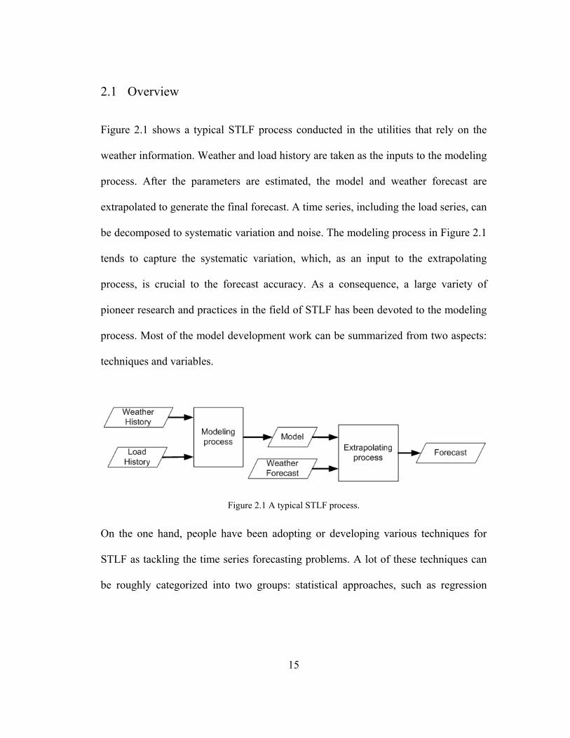
Figure 2.1 shows a typical STLF process conducted in the utilities that rely on the

weather information. Weather and load history are taken as the inputs to the modeling

process. After the parameters are estimated, the model and weather forecast are

extrapolated to generate the final forecast. A time series, including the load series, can

be decomposed to systematic variation and noise. The modeling process in Figure 2.1

tends to capture the systematic variation, which, as an input to the extrapolating

process, is crucial to the forecast accuracy. As a consequence, a large variety of

pioneer research and practices in the field of STLF has been devoted to the modeling

process. Most of the model development work can be summarized from two aspects:

techniques and variables.

Figure 2.1 A typical STLF process.

On the one hand, people have been adopting or developing various techniques for

STLF as tackling the time series forecasting problems. A lot of these techniques can

be roughly categorized into two groups: statistical approaches, such as regression

16

analysis [66] and time series analysis [28], and artificial intelligence (AI) based

approaches, such as ANN [31], fuzzy logic (FL) [74], and support vector machine

(SVM) [10]. Various combinations of these techniques have also been studied and

applied to STLF problems.

On the other hand, people have been seeking the most suitable variables for each

particular problem and trying to generalize the conclusions to interpret the causality

of the electric load consumption. Most of these efforts were embedded coherently

into the development of the techniques. For instance, temperature and relative

humidity were considered in [48], while The effect of humidity and wind speed were

considered through a linear transformation of temperature in the improved version

[49]. In general, the electric load is mainly driven by nature and human activities. The

effects of nature are normally reflected by weather variables, e.g., temperature, while

the effects of human activities are normally reflected by the calendar variables, e.g.,

business hours. The combined effects of both elements exist as well but are

nontrivial.

With the progress of deregulation, more and more parties have joined the energy

markets, where electricity is traded as a commodity. In some situations, the

consumers tend to shift electricity consumption from the expensive hours to other

times when possible. Price information would affect the load profiles in such a price-

sensitive environment. Following this thought, a price-sensitive load forecaster was

17

proposed, of which the results are reported to be superior to an existing STLF

program [50]. Since the price-sensitive environment is not generic in the current US

utility industry, price information was not included in Figure 2.1 or the scope of this

report.

Although the majority of the literature in STLF is on the modeling process, there is

some research concerning other aspects to improve the forecast. Weather forecast, as

an input to the extrapolating process, is also very important to the accuracy of STLF.

Consequently, another branch of research work is focusing on developing, improving

or incorporating the weather forecast [32]. A temperature forecaster is proposed for

STLF [47]. Front-end weather forecast is incorporated in the STLF system to improve

the forecasting performance [61].

The rest of this chapter is organized as following: Section 2.2 presents a review of

some representative literature reviews published in the past three decades. Section 2.3

reviews the statistical techniques including regression analysis and time series

analysis applied to STLF. Section 2.4 reviews the artificial intelligence techniques

such as ANN, FL, SVM, etc. Sections 2.5 and 2.6 discuss the weather and calendar

variables used in the various models. Several major groups of researchers’ work are

highlighted in Section 2.7. A summary of this chapter is presented in Section 2.8.

18

2.2 Review of the Literature Reviews

2.2.1 Conceptual Reviews

The literature of load forecasting can be traced back to at least 1918 [44, 76]. In the

early 1980s, the Load Forecasting Working Group of IEEE published two papers to

compile the load forecasting bibliography [44, 58]. To emphasize the modern

developments in STLF, most of the papers reviewed in this chapter are published

after 1980. In the past 40 years, the developments in STLF have been reviewed by

many researchers from various perspectives. These literature reviews can be roughly

categorized into two groups by whether there are experiments conducted during the

review or not. The ones without experiments, or conceptual reviews, tend to review

the literature on the conceptual level based on the developments, results, and

conclusions from the original papers [1, 27, 31, 60]. The ones with experiments, or

experimental reviews, tend to implement, analyze, evaluate, and compare the

different techniques reported in the literature using one or several new sets of data

[32, 57, 62, 88].

Abu-El-Magd and Sinha reviewed several offline and online methods, which included

multiple regression approach, spectral decomposition, exponential smoothing method,

stochastic time series approach, state-space approach, and some multivariable

modeling and identification techniques [1]. The review was focused on the system

19

identification part of STLF. The merits and drawbacks of each approach are discussed

in the review. Among the techniques being reviewed, the authors claimed that time

series and state-space approaches were extensively used for STLF at that time. Both

techniques had strong theoretical foundations. The time series models were easy to

understand and apply, were good at accommodating the cyclic behavior of the load,

but were difficult to update online at the time the paper was written. The state-space

technique was well-suited for online application, but could not easily include the

weather variables. The multivariable load modeling was the most favorable technique

by the authors but did not receive much attention from the field at that time due to the

difficulty level of understanding and applying them.

A major concern of some techniques reviewed by Abu-El-Magd and Sinha was the

suitability for online application. Three decades ago, as what they pointed out, it

required a long time to do offline analysis using the multiple regression approach, and

it took a long time to update the parameters for the time series models. However, with

the modern computing environment, these methods can be easily deployed for online

STLF with no timing issue.

The review paper written by Gross and Galiana concerned the STLF as a whole

instead of focusing on the techniques [27]. The review clearly defined STLF in the

context of discussion as one hour or half-hour to one week forecast of hourly values

of the system load. The important role of STLF in the on-line scheduling and security

20

functions of an energy management system (EMS) was emphasized. The paper very

well summarized the factors that affected the electricity consumption, and classified

some popular load modeling and forecasting techniques. The authors also provided a

detailed discussion regarding the practical aspects of the development and usage of

STLF models and packages.

In Gross and Galiana’s review, it was reported that the pure time-of-day models, or

similar day method (use the load of a past similar day as the forecasted load), were

being replaced by the dynamic models, such as time series models and state-space

models. The computational time for the dynamic models was not a major

consideration in the review. Two missing components in the STLF literature were

mentioned in this review: experience of actual data, particularly in an online

environment, and the comparative study of various STLF approaches on a set of

standard benchmark systems.

A notable review by Hippert et al. covered the papers that reported the application of

ANN to STLF [31]. The specific aim of this review was to clarify the skepticisms

regarding the usage of ANN on STLF. Through a critical review and evaluation of

around 40 representative journal papers published in the 1990s, the authors

highlighted two facts that may have lead to the skepticisms. Firstly, the ANN models

may be “overfitting” the data. This “overfitting” may be due to overtraining or

overparameterization. Secondly, although all the proposed systems were tested on

21

real data, most of the tests reported by the papers within the review were not

systematically carried out. Some of them did not provide comparison to standard

benchmarks, and some did not follow standard statistical procedures in reporting the

analysis of errors.

Another contribution of Hippert’s review is to summarize the issues in designing a

STLF system using the ANN based approaches. The design tasks are divided into

four stages: data pre-processing, ANN design, implementation, and validation. In the

ANN design stage for forecasting load profiles, the authors summarize three ways

most people do: iterative forecasting, multi-model forecasting, and single-model

multivariate forecasting. In the iterative forecasting, the forecasts for the later hours

will be based on those of the earlier ones. The concept is similar to Box-Jenkins time

series models, but it is not clear whether the forecast series will converge to the series

average. In the multi-model forecasting, several ANN models are used in parallel to

forecast the load series, e.g., 24 ANNs can be used to forecast the loads of the next 24

hours. This method is common for load forecasting with regression models as pointed

out by the authors. In the single-model multivariate forecasting, all the loads are

forecasted at once through a multivariate method. The author pointed out two

drawbacks of implementing this idea in ANN.

Different from Hippert’s review, which focused on ANN only, the survey by

Metaxiotis et al. served as a review of introductory materials of AI applications, such

22

as expert systems (ES), ANN, and the genetic algorithm (GA) in STLF [60]. The

survey summarized the development of each technique chronically. Advantages of AI

techniques in STLF were summarized conceptually and qualitatively. No detailed

disadvantages were discussed in the content. Without any solid support, the paper

claimed that the AI techniques to “have matured to the point of offering real practical

benefits in many of their applications”, which is beyond the scope of this paper

defined by the authors. On the other hand, the authors include “sharing thoughts and

estimations on AI future prospects” in STLF as a scope. However, few tangible or

meaningful prospects supporting this specific statement were shown in the paper.

23

2.2.2 Experimental Reviews

Five techniques were evaluated in [62]: multiple linear regression, stochastic time

series, general exponential smoothing, state space method, and knowledge-based

approach. The significance of the paper was in the comparative analysis of the five

techniques, which would help the new researchers and practitioners in the field of

STLF “get an understanding of their inherent level of difficulty and the expected

results”. The authors implemented the five techniques to generate an hourly, 24-hour-

ahead load forecast using the data from a southeastern utility in US. The

implementation of each technique is briefly described and the results are compared

and analyzed with recommendations from the authors. The paper very well served the

scope defined by the author. Since the authors did not pursue the best model for each

technique, no conclusion can be drawn regarding the comparison of the ultimate

performance of each one.

Three techniques were compared in [57]: FL, ANN, and autoregressive model (AR).

According to the content presented in the paper, a mistake was made when applying

AR to STLF. It is well known that the load series is not a stationary series. However,

the authors modeled the load series directly using AR without performing any

stationarity test or differencing steps [18]. The conclusion, “The performances of FL-

based and NN-based forecaster are much superior to the one of AR-based forecaster”,

was drawn based on an incorrect implementation, which reduced the credibility of the

24

work. On the other hand, the design and implementation of FL-based and NN-based

forecasters were not explained clearly, which further devalued the contribution and

significance of this paper.

The purpose of the evaluation by Taylor and McSharry [88] was trying to compare

and pick the best model, of which the second part was not included in the scope of

[62]. Five methods were included in the discussion: autoregressive integrated moving

average (ARIMA) modeling, periodic AR modeling, an extension for double

seasonality of Holt-Winters exponential smoothing, an alternative exponential

smoothing formulation, and a principle component analysis (PCA) based method. 10

load series from 10 European countries for the 30 week period were used as case

studies. The forecast was on an hourly interval and 24-hour horizon. Two naïve

benchmark methods were implemented, and the results are evaluated based on mean

absolute percentage error (MAPE) and the ratio of the method’s mean absolute error

(MAE) to the MAE of one naïve benchmark method. Among the five methods under

evaluation, the double seasonal Holt-Winters exponential smoothing method

consistently outperformed the others. This evaluation covered a fair amount of

representative univariate methods, which showed satisfying accuracy for short lead

times (four to six hours ahead). And the authors acknowledged that the weather based

load forecasting methods may be more accurate in longer lead time if weather

predictions were available.

25

2.3 Statistical Approaches

2.3.1 Regression Analysis

A regression-based approach to STLF is proposed by Papalexopoulos and Hesterberg

[66]. The proposed approach was reported to be tested using Pacific Gas and Electric

Company’s (PG&E) data for the peak and hourly load forecasts of the next 24 hours.

This is one of the few papers fully focused on regression analysis for STLF in the past

20 years [29, 45, 75]. Some modeling concepts of using multiple linear regression for

STLF were applied: weighted least square technique, temperature modeling by using

heating and cooling degree functions, holiday modeling by using binary variables,

and a robust parameter estimation method etc. Through a thorough test, the new

model was concluded to be superior to the existing one used in PG&E.

While the paper clearly introduced the proposed approach, two issues appeared in the

details. Firstly, the method of weighted least square was applied to “minimize the

effect of outliers”. However, there is neither analysis for the data to show the

existence of outliers, nor the supportive data to show the cause of outliers.

Furthermore, the new model using the approach with weighted least square was only

compared to the existing model, but not the model without using the weighted least

square technique. Therefore, the advantage of the proposed weighted least square

method was not convincing. Secondly, adding noise to the temperature history to

26

obtain a more robust forecast was not quite justifiable. This very issue was also

pointed out by Larson in the appended discussion of this paper, and the authors’

response did not show much strong evidence to support their statement.

Papalexopoulos and Hesterberg ‘s paper offers a comprehensive grounding work for

applying regression analysis to STLF. Some later papers focus on different aspects of

multiple linear regression. Haida and Muto proposed a transformation technique to

model the nonlinear relationship between load and weather variables [29]. The

functions of temperature and humidity were used as the independent variables in the

regression model. The proposed method was tested on the actual load data of Tokyo

Electric Power Company with satisfying results. Hyde and Hodnett proposed a

regression based procedure for STLF [45]. The work concentrated on forecasting the

peak, because the hourly load curve in the next day was based on the forecasted peak

load in practice of their utility company. They decomposed the load series into two

components: a weather insensitive one and a weather sensitive one. The proposed

algorithm was used to generate one day ahead forecasts for testing purpose with some

degree of success. Ruzic, et al. reported a two-step procedure to apply multiple linear

regression to STLF [75]. The significant difference between this work and most other

regression based approaches was that the total daily energy forecast was conducted

before the hourly forecast was generated. The proposed approach, developed in

27

Electric Power Utility of Serbia, was deployed in the dispatching center of the same

utility for one to seven days ahead load forecast.

A nonparametric regression based approach was applied to STLF in [8]. The load

model was constructed to reflect the probability density function of load and the

factors that affected the load. The corresponding load forecast was the conditional

expectation of the load given the explanatory variables including time, weather

conditions, etc. The proposed method did not require weather forecast to produce the

load forecast, which was different from the regression based approaches discussed

above. Three-week period load and weather history were used to generate a one-week

load forecast. The results were shown to be competitive comparing with those of an

ANN based approach. Since the proposed approach was only tested using one set of

data in the summer, it was not quite convincing as to whether the method would work

well throughout the year. Further thorough tests were necessary to shown the

credibility of this approach. Nonparametric probability density estimation, was

applied to demand forecasting at the customer class level by the same research group

[9].

28

2.3.2 Time Series Analysis

Regression techniques were combined with ARIMA models for STLF in [54].

Regression techniques were used to model and forecast the peak and trough load, as

well as weather normalize the load history, or “remove the weather-sensitive trend”

from the load series. Then ARIMA was applied to a weather normalized load to

produce the forecast. Finally the forecasted normalized load was adjusted based on

the forecasted peak and trough load.

ARIMA models, together with other Box and Jenkins time series models were

applied to STLF shown to be ”well suited to this application” in Hagan and Behr’s

paper [28]. A nonlinear transformation, more precisely, a 3rd order polynomial of the

temperature was proposed to reflect the nonlinear relationship between the load and

temperature. Three time series methods, ARIMA models, standard transfer function

models, and transfer function models with nonlinear transformation, were compared

with a conventional procedure deployed in the utilities, which relied on the input from

the dispatchers, for three 20-day periods (winter, spring and summer) in 1984. The

results showed that all the three types of time series models performed better than the

convention forecasting approach. Among the time series models, the nonlinear

extension of the transfer function model provided the best results.

A time series modeling approach that can incorporate ARIMA and the knowledge of

experienced human operators was developed by Amjady [3]. This modified ARIMA

29

method took human operators’ estimation as the initial forecast, and combined this

initial forecast with temperature and load data in a multiple regression process to

produce the final forecast. Different from Hagan and Bihr’s approach, which included

four models for each season, Amjady’s includes 8 modified ARIMA models for

forecasting the hourly load of four types of days in the hot and cold weather

conditions, and another 8 modified ARIMA models for forecasting the peak load.

Three years of data obtained from national dispatching center of Iran are used in the

experiment, of which two years of historical data are used for parameter tuning of the

16 models, and one year of data are used for test. The proposed method is also

compared with ARIMA models, ANN, and operators forecast. The modified ARIMA

method produces the STLF in better accuracy than the other three approaches.

Some other time series modeling approaches were applied to STLF. Threshold

autoregressive models with the stratification rule were discussed in [42]. A modified

ARMA approach was proposed to include the non-Gaussian process considerations

[41]. An adaptive ARMA approach was tested and compared with conventional Box-

Jenkins approach and showed better accuracy [11]. A method using periodic

autoregressive models was reported [21]. ARMAX model, with particle swarm

optimization as the technique to identify the parameters, was proposed for STLF [40].

Other than Box and Jenkins models, a nonlinear system identification technique was

30

applied to STLF as well [22]. All these techniques and the associated engineering

solutions provided some good insights in certain aspects to the field of STLF.

31

2.4 Artificial Intelligence Techniques

2.4.1 Artificial Neural Networks

The history of applying ANN to STLF can be traced back to the early 1990s [68],

when ANN was proposed as an algorithm to combine both time series and regression

approaches. In addition, the ANN was expected to perform nonlinear modeling for

the relationship between the load and weather variables and be adaptable to new data.

The algorithm was tested using Puget Sound Power and Light Company’s data, which

included hourly temperature and load for Seattle/Tacoma area from Nov. 1, 1988 to

Jan 30, 1989. Three test cases were constructed for peak, total, and hourly load of the

day respectively. Normal weekdays were the focus of the test cases. The proposed

algorithm was compared with an existing algorithm deployed in the utility. However,

neither regression nor time series models were considered in the comparison.

An ANN based approach [67] was developed in Pacific Gas & Electric Company

with the comparison to the regression based approach [66] developed earlier in the

same utility. Both models were tested on the peak and hourly loads for 1991, using

the training data from 1986 to 1990. It was shown that the ANN model produced

improved accuracy in both peak load forecast and hourly forecast. Several

contributions were presented in the paper: robust forecasting, accurate temperature

modeling, and accurate modeling of special events. In addition, the input variables

32

were selected “almost entirely by trial and error based on engineering judgment and

previous experience”. An inherent value of this work in the literature, which was not

emphasized in the content, is that the authors compared two models developed by the

same group three years apart in the same company. Since the group tried to do a good

job in both models, both models can be taken as the ultimate model done by this

group of people at that time. Although the authors claimed that “the final selection of

the ANN inputs was probably optimal or nearly optimal”, there is no strong evidence

showing the optimality of the input selection. Even nowadays, the parameter selection

is still a challenging problem of the ANN based approach and lack of a systematic

guideline.

While the ANN proposed in [67] was a back propagation model (BPN), a radial basis

function neural network (RBFN) model for STLF was proposed in [73]. This RBFN

model was compared with a BPN model built by the authors and showed better

performance. Although the comparison in this paper was based on a set of PG&E

data, the BPN model was different from the one proposed in [67]. Both models in

[73] were trained using the load data in 1985 and tested using the load data in 1986.

Six US holidays (New Year’s Day, Memorial Day, Independence Day, Labor Day,

Thanksgiving Day, and Christmas Day) were excluded from both training and testing

data. Both models are used to predict the daily peak load and the daily energy. In

addition, the RBFN model can compute useful reliability measures, which includes

33

confidence intervals for the forecasts and an extrapolation index to determine when

the model was extrapolating beyond its original training data, with no additional

computational cost. Another advantage of the proposed RBFN model was that the

training timewa much less than that for the BPN model developed by the authors.

A notable development of ANN models for STLF was done by Knotanzad et al under

the sponsorship of Electric Power Research Institute (EPRI) [46-50]. The resulting

models were named as ANNSTLF – Artificial Neural Network Short-Term Load

Forecaster Generation One [46], Two [48], and Three [49], respectively. An ANN

hourly temperature forecaster was developed for the utilities with no access to or not

willing to purchase the temperature forecast [47]. ANNSTLF resulted in

improvement of forecast accuracy and economic benefits in over a dozen utilities

[35]. The recent progress of ANNSTLF in the open literature was on the

improvement of forecasting accuracy in a price-sensitive environment, which

deployed a neural-fuzzy approach [50].

ANN based approach for STLF has gone through a similar development path as the

regression based approach. For instance, weighted least square was implemented in

the regression based approach [66], while a weighted least squares procedure is

proposed for training an ANN for STLF in [13]. The sensitivity to the weather

forecast was considered in the regression based approach [66], while a multistage

34

ANN was proposed in [61] to enhance the forecasting performance when the

temperature forecast error increases.

ANN models have been applied to not only US utilities, but also the utilities in

Europe including Greek [6, 51]. Some interesting conclusions were drawn in the

study:

1) Due to the mild weather in Greece and the light air conditioning load,

including temperature change and cooling/heating degree day variables does

not improve the forecast accuracy.

2) The number of hidden neurons does not significantly affect the forecasting

accuracy but training time.

3) Three experiments are conducted to show that one ANN with day of the week

as input is better than 7 ANNs.

4) Different Model parameters updating cycles result in different forecast

accuracy. Comparing with yearly update, monthly one has 8% improvement,

and daily one has 11% improvement.

5) Holiday load forecasting can be improved by selected training data set.

The early development of ANN models for STLF also included the practice in

Taiwan [34, 36, 37]. Other research work concerning the design of ANN models

included input variable selection, training data selection, and neural network structure

design including determination of the amount of hidden neurons, and forecasting

35

weather sensitive loads [15, 19, 20, 69]. A comprehensive review of ANN approach

for STLF summarized the progress in the 1990s [31]. Recent research work of the

ANN model for STLF included taking advantage of several alternative

meteorological forecasts [24], and the utility applications of STLF, such as unit

commitment [77].

36

2.4.2 Fuzzy Logic

In the late 1980s and early 1990s, people were interested in building an expert system

for STLF to incorporate the expert knowledge of the human operators [33, 70-72].

Such a system was expected to provide robust and accurate forecast in a timely

manner. Expert system based approach was investigated and advanced by Rahman et

al, and applied to the STLF for the members of Old Dominion Electric Cooperative in

Virginia [70-72]. Another knowledge-based expert system was developed by Ho, et

al. and applied to Taiwan power system [33]. Couple of years later, a fuzzy expert

system developed by the same group was applied to the same utility [38]. The

proposed fuzzy expert system can be updated hourly, and the uncertainties in weather

variables and statistical models were modeled using fuzzy set theory.

While the early expert systems required a lot of input from operators, researchers

started to design automatic fuzzy inference systems [12, 59, 63, 74, 91]. An

investigation of fuzzy logic model for STLF was presented in [74], where the fuzzy

rules were obtained from the historical data using a learning algorithm. The model

was used to forecast daily peak load and daily energy. The inputs were “selected

based on engineering judgments and statistical analysis”. The inputs to the daily

energy (or peak load) forecasts were the energy (or peak load) of the current day and

the two composite temperature indices of the next day.

37

An optimal fuzzy inference method for STLF was proposed in [63]. Simulated

annealing and the steepest decent method were used to identify the model. The input

variables used to forecast the next hour load included the current hour load, the

difference between the current hour load and the “average” (the average load of three

past days at the same hour on the same day of the week as the day to be predicted),

and the different between the average of the current hour and the next hour.

A clustering technique was proposed to determine the number of rules and

membership functions for 1-hour and 23-hour ahead forecasts [91]. The input

variables of the fuzzy models were selected using the ANOVA techniques

implemented in SAS. When performing one-hour or 24-hour ahead forecast, 24 fuzzy

models were built for the weekday and weekend of the 12 months.

A fuzzy modeling approach, which identified the premise part and consequent part

separately via the orthogonal least square technique, was proposed in [59]. The

proposed models were tested using the load data from the Greek interconnected

power system, and compared with a model previously developed by the authors and

an ANN model. The three approaches offered similar forecasting accuracy, but the

proposed models had reduced complexity.

A recent implementation of fuzzy logic for STLF was reported in [12], where the

inputs were the time of day and temperature, and the output was the load. There were

8 membership functions for the time of day, 4 for the temperature, and 8 for the load.

38

The proposed approach was tested using the data from a power station in India.

Although the paper focused on fuzzy logic, the entire paper did not even mention how

exactly those membership functions were constructed.

Fuzzy linear regression, or more specifically, possibility regression, caught the

attention of some researchers, when people started to pursue the robustness of STLF

[2] and the forecasts for special days [80]. AI-Kandari, et al. developed two

possibility regression models for 24-hour ahead forecast in summer and winter

respectively [2]. The winter model was based on a GLM with the 3rd-order

polynomial of current temperature, temperatures in the previous three hours, the wind

cooling factor of the current hour and the previous two hours. A humidity factor was

used in the summer model instead of the wind cooling factor. The major contribution

of the work was not on the accuracy of the forecast, but the robustness of the forecast

and the upper and lower bounds of the forecast.

Song et al. used fuzzy linear regression to forecast the loads during holidays, and the

model showed promising accuracy [80]. The proposed approach forecasted the load

based on previous load without the inputs of weather information. This model was

further improved by a hybrid model using fuzzy linear regression and general

exponential smoothing [81].

39

2.4.3 Fuzzy Neural Network

Bakirtzis, et al. proposed a Fuzzy Neural Network (FNN) based approach to forecast

the load for the Greek power system, which has a 5.5GW system peak load in 1993

[5]. The proposed FNN referred to the fuzzy system that had the network structure

and training procedure of a neural network. The load data was supplied by Public

Power Corporation (PPC). The hourly loads in 1992 were used as the training data,

and all days in 1993 excluding holidays and irregular days were used for forecasting.

Totally 168 FNNs were used, one for each day type and hour of the day. This

approach was concluded to be superior to ANN due to its capability to acquire

experts’ knowledge and initialize the parameter based on the physical meaning.

Papadakis et al. developed a different mechanism to use FNN for STLF [65]. Instead

of building one FNN for each hour of each type of day, different FNNs were

developed for each day of the week in every season. Firstly, the peak and valley loads

of the next day were predicted. Then a representative load curve was formulated

using historical load data. Finally, the load curve of the representative day was

transformed to fit the forecasted extremes to obtain the predicted load curve. No

comparison to the approach proposed in [5] was reported.

Dash, et al. proposed a different type of FNN, which took fuzzy membership values

of the load and other weather variables as the inputs to the neural network, and the

membership values of the predicted load as the outputs [16]. After the FNN produced

40

the initial forecast, a fuzzy expert system generating the load correction was used to

produce the final forecast. The forecast was performed using the data from a utility in

Virginia, and promising results of average, peak, and hourly load forecasts were

reported. Comparisons were made to show the effectiveness of the fuzzy correction.

Srinivasan, et al, proposed another FNN model for one-day ahead load forecasting,

which used a neural network to model the relationship between the load and

temperature, and a fuzzy expert system to post process the output of the neural

network [82]. The proposed approach was tested using the load and temperature data

provided by Singapore Power Pte Ltd. One and a half years of data were used for

training, and half a year of data was used for forecasting. The proposed FNN model

was compared with an existing multiple linear regression based model and showed

lower forecasting errors for all types of days including holidays.

41

2.4.4 SVM and Others

SVM, as one of the time series forecasting techniques, has been applied to several

areas including financial market prediction, electric load forecasting, etc [78]. In

2001, EUNITE network organized a competition on mid-term electric load

forecasting: predicting daily peak load for January, 1999. The following data was

provided: 30 minutes interval load in 1997 and 1998, average temperature from 1995

to 1998, and dates of holidays from 1995 to 1998. The winning entry turned out to be

generated by an SVM based approach, more specifically, a “time series based, winter-

data only, without temperature information” model [10]. Even the competition was on

MTLF, SVM, as the technique to produce the winning entry, should be notable to the

field of STLF. Recently, support vector regression is proposed for STLF in large

geographical service territory [25]. By optimally partitioning and merging the regions

inside the service territory, the proposed forecasting system can produce accurate

forecast.

Other than ANN, a few network structured approaches have been tried for STLF,

such as functional link network [17] and Evolving Wavelet-based Networks (EWNs)

[39]. Several hybrid approaches, which used one technique to identify the parameters

of the model built by another technique, were proposed. Ling, et al uses a modified

GA to identify the membership functions and number of rules of neural fuzzy

networks [56]. Huang, et al identify the ARMAX models using several techniques

42

including evolutionary programming [92, 93] and Particle Swarm Optimization [40].

Methods involving multiple steps, of which each applies a specific technique, are also

favored by some researchers. Some of these multi-stage approaches use one

technique, e.g., regression [55], ANN [50, 52, 53, 83], or RBF NN [94], to produce

the initial forecast, and a fuzzy logic related technique for post-processing. Some

other multi-stage approaches use one technique to preprocess, or more specifically,

classify, the input data, and then use another technique to forecast the load [14, 23,

43, 64].

43

2.5 Weather Variables

It is well known that the load is strongly affected by the weather, especially in the

areas where electricity-powered air conditioners are heavily used. Although some

advanced methods do not require weather information for short term load forecast

[88], most methods do in practice. Various weather variables and different uses of

them have been reported in the literature. Some frequently used weather variables

include dry bulb temperature, relative humidity, wind speed, and cloud cover. Other

variables, such as wet bulb temperature, dew point temperature, wind direction,

temperature-humidity index (THI), wind chill index (WCI), and cooling/heating

degree days, also appeared in some literature [67, 71].

Among all the variables listed above, temperature (dry bulb temperature) is the most

widely-used one. There are various ways to accept the temperature information in the

model: current hour temperature, previous hour temperatures, the difference between

the last hour temperature and the current one, maximum, minimum, or average of the

temperatures during the last a few hours, etc. The relationship between load and

temperature has also been interpreted and modeled differently. For instance, Hagan

and Behr proposed the 3rd ordered polynomial [28], while Fan et al, indicated a

piecewise linear relationship [25].

The use of weather information is dependent upon the meteorological condition of the

service territory, the availability of the weather history and forecast, or the time of a

44

year. For instance, in a study done in South Korea [81], it is reported that the change

of temperature during spring, fall, and winter seasons is small. Therefore, the effect of

temperature change on the load profile is minor. However, the load changes

dramatically in the hot summer due to the use of air conditioners. Similar analogy can

be applied to winter peak utilities, where the summer load may not be quite sensitive

to the temperature.

45

2.6 Calendar Variables

There are twelve months in a year. Although some methods did not use month

information as an input [46-49, 73], grouping the twelve months for STLF purpose

has been an element of many papers in the field. Lots of papers used four seasons

(spring, summer, fall, and winter) as the grouping method [40, 43, 65, 70, 81, 92].

The months can also be grouped into 7 types to distinguish the transitions between

two adjacent seasons: winter (Dec 1 – Feb 15), late winter – early spring (Feb 16 –

DST), Spring (DST – May 31), late spring – early summer (Jun 1 – Jun 30), Summer

(Jul 1 – Sep 15), late summer – early fall (Sep 16 – CST), and Fall, (CST – Nov 30)

[28]. To further distinguish the transition period, the months can be grouped into 12

types, one for each calendar month [45]. Amjady used a different approach. Instead of

grouping the months, he developed different models for hot and cold days [3].

Nevertheless, the definition of “season” may vary depending upon the climate in the

service territory. A southern utility may have a long summer, while a northern utility

may have a long winter. Therefore, the same method of grouping the twelve months

may not be proper for generic utilities.

The energy consumption behavior in different days of a week may be different, which

is due to many reasons. For instance, office buildings may be closed during weekend,

which causes fewer loads than those of work days. People may get up late in the

morning during weekend, which shifts the morning peak one or two hours later than a

46

normal work day. Seven ways of grouping the days of a week are listed in Table 2.1.

It should be noticed that the referred STLF models were developed for the utilities

located in different areas, or countries. Therefore, some grouping methods may be

essentially the same. For example, the 4th one and the 5th one are the same, because in

Iran and other Islamic countries, weekend is Friday instead of Sunday for Christian

countries. For the countries sharing the same weekend, the grouping methods may

still be different due to the different customs that results in different load

consumption behaviors. Even in the same country, e.g., US, the day type groups may

still be different, because different service territories may contain different shares of

land use types, such as residential land and office buildings. Most of the grouping

methods listed below are either based on engineering judgment, or based on

observations from plots of hourly load curves. In other words, there was no

quantitative comparison of the forecasting performance showing that the proposed

grouping method is superior to the other grouping methods. Since the load profiles

are also affected by the temperatures, it may not be sufficient to argue that one

grouping method is the best for the particular utility based on intuition or

observations of actual load curves in the history.

In a daily block, the 24 hours can also be grouped differently. Moghram and Rahman

proposed a six-interval day. In summer, the hours can be grouped as 12-4am, 5-9am,

10am-1pm, 2-5pm, 6-8pm, and 9-1pm, while in winter, they can be grouped as 12-

47

4am, 5-8am, 9am-12pm, 1-4pm, 5-7pm, and 8-11pm [62]. Khotanzad et al.

categorized the hours into four groups: Early morning (1am-9am), mid-morning,

early afternoon, and early night (10am-2pm, 7-10pm), afternoon peak (3-6pm), and

late night (11pm-12am) [48, 49]. Ruzic, Vuckovic, and Nikolic used 24 types, one for

each hour [75].

Forecasting the loads of special days, e.g., holidays, has been a challenging issue in

STLF, not only because the load profiles may vary from different holidays and the

same holiday of different years, but also due to the limited data history. Some papers

specifically proposed sophisticated methods for holiday load forecasting [80]. Some

papers treated the holidays as one or several day types different than weekdays and

weekends [46, 82]. There are also some papers treating holidays as a weekend day.

e.g., Saturday [70], Sunday [37, 54], or Friday in Iran [3]. Some researchers also

modeled the surrounding days of a holiday separately. For instance, the day after a

holiday was treated as a Monday in [37].

Table 2.1 Day type codes appeared in the literature.

Day Type References 1 2 types: Mon – Fri; Sat, Sun. [11, 40, 70, 92] 2 3 types: Mon – Fri; Sat; Sun. [54] 3 4 types: Mon; Tue – Thu; Fri; Sat, Sun [61] 4 4 types: Mon; Tue – Fri; Sat; Sun [37, 80] 5 4 types: Sat; Sun – Wed; Thu; Fri [3] 6 5 types: Mon; Tue – Thu; Fri; Sat; Sun [28, 43, 69] 7 7 types: Mon; Tue; Wed; Thu; Fri; Sat; Sun [48, 49, 65, 74, 82]

48

2.7 Bibliography

It is not easy to compare two load forecasting approaches using the same case study,

due to, but not limit to, the following two reasons. Firstly, the data, normally coming

from the utilities, may not be accessible to the public [43]. Secondly, the algorithm,

normally designed for a particular case, may need a lot of underlying efforts on fine-

tuning to achieve the superior performance as reported in a paper. In very rare

scenarios, such as a public competition, the organizers would post the data and call

for the entries working on the same test case [10]. In practice, a utility may release a

call for proposal, and compare the sample forecasts from different parties, including

the ones being used in the utility. However, most of these internal comparisons have

seldom been published. Although some papers reported the comparison between a

newly developed model and an existing model, the emphasis was mostly on

promoting the new model. Therefore, one way to track the development and

improvement of STLF approaches is to look into the ones developed within the same

research group, with the hope that they report the differences between the new model

and the previous ones. On the other hand, tracing the work of several major research

groups can also help understanding the trend of research in the field. In this section,

the selected papers from seven groups are reviewed, discussed, and summarized.

Rahman, Dash, Liew, et al. developed several approaches mainly based on four

techniques: expert system [70-72], fuzzy neural network [16], functional link network

49

[17], and ANN [19, 20]. They started with an expert system based approach in 1988,

which was tested by the load data of Virginia Power Company [70]. Then a review

paper was published in 1989 with comparative analysis among this expert system

based approach and four other statistical approaches [62]. The comparison was

performed on the data from a southeastern US utility. In 1990, a rule-based STLF

algorithm developed by this group was published [71]. In 1993, a generalized

knowledge-based algorithm was proposed and tested using data from four utilities

[72]. An ANN with an adaptive Kalman filter based learning algorithm was proposed

in 1995 [15]. A hybrid model integrating an fuzzy neural network and a fuzzy expert

system was proposed in 1996 [16]. A functional link network approach was proposed

in 1997 [17]. An input variable selection method for ANN based STLF was proposed

in 1998 [19]. Selection of training data for ANN was investigated in 1999, where the

data from two utilities are used for case study [20]. In the papers listed above, there

was no comparison between a newly proposed technique and the preceding one(s)

developed by the same group. It can be observed that this group firstly focused on the

stand-alone techniques [70-72], then started to develop hybrid algorithms [15-17],

then moved to the detailed aspects of ANN [19, 20].

Similar to Morghram’s group, Hsu, et al. started with a knowledge-based expert

system in 1990 [33]. Two years later, a fuzzy expert system based approach was

proposed [38]. Yet, there was no comparison between the two approaches. Another

50

research branch of Hsu’s group is on ANN. Multilayer feed forward networks were

proposed for STLF in 1991 [36], while self-organizing feature maps are used for day

type identification [37]. In 1992, an adaptive learning method was proposed to speed

up the training process of the ANN [34]. No comparisons to their previous work were

offered by this group when a new approach is proposed.

In 1990, Hubele and Cheng proposed a two-step statistical approach: a hierarchical

clustering algorithm is applied to divide the hourly temperature readings into seasonal

subsets; discriminant analysis is then applied to generate forecasts [43]. Peng, Hubele,

and Karady proposed an ANN based approach for STLF in 1992 [69]. On the other

hand, Papalexopoulos and Hesterberg proposed a regression based approach to STLF

in 1990 [66]. Then Papalexopoulos, Hao, and Peng proposed an ANN based STLF

model for PG&E’s energy Management System in 1994 [67]. The proposed ANN

model was compared with their earlier regression model, which had been used in the

production mode for couple years in PG&E. Ranaweera, Hubele, and Papalexopoulos

proposed a radial basis function neural network model for STLF in 1995 [73].

Ranaweera, Hubele, and Karady proposed a fuzzy logic approach in 1996 [74]. In

each of these two publications, a back propagation network (BPN) was developed for

comparison purpose. However, the authors did not explicitly clarify whether the two

BPN models in both papers are exactly the same one.

51

Khotanzad et al. developed several generations of ANN based STLF models, known

as ANNSTLF. The first one was reported in 1995 [46]. In 1996, an ANN based

temperature forecaster was proposed for the utilities not having access to the weather

forecasting services [47]. The second generation was reported in 1997 with the

comparison to the forecast accuracy of the first generation [48]. The third generation

was reported in 1998 with the comparison to the second one [49]. A neuro-fuzzy

approach was proposed to forecast the load in a price-sensitive environment in 2002.

The proposed approach was compared with the third generation of ANNSTLF. In

conclusion, any major revision of ANNSTLF developed by Khotanzad’s group was

reported with the comparison with its immediate preceding generation. And the core

technique of this group was mainly on ANN.

Bakirtzis, et al. developed several models in Greece. They started with fuzzy neural

networks, which was reported in 1995 [5]. They then proposed an ANN model in

1996 [6]. Instead of comparing their ANN model with the FNN model, they compare

the holiday modeling part with the one proposed by Papalexopoulos et al. in [67].

They proposed another ANN model in 1997 [51], and another FNN model in 1998

[65]. Neither of these two new ANN and FNN models was compared with their

previously developed ones. A fuzzy modeling method was developed in 1999,

without comparisons to any other models [59].

52

Huang, et al. started with an adaptive ARMA model in 1995 [11]. Then evolutionary

programming (EP) [92] and particle swarm optimization (PSO) [40] were proposed to

identify ARMAX model in 1996 and 2005 respectively. A hybrid method using self-

organizing fuzzy ARMAX models were proposed in 1998 [93]. An evolving wavelet-

based networks for STLF was proposed in 2001 [39]. Among the approaches

proposed by this group, the PSO algorithm was compared with the EP algorithm and

showed superior performance [40].

Lee et al. proposed an ANN based approach for STLF in 2005, while the focus of the

research was on improving the unit commitment scheduling [77]. Two years later,

front-end weather forecast was incorporated in this load forecaster to improve the

forecasting performance, which was shown through comparison of forecasting

accuracy [61]. Fan and Chen proposed an adaptive two-stage hybrid network with

self-organized map (SOM) and support vector machine (SVM) for STLF in 2006

[23]. Fan, Lee, et al. investigated the STLF in large geographical area. Their research

includes using several models for different areas of the service territory [25], and

combining temperature forecasts from different sources [24].

53

2.8 Summary

Over the past several decades, dozens of techniques have been proposed and applied

to STLF. The literature review in this report covers a wide range of techniques

including regression analysis, time series analysis, ANN, FL, etc. Some

representative publications have been discussed in this chapter. Due to the popularity

of AI techniques in the recent two decades, lots of research resources were devoted to

testing and adopting newly developed AI techniques to STLF. On the other hand, the

advancement of statistical techniques and software packages has not been well

incorporated. Not many researchers applied modern statistics to STLF. In practice, a

utility may keep several techniques to develop different candidate models, and pick

the best one every time when submitting the load forecast. Statistical models, due to

the interpretability, are mostly on the candidate list.

The mutual connection among various techniques is the treatment of the input

variables. For instance, temperature is used in most techniques, such as regression

analysis, ANN, etc. In regression analysis, temperature and its transformed variables

are used as the regressors, while in ANN, they are used as the input variables. Similar

analogy applies to the calendar variables. In both regression analysis and ANN,

calendar variables can be used as a criterion to segment the training data, such that

different models can be fit to forecast the load in different days of the week, seasons

54

of the year, and so forth. The use of weather variables and calendar variables has been

summarized in this review.

Despite the advancement in the STLF techniques, skepticism still exists in the

benchmarking process. Firstly, not every newly proposed method has been compared

to an existing one, such as the model previously developed by the authors or the

model currently deployed in the utility. Secondly, there is no widely accepted

benchmarking model and dataset in the STLF field. Therefore, researchers from

different regions do not have a mutual target to compare with. Finally, there is no

standard reporting format in the field. A lot of papers used mean absolute percentage

error (MAPE), yet on different time periods and horizons. Many papers used other

statistics, which creates more difficulties for comparing to the existing approaches.

This dissertation proposes a MLR based approach for STLF, which advances the

knowledge of applying MLR to STLF. A benchmarking model is introduced with the

diagnostic statistics. The proposed MLR based approach is compared with two other

approaches, PLR and ANN. The comparative assessment between MLR and PLR

also advances the knowledge of applying PLR to STLF.

55

3 Theoretical Background

Among the various techniques mentioned in Chapter 2, three of them will be selected

for further investigation and comparison in this dissertation:

1) MLR, one of the oldest and widest applied techniques.

2) PLR, one of the emerging techniques developed for STLF in the past decade.

3) ANN, one of the most popular techniques for STLF in 1990s.

In this chapter, the theoretical background of these three representative techniques

will be introduced. This introduction tends not to be comprehensive. Only the

materials relative to building the models for load forecasting purpose are covered.

The diagnostic statistics for the model development in this dissertation are established

in Section 3.4.

56

3.1 Multiple Linear Regression

3.1.1 General Linear Regression Models

The general linear regression model with normal error terms can be defined as:

, (3.1)

where … are parameters, … , are known constants, is the

independent normally distributed random variable 0, , 1, … .

The response function is

(3.2)

where … are 1 predictor variables. Therefore, the definition (3.1) implies

that the observations are independent normal variables, with mean as given

by (2) and constant variance .

The underlining assumption when applying linear regression analysis is that the

system is well-defined with no “vagueness’. Therefore, its output is crisply

determined by a linear function and any deviation is caused by the “observation error"

in data collection.

57

3.1.2 Quantitative and Qualitative Predictor Variables

In many cases, the predictor variables are quantitative. For example, as the customer

count (number of customers in the utility’s service territory) increases, the load shows

an increasing pattern. If we model the load as a linear function of customer count, the

customer count can be considered as a quantitative predictor variable.

However, the definition of (3.1) does not limit the predictor variables to quantitative

ones. Qualitative predictor variables, sometimes called class variables or dummy

variables, such as weekday or weekend, can also be included in the model. Indicator

variables with values 0 and 1 can be used to identify the classes of a quantitative

variable. For instance, if the load (Y) is predicted based on whether it falls in a

weekday or weekend, a qualitative predictor variable can be defined as follows:

1, 0, (3.3)

Then the regression model is

(3.4)

where

1, 0, (3.5)

The response function is

(3.6)

58

For the load in a weekday, 1, and (3.6) becomes

(3.7)

For the load in a weekend, 0, and (3.6) becomes

(3.8)

In general, a qualitative variable with c classes can be represented by 1 indicator

variables. For example, a qualitative variable day of the week with 7 classes (Sunday,

Monday, …, Saturday) can be represented as follows by 6 indicator variables:

1, 0,1, 0, …1, 0,

(3.9)

Then the regression model with day of the week as the predictor variable is

(3.10)

where

1, 0,1, 0, …1, 0,

(3.11)

59

3.1.3 Polynomial Regression

Polynomial regression models contain polynomial(s) of the predictor variable(s)

making the response function curvilinear. For example, if the load (Y) is predicted by

a polynomial regression model with one predictor variable temperature ( ), and the

order of this polynomial is 3 [28], the following model can be considered:

(3.12)

It is a special case of GLM (3.1), because it can be written as

(3.13)

where , , and .

Notice that the squared or higher-ordered terms of a qualitative predictor variable is

equivalent to the 1st ordered one. Therefore, the predictors with high-ordered terms in

polynomial regression models are normally referring to the quantitative predictor

variables.

60

3.1.4 Transformed Variables

In the polynomial regression models, the predictor variables can be transformed to

reach the standard form of the GLM. The response variable can also be transformed

to model some complex, curvilinear response functions. Considering the polynomial

regression model of the relationship between the load and temperature, a model with

a transformed Y variable can be written as:

ln (3.14)

Again, it is also a special case of (3.1). If we let ln , the model (3.14) can be

written as

(3.15)

61

3.1.5 Interaction Effects

When the effects of a predictor variable depend on the level(s) of some other

predictor variable(s), interaction effects can be included in the GLM. Such models

can also be called nonadditive regression models. The interaction terms can be

implemented by the multiplications of two or more predictor variables. An example

of nonadditive regression model with two predictor variables and is the

following:

(3.16)

It is still a special case of the GLM. By letting , the model (3.16) can be

written as

(3.17)

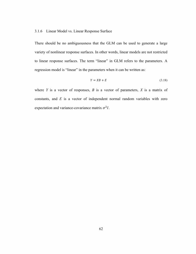
62

3.1.6 Linear Model vs. Linear Response Surface

There should be no ambiguousness that the GLM can be used to generate a large

variety of nonlinear response surfaces. In other words, linear models are not restricted

to linear response surfaces. The term “linear” in GLM refers to the parameters. A

regression model is “linear” in the parameters when it can be written as:

(3.18)

where Y is a vector of responses, B is a vector of parameters, X is a matrix of

constants, and E is a vector of independent normal random variables with zero

expectation and variance-covariance matrix .

63

3.2 Possibilistic Linear Regression

3.2.1 Background

Despite the wideness of application fields and success in many areas, linear

regression analysis is often challenged when the relationship between the response

variable and predictor variable(s) is vague, the number of observations is not

sufficient, the distribution assumption of the errors is hard to verify, etc. On the other

hand, PLR, as one of the fuzzy linear regression techniques, was introduced to

overcome some of these limitations to a certain extent. The fundamental difference

between the underlying assumptions of the two techniques is on the deviations

between the observed values and the estimated values, which are supposed to be

measurement or observation error in linear regression, but are assumed to depend on

the indefiniteness of the system structure in PLR [84]. The earliest formulation of

PLR was later named as Min problem, which minimizes the fuzziness such that the

membership of every estimated interval is above a certain threshold. Two other

formulations, Max problem [85, 86] and Conjunction problem [87] were then

proposed by Tanaka, et al. Other contributions to fuzzy regression include fuzzy least

square regression, etc. [7, 79]. Similar to linear regression analysis, fuzzy linear

regression has also been applied to various forecasting applications, such as sales

64

forecast [30] and energy forecast [80]. The conceptual differences between the two

techniques are listed in

Table 3.1 Conceptual differences between MLR and PLR

Category Multiple Linear Regression Possibilistic Linear Regression Model General Linear Models Possibilistic Linear Models System Crisp Vague Error sources Observation error Fuzziness of the system

parameters Error distribution Normal, zero mean Symmetric triangular membership Objective function Least square errors Minimize fuzziness Parameter estimation Quadratic programming Linear programming Solution Close form Feasible/infeasible Formulation extensions

Weighted least squares, etc

Max problem, Conjuction problem, etc.

Several papers offered the comparative assessment and investigation among linear

regression analysis and various fuzzy regression methods [7, 30, 79]. Heshmaty and

Kandel discussed two sales forecasting techniques [30]. One involved linear

regression analysis, which was a study of the international market sales of cameras

done by John Scott Armstrong. The other one was to use the PLR for computer and

peripheral equipment sales. Instead of comparing the two techniques, the paper was

focused more on how to build a PLM. The authors offered a detailed discussion of

Armstrong’s approach and then adopted it to the model development. In other words,

linear regression analysis was used as the base for developing the PLM. Savic and

65

Pedrycz proposed a two-step procedure for building fuzzy regression models, and

compared the results with Tanaka’s possibilistic regression analysis. The first step of

this proposed procedure was to fit the regression line to determine the center of each

parameter. Then the spread of each parameter was determined by minimizing the

fuzziness [79]. Chang and Ayyub’s paper discussed four different fuzzy regression

methods including fuzzy regression using minimum fuzziness criterion, fuzzy least

squares regression using maximum compatibility criterion and minimum fuzziness

criterion, and interval regression [7]. The aspect of least squares was emphasized in

the discussion. The comparisons were mainly devoted to the four fuzzy regression

methods, while the ordinary linear regression was used for the benchmarking

purpose.

66

3.2.2 Possibilistic Linear Models

In the PLM, deviations between the observed values and the estimated values are

assumed to depend on the indefiniteness of the system structure. These deviations are

regarded as the fuzziness of the parameters of the system rather than the observation

errors. A possibilistic linear function can be defined as:

(3.19)

where x is non-fuzzy, and is a fuzzy number. In this dissertation, we assume that

the type of fuzzy parameter is a symmetrical triangular fuzzy number with the

center denoted by α and the spread denoted by :

1 | | ,

0, (3.20)

where c 0.

As a consequence, the membership function of is obtained as the following:

1| |

, 01, 0, 00, 0, 0

(3.21)

where | | | |, … , | | , and µY y 0, when | | | | [85].

To formulate a PLM, the following are assumed[86]:

1) The data can be represented by a PLM:

(3.22)

where , … , .

67

2) The type of fuzzy parameter A is a symmetrical fuzzy number as defined in

(3.20);

3) Given the input-output relations x , y , i 1, … , N, and a threshold h, it must

hold that

, 1, … , . (3.23)

4) The index of fuzziness of the PLM is

∑ | | (3.24)

where | | is the spread of Y .

With the above assumptions, identification of the parameters of the PLM can be

formulated as a linear programming (LP) problem [26]:

Min , ∑ | | (3.25)

s.t.

| | | |

| | | |

0

1, … ,

The above formulation is an LP problem with 2(N+1) variables and 2N explicit

constraints. Concerns were raised regarding the computational difficulties of solving

this linear programming formulation [7]. In the computational experiments conducted

in this dissertation, the resources (time and computer resources) taken to estimate the

68

parameters of the PLMs through solving this LP formulation is acceptable but close

to the limit as the complexity of the model grows to certain size.

69

3.3 Artificial Neural Networks

ANN mimics human brains to learn the relationship between certain inputs and

outputs from experience. Figure 3.1 shows an example of a three-layer feed-forward

ANN, a typical ANN deployed for STLF, which is consists of an input layer, a hidden

layer, and an output layer, interconnected by some modifiable weights, represented by

the links between the layers. The computational units in each layer are called neurons.

The hidden and output neurons usually calculate their outputs as a sigmoid function

of their inputs:

(3.26)

A bias unit is connected to each neuron other than the ones in the input layer.

In Figure 3.1, the following notations are made:

• Inputs to the input neuron i: xi, i = 1, … I

• Weights from the input neuron i to the hidden neuron j: aij; Let a0j represents

the bias unit of the hidden neuron j, where j = 1, …J.

• Inputs to the hidden neuron j: uj, where

∑ (3.27)

• Outputs from the hidden neuron j: yj, where

(3.28)

70

• Weights from the hidden neuron j to the output neuron k: bjk; Let b0k

represents the bias unit of the output neuron j;

• Inputs to the output neuron k: vk, k = 1, …K.

∑ (3.29)

• Outputs of the output neuron k: zk;

(3.30)

A neural network has to be configured such that the application of a set of inputs

produces (either 'direct' or via a relaxation process) the desired set of outputs. Various

methods to set the strengths of the connections exist. One way is to set the weights

explicitly, using a priori knowledge. Another way is to 'train' the neural network by

feeding it teaching patterns and letting it change its weights according to some

learning rule. The most widely applied learning rule in STLF is supervised learning,

in which the network is trained by providing it with input (e.g., weather variables,

calendar variables, and preceding hour loads) and matching output (e.g., load).

While learning is to find the coefficients or weights (aij, bjk) that provide the best fit

between the network output (z) and target function value (t), backpropagation is one

of the simplest and most general methods for supervised training of multilayer neural

networks. Mean squared error is minimized in backpropagation:

∑ ∑ ⁄ (3.31)

71

where N is the number of examples in the data set; K is the number of outputs of the

network; tkn is the kth target output for the nth example, zkn is the kth output for the

nth example.

Figure 3.1 A three-layer feed-forward artificial neural network.

72

3.4 Diagnostic Statistics

In the literature of load forecasting, MAE and MAPE are mostly used to report the

accuracy of a forecast. To describe the distribution of the AE and APE in detail, other

than mean, the following statistics can be included: standard deviation, minimum,

25th percentile, median, 75th percentile, and maximum.

In practice, several engineering concepts (in a calendar year) are often of interest of

one or more departments for various business needs.

1) Hourly load. In a leap year, the loads of the 8784 hours are used for

calculation; otherwise, the loads of 8760 are used.

2) Hourly load of a specific hour of the day, day of the week, or month of the

year.

3) Hourly load of a specific holiday.

4) Hourly load of the surrounding days of a specific holiday. The surrounding

days may include a surrounding weekend, if the holiday falls into Monday or

Friday. They may also include the adjacent weekdays. If the holiday falls into

Monday, the Friday of the last week and the Tuesday of this week can be

considered as the adjacent weekdays.

5) Daily, monthly, or annual energy. For instance, daily energy can be calculated

by summing up the load of each hour in the day.

73

6) Daily, monthly, or annual peak load. For instance, daily peak load is the

maximum hourly load of a day.

7) Daily, monthly, or annual peak hour load. The peak hour is when the actual

peak load occurs during a day, month or year.

8) Daily, monthly, or annual valley load. For instance, daily valley load is the

minimum hourly load of a day.

9) Daily, monthly, or annual valley hour load. The valley hour is when the actual

valley load occurs during a day, month or year.

The combinations of the applicable statistics and engineering concepts mentioned

above form the performance report of a formal, published load forecast across the

organization.

In this dissertation, for the simplicity of presentation, MAPE of the hourly load of a

calendar year is used as the major diagnostic statistic. Since STLF is the focus of this

work, only hourly load related statistics are presented.

The diagnostic statistics are produced in one to all of the following four sets:

1) Take the years from 2005 to 2007 as modeling data, and 2008 as testing data,

to calculate the MAPE of the hourly load forecast in 2008.

2) Over the time span from 2001 to 2009, take three consecutive years as

modeling data, and the next year as testing data, to calculate the MAPE of this

74

testing year. Consequently, six MAPEs would be calculated for the years 2004

to 2009 respectively.

3) Take the years from 2005 to 2007 as modeling data, and the next period of

updating cycle or forecasting horizon (one hour, one day, one week, two

weeks, or a year) as testing data, to calculate the forecasted load of this testing

period. Then roll the actual data of this period to the modeling data to

recalculate the model, and forecast the next period, and so forth, until all the

hours in 2008 are forecasted. Finally, calculate the MAPE of the hourly load

forecast in 2008.

4) Over the time span from 2001 to 2009, take the three consecutive years as

modeling data, and the next period of updating cycle or forecasting horizon

(one hour, one day, one week, two weeks, or a year) as testing data, to

calculate the forecasted load of this testing period. Then roll the actual data of

this period to the modeling data to recalculate the model, and forecast the next

period, and so forth, until all the hours in the next year of the three modeling

years are forecasted. Calculate the MAPE of the hourly load forecast of this

testing year. Consequently, for each given period of updating cycle or

forecasting horizon, six MAPEs would be calculated for the years 2004 to

2009 respectively.

75

Notice that the first set is a special case of the third one by specifying the period of

updating cycle/forecasting horizon as one year. The second set is a special case of the

fourth one.

76

4 Multiple Linear Regression for Short

Term Load Forecasting

MLR analysis, as one of the earliest and widest applied techniques in the STLF field,

has been playing the role of the underdog for a long time. However, the MLR based

approaches developed in the past are not shown to fully utilize the power of this

technique, which is partially due to the limitation of the computing environment in

the old days. This chapter proposes a modern approach to apply MLR to STLF. The

use of qualitative predictor variables, polynomial regression, and interaction

regression are emphasized and demonstrated using the case study of one week ahead

hourly forecast for a medium US utility. The proposed models have been in

production use in this utility since 2009 with excellent performance.

77

4.1 Benchmark

4.1.1 Motivation

While STLF is considered as the engine of the prospective forecasting department in

our case study, benchmarking is the first step of the STLF process. A benchmark

should be able to serve as:

1) A reasonably accurate forecast. Naïve forecast, e.g., using last year’s load as

the predicted load, is not what we are looking for in the benchmarking

process. The benchmarking forecast needs to have some credibility of

catching up the salient feature of the load profiles.

2) A base case to show the improvement of the future STLF development. As a

utility keeps revising and improving the current STLF model, justifications

need to be made based on the improvement of accuracy, model complexity,

and so forth. The benchmarking model is the starting point of this entire

development.

3) A communication bridge within and outside the organization, including load

forecasters, planners, operations and planning managers, executives, the board

of directors, and commissioners, etc. A load forecast developed by the

forecasters needs to be approved by the managers. When shared with other

departments, the forecast has to be understood by and acceptable to the users.

78

When the utility is defending the rate case, there should be at least one

interpretable version of forecast presented to the regulators.

4) A platform to compare with the peer utilities. To keep the utility standing on a

competitive position in the market, the forecast can be inaccurate, but should

not be a lot worse than the competitors. When the forecast is found to be not

accurate enough, issues leading to this inaccuracy need to be identified, such

as data quality issues, weather forecasting issues, or capability of the

forecasters, etc. A commonly used benchmarking model can be beneficial to

the utility in the diagnosis process.

79

4.1.2 Evaluation criterion

With the above considerations, a benchmarking process should be evaluated from, but

not limited to, the following aspects:

1) Applicability. The process should utilize the tangible resources (both human

resources and data resources) in the utility. For instance, if the utility is not

able to get the data history of relative humidity, the benchmark model should

not include relative humidity as a predictor variable.

2) Simplicity. The benchmark should be easily interpretable. And it should not

take too much effort to produce a benchmark.

3) Reproducibility. The benchmarking process should be documentable, and the

benchmark should be reproducible based on the documentations. Namely, the

benchmark should not involve too many subjective judgments. If engineering

heuristics is involved, the parameter tuning process should be well defined.

The model and the associated documentation should be consistent.

4) Accuracy. Although accuracy is not the most important evaluation criteria for

a benchmark, the salient features of the load series should be captured during

the benchmarking process, which is expected to result in a much higher

accuracy level than a naïve forecast.

80

With the above considerations, a regression based approach is taken to produce the

benchmarking model, and then customized to become a production model for a

utility.

81

4.1.3 Benchmarking Model

The third set of diagnostic statistics with updating cycle and horizon of one hour, one

day, one week, two weeks, and one year described in Section 3.4 is used in the

development of the benchmarking model. Figure 4.1 shows the load series from 2005

to 2008, where the following observations can be obtained:

1) Figure 4.1 shows an overall increasing trend year by year. This trend may be

due to temperature increase and/or human activities. Since it is hard to draw a

conclusion from Figure 4.2 that the temperature has an increasing trend, we

can infer that human activities are the major cause of the increasing trend in

energy consumption over the years.

2) Figure 4.1 shows one peak load period in winter and the other peak load

period in summer every year, which seems to be a seasonal pattern.

Considering Figure 4.2, the winter peak load occurs during the valley

temperature period in winter, and the summer peak load occurs during the

peak temperature period in summer, which provides the evidence that the

seasonality of the temperature leads to the seasonality of the energy

consumption. Yet, it is not clear at the moment whether there is a seasonality

of human activities that affect the load in the monthly resolution.

82

3) Figure 4.1 shows that the summer peak is higher than the winter peak every

year, which tells that electricity is primarily used for cooling in the summer.

And it also tells that some electricity is used for warming in the winter.

4) Figure 4.1 shows one valley in spring and the other valley in fall every year,

which is the result of less need of air conditioning comparing with winter and

summer.

We define a quantitative variable (Trend) for the entire span of the available data

(2001 - 2009) to capture the increasing trend by assigning the natural number to each

hour in the natural order. For instance, the Trend variable of the first hour in 2001 is

1, the second hour in 2001 is 2, and so forth. It should be noticed that such a trend

only belongs to the utilities with a stable service territory and local economics. The

significant business event, such as merging two utilities or splitting one utility into

two, and recessions or booms may affect the linearly increasing trend in the system

level. Therefore, the benchmark model discussed in this dissertation is not directly

applicable to these situations.

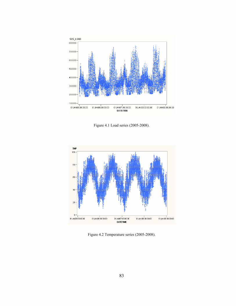
83

Figure 4.1 Load series (2005-2008).

Figure 4.2 Temperature series (2005-2008).

84

The relationship between the load and temperature has been intensively studied

during the past several decades. Figure 4.3 shows the load temperature scatter plot of

a medium utility in the US. Both piecewise linear functions and 3rd ordered

polynomials of the temperature can be applied to model the load. The piecewise

linear functions need the cut-off temperature(s), which may not be exactly the same in

different service territories. The southern part of the United States may have a

different cut-off temperature from the northern part, because the comfortable

temperature zone may be different for the people living in the different regions, or

different share of gas and electricity heaters. Therefore, the 3rd ordered polynomials

of the temperature are used to predict the load for the benchmarking purpose.

Figure 4.3 Load-temperature scatter plot (2005-2008).

85

It is well known that there are three seasonal blocks in the load series: day, week, and

year. There can be different treatments to each block depending upon the load

consumption behavior of the particular service territory. For example, the 7 days of a

week can be modeled by a qualitative variable with 2 classes (weekdays and

weekends), 3 classes (weekdays, two weekend classes), etc. In different countries, the

weekends may be defined differently. For instance, Thursday and Friday are

weekends in Iran. As a benchmark model, the qualitative variables (Hour, Day, and

Month) with 24, 7, and 12 classes, are used to model the 24 hours of a day, 7 days of

a week, and 12 months of a year respectively. Namely each seasonal block is

decomposed into the unit of the highest resolution.

Normally an afternoon is warmer than a midnight. A summer is warmer than a winter.

Figure 4.4 to Figure 4.6 show the load temperature scatter plots of 12 months and 24

hours. It can be observed that major or slight differences exist among these plots,

which implies that the model should include the interaction effects between the

polynomials of the temperature and the calendar variables Hour and Month

respectively.

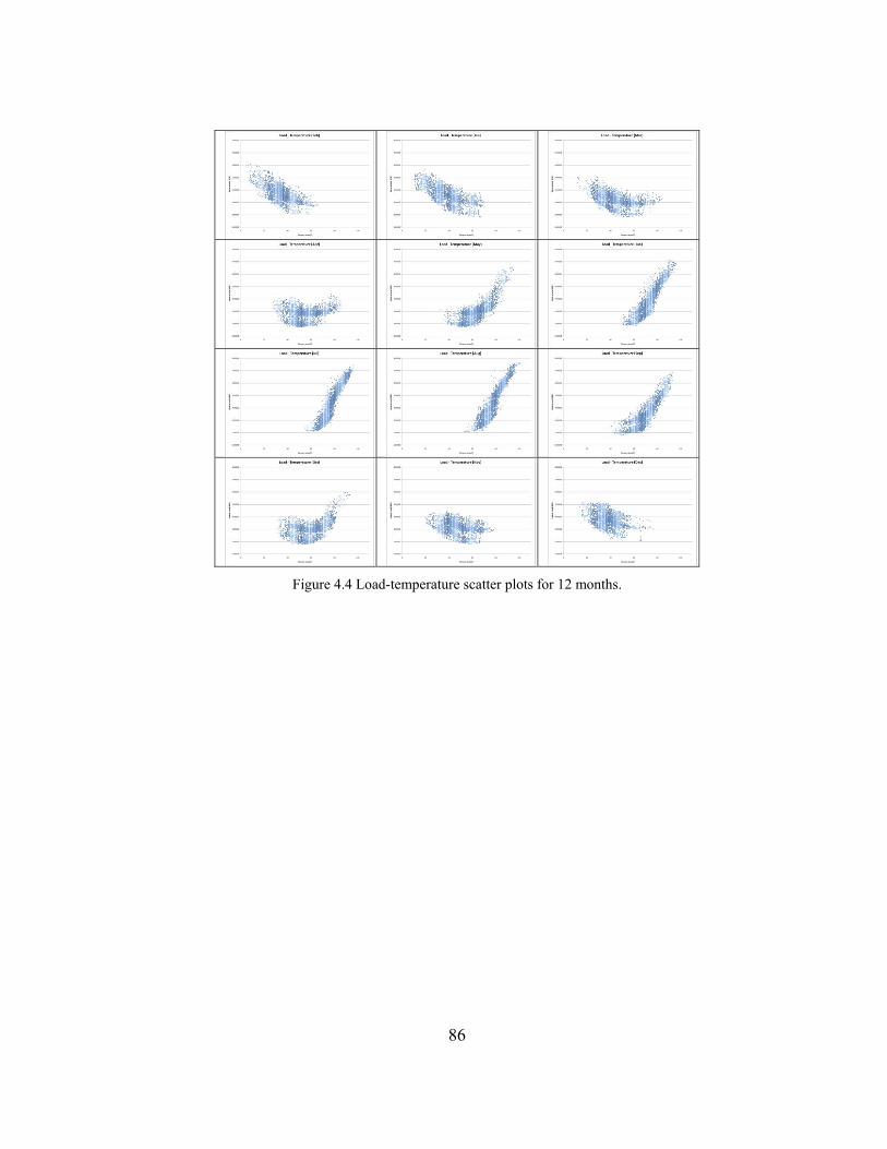
86

Figure 4.4 Load-temperature scatter plots for 12 months.

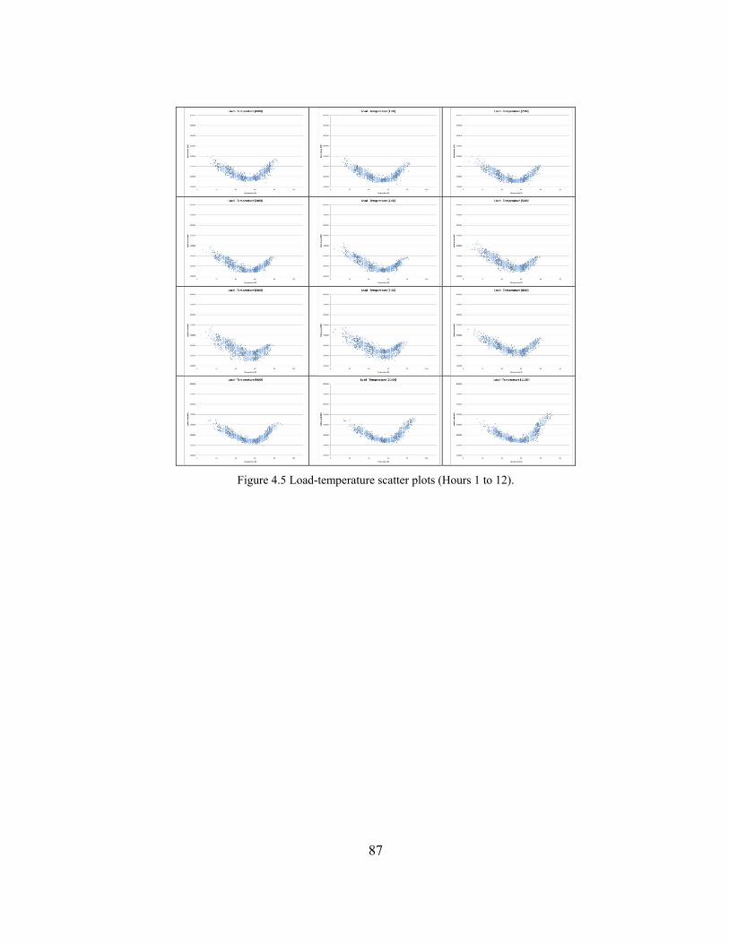
87

Figure 4.5 Load-temperature scatter plots (Hours 1 to 12).

88

Figure 4.6 Load-temperature scatter plots (Hours 13 to 24).

The hours in different days of a week may result in different load due to human

activities. For instance, there may be lower load in the morning of the weekends than

the other mornings, because people do not have to get up as early as weekdays to go

to work, which results in less load at home and office buildings in the weekend

mornings. Therefore, the interaction effect between Hour and Day should be included

in the benchmark model.

89

With the intuition and analysis above, we construct seven models as listed in Table

4.1, where the header row shows the candidate regressors in the mode. The

interaction effect is implemented by multiplication, which is denoted by “×”. “Y”

indicates that the corresponding regressor(s) is/are included in the model. When a

qualitative predictor variable interacts with a quantitative one, this quantitative term

can be taken out from the model without affecting the diagnostic statistics. Therefore,

B5 and B6 do not have to include the third order polynomials of temperature as the

main effects. When two qualitative predictor variables interact together, both terms

can be taken out from the model. Therefore, B7 does not have to include Hour or Day

as the main effects.

Table 4.1 Benchmark candidates

Trend T T2 T3

Hour Month Day Hour×T Hour×T2

Hour×T3

Month×T Month×T2

Month×T3

Day ×Hour

B1 Y Y B2 Y Y Y B3 Y Y Y Y B4 Y Y Y Y Y B5 Y Y Y Y Y B6 Y Y Y Y Y Y B7 Y Y Y Y Y

The performance of the seven candidates is listed in Table 4.2. The results show that

as the updating cycle and forecasting horizon get longer, the errors are getting larger.

90

Another observation is that the models are getting more accurate from B1 to B7.

Therefore, the benchmarking model B7, which is named as GLMLF-B (General

Linear Model based Load Forecaster - Benchmark), can be written as:

Y = β0 + β1×Trend + β2×Day×Hour + β3×Month + β4×Month×T + β5×Month×T2 +

β6×Month×T3 + β7×Hour×T + β8× Hour×T2 + β9× Hour×T3 .

(4.1)

Table 4.2 MAPEs of the seven benchmarking model candidates.

1 hour 1 day 1 week 2 weeks 1 year B1 13.60 13.60 13.62 13.63 13.68 B2 7.43 7.44 7.47 7.49 7.60 B3 6.72 6.73 6.78 6.79 6.90 B4 6.68 6.69 6.75 6.75 6.86 B5 5.85 5.86 5.92 5.92 6.03 B6 5.38 5.40 5.47 5.47 5.60 B7 4.96 4.98 5.04 5.06 5.20

91

4.2 Extensions of GLMLF-B

4.2.1 VSTLF with Preceding Hour Load

One of the underlying assumptions in GLMLF-B is that the loads in adjacent hours

are independent of each other. In practice, it is normally beneficial to the accuracy of

the short horizon, e.g., one hour ahead to one day ahead, to include the preceding

hour load in the model. Therefore, the following extension, GLMLF-L1 is proposed

for VSTLF:

Y = β0 + β1×Trend + β2×Day×Hour + β3×Month + β4×Month×TMP +

β5×Month×TMP2 + β6×Month×TMP3 + β7×Hour×TMP + β8× Hour×TMP2 + β9×

Hour×TMP3 + β10×Load(t-1)

(4.2)

where Load(t-1) represents the load of the preceding one hour.

If the forecasting horizon is more than an hour, the forecasted load, instead of actual

load is used as an input to forecast the next hour load. As the forecasting horizon gets

longer, this forecasted load becomes more and more inaccurate. Therefore, the

forecasting error may increase due to the penalty of the inaccurate information of

preceding hour load.

92

4.2.2 MTLF/LTLF with Economics

Many econometric factors, such as employment, housing stock, and so forth, can be

used to model the energy consumption and be used to drive the long term trend of the

load. This dissertation uses Gross State Product (GSP) of the local state to represent

the economy of the utility’s service territory simply to demonstrate how to extend

GLMLF-B for MTLF and LTLF. Detailed study can be conducted to come up with

some specific economical index to increase the forecast accuracy. The following

model, GLMLF-E3 is proposed, where the GSP replaces the linear trend and interacts

with all the other terms:

Y = β0 + β1×GSP + β2×Day×Hour×GSP + β3×Month×GSP + β4×Month×TMP×GSP

+ β5×Month×TMP2×GSP + β6×Month×TMP3×GSP + β7×Hour×TMP×GSP +

β8×Hour×TMP2×GSP + β9×Hour×TMP3× GSP .

(4.3)

93

4.3 Customization

The benchmarking model GLMLF-B can be applied to a generic utility, since the

knowledge of a specific utility is not involved in the development, which also means

that the model can be improved by incorporating the local information of a given

utility. This section introduces the methodology and procedure of customizing the

benchmarking model to a model for STLF.

The third set of diagnostic statistics with updating cycle and horizon of one day, one

week and two weeks described in Section 3.4 is used in the development of the

customized model. In this section, the winning models are picked by first looking at

one week ahead forecasting accuracy, then one day ahead, and then two weeks ahead.

If the models tie on all of these three measures, the one with the least complexity is

picked as the winning model.

4.3.1 Recency Effect

In psychology, recency effect refers to the principle that the most recently presented

items or experiences will most likely be remembered best. Adopting this concept to

STLF, we can infer that the most recent temperatures will most likely to be

“remembered” by the load in the next hour. In other words, the load can be affected

94

by the temperatures of the preceding hours. The following procedure is proposed to

model the recency effect of temperature:

Step 1: Add the simple moving average of the temperatures during the preceding 24

hours. The resulting model is named as RT0. The simple moving average is calculated

as following:

∑ =−=

24

124/)()(

kavg ktTtT (4.4)

If RT0 is not more accurate than GLMLF-B, use GLMLF-B for the next Step.

Step 2: Gradually add the preceding hour temperatures to RT0 with the recent ones

first, until the incremental MAPE improvement is less than 1% or the temperatures of

the preceding three hours are all added to the model. The resulting models are named

as RT1, RT2, and RT3 respectively. Pick the best one among these four models

including RT0 or GLMLF-B, and then go to Step 3.

Step 3: Replace the average temperature by the weighted moving average of the

temperatures of the preceding 24 hour period. The weighted moving average is

calculated as following:

∑∑ =−

=− −=

24

1124

11 /)()(

kk

kk

w ktTtT αα (4.5)

In this chapter, the smoothing factor α is determined by using values from 0.95 to

0.80 in decreasing steps of 0.05. The resulting models are named as RT4 to RT7

respectively. A wider range and finer resolution can be tried to fine tune the model

95

and achieve better accuracy. When α is 1, the weighted moving average is equivalent

to the simple moving average. Pick up the best model among the five candidates (four

generated in Step 3 and the winning model picked up in Step 2).

In the above procedure, the existence of any specified temperature (T) in the model

includes six interaction effects: Month×T, Month×T2, Month×T3, Hour×T, Hour×T2

and Hour×T3. In other words, adding a new temperature to the model means to add

the six corresponding interaction effects. Adding up to preceding three hours of

temperature is set as one of the stopping rules in Step 2 due to the concern of

efficiency. The more temperatures added to the model, the longer it takes for a run.

For the utilities with a powerful computer, this restriction can be alleviated.

In the case study of this utility, the performance of the seven candidate models is

shown in Table 4.3. The best model among RT0 to RT3 is RT3, which serves as the

base model of Step 3. Among the five models (RT3 to RT7), RT5 is the best one.

After evaluating all of these seven candidates, the following model with the

smoothing factor 0.90, named as GLMLF-T is considered for the further

development:

Y = β0 + β1×Trend + β2×Day×Hour + β3×Month + β4×Month×T(t) +

β5×Month×T(t)2 + β6×Month×T(t)3 + β7×Hour×T(t) + β8×Hour×T(t)2 +

β9×Hour×T(t)3 + β10×Month×T(t-1) + β11×Month×T(t-1)2 + β12×Month×T(t-1)3 +

β13×Hour×T(t-1) + β14×Hour×T(t-1)2 + β15×Hour×T(t-1)3 + β16×Month×T(t-2) +

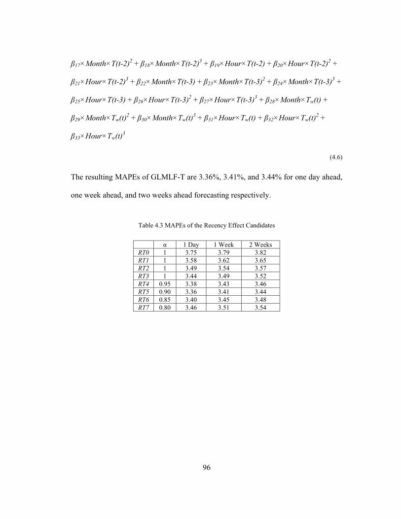
96

β17×Month×T(t-2)2 + β18×Month×T(t-2)3 + β19×Hour×T(t-2) + β20×Hour×T(t-2)2 +

β21×Hour×T(t-2)3 + β22×Month×T(t-3) + β23×Month×T(t-3)2 + β24×Month×T(t-3)3 +

β25×Hour×T(t-3) + β26×Hour×T(t-3)2 + β27×Hour×T(t-3)3 + β28×Month×Tw(t) +

β29×Month×Tw(t)2 + β30×Month×Tw(t)3 + β31×Hour×Tw(t) + β32×Hour×Tw(t)2 +

β33×Hour×Tw(t)3

(4.6)

The resulting MAPEs of GLMLF-T are 3.36%, 3.41%, and 3.44% for one day ahead,

one week ahead, and two weeks ahead forecasting respectively.

Table 4.3 MAPEs of the Recency Effect Candidates

α 1 Day 1 Week 2 Weeks RT0 1 3.75 3.79 3.82 RT1 1 3.58 3.62 3.65 RT2 1 3.49 3.54 3.57 RT3 1 3.44 3.49 3.52 RT4 0.95 3.38 3.43 3.46 RT5 0.90 3.36 3.41 3.44 RT6 0.85 3.40 3.45 3.48 RT7 0.80 3.46 3.51 3.54

97

4.3.2 Weekend Effect

During the weekends, many office buildings and factories are closed, which causes

fewer loads than those of workdays. People may get up late in the morning during

weekend, which shifts the morning peak one or two hours later than a normal work

day. The load profile of the two weekend days (Saturday and Sunday) may be

distinct. For instance, people may go to church on Sunday morning, while some

department stores open later and close earlier on Sunday.

On the other hand, People have more non-work-related activities in the weekends

than regular weekdays. These activities may start from Friday, the day before the

weekend. For instance, party time may be arranged on Friday nights, which leads to

late shower and late sleep. After a weekend, the factories need to resume the

production line, which may result in more energy consumption than usual. Therefore,

the morning of a Monday may be different from the mornings of the other weekdays.

There may as well be other local customs that result in a particular load profile of

some weekday compared to the others. Overall, the load profiles in different days of a

week may be different, which is called the weekend effect.

To customize the STLF model and incorporate the weekend effect of the utility, the

days of the week should be grouped correspondingly to reflect the local load profile.

Seven representative ways of grouping the days of a week are listed in Table 4.4, of

which most appeared in the literature. It should be noticed that the referred STLF

98

models were developed for the utilities located in different areas, or countries. For

instance, in Iran and other Islamic countries, weekend is Friday instead of Sunday for

Christian countries. Therefore, W4 also includes the grouping method in [3], which

groups Monday to Thursday together, and separates Friday, Saturday, and Sunday.

For the countries sharing the same weekend, the grouping methods may still be

different due to the different custom that results in different load consumption

behaviors. Even in the same country, e.g., US, the day type groups may still be

different, because different service territory may contain different share of customer

types, such as residential land and office buildings.

Since there are only seven days in a week, enumeration of the selected possibilities,

e.g., the seven candidates listed in Table 4.4, is feasible in the modern computing

environment. The results are listed in Table 4.4 as well. Notice that the grouping

method of W7 is the same one used in the benchmarking model as well as GLMLF-T.

The results corresponding to each grouping method are calculated by replacing the

Day variable in GLMLF-T by the ones listed in Table 4.4. Among the seven

candidates, W6 and W7 have the better forecast accuracy in all the three horizons than

the other five candidates. While W6 and W7 are tied based on the MAPEs, W6 is

selected due to the fewer degrees of freedom the grouping method brings to the model

comparing with W7. This winning model is named as GLMLF-TW.

99

Most of the grouping methods listed in Table 4.4 are either based on engineering

judgment, or based on observations from plots of hourly load curves. The hourly load

curves can be developed by either averaging the loads over a period, e.g., a calendar

year, or taking several typical days. The effectiveness of these methods can be

affected by temperature, while we can hardly find seven days of a week with exactly

the same temperature profile. In this dissertation, instead of the actual load curves, we

plot the coefficients of the interaction term Day×Hour, which are obtained from

GLMLF-T, as shown in Figure 4.7, to reinforce the decision made above for picking

up the winning model. Since the impact of the temperature to the load profile has

been modeled by the polynomials of the temperatures and the interactions between

temperatures and several calendar variables, these plotted coefficients can reflect the

normalized load profile of every hour during a week. The seven-day load profile in

Figure 4.7 indicates that Tuesday, Wednesday and Thursday are quite similar to each

other. In addition, the other four days are different from each other as well as Tuesday

to Thursday. Therefore, the grouping method W6 is likely to fit the model the best.

Since there are still some differences among Tuesday, Wednesday, and Thursday, the

grouping method W7 may also perform well. Notice that the morning of Monday is

different from the mornings of the other weekdays, while the evening of Friday is

similar to the evening of Saturday. The morning of Sunday is different from that of

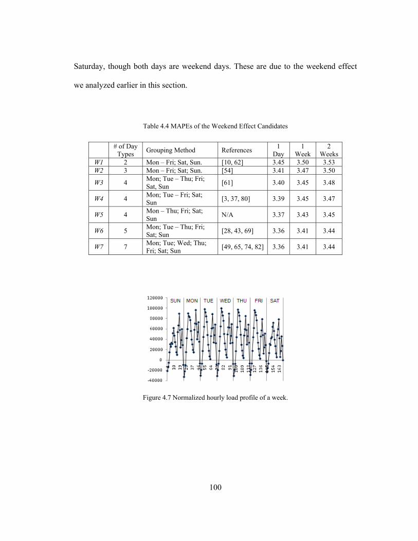
100

Saturday, though both days are weekend days. These are due to the weekend effect

we analyzed earlier in this section.

Table 4.4 MAPEs of the Weekend Effect Candidates

# of Day Types Grouping Method References 1

Day 1

Week 2

Weeks W1 2 Mon – Fri; Sat, Sun. [10, 62] 3.45 3.50 3.53 W2 3 Mon – Fri; Sat; Sun. [54] 3.41 3.47 3.50

W3 4 Mon; Tue – Thu; Fri; Sat, Sun [61] 3.40 3.45 3.48

W4 4 Mon; Tue – Fri; Sat; Sun [3, 37, 80] 3.39 3.45 3.47

W5 4 Mon – Thu; Fri; Sat; Sun N/A 3.37 3.43 3.45

W6 5 Mon; Tue – Thu; Fri; Sat; Sun [28, 43, 69] 3.36 3.41 3.44

W7 7 Mon; Tue; Wed; Thu; Fri; Sat; Sun [49, 65, 74, 82] 3.36 3.41 3.44

Figure 4.7 Normalized hourly load profile of a week.

101

4.3.3 Holiday Effect

Table 4.5 lists the public holidays for Federal employees in the US. In a calendar

year, there are six holidays falling into fixed weekdays. Among these fix-weekday

holidays, Birthday of Martin Luther King Jr., Washington’s Birthday, Memorial Day,

Labor Day, and Columbus Day are on Monday, while Thanksgiving Day is on

Thursday. On the other hand, there are four fix-date holidays: New Year’s Day,

Independence Day, Veterans Day, and Christmas Day. These fix-date holidays may

fall into any day of the week. Most Federal employees work on a Monday through

Friday schedule. For these employees, when a holiday falls on a nonworkday

(Saturday or Sunday), the holiday usually is observed on Monday (if the holiday falls

on Sunday) or Friday (if the holiday falls on Saturday).

Holiday effect on load profile is similar to weekend effect in many aspects. For

instance, a holiday, as a nonworkday for most Federal employees as well as many

other businesses, may have a different load profile from regular workdays due to

close of business, factories, and office buildings, etc. The load profiles of the holiday

surrounding days can be affected due to extended holiday activities.

The holiday effect of a specific utility is also dependent upon the local custom. For

instance, the tourist attractions city may experience more energy consumption during

the holiday seasons. Therefore, different utilities may have different holiday effects.

Holiday effect has been intensively studied in the past. Fuzzy regression was

102

proposed for holiday load forecasting in [80]. The holidays were treated as one or

several day types different than weekdays and weekends in [46, 82]. The holidays

were also treated as a weekend day. e.g., Saturday [70], Sunday [54], or Friday in Iran

[3]. The day after a holiday was treated as a Monday in [37].

Table 4.5 US Public Holidays Established by Federal Law (5 U.S.C. 603)

Date Official Name 1 Jan. 1 New Year’s Day 2 Third Monday in Jan. Birthday of Martin Luther King Jr. 3 Third Monday in Feb. Washington’s Birthday 4 Last Monday in May. Memorial Day 5 Jul. 4 Independence Day 6 First Monday in Sep. Labor Day 7 Second Monday in Oct. Columbus Day 8 Nov. 11 Veterans Day 9 Fourth Thursday in Nov. Thanksgiving Day 10 Dec. 25 Christmas Day

On the other hand, the holiday effect is more difficult to model than the weekend

effect due to, but not limit to the following:

1) There are 52 full weeks in a calendar year. Each day of the week appears at

least 52 times. However, each of the ten holidays appears once a year (New

Year’s Day may not be observed on its own calendar year if it falls on

Saturday.). Even if all of the ten holidays are treated as the same day type,

there are only ten days per year.

103

2) Although the ten holidays are the public holidays established by the Federal

government, the impacts of these holidays vary from one to another. Many

private businesses observe some of them and add other days as company

holidays. New Year's Day, Memorial Day, Independence Day, Labor Day,

Thanksgiving Day, and Christmas Day are often observed by most private

business and therefore called “big six” holidays. The variations among the

different holidays indicate that all the ten holidays should not be grouped

together. This leads to even fewer samples for modeling each holiday.

3) People’s behavior during the same holiday may vary year by year, especially

for the fix-date holidays. When a holiday falls into Monday or Friday, the

holiday and weekend together are normally called a long weekend. People

may have travel plans to make a good use of the long weekends.

Consequently, when a fix-date holiday is observed on Monday or Friday, its

impact to the load profile is different from the case when it falls on the other

weekdays.

4) The impact of the holidays to their surrounding days may not be the same for

all the holidays. For instance, the Friday after Thanksgiving Day is called

“Black Friday”, when many retail businesses open the shop in the very early

morning for big sales event. This activity would lead to higher load in the

104

morning of Black Friday than normal Friday mornings and the mornings of

the days after the other holidays.

All the above four bullets indicate that there are not many samples to model each

holiday using only the loads of the same holiday in the past years. When the amount

of training samples is small, the model would be very sensitive to the outliers. For

instance, if there is a big outage happening in the Independence Day in 2007, which is

used as the history, together with the same holiday in 2005 and 2006, to forecast the

load of 2008’s Independence Day, the result would not be accurate due to this outage.

Alternatively, the holidays can be treated as a weekend day, while the holiday

surrounding days can be treated as Monday or Friday. This is due to the similarities in

consumer behavior between the holiday effect and weekend effect. The advantage of

this approach is that dozens of weekdays and weekends are utilized to forecast the

loads of the special days including the holidays and their surrounding days. The

drawback is that the difference between the days of the week and the special days

(holidays and the surrounding days) is not fully captured. For instance, if there are

significant amount of retail businesses in the utility’s service territory, the Black

Friday morning is expected to be different from the load profile of any regular day’s

morning.

This dissertation takes the approach of modeling the special days as the regular days

of a week. Firstly the fix-weekday holidays are investigated. Then the same analogy

105

is applied to the fix-date holidays. 2005 to 2007 data are segmented into four groups:

the holidays, adjacent days before holidays, adjacent days after holidays, and the

regular days. The model GLMLF-TW is applied to the regular days, while the forecast

is performed for the other three groups with enumeration of the selected day types.

Finally, a set of empirical rules for this utility is inferred and tested through

forecasting the loads of 2008.

Three experiments are conducted to figure out whether it is the best to group the six

fix-weekday holidays as Saturdays, Sundays, or the original days of week they fall

into. The average MAPEs over the three years (2005 – 2007) of the three experiments

are listed in Table 4.6. In this dissertation, two assumptions are made for holiday

effect investigation:

1) If the maximum MAPE reduction when changing the day type of the holiday

is less than 1%, this holiday is not considered as a significant holiday.

2) If the holiday itself is not significant, its effect on the surrounding days is not

considered.

For the two significant Monday holidays, the days before are Sundays, while the days

after are Tuesdays. Since these two holidays are treated as Sundays, we would like to

investigate if treating the days before as Saturdays and the days after as Mondays can

improve the forecast accuracy. The resulting MAPEs of both approaches are listed in

106

Table 4.7, which shows that other than the day before Labor Day, alternating the day

type can improve the forecast accuracy by 0.40% to 0.45% on the surrounding days.

Thanksgiving Day is always on Thursday, while the day before is Wednesday. When

treating the day before as Wednesday, the average MAPE is 4.13%. Since

Thanksgiving Day is treated as a Saturday, an alternative day type Friday is tried to

assign to the day before. The resulting average MAPE is 4.23%, which is no better

than the original day type. Therefore, the day before Thanksgiving Day is treated as

Wednesday with no change of day type.

Since the day after Thanksgiving Day is often recognized by private business as a

company holiday, it makes sense to try more alternative day types, such as Saturday,

Sunday, Friday, and Monday, of which the average MAPEs are 2.48%, 3.37%,

2.98%, 4.55% respectively. Therefore, the day after Thanksgiving Day behaves more

like a holiday than a Friday, and it is better to treat it as a Saturday. This also explains

that Thanksgiving Day is more like a Saturday than a Sunday: the day after is more

like a nonworkday than a workday. Similarly the day after Thanksgiving Day is

treated as a Saturday but not Sunday, because the next day is Saturday (a

nonworkday).

107

Table 4.6 MAPEs of the Alternatives for the Six Fix-Weekday Holidays

Holiday Weekday (original) Saturday Sunday Birthday of MLK Jr. 3.81 3.70 3.58 Washington’s Birthday 4.55 4.76 4.33 Memorial Day 6.39 4.87 4.63 Labor Day 5.56 3.64 2.47 Columbus Day 4.06 6.82 5.64 Thanksgiving Day 8.49 5.68 7.28

Table 4.7 MAPEs of the Alternatives for the Surrounding Days of Memorial Day and Labor Day

Holiday One Day Before One Day After Sunday Saturday Tuesday Monday

Memorial Day 4.27 3.82 3.97 3.59 Labor Day 3.34 3.40 2.95 2.55

The fix-date holidays are more difficult to model than the fix-weekday ones, because

there are even less similar days for analysis. Therefore, we propose the following

strategy, which is adopted from the analogy of modeling fix-weekday holidays, to

produce the alternative day type for the fix-date holidays:

1) If a holiday is observed on Friday, treat it as Saturday, otherwise, treat it as

Sunday.

2) Justify its significance using the 1% threshold for MAPE reduction.

3) If a significant holiday is observed on Monday, Tuesday, or Wednesday, treat

the day after as Monday.

108

The results for the four fix-date holidays are listed in Table 4.8, which shows that

other than Veterans Day, the other three holidays are all significant. Using the

strategy described above, the MAPE for New Year’s Day, Independence Day, and

Christmas Day is reduced by 1.75%, 2.93%, and 1.94% respectively.

Then the results of the days after these three significant fix-date holidays are listed in

Table 4.9, which indicates that the day after Independence Day should not be changed

to the alternative day type. MAPEs of the days after New Year’s Day and Christmas

Day are reduced when applying the alternative day types.

Table 4.8 MAPEs of the Alternatives for the Four Fix-Date Holidays

Holiday Original Alternative New Year’s Day 6.42 4.67 Independence Day 6.31 3.38 Veterans Day 3.78 3.90 Christmas Day 5.91 3.97

Table 4.9 MAPEs of the Days After the Three Significant Fix-Date Holidays

Holiday Original Alternative New Year’s Day 4.11 3.51 Independence Day 3.84 3.86 Christmas Day 4.60 4.57

To sum up, the following guideline is proposed to model the special days for this

utility:

109

1) Memorial Day and Labor Day are treated as Sunday.

2) The day before Memorial Day is treated as Saturday.

3) The days after Memorial Day and Labor Day are treated as Monday.

4) Thanksgiving Day and the day after are treated as Saturday.

5) New Year’s Day, Independence Day, and Christmas Day are treated as

Sunday when they are not observed on Friday, otherwise, treat them as

Saturday.

6) The days after New Year’s Day and Christmas Day are treated as Monday

when the corresponding holiday is observed on Monday, Tuesday or

Wednesday.

The above guideline is applied to forecast 2008 load, while the updated model is

named as GLMLF-HT, and the resulting MAPEs are listed in Table 4.10. The

reduction of MAPE for all days is 0.03%, 0.03%, and 0.04% for 1 day, 1 week, and 2

weeks ahead forecast respectively comparing with the result of GLMLF-TW.

Table 4.10 GLMLF-HT vs. GLMLF-TW

Model 1 Day 1 Week 2 Weeks

All Days GLMLF-HT 3.32 3.37 3.40 GLMLF-TW 3.36 3.41 3.44

Holidays GLMLF-HT 4.46 4.49 4.50 GLMLF-TW 5.66 5.68 5.68

Surrounding Days GLMLF-HT 3.96 4.00 4.03 GLMLF-TW 3.99 4.04 4.06

Regular Days GLMLF-HT 3.25 3.30 3.33 GLMLF-TW 3.25 3.31 3.34

110

4.3.4 Exponentially Weighted Least Squares

A power system is a time-varying system, while human’s energy consumption

behavior varies over time as well. To emphasize the recent status of the system,

higher weights should be assigned to the recent observations than the older ones.

Consequently, an exponentially weighted least square approach can be deployed. The

unit weight is assigned to the earliest hour in the history. The nth hour in the history

has the weight λn-1, where the weighting factor λ≥1. When λ=1, the process becomes

ordinary least squares approach.

In this chapter, the weighting factor λ is varied from 1.00005 to 1.00020 in steps of

0.00005. The results are listed in Table 4.11. Following the rule introduced in Section

3.4, WLS3 is picked as the winning model, named as GLMSTLF-HT.

Table 4.11 MAPEs of the Exponentially Weighted Least Squares Candidates

Λ 1 Day 1 Week 2 Weeks WLS1 1.00005 3.17 3.24 3.28 WLS2 1.00010 3.08 3.17 3.22 WLS3 1.00015 3.06 3.17 3.23 WLS4 1.00020 3.06 3.20 3.28

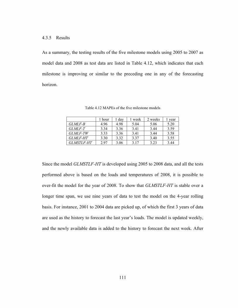
111

4.3.5 Results

As a summary, the testing results of the five milestone models using 2005 to 2007 as

model data and 2008 as test data are listed in Table 4.12, which indicates that each

milestone is improving or similar to the preceding one in any of the forecasting

horizon.

Table 4.12 MAPEs of the five milestone models

1 hour 1 day 1 week 2 weeks 1 year GLMLF-B 4.96 4.98 5.04 5.06 5.20 GLMLF-T 3.34 3.36 3.41 3.44 3.59 GLMLF-TW 3.33 3.36 3.41 3.44 3.58 GLMLF-HT 3.30 3.32 3.37 3.40 3.55 GLMSTLF-HT 2.97 3.06 3.17 3.23 3.44

Since the model GLMSTLF-HT is developed using 2005 to 2008 data, and all the tests

performed above is based on the loads and temperatures of 2008, it is possible to

over-fit the model for the year of 2008. To show that GLMSTLF-HT is stable over a

longer time span, we use nine years of data to test the model on the 4-year rolling

basis. For instance, 2001 to 2004 data are picked up, of which the first 3 years of data

are used as the history to forecast the last year’s loads. The model is updated weekly,

and the newly available data is added to the history to forecast the next week. After

112

the entire year of 2004 is forecasted, MAPEs for 2004 forecast are calculated. Then

the tests are repeated for 2002 to 2005 data, and so forth.

Table 4.13 lists the MAPEs of all the five milestones over the six forecasted years.

The various models perform differently in different years. For instance, the MAPE of

GLMSTLF-HT can be as low as 3.14% in 2006, or as high as 3.58% in 2004.

Nevertheless, it is shown that each milestone is an improvement over the preceding

one in any of the six years. The average one week ahead forecasting MAPE over six

years for GLMSTLF-HT is 3.36%, which is 36.4% better in relative error than the

benchmarking model, GLMLF-B.

Another comparison is made to show the effectiveness of modeling holiday effect.

The MAPEs of the holidays, surrounding days, and regular days forecasted by

GLMSTLF-HT are listed in Table 4.14. Over the nine years period, of which six are

used for forecasting, the average MAPE of the holidays is 4.00%, that of the

surrounding days is 3.76%, and that of the regular days is 3.32%.

Table 4.13 One Week Ahead Forecasting Performance for All Milestones

2004 2005 2006 2007 2008 2009 Avg. GLMLF-B 5.83 5.58 4.97 5.08 5.04 5.15 5.28 GLMLF-T 4.19 4.12 3.44 3.82 3.41 3.59 3.76 GLMLF-TW 4.19 4.11 3.44 3.82 3.41 3.59 3.76 GLMLF-HT 4.15 4.08 3.41 3.78 3.37 3.57 3.72 GLMSTLF-HT 3.58 3.48 3.14 3.61 3.17 3.21 3.36

113

Table 4.14 Effectiveness of Holiday Effect Modeling of GLMSTLF-HT

2004 2005 2006 2007 2008 2009 Avg. Regular Days 3.55 3.46 3.09 3.57 3.12 3.13 3.32 Holidays 3.56 3.89 4.17 4.19 4.23 3.93 4.00 Surrounding Days 3.96 3.56 3.53 4.03 3.43 4.03 3.76

Depending upon the various business needs of the STLF, the utilities may use

different engineering concepts to evaluate the forecasting performance. The following

are some typical ones used in practice:

1) Annual peak day load: the hourly load of the day when annual peak (highest

load over a year) occurs.

2) Daily peak/valley load: the highest/lowest load occurs during a calendar day.

3) Daily peak/valley hour load: the load of the hour when the daily peak/valley

load occurs.

4) Daily energy: sum of the hourly loads over a calendar day.

The MAPEs of the above concepts are listed in Table 4.15, which indicates that the

forecasting errors of the above engineering concepts are consistently low over a long

time span. In particular, the actual and predicted load profiles of the 2009 annual peak

day are plotted in Figure 4.8, where the solid line is the actual one, and the dashed

line is the predicted one. The vertical axis represents the load in kW. The horizontal

axis represents the hour of a day, starting from 12am (the 1st hour) to 11pm (the 24th

hour). The annual peak of 2009 is around 800 MW, while the MAPE of this annual

114

peak day is 2.80%. It is noticeable from Figure 4.8 that from 8am (the 9th hour) to

6pm (the 19th hour), the predicted loads are consistently higher than the actual one.

During the next few hours, the predicted loads are consistently lower. In fact this is

mainly due to the load control activity the utility performed during this annual peak

day. When the load control is active, the system load level is lower than the

hypothetically non-controlled load. After load control is off, the load would be picked

up and higher than usual for a few hours. Therefore, the daily peak can be reduced

and the energy consumption is leveraged to the couple of hours after the load control

period.

To sum up, in order to develop a GLM for STLF, the following procedure is

proposed: firstly develop a base model GLMLF-B. And then model the recency

effect, weekend and holiday effect as introduced in this chapter. Finally fine tune the

model using the exponentially weighted least squares method. A sanity check can be

performed over a longer time span if the data is available. The model developed in

this chapter is mainly for one week ahead forecasting. Therefore, the criteria to pick

up the winning models are targeting more to the accuracy of one week ahead. When

other forecasting horizon is more important, the winning model can be determined by

the alternative criteria. During production use, the above procedure can be conducted

once a year to calibrate the modeling of the various effects.

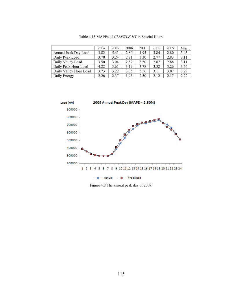
115

Table 4.15 MAPEs of GLMSTLF-HT in Special Hours

2004 2005 2006 2007 2008 2009 Avg. Annual Peak Day Load 3.82 5.41 2.80 1.95 3.84 2.80 3.43 Daily Peak Load 3.70 3.24 2.81 3.30 2.77 2.83 3.11 Daily Valley Load 3.50 3.04 2.87 3.50 2.87 2.88 3.11 Daily Peak Hour Load 4.22 3.61 3.19 3.78 3.32 3.26 3.56 Daily Valley Hour Load 3.73 3.22 3.05 3.56 3.11 3.07 3.29 Daily Energy 2.26 2.37 1.93 2.50 2.12 2.17 2.22

Figure 4.8 The annual peak day of 2009.

116

4.4 Impact of Demand Side Management to Load Forecasting Accuracy

Some utilities, including the utility for which we perform the study in this

dissertation, keep a good record of the historical load control hours. Table 4.16 briefly

shows some statistics of the DSM activities performed in this utility from 2001 to

2008. DSM hours mean the hours with load control active. DSM related hours

include DSM hours and two hours after each DSM period. DSM days mean the days

with load control active during some (or all) of the 24 hours.

Table 4.16 DSM activities (2001 – 2008)

Hours (total) DSM hours Days (total) DSM days 2001 8760 407 365 75 2002 8760 483 365 83 2003 8760 432 365 91 2004 8784 431 366 89 2005 8760 454 365 84 2006 8760 424 365 84 2007 8760 419 365 84 2008 8784 377 366 76

In this section, we examine how the forecasting accuracy would change by taking out

the DSM related hours from the modeling data, which is called preprocessed data.

Table 4.17 listed the MAPE of the five milestone models when using the

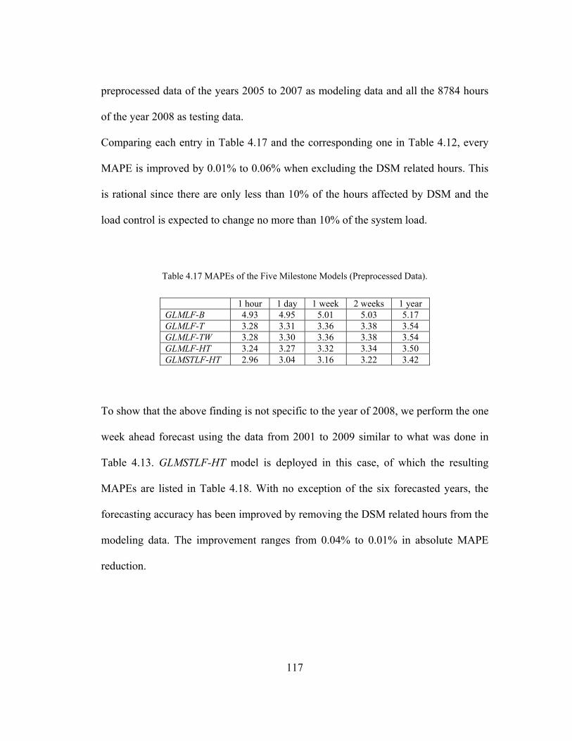
117

preprocessed data of the years 2005 to 2007 as modeling data and all the 8784 hours

of the year 2008 as testing data.

Comparing each entry in Table 4.17 and the corresponding one in Table 4.12, every

MAPE is improved by 0.01% to 0.06% when excluding the DSM related hours. This

is rational since there are only less than 10% of the hours affected by DSM and the

load control is expected to change no more than 10% of the system load.

Table 4.17 MAPEs of the Five Milestone Models (Preprocessed Data).

1 hour 1 day 1 week 2 weeks 1 year GLMLF-B 4.93 4.95 5.01 5.03 5.17 GLMLF-T 3.28 3.31 3.36 3.38 3.54 GLMLF-TW 3.28 3.30 3.36 3.38 3.54 GLMLF-HT 3.24 3.27 3.32 3.34 3.50 GLMSTLF-HT 2.96 3.04 3.16 3.22 3.42

To show that the above finding is not specific to the year of 2008, we perform the one

week ahead forecast using the data from 2001 to 2009 similar to what was done in

Table 4.13. GLMSTLF-HT model is deployed in this case, of which the resulting

MAPEs are listed in Table 4.18. With no exception of the six forecasted years, the

forecasting accuracy has been improved by removing the DSM related hours from the

modeling data. The improvement ranges from 0.04% to 0.01% in absolute MAPE

reduction.

118

Table 4.18 One Week Ahead Forecasting Performance Comparison (GLMSTLF-HT)

2004 2005 2006 2007 2008 2009 Avg. All data 3.58 3.48 3.14 3.61 3.17 3.21 3.36 Preprocessed 3.53 3.44 3.13 3.60 3.16 3.19 3.34

119

5 Possibilistic Linear Model Based

Load Forecasters

Although PLR has been applied to STLF during the past decade, the published PLMs

are not shown to be fully utilizing interactions as discussed in Chapter 4. In other

words, the underlying GLM of the PLM is not yet up to the level introduced in this

dissertation. Moreover, there is not much research devoted to studying the

relationship between the PLM and its underlying GLM in STLF. Following the

discussion in Chapter 4, this chapter compares the PLM with its underlying GLM,

and interprets the results through some numerical examples.

120

5.1 Benchmarking Model

In this section, we start with the preliminary GLMs introduced in Table 4.1 to build

the PLMs. In this chapter, all the hours from 2005 to 2007 are used for modeling,

while the year of 2008 is used for testing. The resulting MAPE of each PLM is listed

in Table 5.1 with that of the corresponding GLM for comparison purpose.

Table 5.1 MAPEs of the seven PLM based benchmarking model candidates.

PLM GLM B1 24.54 13.68 B2 14.42 7.60 B3 11.31 6.90 B4 11.51 6.86 B5 8.91 6.03 B6 8.16 5.60 B7 7.56 5.20

The results in Table 5.1 indicate the following:

1) In the specific case study we are performing, the PLM is much less accurate

than its underlying GLM.

2) As the GLM becomes more accurate, the corresponding PLM becomes more

accurate as well. The only exception is B4.

3) As the models built based on both approaches become more accurate, the

difference between the two gets smaller. The only exception is B4.

121

The last model B7 is picked as the benchmarking model of PLM and named as

PLMLF-B (Possibilistic Linear Model based Load Forecaster - Benchmark).

122

5.2 Impact of Demand Side Management to Forecasting Accuracy

As concluded in Section 4.4, the forecasting accuracy of GLMLFs can be improved

by removing DSM related hours from the modeling data. In this section, the impact of

DSM to the forecasting accuracy of PLMLFs is also investigated. We used the seven

models in Table 4.1 and the model with holiday effect and recency effect, which is

named as PLMLF-HT. The resulting MAPEs are listed in Table 5.2 together with the

results of the underlying GLMs. The following can be observed:

1) In the specific case study we are performing, the PLM is much less accurate

than its underlying GLM when the DSM related hours are excluded from the

modeling data.

2) As the GLM becomes more accurate, the corresponding PLM becomes more

accurate as well when the DSM related hours are excluded from the modeling

data.

3) As the models built based on both approaches become more accurate, the

difference between the two gets smaller.

4) Removing the DSM related hours from the modeling data helps improve the

forecasting accuracy of PLM. The only exception is B3.

5) The improvement to PLM is more significant, from the perspectives of both

relative and absolute reduction of MAPE, than that of GLM. The only

exception is B3.

123

The first three observations are consistent with the ones summarized in Section 5.1.

The reason for observation 5) is likely due to the fact that PLM is more sensitive to

the outliers than GLM. Since the DSM related hours are abnormal and most of them

can be taken as outliers, PLM gets more benefits than GLM.

Table 5.2 MAPEs of the seven PLM based benchmarking model candidates (preprocessed data).

PLM GLM B1 22.82 13.55 B2 13.62 7.54 B3 11.32 6.81 B4 11.20 6.77 B5 8.66 5.96 B6 7.74 5.57

LF-B 7.11 5.17 LF-HT 4.14 3.50

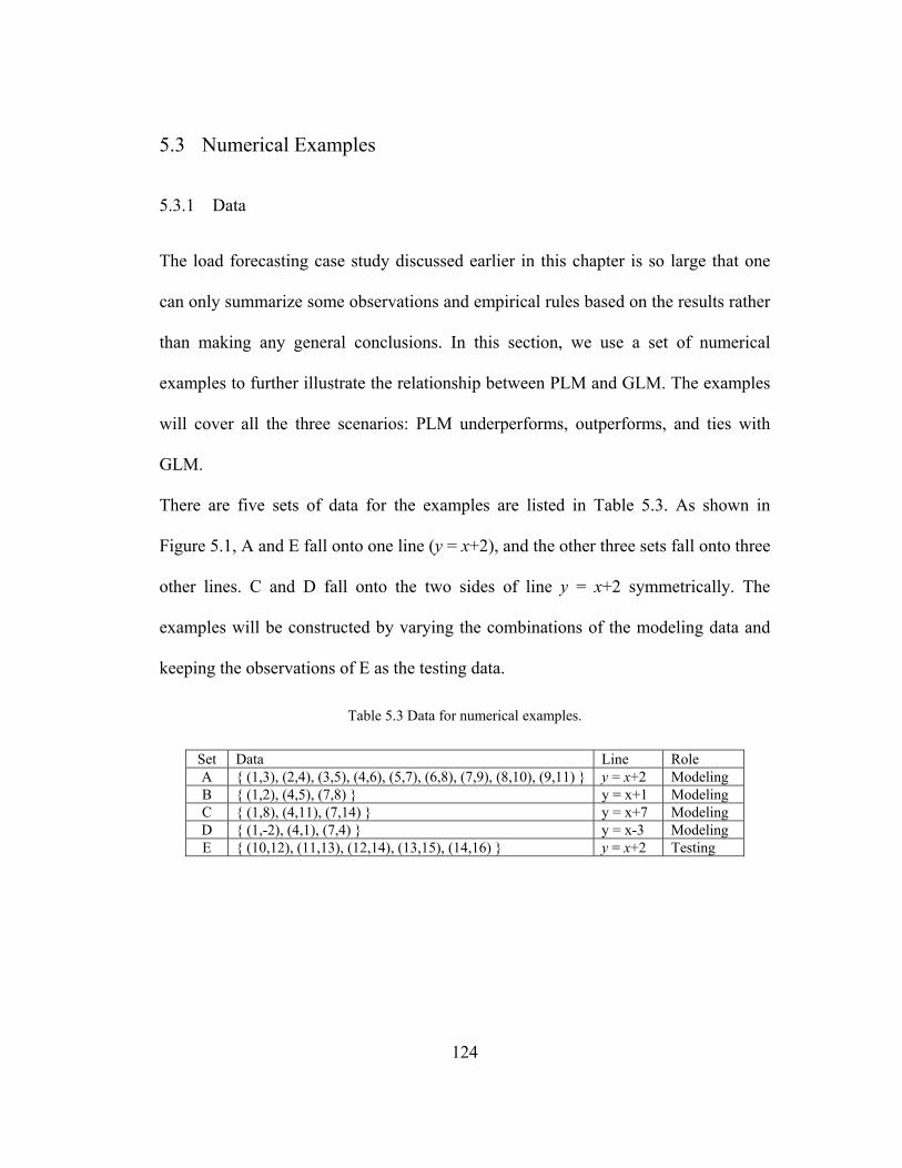
124

5.3 Numerical Examples

5.3.1 Data

The load forecasting case study discussed earlier in this chapter is so large that one

can only summarize some observations and empirical rules based on the results rather

than making any general conclusions. In this section, we use a set of numerical

examples to further illustrate the relationship between PLM and GLM. The examples

will cover all the three scenarios: PLM underperforms, outperforms, and ties with

GLM.

There are five sets of data for the examples are listed in Table 5.3. As shown in

Figure 5.1, A and E fall onto one line (y = x+2), and the other three sets fall onto three

other lines. C and D fall onto the two sides of line y = x+2 symmetrically. The

examples will be constructed by varying the combinations of the modeling data and

keeping the observations of E as the testing data.

Table 5.3 Data for numerical examples.

Set Data Line Role A { (1,3), (2,4), (3,5), (4,6), (5,7), (6,8), (7,9), (8,10), (9,11) } y = x+2 Modeling B { (1,2), (4,5), (7,8) } y = x+1 Modeling C { (1,8), (4,11), (7,14) } y = x+7 Modeling D { (1,-2), (4,1), (7,4) } y = x-3 Modeling E { (10,12), (11,13), (12,14), (13,15), (14,16) } y = x+2 Testing

125

Figure 5.1 Data for the numerical examples.

y = x + 2

y = x + 1

y = x + 7

y = x ‐ 3

‐5

0

5

10

15

20

25

1 2 3 4 5 6 7 8 9 10 11 12 13 14

A

B

C

D

E

126

5.3.2 PLM Underperforms GLM

The fuzzy parameters of the system is assumed to be symmetric triangular in the PLR

discussed in this chapter, while normal distribution is assumed to be the error

distribution for MLR. Therefore, when the boundary of the observations does not fall

symmetrically aside the nominal center, PLM would not perform well. As shown in

Figure 5.2, where the data sets A, B, and C are combined as modeling data, the upper

boundary of the observations consists of B, while the lower boundary consists of C.

The data set E is deployed as the testing data. The center of B and C is the line y = x +

3.5. The MAPE of this model is 10.83%. Observations in A are not involved in the

calculation of the PLM. On the other hand, all the observations in A, B, and C are

involved when performing MLR. The calculated GLM is y = 0.93x + 3.13. The

MAPE of this model is 2.17%. GLM outperforms PLM in this case, because the

observations in A compensate the “outliers” in B and C to a certain extent.

127

Figure 5.2 Example 1: PLM underperforms GLM.

Even if the observations in A are involved in the calculation of PLM, PLM may still

underperforms GLM. Figure 5.3 offers an example, where data sets A, B, and D are

used as modeling data. The upper boundary of the observations consists of A, while

the lower boundary consists of D. The center of B and C is the line y = x - 0.5, and the

MAPE of this model is 18.04%. On the other hand, the calculated GLM is y = 1.11x +

0.30, of which the MAPE is 2.86%. In this case, the lower boundary is so low that the

PLM is still not as good as the GLM. However, if there is a large number of

observations, e.g., double the size of data set A, falling onto the line y = x -3, the

calculated GLM can be worse than the PLM.

y = 0.93x + 3.13

y = x + 3.5

0

2

4

6

8

10

12

14

16

18

20

0 5 10 15

A

B

C

E

GLM

PLM

Linear (GLM)

Linear (PLM)

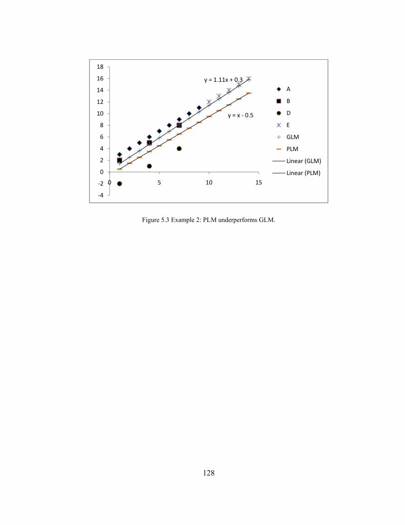
128

Figure 5.3 Example 2: PLM underperforms GLM.

y = 1.11x + 0.3

y = x ‐ 0.5

‐4

‐2

0

2

4

6

8

10

12

14

16

18

0 5 10 15

A

B

D

E

GLM

PLM

Linear (GLM)

Linear (PLM)

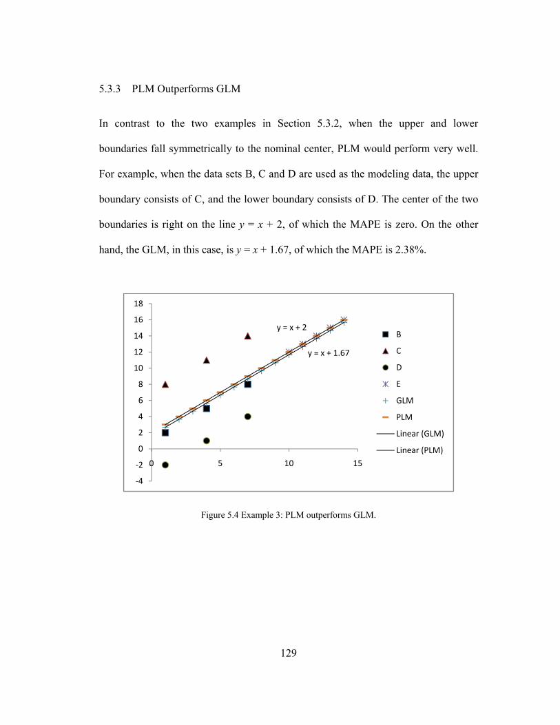
129

5.3.3 PLM Outperforms GLM

In contrast to the two examples in Section 5.3.2, when the upper and lower

boundaries fall symmetrically to the nominal center, PLM would perform very well.

For example, when the data sets B, C and D are used as the modeling data, the upper

boundary consists of C, and the lower boundary consists of D. The center of the two

boundaries is right on the line y = x + 2, of which the MAPE is zero. On the other

hand, the GLM, in this case, is y = x + 1.67, of which the MAPE is 2.38%.

Figure 5.4 Example 3: PLM outperforms GLM.

y = x + 1.67

y = x + 2

‐4

‐2

0

2

4

6

8

10

12

14

16

18

0 5 10 15

B

C

D

E

GLM

PLM

Linear (GLM)

Linear (PLM)

130

As more data close to the nominal center are added to the modeling data, GLM can be

improved. For instance, as shown in Figure 5.5, if the data set A is added, the GLM

becomes y = 1.01x + 1.78, of which is MAPE is 0.73%. Since none of the added data

contributes to the boundary, the PLM stays the same.

Figure 5.5 Example 4: PLM outperforms GLM.

y = 1.01x + 1.78

y = x + 2

‐4

‐2

0

2

4

6

8

10

12

14

16

18

0 5 10 15

A

B

C

D

E

GLM

PLM

Linear (GLM)

Linear (PLM)

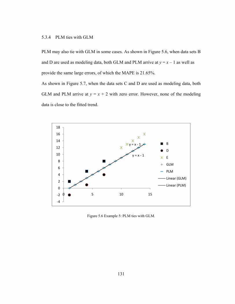
131

5.3.4 PLM ties with GLM

PLM may also tie with GLM in some cases. As shown in Figure 5.6, when data sets B

and D are used as modeling data, both GLM and PLM arrive at y = x – 1 as well as

provide the same large errors, of which the MAPE is 21.65%.

As shown in Figure 5.7, when the data sets C and D are used as modeling data, both

GLM and PLM arrive at y = x + 2 with zero error. However, none of the modeling

data is close to the fitted trend.

Figure 5.6 Example 5: PLM ties with GLM.

y = x ‐ 1

y = x ‐ 1

‐4

‐2

0

2

4

6

8

10

12

14

16

18

0 5 10 15

B

D

E

GLM

PLM

Linear (GLM)

Linear (PLM)

132


Figure 5.8 shows an extreme case: when A is used as training data, both GLM and

PLM arrive at the same model and zero MAPE. Moreover, all of the training data fall

right onto the fitted trend. This example indicates that when the system is 100%

certain with minimal observation errors, and all of the salient features are fully

captured, the corresponding PLM and GLM should be quite similar with minimal

error. A summary of the results including the models and MAPEs are listed in Table

5.4.

y = x + 2

y = x + 2

‐4

‐2

0

2

4

6

8

10

12

14

16

18

0 5 10 15

C

D

E

GLM

PLM

Linear (GLM)

Linear (PLM)

133


Table 5.4 Seven numerical examples.

Example Training Data

GLM PLM Model MAPE Model MAPE

1 A, B, C y = 0.93x + 3.13 2.17 y = x + 3.5 10.83 2 A, B, D y = 1.11x + 0.30 2.86 y = x - 0.5 18.04 3 B, C, D y = x + 1.67 2.38 y = x + 2 0 4 A, B, C, D y = 1.01x + 1.78 0.73 y = x + 2 0 5 B, D y = x - 1 21.65 y = x - 1 21.65 6 C, D y = x + 2 0 y = x + 2 0 7 A y = x + 2 0 y = x + 2 0

y = x + 2

y = x + 2

0

2

4

6

8

10

12

14

16

18

0 5 10 15

A

E

GLM

PLM

Linear (GLM)

Linear (PLM)

134

5.4 Summary and Discussion

Although lots of real-world systems are vague, the vagueness information may not be

available. Non-fuzzy data analysis is still widely applicable. It is shown in this

Chapter that PLR has no significant advantage over ordinary linear regression in the

presented load forecasting case study. Nevertheless, PLM provides an alternative to

GLM when analyzing the non-fuzzy data. The major difference between the two

approaches is on the assumption of error distribution. Linear regression analysis

assumes the errors are due to “observation errors” which are independent and

normally distributed. Therefore, the least-squares method can be employed to identify

the expected response function. PLR assumes the errors are due to the fuzziness of

the system and follow some possibilistic distribution. Under certain conditions, a

linear programming formulation can be employed to solve for the parameters of the

PLM.

With the load forecasting test cases and the numerical examples, the following can be

summarized

1) In all of the load forecasting test cases presented in this section, GLMs

outperform PLMs.

2) The PLM gets more accurate as the underlying GLM gets more accurate.

Therefore, it is recommended to keep improving the underlying GLM during

the development of the PLM.

135

3) The more advanced domain knowledge realized by the GLMs and PLMs, the

closer the forecast accuracy of the two approaches would be.

4) As shown in Example 7 of Section 5.3.4, when a crisp system is fully

understood with minimal observation error, the corresponding GLM and PLM

should be quite similar or even the same.

5) GLM is less sensitive to the outliers than PLM.

6) Depending upon the distribution of the errors, there are possibilities for GLM

to tie with, outperform, and underperform PLM.

To better utilize the capability of PLR, developing the vagueness information is a key

direction for the future work. For instance, in STLF, the load is vague when load

management is performed. The information, such as how much load was reduced

during the load management, would be beneficial to the accuracy of STLF.

136

6 Artificial Neural Networks Based

Load Forecasters

ANN has been applied to STLF for two decades with varying degree of success.

Hippert, et al. offered a high-level methodology to develop ANN models for STLF in

their review paper [31]. However, most research papers and reports just presented the

final design of the model rather than introducing the steps or summarizing the

procedure to reach the model, which makes the reproduction of the former research

work quite challenging. On the other hand, since those ANNs were developed for the

specific utilities, it is not quite meaningful for comparison purposes in our case study

even if the model can be reproduced. In this chapter, we build several typical ANNs

to compare the performance with the GLMLFs developed in Chapter 4.

137

6.1 Single Model Forecasting

Designing a three-layer feedforward ANN model for STLF involves several major

steps:

1) Determine the number of outputs: An ANN model may have only one output,

which can be corresponding to the load of one hour, or several outputs, which

can represent a 24-hour load profile if there are 24 outputs. Some drawbacks

of the multiple outputs ANN were discussed in [31]. In this chapter, we build

single-output ANN models, of which the output is load. We also try the

approach of forecasting the loads using multiple single-output models, e.g.,

the 24-hour load profile is forecasted by 24 ANNs in parallel, which is a

popular way of building ANNs for STLF.

2) Determine the number of inputs: The inputs may include weather variables,

calendar variables, and the load of the preceding hours. In this chapter, we

exclude the preceding hour loads from the inputs to the neural networks, and

compare the performance of ANN with that of GLMLFs, which do not

include the preceding hour loads either.

3) Determine the number of hidden neurons: There is no common rule for

determining the number of hidden neurons. In this chapter, we use a trial-and-

error approach: enumerating the number within a reasonable range when using

138

2005 to 2007 data for modeling and 2008 data for testing, and then pick the

best one to test on a rolling basis using 2001 to 2009 data.

In this section, we build three single-model ANN based load forecasters (ANNLFs).

The first one using only two input variables: linear trend and temperature. This model

is comparable to B1 in Table 4.1. We enumerate the number of hidden neurons from

1 to 10 by unit steps. The resulting MAPEs are listed in Table 6.1, which indicates

that 2 hidden neurons offer the most accurate results. This model is named as

ANNLF-S., while its MAPE for 2008 is 13.39%.

Table 6.1 MAPEs of ANNLF-S.

S Number of hidden neurons MAPE 1 1 15.68 2 2 13.39 3 3 15.68 4 4 18.41 5 5 18.95 6 6 16.02 7 7 16.03 8 8 13.47 9 9 14.70

10 10 14.93

In addition to the linear trend and temperature, the calendar variables, hour, weekday,

and month are added to the inputs as class variables to construct the second model,

which is comparable to GLMLF-B. We enumerate the number of hidden neurons

139

from 10 to 55 in steps of 5. The resulting MAPEs are listed in Table 6.2, which

indicates that the ANN with 40 hidden neurons is the best. This model is named as

ANNLF-BS, of which the 2008 MAPE is 5.00%.

The third model, comparable to GLMLF-HT, includes the temperatures of the

preceding three hours, the weighted temperature of the preceding 24 hours, Hour, 5-

day-type code (holiday code), and Month in addition to the linear trend and the

current hour temperature. We enumerate the number of hidden neurons from 20 to 65

in steps of 5, while the best one turns out to be 55 with the MAPE of 4.32%, as shown

in Table 6.3. This model is named as ANNLF-HTS.

Table 6.2 MAPEs of ANNLF-BS.

BS Number of hidden neurons MAPE 1 10 6.37 2 15 5.82 3 20 5.74 4 25 5.29 5 30 5.29 6 35 5.50 7 40 5.00 8 45 5.91 9 50 5.56

10 55 6.19

140

Table 6.3 MAPEs of ANNLF-HTS.

HTS Number of hidden neurons MAPE 1 20 5.41 2 25 5.29 3 30 5.05 4 35 5.18 5 40 4.78 6 45 5.24 7 50 4.58 8 55 4.32 9 60 4.46

10 65 4.53

141

6.2 Multi-model Forecasting

As the input information grows, the single-model ANNLF gets more and more

accurate. In this section, we decompose the single-model ANNLFs and forecast the

loads using multiple ANN models in parallel. As discussed in [31], the advantage of

this method is that the individual networks are relatively small, and so they are not

likely to be overfitted.

We first decompose the ANNLF-BS by hour, week, and month, such that there are 24,

7, and 12 sub-models in each case. The number of hidden neurons is enumerated from

5 to 50 in steps of 5. The resulting MAPEs are listed in Table 6.4, where the best one

of each case is highlighted in bold. These models are named as ANNLF-BM series.

Table 6.4 MAPEs of ANNLF-BM.

BM Number of hidden neurons Hour Week Month 1 5 13.49 15.32 13.45 2 10 8.81 7.46 10.51 3 15 11.06 6.45 12.07 4 20 8.30 6.61 7.19 5 25 6.52 6.39 7.71 6 30 7.32 6.97 7.41 7 35 6.68 6.80 7.12 8 40 6.91 7.29 7.47 9 45 6.58 6.92 7.31

10 50 6.91 6.49 8.23

142

We then decompose the ANNLF-HTS by hour, holiday code, and month, such that

there are 24, 5, and 12 sub-models in each case. The number of hidden neurons is

enumerated from 5 to 50 in steps of 5. The resulting MAPEs are listed in Table 6.5,

where the best one of each case is highlighted in bold. These models are named as

ANNLF-HTM series.

Table 6.5 MAPEs of ANNLF-HTM.

HTM Number of hidden neurons Hour Holiday Month 1 5 9.92 13.45 7.42 2 10 7.44 6.21 5.13 3 15 6.51 4.16 5.01 4 20 6.87 6.88 5.12 5 25 4.97 4.43 5.47 6 30 5.03 5.39 5.10 7 35 5.06 5.20 5.34 8 40 5.40 5.75 5.19 9 45 4.46 5.31 5.46

10 50 4.70 5.15 5.12

143

6.3 Comparison with GLMLFs

The 9 named models are further tested using 2001 to 2009 data on a rolling basis:

three consecutive years are used as training and validation data to build the ANN,

while the next year is used for testing. The resulting MAPEs are listed in Table 6.6,

from which we can observe and conclude the following:

1) On average, ANNLF-S is the most inaccurate one among the nine. ANNLF-BS

and ANNLF-BM series are all not as accurate as ANNLF-HTS and ANNLF-

HTM series. Therefore, the more knowledge of the system is embedded in the

ANN model, which is reflected as the input variables in this case, the more

accurate the results would be.

2) On average, ANNLF-BS is more accurate than the ANNLF-BM series, which

means that forecasting each hour, day of the week, or month separately does

not help improving the forecasting accuracy in this case.

3) On the other hand, ANNLF-HTM(Holiday) is more accurate than ANNLF-HTS

on average, which indicates that the above observation cannot be generalized.

In other words, we cannot conclude that the multi-model ANNLF is not as

accurate as its corresponding single-model ANNLF, vice versa.

The resulting MAPEs of the two comparable models, GLMLF-B and GLMLF-HT are

listed in Table 6.7. Comparing GLMLF-B with ANNLF-BS and the ANNLF-BM

series, GLMLF-B outperforms the four ANNLFs on average. Similarly, GLMLF-HT

144

outperforms ANNLF-HTS and ANNLF-HTM series. This suggests that given the same

amount of input information, the GLMLF can be more accurate than the

corresponding ANNLFs. In addition, the time to estimate the parameter for a GLMLF

is significantly shorter than the time to train its corresponding ANNLFs.

Nevertheless, the ANNLFs developed in this chapter cannot be claimed as the

ultimate models for the technique of ANN. With more complicated structures, e.g.,

the combined structure introduced in [49], the performance of ANN may be

improved. The comparison made in this chapter can only illustrate the fact that a

typical GLMLF can be more accurate than a typical ANNLF.

From the utility application perspective, ANN, as a black-box approach, can lower

the bar of entry for the engineers to get into the field of load forecasting, since it does

not require the advanced knowledge of statistics and understanding of the systems. As

shown from Table 6.1 to Table 6.5, given the same inputs and outputs, fine tuning the

number of hidden neurons can bring in significant differences among the candidate

models. On the other hand, ANN based approach cannot offer a systematic way for

the engineers to understand the system further or advance their knowledge of the

system load consumption. From this perspective, the MLR approach has the

advantage over ANN approach: the various effects, such as holiday and weekend

effect, can be discovered and modeled in a transparent and systematic manner.

145

Table 6.6 One Year Ahead Forecasting Performance for All ANNLFs

Neurons Forecasted Year Avg. ANNLF- Input Hidden 2004 2005 2006 2007 2008 2009 S 2 2 15.01 15.00 14.53 13.56 13.38 13.62 14.18

BS 45 40 8.77 7.23 4.91 7.08 5.00 6.09 6.51 BM(Hour) 21 25 9.30 8.51 6.56 8.38 6.52 6.56 7.64

BM(Weekday) 38 25 7.08 7.95 6.17 7.03 6.39 6.61 6.87 BM(Month) 33 35 9.40 9.11 7.67 8.30 7.12 8.93 8.42

HTS 46 55 5.02 5.00 3.71 4.90 4.32 4.15 4.51 HTM(Hour) 22 45 5.58 5.81 4.91 5.67 4.46 4.98 5.24

HTM(Holiday) 41 15 4.49 4.41 4.06 4.72 4.16 4.28 4.35 HTM(Month) 34 15 6.68 5.06 4.95 4.77 5.01 5.10 5.26

Table 6.7 One Year Ahead Forecasting Performance for GLMLF-B and GLMLF-HT

GLMLF- 2004 2005 2006 2007 2008 2009 Avg. B 5.98 5.86 5.49 5.11 5.20 5.75 5.56

HT 4.33 4.34 3.76 3.91 3.55 4.28 4.03

146

7 Conclusion

This dissertation performs a formal study of short term electric load forecasting.

Three techniques, MLR, PLR, and ANN, have been deployed, with different amount

of emphasis, to develop models for STLF. Instead of presenting the final model with

limited reasoning process, this dissertation disassembles the methods and treatments

in the literature, and reorganizes and reassembles them to come up with a systematic

approach to investigate the subject and improve the forecasting accuracy.

MLR based approach, which comprises most of this dissertation, can serve as the

engine of a novel integrated forecasting process in the modern utilities. Traditional

use of MLR in STLF omitted the interactions, while this dissertation brings

interaction regression to the STLF field with excellent performance as shown in the

contents.

Benchmarking has been a challenge in STLF due to various reasons. MLR has been

recognized as the benchmarking approach, which, however, can offer limited

significance in the past due to the under-utilization of the techniques as well as lack

of proper methodology to produce the benchmark. With the systematic approach

proposed in this dissertation, MLR based benchmarking model can be relatively

accurate and easy to produce.

147

Similar to the situation of MLR, the PLR approaches for STLF did not incorporate

the interactions in the past. Through the comparison between MLR and PLR in this

dissertation, the knowledge of applying PLR to STLF has also been advanced.

From the application perspective, this dissertation also proposes an efficient

framework, integrated forecasting, which offers the roadmap for the utilities to

generate a wide range of load forecasts from the same department with shared

resources. The proposed framework, together with the final STLF model GLMSTLF-

HT, has been deployed in a US utility for production use with excellent performance.

148

8 References

[1] M. A. Abu-El-Magd and N. K. Sinha, "Short-Term Load Demand Modeling and Forecasting: A Review," IEEE Transactions on Systems, Man and Cybernetics, vol. 12, pp. 370-382, 1982.

[2] A. M. Al-Kandari, S. A. Soliman, and M. E. El-Hawary, "Fuzzy short-term electric load forecasting," International Journal of Electrical Power & Energy Systems, vol. 26, pp. 111-122, 2004.

[3] N. Amjady, "Short-term hourly load forecasting using time-series modeling with peak load estimation capability," IEEE Transactions on Power Systems, vol. 16, pp. 798-805, 2001.

[4] J. S. Armstrong, "Strategic Planning And Forecasting Fundamentals," General Economics and Teaching 0502066, EconWPA, 2005.

[5] A. G. Bakirtzis, J. B. Theocharis, S. J. Kiartzis, and K. J. Satsios, "Short term load forecasting using fuzzy neural networks," IEEE Transactions on Power Systems, vol. 10, pp. 1518-1524, 1995.

[6] A. G. Bakirtzis, V. Petridis, S. J. Kiartzis, M. C. Alexiadis, and A. H. Maissis, "A neural network short term load forecasting model for the Greek power system," IEEE Transactions on Power Systems, vol. 11, pp. 858-863, 1996.

[7] Y. H. O. Chang and B. M. Ayyub, "Fuzzy regression methods: a comparative assessment," Fuzzy Sets and Systems, vol. 119, pp. 187-203, 2001.

[8] W. Charytoniuk, M. S. Chen, and P. Van Olinda, "Nonparametric regression based short-term load forecasting," IEEE Transactions on Power Systems, vol. 13, pp. 725-730, 1998.

[9] W. Charytoniuk, M. S. Chen, P. Kotas, and P. Van Olinda, "Demand forecasting in power distribution systems using nonparametric probability

149

density estimation," IEEE Transactions on Power Systems, vol. 14, pp. 1200-1206, 1999.

[10] B.-J. Chen, M.-W. Chang, and C.-J. Lin, "Load forecasting using support vector Machines: a study on EUNITE competition 2001," IEEE Transactions on Power Systems, vol. 19, pp. 1821-1830, 2004.

[11] J. F. Chen, W. M. Wang, and C.-M. Huang, "Analysis of an adaptive time-series autoregressive moving-average (ARMA) model for short-term load forecasting," Electric Power Systems Research, vol. 34, pp. 187-196, 1995.

[12] S. Chenthur Pandian, K. Duraiswamy, C. Christober Asir Rajan, and N. Kanagaraj, "Fuzzy approach for short term load forecasting," Electric Power Systems Research, vol. 76, pp. 541-548, 2006.

[13] M. H. Choueiki, C. A. Mount-Campbell, and S. C. Ahalt, "Implementing a weighted least squares procedure in training a neural network to solve the short-term load forecasting problem," IEEE Transactions on Power Systems, vol. 12, pp. 1689-1694, 1997.

[14] M. Daneshdoost, M. Lotfalian, G. Bumroonggit, and J. P. Ngoy, "Neural network with fuzzy set-based classification for short-term load forecasting," IEEE Transactions on Power Systems, vol. 13, pp. 1386-1391, 1998.

[15] P. K. Dash, A. C. Liew, and G. Ramakrishna, "Power-demand forecasting using a neural network with an adaptive learning algorithm," IEE Proceedings - Generation, Transmission and Distribution, vol. 142, pp. 560-568, 1995.

[16] P. K. Dash, A. C. Liew, and S. Rahman, "Fuzzy neural network and fuzzy expert system for load forecasting," IEE Proceedings - Generation, Transmission and Distribution, vol. 143, pp. 106-114, 1996.

[17] P. K. Dash, H. P. Satpathy, A. C. Liew, and S. Rahman, "A real-time short-term load forecasting system using functional link network," IEEE Transactions on Power Systems, vol. 12, pp. 675-680, 1997.

[18] D. A. Dickey and W. A. Fuller, "Distribution of the Estimators for Autoregressive Time-Series with a Unit Root," Journal of the American Statistical Association, vol. 74, pp. 427-431, 1979.

150

[19] I. Drezga and S. Rahman, "Input variable selection for ANN-based short-term load forecasting," IEEE Transactions on Power Systems, vol. 13, pp. 1238-1244, 1998.

[20] I. Drezga and S. Rahman, "Short-term load forecasting with local ANN predictors," IEEE Transactions on Power Systems, vol. 14, pp. 844-850, 1999.

[21] M. Espinoza, C. Joye, R. Belmans, and B. DeMoor, "Short-Term Load Forecasting, Profile Identification, and Customer Segmentation: A Methodology Based on Periodic Time Series," IEEE Transactions on Power Systems, vol. 20, pp. 1622-1630, 2005.

[22] M. Espinoza, J. A. K. Suykens, R. Belmans, and B. De Moor, "Electric Load Forecasting," IEEE Control Systems Magazine, vol. 27, pp. 43-57, 2007.

[23] S. Fan and L. Chen, "Short-term load forecasting based on an adaptive hybrid method," IEEE Transactions on Power Systems, vol. 21, pp. 392-401, 2006.

[24] S. Fan, L. Chen, and W.-J. Lee, "Short-Term Load Forecasting Using Comprehensive Combination Based on Multimeteorological Information," IEEE Transactions on Industry Applications, vol. 45, pp. 1460-1466, 2009.

[25] S. Fan, K. Methaprayoon, and W.-J. Lee, "Multiregion Load Forecasting for System With Large Geographical Area," IEEE Transactions on Industry Applications, vol. 45, pp. 1452-1459, 2009.

[26] S.-C. Fang and S. Puthenpura, Linear optimization and extensions: theory and algorithms: Prentice-Hall, Inc., 1993.

[27] G. Gross and F. D. Galiana, "Short-term load forecasting," Proceedings of the IEEE, vol. 75, pp. 1558-1573, 1987.

[28] M. T. Hagan and S. M. Behr, "The Time Series Approach to Short Term Load Forecasting," IEEE Transactions on Power Systems, vol. 2, pp. 785-791, 1987.

[29] T. Haida and S. Muto, "Regression based peak load forecasting using a transformation technique," IEEE Transactions on Power Systems, vol. 9, pp. 1788-1794, 1994.

151

[30] B. Heshmaty and A. Kandel, "Fuzzy Linear Regression and Its Applications to Forecasting in Uncertain Environment," Fuzzy Sets and Systems, vol. 15, pp. 159-191, 1985.

[31] H. S. Hippert, C. E. Pedreira, and R. C. Souza, "Neural networks for short-term load forecasting: a review and evaluation," IEEE Transactions on Power Systems, vol. 16, pp. 44-55, 2001.

[32] H. S. Hippert and C. E. Pedreira, "Estimating temperature profiles for short-term load forecasting: neural networks compared to linear models," IEE Proceedings - Generation, Transmission and Distribution, vol. 151, pp. 543-547, 2004.

[33] K.-L. Ho, Y.-Y. Hsu, C.-F. Chen, T.-E. Lee, C.-C. Liang, T.-S. Lai, and K.-K. Chen, "Short term load forecasting of Taiwan power system using a knowledge-based expert system," IEEE Transactions on Power Systems, vol. 5, pp. 1214-1221, 1990.

[34] K.-L. Ho, Y.-Y. Hsu, and C.-C. Yang, "Short term load forecasting using a multilayer neural network with an adaptive learning algorithm," IEEE Transactions on Power Systems, vol. 7, pp. 141-149, 1992.

[35] B. F. Hobbs, S. Jitprapaikulsarn, S. Konda, V. Chankong, K. A. Loparo, and D. J. Maratukulam, "Analysis of the value for unit commitment of improved load forecasts," IEEE Transactions on Power Systems, vol. 14, pp. 1342-1348, 1999.

[36] Y.-Y. Hsu and C.-C. Yang, "Design of artificial neural networks for short-term load forecasting. II. Multilayer feedforward networks for peak load and valley load forecasting," IEE Proceedings - Generation, Transmission and Distribution, vol. 138, pp. 414-418, 1991.

[37] Y.-Y. Hsu and C.-C. Yang, "Design of artificial neural networks for short-term load forecasting. I. Self-organising feature maps for day type identification," IEE Proceedings - Generation, Transmission and Distribution, vol. 138, pp. 407-413, 1991.

[38] Y. Y. Hsu and K. L. Ho, "Fuzzy expert systems: an application to short-term load forecasting," IEE Proceedings - Generation, Transmission and Distribution, vol. 139, pp. 471-477, 1992.

152

[39] C.-M. Huang and H.-T. Yang, "Evolving wavelet-based networks for short-term load forecasting," IEE Proceedings - Generation, Transmission and Distribution, vol. 148, pp. 222-228, 2001.

[40] C.-M. Huang, C.-J. Huang, and M.-L. Wang, "A particle swarm optimization to identifying the ARMAX model for short-term load forecasting," IEEE Transactions on Power Systems, vol. 20, pp. 1126-1133, 2005.

[41] S.-J. Huang and K.-R. Shih, "Short-term load forecasting via ARMA model identification including non-Gaussian process considerations," IEEE Transactions on Power Systems, vol. 18, pp. 673-679, 2003.

[42] S. R. Huang, "Short-term load forecasting using threshold autoregressive models," IEE Proceedings-Generation, Transmission and Distribution, vol. 144, pp. 477-481, 1997.

[43] N. F. Hubele and C. S. Cheng, "Identification of seasonal short-term load forecasting models using statistical decision functions," IEEE Transactions on Power Systems, vol. 5, pp. 40-45, 1990.

[44] G. E. Huck, A. A. Mahmoud, R. B. Comerford, J. Adams, and E. Dawson, "Load Forecast Bibliography Phase I," IEEE Transactions on Power Apparatus and Systems, vol. PAS-99, pp. 53-58, 1980.

[45] O. Hyde and P. F. Hodnett, "An adaptable automated procedure for short-term electricity load forecasting," IEEE Transactions on Power Systems, vol. 12, pp. 84-94, 1997.

[46] A. Khotanzad, H. Rey-Chue, A. Abaye, and D. Maratukulam, "An adaptive modular artificial neural network hourly load forecaster and its implementation at electric utilities," IEEE Transactions on Power Systems, vol. 10, pp. 1716-1722, 1995.

[47] A. Khotanzad, M. H. Davis, A. Abaye, and D. J. Maratukulam, "An artificial neural network hourly temperature forecaster with applications in load forecasting," IEEE Transactions on Power Systems, vol. 11, pp. 870-876, 1996.

[48] A. Khotanzad, R. Afkhami-Rohani, L. Tsun-Liang, A. Abaye, M. Davis, and D. J. Maratukulam, "ANNSTLF-a neural-network-based electric load

153

forecasting system," IEEE Transactions on Neural Networks, vol. 8, pp. 835-846, 1997.

[49] A. Khotanzad, R. Afkhami-Rohani, and D. Maratukulam, "ANNSTLF-Artificial Neural Network Short-Term Load Forecaster generation three," IEEE Transactions on Power Systems, vol. 13, pp. 1413-1422, 1998.

[50] A. Khotanzad, Z. Enwang, and H. Elragal, "A neuro-fuzzy approach to short-term load forecasting in a price-sensitive environment," IEEE Transactions on Power Systems, vol. 17, pp. 1273-1282, 2002.

[51] S. J. Kiartzis, C. E. Zoumas, J. B. Theocharis, A. G. Bakirtzis, and V. Petridis, "Short-term load forecasting in an autonomous power system using artificial neural networks," IEEE Transactions on Power Systems, vol. 12, pp. 1591-1596, 1997.

[52] K.-H. Kim, J.-K. Park, K.-J. Hwang, and S.-H. Kim, "Implementation of hybrid short-term load forecasting system using artificial neural networks and fuzzy expert systems," IEEE Transactions on Power Systems, vol. 10, pp. 1534-1539, 1995.

[53] K.-H. Kim, H.-S. Youn, and Y.-C. Kang, "Short-term load forecasting for special days in anomalous load conditions using neural networks and fuzzy inference method," IEEE Transactions on Power Systems, vol. 15, pp. 559-565, 2000.

[54] B. Krogh, E. S. de Llinas, and D. Lesser, "Design and Implementation of An on-Line Load Forecasting Algorithm," IEEE Transactions on Power Apparatus and Systems, vol. PAS-101, pp. 3284-3289, 1982.

[55] R. H. Liang and C. C. Cheng, "Combined regression-fuzzy approach for short-term load forecasting," IEE Proceedings - Generation, Transmission and Distribution, vol. 147, pp. 261-266, 2000.

[56] S. H. Ling, F. H. F. Leung, H. K. Lam, and P. K. S. Tam, "Short-term electric load forecasting based on a neural fuzzy network," IEEE Transactions on Industrial Electronics, vol. 50, pp. 1305-1316, 2003.

154

[57] K. Liu, S. Subbarayan, R. R. Shoults, M. T. Manry, C. Kwan, F. I. Lewis, and J. Naccarino, "Comparison of very short-term load forecasting techniques," IEEE Transactions on Power Systems, vol. 11, pp. 877-882, 1996.

[58] A. A. Mahmoud, T. H. Ortmeyer, and R. E. Reardon, "Load Forecasting Bibliography Phase II," IEEE Transactions on Power Apparatus and Systems, vol. PAS-100, pp. 3217-3220, 1981.

[59] P. A. Mastorocostas, J. B. Theocharis, and A. G. Bakirtzis, "Fuzzy modeling for short term load forecasting using the orthogonal least squares method," IEEE Transactions on Power Systems, vol. 14, pp. 29-36, 1999.

[60] K. Metaxiotis, A. Kagiannas, D. Askounis, and J. Psarras, "Artificial intelligence in short term electric load forecasting: a state-of-the-art survey for the researcher," Energy Conversion and Management, vol. 44, pp. 1525-1534, 2003.

[61] K. Methaprayoon, W.-J. Lee, S. Rasmiddatta, J. R. Liao, and R. J. Ross, "Multistage Artificial Neural Network Short-Term Load Forecasting Engine With Front-End Weather Forecast," IEEE Transactions on Industry Applications, vol. 43, pp. 1410-1416, 2007.

[62] I. Moghram and S. Rahman, "Analysis and evaluation of five short-term load forecasting techniques," IEEE Transactions on Power Systems, vol. 4, pp. 1484-1491, 1989.

[63] H. Mori and H. Kobayashi, "Optimal fuzzy inference for short-term load forecasting," IEEE Transactions on Power Systems, vol. 11, pp. 390-396, 1996.

[64] H. Mori and A. Yuihara, "Deterministic annealing clustering for ANN-based short-term load forecasting," IEEE Transactions on Power Systems, vol. 16, pp. 545-551, 2001.

[65] S. E. Papadakis, J. B. Theocharis, S. J. Kiartzis, and A. G. Bakirtzis, "A novel approach to short-term load forecasting using fuzzy neural networks," IEEE Transactions on Power Systems, vol. 13, pp. 480-492, 1998.

155

[66] A. D. Papalexopoulos and T. C. Hesterberg, "A regression-based approach to short-term system load forecasting," IEEE Transactions on Power Systems, vol. 5, pp. 1535-1547, 1990.

[67] A. D. Papalexopoulos, H. Shangyou, and P. Tie-Mao, "An implementation of a neural network based load forecasting model for the EMS," IEEE Transactions on Power Systems, vol. 9, pp. 1956-1962, 1994.

[68] D. C. Park, M. A. El-Sharkawi, R. J. Marks, II, L. E. Atlas, and M. J. Damborg, "Electric load forecasting using an artificial neural network," IEEE Transactions on Power Systems, vol. 6, pp. 442-449, 1991.

[69] T. M. Peng, N. F. Hubele, and G. G. Karady, "Advancement in the application of neural networks for short-term load forecasting," IEEE Transactions on Power Systems, vol. 7, pp. 250-257, 1992.

[70] S. Rahman and R. Bhatnagar, "An expert system based algorithm for short term load forecast," IEEE Transactions on Power Systems, vol. 3, pp. 392-399, 1988.

[71] S. Rahman, "Formulation and analysis of a rule-based short-term load forecasting algorithm," Proceedings of the IEEE, vol. 78, pp. 805-816, 1990.

[72] S. Rahman and O. Hazim, "A generalized knowledge-based short-term load-forecasting technique," IEEE Transactions on Power Systems, vol. 8, pp. 508-514, 1993.

[73] D. K. Ranaweera, N. F. Hubele, and A. D. Papalexopoulos, "Application of radial basis function neural network model for short-term load forecasting," IEE Proceedings - Generation, Transmission and Distribution, vol. 142, pp. 45-50, 1995.

[74] D. K. Ranaweera, N. F. Hubele, and G. G. Karady, "Fuzzy logic for short term load forecasting," International Journal of Electrical Power & Energy Systems, vol. 18, pp. 215-222, 1996.

[75] S. Ruzic, A. Vuckovic, and N. Nikolic, "Weather sensitive method for short term load forecasting in Electric Power Utility of Serbia," IEEE Transactions on Power Systems, vol. 18, pp. 1581-1586, 2003.

156

[76] M. S. Sachdev, R. Billinton, and C. A. Peterson, "Representative bibliography on load forecasting," IEEE Transactions on Power Apparatus and Systems, vol. 96, pp. 697-700, 1977.

[77] T. Saksornchai, W.-J. Lee, K. Methaprayoon, J. R. Liao, and R. J. Ross, "Improve the unit commitment scheduling by using the neural-network-based short-term load forecasting," IEEE Transactions on Industry Applications, vol. 41, pp. 169-179, 2005.

[78] N. Sapankevych and R. Sankar, "Time Series Prediction Using Support Vector Machines: A Survey," IEEE Computational Intelligence Magazine, vol. 4, pp. 24-38, 2009.

[79] D. A. Savic and W. Pedrycz, "Evaluation of Fuzzy Linear Regression Models," Fuzzy Sets and Systems, vol. 39, pp. 51-63, 1991.

[80] K.-B. Song, Y.-S. Baek, D. H. Hong, and G. Jang, "Short-term load forecasting for the holidays using fuzzy linear regression method," IEEE Transactions on Power Systems, vol. 20, pp. 96-101, 2005.

[81] K.-B. Song, S.-K. Ha, J.-W. Park, D.-J. Kweon, and K.-H. Kim, "Hybrid load forecasting method with analysis of temperature sensitivities," IEEE Transactions on Power Systems, vol. 21, pp. 869-876, 2006.

[82] D. Srinivasan, S. S. Tan, C. S. Chang, and E. K. Chan, "Practical implementation of a hybrid fuzzy neural network for one-day-ahead load forecasting," IEE Proceedings - Generation, Transmission and Distribution, vol. 145, pp. 687-692, 1998.

[83] D. Srinivasan, S. S. Tan, C. S. Chang, and E. K. Chan, "Parallel neural network-fuzzy expert system strategy for short-term load forecasting: system implementation and performance evaluation," Power Systems, IEEE Transactions on, vol. 14, pp. 1100-1106, 1999.

[84] H. Tanaka, S. Uejima, and K. Asai, "Linear Regression Analysis with Fuzzy Model," IEEE Transactions on Systems Man and Cybernetics, vol. 12, pp. 903-907, 1982.

[85] H. Tanaka, "Fuzzy Data Analysis by Possibilistic Linear Models," Fuzzy Sets and Systems, vol. 24, pp. 363-375, 1987.

157

[86] H. Tanaka and J. Watada, "Possibilistic Linear Systems and Their Application to the Linear Regression Model," Fuzzy Sets and Systems, vol. 27, pp. 275-289, 1988.

[87] H. Tanaka, I. Hayashi, and J. Watada, "Possibilistic Linear Regression Analysis for Fuzzy Data," European Journal of Operational Research, vol. 40, pp. 389-396, 1989.

[88] J. W. Taylor and P. E. McSharry, "Short-Term Load Forecasting Methods: An Evaluation Based on European Data," IEEE Transactions on Power Systems vol. 22, pp. 2213-2219, 2007.

[89] H. L. Willis, Spatial Electric Load Forecasting. New York: Marcel Decker, 2002.

[90] H. L. Willis, Power Distribution Planning Reference Book, Second Edition, Revised and Expanded. New York: Marcel Dekker, 2002.

[91] H. C. Wu and C. Lu, "Automatic fuzzy model identification for short-term load forecast," IEE Proceedings - Generation, Transmission and Distribution, vol. 146, pp. 477-482, 1999.

[92] H.-T. Yang, C.-M. Huang, and C.-L. Huang, "Identification of ARMAX model for short term load forecasting: an evolutionary programming approach," IEEE Transactions on Power Systems, vol. 11, pp. 403-408, 1996.

[93] H.-T. Yang and C.-M. Huang, "A new short-term load forecasting approach using self-organizing fuzzy ARMAX models," IEEE Transactions on Power Systems, vol. 13, pp. 217-225, 1998.

[94] Y. Zhang, Q. Zhou, C. Sun, S. Lei, Y. Liu, and Y. Song, "RBF Neural Network and ANFIS-Based Short-Term Load Forecasting Approach in Real-Time Price Environment," IEEE Transactions on Power Systems, vol. 23, pp. 853-858, 2008.

ABSTRACT HONG, TAO. Short Term Electric Load Forecasting

Documents

Transcript of ABSTRACT HONG, TAO. Short Term Electric Load Forecasting