Heat Sink Design and Fabrication

Final Report

T.E.A.M. M.Ryan Condon

Steve GehlhausenDavid Keene

Todd MayNathan Piccola

Washington State University – VancouverMechanical Engineering Department

Mech 442 – Advanced Thermal Systems

March 31, 2011

Abstract

Modern computer chips require additional cooling efforts in order to keep the internal temperature at an operable level and prevent permanent damage. A common technique to accomplish this is to use heat sinks in the form of fin arrays to increase the overall heat transfer from the chip to the ambient surroundings. It has been decided that one of the aging computers in the fluid and thermodynamics lab is going to be used as a PIV processor, which requires more work and power from the hardware. Because significant speed and power increases the amount of heat generated from a chip, it is necessary to replace the stock heat sink with a new design. Many stages of the engineering process were used to solve this problem, including design, simulation, fabrication and testing. Besides designing for optimal performance, other engineering characteristics were taken into consideration including geometric constraints, ease of manufacturing, cost, and environmental impacts. The results of the project showed the thermal resistance of the heat sink to be approximately 0.3 K/W, an efficiency of 92%, and an overall effectiveness of 16.5. Another important result showed that the estimated combined cost for a professional to fabricate the device would be approximately $260. Other non-numerical results were also considered and it was concluded that they all fell successfully within the scope of the project. Overall, the heat sink meets the design goals but it was not cost effective.

i

Table of Contents page

Abstract...................................................................................................i

Introduction............................................................................................1

Problem Description...............................................................................1

Design Process.......................................................................................1Methodology........................................................................................1Design Description..............................................................................2Fabrication..........................................................................................3

Calculations............................................................................................4Analytical.............................................................................................4Simulations..........................................................................................6Experimentation..................................................................................7

Results...................................................................................................9

Conclusion............................................................................................13

References...........................................................................................14

Appendix A...........................................................................................15

Appendix B...........................................................................................19

Hand Calculations................................................................................19

ii

List of Figure page

Figure 2. A sample cross sectional temperature profile of entire heat sink................5

Figure 3. ANSYS Icepak setup for simulations............................................................6

Figure 4. Velocity and temperature profiles generated by ANSYS Icepak..................7

Figure 5. Heat sink mounted in wind tunnel for experimental tests...........................8

Figure 6. Temperature at the top of a fin half way between the edge and center. . .10

Figure 7. Thermal grease after un-mounting shows the heat sink was not mounted flat...................................................................................................................... 10

Figure 8. The effect of air velocity on temperature. Power = 32.1 Watts.................11

Figure 9. The effect of power on temperature. Air velocity = 6.0 m/s......................12

Figure 10. Drawings for manufacturing the heat sink..............................................15

Figure 11. Location of holes drilled for mounting thermocouples.............................16

List of Tables page

Table 1. Geometric fin dimensions and properties of air............................................5

Table 2. Properties of each trial..................................................................................9

Table 3. Analytical calculation results for each state compared...............................17

Table 4. Computational simulation results for each state compared........................17

Table 5. Experimentally measured temperatures for each trial...............................18

iii

Introduction

The objective of this project was to design and build a heat sink to dissipate heat from a central processing unit (CPU) in a computer. The central processing unit is to be upgraded, and the old heat sink will no longer be sufficient. Due to the critical task of cooling the processor, the heat sink must be analyzed using multiple methods before being mounted in the functioning system. Once all these methods are completed the results will be compared and the suitability of the heat sink evaluated.

Problem Description

The CPU was modeled as a thin plate 7.09 mm by 11.25 mm that generated up to 100 watts of power. These values were specified by the customer as a reasonable approximation of the actual CPU. The ambient air velocity ranged from 0.25 to 6.1 m/s, and the ambient temperature range was 18.3 to 65.5 degrees Celsius. The aluminum stock provided for manufacturing was a cylinder 2” in height, and 4” in diameter. Material could be removed from the cylinder, but not added. The primary objective of the heat sink was to keep the CPU below 90 degrees Celsius, and the secondary objective was to remove as much heat as possible.

Design Process

Methodology

The first idea considered for maximizing the heat sink performance was to create the greatest surface area possible. Then every other optimization idea generally evolved from there. The easiest way to increase surface area was to use more volume of material, which is what lead to the decision to keep the circular shape of the cylinder instead of cutting it down to a rectangular cube. Another way to increase surface area was by minimizing channel width and fin width. This allowed more fins to be packed on the heat sink, increasing surface area significantly. The minimum fin width for this design was simply determined by the

1

fabrication limitations. There is an actual minimum width for conduction, but this design did not exceed that due to equipment and material capabilities. Minimum fin spacing was determined by the thickness of the slitting saw used, but there were also calculations done to make sure stagnation between the fins was not an issue. Impeded flow occurs when the boundary layers from adjacent fins significantly interact, so the fin spacing should theoretically be at least double the maximum boundary layer thickness. Boundary layer thickness was determined according to Equation 1.

δ= 5x√ℜx

(1)

This equation shows that the boundary layer is dependent on both the fin length and the velocity of the coolant. Since the middle fins in the heat sink design are longer the spacing between them should have been wider than the outside fins. One reason this was not implemented was that the minimum spacing that could be manufactured was much wider than needed for the outside fins at all air velocities and for the center fins it would not cause problems at the higher velocities. After discovering this, it was determined that the heat sink would be designed for medium to high air velocities to make sure that it would be able to handle the most extreme heat dissipation needs that the CPU could produce. Another reason the fins all maintained the same spacing was to speed up manufacturing with the tools available.

After the initial calculations, some basic simulations were run to verify the calculations. The simulations indicated that using the smallest width of the fins and spacing was going to get the best performance over a range of conditions involving power, air velocity and air temperature.

Design Description

The base of the final heat sink design retained the original cylindrical shape with a diameter of 4”. The base is 0.5” thick, and 22 rectangular longitudinal fins extend vertically from it (Figure 1). Each fin is 1.5” in vertical height, and the base

2

length of the fin is determined by the location on the base, i.e. the central fins have the greatest base length and the edge fins have the least. The fins were 0.06” thick and the spacing between them was 0.125”. The design schematic is Figure 10 in Appendix A.Fabrication

One of the steps in the initial design concept phase was to determine the availability and application of tooling for this project. An inquiry was made to the tool room to determine what the technician had available and what was recommended in terms of manufacturability. The technician indicated that a slitting saw with an 1/8th inch width and a 1.5” depth would be available for use. The slitting saw is a much better tool for high aspect ratio features, like vertical fins, than the typical endmill. An endmill is subjected to higher moment loads and decreased chip flushing (typically referred to as loading) as the aspect ratio increases. Both of these conditions lead to premature tool failure and also decrease tolerance and clarity of features.

In the interest of maximizing surface area, the round stock was used rather than removing material to create a square profile. The round stock had some manufacturing issue to overcome as the vise used on the milling machine is designed for parallel surfaces. However, the only time the fin was clamped on the rounded surface was when the mounting holes and counterbore clearance were added to the material. For the rest of the milling process while using the slitting saw, the vise was clamped onto the bottom and top surfaces, which are parallel. This allowed for a fairly rigid setup that improved manufacturability. Towards the end of the slitting process, as the slitting saw started becoming dull, the stock did start to rotate and slide. This caused a few fins to become distorted. The aluminum was removed from the vise and reoriented. The rest of the manufacturing occurred with slower feed but slightly increased speed to decrease the chip load per tooth.

The heat sink was manufactured over five visits to the machining lab. The total time involved was approximately 13 hours. This included a general approximation of a half hour for setup and a half hour for cleanup per trip. The total redundant time lost for the project was 4 hours. If this lost time was eliminated by starting and finishing the project in one window, the time required for a student

3

with the available tooling would be 9 hours. If this heat sink was manufactured in a commercial machine shop, using gang saws and a proper clamping fixture, this time could probably be reduced to 2 to 3 hours. Using a generalized shop rate of $75 per hour, the labor cost for this fin would be approximately $150 to $225 for a professional machinist. For the student speed (without the lost time) at the same $75 per hour, the cost is $675. The stock cost from McMaster-Carr for the aluminum (6061-T6) is $25.34 plus another $10 for shipping, for a total of $35.34 [1]. This price can be reduced by ordering more stock and cutting it to length for multiple heat sinks rather than the single piece price shown. The estimated combined cost would be $260.34 for a professional and $710.34 for a student.

The environmental impact of this heat sink could have been fairly low. A slight amount of oil was used in the manufacturing and then the final product was cleaned in Simple Green to eliminate the oil residue, which would impede the heat transfer ability of the heat sink. As a material, aluminum is very easy and economical to recycle. The WUSV machine shop does not recycle the scrap from manufacturing so that harms the environment, but it would not have the same impact in a manufacturing facility that does recycle. As a whole, aluminum has a very good life cycle, other than the high initial energy cost used in refining the bauxite. At the end of the life cycle, since the heat sink uses air as the transfer medium, no chemical buildup is created which would make recycling difficult. When compared to a closed loop cycle that uses a fluid medium, there are fewer products to consider for disposal. Since there are no moving parts requiring energy, this heat sink design has no life cycle energy requirements and it is much less likely to wear out and fail.

Calculations

There were three methods used to evaluate the performance of the heat sink design. The first method was analytical. The second method was computational simulations. The third method was to actually build the heat sink and measure its performance experimentally. All three methods are important in the design of a product. Simulations are simple because the problem just has to be setup for a computer to solve. Because simulations can sometimes give answers that do not

4

make sense, it is important to verify the simulation outcomes analytically. Actually building the heat sink and testing comes last since the cost of building is expensive and it is not practical to make many prototypes. It is cheaper to run the simulations first and then build only a couple times. Building and testing is an important step because it can reveal issues not apparent in simulations or computational results.

Analytical

After coming up with a general idea for the heat sink design, analytical calculations were the first step in determining if it was a viable option. Pretty quickly, it was determined that a basic longitudinal heat sink was the best option after evaluating performance and manufacturing capabilities.

More advanced analytical calculations were then setup in a spreadsheet to allow variables to be changed and provide updated calculations instantly. This was a major component for many of the following steps such as deciding fin dimensions, determining the approximate limits of performance, and determining what conditions to run the experiments at. The first part of the analytical calculations was setting up a table with all the substance constants, dimensions, and surrounding conditions (Table 1).

Table 1. Geometric fin dimensions and properties of air.

Fin thickness 0.001524 mFin height 0.0381 mFin spacing 0.003175 mBase thickness 0.0127 mAl diameter 0.1016 mQ 32.1 WattsT∞ 23.3 CU 2.061 m/sk al 167 W/m*Kρ 0.995 kg/m^3

Μ0.0000208

2 Pa*sCp 1.009 kJ/kg*Kk air 3.00E-02 W/m*KPr 0.7002460 -

5

One of the challenges of keeping the cylindrical shape was that each fin had to be calculated individually since their base lengths were all unique. In the spreadsheet, there was a table with each column representing a fin. Each row was a different property of the heat sink. Eventually, the thermal resistance for each fin was calculated. Using a complex resistor network, all the resistances were added together to obtain the total resistance of the heat sink design. By specifying the amount of heat the CPU would dissipate, the temperature profile for the base and each fin was calculated. Figure 2 represents a sample cross sectional temperature profile for the heat sink. Each column is a fin, and each row is a different height up the fin. Sample calculations for the whole analytical section are included in Appendix B.

Figure 2. A sample cross sectional temperature profile of entire heat sink. Temperatures are in Celsius.

Simulations

The computational simulations done in this project utilized ANSYS Icepak. The heat sink was designed in SolidWorks and then imported into ANSYS Icepak as a CAD object. The heat sink was positioned inside an enclosure that was designed to represent the wind tunnel that would be used for testing. The heat sink was mounted on a stand containing the heater. Figure 3 shows the setup used for the simulations.

6

Figure 3. ANSYS Icepak setup for simulations.

When designing the heat sink, several points on the heat sink were chosen to use to compare the results of the different methods of calculating the performance. In Figure 3, the colored dots on the heat sink represent those locations. The temperature of each point was recorded in the spreadsheet for comparison later. Below is sample simulation (Figure 4).

7

Figure 4. Velocity and temperature profiles generated by ANSYS Icepak.

In the simulations the material of the heat sink was specified to be aluminum 6061-T6 and the surface was specified as commercial aluminum surface. For the flow regime, the zero equation was use for turbulent flow. This may not have been the best choice, but by the time it was discovered, most of the simulations were done and it was decided to leave it the same for all simulations. Properties that changed depending on the trial were the power being produced in the heater, the ambient air temperature and the velocity of the air flowing through the intake opening in the z direction.

Experimentation

The third method to determine the heat sink performance was the experimentation. Small holes were drilled into the heat sink to insert thermocouples into. Locations were chosen that would give an overview of how heat flowed through the different features of the heat sink (Figure 11 in Appendix A). Before inserting the thermocouples, they were wiped with Dow Corning 340 Silicone Heat Sink Compound to increase their contact with the heat sink. Four thermocouples were attached to the bottom of the heat sink before it was mounted onto the heater. The thermocouples were held in place with small amounts of electrical tape

8

To decrease contact resistance between the heater and heat sink, Dow Corning 340 Silicone Heat Sink Compound was also wiped onto the bottom surface of the heat sink. Then the heat sink was secured to the stand. Next, the rest of the thermocouples were attached (Figure 5). The tape applied to hold them in place was kept to a minimum so that it would interfere as little as possible with convection.

The first trial was designed to determine the maximum power the heat sink could dissipate in best-case conditions: highest air velocity and low ambient temperature. The next two trials each incrementally decreased the heater power. The goal of the next five trials was to determine the lowest air velocity needed to keep the CPU in the acceptable temperature range. To accomplish this goal the trials incrementally decreased the air velocity.

Figure 5. Heat sink mounted in wind tunnel for experimental tests.

During all the trials, the computer was recording data from the thermocouples and a few other properties such as heater power, wind tunnel frequency/velocity, and heater temperature were recorded manually. Once the system reached steady state, the computer was allowed to record data for at least

9

one minute. Steady state was defined as the thermocouples changing less than 1.0 degree Celsius per minute. After all the data had been collected, the steady state periods were averaged and the data was compiled into a table similar in format to the analytical and computational results for comparison.

Results

After all of the analytical calculations were finalized, the total resistance of the heat sink came out to be approximately 0.3 K/W, the efficiency came out to be 92%, and the overall effectiveness of the heat sink was 16.5. These values were dependent on trial conditions and are averages for the trials conducted. Since the above values were not calculated in the other methods, the temperature for each method was compared at specified locations on the heat sink to evaluate the accuracy of these results. Below, Table 2 shows the variable properties at each trial conducted. The analytical calculations and simulations were then calculated for the same states so they could all be compared directly.

Table 2. Properties of each trial.

Trial 1 2 3 4 5 6 7 8q (W) 56.8 44.1 32.1 32.1 32.1 32.1 32.1 32.1u (m/s) 6.0 6.0 6.0 5.1 4.1 3.5 3.0 2.1

T∞ (C) 23.30 23.30 23.30 23.3023.3

0 23.30 23.30 23.30

All three methods of evaluating the heat sink performance were compared by graphing the temperature at a point on the heat sink and then comparing the differences between the graphs. Figure 6 shows the temperatures at point 14 for each method (the point is defined in Figure 11 of the Appendix). All the points showed basically the same trend; the calculations were always warmer than the simulations and had the trends. The experiment temperatures were usually between the calculation and simulation temperatures. On the left side of the graph, which corresponds to higher power, the experimental results would taper off and not have as steep of a slope as the other two methods. These results show that all three methods were very consistent. The spread in temperature is only 5 degrees Celsius at most, but when compared to the fact that these temperatures are only 5

10

to 15 degrees Celsius above ambient temperature that is a fairly large spread for the temperatures. The analytical calculations vary by ±20% from the experimental data and were generally less than 2 degrees different. The simulations on the other hand vary from 20% to 55% below the experimental results and were generally 5 degrees or less below the experimental temperatures.

1 2 3 4 5 6 7 8298

299

300

301

302

303

304

305

306

307

308

Experiment Simulation Calculations

Trial #

Tem

pera

ture

(K)

Figure 6. Temperature at the top of a fin half way between the edge and center comparing the different methods.

The reason that the power and temperatures for the trials was so low was because the heat sink was not mounted on the heater properly. It was slightly tilted to one side and so only part of the heater was in contact with the heat sink. During testing the heater temperature was much higher than the heat sink temperatures but the reason for this was not known until the heat sink was removed from the wind tunnel after testing. By observing the thermal grease, the problem became obvious (Figure 7). The heater was not supposed to exceed 100 degrees Celsius it reached 95 degrees Celsius with only 56 Watts. The resistance between the heater and heat sink was calculated to be 1.13 K/W, which is more than four times as much as the heat sink itself.

11

Figure 7. Thermal grease after un-mounting shows the heat sink was not mounted flat.

Even though experiments were not run at higher powers, the experiments showed that combining the results from the simulations and analytical calculations produced a good representation of the heat sink performance. With the maximum power of 100 Watts being produced by the CPU and assuming contact resistance is negligible, the minimum air velocity was determined to be 0.75 m/s.

The effect of air velocity on the temperature of the point closest to the heater is shown in Figure 8. On the far left point in the graph the simulation is much higher than the calculated value. That is because the analytical calculations do not look at boundary layer interference and the simulation most likely takes that into consideration. At low speeds the flow between fins will be limited because the boundary layers get thicker. Since the analytical calculations ignore this, the simulations would be a more accurate in this region but the heat sink was not necessarily designed to operate in these low air velocities.

12

0 1 2 3 4 5 6 725

35

45

55

65

75

85

Calculations Simulations Experiments

Air Velocity (m/s)

Poin

t 16

Tem

pera

ture

(C)

Figure 8. The effect of air velocity on temperature. Power = 32.1 Watts.

The effect of power on the temperature of the same point is shown in Figure 9. Here, the relationship is shown to be linear. The slope of the experiment line matches the simulations, but the range is closer to the calculations. The reason the analytical calculation line is steeper is because there were some surfaces on the heat sink that were not included such as the sides of the base. At low temperature differentials this would not have much of an effect on the calculated temperature, but at higher temperature differentials this would become more apparent as shown in the graph if the experimental data was extrapolated.

13

25 35 45 55 65 75 85 95 10525

30

35

40

45

50

Calculations Simulations Experiment

Power (W)

Poin

t 16

Tem

pera

ture

(C)

Figure 9. The effect of power on temperature. Air velocity = 6.0 m/s.

Varying the ambient temperature was not really focused on because it should be directly related to the heat sink temperature. Heat transfer is based on temperature differentials and if the ambient temperature changes, the heat sink temperatures should change the same amount. When tested using analytical calculations this theory proved true, but the simulations were not quite the same. A possible cause is because the simulation considers how the properties of air change with temperature. The analytical calculations considered the properties to stay constant over all temperatures.

In all of these comparisons the simulation temperatures are low. A possible reason for this is because the computer may have not quite finished converging on the final temperature. During experimenting with different simulation parameters, it was noticed that by decreasing the mesh spacing, the resulting temperatures would increase a couple degrees. There was a limit to the number of nodes the computer could handle though. If there were too many nodes the computer program would get an error. The mesh size used was 1.5, 2.5, 2.5 mm. Decreasing the mesh spacing would also greatly increase the time it took for the simulation to complete, and for a couple degrees difference in result the extra time waiting was not considered worth it. If there was a single case that needed to be well tested then it

14

would be worth it, but in this case a variety of conditions was preferred just to observe how the heat sink responded over a range of conditions.

Conclusion

The heat sink design was successful. It meets the goals provided, but it was not cost effective. For the cost of manufacturing the heat sink, a heat sink could be purchased from a manufacturer or even a whole new faster CPU package. Most of the cost comes from the manufacturing time and if free labor could be used, then the cost would not be an issue.

If this heat sink design were implemented on a CPU, then it would be recommended to have a fan capable of producing an air velocity of 2 m/s. This would allow the CPU to run at its full 100 Watts without ever worrying about overheating. This provides a 25 degree Celsius buffer to account for contact resistance between the CPU and heat sink and also elevated ambient temperatures up to 90 F which is a standard maximum temperature for most electronics. If the CPU was going to run at much lower powers much of the time the heat sink could have larger spacing between fins to make it more effective with lower air velocities.

In the future, if more detailed experimental results were desirable, there are several parts that could be improved. First and most importantly, would be mounting the heat sink properly so it makes full contact with the heater. It should be set flat on the heater and then all four nuts should be tightened the same amount which is more difficult than it sounds. If mounted properly, a much wider range of powers could be tested. Another suggestion would be to run more trials at lower velocities and find where the boundary layer thickness really starts causing issues. The upper range of velocities is almost linear, so much bigger decrements could have been used. Finally, The ambient temperature could be varied just to prove that it functions as expected from the analytical and simulation results.

This heat sink design balances performance with ease of manufacturing to provide the most cost effective solution. It can easily handle the maximum power of 100 watts the CPU can dissipate and only requires an airflow of 2 m/s. The performance of the heat sink is well documented. The calculations, simulations, and

15

experiments all produced the same results confirming that they were all done correctly. Using this heat sink on an upgraded CPU would be an excellent decision to protect the new CPU from overheating and causing damage to itself.

16

References

[1] "McMaster-Carr." McMaster-Carr. N.p., n.d. Web. 29 Mar. 2011. <http://www.mcmaster.com/#1610t33/=blqzig>.

[2] Incropera, F. P. (2007). 3. Fundamentals of heat and mass transfer (6th ed., pp. 95-200). Hoboken, NJ: John Wiley.

17

Appendix A

18

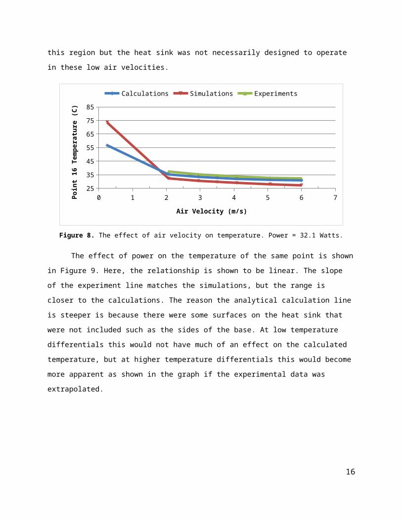
Figure 10. Drawings for manufacturing the heat sink.

19

Figure 11. Location of holes drilled for mounting thermocouples.

20

The point # in the following tables corresponds to the thermocouple number used in the experiments. Not all the thermocouples were used so some numbers are skipped.

Table 3. Analytical calculation results for each state compared.

Analytical Calculations T (C) Additional Calculations T (C)Point # 1 2 3 4 5 6 7 8 9 10 11 12

5 35.78 32.99 30.35 30.93 31.77 32.41 33.19 35.06 56.30 45.27 83.19 50.356 31.84 29.93 28.13 28.67 29.46 30.07 30.81 32.62 53.62 38.33 75.16 48.139 35.93 33.11 30.44 31.03 31.88 32.53 33.32 35.21 56.54 45.53 83.82 50.44

10 31.84 29.93 28.13 28.67 29.46 30.07 30.81 32.62 53.62 38.33 75.16 48.1314 33.96 31.58 29.33 29.90 30.73 31.37 32.14 34.00 55.22 42.07 79.86 49.3316 36.38 33.45 30.69 31.27 32.11 32.75 33.53 35.41 56.66 46.32 84.31 50.69

heater 102.33 84.66 67.96 68.55 69.39 70.04 70.82 72.69 94.0 162.4 200.5 88.0q (W) 56.8 44.1 32.1 32.1 32.1 32.1 32.1 32.1 32.1 100 100 32.1u (m/s) 6.00 6.00 6.00 5.07 4.08 3.50 2.95 2.06 0.25 6.00 0.75 6.00T∞ (C) 23.3 23.3 23.3 23.3 23.3 23.3 23.3 23.3 23.3 23.3 23.3 43.3

Table 4. Computational simulation results for each state compared.

ANSYS Icepak Simulation T (C) Additional Simulations T (C)Point # 1 2 3 4 5 6 7 8 9 10 11 12

1 30.85 29.55 28.33 28.96 29.70 30.27 31.02 32.75 73.55 35.25 79.88 47.252 32.73 31.01 29.39 30.06 30.84 31.46 32.27 34.11 75.38 38.56 85.17 47.574 28.21 27.11 26.08 26.68 27.41 27.95 28.57 29.97 69.77 31.93 73.49 45.00

5 30.04 28.53 27.12 27.79 28.58 29.21 30.02 31.81 72.65 35.14 80.85 45.816 27.37 26.46 25.60 25.99 26.31 26.77 27.46 28.89 67.12 30.45 67.39 44.827 32.73 30.63 28.64 29.40 30.26 30.89 31.69 33.39 74.23 39.89 85.91 47.019 29.21 27.89 26.65 27.29 28.06 28.61 29.31 31.10 72.79 33.70 79.64 45.22

10 29.60 28.20 26.87 27.48 28.20 28.81 29.59 31.28 70.09 34.38 76.49 45.7113 29.81 28.36 26.99 27.66 28.47 29.12 29.93 31.82 73.19 34.75 81.80 45.6914 28.62 27.43 26.31 26.93 27.64 28.20 28.89 30.24 72.04 32.65 76.68 45.2415 29.78 28.33 26.97 27.63 28.37 29.00 29.80 31.74 73.27 34.69 82.54 45.0816 30.45 28.86 27.35 28.06 28.92 29.61 30.47 32.42 73.64 35.88 83.74 45.97

q (W) 56.8 44.1 32.1 32.1 32.1 32.1 32.1 32.1 32.1 100 100 32.1u (m/s) 6.00 6.00 6.00 5.07 4.08 3.50 2.95 2.06 0.25 6.00 0.75 6.00T∞ (C) 23.3 23.3 23.3 23.3 23.3 23.3 23.3 23.3 23.3 23.3 23.3 43.3

21

Table 5. Experimentally measured temperatures for each trial.

Experimentally Measured T (C)Point # 1 2 3 4 5 6 7 8

1 32.89 31.38 29.53 30.06 31.01 31.66 32.48 34.452 33.26 31.70 29.79 30.35 31.32 31.94 32.75 34.783 29.59 28.69 27.53 28.15 29.27 29.89 30.59 32.534 29.73 28.84 27.64 28.04 28.75 29.20 29.80 31.325 35.44 33.86 31.92 32.50 33.49 34.16 35.00 37.066 29.35 28.54 27.44 27.89 28.71 29.24 29.93 31.697 36.17 34.19 31.77 32.31 33.25 33.90 34.74 36.658 26.93 26.56 25.84 25.87 26.82 26.86 27.46 29.349 32.51 31.08 29.31 29.80 30.68 31.26 32.01 33.84

10 32.43 31.01 29.27 29.81 30.74 31.39 32.24 34.2911 23.94 24.10 24.06 24.04 24.13 24.06 24.06 24.0812 24.26 24.42 24.38 24.37 24.47 24.42 24.41 24.4713 33.69 32.06 30.07 30.56 31.47 32.06 32.87 34.9714 30.50 29.41 28.02 28.55 29.50 30.16 30.96 32.9115 32.80 31.32 29.50 30.04 30.96 31.51 32.25 34.3316 36.13 34.38 32.24 32.80 33.81 34.49 35.33 37.4217 24.03 24.22 24.20 24.21 24.28 24.22 24.21 24.2118 23.72 23.51 23.50 23.61 23.85 24.19 24.44 24.66

heater 95.30 84.80 71.00 70.70 70.00 69.70 70.00 71.50q (W) 56.8 44.1 32.1 32.1 32.1 32.1 32.1 32.1f (Hz) 42.5 42.5 42.5 37.0 30.0 26.0 22.0 15.0u (m/s) 6.00 6.00 6.00 5.07 4.08 3.50 2.95 2.06T∞ (C) 23.3 23.3 23.3 23.3 23.3 23.3 23.3 23.3

22

Appendix B

Hand Calculations

23