ABSTRACT This study treats the design of secondary structures for wheel-loaded decks. It concludes that significant savings in structural weight, overall cost and environmental impact can be obtained by an improved design. The rules of three classification societies are examined and their principle differences are discussed. Weight and cost optimal solutions of rule-based design are identified for a deck of a typical short-sea RoRo-vessel. The rule-optimal designs are assessed and further improved on the basis of FE-calculations and the economic and environmental benefits associated with the best solutions are approximated.

TABLE OF CONTENTS Acknowledgements ....................................................................................................................................................... 1 Introduction ................................................................................................................................................................... 2

Overview .................................................................................................................................................................... 2 The reference ship .................................................................................................................................................... 2

Rule-based design .......................................................................................................................................................... 3 Design loads .............................................................................................................................................................. 4 Scantling requirements ............................................................................................................................................. 6

Plating ..................................................................................................................................................................... 6 Stiffeners ................................................................................................................................................................ 8 Special considerations (DNV) ..........................................................................................................................10 Corrosion additions ...........................................................................................................................................13

Rule-optimal scantlings ..........................................................................................................................................13 Preconditions ......................................................................................................................................................13 Scantlings calculation .........................................................................................................................................13 Weight and cost calculation ..............................................................................................................................14 Solutions ..............................................................................................................................................................15

Direct calculation .........................................................................................................................................................16 Global stresses .........................................................................................................................................................17 Local models ............................................................................................................................................................18 Acceptance criteria..................................................................................................................................................20

Effects on operation ...................................................................................................................................................22 Stability .....................................................................................................................................................................23 Power requirement .................................................................................................................................................23 Economy ..................................................................................................................................................................26 Environment............................................................................................................................................................27

Generalisation ..............................................................................................................................................................28 Discussion and conclusions .......................................................................................................................................29 References.....................................................................................................................................................................31

ACKNOWLEDGEMENTS I would like to express my sincere gratitude to my supervisors, Niels Georg Larsen and Anders Rosén, for their much valued guidance, critique and support. I would also like to extend my thanks to Vincenzo Cipriani and to Fabio Emolumento for their enthusiastic contributions in many long discussions and laborious exercises in FE-analysis.

- 1 -

INTRODUCTION This report is the result of a thesis project in Naval Architecture at the Royal Institute of Technology. The project was conducted in collaboration with the Danish ship design company Knud E. Hansen A/S (KEH) and for the main part at the company’s head office in Elsinore.

OVERVIEW RoRo-decks are different from other stiffened panels in ship structure in that the loads imposed by wheels of vehicles cannot be idealised as being uniformly distributed. The decks must be able to sustain the loads of wheels at all positions where they are likely to occur, but the structures must also be light as they constitute a relatively large part of the ship’s structural weight. The classification societies have chosen different approaches for idealizing the problem in their formulae for scantling requirements, which leads to the acceptance of different designs and it is therefore of interest for the designer to examine the differences between the rule requirements. A similarity with the design of other stiffened panels is that the requirements are based on input of the structural layout and materials, which are chosen by the designer. However, it is not obvious to the designer beforehand which combination of materials and spacings between members will result in a particularly light or cheap structure. These two aspects, the differences between rule requirements and the identification of optimal scantlings, are treated in the first chapter of this report, called Rule-based design. One deck of a typical RoRo-vessel is used as an example for the analyses.

In the second chapter, Direct calculation, a selection of the identified optimal designs are evaluated by use of the finite element method and possibilities of further reducing the scantlings are investigated.

The third chapter treats the Effects on operation associated with the alteration of the design, such as reduced fuel consumption and the corresponding impact on the ships economic value as well as the environment, due to a lower weight. The accumulated effects of applying the same methods for the design of the remaining decks are estimated in the fourth chapter called Generalisation, which is followed by a discussion and the conclusions of the study.

THE REFERENCE SHIP In this study, a typical short-sea RoRo-vessel is used as a reference for calculating the potential gains of an improved deck structure. The midship section is shown in Figure 1. The main deck is chosen for the examination because it is expected to be subjected to small global loads and the scantlings therefore to be driven by the special rules for wheel-loaded decks.

- 2 -

Figure 1. Midship section of the reference vessel.

The main deck is a double deck structure with so called ‘buoyancy boxes’, which is typical for this type of vessel. RoRo-decks are by necessity unobstructed along the length of the ship in order to allow the rolling on/off of cargo, which means there is no transverse subdivision by bulkheads as found in other types of cargo ships. The buoyancy boxes in the deck are therefore required for the ship’s safety in damaged conditions. The lower layer of plating is designed for withstanding water pressure in case the compartment is flooded, but it does not contribute to the local structure supporting the wheel loads. These loads are supported by the top layer of stiffened panel, as highlighted by the dotted marking in Figure 1, and it is the design of this part of the structure that is the subject of this study.

In order to assess how the performance of the vessel might be affected by an alteration of the deck scantlings, one must also consider a ‘reference transport scenario’. The reference vessel has previously been trafficking the route Gothenburg – Kiel on a schedule of six crossings per week (three in each direction) [1], a distance of 213 NM [2], which can be considered as an ordinary scenario for the type of vessel and is used as a basis for fuel cost estimations in this study.

RULE-BASED DESIGN In this chapter, the rules of three different class societies are examined and their respective optimal designs are compared with respect to weight and cost. The chosen class societies are Det Norske Veritas (DNV), Bureau Veritas (BV) and Registro Italiano Navale (RINA). DNV and RINA were chosen due to their special relevance for KEH; DNV is one of the most commonly employed class societies for KEH’s designs and RINA has been used to an increasing extent in recent projects. BV was chosen on the grounds that it was the first class society to implement the principles of LRFD (load and resistance factored design), as recognised by the Ship Structure Committee in [3]. The rules of BV and RINA are very similar due to their collaboration. However, there are differences which lead to a significant divergence of the scantling requirements.

In DNV, the applicable rules for the design of wheel-loaded deck structures are mainly found in the Additional Class rules for Passenger and Dry Cargo Ships [4], which treat the classification of ‘permanent decks for wheel loads’ (PWDK). Some reference is also made to the Main Class rules for Hull Structural

- 3 -

Design [5]. In BV and in RINA, the rules for strength check of plating and stiffeners ‘subjected to wheeled loads’ are found in separate articles within the Rules for the Classification of Ships [6, 7].

DESIGN LOADS The vehicles that are to be carried on the deck, as specified in the midship section drawing of the reference ship, with axle loads, wheel configurations and footprint dimensions, are shown in Figure 2 below. This data is used as input for calculating the design loads.

Figure 2. Load areas and axle loads of vehicles that are to be carried on the deck.

The formulae for calculating the design load according to each of the considered societies are given in Table 1. The design load according to DNV, equation (1), is expressed as a pressure, whereas the so called ‘wheeled force’ according to BV and RINA, equations (2) and (3), is a force. As it seems, DNV considers the load to be evenly distributed over the rectangular area of the tyre print, while neither BV nor RINA take the load area into consideration at this point.

Table 1. Rule formulas for calculation of design loads.

Society Design load formula Variables

DNV 𝑝 = 𝑄𝑛𝑜𝑎𝑏

(9.81 + 0.5𝑎𝑣) [kN/m2] (1)

Q no a b av

= maximum axle load in t = number of loads areas on the axle = extent in m of the load area parallel to the stiffeners = extent in m of the load area perpendicular to the stiffeners = 6/�𝑄for moving cargo handling vehicles, harbour conditions. = vertical acceleration as defined in Pt.3 Ch.1 Sec.4 for stowed vehicles, sea going conditions

BV 𝑃0 = 𝛾𝑆2𝐹𝑆 + 𝛾𝑊2𝐹𝑊,𝑍 [kN] (2) 𝛾𝑆2 𝐹𝑆

𝛾𝑊2 𝐹𝑊,𝑍

= partial safety factor - still water pressure = still water wheeled force = partial safety factor - wave pressure = inertial wheeled force

RINA 𝑃0 = 𝛾𝑆2𝐹𝑆 + 0.4𝛾𝑊2𝐹𝑊,𝑍 [kN] (3) 𝛾𝑆2 𝐹𝑆

𝛾𝑊2 𝐹𝑊,𝑍

= partial safety factor - still water pressure = still water wheeled force = partial safety factor - wave pressure = inertial wheeled force

- 4 -

The basic principle which is common to all of the design load formulae in Table 1 is Newton’s second law of motion, F = m∙a. The force that one wheel imposes on the structure is calculated by multiplying the mass supported on the wheel by an acceleration corresponding to the ship’s motions in the examined condition. The acceleration approximation for seagoing condition according to DNV is an extreme value, with a probability of exceedance of 10-8 during an operating life of 20 years in the North Atlantic [5]. BV and RINA do not explicitly state the probability of exceedance related to their acceleration approximations, but that accelerations that can be reached with a probability level of 10-5 should be determined if they are to be derived from direct calculations. The calculated values of the acceleration additions, av for DNV (seagoing condition) and aZ1 for BV and RINA, amidships of the reference vessel are given in Table 2.

Table 2. Vertical acceleration additions for cargo in the midship region of the reference vessel.

Society Vertical acceleration addition

DNV 𝑎𝑣 = 4.9829 𝑚/𝑠2

BV & RINA 𝑎𝑍1 = 3.6949 𝑚/𝑠2

While DNV’s av for seagoing condition is based on what appears to be an empirically derived relationship between the highest probable vertical acceleration and the length and speed of the vessel, the reasoning behind the expression for av in harbour condition is not as clear. Here the acceleration is inversely proportional to the square root of the axle load, i.e. a heavier axle is considered to be subjected to less acceleration. The underlying theory is not obvious, but a consequence is that the design load approximation of DNV differs more or less from those of BV and RINA depending on the magnitude of the axle load.

The ‘still water wheeled force’ FS is the same according to BV and RINA and is expressed

𝐹𝑆 = 𝑀 ∙ 𝑔 (4) where M is the mass supported by one wheel and g is the gravitational constant. The ‘inertial wheeled force’ FW,Z, however, is calculated differently by the two societies and the expressions for seagoing and harbour condition are given in Table 3.

Table 3. Formulae for "inertial wheeled force" according to BV and RINA.

Society Upright (seagoing) condition Harbour condition

BV 𝐹𝑊,𝑍 = 0.5𝑀𝑎𝑍1 𝐹𝑊,𝑍 = 0.1𝑀𝑔

RINA 𝐹𝑊,𝑍 = 𝑀𝑎𝑍1 𝐹𝑊,𝑍 = 0.5𝑀𝑎𝑍1

If the design pressure of DNV is converted into a point load, by omitting the tyre print area in equation (1), this load could also be expressed on the form ‘still water force + inertial force’ as

𝑃0 = 𝑀 ∙ 𝑔 + 0.5𝑀 ∙ 𝑎𝑣 (5) which is the same as BV’s equation (2) for seagoing condition, but without the safety factors. RINA’s inertial force in seagoing condition is 20 % lower than BV’s (the safety factors are the same), using a factor of 0.4 instead of 0.5 as both BV and DNV. In harbour condition, BV’s inertial force is expressed as 10 % of the gravitational force and RINA’s as 50 % of the seagoing inertial force.

Considering the specifications of vehicles in Figure 2, a representative axle for comparing the design loads could be taken as one which has two wheels and an axle load of 20 t. The calculated values for such an axle are given in Table 4.

- 5 -

Table 4. The design load of one wheel of a two-wheeled axle carrying 20 t.

Society Upright (seagoing) condition Harbour condition

DNV 123.0 kN 104.8 kN BV 120.3 kN 109.9 kN RINA 115.8 kN 107.0 kN

The design load approximation of DNV is 6 % higher than that of RINA in seagoing condition, while BV’s value is 5 % higher than DNV’s in harbour condition. All of the loads except DNV’s for harbour condition are proportional to the axle load and their relative differences will be the same for different axles, while DNV’s load for harbour condition increases (in relation to the others) with decreasing axle load. For an axle load of 2 t on two wheels, DNV’s value is 10 % higher than that of RINA.

SCANTLING REQUIREMENTS

Plating The formulae for plate thickness requirements according to each of the class societies are given in Table 5. DNV’s requirement is for the gross thickness, including the corrosion addition tk, while BV’s and RINA’s requirements are for the net thickness.

Table 5. Requirement formulae for plating.

Society Requirement on plating

DNV 𝑡 =

77.4𝑘𝑎�𝑘𝑤𝑐𝑠𝑝√𝑚𝜎

+ 𝑡𝑘 (6)

BV 𝑡 = 0.9𝐶𝑊𝐿�

𝑛𝑃0𝑘𝜆 (7)

RINA 𝑡 = 𝐶𝑊𝐿�𝑛𝑃0𝑘 − 𝑡𝑐 (8)

The thickness requirements of BV and RINA, equations (7) and (8), are not identical but they both contain a common basic expression that looks like

𝑡 = 𝐶𝑊𝐿�𝑛𝑃0𝑘 (9) The relationship between the material factor k and the yield stress of the material is defined by both societies as

𝜎𝑦 = 235𝑘

(10) Considering the case when the plate is subjected one point load, which gives n = 1 and CWL = 2, equation (9) can be reformulated as

𝑡 = �4∙235𝑃0𝜎𝑦

(11)

The relationship between thickness and stress described in equation (11) can be compared to the formula for the bending stress at the centre of the long edge of a rectangular plate, subjected to a uniform load over a small circular area at its centre, given in [8] as

𝜎𝑏 = 𝛽2𝑊𝑡2

(12)

- 6 -

Where β2 =1.008 for a plate with an aspect ratio greater than 2.0. P0 in equation (11) is expressed in kN, while t and σy are in mm and N/mm2 respectively. Converting into consistent units, the relationship between σb and σy can be expressed as

𝜎𝑏 = 1.072𝜎𝑦 (13) If the edges of the plate are fixed and the load P0 is a point load at the centre, a plate with thickness according to equation (11) will yield at the centres of its long edges. The bending stress calculated according to equation (12) is 7.2 % higher than the yield stress of the material. If the thickness is further

reduced by the factor 0.9�1𝜆 as in BV’s equation (7) the corresponding differences between yield stress

and bending stress at edges is 13.0 %.

RINA’s somewhat curious subtraction of tc in equation (8) entails that corresponding difference between yield stress and calculated stress is dependent on the relationship between the yield stress and the applied load. Taking W = 115800 N as the design load corresponding to 10 t in seagoing condition in Table 4, σy = 326.4 N/mm2 corresponding to the k-factor of A36-steel and tc = 0.5 mm, the difference between σy and σb is 13.4 %.

DNV’s formula for plate thickness, equation (6), includes a variable called ’allowable bending stress’, denoted σ. It is not explained in [4] why a bending stress of σ is allowable, but for fair evaluation σ is here expressed in terms of yield stress. σ is given as 320∙f1 for seagoing condition, while σy is expressed as 235∙f1, which gives σ = 1.36∙ σy. Disregarding the corrosion addition equation (6) can be expressed as

𝑡 = 77.4𝑘𝑎�𝑘𝑤𝑐𝑠𝑝1.36𝑚𝜎𝑦

(14)

where

𝑘𝑤 = 1.3 − 4.2

�𝑎𝑠+1.8�2 maximum 1.0 for a ≥ 1.94 s (15)

and

𝑚 = 38

�𝑏𝑠�2−4.7𝑏𝑠+6.5

for 𝑏𝑠 ≤ 1.0 (16)

Recognizing that c = b when b < s and that W in equation (12) corresponds to p∙a∙b∙10-3, equation (14) can be expressed on the form of equation (12) as

𝑡 = �(77.4𝑘𝑎)2𝑘𝑤∙10−3

1.36𝑚∙ 𝑠𝑎∙ 𝑊𝜎𝑦

(17)

Unlike the requirements of BV and RINA, equation (17) cannot be evaluated for a point load, since this entails division by zero. However, assuming that the load area is square, the smallest dimensions of the load area for which a plate designed according to equation (14) exhibits yielding at its edges according to equation (12), are found by solving 𝑎

𝑠 out of

(77.4𝑘𝑎)2𝑘𝑤∙10−3

1.36𝑚∙ 𝑠𝑎

= 𝛽2 (18)

where 𝑏

𝑠= 𝑎

𝑠 in m. This gives 𝑎

𝑠 = 0.042, which for the reference structure corresponds to 26 mm. For all

tyre prints that are larger than 26x26 mm, a plate with thickness according to equation (14) will exhibit yielding at its long edges if all edges are fixed.

- 7 -

It can be concluded from the above analysis that all of the examined thickness requirements either allow yielding or consider the boundaries of the plate to be less than fixed or both. It is not explained in the rules what theories the requirements are based on, nor is it obvious to the designer by comparing with formulae found in a common handbook.

Stiffeners The formulae for the requirements on stiffeners are given in Table 6. Also here, the requirement of DNV is for gross scantlings, including the corrosion addition wk, while the requirements of BV and RINA are for net scantlings.

Table 6. Requirement formulae for stiffeners.

Society Requirement on stiffeners

DNV 𝑍 =

1000𝑘𝑧𝑙𝑐𝑑𝑝𝑤𝑘𝑚𝜎 (19)

BV 𝑤 = 𝛾𝑅𝛾𝑚

𝛼𝑤𝑘𝑠𝑃0𝑙6�𝑅𝑦 − 𝛾𝑅𝛾𝑚𝜎𝑥1𝑊𝐻�

103 (20)

𝐴𝑆ℎ = 20𝛾𝑅𝛾𝑚𝛼𝑤𝑘𝑇𝑃0𝑅𝑦

(21)

RINA 𝑤 = 𝛾𝑅𝛾𝑚

𝛼𝑆𝑃0𝑙6�𝑅𝑦 − 𝛾𝑅𝛾𝑚𝜎𝑁�

103 (22)

𝐴𝑆ℎ = 20𝛾𝑅𝛾𝑚𝛼𝑤𝑘𝑇𝑃0𝑅𝑦

(23)

The requirements on section modulus, denoted Z by DNV and w by BV and RINA, all appear to be related to formulae for elastic bending of straight beams. Recognising that the relationship between section modulus, bending moment and bending stress is defined

𝑍 = 𝑀𝜎

(24) the terms that constitute the bending moment M can be extracted from each of the formulae. Omitting the corrosion addition in equation (19) and the safety factors and terms including global stresses in in equations (20) and (22), the approximation of the bending moment according to each society can be expressed as in Table 7.

Table 7. Bending moments corresponding to the requirement formulae.

Society Bending moment

DNV 𝑀 =

1000𝑘𝑧𝑙𝑐𝑑𝑝𝑚 (25)

BV 𝑀 =

𝛼𝑤𝑘𝑠𝑃0𝑙6 103 (26)

RINA 𝑀 =

𝛼𝑆𝑃0𝑙6 103 (27)

The formulae for calculating the maximum bending moment of a beam subjected to a central point load are given in [9] as

- 8 -

𝑀 = 𝐹𝑙4

(28) for simply supported ends and

𝑀 = 𝐹𝑙8

(29) for fixed ends. The point force F is represented by cdp in equation (25) and by P0 in equations (26) and (27), and the factor 103 in all three equations is just a conversion of units. Assuming that the load is one point load, i.e. that the dimensions of the load area are zero, the coefficients kz, m, αw, ks and αs can be defined and equations (25) to (27) can be expressed as in Table 8.

Table 8. Bending moments corresponding to the requirement formulae when considering a point load.

Society Bending moment

DNV 𝑀 =

𝐹𝑙4.46 (30)

BV 𝑀 =

𝐹𝑙6 (31)

RINA 𝑀 =

𝐹𝑙6 (32)

As it appears when comparing the equations in Table 8 with equations (28) and (29), the requirement of DNV seems to be based on end conditions that are quite close to simply supported, while BV’s and RINA’s seem to be based on end conditions that are half-way between simply supported and fixed. The approach of DNV is more conservative in this respect. The safety factors of BV and RINA are equal and their value is 1.04. The allowable stress in equation (19) is defined as 160∙f1 (seagoing), while the yield stress is 235∙f1, which means DNV’s safety factor against yielding can be considered to be 1.47 for comparison with BV and RINA.

The coefficient kz in equation (19) reduces the bending moment if the width of the tyre print exceeds 60 % of the stiffener spacing, so as to consider the loadbearing contribution of adjacent stiffeners, and c limits the width of the load area to a maximum of one stiffener spacing, implying that loadbearing width of the stiffener is equal to the stiffener spacing. In the axial direction, the factor m increases with the length of the tyre print up to a maximum of 12 when the length of the load area is greater than 3.5 stiffener spans, which gives the exact same expression as the formula for maximum bending moment in a beam fixed at both ends and subjected to a uniform load:

𝑀 = 𝑄𝐿12

(33) The requirements of BV and RINA do not consider this relationship between load area and bending moment. The load of one tyre is strictly considered as a point load, which is especially conservative for wide tyre prints, since it implies that one stiffener must support the entire load without any contribution from adjacent stiffeners.

The coefficient ks in equation (20) takes into account the increase of the bending moment, as a function of the distance between axles, when one stiffener supports two axles along its length. DNV’s equation (19) does not include such a coefficient, but DNV instead requires the designer to especially consider cases when a member is subjected to more than one load along its length. This calculation is treated in the next section. BV’s coefficient αw takes into account the distances between wheels in a wheel group so that the load imposed by each wheel is related to the wheel’s proximity to the examined stiffener, as described in

- 9 -

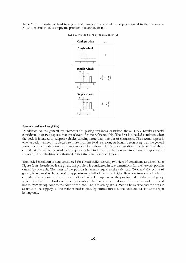
Table 9. The transfer of load to adjacent stiffeners is considered to be proportional to the distance y. RINA’s coefficient αs is simply the product of ks and αw of BV.

Table 9. The coefficient αW, as provided in [6].

Configuration αW

Single wheel

1

Double wheels

Triple wheels

Special considerations (DNV) In addition to the general requirements for plating thickness described above, DNV requires special consideration of two aspects that are relevant for the reference ship. The first is a heeled condition when the deck is intended to support vehicles carrying more than one tier of containers. The second aspect is when a deck member is subjected to more than one load area along its length (recognising that the general formula only considers one load area as described above). DNV does not dictate in detail how these considerations are to be made – it appears rather to be up to the designer to choose an appropriate approach. The calculations performed in this study are described below.

The heeled condition is here considered for a Mafi-trailer carrying two tiers of containers, as described in Figure 3. As the axle loads are given, the problem is considered in two dimensions for the heaviest portion carried by one axle. The mass of the portion is taken as equal to the axle load (30 t) and the centre of gravity is assumed to be located at approximately half of the total height. Reaction forces at wheels are considered as a point load at the centre of each wheel group, due to the pivoting axle of the wheel group which distributes the load evenly on both sides. The trailer is centred in a three metres wide lane and lashed from its top edge to the edge of the lane. The left lashing is assumed to be slacked and the deck is assumed to be slippery, so the trailer is held in place by normal forces at the deck and tension at the right lashing only.

- 10 -

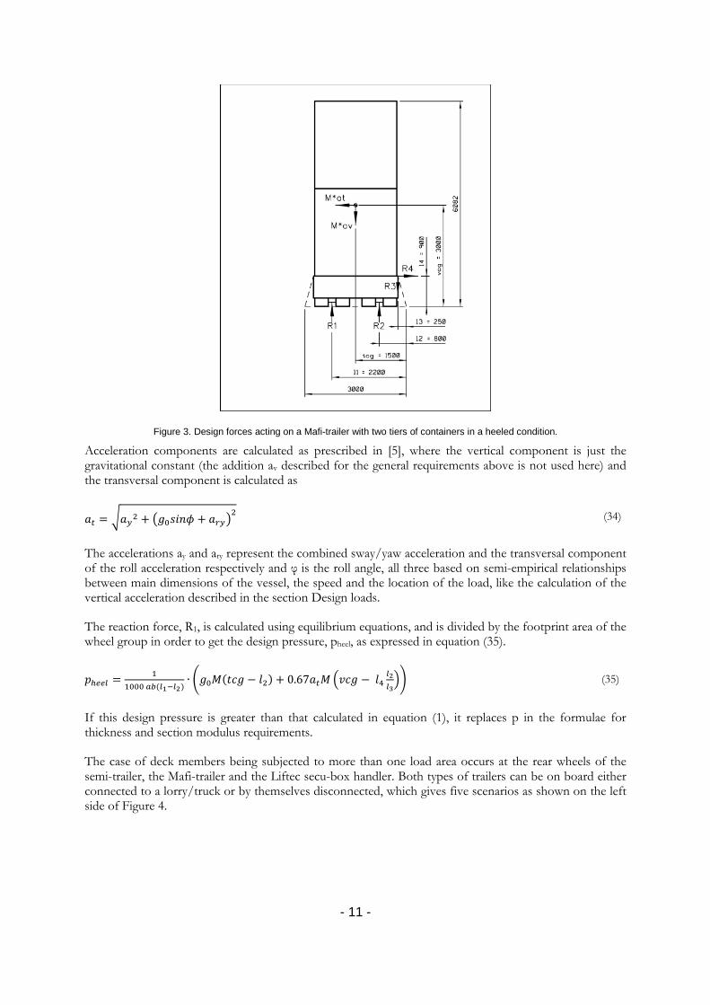
Figure 3. Design forces acting on a Mafi-trailer with two tiers of containers in a heeled condition.

Acceleration components are calculated as prescribed in [5], where the vertical component is just the gravitational constant (the addition av described for the general requirements above is not used here) and the transversal component is calculated as

𝑎𝑡 = �𝑎𝑦2 + �𝑔0𝑠𝑖𝑛𝜙 + 𝑎𝑟𝑦�2 (34)

The accelerations ay and ary represent the combined sway/yaw acceleration and the transversal component of the roll acceleration respectively and φ is the roll angle, all three based on semi-empirical relationships between main dimensions of the vessel, the speed and the location of the load, like the calculation of the vertical acceleration described in the section Design loads.

The reaction force, R1, is calculated using equilibrium equations, and is divided by the footprint area of the wheel group in order to get the design pressure, pheel, as expressed in equation (35).

𝑝ℎ𝑒𝑒𝑙 = 11000 𝑎𝑏(𝑙1−𝑙2)

∙ �𝑔0𝑀(𝑡𝑐𝑔 − 𝑙2) + 0.67𝑎𝑡𝑀 �𝑣𝑐𝑔 − 𝑙4𝑙2𝑙3�� (35)

If this design pressure is greater than that calculated in equation (1), it replaces p in the formulae for thickness and section modulus requirements.

The case of deck members being subjected to more than one load area occurs at the rear wheels of the semi-trailer, the Mafi-trailer and the Liftec secu-box handler. Both types of trailers can be on board either connected to a lorry/truck or by themselves disconnected, which gives five scenarios as shown on the left side of Figure 4.

- 11 -

Figure 4. Load cases when a stiffener is subjected to more than one load area along its length.

Each scenario is idealised as a two-dimensional beam subjected to point loads and boundary conditions, as shown on the right side of Figure 4. The boundary conditions are idealised as either fixed or simply supported depending on loads on adjacent spans.

The point loads are calculated by multiplying the design pressure by the footprint area. However, if the width of the footprint is greater than the stiffener spacing, the load area is reduced to the width of the stiffener spacing in order to only consider the loads supported by one stiffener. Membrane forces in the plating are neglected.

The idealised beam systems are statically indeterminate. These are solved for the maximum bending moment by use of a simple beam analysis software [10] based on the direct stiffness method. In order to determine the worst possible placement of the loads, the calculation is iterated through the full range of when one span is subjected to two loads, as illustrated in Figure 5, and the placement corresponding to the highest maximum bending moment is determined.

Figure 5. The bending moment diagram of the first model in Figure 4, for all positions when the middle span is subjected to the two rearmost axles.

Knowing the maximum bending moment, the section modulus requirement is formulated as

𝑍 = 1000 𝑀𝜎

(36)

- 12 -

where M is the maximum bending moment, σ is the same allowable stress as used in equation (19) and the factor 1000 is for conversion into cm3 as used by DNV. If the value obtained from equation (36) is greater than that from (19), it is taken as the requirement for the stiffener section modulus.

Corrosion additions As mentioned earlier in this chapter, the societies have different approaches for considering corrosion additions and DNV’s scantling requirements are for gross scantlings while BV’s and RINA’s are for net scantlings. There is also a difference in the way that the class societies prescribe corrosion additions. The examined structure does not fit into any of the categories for which the societies prescribe specific corrosion additions. In such cases BV and RINA require a general corrosion addition of tc = 0.5 mm, while DNV prescribe that tk = 0.

RULE-OPTIMAL SCANTLINGS The scantling requirements on plating and stiffeners, given in Table 5 and Table 6, are dependent of general data of the ship, the loads, the structural arrangement and the materials used in the deck as input. Any deck design that is to be accepted by one of the societies based on rule-calculations must fulfil the scantling requirements set by every relevant design load in Figure 2. This part of the study is aimed at identifying the best deck designs that fulfil the requirements, with respect to weight and cost. The approach is based on iterating the requirement calculations for all materials and stiffener spacings to be considered, evaluating the weight and cost of each solution and thereafter selecting the best solutions.

Preconditions All input that is required for the rule calculations and is not directly related to the secondary structure of the examined deck, is based on values of the reference ship. Stiffener spacings are tested from 300 mm to 800 mm in steps of 10 mm. All five steel classes recognised by DNV are considered to be available and for designs based on DNV, plating and stiffeners of different steel classes are allowed to be combined freely. For designs based on BV and RINA, plating and stiffeners are required to be of the same material since this is specifically dictated by the rules. Stiffener profiles are selected from a limited list of HP-bulbs, given in Table 10, which may be considered to be normally available at European shipyards. The requirements obtained from the calculations are directly converted into the closest scantlings that fulfil them, by rounding the thickness requirement up to the closest 0.5 mm and selecting the smallest stiffener profile to fulfil the section modulus requirement.

Table 10.Section properties of normally available HP-profiles, acquired from [11].

Dimensions [mm]

Cross-section area [cm2]

Second moment of area [cm4]

Section modulus [cm3]

120 6 9.31 133 18.4 140 6.5 11.7 228 27.3 160 7 14.6 373 38.6 180 8 18.9 609 55.9 200 8.5 22.6 902 74.0 220 9 26.8 1296 95.3 240 9.5 31.2 1800 123 260 10 36.1 2477 153 280 10.5 41.2 3223 184 300 11 46.7 4190 222 320 11.5 52.6 5370 266 340 12 58.8 6760 313 370 12.5 67.8 9213 390 400 13 77.4 12280 476 430 14 89.7 16460 594

Scantlings calculation All of the rules that are required for the determination of plate and stiffener scantlings of the examined deck are programmed into a routine, which calculates the requirements for all defined load cases and a series of different stiffener spacings and materials as described above. In the case of DNV, results from an

- 13 -

old calculation spread sheet from DNV (Nauticus Hull – Wheel Loads v.9.00.2) were used for verification. The input in the spread sheet consisted of Lpp, L, D, Cb, V, Zn, f2b, f2d and axle loads and load area dimensions for seven different vehicles and the calculations had been performed for seven different stiffener spacings and one material factor. The results were presented as design pressure, allowable stress for plating, thickness requirement, allowable stress for stiffeners and section modulus requirement, for all seven vehicles for each stiffener spacing (i.e. 42 rows of results). Using the same input in the programmed routine returned the same results as given by the spread sheet. Unfortunately, no such spread sheet was available for verification of the codes for BV and RINA.

The section modulus requirement of DNV includes the effective flange contributed by the plating. Appendix B of [12] provides a table of calculated section moduli for HP-profiles including 600 mm wide plates. Matching results were obtained by using the parallel axis theorem for combining the section modulus provided in the profile table with a thin plate. In further calculations the effective flange is assumed to be equal to the stiffener spacing.

Weight and cost calculation The weight and cost of each deck design is at this stage evaluated ‘per metre at midship’. The metre-weight is obtained by multiplying the combined cross section area of plating and stiffeners by the density of steel.

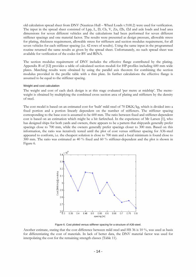
The cost model is based on an estimated cost for ‘built’ mild steel of 70 DKK/kg, which is divided into a fixed portion and a portion linearly dependent on the number of stiffeners. The stiffener spacing corresponding to the base cost is assumed to be 600 mm. The ratio between fixed and stiffener-dependent cost is based on an estimation which might be a bit farfetched. In the experience of Mr Larsen [1], who has designed ships for both yards and owners, there appears to be a pattern that shipyards generally prefer spacings close to 700 mm, while the owners generally prefer spacings closer to 300 mm. Based on this information, the ratio was iteratively tested until the plot of cost versus stiffener spacing for A36-steel appeared to conform, i.e. the cheapest solution is close to 700 mm and a local minimum is found close to 300 mm. The ratio was estimated as 40 % fixed and 60 % stiffener-dependent and the plot is shown in Figure 6.

Figure 6. Cost plotted versus stiffener spacing for a structure of A36-steel.

Another estimate, stating that the cost difference between mild steel and HS 36 is 10 %, was used as basis for differentiating the cost of materials. In lack of better data, the DNV material factor was used for interpolating the cost for the remaining strength classes (Table 11).

- 14 -

Table 11.Estimated costs of steel at 600 mm stiffener spacing.

Material Material factor

Cost [DKK/kg]

A 1.00 70.00 A 27 1.08 71.44 A 32 1.28 75.03 A 36 1.39 77.00 A 40 1.47 78.44

The described cost model is very simple and likely quite inaccurate, mainly due to the general lack of cost data and the unreliability of the estimates. As stated in [13], this type of data is protected by the shipyards for commercial reasons and it is also of such a nature that it gets outdated quickly, which makes it difficult for any design company to keep track. However, it should be noted that the purpose of this cost model is not to make very accurate cost estimates for building a deck. The cost evaluation is used for ranking different designs against one another and for estimating the differences between the costs of the examined designs and the reference ship, not for estimating the total cost of any specific design.

Solutions The routine described above returns one solution for each combination of stiffener spacing, plating material and stiffener material that is used as input. The solutions are evaluated in terms of weight and cost as described in the previous section, which makes it possible to plot them according to weight and cost as shown in Figure 7.

Figure 7.Weights and costs of DNV-based solutions for spacings 300 to 800 mm (steps of 10 mm) and all steel classes. The red point represents the reference deck.

It is intuitive that the solutions of interest are those close to the bottom (cheap) and the left edge (light). More specifically, any solution for which there is no other solution that is both cheaper and lighter, is a “good” solution. These solutions are the so called Pareto-optimal solutions, and are marked in Figure 7 by an interconnecting line forming the ‘Pareto-frontier’. The Pareto-optimal solutions are found by using a “direct search approach”[14], in which each solution is compared to all other solutions and disregarded if any other solution turns out to be better in both respects (weight and cost). The Pareto-frontiers of all three societies are plotted together in Figure 8, where also the reference deck is included for comparison.

- 15 -

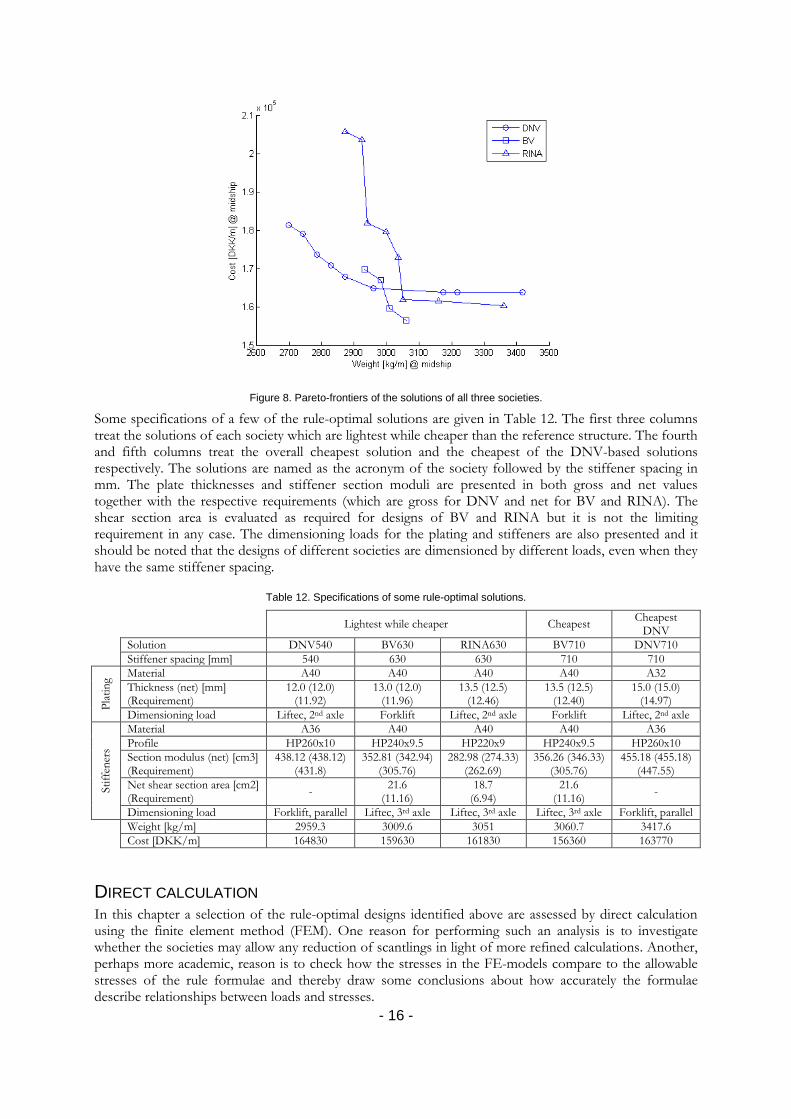
Figure 8. Pareto-frontiers of the solutions of all three societies.

Some specifications of a few of the rule-optimal solutions are given in Table 12. The first three columns treat the solutions of each society which are lightest while cheaper than the reference structure. The fourth and fifth columns treat the overall cheapest solution and the cheapest of the DNV-based solutions respectively. The solutions are named as the acronym of the society followed by the stiffener spacing in mm. The plate thicknesses and stiffener section moduli are presented in both gross and net values together with the respective requirements (which are gross for DNV and net for BV and RINA). The shear section area is evaluated as required for designs of BV and RINA but it is not the limiting requirement in any case. The dimensioning loads for the plating and stiffeners are also presented and it should be noted that the designs of different societies are dimensioned by different loads, even when they have the same stiffener spacing.

Table 12. Specifications of some rule-optimal solutions.

Lightest while cheaper Cheapest Cheapest DNV

Solution DNV540 BV630 RINA630 BV710 DNV710 Stiffener spacing [mm] 540 630 630 710 710

Plat

ing Material A40 A40 A40 A40 A32

Thickness (net) [mm] (Requirement)

12.0 (12.0) (11.92)

13.0 (12.0) (11.96)

13.5 (12.5) (12.46)

13.5 (12.5) (12.40)

15.0 (15.0) (14.97)

Dimensioning load Liftec, 2nd axle Forklift Liftec, 2nd axle Forklift Liftec, 2nd axle

Stiff

ener

s

Material A36 A40 A40 A40 A36 Profile HP260x10 HP240x9.5 HP220x9 HP240x9.5 HP260x10 Section modulus (net) [cm3] (Requirement)

438.12 (438.12) (431.8)

352.81 (342.94) (305.76)

282.98 (274.33) (262.69)

356.26 (346.33) (305.76)

455.18 (455.18) (447.55)

Net shear section area [cm2] (Requirement) - 21.6

(11.16) 18.7

(6.94) 21.6

(11.16) -

Dimensioning load Forklift, parallel Liftec, 3rd axle Liftec, 3rd axle Liftec, 3rd axle Forklift, parallel Weight [kg/m] 2959.3 3009.6 3051 3060.7 3417.6 Cost [DKK/m] 164830 159630 161830 156360 163770

DIRECT CALCULATION In this chapter a selection of the rule-optimal designs identified above are assessed by direct calculation using the finite element method (FEM). One reason for performing such an analysis is to investigate whether the societies may allow any reduction of scantlings in light of more refined calculations. Another, perhaps more academic, reason is to check how the stresses in the FE-models compare to the allowable stresses of the rule formulae and thereby draw some conclusions about how accurately the formulae describe relationships between loads and stresses.

- 16 -

GLOBAL STRESSES The stresses due to bending of the longitudinal hull girder are expected to be low, considering the proximity of the examined deck to the neutral axis of the hull girder. The normal stress induced by vertical bending at the height of the examined deck may be approximated according to BV as

𝜎1 = 𝑀𝑆𝑊+𝑀𝑊𝑉𝑍𝐴

10−3 (37)

where MSW and MWV are the still water and wave bending moments respectively and Za is the section modulus of the hull girder at the height of the deck. Evaluating equation (37) with values of the reference ship gives a normal stress of 26.7 N/mm2. This is here considered to be a low stress and for modelling simplicity this stress is neglected in the FE-analysis.

Observing the wide span of the deck, unsupported by bulkheads or pillars in the midship region as shown in Figure 1, it might be of interest to examine stresses induced by global deflection of the deck in the transverse plane when heavily loaded. These stresses are here approximated by applying a severe load on the global structure, which may be present simultaneously as the local structure is subjected to its most severe local load. The severe case is based on the scenario when Mafi-trailers with maximum load are parked on all four lanes of one side of the deck.

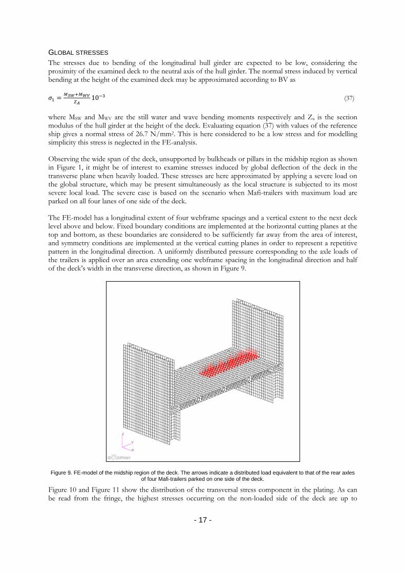
The FE-model has a longitudinal extent of four webframe spacings and a vertical extent to the next deck level above and below. Fixed boundary conditions are implemented at the horizontal cutting planes at the top and bottom, as these boundaries are considered to be sufficiently far away from the area of interest, and symmetry conditions are implemented at the vertical cutting planes in order to represent a repetitive pattern in the longitudinal direction. A uniformly distributed pressure corresponding to the axle loads of the trailers is applied over an area extending one webframe spacing in the longitudinal direction and half of the deck’s width in the transverse direction, as shown in Figure 9.

Figure 9. FE-model of the midship region of the deck. The arrows indicate a distributed load equivalent to that of the rear axles of four Mafi-trailers parked on one side of the deck.

Figure 10 and Figure 11 show the distribution of the transversal stress component in the plating. As can be read from the fringe, the highest stresses occurring on the non-loaded side of the deck are up to

- 17 -

approximately 15 MPa close to webframes and up to 7.5 MPa at midway between webframes. Also these stresses are here regarded as low and are therefore neglected in the analysis of the secondary structure.

Figure 10. Transversal stress due to the deflection caused by vehicles on deck. Values are in N/mm2.

Figure 11. A closer look at transversal stress in the plating. Values are in N/mm2.

LOCAL MODELS The analysis of stresses occurring in the plating is based on small models, extending three stiffener spacings in the transverse direction and one webframe spacing in the longitudinal direction as illustrated by the ‘small model’ in Figure 12. Shell elements are used to represent the plating, the two stiffeners are represented by bar elements with offset and fixed boundary conditions are imposed on all four edges.

Figure 12. Geometrical extents of FE-models considered for the analysis of plating.

- 18 -

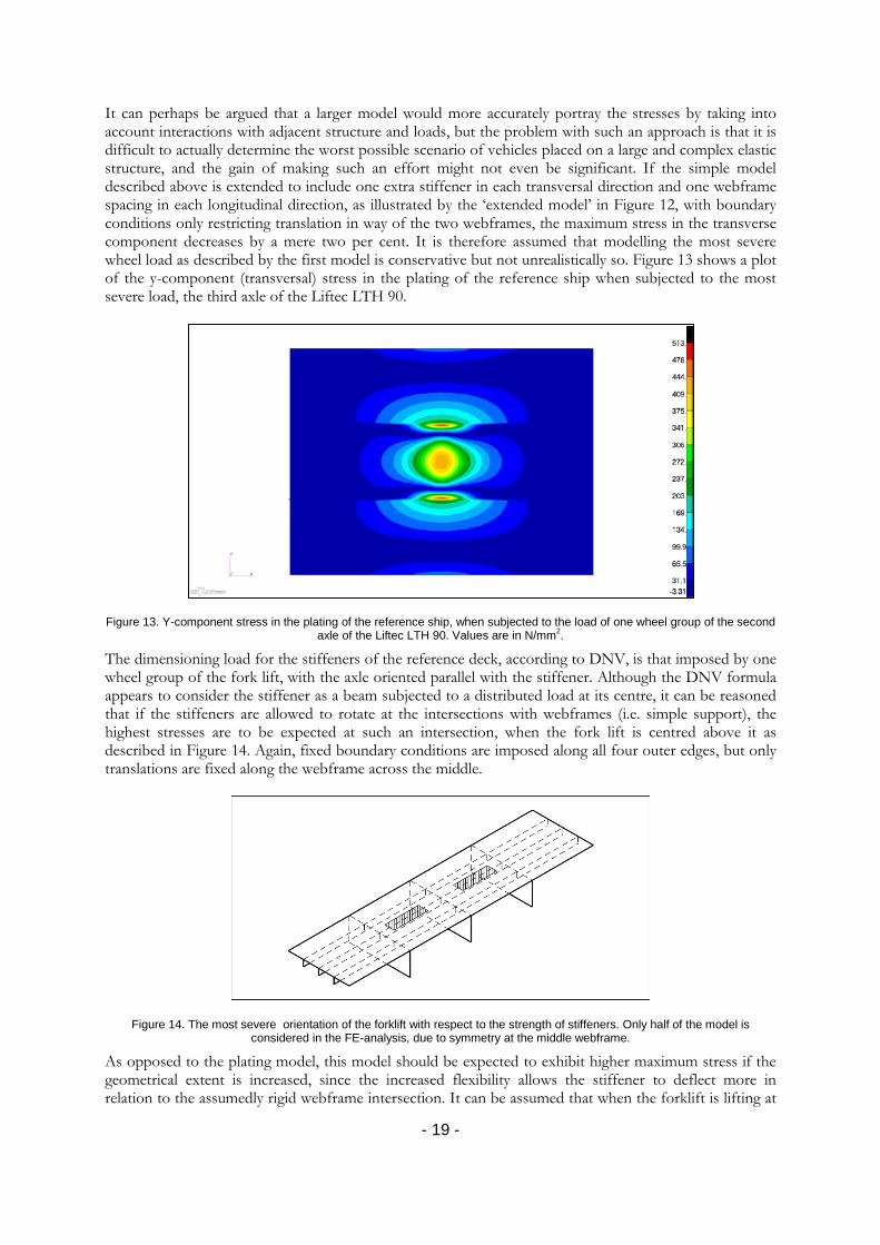
It can perhaps be argued that a larger model would more accurately portray the stresses by taking into account interactions with adjacent structure and loads, but the problem with such an approach is that it is difficult to actually determine the worst possible scenario of vehicles placed on a large and complex elastic structure, and the gain of making such an effort might not even be significant. If the simple model described above is extended to include one extra stiffener in each transversal direction and one webframe spacing in each longitudinal direction, as illustrated by the ‘extended model’ in Figure 12, with boundary conditions only restricting translation in way of the two webframes, the maximum stress in the transverse component decreases by a mere two per cent. It is therefore assumed that modelling the most severe wheel load as described by the first model is conservative but not unrealistically so. Figure 13 shows a plot of the y-component (transversal) stress in the plating of the reference ship when subjected to the most severe load, the third axle of the Liftec LTH 90.

Figure 13. Y-component stress in the plating of the reference ship, when subjected to the load of one wheel group of the second axle of the Liftec LTH 90. Values are in N/mm2.

The dimensioning load for the stiffeners of the reference deck, according to DNV, is that imposed by one wheel group of the fork lift, with the axle oriented parallel with the stiffener. Although the DNV formula appears to consider the stiffener as a beam subjected to a distributed load at its centre, it can be reasoned that if the stiffeners are allowed to rotate at the intersections with webframes (i.e. simple support), the highest stresses are to be expected at such an intersection, when the fork lift is centred above it as described in Figure 14. Again, fixed boundary conditions are imposed along all four outer edges, but only translations are fixed along the webframe across the middle.

Figure 14. The most severe orientation of the forklift with respect to the strength of stiffeners. Only half of the model is considered in the FE-analysis, due to symmetry at the middle webframe.

As opposed to the plating model, this model should be expected to exhibit higher maximum stress if the geometrical extent is increased, since the increased flexibility allows the stiffener to deflect more in relation to the assumedly rigid webframe intersection. It can be assumed that when the forklift is lifting at

- 19 -

its maximum capacity, there will not be another load significantly effecting adjacent structure, because this space would be occupied by the cargo on the forklift and the manoeuvring space required. For instance, the length of a 40’ container corresponds to about five webframe spacings. It can also be noted from Figure 15 that no significantly high stresses occur at the boundaries of the model (except at the symmetry cut), which suggests that the maximum stress is not likely to change if the extent is increased.

Figure 15. Von Mises stress in plating when subjected to a forklift wheel directly on top of a stiffener. Values are in N/mm2.

ACCEPTANCE CRITERIA The model in Figure 13 represents the structure of the reference ship subjected to the load of one wheel group of the second axle of the Liftec LTH 90 (counting from left to right in Figure 2), which was identified as the most severe load for plating with the given stiffener spacing. As can be read from the colour scale in Figure 13, the highest stress exceeds the yield stress of the material (355 MPa). For direct calculation of the plating, DNV allows a maximum bending stress of 320*f1 for seagoing conditions and 370*f1 for harbour conditions, the same allowable stresses as used in the general formula for plate thickness [15]. This gives a criterion of 514.3 MPa for the A36-steel of the reference structure, which is very close to the maximum y-component stress in the model. It can be verified that the y-component stress mainly consists of bending stress by finding that the stress on the opposite surface of the plate is very similar but with opposite sign, and the average of the two (the membrane stress) is less than 4.4 MPa.

The maximum bending stress in the plating, which is found close to the stiffeners, does not converge at moderate mesh densities due to the sharp connection between the shell and beam elements here. An element size of 10 mm is therefore chosen, since it is close to the thicknesses of both the plating and the stiffener web. A denser mesh would only return unrealistically high stresses because of the model simplicity. It should be noted that the maximum stress is already unrealistic, because it is beyond the yield limit of the material and therefore outside the scope of what can be accurately assessed with linear FEM – the obtained value can only be used for comparison with the criterion.

Also for the stiffeners, DNV permit the same allowable stress as used in the rule formula when performing direct calculations, i.e. 160*f1 for seagoing condition and 180*f1 for harbour condition. The criterion in this case is 250.2 MPa and the stress obtained from the model is 93.8 MPa.

Neither BV nor RINA have any acceptance criteria for FEM assessment of the secondary structure. However, there are ‘checking criteria’ for the bending and shear stress in stiffeners to be found in the same section as the requirement formulae, which are here used for comparison with stresses in the FE-models. The expressions are identical for both societies:

𝑅𝑦𝛾𝑅𝛾𝑚

≥ 𝜎 (38)

- 20 -

and

0.5 𝑅𝑦𝛾𝑅𝛾𝑚

≥ 𝜏 (39)

No comparable expression for the allowable stress in plating is found in the analysis in the aforementioned section, hence stresses in plating of BV and RINA based models are here compared to the allowable stress of DNV. Scantlings are not reduced on BV and RINA designs since it is simply not allowed.

EVALUATION AND IMPROVEMENT

The description of local models above refers to the dimensioning loads of the reference deck according to the rules of DNV. At another look at Table 12 it can be noted that the dimensioning loads of the designs are different. This could perhaps be expected, since the rules seem to be based on different idealisations of the structure. Recognising that the stiffener spacing of the BV solution is the same as that of the reference deck, but that the dimensioning load is different for both plating and stiffeners, the BV-based structure is tested for the dimensioning loads of both societies in order to determine which loads are more severe. In both cases, plating and stiffeners, it is found that the dimensioning load according to DNV is more severe.

In the case of stiffeners, a simple explanation can be found in that DNV requires some cargo handling vehicles to be additionally considered when oriented in the transverse direction of the ship (i.e. with axles oriented parallel to longitudinal stiffeners). Reasonable as this may seem, considering that a forklift might move around in all directions on a deck, this requirement was not found explicitly stated in the rules of BV. In order to implement this case, the designer must realise that αW, the “coefficient taking account of the number of wheels per axle considered as acting on the stiffener” [6], should be taken as one according to Table 9 when actually all three wheels of the group are centred over the stiffener, and that two wheels in a group should be considered as “double axles” [6] in the corresponding table for KS and KT. Even then, it is not obvious how a group of three wheels should be treated, since there are no formulae for KS and KT corresponding to triple axles. The said considerations have not been implemented in this study. No similarly simple explanation was found for the different dimensioning loads for plating.

In light of the above, the dimensioning load according to DNV is assumed to be the most severe load also for designs of BV and RINA. The results of some of the rule-optimal designs are summarised in Table 13.

Table 13. Evaluations of FE-models.

Rule-optimal designs Direct calc. designs

Ref ship DNV540 DNV710 BV630 BV710 RINA630 DNV540D DNV710D

Plat

ing

Max. bending [MPa] (Allowable DNV)

516 (514.3)

582 (543.9)

461 (473.6)

663 (543.9)

688 (543.9)

581 (543.9)

527 (543.9)

428 (473.6)

Bending @ centre [MPa] 444 450 408 560 581 526 473 428 Max. Von Mises [MPa] (Yield limit)

463 (355)

520 (390)

415 (315)

595 (390)

618 (390)

525 (390)

477 (390)

415 (315)

Deflection [mm] 8.45 6.75 9.03 12 15.2 11.3 7.8 10.2

Stiff

ener

s Max. bending [MPa] (Allowable)

93.8 (250.2)

96.6 (250.2)

104 (250.2)

139 (332.17)

143 (332.17)

181 (332.17)

211 (250.2)

225 (250.2)

Max. shear [MPa] (Allowable)

46.9 (-)

48.3 (-)

52 (-)

69.7 (166.08)

71.6 (166.08)

90.3 (166.08)

106 (-)

112 (-)

Deflection [mm] 1.38 1.43 1.41 2.13 2.15 2.84 3.53 3.52

The stresses in plating of the DNV-based designs are quite close to the allowable stresses, especially for the reference deck. The stresses in stiffeners on the other hand are much lower than their allowable values. A possible explanation might be found in DNV’s conservative boundary conditions, as described in the chapter Rule-based design. The boundary conditions of the DNV formula are close to simply supported at both ends and the load is centred, whereas in the FE-model one end of the stiffener is fixed and the load is off-centre. The plating of the RINA solution also exhibits bending stress close to the

- 21 -

allowable limit of DNV, even though it is tested at a higher load than it was dimensioned by. The platings of the BV solutions, on the other hand, exhibit much higher stresses. Also in the designs based on BV and RINA, the bending stresses in stiffeners are found to be low, although a bit higher than in the DNV-based designs. Here, part of the explanation is likely to be found in that the dimensioning load, the rearmost axles of the Liftec (see Table 12 and Figure 2), have wide tyre prints, but as suggested in the section Scantling requirements, the support from adjacent stiffeners is neglected by the rules.

Again, it should be noted that the solutions of BV and RINA are evaluated on basis of their net scantlings. A significant increase in strength should be expected due to the addition of a corrosion margin, as compared to the DNV solutions which do not require this addition.

For the rule-optimal solutions of DNV, the scantlings are here adjusted so that they exhibit stresses below the allowable limits by the smallest possible margins. In both cases the stress in the plating of the rule-based design exceeds the allowable stress and intuitively one might attempt to reduce the stress in the plating by increasing the plate thickness. However, another approach could be to reduce the stiffness of the stiffeners in order to even out the load distribution. The stiffener model of DNV540 allows reduction of the profile to HP200x8.5, which, implemented in the plating model, gives a maximum bending stress of 527 MPa in the plate. The modified solution is named DNV540D in Table 13. Likewise, DNV710D is obtained by reducing the stiffener profile of DNV710 to the same HP200x8.5. Plate thickness is not changed in either case. The impact on both weight and cost is quite high, which is illustrated in Figure 16 where the two solutions are plotted together with the rule-optimal solutions.

Figure 16. DC-improved solutions DNV540D and DNV710D plotted together with rule-optimal solutions.

It can also be noted that the distance from the rule-optimal solution is greater for DNV540D than for DNV710D, even though the stiffener profiles were reduced equally. This is simply because DNV540D has a greater number of stiffeners. The weight reduction in the case of DNV540D is 7 % and the cost reduction is also 7 %, compared to the rule-optimal design.

EFFECTS ON OPERATION The weight-difference (as compared to the reference deck) of each of the rule-optimal solutions and the two DC-improved solutions are given in Table 16. The greatest weight saving according to the table is about 80 t, which is close to the weight of one SECU-box, 95 t. However, considering the type of vessel that is examined and that it was designed to meet a certain cargo flow requirement, it is here assumed that a change in lightweight of this magnitude will not affect the payload. The vessel is what is referred to in [13] as an area based design, which means that its capacity is likely limited by the deck area rather than weight. Increasing the weight capacity would at best allow the replacement of a light vehicle by a heavier

- 22 -

one, but even that is unlikely in practice, since the vessel runs on a fixed schedule and must take whatever cargo mix there is.

STABILITY A change in the weight distribution of a ship structure affects the stability of the vessel and, in some loading conditions, the amount of ballast water that is needed in order to obtain sufficient stability. Examining a stability calculation for the reference vessel when fully loaded with SECU-boxes [16], it is found that the vertical location of the centre of gravity, KG, is at 11.318 m above the baseline, which is higher than the location of the examined deck (8.7 m). Therefore, a reduction of weight at the height of the deck will cause the centre of gravity to move upwards, which reduces the metacentric height, GM, in the expression

𝐺𝑀 = 𝐾𝑀 −𝐾𝐺 (40) where KM is the height from the baseline to the metacentre. KM is dependent of the submerged hull geometry and therefore also of the total displacement, M, so the change in KM due to a change in weight can also be calculated. A plot of KM at different displacements, as shown in Figure 17, supports the assumption that although the relationship between KM and M is not linear, an accurate approximation of the change in KM corresponding to a small change in M can be obtained through linear interpolation.

Figure 17. Values of KM plotted against values of displacement, as tabulated in the hydrostatics calculations at increments of 0.1 m in draft. The interpolated KM of the lightest design is marked with a cross.

The resulting values of changes in GM are given in Table 16. The values are all small and the ship is well above the stability criteria without use of ballast water in the examined loading condition. The change in weight can therefore be regarded as a pure change in displacement, with no effect on ballast.

POWER REQUIREMENT In consequence of the assumptions that neither the cargo flow nor the payload of the vessel changes due to the weight change of the deck, there is no reason to change the service speed. Hence, the change in required power to propel the ship at the same service speed is calculated as basis for estimating the change in fuel cost.

A towing test report [17] provided a prediction of the effective power requirement at the scantling draft (7.5 m) and service speed of 22.3 kt as approximately 14 MW. The power requirement had been calculated according to the method of ITTC 1978, in which the power is expressed as

𝑃𝐸 = 𝑅 ∙ 𝑉 (41)

- 23 -

and the resistance R is expressed

𝑅 = 𝐶𝑇12𝜌𝑉2𝑆 (42)

where ρ is the density of water, V is the speed and S is the wetted surface area. The total resistance coefficient CT is a combination of several ‘partial’ resistance coefficients and is expressed

𝐶𝑇 = (1 + 𝑘)𝐶𝐹 + 𝐶𝑅 + ∆𝐶𝐹 + 𝐶𝐴𝐴 (43) Each of the coefficients in equation (43) is explained in Table 14. The form factor k in equation (43) had been calculated as 0.200 for both drafts of 7.5 m and 6.6 m in the model test report.

Table 14. Resistance coefficients.

Notation Expression

Viscous resistance, CF 𝐶𝐹 =

0.075(𝑙𝑜𝑔10𝑅𝑒𝐿 − 2)2

Residual (wave-making) resistance, CR 𝐶𝑅 = 𝐶𝑇𝑀 − (1 + 𝑘)𝐶𝐹𝑀

Roughness allowance, ΔCF ∆𝐶𝐹 = �105 �

𝑘𝑠𝐿 �

1 3⁄

− 0.64� ∙ 10−3,

𝑘𝑠 = 150 ∙ 10−6 𝑚

Air resistance, CAA 𝐶𝐴𝐴 = 0.001

𝐴𝑇𝑆

The coefficients related to friction, CF and ΔCF, are independent of the displacement and can therefore be considered to remain constant. The residual resistance, CR, is to be calculated by first obtaining the total resistance of the model, CTM, through a towing test. It is not intuitive how CR should change with a change of the displacement, but it can be assumed that the curve describing the relationship is smooth. It should therefore be possible to get a rough idea of the magnitude of the change in CR by interpolating linearly with the displacement. The test report [17] provides approximations of CR at the scantling draft 7.5 m and also at a draft of 6.6 m, at which the form factor k has been taken as equal. The displacements corresponding to these drafts can be read from the hydrostatics calculation [18] and the maximum change of CR can be approximated using the maximum change in displacement (∆M) from Table 16, as

∆𝐶𝑅 = ∆𝑀 ∙ 𝐶𝑅6.6−𝐶𝑅7.5𝑀6.6−𝑀7.5

= −2.2242 ∙ 10−6 (44)

The air resistance has no relation to the wetted surface area, which is why CAA includes the inverse of S in order to balance the multiplication with S in equation (42). As a consequence, CAA changes with S and the change can be expressed as

∆𝐶𝐴𝐴 = 0.001𝐴𝑇 ∙−∆𝑆

𝑆(𝑆+∆𝑆) (45)

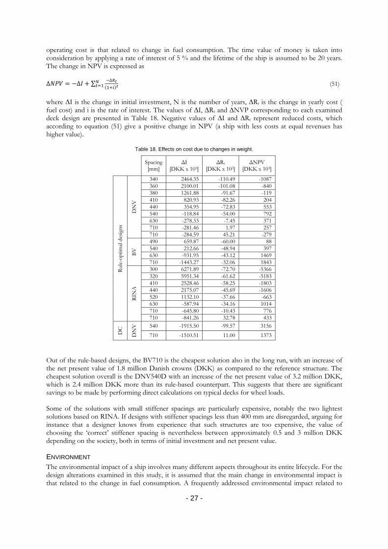
The relationship between S and displacement (M), as read from the hydrostatics calculations [18], is illustrated in Figure 18 and ΔS is approximated by linear interpolation as

∆𝑆 = ∆𝑀 ∙ 𝑆7.4−𝑆7.5𝑀7.4−𝑀7.5

(46)

- 24 -

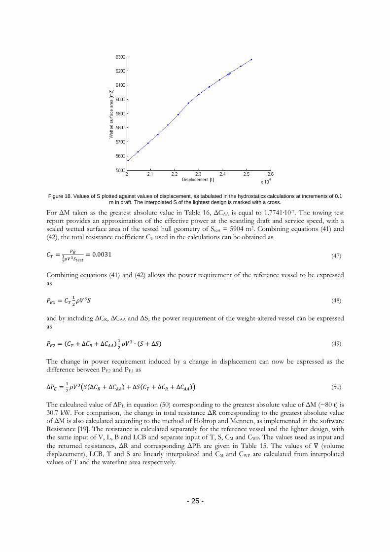
Figure 18. Values of S plotted against values of displacement, as tabulated in the hydrostatics calculations at increments of 0.1 m in draft. The interpolated S of the lightest design is marked with a cross.

For ΔM taken as the greatest absolute value in Table 16, ΔCAA is equal to 1.7741∙10-7. The towing test report provides an approximation of the effective power at the scantling draft and service speed, with a scaled wetted surface area of the tested hull geometry of Stest = 5904 m2. Combining equations (41) and (42), the total resistance coefficient CT used in the calculations can be obtained as

𝐶𝑇 = 𝑃𝐸12𝜌𝑉

3𝑆𝑡𝑒𝑠𝑡= 0.0031 (47)

Combining equations (41) and (42) allows the power requirement of the reference vessel to be expressed as

𝑃𝐸1 = 𝐶𝑇12𝜌𝑉3𝑆 (48)

and by including ΔCR, ΔCAA and ΔS, the power requirement of the weight-altered vessel can be expressed as

𝑃𝐸2 = (𝐶𝑇 + ∆𝐶𝑅 + ∆𝐶𝐴𝐴) 12𝜌𝑉3 ∙ (𝑆 + ∆𝑆) (49)

The change in power requirement induced by a change in displacement can now be expressed as the difference between PE2 and PE1 as

∆𝑃𝐸 = 12𝜌𝑉3�𝑆(∆𝐶𝑅 + ∆𝐶𝐴𝐴) + ∆𝑆(𝐶𝑇 + ∆𝐶𝑅 + ∆𝐶𝐴𝐴)� (50)

The calculated value of ∆PE in equation (50) corresponding to the greatest absolute value of ΔM (~80 t) is 30.7 kW. For comparison, the change in total resistance ΔR corresponding to the greatest absolute value of ΔM is also calculated according to the method of Holtrop and Mennen, as implemented in the software Resistance [19]. The resistance is calculated separately for the reference vessel and the lighter design, with the same input of V, L, B and LCB and separate input of T, S, CM and CWP. The values used as input and the returned resistances, ΔR and corresponding ΔPE are given in Table 15. The values of ∇ (volume displacement), LCB, T and S are linearly interpolated and CM and CWP are calculated from interpolated values of T and the waterline area respectively.

- 25 -

Table 15. Input and results of calculations according to Holtrop and Mennen.

Weight-independent input Weight-dependent input Results

ΔM [kg]

V [kt]

L [m]

B [m]

∇ [m3]

LCB [m]

T [m]

S [m2]

CM [-]

CWP [-]

R [kN]

ΔR [kN]

ΔPE [kW]

0 22.3 184.81 25.6 23635.3 86.265 7.5 6185.8 0.9566 0.8808 1465.66 4.86 55.7 -79841 23557.6 86.285 7.4818 6177.0 0.9565 0.8801 1460.80

There is a significant difference between the two approximations of the change of power requirement. There is some uncertainty associated with the interpolation of ΔCR in equation (44), but it is hardly expected to account for the entire difference. The changes in power requirement corresponding to the remaining rule-optimal designs and the two DC-improved designs are given in Table 16.

Table 16. Effects on performance due to changes in weight.

Spacing [mm]

ΔM [kg]

ΔGM [mm]

ΔS [m2]

ΔPE [kW]

Rule

-opt

imal

des

igns

DN

V

340 -79841 -4.99 -8.83 -30.7 360 -73039 -4.56 -8.07 -28.1 380 -66237 -4.13 -7.32 -25.5 410 -59435 -3.71 -6.57 -22.9 440 -52618 -3.28 -5.82 -20.2 540 -39014 -2.43 -4.31 -15 630 -5379 -0.33 -0.59 -2.1 710 1423 0.09 0.16 0.5 710 32649 2.02 3.61 12.6

BV

490 -43345 -2.70 -4.79 -16.7 540 -35355 -2.20 -3.91 -13.6 630 -31148 -1.94 -3.44 -12 710 -23158 -1.44 -2.56 -8.9

RIN

A

300 -52524 -3.27 -5.81 -20.2 320 -44518 -2.77 -4.92 -17.1 410 -42078 -2.62 -4.65 -16.2 440 -33009 -2.05 -3.65 -12.7 520 -27208 -1.69 -3.01 -10.5 630 -24675 -1.53 -2.73 -9.5 710 -7537 -0.47 -0.83 -2.9 710 23674 1.47 2.62 9.1

DC

DN

V 540 -71945 -4.49 -7.95 -27.7

710 7943 0.49 0.88 3.1

ECONOMY The change in fuel consumption is calculated by multiplying the change in effective power by the specific fuel consumption of the engine, here taken as 165 g/kWh for a typical MDO-engine. The input for the calculation of change in fuel cost is listed in Table 17.

Table 17. Input for fuel cost calculation

Yearly time at sea [h]

Specific fuel consumption [g/kWh]

Fuel price [USD/t]

Exchange rate [DKK/USD]

4056 165 930 [20] 5.78 [21]

For the assessment of the economic values of each of the deck designs in relation to the reference structure, the change in net present value (NPV) associated with the design is evaluated based on the changes in initial investment and yearly operating cost. The NPV can be used for assessing and comparing different long-term investments, since it considers the time value of money by reducing the values of future cash flows to their present worth with respect to interest. It is here assumed that the only change in

- 26 -

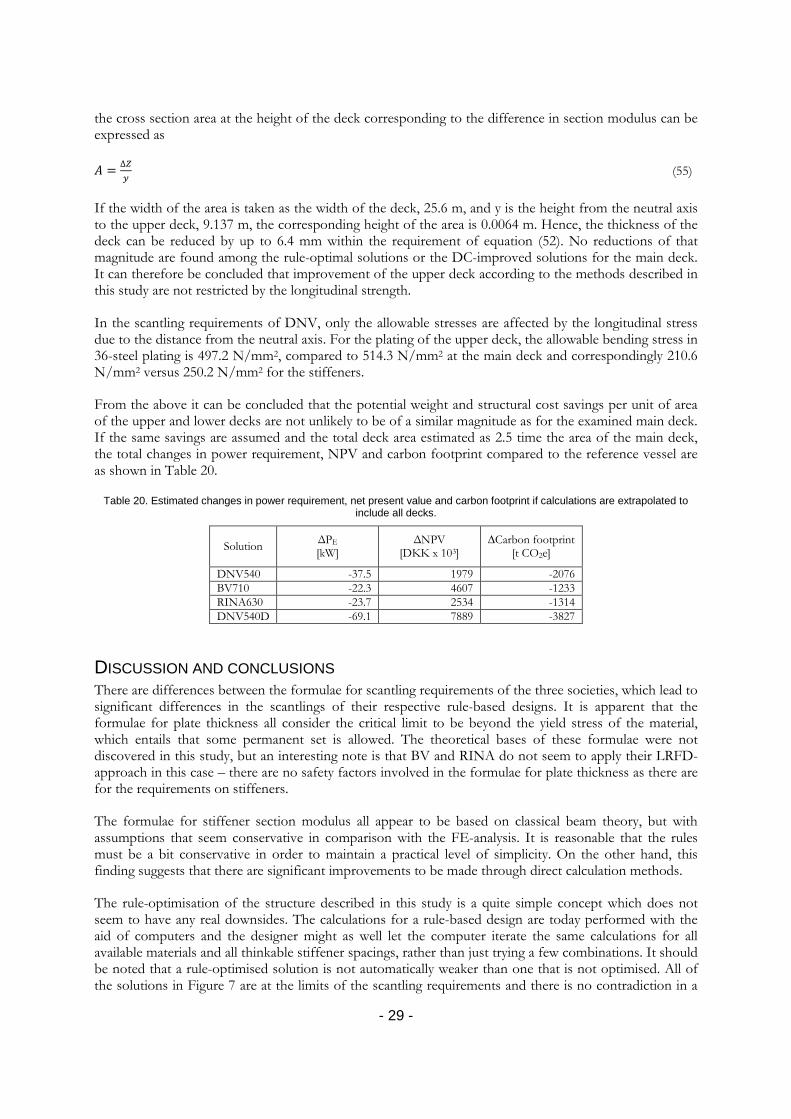
operating cost is that related to change in fuel consumption. The time value of money is taken into consideration by applying a rate of interest of 5 % and the lifetime of the ship is assumed to be 20 years. The change in NPV is expressed as

∆𝑁𝑃𝑉 = −∆𝐼 + ∑ −∆𝑅𝑡(1+𝑖)𝑡

𝑁𝑡=1 (51)

where ∆I is the change in initial investment, N is the number of years, ∆Rt is the change in yearly cost ( fuel cost) and i is the rate of interest. The values of ∆I, ∆Rt and ∆NVP corresponding to each examined deck design are presented in Table 18. Negative values of ∆I and ∆Rt represent reduced costs, which according to equation (51) give a positive change in NPV (a ship with less costs at equal revenues has higher value).

Table 18. Effects on cost due to changes in weight.

Spacing [mm]

ΔI [DKK x 103]

ΔRt [DKK x 103]

ΔNPV [DKK x 103]

Rule

-opt

imal

des

igns

DN

V

340 2464.35 -110.49 -1087 360 2100.01 -101.08 -840 380 1261.88 -91.67 -119 410 820.93 -82.26 204 440 354.95 -72.83 553 540 -118.84 -54.00 792 630 -278.33 -7.45 371 710 -281.46 1.97 257 710 -284.59 45.21 -279

BV

490 659.87 -60.00 88 540 212.66 -48.94 397 630 -931.95 -43.12 1469 710 -1443.27 -32.06 1843

RIN

A

300 6271.89 -72.70 -5366 320 5951.34 -61.62 -5183 410 2528.46 -58.25 -1803 440 2175.07 -45.69 -1606 520 1132.10 -37.66 -663 630 -587.94 -34.16 1014 710 -645.80 -10.43 776 710 -841.26 32.78 433

DC

DN

V 540 -1915.50 -99.57 3156

710 -1510.51 11.00 1373

Out of the rule-based designs, the BV710 is the cheapest solution also in the long run, with an increase of the net present value of 1.8 million Danish crowns (DKK) as compared to the reference structure. The cheapest solution overall is the DNV540D with an increase of the net present value of 3.2 million DKK, which is 2.4 million DKK more than its rule-based counterpart. This suggests that there are significant savings to be made by performing direct calculations on typical decks for wheel loads.

Some of the solutions with small stiffener spacings are particularly expensive, notably the two lightest solutions based on RINA. If designs with stiffener spacings less than 400 mm are disregarded, arguing for instance that a designer knows from experience that such structures are too expensive, the value of choosing the ‘correct’ stiffener spacing is nevertheless between approximately 0.5 and 3 million DKK depending on the society, both in terms of initial investment and net present value.

ENVIRONMENT The environmental impact of a ship involves many different aspects throughout its entire lifecycle. For the design alterations examined in this study, it is assumed that the main change in environmental impact is that related to the change in fuel consumption. A frequently addressed environmental impact related to

- 27 -

the combustion of fossil fuels is the global warming, caused by the emission of greenhouse gases into the atmosphere, and an emerging method of measuring that impact is called carbon footprinting. The basic concept of the method is to quantify all emissions of greenhouse gases caused by a product during its entire lifecycle and express the sum in weight units of C02-equivalents (CO2e). The British Standards Institution refers to this measure as “Life cycle GHG emissions” [22]. At the time of writing, the International Standards Organisation (ISO) does not have a standard for the calculation of carbon footprints, but has announced that “ISO 14067, Carbon footprint of products” is to be published in 2014 [23].

The UK government’s Department for Environment, Food and Rural Affairs (Defra) provides conversion factors for converting a quantity of MDO into kg CO2e. The C02-equivalents of the direct emission, from combustion of the fuel in the engines, is calculated using the factor 3527.6 kg CO2e/t [24]. The emissions associated with the fuel before it reaches the tank of the vessel, taking into consideration the extraction, transportation and refinement of the crude oil, are called indirect emissions and their C02 equivalents are calculated using the factor 607.6 kg CO2e/t [24]. The total change in carbon footprint is taken as the sum of the direct and indirect emissions. The values corresponding to the total (20-year) fuel savings of the solutions with highest NPV of each society are presented in Table 19.

Table 19. Change in carbon footprint induced by change in fuel consumption.

Solution

∆Fuel (20 years) [t]

∆Direct emissions [t CO2e]

∆Indirect emissions [t CO2e]

∆Carbon footprint [t CO2e]

DNV540 -201 -709 -122 -831 BV710 -119 -421 -72 -493 RINA630 -127 -448 -77 -526 DNV540D -370 -1307 -225 -1532

In order to put the values in Table 19 in some perspective, it might be helpful to compare them with carbon footprints of more tangible concepts. Two examples found in [25] are the carbon footprints of driving one mile at 60 mph in a small modern car, 350 g CO2e, and of deforestation of one hectare, 500 t CO2e. The difference in carbon footprint between the reference structure and DNV540D is thus equivalent to driving 7 million km or to deforestation of about 3 ha. It should be noted that [25] is popular literature and the calculations behind the carbon footprints are not presented.

GENERALISATION If the structure of the main deck can be improved as described in the previous chapters, it should be expected that also the remaining two decks can be improved to some extent, provided that their scantlings are determined by the same formulae. However, this might not be the case if the ship is limited by its longitudinal strength. In such a case, the required strength would most efficiently be attained by increasing the thickness of the upper deck, since this is the longitudinal material which is farthest from the neutral axis.

The hull girder section modulus at the height of the upper deck of the reference vessel is 11.312 m3 [26] and the rule requirement of DNV (the society by which the vessel is approved) is

𝑍𝑂 = |𝑀𝑆+𝑀𝑊|𝜎𝑙

∙ 103 = 9.809 ∙ 106 𝑐𝑚3 = 9.806 𝑚3 (52)

Recognising that the section modulus at height y from the neutral axis is expressed as

𝑍 = 𝐼𝑦 (53)

and that the moment of inertia of a thin horizontal plate at height y can be expressed as

𝐼 = 𝐴 ∙ 𝑦2 (54) - 28 -

the cross section area at the height of the deck corresponding to the difference in section modulus can be expressed as

𝐴 = ∆𝑍𝑦

(55)

If the width of the area is taken as the width of the deck, 25.6 m, and y is the height from the neutral axis to the upper deck, 9.137 m, the corresponding height of the area is 0.0064 m. Hence, the thickness of the deck can be reduced by up to 6.4 mm within the requirement of equation (52). No reductions of that magnitude are found among the rule-optimal solutions or the DC-improved solutions for the main deck. It can therefore be concluded that improvement of the upper deck according to the methods described in this study are not restricted by the longitudinal strength.

In the scantling requirements of DNV, only the allowable stresses are affected by the longitudinal stress due to the distance from the neutral axis. For the plating of the upper deck, the allowable bending stress in 36-steel plating is 497.2 N/mm2, compared to 514.3 N/mm2 at the main deck and correspondingly 210.6 N/mm2 versus 250.2 N/mm2 for the stiffeners.

From the above it can be concluded that the potential weight and structural cost savings per unit of area of the upper and lower decks are not unlikely to be of a similar magnitude as for the examined main deck. If the same savings are assumed and the total deck area estimated as 2.5 time the area of the main deck, the total changes in power requirement, NPV and carbon footprint compared to the reference vessel are as shown in Table 20.

Table 20. Estimated changes in power requirement, net present value and carbon footprint if calculations are extrapolated to include all decks.

Solution

ΔPE [kW]

ΔNPV [DKK x 103]

∆Carbon footprint [t CO2e]

DNV540 -37.5 1979 -2076 BV710 -22.3 4607 -1233 RINA630 -23.7 2534 -1314 DNV540D -69.1 7889 -3827

DISCUSSION AND CONCLUSIONS There are differences between the formulae for scantling requirements of the three societies, which lead to significant differences in the scantlings of their respective rule-based designs. It is apparent that the formulae for plate thickness all consider the critical limit to be beyond the yield stress of the material, which entails that some permanent set is allowed. The theoretical bases of these formulae were not discovered in this study, but an interesting note is that BV and RINA do not seem to apply their LRFD-approach in this case – there are no safety factors involved in the formulae for plate thickness as there are for the requirements on stiffeners.

The formulae for stiffener section modulus all appear to be based on classical beam theory, but with assumptions that seem conservative in comparison with the FE-analysis. It is reasonable that the rules must be a bit conservative in order to maintain a practical level of simplicity. On the other hand, this finding suggests that there are significant improvements to be made through direct calculation methods.

The rule-optimisation of the structure described in this study is a quite simple concept which does not seem to have any real downsides. The calculations for a rule-based design are today performed with the aid of computers and the designer might as well let the computer iterate the same calculations for all available materials and all thinkable stiffener spacings, rather than just trying a few combinations. It should be noted that a rule-optimised solution is not automatically weaker than one that is not optimised. All of the solutions in Figure 7 are at the limits of the scantling requirements and there is no contradiction in a

- 29 -

solution being heavy, expensive and weak at the same time, due to a disadvantageous combination of materials and stiffener spacing.

The FE-analyses in this study involve some uncertainties. Firstly, one might question the appropriateness of evaluating stresses that exceed the yield limit by a linear elastic model. It is not clear exactly how the maximum linear elastic stress is related to what happens after the yield point, in terms of e.g. an acceptable level of permanent set or the ultimate strength of the structure. Secondly, the analyses are performed for the loads which are determined to be most severe according to the rules (of DNV). There might therefore be a possibility that the examined loads are not the most severe out of all the possible configurations of the design loads on the deck. Regarding the plating, there is also the applicability of the model to consider - the flexibility of the stiffeners included in the model significantly reduces the stress along the edges of the plate, but in the case when one of the stiffeners is replaced by a longitudinal girder, the stress in the plating will be higher. However, the savings related reducing the scantlings of stiffeners are shown to be significant and it is also indicated that the rule formulae for stiffeners are conservative. It is therefore argued that the reduction of stiffener scantlings through direct calculations is worthwhile and should be examined in closer collaboration with the classification society when it is allowed.

The cost approximations used in this study are very rough, but they are only meant to be used for ranking the different solutions and to provide an idea of the order of magnitude of the potential savings. However, a more thorough investigation of the cost model for the structure might be motivated, because a more accurate model might return different result of the optimisation.

Benefits related to the lower fuel consumption of a lighter design are found to be significant, both in terms of economic savings and reduced environmental impact.

In conclusion, the rule-optimisation is a helpful tool for selecting good deck designs and design by direct calculation gives significant improvements if it is allowed by the classification society.

- 30 -

REFERENCES 1. Larsen, N.G., 2012. Senior Naval Architect at Knud E. Hansen A/S and supervisor of this study. (Personal communication).

2. Petromedia, 2012. Portworld. [Online] Available at: http://www.portworld.com/map/ [Accessed 24 November 2012].

3. Ship Structure Committee, 2007. Comparative Study of Ship Structure Design Standards. [Online] Available at: http://www.shipstructure.org/pdf/446.pdf [Accessed 28 June 2012].

4. Det Norske Veritas, 2012. Rules for Classification of Ships Pt 5 Ch 2: Passenger and Dry Cargo Ships. [Online] Available at: http://exchange.dnv.com/publishing/RulesShip/2012-07/ts502.pdf [Accessed 17 September 2012].

5. Det Norske Veritas, 2012. Rules for Classification of Ships Pt 3 Ch 1: Hull Structural Design, Ships with Length 100 metres and above. [Online] Available at: http://exchange.dnv.com/publishing/RulesShip/2012-07/ts301.pdf [Accessed 17 September 2012].

6. Bureau Veritas, 2012. Rules for the Classification of Steelships. [Online] Available at: http://erules.veristar.com/dy/app/ [Accessed 4 December 2012].

7. RINA, 2012. Rules for the Classification of Ships Part B: Hull and Stability. [Online] Available at: http://portal.rina.org/portal/server.pt/gateway/PTARGS_0_199956_2921_372_0_43/https%3B/webdomino.rina.org/RINA/QS-RINA/QSDCRINA.nsf/0/CC93E4DD876FFFB1C1257ADA003395B3/$file/REP2-ENG.ZIP [Accessed 4 December 2012].

8. Young, W.C. & Budynas, R.G., 2002. Roark’s Formulas for Stress and Strain. 7th ed. McGraw-Hill.

9. Björk, K. 2011. Formler och tabeller för mekanisk konstruktion. Karl Björks Förlag.

10. Caprani, C. 2008. Continuous Beam Analysis. [Online] Available at: http://www.colincaprani.com/files/programs/CBA.zip [Accessed 17 September 2012].

11. Corus Special Profiles, 2002. Bulb Flats. [Online] Available at: http://www.tatasteeleurope.com/file_source/StaticFiles/Business%20Units/Special%20Strip/Bulbflat.pdf [Accessed 17 September 2012].

12. Det Norske Veritas, 2012. Rules for Classification of Ships Pt 3 Ch 2: Hull Structural Design, Ships with Length less than 100 metres. [Online] Available at: http://exchange.dnv.com/publishing/RulesShip/2012-07/ts302.pdf [Accessed 17 September 2012].

13. Watson, D.G.M., 1998. Practical Ship Design. Elsevier.

14. Schneekluth, H. & Bertram, V., 1998. Ship Design for Efficiency and Economy. 2nd ed. Oxford: Butterworth-Heinemann.

15. Lyngstad, O.A., 2012. Principal Surveyor at DNV. [E-mail] (Personal Communication 8 November 2012).

16. Knud E. Hansen A/S, 2007. Loading condition for KEH06035.

17. SSPA Marine Consulting, 1999. KEH/STENA RoRo Vessel – Model Tests with Original Hull Form.

18. Knud E. Hansen A/S, 2007. Hydrostatic Values for KEH06035.

- 31 -

19. KTH Centre for Naval Architecture, n.d. Resistance. [Software].

20. Petromedia, 2012. Bunkerworld. [Online] Available at: http://www.bunkerworld.com/prices/ [Accessed 24 November 2012].

21. Saxo Bank, 2012. Valuta.se. [Online] Available at: http://www.valuta.se [Accessed 24 November 2012].

22. British Standard Institution, 2011. PAS 2050:2011 - Specification for the assessment of the life cycle greenhouse gas emissions of goods and services.

23. Hirner, H., 2012. Greenhouse gas emissions - ISO 14067 to enable worldwide comparability of carbon footprint data. ISO. [Online] Available at: http://www.iso.org/iso/home/news_index/news_archive/news.htm?refid=Ref1643 [Accessed 5 December 2012].

24. Defra, 2011. 2011 Guidelines to Defra / DECC's GHG Conversion Factors for Company Reporting. [Online] Available at: http://archive.defra.gov.uk/environment/business/reporting/pdf/110707-guidelines-ghg-conversion-factors.pdf [Accessed 5 December 2012].

25. Berners-Lee, M., 2010. How Bad Are Bananas?: The Carbon Footprint of Everything. Profile Books.

26. Knud E. Hansen A/S, 2007. Hull Section Scantlings according to DNV Rules/IACS CSR. (Calculations in Nauticus Hull, version 10.6.5730, rule edition July 2005).

- 32 -