ABSTRACT

BURKE, DAVID ALEXANDER. System Level Airworthiness Tool: A Comprehensive Approach to Small Unmanned Aircraft System Airworthiness. (Under the direction of Dr. Charles E. Hall Jr.).

One of the pillars of aviation safety is assuring sound engineering practices through

airworthiness certification. As Unmanned Aircraft Systems (UAS) grow in popularity, the

need for airworthiness standards and verification methods tailored for UAS becomes critical.

While airworthiness practices for large UAS may be similar to manned aircraft, it is clear that

small UAS require a paradigm shift from the airworthiness practices of manned aircraft.

Although small in comparison to manned aircraft these aircraft are not merely remote

controlled toys. Small UAS may be complex aircraft flying in the National Airspace System

(NAS) over populated areas for extended durations and beyond line of sight of the operators.

A comprehensive systems engineering framework for certifying small UAS at the system

level is needed. This work presents a point based tool that evaluates small UAS by

rewarding good engineering practices in design, analysis, and testing. The airworthiness

requirements scale with vehicle size and operational area, while allowing flexibility for new

technologies and unique configurations.

System Level Airworthiness Tool: A Comprehensive Approach to Small Unmanned Aircraft System Airworthiness

by David A. Burke

A dissertation submitted to the Graduate Faculty of North Carolina State University

in partial fulfillment of the requirements for the degree of

Doctor of Philosophy

Aerospace Engineering

Raleigh, North Carolina

January 22, 2010

APPROVED BY:

_______________________________ ______________________________ Dr. Charles E. Hall Jr. Dr. Stephen P. Cook Committee Chair ________________________________ ______________________________ Dr. Ashok Gopalarathnam Dr. Paul I. Ro

_____________________________ Dr. Nelson W. Couch

ii

DEDICATION

I would like to dedicate this dissertation to my parents Peggy and Steven Burke.

Without their love, understanding, and support over the last eleven years I never would have

made it this far.

iii

BIOGRAPHY

David Burke was born in Greenville, NC to Steven and Peggy Burke on Feb. 15th,

1981. He was always interested in computers and was greatly influenced by Blair Turner, a

retired Electrical Engineer who worked on one of the first computers, UNIVAC I. David

graduated from South Point High School in 1999 and entered North Carolina State

University in the fall of that same year. He triple majored in Computer Engineering,

Electrical Engineering, and Computer Science graduating in May of 2004 with all three

degrees. David began work on his Masters in Computer Engineering in the Fall of 2004

under the direction of Dr. Edward Grant in the Center for Robotics and Intelligent Machines

(CRIM) at NC State. His masters work focused on designing an omni-directional camera

system for the EvBot small mobile robot platforms used in the CRIM. David graduated with

his Masters in Computer Engineering in May 2007. In the Fall of 2007 he began work on his

Ph.D. in Aerospace Engineering under the direction of Dr. Charles E. Hall Jr. His Ph.D

research focused on developing a tool for evaluating small unmanned aircraft system

airworthiness funded by NAVAIR. David has been heavily involved in the Aerial Robotics

Club at NC State from 2001 until the present.

iv

ACKNOWLEDGMENTS

I would like to thank Dr. Hall and Dr. Cook for their continued guidance, advice, and

assistance during the last three years. Without their edits, advice, and many hours of working

through the difficult issues SLAT would never have come to fruition. I would like to thank

all of my friends for help keeping me sane and, in particular, Stearns Heinzen, Jason Bishop,

John Southwell, and Joe Moster for the help they have provided during the development of

SLAT. I would also like to thank NAVAIR and the 4.0P Navy Airworthiness Office for

sponsoring this research effort.

v

TABLE OF CONTENTS

Chapter 1: Introduction & Literature Review ......................................................................1

Chapter 2: Failure Modes, Effects, and Criticality Analysis (FMECA) ............................25

Chapter 3: Risk Model .......................................................................................................28

Chapter 4: Algorithm Development...................................................................................66

Chapter 5: Example Aircraft ..............................................................................................82

Chapter 6: Application of SLAT to Example Aircraft .......................................................91

Chapter 7: Summary & Conclusion .................................................................................120

References ........................................................................................................................124

Appendix A: Failure Counts and Base Point Calculations ..............................................128

Appendix B: Point Allocation for Example Tests ...........................................................134

Appendix C: Example Showing Units Error in CE Equation ..........................................164

Appendix D: Mapping from MIL-HDBK-516 to SLAT .................................................167

Appendix E: Operational Flight Tests .............................................................................186

vi

LIST OF TABLES

Table 1: UAV Classes for Ground Impact Analysis .........................................................24

Table 2: Failure Categories ...............................................................................................26

Table 3: Population Density Categories and Representative Values .................................39

Table 4: Example UAS Mission: Stadium Fly-Over .........................................................40

Table 5: Example UAS Mission: Perkins Field .................................................................42

Table 6: Example UAS Mission: Traffic Monitoring ........................................................43

Table 7: Phoenix Dimensions (Team 1, 2008-2009) .........................................................86

Table 8: Optikos Dimensions (Team 3, 2008-2009) .........................................................87

Table 9: Piolin Dimensions (Team 2, 2008-2009) ............................................................88

Table 10: Hyperion Dimensions (Team 1, 2005-2006) .....................................................89

Table 11: Goose Dimensions (Team 3, 2007-2008) ..........................................................90

Table 12: Example Change Log (Phoenix) ........................................................................95

Table 13: TLS Calculations ...............................................................................................97

Table 14: Failure Modes Addressed by FEA Test ...........................................................101

Table 15: Point Calculation for FEA Example (Structures Test 1) .................................102

Table 16: Wing Load Test Example Details ....................................................................105

Table 17: Compiled Flight Test Points for Optikos .........................................................106

Table 18: Full Example of SLAT – Structures Domain ..................................................113

Table 19: Full Example of SLAT – Propulsion Domain .................................................114

Table 20: Full Example of SLAT – Electrical Domain ...................................................114

vii

Table 21: Full Example of SLAT – Control System Domain .........................................115

Table 22: Full Example of SLAT – System Safety Domain ...........................................115

Table 23: Results Across All Domains for Initial Flight Tests ........................................117

viii

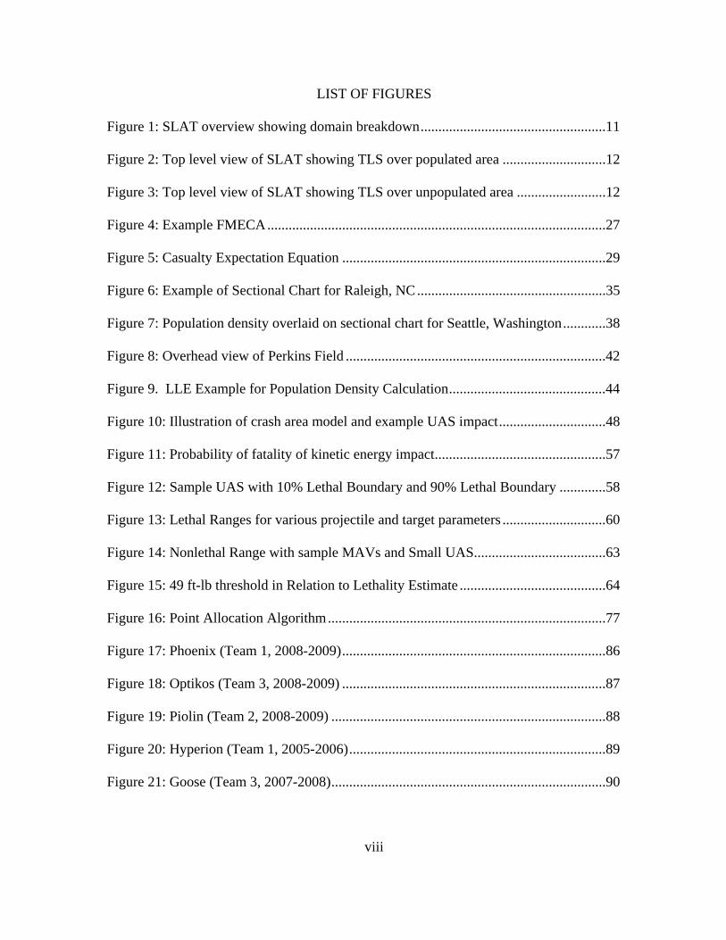
LIST OF FIGURES

Figure 1: SLAT overview showing domain breakdown ....................................................11

Figure 2: Top level view of SLAT showing TLS over populated area .............................12

Figure 3: Top level view of SLAT showing TLS over unpopulated area .........................12

Figure 4: Example FMECA ...............................................................................................27

Figure 5: Casualty Expectation Equation ..........................................................................29

Figure 6: Example of Sectional Chart for Raleigh, NC .....................................................35

Figure 7: Population density overlaid on sectional chart for Seattle, Washington ............38

Figure 8: Overhead view of Perkins Field .........................................................................42

Figure 9. LLE Example for Population Density Calculation ............................................44

Figure 10: Illustration of crash area model and example UAS impact ..............................48

Figure 11: Probability of fatality of kinetic energy impact ................................................57

Figure 12: Sample UAS with 10% Lethal Boundary and 90% Lethal Boundary .............58

Figure 13: Lethal Ranges for various projectile and target parameters .............................60

Figure 14: Nonlethal Range with sample MAVs and Small UAS .....................................63

Figure 15: 49 ft-lb threshold in Relation to Lethality Estimate .........................................64

Figure 16: Point Allocation Algorithm ..............................................................................77

Figure 17: Phoenix (Team 1, 2008-2009) ..........................................................................86

Figure 18: Optikos (Team 3, 2008-2009) ..........................................................................87

Figure 19: Piolin (Team 2, 2008-2009) .............................................................................88

Figure 20: Hyperion (Team 1, 2005-2006) ........................................................................89

Figure 21: Goose (Team 3, 2007-2008) .............................................................................90

ix

Figure 22: FEA Analysis Screenshot .................................................................................99

Figure 23: Physical Wing Load test of flight wing ..........................................................104

Figure 24: Autopilot Software FMECA Selection...........................................................109

Figure 25: SLAT Full Example, Optikos Prior to First Flight .........................................116

Figure 26: Opitkos SLAT after Initial Flight Tests .........................................................118

Figure 27: After Autopilot Added....................................................................................119

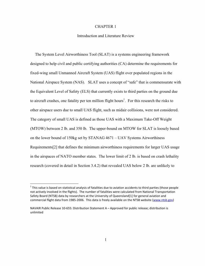
1

CHAPTER 1

Introduction and Literature Review

The System Level Airworthiness Tool (SLAT) is a systems engineering framework

designed to help civil and public certifying authorities (CA) determine the requirements for

fixed-wing small Unmanned Aircraft System (UAS) flight over populated regions in the

National Airspace System (NAS). SLAT uses a concept of “safe” that is commensurate with

the Equivalent Level of Safety (ELS) that currently exists to third parties on the ground due

to aircraft crashes, one fatality per ten million flight hours1. For this research the risks to

other airspace users due to small UAS flight, such as midair collisions, were not considered.

The category of small UAS is defined as those UAS with a Maximum Take-Off Weight

(MTOW) between 2 lb. and 350 lb. The upper-bound on MTOW for SLAT is loosely based

on the lower bound of 150kg set by STANAG 4671 – UAV Systems Airworthiness

Requirements[2] that defines the minimum airworthiness requirements for larger UAS usage

in the airspaces of NATO member states. The lower limit of 2 lb. is based on crash lethality

research (covered in detail in Section 3.4.2) that revealed UAS below 2 lb. are unlikely to

1 This value is based on statistical analysis of fatalities due to aviation accidents to third parties (those people not actively involved in the flights).  The number of fatalities were calculated from National Transportation Safety Board (NTSB) data by researchers at the University of Queensland[1] for general aviation and commercial flight data from 1985‐2006.  This data is freely available on the NTSB website (www.ntsb.gov)  NAVAIR Public Release 10‐655: Distribution Statement A – Approved for public release; distribution is unlimited   

2

cause life threatening injury in the event of an uncontrolled crash. SLAT limits its range to

below the vehicles covered by STANAG 4671 and above the 2 lb. nonlethal limit.

The airworthiness requirements – criteria, standards, and verification methods –

dictated by SLAT scale based on the population density of the mission area and the threat of

a vehicle crash to people on the ground. Methods for determining population density

categories for mission risk assessment, UAS crash lethality and an impact model have been

incorporated such that SLAT prescribes very few requirements for flights over unpopulated

areas to very stringent requirements for flight over open air assemblies. By bringing all of

the different UAS domains into a comprehensive framework, SLAT allows a CA or project

manager to easily determine a system's strengths and weaknesses, while also allowing CA to

compare levels of airworthiness among dissimilar UAS. It is expected that this tool could be

used by both project managers in industry and CA to determine the most cost effective

manner to design, build and test small UAS by providing them a clear path toward

certification with built-in flexibility for new technologies and techniques.

1.1 Airworthiness Summary

Before any discussion of UAS airworthiness can be undertaken it is important to

understand the airworthiness process for manned aircraft. Airworthiness is defined2 as the

ability of an aircraft to obtain, sustain, and terminate flight in accordance with prescribed

2 This is specifically the definition used by the U.S. military.  The civil authorities typically define airworthiness as the adherence to the aircraft Type Certificate and the standards required for such a certification. 

3

usage requirements [3]. This covers all phases of flight and focuses on the aircraft’s ability

to fly. Safety of Flight (SoF) is another term that is often used when discussing airworthiness

and is defined as the property of an air system configuration to safely attain, sustain, and

terminate flight within prescribed and accepted limits for injury/death to personnel and

damage to equipment, property and/or environment [3]. An example of a safety of flight

concern would be a non-flight critical component inadvertently falling off an aircraft (e.g. a

missile falls off a fighter jet during maneuvers). The loss of the missile would not present an

airworthiness concern since the aircraft would be able to continue flying without any

problems, but it would pose a danger to people on the ground. For UAS operations in the

NAS the focus has been primarily on the SoF restrictions (i.e. no flights over populated

areas) rather than evaluating the true airworthiness of the system.

For U.S. military aircraft the guidelines for airworthiness are defined in MIL-HDBK-

516B [3]. The US civil airworthiness standards are defined in the Federal Aviation

Regulations (FAR) contained in Title 14 of the Code of Federal Regulations (CFR) [4].

Subchapter C parts 21 through 49 contain detailed airworthiness and SoF requirements

separated by aircraft type, use, and some individual components3. The European Union (EU)

has very similar legislation for civil airworthiness covered in CS parts of the same numbers

(FAR Part 23, which defines U.S. airworthiness requirements for the small airplane category,

is basically mirrored by CS Part 23 for the EU). 3 The US civil airworthiness standards are designed such that engines and propellers are certified separate from the aircraft.  FAR Part 35 contains all of the airworthiness requirements for propellers.  This differs from the standard military approach of certifying the airworthiness of the aircraft as a whole (if the engine is changed the airworthiness release would need to be modified to reflect the configuration change).  SLAT follows the military model in its approach to configuration control.  

4

The fundamental difference between the military and civil airworthiness approaches

is the amount of flexibility. The military airworthiness process is designed to be very

flexible in order to accommodate large variation in aircraft designs and missions. A fighter

jet is so significantly different from a cargo aircraft that no single set of airworthiness

guidelines would be able to appropriately cover both contexts. MIL-HDBK-516B [3] defines

a set of guidelines for tailoring a large set of airworthiness criteria to match the aircraft

configuration being reviewed.

There are four key terms in regards to airworthiness tailoring; criterion, standard,

verification method, and artifact. The airworthiness criteria are very broad goals such as

“show that the aircraft structures are sufficiently strong,” but they don’t specify what

constitutes sufficiently strong or how to show that some sufficient threshold has been met.

Therefore a standard has to be associated with each criterion such as “all structures shall be

built with a 1.5 factor of safety between the limit and ultimate load4.” The third aspect is the

verification method, which is how the aircraft manufacturer is going to show that the

standard was met. For manned aviation the structures are often tested by loading the wings

until failure. This conclusively shows that the actual aircraft structures didn’t fail until at

least 150% of the limit load. The artifact is the deliverable or report that can be archived as

proof that the criterion, standard, and verification method were followed and achieved.

For military aircraft the appropriate CA goes through the process of developing an

Engineering/Data Requirements Agreement Plan (EDRAP). An EDRAP goes through the

4 The limit load in airworthiness is the highest load condition within the prescribed flight envelope.  The ultimate load is the point at which the structures fail. 

5

extensive lists of criteria in [3] to determine which criteria apply for this specific aircraft.

Once the criteria are chosen the appropriate standards and verification methods are chosen.

Finally the artifacts that are expected by the CA are defined such that the manufacturer is

clear as to the items they need to produce to get a flight clearance. By following this process

the EDRAP defines the requirements that the aircraft must meet to be considered airworthy,

which is typically called the airworthiness basis.

In many ways SLAT mimics the EDRAP approach. SLAT uses a system engineering

tool to tailoring the criteria, while providing a method for handling differing standards and

verification methods. The deliverables in SLAT that earn points are effectively the artifacts

required by the EDRAP process. Since SLAT has been designed to follow the military

airworthiness process it was important that all of the items in [3] were accounted for or

discussed in SLAT. Appendix D has a mapping from MIL-HDBK-516B [3] to the various

sections of SLAT. It contains discussion of any items that don’t map into SLAT and also

discusses those items in SLAT that have no parallel in [3].

The civil airworthiness processes are much more rigid than the tailored approach used

by the military. This occurs because civil aircraft typically follow very similar mission

profiles. They take off from one location, reach a cruising altitude, transit or loiter at that

altitude, and then land. This is true for small General Aviation (GA) aircraft was well as

commercial jetliners although the scale of the flight differs and certain aspects such as cabin

pressurization and oxygen apply for higher altitude flights. The civil standards are separated

by aircraft size and application to capture these differences. Effectively this tailors the

6

airworthiness requirements into just a handful of categories. Airworthiness certificates,

called Type Certificates, are granted to an aircraft design after it has shown compliance with

all of the airworthiness requirements as dictated by law. In this way the airworthiness

requirements wrap the criterion in with the standard, verification methods, and artifacts. This

leads to a slightly different definition of airworthiness in the civil context that civil aircraft

airworthiness can be defined as adhering to the requirements of type certification.

1.2 System Engineering

SLAT is designed using a common Systems Engineering (SE) tool known as a

Failure Modes, Effects, and Criticality Analysis (FMECA). As such it is important to discuss

what SE means in an airworthiness context and how the SE approach has been applied during

the development of SLAT. The International Council on System Engineering (INCOSE) has

defined a system as “an interacting combination of elements, viewed in relation to function”

[5]. In the airworthiness context the entire aircraft is viewed as a system. SE itself is

difficult to define precisely. INCOSE defines it as “the interdisciplinary approach and means

to enable the realization of successful systems.” Simon Ramo gave the following

description:

Systems engineering is a branch of engineering that concentrates on the design and application of the whole as distinct from the parts…looking at a problem in its entirety, taking into account all of the facets and all of the variables and relating the social to the technical aspects. [5]

The essence of SE is to approach any system, whether it is an aircraft or a manufacturing

facility, as a whole entity that is comprised of smaller pieces or subsystems. It allows

7

designers to view the big picture of the entire system and still be able to focus on the intimate

details of the individual components.

There are a number of system engineering tools that are commonly used in current

airworthiness processes. Functional Hazard Assessments (FHA) examines the effects of

various hazards on the entire system and is able to account for hazards that result from the

failure of a combination of functions [5]. Fault Tree Analysis (FTA) breaks the system down

hierarchically from subsystems down to individual components. FTA are useful in determine

the probability of a top level event such as Probability of Loss of Aircraft (PLOA) or

Probability of Loss of Control (PLOC). A disadvantage of FTA is that it requires significant

reliability information on the individual components in order to calculate a high confidence

in the top level event. There are methods for handling uncertainty in the base component

failure rates [6], but it can still be difficult to calculate the top level event with the confidence

needed for flights over populated areas. Other SE tools such as Common Cause Analysis

(CCA) or Event Trees can be used to determine failure paths and how failures in different

subsystems can have the same outcome. SLAT uses a FMECA to help define the different

failure modes and how those failures affect the overall system. Chapter 2 has a more in-

depth discussion of the FMECA process and how it is used in SLAT.

1.2.1 UAV vs. UAS

A UAS is defined as a remotely piloted, semi-autonomous, or autonomous air vehicle

and its operating system. These are systems that are designed to be recovered and reused and

as such weapons systems such as cruise missiles are not considered UAS [7]. The term UAS

8

encompasses the entire system from the air vehicle to the ground station to the various data

links. The terms Unmanned Aerial Vehicle (UAV) or Unmanned Aircraft (UA) are often

used to refer to the actual airframe, while the term “drone” is often used by the media to refer

to military UAS. The Air Force often refers to UAS as Remotely Piloted Aircraft (RPA) to

emphasize that humans are in control of the aircraft and that the UAS isn’t making any

decisions. The Office of the Secretary of Defense (OSD) provided a more detailed definition

of UAV in the Unmanned Systems Road Map 2005-2030[7] which states that an Unmanned

Aircraft is:

A powered, aerial vehicle that does not carry a human operator uses aerodynamic forces to provide vehicle lift, can fly autonomously or be piloted remotely, can be expendable or recoverable, and can carry a lethal or non-lethal payload. Ballistic or semi ballistic vehicles, cruise missiles, and artillery projectiles are not considered unmanned aerial vehicles.

These unmanned systems require a significant paradigm shift in terms of how airworthiness

and safety of flight are determined since there are no crew or passengers onboard the aircraft.

Most of the functions of the pilot are being performed autonomously and the operator on the

ground is dependent on the Command and Control (C2) link to maintain Situational

Awareness (SA) of the system's state, location, and any failures that may have occurred

onboard the vehicle.

The small UAS category covers such a broad range of vehicles that no single set of

airworthiness standards could ever hope to fully address all of the unique aspects of all of the

vehicle configurations. If a blanket set of airworthiness requirements were mandated for all

small UAS it is likely that either there would be some size below which it is simply not

9

profitable or feasible to develop UAS or the standards would be inadequate for the larger

vehicles. One of the primary features of SLAT is the concept that "flexibility can lead to safe

and cost effective UAS development", but that flexibility must be defined and maintained in

a solid framework. SLAT provides this framework and includes many options for tailoring

the tool to a CA or project manager’s application.

1.3 SLAT Overview

SLAT is a point based tool where UAS earn points toward airworthiness based on good

engineering practices. Points are earned as a UAS manufacturer shows design, testing, and

mitigation artifacts to support the proposed operation of their vehicle. The foundation of

SLAT is a tailored FMECA where all of the possible failure modes are detailed along with

their causal modes and methods to mitigate each failure. The FMECA is done at the

component level for all of the domains except for System Safety, which is a functional

FMECA. The FMECA is tailored to capture the configuration of each UAS. This research

provides a fairly extensive set of base FMECAs to help facilitate the tailoring process5. The

applicant earns more points towards certification by addressing the most critical failures as

identified by the FMECA. Unlike more rigid “pass/fail” requirements for airworthiness

artifacts in manned aviation, the artifacts in SLAT are graded such that the number of points

depends on the quality of the analysis/testing performed.

5 These basis FMECA sets are supplied in the Supplemental Document SLAT_FMECAs.pdf that should accompany this dissertation. 

10

In the basis FMECA sets SLAT divides a generic UAS into six domains: Structures,

Propulsion, Electrical, Control System, Ground Station, and System Safety. The Structures

domain includes all physical structural members, the skin of the aircraft, control surfaces and

components, hatches, and landing gear or launcher system if applicable. The Propulsion

domain comprises the engine or motor, propeller, fuel systems, and power generation as

applicable. The Electrical domain includes all of the wiring, connectors, and electronic

servos in the aircraft. The Control System domain is comprised of two parts: External Pilot

and Autopilot. The Ground Station domain includes all of the components used by the

operators including the data/communication/payload links as applicable to the vehicle

configuration. The System Safety domain captures those functional aspects of the aircraft

that have not been captured by the individual domains. Specifically the System Safety

domain focuses on the interfaces between domains and operational aspects such as UAS

hand-off between two different control stations or interfacing between the autopilot operator

and an external pilot. Figure 1 shows the domain breakdown as it has been arranged for the

base FMECA sets. Clearly there are some components that are mutually exclusive (such as

Electric Motors and Reciprocating Engine) or items that may not be present in all

configurations (such as Power Generation). The first step in SLAT is to tailor the FMECA

sets to accurately reflect the specific UAS configuration being examined. The overlapping

FMECA sets are supplied to provide a larger basis for a UAS designer to pull from for the

initial configuration. By providing a sufficiently complete set of basis FMECA sets to draw

from that the tailoring process SLAT should be more approachable by developers who may

11

not be intimately familiar with the FMECA process. The basis FMECA sets also help define

a format for the FMECA process such that anyone using the tool should have FMECA sets

that are arranged in the same manner.

 

Figure 1. SLAT overview showing domain breakdown

The UAS must earn enough points such that all of the domains reach a common Target

Level of Safety (TLS). The TLS is the goal that a UAS must reach to be considered safe to

fly that particular mission. Each of the different domains has its own column and the goal is

to earn points by showing good engineering practices to bring each domain to at least the

TLS line. This is based on the concept that any UAS is only as safe as its weakest critical

component. The TLS algorithm was designed to scale with the threat of the vehicle to those

people on the ground and as such it is a function of the wingspan of the aircraft, the weight of

the aircraft, and the population density of the mission area. The TLS was designed such that

a 350 lb. UAS flying over the most crowded, least sheltered situation will be required to

appro

view

popu

6 The Tfor thi

oximate the r

of the top le

lation area.

Figur

           

Figure 3.

TLS algorithm ris top end scen

requirement

evel break do

re 2. Top le(red c

Top level vipopulated a

requires that anario. 

s for small m

own of SLA

vel view of columns indi

iew of SLATareas or with

all failure mode

12

manned aircr

AT and how t

SLAT showicate domain

 

T showing hoh respect to a

es that could re

raft6. Figure

the TLS scal

wing TLS ovens below the

ow TLS chaa smaller UA

esult in the cra

es 2 and 3 be

les with the m

er populatedTLS)

 

anges over leAS

ash of the UAS 

elow shows a

mission

 

d area

ess

must be addre

a

essed 

13

1.3.1 Rationale for Pointed Based Tool

SLAT gains several advantages by being a point-based tool. First, the gains from

tests are quantifiable. A CA can examine a test and determine how much that test really

shows about the actual reliability of the system. Likewise, a program manager can look at

the possible number of points granted by several different tests and divide by the cost to

perform each test to get a solid metric on which test gives the most value. Second, the point-

based system allows dissimilar UAS to be compared against one another. This allows for the

CA to evaluate the relative safety strengths and weaknesses in different systems. Third, by

providing the tailored approach it is possible to reuse components/assembles/subsystems. A

company could easily have the same control system in several different UAS. If the Control

System FMECA set for all the aircraft are the same, then the points granted by any original

testing would also be the same. In this way a UAS developer could determine the relative

savings of equipment reuse and get credit for testing components in previous aircraft7. There

are two components in SLAT that are designed to leverage the experience of the CA offices.

The first component is known as Foundational Requirements and the second is the grading of

the tests by airworthiness experts.

7 There would, of course, still be failure modes inherent in those components that would still need to be addressed for this particular installation.  For example, even though an autopilot system onboard one UAS may have been tested for inference with other critical components that interference testing would still need to be repeated for a new aircraft since it is installation specific.  The manufacturer though wouldn’t have to repeat the reliability testing on the autopilot sensors since those haven’t changed. 

14

1.3.2 Foundational Requirements

The foundational requirements are mandatory items inacted by the CA to help cover

special situations or mandated by assumptions made during the design of the risk model. It is

impossible to design any tool as broad as SLAT and not have certain situations where the

tool could be abused, falls short of current safety practices, or simply doesn’t work well. The

foundational requirements are designed to allow such shortcomings to be addressed and

allow a CA to tailor SLAT to their use. SLAT has several base foundational requirements

that result from assumptions made during its design. First, SLAT is designed for fixed wing

aircraft only. It is likely that SLAT could be easily modified to include rotary aircraft, but

that would require in a change in the crash area model as the current model uses the UA

wingspan as the primary variable. Second, SLAT is designed for aircraft between 2 and 350

lb. MTOW. There are several assumptions made during the development of the risk model

(such as the effectiveness of hard and soft shelter) that are based on this size restriction. It

would be possible to reevaluate those assumptions to expand SLAT for a broader scope, but

in its current configuration it is limited to that size range. Another use of foundational

requirements is to capture those situations where the population density categories fit poorly

(see section 3.2 for more details on the population density categories). For example, consider

an exihibition of a UAS at a typically unpopulated flight test facility. This region may be

considered unpopulated for typical operations, but clearly inviting 500 people to come watch

a demonstration would violate the unpopulated status. Based on the population density

categories 500 people would not be enough to count as an open air assembly, but typically a

15

CA would consider such a gather so close to the operations area a high risk. A CA could

easily add a foundational requirement such as “any flight demonstration with more than 50

people in attendence for the specific purpose of viewing the UAS in flight shall be treated as

an open air assembly for purposes of calculating the TLS for that event.”

1.3.3Empowering CA Graders

The second item that leverages the experience in the CA offices is that SLAT

specifically empowers the experts in the airworthiness offices in the grading of tests. SLAT

provides a framework for acalculating how many points any particular test could be worth,

but the final step in awarding points is that an expert in that area grades the test. A grade of

100% would mean that the expert grader felt that those failure modes had been completely

examined by the artifact presented, while lesser grades reflect the proportion to which the

grader feels those failure modes have been addressed. Section 4.3.1 has a more indepth

discussion on the grading process.

16

1.4 History of Airworthiness

1.4.1 US Regulations and Agencies

Regulation of the aviation industry in the U.S. started in 1926 with the passage of the

Air Commerce Act. This piece of legislation placed civil aviation regulation under the

charge of the Secretary of Commerce and was pursued under the behest of the aviation

industry who believed that civil aviation would only be viable as long as there was some

federal oversight to mandate minimum safety standards [8]. The first airworthiness

certificates were issued in 1927 requiring aircraft manufacturers to show that they had meet

minimum engineering requirements and provide one aircraft for flight testing to receive an

airworthiness certificate [9]. At first this act created the Aeronautics Branch of the Dept. of

Commerce, but in 1934 this branch was renamed the Bureau of Air Commerce. This Bureau

focused on certification of pilots and aircraft, but also took over control of the three ATC

centers in 1936. In the 1938 the Civil Aeronautics Act created the Civil Aeronautics

Authority as a separate agency. This authority was split into two parts in 1940; the Civil

Aeronautics Administration (CAA) and the Civil Aeronautics Board (CAB). The CAA was

responsible for ATC, airmen and aircraft certification, safety enforcement, and airway

development. The CAB was entrusted with safety rulemaking, accident investigation, and

economic regulation of the airlines [8]. In the late 1940’s and early 1950’s airworthiness

standards were created to ensure continued safe flight and landing in the event of a failure of

key aircraft components. Also during this time the airworthiness requirements were

differentiated by the size of the aircraft. Small aircraft were defined as those with MTOW

17

below 12,500 lb. and the large aircraft category encompassed any large aircraft. These

definitions are still in use today [9].

In 1958 the CAA was replaced with the Federal Aviation Agency (FAA). This new

independent agency was the result of a public outcry after two separate midair collisions. In

1956 two commercial passenger aircraft collided above the Grand Canyon killing all 128

people on-board. In 1958 a fighter jet collided with a commercial passenger jet. Up until

this point the CAA was responsible for only civil aircraft making military flights outside of

their jurisdiction. The newly formed FAA was empowered with regulation over both civil

and military aircraft. In 1966 the independent agency was reformed as the Federal Aviation

Administration (FAA) as part of the newly formed Department of Transportation [8].

The FAA’s Aircraft Certification Service administers the type certification program

to determine compliance with the prescribed regulations and to maintain continued

airworthiness for all US aircraft [8]. The airworthiness regulations are defined in the Federal

Aviation Regulations (FARs), which are part of the Code of Federal Regulations (CFR). In

this way the airworthiness regulations in the US are a matter of law and therefore the FAA is

empowered to enforce those regulations with legal backing8. The FAA has numerous offices

each of which specializes in a specific type of certification. For example, the Small Airplane

Directorate is responsible for FAR 239, while the Rotorcraft Directorate is responsible for all

8 The FAA typically enforces these regulations through civil penalties, fines, or suspension of the offending party’s type certificate (which effectively prevents them from flying legally until the suspension is lifted).  Repeated violations have resulted in jail time for the offending party (typically pilots flying repeatedly without a license).   The FAA publishes its enforcement actions quarterly on their database, which is publically available at: http://www.faa.gov/about/office_org/headquarters_offices/agc/operations/agc300/reports/Quarters/ (cited 1 Feb. 2010).   9 FAR Part 23 covers the airworthiness requirements for most of the general aviation aircraft. 

18

the regulations related to helicopters and other rotorcraft. Each of the directorates is located

in a different region of the US. In this way the FAA groups the specialists and experts for

each field together to provide a solid knowledge base for their regulation activities.

1.4.2 European Regulations and Agencies

The regulation of civil aircraft in Europe is complicated by the fact that Europe is

comprised of numerous independent countries. Each country maintains its independence

although the formation of the European Union (EU) has allowed for regulations that carry the

weight of law to be applied in all of the member countries. Before 1970 each country was

responsible for its own aviation authority. Each authority would decide what it considered

safe and therefore aircraft from different countries in Europe were held to different standards.

In 1970 the Joint Aviation Authorities (JAA) was formed. The JAA is an associated body of

the European Civil Aviation Conference (ECAC) representing the civil aviation regulatory

authorities of a number of European states who have agreed to cooperate in developing and

implementing common safety regulatory standards and procedures [10]. The JAA develops

and maintains the Joint Aviation Requirements (JARs), which in many ways mimic the FARs

used in the US10. In Europe the ATC functions are managed by EUROCONTROL, which is

a separate intergovernmental organization. One of the major differences between the FAA

and JAA is that because the JAA is comprised of numerous independent aviation authorities

their decisions don’t carry the weight of law. The JAA is limited to making suggestions, 10 The JARs are so close to the FARs that most of the numbering is the same.  This makes is much easier to compare the two regulatory requirements.  There are certain minor differences in the airworthiness processes, but the FAA and JAA have a reciprocal agreement to honor each other’s type certificates when European aircraft are flying in US airspace and when US aircraft are flying in European airspace. 

19

which must be adopted by the individual countries in order for them to be enforceable. In

2002 the EU decided to transfer all airworthiness certification tasks from the national

aviation authorities to the European Aviation Safety Agency (EASA). By doing such the

airworthiness regulations and EASA were given the power of law across all member states of

the EU. The handover of responsibilities took several years, but the JAA system was closed

on 30 June 2009 although some aspects of the JAA Training Organization (TO) still exist

[10].

1.4.3 International Regulations

Europe and the US have the oldest history of airworthiness regulation, but those

regulations don’t apply to the rest of the world. The International Civil Aviation

Organization (ICAO) was formed in 1944 by the Convention on International Civil Aviation

[11] and is headquartered in Montreal, Canada. ICAO produces aviation standards and best

practices for distribution internationally. ICOA helps coordinate with the various national

authorities such as the FAA and EASA to promote safe and economically viable international

aviation. ICAO also works through the United Nations (UN) to help developing countries

establish safe aviation practices.

20

1.5 Literature Review

1.5.1 Existing Airworthiness Documents for Unmanned Systems

There are a number of documents that have been published as the first attempts at

defining airworthiness processes for UAS. NATO produced STANAG 4671– UAV Systems

Airworthiness Requirements [2] in 2009 to define the minimum airworthiness requirements

for UAS between 150 kg and 20,000 kg. These requirements were drawn directly from a

tailoring of CS 23/25[12] with the addition of some requirements on ground station

information display.

The European Aviation Safety Agency (EASA) published “Policy Statement:

Airworthiness Certification of Unmanned Aircraft Systems (UAS) “[13] in 2009 to outline

the EU process for UAS airworthiness certification. This policy makes several important

statements:

With no persons onboard the aircraft, the airworthiness objective is primarily targeted at the protection of people and property on the ground. A civil UAS must not increase the risk to people or property on the ground compared with manned aircraft of equivalent category.

Airworthiness standards should be set to be no less demanding than those currently applied to comparable manned aircraft nor should they penalise UAS by requiring compliance with higher standards simply because technology permits.

The EASA policy focuses on tailoring the manned aviation standards for UAS

although it allows applicants to proposed UAS specific standards if they so choose. This

policy does not provide any standards itself, but it does provide a kinetic energy (KE)

approach to determine which of the manned aircraft categories a UAS most likely

resembles. More details about this KE approach are discussed in section 3.5 as part of the

21

risk modeling done for SLAT. The EASA airworthiness policy has no specific limits on

aircraft size, but since it is primarily focused on applying the manned aircraft airworthiness

standards it is most likely geared toward UAS larger than the 350 lb. upper limit of this

research.

The Federal Aviation Administration (FAA) has created the AFS-407 Unmanned

Aircraft Program Office to specifically handle the aspects of integrating UAS into the

National Airspace System (NAS). In 2008 the AIR-160 office has defined an Interim

Operational Approval Guidance document that defines the current UAS certification process

[14]. This document defines UAS airworthiness as follows: “for the UAS to be considered

airworthy, both the aircraft and all of the other associated support equipment of the UAS

must be in a condition for safe operation. If any element of the systems is not in condition

for safe operation, then the UA would not be considered airworthy.” This policy also

attempts to tailor the manned aviation standards for UAS. Of primary concern of the FAA

is the chance of a midair collision between a UAS and a manned aircraft due to the UAS

being unable to “see and avoid” other air traffic. Due to this concern the majority of the

certification process focuses on filling in this gap with ground based visual observers or

chase aircraft.

The FAA released “Small Unmanned Aircraft System Aviation Rulemaking

Committee, Comprehensive Set of Recommendations for sUAS Regulatory Development”

[15] in April of 2009. This set of proposed rulemaking defines small UAS as below 55 lb.

MTOW. The primary focus of this proposed rule making is to define operational categories

22

rather than specific airworthiness requirements. Of interest in this proposed rulemaking is

that it specifically includes hobby remote control (RC) aircraft as one of its operational

categories. Most of the discussion in the proposed rulemaking involves operational limits,

such as remaining under 400 feet AGL and within visual range of the operator, rather than

specific airworthiness standards.

1.5.2 UAS Integration Plans

Along with the work done in defining UAV reliability the OSD has also published the

“UAS Integration Roadmap” [7] in 2005 that outlines the military’s plan for integrating UAS

into its force structure. This report is focused on the high level goals rather than specifically

tackling the airworthiness concerns, but one of the primary recommendations made in the

report is “Foster the development of policies, standards, and procedures that enable safe,

timely, routine access by UA to controlled and uncontrolled airspace.”

1.5.3 MIT International Center of Air Transportation (ICAT)

MIT ICAT has done significant research into commercial air transport safety since

the late 1980’s [16]. Of primary relevance to this work is a report produced in 2005 titled

“Safety Considerations for Operation of Unmanned Aerial Vehicles in the National Airspace

System” [17]11. This substantial document outlines many of the difficulties in integrating

UAS into the NAS. It covers two key areas of UAS integration; Midair collisions and

Ground Impact. The midair collision component is beyond the scope of this research, but the

11 This ICAT report is effectively the same document as Roland E. Weibel’s master’s thesis of the same title[30]. 

23

ground impact research is relevant enough to discuss in more detail. [17] uses the terms ELS

and TLS in basically the same context as they are used in SLAT. The ground fatality rate

that is used in [17] is 5x10-7 rather than 1x10-7 fatalities per flight hour used in SLAT, but

this is a relatively small difference and is likely due to including fatalities to second parties

(e.g. ground crew, spectators, etc.) in the fatality rate calculation.

There are several key differences between the scope of work in [17] and SLAT. First,

[17] examines the entire range of UAS from 2.16 oz to 25,600 lb. whereas SLAT is strictly

limited to those UAS below 350 lb. Second, [17] combines shelter factor and crash lethality

into a single variable Ppen (probability of penetration). It does state the assumption that if

debris penetrates shelter then a fatality has occurred. From the report it is unclear how this

variable is actually derived and the results of Ppen seem questionable. The report fails to

provide the actual equation and states only that:

The probability of penetration, Ppen, depends on many factors, including the energy of the vehicle, the amount of energy several structures can withstand, and the distribution of people within those structures. For this general approach, a single factor estimate of probability of penetration was used. The probability of penetration shown in Table 11 was estimated based on kinetic energy of the aircraft in cruise, and the realization that the factor will vary from 0% to 100% from low to high energy impacts. –pg. 69 of [17]

Table 1 below is a reprint of Table 11 from [17] (pg. 69 of [17]). It shows the Ppen value in

the right-most column and the crash area in the next column to the left.

24

Table 1. UAV Classes for Ground Impact Analysis. Originally Table 11 in [17].

  It seems quite questionable that a 0.14 lb aircraft has a 5% chance of causing a fatality,

especially after shelter factor has been taken into account. It also seems odd that a 25,000 lb.

aircraft only has a 90% chance of penetrating a building during an uncontrolled crash.

Without the equation being provided it seems that those numbers were chosen based on some

expert opinion. It is unfortunate that such an exhaustive analysis of the state of UAS

integration into the NAS failed to cite any of the base equations for some of the most

promising research. The third area where there are significant differences is in the impact

model. [17] uses a crash area model that is roughly equivalent to the planform of the aircraft.

Section 3.5.1 has a more in-depth discussion of the crash area model used in SLAT, but it

was felt that the model used in [17] underestimated the area affected by a crashing UAS in

most scenarios.

25

CHAPTER 2

Failure Modes, Effects, and Criticality Analysis (FMECA)

SLAT uses tailored FMECA sets as the foundation for the tool. A FMECA is a system

safety tool that provides a framework for breaking down a complex system to into

subsystems, then assemblies, and finally down to its base components. At the component

level all the reasonable failure modes are explored. An attempt is made to determine what

causal factors could lead to each failure mode, what the result of the failure will be to that

domain and the overall system, and how bad that failure is in comparison to other failures.

One of the final results from a FMECA is a list of recommendations on how to avoid each

failure mode on an individual causal mode basis12. These recommendations provide valuable

data that the CA wants to see during the airworthiness certification process.

To be able to characterize the severity of the failure, it is helpful to create failure

categories. SLAT uses a four failure categories: Catastrophic, Critical, Major, and Minor.

These hazard categories are based on the format typically used by the military and FAA for

hazard analysis. A Catastrophic failure is the most feared event of an uncontrolled crash of

the UAS or fatality to the ground crew. During the initial FMECA research it was found that

there were series of failures that dictated the creation of a subcategory of the Catastrophic

category called Catastrophic Fly-Away. This subcategory of Catastrophic captures those

12 The FMECA format often has a column for recommended actions [29] that can help avoid a particular failure mode.  It is the entries from that column that is discussed as the final result of the FMECA that relates to the test creation in SLAT. 

26

failures that result in an unmanned aircraft flying without supervision and with no way of

recovering that supervision. The Fly-away failure category, although not totally unique to

unmanned systems, is much more of concern with the human crew removed from the

aircraft13. The Critical failure category captures those failures that result in an inability to

maintain flight, but where some control over the aircraft trajectory is still maintained (i.e.

loss of propulsion, aircraft can still glide away from populated areas). The Major and Minor

categories capture those failures that result in some reduction in safety margins, but are not a

direct threat to the aircraft. Table 2 below shows the basic descriptions for each of the failure

categories and their priority.

Table 2: Failure Categories Hazard Level Description Ref

#

Catastrophic Complete loss of control of the aircraft or fatality to ground crew. The vehicle has had a failure where the crew cannot control where it crashes.

1

Catastrophic Fly-away

The aircraft has gone “dumb” and is flying out of the mission area under some form of autopilot control with the operator unable to redirect the vehicle.

1

Critical

Loss of operator control over aircraft, inability to maintain flight trajectory or injury to ground crew. This includes lost link situations where the autopilot goes to a predetermined rally location as well as loss of propulsion where the crew still has control over the vehicle, but can no longer maintain altitude.

2

Major

Emergency situation, land as soon as practicable. This includes failures that significantly reduce safety margins or vehicle performance or significantly increase ground crew work load.

3

13 The situation where the pilot falls asleep or is incapacitated on a manned aircraft would be equivalent to the catastrophic fly‐away failure in SLAT. 

27

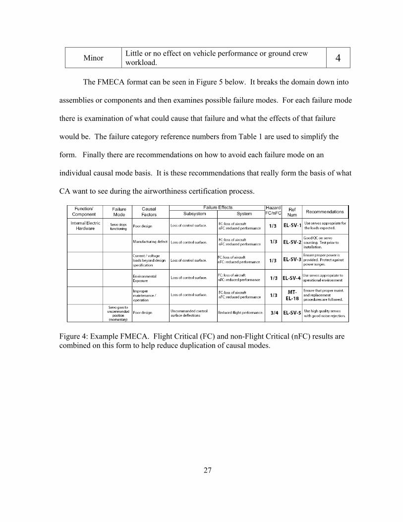
Minor Little or no effect on vehicle performance or ground crew workload. 4

The FMECA format can be seen in Figure 5 below. It breaks the domain down into

assemblies or components and then examines possible failure modes. For each failure mode

there is examination of what could cause that failure and what the effects of that failure

would be. The failure category reference numbers from Table 1 are used to simplify the

form. Finally there are recommendations on how to avoid each failure mode on an

individual causal mode basis. It is these recommendations that really form the basis of what

CA want to see during the airworthiness certification process.

 

Figure 4: Example FMECA. Flight Critical (FC) and non-Flight Critical (nFC) results are combined on this form to help reduce duplication of causal modes.

28

29

CHAPTER 3

Risk Model

The TLS is designed to scale with the threat of the vehicle to people in the operation

area. In order to accomplish this scaling a risk model was developed to encapsulate the

relative threat that any small UAS poses to people on the ground. There are three

components to the risk model used in SLAT. First, there is method for easily calculating an

exposed population density in the mission area. Second, an impact model has been

developed to represent how large of an area is affected by a UA crash and, third, a crash

lethality model has been investigated to determine the probability of someone within the

crash area sustaining a life threatening injury. These three components allow for risk

comparisons between dissimilar UAS and are used directly in the calculation of the TLS.

3.1 RCC-323-99 Casualty Expectation (CE) Equation

The Range Commanders Council (RCC) has previously attempted to create a risk

model for UAS operations on closed test ranges. The RCC has produced a standard, RCC-

323-99 "Range Safety Criteria for Unmanned Air Vehicles [18], for UAS flights at military

ranges. In the "Rationale and Methodology Supplement" to the RCC-323-99 standard

Appendix D contains a CE equation for calculating expected number of casualties per flight

hour. The equation as defined in RCC-323-99 is shown in figure 5 below.

30

CE = PF * PD * AL * PK * S Where: CE = Casualty Expectation (fatalities per flight hour) PF = Probability of Failure per flight hour (dimensionless) PD = Population Density (people per square mile) PK = Probability of Fatality (dimensionless) AL = Lethal Area (square feet) S = Shelter Factor (dimensionless) 

Figure 5: Casualty Expectation Equation [18]

The equation defined in Figure 5 was one of the principal starting points for the initial

concept of SLAT and is directly used later in the development of the Target Level of Safety

within SLAT. The equation has a very logical approach to risk modeling built up from first

principles, but unfortunately it can be very difficult to implement. In many ways the CE

equation over simplifies the problem of trying to calculate the actual risk posed by a UAS. It

works well in very controlled environments, such as the military test ranges that it was

designed for, where the different variables can be determined to a high degree of certainty,

but as uncertainty arises in the variables it accumulates to the point that the final risk

assessment could be in question.

The first difficulty is with the definition of PF or the probability of a catastrophic

failure per flight hour. This value can be difficult to quantify with any confidence for aircraft

using well known components. In the small UAS arena this value becomes nearly

impossible to determine to a high level of confidence as the component level failure rates for

many UAS assemblies are simply unknown. Many small UAS are using hobby grade

components that have never been subjected to a rigorous reliability study and in many cases

31

have very few quality control measures on their manufacturing (at least when compared to

those measures held by manufacturers of manned aircraft components). Also, one of the

great advantages of small UAS is their reduced cost. If every manufacturer had to perform

the reliability studies needed to quantify their component failure rates to a high degree of

confidence then the cost of these small UAS could exceed their usefulness. Therefore, the

PF variable can be estimated, but since it is multiplied in this equation the confidence values

of the final casualty estimation can only be as good as the confidence in this probability

estimate. SLAT specifically tries to avoid requiring calculation of the system level failure

rates as the confidence in these estimates is likely to be in question.

Another problem exists in determining the Shelter Factor variable S. Shelter factor is

defined as “an estimate of how exposed a population is to a vehicle or debris that may be

falling. A shelter factor of 1 assumes that the entire population is exposed, and a shelter

factor of 0 assumes that the entire population is completely sheltered [18]”. The shelter

factor for controlled environments can be fairly easily determined, but it is extremely

difficult to determine the shelter on a much broader basis (such as across the entire NAS). A

large number of assumptions would need to be made in order to determine the average

shelter factor of the population of the United States. These assumptions would likely

introduce significant uncertainty and variance that propagates through the entire CE equation.

The end result is that the CE equation can be dominated by the assumptions made in the

determination of the shelter factor variable. Shelter Factor could be assumed to be 1 across

the entire NAS, but this would likely push the equation toward being very conservative (after

32

all even a car is significant shelter from a 3 lb. aircraft). The concept of shelter factor isn’t a

flaw, but rather it is attempting to quantify shelter factor on some grand scale that could

undermine the usefulness of that part of the CE equation. SLAT uses the concept of shelter

factor in its population density calculations discussed in the next section of this report and in

the calculation of the Target Level of Safety, but avoids trying to quantify the S variable

directly.

Another issue to be aware of is that the CE equation as it is written in Appendix D of

[18] can be very prone to error due to an assumption of unit conversion for the PD

(population density) and AL (lethal area) calculations. The PD variable is the average

population density of the mission profile in units of “people per square mile”, while the AL

variable is the impact area model for the aircraft in units of “square feet.” Unfortunately, the

units on these two variables don’t match so it is an error to multiply them together directly.

A correction factor of 3.59 x 10-8 can be added to the equation to make the units work out

properly14. This error has a tendency for users to calculate PF values that are overly

conservative by a factor of magnitude roughly 28 million. Appendix C contains an example

of how this units error can occur and how the equation behaves once the correct conversion

factor is explicitly stated.

It is important to note that the CE equation was never developed for broad use across

the NAS. Rather, it was designed specifically for risk assessment on controlled military test

ranges and some of its assumptions were based on those people at risk being first or second 14 There are 27,878,400 square feet in a square mile.  The inverse of this value yields the 3.59 x 10-8 correction factor to convert population density into people per square foot rather than people per square mile. 

33

parties to the activities. Applying this equation to the entire NAS where the focus is

primarily on third parties would likely take it out of scope from its initial design. Also the

compounding reduction in confidence of the other variables due to limited equipment and

funding as is found in many small UAS further makes directly applying the CE equation to

the entire NAS difficult. The CE equation presented in [18] works well when all of the

variables can be determined with a high degree of certainty, but once large scale assumptions

begin to be made the confidence in the equation degrades quickly. The CE equation though

did provide some useful components for SLAT’s design, especially in the PK (probability of

kill) variable and discussion of the difficulties in the PD variable.

3.2 Shelter Factor

Since SLAT limits its scope to those UAS less than 350 lb. there are certain

assumptions that can be made about the shelter factor. Logically, there are numerous

structures (e.g. concrete buildings) that will provide basically complete protection from even

the largest of the UA in the small UAS category. For this research this type of shelter will be

referred to as hard shelter. Also, logically, there are many types of shelter (such as being

inside a car) that may provide significant protection from a UA that weighs 5 lb., but would

provide less protection as the size of the aircraft increases. This type of shelter will be

referred to as soft shelter. SLAT handles these two aspects of shelter in different parts of the

risk model. Hard shelter is used as part of the supporting argument for the Population

Density research presented in Section 3.3, while soft shelter is incorporated as part of the

derivation of the TLS algorithm in Section 4.1.

34

3.3 Population Density

As the population density increases the requirements demanded by SLAT increase

significantly. Flight over an open air assembly demands the strictest requirements, while the

requirements for flying in unpopulated areas remains low enough to allow for initial flight

testing of new systems. Using population density as a requirement can be difficult due to

different sources of population density data being available and discretization problems due

to different sampling sizes. If population density is going to be used to draw a “line in the

sky” (i.e. some UAS is not safe enough to fly over population densities greater than 500

people per square mile), such as was done with NASA's Ikhana UAS flights [19] in 2007,

then the line needs to be the same regardless of what data is being used or how that data is

being partitioned. Ideally there exists a single source for this data that is updated regularly,

easy to access, and will not be open to interpretation.

3.3.1 Population Categories vs. Continuous Function

Using national census data to determine population density has its difficulties. The

census is taken only every 10 years so the data will likely be inaccurate to the true population

density of the area. Different approaches for estimating growth between census years exist

and some communities may have published more recent population data. More importantly,

the census data is averaged over different sized areas called census blocks. If a sampling of a

population is taken at different resolutions (sampling every square mile versus sampling

35

every city block) then the results will be different and the line where the population density

crosses some threshold will change based on what sampling pattern is used. Therefore, using

this method the line in the sky would be dependent not only on the data itself, but also how

that census data is partitioned. This dependency on the data sampling is a form of

discretization error and any approach that treats population density as a continuous function

will suffer from these types of errors.

One approach to minimize these errors is to establish some very broad population

density categories. Current operational standards make reference to several broad categories

such as Densely Populated, Sparsely Populated, and Open Air Assembly. The term Open Air

Assembly is defined by the FAA [20] as any gathering of more than 1000 people at an

outdoor event. The term for Sparsely Populated is defined by the Department of Commerce

[21] as 500 people per square mile. The remaining terms are not defined by some direct

population density metric, but rather they are based on a qualitative assessment of the local

area by the pilot of a manned aircraft. The sectional charts provided for Visual Flight Rules

(VFR) flights by National Aeronautical Charting Office (NACO) have areas highlighted

yellow to indicate cities and towns, which are typically referenced as being densely

populated. NACO uses aerial photos to draw these boundaries based on observable urban

development and although these regions are not directly derived from population density it is

logical that the population density should be higher in regions of increased observable urban

development.

36

 

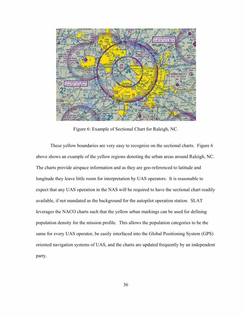
Figure 6: Example of Sectional Chart for Raleigh, NC.

These yellow boundaries are very easy to recognize on the sectional charts. Figure 6

above shows an example of the yellow regions denoting the urban areas around Raleigh, NC.

The charts provide airspace information and as they are geo-referenced to latitude and

longitude they leave little room for interpretation by UAS operators. It is reasonable to

expect that any UAS operation in the NAS will be required to have the sectional chart readily

available, if not mandated as the background for the autopilot operation station. SLAT

leverages the NACO charts such that the yellow urban markings can be used for defining

population density for the mission profile. This allows the population categories to be the

same for every UAS operator, be easily interfaced into the Global Positioning System (GPS)

oriented navigation systems of UAS, and the charts are updated frequently by an independent

party.

37

SLAT defines four separate broad population density categories: unpopulated, sparsely

populated, densely populated, and open air assembly. Any area inside the yellow regions on

the sectional chart are considered densely populated, while sparsely populated will be any

region outside of the yellow area not already defined as unpopulated or an open air assembly.

Unpopulated areas are regions where it is reasonable to expect that no persons or very few

persons other than the UAS operations crew, such as over the open ocean or within

controlled test ranges. The unpopulated category is primarily designed as a classification for

specific flight test ranges and facilities where UAS flight tests can be conducted in a

controlled environment. It is expected that the certifying authority would maintain a list of

accepted unpopulated areas for flight tests and that UAS companies could apply for such

classification at their facilities at which time they would have to show that the area is indeed

unpopulated and have their control procedures reviewed by the certifying authority.

3.3.2 Average Population Values and Shelter Factor

Clearly the actual population density in the yellow boundaries will vary significantly

from city to city. The largest urban areas in the US have population densities above 50,000

people per square mile, while many small towns have population densities closer to 1000

people per square mile. In both cases the cities would be marked as yellow “observable

urban areas.” Obviously a factor of 50 in the population densities between the two extremes

can’t be simply ignored, but a simplification can be made due to the size of the aircraft in

38

question. SLAT is being specifically developed for UA less than 350 lb. and the only way to

get population densities like those found in very large urban areas is to vertically stack

people in rather durable buildings. The vast majority of persons in large urban areas are

inside buildings that would provide significant shelter from even the heaviest UA in the small

UAS category (this is the hard shelter discussed earlier). If an UA were to strike one of these

buildings it might threaten the people on one floor or just inside one of the windows of the

building, but no 350 lb. vehicle is going to be able to puncture through multiple stories to

threaten everyone in that building. This would suggest that even though the actual

population densities of large are huge, the number of people that are actually exposed at any

one time to a small UAS crash is rather small. This research proposes that as urban

population density increases the amount of shelter increases proportionally. The number of

people in an urban area that are actually threatened by an uncontrolled crash of a small UAS

will stay relatively constant regardless of the actual population density of the area due to a

proportional increase in hard shelter. This allows SLAT to treat all of the yellow urban

regions on the sectional charts as having the same exposed population rather than them

having the same population densities. To be conservative on this assumption the exposed

population has been based on the average population of urban areas (those under the yellow

boundaries) across a statistically large sampling of regions across the United States.

39

3.4 Population Density Results

The sectional maps for the continental US were pulled into a Geographic Information

System (GIS) program called ArcGIS. Using several of the tools inside ArcGIS the

boundaries of the urban areas were extracted and imported into a file format that ArcGIS can

use for queries. The raw 2000 Census data was also incorporated into ArcGIS allowing the

population data to be overlaid with the NACO Sectional Maps. From this the trends of

population density as a function of the distance from the yellow boundaries can be

determined. Figure 6 below shows an overlay of the raw population data from the 2000

census over the sectional map for the Seattle, WA area. Each black dot in Figure 7

represents 100 people. This initial run showed satisfactory qualitative correlation between

the population density and the regions of observable development.

 

Figure 7: Population density overlaid on sectional chart for Seattle, Washington region. Each black dot is 100 people (2000 Census Data).

40

The results of the GIS study showed that the average population density inside the

yellow regions was approximately 9,800 people per square mile. It was decided to take the

extreme categories one order of magnitude in each direction. This represents the lack of

shelter in the Open Air Assembly situation and that even in unpopulated test facilities the

ground crew is still endangered. Table 3 below show the population density categories and

their representative values.

Table 3: Population Density Categories and Representative Values Category People per square mile

Open Air Assembly 98,000 Densely Populated 9,800 Sparsely Populated 500

Unpopulated 50

3.5 Creating Missions

This population density method allows the operators to define a mission profile based

on the weighted average of the time spent in over each region. The time weighted average

approach was chosen to emphasis that the exposure interval is a major factor in risk

assessment. An aircraft that is flying over an open air assembly of people all day long is

much higher risk than an aircraft that does a two minute fly-over. In aviation safety the focus

is on fatalities per flight hour and as such the time weighted average captures the exposure

interval aspect of a flight that has several different exposure contexts.

For demonstration, an example mission profile was created for a small UAS called

Stadium Fly-Over. In this hypothetical mission a small UAS launches from a sparsely

populated area, transit into a densely populated area, does a fly-over of a football game,

41

loiters outside the football game for a while, and then transits back to the sparsely populated

region for landing and recovery. Table 4 below shows how to calculate the mission

population density for this mission given some example exposure times.

Table 4: Example UAS Mission: Stadium Fly-Over

Mission Stage

Population Category

Total Time Spent

% of Mission

Time Weighted Average

Population Density

Launch Sparsely Populated 0.25 hrs 5% 25

Ingress Densely Populated 0.75 hrs 15% 1470

Fly Over Open Air Assembly 0.08 hrs 1.6% 1584

Loiter Densely Populated 2.92 hrs 58.4% 5723 Egress Densely Populated 0.75 hrs 15% 1470

Landing Sparsely Populated 0.25 hrs 5% 25

Totals: 5 hrs 100% 10,297

In the case of the example shown in Table 4 the population density for this mission

would be 10,297 people per square mile. This Stadium Fly-Over mission will be used later

in the TLS algorithm and example application of SLAT.

As a contrast to the Fly-Over mission let’s look at two missions at a controlled flight

test facility. NCSU aerospace program has such a facility in Butner, NC called Perkins Field.

Perkins Field is located on the grounds of the NCSU Butner Beef Cattle Field Laboratory. It

is bordered on all sides by either pasture land or forests and requires passing through several

locked gates to access the 454 foot long runway. The runway was installed to provide a safe

and controlled facility for flight testing of the senior design aircraft and other research

42

projects. Since this facility is well controlled, it qualifies as Unpopulated as there are no

Beef Cattle Facility staff within the defined flight area. The flight box is a series of large

pastures which can be observed from the flight line. Since it is designed for Line of Sight

(LOS) operations all flights will be maintained within the Unpopulated region. At the end of

the spring semester the MAE department hosts a picnic at Perkins Field where all of the

aerospace engineering seniors and their parents are invited to see flight demonstrations of the

aircraft designed over the last two semesters. Each aircraft is safety qualified for picnic

flights by performing several successful flights in the controlled setting. Since the observers

are near the flight line for the picnic flights those days would not count as Unpopulated.

Instead they would count as Sparsely Populated since the total attendance is well below the

1000 people needed to qualify as an Open Air Assembly and it is outside of the yellow

boundaries on the sectional map15. Figure 8 below shows an overhead shot of the controlled

facility.

15 The CA could create the Foundational Requirement discussed earlier that any gathering of more than 50 people for such a flight demonstration be considered an Open Air Assembly for terms of the TLS calculation, but for this example it will treated as Sparsely Populated. 

43

 

Figure 8: Overhead view of Perkins Field with flight area denoted in red (left).

Table 5 below shows the calculation of a simple flight at Perkins Field in the

controlled setting and in the picnic setting. All of these flights are under R/C control with

altitudes below 400 feet. These missions will be used again during the discussion of the TLS

algorithm.

Table 5: Example UAS Missions: Perkins Field

Setting Population Category

Total Time Spent

% of Mission

Time Weighted Average Population Density

Picnic Flight Sparsely Populated 1.5 hrs 100% 500

Controlled Facility Unpopulated 1.5 hrs 100% 50

As another example let’s examine a UAS mission to monitor traffic in a large city. In this

mission the UAS launches from a sparsely populated area, ingresses and loiters over a

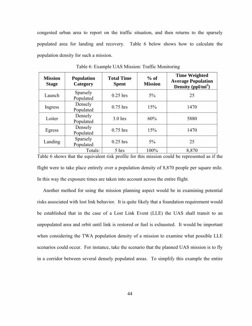
44

congested urban area to report on the traffic situation, and then returns to the sparsely

populated area for landing and recovery. Table 6 below shows how to calculate the

population density for such a mission.

Table 6: Example UAS Mission: Traffic Monitoring

Mission Stage

Population Category

Total Time Spent

% of Mission

Time Weighted Average Population

Density (ppl/mi2)

Launch Sparsely Populated 0.25 hrs 5% 25

Ingress Densely Populated 0.75 hrs 15% 1470

Loiter Densely Populated 3.0 hrs 60% 5880

Egress Densely Populated 0.75 hrs 15% 1470

Landing Sparsely Populated 0.25 hrs 5% 25

Totals: 5 hrs 100% 8,870 Table 6 shows that the equivalent risk profile for this mission could be represented as if the

flight were to take place entirely over a population density of 8,870 people per square mile.

In this way the exposure times are taken into account across the entire flight.

Another method for using the mission planning aspect would be in examining potential

risks associated with lost link behavior. It is quite likely that a foundation requirement would

be established that in the case of a Lost Link Event (LLE) the UAS shall transit to an

unpopulated area and orbit until link is restored or fuel is exhausted. It would be important

when considering the TWA population density of a mission to examine what possible LLE

scenarios could occur. For instance, take the scenario that the planned UAS mission is to fly

in a corridor between several densely populated areas. To simplify this example the entire

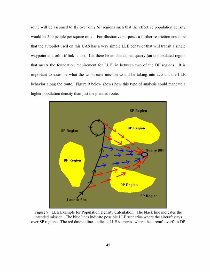
45

route will be assumed to fly over only SP regions such that the effective population density

would be 500 people per square mile. For illustrative purposes a further restriction could be

that the autopilot used on this UAS has a very simple LLE behavior that will transit a single

waypoint and orbit if link is lost. Let there be an abandoned quarry (an unpopulated region

that meets the foundation requirement for LLE) in between two of the DP regions. It is

important to examine what the worst case mission would be taking into account the LLE

behavior along the route. Figure 9 below shows how this type of analysis could mandate a

higher population density than just the planned route.

Figure 9. LLE Example for Population Density Calculation. The black line indicates the intended mission. The blue lines indicate possible LLE scenarios where the aircraft stays

over SP regions. The red dashed lines indicate LLE scenarios where the aircraft overflies DP

46

regions.

Figure 9 shows how the LLE could easily result in a mission with a significantly higher

effective population density. It is recommended in the use of SLAT that all possible LLE

scenarios be examined and that the highest population density value from all scenarios be

used as the population density for that mission.

3.6 Impact Model

Quantifying the threat that a UAS poses to people on the ground is a complicated

problem because there are numerous different ways that a UAS could crash. Having the main

wing spar buckle under load will likely result in a very different descent profile than if the

propulsion systems fails and the vehicle is in a gliding descent. To even further complicate

this problem there are many failures, such as loss of autopilot, that could result in a crash

profile that is somewhere in between a gliding descent and a plummeting crash. The

European Aviation Safety Agency (EASA) defined two different crash modes,

Unpremeditated Descent and Loss of Control, in "Policy Statement Airworthiness

Certification of Unmanned Aircraft Systems (UAS)"[13], which defines the European policy

on UAS airworthiness as of 2009. The Loss of Control crash mode corresponds to the

catastrophic failure in SLAT where the aircraft falls out of the sky with the operators unable

to modify its trajectory. This would include failures such as the main spar buckling under

load, failure of all flight control systems, loss of a flight critical control surface, etc. The

Unpremeditated Descent crash mode, on the other hand, encompasses those situations where

47

the aircraft cannot maintain flight, but where the operators still have some control over the

trajectory of the vehicle. This mode would include situations where the propulsion system

has failed or where a failure has resulted in such a reduction of safety margins that it is more

acceptable to purposefully crash the vehicle in some known safe location rather than risk

transit over heavily populated areas. This research has focused on the threat of a crashing

vehicle rather than operational aspects that could lead to a crash or midair collision. Due to

this separation the topic of Sense and Avoid is left to the regulatory agencies.

Logically, the threat of a UA to the people on the ground is related to how big of an

area the UA affects during a crash and how much energy is imparted into that area during the

crash. This breaks the vehicle threat problem into two parts: the crash area model and the

crash lethality model. The crash area model represents how large of an area is likely to be

affected by an UA crash, while the crash lethality models how likely a person is to sustain

life threatening injuries if they were struck by debris from a crashing UA.

3.6.1 Crash Area Model

Several different impact models have been proposed by different safety and certifying

groups. RCC-323-99 [18] has, as part of the CE equation discussed previously; two

approaches for modeling the crash area are presented. The first method uses the frontal area

of the vehicle as this corresponds to a vehicle crashing in a near vertical dive. This method

though is not particularly conservative as the chance of a vehicle maintaining a vertical dive

is not a likely type of failure. The more conservative approach presented in RCC-323-99

48

models the crash area as a rectangle swept by the wings as the aircraft descends along its

most efficient glide slope from 6 feet to impact with the ground. This “swept path” model

tends to be overly conservative as it is reasonable to assume that the mostly likely crash

trajectory will be something in between these two extremes.

For SLAT it was decided to focus on an impact model that exists somewhere in

between the Uncontrolled Descent type and the Swept Path type scenarios. It is expected that

with the loss of propulsion scenario that the operators in the ground station still have some

control over the aircraft and would be able to direct the vehicle to a safe area for a crash16. In

this way the “swept path” model is not the failure profile of significant concern. Several

different models were examined to try to find one that split the difference. RCC-321-07,

“Common Risk Criteria Standards for National Test Ranges” [22], has detailed methods for

determining the affected area in the case of a missile failure. This approach is very thorough,

but requires significant simulation17 to appropriately model. Since SLAT is trying to

determine a generic impact model that is independent of the exact flight area it was

determined that the approach presented in [22] would be over cumbersome or that to make it

useful the real value of that method would be lost in numerous assumptions. The SLAT

designers examined other methods of impact modeling and found an FAA Advisory Circular

16 Exactly what qualifies as a safe area for an emergency crash of the vehicle is beyond the scope of this research as it is an operations aspect of UAS integration into the NAS.  It is assumed that the flight plan for any UAS operation will be required to have certain specified areas for emergency crashes of the aircraft.  It will be up to the CA to determine the how those locations should be determined and how many should be in a specific flight plan.  The FAA has already required such crash locations in the flight planning of the Ikhana flights [20] and it is assumed that that requirement will likely become mandatory for UAS flights. 17 Typically a Monte Carlo type simulation of vehicle break up and debris dispersal is used in this type of analysis.  

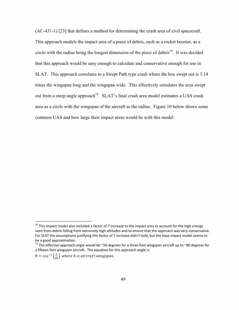
49

(AC-431-1) [23] that defines a method for determining the crash area of civil spacecraft.

This approach models the impact area of a piece of debris, such as a rocket booster, as a

circle with the radius being the longest dimension of the piece of debris18. It was decided

that this approach would be easy enough to calculate and conservative enough for use in

SLAT. This approach correlates to a Swept Path type crash where the box swept out is 3.14

times the wingspan long and the wingspan wide. This effectively simulates the area swept

out from a steep angle approach19. SLAT’s final crash area model estimates a UAS crash

area as a circle with the wingspan of the aircraft as the radius. Figure 10 below shows some

common UAS and how large their impact areas would be with this model.

18 This impact model also included a factor of 7 increase to the impact area to account for the high energy seen from debris falling from extremely high altitudes and to ensure that the approach was very conservative.  For SLAT the assumptions justifying this factor of 7 increase didn’t hold, but the base impact model seems to be a good approximation. 19 The effective approach angle would be ~50 degrees for a three foot wingspan aircraft up to ~80 degrees for a fifteen foot wingspan aircraft.  The equation for this approach angle is: 

. 

50

Figure 10: Illustration of Crash Area (left) and Example Crash Area with Sample UAS (right).

51

3.6.2 Crash Lethality

UAS pose a unique challenge for regulatory agencies in regards to airworthiness

certification. The lack of on-board crew or passengers dictates that the main concern during

a UAS crash is it striking people on the ground. A significant unknown is the likelihood of

someone dying if they are struck by a UAS. For large UAS it is very likely that anyone hit

would sustain life threatening injuries, but that may not be the case as the size of the aircraft

and its impact velocity are reduced. Logically at some point a UAS will be light enough and

moving slowly enough that it will be incapable of causing serious injury or death.

High vs. Low Fidelity Models

When modeling anything as complex as the interaction of a crashing vehicle and the

human body there are many different ways the problem could be approached. A high fidelity

model is one that tries to simulate the interactions as accurately as possible. This type of

model would have to take into account all the possible ways that an UAS could strike a

human (wing strikes body, wing strikes face, fuselage striking back of the head, etc.), the

shape of the impact area (i.e. how pointed the fuselage is or how sharp the leading edge of

the wing is), the presence of a propeller (pusher vs. tractor configurations and how the

propeller might cause lacerations), the way the vehicle is expected to break apart on impact,

the amount of kinetic energy the vehicle is likely to impart to the human body, and even if

there is the possibility of further injury due to fuel being ignited or exposure to other

hazardous substances. An in-depth overview of this type of modeling can be found in the

Range Commanders Council (RCC) Standard 321-07 "Common Risk Criteria Standards for

52

National Test Ranges: Supplement" [22]. This standard was written to address the numerous

dangers present at military test ranges, such as that of a missile breaking up after launch and

how debris falling back to the ground could harm civilians living nearby. RCC 321-07

incorporates much of the work done by the Risk and Lethality Commonality Team (RALCT)

and provides significant guidance on risk assessment across a wide range of applications.

The purpose of RCC 321-07 is to provide “a common set of range safety policies, risk

criteria, and guidelines for managing risks to people and assets during manned and unmanned

operations, excluding aviation operations” [22]. Many of the models discussed in RCC 321-

07 involve detailed Monte Carlo simulations to get the probability density functions to

describe how debris will be spread after an impact. Such simulations are quite time

consuming and require a significant amount of information on the various modes the vehicle

could be in as it approaches the impact site. Section 7.6.1 of [22] details the various Human

Vulnerability Models that could be used. Below is an excerpt from that report describing the

aspects of such a model:

Model Description. This model addresses human casualties that result from impact by inert (non-explosive) fragments. This includes (a) direct impact by a vehicle fragment, including impact by the fragment after it penetrates a structure, (b) impact by secondary debris created due to fragment splatter or cratering of the impacted surface, (c) secondary debris thrown out from an exploding fragment, or (d) impact by the secondary debris created by fragment penetration of, or blast damage to, a structure. Casualties from inert debris result from one or more of several injury mechanisms: • Penetration of the body by small, compact, high speed fragments. Since this generally requires high velocities it is not expected to result from impacting launch vehicle debris since, except for very early flight times,

53

the fragment velocities are not sufficiently high. It may result, however, from secondary debris from an exploding fragment or from secondary debris created by explosion loads acting on a structure. Penetration can be segmented into chunky penetration and piercing penetration. • Laceration or penetration by ragged metal fragments and glass shards by energy transferred to body organs and tearing of body tissues. • Blunt trauma resulting from the acceleration of body organs or excessive body deflections. Blunt trauma includes localized blunt trauma from small fragments that can impact over critical organs thus producing greater injuries. • Crushing resulting from heavy fragments pinning body segments between the fragment and a rigid object such as the ground or a wall.

• Fragment impact causing a person to fall and strike the ground/floor, wall or other object.

Such a detailed examination of how people could be injured would be useful for very specific

cases where the risk level needs to be determined with a high degree of confidence, but this

high fidelity modeling is so time consuming and has so many unknowns that it would be very

difficult to apply to the wide range of small UAS configurations and mission profiles. Also,

since SLAT uses a generalized approach to defining the vehicle characteristics and mission

locations an extreme number of assumptions would need to be made in order to run a high

fidelity model. Having that many assumptions would dramatically undermine the usefulness

of such a model and raise questions as to why so many resources were being allocated to

such a simulation.

Low fidelity models can be used to simplify the interaction between the human and

the UAS as they impact. The easiest way to do this simplification is to discuss how much

Kinetic Energy (KE) the impacting object has and how likely a human is to be injured based

54

on studies of KE transfer. This approach ignores how sharp the components are and how

debris might be thrown during an impact. The greatest advantage of this approach is that it is

very easy and fast to determine the KE of the impacting vehicle. RCC 321 also deals with

these types of models as shown in the excerpt below:

Historical models for human vulnerability to debris impact have been relatively simple models that predict casualty as a function of the fragment impact kinetic energy. These have often been expressed in terms of a single kinetic energy level above which a person is assumed to be a casualty. Common values that have been used range from about 11 foot-pounds for the casualty threshold to 58 foot-pounds for assured casualty.

This KE approach seems the most viable method for determining the possible

lethality of a small UAS since it is easy to apply in the design stage and can be applied to the

vast range of configurations.

Kinetic Energy The kinetic energy equation: makes calculating the kinetic energy of a

UAS at the moment of impact appear to be fairly straightforward. Unfortunately, the mass of

the UAS can vary between configurations and during a flight as fuel is burned off. More

importantly, the impact velocity can vary dramatically as potential energy is converted into

kinetic energy during the descent. Since velocity is squared in the KE equation even small

variations in velocity could result in significantly different lethality ratings. Solid definitions

for what will be used for both the UAS mass and impact velocity must be determined before

any kinetic energy approach will be viable.

55

Resolving the UAS mass to use can be determined by stating that SLAT will always

use the maximum take-off weight of the vehicle. This is a worst case approach since the

UAS may be flying at lower weights for the majority of its missions, but it is best to treat the

UAS at its most energetic configuration.

Determining the vehicle's crash velocity requires a bit more work. A UAS that is

crashing due to a complete loss of control is likely to have a much higher impact velocity

than one that has lost its engine and is gliding to the ground in a controlled manner. To deal

with these two conditions it is important to understand how they are approached in SLAT. In

the SLAT framework there are two types of failures likely to lead to crashes. The

Catastrophic failure can lead to an uncontrolled loss of the airplane, while the Critical failure

can lead to a controlled descent of the aircraft. Catastrophic failures are such events as loss

of a flight critical control surface, an on-board fire, or major structural failure; whereas the

Critical failures are such events as loss of propulsion, or other failures that render the aircraft

unable to safely maintain flight. In the case of Catastrophic failures it is expected that the

aircraft will crash immediately, while with critical failures the operators should have enough

control to aim the aircraft away from populated areas and allow it to crash in some

predetermined safe location. Since the operators should be able to ensure a relatively safe

crash landing of the UAS in the case of a Critical failure the main concern becomes the case

of a Catastrophic failure. The best approach for modeling crash lethality in SLAT is to have

it tied to the immediate uncontrolled crash of a UAS since that is the mode that is most likely

56

to result in the vehicle striking a person on the ground. The question then becomes how one

determines the average velocity of a vehicle crashing in an uncontrolled manor. It is

extremely unlikely that the vehicle would be able to convert all of its potential energy into

kinetic energy during such a descent, but it is very likely that some of that potential energy

transfer would occur. The designers of SLAT also want the lethality rating for a UAS to be

independent of the current altitude of the vehicle so that mission profile won't change the

lethality of the vehicle. For these reasons it is assumed that the potential energy transferred

to kinetic energy will occur within the first hundred feet or so of the descent. Thus the

vehicle would reach its impact velocity so quickly that the impact speed will be the same if it

were flying at 5,000 feet or at 200 feet.

The European Aviation Safety Agency (EASA) had similar thoughts on the subject

and published them in their "Policy Statement Airworthiness Certification of Unmanned

Aircraft Systems (UAS)" [13]. This policy contained two approaches for evaluating the

potential danger of UAS to civil populations. One of the approaches detailed in [13] involves

breaking the crash modes of UAS into two categories: Unpremeditated Descent and Loss of

Control. The Unpremeditated Descent scenario corresponds very nicely to the Critical

failure scenario in SLAT and the Loss of Control scenario corresponds to the catastrophic

failure scenario. They also discuss using the maximum take-off weight for the mass in the

kinetic energy calculation. For the Unpremeditated Descent scenario the impact velocity was

chosen to be 1.3 times the stall speed, while for the Loss of Control scenario it was chosen to

be 1.4 times the maximum operational speed. Since SLAT assumes that in the case of an

57

Unpremeditated Descent scenario the operators will be able to keep the vehicle away from

people then for this research the focus can be on just the Loss of Control scenario. The

EASA report doesn't officially define the maximum operating speed so this research assumes

it to be the speed of the UAS in level flight at sea level with 100% throttle. This velocity

data can be difficult to come by so all speeds will be referenced to the values given by the

manufactures and published in “UAS – The Global Perspective 2007/2008” [24] as the

maximum speeds for each system. .

Unfortunately, the assumption that a UAS will crash at 1.4 times its max operating

speed isn't based on any historical data. Rather it is a value defined in a

JAA/EUROCONTROL UAV Task Force Final Report [25] that states:

In the maximum impact speed scenario, the factor of 1.4 has been added based on existing regulatory requirements for manned aircraft flutter prevention. Above this speed, it could be expected that the UAV would structurally fail and break-up.

It is unclear whether the flutter onset for manned aircraft actually correlates to the flutter

onset for UAS. Making such an assumption would be difficult to support without UAS

flutter onset data. For the purposes of this report the factor of 1.4 times the max operating

speed will be considered an extremely conservative estimate of impact speed and as such will

be referred to as the worst-case scenario. The best case scenario would involve the aircraft

striking the ground with an impact velocity very close to its stall speed. This best-case

scenario would represent that an UAS converted none of its potential energy into kinetic

energy in the case of a loss of control event. As it is very unlikely that this would ever occur

this best-case scenario sets a reasonable lower limit on the possible kinetic energy range,

58

while the worst-case scenario of 1.4 times the maximum operating speed sets a reasonable

upper limit. For the rest of this report the UAS will be discussed based on their maximum

operating speeds. These velocities should be significantly above the speed of the UAS at the

onset of the failure, thus representing a kinetic energy increase. The worst-case scenario is

also easy to reference off the maximum operating speed by simply multiplying the speed by

1.4.

There are two previous attempts at categorizing lethality based on kinetic energy that

have been researched by the U.S. military. The Range Commanders Council has published a

UAS standard that includes a Casualty Expectation equation where lethality is fairly well

defined with regards to vehicle KE and several Army Research Lab technical reports have

used KE as the determining factor for less-than-lethal ammunitions.

Kinetic Energy Approach #1

The first approach is to examine only the kinetic energy of the vehicle without

regards to its relative size to the target or the area of interaction. A more in-depth view of

this approach can be found in RCC 323-99 "Range Safety Criteria for Unmanned Air

Vehicles: Rationale and Methodology Supplement" [18]. In Appendix D of RCC-323 the

following figure is provided as a smooth function for lethality probability for blunt trauma

against an average adult.

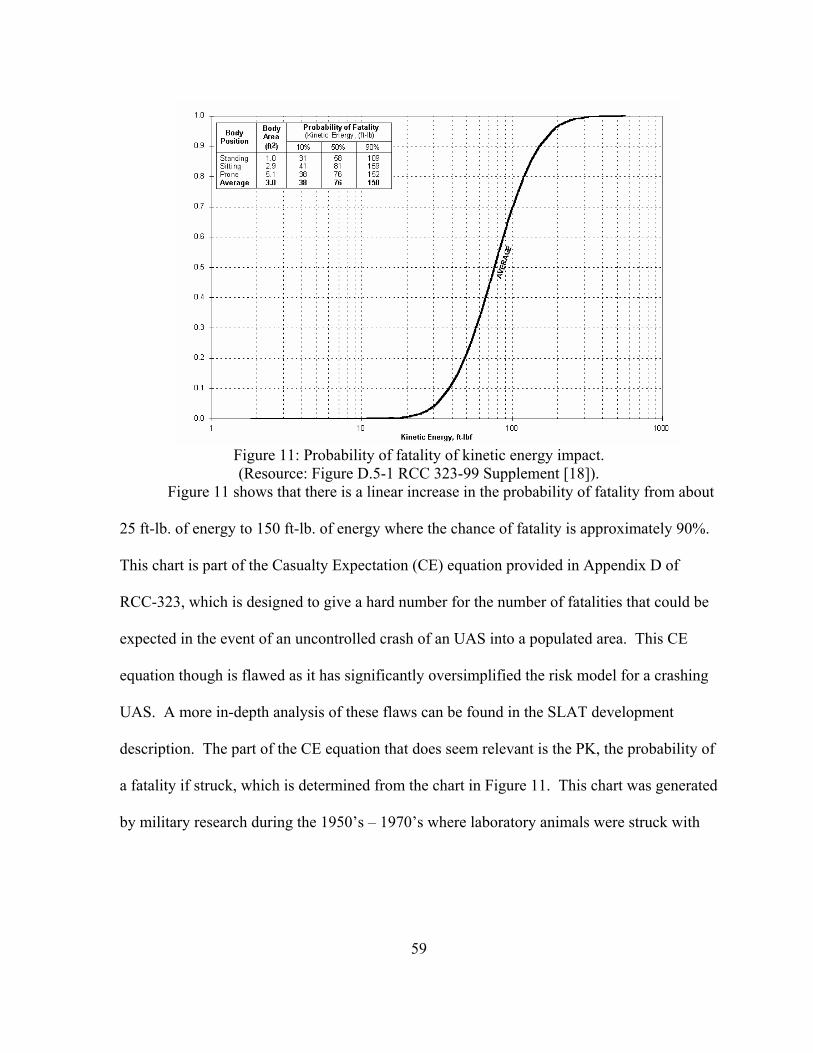
59

Figure 11: Probability of fatality of kinetic energy impact. (Resource: Figure D.5-1 RCC 323-99 Supplement [18]).

Figure 11 shows that there is a linear increase in the probability of fatality from about

25 ft-lb. of energy to 150 ft-lb. of energy where the chance of fatality is approximately 90%.

This chart is part of the Casualty Expectation (CE) equation provided in Appendix D of

RCC-323, which is designed to give a hard number for the number of fatalities that could be

expected in the event of an uncontrolled crash of an UAS into a populated area. This CE

equation though is flawed as it has significantly oversimplified the risk model for a crashing

UAS. A more in-depth analysis of these flaws can be found in the SLAT development

description. The part of the CE equation that does seem relevant is the PK, the probability of

a fatality if struck, which is determined from the chart in Figure 11. This chart was generated

by military research during the 1950’s – 1970’s where laboratory animals were struck with

60

various objects at various speeds. The trends seen in those studies were extrapolated to

generate Figure 11.

Samples of Lethality Using Approach #1

To see how this lethality approach relates to actual UAS being used currently by the

armed forces the equation was rearranged to show velocity versus weight. Figure 3 below

shows 10% and 90% lethality boundaries for a number of small UAS. All UAS are plotted at

their maximum listed operating speed. The worst case impact speed would push the points to

the right by 40%

Figure 12: Sample UAS with 10% Lethal Boundary (blue dashed line) and 90% Lethal Boundary (pink dashed line). UAS data compiled from [24].

61

Figure 12 shows fairly clearly that all the current UAS above 2 pounds are more than

90% lethal using this approach. The two smaller vehicles below the 10% lethal boundary are

both typically qualified as MAVs and appear to be the only UAS that can claim some level of

reduced lethality. Given that UAS will likely impact with velocities higher than their max

operating speeds (further to the right on figure 12) it is suggested that any UAS above the 2

pound mark should be considered capable of causing life threatening injuries.

Kinetic Energy Approach #2

The second approach models energy density and the relative masses of the vehicle

and target. This method is most often used in analysis of less-than-lethal weapons such as

riot suppression bean-bag loads and rubber bullets for shotguns. This approach has also been

applied to evaluating injuries due to KE transfer through soft body armor and the U.S. Army

has produced several reports that attempt to make a KE to lethality correlation.

A 1976 report “Blunt Trauma Data Correlation” used live domesticated animals as

test subjects [26]. The animals were shot in the thorax with various objects (noncompliant

cylinders, stun bags, stun rags, etc.) weighing between 50 and 200 grams at a variety of

velocities. The animals were left untreated for 24 hours to see if they died from the injuries.

The result of this study was a correlation that involved the diameter of the cylinder as a key

factor. This variable relates to energy density since with small projectiles the interaction area

is so small that all of the energy transfer is localized and much more likely to cause serious

injury.

62

Overall, the energy density approach seems to work very well for small high speed

projectiles such as stun bag loads, but it does not appear to be a particularly good approach

for modeling UAS injuries. The largest projectiles examined were significantly smaller than

the UAS being examined and were fired at significantly higher velocities. The results from

[26] were already extrapolated from the animal subject average weight of about 30 kg to the

70 kg average weight of an adult. Further extrapolating the trend to larger and slower

projectiles would severely decrease the confidence in that trend.

This research can be collaborated by an Army Research Lab study performed in 1999

(ARL-TR-1868) [27] that correlated lethality based on KE transfer into clay blocks. This

study was examining non-lethal weapons technology so it also used low mass projectiles and

built upon the 1975 reports lethality model. That study produced a very useful chart shown

below as figure 13.

Figure 13: Lethality ranges for various projectile and target parameters from [27].

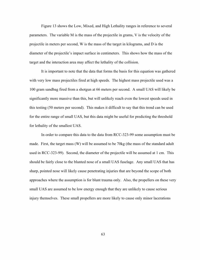
63

Figure 13 shows the Low, Mixed, and High Lethality ranges in reference to several

parameters. The variable M is the mass of the projectile in grams, V is the velocity of the

projectile in meters per second, W is the mass of the target in kilograms, and D is the

diameter of the projectile’s impact surface in centimeters. This shows how the mass of the

target and the interaction area may affect the lethality of the collision.

It is important to note that the data that forms the basis for this equation was gathered

with very low mass projectiles fired at high speeds. The highest mass projectile used was a

100 gram sandbag fired from a shotgun at 66 meters per second. A small UAS will likely be

significantly more massive than this, but will unlikely reach even the lowest speeds used in

this testing (50 meters per second). This makes it difficult to say that this trend can be used

for the entire range of small UAS, but this data might be useful for predicting the threshold

for lethality of the smallest UAS.

In order to compare this data to the data from RCC-323-99 some assumption must be

made. First, the target mass (W) will be assumed to be 70kg (the mass of the standard adult

used in RCC-323-99). Second, the diameter of the projectile will be assumed at 1 cm. This

should be fairly close to the blunted nose of a small UAS fuselage. Any small UAS that has

sharp, pointed nose will likely cause penetrating injuries that are beyond the scope of both

approaches where the assumption is for blunt trauma only. Also, the propellers on these very

small UAS are assumed to be low energy enough that they are unlikely to cause serious

injury themselves. These small propellers are more likely to cause only minor lacerations

64

before breaking off. Using these assumptions the following calculation for Low Lethality

can be made:

70 1 4.2

13: 4.2 11.8

.

12

.

2000

66.6 49.1

With the simplifications and rounding to the nearest foot-pound the data from [27]

shows that a safe nonlethal kinetic energy threshold with only a low chance of lethality

would be below 49 ft-lb.

This research suggests that the nonlethal range for MAVs be considered below 2

pounds of weight, less than 49 foot-pounds of kinetic energy (based on maximum take-off

weight and maximum operating speed), and have a maximum operating speed of 100 feet per

second. It is further expected that the KE increase during a crash for vehicles below 2 lb will

be proportionally lower than for larger UAS thus using the maximum operating speed should

therefore be a good estimate of the maximum KE for the MAV. The maximum operating

speed of 100 feet per second was chosen to avoid any aircraft that might better be described

as guided projectiles or kinetic micro-munitions. Any MAV with an operating speed over

100 feet per second (nearly 70 mph) would need to be examined independently as its ability

to cause penetrating injuries would be significantly high. Plotting this nonlethal range

65

produces the shaded box shown in figure 14 below. Several UAS near this boundary have

been plotted to show how this nonlethal UAS range correlates to current systems.

Figure 14: Nonlethal Range (grey shaded area) with sample MAVs and Small UAS

From Figure 14 it is clear that a large number of the vehicles known as all fall into

this nonlethal range. There are some larger MAVs that are outside of this range (blue circle).

It should be noted that these lethality studies all assume non-compliant projectiles. Most of

these airframes are actually made of EPC foam, which would be partially compliant in an

impact scenario. Aircraft above the 49 ft-lb threshold, but less than 2 lb MTOW should be

Common Hand Launched UAS

Foam Bodied MAVs

66

examined on a case-by-case basis to determine how much threat they actually pose to people

on the ground. The 49 ft-lb threshold is designed to be quite conservative and corresponds to

a PK value of approximately 0.2 or 20% chance of lethality from the lethality estimation in

RCC-323-99 as shown in figure 15 below.

Figure 15. Red Line Indicates 49 ft-lb Threshold in Relation to RCC-323-99 Lethality Estimate

Conclusion for Crash Lethality

The separation between nonlethal and lethal energy thresholds is small enough that

the lethality of small UAS can be modeled as a binary grouping instead of a continuous

function. Any vehicle under 49 foot-pounds of energy and two pounds can be considered

67

nonlethal, while anything outside of that range should be considered capable of causing life

threatening injuries during an uncontrolled crash. Based on this result SLAT will be limited

to above the nonlethal range so it will only be applicable to UAS between 2 and 350 lb.

68

CHAPTER 4

Algorithm Development

The Target Level of Safety (TLS) is the threshold that all of the various UAS

domains are trying to earn points to reach. This threshold is derived using the CE equation

from [18] as a starting point. The original CE equation from [18] is modified to avoid having

to determine directly a system level failure rate at a high level of confidence. The final TLS

equations maps into point space that varies from 1 to 10,000 points across the small UAS

category based on the size of the aircraft and the population density of the mission area.

The top-end value of 10,000 points was chosen to make the point values in SLAT

easy to understand while still giving good resolution between different types of tests. SLAT

is designed such that most of the tests in SLAT range from 20 to 500 points. This avoids the

proponents having to deal with fractions of points or with tens of thousands of points. The

TLS algorithm is tuned such that the value of 10,000 points represents the TLS required for a

350 lb, 15 ft wingspan UAS to fly 100% of its mission over an open air assembly of people.

This was viewed as a theoretical “worst-case” type aircraft and mission. This theoretical

aircraft was designed to be slightly larger than current operational 330 lb. UAS, which has

approximately a 13 foot wingspan and weighs roughly 330 lb. MTOW. Since the TLS

scales with both weight and wingspan this top-end aircraft is important for tuning, but it

doesn’t set a hard limit based on wingspan alone. SLAT would still be applicable to aircraft

with larger wingspans if the weight was lower. It is expected that any aircraft over 150 kg

69

will be following STANAG 4671 rather than SLAT so having a UAS above the tuning range

is unlikely.

If aircraft significantly larger than the top-end aircraft were applied to SLAT it is

possible that the tool would begin to lose its effectiveness. Their size and weight would

likely cause the TLS values to be above 10,000 points for flights over OAA. The point

allocation algorithm (section 4.3) is designed to map back to 10,000 points for addressing all

of the Catastrophic and Critical failure modes. This algorithm guarantees that there are

enough points available to reach any TLS below 10,001 points. Although it is possible to get

more than 10,000 points aircraft significantly outside of the design range may find it

impossible to earn enough points to reach their TLS. It is due to this constraint that the

designer recommends not applying SLAT to aircraft over 15 ft wingspan and 350 lb. without

first modifying the point allocation algorithm to reflect the new top-end condition.

4.1 TLS Algorithm Derivation

The TLS algorithm is derived from the Casualty Expectation (CE) equation in the

Appendix D of [18]. The CE equation was derived from first principles based on

multiplication of point estimates for the different risk variables. Equation 1 below shows the

equation as it is found in [18].

(1)

Where: PF = Probability of Failure (failures per flight hour) PD = Population Density of Mission Area (people per square mile) AL = Lethal Area (square feet) PK = Probability of Killing Someone if hit (dimensionless)

70

S = Shelter Factor (dimensionless) Unfortunately, as discussed previously, it is easy to make a units mistake in the original

equation due to multiplying the PD variable (in units of people per square mile) by the AL

variable (in units of square feet). This error can be easily corrected by dividing the

population density variable by the number of square feet in a square mile (roughly 27.8

million) as shown in Equation 2 below. The PD variable has been replaced with ρ to denote

the time weighted average of the mission area using the population density categories

discussed in Section 3.5. Also the AL variable has been replaced with the impact model

discussed in section 3.6. Furthermore, since SLAT is limiting its scope to aircraft about 2 lb.

MTOW the PK (probability of fatality if struck) variable can be set to one as discussed in

section 3.7.

.

1 (2)

The PF variable represents the system level probability of a failure that leads to the crash

of the UAS. This can be a very difficult variable to define with any certainty for this

category of aircraft. Due to the limited history and use of hobby grade components, very few

UAS can estimate their top level failure rate with any degree of accuracy. The reliability

data for many of the components simply doesn’t exist and performing such in-depth

reliability studies would push the cost of small UAS to that of manned aircraft making them

economically infeasible.

The Shelter Factor variable (S) can be viewed as two distinct components: hard shelter

and soft shelter. Hard shelter refers to those buildings and cover that will provide protection

from even the heaviest of the aircraft in the small UAS category (e.g. multistory concrete

71

wall buildings), while soft shelter includes the protection provided by items such as trees or

being in a car. Soft shelter may provide some shelter from the smallest UAS in the small

UAS category, but may not provide much shelter at all as the aircraft size approaches 350 lb.

If a 3 lb. UAS were to crash into a car it responsible to expect that it wouldn’t injury the

people inside, but if a 300 lb. UAS were to crash into the same car it is not unreasonable to

expect that anyone inside would have received life-threatening injuries. Quantifying this

shelter factor though proves to be very difficult. In the original CE equation it can be varied

between 0 (everyone is sheltered) to 1 (no one is sheltered), and the choice of this variable

can have a huge effect on the overall result. In the development of SLAT it was decided to

handle the shelter component differently. The hard shelter component is contained in the

assumptions made during the creation of the population density categories. The primary

assumption is that all yellow “observable urban” areas can be treated as having the same

exposed population density of 9,800 per square mile. The assumption is made on the

principle that as population density increases the amount of hard shelter increases

proportionally (i.e. the only way to get really high population densities is to put people

vertically in buildings that will provide protection from any aircraft in the small UAS

category). The soft shelter component will be brought back into the TLS equation at a later

step, but for now it will be set aside.

The acceptable casualty rate (the CE variable) can really be seen as the ELS or equivalent

level of safety mentioned earlier. This is the base risk that all people have of being killed by

a crashing conventional aircraft. Thankfully that probability is very low, 1x10-7 per flight

72

hour. For UAS operations in the NAS to be acceptable it will have to be shown that they

pose no greater risk to the people on the ground than that posed by conventional aircraft.

Therefore, the CE variable in Equation 2 can be replaced by the ELS value of 1x10-7 as

shown in equation 3 below.

10.

(3)

This can be rearranged to bring PF to the right hand side of the equation as shown in

Equation 4.

.

. (4)

The inverse of Equation 4 (Equation 5 below) gives the Mean Time Between Failures

(MTBF) that meets the ELS of one fatality every ten million flight hours based on the

population density of the mission area and the size of the aircraft. This shows that MTBF is

proportional to the risk variables ρπb2.

.

(5)

The next step is to take the log of those risk variables and square the result (see

Equation 6 below). This squaring step was added to mimic the requirements for manned

aircraft where the requirements are more heavily biased against the larger aircraft. The effect

in SLAT is that as the aircraft approach higher and higher wingspans they are required to

meet higher and higher levels of airworthiness.

73

(6)

The TLS equation is almost finished at this point except for the soft shelter

component. Soft shelter can be viewed as a function of the KE of the crashing aircraft. Soft

shelter will be proportionally less effective as the KE in the crashing UAS increases. There

will clearly be some transfer of PE to KE during an aircrafts uncontrolled descent, but it is

difficult to quantify exactly what that amount would be. SLAT makes a further assumption

that all the UAS in the small UAS category are going to reach effectively the same terminal

velocity during an uncontrolled crash. With this assumption the KE variation between the

different aircraft is reduced to a function of it mass or weight. The soft shelter component is

then taken into account by adding the variable W (aircraft weight) to the TLS algorithm as

shown in Equation 7 below. Without the weight scaling a 20 lb. glider-type UAS with a 10

foot wingspan would require the same TLS as a 300 lb. UAS that also had a 10 foot

wingspan. Clearly the 300 lb. aircraft poses more of a threat than the 20 lb. aircraft.

(7)

The final step in the TLS algorithm derivation is to adjust the top level situation of a

15 ft wingspan, 350 lb. aircraft flying 100% of its mission over open air assembly to map to

10,000 points. This is done through a tuning variable k that is set to 0.4643.

0.4643 (8)

Equation 8 is the final form of the TLS algorithm. The final value is always rounded

to the nearest whole number since SLAT doesn’t use fractions of points. As an example

assume that an 8 ft wingspan aircraft that has a MTOW of 55 lb. is flying the example traffic

74

monitoring mission described in section 3.5. The population density (ρ) from the example

mission is 8,870 people per square mile as shown in Table 3. Equation 9 below shows the

TLS derivation for this example aircraft flying the traffic monitoring mission.

0.4643 55 8870 8 998 (9)

This shows that this 8 ft wingspan, 55 lb. aircraft would need to earn at least 947 points in

every domain to be considered airworthy. To contrast let’s examine a UAS half the size of

the first example flying the same mission. Equation 10 shows the TLS for this smaller UAS.

0.4643 27.5 8870 4 407 (10)

This shows how a smaller UAS would be required to show fewer artifacts to be considered

safe to fly the same mission.

Since the TLS is dependent on aircraft parameters (weight and wingspan) it is not

feasible to calculate the TLS for a given mission without knowing the aircraft performing it.

Section 6.3 has examples of applying this algorithm to three of the missions discussed in

Section 3.3 (Stadium Fly-over, Butner: First Flight, Butner: Picnic).

4.2 Operational Flight Hours

Since there are many small UAS currently in service there is naturally a question of

how those flight histories are accounted for in SLAT. The UAS industry tends to rely

heavily on how many successful flight hours a system flow, but it is very difficult to account

for operational hours directly (i.e. 3 pts per successful flight hour) since the data is very

incoherent. There is typically very little information saying what the environmental

75

conditions were during the flights, how the missions were performed, or the configuration of

the UAS. Obviously flight tests give very good information about how the system functions,

but incoherent data brings with it a large amount of uncertainty. A flight test that takes the

aircraft to the extent of its operational range is very useful for verifying the different

domains. Suppose, for example, that a flight goes to 95% of the range of the ground station

command/control link. Showing that the link was stable up to this extent gives good

validation that the design range has been met. It could be argued that operational flight hours

also validate the command/control link, but 50 hours at 95% of the design range is

significantly different than 50 hours flying within line of sight of the ground station. This

illustrates the danger of relying on operational flight hours to prove a system. Simply

knowing that the aircraft has flown for some length of time doesn’t tell a CA how much of

the flight envelope was covered. All of the operational hours could have been flown on clear

days with no wind and well within the range of the ground station. On the other hand, the

operational hours could have been performed in weather outside of the design specification

and truly pushed the limits of the system. The problem is that without coherent data a CA

must make conservative assumptions about what operational flight hours tell them about the

overall system reliability.

One way to be conservative on this type of estimation is to use a χ2 (Chi-squared)

approach to determine the lower 95% confidence bound based on hours flown and the

number of mishaps. A lower 95% confidence states that there is only a 5% chance that the

actual system failure rate is worse than this lower bound. Appendix E contains three detailed

76

approaches to calculating the percent confidence bounds depending on the amount of

information available. One approach handles how to calculate the lower 95% confidence

bound given X number of flight tests hours without any failures. The other two approaches

focus on flight test data with observed failures.

Obviously having no failures during operational flights is very unlikely, but it would

seem to say that the system is very safe. Unfortunately, the number of hours needed to show

an acceptable failure rate is excessive even for rather lenient failure rates. For example, let’s

assume that a small UAS is trying to show an acceptable failure rate through operational

flight hours to fly in an unpopulated area. To have a 95% confidence that the system had

indeed met the required failure rate of 1.93x10-3 failures per flight hour the system would

have to show 1550 hours of operational flight hours with no failures. To reach the 95%

confidence for a failure rate of 1x10-6 failures per flight hour a system would require 2.9

million hours of operation without any failures. Obviously, if the number of hours needed

to certify the reliability of the aircraft is an order of magnitude greater than the expected

entire operational fleet life of the aircraft then trying to certify through operational flight test

hours is not a feasible approach.

The inconsistency and incoherent data of operational flight hours forces the use of

conservative assessment of those hours’ contributions to the overall system safety. SLAT

grants no points for operational flight hours because the number of hours needed to provide a

significant contribution to the system safety is so high as to be unrealistic and there is no way

to determine how points should be allocated across the different domains. SLAT does grant

77

large amounts of points for engineering flight tests where coherent data is collected to show

precisely how much of the operational envelope has been verified. As shown in section 3.3

SLAT views flight testing as the best validation method, granting in general three times as

many points for flight test verification for a failure mode compared to a purely analytical

method.

4.3 Point Allocation Algorithm

The next key component of SLAT is how the points are determined for each of the

tests performed. The maximum points available for any one test is based on the criticality of

the failure modes addressed by that test derived directly from the tailored FMECA for a

specific UAS. It is generally understood that testing of actual components greatly increases

the confidence in the final product over purely analytical approaches or simulations. The

most useful information in airworthiness comes from engineering flight tests of the actual

aircraft system. It is very difficult to quantify exactly how that confidence increases, but

SLAT attempts to capture it by granting twice as many points for physical testing of

components and three times as many points for flight testing of components as compared to

pure analysis.

SLAT is designed to be very flexible for both varying standards and verification

methods. An example of a standard for structures would be building structures to a 1.25

factor of safety versus the manned aviation standard of 1.5. For verification methods an

example would be picking up an aircraft by the wing tips to test the wing’s strength versus a

78

static load test to failure of a flight article to determine the load at which the wings actually

fail. Tests that meet the manned aviation standard or verification methods warrant the

highest number of points, while tests that fall short of the manned requirements are penalized

by receiving fewer possible points. The penalty for reducing the verification method is twice

the penalty for reducing the standard. This is an attempt to capture the reduction in

confidence as verification methods are reduced. It is preferable to know with a high degree

of confidence that some component has actually meet some lesser standard than to have a

low confidence that it has meet some higher standard. For example, an aircraft could be

designed with the manned standard of a 1.5 factor of safety for all of the structures, but if the

verification method is only an email from the designer stating that it was designed to that

level then the CA will likely have very little confidence that the aircraft actually has meet

that standard.

For each test the developer must first determine the confidence slot that it is fulfilling

(Analysis, Physical, or Flight Test). Next, the developer determines which failure modes are

being addressed along with the standard and verification methods being used. The final step

is to sum the points for granted for each failure mode to determine the final point value of the

test. This algorithm is shown in figure 16.

79

 

Figure 16: Point Allocation Algorithm The value of 6 in the denominator is there to normalize across the three confidence

categories. The goal for tuning was that 10,000 points accounts for addressing all Critical

and Catastrophic failure modes in all three confidence slots. Ncrit is the number of Critical

failure modes and Ncat is the number of Catastrophic failure modes. The confidence slots

have scaling of 1, 2, and 3 for Analysis, Physical Tests, and Flight Testing respectfully. The

6 in the denominator is the sum of those scaling factors.

Appendix B of this document contains over 20 example tests based on the tailored FMECA

sets for each of the 5 example aircraft discussed in Chapter 5. Section 6.2 contains several

detailed examples of how to use the Point Allocation Algorithm to derive SLAT tests.

4.3.1 Grading Tests

There are several difficulties that cannot be addressed by this point allocation

algorithm. One situation occurs when an artifact shows that a test was poorly conducted.

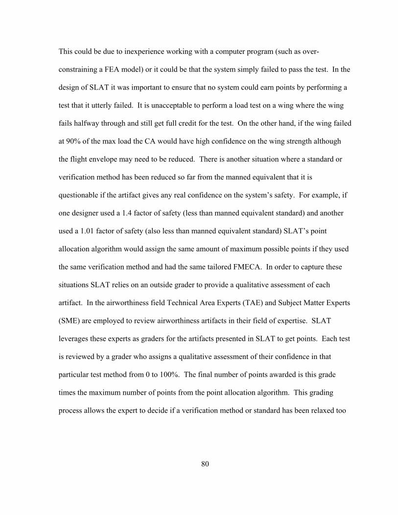
80

This could be due to inexperience working with a computer program (such as over-

constraining a FEA model) or it could be that the system simply failed to pass the test. In the

design of SLAT it was important to ensure that no system could earn points by performing a

test that it utterly failed. It is unacceptable to perform a load test on a wing where the wing

fails halfway through and still get full credit for the test. On the other hand, if the wing failed

at 90% of the max load the CA would have high confidence on the wing strength although

the flight envelope may need to be reduced. There is another situation where a standard or

verification method has been reduced so far from the manned equivalent that it is

questionable if the artifact gives any real confidence on the system’s safety. For example, if

one designer used a 1.4 factor of safety (less than manned equivalent standard) and another

used a 1.01 factor of safety (also less than manned equivalent standard) SLAT’s point

allocation algorithm would assign the same amount of maximum possible points if they used

the same verification method and had the same tailored FMECA. In order to capture these

situations SLAT relies on an outside grader to provide a qualitative assessment of each

artifact. In the airworthiness field Technical Area Experts (TAE) and Subject Matter Experts

(SME) are employed to review airworthiness artifacts in their field of expertise. SLAT

leverages these experts as graders for the artifacts presented in SLAT to get points. Each test

is reviewed by a grader who assigns a qualitative assessment of their confidence in that

particular test method from 0 to 100%. The final number of points awarded is this grade

times the maximum number of points from the point allocation algorithm. This grading

process allows the expert to decide if a verification method or standard has been relaxed too

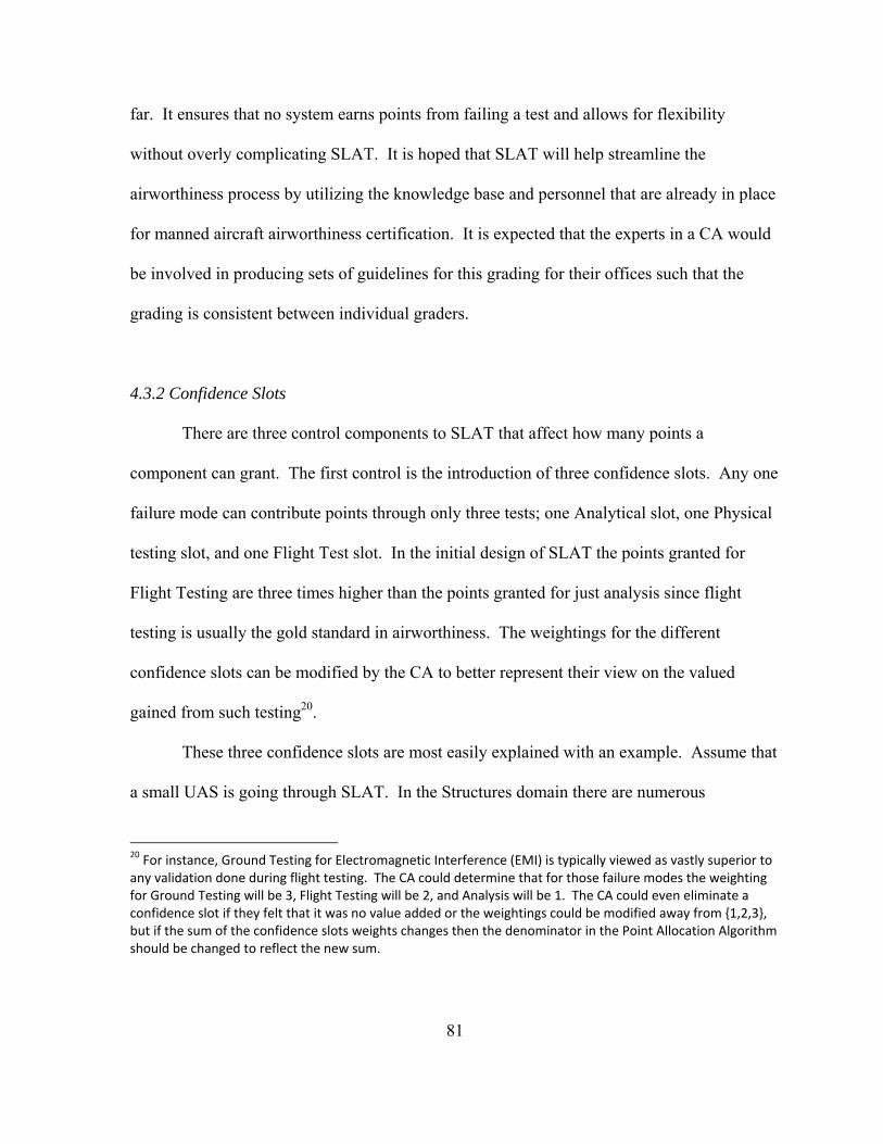
81

far. It ensures that no system earns points from failing a test and allows for flexibility

without overly complicating SLAT. It is hoped that SLAT will help streamline the

airworthiness process by utilizing the knowledge base and personnel that are already in place

for manned aircraft airworthiness certification. It is expected that the experts in a CA would

be involved in producing sets of guidelines for this grading for their offices such that the

grading is consistent between individual graders.

4.3.2 Confidence Slots

There are three control components to SLAT that affect how many points a

component can grant. The first control is the introduction of three confidence slots. Any one

failure mode can contribute points through only three tests; one Analytical slot, one Physical

testing slot, and one Flight Test slot. In the initial design of SLAT the points granted for

Flight Testing are three times higher than the points granted for just analysis since flight

testing is usually the gold standard in airworthiness. The weightings for the different

confidence slots can be modified by the CA to better represent their view on the valued

gained from such testing20.

These three confidence slots are most easily explained with an example. Assume that

a small UAS is going through SLAT. In the Structures domain there are numerous

20 For instance, Ground Testing for Electromagnetic Interference (EMI) is typically viewed as vastly superior to any validation done during flight testing.  The CA could determine that for those failure modes the weighting for Ground Testing will be 3, Flight Testing will be 2, and Analysis will be 1.  The CA could even eliminate a confidence slot if they felt that it was no value added or the weightings could be modified away from {1,2,3}, but if the sum of the confidence slots weights changes then the denominator in the Point Allocation Algorithm should be changed to reflect the new sum. 

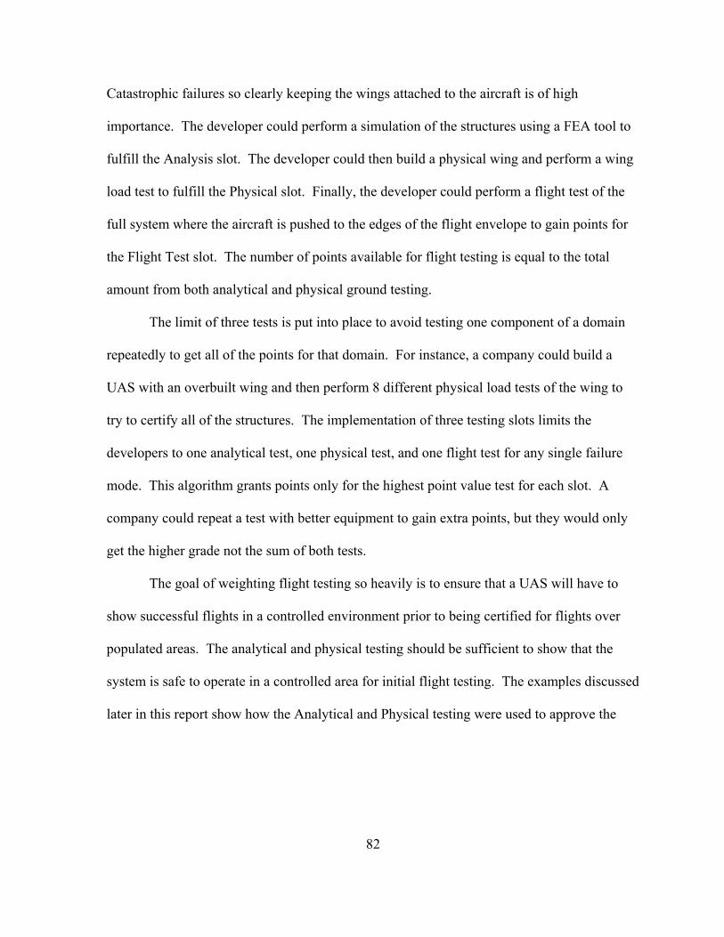
82

Catastrophic failures so clearly keeping the wings attached to the aircraft is of high

importance. The developer could perform a simulation of the structures using a FEA tool to

fulfill the Analysis slot. The developer could then build a physical wing and perform a wing

load test to fulfill the Physical slot. Finally, the developer could perform a flight test of the

full system where the aircraft is pushed to the edges of the flight envelope to gain points for

the Flight Test slot. The number of points available for flight testing is equal to the total

amount from both analytical and physical ground testing.

The limit of three tests is put into place to avoid testing one component of a domain

repeatedly to get all of the points for that domain. For instance, a company could build a

UAS with an overbuilt wing and then perform 8 different physical load tests of the wing to

try to certify all of the structures. The implementation of three testing slots limits the

developers to one analytical test, one physical test, and one flight test for any single failure

mode. This algorithm grants points only for the highest point value test for each slot. A

company could repeat a test with better equipment to gain extra points, but they would only

get the higher grade not the sum of both tests.

The goal of weighting flight testing so heavily is to ensure that a UAS will have to

show successful flights in a controlled environment prior to being certified for flights over

populated areas. The analytical and physical testing should be sufficient to show that the

system is safe to operate in a controlled area for initial flight testing. The examples discussed

later in this report show how the Analytical and Physical testing were used to approve the

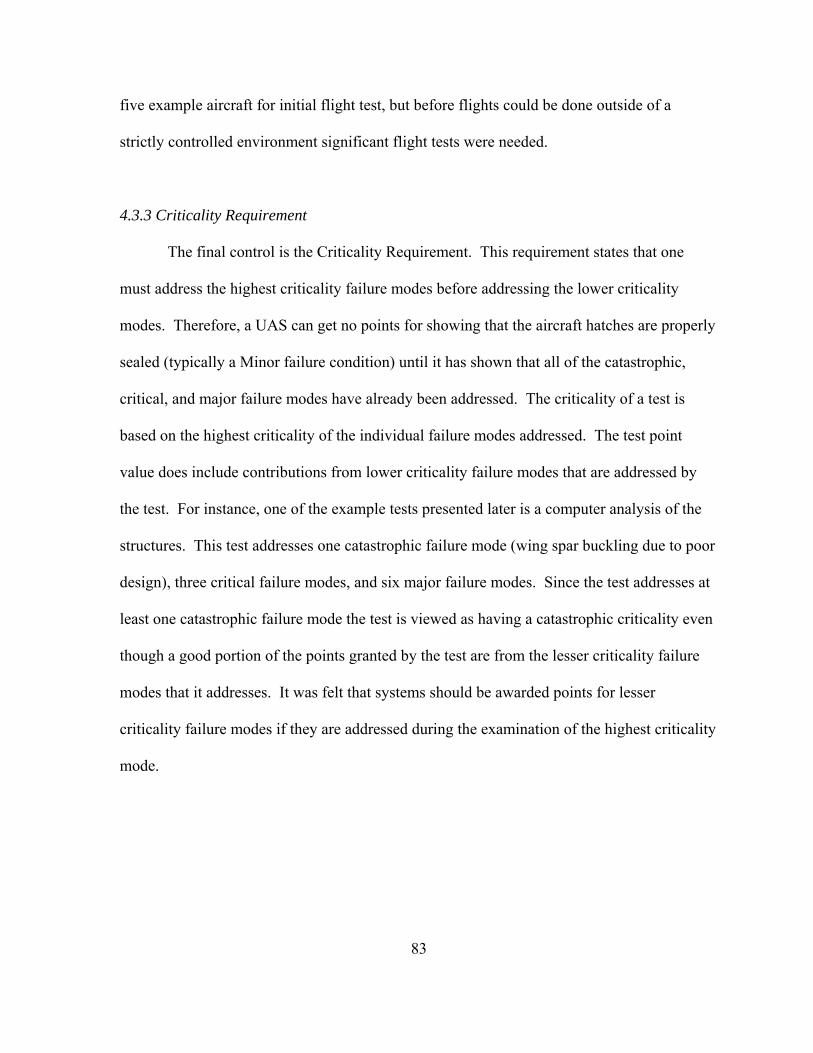
83

five example aircraft for initial flight test, but before flights could be done outside of a

strictly controlled environment significant flight tests were needed.

4.3.3 Criticality Requirement

The final control is the Criticality Requirement. This requirement states that one

must address the highest criticality failure modes before addressing the lower criticality

modes. Therefore, a UAS can get no points for showing that the aircraft hatches are properly

sealed (typically a Minor failure condition) until it has shown that all of the catastrophic,

critical, and major failure modes have already been addressed. The criticality of a test is

based on the highest criticality of the individual failure modes addressed. The test point

value does include contributions from lower criticality failure modes that are addressed by

the test. For instance, one of the example tests presented later is a computer analysis of the

structures. This test addresses one catastrophic failure mode (wing spar buckling due to poor

design), three critical failure modes, and six major failure modes. Since the test addresses at

least one catastrophic failure mode the test is viewed as having a catastrophic criticality even

though a good portion of the points granted by the test are from the lesser criticality failure

modes that it addresses. It was felt that systems should be awarded points for lesser

criticality failure modes if they are addressed during the examination of the highest criticality

mode.

84

CHAPTER 5

Example Aircraft

To illustrate how SLAT would be used 5 example aircraft are shown over the next

few sections through the process of FMECA tailoring (Section 6.1), TLS calculation (Section

6.2), and Point Allocation for Tests (Section 6.3).

5.1 NC State Aerospace Engineering Senior Design Program

All five of the aircraft being used as examples are products of the Aerospace

Engineering Senior Design course. This capstone course is comprised of two semesters. At

the beginning of the fall semester the students are broken into teams of 7 and 10 individuals

and given a list of customer requirements for an UA. They spend the fall semester

performing the design and analysis of an aircraft to meet those requirements and they must

successfully complete a Critical Design Review (CDR) at the end of the fall semester in

order to move on to the spring semester. During the spring semester the students are

responsible for building and testing the aircraft that they designed the previous semester.

The aircraft go through a First Flight Readiness Review (FFRR) to demonstrate that they are

ready for flight. A significant part of the FFRR process is comparison of ground test results

with the design predictions. The customer requirements typically limit the size to below 30

lb. such that the vehicles can be tested at Perkins Field. This course has a “fly or fail”

85

requirement such that if the aircraft doesn’t fly, then the whole team would fail the senior

design course.

This capstone course has been in place for 31 years and has produced many aircraft

with good flight characteristics. SLAT leverages NCSU Flight Research’s experience

gathered from these years of aircraft design, manufacture, and flight testing. The seniors are

required to submit many different artifacts from their design, analysis, and testing. The

application of SLAT uses these course deliverables as the artifacts for earning points. The

example aircraft chosen were from recent years where digital copies of their CDR documents

were available for distribution with this report. It is hoped that providing theses example

artifacts will help clarify how SLAT could be applied to other systems. All five of the

example aircraft described in the next sections were built by the students and flown

successfully as part of the spring semester of the senior design course.

The aircraft designed and built during the senior design course are controlled by a

remote pilot like a standard hobby radio controlled (RC) airplane. Although many of the

aircraft are designed to accommodate the Piccolo autopilot budget and time constraints make

adding an autopilot to each aircraft unreasonable. As a demonstration of SLAT a second

configuration will be examined with the addition of an autopilot to make the aircraft

autonomous. To avoid delving into proprietary aspects of a specific autopilot this report

examines adding a generic autopilot of complexity and functionality roughly equivalent to a

Piccolo autopilot. Some key assumptions have to be made about the complexities and

86

abilities of this generic autopilot. To make things simple the following assumptions were

made about the generic autopilot:

• It contains a magnetometer (nFC component)

• It contains 3 single axis accelerometers (all 3 separate FC components)

• It contains 3 single axis gyros (all 3 separate FC components)

• It contains a single GPS antenna and module (FC component)

• The internal software onboard aircraft has 10 FC sections of code

• The control laws (part of Control System – Math FMECA) are viewed as a single FC

component.

• The ground station is assumed to be a single laptop and falls into the category of

“Portable”

The five example aircraft share some common equipment in the “Remote Control” (RC)

configuration. All aircraft are using standard hobby transmitters, receivers, and servos as

well as an EagleTree data recorder and a camera payload (both the data recorder and camera

are considered to be non-Flight Critical (nFC)21.

21 Flight Critical (FC) components are those that a failure is likely to result in the loss of the aircraft while the failure of non‐Flight Critical (nFC) components is expected to result in reduced performance.  For example, the rudder is considered to be a nFC control surface, while the elevator is considered a FC control surface.  Likewise, lights to help avoid mid‐air collisions are considered nFC even though the loss of the external lighting may greatly increase the overall risk of the system (the loss of the lights wouldn’t directly result in the loss of the aircraft). 

87

5.2 Three “Backpack-able” UAS

The customer requirements for the senior design class of 2008-2009 were focused on

creating small “backpack-able” reconnaissance aircraft. Each aircraft had to disassembled

and stored in a 1.5 ft2 box, assembled and be ready for flight by a two person team in five

minutes, launch from and recover in unimproved fields, be able to land on paved surfaces, be

able to carry a video camera payload, and be capable of carrying and integrating a Piccolo

autopilot. A further requirement that the aircraft and the storage box could be no more than

10 lb. limited the aircraft sizes. There were three teams during this year that created three

unique aircraft: Phoenix, Optikos, and Piolin.

88

5.2.1 Phoenix

Phoenix, shown in figure 12 below, has a straight wing with dual booms going back

to an inverted V-tail. It has two servos in the wing and two servos in the tail. It was

launched from a bungee cord powered rail launcher that collapsed down into its own 1.5 ft2

box. Phoenix has four FC control surfaces and zero nFC control surfaces.

   

Figure 17: Phoenix (Team 1, 2008-2009). CAD drawing (Left) and During Launch (Right)

Table 7: Phoenix Dimensions (Team 1, 2008-2009)

Wingspan: 5.7 ft

Weight: 6.04 lb.

Flight Critical Control Surfaces: 2

Non-Flight Critical Control Surfaces: 2

89

5.2.2 Optikos

Optikos is a flying wing (see figure 10) with only two control surfaces. The winglets

are flat plates that bolt on the end of the wing and have no control surfaces. It used the same

launcher system as Phoenix and had skids for belly landings on the runway. Optikos has

only two control surfaces, both of which are FC.

Figure 18: Optikos (Team 3, 2008-2009). Shown here on the launcher used by both Optikos and Phoenix (Right) and held by a team member (Left).

Table 8: Optikos Dimensions (Team 3, 2008-2009) Wingspan: 5.43 ft

Weight: 6.3 lb.

Flight Critical Control Surfaces: 2

Non-Flight Critical Control Surfaces: 0

90

5.2.3 Piolin

Piolin was a conventional design (see figure 11) that was hand launched and had

skids for a belly recovery. Piolin has three FC control surfaces and one nFC control surface.

   

Figure 19: Piolin (Team 2, 2008-2009). CAD rendering of aircraft (left) and during hand launch (right).

Table 9: Piolin Dimensions (Team 2, 2008-2009) Wingspan: 6 ft

Weight: 4.6 lb.

Flight Critical Control Surfaces: 3

Non-Flight Critical Control Surfaces: 1

5.3 Jet Powered Example UAS

For eight years the senior design course focused on building jet powered aircraft

using AMT Mercury micro-turbojets. In 2005-2006 the customer requirements were to build

a jet with thrust vectoring and the aircraft Hyperion was one of the aircraft from that year. In

2007-2008 the customer requirements focused on high reliability. The aircraft Goose is one

of the aircraft from the 2007-2008 year. The two jets are here as examples to show how the

91

increase in complexity and weight propagates through SLAT and results in more stringent

requirements.

5.3.1 Hyperion

Hyperion, shown below in Figure 12, has a mostly conventional design with an H-

tail, tricycle landing gear equipped with pneumatic brakes, and thrust vectoring in both pitch

and yaw. The thrust vectoring nozzle is considered an addition set of two nFC control

surfaces resulting in Hyperion having 8 nFC control surfaces and 2 FC control surfaces.

   

Figure 20: Hyperion (Team 1, 2005-2006).  

Table 10: Hyperion Dimensions (Team 1, 2005-2006) Wingspan: 5.19 ft

Weight: 27 lb.

Flight Critical Control Surfaces: 2

Non-Flight Critical Control Surfaces: 8

92

5.3.2 Goose

Goose appears to be very similar to Hyperion (sans the thrust vectoring system), but

the critical difference is that Goose is designed to be able to fly with the loss of any one

control surface. This design feature is reflected in the FMECA tailoring, which is the first

step in SLAT. Goose has zero FC control surfaces and 8 nFC control surfaces.

 

 

Figure 21: Goose (Team 3, 2007‐2008).  

Table 11: Goose Dimensions (Team 3, 2007-2008) Wingspan: 6.5 ft

Weight: 34 lb.

Flight Critical Control Surfaces: 0

Non-Flight Critical Control Surfaces: 8

93

CHAPTER 6

Application of SLAT to Example Aircraft

6.1 FMECA Tailoring

The first step in using SLAT is to tailor a FMECA set to represent the specific aircraft

configuration. To ease in this process a large number of FMECA sets have been produced as

a basis. It is hoped that by providing FMECA sets that cover 90% of the aircraft

configurations that bridging the gap on the more unique aspects won’t be an insurmountable

task. The basis FMECA set for the Propulsion domain, for example, has separate component

level FMECA for Jet Engines, Electric Motor Systems, Fuel Systems, Power Generation, and

Propellers. Obviously, no one aircraft is expected to have all of these systems, but when

tailoring the FMECA set for a specific aircraft the appropriate component FMECA can be

chosen. For instance, the three “backpack-able” example aircraft selected the Electric Motor

and Propellers FMECA sets, but discarded the Jet Engines, Fuel Systems, and Power

Generation component FMECA since they weren’t applicable to those designs. On the other

hand the two jet aircraft, Hyperion and Goose, selected the Jet Engines and Fuel Systems

component FMECA sets since they were applicable to those designs.

Beyond choosing the applicable premade FMECA sets it is often necessary to modify

some of the failure modes in the component FMECA. For instance, in the basis component

FMECA for Control Surfaces in the Structures domain the hazard categories are broken into

Flight Critical (FC) and non-Flight Critical (nFC) categories. This was done with the

94

assumption that the majority of UAS follow conventional design practices of having ailerons,

elevators, rudders, and possibly flaps. The ailerons and elevators are typically considered FC

since loss of that functionality would be expected to lead to a crash of the aircraft, while loss

of rudders or flaps would be expected to lead to safe landing (although it would likely result

in an emergency situation). The example aircraft Goose, which is discussed in more detail

later, was designed such that it could still fly with the loss of any one of its 8 control

surfaces. This meant that there were no FC control surfaces on Goose, but there were now 8

nFC ones. Optikos had the opposite situation. Since Optikos only has two control surfaces

on the entire aircraft both of them were FC and it had no nFC control surfaces. For each

failure that deals with control surfaces the number of failure modes associated depends

directly on the number of control surfaces for each category. For example, “loss of a control

surface” is a Catastrophic failure if the control surface is FC, but only Major if the control

surface is nFC. Optikos has only two FC control surfaces so in the failure mode counts the

“loss of a control surface” contributes two catastrophic failure modes and zero major failure

modes. Phoenix, on the other hand, would count three catastrophic failure modes and one

major failure mode for the same FMECA entry. Since the points awarded for addressing

each failure mode depends on the total number of failure modes in each domain the relative

complexities of the aircraft figures into the number of points awarded for each test.

Another example of modifying the FMECA could be seen with the “failure of a latch

causing the loss of hatch” failure mode in the Structures domain. In the basis FMECA for

Hatches the thought was that a hatch coming off the aircraft would not be very serious and

95

would likely go unnoticed by the operators until the aircraft landed after performing its

mission. If a designer were to mount a flight critical component, like the air data system or

flight batteries, to the hatch then the criticality of that failure would be dramatically

increased. This change would need to be reflected by a change in the FMECA for containing

that failure mode.

Unique aircraft configurations may require adding specific failure modes that are not

present at all in the basis FMECA. For example, there are several small UAS designed to be

launched from sonar buoy tubes. These aircraft have wings and other surfaces that store

against the fuselage until after the aircraft is deployed. Once deployed these surfaces spring

out and hopefully lock into place. A UAS of this type would need to add the failure modes

associated with such a stowed wing configuration, such as “Wing fails to latch on

deployment.” It would be up to the designers to determine what hazard category these

unique failures would fall into.

It is hoped that by using such a tailored FMECA that unique configurations can be

certified with only slightly more effort than conventional designs, while also capturing the

dangers inherent in more complex systems. The tailoring of the FMECA sets in SLAT gives

designers incentives to build in mitigation and redundancy and be directly rewarded for those

good design practices.

96

6.2 Example Aircraft FMECA Tailoring

Tailored FMECA sets were created for all five of the example aircraft for both the

R/C Only and Added Autopilot configurations. The complete FMECA sets are included in a

supplementary document called SLAT_FMECAS.pdf that should be distributed with this

report. Each FMECA set is preceded by a change log to help condense what was involved in

the tailoring process. Table 12 below shows an example change log for Phoenix. The

change logs within each type of vehicle (small back-packable aircraft or jets) are mostly

identical aside from some relative component complexities and launcher system. The

FMECA sets are presented as two groups (one for backpackable UAS, one for jets) to reduce

the length in the supplemental document SLAT_FMECAS.pdf.

97

Table 12: Example Change Log (Phoenix) Phoenix FMECA Change Log

Domain Section Change Description New Ref #

Structures Landing Systems Launcher, skids instead of Landing Gear (new FMECA "Launcher"), Remove Landing Systems FMECA

ST-LN-*

Structures Lifting Surface Wings separate for storage ST-LS-32:34

MT-ST-30

Structures Control Surfaces 2 non-FC control surfaces. 2 FC control surfaces

Failure count

change

Propulsion Electric Motor Only configuration uses a single electric motor, remove other options

Failure count

change

Electrical Connectors Removed “Fuses and Breakers” failure modes

Failure count

change

Electrical Power Gen. No power generators on this configuration

Remove section

Autopilot ALL Auto-pilot not installed, becomes External Pilot (new FMECA "External Pilot")

EP-*

Ground Station ALL

With no autopilot on-board aircraft there is no Ground Control Station. (Remove "Ground Station" Domain)

Domain Removed

System Safety EP to AP Interface

With no autopilot on-board the interface between the AP operator and the External Pilot is removed.

Remove Section

System Safety

AP to Vehicle Interface

With no autopilot on-board the interface between the AP operator and vehicle is removed.

Remove Section

System Safety Ground Station With no autopilot on-board there can

be no handover between multiple. Remove Section

The varying complexity of the different aircraft configurations results is dramatically

different number of failure modes. The electric aircraft have significantly fewer failure

modes and hence are granted more points per failure mode addressed. Appendix A has a

98

complete listing of the different failure modes separated by aircraft and further separated by

failure category for each domain. Appendix A also has the calculation of the base points.

These base points are the maximum number of points that could be granted for addressing a

failure of that category for that particular domain.

6.2 TLS Calculation

Next, the five vehicle configurations are applied to the TLS algorithm (equation 7) to

determine the TLS for each aircraft for each of the four different mission profiles discussed

earlier. Since the weight and wingspan are all different the TLS for each aircraft differs for

the same mission, but it is clear that aircraft of the same scale have approximately the same

TLS values. Table 13 below shows the vehicle configurations and the TLS for the four

example missions.

99

6.3 Point Allocation for Tests

SLAT has been designed to handle two paths to its usage in the certification process.

The first path is where the UAS designers are familiar with SLAT and use that understanding

to help structure their design process. In this path the designers could determine which tests

they need to perform at each of their design stages in order to meet some end goal

certification. It is hoped that in this path the artifacts are designed specifically for review

within the SLAT framework thereby streamlining the certification process. The second path

Table 13: TLS Calculations

TLS: Perkins Field

Controlled

TLS: Perkins Field

Picnic

TLS: Fly-Over

TLS: 100% Over

OAA

Phoenix 39 62 102 137 Weight: 6.04 lb.

Wingspan: 5.7 ft

Optikos 39 64 105 141 Weight: 6.3 lb.

Wingspan: 5.43 ft

Piolin 30 48 79 106 Weight: 4.6 lb.

Wingspan: 6 ft

Goose 231 367 594 799 Weight: 34 lb.

Wingspan: 6.5 ft

Hyperion 165 268 442 600 Weight: 27 lb.

Wingspan: 5.19 ft

100

is where a UAS more or less shows up at a CA’s doorstep. The aircraft designers were not

aware of the use of SLAT and didn’t structure any of their tests specifically for SLAT, but

they likely have some internal testing that the designers performed on their system prior to

bringing it to the CA. The process of creating tests in SLAT is designed to handle both of

these circumstances. The method described in this system is flexible enough that it could be

used prior to the performance of the test or it could be applied to tests that have already been

performed. The advantage of the first path is that the testing would likely be more efficient

as the testing slot restriction would likely render overlapping testing only partially effective.

Another advantage in SLAT is that in the second path it provides a framework for discussing

the weaknesses of the UAS if the in-house testing fails to meet the TLS. It is also possible to

use SLAT to fairly easily determine which tests the designers could perform to address these

gaps.

It is important when creating tests in SLAT that each test only involves the failure

modes from one domain. If a procedure covers failure modes in multiple domains then it

should be created as a group of tests; one for each domain with addressed failures. This

is due to the base number of points for each failure being a function of the number of failure

modes on a domain by domain basis. Addressing a critical failure in Propulsion will likely

be worth a different number of points than addressing a critical failure in System Safety.

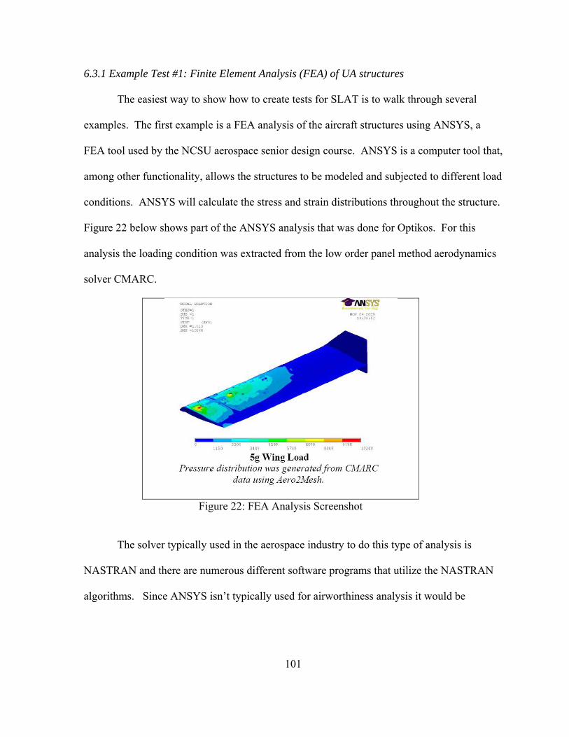
101

6.3.1 Example Test #1: Finite Element Analysis (FEA) of UA structures

The easiest way to show how to create tests for SLAT is to walk through several

examples. The first example is a FEA analysis of the aircraft structures using ANSYS, a

FEA tool used by the NCSU aerospace senior design course. ANSYS is a computer tool that,

among other functionality, allows the structures to be modeled and subjected to different load

conditions. ANSYS will calculate the stress and strain distributions throughout the structure.

Figure 22 below shows part of the ANSYS analysis that was done for Optikos. For this

analysis the loading condition was extracted from the low order panel method aerodynamics

solver CMARC.

 

Figure 22: FEA Analysis Screenshot

The solver typically used in the aerospace industry to do this type of analysis is

NASTRAN and there are numerous different software programs that utilize the NASTRAN

algorithms. Since ANSYS isn’t typically used for airworthiness analysis it would be

102

considered to fall into the “Less Than Manned Equivalent” category for the Verification

Method variable in the point allocation algorithm (reference back to Figure 8 for the full

algorithm). All five of the senior design aircraft are designed with a 1.5 factor of safety, the

standard for manned aircraft, and thus the Standard variable would be rated as “Manned

Equivalent.” The combination of the Manned Equivalent Standard and the Less Than

Manned Equivalent Verification method results in a quality scaling factor of 0.7 (from the

table in figure 8). This test fulfills the Analysis slot22. The next step in computing the points

for this example is to determine what failure modes are addressed by the FEA of the aircraft

structures. Table 14 below shows the compilation of the different relevant failure modes

from the tailored FMECA. Since all of the example aircraft have effectively the same

Structures Domain FMECA the values for this test can be used to illustrate how their relative

complexities change the points awarded.

22 As discussed earlier each failure mode can only contribute points via two tests: one Analytical and one Physical testing. 

103

Table 14: Failure Modes Addressed by FEA Test Structures Test 1 

Point Effects Description: 

Finite Element Analysis of full structures using 1.5 safety margin.  Done with ANSYS. 

Category:  Analysis  1 

Standard:  Manned Equivalent 0.7 

Verification Method:  Less than Manned Equivalent 

Max Criticality:  1‐ Catastrophic Failure Modes Addressed  Criticality 

Fuselage    

ST‐FS‐5: Bulkheads separate from other members (Poor Design)  3 ‐ Major 

ST‐FS‐10: Bulkheads rupture from impact (Poor Design)  3 ‐ Major 

ST‐FS‐15: Non‐compromising cracks in bulkheads (Poor Design)  4 ‐ Minor 

ST‐FS‐20: Delamination of Bulkhead Layers (Poor Design)  3 ‐ Major 

ST‐FS‐25: Other structural members buckle under load (Poor Design)  3 ‐ Major 

ST‐FS‐30: Other structural members separate (Poor Design)  3 ‐ Major 

Lifting Surface    

ST‐LS‐1: Main spar buckles under load (Poor Design)  1‐ Catastrophic 

ST‐LS‐6: Main spar failure due to material fatigue (Poor Design)  1‐ Catastrophic 

ST‐LS‐10: Ribs buckle under load (Poor Design)  2 ‐ Critical 

ST‐LS‐15: Ribs fail due to material fatigue (Poor Design)  2 ‐ Critical 

ST‐LS‐25: Ribs separate from main spar (Poor Design)  2 ‐ Critical 

ST‐LS‐30: Other structural members buckle under load (Poor Design)  2 ‐ Critical 

ST‐LS‐35: Other structural members fail due to material fatigue (Poor Design)  3 ‐ Major 

ST‐LS‐40: Wing joint fails in flight (Poor Design)  1‐ Catastrophic 

Skin    

ST‐SK‐1: Wing develops holes/cracks in Skin (Poor Design)  3 ‐ Major 

ST‐SK‐7: Wing skin delamination (Poor Design)  2 ‐ Critical 

ST‐SK‐13: Wing skin buckles under load (Poor Design)  2 ‐ Critical 

ST‐SK‐18: Wing skin dent/ding (Poor Design)  4 ‐ Minor 

ST‐SK‐24: Fuselage skin develops cracks/holes (Poor Design)  3 ‐ Major 

ST‐SK‐30: Fuselage skin delamination (Poor Design)  3 ‐ Major 

ST‐SK‐36: Fuselage skin buckles under load (Poor Design)  3 ‐ Major 

ST‐SK‐36: Fuselage skin dent/ding (Poor Design)  4 ‐ Minor 

Test Totals 

Catastrophic Failure Modes:  3  Major Failure Modes:  10 

Critical Failure Modes:  6  Minor Failures:  3 

104

Table 14 shows that the common thread in the addressed failure modes is the Poor

Design causal factor, which follows since this is a design phase analysis of the structures.

This test says nothing about the quality control of the manufacturing process, for instance, so

there would be no points granted toward addressing manufacturing defects.

As shown in the last two rows of Table 13 the FEA analysis addresses 3 Catastrophic,

6 Critical, 10 Major, and 3 Minor Failures. Even though the same number of failure modes

are being addressed, the amount of points awarded to the different aircraft varies depending

on their relative complexities. Aircraft with fewer Catastrophic and Critical failure modes

are granted more points for the FEA test because it covers proportionally more of the

important failure modes. Table 15 below shows the maximum number of points available for

the same FEA test based on the different aircraft complexities.

Table 15: Point Totals for FEA of Structures (Structures Test 1) 

   Goose   Hyperion 

   RC  Autopilot  RC Autopilot 

Max Possible Points: 217 217 114  114  Piolin  Optikos  Phoenix  

RC  Autopilot  RC  Autopilot  RC Autopilot 

Max Possible Points:  110  110 130 130 130  130

The table above shows that the FEA analysis of the structures for Optikos would be

worth a maximum of 130 points, but that is before the grader makes an assessment of the

quality of the test. The grader may only give 85% credit resulting in the UAS only getting

110 points for the FEA test. This demonstrates that a UAS doesn’t get the full points unless

the artifact shows that they fully addressed all of the failure modes. A grader might reduce

105

the points granted because of how the engineers approached meshing or constraining the

model or if grader felt that some key loading condition was ignored. It is expected that in the

actual implementation of this tool that the graders would be able to provide comments as to

why they docked points and have some path for developers to redo tests to improve their

scores. Most likely the grading will be done based on a set of guidelines and rubrics

established by the CA to help ensure that the grading is fair and consistent across different

platforms.

6.3.2 Example Test #2: Physical Load Test of Wing

As an example of physical testing versus the analytical test shown in Example #1 the

next test is designed based on the physical load test of the manufactured wing that must be

completed by the NCSU aerospace engineering students prior to first flight. Since the teams

are producing only one or two aircraft on a very short time frame (one semester to build and

fly their aircraft) it isn’t feasible to test a wing to failure (the manned standard)23. Instead the

flight article wings are tested up to the limit load with stain gauge instrumentation to

correlate actual strain values to those predicted in the design phase ANSYS analysis. The

loads are typically applied with bags of lead for the maximum load case. Figure 23 below

shows the wing load test of Optikos. The wing is suspended upside down and loaded with

bags of lead at twelve spanwise locations to simulate a +3 G loading. Strain gages are 23 There have been several wings that have failed during this load tests.  In the case of Phoenix it was due to an error in modeling the compressive strength of the foam core of the wing.  In another case the failure was due to a manufacturing defect where the spar cap had been cut near the root.  In both cases the wings were unloaded at the first sign of failure and the structures were repaired.  Both repaired wings were subjected to the load test again and had to pass in order to be deemed flight worthy. 

106

measuring the skin strains near the root of the wing and students are measuring the wing tip

deflections. Both the strains and wingtip deflections are compared to the expected values

from the FEA modeling.

 

Figure 23: Physical Wing Load test of flight wing

This test is “Less than Manned Equivalent” for both the standard and the verification

method24 so the quality rating is only 0.5, but since it is physically testing a manufactured

wing it receives double points. Table 16 below shows the detailed calculation of the points

for the wing loading test for all 5 example aircraft. This shows how physical testing of the

aircraft wing has captured many of the manufacturing defect failure modes not captured by

the FEA analysis.

24 A manned equivalent verification method would be using hydraulic actuators to apply the forces and the manned equivalent standard would be to take the load to 115% of the limit load and insure no permanent structural deformation and then take the load up to failure to show it meets the 1.5 factor of safety. 

Lead weights are placed at twelve spanwise locations

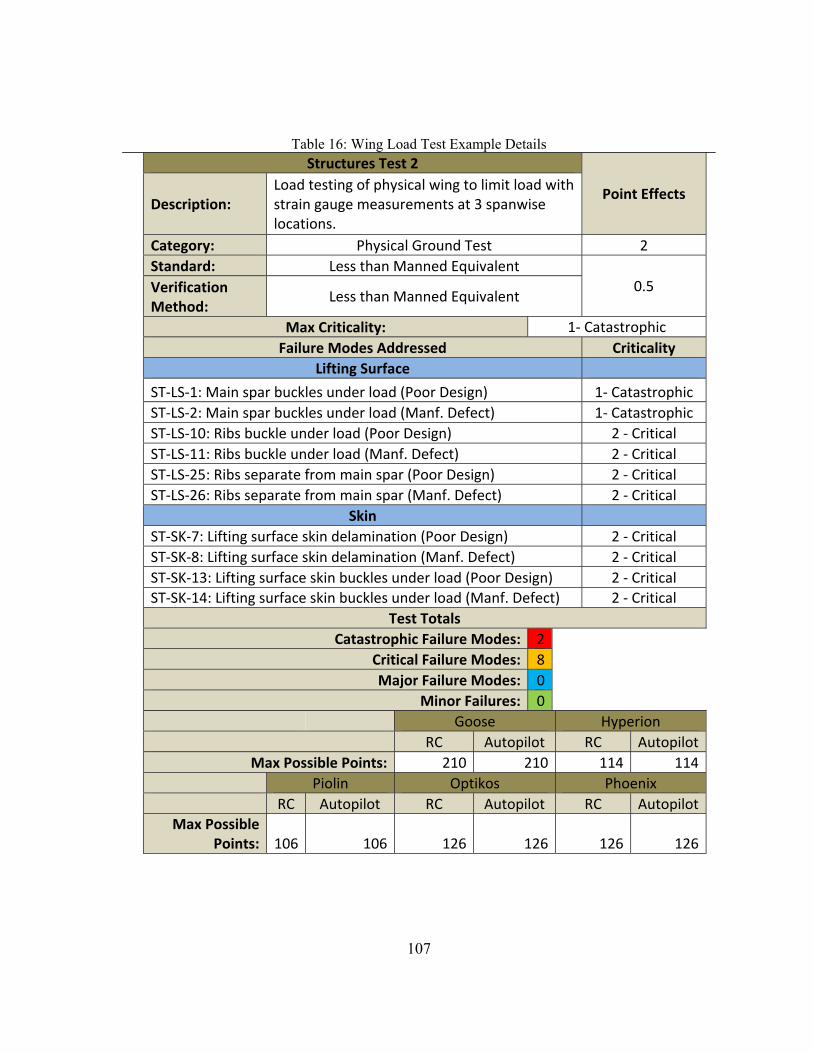
107

Table 16: Wing Load Test Example Details Structures Test 2 

Point Effects Description: 

Load testing of physical wing to limit load with strain gauge measurements at 3 spanwise locations. 

Category:  Physical Ground Test  2 Standard:  Less than Manned Equivalent 

0.5 Verification Method: 

Less than Manned Equivalent 

Max Criticality:  1‐ Catastrophic Failure Modes Addressed  Criticality 

Lifting Surface    

ST‐LS‐1: Main spar buckles under load (Poor Design)  1‐ Catastrophic ST‐LS‐2: Main spar buckles under load (Manf. Defect)  1‐ Catastrophic ST‐LS‐10: Ribs buckle under load (Poor Design)   2 ‐ Critical ST‐LS‐11: Ribs buckle under load (Manf. Defect)  2 ‐ Critical ST‐LS‐25: Ribs separate from main spar (Poor Design)  2 ‐ Critical ST‐LS‐26: Ribs separate from main spar (Manf. Defect)  2 ‐ Critical 

Skin    ST‐SK‐7: Lifting surface skin delamination (Poor Design)  2 ‐ Critical ST‐SK‐8: Lifting surface skin delamination (Manf. Defect)  2 ‐ Critical ST‐SK‐13: Lifting surface skin buckles under load (Poor Design)  2 ‐ Critical ST‐SK‐14: Lifting surface skin buckles under load (Manf. Defect)  2 ‐ Critical 

Test Totals Catastrophic Failure Modes: 2

Critical Failure Modes: 8Major Failure Modes: 0

Minor Failures: 0     Goose   Hyperion 

   RC  Autopilot  RC  AutopilotMax Possible Points: 210 210 114  114

  Piolin  Optikos  Phoenix   RC  Autopilot  RC  Autopilot  RC  Autopilot

Max Possible Points:  106  106 126 126 126  126

108

6.3.3 Example Test #3: Flight Test

Flight testing presents several difficulties when it comes to creating tests within

SLAT. The primary difficultly is that since flight testing involves the entire system the

testing will bridge many, if not all, domains. It is important that tests that cover more than

one domain should be created as a suite of tests.

To illustrate this principle the initial flights will be viewed as a set of flight tests

bundled into a single artifact. NC State Flight Research always conducts several proof-of-

flight tests of every senior design aircraft prior to allowing them to fly at picnic. This help to

ensure that the aircraft handling characteristics are well known and well behaved before they

are flown in a setting where more people are at risk.

The domain by domain details for this test are quite lengthy and can be found in

Appendix B. Determining the results of such tests can be quite tedious, but Table 17 below

shows the overall maximum points granted by the initial flight tests for Optikos, which will

be the aircraft used in most of the examples for the rest of this document.

Table 17: Compiled Flight Test Points for Optikos

Domain  R/C Config  Autopilot Added Structures  336  336 Propulsion  1243  1243 Electrical  741  799 Control Systems   2286  202 System Safety  2109  999 

Note that there was effectively no change in the Structures, Propulsion, or Electrical

domains when the autopilot was added. This is due to the FMECA for those domains not

109

being affected by the addition of the autopilot. One advantage to SLAT’s approach to

tailoring FMECA sets is that an addition of some system or assembly will only require the

affected domains to be reanalyzed.

6.4 Difficulties in Test Creation

The previous examples show the base approach for designing tests in SLAT and

should be sufficient for most of the physical aspects of any UAS. There are several domains

where developing the tests is more difficult. Of primary concern in this aspect are the areas

of Maintenance, Software Certification and System Safety.

6.4.1 Maintenance

SLAT doesn’t separate maintenance out as a unique domain as is done in MIL-

HDBK-516B due to constraints imposed by the point allocation algorithm25. Every

component will eventually wear out and fail. A very well designed aircraft will be

thoroughly not airworthy if the proper maintenance procedures are not followed. The risk

associated with maintenance depends on the expected mission life of the system. A

component may be appropriate with very little maintenance concerns if the system is a

demonstrator that will only perform a couple of flights, but may be a poor choice for a

deployed military system expected to fly hundreds of missions a year. For creating tests for

maintenance items it is important to review the data source when determining which slot is a

25 The point allocation algorithm is heavily dependent on the number of catastrophic and critical failures scaled based on the relative domain complexities.  Because of this aspect of the algorithm calculating points for maintenance tests as a separate domain becomes overly complicated as the number of failure modes between the different domains can be vastly different. 

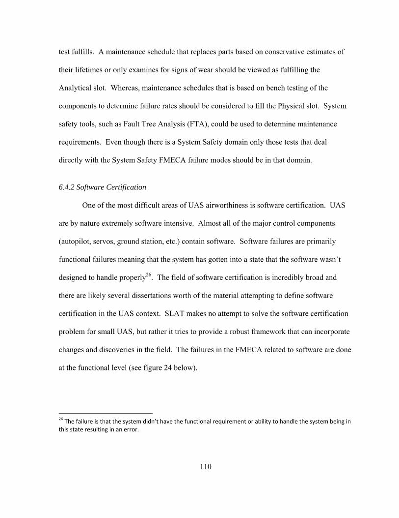
110

test fulfills. A maintenance schedule that replaces parts based on conservative estimates of

their lifetimes or only examines for signs of wear should be viewed as fulfilling the

Analytical slot. Whereas, maintenance schedules that is based on bench testing of the

components to determine failure rates should be considered to fill the Physical slot. System

safety tools, such as Fault Tree Analysis (FTA), could be used to determine maintenance

requirements. Even though there is a System Safety domain only those tests that deal

directly with the System Safety FMECA failure modes should be in that domain.

6.4.2 Software Certification

One of the most difficult areas of UAS airworthiness is software certification. UAS

are by nature extremely software intensive. Almost all of the major control components

(autopilot, servos, ground station, etc.) contain software. Software failures are primarily

functional failures meaning that the system has gotten into a state that the software wasn’t

designed to handle properly26. The field of software certification is incredibly broad and

there are likely several dissertations worth of the material attempting to define software

certification in the UAS context. SLAT makes no attempt to solve the software certification

problem for small UAS, but rather it tries to provide a robust framework that can incorporate

changes and discoveries in the field. The failures in the FMECA related to software are done

at the functional level (see figure 24 below).

26 The failure is that the system didn’t have the functional requirement or ability to handle the system being in this state resulting in an error. 

111

 

Figure 24: Autopilot Software FMECA selection (functional FMECA)

Any system that is software intensive will have a fundamentally different approach to

testing the software as opposed to testing the structures or propulsion system. Software

testing will likely be the application of a standard like DO-178B, which was developed for

certifying critical software for manned aircraft systems. Application of DO-178B would be

the only currently available manned equivalent standard and since DO-178B also defines the

target goals it also becomes the manned equivalent verification method. The application of

parts of DO-178B, such as Modified Condition/Decision Coverage ( MC/DC) testing27,

should be viewed as using the Less-than-Manned standard and verification method since it is

pulling only a piece of the certification process. Likewise, if some other software

certification process is used (perhaps one used in some other industry) it would be considered

Less-Than-Manned standard and verification method.

27 MC/DC testing is one of the more rigorous testing procedures done for flight critical aviation software.  It encompasses testing to show that all of the different system states for a section of code have been tested. 

112

The difference in Analysis versus Physical testing for software also requires some further

explanation. A flow diagram showing the program flow should be viewed as an Analysis

level test, while a test that showed that the actual software followed that flow diagram would

be a physical test. In general, any software artifact that deals with how the program was

design should be viewed as Analysis, while any artifact that shows what the code is doing

should be viewed as Physical28.

6.4.3 System Safety

System safety is another domain where the artifacts and testing will differ from those

typically thought of during airworthiness discussions. SLAT is primarily a system safety

tool. One of the popular airworthiness system safety tools, the FMECA process, forms the

basis for SLAT. It was decided to have the System Safety domain focus on the interfaces

between other parts of the system since those interfaces can be difficult to capture in standard

FMECA. In the base FMECA set for System Safety there are four sections:

• Autopilot Operator to External Pilot Interface

• Autopilot Operator to Vehicle Interface

• Ground Station Handover Interface

• Ground Crew Operations

28 The terminology “As Designed” and “As Written” are effective for making this distinction.  The hope is that following the software using some type of test harness would catch program errors where the code “as written” differs functionally from the code “as designed.”  Care must be taken to ensure that the “as designed” testing covers all of the needed functionality.  It is very easy to write code that behaves exactly as designed, but that design missed some key situations and still results in major software errors. 

113

The Autopilot Operator to External Pilot Interface focuses on the hand-off procedures

from the autopilot controlling the aircraft to some human physically controlling the aircraft.

This type of transition is typically done during the terminal phases of the mission. It is also

important to recognize that this transition can lead to numerous problems if either party isn’t

aware that control has been handed off. The Autopilot Operator to Vehicle Interface is

designed to capture many of the diagnostic and human factors issues that arise from remotely

operating a UAS. The Ground Station Handover Interface deals with handing control of a

UAS from one ground station to another ground station. It is important that positive control

be maintained during any of these transitions. The Ground Crew Operations FMECA really

captures the interface between the ground crew and the aircraft. The focus on this FMECA

are the SoF issues that are present whenever one is working around an aircraft, such as

encountering a spinning propeller, exposure to dangerous noise levels, etc.

Analysis slot tests for these failure modes are fairly easy to create and typically involve

application of system safety tools (FTA, Hazard Analysis, etc.). A simple Preliminary

Hazard Analysis of the flight line and ground crew would be a basic Analysis test. This

could be expanded by creating proper checklists and operational flow charts that help

separate the ground crew from potential threats. Another approach would be designing out

threats, such as being able to remotely start an aircraft’s engine so the ground crew is not

near the propeller when it is spinning29.

29 This example would actually be captured partially in the FMECA since being able to remotely start your aircraft engine in flight would likely change some of your failure mode criticalities.  The System Safety test component would be as part of something like a PHA showing that the hazard of contact with spinning propeller had been mitigated through design.   

114

Unfortunately, conducting physical tests for these interface failure modes can be very

difficult. It is expected that most of the physical testing would occur with inspections of

actual operational flow by a safety professional to determine if the hazard analysis had

missed anything.

6.5 SLAT Examples

This section shows the application of SLAT for the five example aircraft in both the

RC only and Autopilot Added configurations. The four example missions are the same for

all aircraft and configurations. These examples use the CDR documents produced as part of

the senior design as the majority of the artifacts30. Appendix A has the base points for each

aircraft in each configuration and Appendix B contains the details for all of the tests used in

this examples.

6.5.1 RC Configuration - Optikos

The flights conducted as part of the aerospace engineering senior project are done

using only a remote pilot. Due to budget and time constraints there is no autopilot on-board,

but an Eagletree data logger does provide some simple telemetry feedback. The flight line

has the primary pilot, a safety pilot, and a scribe. The primary pilot is responsible for the

flight and is considered the pilot in control. The safety pilot can take over the piloting

30 The CDR documents for all five aircraft should be distributed with this report for reference.  If not included please contact Dave Burke (dave.a.burke@gmail.com) and he can provide them. 

115

responsibility if needed31. The scribe takes notes about the flight, maintains the engine run-

time watch, and acts as communication relay. There is occasionally a fourth person

monitoring the telemetry downlink from the EagleTree to provide the pilot with airspeed data

if needed. These examples will examine the testing that was done for Optikos during the

senior design course to determine if they meet the TLS for the different missions.

Tables 18 through 22 below shows an example of the tests done prior to first flight for

Optikos to reach the TLS for a controlled flight (Unpopulated Region) at Perkins Field.

Table 18: Full Example of SLAT – Structures Domain

Structures Domain

Test Test Criticality Max Pts Grade Final Grades

FEA Software, full structures Catastrophic 130 45% 58

Load test of wing Catastrophic 126 50% 63

Launcher Performance Analysis Critical 21 Crit.

Req. Crit. Req.

Launcher Testing Critical 42 Crit. Req. Crit. Req.

First Flight Readiness Review Catastrophic 336 50% 168

Total for Structures Domain: 289

31 This has occurred once when an insect flew in between the primary pilot’s sunglasses and eye.  The primary pilot was able to hand control to the safety pilot, remove the insect, and take back control of the aircraft. 

116

Table 19: Full Example of SLAT – Propulsion Domain

Propulsion Domain

Test Test Criticality Max Pts Grade Final Grades

Motocalc Analysis Major 130 Crit. Req. Crit. Req.

Wind Tunnel Testing Catastrophic 776 65% 504

Static Testing Catastrophic 21 N/A N/A

Total for Propulsion Domain: 504

Table 20: Full Example of SLAT – Electrical Domain

Electrical Domain

Test Test Criticality Max Pts Grade Final Grades

Wiring Diagram Catastrophic 285 10% 28

First Flight Readiness Review Catastrophic 494 25% 123

Total for Electrical Domain: 151

117

Table 21: Full Example of SLAT – Control System Domain

Control System Domain

Test Test Criticality Max Pts Grade Final Grades

Handling Qualities Analysis Catastrophic 83 75% 62

Range Check of R/C Equipment Catastrophic 1215 35% 425

Paint Scheme Verification Catastrophic 59 20% 11

Total For Control System Domain: 498

Table 22: Full Example of SLAT – System Safety Domain

System Safety Domain

Test Test Criticality Max Pts Grade Final Grades

Checklists/Work flow for flight test Catastrophic 148 30% 44

Total for System Safety Domain: 44

118

 

Figure 25: SLAT Full Example, Optikos Prior to First Flight

Figure 25 shows that after the application of SLAT the System Safety domain has

enough points for a controlled flight test at Perkins Field, but not enough to fly at picnic.

Therefore, some initial flight tests are needed to get to the picnic TLS. Table 23 below

shows the results of the initial flight tests and Figure 26 shows the state of SLAT for Optikos

after those points are awarded.

0

100

200

300

400

500

600

Structures Propulsion Electrical Control System

System Safety

Optikos Prior to First Flight

TLS‐FF

TLS‐Picnic

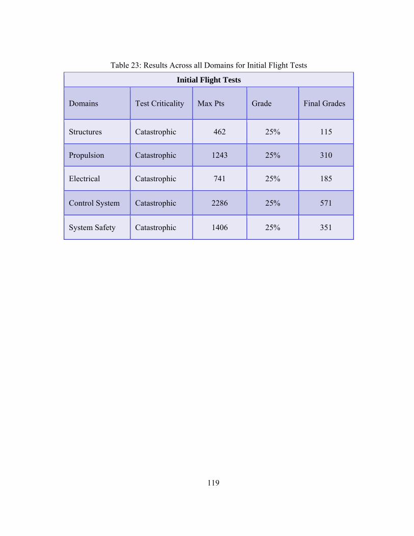
119

Table 23: Results Across all Domains for Initial Flight Tests

Initial Flight Tests

Domains Test Criticality Max Pts Grade Final Grades

Structures Catastrophic 462 25% 115

Propulsion Catastrophic 1243 25% 310

Electrical Catastrophic 741 25% 185

Control System Catastrophic 2286 25% 571

System Safety Catastrophic 1406 25% 351

120

Figure 26: Optikos SLAT after Initial Flight Tests

Figure 26 shows how the initial flight tests were able to raise all of the domains, but

particularly System Safety, such that all of the domains are now above the TLS to fly at

picnic.

6.5.2 Autopilot Added Configuration The next step is to examine what happens when the UAS configuration is changed.

For this example a generic autopilot is added to Optikos to make it capable of autonomous

flight. The addition of the autopilot adds failure modes to the Control System and System

Safety domains, requires the addition of the Ground Station domain, and changes the

complexities for the Electrical domain. These changes result in a reevaluation of the tests for

those domains. Now that there are significantly more high priority failure modes in those

domains the amount of points granted for addressing each one is reduced. Figure 24 below

shows the results of the previously discussed tests with the new failure modes from adding an

autopilot.

0

200

400

600

800

1000

1200

Structures Propulsion Electrical Control System

System Safety

Optikos After Initial Flights

TLS‐FF

TLS‐Picnic

121

Figure 27: After Autopilot Added

Figure 27 shows how the previous tests for Control System are now much less

valued. They now barely reach the TLS for a controlled flight at Butner. The more

important item is the addition of the Ground Station domain. No tests had been done

previously to address any of the failure modes of the ground station so that domain has zero

points. This means that the addition of the autopilot has made it necessary to go back to

either Analysis or Ground Testing levels to accumulate at least enough points to fly in the

controlled environment at Perkins Field.

0

100

200

300

400

500

600

700

800

900

Structures Propulsion Electrical Control System

System Safety

Ground Station

Optikos Autopilot Added

TLS‐FF

TLS‐Picnic

122

Chapter 7

Conclusion

Summary

SLAT addresses the challenges posed by certifying the airworthiness of fixed-wing

UAS between 2 lb. and 350 lb. MTOW by providing a flexible tool that CA could use as part

of the certification process, while also making the tool accessible to industry project

managers to help them design aircraft with certification in mind. SLAT is the first ever point

based approach to airworthiness (for manned or unmanned aircraft) and is the first tool to

specifically address the paradigm shift in airworthiness that is posed by unmanned systems.

The lower limit of 2 lb. is based on collecting and combing research on lethal KE

thresholds for blunt injuries. As such SLAT assumes that any UAS above 2 lb. is capable of

causing life threatening injuries to anyone struck during an uncontrolled crash of the vehicle.

SLAT’s use of a tailored FMECA for each UAS allows it to encapsulate the unique

aspects of any aircraft configuration and it is this flexibility that allows SLAT to handle the

vast variety of aircraft found in the small UAS category. The FMECA tailoring effectively

self-selects the airworthiness criteria that need to be addressed, while the algorithm for

allocating points for different types of tests allows the standards and verification methods to

vary below manned equivalent levels. SLAT leverages the subject matter experts that

already exist in the CA offices to provide solid oversight of the algorithms and lend their

experience and knowledge to the certification process. Points are granted on a domain by

123

domain basis as UAS developers show good engineering analysis, ground testing, and flight

testing artifacts.

The TLS that all the domains must reach is defined such that the certification

requirements will be commensurate with the threat posed by the aircraft to the people in the

mission area. All of the domains must meet the required TLS since a UAS is only as safe as

its weakest domain. The TLS and thus the airworthiness requirements are high for larger

vehicles flying over densely populated areas and reduce as the size of the aircraft and the

population densities of the mission area reduce. The research done during the development

of SLAT shows that four simple population density categories can be defined by utilizing the

marked urban areas on the sectional maps. This provides a simple method for mission

planning that allows for easy calculation of the exposed population put at risk by any

particular flight scenario.

Flexibility

SLAT is not a finalized tool, but rather it is a framework that is designed to be

modified and adjusted to meet differing CA and project management needs. All of the

algorithms in SLAT can be adjusted to better reflect specifics on a certain region (such as

providing more points for E3 ground tests than flight tests). One of the strengths in SLAT is

the ability to adjust these algorithms as more data and research becomes available for

evaluating specific contexts. Foundational Requirements can be established to properly

define specific cases or the scope of application. These Foundational Requirements can

124

ensure that SLAT conforms to expected requirements that may exist outside the variables

quantified by the different algorithms.

Future Work

There are a number of assumptions that had to be made during the development of

SLAT that could benefit from more direct investigation. The crash lethality and population

density components were addressed in detail, but some of the other assumptions were simply

beyond the scope of this initial research effort. These can be roughly categorized as

“Algorithm Components” and “Standards and Verification Components”.

Future Work – Algorithm Components

One area of future research would be the point weighting values the three levels of

testing. SLAT recognizes that in most of the standard airworthiness process flight testing is

the gold standard followed by ground testing of physical components and finally by

analytical means. To reflect this ranking flight tests get three times the number of points

compared to analytical means and ground tests get twice as many points as analytical means.

Although this ranking holds true for many of the domains there are certainly areas where this

ranking may not be the most appropriate choice. One area like this would be EMI testing of

components. Any testing done in a facility where the UAS can be placed into a highly

controlled electromagnetic environment will be far superior to the discontinuous data from

flight testing. In this case it may be more appropriate to weigh the points for ground testing

higher or even replace the “flight test” category with controlled “EMI facility.” Exactly what

125

scaling would be appropriate would need to be examined on a domain by domain basis. It is

even possible to change the point allocation algorithm such that the sum of the three

weightings is different than six, but the algorithm would need to be adjusted accordingly.

Another area for future research would be the relative weightings between Manned

and Less-than-Manned standards and verification methods. Currently there is a matrix that

reflects an initial evaluation of the different weightings. Further research could validate

those weightings or propose new weight matrices that better encapsulate the confidence lost

by reducing the standards and verification methods below the manned levels. For instance,

work could be performed that examined the relative value of using a 1.5 factor of safety on

flight critical structural components compared to a 1.3 factor of safety. There are numerous

areas in each domain where such analysis could be done to better determine the specific

weighting matrices.

Future Work – Standards and Verification Methods

One area that has a significant room for further research is the development of

specific standards and verification methods for items that are specific to the UAS context.

There are numerous UAS items that don’t exist in the manned aviation context, such as hand

launching handling characteristics. In the base design of SLAT those areas can only earn the

lower amount of points because there is no manned equivalent standard or verification

method. There are several groups (ASTM F-38 or RTCA SC-203 for instance) that are

currently investigating and developing such standards.

126

References [1]

Clothier, Reece A. “Determination and Evaluation of UAV Safety Objectives,” In Proceedings 21st International Unmanned Air Vehicle Systems Conference, Bristol, United Kingdom, 2006, pp 18.1-18.16.

[2] “STANAG 4671 – Unmanned Aerial Vehicle Systems Airworthiness

Requirements (USAR)”, Edition 1. NATO Document. 03 September 2009.

[3] MIL-HDBK-516B, “Airworthiness Certification Criteria.” U.S.A. Dept. of Defense. 26 September 2005.

[4] Title 14 of the United States of America Code of Federal Regulations. Federal

Aviation Regulations.

[5]

Jackson, Scott. Systems Engineering for Commercial Aircraft. Ashgate Publishing Ltd. 1997.

[6]

Murtha, Justin F., “An Evidence Theoretic Approach to Design of Reliable Low-Cost UAVs.” Masters Thesis. Virginia Polytechnic Institute and State University. Department of Aerospace and Ocean Engineering. 2009.

[7] The Office of the Secretary of Defense. “Unmanned Aircraft Systems Roadmap

2005-2030.”

[8]

De Florio, Filippo. Airworthiness: An Introduction to Aircraft Certification. A Guide to Understanding JAA, EASA, and FAA Standards. Butterworth-Heinimann 2006.

[9] Rodrigues, Clarence C.; Wells, Alexander T. “Commercial Aviation Safety. 4th

Edition”. McGraw-Hill. 2003.

[10] JAA Website, History Section. http://www.jaa.nl/introduction/introduction.html#top (cited 1 Feb 2010)

[11] ICAO Website, History Section.

http://www.icao.int/icao/en/howworks.htm (cited 1 February 2010)

[12] “Certification Specifications for Normal, Utility, Aerobatic, and Commuter, Category Aeroplanes”, EASA CS-23, November 2003.

[13] European Aviation Safety Agency (EASA), "Policy Statement Airworthiness

Certification of Unmanned Aircraft Systems (UAS)". 2009

127

[14]

Federal Aviation Administration. Aviation Safety, Unmanned Aircraft Program Office (AIR-160). “Interim Operational Approval Guidance 08-01. Unmanned Aircraft Systems Operations in the U. S. National Airspace System.” March 13, 2008

[15]

Federal Aviation Administration. Proposed Rulemaking from Small Unmanned Aircraft System Aviation Rulemaking Committee. “Comprehensive Set of Recommendations for sUAS Regulatory Development.” April 1, 2009

[16] MIT ICAT Website

http://web.mit.edu/aeroastro/labs/icat/ (cited Feb 13, 2010)

[17]

Weibel, Roland E.; Hansman, John R., “Safety Considerations for Operations of Unmanned Aerial Vehicles in the National Airspace System”. MIT International Center for Air Transportation. Report No. ICAT-2005-1. March 2005.

[18] Range Commanders Council (RCC) Standard 323-99 "Range Safety Criteria for

Unmanned Air Vehicles”. U.S.A Dept. of Defense. 2007 RCC-323-99

[19]

Cobleigh, Brent. “2007 Ikhana Western States and Southern California Emergency UAS Fire Missions,” NASA Document Report Server (ntrs.nasa.gov), document ID: 20080017326 [cited November 2009].

[20]

Federal Aviation Administration (FAA). Statutory Instruments – 2005 No. 1110 – Civil Aviation “The Rules of the Air (Amendment) Regulations 2005.” 1 April 2005

[21] Federal Register / Vol. 66, No. 60. Part IV Department of Commerce – Bureau

of the Census. 28 March 2001.

[22]

Range Commanders Council (RCC) Standard 321-07 “Common Risk Criteria Standards for National Test Ranges: Supplement”. U.S.A Dept. of Defense. 2007

[23] FAA Advisory Circular (AC) 431.35-1, “Expected Casualty Calculations for

Commercial Space Launch and Re-Entry Missions.” 30 August 2000.

[24] UVS International. “UAS – Unmanned Aircraft Systems. The Global Perspective 2007/2008.” Imprimerie Nouvelle. Normandy, France. 2007.

128

[25] The Joint JAA/EUROCONTROL Initiative on UAVs, “UAV Task Force: Final Report.” 11 May 2004.

[26]

Clare, Victor R.; Lewis, James H.; Mickiewicz, Alexander P.; Sturdivan, Larry M. “Blunt Trauma Data Correlation.” Edgewood Arsenal. EB-TR-75016. May 1976.

[27]

Lyon, David H.; Bir, Cynthia A.; Patton, Brendon J. ARL-TR-1868, “Injury Evaluation Techniques for Non-Lethal Kinetic Energy Munitions.” Army Research Lab. U.S.A. Dept. of Defense. January 1999.

[28]

Evans, David H. Probability and Its Applications for Engineers. ASQC Quality Press, Milwaukee. 1992

[29] Stamatis, D.H. “Failure Mode and Effect Analysis: FMEA from Theory to

Execution. 2nd Edition”, ASQ Quality Press, 2003

[30]

Weibel, Roland E., “Safety Considerations for Operations of Unmanned Aerial Vehicles in the National Airspace System”. Masters Thesis. Massachusetts Institute of Technology, Department of Aeronautics and Astronautics. 2005

129

APPENDICES

130

Appendix A:  

Failure Counts and Base Point Calculations

Total Failures for Example UAS Between Both Configurations

RC Configuration Autopilot Added Configuration

Optikos 482 690 Phoenix 632 840 Piolin 614 822 Goose 985 1,193 Hyperion 1135 1,343

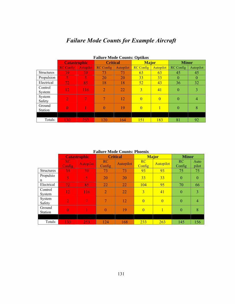
131

Failure Mode Counts for Example Aircraft

Failure Mode Counts: Optikos

Catastrophic Critical Major Minor RC Config Autopilot RC Config Autopilot RC Config Autopilot RC Config Autopilot

Structures 39 39 73 73 63 63 45 45 Propulsion 5 5 20 20 33 33 0 0 Electrical 72 85 18 18 52 43 36 32 Control System 12 116 2 22 3 41 0 3 System Safety 2 7 7 12 0 0 0 4 Ground Station 0 1 0 19 0 1 0 8

Totals: 130 253 120 164 151 183 81 92

Failure Mode Counts: Phoenix Catastrophic Critical Major Minor

RC Config Autopilot RC

Config Autopilot RC Config Autopilot RC

Config Autopilot

Structures 39 39 73 73 93 93 75 75 Propulsion 5 5 20 20 33 33 0 0 Electrical 72 85 22 22 104 95 70 66 Control System 12 116 2 22 3 41 0 3 System Safety 2 7 7 12 0 0 0 4 Ground Station 0 1 0 19 0 1 0 8

Totals: 130 253 124 168 233 263 145 156

132

Failure Mode Counts: Piolin Catastrophic Critical Major Minor

RC Config Autopilot RC

Config Autopilot RC Config Autopilot RC

Config Autopi

lot Structures 54 54 78 78 75 75 55 55 Propulsion 5 5 20 20 33 33 0 0 Electrical 95 108 25 25 87 78 61 57 Control System 12 116 2 22 3 41 0 3 System Safety 2 7 7 12 0 0 0 4 Ground Station 0 1 0 19 0 1 0 8

Totals: 168 291 132 176 198 228 116 127

Failure Mode Counts: Goose Catastrophic Critical Major Minor

RC Config Autopilot RC

Config Autopilot RC Config Autopilot RC

Config Autopilot

Structures 9 9 57 57 192 192 160 160 Propulsion 6 6 32 32 46 46 16 16 Electrical 26 39 24 24 242 233 156 152 Control System 12 116 2 22 3 41 0 3 System Safety 2 7 7 12 0 0 0 4 Ground Station 0 1 0 19 0 1 0 8

Totals: 55 178 122 166 483 513 332 343

133

Failure Mode Counts: Hyperion Catastrophic Critical Major Minor

RC Config Autopilot RC

Config Autopilot RC Config Autopilot RC

Config Autopilot

Structures 39 39 87 87 192 192 160 160 Propulsion 6 6 32 32 46 46 16 16 Electrical 72 85 34 34 260 251 172 168 Control System 12 116 2 22 3 41 0 3 System Safety 2 7 7 12 0 0 0 4 Ground Station 0 1 0 19 0 1 0 8

Totals: 131 254 162 206 501 531 348 359

134

Base Points for Example Aircraft

Base Points: Optikos

Catastrophic Critical Major Minor

RC Config Autopilot RC

Config Autopilot RC Config Autopilot RC

Config Autopilot

Structures 15 15 12 12 6 6 3 3 Propulsion 67 67 53 53 27 27 13 13 Electrical 19 16 15 13 7 6 4 3 Control System 119 12 95 10 48 5 24 2 System Safety 185 88 148 70 74 35 37 18 Ground Station N/A 83 N/A 67 N/A 33 N/A 17

Base Points: Phoenix Catastrophic Critical Major Minor

RC Config Autopilot RC

Config Autopilot RC Config Autopilot RC

Config Autopilot

Structures 15 15 12 12 6 6 3 3 Propulsion 67 67 53 53 27 27 13 12 Electrical 18 16 14 12 7 6 4 3 Control System 119 12 95 10 48 5 24 2 System Safety 185 88 148 70 74 35 37 18 Ground Station N/A 83 N/A 67 N/A 33 N/A 17

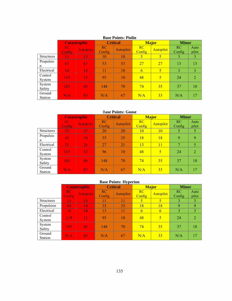
135

Base Points: Piolin Catastrophic Critical Major Minor

RC Config Autopilot RC

Config Autopilot RC Config Autopilot RC

Config Autopilot

Structures 13 13 10 10 5 5 3 3 Propulsion 67 67 53 53 27 27 13 13 Electrical 14 13 11 10 6 5 3 3 Control System 119 12 95 10 48 5 24 2 System Safety 185 88 148 70 74 35 37 18 Ground Station N/A 83 N/A 67 N/A 33 N/A 17

Base Points: Goose Catastrophic Critical Major Minor

RC Config Autopilot RC

Config Autopilot RC Config Autopilot RC

Config Autopilot

Structures 25 25 20 20 10 10 5 5 Propulsion 44 44 35 35 18 18 9 9 Electrical 33 26 27 21 13 11 7 5 Control System 119 12 96 10 48 5 24 2 System Safety 185 88 148 70 74 35 37 18 Ground Station N/A 83 N/A 67 N/A 33 N/A 17

Base Points: Hyperion

Catastrophic Critical Major Minor

RC Config Autopilot RC

Config Autopilot RC Config Autopilot RC

Config Autopilot

Structures 13 13 11 11 5 5 3 3 Propulsion 44 44 35 35 18 18 9 9 Electrical 16 14 13 11 6 6 3 3 Control System 119 12 95 10 48 5 24 2 System Safety 185 88 148 70 74 35 37 18 Ground Station N/A 83 N/A 67 N/A 33 N/A 17

136

Appendix B:  

Point Allocation for Example Tests

This Appendix includes the formulation and point allocation calculation for all of the tests used for in the example applications of SLAT. For all five aircraft the base tests are the same

although the Points granted for each test vary depending on aircraft configuration and complexity.

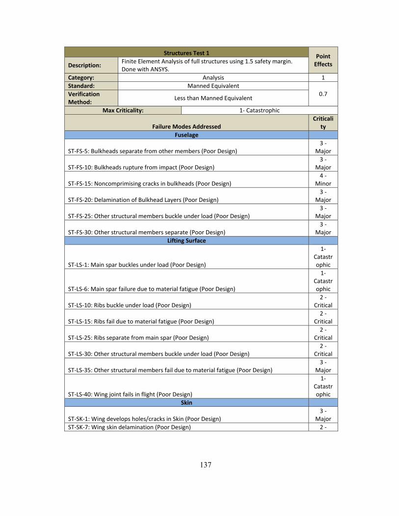
137

Structures Test 1  Point Effects Description: 

Finite Element Analysis of full structures using 1.5 safety margin.  Done with ANSYS. 

Category:  Analysis 1Standard:  Manned Equivalent

0.7 Verification Method: 

Less than Manned Equivalent 

Max Criticality:  1‐ Catastrophic

Failure Modes Addressed Criticali

ty Fuselage

ST‐FS‐5: Bulkheads separate from other members (Poor Design) 3 ‐

Major 

ST‐FS‐10: Bulkheads rupture from impact (Poor Design) 3 ‐

Major 

ST‐FS‐15: Noncomprimising cracks in bulkheads (Poor Design) 4 ‐

Minor 

ST‐FS‐20: Delamination of Bulkhead Layers (Poor Design) 3 ‐

Major 

ST‐FS‐25: Other structural members buckle under load (Poor Design) 3 ‐

Major 

ST‐FS‐30: Other structural members separate (Poor Design) 3 ‐

Major Lifting Surface

ST‐LS‐1: Main spar buckles under load (Poor Design) 

1‐Catastrophic 

ST‐LS‐6: Main spar failure due to material fatigue (Poor Design) 

1‐Catastrophic 

ST‐LS‐10: Ribs buckle under load (Poor Design) 2 ‐

Critical 

ST‐LS‐15: Ribs fail due to material fatigue (Poor Design) 2 ‐

Critical 

ST‐LS‐25: Ribs separate from main spar (Poor Design) 2 ‐

Critical 

ST‐LS‐30: Other structural members buckle under load (Poor Design) 2 ‐

Critical 

ST‐LS‐35: Other structural members fail due to material fatigue (Poor Design) 3 ‐

Major 

ST‐LS‐40: Wing joint fails in flight (Poor Design) 

1‐Catastrophic 

Skin

ST‐SK‐1: Wing develops holes/cracks in Skin (Poor Design) 3 ‐

Major ST‐SK‐7: Wing skin delamination (Poor Design) 2 ‐

138

Critical

ST‐SK‐13: Wing skin buckles under load (Poor Design) 2 ‐

Critical 

ST‐SK‐18: Wing skin dent/ding (Poor Design) 4 ‐

Minor 

ST‐SK‐24: Fuselage skin develops cracks/holes (Poor Design) 3 ‐

Major 

ST‐SK‐30: Fuselage skin delamination (Poor Design) 3 ‐

Major 

ST‐SK‐36: Fuselage skin buckles under load (Poor Design) 3 ‐

Major 

ST‐SK‐36: Fuselage skin dent/ding (Poor Design) 4 ‐

Minor Test Totals

Catastrophic Failure Modes: 3Critical Failure Modes: 6Major Failure Modes: 10

Minor Failures: 3   Goose  Hyperion 

   RC  Autopilot  RC Autopil

ot Max Possible Points: 217 217 114  114

  Piolin  Optikos Phoenix  

RC  Autopilot  RC  Autopilot  RC Autopil

ot Max 

Points:  110  110  130  130  130  130 

139

Structures Test 2 Point Effects 

Description: Load testing of physical wing to limit load with strain gauge measurements at 3 spanwise locations. 

Category:  Physical Ground Test 2 Standard:  Less than Manned Equivalent

0.5 Verification Method: 

Less than Manned Equivalent 

Max Criticality: 1‐ Catastrophic Failure Modes Addressed Criticality

Lifting Surface   ST‐LS‐1: Main spar buckles under load (Poor Design) 1‐ CatastrophicST‐LS‐2: Main spar buckles under load (Manf. Defect) 1‐ CatastrophicST‐LS‐10: Ribs buckle under load (Poor Design)  2 ‐ CriticalST‐LS‐11: Ribs buckle under load (Manf. Defect) 2 ‐ CriticalST‐LS‐25: Ribs separate from main spar (Poor Design) 2 ‐ CriticalST‐LS‐26: Ribs separate from main spar (Manf. Defect) 2 ‐ Critical

Skin   ST‐SK‐7: Lifting surface skin delamination (Poor Design) 2 ‐ CriticalST‐SK‐8: Lifting surface skin delamination (Manf. Defect) 2 ‐ CriticalST‐SK‐13: Lifting surface skin buckles under load (Poor Design) 2 ‐ CriticalST‐SK‐14: Lifting surface skin buckles under load (Manf. Defect) 2 ‐ Critical

Test TotalsCatastrophic Failure Modes: 2

Critical Failure Modes: 8Major Failure Modes: 0

Minor Failures: 0   Goose  Hyperion 

   RC Autopilot RC  AutopilotMax Possible Points: 210 210 114  114

  Piolin  Optikos Phoenix   RC  Autopilot RC Autopilot RC  Autopilot

Max Possible Points:  106  106  126  126  126  126 

140

Structures Test 3Point Effects 

Description: Analysis of Launcher Performance: includes both release profiles and structural analysis of launcher 

Category:  Analysis 1Standard:  Less than Manned Equivalent

0.5 Verification Method: 

Less than Manned Equivalent 

Max Criticality: 2 ‐ CriticalFailure Modes Addressed Criticality

Launcher   ST‐LN‐1: Launcher legs collapse while vehicle attached (Poor Design) 4 ‐ MinorST‐LN‐3: Launcher legs collapse during launch (Poor Design) 2 ‐ CriticalST‐LN‐8: Aircraft improperly separates from launcher during launch (Poor Design of cradle  2 ‐ Critical ST‐LN‐13: Release mechanism fails to trigger on command (Poor Design) 4 ‐ MinorST‐LN‐16: Uncommanded release of trigger mechanism (Poor Design) 2 ‐ Critical

Test TotalsCatastrophic Failure Modes: 0

Critical Failure Modes: 3Major Failure Modes: 0

Minor Failures: 2   Goose  Hyperion

   RC Autopilot RC  AutopilotMax Possible Points: N/A N/A N/A  N/A

  Piolin Optikos Phoenix  RC  Autopilot RC Autopilot RC  Autopilot

Max Possible Points:  18  18  21  21  130  130 

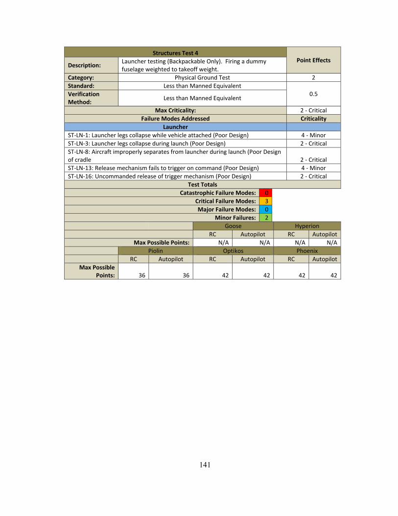
141

Structures Test 4 Point Effects 

Description: Launcher testing (Backpackable Only).  Firing a dummy fuselage weighted to takeoff weight. 

Category:  Physical Ground Test 2 Standard:  Less than Manned Equivalent

0.5 Verification Method: 

Less than Manned Equivalent 

Max Criticality: 2 ‐ CriticalFailure Modes Addressed Criticality

Launcher   ST‐LN‐1: Launcher legs collapse while vehicle attached (Poor Design) 4 ‐ MinorST‐LN‐3: Launcher legs collapse during launch (Poor Design) 2 ‐ CriticalST‐LN‐8: Aircraft improperly separates from launcher during launch (Poor Design of cradle  2 ‐ Critical ST‐LN‐13: Release mechanism fails to trigger on command (Poor Design) 4 ‐ MinorST‐LN‐16: Uncommanded release of trigger mechanism (Poor Design) 2 ‐ Critical

Test TotalsCatastrophic Failure Modes: 0

Critical Failure Modes: 3Major Failure Modes: 0

Minor Failures: 2   Goose  Hyperion 

   RC Autopilot RC  AutopilotMax Possible Points: N/A N/A N/A  N/A

  Piolin Optikos Phoenix   RC  Autopilot RC Autopilot RC  Autopilot

Max Possible Points:  36  36  42  42  42  42 

142

Structures Test 5Point Effects 

Description:  Landing Gear Analysis (Jets only)Category:  Analysis 1Standard:  Less than Manned Equivalent

0.5 Verification Method:  Less than Manned Equivalent

Max Criticality: 2 ‐ CriticalFailure Modes Addressed Criticality

Landing SystemST‐LG‐1: Landing gear bent/deformed on landing(Poor Design) 3 ‐ MajorST‐LG‐7: Landing gear fracture on landing(Poor Design) 2 ‐ CriticalST‐LG‐13: Landing gear wheel sticks during landing (Poor Design) 2 ‐ CriticalST‐LG‐19: Landing gear wheel bent/deformed permanently during landing (Poor Design)  3 ‐ MajorST‐LG‐25: Landing gear wheel fractures during landing (Poor Design) 2 ‐ CriticalST‐LG‐31: Landing gear tire fails during landing (Poor Design) 2 ‐ Critical

Test TotalsCatastrophic Failure Modes: 0 

Critical Failure Modes: 4 Major Failure Modes: 2 

Minor Failures: 0    Goose  Hyperion

   RC Autopilot RC  AutopilotMax Possible Points: 50 50  27  27

  Piolin Optikos Phoenix  RC  Autopilot RC Autopilot RC  Autopilot

Max Possible Points:  N/A  N/A  N/A  N/A  N/A  N/A 

143

Structures Test 6Point Effects 

Description:  Landing Gear Drop Test (Jets only)Category:  Analysis 1Standard:  Less than Manned Equivalent

0.5 Verification Method: 

Less than Manned Equivalent 

Max Criticality: 2 ‐ Critical Failure Modes Addressed Criticality

ST‐LG‐1: Landing gear bent/deformed on landing(Poor Design) 3 ‐MajorST‐LG‐2: Landing gear bent/deformed on landing (Manf. Defect) 3 ‐MajorST‐LG‐7: Landing gear fracture on landing(Poor Design) 2 ‐ CriticalST‐LG‐8: Landing gear fracture on landing (Manf. Defect) 2 ‐ CriticalST‐LG‐13: Landing gear wheel sticks during landing (Poor Design) 2 ‐ CriticalST‐LG‐14: Landing gear wheel sticks during landing (Manf. Defect) 2 ‐ CriticalST‐LG‐19: Landing gear wheel bent/deformed permanently during landing (Poor Design)  3 ‐MajorST‐LG‐20: Landing gear wheel bent/deformed permanently during landing (Manf. Defect)  3 ‐MajorST‐LG‐25: Landing gear wheel fractures during landing (Poor Design) 2 ‐ CriticalST‐LG‐26: Landing gear wheel fractures during landing (Manf. Defect) 2 ‐ CriticalST‐LG‐31: Landing gear tire fails during landing (Poor Design) 2 ‐ CriticalST‐LG‐32: Landing gear tire fails during landing (Manf. Defect) 2 ‐ Critical

Test TotalsCatastrophic Failure Modes: 0 

Critical Failure Modes: 8 Major Failure Modes: 4 

Minor Failures: 0    Goose  Hyperion

   RC Autopilot RC  AutopilotMax Possible Points: 100 100  54  54

  Piolin Optikos Phoenix  RC  Autopilot RC Autopilot RC  Autopilot

Max Possible Points:  N/A  N/A  N/A  N/A  N/A  N/A 

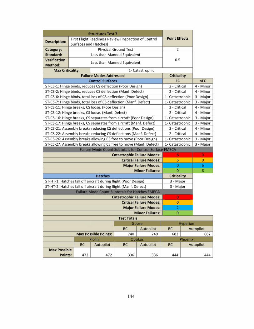
144

Structures Test 7 Point Effects 

Description: First Flight Readiness Review (Inspection of Control Surfaces and Hatches) 

Category:  Physical Ground Test 2 Standard:  Less than Manned Equivalent

0.5 Verification Method: 

Less than Manned Equivalent 

Max Criticality:  1‐ CatastrophicFailure Modes Addressed Criticality 

Control Surfaces FC  nFCST‐CS‐1: Hinge binds, reduces CS deflection (Poor Design) 2 ‐ Critical  4 ‐ MinorST‐CS‐2: Hinge binds, reduces CS deflection (Manf. Defect) 2 ‐ Critical  4 ‐ MinorST‐CS‐6: Hinge binds, total loss of CS deflection (Poor Design) 1‐ Catastrophic  3 ‐ MajorST‐CS‐7: Hinge binds, total loss of CS deflection (Manf. Defect) 1‐ Catastrophic  3 ‐ MajorST‐CS‐11: Hinge breaks, CS loose. (Poor Design) 2 ‐ Critical  4 ‐ MinorST‐CS‐12: Hinge breaks, CS loose. (Manf. Defect) 2 ‐ Critical  4 ‐ MinorST‐CS‐16: Hinge breaks, CS separates from aircraft (Poor Design) 1‐ Catastrophic  3 ‐ MajorST‐CS‐17: Hinge breaks, CS separates from aircraft (Manf. Defect) 1‐ Catastrophic  3 ‐ MajorST‐CS‐21: Assembly breaks reducing CS deflections (Poor Design) 2 ‐ Critical  4 ‐ MinorST‐CS‐22: Assembly breaks reducing CS deflections (Manf. Defect) 2 ‐ Critical  4 ‐ MinorST‐CS‐26: Assembly breaks allowing CS free to move (Poor Design) 1‐ Catastrophic  3 ‐ MajorST‐CS‐27: Assembly breaks allowing CS free to move (Manf. Defect) 1‐ Catastrophic  3 ‐ Major

Failure Mode Count Subtotals for Control Surface FMECACatastrophic Failure Modes: 6  0 

Critical Failure Modes: 6  0 Major Failure Modes: 0  6 

Minor Failures: 0  6 Hatches Criticality 

ST‐HT‐1: Hatches fall off aircraft during flight (Poor Design) 3 ‐Major ST‐HT‐2: Hatches fall off aircraft during flight (Manf. Defect) 3 ‐Major 

Failure Mode Count Subtotals for Hatches FMECACatastrophic Failure Modes: 0 

Critical Failure Modes: 0 Major Failure Modes: 2 

Minor Failures: 0 Test Totals

   Goose  Hyperion    RC Autopilot RC AutopilotMax Possible Points: 740 740 682  682

  Piolin  Optikos Phoenix   RC  Autopilot RC Autopilot RC Autopilot

Max Possible Points:  472  472  336  336  444  444 

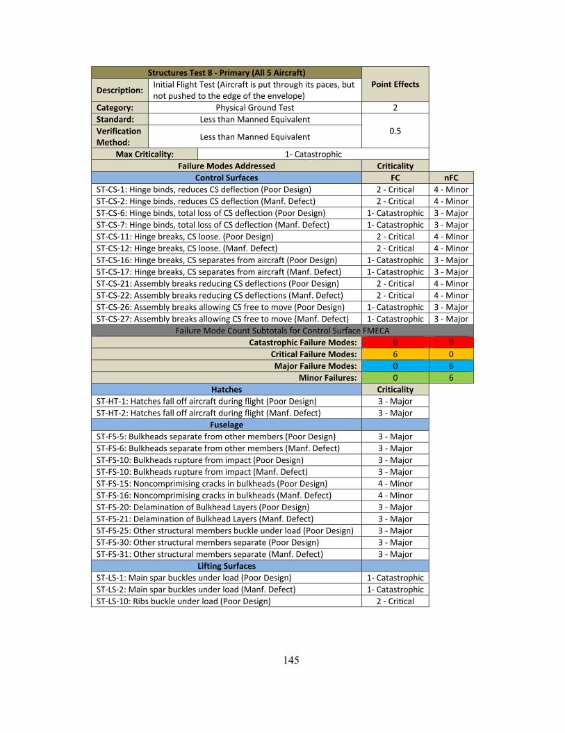
145

Structures Test 8 ‐ Primary (All 5 Aircraft)Point Effects 

Description: Initial Flight Test (Aircraft is put through its paces, but not pushed to the edge of the envelope) 

Category:  Physical Ground Test 2 Standard:  Less than Manned Equivalent

0.5 Verification Method: 

Less than Manned Equivalent 

Max Criticality:  1‐ CatastrophicFailure Modes Addressed Criticality 

Control Surfaces FC  nFCST‐CS‐1: Hinge binds, reduces CS deflection (Poor Design) 2 ‐ Critical  4 ‐ MinorST‐CS‐2: Hinge binds, reduces CS deflection (Manf. Defect) 2 ‐ Critical  4 ‐ MinorST‐CS‐6: Hinge binds, total loss of CS deflection (Poor Design) 1‐ Catastrophic  3 ‐ MajorST‐CS‐7: Hinge binds, total loss of CS deflection (Manf. Defect) 1‐ Catastrophic  3 ‐ MajorST‐CS‐11: Hinge breaks, CS loose. (Poor Design) 2 ‐ Critical  4 ‐ MinorST‐CS‐12: Hinge breaks, CS loose. (Manf. Defect) 2 ‐ Critical  4 ‐ MinorST‐CS‐16: Hinge breaks, CS separates from aircraft (Poor Design) 1‐ Catastrophic  3 ‐ MajorST‐CS‐17: Hinge breaks, CS separates from aircraft (Manf. Defect) 1‐ Catastrophic  3 ‐ MajorST‐CS‐21: Assembly breaks reducing CS deflections (Poor Design) 2 ‐ Critical  4 ‐ MinorST‐CS‐22: Assembly breaks reducing CS deflections (Manf. Defect) 2 ‐ Critical  4 ‐ MinorST‐CS‐26: Assembly breaks allowing CS free to move (Poor Design) 1‐ Catastrophic  3 ‐ MajorST‐CS‐27: Assembly breaks allowing CS free to move (Manf. Defect) 1‐ Catastrophic  3 ‐ Major

Failure Mode Count Subtotals for Control Surface FMECACatastrophic Failure Modes: 6  0 

Critical Failure Modes: 6  0 Major Failure Modes: 0  6 

Minor Failures: 0  6 Hatches Criticality 

ST‐HT‐1: Hatches fall off aircraft during flight (Poor Design) 3 ‐Major ST‐HT‐2: Hatches fall off aircraft during flight (Manf. Defect) 3 ‐Major 

FuselageST‐FS‐5: Bulkheads separate from other members (Poor Design) 3 ‐Major ST‐FS‐6: Bulkheads separate from other members (Manf. Defect) 3 ‐Major ST‐FS‐10: Bulkheads rupture from impact (Poor Design) 3 ‐Major ST‐FS‐10: Bulkheads rupture from impact (Manf. Defect) 3 ‐Major ST‐FS‐15: Noncomprimising cracks in bulkheads (Poor Design) 4 ‐Minor ST‐FS‐16: Noncomprimising cracks in bulkheads (Manf. Defect) 4 ‐Minor ST‐FS‐20: Delamination of Bulkhead Layers (Poor Design) 3 ‐Major ST‐FS‐21: Delamination of Bulkhead Layers (Manf. Defect) 3 ‐Major ST‐FS‐25: Other structural members buckle under load (Poor Design) 3 ‐Major ST‐FS‐30: Other structural members separate (Poor Design) 3 ‐Major ST‐FS‐31: Other structural members separate (Manf. Defect) 3 ‐Major 

Lifting SurfacesST‐LS‐1: Main spar buckles under load (Poor Design) 1‐ Catastrophic ST‐LS‐2: Main spar buckles under load (Manf. Defect) 1‐ Catastrophic ST‐LS‐10: Ribs buckle under load (Poor Design)  2 ‐ Critical 

146

ST‐LS‐11: Ribs buckle under load (Manf. Defect) 2 ‐ Critical ST‐LS‐25: Ribs separate from main spar (Poor Design) 2 ‐ Critical ST‐LS‐26: Ribs separate from main spar (Manf. Defect) 2 ‐ Critical ST‐LS‐40: Wing Joint fails in flight (Poor Design) 1‐ Catastrophic ST‐LS‐41: Wing Joint fails in flight (Manf. Defect) 1‐ Catastrophic 

SkinST‐SK‐7: Lifting surface skin delamination (Poor Design) 2 ‐ Critical ST‐SK‐8: Lifting surface skin delamination (Manf. Defect) 2 ‐ Critical ST‐SK‐13: Lifting surface skin buckles under load (Poor Design) 2 ‐ Critical ST‐SK‐14: Lifting surface skin buckles under load (Manf. Defect) 2 ‐ Critical 

Failure Mode Count Subtotals for Hatches FMECACatastrophic Failure Modes: 4 

Critical Failure Modes: 8 

Major Failure Modes:  11 Minor Failures: 2 

Test Totals   Goose  Hyperion 

   RC Autopilot RC AutopilotMax Possible Points: 740 740 682  682

  Piolin  Optikos Phoenix   RC  Autopilot RC Autopilot RC Autopilot

Max Possible Points:  472  472  336  336  444  444 

147

Propulsion Test 1 (Backpackable UAS Only)Point Effects 

Description: Motocalc analysis of propeller, motor, and ESC. 

Category:  Analysis 1Standard:  Less than Manned Equivalent

0.5 Verification Method:  Less than Manned Equivalent

Max Criticality: 3 ‐MajorFailure Modes Addressed Criticality 

Electric MotorPR‐EM‐22: Batteries insufficient (Poor Design) 3 ‐Major PR‐EM‐31: Motor Overheats (Poor Design) 3 ‐Major 

Test TotalsCatastrophic Failure Modes: 0

Critical Failure Modes: 0Major Failure Modes: 2

Minor Failures: 0   Goose  Hyperion

   RC Autopilot RC  AutopilotMax Possible Points: N/A N/A N/A  N/A

  Piolin Optikos Phoenix  RC  Autopilot RC Autopilot RC  Autopilot

Max Possible Points:  27  27  27  27  27  27 

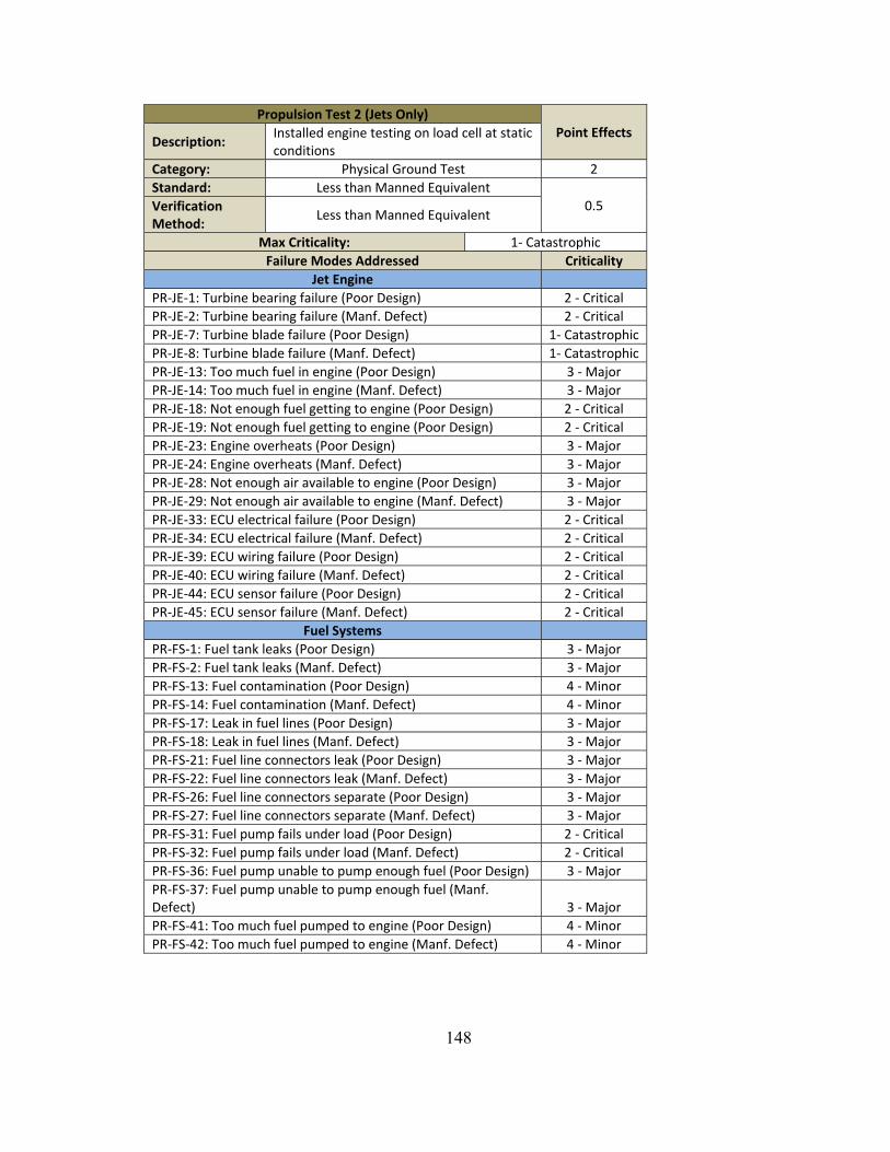
148

Propulsion Test 2 (Jets Only)Point Effects 

Description: Installed engine testing on load cell at static conditions 

Category:  Physical Ground Test 2Standard:  Less than Manned Equivalent

0.5 Verification Method: 

Less than Manned Equivalent 

Max Criticality:  1‐ CatastrophicFailure Modes Addressed Criticality

Jet EnginePR‐JE‐1: Turbine bearing failure (Poor Design) 2 ‐ CriticalPR‐JE‐2: Turbine bearing failure (Manf. Defect) 2 ‐ CriticalPR‐JE‐7: Turbine blade failure (Poor Design) 1‐ Catastrophic PR‐JE‐8: Turbine blade failure (Manf. Defect) 1‐ Catastrophic PR‐JE‐13: Too much fuel in engine (Poor Design) 3 ‐MajorPR‐JE‐14: Too much fuel in engine (Manf. Defect) 3 ‐MajorPR‐JE‐18: Not enough fuel getting to engine (Poor Design) 2 ‐ CriticalPR‐JE‐19: Not enough fuel getting to engine (Poor Design) 2 ‐ CriticalPR‐JE‐23: Engine overheats (Poor Design) 3 ‐MajorPR‐JE‐24: Engine overheats (Manf. Defect) 3 ‐MajorPR‐JE‐28: Not enough air available to engine (Poor Design) 3 ‐MajorPR‐JE‐29: Not enough air available to engine (Manf. Defect) 3 ‐MajorPR‐JE‐33: ECU electrical failure (Poor Design) 2 ‐ CriticalPR‐JE‐34: ECU electrical failure (Manf. Defect) 2 ‐ CriticalPR‐JE‐39: ECU wiring failure (Poor Design) 2 ‐ CriticalPR‐JE‐40: ECU wiring failure (Manf. Defect) 2 ‐ CriticalPR‐JE‐44: ECU sensor failure (Poor Design) 2 ‐ CriticalPR‐JE‐45: ECU sensor failure (Manf. Defect) 2 ‐ Critical

Fuel SystemsPR‐FS‐1: Fuel tank leaks (Poor Design) 3 ‐MajorPR‐FS‐2: Fuel tank leaks (Manf. Defect) 3 ‐MajorPR‐FS‐13: Fuel contamination (Poor Design) 4 ‐MinorPR‐FS‐14: Fuel contamination (Manf. Defect) 4 ‐MinorPR‐FS‐17: Leak in fuel lines (Poor Design) 3 ‐MajorPR‐FS‐18: Leak in fuel lines (Manf. Defect) 3 ‐MajorPR‐FS‐21: Fuel line connectors leak (Poor Design) 3 ‐MajorPR‐FS‐22: Fuel line connectors leak (Manf. Defect) 3 ‐MajorPR‐FS‐26: Fuel line connectors separate (Poor Design) 3 ‐MajorPR‐FS‐27: Fuel line connectors separate (Manf. Defect) 3 ‐MajorPR‐FS‐31: Fuel pump fails under load (Poor Design) 2 ‐ CriticalPR‐FS‐32: Fuel pump fails under load (Manf. Defect) 2 ‐ CriticalPR‐FS‐36: Fuel pump unable to pump enough fuel (Poor Design) 3 ‐MajorPR‐FS‐37: Fuel pump unable to pump enough fuel (Manf. Defect)  3 ‐ Major PR‐FS‐41: Too much fuel pumped to engine (Poor Design) 4 ‐MinorPR‐FS‐42: Too much fuel pumped to engine (Manf. Defect) 4 ‐Minor

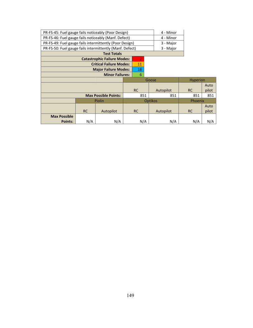
149

PR‐FS‐45: Fuel gauge fails noticeably (Poor Design) 4 ‐MinorPR‐FS‐46: Fuel gauge fails noticeably (Manf. Defect) 4 ‐MinorPR‐FS‐49: Fuel gauge fails intermittently (Poor Design) 3 ‐MajorPR‐FS‐50: Fuel gauge fails intermittently (Manf. Defect) 3 ‐Major

Test TotalsCatastrophic Failure Modes: 2

Critical Failure Modes: 11Major Failure Modes: 18

Minor Failures: 6   Goose  Hyperion

   RC  Autopilot  RC Autopilot 

Max Possible Points: 851 851 851  851  Piolin Optikos Phoenix 

RC  Autopilot  RC  Autopilot  RC Autopilot 

Max Possible Points:  N/A  N/A  N/A  N/A  N/A  N/A 

150

Propulsion Test 3 (Backpackable UAS Only) Point Effects 

Description: Wind tunnel testing of propulsion system throughout expected flight speeds. 

Category:  Physical Ground Test 2 Standard:  Less than Manned Equivalent

0.5 Verification Method:  Less than Manned Equivalent

Max Criticality: 1‐ Catastrophic Failure Modes Addressed Criticality 

Electric Motor   PR‐EM‐1: Motor mount fails and separates (Poor Design) 1‐ Catastrophic PR‐EM‐2: Motor mount fails and separates (Manf. Defect) 1‐ Catastrophic PR‐EM‐6: Motor mount breaks, motor loose (Poor Design) 2 ‐ Critical PR‐EM‐7: Motor mount breaks, motor loose (Manf. Defect) 2 ‐ Critical PR‐EM‐11: Motor mount bolts back out (Poor Design) 3 ‐ Major PR‐EM‐12: Motor mount bolts back out (Manf. Defect) 3 ‐ Major PR‐EM‐16: Motor mount bolts fail under load (Poor Design) 3 ‐ Major PR‐EM‐17: Motor mount bolts fail under load (Manf. Defect) 3 ‐ Major PR‐EM‐21: Batteries unable to supply needed load (Poor Design) 3 ‐ Major PR‐EM‐22: Batteries unable to supply needed load (Manf. Defect) 3 ‐ Major PR‐EM‐31: Motor overheats (Poor Design) 3 ‐ Major PR‐EM‐32: Motor overheats (Manf. Defect) 3 ‐ Major PR‐EM‐36: Motor stops working (Poor Design) 2 ‐ Critical PR‐EM‐37: Motor stops working (Manf. Defect) 2 ‐ Critical 

Propellers   PR‐PL‐1: Prop damaged (Poor Design) 3 ‐ Major PR‐PL‐2: Prop damaged (Manf. Defect) 3 ‐ Major PR‐PL‐7: Prop separates from aircraft (Poor Design) 2 ‐ Critical PR‐PL‐8: Prop separates from aircraft (Manf. Defect) 2 ‐ Critical PR‐PL‐12: Prop is unbalanced (Poor Design) 3 ‐ Major PR‐PL‐13: Prop is unbalanced (Manf. Defect) 3 ‐ Major 

Test Totals

Catastrophic Failure Modes:  2 

Critical Failure Modes:  6 

Major Failure Modes:  12 

Minor Failures:  0 

      Goose   Hyperion 

   RC  Autopilot  RC Autopil

ot 

Max Possible Points:  N/A  N/A  N/A  N/A   Piolin  Optikos  Phoenix   RC  Autopilot  RC  Autopilot  RC  Autopilot 

Max Possible Points:  776  776  776  776  776  776 

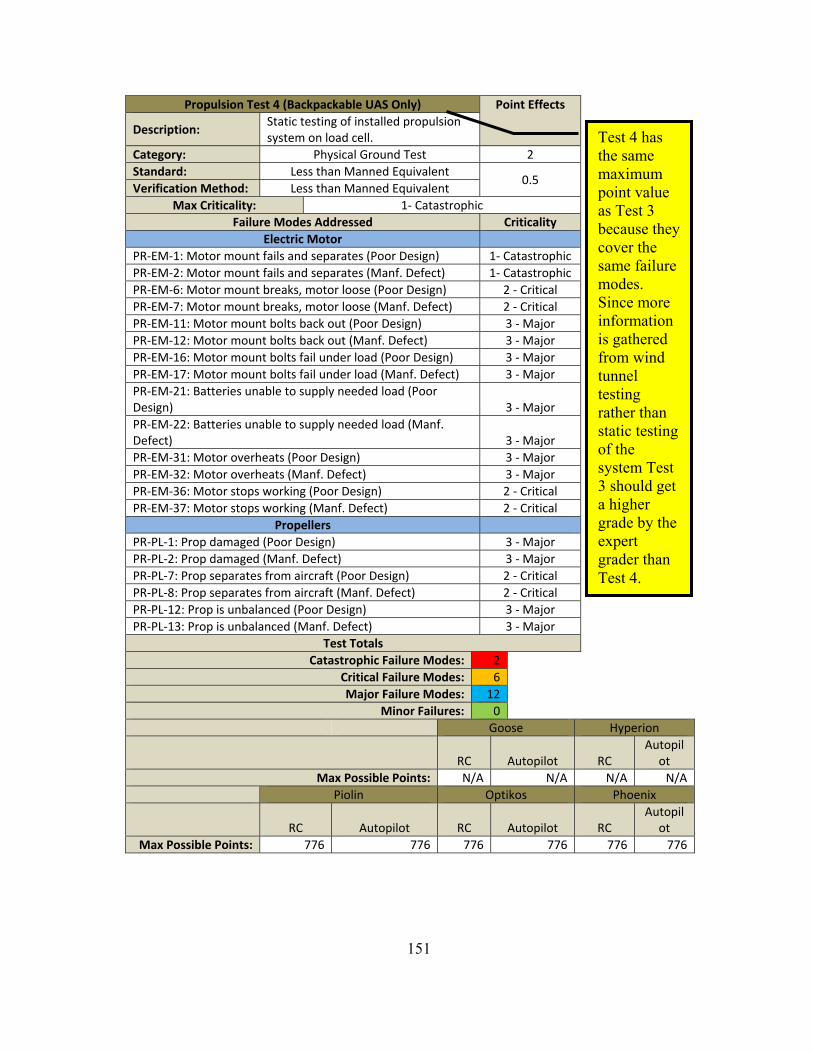
151

Propulsion Test 4 (Backpackable UAS Only) Point Effects

Description: Static testing of installed propulsion system on load cell. 

Category:  Physical Ground Test 2Standard:  Less than Manned Equivalent

0.5 Verification Method:  Less than Manned Equivalent

Max Criticality:  1‐ CatastrophicFailure Modes Addressed Criticality

Electric MotorPR‐EM‐1: Motor mount fails and separates (Poor Design) 1‐ Catastrophic PR‐EM‐2: Motor mount fails and separates (Manf. Defect) 1‐ Catastrophic PR‐EM‐6: Motor mount breaks, motor loose (Poor Design) 2 ‐ CriticalPR‐EM‐7: Motor mount breaks, motor loose (Manf. Defect) 2 ‐ CriticalPR‐EM‐11: Motor mount bolts back out (Poor Design) 3 ‐MajorPR‐EM‐12: Motor mount bolts back out (Manf. Defect) 3 ‐MajorPR‐EM‐16: Motor mount bolts fail under load (Poor Design) 3 ‐MajorPR‐EM‐17: Motor mount bolts fail under load (Manf. Defect) 3 ‐MajorPR‐EM‐21: Batteries unable to supply needed load (Poor Design)  3 ‐ Major PR‐EM‐22: Batteries unable to supply needed load (Manf. Defect)  3 ‐ Major PR‐EM‐31: Motor overheats (Poor Design) 3 ‐MajorPR‐EM‐32: Motor overheats (Manf. Defect) 3 ‐MajorPR‐EM‐36: Motor stops working (Poor Design) 2 ‐ CriticalPR‐EM‐37: Motor stops working (Manf. Defect) 2 ‐ Critical

PropellersPR‐PL‐1: Prop damaged (Poor Design) 3 ‐MajorPR‐PL‐2: Prop damaged (Manf. Defect) 3 ‐MajorPR‐PL‐7: Prop separates from aircraft (Poor Design) 2 ‐ CriticalPR‐PL‐8: Prop separates from aircraft (Manf. Defect) 2 ‐ CriticalPR‐PL‐12: Prop is unbalanced (Poor Design) 3 ‐MajorPR‐PL‐13: Prop is unbalanced (Manf. Defect) 3 ‐Major

Test TotalsCatastrophic Failure Modes: 2

Critical Failure Modes: 6Major Failure Modes: 12

Minor Failures: 0   Goose  Hyperion

   RC  Autopilot  RC Autopil

ot Max Possible Points: N/A N/A N/A  N/A

  Piolin Optikos Phoenix 

RC  Autopilot  RC  Autopilot  RC Autopil

ot Max Possible Points:  776  776 776 776 776  776

Test 4 has the same maximum point value as Test 3 because they cover the same failure modes. Since more information is gathered from wind tunnel testing rather than static testing of the system Test 3 should get a higher grade by the expert grader than Test 4.

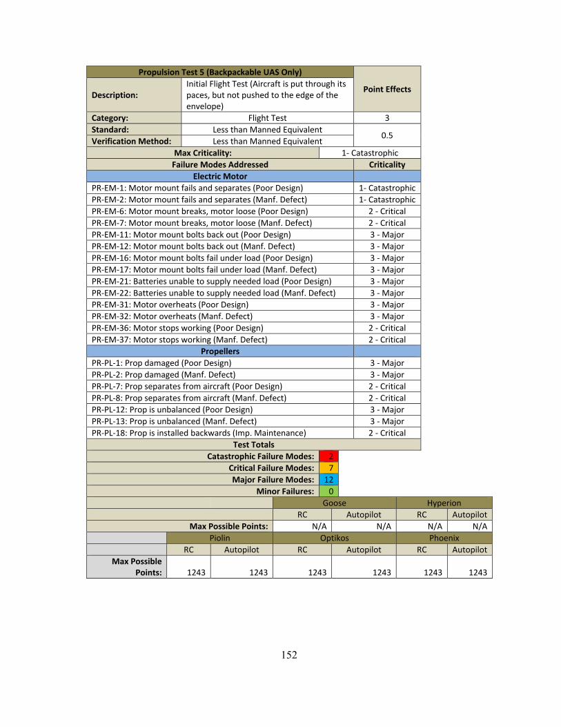
152

Propulsion Test 5 (Backpackable UAS Only)

Point Effects Description: 

Initial Flight Test (Aircraft is put through its paces, but not pushed to the edge of the envelope) 

Category:  Flight Test 3Standard:  Less than Manned Equivalent

0.5 Verification Method:  Less than Manned Equivalent

Max Criticality: 1‐ Catastrophic Failure Modes Addressed Criticality 

Electric MotorPR‐EM‐1: Motor mount fails and separates (Poor Design) 1‐ Catastrophic PR‐EM‐2: Motor mount fails and separates (Manf. Defect) 1‐ Catastrophic PR‐EM‐6: Motor mount breaks, motor loose (Poor Design) 2 ‐ Critical PR‐EM‐7: Motor mount breaks, motor loose (Manf. Defect) 2 ‐ Critical PR‐EM‐11: Motor mount bolts back out (Poor Design) 3 ‐Major PR‐EM‐12: Motor mount bolts back out (Manf. Defect) 3 ‐Major PR‐EM‐16: Motor mount bolts fail under load (Poor Design) 3 ‐Major PR‐EM‐17: Motor mount bolts fail under load (Manf. Defect) 3 ‐Major PR‐EM‐21: Batteries unable to supply needed load (Poor Design) 3 ‐Major PR‐EM‐22: Batteries unable to supply needed load (Manf. Defect) 3 ‐Major PR‐EM‐31: Motor overheats (Poor Design) 3 ‐Major PR‐EM‐32: Motor overheats (Manf. Defect) 3 ‐Major PR‐EM‐36: Motor stops working (Poor Design) 2 ‐ Critical PR‐EM‐37: Motor stops working (Manf. Defect) 2 ‐ Critical 

PropellersPR‐PL‐1: Prop damaged (Poor Design) 3 ‐Major PR‐PL‐2: Prop damaged (Manf. Defect) 3 ‐Major PR‐PL‐7: Prop separates from aircraft (Poor Design) 2 ‐ Critical PR‐PL‐8: Prop separates from aircraft (Manf. Defect) 2 ‐ Critical PR‐PL‐12: Prop is unbalanced (Poor Design) 3 ‐Major PR‐PL‐13: Prop is unbalanced (Manf. Defect) 3 ‐Major PR‐PL‐18: Prop is installed backwards (Imp. Maintenance) 2 ‐ Critical 

Test TotalsCatastrophic Failure Modes: 2

Critical Failure Modes: 7Major Failure Modes: 12

Minor Failures: 0   Goose  Hyperion

   RC Autopilot RC  AutopilotMax Possible Points: N/A N/A N/A  N/A

  Piolin Optikos Phoenix  RC  Autopilot RC Autopilot RC  Autopilot

Max Possible Points:  1243  1243  1243  1243  1243  1243 

153

Propulsion Test 6 (Jets Only)

Point Effects Description: 

Initial Flight Test (Aircraft is put through its paces, but not pushed to the edge of the envelope) 

Category:  Flight Test 3Standard:  Less than Manned Equivalent

0.5 Verification Method: 

Less than Manned Equivalent 

Max Criticality: 1‐ CatastrophicFailure Modes Addressed Criticality 

Jet EnginePR‐JE‐1: Turbine bearing failure (Poor Design) 2 ‐ Critical PR‐JE‐2: Turbine bearing failure (Manf. Defect) 2 ‐ Critical PR‐JE‐7: Turbine blade failure (Poor Design) 1‐ Catastrophic PR‐JE‐8: Turbine blade failure (Manf. Defect) 1‐ Catastrophic PR‐JE‐13: Too much fuel in engine (Poor Design) 3 ‐Major PR‐JE‐14: Too much fuel in engine (Manf. Defect) 3 ‐Major PR‐JE‐18: Not enough fuel getting to engine (Poor Design) 2 ‐ Critical PR‐JE‐19: Not enough fuel getting to engine (Poor Design) 2 ‐ Critical PR‐JE‐23: Engine overheats (Poor Design) 3 ‐Major PR‐JE‐24: Engine overheats (Manf. Defect) 3 ‐Major PR‐JE‐28: Not enough air available to engine (Poor Design) 3 ‐Major PR‐JE‐29: Not enough air available to engine (Manf. Defect) 3 ‐Major PR‐JE‐33: ECU electrical failure (Poor Design) 2 ‐ Critical PR‐JE‐34: ECU electrical failure (Manf. Defect) 2 ‐ Critical PR‐JE‐39: ECU wiring failure (Poor Design) 2 ‐ Critical PR‐JE‐40: ECU wiring failure (Manf. Defect) 2 ‐ Critical PR‐JE‐44: ECU sensor failure (Poor Design) 2 ‐ Critical PR‐JE‐45: ECU sensor failure (Manf. Defect) 2 ‐ Critical 

Fuel SystemsPR‐FS‐1: Fuel tank leaks (Poor Design) 3 ‐Major PR‐FS‐2: Fuel tank leaks (Manf. Defect) 3 ‐Major PR‐FS‐13: Fuel contamination (Poor Design) 4 ‐Minor PR‐FS‐14: Fuel contamination (Manf. Defect) 4 ‐Minor PR‐FS‐17: Leak in fuel lines (Poor Design) 3 ‐Major PR‐FS‐18: Leak in fuel lines (Manf. Defect) 3 ‐Major PR‐FS‐21: Fuel line connectors leak (Poor Design) 3 ‐Major PR‐FS‐22: Fuel line connectors leak (Manf. Defect) 3 ‐Major PR‐FS‐26: Fuel line connectors separate (Poor Design) 3 ‐Major PR‐FS‐27: Fuel line connectors separate (Manf. Defect) 3 ‐Major PR‐FS‐31: Fuel pump fails under load (Poor Design) 2 ‐ Critical PR‐FS‐32: Fuel pump fails under load (Manf. Defect) 2 ‐ Critical PR‐FS‐36: Fuel pump unable to pump enough fuel (Poor Design) 3 ‐Major PR‐FS‐37: Fuel pump unable to pump enough fuel (Manf. Defect) 3 ‐Major PR‐FS‐41: Too much fuel pumped to engine (Poor Design) 4 ‐Minor PR‐FS‐42: Too much fuel pumped to engine (Manf. Defect) 4 ‐Minor 

154

PR‐FS‐45: Fuel gauge fails noticeably (Poor Design) 4 ‐Minor PR‐FS‐46: Fuel gauge fails noticeably (Manf. Defect) 4 ‐Minor PR‐FS‐49: Fuel gauge fails intermittently (Poor Design) 3 ‐Major PR‐FS‐50: Fuel gauge fails intermittently (Manf. Defect) 3 ‐Major 

Test TotalsCatastrophic Failure Modes: 2

Critical Failure Modes: 12Major Failure Modes: 18

Minor Failures: 6   Goose  Hyperion

   RC Autopilot RC  AutopilotMax Possible Points: 1329 1329  1329  1329

  Piolin Optikos Phoenix  RC  Autopilot RC Autopilot RC  Autopilot

Max Possible Points:  N/A  N/A  N/A  N/A  N/A  N/A 

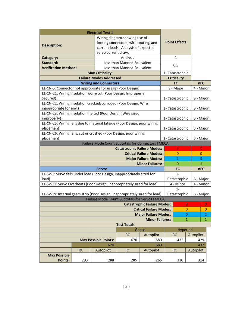
155

Electrical Test 1 

Point Effects Description: 

Wiring diagram showing use of locking connectors, wire routing, and current loads.  Analysis of expected servo current draw. 

Category:  Analysis 1 Standard:  Less than Manned Equivalent

0.5 Verification Method:  Less than Manned Equivalent

Max Criticality: 1‐ Catastrophic Failure Modes Addressed Criticality Wiring and Connectors FC  nFC

EL‐CN‐5: Connector not appropriate for usage (Poor Design) 3 ‐ Major  4 ‐MinorEL‐CN‐21: Wiring insulation worn/cut (Poor Design, Improperly Secured)  1‐ Catastrophic  3 ‐ Major EL‐CN‐22: Wiring insulation cracked/corroded (Poor Design, Wire inappropriate for env.)  1‐ Catastrophic  3 ‐ Major EL‐CN‐23: Wiring insulation melted (Poor Design, Wire sized improperly)  1‐ Catastrophic  3 ‐ Major EL‐CN‐25: Wiring fails due to material fatigue (Poor Design, poor wiring placement)  1‐ Catastrophic  3 ‐ Major EL‐CN‐26: Wiring fails, cut or crushed (Poor Design, poor wiring placement)  1‐ Catastrophic  3 ‐ Major 

Failure Mode Count Subtotals for Connectors FMECACatastrophic Failure Modes: 5  0

Critical Failure Modes: 0  0Major Failure Modes: 1  5

Minor Failures: 0  1Servos FC  nFC

EL‐SV‐1: Servo fails under load (Poor Design, inappropriately sized for load) 

1‐ Catastrophic  3 ‐ Major 

EL‐SV‐11: Servo Overheats (Poor Design, inappropriately sized for load) 4 ‐ Minor  4 ‐Minor

EL‐SV‐19: Internal gears strip (Poor Design, inappropriately sized for load) 1‐ 

Catastrophic  3 ‐ Major Failure Mode Count Subtotals for Servos FMECA

Catastrophic Failure Modes: 2  0Critical Failure Modes: 0  0Major Failure Modes: 0  2

Minor Failures: 1  1Test Totals

   Goose  Hyperion    RC Autopilot RC  AutopilotMax Possible Points: 670 589 432  429

  670 589 432  RC  Autopilot RC Autopilot RC  Autopilot

Max Possible Points:  293  288  285  266  330  314 

156

Electrical Test 2

Point Effects Description: 

First Flight Readiness Review ‐ Electrical Check Out Test.  This test goes through all the electrical components ensuring that they are working properly, the wires are properly routed, and properly connected.  This includes setting the servo deflections for the radio system. 

Category:  Physical Ground Test 2 Standard:  Less than Manned Equivalent

0.5 Verification Method: 

Less than Manned Equivalent 

Max Criticality: 1‐ Catastrophic 

Failure Modes Addressed  Criticality Wiring & Connectors  FC  nFC 

EL‐CN‐1: Poor connection between wires (Improper Maintenance)  1‐ Catastrophic 3 ‐

Major 

EL‐CN‐2: Poor connection between wires (Manf. Defect)  1‐ Catastrophic 3 ‐

Major 

EL‐CN‐3: Short in connector (Poor Design)  1‐ Catastrophic 

2 ‐Critica

l 

EL‐CN‐5: Connector damaged (Poor Design, not appropriate for use)  1‐ Catastrophic 

2 ‐Critica

l 

EL‐CN‐9: Connector inserted improperly (Poor Design, no key)  2 ‐ Critical 3 ‐

Major EL‐CN‐10: Connector inserted improperly or wrong connection (Poorly Labeled)  2 ‐ Critical 

3 ‐Major 

Failure Mode Count Subtotals for Connectors FMECACatastrophic Failure Modes: 4  0

Critical Failure Modes: 2  2Major Failure Modes: 0  4

Minor Failures: 0  0Servos FC  nFC

EL‐SV‐1: Servo fails during test (Poor Design)  1‐ Catastrophic 3 ‐

Major 

EL‐SV‐2: Servo fails during test (Manf. Defect)  1‐ Catastrophic 3 ‐

Major EL‐SV‐6: Servo goes to uncommanded position (Poor Design, low quality)  3 ‐ Major 

4 ‐Minor 

EL‐SV‐7: Servo goes to uncommanded position (Manf. Defect, bad servo)  3 ‐ Major 4 ‐

Minor 

EL‐SV‐9: Servo goes to uncommanded position (EMI)  3 ‐ Major 4 ‐

Minor 

EL‐SV‐12: Servo overheats (Manf. Defect, bad servo)  3 ‐ Major 4 ‐

Minor 

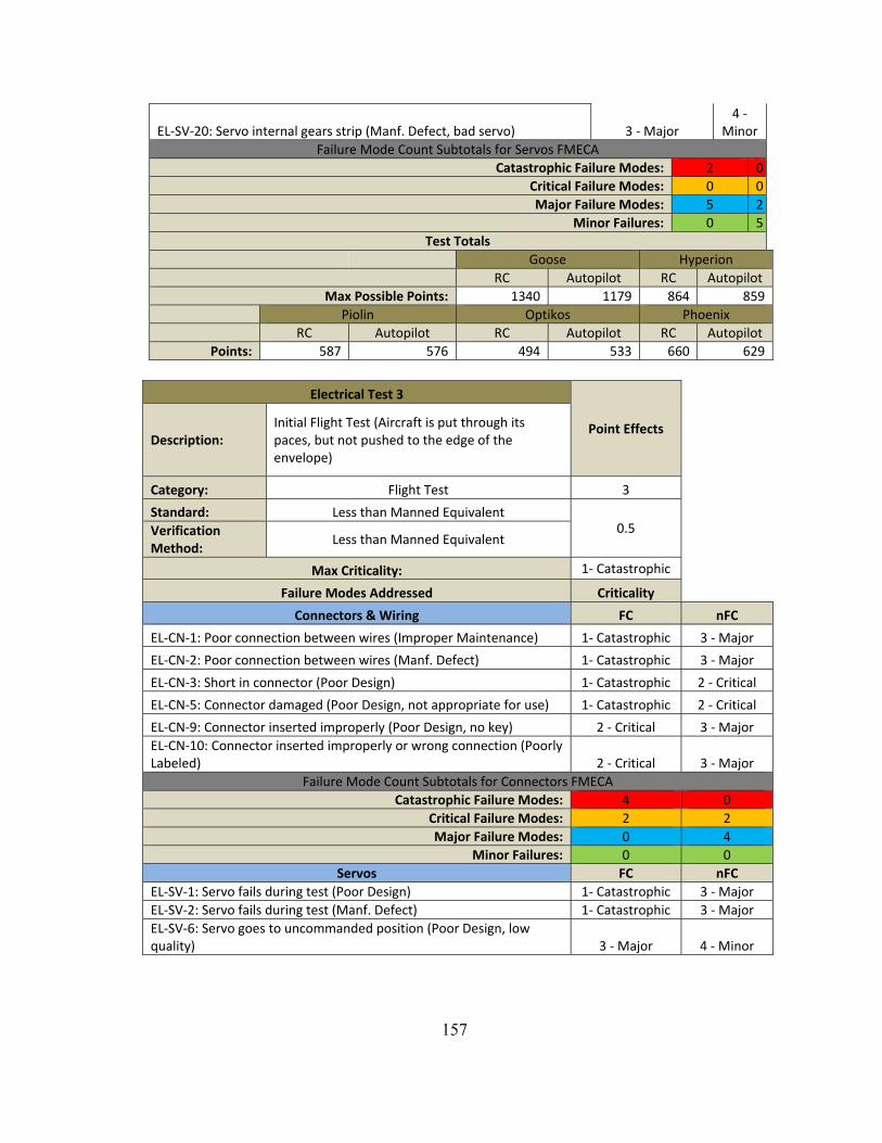
157

EL‐SV‐20: Servo internal gears strip (Manf. Defect, bad servo)  3 ‐ Major 4 ‐

Minor Failure Mode Count Subtotals for Servos FMECA

Catastrophic Failure Modes:  2 0Critical Failure Modes:  0 0Major Failure Modes:  5 2

Minor Failures:  0 5Test Totals

   Goose  Hyperion   RC Autopilot  RC  Autopilot

Max Possible Points: 1340 1179  864  859  Piolin Optikos Phoenix  RC  Autopilot RC Autopilot  RC  AutopilotPoints:  587  576 494 533  660  629

Electrical Test 3 

Point Effects Description: 

Initial Flight Test (Aircraft is put through its paces, but not pushed to the edge of the envelope) 

Category:  Flight Test  3 

Standard:  Less than Manned Equivalent 0.5 Verification 

Method: Less than Manned Equivalent 

Max Criticality:  1‐ Catastrophic 

Failure Modes Addressed  Criticality 

Connectors & Wiring  FC  nFC 

EL‐CN‐1: Poor connection between wires (Improper Maintenance)  1‐ Catastrophic  3 ‐ Major 

EL‐CN‐2: Poor connection between wires (Manf. Defect)  1‐ Catastrophic  3 ‐ Major 

EL‐CN‐3: Short in connector (Poor Design)  1‐ Catastrophic  2 ‐ Critical 

EL‐CN‐5: Connector damaged (Poor Design, not appropriate for use)  1‐ Catastrophic  2 ‐ Critical 

EL‐CN‐9: Connector inserted improperly (Poor Design, no key)  2 ‐ Critical  3 ‐ Major EL‐CN‐10: Connector inserted improperly or wrong connection (Poorly Labeled)  2 ‐ Critical  3 ‐ Major 

Failure Mode Count Subtotals for Connectors FMECACatastrophic Failure Modes: 4  0

Critical Failure Modes: 2  2Major Failure Modes: 0  4

Minor Failures: 0  0Servos FC  nFC

EL‐SV‐1: Servo fails during test (Poor Design) 1‐ Catastrophic  3 ‐MajorEL‐SV‐2: Servo fails during test (Manf. Defect) 1‐ Catastrophic  3 ‐MajorEL‐SV‐6: Servo goes to uncommanded position (Poor Design, low quality)  3 ‐ Major  4 ‐ Minor 

158

EL‐SV‐7: Servo goes to uncommanded position (Manf. Defect, bad servo)  3 ‐ Major  4 ‐ Minor EL‐SV‐9: Servo goes to uncommanded position (EMI) 3 ‐Major  4 ‐MinorEL‐SV‐12: Servo overheats (Manf. Defect, bad servo) 3 ‐Major  4 ‐MinorEL‐SV‐20: Servo internal gears strip (Manf. Defect, bad servo) 3 ‐Major  4 ‐Minor

Failure Mode Count Subtotals for Servos FMECACatastrophic Failure Modes:  2  0

Critical Failure Modes:  0  0Major Failure Modes:  5  2

Minor Failures:  0  5Test Totals

   Goose  Hyperion   RC Autopilot RC  AutopilotMax Possible Points: 2010 1768 1296  1288

  Piolin Optikos Phoenix  RC  Autopilot RC Autopilot RC  Autopilot

Max Possible   880  864 741 799 990  943

Control Systems Test 1 Point Effects 

Description: Analysis of Aircraft of Handling Qualities showing level 1 handling characteristics across flight regimes. 

Category:  Analysis 1Standard:  Manned Equivalent

0.7 Verification Method:  Less than Manned Equivalent

Max Criticality:  1‐ Catastrophic Failure Modes Addressed Criticality

External PilotEP‐1: Aircraft handling qualities too poor for external pilot to compensate (Poor Design)  1‐ Catastrophic

Test TotalsCatastrophic Failure Modes: 1

Critical Failure Modes: 0Major Failure Modes: 0

Minor Failures: 0   Goose  Hyperion

   RC Autopilot RC  AutopilotMax Possible Points: 83 8  83  8

  Piolin Optikos Phoenix  RC  Autopilot RC Autopilot RC  Autopilot

Max Possible Points:  83  8  83  8  83  8 

159

Control System Test 2 Point Effects 

Description: Range check of R/C equipment according to manufacturerspecifications at test flight location. 

Category:  Physical Ground Test 2Standard:  Less than Manned Equivalent

0.5 Verification Method: 

Less than Manned Equivalent 

Max Criticality:  1‐ Catastrophic Failure Modes Addressed Criticality

External PilotEP‐2: RC Hardware Failure (Poor Design) 1‐ CatastrophicEP‐4: RC Hardware Failure (Manf. Defect) 1‐ CatastrophicEP‐5: RC Hardware Failure (Batteries defective) 1‐ CatastrophicEP‐6: RC Software Failure (Functional Requirement Failure) 1‐ CatastrophicEP‐7: A/C flies beyond TX Range (Poor Design) 1‐ CatastrophicEP‐8: A/C flies beyond TX Range (Manf. Defect) 1‐ CatastrophicEP‐10: EMI causes momentary drop of control link (Poor Design) 3 ‐ MajorEP‐11: EMI causes momentary drop of control link (Manf. Defect) 3 ‐ MajorEP‐12: EMI causes momentary drop of control link (Environmental Factors) 3 ‐ MajorEP‐13: EMI causes extended drop of control link (Poor Design) 1‐ CatastrophicEP‐14: EMI causes extended drop of control link (Manf. Defect) 1‐ CatastrophicEP‐15: EMI causes extended drop of control link (Environmental Factors) 1‐ Catastrophic

Test TotalsCatastrophic Failure Modes: 9 

Critical Failure Modes: 0 Major Failure Modes: 3 

Minor Failures: 0    Goose  Hyperion

   RC Autopilot RC  AutopilotMax Possible Points: 1215 123 1215  123

  Piolin Optikos Phoenix  RC  Autopilot RC Autopilot RC  Autopilot

Max Possible Points:  1215  123  1215  123  1215  123 

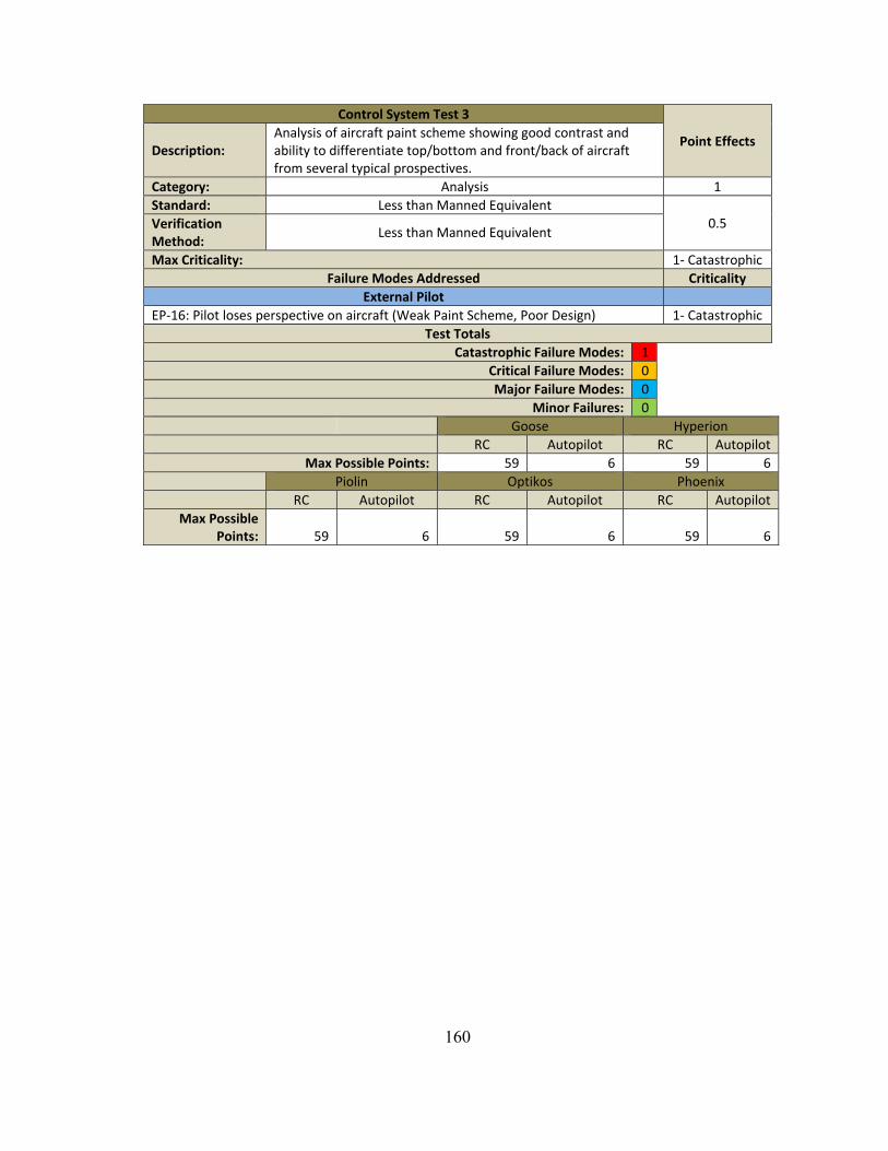
160

Control System Test 3

Point Effects Description: 

Analysis of aircraft paint scheme showing good contrast and ability to differentiate top/bottom and front/back of aircraft from several typical prospectives. 

Category:  Analysis 1Standard:  Less than Manned Equivalent

0.5 Verification Method: 

Less than Manned Equivalent 

Max Criticality:  1‐ CatastrophicFailure Modes Addressed Criticality

External PilotEP‐16: Pilot loses perspective on aircraft (Weak Paint Scheme, Poor Design) 1‐ Catastrophic

Test TotalsCatastrophic Failure Modes:  1 

Critical Failure Modes:  0 Major Failure Modes:  0 

Minor Failures:  0    Goose  Hyperion

   RC Autopilot RC  AutopilotMax Possible Points: 59 6 59  6

  Piolin Optikos Phoenix  RC  Autopilot RC Autopilot RC  Autopilot

Max Possible Points:  59  6  59  6  59  6 

161

Control System Test 4 

Point Effects Description: 

Initial Flight Test (Aircraft is put through its paces, but not pushed to the edge of the envelope) 

Category:  Flight Test 3Standard:  Less than Manned Equivalent

0.5 Verification Method: 

Less than Manned Equivalent 

Max Criticality:  1‐ CatastrophicFailure Modes Addressed Criticality

External Pilot  EP‐1: Aircraft handling characters too poor for pilot to compensate (Poor Design)  1‐ CatastrophicEP‐2: RC Hardware Failure (Poor Design) 1‐ CatastrophicEP‐4: RC Hardware Failure (Manf. Defect) 1‐ CatastrophicEP‐5: RC Hardware Failure (Batteries defective) 1‐ CatastrophicEP‐6: RC Software Failure (Functional Requirement Failure) 1‐ CatastrophicEP‐7: A/C flies beyond TX Range (Poor Design) 1‐ CatastrophicEP‐8: A/C flies beyond TX Range (Manf. Defect) 1‐ CatastrophicEP‐9: A/C flies beyond TX range (Improper Operations) 1‐ CatastrophicEP‐10: EMI causes momentary drop of control link (Poor Design) 3 ‐ MajorEP‐11: EMI causes momentary drop of control link (Manf. Defect) 3 ‐ MajorEP‐12: EMI causes momentary drop of control link (Environmental Factors) 3 ‐ MajorEP‐13: EMI causes extended drop of control link (Poor Design) 1‐ CatastrophicEP‐14: EMI causes extended drop of control link (Manf. Defect) 1‐ CatastrophicEP‐15: EMI causes extended drop of control link (Environmental Factors) 1‐ CatastrophicEP‐16: Pilot loses perspective on aircraft (Weak Paint Scheme) 2 ‐ CriticalEP‐17: Pilot loses perspective on aircraft (Flown too far away, improper procedures)  2 ‐ Critical

Test TotalsCatastrophic Failure Modes: 10 

Critical Failure Modes: 2 Major Failure Modes: 3 

Minor Failures: 0    Goose  Hyperion

   RC Autopilot RC  AutopilotMax Possible Points: 2286 202 2286  202

  Piolin  RC  Autopilot RC Autopilot RC  Autopilot

Max Possible Points:  2286  202  2286  202  2286  202 

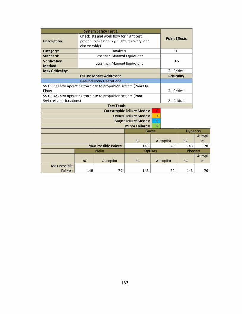
162

System Safety Test 1

Point Effects Description: 

Checklists and work flow for flight test procedures (assembly, flight, recovery, and disassembly) 

Category:  Analysis 1 Standard:  Less than Manned Equivalent

0.5 Verification Method: 

Less than Manned Equivalent 

Max Criticality:  2 ‐ Critical Failure Modes Addressed Criticality Ground Crew Operations   

SS‐GC‐1: Crew operating too close to propulsion system (Poor Op. Flow)  2 ‐ Critical SS‐GC‐4: Crew operating too close to propulsion system (Poor Switch/hatch locations)  2 ‐ Critical 

Test TotalsCatastrophic Failure Modes: 0

Critical Failure Modes: 2Major Failure Modes: 0

Minor Failures: 0   Goose  Hyperion

   RC  Autopilot  RC Autopilot 

Max Possible Points: 148 70  148  70  Piolin Optikos Phoenix 

RC  Autopilot  RC  Autopilot  RC Autopilot 

Max Possible Points:  148  70  148  70  148  70 

163

System Safety Test 2Point Effects 

Description: Supervised dry run through checklists and workflows with aircraft components. 

Category:  Physical Ground Test 2 Standard:  Less than Manned Equivalent

0.5 Verification Method: 

Less than Manned Equivalent 

Max Criticality:  1‐ CatastrophicFailure Modes Addressed Criticality Ground Crew Operations   

SS‐GC‐1: Working too close to propulsion system (Poor Design) 2 ‐ Critical SS‐GC‐2: Working too close to prop. system(Activation outside of operation flow)   2 ‐ Critical SS‐GC‐3: Working too close to prop. System (GC not following standard operational flow)  2 ‐ Critical SS‐GC‐4: Crew operating too close to propulsion system (Poor Switch/hatch locations)  2 ‐ Critical SS‐GC‐5: GC supplies are hazardous (Unavoidable) 1‐ CatastrophicSS‐GC‐6: GC supplies are hazardous (Avoidable) 1‐ CatastrophicSS‐GC‐7: Crew unaware that prop. System is active  2 ‐ Critical SS‐GC‐8: Prop. System activates outside of normal operational flow 2 ‐ Critical SS‐GC‐9: Crew not following standard op flow results in prop. System activation. 2 ‐ Critical 

Test TotalsCatastrophic Failure Modes: 2

Critical Failure Modes: 7Major Failure Modes: 0

Minor Failures: 0   Goose  Hyperion

   RC  Autopilot  RC Autopil

ot Max Possible Points: 1406 666  1406  666

  Piolin Optikos Phoenix 

RC  Autopilot  RC  Autopilot  RC Autopil

ot Max Possible Points:  1406  666 1406 666  1406  666

164

System Safety Test 3Point Effects 

Description: Initial Flight Tests.  Documenting how the ground crew operations performed. 

Category:  Flight Test 3 Standard:  Less than Manned Equivalent

0.5 Verification Method: 

Less than Manned Equivalent 

Max Criticality:  1‐ CatastrophicFailure Modes Addressed Criticality Ground Crew Operations   

SS‐GC‐1: Working too close to propulsion system (Poor Design) 2 ‐ Critical SS‐GC‐2: Working too close to prop. system(Activation outside of operation flow)   2 ‐ Critical SS‐GC‐3: Working too close to prop. System (GC not following standard operational flow)  2 ‐ Critical SS‐GC‐4: Crew operating too close to propulsion system (Poor Switch/hatch locations)  2 ‐ Critical SS‐GC‐5: GC supplies are hazardous (Unavoidable) 1‐ CatastrophicSS‐GC‐6: GC supplies are hazardous (Avoidable) 1‐ CatastrophicSS‐GC‐7: Crew unaware that prop. System is active  2 ‐ Critical SS‐GC‐8: Prop. System activates outside of normal operational flow 2 ‐ Critical SS‐GC‐9: Crew not following standard op flow results in prop. System activation.  2 ‐ Critical 

Test TotalsCatastrophic Failure Modes: 2

Critical Failure Modes: 7Major Failure Modes: 0

Minor Failures: 0   Goose  Hyperion

   RC  Autopilot  RC 

Autopilot 

Max Possible Points:  2109  999  2109 999 

  Piolin Optikos Phoenix 

RC  Autopilot  RC  Autopilot  RC 

Autopilot 

Max Possible Points:  2109  999  2109  999  2109 

999 

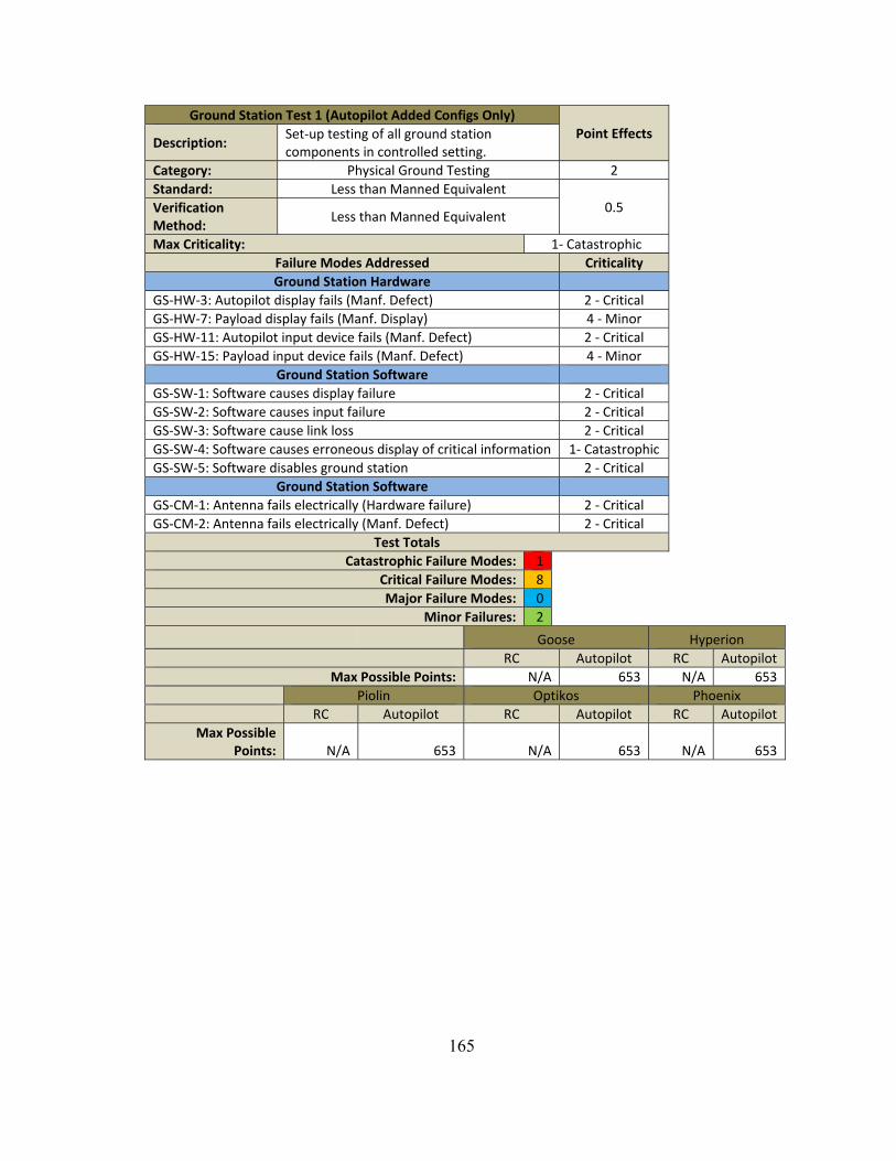
165

Ground Station Test 1 (Autopilot Added Configs Only)Point Effects 

Description: Set‐up testing of all ground station components in controlled setting. 

Category:  Physical Ground Testing 2Standard:  Less than Manned Equivalent

0.5 Verification Method: 

Less than Manned Equivalent 

Max Criticality:  1‐ Catastrophic Failure Modes Addressed Criticality Ground Station Hardware

GS‐HW‐3: Autopilot display fails (Manf. Defect) 2 ‐ Critical GS‐HW‐7: Payload display fails (Manf. Display) 4 ‐Minor GS‐HW‐11: Autopilot input device fails (Manf. Defect) 2 ‐ Critical GS‐HW‐15: Payload input device fails (Manf. Defect) 4 ‐Minor 

Ground Station SoftwareGS‐SW‐1: Software causes display failure 2 ‐ Critical GS‐SW‐2: Software causes input failure 2 ‐ Critical GS‐SW‐3: Software cause link loss  2 ‐ Critical GS‐SW‐4: Software causes erroneous display of critical information 1‐ Catastrophic GS‐SW‐5: Software disables ground station 2 ‐ Critical 

Ground Station SoftwareGS‐CM‐1: Antenna fails electrically (Hardware failure) 2 ‐ Critical GS‐CM‐2: Antenna fails electrically (Manf. Defect) 2 ‐ Critical 

Test TotalsCatastrophic Failure Modes: 1

Critical Failure Modes: 8Major Failure Modes: 0

Minor Failures: 2

      Goose   Hyperion    RC Autopilot  RC  Autopilot

Max Possible Points: N/A 653  N/A  653  Piolin Optikos Phoenix  RC  Autopilot RC Autopilot  RC  Autopilot

Max Possible Points:  N/A  653  N/A  653  N/A  653 

166

Appendix C

Example Showing Units Error in Casualty Expectation Equation from RCC-323-99

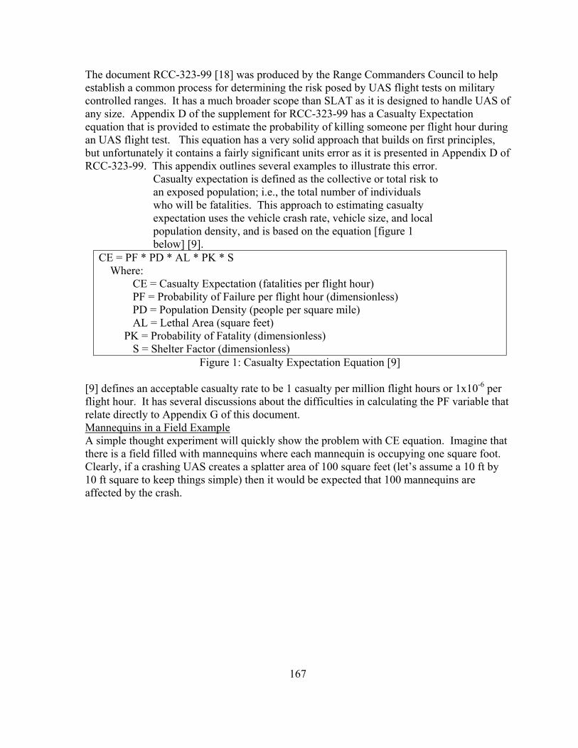
167

The document RCC-323-99 [18] was produced by the Range Commanders Council to help establish a common process for determining the risk posed by UAS flight tests on military controlled ranges. It has a much broader scope than SLAT as it is designed to handle UAS of any size. Appendix D of the supplement for RCC-323-99 has a Casualty Expectation equation that is provided to estimate the probability of killing someone per flight hour during an UAS flight test. This equation has a very solid approach that builds on first principles, but unfortunately it contains a fairly significant units error as it is presented in Appendix D of RCC-323-99. This appendix outlines several examples to illustrate this error.

Casualty expectation is defined as the collective or total risk to an exposed population; i.e., the total number of individuals who will be fatalities. This approach to estimating casualty expectation uses the vehicle crash rate, vehicle size, and local population density, and is based on the equation [figure 1 below] [9].

CE = PF * PD * AL * PK * S Where: CE = Casualty Expectation (fatalities per flight hour) PF = Probability of Failure per flight hour (dimensionless) PD = Population Density (people per square mile) AL = Lethal Area (square feet) PK = Probability of Fatality (dimensionless) S = Shelter Factor (dimensionless)

Figure 1: Casualty Expectation Equation [9] [9] defines an acceptable casualty rate to be 1 casualty per million flight hours or 1x10-6 per flight hour. It has several discussions about the difficulties in calculating the PF variable that relate directly to Appendix G of this document. Mannequins in a Field Example A simple thought experiment will quickly show the problem with CE equation. Imagine that there is a field filled with mannequins where each mannequin is occupying one square foot. Clearly, if a crashing UAS creates a splatter area of 100 square feet (let’s assume a 10 ft by 10 ft square to keep things simple) then it would be expected that 100 mannequins are affected by the crash.

168

Step 1: Defining Variables

Table 1: Variable Definitions for Mannequin Example

CE = 100 Based on this example it is expected that 100 mannequins would be casualties of the UAS crash.

PF = 1 In this example the aircraft is assumed to be crashing so the probability of failure is one.

PD = 27,878,400

Since the mannequins are each occupying one square foot of the field the population density per square mile would be 27,878,400 (the number of square feet in a square mile).

AL = 100 Based on the conditions of the example the lethal area of the UAS crash site is 100 square feet.

PK = 1 For this example we will assume any mannequin struck by the crashing UAS is a fatality.

S = 1 To make this simple the Shelter Factor (S) is considered to be 1 (No Shelter). This is stated by the example description as being out in a field where there is no shelter.

Step 2: Substituting Values CE = PF * PD * AL * PK * S CE = (1)(27,878,400)(100) (1)(1) CE = (27,878,400)(100) CE = 2,787,840,000 dead mannequins ≠ 100 mannequins expected Step 3: Analysis of Problem Clearly it is unlikely that 2.7 billion mannequins would be killed in a 100 square foot crash area. The problem lies in the units difference between PD and AL. The population density (PD) is in people per square mile while the lethal area (AL) is in square feet. This equation is multiplying point estimates together, which can only be done if the units are the same. The way the equation is defined the lethal area is effectively being treated like it is in units of square miles rather than square feet. A quick analysis of the results shows that if 2,787,840,000 is divided by the number of square feet in a mile (27,878,400) then the expected CE result of 100 “dead” mannequins is found. The equation as defined in [9] is off by a factor of approximately 28 million. This error makes the CE equation significantly overly conservative, which although better than being under conservative by 28 million reduces its usefulness. The correct equation should divide the AL value by 27,878,400 in order to convert the lethal area into square miles as shown in equation the below.

27,878,400

169

Appendix D

Mapping from MIL-HDBK-516 to SLAT

170

Appendix D Format and Key Terms This appendix shows the mapping of each of the sections from MIL-HDBK-516 into SLAT. This mapping is performed as a method of showing the paradigm changes between manned and unmanned aircraft. Each chapter in MIL-HDBK-516 is addressed separately so that discussion about each chapter can be done along the way. There are several key terms that are used in reference to the mapping, which are shown below to help make this appendix easier to follow.

Direct Mapping (Domain-FMECA) This shows that there is a clear mapping from MIL-HDBK-516 into one of the SLAT domains. If applicable the specific FMECA will be noted.

No Mapping (UAS Context)

This indicates that no mapping exists because the MIL-HDBK-516B section is specific to manned aviation. This is typical of items such as ejection seats, crew comfort, or internal aircraft lighting. There will typically be a short note explaining why these items are considered specific to manned aviation.

No Mapping (Scope)32

This indicates that no mapping exists because it is beyond the scope of SLAT. This is often the case for many of the airworthiness process items in MIL-HDBK-516B and for airworthiness criteria relevant to rotary wing aircraft as SLAT is designed for fixed wing only. There will typically be a short note explaining why these items are considered outside of the scope of SLAT.

Distributed Mapping

This indicates that many of the criteria in the noted section of MIL-HDBK-516 are addressed in SLAT, but that they are spread out across numerous domains. There is no one to one mapping that can be made, but the criteria are applicable. There will be a discussion on each item marked as having a “Distributed Mapping”.

Obscure Mapping(Domain)

This indicates that the criteria in the noted section of MIL-HDBK-516 don’t map well into SLAT. Often this denotes that there are some concepts that have parallels in the approach taken by SLAT, but that it isn’t necessarily a true mapping from each criterion for manned aircraft to SLAT items. If applicable the domain with the most parallels will be noted in parenthesis. There will be a discussion on each item marked as having an “Obscure Mapping”.

32 The scope for SLAT is defined as fixed wing UAS between 350 and 2 lb.  Airspace integration aspects such as See and Avoid are beyond the scope of SLAT at the moment. 

171

MIL-HDBK-516 SLAT

Chapter 4 – Systems Engineering 4.1 – Design Criteria Obscure Mapping 4.2 – Tools & Databases Obscure Mapping 4.3 – Materials Selection Distributed Mapping 4.4 – Manf. & Quality Distributed Mapping 4.5 – Manuals Distributed Mapping 4.6 – Config. Identification Direct Mapping (System Safety) 4.7 – Config. Status Direct Mapping (System Safety)

Many of the Systems Engineering criteria in MIL-HDBK-516 don’t map directly into SLAT because they are primarily the process directives to insure that the airworthiness process is properly established. Ensuring the Design Criteria (section 4.1) is mostly outside of the scope of SLAT although the failure modes that could be exposed due to inadequate design scope could occur. Primarily SLAT is designed as a tool to help ensure the design criteria are properly defined and met. Likewise, SLAT could be viewed as one of the tools to use in the certification process. SLAT leaves the determination of acceptable verification methods up to the graders of each of the test, while building in the flexibility of not forcing a set of acceptable tools. The failure modes associated with Materials Selection (4.3) are captured in the individual component failure modes and are therefore distributed across every domain except System Safety. Manufacturing defects are one of the most common causal factors across all of the domains so the criteria in Section 4.4 are also distributed across every domain except System Safety. Section 4.5 (Manuals) is primarily a maintenance item. Since maintenance failure modes are embedded in each of the domains there will be parts of SLAT in every domain that grant points for proper manuals and technical documents to the equipment associated with that domain. Configuration control (4.6-7) is primarily captured in System Safety.

172

MIL-HDBK-516 SLAT Chapter 5 – Structures

5.1 – Loads Direct Mapping(Structures) 5.2 – Structural Dynamics Direct Mapping(Structures) 5.3 – Strength Direct Mapping(Structures) 5.4 – Fatigue Direct Mapping(Structures) 5.5 – Mass Properties Distributed Mapping 5.6 – Flight Release No Mapping(Scope)

Chapter 5 maps relatively cleaning into the Structures domain in SLAT. The exceptions are Section 5.5 and Section 5.6. The Mass Properties criteria are mainly related to weight and balance items. In SLAT these requirements are distributed between Fuel Systems (e.g. center of gravity change due to fuel use), maintenance items inside the Structures domain (e.g. ensuring the vehicle is properly balanced), System Safety (ensuring that the proper checklists for vehicle balancing are available), and Control Systems (e.g. ensuring that the autopilot can safely fly the aircraft in its current configuration). The Flight Release criterion is outside of the scope of SLAT. SLAT is a tool to help in the Flight Release process, but it leaves the actual process elements to the appropriate certifying authority.

173

MIL-HDBK-516 SLAT Chapter 6 – Flight Technology

6.1 – Stability and Controls Direct Mapping(Control Systems)

Direct Mapping(Ground Station) Direct Mapping(System Safety)

6.2 – Vehicle Control Functions

Direct Mapping(Control Systems) Direct Mapping(Structures – Control

Surfaces) Direct Mapping(Electrical -

Direct Mapping(Ground Station) 6.3 – Aerodynamics and Performance

Direct Mapping(Control Systems) Direct Mapping(Propulsion)

Chapter 6 of MIL-HDBK-516 mostly maps into the Control Systems domain of SLAT. This is expected since without a pilot on-board the desire is to ensure that closed-loop handling characteristics are appropriate (i.e. as long as the autopilot can control the aircraft the open-loop handling characteristics or stability don’t matter). In many cases the term pilot can be replaced with autopilot. In Section 6.1 the warning functions for wrong configuration would map into the Ground Station domain (where the warning message is actually displayed to the operator) and to the System Safety – Autopilot Operator to Vehicle Interface (for the human factors aspects of actually communicating the message to the operator). Some of the Vehicle Control Functions map into the “Structures – Control Surface” and “Electrical – Servos” FMECA sets for items such as ensuring that hinge moments are acceptable and that the actuator limitations are taken into accounts. There are some criteria in Section 6.3 that will map more appropriately into the Propulsion domain as the resulting failure modes are typically loss of propulsion.

174

MIL-HDBK-516 SLAT Chapter 7 – Propulsion

7.1 – Propulsion Safety Management

Obscure Mapping(System Safety) Distributed Mapping

7.2 – Gas Turbine Engine Applications

Direct Mapping(Propulsion – Jet Engines)

7.3 – Alternate Propulsion Systems

Direct Mapping(Propulsion – Electric Motor) Direct Mapping(Propulsion – Reciprocating

Engine) Most of the criteria in Chapter 7 map very clearly to the Propulsion domain in SLAT, but one notable exception is the Propulsion Safety Management requirements. Many of these criteria are captured by “System Safety – Ground Operations” where there is significant analysis of hazard to crew members from the propulsion system. In SLAT a Propulsion Safety Management plan would likely be what is delivered to address those hazards, but it isn’t directly mandated by SLAT. Some other aspects of a Propulsion Safety Management plan could be distributed through other domains as they address failure modes such as fuel corroding wiring.

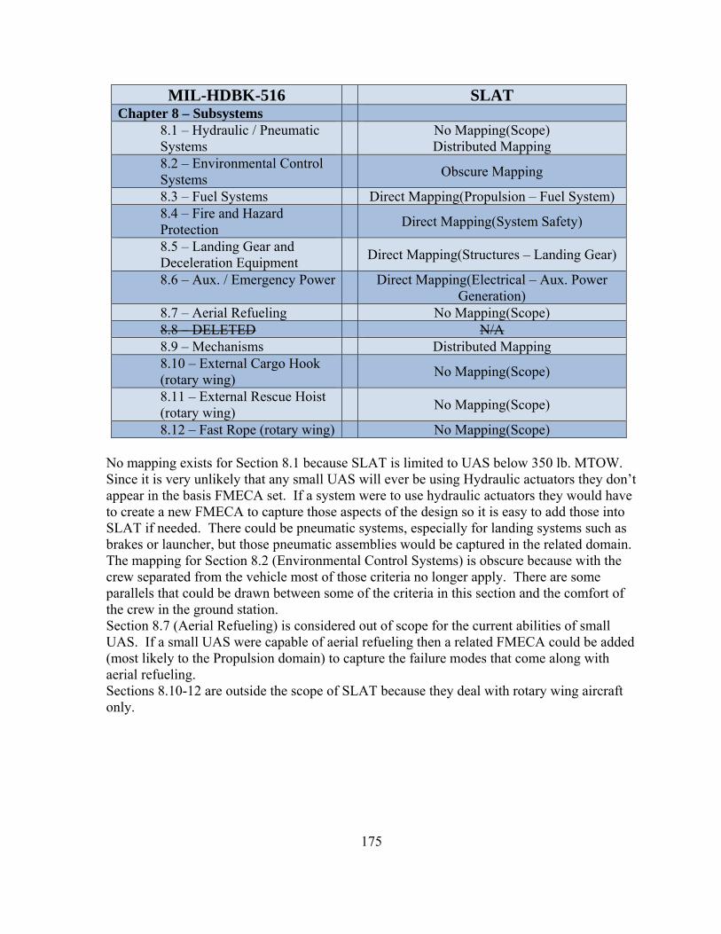
175

MIL-HDBK-516 SLAT Chapter 8 – Subsystems

8.1 – Hydraulic / Pneumatic Systems

No Mapping(Scope) Distributed Mapping

8.2 – Environmental Control Systems

Obscure Mapping

8.3 – Fuel Systems Direct Mapping(Propulsion – Fuel System) 8.4 – Fire and Hazard Protection

Direct Mapping(System Safety)

8.5 – Landing Gear and Deceleration Equipment

Direct Mapping(Structures – Landing Gear)

8.6 – Aux. / Emergency Power Direct Mapping(Electrical – Aux. Power Generation)

8.7 – Aerial Refueling No Mapping(Scope) 8.8 – DELETED N/A 8.9 – Mechanisms Distributed Mapping 8.10 – External Cargo Hook (rotary wing)

No Mapping(Scope)

8.11 – External Rescue Hoist (rotary wing)

No Mapping(Scope)

8.12 – Fast Rope (rotary wing) No Mapping(Scope) No mapping exists for Section 8.1 because SLAT is limited to UAS below 350 lb. MTOW. Since it is very unlikely that any small UAS will ever be using Hydraulic actuators they don’t appear in the basis FMECA set. If a system were to use hydraulic actuators they would have to create a new FMECA to capture those aspects of the design so it is easy to add those into SLAT if needed. There could be pneumatic systems, especially for landing systems such as brakes or launcher, but those pneumatic assemblies would be captured in the related domain. The mapping for Section 8.2 (Environmental Control Systems) is obscure because with the crew separated from the vehicle most of those criteria no longer apply. There are some parallels that could be drawn between some of the criteria in this section and the comfort of the crew in the ground station. Section 8.7 (Aerial Refueling) is considered out of scope for the current abilities of small UAS. If a small UAS were capable of aerial refueling then a related FMECA could be added (most likely to the Propulsion domain) to capture the failure modes that come along with aerial refueling. Sections 8.10-12 are outside the scope of SLAT because they deal with rotary wing aircraft only.

176

MIL-HDBK-516 SLAT Chapter 9 – Crew Systems

9.1 – Escape / Egress System No Mapping(UAS Context) 9.2 – Crew Stations / Aircraft Interiors

No Mapping(UAS Context)

9.3 – Air Vehicle Lighting No Mapping(UAS Context)

9.4 – Human Performance Direct Mapping(Ground Station – Human Performance)

9.5 – Life Support Systems No Mapping(UAS Context) 9.6 – Transparency Integration

No Mapping(UAS Context)

9.7 – Crash Survivability No Mapping(UAS Context) 9.8 – Air Transportability and Airdrop

No Mapping(UAS Context)

9.9 – Lavatories, Galleys, and Areas Not Continuously Occupied

No Mapping(UAS Context)

The vast majority of Chapter 9 doesn’t map into SLAT at all because it is all focused on the safety and comfort of the on-board crew members. The Human Performance part though does map directly into the ground station. These criteria are focused on the communication of information to the crew and the crew’s interface to the vehicle. The vast majority of these criteria are still very relevant to remote operation.

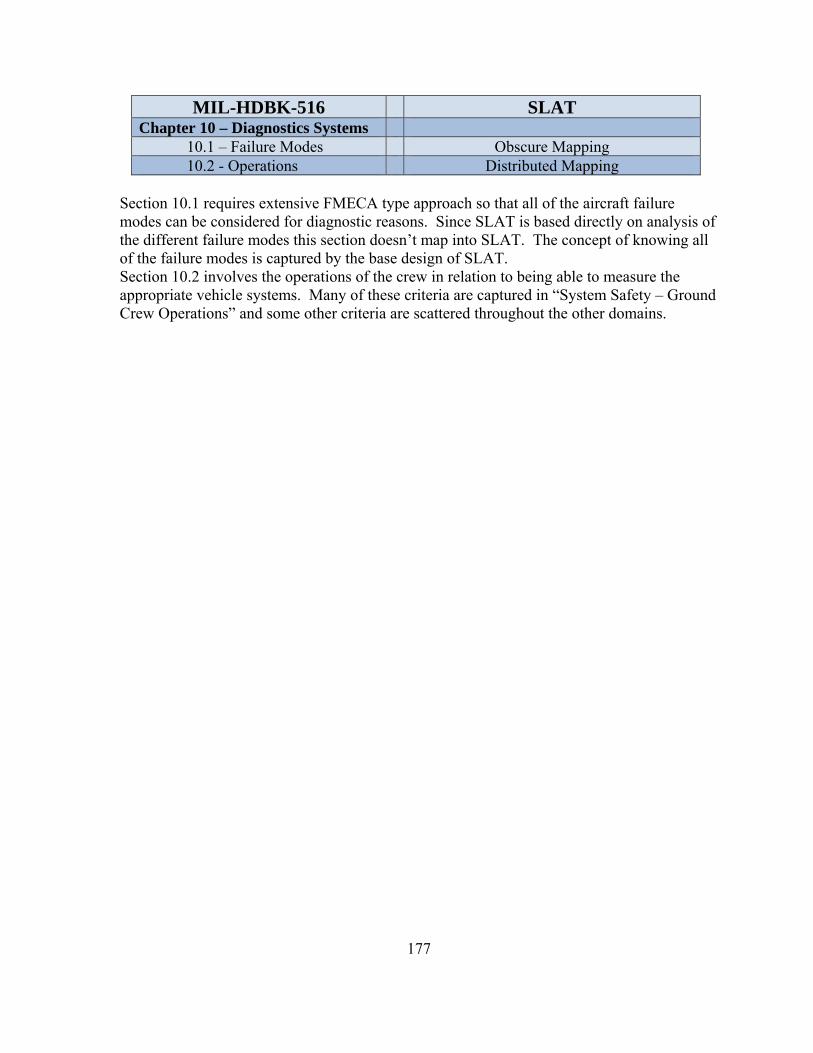
177

MIL-HDBK-516 SLAT Chapter 10 – Diagnostics Systems

10.1 – Failure Modes Obscure Mapping 10.2 - Operations Distributed Mapping

Section 10.1 requires extensive FMECA type approach so that all of the aircraft failure modes can be considered for diagnostic reasons. Since SLAT is based directly on analysis of the different failure modes this section doesn’t map into SLAT. The concept of knowing all of the failure modes is captured by the base design of SLAT. Section 10.2 involves the operations of the crew in relation to being able to measure the appropriate vehicle systems. Many of these criteria are captured in “System Safety – Ground Crew Operations” and some other criteria are scattered throughout the other domains.

178

MIL-HDBK-516 SLAT Chapter 11 – Avionics

11.1 – Avionics Architecture Direct Mapping(Control Systems) Direct Mapping(Ground Station)

11.2 – Avionics Subsystems Direct Mapping(Control Systems) Direct Mapping(Ground Station)

11.3 – Avionics Air Vehicle Installation

Distributed Mapping

The criteria in 11.1 and 11.2 clearly map to the electronics items in and that the proper checklists are available the Control Systems domain and the Ground Station domains. The mapping of the installation issues from 11.3 though map into several different areas. Criterion 11.3.1 deals with ensuring that the equipment installation is adequate for SOF. This item is captured by many of the failure modes in the FMECA, but no single failure mode maps directly to this SOF criterion. Criterion 11.3.2 deals with flight and maintenance manuals so that aspect would be captured by the maintenance items within the Control Systems or Electrical domain. Criterion 11.3.3 handles antenna coverage issues. The integrity of the data link is a primary concern for remotely operated systems and as such has its own FMECA in the Ground Station domain, which captures this criterion in significant detail.

179

MIL-HDBK-516 SLAT Chapter 12 – Electrical

12.1 – Electrical Power Generation System

Direct Mapping(Electrical – Power Generation)

12.2 – Electrical Wiring / Power Distribution

Direct Mapping(Electrical – Wiring/Connectors)

Chapter 12 maps very cleanly into the Electrical domain in SLAT.

180

MIL-HDBK-516 SLAT Chapter 13 – E3

13.1 – Component / Subsystem E3 Qualification

Obscure Mapping(System Safety)

13.2 – System Level E3 Qualification

Obscure Mapping(System Safety)

Chapter 13, which deals with Electromagnetic Environmental Effects (E3), does not have a distinct mapping into SLAT. There are several failure modes distributed throughout the SLAT basis FMECA sets (primarily in Electrical and Ground Station domains) that address Electromagnetic Interference and other failure modes commonly associated with E3, but there is no one domain that captures these criteria directly. The System Safety domain captures the majority of the intent of the criteria in Chapter 13 by handling the high level SOF issues that can arise with E3 type failures.

181

MIL-HDBK-516 SLAT Chapter 14 – System Safety

14.1 – System Safety Program

Obscure Mapping(System Safety)

14.2 – Safety Design Requirements

Obscure Mapping(System Safety)

14.3 – Software Safety Program

Obscure Mapping

Even though there is a System Safety domain in SLAT the individual criterion discussed in Chapter 14 of MIL-HDBK-516B don’t map directly into that domain. This is due to the procedural nature of Chapter 14 versus the failure mitigation nature of SLAT. Many of the criteria in Chapter 14 are directed at establishing a safety program to ensure that the important failure modes are known and addressed. SLAT is based on this process so the tailoring of the FMECA captures many of the aspects instituted through the use of a safety program. A safety program would likely be one of the primary artifacts presented to get points for the System Safety domain, but it would be focused on risk mitigation rather than fulfilling a requirement for a safety plan. Likewise, many of the safety design requirements in section 14.2 are incorporated in the foundation of SLAT and therefore those criteria don’t have a direct mapping into the items of SLAT.

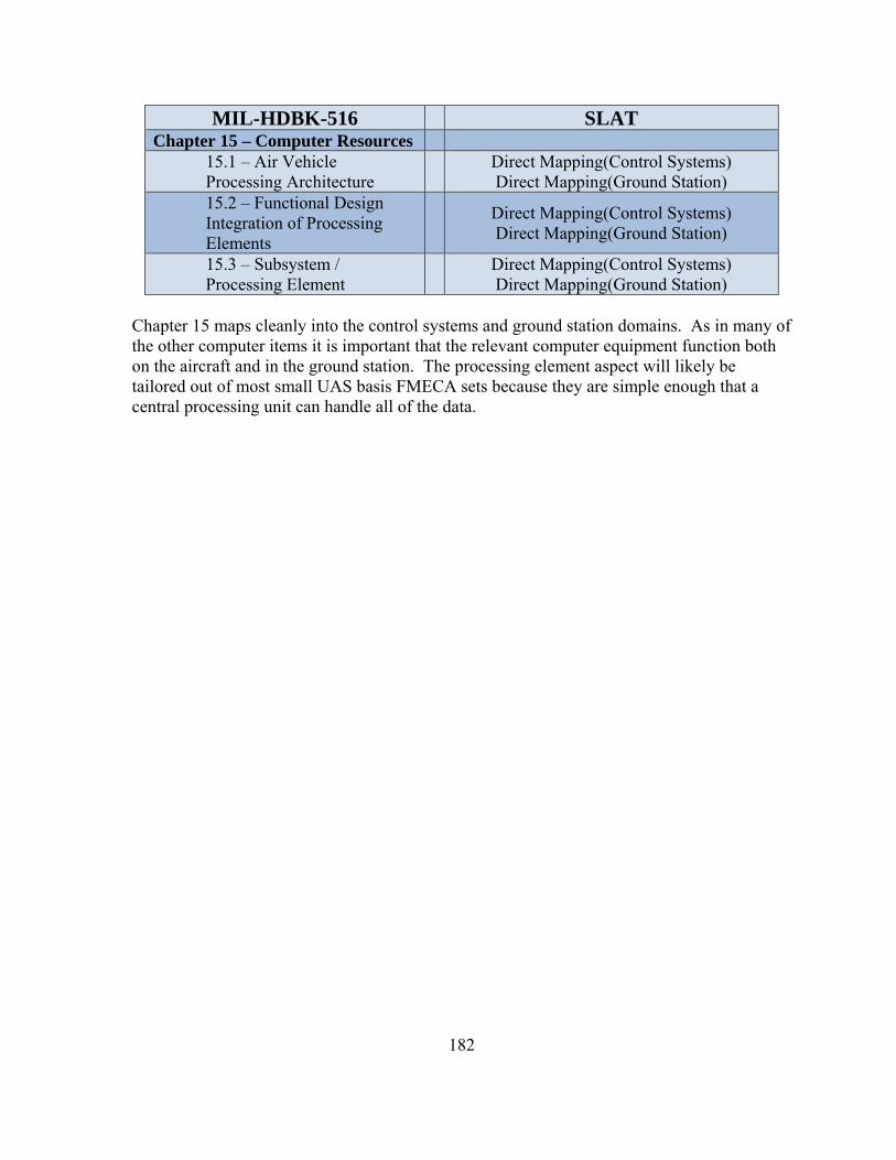
182

MIL-HDBK-516 SLAT Chapter 15 – Computer Resources

15.1 – Air Vehicle Processing Architecture

Direct Mapping(Control Systems) Direct Mapping(Ground Station)

15.2 – Functional Design Integration of Processing Elements

Direct Mapping(Control Systems) Direct Mapping(Ground Station)

15.3 – Subsystem / Processing Element

Direct Mapping(Control Systems) Direct Mapping(Ground Station)

Chapter 15 maps cleanly into the control systems and ground station domains. As in many of the other computer items it is important that the relevant computer equipment function both on the aircraft and in the ground station. The processing element aspect will likely be tailored out of most small UAS basis FMECA sets because they are simple enough that a central processing unit can handle all of the data.

183

MIL-HDBK-516 SLAT Chapter 16 – Maintenance

16.1 – Maintenance Manuals and Checklists

Distributed Mapping

16.2 – Inspection Requirements

Distributed Mapping

There is no specific maintenance domain of SLAT due to the point allocation process being tied to the number of failure modes in each domain. As a result the maintenance items are distributed across all of the domains with physical components (e.g. System Safety has no maintenance items).

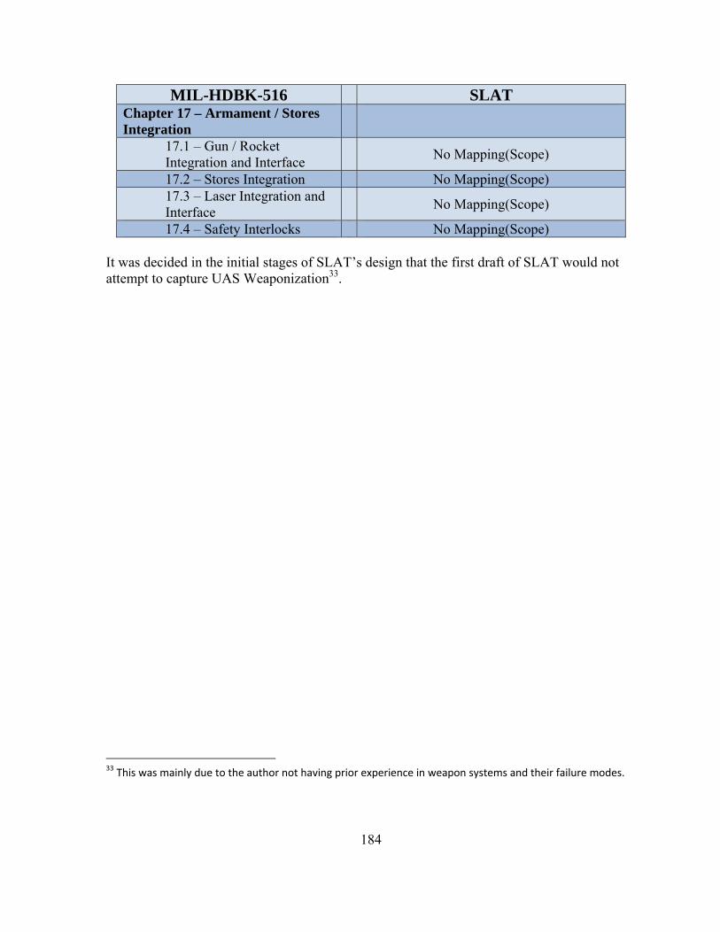
184

MIL-HDBK-516 SLAT Chapter 17 – Armament / Stores Integration

17.1 – Gun / Rocket Integration and Interface

No Mapping(Scope)

17.2 – Stores Integration No Mapping(Scope) 17.3 – Laser Integration and Interface

No Mapping(Scope)

17.4 – Safety Interlocks No Mapping(Scope) It was decided in the initial stages of SLAT’s design that the first draft of SLAT would not attempt to capture UAS Weaponization33.

33 This was mainly due to the author not having prior experience in weapon systems and their failure modes. 

185

MIL-HDBK-516 SLAT Chapter 18 – Passenger Safety

18.1 – Survivability of Passengers

No Mapping(UAS Context)

18.2 – Fire Resistance No Mapping(UAS Context) 18.3 – Physiology Requirements of Passengers

No Mapping(UAS Context)

The entire chapter on Passenger Safety is not a concern on unmanned systems.

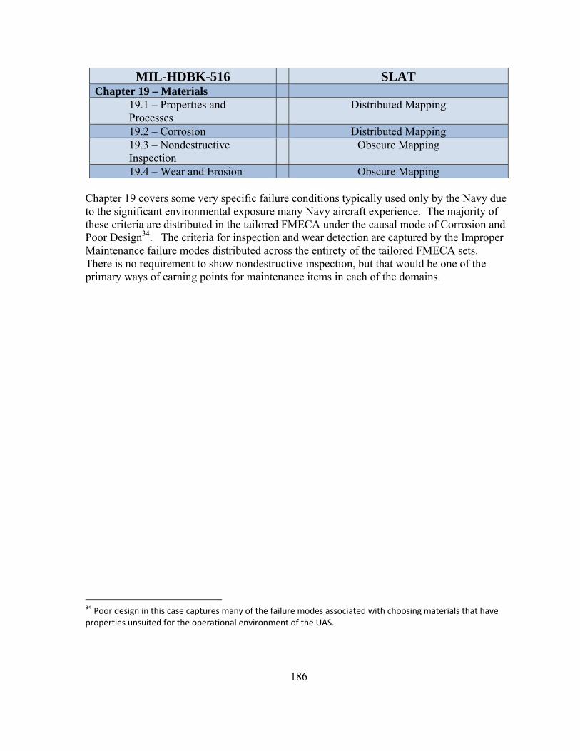
186

MIL-HDBK-516 SLAT Chapter 19 – Materials

19.1 – Properties and Processes

Distributed Mapping

19.2 – Corrosion Distributed Mapping 19.3 – Nondestructive Inspection

Obscure Mapping

19.4 – Wear and Erosion Obscure Mapping Chapter 19 covers some very specific failure conditions typically used only by the Navy due to the significant environmental exposure many Navy aircraft experience. The majority of these criteria are distributed in the tailored FMECA under the causal mode of Corrosion and Poor Design34. The criteria for inspection and wear detection are captured by the Improper Maintenance failure modes distributed across the entirety of the tailored FMECA sets. There is no requirement to show nondestructive inspection, but that would be one of the primary ways of earning points for maintenance items in each of the domains.

34 Poor design in this case captures many of the failure modes associated with choosing materials that have properties unsuited for the operational environment of the UAS. 

187

MIL-HDBK-516 SLAT Chapter 20 – Other

20.1 – Mission/Test Equipment and Cargo/Payload Safety

No Mapping(Scope)

The criteria in Chapter 20 are beyond the scope of SLAT’s initial design.

188

Appendix E

Operational Flight Tests

In the UAS industry much emphasis is placed on successful operational flight hours, but SLAT does not give any points for operational flight hours due to the diffused and inconsistent state of such data35. This appendix outlines the statistics behind calculating the 95% confidence bounds on UAS reliability given several different examples of how operational flight hours might be presented to a CA. This shows that the number of hours needed to truly show that an UAS has reached a significantly safe reliability is exceedingly high. The equations in this appendix are cited from Chapter 10: Reliability Engineering in Probability and Its Applications for Engineers [28]. All of the examples in the appendix are modifications of examples from [28].

35 Typically operational flight‐hours data is presented with no information about the conditions of the flight day or the exact configuration of the aircraft.  With UAS there are further issues when regarding operational flight hours, especially in the military context, when the operators may have decided to take significant risks with the aircraft because it is unmanned (e.g. During a military operation an UAS providing critical surveillance of the mission suffers a failure that would typically result in immediately returning the aircraft to its base of operations.  The commander decides that the risk to the soldiers on the ground if the UAS is not assisting is significantly higher than the risk of losing the UAS so the aircraft stays on station despite the failure.  This could easily result in the loss of the UAS even though the diagnostics system worked properly and the aircraft could have returned to base). 

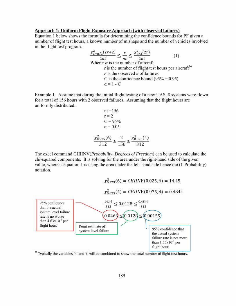
189

Approach 1: Uniform Flight Exposure Approach (with observed failures) Equation 1 below shows the formula for determining the confidence bounds for PF given a number of flight test hours, a known number of mishaps and the number of vehicles involved in the flight test program.

⁄ ⁄ (1) Where: n is the number of aircraft t is the number of flight test hours per aircraft36 r is the observed # of failures C is the confidence bound (95% = 0.95) α = 1 - C Example 1. Assume that during the initial flight testing of a new UAS, 8 systems were flown for a total of 156 hours with 2 observed failures. Assuming that the flight hours are uniformly distributed: nt =156 r = 2 C = 95% α = 0.05

. 6312

2156

. 4312

The excel command CHIINV(Probability, Degrees of Freedom) can be used to calculate the chi-squared components. It is solving for the area under the right-hand side of the given value, whereas equation 1 is using the area under the left-hand side hence the (1-Probability) notation. . 6 0.025, 6 14.45 . 4 0.975, 4 0.4844 . 0.0128 . 0.0463 0.0128 0.00155 36 Typically the variables ‘n’ and ‘t’ will be combined to show the total number of flight test hours. 

95% confidence that the actual system failure rate is not more than 1.55x10-3 per flight hour.

Point estimate of system level failure

95% confidence that the actual system level failure rate is no worse than 4.63x10-2 per flight hour.

190

This shows that the point estimation of the failure rate is still 1.28x10-2 as previously proposed, but that the lower 95% confidence bound is only 4.63x10-2. The upper confidence bound says that it is very unlikely given the flight test data that the actual PF is any higher than 1.55x10-3. Note: This approach is modeling the flight testing as a time truncation experiment where as items fail they are replaced until a certain amount of time is reached (in this case the current amount of flight test hours). This approach works well when limited flight test data is available. The Discrete Flight Exposure approach will give a more accurate confidence bound assuming the additional information is available.

191

Approach 2: Discrete Flight Exposure Approach (with observed failures) This approach only works if there is detailed information about the flight test series for an aircraft. Equation 2 below shows the formula for determining the confidence bounds for PF given a number of flight test hours and vehicles.

⁄ ⁄ (2) Where: τ is the weighted exposure hours r is the observed # of failures C is the confidence bound (95% = 0.95) α = 1 - C Example 2. Assume that during the initial flight testing of a new UAS, 8 systems were flown with the following results: UAS1 flew 81 hrs before crashing UAS2 flew 120 hrs before crashing UAS3 flew 220 hrs before crashing UAS4 flew 51 hrs before crashing UAS5-UAS8 flew 235 hrs each without incident 81 120 220 51 8 4 235 1412 r = 4 C = 95% α = 0.05

. . The excel command CHIINV(Probability, Degrees of Freedom) can be used to calculate the chi-squared components. It is solving for the area under the right-hand side of the given value, whereas equation 1 is using the area under the left-hand side hence the (1-Probability) notation.

. 8 0.025, 8 17.53

. 8 0.975, 8 2.179

. .

1.24 10 2.83 10 1.54 10

95% confidence that the actual system failure rate is not more than 1.54x10-3 per flight hour.

Point estimate of system level failure rate.

95% confidence that the actual system level failure rate is no worse than 1.23x10-2 per flight hour.

192

This shows that the 95% confidence lower bound is a PF of 1.24 x 10-2, which is almost a full order of magnitude more conservative than the 2.83x10-3 point estimation of the failure rate. Note: This approach is modeling the flight testing as a failure truncation experiment where as items fail they are not replaced. This approach is typically done until a certain number of failures is reached, but should be applicable to the flight testing process. This approach assumes that each failure results in the loss of the aircraft.

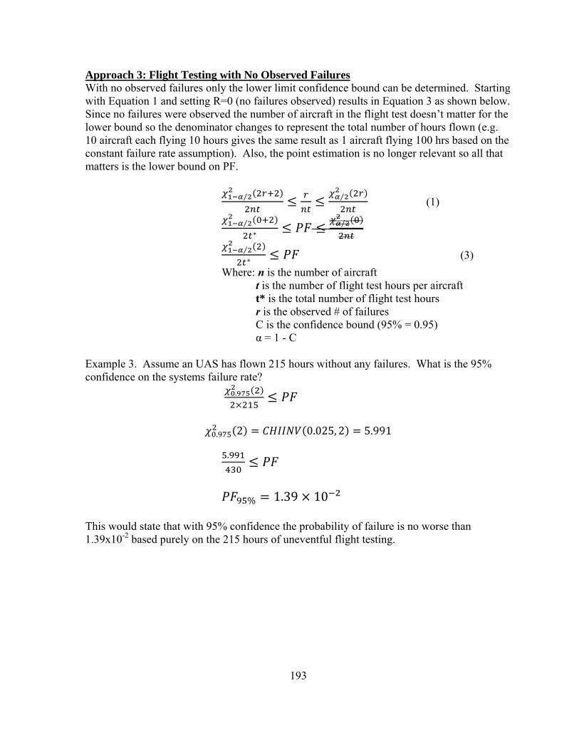
193

Approach 3: Flight Testing with No Observed Failures With no observed failures only the lower limit confidence bound can be determined. Starting with Equation 1 and setting R=0 (no failures observed) results in Equation 3 as shown below. Since no failures were observed the number of aircraft in the flight test doesn’t matter for the lower bound so the denominator changes to represent the total number of hours flown (e.g. 10 aircraft each flying 10 hours gives the same result as 1 aircraft flying 100 hrs based on the constant failure rate assumption). Also, the point estimation is no longer relevant so all that matters is the lower bound on PF.

⁄ ⁄ (1)

⁄ ⁄

⁄ (3)

Where: n is the number of aircraft t is the number of flight test hours per aircraft t* is the total number of flight test hours r is the observed # of failures C is the confidence bound (95% = 0.95) α = 1 - C Example 3. Assume an UAS has flown 215 hours without any failures. What is the 95% confidence on the systems failure rate?

.

. 2 0.025, 2 5.991

. % 1.39 10 This would state that with 95% confidence the probability of failure is no worse than 1.39x10-2 based purely on the 215 hours of uneventful flight testing.

194

Application As an example assume that some UAS has flown 22,994 flight hours and had 77 mishaps that resulted in the loss of the vehicle. Cumulative Flight Hours: 22,994 # of Class A Mishaps: 77

⁄ ⁄ (1)

Where: nt = 22,994 r = 77 α=0.05 (95% confidence)

., ,

.,

.,

3.35 10 .,

.,

3.35 10 .,

4.28 10 3.35 10 2.68 10 This shows that even with nearly 23,000 operational hours the conservative 95% confidence lower bound differs from the simple point estimation37 by almost 28%.

37 The point estimation is derived by dividing the number of mishaps by the total number of flight hours. 

95% Confidence that system failure rate is at least this good.

95% Confidence that system failure rate is no better than this.

Point estimation of failure rate.