ABSTRACT

Title of dissertation: BIO-INSPIRED INFORMATIONEXTRACTION IN 3-D ENVIRONMENTSUSING WIDE-FIELD INTEGRATIONOF OPTIC FLOW

Andrew Maxwell Hyslop,Doctor of Philosophy, 2010

Dissertation directed by: Assistant Professor J. Sean HumbertDepartment of Aerospace Engineering

A control theoretic framework is introduced to analyze an information extrac-

tion approach from patterns of optic flow based on analogues to wide-field motion-

sensitive interneurons in the insect visuomotor system. An algebraic model of optic

flow is developed, based on a parameterization of simple 3-D environments. It is

shown that estimates of proximity and speed, relative to these environments, can be

extracted using weighted summations of the instantaneous patterns of optic flow.

Small perturbation techniques are utilized to link weighting patterns to outputs,

which are applied as feedback to facilitate stability augmentation and perform local

obstacle avoidance and terrain following. Weighting patterns that provide direct

linear mappings between the sensor array and actuator commands can be derived

by casting the problem as a combined static state estimation and linear feedback

control problem. Additive noise and environment uncertainties are incorporated

into an offline procedure for determination of optimal weighting patterns.

Several applications of the method are provided, with differing spatial mea-

surement domains. Non-linear stability analysis and experimental demonstration is

presented for a wheeled robot measuring optic flow in a planar ring. Local stabil-

ity analysis and simulation is used to show robustness over a range of urban-like

environments for a fixed-wing UAV measuring in orthogonal rings and a micro he-

licopter measuring over the full spherical viewing arena. Finally, the framework is

used to analyze insect tangential cells with respect to the information they encode

and to demonstrate how cell outputs can be appropriately amplified and combined

to generate motor commands to achieve reflexive navigation behavior.

BIO-INSPIRED INFORMATION EXTRACTION IN 3-DENVIRONMENTS USING WIDE-FIELD INTEGRATION OF

OPTIC FLOW

by

Andrew Maxwell Hyslop

Dissertation submitted to the Faculty of the Graduate School of theUniversity of Maryland, College Park in partial fulfillment

of the requirements for the degree ofDoctor of Philosophy

2010

Advisory Committee:Assistant Professor J. Sean Humbert, Chair/AdvisorProfessor Rama ChellappaAssociate Professor Robert M. SannerAssociate Professor David AkinProfessor Inderjit Chopra

c© Copyright byAndrew Maxwell Hyslop

2010

Acknowledgments

Insects are pretty dumb, but I still required 7.5 years of tertiary education

to make a tiny contribution to the exciting new field of transitioning their ‘simple-

minded’ architecture to ‘intelligent’ man-made robots. Perhaps the day will arrive

when Skynet becomes self-aware and dooms us all, but we are certaintly not there

yet.

First and foremost, I want to thank my advisor, Dr. Sean Humbert, for

providing me with a challenging and inspiring topic, completely outside the realm of

my previous experience. Sean invests himself in his students with great enthusiasm

and is always full of ideas and new research directions. I would not have been able

to complete my PhD in such a short period without his flexibility, understanding

and yet firm management style. Thanks also to my lab mates for all their help; Mike

and Scott for the ground robot, David and Brian for AVLSim, Imraan for his insect

dynamics sys ID, and Joe, Greg and Badri for the quadrotor. Joe, your enthusiasm

for the Thirsty Turtle is undying, and I respect that; Greg, your Australian accent

still needs a lot of work; and Badri, you are an enigma. The Thirsty Turtle deserves

a shout out of their own, for their $1 beer pricing structure and for the mini-skirts

that just keep getting shorter.

Thanks to Mrs Fox of Gray St Primary for telling us that if we didn’t learn our

times tables we’d end up as check-out chicks at Safeway. My education also owes

thanks to space tether gurus Michiel Kruijff and Erik van der Heide, my undergrad

advisor Dr. Chris Blanksby, Ray ‘math is cool’ Peck, math-teacher-comedian Julian

ii

Grigg, and my physics teacher - the late Karen Tucker. Thanks to Mum, Dad and

Katie, for their infinite support and putting up with me living overseas to follow

a childhood dream. Thanks also to my loving girlfriend Eliane, who hates flies,

especially big Australian ones that bite. Maybe if she reads this thesis she will learn

to love them as much as she loves Echidnas. Thanks also to her family for being

great proxy parents. Finally, I want to thank America for providing research and

career opportunities that Australia could not.

iii

Table of Contents

List of Tables vi

List of Figures vii

List of Nomenclature and Abbreviations xi

1 Introduction 11.1 Visuomotor Feedback in Insects . . . . . . . . . . . . . . . . . . . . . 41.2 Optic-flow-based Navigation in Robotics . . . . . . . . . . . . . . . . 61.3 Thesis Contributions and Organization . . . . . . . . . . . . . . . . . 10

2 Wide-Field Integration of Optic Flow 122.1 Optic Flow Model . . . . . . . . . . . . . . . . . . . . . . . . . . . . . 13

2.1.1 What is Optic Flow? . . . . . . . . . . . . . . . . . . . . . . . 132.1.2 How is it Modeled? . . . . . . . . . . . . . . . . . . . . . . . . 13

2.2 Parameterization of the Environment . . . . . . . . . . . . . . . . . . 172.3 Tangential Cell Analogues . . . . . . . . . . . . . . . . . . . . . . . . 242.4 Interpreting WFI Outputs . . . . . . . . . . . . . . . . . . . . . . . . 26

3 Closed-Loop Architecture 303.1 Feedback Control Design . . . . . . . . . . . . . . . . . . . . . . . . . 313.2 Stage 1: Optimal Static Estimation of Relative States . . . . . . . . . 35

3.2.1 Measurement Model . . . . . . . . . . . . . . . . . . . . . . . 353.2.2 Weighted Least Squares Inversions . . . . . . . . . . . . . . . 36

3.2.2.1 Noise Covariance Matrix . . . . . . . . . . . . . . . . 373.2.2.2 Model Uncertainty Penalty Matrix . . . . . . . . . . 393.2.2.3 Fisher Information . . . . . . . . . . . . . . . . . . . 40

3.2.3 State Extraction Weighting Functions . . . . . . . . . . . . . . 423.3 Stage 2: Optimal Feedback Gains . . . . . . . . . . . . . . . . . . . . 43

4 Robotic Applications 454.1 1-D WFI Demonstrations . . . . . . . . . . . . . . . . . . . . . . . . 45

4.1.1 Ground Robot using Ring-constrained WFI . . . . . . . . . . 454.1.1.1 WFI-Based Controller . . . . . . . . . . . . . . . . . 454.1.1.2 Nonlinear Stability Analysis . . . . . . . . . . . . . . 474.1.1.3 Experimental Validation . . . . . . . . . . . . . . . . 514.1.1.4 Optimal Weighting Functions for Planar Vehicles with

a Nonholonomic Sideslip Constraint . . . . . . . . . 564.1.2 Quadrotor using Ring-constrained WFI . . . . . . . . . . . . . 59

4.2 2-D WFI Demonstrations . . . . . . . . . . . . . . . . . . . . . . . . 614.2.1 Fixed-Wing UAV using Ring-constrained WFI . . . . . . . . . 61

4.2.1.1 WFI-Based Controller . . . . . . . . . . . . . . . . . 624.2.1.2 Stability and Robustness Analysis . . . . . . . . . . 67

iv

4.2.1.3 Simulation . . . . . . . . . . . . . . . . . . . . . . . 684.2.2 Micro Helicopter using Spherical WFI . . . . . . . . . . . . . 74

4.2.2.1 WFI-Based Controller . . . . . . . . . . . . . . . . . 744.2.2.2 Stability and Robustness Analysis . . . . . . . . . . 814.2.2.3 Simulation . . . . . . . . . . . . . . . . . . . . . . . 84

5 Control Theoretic Interpretation of Tangential Cells 905.1 1-D Tangential Cell Directional Templates . . . . . . . . . . . . . . . 93

5.1.1 Decoding TC Patterns . . . . . . . . . . . . . . . . . . . . . . 935.1.2 Static TC Output Feedback . . . . . . . . . . . . . . . . . . . 965.1.3 Experimental Validation . . . . . . . . . . . . . . . . . . . . . 96

5.1.3.1 Feedback Synthesis . . . . . . . . . . . . . . . . . . . 965.1.3.2 Results . . . . . . . . . . . . . . . . . . . . . . . . . 98

5.1.4 Discussion . . . . . . . . . . . . . . . . . . . . . . . . . . . . . 1025.2 2-D Tangential Cell Directional Templates . . . . . . . . . . . . . . . 103

6 WFI Algorithm Summary 1116.1 WFI-Based Controller Design . . . . . . . . . . . . . . . . . . . . . . 1116.2 Real-time Algorithm Implementation . . . . . . . . . . . . . . . . . . 113

7 Summary and Conclusions 1157.1 Feasibility . . . . . . . . . . . . . . . . . . . . . . . . . . . . . . . . . 1157.2 Limitations . . . . . . . . . . . . . . . . . . . . . . . . . . . . . . . . 1167.3 Comparison with Literature . . . . . . . . . . . . . . . . . . . . . . . 1177.4 Conclusions . . . . . . . . . . . . . . . . . . . . . . . . . . . . . . . . 1207.5 Future Work . . . . . . . . . . . . . . . . . . . . . . . . . . . . . . . . 124

A Derivations 127A.1 WFI Simplification using Linearized Optic Flow Model . . . . . . . . 127A.2 Flat-Camera to Sphere Mapping . . . . . . . . . . . . . . . . . . . . . 128A.3 WFI Computation for Different Measurement Grids . . . . . . . . . . 132

Bibliography 134

v

List of Tables

2.1 Outdoor flat-surface world with no front/rear surfaces; 1-D nearness sub-functions in the roll, pitch and yaw planes . . . . . . . . . . . . . . . . . 24

4.1 Linearized 3-Ring optic flow decomposition for baseline environments . . . 634.2 Fixed-wing UAV stability characteristics . . . . . . . . . . . . . . . . . . 654.3 Inversion of Fourier outputs (to obtain static state estimates) and desired

trajectory . . . . . . . . . . . . . . . . . . . . . . . . . . . . . . . . . . 664.4 Fixed-wing UAV feedback gains . . . . . . . . . . . . . . . . . . . . . . 664.5 Micro helicopter stability characteristics . . . . . . . . . . . . . . . . . . 754.6 Micro helicopter feedback gains . . . . . . . . . . . . . . . . . . . . . . 81

5.1 Tangential cell feedback gains K for rotation rate control, using Fig.3.1B control loop architecture . . . . . . . . . . . . . . . . . . . . . . 100

5.2 Minimum estimate covariance (relative to the global optimum) as afunction of WFI weighting pattern set . . . . . . . . . . . . . . . . . 101

5.3 Minimum estimate covariance as a function of field of view . . . . . . 1015.4 Longitudinal Drosophila dynamics modes (SI units) in hover condition1045.5 Lateral Drosophila Dynamics Modes (SI units) in hover condition . . 1045.6 Spatial inner product between tangential cell directional templates

and optic flow pattern induced by natural mode motion and inputexcitation modes. . . . . . . . . . . . . . . . . . . . . . . . . . . . . . 107

5.7 Spatial inner product between positively combined (right plus lefthemisphere, normalized) tangential cell directional templates and op-tic flow pattern induced by natural mode motion and input excitationmodes. . . . . . . . . . . . . . . . . . . . . . . . . . . . . . . . . . . . 108

5.8 Spatial inner product between negatively combined (right minus lefthemisphere, normalized) tangential cell directional templates and op-tic flow pattern induced by natural mode motion and input excitationmodes. . . . . . . . . . . . . . . . . . . . . . . . . . . . . . . . . . . . 109

vi

List of Figures

1.1 Autonomous Guidance, hierarchical breakdown. Yellow - strategichigh-level mission goal direction, Red - tactical maneuvering throughclutter to target, Blue - reactive obstacle avoidance maneuver thatpreempts urban or cluttered maneuvering . . . . . . . . . . . . . . . . 2

1.2 Current micro-size sensor technology. . . . . . . . . . . . . . . . . . . 31.3 Visuomotor system structure. Local motion of luminance patterns

is processed by EMDs (not shown) and communicated to the thirdvisual ganglion, where wide-field integrating neurons extract infor-mation for control and navigation. . . . . . . . . . . . . . . . . . . . . 4

2.1 Optic flow vector field superimposed on camera image. Each opticflow vector denotes the local movement in the image between Frame1 and Frame 2. . . . . . . . . . . . . . . . . . . . . . . . . . . . . . . 14

2.2 Geometry of imaging surface. Optic flow is the projected relativevelocities of objects in the environment into the tangent space Tr ofthe imaging surface - e.g., (A) a sphere S2 or (B) circular S1 rings. . 16

2.3 Environment models for nearness function approximation: (A) flat-surface world with translational perturbations, (B) ellipsoid worldwith centered vehicle, (C) outdoor obstacle-free flight (and definitionof the distance function d(γ, β,q)), (D) outdoor flight with east-sideobstacle . . . . . . . . . . . . . . . . . . . . . . . . . . . . . . . . . . 19

2.4 Nominal optic flow patterns; (A) tunnel with floor, (B) right-side wallwith floor, (C) tunnel . . . . . . . . . . . . . . . . . . . . . . . . . . . 27

2.5 WFI of optic flow in an infinite tunnel. The optic flow field is mea-sured (represented here using ‘bug eyes’) then integrated over thesphere against a weighting pattern to produce a scalar output. Spher-ical harmonics up to 2nd degree are sufficient to obtain relative mea-surements of all navigational and stability states in this simple en-vironment. Undesired asymmetries in the optic flow pattern can beeliminated by applying these quantities as feedback to appropriateactuators, thus forcing the vehicle to track a symmetric pattern (Fig.2.4C). . . . . . . . . . . . . . . . . . . . . . . . . . . . . . . . . . . . 29

3.1 Equivalent closed-loop architectures; (A) direct feedback of carefullyselected WFI outputs, (B) gained feedback of arbitrary WFI outputs,(C) state extraction from arbitrary WFI outputs and state feedback . 32

3.2 Equivalent closed-loop architecture with explicit state estimation;gained feedback of carefully selected WFI outputs . . . . . . . . . . . 43

4.1 (A) Environment approximation with planar vehicle, (B) nominal 1Doptic flow as function of viewing angle, (C) nominal equatorial opticflow field around insect in an infinite tunnel. . . . . . . . . . . . . . . 46

vii

4.2 Contour plots of V and V and the regions D = R1 ∪R2 ∪R3 (whereV < 0) and D′ (for which asymptotic stability is guaranteed); (A)K1 = −24, K2 = 13 (gains used in 4.1.1.3), (B) K1 = −2.4, K2 = 0.13. 50

4.3 Information flow diagram for ground vehicle; x = (u, y, ψ), u =ur, uu, and uref = K3Nuref , 0. . . . . . . . . . . . . . . . . . . . 51

4.4 (A) Ground vehicle configuration, (B) Camera view with an examplering used for 1D optic flow extraction, and (C) Tunnel wall texture. 52

4.5 Centering response in a 90 corridor for a fixed forward speed; (A)ground vehicle and wall textures, (B) trajectories (and mean) for 20trials with a combined 0.25 m lateral and 45 orientation offset, (C)first ya1 and second ya2 cosine harmonics (WFI outputs), and means,for the 20 trials, (D) trajectories for different initial lateral offsets (0,5, 10, 15 in.) and (E) orientation offsets (0, 30, 60, 80), (F) opticflow pattern Q(γ) measured at time t = tF and (G) at t = tG. . . . . 54

4.6 Clutter response for 20 trials; (A) converging-diverging tunnel envi-ronment, (B) trajectories and mean, (C) forward speed u and firstsine harmonic yb1 (WFI output) as a function of tunnel position forthe 20 trials along with the mean. . . . . . . . . . . . . . . . . . . . . 56

4.7 Schematic diagram of quadrotor components. . . . . . . . . . . . . . 604.8 Fixed-wing UAV with ring-constrained optic flow sensing. . . . . . . . 614.9 Root locus diagrams for range of environments and obstacle spacings.

Closed-loop eigenvalues computed for a up to 1000 m (∼ ∞) in stepsof 0.5 m. A ’no obstacles’ environment is obtained when a →∞. . . . 68

4.10 3-D simulation environments; (A) single wall, (B) tunnel with 20

ramp and 30 bend. . . . . . . . . . . . . . . . . . . . . . . . . . . . . 694.11 Optic flow sampling regions. Cameras form panoramas in 3 orthogo-

nal planes, but optic flow is only measured in the mid-line regions ofthe panoramas. . . . . . . . . . . . . . . . . . . . . . . . . . . . . . . 70

4.12 Ring-constrained WFI simulation process diagram. . . . . . . . . . . 714.13 Simulation results - trajectories. (A) Single wall (initial ψ = 0, 15, 30, 45):

plan view; (B) tunnel with 20 ramp and 30 bend (initial y = 2, z = 2m,ψ = 15): i) side view, ii) plan view. (C) tunnel (initial y =−4,−2, 2, 4 m): plan view; (D) tunnel (initial z = −5,−2.5, 2.5, 5m): side view. . . . . . . . . . . . . . . . . . . . . . . . . . . . . . . . 72

4.14 Simulation results for tunnel environment (initial y = 2, z = 2 m,ψ =15): speeds, rates and optic-flow-extracted measurements. . . . . . . 72

4.15 Simulation results for tunnel environment (initial y = 2, z = 2 m,ψ =15): configuration states and optic-flow-extracted measurements.Note: ‘w.r.t.’ denotes ‘with respect to’. . . . . . . . . . . . . . . . . . 73

4.16 Optimum weighting patterns to recover environment-scaled statesfrom optic flow field. . . . . . . . . . . . . . . . . . . . . . . . . . . . 77

4.17 Optimum weighting patterns to recover environment-scaled statesfrom optic flow field, restricted to lower hemisphere measurements. . 79

4.18 Optimum weighting patterns to extract stabilizing control commandsfrom optic flow field. . . . . . . . . . . . . . . . . . . . . . . . . . . . 82

viii

4.19 Root locus diagram for range of wall spacings. Closed-loop eigenval-ues computed for aW and aE independently ranging from 1 m to 1000m (∼ ∞) in steps of 1 m. . . . . . . . . . . . . . . . . . . . . . . . . . 83

4.20 3-D simulation environment. . . . . . . . . . . . . . . . . . . . . . . . 854.21 Sampling the optic flow field: projections of camera boundaries on to

right and left hemispheres of the sphere. . . . . . . . . . . . . . . . . 854.22 Spherical WFI simulation process diagram. . . . . . . . . . . . . . . . 864.23 Simulation results - trajectories (Part 1). (A) Plan view of all tra-

jectories using full spherical measurement grid, (B) alternate view oftrajectories. . . . . . . . . . . . . . . . . . . . . . . . . . . . . . . . . 87

4.24 Simulation results - trajectories (Part 2). (C) Plan view comparisonbetween spherical measurement grid and half-sphere grid for a singleinitial condition, (D) side view comparison during navigation over a0.5 m box, (E) 1 m box, (F) 1 m ramp. . . . . . . . . . . . . . . . . . 88

4.25 Speeds, rates and optic-flow-extracted measurements for the full spher-ical measurement grid case (Fig. 4.23C) during a 90 turn. . . . . . . 88

4.26 Vehicle pose, WFI outputs and measured optic flow for the full spher-ical measurement grid case (Fig. 4.23C during a 90 turn. . . . . . . 89

5.1 Directional templates of right brain hemisphere Calliphora tangentialcells sensitive to primarily horizontal optic flow. . . . . . . . . . . . . 91

5.2 Directional templates of right brain hemisphere Calliphora tangentialcells sensitive to primarily vertical optic flow. . . . . . . . . . . . . . . 92

5.3 Extraction of equatorial-azimuthal flow sensitivity for a left and righthemisphere tangential cell; (A) 2-D directional templates (data ex-tracted and replotted from [1, 2, 3]), (B) azimuthal flow componentfor equatorial ring. . . . . . . . . . . . . . . . . . . . . . . . . . . . . 94

5.4 State extraction pattern Fx = C†F comparison for control-relevantstates and three different tangential cell weighting function set selec-tions. . . . . . . . . . . . . . . . . . . . . . . . . . . . . . . . . . . . . 97

5.5 Direct optic flow to actuator pattern Fu = KC†Fy comparison forthree different tangential cell weighting function set selections. . . . . 98

5.6 Cluttered obstacle field environment. . . . . . . . . . . . . . . . . . . 995.7 Vehicle trajectories (10 trials) and mean trajectory for tunnel with

90 bend and a cluttered obstacle field (forward speed u0 = 0.4 m/s);tangential cell gains determined from (A,D) 4-cell LS, (B,E) 16-cellLS, (C,F) 16-cell MV . . . . . . . . . . . . . . . . . . . . . . . . . . . 99

5.8 Optic flow patterns induced by natural mode motion and input exci-tation modes; dynamics model: Drosophila in hover condition; envi-ronment model: sphere, 1 m radius. (A) Longitudinal natural modes,(B) longitudinal input excitation modes, (C) lateral natural modes,(D) lateral input excitation modes. . . . . . . . . . . . . . . . . . . . 106

ix

7.1 AVLSim comparison of optimal WFI weighting pattern methodol-ogy to a typical left vs right patch comparison scheme (with removalof rotation-component from the optic flow). Measurements are re-stricted to the upper hemisphere to avoid sensing the floor. (A)Weighting patterns mapping optic flow measurements to rotation ratecommand, (B) wheeled robot trajectories through a corridor with 90

bend . . . . . . . . . . . . . . . . . . . . . . . . . . . . . . . . . . . . 1197.2 Centeye, IncTMMAOS; will deliver optic flow measurements over the

entire sphere . . . . . . . . . . . . . . . . . . . . . . . . . . . . . . . . 126

A.1 Projection of spherical coordinate grid on to flat imaging surface.Shown is an equatorial measurement node projected from the unitsphere to the camera surface along vector r. The surface boundariesare defined by the horizontal and vertical field of views. . . . . . . . . 130

x

Nomenclature

A state space dynamics matrixa lateral obstacle clearance, mB control coefficients matrixB body frameC observation matrixC camera frameC correlation matrixc cosine functionC† observation inversion matrixd distance, mF weighting patternF inertial fixed frameF Fisher information matrixg front/rear obstacle clearance, mh vertical obstacle clearance, mJ LQR performance indexK gain matrixK number of measurement pointsL local frame on sphere surfaceM number of outputsN normalization coefficientn number of statesP state estimate covariance matrixP number of actuatorsp roll rate, rad/s

Q optic flow, rad/sq vehicle poseq pitch rate, rad/sR noise covariance matrixR rotation matrixr point on imaging surfacer yaw rate, rad/ss sine functionT kinematic transform matrixu control vector (trim perturbation)u forward velocity, m/sv velocity vector, m/sv modal vectorv lateral velocity, m/sW output weighting matrixw WFI measurement noise vectorw vertical velocity, m/sx vehicle state vector

x forward offset, mY spherical harmonic functiony WFI outputs, rad/sy lateral offset, mz vertical offset, mα field of view, radβ body-referred elevation angle, radγ body-referred azimuth angle, radδ perturbationδa = aileron deflection from trim, radδe = elevator deflection from trim, radδr = rudder deflection from trim, radδT = thrust offset from trim, Nε weighting of model uncertainty termη optic flow measurement noise vectorθ pitch angle, radµ nearness function, 1/mΛ normalized actuator inputξ lateral flapping angle, radΦ Legendre functionφ roll angle, radχ longitudinal flapping angle, radψ heading angle, radΩ solid angle, srω angular rate vector, rad/s

Additional Subscripts/Superscriptsam order m sine harmonicb body framebm order m cosine harmonicc camera frameD inertial down directionE inertial EastH horizontalL left brain hemispherel harmonic degreelat laterallin linearizedlon longitudinalm harmonic ordermr main rotorN inertial Northnl = nonlinear

xi

P = pitch planeR = roll planeR right brain hemisphereref reference/target trajectoryS inertial Southt thrustU inertial up directionV verticalW inertial WestY = yaw plane˜ measured quantityˆ estimated quantity0 nominal

AbbreviationsDOF Degrees Of FreedomEMD Elementary Motion Detector

FPS Frames Per SecondFOV Field Of ViewGPS Global Positioning SystemHS Horizontal SystemIMU Inertial Measurement UnitLS Least Squares EstimatorLQR Linear Quadratic RegulatorMAOS Multiaperture Optical SystemMAV Micro Air VehicleMV Minimum Variance EstimatorTC Tangential CellUAV Uninhabited Air VehicleVLSI Very-Large-Scale IntegrationVS Vertical SystemWFI Wide-Field Integration

xii

Chapter 1

Introduction

Current uninhabited air vehicles (UAVs) are equipped with sensors that enable

the platform to maintain stable flight, track a desired flight trajectory, and perform

strategic-level waypoint navigation via GPS (yellow trajectory in Fig. 1.1). How-

ever, they do not permit operation around local unmapped obstacles, such as trees

and buildings inside a city. Whilst some candidate technologies exist to potentially

perform this task, they do not scale down to the stringent payload requirements

of micro air vehicles (MAVs), a physically miniature subclass of UAVs. It is the

aim of this thesis to help bridge the gap between the the available sensor technolo-

gies and the type of missions and navigational capabilities desired for the MAVs.

Specifically, the intent is to leverage sensing concepts from the insect visuomotor

system to provide the proximity and velocity information required for tactical level

navigation (red trajectory in Fig. 1.1).

Interest in micro air vehicle (MAV) platforms has expanded significantly in

recent years, primarily due to the requirement for inexpensive surveillance and re-

connaissance in potentially inaccessible or dangerous areas. To be truly effective,

these platforms will need to be endowed with the capability to operate autonomously

in unmapped obstacle-rich environments. Whilst significant investment and progress

has been made in the areas of actuation and fabrication technology for micro-scale

1

Figure 1.1: Autonomous Guidance, hierarchical breakdown. Yellow - strategic high-level mission goal direction, Red - tactical maneuvering through clutter to target,Blue - reactive obstacle avoidance maneuver that preempts urban or cluttered ma-neuvering

systems [4, 5, 6, 7], sensors, processing, and feedback control architectures are dra-

matically behind the curve at these scales.

The fast dynamics of these MAVs call for high bandwidth sensors, and the

payload limitations dictate a sensor suite on the order of 1 g, consuming less than 1

mW of power. Existing guidance systems consistent with small payloads (Fig. 1.2)

are low bandwidth (5 Hz), weigh on the order of 15-30 g, require 0.75-1 W of power,

and do not function indoors due to GPS availability. Miniature laser rangefinders

[8] and ultrasonics have the required bandwidth, however implementations are also

on the order of 25-40 g, require 400 mW, and have a very limited field of view

(FOV). Traditional machine vision approaches [9, 10, 11, 12, 13, 14, 15, 16] that infer

proximity and velocity information from camera imagery have been demonstrated,

however these algorithms are computationally expensive and require off-board visual

processing, even on vehicles with significant payloads [17]. For an aerial microsystem

with a requirement of both indoor and outdoor operation, there are currently no

2

Figure 1.2: Current micro-size sensor technology.

viable approaches to achieve the required velocity estimation, obstacle localization

and avoidance [18, 19]. Hence, novel sensors and sensory processing architectures

will need to be explored if autonomous microsystems are to be ultimately successful.

For inspiration, researchers are looking to the millions of examples of flying

insects that have developed elegant solutions to the challenges of visual perception

and navigation [20]. Insects rely on optic flow [21, 22], the characteristic patterns of

visual motion that form on their retinas as they move. These time dependent motion

patterns are a rich source of visual cues that are a function of the relative speed and

proximity of the insect with respect to objects in the surrounding environment [23].

The insect’s visuomotor system performs computations in a very small volume, and

manages the rapid convergence of signals from thousands of noisy motion detectors

to a small number of muscle commands. The robust flight behaviors that result [24,

25, 26, 27] align well with the capabilities desired for MAVs. To effectively leverage

this concept, the relevant information processing techniques must be formalized and

linked, via feedback, to the navigational heuristics observed by behavioral biologists.

3

Photoreceptors

Lobula

Plate

Tangential

Cell

Lobula

Descending

Cell

Figure 1.3: Visuomotor system structure. Local motion of luminance patterns isprocessed by EMDs (not shown) and communicated to the third visual ganglion,where wide-field integrating neurons extract information for control and navigation.

Therefore, the central aim of this thesis is to formulate the fundamental estimation

and control principles for transition of this biologically-inspired architecture to 6-

DOF engineered systems.

1.1 Visuomotor Feedback in Insects

The insect retina, composed of thousands of individual sub-units, functions

to image the incident patterns of luminance from the environment. As an insect

moves, the intensity of the image formed at each lens becomes time dependent.

The rate and direction of the local image shifts, taken over the entire field of view,

form patterns of optic flow. The spatial structure of the patterns of optic flow

that the insect experiences is governed primarily by the insect’s relative motion and

4

proximity to objects through motion parallax, a relationship that can be expressed

mathematically in closed form [28]. Extraction of visual information contained in

optic flow is performed by wide-field sensitive tangential cells, which communicate

their output through descending neurons to the flight motor to execute changes in

wing kinematics [21, 22].

The tangential cells are large, motion-sensitive neurons that reside in the lob-

ula plate portion of the third visual ganglia (Fig. 1.3). They are believed to integrate

(pool) the outputs of large numbers of retinotopically distributed elementary motion

detectors (EMDs) [29, 30, 2, 21, 22]. Prominent among the tangential cells are the

identified neurons that comprise the ‘horizontal system’ (HS) and ‘vertical system’

(VS) found in a number of species of flies [31, 32, 33]. As their names suggest,

these neurons are sensitive primarily to horizontal and vertical patterns of optic

flow, respectively. They respond with graded membrane potentials whose polarity

depends on the direction of motion. Their spatial sensitivity to local motion cues

has in some cases been mapped out [2], as shown for several cells in Figs. 5.1 and

5.2, and the resemblance of some of these maps to the patterns of optic flow induced

by particular modes of egomotion has led to the hypothesis that the correspond-

ing neurons may act as matched filters for these patterns [34, 35]. However, recent

work has shown that translational motion cues, which are the source of proximity

information, are also present in the outputs of cells that were previously thought to

be used only for compensation of rotary motion [36]. This suggests that cell pat-

terns might be structured to extract a combination of relative speed and proximity

cues, rather than direct estimates of the velocity state. Hence, while some progress

5

has been made in understanding structure, arrangement, and synaptic connectivity

[21], the exact functional role that the tangential cells hold in the stabilization and

navigation system of the fly remains a challenging and open question.

1.2 Optic-flow-based Navigation in Robotics

The idea that insects use optic flow to navigate has inspired a number of

studies in the robotics field. This section describes research in closed-loop optic-

flow-based navigation and egomotion estimation, and introduces the concept of wide-

field integration (WFI), a technique based on the visuomotor principles discussed

in Section 1.1.

In most studies that attempt closed-loop obstacle avoidance using optic flow,

a feedback signal is generated by comparing single points or uniformly averaged

patches of optic flow on the sides or the bottom of a vehicle to generate a control

input. Navigational goals included obstacle navigation [37, 38, 39, 40, 41, 42, 43, 44,

45, 46], speed control [47, 48, 49, 50] and terrain following [51, 52, 53]. These efforts

provide a path forward, but they generally ignore (in favor of more traditional

architectures) the fundamental processing and feedback mechanisms that insects

employ to extract information from optic flow and to regulate behavior. Some

studies required independent sensing of vehicle rotation rates or nulling of the sensor

during rotation maneuvers, and results are predominately presented without formal

closed loop stability analysis.

In more academic approaches, algorithms have been applied to generate esti-

mates of egomotion and/or the structure of objects in the surrounding environment

6

based on optic flow measurements. Past research typically involves fitting a theo-

retical model of optic flow to measurements at a series of points in a camera image

by numerical solution of the least squares problem [54, 55, 56, 57]. With the as-

sumption of forward-dominated motion, it is possible to resolve the direction of a

vehicle’s velocity vector, its rotation rates and a 3-D depth map [58]. Fast Fourier

Transforms can be employed to speed up computations, but the process still requires

∼1 s on a Pentium processor. One can also simplify the problem by using an initial

estimate of egomotion (from IMU/GPS) to extract terrain shape [59] and then, at

the next update, extract egomotion using the terrain shape estimate [54, 60] and so

on. Noise reduction is often achieved by only measuring optic flow at high contrast

image points, which provides more accurate estimates but requires a feature detec-

tion step [61, 55, 62, 60]. To further smooth estimates, the dynamics of the vehicle

can be incorporated by using extended Kalman filters, with the nonlinear optic flow

equations forming the measurement model [63, 62, 10] and with optional fusing of

IMU data [64]. Whilst these algorithms may be feasible for implementation on a

UAV with a powerful micro-processor, they do not align with the computational

constraints of MAVs. Furthermore, the above studies do not address the obstacle

avoidance task and often require an accurate model of the vehicle or environment

[54, 55, 60].

The potential of the insect visuomotor architecture to provide egomotion es-

timation at low computation cost was first explored in detail by Franz and Krapp

[35]. In this study, a linear algorithm was derived, based on the idea that tangential

cells integrate the measured motion field against a pre-stored weighting pattern. By

7

selecting weightings that match the apparent motion induced by particular modes of

egomotion, one can filter the measured optic flow field to extract quantities of inter-

est. However, the matched filters required a post-processing stage and there was no

attempt to extract proximity cues or close the navigation loop. These shortcomings

were addressed by Humbert et al. [65, 66, 67, 68], who developed a mathematical

framework to analyze the insect’s approach, termed Wide-Field Integration [68].

The concept is based on static feedback which generates compensatory commands

to hold simple patterns of optic flow fixed on an imaging surface, such as the typical

sine wave pattern induced on a circular sensor by forward motion in a corridor.

Weighted summations of optic flow measurements are used to detect spatial imbal-

ances, shifts, and magnitude changes which have interpretations of relative proximity

and speed with respect to obstacles. An example of this approach has been observed

in the landing behavior of honeybees; a simple feedback loop which holds the ratio

of forward speed to height constant while descending toward a surface guarantees

an exponentially decaying approach trajectory [69], without the knowledge of abso-

lute speed or distance. Complicated patterns of optic flow can therefore be rapidly

decomposed into compensatory motor commands that maneuver the vehicle safely

between obstacles.

The primary advantage of WFI is computational simplicity; it does not require

direct vehicle state estimation, visual feature detection, extraction, or classification.

Useful information for stability augmentation and navigation is obtained by ana-

logues to tangential cell processing, i.e., computing a handful of inner products of

optic flow. This is a very efficient process that is extremely robust to noise, and

8

does not require high resolution visual imagery. It has been recently demonstrated

that this approach can be implemented real time in analog VLSI at high bandwidth

(5 KHz) using basic Reichardt-type elementary motion detectors (EMDs) for optic

flow estimation and a programmable current matrix for computing inner products

[70]. These sensors consume power on the order of microwatts, and can be packaged

on the order of milligrams. Therefore, WFI offers orders of magnitude improvement

in bandwidth, power consumption, and payload weight over implementations of tra-

ditional methodologies described above, which are constrained to operate on digital

processors.

In summary, the motivation for the research is to develop sensing concepts

that will allow MAVs to obtain the proximity and velocity information they need

to operate around local unmapped obstacles. Active sensing technologies do not

fit the MAVs payload constraints, therefore researchers are looking to passive tech-

niques, such as vision. Unfortunately, state-of-the-art vision algorithms to compute

egomotion and/or obstacle maps are too computationally intensive for an MAV mi-

cro processor. However, optic flow sensing, combined with wide-field integration

(inspired by the insect visuomotor system) to extract navigational quantities, can

be implemented on analog VLSI chips, providing a feasible solution. The primary

research gap which this thesis seeks to fill is the lack of a robust formal method

for designing WFI weighting patterns, which map data from a spatially distributed

sensor array to actuator commands that stabilize the vehicle and allow navigation

of obstacles.

9

1.3 Thesis Contributions and Organization

Though the tangential cell analogue (WFI) is well defined and has been sim-

ulated for simple planar platforms using 1-D optic flow measurements [65, 66, 67],

maturation of the concept requires development in several areas. In this thesis, ex-

perimental demonstrations are performed and previous stability analysis is expanded

to include non-linear dynamics and measurements. WFI theory is extended to 2-D

optic flow measurements in order to control 6-DOF vehicles in 3-D environments.

Robustness aspects are addressed by examining stability in the face of an uncer-

tain environment structure and by incorporating this uncertainty and measurement

noise properties in the design of optimal WFI weighting patterns. Finally, a control

theoretic framework is used to analyze the weighting patterns ingrained in insect

tangential cells with respect to the information they encode, and to show how they

can be used to achieve the impressive closed-loop behaviors observed by biologists.

Chapter 2 introduces an optic flow model and a tangential cell analogue, which

is used to extract navigationally relevant information from spatial patterns of the

optic flow. It is further shown how the choice of WFI weighting pattern links to

information content. Chapter 3 addresses feedback design and describes how the

problem of selecting an optimal weighting pattern can be cast as a combined static

state estimation and linear feedback control problem. The derived methodology is

applied to robotic platforms in Chapter 4, with experimental demonstrations and

simulations, and is used to analyze insect tangential cells in Chapter 5. Chapter 6

summarizes the WFI algorithm and provides a step-by-step method for real-time

10

implementation. Conclusions, limitations and areas for future work are discussed in

Chapter 7.

11

Chapter 2

Wide-Field Integration of Optic Flow

This chapter seeks to mathematically formalize the concept of WFI (the in-

formation extraction technique derived from the insect visuomotor system) in 3-D

environments. Previous efforts have either been limited to simplified planar envi-

ronments or have applied WFI without supporting analysis.

The central idea is that if one can model how navigationally relevant infor-

mation is encoded in patterns of optic flow, then one can design appropriate WFI

weighting patterns to decode the measurements. To achieve this goal, an inner prod-

uct model for tangential cell analogues is presented and a framework is introduced

to characterize the information that can be extracted from patterns of optic flow

on various measurement domains. An algebraic model of optic flow is developed by

parameterizing a family of typical 3-D environments. Offline WFI with the optic

flow model, combined with small perturbation techniques, provides linkages between

measurement weighting patterns and WFI outputs, which are functions of relative

proximity and velocity with respect to the parameterized environments.

12

2.1 Optic Flow Model

2.1.1 What is Optic Flow?

Optic flow is the apparent visual motion that one experiences when they move

through an environment. It can be thought of as the local rate and direction of

movement in an image. It is typically computed by comparing two successive frames

from a camera image sequence (e.g., Fig. 2.1) and applying an optic flow estimation

algorithm.

2.1.2 How is it Modeled?

The (true) optic flow is the vector field of relative velocities of material points

in the environment projected into the tangent space of the imaging surface (e.g., Fig.

2.2). It is a combination of the observer’s rotational and translational motion, along

with the relative proximity to surrounding objects. For a given angular velocity ω

and translational velocity v of the vantage point, along with the nearness function

µ which represents the distribution of objects in the surrounding environment, the

optic flow pattern Q on a spherical imaging surface S2 for an arbitrary distribution

of obstacles can be expressed [28] as

Q = −ω × r− µ [v − 〈v, r〉r] . (2.1)

The quantity Q = Qγ eγ + Qβ eβ has components in the azimuth γ ∈ (0, 2π) and

elevation β ∈ (0, π) directions (Fig. 2.2A), and lives in the vector-valued space of

13

Frame 1

Frame 2

Figure 2.1: Optic flow vector field superimposed on camera image. Each optic flowvector denotes the local movement in the image between Frame 1 and Frame 2.

14

square integrable functions on the sphere

L2(S2,R2) =

f =

f1(r)

f2(r)

: r ∈ S2, fk(r) ∈ L2(S2), k = 1, 2

. (2.2)

The nearness µ is equal to 1/d(γ, β,q), where d ∈ (0,∞) is the distance from the

imaging surface to the nearest object in the environment along the direction er (Fig.

2.3C) through a point on the imaging surface r(γ, β). If one expresses the velocity

v = (u, v, w) and angular velocity ω = (p, q, r) in coordinates of the body frame

B = exb, eyb

, ezb, the expressions for the azimuthal and elevation components of

optic flow are given by

Qγ = p cos β cos γ + q cos β sin γ − r sin β + µ(u sin γ − v cos γ)

Qβ = p sin γ − q cos γ + µ(−u cos β cos γ − v cos β sin γ + w sin β). (2.3)

The complete surface of the sphere represents the maximum measurement

domain possible, but navigational quantities of interest can also be decoded from

optic flow sampled over much smaller domains. One such example, that simplifies

(2.3), comprises measurement of tangential and normal (off-axis) components of

optic flow in three orthogonal and concentric circular rings (Fig. 2.2B) aligned, for

convenience, with the body-fixed axes of the 6-DOF vehicle, i.e., the roll plane R

(γ = π/2), pitch plane P (γ = 0), and yaw plane Y (β = π/2). In this case, (2.3)

15

TrS2

r (°; ¯)

r

!b

Gv

Roll Ring

R

R

R

Pitch Ring

Yaw Ring

P

Y

r (°; ¯)

r

TrS1

A

B

L

L

Figure 2.2: Geometry of imaging surface. Optic flow is the projected relative veloc-ities of objects in the environment into the tangent space Tr of the imaging surface- e.g., (A) a sphere S2 or (B) circular S1 rings.

16

simplifies to the ring-specific equations

Roll (R)

QβR = p + µR(−v cos β + w sin β)

QγR = q cos β − r sin β + µRu

Pitch (P )

QβP = −q + µP (−u cos β + w sin β)

QγP = p cos β − r sin β − µP v (2.4)

Yaw (Y )

QβY = p sin γ − q cos γ + µY w

QγY = −r + µY (u sin γ − v cos γ),

where β ∈ (0, 2π) and µk represents the nearness function constrained to plane k.

The ring-constrained optic flow lives in the vector-valued space of square integrable

functions on the circle

L2(S1,R2) =

f =

f1(r)

f2(r)

: r ∈ S1, fk(r) ∈ L2(S1), k = 1, 2

. (2.5)

2.2 Parameterization of the Environment

In order to completely specify the optic flow pattern (2.3) in closed form, sim-

plifying assumptions are required on the shape of the nearness function µ(γ, β,q) ∈

L2(S2). The nearness encodes the vehicle’s relative pose q = (x, y, z, φ, θ, ψ) with

17

respect to the environment, where (x, y, z) are the coordinates of the vantage point

with respect to an inertial frame F = ex, ey, ez located at the equilibrium posi-

tion, and (ψ, θ, φ) are the 3-2-1 Euler angles representing the relative attitude of the

body frame B with respect to F .

Two baseline world types will be modelled, and the built-in parameters of

each environment can be altered to obtain a variety of other navigationally relevant

scenarios.

1. Flat-surface World. Consider the general scenario of a vehicle surrounded

by flat surfaces positioned North, East, South, West, up and down relative to

the inertial vehicle frame. The desired position of the vehicle is some nominal

location within the enclosed room. When the vehicle deviates from its nominal

position (Fig. 2.3A), the deviation is captured by the orthogonal quantities

(x, y, z). The objective is to find a model for the distance to obstacles in this

general environment.

Expressed as a vector quantity, the distance to a surface along direction er from

a point r on the sphere is d = d(γ, β,q) er, assuming that ‖r‖ ¿ ‖d(γ, β)‖.

For the surface below the vehicle (Fig. 2.3B), the altitude is denoted as hD−z.

The component of d along the direction of the fixed frame F vertical ez is

therefore given by

〈d, ez〉 = hD − z. (2.6)

To derive the general expression for µ(γ, β,q) = 1/d(γ, β,q), the vector d

18

BA

¯ d = d(°; ¯;q)

aW+ yaE¡y

hU+ z

gN ¡x

gS+ x

B

F

exbeyb

ezb

r

er

er

ey

exez

F

ez

ex

ey

hD¡ z

hD¡ z

C

a y

d = d(°; ¯;q)

D

F

B

er

exb

eyb

ey r

ezb

er

ey

exez

ag

h

Fey

exez

Figure 2.3: Environment models for nearness function approximation: (A) flat-surface world with translational perturbations, (B) ellipsoid world with centeredvehicle, (C) outdoor obstacle-free flight (and definition of the distance functiond(γ, β,q)), (D) outdoor flight with east-side obstacle

19

needs to be expressed in F coordinates for a general orientation to facilitate

the extraction of the ez component. Consider the spherical coordinate unit

vector er (Fig. 2.2) expressed in B frame coordinates

[er]B =

sin β cos γ

sin β sin γ

cos β

. (2.7)

For an arbitrary orientation of the body frame B, the components of er ex-

pressed in F coordinates are given by [er]F = R−1BF [er]B :

[er]F =

cθcψ cθsψ −sθ

sφsθcψ − cφsψ sφsθsψ + cφcψ sφcθ

cφsθcψ + sφsψ cφsθsψ − sφcψ cφcθ

−1

sβcγ

sβsγ

cβ

.(2.8)

Hence the ez component of d can be expressed as

〈d, ez〉 = d 〈 [er]F , ez 〉 = d [sβ(sφcθsγ − sθcγ) + cβcφcθ] , (2.9)

which (combining with (2.6) and µ = 1/d) yields the lower-surface nearness

function for a general pose q of the vehicle via µ(γ, β) =〈 [er]F ,ez 〉

hD−z.

This concept can easily be extended to a surface above the vehicle by taking

µ(γ, β) =〈 [er]F ,−ez 〉

hU+z. For a wall to the east of the vehicle, µ(γ, β) =

〈 [er]F ,ey 〉aE−y

.

Repeating this method for west, north and south walls, the individual µ-

20

functions can be combined to obtain a piece-wise function that describes the

nearness to surfaces when the vehicle is inside an enclosed rectangular-prism;

µ =

sβ(cψcθcγ + sγ(sφsθ − cφsψcθ)) + cβ(sφsψcθ + cφsθ)

gN − xfront wall

−sβ(cψcθcγ + sγ(sφsθ − cφsψcθ)) + cβ(sφsψcθ + cφsθ)

gS + xrear wall

sβ(cγcθsψ + sγ(sφsθsψ + cφcψ)) + cβ(cφsθsψ − sφcψ)

aE − yright wall

−sβ(cγcθsψ + sγ(sφsθsψ + cφcψ)) + cβ(cφsθsψ − sφcψ)

aW + yleft wall

sβ(sφcθsγ − sθcγ) + cβcφcθ

hD − zground

−sβ(sφcθsγ − sθcγ) + cβcφcθ

hU + zceiling

(2.10)

Parameters gN , gS, aE, aW , hD, hU represent the desired distance from the

walls at the equilibrium position. The bounds for the validity ranges of each µ

sub-function specify where the surfaces intersect, but due to their complexity

they can only be computed numerically.

2. Ellipsoid World. Consider the scenario of a vehicle inside an ellipsoid. Define

an intermediary body frame B′ attached to the vehicle but aligned with the

inertial frame F , which is offset from the vehicle by (x, y, z). The conventional

body frame B is aligned with the geometric axes of the vehicle. The kinematic

21

transforms between the frames are:

TFB′ =

1 0 0 x

0 1 0 y

0 0 1 z

0 0 0 1

TB′B =

R−1BF 03×1

01×3 1

. (2.11)

where R−1BF is given in (2.8). If the ellipse is aligned with the inertial frame, a

vector dF from the ellipsoid center to a point on the surface can be written as

dF =

b cos γF sin βF

a sin γF sin βF

h cos βF

, (2.12)

where (2b, 2a, 2h) define the ellipsoid dimensions and (γF , βF) are inertial-

frame referred azimuth and elevation angles. If transported to the B′ frame,

the vector from the vehicle center to a point on the surface is obtained from

dB′

1

= TFB′−1

dF

1

(2.13)

then the nearness µ is 1/d = 1/‖dB′‖, resulting in (2.15). Because (2.12) is

dependent on (γF , βF), expressions for these must be found. The additional

information comes from taking the body-frame vector to an arbitrary point

22

d [er]B, Eq. (2.7), and transporting into the inertial frame.

dF

1

= TFB′TB′B

d [er]B

1

. (2.14)

Equating (2.14) with (2.12), allows solution for (γF , βF) (see (2.16)). This last

step is used to solve directly for d in the flat-surface world case, because the

z-component of dF does not depend on viewing angle.

For the ellipsoid, the nearness is a continuous function of the viewing angle.

However, a closed form expression is not possible, therefore the nearness is

found by solving a non-linear equation in d (note µ = 1/d),

d =√

(c(γF)s(βF)g − x)2 + (s(γF)s(βF)a− y)2 + (c(βF)h− z)2 (2.15)

γF = tan−1

(b

a· (cθsψcγ + (sφsθsψ + cφcψ)sγ)sβ + (cφsθsψ − sφcψ)cβ + y

d

(cθcψcγ + (sφsθcψ − cφsψ)sγ)sβ + (cφsθcψ + sφsψ)cβ + xd

)

βF = cos−1

(d

h

(sφcθsγsβ − sθcγsβ + cφcθcβ +

z

d

)). (2.16)

The indoor-like environments described by (2.10) and (2.15) can be simplified

to environments useful for outdoor navigation. Flight above a flat surface with no

obstacles is modeled by the case where gN , gS, aE, aW , hU → ∞ (Fig. 2.3C). If

there is an east-side obstacle then gN , gS, aW , hU → ∞ (Fig. 2.3D), and Fig. 2.4B

shows the expected optic flow pattern for straight-and-level-flight. For a west-side

obstacle gN , gS, aE, hU → ∞, and for the case where there are obstacles on both

sides of the vehicle gN , gS, hU → ∞ and aE = aW (Fig. 2.4A). The ellipsoid world

23

can also be separated into 8 ellipsoid segments if multi-axis asymmetries are desired.

For the case where measurements are confined to three orthogonal rings (Fig.

2.2B), the nearness functions for the outdoor flat-surface worlds simplify to those

given in Tables 2.1.

Table 2.1: Outdoor flat-surface world with no front/rear surfaces; 1-D nearness sub-functions in the roll, pitch and yaw planes

Floor Right-side Wall with Floor Tunnel with Floor

µR,1c(β−φ)cθ

h−zc(β−φ)cθ

h−zc(β−φ)cθ

h−z

µR,2 0 c(β−φ)sθsψ+s(β−φ)cψa−y

c(β−φ)sθsψ+s(β−φ)cψa−y

µR,3 0 0 − c(β−φ)sθsψ+s(β−φ)cψa+y

µP,1−sθsβ+cθcφcβ

h−z−sθsβ+cθcφcβ

h−z−sθsβ+cθcφcβ

h−z

µP,2 0 0 0

µY,1 0 cθsψcγ+sγ(sφsθsψ+cφcψ)a−y

cθsψcγ+sγ(sφsθsψ+cφcψ)a−y

µY,2 0 0 − cθsψcγ+sγ(sφsθsψ+cφcψ)a+y

2.3 Tangential Cell Analogues

Insect tangential cells are believed to pool the outputs of large numbers of local

optic flow estimates and respond with graded membrane potentials whose magnitude

is both spatially and directionally selective [30, 2, 21, 22]. Essentially, the integrated

output is a comparison between the cell’s ingrained spatial directional template

(e.g., Fig. 5.1) and that of the visual stimulus (e.g., Fig. 2.4). Mathematically,

this comparison can be modeled as an inner product 〈a,b〉, analogous to the dot

product between vectors, which is an abstraction of the angle between objects a

and b. Tangential cell analogues for spherical imaging surfaces are defined here as

24

an inner product on the function space L2(S2,R2) between the instantaneous optic

flow Q and any square-integrable weighting function F = F γ eγ + F β eβ,

y = 〈Q,F〉 =

∫

S2

Q · F dΩ, (2.17)

where ‘·’ denotes the dot product in R2 and dΩ = sin β dβ dγ is the solid angle

of the sphere. This can also be thought of as a projection of Q on to F, with the

objective of decoding information about the vehicle’s relative pose q and velocity

q = (u, v, w, p, q, r) with respect to the environment. Note that the integration

domain of this inner product may be a potentially disconnected subset of the full

sphere surface.

The objective from a controls stance is to select weighting patterns F that

extract relevant information from the measured optic flow patterns to aid navigation.

One possible starting point would be the set of tangential cell directional templates

used by insects (Figs. 5.1 and 5.2). A less constrained approach involves trying

many different patterns by taking elements from an infinite basis, such as the set of

real spherical harmonics, which are orthogonal functions on L2(S2). These functions

take the form

Yl,m(β, γ) = Nml Φm

l (cos β)

cos mγ m ≥ 0

sin |m|γ m < 0

, (2.18)

where Φml (cos β) is the associated Legendre function, l, m ∈ Z, l ≥ 0, |m| ≤ l,

and the factor Nml is a normalization coefficient. The resulting wide-field integrated

25

outputs for component weighting functions Fkl,m = Y k

l,m ek, for k ∈ γ, β are then

given by

ykl,m(x) = 〈Q,Fk

l,m〉 =

∫ 2π

0

∫ π

0

Qk(x) Y kl,m sin β dβ dγ. (2.19)

2.4 Interpreting WFI Outputs

The objective is to characterize the relationship between weighting functions

F and the relative state x = (x, y, z, φ, θ, ψ, u, v, w, p, q, r) ∈ Rn encoded by WFI

outputs. This is achieved by linearizing the outputs about a nominal optic flow

pattern, which corresponds to a nominal state x0. A desired (equilibrium) optic flow

pattern is specified by a pre-defined amount of longitudinal and lateral asymmetry.

The pattern in Fig. 2.4A, for example, corresponds physically with flight centered

between obstacles and at some desired altitude above ground. This is expressed

mathematically by the nominal trajectory x0 = (0, 0, 0, 0, 0, 0, uref , 0, 0, 0, 0, 0), where

uref is the target forward speed.

To provide an intuitive illustration of the linkages between outputs and weight-

ing patterns, consider a tunnel environment with infinitely high walls, gN , gS, hU , hD →

∞ and aE = aW (Fig. 2.4C). Several spherical harmonic projections (2.19) using

this optic flow model are presented in Fig. 2.5. For example, yβ0,0 provides a measure

of the heave velocity when the signal is linearized about x0. It quantifies the good-

ness of match between the actual optic flow field and a purely longitudinal template

pattern defined by the harmonic Y β0,0, which has constant magnitude for all points

on the sphere. A climbing vehicle experiences longitudinal optic flow on both sides

26

−180 −90 0 90 1800

30

60

90

120

150

180

Nominal Optic Flow Field

azimuth (deg)

ele

va

tio

n (

de

g)

−180 −90 0 90 1800

30

60

90

120

150

180

Nominal Optic Flow Field

azimuth (deg)

ele

va

tio

n (

de

g)

BA

−180 −90 0 90 1800

30

60

90

120

150

180

Nominal Optic Flow Field

azimuth (deg)

ele

va

tio

n (

de

g)

C

Figure 2.4: Nominal optic flow patterns; (A) tunnel with floor, (B) right-side wallwith floor, (C) tunnel

27

of the vehicle and this deviation from the nominal pattern is captured by the WFI

output yβ0,0. The Y β

1,1 harmonic weights the front and rear of the vehicle strongly but

with opposite signs, thus capturing any forward-aft optic flow asymmetry (induced

by pitch-axis rotation) in the projection. The lateral offset from the tunnel center

is captured by the yγ2,2 output, which places large negative azimuthal-flow weights

on both sides of the vehicle. If the vehicle is nearer the right-side wall the optic flow

will be larger on that side (where azimuthal flow is positive) thus the WFI output

will be negative. If the left-side wall is nearer then the negative-direction azimuthal

optic flow will be stronger and the output will be positive. The positive weighting

of the optic flow at the front and rear of the vehicle acts to filter out yaw rotation

motion from the projection.

28

h _Q ; Y¯1;1 i / ¡q

Optic Flow, _Q Weighting Pattern, Fi

Right

Hemisphere

Left

Hemisphere

Pitching

Downward

Sinking

Off-Center

h _Q ; Y¯0;0 i / w

µ1

a

¶

h _Q ; Y°2;2 i / ¡y

µu0

a

¶

Lateral

Weightings

Fore/aft weightings filter out

yaw-rotation component

Figure 2.5: WFI of optic flow in an infinite tunnel. The optic flow field is measured(represented here using ‘bug eyes’) then integrated over the sphere against a weight-ing pattern to produce a scalar output. Spherical harmonics up to 2nd degree aresufficient to obtain relative measurements of all navigational and stability states inthis simple environment. Undesired asymmetries in the optic flow pattern can beeliminated by applying these quantities as feedback to appropriate actuators, thusforcing the vehicle to track a symmetric pattern (Fig. 2.4C).

29

Chapter 3

Closed-Loop Architecture

Given the WFI operation developed in Chapter 2, the control task is to syn-

thesize a control loop that stabilizes the vehicle about a desired optic flow pattern

(or trajectory). In this chapter, a linear feedback architecture is proposed and tra-

ditional engineering tools are applied to incorporate WFI into the feedback loop

in a way that minimizes computations, encompasses feedback gain optimality, and

robustness to measurement noise and environment uncertainty.

Many previous studies, using real robotic platforms, use the WFI concept to

close the navigation loop with on-board measurements of optic flow [37, 38, 39,

42, 43, 44, 45, 48, 49, 50, 52, 53]; which is generally motivated by computational

constraints of the on-board processor. The weighting patterns employed in these

experiments almost always consist of a concatenation of uniformly weighted patches

on the sphere. For example, basic obstacle navigation can be achieved by generating

a lateral steering command from a comparison of optic flow averaged over a left-

pointing camera against optic flow averaged over a right-pointing camera (e.g., Fig.

7.1A). Some studies generate a climb rate command by regulating averaged optic

flow on a down-pointing camera to a desired reference level for terrain following.

Whilst these architectures are consistent with that proposed in this thesis (Fig.

3.1), the utilized weighting patterns are designed by trial and error and often require

30

removal of rotation motion from the optic flow field. There is scope for optimization

of these patterns by considering the signal information content generated by the

WFI operations, and this chapter seeks to exploit that.

3.1 Feedback Control Design

This section states the general form of the control law that will be utilized

throughout the thesis, and introduces equivalent expanded versions that aid the de-

sign process. To maintain simplicity, and to fit with the low computations paradigm,

only linear static compensators shall be considered. The most computationally ef-

ficient feedback methodology (Fig. 3.1A) would involve a single WFI operation per

actuator, such that the WFI output is an actuator input command uk;

uk = 〈Q,Fuk〉+ uk,ref +

∑s

Kk,ysys. (3.1)

Additional terms are included to account for intended deviation from the trim point

x0 (via control uk,ref) and feedback of non-WFI-based sensor outputs ys. Note that

u already represents the perturbation from trim input.

Choosing sensor-to-actuator weightings Fukthat stabilize the vehicle is non-

trivial, but the problem can be simplified by beginning with fixed weightings Fyj

(e.g., tangential cell patterns or spherical harmonics) and then applying static linear

feedback to the WFI outputs yj (Fig. 3.1B);

uk =∑

j

Kk,yj〈Q,Fyj

〉+ uk,ref +∑

s

Kk,ys ys. (3.2)

31

B

A

C

Optic Flow

Estimation

Plant

Dynamics

_x = f(x; u)

u

x

h _Q;Fuki

¹ Environment

Wide-Field

Integration¹K

uref

+

_Q

Optic Flow

Estimation

Plant

Dynamics

u x

yj = h _Q;Fyji

¹ Environment

Wide-Field

Integration

y = Cx

¹K

Output

Feedback

u = ¹Ky+ uref

uref

+

_Q

Optic Flow

Estimation

Plant

Dynamics

u x

K

yj = h _Q;Fyji

¹ Environment

Wide-Field

Integration

y = CxStatic

Estimator

x = Cyy

State

Feedback

Cy

x

u = K(x¡ xref)

xref

+¡ +

_Q

Figure 3.1: Equivalent closed-loop architectures; (A) direct feedback of carefullyselected WFI outputs, (B) gained feedback of arbitrary WFI outputs, (C) stateextraction from arbitrary WFI outputs and state feedback

32

The gain matrix K can be designed using existing tools such as output LQR and

then the computationally efficient control law (3.1) can be recovered by setting

Fuk=

∑j

Kk,yjFyj

, (3.3)

due to linearity of the WFI operator. Here, Fyjhas entries of zeroes for non-WFI-

based outputs.

If there are more WFI measurements than states then the system is overdeter-

mined, permitting further optimization by preferential weighting of measurements.

Such optimization can reduce noise throughput in the sensor to actuator mapping

and increase robustness to uncertainty in the environment structure. However, out-

put LQR [71], for example, does not readily incorporate preferential measurement

weighting. Therefore, we introduce an additional step in the control design process;

the WFI outputs are first converged to static estimates of state xi via a weighted

least squares inversion, then any state feedback matrix design tool can be used to

map the state estimates to actuator commands. The fixed-perturbation from trim,

which determines the desired behavior of the vehicle, can also be more intuitively

specified as a state vector, xref . Assuming additionally that the non-WFI-based sen-

sors provide direct measurements of states, the revised control law is (Fig. 3.1C):

uk =∑

i

Kk,xi

(∑j

(C†

i,j〈Q,Fyj〉)− xi,ref

)+

∑s

Kk,xs(xs − xs,ref). (3.4)

33

This is equivalent to (3.1) with the weighting pattern choice

Fuk=

∑i

Kk,xi

∑j

C†i,jFyj

(3.5)

and the fixed-perturbation from trim uk,ref = −∑i Kk,xi

xi,ref .

The above method addresses the problem of designing Fukby separating it

into tractable engineering problems for which solutions are already available. Fig.

3.1A illustrates the architecture intended for real-time implementation, whilst archi-

tectures B and C are equivalent forms that allow the application of traditional tools;

non-WFI sensor feedback was omitted to avoid clutter of the diagrams. Note that

architecture 3.1B could also be implemented in real-time if the weighting patterns

were fixed (e.g., as is the case for an insect). Equivalence between architectures is

true if the following relations hold:

Fu = KFy

K = KC† (3.6)

uref = −Kxref ,

where Fu is a matrix of actuator weighting patterns and Fy is a matrix of arbitrary

weighting patterns used to begin the control synthesis process. Optimality of the

designed actuator weighting patterns is partly dependent on Fy, but this will be

explored in Section 3.2.2.3.

34

3.2 Stage 1: Optimal Static Estimation of Relative States

Optic flow cannot be measured directly, it must be inferred from the spatiotem-

poral patterns of luminance incident on an imaging surface. Therefore, the optic

flow estimation process introduces error in the measurements, which is compounded

by sensor noise and contrast/texture variations occurring in the environment. Addi-

tional uncertainty associated with the nearness function is present due to variation

in the obstacle distributions from the baseline environments assumed in Section 2.2.

In this section an offline procedure for designing a static estimator C† that accounts

for these uncertainties in the optic flow model (2.3) and environment, e.g., (2.10), is

developed. This is the first step in the synthesis of (3.4), which is an intermediary

for constructing the computationally efficient control law (3.1).

3.2.1 Measurement Model

Given M ≥ n linearly independent weighting functions Fy = Fyj, j =

1, . . . , M, WFI outputs (2.17) using the optic flow model (2.3) can be linearized

for small perturbations about x0, which will yield linear output equations of the

form y = Cx. Accounting for environment uncertainty and measurement noise, the

observation equation becomes

y = Cx + w (3.7)

C = C0 + δC,

35

where y ∈ RM are the measured outputs, the noise w is zero mean Ew = 0 with

covariance EwwT = Rw. The quantity δC is assumed to be a zero-mean random

perturbation EδC = 0 which captures the variation in the nearness function

µ(γ, β,q) from the mean - used in C0. It is further assumed that EwδCT = 0.

Without a priori knowledge of the statistical distribution of environments that the

vehicle will encounter, C0 ca be approximated with an unweighted average of several

limit-case environments from Section 2.2. For example, if one ignores front and rear

surfaces (g →∞),

C0 =1

4

(C(aE=aW =∞) + C(aE=1,aW =∞) + C(aE=∞,aW =1) + C(aE=aW =1)

),(3.8)

where a = 1 m defines a practical minimum for the nominal wall clearance or the

half-width of any gaps between obstacles an MAV might encounter.

3.2.2 Weighted Least Squares Inversions

The problem is now posed in the form of a standard static linear estimation

problem, where one seeks the solution of an overdetermined, inconsistent set of linear

equations given by (3.7). The optimal choice that minimizes the weighted (W > 0)

sum square of the residual errors J = 12(y− Cx)T W (y − Cx) is given by x = C†y,

where

C† =(CT

0 WC0

)−1CT

0 W. (3.9)

36

The choice for the weighting matrix that acts to penalize high measurement noise

and environmental model uncertainty is W = (Rw + RδC)−1.

3.2.2.1 Noise Covariance Matrix

To obtain an expression for Rw, it is first assumed that optic flow measure-

ments taken at discrete locations on the sphere are affected by two-dimensional

additive noise η(γ, β) with variance σ2η. Additive measurement noise propagates

through the WFI operator as follows:

yi = 〈Q + η,Fyi〉 = 〈Q,Fyi

〉+ 〈η,Fyi〉. (3.10)

Assuming the noise is zero mean, the noise at the WFI output level wi = 〈η,Fyi〉 is

also zero mean. The noise covariance between two WFI outputs then becomes

Rw,ij = Ewiwj = E〈η,Fyi〉〈η,Fyj

〉. (3.11)

In real applications, optic flow is sampled discretely at a series of K measurement

nodes. The expansion of wi is therefore

wi = ∆β ∆γ

K∑

k=1

sin βk

(ηγ(γk, βk)F

γyi

(γk, βk) + ηβ(γk, βk)Fβyi

(γk, βk)). (3.12)

37

To simplify the cross-multiplication of all the terms in Ewiwj, the following vectors

are defined:

Xγ = F γyi

(γk, βk) sin βk, k = 1, . . . ,K Xβ = F βyi

(γk, βk) sin βk, k = 1, . . . ,K

Yγ = F γyj

(γk, βk) sin βk, k = 1, . . . ,K Yβ = F βyj

(γk, βk) sin βk, k = 1, . . . ,K

Zγ = ηγ(γk, βk), k = 1, . . . ,K Zβ = ηβ(γk, βk), k = 1, . . . ,K.

The output noise covariance can now be written as

Rw,ij = (∆β ∆γ)2(XγEZγZTγ YT

γ + XβEZβZTγ YT

γ

+XγEZγZTβ YT

β + XβEZβZTβ YT

β ). (3.13)

The EZZTmatrices can be determined experimentally. The matrix elements may

be a function of angular separation of nodes and the nominal optic flow magnitude at

each node - indirectly specified as part of the controller (e.g. Fig. 2.4, which derives

from xref). This information was obtained in [72] for several optic flow algorithms.

To reduce dependency of the controller on the type of optic flow algorithm

used, it is further assumed that the noise covariance is identical at each measurement

node and in both directions EZγZTγ = EZβZT

β , and that noise is uncorrelated

between directions EZγZTβ = 0 and between measurement nodes EZγZT

γ =

σ2ηIK×K. Therefore,

Rw,ij = σ2η(∆β ∆γ)2(XγYT

γ + XβYTβ ) , (3.14)

38

which is an inner product between the two weighting patterns. The final form is

given by (3.15).

Rw,ij = ∆β ∆γ σ2η 〈Fyi

,Fyj〉, (3.15)

where ∆β and ∆γ define the angular spacing between adjacent nodes. Note that the

measurement noise at the level of the WFI outputs approaches zero as the number of

measurement nodes approaches infinity, providing significant improvement in signal

to noise ratio - an attractive property of the WFI processing approach.

3.2.2.2 Model Uncertainty Penalty Matrix

To obtain an expression for RδC we assume EδC = 0, hence the covariance

of the noise associated with modeling uncertainty is RδC = EδCxxT δCT. The

elements of RδC are the covariances between the modeling uncertainty terms of two

WFI outputs:

RδC,ij = Cov(n∑

k=1

δCikxk,

n∑

l=1

δCjlxl)

=n∑

k=1

n∑

l=1

Cov(δCikxk, δCjlxl). (3.16)

With no prior knowledge of state, we set equal weightings ε of states with no cross-

state weightings/correlations; i.e. ExxT = εI. It is also assumed that states are

uncorrelated with environment perturbations. These assumptions set k 6= l terms

39

in RδC,ij to zero and result in the final form given in (3.17).

RδC,ij = ε

n∑

k=1

Cov(δCik, δCjk), (3.17)

where ε is a weighting constant that can be adjusted to specify the relative im-

portance between the measurement noise w and the model uncertainty δC in the

estimator. To compute RδC based on the assumed environment model, e.g., (2.10) or

(2.15), the covariance terms are conservatively approximated using a list of δC ma-

trices obtained from the limit-case environments as in (3.8). In the limit as ε → 0,

we recover the well known minimum variance Gauss-Markov estimator; the best

estimator under a Gaussian noise assumption and the best linear estimator under

any noise distribution. However, state estimates become more sensitive to changes

in the environment. The purpose of RδC,ij is to take advantage of the notion that

some structure in the modeled world is consistent across environments (e.g., the

ground below the vehicle) and therefore concentrate WFI weightings on these areas.

Setting ε À σ2η tends to result in estimates that are not robust to noise. Tuning in a

closed-loop simulation environment (Section 4.2.2.3) resulted in selection of ε = σ2η.

The absolute magnitude of these terms does not affect the estimator; only relative

magnitude is important.

3.2.2.3 Fisher Information

The Cramer-Rao bound states that any inversion of the observation equation

will result in a state estimate covariance matrix P = E(x − x)(x − x)T that is

40

bounded below by the inverse of the Fisher information matrix F, i.e.

P ≥ F−1 = (CT R−1w C)−1. (3.18)

It is realized with equality under (3.9) if δC = 0, thus the norm of F provides a

metric for examining how the field of view or initial choice of weighting function

set affects the relative noise throughput (mapping from ‖η‖ to ‖w‖). Generally,

discrepancy between the true environment and the assumed model manifests as bias

in the C matrix (δC 6= 0) and hence bias in the state estimates. The numerical effect

of such bias on the Cramer-Rao bound can be evaluated by applying the methods

derived in [73]. However, this is not investigated here, as we are only interested in

general trends in state estimate covariance such as those mentioned above.

Optimality of the inversion (3.9) is only with respect to the span of the weight-

ing function set Fy, which defines the search space. Fisher information is maximized

by setting the span of Fy to L2(S2,R2). In practice, inclusion of spherical harmon-

ics up to ∼10th degree, constituting M = 242 independent weighting functions,

provides sufficient span to achieve reasonable convergence to the global L2(S2,R2)

optimum. The only requirements imposed by (3.9) on the selection of the initial

weighting set Fy are that it include M ≥ n linearly independent weighting patterns

such that C is full rank. More patterns, especially orthogonal patterns, increase the

span of the set, such that the static estimator is closer to the global optimum.

The reader is reminded that this is just the first stage in an offline process to

determine optimal direct WFI mappings between sensors and actuators, Fu - a set

41

with just one weighting pattern per actuator, which can be implemented efficiently

in real-time.

3.2.3 State Extraction Weighting Functions

If a more conventional architecture with explicit state feedback is desired,

perhaps for the purpose of real-time gain modification, one can create a set of n

weighting patterns that map optic flow to state estimates via n WFI operations.

Consider relative state estimates x = C†y, where y = 〈Q,Fy〉. If the inversion is

pushed through the inner product, one obtains

xi =

⟨Q ,

M∑j=1

C†ijFyj

⟩, (3.19)

where the second argument in the inner product can be interpreted as the optimal

extraction pattern for the ith state, Fxi=

∑Mj=1 C†

ijFyj. Hence, the optimal state

extraction patterns (e.g., Fig. 4.16), are given by

Fx = C†Fy, (3.20)

and the WFI-based static state estimates can then be obtained via

xi = 〈Q,Fxi〉. (3.21)

42

Optic Flow

Estimation

Plant

Dynamicsu

x

¹ Environment

Wide-Field

Integration

xi = h _Q;Fxii

_Q

K

State

Feedback +

u = K(x¡ xref)

x

xref

¡ +

Figure 3.2: Equivalent closed-loop architecture with explicit state estimation; gainedfeedback of carefully selected WFI outputs

With state feedback u = K(x − xref) this revised architecture (Fig. 3.2) is still

equivalent to the original control loops presented in Fig. 3.1.

3.3 Stage 2: Optimal Feedback Gains

If estimates of all states are available and intended for feedback, infinite horizon

LQR [74] can be used (contingent on several conditions) to design a K that is optimal

with respect to a state penalty matrix Jx and control penalty matrix Ju. If this is

not true, but the system is still stabilizable using measurable states, then output

LQR techniques [71] can usually be employed. Optimality of state estimates (Stage

1) and feedback gains (Stage 2) are incorporated into the proposed real-time control

law (3.1) by choice of WFI pattern set

Fu = KC†Fy. (3.22)

43

This provides a robust, mathematically justified method for WFI weighting pattern

design.

44

Chapter 4

Robotic Applications

In this chapter, planar-constrained WFI concepts proposed in [65, 67] are ex-

perimentally validated and stability is proven for large perturbations using nonlinear

analysis. Subsequently, the WFI-based control architecture and weighting pattern

design techniques from Chapter 3 are applied to demonstrate robust obstacle avoid-

ance and terrain following on 6-DOF platforms.

4.1 1-D WFI Demonstrations

The original definition of the WFI framework [67] involved restriction of the

measurement domain to a single ring of 1-D optic flow. This section describes the

first experimental demonstrations of this using on-board optic flow measurements.

For more detail on the controller derivation and description of hardware see [68] and

[75].

4.1.1 Ground Robot using Ring-constrained WFI

4.1.1.1 WFI-Based Controller

The measurement domain is defined as a ring of azimuthal measurements in

the yaw plane, therefore optic flow is modelled by the last expression in (2.4). In

45

°°

Left

Right

Optic Flow Pattern

_Q(°)

ÃA B C

Figure 4.1: (A) Environment approximation with planar vehicle, (B) nominal 1Doptic flow as function of viewing angle, (C) nominal equatorial optic flow field aroundinsect in an infinite tunnel.

this case, the general WFI operator (2.17) simplifies to an inner product on

L2[0, 2π] =

f : [0, 2π] → R :

∫ 2π

0

|f(γ)|2 dγ < ∞

(4.1)

with the weighting pattern also confined to the 1-D ring; i.e.

yj = 〈QγY , F γ

yj ,Y 〉 =

∫ 2π

0

QγY Fyj

dγ. (4.2)

With the assumption of g →∞ and θ = φ = 0, the generic environment model

(2.10) simplifies to a planar tunnel (Fig. 4.1A) with yaw-plane nearness function

given in Table 2.1. This is a local approximation of a vehicle navigating between

two large obstacles. Fourier harmonics, orthogonal on L2[0, 2π], were selected for the

trial set of weighting functions. WFI is performed offline using the closed-form optic

flow model and the outputs are linearized about the nominal optic flow pattern,

which corresponds to travel along the centerline. Inspection of the observation

matrix C resulted in the choice of just three weighting functions for synthesizing

46

the feedback loop; Fa1 = N cos γ to extract relative orientation ψ u0

a, Fa2 = N cos 2γ

to extract lateral offset y u0

a2 , and Fb1 = N sin γ to extract forward speed u/a. The

term N = 1π

normalizes the weighting function such that an exact match to the

observed optic flow results in unity output. Output feedback gains were applied to

produce the control laws

ur = 〈QγY , F γ

ur,Y 〉+ ur,ref dγ = 〈QγY , (K1

1

πcos γ + K2

1

πcos 2γ)〉 (4.3)

uu = 〈QγY , F γ

uu,Y 〉+ uu,ref dγ = 〈QγY , K3

1

πsin γ〉 −K3Nuref .

where ur = ψ (commanded rotation rate), uu = u (commanded forward accelera-

tion) and Nuref is the desired global optic flow rate for speed control. Note that

this compensator does not apply the optimal weighting function design techniques

of Chapter 3.

4.1.1.2 Nonlinear Stability Analysis

In [76], the feedback control law (4.3) was shown to provide local exponential

stability of the centering response. It is now shown that it asymptotically stabilizes

the equilibrium point (y = 0, ψ = 0) of the nonlinear system over a large range of

initial conditions.

Assuming a constant forward speed u0 the nonlinear form of the measured WFI

outputs are combined with the dynamics and control law to produce the following

47

closed loop nonlinear system:

y = u0 sin ψ

ψ = 〈QγY , F γ

ur,Y 〉 = K14au0 sin ψ cos ψ

3π(a2 − y2)−K2

u0y cos ψ

2(a2 − y2), (4.4)

which can be simplified by making the coordinate transform z1 = y/a, z2 = sin ψ;

z1 =u0

az2

z2 = K14u0(1− z2

2)

3πa(1− z21)

z2 −K2u0(1− z2

2)

2a(1− z21)

z1. (4.5)

The following candidate Lyapunov function

V (z1, z2) =1

2u0

z22 −

K2

4u0

ln (1− z21) (4.6)

is chosen to evaluate the asymptotic stability of (4.5) on the domain E : (z1, z2)|

z2 ∈ (−1, 1), z1 ∈ (−1, 1), which corresponds to the range of initial conditions

−a < y < a and −π/2 < ψ < π/2. V (z1, z2) is positive definite if K2 > 0.

The derivative along trajectories is given by

V =(8K1 − 8K1z

22 + 3πK2z1z2)

6πa(1− z21)

z22 , (4.7)

which is zero for z2 = 0 (defined as region R1) or z1 = g(z2), where g(z2) =8K1(z2

2−1)

3πK2z2.

The expression z1 = g(z2) defines a curve that partitions the domain E into several

regions, as shown in Fig. 4.2A. Define the distance δ from this curve in E such that

48

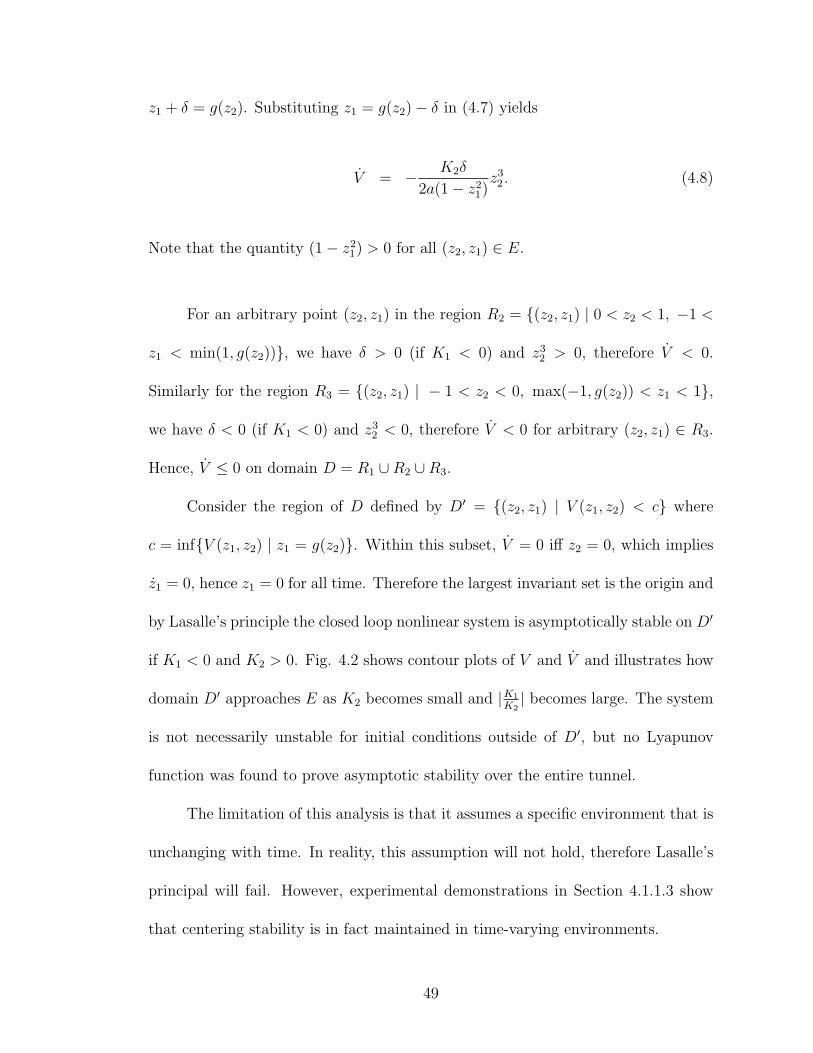
z1 + δ = g(z2). Substituting z1 = g(z2)− δ in (4.7) yields

V = − K2δ

2a(1− z21)

z32 . (4.8)

Note that the quantity (1− z21) > 0 for all (z2, z1) ∈ E.

For an arbitrary point (z2, z1) in the region R2 = (z2, z1) | 0 < z2 < 1, −1 <

z1 < min(1, g(z2)), we have δ > 0 (if K1 < 0) and z32 > 0, therefore V < 0.

Similarly for the region R3 = (z2, z1) | − 1 < z2 < 0, max(−1, g(z2)) < z1 < 1,

we have δ < 0 (if K1 < 0) and z32 < 0, therefore V < 0 for arbitrary (z2, z1) ∈ R3.

Hence, V ≤ 0 on domain D = R1 ∪R2 ∪R3.

Consider the region of D defined by D′ = (z2, z1) | V (z1, z2) < c where

c = infV (z1, z2) | z1 = g(z2). Within this subset, V = 0 iff z2 = 0, which implies

z1 = 0, hence z1 = 0 for all time. Therefore the largest invariant set is the origin and

by Lasalle’s principle the closed loop nonlinear system is asymptotically stable on D′

if K1 < 0 and K2 > 0. Fig. 4.2 shows contour plots of V and V and illustrates how

domain D′ approaches E as K2 becomes small and |K1

K2| becomes large. The system

is not necessarily unstable for initial conditions outside of D′, but no Lyapunov

function was found to prove asymptotic stability over the entire tunnel.

The limitation of this analysis is that it assumes a specific environment that is

unchanging with time. In reality, this assumption will not hold, therefore Lasalle’s

principal will fail. However, experimental demonstrations in Section 4.1.1.3 show

that centering stability is in fact maintained in time-varying environments.

49

−8

−8

−8

−8

−8

−8

−6

−6

−6

−6

−6

−6

−4

−4

−4

−4

−4

−4

−2

−2

−2

−2

−2

−2

−2

−2

−2

−2

0

0

0

0

2

2

4

4

6

6

8

8

−1 −0.5 0 0.5 1−1

−0.5

0

0.5

1A

B

_V > 0

R1 ±

−

z1z2( );

z2

_V > 0

z1

_V (z1; z2)

_V (z1; z2)

R2R3

g(z2)z1=

g(z2)z1=

0.5

0.5 0.5

0.5

0.50.5

0.5

1

1 1

1

1

1 1

1

1.51.5 1.5

1.51.5 1.5

22 2

2

22 2

2

2.5 2.5 2.5

2.5 2.5 2.5

33 3

3

33 3

3

3.5 3.5 3.5

3.5 3.5 3.5

4 4 4 4

4 4 4 4

−1 −0.5 0 0.5 1−1

−0.5

0

0.5

1

0.1

0.1

0.1

0.1

0.1

0.1

0.1

0.2

0.2

0.2

0.2

0.2

0.2

0.3

0.3

0.3

0.3

0.3

0.3

0.4

0.4

0.4

0.4

0.4

0.4

0.5

0.5

0.5

0.5

0.5

0.5

−1 −0.5 0 0.5 1−1

−0.5

0

0.5

1

−0.4

−0.4

−0.4

−0.4

−0.4

−0.4

−0.4

−0.4

−0.2

−0.2

−0.2

−0.2

−0.2

−0.2

−0.2

−0.2

−0.2

−0.2

−0.2

−0.2

00

00

−1 −0.5 0 0.5 1−1

−0.5

0

0.5

1

V (z1; z2)

V (z1; z2)

z2

z1

z2

z1

z2

z1

D’

D’

Figure 4.2: Contour plots of V and V and the regions D = R1 ∪ R2 ∪ R3 (whereV < 0) and D′ (for which asymptotic stability is guaranteed); (A) K1 = −24,K2 = 13 (gains used in 4.1.1.3), (B) K1 = −2.4, K2 = 0.13.

50

Wide-Field

Integration

X Vehicle

DynamicsOptic Flow

Computation

Gaussian

Blur

Camera &

Image

Grabbing

Spatial &

Temporal

Averaging

Optic Flow Measurement

Convert to

Motor

Commands

uref u x _Q

Figure 4.3: Information flow diagram for ground vehicle; x = (u, y, ψ), u = ur, uu,and uref = K3Nuref , 0.

4.1.1.3 Experimental Validation

To test the performance of the WFI-feedback concept on a real platform with

real-time sampling of optic flow, a wheeled vehicle was constructed. A modified Dr.

Robot X80 provided the chassis, wheel motors and motor control (Fig. 4.4A). A

Biostar computer with VIA motherboard and AMD CPU (1.3 GHz) interfaces with

the camera (FireFly MV, Point Grey Research), processes the imagery and sends

motor commands at 20 Hz over the serial port. A 360 field of view is obtained from

a parabolic mirror (0-360.com Panoramic Optic) installed above the robot, with

the FireWire camera pointing upward toward the mirror (Fig. 4.4B). The author

gratefully acknowledges Mike Chinn for design and assembly of the hardware. The

walls of the corridor (Fig. 4.5A and 4.6A) are composed of the imagery shown in

Fig. 4.4C.

Optic Flow Sensing and Computation

Fig. 4.3 illustrates the closed-loop process whereby the optic flow is measured

by the vehicle and used to control its motion. As the robot travels forward through

the tunnel, the camera is repeatedly accessed (240 × 240 resolution, 55 fps) by the

on-board C++ routine. To reduce high frequency spatial noise, the image extracted

51

A B

C

Figure 4.4: (A) Ground vehicle configuration, (B) Camera view with an examplering used for 1D optic flow extraction, and (C) Tunnel wall texture.

from the camera is first run through a low-pass spatial filter using an OpenCV

Gaussian blurring function.

For each frame, the embedded software captures a greyscale image. Using two

successive frames, optic flow is computed to determine the motion field around the

azimuth of the vehicle. An OpenCV implementation of the Lucas-Kanade pyramid

iterative algorithm [77] is used to compute the optic flow. This is a gradient-based

method using a maximum of 20 iterations at each pyramid level (3 levels used here),

and an initial guess of zero. The ‘pyramid’ scheme refers to the fact that optic

flow is first computed for lower resolution versions of the images (to increase the

maximum detectable shift), then this estimate is fed as an initial guess to the optic

flow computation for a higher resolution version, and so forth, until the maximum

resolution version is reached. Outlier solutions with high final cost function error,

or estimated shift components larger than a given search space size, are disregarded.

52

To compute the azimuthal optic flow efficiently, the movement of a set of 800

target pixels is tracked, all located in one of four concentric rings of pixels at fixed

radii from the mirror center (e.g., Fig. 4.4B). Each ring will capture a different

line of approximately constant height on the corridor wall. Four rings, rather than

one, are used to increase the number of measurements in the WFI thereby reducing

noise throughput to the actuators. The optic flow computation is 2-D, but only

the component of the shift tangent to the ring is used in the controller. By taking

the dot product of the shift vector with the ring tangent vector, an estimate is

obtained of the 1-D optic flow at 20 discrete angles around the vehicle. Each discrete

measurement is the average of 40 adjacent raw measurements across four rings, with

outlier measurements rejected. The optic flow for each frame combination can be

further smoothed by taking the block average over a time interval (assuming constant

optic flow during this period). The desired vehicle turn rate is computed via (4.3),

then the wheel speeds are calculated and sent to the motor controller board.

Results

The vehicle’s trajectory was tracked using a Vicon tracking system, which uses

8 cameras to triangulate the position of reflective markers attached to the vehicle.

It updates at 350 Hz and is accurate to less than 1 mm.

The centering response behavior is tested in a fixed-width 1.2 m corridor with

a 90 bend (Fig. 4.5A). The commanded forward speed is held constant for this

experiment at 0.43 m/s using local feedback from the motor speed controllers. Input

parameters include a turn saturation limit of 1 rad/s, and gains of K1 = −24,

K2 = 13. These gains were manually optimized to achieve rapid centering but with

53

0 100 200 300

−2

−1

0

0 100 200 300−1

0

1

A B C

D

0 2 4 6 8 10−0.2

−0.1

0

0.1

0.2

0.3

0 1 2

0

-1

-2

Time (s)

Fourier Coefficients

rad/s

x (m)

E F

G

Optic Flow

Angular Position (deg)

y (m)

tGt =

Ftt =

tGFt

t 0=

t 10=

°

_Q(°)

rad/s

rad/s

(F)

(G)

−2

−1

0

y (m)

−2

−1

0

y (m)

0 1 2

x (m)

0 1 2

x (m)

t 0=

t 10=

ya1ya2

Figure 4.5: Centering response in a 90 corridor for a fixed forward speed; (A)ground vehicle and wall textures, (B) trajectories (and mean) for 20 trials with acombined 0.25 m lateral and 45 orientation offset, (C) first ya1 and second ya2 cosineharmonics (WFI outputs), and means, for the 20 trials, (D) trajectories for differentinitial lateral offsets (0, 5, 10, 15 in.) and (E) orientation offsets (0, 30, 60, 80),(F) optic flow pattern Q(γ) measured at time t = tF and (G) at t = tG.

54

minimal overshoot and noise response. The turn saturation limit is imposed to avoid

undesirably large responses to noise in the ya1 and ya2 signals.

Examples of measured optic flow are shown in Fig. 4.5G, for a near-centered

path of travel, and Fig. 4.5F, where there is clear asymmetry in the signal due to the

lateral offset and a DC component due to the high turn rate of the vehicle. The optic

flow has surprisingly little noise, even in the presence of local areas of poor contrast

in the wall textures and in the front and back of the vehicle where there is no visual

texture. Additional irregularities in the sinusoid shape arise due to distortions in the

mapping of straight lines to concentric rings on the mirror, vibrations in the robot

chassis, reflections on the Plexiglas mirror mounting window, and camera noise.

The resulting variance in the trajectories in the figure shows that the approach can

robustly handle such non-idealities.

The initial lateral and orientation perturbations are evident in the ya1 and ya2

plots (Fig. 4.5C) and the controller is able to effectively regulate these to zero plus or

minus a finite tolerance due to measurement noise. The robustness of the method is

illustrated in Fig. 4.5B, which shows consistent trajectories (max standard deviation

2.0 cm) for 20 trials, and Fig. 4.5D-E, which partially validate the findings of 4.1.1.2

by demonstrating stability for large initial perturbations.

The clutter and centering responses were tested simultaneously using a converging-

diverging tunnel with a 0.76 m throat. Forward speed control is implemented by a

discrete-time controller which adds K3(Nuref − yb1) to the previous speed at every

control update. The maximum turn rate is scaled linearly downward from 1 rad/s

at 0.43 m/s (max speed) to 0.26 rad/s at 0.22 m/s (min speed) to avoid over-active

55

CA B

−1 0 1

0

1

2

3

4

5

0 1 2 3 40

0.1

0.2

0.3

0.4

0.5

0.6u

Distance Along Tunnel (m)x (m)

y (m)

(m/s)

t 0=

(rad/s)yb1

Figure 4.6: Clutter response for 20 trials; (A) converging-diverging tunnel environ-ment, (B) trajectories and mean, (C) forward speed u and first sine harmonic yb1

(WFI output) as a function of tunnel position for the 20 trials along with the mean.

control in the low bandwidth regime. This is also the reason for using lower gains

here (K1 = −2.4, K2 = 1.3 and K3 = 3.8), compared with the constant speed trials.

Fig. 4.6 shows that the centerline of the corridor is tracked well and the speed

is regulated to keep the first sine harmonic yb1 of optic flow roughly constant at

Nuref = 0.39. The orientation offset during recovery to the centerline causes a

deceptively low yb1 value due to nonlinearities in the yb1 expression (see [68]). When

the orientation offset is corrected, yb1 shoots up and the controller acts to control the

forward speed. The proportionality between velocity and corridor width is evident

in the latter half of the trajectory where the robot remains centered. These results

emulate the behavior seen in experiments with honeybees [26].

4.1.1.4 Optimal Weighting Functions for Planar Vehicles with a Non-

holonomic Sideslip Constraint

In [68], weighting functions that delivered static state estimates via a planar

WFI operation were found by trying Fourier harmonics and selecting appropriate

56

harmonics by inspection of the observation matrix C. Here, the method of Section

3.2.3 will be employed to obtain optimal weighting functions.

The infinite tunnel model is again assumed, and because parametric environ-

ment uncertainty (in the tunnel width) changes only the scaling of the 2-D environ-

ment, not the relative structure (as typically occurs in 3-D), the uncertainty in C

is neglected. The minimum variance estimator then results from filling the initial

weighting set Fy with all the elements of an infinite basis for L2[0, 2π], determining

C using the algebraic optic flow model, and applying (3.9) and (3.20). A close ap-

proximation is obtained by including Fourier harmonics in Fy up to ∼20th order,

but the exact optimum can also be obtained in a more efficient manner. If the optic

flow model is linearized about a desired pattern and the resulting state coefficients

are used as weighting functions Fy, then the Fisher information is maximized with

respect to the model and (3.9) and (3.20) deliver the optimum (minimum variance)

state extraction weighting functions. In more detail:

1. Linearize Q (sideslip neglected) about the nominal trajectory:

Qlin =

y v0 sin 2γa2 + ψ v0 sin 2γ

2a+ u sin 2γ

a− ψ, 0 ≤ γ + ψ < π

y v0 sin 2γa2 − ψ v0 sin 2γ

2a− u sin 2γ

a− ψ, π ≤ γ + ψ < 2π

. (4.9)

2. Set Fyi= ∂Qlin

∂xiand perform WFI of Qlin. Note that this gives the same result

as using the non-linear Q and linearizing the WFI outputs (see Section A.1).

yi =

∫ 2π

0

Qlin∂Qlin

∂xi

dγ. (4.10)

57

3. Collate results into an observation matrix C:

y1

y2

y3

y4

=

3πv20

4a4 0 0 −πv0

a2

0πv2

0

4a2 0 0

0 0 3π4a2 0

−πv0

a2 0 0 2π

y

ψ

u

ψ

. (4.11)

4. Since m = n, the system is exactly determined and the optimum weighting

functions for static state extraction are defined by the vector of functions

Fx = C−1Fy. The function ∂Qlin

∂xirepresents a perturbation pattern that is

imposed on the nominal flow pattern when state xi becomes non-zero. Since

these are not necessarily orthogonal, the inversion step (3.20) is required to

isolate the effect of each state.

Fy = −2a2

πv0

cos 2γ (4.12)

Fψ =

2aπv0

sin 2γ, 0 ≤ γ < π

− 2aπv0

sin 2γ, π ≤ γ < 2π

Fu =

4a3π

sin2γ, 0 ≤ γ < π

− 4a3π

sin2γ, π ≤ γ < 2π

Fψ = − 1

2π(1 + 2 cos 2γ) .

The choice of Fy as the Jacobian of the optic flow model results in the same Fisher

information as an Fy that fully spans L2[0, 2π] because the span of Fy here is iden-

58

tical to the span of the optic flow model. Therefore, the observation set delivers as

much information as possible about the model. Any additional observations (weight-

ing functions) are redundant and therefore do not increase the Fisher information.

Compared with the Fourier set Fy = Fa0 , Fa1 , Fa2 , Fb1 employed in past WFI

studies [65, 67], the optimum functions in (4.12) will provide state estimates with a

modest 3% reduction in variance; hence the Fourier choice was close to optimum.

4.1.2 Quadrotor using Ring-constrained WFI

This section summarizes the outcome of a WFI experiment using a micro

quadrotor (Fig. 4.7), the short comings of which provide motivation for the 2-D

WFI techniques described in Section 4.2. To demonstrate WFI-based navigation

on a 6-DOF platform, the 1-D sensing methodology of 4.1.1 was utilized, along

with sonar-based altitude regulation to maintain near-planar flight. The quadrotor

vehicle was fully autonomous, with all vision hardware onboard. A panoramic mirror

and camera were used for y and ψ estimation and a downward pointing Centeye

sensor provided estimates of u and v, after subtracting off rotation components q

and p using gyro data. The author gratefully acknowledges Joe Conroy and Greg

Gremillion for the hardware design, assembly and test, and Badri Ranganathan for

integration of my floating point WFI software on to the fixed point processor. The

reader is referred to [75] for vehicle details and experimental results.

The experiment successfully demonstrated simple corridor navigation, but sig-

nificant trajectory variance occurred due to errors in the estimation of forward speed

and sideslip from the downward-pointing optic flow sensor, which exhibited extreme

59

Camera

Parabolic Mirror

Avionics

Sonar Sensor Optic Flow Sensor

Camera

Parabolic Mirror

Avionics

Sonar Sensor Optic Flow Sensor

Figure 4.7: Schematic diagram of quadrotor components.

texture dependence. Differing frequency response characteristics between the Cent-

eye sensor and the gyros further compounded u and v measurement anomalies.

This motivates the need for spherical WFI of optic flow over a larger field of view,

with optimal weighting patterns. Such a scheme should deliver more reliable state

estimates, without the need to fuse-in gyro data.

The derivation of the optimal WFI weighting functions (4.1.1.4) used in this

experiment required that sideslip be neglected to maintain a full rank C matrix.

When optic flow is measured only in an equatorial ring, the perturbation pattern

induced by an orientation offset ψ is exactly opposite to that induced by sideslip v,

hence these quantities cannot be distinguished from one another (e.g., Eq. (5.1)).

The differing signs also imply that stabilizing feedback of ψ (obtained from equato-

rial ring WFI) will destabilize the v dynamics. Although this is countered somewhat

by sideslip regulation from the Centeye sensor, the limited bandwidth of this feed-

back loop prevent the use of large feedback gains on the ψ signal. This constrains

60

Roll Ring

R

R

R

Pitch Ring

Yaw Ring

P

Y

r (°; ¯)

r

TrS1

L

Figure 4.8: Fixed-wing UAV with ring-constrained optic flow sensing.

the performance of the system, preventing it from navigating the tight bends demon-

strated in 4.1.1.3. Spherical WFI over a wider field of view would allow the coupled

quantities to be separated (as is demonstrated in 4.2.2), thus removing the gain

limitation.

4.2 2-D WFI Demonstrations

4.2.1 Fixed-Wing UAV using Ring-constrained WFI

In this section, the gap between planar 1-D WFI and full spherical 2-D WFI

is bridged by considering 2-D optic flow measured in three orthogonal planes (Fig.

4.8). This allows extraction of all relevant navigational and motion states for a

6-DOF vehicle with vision sensing required over a relatively small percentage of the

sphere. This estimation methodology will be applied to the task of fixed-wing UAV

navigation in a simplified urban environment.

61

4.2.1.1 WFI-Based Controller

With the optic flow measurements constrained to three orthogonal planes (yaw,

pitch, roll), see (2.4), the general WFI operation (2.17) simplifies to

yki,j(x) = 〈Qk

j , Fi〉 =

∫ 2π

0

Qkj (β,x) Fi(β) dβ (for R and P planes),

yYi,j(x) = 〈QY

j , Fi〉 =

∫ 2π

0

QYj (γ,x) Fi(γ) dγ (for Y plane), (4.13)

where i is the output number, j is the is the plane of interest and k is the direction

of flow under scrutiny - either the β or γ direction.

In each plane, Fourier harmonics up to 2nd order were used for the initial

weighting function set Fy, and the flat surface world (2.10) was assumed for the

optic flow model, with no roof (hU → ∞) and no front/rear surfaces (g → ∞); see

Table 2.1 for the planar distance functions. The resulting C matrices for the limiting

cases of the parameterized environment are presented in Table 4.1, and are cropped

to display just n outputs, considered to provide the most consistent measurements

of each state given the environment uncertainty. Note that pitch ring optic flow

provides the most reliable measurements in this respect because all the uncertainty

is in the lateral obstacle environment and not the longitudinal.

To account for the uncertainty in C, an inversion matrix C† was manually de-

signed; presented in Table 4.3 (2nd column) in condensed form. In its construction,

a harmonic was used to decouple another harmonic (that encoded multiple states)

only if the states encoded by the first harmonic were consistent across the environ-

62

Table 4.1: Linearized 3-Ring optic flow decomposition for baseline environments

WFI Output Floor Right-side Wall with Floor Tunnel with Floor

yβb1,R

23πh

w 13πf1

v + 2hf1+2h2+af1+a2

3πhaf1w 2(a2+2hf1+2h2)

3πhaf1w

yγb2,R

4uref

3πhφ − 2

3πf1u− f2φ− 2huref

3πf21 f1

z − 2auref

3πf21 f1

y −f3φ− 4urefa3πf2

1 f1y

yβa1,P −4uref

3πh2 z − 43πh

u −4uref

3πh2 z − 43πh

u −4uref

3πh2 z − 43πh

u

yβb1,P

2uref

3πhθ + 2

3πhw 2uref

3πhθ + 2

3πhw 2uref

3πhθ + 2

3πhw

yγa0,P −

√2

πhv −

√2

πhv −

√2

πhv

yγa1,P − 1

2hv + p − 1

2hv + p − 1

2hv + p

yγb1,P −r −r −r

yβa1,Y −q −q −q

yγa1,Y 0 2uref

3πaψ − 2

3πav 4uref

3πaψ − 4

3πav

yγa2,Y 0 −uref

4a2 y − 14a

u −uref

2a2 y

yγb1,Y 0 4uref

3πa2 y + 43πa

u 83πa

u

note: f1 =√

h2 + a2 f2 = 2(h2+hf1−af1−a2)uref

3πhaf1f3 = 4(h2+hf1−a2)uref

3πahf1

ment extremes and the decoupling did not depend on knowledge of environment

parameter a. For these reasons, it was assumed that independent measurements of

u and φ are available. Note that this assumption could be avoided through use of

the more rigorous methods of Section 3.2, which will be demonstrated in 4.2.2.

The dynamics of the vehicle (4.14) are taken from a low-speed fixed wing

UAV; the 4.5 kg Gap 65 [78] with 1.8 m wingspan. Aerodynamic and gravity forces

are linearized about the steady, wings-level flight condition with a forward speed of

u0=12.5 m/s. For simulation, the linearized forces are implemented in a non-linear

63

dynamics and kinematics engine.

u = −gθ +Xu

m(u− u0) +

Xw

mw +

1

mδT − qw + rv

v = gφ +Yv

mv +

Yp

mp +

Yr

mr +

Yδa

mδa +

Yδr

mδr − ru + pw

w =Zu

m(u− u0) +

Zw

mw +

Zq

mq +

Zδe

mδe − pv + qu

p =

(Lv

Ixx

+Nv

f4

)v +

(Lp

Ixx

+Np

f4

)p +

(Lr

Ixx

+Nr

f4

)r +

(Lδa

Ixx

+Nδa

f4

)δa

+

(Lδr

Ixx

+Nδr

f4

)δr + pnl

q =Mw

Iyy

w +Mq

Iyy

q +Mδe

Iyy

δe + qnl (4.14)

r =

(Nv

Izz

+Lv

f4

)v +

(Np

Izz

+Lp

f4

)p +

(Nr

Izz

+Lr

f4

)r +

(Nδa

Izz

+Lδa

f4

)δa

+

(Nδr

Izz

+Lδr

f4

)δr + rnl

f4 =IxxIzz − I2

xz

Ixz

pnl

qnl

rnl

= [I]−1

p

q

r

× [I]

p

q

r

.

Actuator saturation limits are: |δr| ≤ 0.5 rad, |δT | ≤ ±5.3 N, |δe| ≤ 0.35 rad and

|δa| ≤ 0.35 rad. Characteristic stability quantities are defined in Table 4.2 with SI

units and all symbols having their usual meaning.

The control strategy consists of an inner tracking loop u = K(x−xref) and an

outer trajectory generation loop for lateral steering φref = Kφref ,y(y−yref)+Kφref ,ψψ,

turn coordination and altitude measurement correction at high bank. The dynamic

reference trajectory is presented in Table 4.3. Environment parameters are set to

64

Table 4.2: Fixed-wing UAV stability characteristics

Physical Parameters Longitudinal Derivatives Lateral Derivatives

m = 4.50 Xu = −0.84 Yv = −3.87g = 9.81 Xw = 0.20 Yp = 0.51

Ixx = 0.16 Zu = −0.94 Yr = 1.39Iyy = 0.60 Zw = −22.66 Yδa = −1.16Izz = 0.66 Zq = −7.80 Yδr = 7.96Ixz = 0.01 Zδe = −29.61 Lv = −0.40

Mw = −0.94 Lp = −2.99Mq = −3.26 Lr = 0.66

Mδe = −21.89 Lδa = 26.90Lδr = 0.52Nv = 1.24

Np = −0.32Nr = −1.15Nδa = 1.76

Nδr = −6.77

h = 10 m and a = 8. The latter is a rough pre-flight estimate of the tunnel half-width

or lateral distance to an obstacle, which acts only to scale the y and ψ navigational

gains.

The elevator and aileron control laws can therefore be written as

δe = Kδe,u(u− uref) + Kδe,w

(3πh

2yβ

b1,R

)+ Kδe,q(−yβ

a1,Y − qref) + Kδe,θ

(3πh

2uref

yβb1,P

)

+Kδe,z

(− h

4uref

(3πhyβa1,P + 4u)− zref

)(4.15)

δa = Kδa,v

(− πh√

2yγ

a0,P

)+ Kδa,p

(yγ

a1,P −π√

2

4yγ

a0,P

)+ Kδa,r(−yγ

b1,P − rref)

+Kδa,φ(φ− φref).

The feedback for the engine thrust and rudder control are the same as above,

65

Table 4.3: Inversion of Fourier outputs (to obtain static state estimates) and desiredtrajectory

State Estimation Law Desired (Reference) State Value

y − 2a2

urefyγ

a2,Y 0

z − h4uref

(3πhyβa1,P + 4u) h(cos φ− 1)

φ φ Kφref ,y

(− 2a2

urefyγ

a2,Y − yref

)+ Kφref ,ψ

(3πa4uref

yγa1,Y − ψref

)

θ 3πh2uref

yβb1,P 0

ψ 3πa4uref

yγa1,Y 0

u u u0

v − πh√2yγ

a0,P 0

w 3πh2

yβb1,R 0

p yγa1,P − π

√2

4yγ

a0,P 0

q −yβa1,Y

9.81u

sin φ tan φ

r −yγb1,P

9.81u

sin φ

with subscripts adjusted. State-feedback LQR is employed to obtain a set of opti-

mal feedback gains. After iteration with the simulator, the LQR control penalty

matrix was set to Ju =diag(300, 10−2, 60, 180) and the state penalty matrix to

Jx =diag(10−20, 20, 120, 1, 10−20, 2, 25, 1, 1, 180, 60). Outer-loop gains were deter-

mined via manual tuning. Table 4.4 lists the final gains.

Table 4.4: Fixed-wing UAV feedback gains

Elevator Thrust Aileron Rudder Roll Angle

Kδe,z = −0.26 KδT ,z = 5.07 Kδa,φ = −1.74 Kδr,φ = −0.27 Kφref ,y = −0.10Kδe,θ = 2.94 KδT ,θ = −16.03 Kδa,v = −0.19 Kδr,v = −0.18 Kφref ,ψ = −1.80Kδe,u = 0.00 KδT ,u = −13.46 Kδa,p = −0.12 Kδr,p = −0.03

Kδe,w = −0.08 KδT ,w = 1.97 Kδa,r = 0.28 Kδr,r = 0.64Kδe,q = 0.71 KδT ,q = −0.23

66

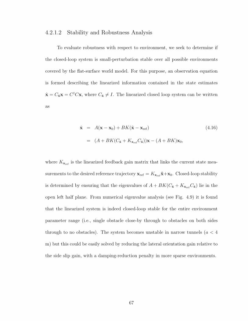
4.2.1.2 Stability and Robustness Analysis

To evaluate robustness with respect to environment, we seek to determine if

the closed-loop system is small-perturbation stable over all possible environments

covered by the flat-surface world model. For this purpose, an observation equation

is formed describing the linearized information contained in the state estimates

x = Cxx = C†Cx, where Cx 6= I. The linearized closed loop system can be written

as

x = A(x− x0) + BK(x− xref) (4.16)

= (A + BK(Cx + KxrefCx))x− (A + BK)x0,

where Kxrefis the linearized feedback gain matrix that links the current state mea-

surements to the desired reference trajectory xref = Kxrefx+x0. Closed-loop stability

is determined by ensuring that the eigenvalues of A + BK(Cx + KxrefCx) lie in the

open left half plane. From numerical eigenvalue analysis (see Fig. 4.9) it is found

that the linearized system is indeed closed-loop stable for the entire environment

parameter range (i.e., single obstacle close-by through to obstacles on both sides

through to no obstacles). The system becomes unstable in narrow tunnels (a < 4

m) but this could be easily solved by reducing the lateral orientation gain relative to

the side slip gain, with a damping-reduction penalty in more sparse environments.

67

Right-Side Wall with Floor Tunnel with Floor

Figure 4.9: Root locus diagrams for range of environments and obstacle spacings.Closed-loop eigenvalues computed for a up to 1000 m (∼ ∞) in steps of 0.5 m. A’no obstacles’ environment is obtained when a →∞.

4.2.1.3 Simulation

The WFI-based state estimates provide adequate information to stabilize and

navigate with the linearized vehicle model, but we must verify performance in the

face of measurement noise, nonlinearities (Eq. (4.14)) and differences between the

true environment and its mathematical approximation. For this purpose, a virtual

UAV was simulated in two different environments using an in-house simulation en-

gine (AVLSim). Environment A (Fig. 4.10A) simulates the ‘right side-wall with

floor’ scenario, whilst environment B (Fig. 4.10B) simulates a ‘tunnel with floor’

world and has the additional challenges of a 20 terrain ramp and a 30 bend in the

16 m wide tunnel.

Optic Flow Sensing and Computation

AVLSim provides visualization capabilities as well as the ability to compute

optic flow from simulated cameras. The virtual UAV is installed with six cameras,

68

A B

Figure 4.10: 3-D simulation environments; (A) single wall, (B) tunnel with 20 rampand 30 bend.

each with a 90 × 90 field-of-view and a resolution of 128 × 128 pixels. The cameras

cover the six sides of a cube such that the three orthogonal measurement rings are

fully imaged. The imagery is first passed through a Gaussian blurring function to

reduce high frequency spatial noise. Images are combined to form a 360 panorama

for each ring, and optic flow is computed with a resolution-iterative implementation

of the Lucas-Kanade algorithm at 30 fps for 1600 image points per panorama. The

environment surfaces and sky are textured with imagery of sufficient visual contrast

so that optic flow can be computed.

The optic flow measurement nodes are located in one of four rows, around the

mid-line of the panoramic image, with a vertical separation of 4 pixels (i.e., max

out-of-plane angle = 5). The measurement points (Fig. 4.11) have equal azimuthal

spacing and are assigned to pixel coordinates by projecting points on a circle to

a flat camera surface. Shift estimate magnitude is also corrected for flat-camera

distortion. Measurements are averaged horizontally to converge 400 data points to

69

−180 −90 0 90 180

30

60

90

120

150

azimuth (deg)

ele

va

tio

n (

de

g)

Pitch RingPitch Ring Roll RingRoll Ring

Yaw

Ring

Figure 4.11: Optic flow sampling regions. Cameras form panoramas in 3 orthogonalplanes, but optic flow is only measured in the mid-line regions of the panoramas.

just 20, then averaged vertically among the four rows of measurements. In both

these steps outlier measurements with high final cost function or infeasibly large

shift estimates are ignored in order to improve the signal to noise ratio. In the

wide-field integration, the six spatial optic flow functions (for flow tangential and

normal to each ring) are decomposed into their Fourier harmonics up to 2nd order.

These are low-pass filtered in the temporal domain with a cut-off frequency of 30

rad/s to further reduce noise. The filtered values are then scaled and combined

in the manner according to (4.15) to obtain the UAV actuator inputs. To avoid

the ground being perceived as a lateral obstacle, the bank angle is constrained by

shutting off lateral actuators when |φ| > 30. The simulation process is illustrated

in Fig. 4.12.

70

Form Panora-

mas for each

Plane (Yaw,

Pitch, Roll)

Gaussian

Image Blur

Lucas-Kanade

Optic Flow (400

x 4 Datapoints

per Plane)

Spatial Averag-

ing & Outlier

Rejection (400

x 4 → 20)

Wide-Field

Integration

Scale &

Combine

Outputs /

Measurements

u yx UAV

Kinematics

& Dynamics

Visual

Environment

Compute

Reference

Trajectory

_Q

xref

Compute

Controls

Wide Field Integration & Control

Optic Flow Measurement

Low Pass

Temporal

Filter h _Q;F i

Grab Images

from 6

Cameras

¡K(x¡ xref)

x

Figure 4.12: Ring-constrained WFI simulation process diagram.

Results

To demonstrate robustness with respect to initial conditions, several cases

were simulated in each environment. Fig. 4.13 shows that the aircraft is able to

successfully avoid the obstacles while maintaining a target height of ∼10 m above

the ground in both environments. The initial lateral and vertical offsets in the tunnel

do not affect the downrange trajectory. However, the different orientation offsets

in the single-wall environment (Fig. 4.13A) lead to different final trajectories due

to the finite length of the wall. When the aircraft flies beyond the wall there is a

tendency to turn back toward the wall edge to balance obstacle orientation.

The plots of motion states (Fig. 4.14) for the Fig. 4.13B tunnel case indicate

impressive accuracy in the measurement of side slip and angular rates. This is due

to the fact that these quantities do not scale with a, unlike the w measurement,

which appears poorly scaled because of its sensitivity to the presence of lateral

obstacles. A pure scaling discrepancy is roughly equivalent to scaling the applicable

71

A B

i)

ii)

−30

0

0 50 100 150 200

x (m)

y (m)

0 50 100 150 200

−100

10

x (m)

z (m)

−20

−10

0

10

20

30

0 20 40 60 80

x (m)

y (m)

C D

0 10 20 30 40 50

−15

−10

−5

0

5

10

x (m)

z (m)

−10

0

10

0 10 20 30 40 50x (m)

y (m)

Figure 4.13: Simulation results - trajectories. (A) Single wall (initial ψ =0, 15, 30, 45): plan view; (B) tunnel with 20 ramp and 30 bend (initialy = 2, z = 2 m,ψ = 15): i) side view, ii) plan view. (C) tunnel (initialy = −4,−2, 2, 4 m): plan view; (D) tunnel (initial z = −5,−2.5, 2.5, 5 m): sideview.

0 5 10 15 20

−10

0

10

(m/s)

0 5 10 15 20

−10

0

10

(m/s)

0 5 10 15 20

−10

0

10

time (s)

(m/s)

0 5 10 15 20

−2

0

2

(rad/s)

0 5 10 15 20

−2

0

2

(rad/s)

measured

true

target

0 5 10 15 20

−2

0

2

time (s)

(rad/s)

uv

w

pq

r

Figure 4.14: Simulation results for tunnel environment (initial y = 2, z = 2 m,ψ =15): speeds, rates and optic-flow-extracted measurements.

72

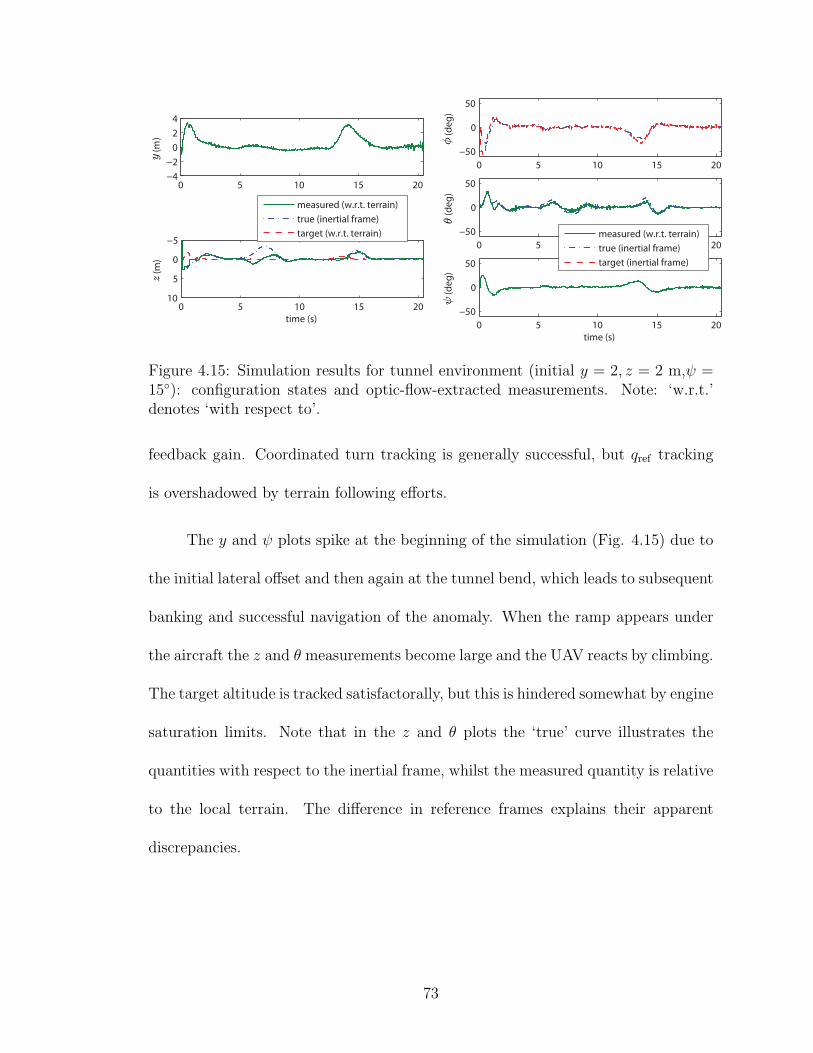
0 5 10 15 20−4

−2

0

2

4

(m)

0 5 10 15 20

−5

0

5

10

time (s)

(m)

0 5 10 15 20

−50

0

50

(deg)

0 5 10 15 20

−50

0

50

(deg)

0 5 10 15 20

−50

0

50

time (s)

(deg)

measured (w.r.t. terrain)

true (inertial frame)

target (inertial frame)

Áµ

Ã

yz

measured (w.r.t. terrain)

true (inertial frame)

target (w.r.t. terrain)

Figure 4.15: Simulation results for tunnel environment (initial y = 2, z = 2 m,ψ =15): configuration states and optic-flow-extracted measurements. Note: ‘w.r.t.’denotes ‘with respect to’.

feedback gain. Coordinated turn tracking is generally successful, but qref tracking

is overshadowed by terrain following efforts.

The y and ψ plots spike at the beginning of the simulation (Fig. 4.15) due to

the initial lateral offset and then again at the tunnel bend, which leads to subsequent

banking and successful navigation of the anomaly. When the ramp appears under

the aircraft the z and θ measurements become large and the UAV reacts by climbing.

The target altitude is tracked satisfactorally, but this is hindered somewhat by engine

saturation limits. Note that in the z and θ plots the ‘true’ curve illustrates the

quantities with respect to the inertial frame, whilst the measured quantity is relative

to the local terrain. The difference in reference frames explains their apparent

discrepancies.

73

4.2.2 Micro Helicopter using Spherical WFI

In this section, the rigorous methods developed in Chapter 3 are applied to

design weighting patterns that converge optic flow measured over the full sphere

to actuator commands that stabilize a micro helicopter and permit navigation of a

cluttered environment.

4.2.2.1 WFI-Based Controller

The vehicle selected for simulation is the 390 g E-sky Hobby Helicopter, with a

50.5 cm main rotor diameter and a 14.5 cm tail rotor. A linearized flight dynamics

model was obtained in a prior study [79] via system identification with the US

Army’s CIFER software package. The kinematics and dynamics (4.17) are linearized

about the forward flight condition, with uref=1 m/s. For simulation, the full non-

74

linear kinematic equations are used.

u = −gθ + Xuu

v = gφ + Yvv − urefr

w = Zww + ZΩmrΩmr + urefq

p = Lvv + Lξξ

q = Muu + Mχχ (4.17)

r = Nrr + NΛyawΛyaw

ξ = −p− 1

τf

ξ +ξχ

τf

χ +ξlat

τf

Λlat +ξlon

τf

Λlon

χ = −q +χξ

τf

ξ − 1

τf

χ +χlat

τf

Λlat +χlon

τf

Λlon

Ωmr = TΩmrΩmr + TΛtΛt.

The actuator saturation limits are: |Λlat| ≤ 1, |Λlon| ≤ 1, |Λt| ≤ 0.5 and |Λyaw| ≤ 1.

Characteristic stability quantities are defined in Table 4.5 with SI units.

Table 4.5: Micro helicopter stability characteristics

Xu = −0.5214 τf = 0.15Yv = −0.4799 ξχ = 1.55Zw = −0.6802 ξlat = 0.245ZΩmr = 0.170 ξlon = 0.043Lv = −8.246 χξ = −2.82Lξ = 1273 χlat = 0.044Mu = 3.599 χlon = −0.202Mχ = 341.6 TΩmr = −6.182

Nr = −0.8786 TΛt = 1449NΛy = 39.06 g = 9.81

75

The feedback control objective is to regulate the relative state estimates pro-

vided by WFI to specified reference values, thereby generating stable obstacle avoid-

ance and terrain following behaviors. The proposed methodology assumes that an

altitude measurement z is available for feedback, along with the actuator states

ξ, χ, Ωmr. The independent altitude measurement is required to remove target

altitude dependence on obstacle distribution in the environment (see Section 7.5).

The estimates for the remaining 10 relative states are generated using the optimal

weighting functions from (3.20),

xi = 〈Q,Fxi〉+ C†

i,M+1z, (4.18)

where M + 1 is the column of C† corresponding to the independent attitude mea-

surement z. The initial weighting pattern set Fy is chosen to be spherical harmonics

up to 10th degree. Construction of the C matrix can only be done numerically given

the complexity of the distance function (2.10) (flat surface world assumed, without

front and rear surfaces, as in (3.8)), and it is too large to present here. With the

angular spacing of measurement nodes set to 9 for real-time implementation, the

weighted-least squares inversion (3.9) results in the state extraction functions pre-

sented in Fig. 4.16. Note that the u-estimator pattern extracts forward speed from

the ground-induced optic flow rather than from lateral obstacles. This is a direct

consequence including the term RδC in the design of C†, which penalizes the uncer-

tain spacing of lateral objects compared with the relatively well known proximity of

the ground.

76

−180 −90 0 90 1800

45

90

135

180

Optimum Extraction Pattern

azimuth (deg)

ele

va

tio

n (

de

g)

−180 −90 0 90 1800

45

90

135

180

Optimum Extraction Pattern

azimuth (deg)

ele

va

tio

n (

de

g)

−180 −90 0 90 1800

45

90

135

180

Optimum Extraction Pattern

azimuth (deg)

ele

va

tio

n (

de

g)

q

−180 −90 0 90 1800

45

90

135

180

Optimum Extraction Pattern

azimuth (deg)

ele

va

tio

n (

de

g)

−180 −90 0 90 1800

45

90

135

180

Optimum Extraction Pattern

azimuth (deg)

ele

va

tio

n (

de

g)

w

−180 −90 0 90 1800

45

90

135

180

Optimum Extraction Pattern

azimuth (deg)

ele

va

tio

n (

de

g)

v

−180 −90 0 90 1800

45

90

135

180

Optimum Extraction Pattern

azimuth (deg)

ele

va

tio

n (

de

g)

u

−180 −90 0 90 1800

45

90

135

180

Optimum Extraction Pattern

azimuth (deg)

ele

va

tio

n (

de

g)

Ã

−180 −90 0 90 1800

45

90

135

180

Optimum Extraction Pattern

azimuth (deg)

ele

va

tio

n (

de

g)

−180 −90 0 90 1800

45

90

135

180

Optimum Extraction Pattern

azimuth (deg)

ele

va

tio

n (

de

g)

y Á

µ

p r

Figure 4.16: Optimum weighting patterns to recover environment-scaled states fromoptic flow field.

77

It has been assumed that the vehicle can measure optic flow over the entire

spherical viewing arena, but this may create hardware design complications and

possible optic flow computation issues if the sky is uniformly blue or overcast. A

rotating vehicle will not induce a perceptable optic field with a zero-contrast back-

ground, thus all WFI-based relative states will be distorted, leading to potential

instability. It is therefore beneficial for robustness to measure optic flow below the

horizon only - where the existence of suitable image contrast is more probable. The

measurement domain can theoretically be arbitrarily small and still permit relative

state estimates via WFI, however Fisher information theory shows that the esti-

mates will become less robust to noise as the field of view decreases. Using (3.8)

and (3.15), it can be shown that the noise throughput (3.18) roughly triples by re-

stricting the field-of-view to below the horizon only. This is deemed an acceptable

price for the ability to operate in conditions where the sky has no visual contrast.

The optimum weighting patterns with a lower hemisphere measurement grid are

presented in Fig. 4.17. The default design will still use the full spherical weightings,

but a performance comparison (Fig. 4.24C-D) will be made with the alternative

half-sphere configuration.

The desired reference for the state vector x = (y, z, φ, θ, ψ, u, v, w, p, q, r, ξ, χ, Ωmr),

which accounts for the pitch and rotor speed variation from hover required to reach

1 m/s, is taken as

xref = (0, Kz,θ(θ − θ), 0,−0.05, 0, 1.00, 0,−0.05, 0, 0, 0, 0, 0, 0.21). (4.19)

78

−180 −90 0 90 1800

45

90

135

180

Optimum Extraction Pattern

azimuth (deg)

ele

va

tio

n (

de

g)

−180 −90 0 90 1800

45

90

135

180

Optimum Extraction Pattern

azimuth (deg)

ele

va

tio

n (

de

g)

−180 −90 0 90 1800

45

90

135

180

Optimum Extraction Pattern

azimuth (deg)

ele

va

tio

n (

de

g)

−180 −90 0 90 1800

45

90

135

180

Optimum Extraction Pattern

azimuth (deg)

ele

va

tio

n (

de

g)

−180 −90 0 90 1800

45

90

135

180

Optimum Extraction Pattern

azimuth (deg)

ele

va

tio

n (

de

g)

−180 −90 0 90 1800

45

90

135

180

Optimum Extraction Pattern

azimuth (deg)

ele

va

tio

n (

de

g)

−180 −90 0 90 1800

45

90

135

180

Optimum Extraction Pattern

azimuth (deg)

ele

va

tio

n (

de

g)

−180 −90 0 90 1800

45

90

135

180

Optimum Extraction Pattern

azimuth (deg)

ele

va

tio

n (

de

g)

−180 −90 0 90 1800

45

90

135

180

Optimum Extraction Pattern

azimuth (deg)

ele

va

tio

n (

de

g)

−180 −90 0 90 1800

45

90

135

180

Optimum Extraction Pattern

azimuth (deg)

ele

va

tio

n (

de

g)

q

wv

uÃ

y Á

µ

p r

Figure 4.17: Optimum weighting patterns to recover environment-scaled states fromoptic flow field, restricted to lower hemisphere measurements.

79

Note the target altitude offset zref = Kz,θ(θ− θ) is a function of the pitch angle mea-

surement relative to the gravity vector θ (assumed to be provided by an additional

sensor) and the WFI estimate θ from (4.18), which provides an indication of upcom-

ing terrain. This form of the reference is chosen in order to avoid unacceptable speed

loss during climbs over steep terrain. To prevent excessive or unnecessary vertical

velocities, zref is intentionally restricted to be zero except when in the range (-1,0).

Furthermore, the pitch angle estimate θ is subtracted from the WFI-based estimate

θ to preclude superfluous climb commands arising from the nominal specified value

of θ = −0.05. It is important to note that different behaviors can be rapidly realized

during flight by adjusting the target state (4.19) - which essentially specifies desired

optic flow asymmetry. Setting a non-zero yref , for example, will cause the vehicle to

track a non-centered path or, in the extreme, hug a wall.

Assuming a linear tracking controller, the structure of the feedback law can

be written as:

uk =∑

i

Kk,xi

(〈Q,Fxi

〉+ C†i,M+1z − xi,ref

)+

∑j

Kk,xj(xj − xj,ref ), (4.20)

where k = Λlat, Λlon, Λt, Λyaw denotes the actuator input, i = y, φ, ψ, u, v, w, p, q, r

is the set of WFI-based state measurements and j = z, θ, ξ, χ, Ωmr is the set of

states measured with alternate sensors. LQR is employed to obtain a set of optimal

feedback gains. After iteration with the simulator, the LQR state penalty matrix

was set to Jx =diag(25, 1, 1, 1, 5, 100, 20, 5, 1, 1, 1, 10−15, 10−15, 10−15) and the control

penalty matrix to Ju =diag(1, 1, 1, 1). Table 4.6 lists the final gains.

80

Table 4.6: Micro helicopter feedback gains

Cyclic Lat. Cyclic Lon. Main Rotor Tail Reference

KΛlat,y = −4.70 KΛlon,y = −0.12 KΛt,y = 0.01 KΛyaw,y = −1.70 Kz,θ = 3.50KΛlat,z = 0.00 KΛlon,z = 0.01 KΛt,z = 1.00 KΛyaw,z = 0.00

KΛlat,φ = −11.05 KΛlon,φ = −0.17 KΛt,φ = 0.03 KΛyaw,φ = 1.78KΛlat,θ = −0.73 KΛlon,θ = 19.02 KΛt,θ = −0.63 KΛyaw,θ = 0.03KΛlat,ψ = −3.42 KΛlon,ψ = −0.07 KΛt,ψ = 0.01 KΛyaw,ψ = −2.60KΛlat,u = 0.22 KΛlon,u = −8.70 KΛt,u = 0.18 KΛyaw,u = −0.01

KΛlat,v = −4.35 KΛlon,v = −0.17 KΛt,v = 0.01 KΛyaw,v = 2.01KΛlat,w = 0.00 KΛlon,w = 0.06 KΛt,w = 2.20 KΛyaw,w = 0.00KΛlat,p = −0.81 KΛlon,p = 0.13 KΛt,p = 0.00 KΛyaw,p = 0.03KΛlat,q = 0.05 KΛlon,q = 1.32 KΛt,q = 0.07 KΛyaw,q = 0.00KΛlat,r = 0.03 KΛlon,r = 0.00 KΛt,r = 0.00 KΛyaw,r = −1.09

KΛlat,ξ = −29.70 KΛlon,ξ = −4.35 KΛt,ξ = −0.10 KΛyaw,ξ = 0.64KΛlat,χ = −5.49 KΛlon,χ = 20.43 KΛt,χ = 0.48 KΛyaw,χ = 0.09KΛlat,Ωmr = 0.00 KΛlon,Ωmr = 0.00 KΛt,Ωmr = −0.02 KΛyaw,Ωmr = 0.00

As described in Chapter 3, the control law can be rewritten in a more compu-

tationally efficient form that requires only one WFI operation per actuator;

uk = 〈Q,Fuk〉+

∑i

Kk,xi

(C†

i,M+1z − xi,ref

)+

∑j

Kk,xj(xj − xj,ref ), (4.21)

where the sensor-to-actuator mapping patterns Fukare defined in (3.5) and pre-

sented in Fig. 4.18.

4.2.2.2 Stability and Robustness Analysis

The robust stability analysis of Section 4.2.1.2 is applied to the micro helicopter

with full-sphere WFI. The observation equation describing the linearized information

81

−180 −90 0 90 1800

45

90

135

180

azimuth (deg)

ele

va

tio

n (

de

g)

Delta Thrust Input t

Flow Weighting Pattern

−180 −90 0 90 1800

45

90

135

180

azimuth (deg)

ele

va

tio

n (

de

g)

Tail Yaw Input yaw

Flow Weighting Pattern

−180 −90 0 90 1800

45

90

135

180

azimuth (deg)

ele

va

tio

n (

de

g)

Cyclic Lateral Input lat

Flow Weighting Pattern

−180 −90 0 90 1800

45

90

135

180

azimuth (deg)

ele

va

tio

n (

de

g)

Cyclic Longitudinal Input lon

Flow Weighting Pattern

Figure 4.18: Optimum weighting patterns to extract stabilizing control commandsfrom optic flow field.

82

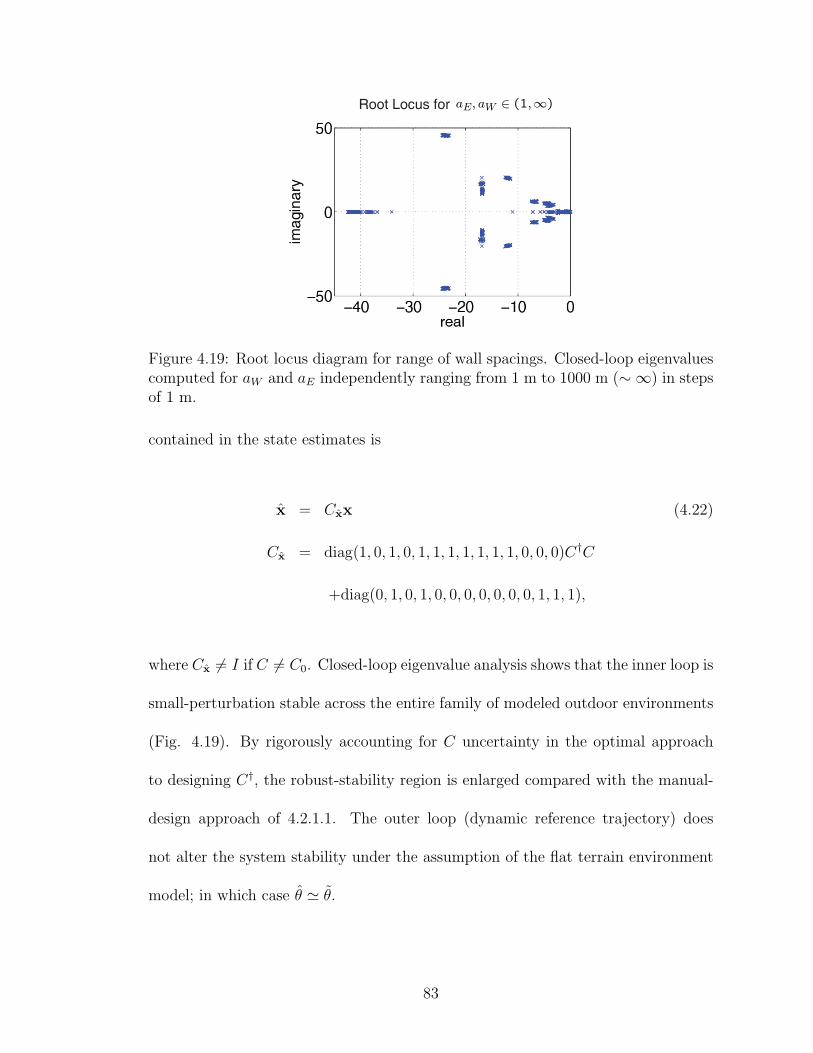
Root Locus for aE; aW 2 (1;1)

Figure 4.19: Root locus diagram for range of wall spacings. Closed-loop eigenvaluescomputed for aW and aE independently ranging from 1 m to 1000 m (∼ ∞) in stepsof 1 m.

contained in the state estimates is

x = Cxx (4.22)

Cx = diag(1, 0, 1, 0, 1, 1, 1, 1, 1, 1, 1, 0, 0, 0)C†C

+diag(0, 1, 0, 1, 0, 0, 0, 0, 0, 0, 0, 1, 1, 1),

where Cx 6= I if C 6= C0. Closed-loop eigenvalue analysis shows that the inner loop is

small-perturbation stable across the entire family of modeled outdoor environments

(Fig. 4.19). By rigorously accounting for C uncertainty in the optimal approach

to designing C†, the robust-stability region is enlarged compared with the manual-

design approach of 4.2.1.1. The outer loop (dynamic reference trajectory) does

not alter the system stability under the assumption of the flat terrain environment

model; in which case θ ' θ.

83

4.2.2.3 Simulation

Optic Flow Sensing and Computation

This section describes the methodology for simulating the micro helicopter in

a cluttered urban environment (Fig. 4.20). Greater maneuvrability and a lower

forward speed, compared with the fixed-wing UAV of Section 4.2.1, permit naviga-

tion of a more complex environment with more severe initial conditions. The same

camera setup is employed (Fig. 4.21) but is run at 60 fps for optic flow computation

at 800 image points. The points are distributed in a u-v spherical grid with constant

angular spacing between nodes, and are mapped from a virtual sphere surface to

the flat cameras via geometric projection (Appendix A.2). The optic flow measure-

ments are mapped back to the sphere (Eq. (A.7)), then de-sampled from 800 to

200 by unweighted averaging of ‘square’ groups of four adjacent nodes, with outlier

rejection to reduce noise. The simulation process is illustrated in Fig. 4.22.

To demonstrate robustness with respect to initial conditions, a monte carlo

approach was employed. 20 initial headings and (x,y) locations were generated using

a uniform distribution, excluding parts of the environment covered by buildings.

Results

Fig. 4.23 shows that from all initial conditions the helicopter is able to suc-

cessfully avoid the obstacles while maintaining a target height of 1 m above the

ground. This is achieved almost entirely with optic-flow-based measurements, with

the exception of the independent pitch angle, altitude and actuator-related state

measurements.

84

A

B

C

Figure 4.20: 3-D simulation environment.

Figure 4.21: Sampling the optic flow field: projections of camera boundaries on toright and left hemispheres of the sphere.

85

Grab Images

from 6

Cameras

Gaussian

Image Blur

Lucas-Kanade

Optic Flow

(at 800 pixel

coordinates)

Spatial Block

Averaging &

Outlier Rejec-

tion (800→200)

Wide-Field

Integration

Combine WFI

and Sensor

Measurements

ux UAV

Kinematics

& Dynamics

Visual

Environment

Compute

Reference

Trajectory

_Q

xref

Compute

Controls

Wide Field Integration & Control

Optic Flow Measurement

x

¡K(x¡ xref)

Figure 4.22: Spherical WFI simulation process diagram.

There are several instances where the helicopter heads back toward the build-

ings after clearing the obstacle course, but this is a reaction to the large sky-dome

that surrounds the environment (Fig. 4.20C). Fig. 4.24E shows the helicopter climb-

ing over a box completely obstructing its path, which is made possible by the adjust-

ment of target altitude. The terrain pitch angle spikes as the helicopter approaches

the box, which pushes the target altitude up, forcing the vehicle to temporarily

track an altitude-above-ground greater than 1 m in order to more safely approach

the upcoming terrain. Restricting the measurement grid to the lower hemisphere

(Figs. 4.24C and D) resulted in roughly similar performance, but eventual deviation

in trajectories due to differences in the y and ψ estimates. The full measurement

grid covers the entire height of the buildings thus the vehicle has stronger and earlier

warning of lateral obstacles compared with the reduced-FOV lower hemisphere grid.

86

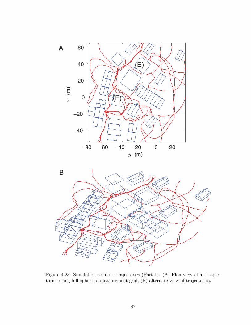
−80 −60 −40 −20 0 20

−40

−20

0

20

40

60

(m)

(m)

A

B

(E)

(F)

y

x

Figure 4.23: Simulation results - trajectories (Part 1). (A) Plan view of all trajec-tories using full spherical measurement grid, (B) alternate view of trajectories.

87

Full Measurement Grid

Lower Hemisphere GridC

D

E

F

−80 −60 −40 −20 0 20

−20

0

20

40

60

80

(m)

(m)

Full Measurement Grid

Lower Hemisphere Grid

−2−1

0

(m)

−2−1

0

(m)

−2−1

0

(m)

z

y

zz

x

Figure 4.24: Simulation results - trajectories (Part 2). (C) Plan view comparisonbetween spherical measurement grid and half-sphere grid for a single initial condi-tion, (D) side view comparison during navigation over a 0.5 m box, (E) 1 m box,(F) 1 m ramp.

67 68 69 70 71 72 73

0.4

1

1.6

(m

/s)

67 68 69 70 71 72 73

−0.6

0

0.6

(m

/s)

67 68 69 70 71 72 73

−0.6

0

0.6

time (s)

(m

/s)

67 68 69 70 71 72 73−3

0

3

(r

ad

/s)

67 68 69 70 71 72 73−3

0

3

(r

ad

/s)

67 68 69 70 71 72 73−3

0

3

time (s)

(r

ad

/s)

target

measured

true

uv

w

pq

r

Figure 4.25: Speeds, rates and optic-flow-extracted measurements for the full spher-ical measurement grid case (Fig. 4.23C) during a 90 turn.

88

67 68 69 70 71 72 73−1

0

1

(m)

67 68 69 70 71 72 73

−0.6

0

0.6

time (s)

(m)

)

)

67 68 69 70 71 72 73−30

0

30

(deg)

67 68 69 70 71 72 73−30

0

30

(deg)

measured (w.r.t. terrain)

true (inertial frame)

target (inertial frame)

67 68 69 70 71 72 73−30

0

30

time (s)

(deg)

−180 −90 0 90 1800

45

90

135

180

Measured Flow, =68.884 s

azimuth (deg)

elevation (deg)

t

=68.884 =68.884

target (w.r.t. terrain)

measured (w.r.t. terrain)

true (inertial frame)

tt

yz

Áµ

Ã

Figure 4.26: Vehicle pose, WFI outputs and measured optic flow for the full sphericalmeasurement grid case (Fig. 4.23C during a 90 turn.

Figs. 4.25 and 4.26 show the states and measurements for part of the Fig.

4.24C trajectory (during the second major turn). The asymmetry in the optic flow

pattern that prompts an avoidance maneuver is evident from Fig. 4.26. Despite the

fact that the WFI delivers environment-sensitive state estimates, the measurements

still satisfactorily track the true quantities. The low noise levels are attributable to

the white-noise mitigation property of wide-field integration and the outlier rejection

step in the spatial filtering of optic flow measurements. The environment-related

scaling error in the φ estimate does not compromise roll stability, but the high gain

on the ψ and y does lead to oscillations from the feedback of finite noise.

89

Chapter 5

Control Theoretic Interpretation of Tangential Cells

Whilst Chapters 3 and 4 are concerned with deriving the optimal WFI weight-

ing patterns for controlling robotic platforms, this chapter examines the fixed di-

rectional templates ingrained into the tangential cells of insects. The analysis tech-

niques are the same, but the weighting patterns are now fixed, rather than being

freely designable. This chapter seeks to address (1) the estimation question: what

do tangential cell outputs encode, and (2) the control question: how can they give

rise to the navigational heuristics observed by behavioral biologists. These are ques-

tions to which biologists have long sought an answer [3], and the insight gained by

addressing this research gap will further the understanding of how the insect archi-

tecture can be effectively leveraged for MAVs.

The properties of tangential cells are more complex than the simple linear-

integrator analogue of Section 2.3, but the analogue still provides a useful theoretical

framework for analyzing the patterns. Section 5.1 investigates the above mentioned

research questions in a simplified planar context and Section 5.2 extends the anal-

ysis to 3-D, to examine the hypothesis proposed by biologists that tangential cells

are tuned to sense the insect’s fundamental dynamics modes [3]. Insect weighting

patterns, or directional templates, were obtained from published data [1, 2, 3] for

all available tangential cells of the blow fly Calliphora (Figs. 5.1 and 5.2).

90

−180 −90 0 90 1800

45

90

135

180

H1−Right Directional Template

(deg)

(

de

g)

−180 −90 0 90 1800

45

90

135

180

H2−Right Directional Template

(deg)

(

de

g)

−180 −90 0 90 1800

45

90

135

180

Hx−Right Directional Template

(deg)

(

de

g)

−180 −90 0 90 1800

45

90

135

180

HSN−Right Directional Template

(deg)

(

de

g)

−180 −90 0 90 1800

45

90

135

180

HSE−Right Directional Template

(deg)

(

de

g)

−180 −90 0 90 1800

45

90

135

180

dCH−Right Directional Template

(deg)

(

de

g)

−180 −90 0 90 1800

45

90

135

180

vCH Directional Template

(deg)

(

de

g)

Figure 5.1: Directional templates of right brain hemisphere Calliphora tangentialcells sensitive to primarily horizontal optic flow.

91

−180 −90 0 90 1800

45

90

135

180

V1−Right Directional Template

(deg)

(

de

g)

−180 −90 0 90 1800

45

90

135

180

VS1−Right Directional Template

(deg)

(

de

g)

−180 −90 0 90 1800

45

90

135

180

VS2−Right Directional Template

(deg)

(

de

g)

−180 −90 0 90 1800

45

90

135

180

VS3−Right Directional Template

(deg)

(

de

g)

−180 −90 0 90 1800

45

90

135

180

VS4−Right Directional Template

(deg)

(

de

g)

−180 −90 0 90 1800

45

90

135

180

VS5−Right Directional Template

(deg)

(

de

g)

−180 −90 0 90 1800

45

90

135

180

VS6−Right Directional Template

(deg)

(

de

g)

−180 −90 0 90 1800

45

90

135

180

VS7−Right Directional Template

(deg)

(

de

g)

−180 −90 0 90 1800

45

90

135

180

VS8−Right Directional Template

(deg)

(

de

g)

−180 −90 0 90 1800

45

90

135

180

VS9−Right Directional Template

(deg)

(

de

g)

−180 −90 0 90 1800

45

90

135

180

VS10−Right Directional Template

(deg)

(

de

g)

Figure 5.2: Directional templates of right brain hemisphere Calliphora tangentialcells sensitive to primarily vertical optic flow.

92

5.1 1-D Tangential Cell Directional Templates

In this section the 1-D WFI operator (4.2) is used as a tangential cell (TC)

analogue to characterize the information that is encoded by the azimuthal directional

templates of tangential cells that compose the horizontal system (HS). The loop

closure design techniques developed in Chapter 3 are applied to show how tangential

cell analogue outputs could be used to stabilize and navigate.

5.1.1 Decoding TC Patterns

To provide initial insight into the interpretation of tangential cell patterns and

their possible role in the visuomotor loop, we consider insect motion restricted to

the horizontal plane. Therefore, the directional templates for the horizontal cells

(H1, H2, Hx, HSN, HSE, HSS, dCH and vCH) for both the left (L) and right (R)

hemispheres are included in the analysis. If one further restricts optic flow mea-

surements to the equatorial plane, then only the azimuthal-equatorial components

of the spherical weighting patterns are required. Representative data points for the

tangential cell weighting patterns were obtained from published data for each cell,

smoothed with a Gaussian filter and converted to a continuous function of γ by

making a 12th order Fourier series approximation (e.g., Fig. 5.3). The resulting 16

weightings Fy = Fyi, i = 1, . . . , 16 are then normalized so that a perfect match

of the optic flow field with the weighting function will result in unity output.

To characterize the small signal content encoded by the azimuthal-equatorial

cell directional templates, the set of outputs 〈Q, Fyi〉 are linearized about the nominal

93

0 100 200 300

−1

−0.5

0

0.5

1

γ (deg)

dCH−Right Equatorial Weighting Function

0 100 200 300−1.5

−1

−0.5

0

0.5

1

1.5

γ (deg)

Hx−Left Equatorial Weighting Function

−180 −90 0 90 180

30

60

90

120

150

dCH-Right Directional Template

−180 −90 0 90 180

Hx-Left Directional TemplateA B

γ (deg)

(deg)

30

60

90

120

150

(deg)

γ (deg)

Figure 5.3: Extraction of equatorial-azimuthal flow sensitivity for a left and righthemisphere tangential cell; (A) 2-D directional templates (data extracted and re-plotted from [1, 2, 3]), (B) azimuthal flow component for equatorial ring.

94

pattern of optic flow induced on the retina for centered motion between two large

obstacles (the yaw-plane infinite tunnel environment parameterized in Table 2.1,

with θ = φ = 0). This optic flow pattern corresponds to an equilibrium state

of x0 = (y0, ψ0, u0, v0, ψ0) = (0, 0, uref , 0, 0). The resulting observation equation

y = Cx is given by

H1R

H1L

H2R

H2L

HxR

HxL

HSNR

HSNL

HSER

HSEL

HSSR

HSSL

dCHR

dCHL

vCHR

vCHL

=

−0.50 −0.09 −0.49 0.09 1.000.50 0.09 −0.49 −0.09 −1.00−0.31 −0.17 −0.30 0.17 0.870.31 0.17 −0.30 −0.17 −0.87−0.48 −0.19 −0.47 0.19 0.860.48 0.19 −0.47 −0.19 −0.860.46 0.11 0.25 −0.11 −1.11−0.46 −0.11 0.25 0.11 1.110.56 0.11 0.24 −0.11 −1.21−0.56 −0.11 0.24 0.11 1.210.28 0.23 0.23 −0.23 −0.83−0.28 −0.23 0.23 0.23 0.830.56 0.14 0.05 −0.14 −1.25−0.56 −0.14 0.05 0.14 1.250.59 0.08 0.13 −0.08 −1.26−0.59 −0.08 0.13 0.08 1.26

x, (5.1)

where x = (u0

a2 y, u0

aψ, 1

au, 1

av, ψ) defines the state relative to the environment.

Inspection of (5.1) reveals that the cell output signals are functions of speed/depth

quantities, due to the nature of optic flow. The generated outputs are highly coupled

and no one cell weighting appears to provide direct measurement of any particular

speed/depth quantity as they have been parameterized. However, it is clear that a

relative forward speed estimate 1au can be obtained by summing the outputs of two

same-type cells from opposite hemispheres due to their symmetric sensitivity.

95

5.1.2 Static TC Output Feedback

From (5.1) it is not obvious how one could wire amplified TC output signals

to create stabilizing flight actuator commands. As shown in Chapter 3, the gain

selection task for a given set of tangential cell weighting patterns can be cast in a

rigorous framework in which traditional tools from control and information theory

can be leveraged to achieve the desired closed loop visual-based behaviors. Section

5.1.3.1 applies this process to a planar vehicle.

5.1.3 Experimental Validation

In the following section the methodology for achieving reflexive navigation be-

havior based on tangential cell outputs is experimentally demonstrated on a wheeled

vehicle (see 4.1.1.3 for details of the platform).

5.1.3.1 Feedback Synthesis

The angular velocity input ur is intended to generate commands to reflexively

maneuver the vehicle between objects in the surrounding environment. Following

(3.6), the output feedback is implemented as u = Ky where gains K = KC† are

applied to outputs

yi(x) = ∆γ

K∑j=1

Q(γj,x) Fyi(γj), (5.2)

which are computed from the K instantaneous measurements of optic flow Q and

the fixed set Fy = Fyi(γj), i = 1, . . . , M of tangential cell weightings.

To select the inversion C†, several sets of weightings are considered for com-

parison: (a) feedback based on 4 TC weighting patterns selected to maximize Fisher

information in the absence of noise statistics (i.e., least squares (LS) estimates), (b)

96

Weighting Function_Q! Ã Weighting Function_Q! y

0 100 200 300

−4

−2

0

2

4

γ (deg)

4 Cells (LS)

16 Cells (LS)

16 Cells (MV)

0 100 200 300−3

−2

−1

0

1

2

3

γ (deg)

4 Cells (LS)

16 Cells (LS)

16 Cells (MV)

Figure 5.4: State extraction pattern Fx = C†F comparison for control-relevantstates and three different tangential cell weighting function set selections.

feedback of all 16 TCs using the least squares estimates (Rw = I), and (c) feedback

of all 16 TCs using the minimum variance (MV) estimates (Rw,ij = ∆γ σ2η 〈Fyi

, Fyj〉,

simplified from the full sphere version (3.15)). The resulting state extraction pat-

terns Fx = C†Fy are plotted in Fig. 5.4. The 4 cell case represents the minimum

number of TCs required to guarantee C is full rank, and hence existence and unique-

ness of a solution to (3.7). Note that the sideslip velocity v = 0 for a wheeled vehicle.

If this were not the case then out-of-plane optic flow measurements and a pattern

with out-of-plane sensitivity would be required to maintain full rank of the mea-

surement model.

The chosen state feedback matrix is K = [Ky, Kψ, 0, 0], and the ratio of gains

Ky : Kψ for the trials shown was selected to be 2.25 : 1 to balance closed loop

overshoot and rise time. This results in gains at the tangential cell level presented

in Table 5.1. Equivalently, the same feedback could be implemented with a single

weighting pattern u = 〈Q, Fu〉 (Fig. 5.5) that represents a direct mapping between

optic flow sensors and the angular velocity command.

97

Weighting Function_Q! u

0 100 200 300−300

−200

−100

0

100

200

300

γ (deg)

4 Cells (LS)

16 Cells (LS)

16 Cells (MV)

Figure 5.5: Direct optic flow to actuator pattern Fu = KC†Fy comparison for threedifferent tangential cell weighting function set selections.

5.1.3.2 Results

The closed loop implementation was tested in two environments; a bent corri-

dor (Fig. 4.5A), and a cluttered field of large obstacles (Fig. 5.6). In the cluttered

environment two different initial conditions are used to evaluate performance. Trials

were repeated 10 times.

Fig. 5.7A-C shows that the vehicle successfully navigates the tunnel environ-

ment using all three inversions. The only clear trend is that 4-cell LS feedback avoids

overshoot during the initial condition recovery and executes a sharper turn at the

90 bend. The reason is that the 4-cell feedback is fundamentally biased toward

detecting off-nominal flow on the front-left and rear-right of the vehicle (see the ψ

sensitivity function asymmetry in Fig. 5.4). During the initial recovery, the presence

of the 90 bend downrange causes reduced optic flow on the vehicle’s front-right.

The robot does not respond to the optic flow perturbation, due to reduced sensitiv-

ity in this region, and reacts as if it were in a straight corridor. Implementation of

the 16-cell feedback (symmetric state sensitivity functions) demonstrates that the

optic flow perturbation leads to a reduced ψ-estimate which causes overshoot in the

centering behavior.

98

Figure 5.6: Cluttered obstacle field environment.

0 1 2

−2

−1

0

0 1 2

−2

−1

0

(m)

A B

0 1 2

−2

−1

0

C

D FE

−1 0 1

0

1

2

3

4

−1 0 1

0

1

2

3

4

−1 0 1

0

1

2

3

4

(m)y

x

(m)y (m)y

(m)

x

Figure 5.7: Vehicle trajectories (10 trials) and mean trajectory for tunnel with 90

bend and a cluttered obstacle field (forward speed u0 = 0.4 m/s); tangential cellgains determined from (A,D) 4-cell LS, (B,E) 16-cell LS, (C,F) 16-cell MV

99

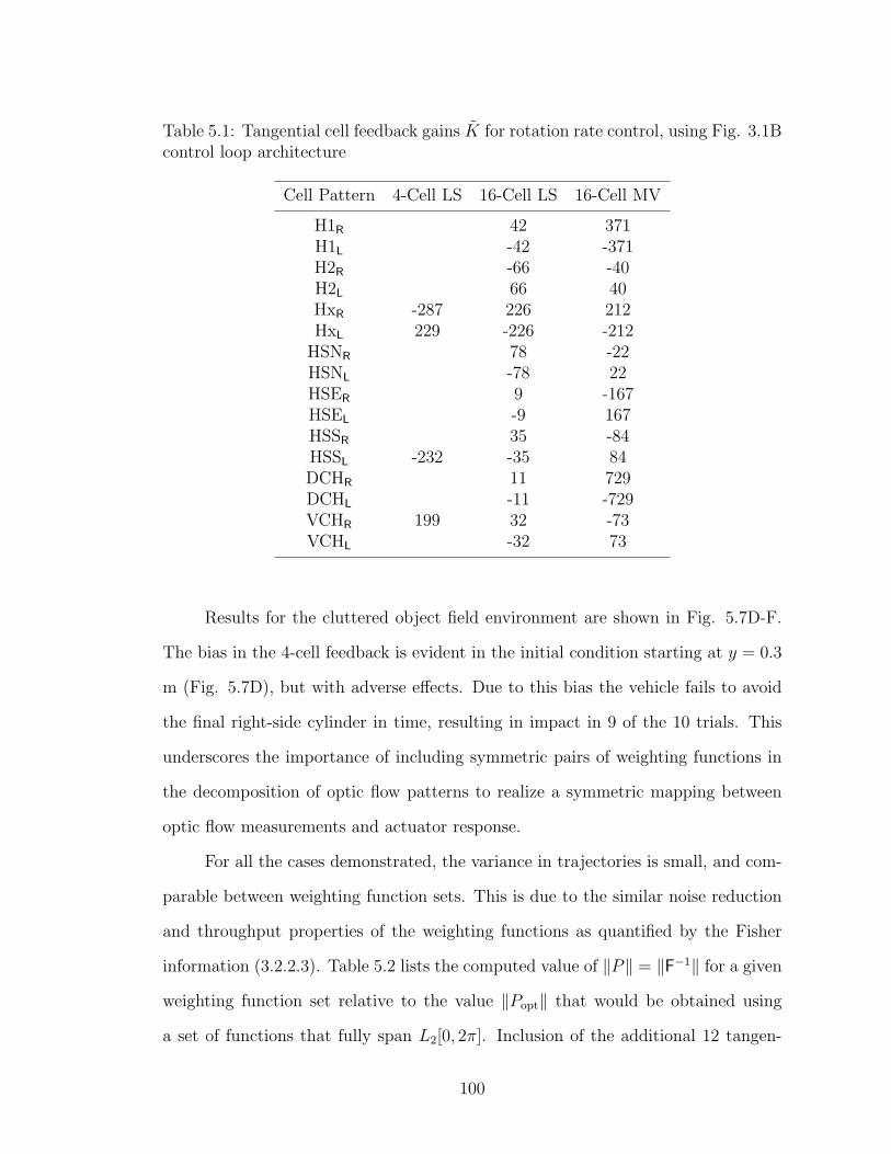
Table 5.1: Tangential cell feedback gains K for rotation rate control, using Fig. 3.1Bcontrol loop architecture

Cell Pattern 4-Cell LS 16-Cell LS 16-Cell MV

H1R 42 371H1L -42 -371H2R -66 -40H2L 66 40HxR -287 226 212HxL 229 -226 -212

HSNR 78 -22HSNL -78 22HSER 9 -167HSEL -9 167HSSR 35 -84HSSL -232 -35 84DCHR 11 729DCHL -11 -729VCHR 199 32 -73VCHL -32 73

Results for the cluttered object field environment are shown in Fig. 5.7D-F.

The bias in the 4-cell feedback is evident in the initial condition starting at y = 0.3

m (Fig. 5.7D), but with adverse effects. Due to this bias the vehicle fails to avoid

the final right-side cylinder in time, resulting in impact in 9 of the 10 trials. This

underscores the importance of including symmetric pairs of weighting functions in

the decomposition of optic flow patterns to realize a symmetric mapping between

optic flow measurements and actuator response.

For all the cases demonstrated, the variance in trajectories is small, and com-

parable between weighting function sets. This is due to the similar noise reduction

and throughput properties of the weighting functions as quantified by the Fisher

information (3.2.2.3). Table 5.2 lists the computed value of ‖P‖ = ‖F−1‖ for a given

weighting function set relative to the value ‖Popt‖ that would be obtained using

a set of functions that fully span L2[0, 2π]. Inclusion of the additional 12 tangen-

100

tial cell measurements in the feedback loop only reduces the noise throughput by

a factor of 2/3. The span of the 16 cell measurement set is apparently sufficiently

large to capture the range of perturbations in the optic flow pattern for the selected

environments, and therefore the state estimate covariance is virtually identical to

that achievable if one had access to an infinite set of linearly independent sensitivity

patterns.

Table 5.2: Minimum estimate covariance (relative to the global optimum) as afunction of WFI weighting pattern set

Weighting Set σ(P )/σ(Popt)

Infinite Span of L2[0, 2π] 1.00016 Tangential Cells 1.0334 Tangential Cells 1.526

The Fisher information is also instructive for the analysis of performance in

terms of the extent of the field of view. Table 5.3 plots the computed value of

‖P‖ relative to the value ‖P360‖ that would be obtained using a full 360 FOV.

It is evident that the noise throughput is dramatically increased when the FOV is

restricted. Hence, the reduction of noise throughput is a possible rationale for the

coupling between adjacent vertical system (VS) cells [80] to increase a cell’s effective

FOV. The importance of a wide FOV for robust information extraction has been

well studied [28].

Table 5.3: Minimum estimate covariance as a function of field of view

FOV σ(P )/σ(P360)

360.0 1.0180.0 9.290.0 2.0 ×102

45.0 6.1 ×103

22.5 1.9 ×105

101

5.1.4 Discussion

The mathematical tangential cell analogue demonstrates how stabilizing feed-

back gains can be synthesized for any set of M linearly independent tangential

cell weighting patterns, providing that M ≥ n where n is the number of explicit

states in the optic flow model. Furthermore, the patterns required to achieve spe-

cific visual-based navigation are not unique; similar behaviors can be achieved with

quite different sets of weighting functions (Table 5.1). Hence, the only requirement

on selection of weighting function sets is that they are sufficiently different (inde-

pendent) from one another (a large collective span). This is closely related to recent

results from the field of signal compression and reconstruction, where the most effi-

cient method of signal encoding is to use random basis functions if one has no prior

model for the signal [81].

The findings in Section 5.1.1 help explain results from similar studies involving

use of tangential cells for estimation and control. State estimation was investigated

in [36], who suggested using a summation of same-type horizontal cell outputs for

forward speed estimation, and subtraction of same-type outputs for yaw rate or

sideslip. These claims are supported by inspection of (5.1). However, in [36] the

results were limited to unweighted two-cell signal combinations, which essentially

constitutes inversion of a non-full rank measurement set. No method is proposed

for decoupling yaw rate from sideslip, or from the proximity and orientation states

that are also embedded in the subtraction-method output signal. The visuomotor

analogue presented here provides a rigorous methodology for using tangential cell

weighting properties in closed loop feedback.

Closed-loop control was investigated in [46], where obstacle avoidance was

attempted in simulation using a comparison of the left and right HSE cell outputs.

While this was useful for obstacle detection during periods of non-rotation, it was

unsuccessful when applied as continuous feedback because the subtracted HSE signal

102

contains coupled measurements of multiple states. The actuator signal should indeed

include these quantities (yaw rate, sideslip, proximity and orientation), but they

need to be fused using appropriate stabilizing gains rather than in the inherent

ratios of the HSE pattern. Although in [46] a hi-fidelity neuronal-based model for

the wide-field integration was used, the primary information throughput remains

the same.

5.2 2-D Tangential Cell Directional Templates

In this section the 2-D WFI operator (2.17) is used to analyze the full spherical

tangential cell directional templates with respect to the information they provide

about the dynamical system of the insect. The hypothesis that tangential cells

encode the fundamental dynamics modes is investigated by correlating the cell di-

rectional templates with the optic flow induced by modal motion.

The response of a system to an arbitrary excitation can always be expressed

as a summation of its fundamental modal responses. Since these modal motions will

dominate the flight behavior of an insect, it has been hypothesized that insects align

their sensors to sense the modes directly [3]. To examine this claim, a rigid body

dynamics model of a hovering Drosophila (fruit fly) is employed, obtained in [82, 83]

by system identification of a hi-fidelity non-linear flapping model. The identified

model is linear for small perturbations about hover, contains embedded haltere

feedback to augment stability, and assumes that lateral and longitudinal dynamics

are decoupled. The natural modes of the state space system x = Ax + Bu are

found from the eigenvectors of A, and they determine the behavior of the unforced

system (u=0); The eigenvectors specify the direction in state space that the insect

moves when a particular mode is excited, and the eigenvalue contains information

about the stability of the mode. Also of interest is the state space direction in which

103

the system is forced by each actuator input, and these can be determined directly

from the columns of B. The natural and input modes are summarized in Tables

5.4 and 5.5; note that proximity quantities are absent from the modes because such

information is not encoded by optic flow in the hover case (due to low translational

velocities).

Table 5.4: Longitudinal Drosophila dynamics modes (SI units) in hover condition

Mode Name θ u w q Eigenvalue

NATURAL MODESLongitudinal Oscillatory -0.0251 0.0541 0.9948 -3.51

±0.0805i ±0.0205i ±11.26iFast Longitudinal Subsidence -0.0259 -0.0097 0.9996 -38.56

Slow Heave 1.0000 -4.65INPUT MODESStroke Amplitude -1.0000

Stroke Plane Angle 0.0073 -1.0000Wing Oscillation Center 0.0021 1.0000

Table 5.5: Lateral Drosophila Dynamics Modes (SI units) in hover condition

Mode Name φ v p r Eigenvalue

NATURAL MODESRoll/Yaw Subsidence 0.0012 -0.0001 -0.2114 0.9774 -170.89Roll/Yaw Oscillatory 0.0010 -0.0027 0.1430 0.9886 -3.74

±0.0067i ±0.0012i ±0.0467i ±22.03iYaw Subsidence -0.0002 0.0180 -0.9998 -79.31INPUT MODES

Stroke Amplitude Diff. 0.0007 -1.0000Stroke Plane Diff. -1.0000

The optic flow induced by a particular mode of motion can be determined by

setting the state x to the applicable modal vector v from Table 5.4 or 5.5 and ap-

plying the algebraic model (2.3), assuming a form for the environment; 1 m sphere

104

assumed here (a simplification of (2.15)). Oscillatory modes contain complex com-

ponents, but these are ignored in determining the mode-induced optic flow patterns,

Fig. 5.8, as they do not affect the state space motion direction.

If tangential cell outputs are indeed tuned to provide direct static measure-

ments of natural and/or input modes, there should be strong correlation between the

TC directional templates Fyj(Figs. 5.1 and 5.2) and the mode-induced optic flow

patterns Fvi(Fig. 5.8). This comparison can be quantified with the 2-D WFI oper-

ator, by performing a spatial inner product between the two patterns on L2(S2,R2).

The absolute value of the scalar output gives an indication of the correlation Cji

between the patterns;

Cji = |〈Fvi,Fyj

〉|. (5.3)

Patterns F are pre-normalized such that their auto-correlation is unity, i.e., 〈Fk,Fk〉 =

1. Due to linearity of the WFI operator, (5.3) is equivalent to a normalized vector

dot product between row j of the observation matrix C (i.e., cTj ) and the modal

vector vi;

Cji = Ni|cj · vi|, (5.4)

where Ni is the factor used to normalize the Fvipattern and cj comprises the

linearized information embedded in tangential cell output yj obtained via an in-

ner product between the optic flow model and the TC directional template, yj =

〈Q,Fyj〉. Eq. (5.4) is the standard method of checking if mode i is observable with

measurement j. If Cji = 0 the mode is not observable from the particular tan-

gential cell output. If Cji = 1, the tangential cell directional template is perfectly

tuned to provide a direct measurement of the mode. Table 5.6 lists the computed

105

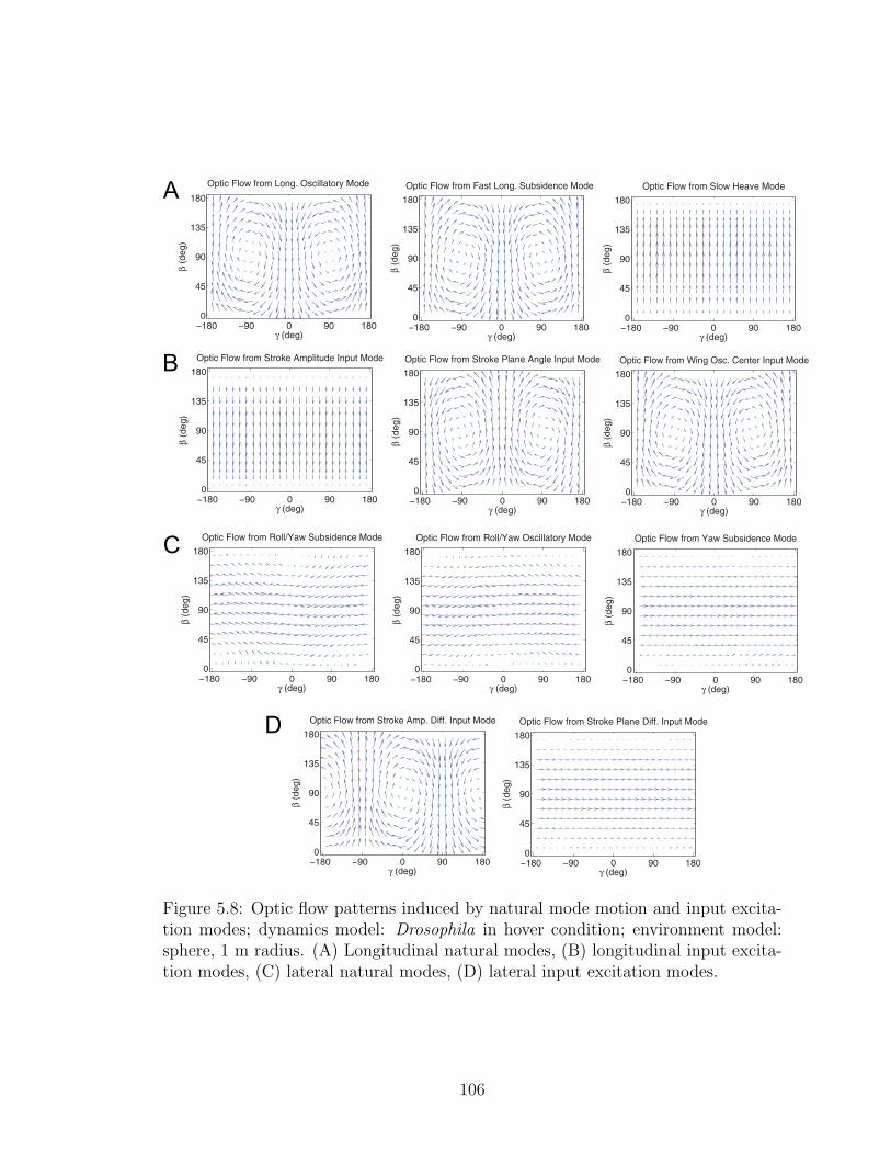
−180 −90 0 90 1800

45

90

135

180

Optic Flow from Long. Oscillatory Mode

(deg)

(

de

g)

−180 −90 0 90 1800

45

90

135

180

Optic Flow from Fast Long. Subsidence Mode

(deg)

(

de

g)

−180 −90 0 90 1800

45

90

135

180

Optic Flow from Slow Heave Mode

(deg)

(

de

g)

−180 −90 0 90 1800

45

90

135

180

Optic Flow from Stroke Amplitude Input Mode

(deg)

(

de

g)

−180 −90 0 90 1800

45

90

135

180

Optic Flow from Stroke Plane Angle Input Mode

(deg)

(

de

g)

−180 −90 0 90 1800

45

90

135

180

Optic Flow from Wing Osc. Center Input Mode

(deg)

(

de

g)

−180 −90 0 90 1800

45

90

135

180

Optic Flow from Roll/Yaw Subsidence Mode

(deg)

(

de

g)

−180 −90 0 90 1800

45

90

135

180

Optic Flow from Roll/Yaw Oscillatory Mode

(deg)

(

de

g)

−180 −90 0 90 1800

45

90

135

180

Optic Flow from Yaw Subsidence Mode

(deg)

(

de

g)

−180 −90 0 90 1800

45

90

135

180

Optic Flow from Stroke Amp. Diff. Input Mode

(deg)

(

de

g)

−180 −90 0 90 1800

45

90

135

180

Optic Flow from Stroke Plane Diff. Input Mode

(deg)

(

de

g)

B

A

D

C

Figure 5.8: Optic flow patterns induced by natural mode motion and input excita-tion modes; dynamics model: Drosophila in hover condition; environment model:sphere, 1 m radius. (A) Longitudinal natural modes, (B) longitudinal input excita-tion modes, (C) lateral natural modes, (D) lateral input excitation modes.

106

correlations.

Table 5.6: Spatial inner product between tangential cell directional templates andoptic flow pattern induced by natural mode motion and input excitation modes.

Long.

Osc.

Fast

Long.

Sub.

Slow

Heave

Stroke

Amp.

Stroke

Plane

Angle

Wing

Osc.

Center

Roll /

Yaw

Sub.

Roll /

Yaw

Osc.

Yaw

Sub.

Stroke

Amp.

Diff.

Stroke

Plane

Diff.

H1 0.02 0.05 0.09 0.09 0.05 0.05 0.68 0.66 0.68 0.09 0.68

H2 0.03 0.06 0.07 0.07 0.05 0.05 0.62 0.61 0.63 0.05 0.63

Hx 0.06 0.03 0.02 0.02 0.03 0.04 0.55 0.53 0.55 0.08 0.54

HSN 0.17 0.19 0.05 0.05 0.19 0.19 0.70 0.73 0.73 0.07 0.73

HSE 0.01 0.03 0.13 0.13 0.02 0.02 0.82 0.80 0.82 0.08 0.82

dCH 0.28 0.29 0.33 0.33 0.29 0.29 0.62 0.71 0.68 0.25 0.68

vCH 0.31 0.30 0.26 0.26 0.30 0.30 0.75 0.64 0.70 0.33 0.70

V1 0.57 0.58 0.42 0.42 0.58 0.58 0.17 0.02 0.09 0.42 0.08

VS1 0.57 0.59 0.40 0.40 0.59 0.59 0.30 0.25 0.27 0.15 0.27

VS2 0.49 0.50 0.52 0.52 0.50 0.50 0.08 0.02 0.02 0.27 0.02

VS3 0.44 0.45 0.54 0.54 0.45 0.45 0.07 0.05 0.00 0.35 0.00

VS4 0.10 0.10 0.62 0.62 0.10 0.10 0.15 0.08 0.03 0.64 0.01

VS5 0.09 0.09 0.62 0.62 0.09 0.09 0.13 0.09 0.01 0.65 0.00

VS6 0.03 0.03 0.59 0.59 0.03 0.03 0.05 0.19 0.08 0.66 0.10

VS7 0.33 0.33 0.52 0.52 0.33 0.33 0.03 0.18 0.09 0.57 0.10

VS8 0.51 0.52 0.39 0.39 0.52 0.52 0.04 0.20 0.13 0.46 0.14

VS9 0.53 0.54 0.44 0.44 0.54 0.54 0.08 0.06 0.00 0.39 0.01

VS10 0.56 0.58 0.41 0.41 0.58 0.57 0.05 0.18 0.12 0.35 0.13

LONG. MODES LAT. MODESLONG. INPUTS LAT. INPUTS0.75 – 1.00

0.50 – 0.75

0.25 – 0.50

0.00 – 0.25

It is clear from Table 5.6 that all the modes are indeed observable via the tan-

gential cell output set. This also follows from the fact that C is full rank, therefore

the current state can be determined instantaneously from a single measurement vec-

tor y. Some cells do appear to be tuned well to sense particular modes, but there is

also significant residual components from other modes. As discussed in Section 5.1.4,

the directional template symmetry of contralateral same-type cells can be utilized

to isolate translational from rotary motion or longitudinal from lateral motion. By

positively combining same-type right and left hemisphere cell outputs, measurement

correlation with longitudinal modes is improved and the lateral mode components

are completely filtered out (Table 5.7). By negatively combining outputs, the reverse

effect is acheived (Table 5.8).

107

Table 5.7: Spatial inner product between positively combined (right plus left hemi-sphere, normalized) tangential cell directional templates and optic flow pattern in-duced by natural mode motion and input excitation modes.

Long.

Osc.

Fast

Long.

Sub.

Slow

Heave

Stroke

Amp.

Stroke

Plane

Angle

Wing

Osc.

Center

Roll /

Yaw

Sub.

Roll /

Yaw

Osc.

Yaw

Sub.

Stroke

Amp.

Diff.

Stroke

Plane

Diff.

H1 (R+L) 0.03 0.08 0.14 0.14 0.08 0.07 0.00 0.00 0.00 0.00 0.00

H2 (R+L) 0.05 0.10 0.13 0.13 0.09 0.09 0.00 0.00 0.00 0.00 0.00

Hx (R+L) 0.10 0.04 0.03 0.03 0.05 0.05 0.00 0.00 0.00 0.00 0.00

HSN (R+L) 0.37 0.42 0.12 0.12 0.42 0.41 0.00 0.00 0.00 0.00 0.00

HSE (R+L) 0.02 0.07 0.36 0.36 0.07 0.06 0.00 0.00 0.00 0.00 0.00

dCH (R+L) 0.57 0.59 0.68 0.68 0.59 0.59 0.00 0.00 0.00 0.00 0.00

vCH (R+L) 0.64 0.63 0.54 0.54 0.63 0.63 0.00 0.00 0.00 0.00 0.00

V1 (R+L) 0.71 0.72 0.53 0.53 0.72 0.72 0.00 0.00 0.00 0.00 0.00

VS1 (R+L) 0.64 0.66 0.44 0.44 0.66 0.66 0.00 0.00 0.00 0.00 0.00

VS2 (R+L) 0.55 0.56 0.58 0.58 0.56 0.56 0.00 0.00 0.00 0.00 0.00

VS3 (R+L) 0.53 0.54 0.65 0.65 0.54 0.54 0.00 0.00 0.00 0.00 0.00

VS4 (R+L) 0.14 0.14 0.87 0.87 0.14 0.14 0.00 0.00 0.00 0.00 0.00

VS5 (R+L) 0.12 0.13 0.89 0.89 0.13 0.13 0.00 0.00 0.00 0.00 0.00

VS6 (R+L) 0.04 0.04 0.84 0.84 0.04 0.04 0.00 0.00 0.00 0.00 0.00

VS7 (R+L) 0.46 0.47 0.74 0.74 0.47 0.47 0.00 0.00 0.00 0.00 0.00

VS8 (R+L) 0.69 0.70 0.53 0.53 0.70 0.70 0.00 0.00 0.00 0.00 0.00

VS9 (R+L) 0.70 0.71 0.58 0.58 0.71 0.71 0.00 0.00 0.00 0.00 0.00

VS10 (R+L) 0.73 0.74 0.52 0.52 0.74 0.74 0.00 0.00 0.00 0.00 0.00

LONG. MODES LAT. MODESLONG. INPUTS LAT. INPUTS0.75 – 1.00

0.50 – 0.75

0.25 – 0.50

0.00 – 0.25

From Table 5.7, V S5R + V S5L encodes the slow heave mode best, whilst

V S10R + V S10L encodes the remainder of the longitudinal modes, which are dom-

inated by pitch-axis rotation. These conclusions are intuitive from visual inspec-

tion of the cell directional templates (Fig. 5.2). Table 5.8 shows that H1R − H1L

best encodes the bulk of the lateral modes (dominated by yaw-axis rotation), whilst

V S6R−V S6L best encodes the stroke amplitude differential input mode (dominated

by roll-axis rotation). The V S cells exhibit a clear trend in modal correlation, and

this is because their directional templates are tuned to rotations about different

axes - all close to the equatorial plane [3]; the azimuthal location of the axis varies

approximately linearly with the cell number.

It is important to recognize that although the tangential cell patterns correlate

well with the mode-induced patterns, the cell outputs do not appear to provide direct

108

Table 5.8: Spatial inner product between negatively combined (right minus lefthemisphere, normalized) tangential cell directional templates and optic flow patterninduced by natural mode motion and input excitation modes.

Long.

Osc.

Fast

Long.

Sub.

Slow

Heave

Stroke

Amp.

Stroke

Plane

Angle

Wing

Osc.

Center

Roll /

Yaw

Sub.

Roll /

Yaw

Osc.

Yaw

Sub.

Stroke

Amp.

Diff.

Stroke

Plane

Diff.

H1 (R-L) 0.00 0.00 0.00 0.00 0.00 0.00 0.91 0.87 0.90 0.12 0.90

H2 (R-L) 0.00 0.00 0.00 0.00 0.00 0.00 0.77 0.75 0.77 0.07 0.77

Hx (R-L) 0.00 0.00 0.00 0.00 0.00 0.00 0.73 0.70 0.72 0.11 0.72

HSN (R-L) 0.00 0.00 0.00 0.00 0.00 0.00 0.78 0.82 0.81 0.07 0.82

HSE (R-L) 0.00 0.00 0.00 0.00 0.00 0.00 0.88 0.86 0.88 0.09 0.88

dCH (R-L) 0.00 0.00 0.00 0.00 0.00 0.00 0.71 0.82 0.78 0.29 0.79

vCH (R-L) 0.00 0.00 0.00 0.00 0.00 0.00 0.85 0.73 0.80 0.38 0.79

V1 (R-L) 0.00 0.00 0.00 0.00 0.00 0.00 0.28 0.04 0.15 0.70 0.14

VS1 (R-L) 0.00 0.00 0.00 0.00 0.00 0.00 0.65 0.54 0.60 0.32 0.59

VS2 (R-L) 0.00 0.00 0.00 0.00 0.00 0.00 0.17 0.04 0.05 0.59 0.04

VS3 (R-L) 0.00 0.00 0.00 0.00 0.00 0.00 0.12 0.10 0.00 0.63 0.01

VS4 (R-L) 0.00 0.00 0.00 0.00 0.00 0.00 0.21 0.11 0.04 0.91 0.02

VS5 (R-L) 0.00 0.00 0.00 0.00 0.00 0.00 0.19 0.13 0.01 0.91 0.00

VS6 (R-L) 0.00 0.00 0.00 0.00 0.00 0.00 0.06 0.26 0.12 0.92 0.13

VS7 (R-L) 0.00 0.00 0.00 0.00 0.00 0.00 0.04 0.25 0.12 0.81 0.14

VS8 (R-L) 0.00 0.00 0.00 0.00 0.00 0.00 0.06 0.30 0.20 0.68 0.21

VS9 (R-L) 0.00 0.00 0.00 0.00 0.00 0.00 0.12 0.09 0.00 0.60 0.01

VS10 (R-L) 0.00 0.00 0.00 0.00 0.00 0.00 0.08 0.28 0.19 0.56 0.20

LONG. MODES LAT. MODESLONG. INPUTS LAT. INPUTS0.75 – 1.00

0.50 – 0.75

0.25 – 0.50

0.00 – 0.25

isolated measurements of individual modes, partly due to the fact that some modes

are highly coupled. The input excitation modes are also highly coupled to the

natural modes, which is logical for control purposes but prevents them from being

seperately observed. The analysis technique of Section 3.2.3 could be applied to

derive weighting patterns that do output modal measurements, but Tables 5.6-5.8

do not suggest that tangential cells perform this functionality. A post-processing

stage would be required to extract modal estimates from the TC outputs if mode-

space feedback control is desired. However, as was shown in Section 5.1.3, direct

static linear feedback of tangential cell outputs is sufficient to stabilize a vehicle.

The obvious limitation of this study is that we are attempting to correlate

the Drosophila dynamics modes with Calliphora tangential cell data. This is due

to the availability of published data, but the fundamental conclusions are unlikely

109

to change; i.e., system observability and the advantages of combining same-type

cell outputs from opposite hemispheres. It should also be noted that the modes

determined from the model are dominated by rotation motion. That is, a perturbed

Drosophila will apparently respond with significant rotation motion but very small

translations. The dynamics model has not been confirmed experimentally, thus it is

possible that the true modes may induce more translational optic flow, which some

tangential cells are better tuned to. If a dynamics model can be obtained for forward

flight, then the system modes will also contain proximity and orientation quantities.

It is of significant interest to examine how well the tangential cells encode these.

The above limitations prevent absolute conclusions as to the accuracy of the

central hypothesis. However, the high correlation values (0.73 - 0.92) between left-

right cell combinations and the dynamics modes provides the first mathematically-

grounded evidence that tangential cells do deliver (coupled) measurements of funda-

mental modes. The most important lesson from this Chapter is that any set of WFI

weighting patterns, with sufficiently large span, can be used to close the visuomotor

loop.

110

Chapter 6

WFI Algorithm Summary

For archival convenience and clarity, this chapter summarizes the proposed

sensor weighting pattern design technique and the real-time implementation of WFI-

based control. The concepts developed in Chapters 3 are presented again in a step-

by-step recipe format, without the theory, to simplify implementability on future

platforms.

The utility of this instruction manual is broader than just a guideline for

extracting behaviorally relevant information from spatially-distributed optic flow

measurements. It can in fact be applied to any type of distributed sensing array

by substituting the optic flow model with a model of the applicable sensor. Other

possible applications are electrolocation (detection of objects by perturbation in the

electric field) [92] and velocity-field sensing (using arrays of insect-like hair sensors)

[93].

6.1 WFI-Based Controller Design

The offline procedure for static linear WFI-based compensator design is given

below.

1. Define a set of measurement/grid points spatially distributed over the sphere

(or a potentially disconnected subset of the sphere).

2. Define a set of weighting patterns Fy with a preferably large span.

3. Define a parameterized environment model (e.g. (2.10) or (2.15)) and specify

the extremum values for the distance/structure parameters.

111

4. Define a nominal, equilibrium, trajectory x0.

5. For each extreme environment...

(a) Use the algebraic optic flow model, with state x0, to compute the optic

flow at each grid point Q(x0, γk, βk).

(b) For each state xi...

i. Perturb the state by a small δ and re-compute optic flow at each grid

point Q(x0 + δxi, γk, βk).

ii. Element i of the optic flow Jacobian (linearized about x0), at grid

point (γk, βk), is Qlin,xi(γk, βk) = Q(x0+δxi,γk,βk)−Q(x0,γk,βk)

δ.

iii. For each weighting pattern Fyj, perform Wide-Field Integration of

Qlin,xiover measurement grid to obtain observation matrix entry

Cji = 〈Qlin,xi,Fyj

〉. WFI operations should be performed using Eq.

(A.9), (A.10), or (A.11) depending on the grid type.

6. Compute C0 by averaging the C matrices for each extreme environment.

7. Compute the output noise covariance matrix Rw using (3.15) and the model

uncertainty penalty matrix RδC using (3.17).

8. Compute the mapping of WFI outputs to states, C†, using (3.9).

9. If the task permits flexibility to design weighting patterns freely, the weighting

patterns Fx that map optic flow measurements to state estimates are obtained

with (3.20).

10. Determine which states you wish to include in the feedback loop then use a

linear control tool (i.e., output LQR) to design the state feedback gain matrix

K.

112

11. If the task permits flexibility to design weighting patterns freely, the weighting

patterns Fu that map optic flow measurements to actuator commands are

obtained with (3.5). If not, actuator commands can be produced by control

law (3.2) using the original weighting patterns, with output feedback gain

matrix K = KC†.

6.2 Real-time Algorithm Implementation

In real-time, control input formulation requires just 2K multiplications and

additions per actuator. If one considers each of the K optic flow measurement points

as a sensor, then the computational requirements of the controller are identical to

that of a linear output feedback operation (i.e., a P × 2K matrix multiplication,

where P is the number of actuators). The recommended implementation is outlined

below.

1. Pre-load the WFI weighting patterns Fj (either exact values or reconstructed

via a spherical harmonic approximation)

2. Convert to camera-frame Cartesian weightings CF = F xc(γ, β), F yc(γ, β),including corrections for flat camera distortions and optic flow units:

F xc(γk, βk)

F yc(γk, βk)

F zc(γk, βk)

=r IMAGEWIDTH

2 xc,max FPSRCBRT

LB

0

F β(γk, βk)j

F γ(γk, βk)j

, (6.1)

where relevant quantities are defined in Eq. (A.5), (A.1) and (A.8). Note that

F zc can be disregarded.

3. For every frame...

113

(a) Use an analog sensor or digital camera imagery to measure 2-D optic

flow at each grid node. If there is a means to identify poor optic flow

estimates (i.e., via a cost function) then this can be used to reject outliers

by deleting the grid node and computing WFI outputs by real-time least

squares inversion (Eq. (A.11)) or by using a finer raw grid and then

averaging adjacent blocks of estimates, whilst rejecting outliers, to obtain

a coarser grid for the WFI step.

(b) Compute WFI outputs 〈Q,C Fj〉 using Eq. (A.9), (A.10), or (A.11) de-

pending on the grid type. If (A.11) is used without real-time adjustments

to the grid, relevant matrices can be stored prior to the main loop.

(c) Sample other non WFI-based sensors if applicable.

(d) Formulate actuator inputs using (3.1) or (3.2) depending on the type of

weighting functions used.

(e) Low-pass filter the actuator commands to reduce sensor to actuator noise

throughput.

114

Chapter 7

Summary and Conclusions

This chapter summarizes key results, compares them to similar studies, and

examines the feasibility and limitations of the WFI method. Areas for future work

are also identified.

7.1 Feasibility

With regards to hardware availability, existing MAVs are capable of obtaining

attitude and angular rate estimates through use of gyros, accelerometers and mag-

netometers [84]. A pitch or roll sensor is therefore easily attainable, and light-weight

sonar sensors are available for measurement of height [84, 75]. Fixed-wing UAVs

can also measure forward speed using a Pitot tube. Therefore, the sensor-fusion in

the proposed control loops presented in this thesis are hardware-feasible. However,

rather than relying on optic flow for the majority of state measurements (as was

done in Section 4.2), an improved configuration might employ an on-board inertial

measurement unit (IMU) to provide attitude and rate measurements - due to its

superior accuracy. The niche for optic-flow-based sensing on MAVs is not accurate

state estimation but relative proximity and velocity estimation.

The camera configurations proposed in Section 4.2 are academic but a sim-

ilar feasible realization is certainly possible (see Section 7.5). Since lower hemi-

sphere measurements are generally sufficient, one could even use a single camera

and panoramic mirror [85].

Regarding versatility of the WFI navigation concept, it is important to note

that the proposed information-extraction method is not limited to the environment

115

models presented in this thesis. The simplified models are used only for designing

weighting patterns, which are relatively insensitive to the environment assumption;

the ellipsoid and infinite tunnel models lead to near-identical optimal weightings.

By regulating unwanted asymmetries in the optic flow pattern (perturbations from

the equilibrium pattern [68, 3]), the vehicle attempts to track an obstacle-symmetric

(centered) path through its world. This is precisely the navigational heuristic ob-

served in honeybees [26] and is a trait independent of environment structure or

spacing.

7.2 Limitations

The attractive potential of WFI is its low computational burden and suitabil-

ity for analog implementation [70]. The disadvantage is that the implementations

described in this thesis do not perform well in environments with large areas of

poor contrast - a limitation of the dynamic range of modern imaging devices. This

could potentially be overcome through use of adaptive analog imaging and/or differ-

ent optic flow algorithms (i.e., block matching). For this reason, most vision-based

navigation studies utilize feature detection/tracking [86, 55], but the associated com-

putational requirements are generally too large for implementation on MAV avionic

hardware (i.e., small fixed point processor) at high bandwidth.

Another flaw is the possibility of a collision course into a symmetric obstacle.

Fortunately, the chance is small because stability analysis and simulation results

show that such trajectories are unstable. There are several close encounters in Fig.

4.13, for example, but when the helicopter becomes near enough, small asymme-

tries become stronger, enabling an avoidance maneuver prior to impact. Despite

exclusion of a front-side wall from the environment model, the designed weighting

patterns are still useful in these near-head-on approaches. However, the instances

116

during symmetric approaches to building walls or corners (which generate minimal

optic flow) where proximity becomes unsafe suggest the need for an emergency turn

or continuous control capability based on feedback of a WFI-based x (frontal prox-

imity) estimate [87]. Insects avoid such collisions by detecting expansion patterns

in the optic flow field and then executing a rapid turn, known as a saccade [25].

This estimate pattern could be derived using the enclosed room environment model

(2.10). The inherent limitation is that small obstacles generate high frequency per-

turbations to the optic flow signal that are filtered out by WFI. For avoidance of

such obstacles (i.e., poles and wires), one could implement detection of these high

frequency anomalies or make use of a forward-pointing range finding sensor such as

sonar [88]. The WFI technique presented in this thesis is suited to avoidance of large

obstacles. For detection of small objects, insects make use of different small-field

processing mechanisms [89].

One limitation of the analysis and simulations is the assumption that objects

in the environment are static. Small moving objects will manifest as colored noise in

the optic flow signal, but will be largely filtered out in the WFI process. However,

large moving objects may significantly bias the WFI-extracted quantities. In [26] it

was shown that Honeybees respond to an adjacent wall moving in the direction of

flight by flying closer to it (as the optic flow induced by the wall is reduced). Whilst

this did not result in any collisions for the Honeybees, the effect of non-static large

objects (e.g. cars) on the navigational stability of the robotic analogues presented

in this thesis needs to be studied.

7.3 Comparison with Literature

To compare results with similar studies, the ability to successfully navigate

a cluttered field makes this study comparable with [90]. The centering behavior

117

demonstrated in Fig. 4.13 outperforms the optic-flow-controlled trajectories in [37]

because only lateral offset is controlled in that study, instead of offset and orien-

tation (see also the comparison made in Fig. 7.1). Similarly, the terrain-following

performance improves on [52, 53] for the same reason, but in the vertical plane.

An algorithm developed in [51] potentially offers more robust obstacle avoidance by

detecting impingements on a spherical tunnel, but assumes independent knowledge

of vehicle motion. [91] contains a highly successful experimental demonstration of

the WFI concept on a fixed-wing UAV, mirroring our simulation results, but lacks

a formal stability proof and a theoretical basis for weighting pattern selection.

Almost every experimental attempt to use optic flow for obstacle avoidance

has employed a WFI approach [37, 38, 39, 42, 43, 44, 45, 48, 49, 50, 52, 53]. Whilst

some are successful, none apply any mathematical grounding to the task of sensor

to actuator weighting pattern design. A typical approach is to subtract averaged

optic flow over a left-side camera from a right-side camera, which is equivalent to

a constant magnitude weighting on symmetric subsets of the sphere. The resulting

weighting pattern is intuitive, but the WFI output will embed yaw rotation rate,

which overshadows any indication of obstacle proximity and can destabilize the vehi-

cle. Even with the rotation component artificially removed, the benefits of utilizing

the theoretically justified approach developed in this thesis is clear from Fig. 7.1.

The left vs right patch weighting pattern is akin to a DC weighting, which does not

encode lateral orientation and therefore creates a stable but undamped centering

response. The feedback connection of tangential cell outputs in [46] also constitutes

a form of WFI, with an ad hoc sensor to actuator weighting pattern design. How-

ever, their experiment also would have been more successful with application of the

Section 5.1 methodology.

In terms of motion-estimation and terrain mapping, WFI does not provide

explicit information about environment structure, as in [54, 60], but it does enable

118

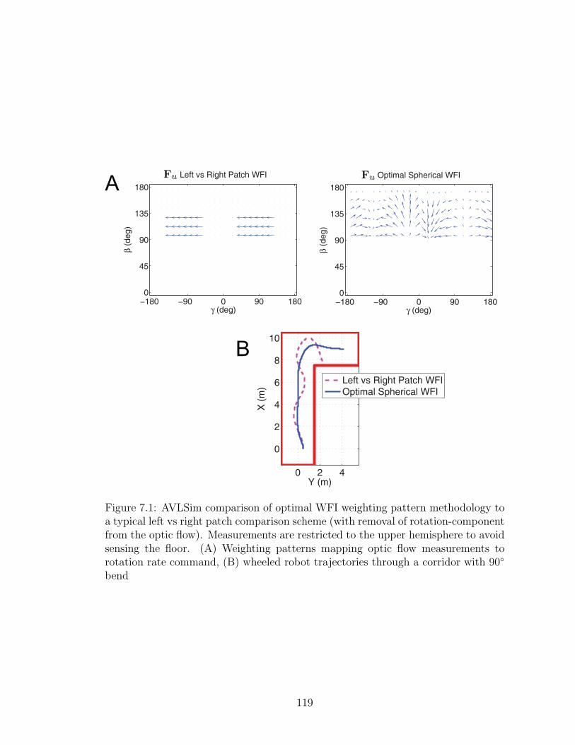
B

0 2 4

0

2

4

6

8

10

Y (m)

X (

m)

Left vs Right Patch WFI

Optimal Spherical WFI

−180 −90 0 90 1800

45

90

135

180

Optimal Spherical WFI

(deg)

(

de

g)

−180 −90 0 90 1800

45

90

135

180

Left vs Right Patch WFI

(deg)

(

de

g)

AFu Fu

Figure 7.1: AVLSim comparison of optimal WFI weighting pattern methodology toa typical left vs right patch comparison scheme (with removal of rotation-componentfrom the optic flow). Measurements are restricted to the upper hemisphere to avoidsensing the floor. (A) Weighting patterns mapping optic flow measurements torotation rate command, (B) wheeled robot trajectories through a corridor with 90

bend

119

motion-state extraction with noise-levels and accuracies similar to those reported

in [60, 62] and superior to those reported in [54]. Even lower noise is achieved

in [55], but high contrast feature tracking is employed, which is computationally

expensive. WFI is not an attempt to design the best vision algoritm, but to capitalize

on the benefits of vision-based servoing within the extreme computational/payload

constraints of minature air vehilces.

7.4 Conclusions

This thesis provides an important link between an insect’s neurophysiology

and its behavioral heuristics. By application of information theory it is shown what

tangential cells may be encoding, and through linear controller design it is shown

how an analogue to tangential cells can be used to stabilize a vehicle. This is the

first effort to mathematically link the properties of the insect visuomotor system to

the impressive flight behaviors we see everyday. More importantly, it shows how the

biological concept of converging massive noisy sensor arrays to a handful of flight

commands can be transitioned to 6-DOF engineered platforms.

The outcome of this thesis is a mathematical analogue to tangential cells which

can be directly applied to 6-DOF vehicles for robust obstacle avoidance and stability

augmentation. The approach presented here is not an attempt to precisely model

the feedback interconnections within insects; rather, it seeks to characterize the fun-

damental operational principle within a mathematical framework for transition to

engineered systems. Specifically, it is shown that the resulting feedback synthesis

task can be cast as a combined static state estimation and linear feedback control

problem. Additionally, the framework described herein provides a theoretically jus-

tified methodology for analysis and design of direct mappings between optic flow

measurements and actuator commands, which greatly simplifies implementation on

120

robotic platforms [70]. The techniques developed in this thesis can be directly uti-

lized for compensator design with any distributed sensing array type.

A list of key results from the thesis is presented below:

Chapter 2

1. Using an algebraic approximation of simple 3-D worlds, one can predict what

information is encoded in spatial patterns of optic flow. This allows us to apply

mathematical techniques to design weighting patterns that decode relevent

information from optic flow measurements.

Chapter 3

2. The task of designing WFI weighting patterns that linearly map a distributed

sensor array to actuator commands can be cast as a combined static state

estimation and linear feedback control problem. This allows incorporation of

robustness to noise, model uncertainty and dynamic performance objectives

into the static weighting patterns. Existence of solution is guaranteed if all

applicable constraints of the state feedback gain technique are satisifed and if

the initial trial set Fy contains m ≥ n linearly independent weighting patterns

such that the matrix of inner products between the weighting patterns and

the optic flow model Jacobian elements is full rank.

Chapter 4

3. A perturbation optic flow pattern, which is superimposed on the nominal

pattern when a state deviates from the nominal trajectory, is not necessarily

orthogonal to patterns induced by other states. This is also true when the

dynamics are transcribed to modal form. The static state extraction step in

the weighting pattern design process removes the effects of non-orthgonality,

filtering out information from unwanted states. However, the final weighting

pattern set is not necessarily orthogonal.

121

4. For an infinite planar tunnel, it was shown (for a wheeled robot) that the

closed-loop WFI output feedback system is large-perturbation stable about

a centered trajectory, with non-linear dynamics and outputs. The guaran-

teed stability region approaches that of the entire tunnel as the lateral offset

feedback gain becomes small and the ratio of the two gains becomes large.

5. By parameterizing a simple 3-D environment, and computing the observation

matrix Cx for all reasonable combinations of environment dimensional param-

eters, it was shown (for a fixed-wing UAV and a micro helicopter) that the

closed-loop WFI output feedback system is small-perturbation stable about a

centered trajectory for the entire family of modeled environments.

6. Different navigational behaviors (e.g. hover, landing, wall hug, centering) can

be acheived rapidly during flight by adjusting the target state. This mode

switch may also need to be accompanied with gain adjustment.

7. Experiments on a ground robot showed that WFI-based obstacle avoidance

was robust to initial conditions, optic flow measurement noise, and environ-

ment structure. Test failures, not shown here, only resulted during head-on

approaches to small obstacles (see discussion of limitations, Section 7.2).

8. Experiments on a micro quadrotor with 1-D WFI demonstrated that unde-

sirable performance constraints arise from side-slip motion when optic flow

measurements are limited to the equatorial circle. This follows from small-

perturbation stability analysis, and provides motivation for using 2-D WFI on

an increased measurement domain.

9. Optic flow measurements from three orthogonal planes provide sufficient data

to extract all proximity and motion states reliably via WFI. However, optic

flow measurements over the full sphere maximize robustness with respect to

122

measurement noise.

10. Monte Carlo simulations of a micro helicopter in an urban-like environment

verified closed-loop robustness to environment structure and spacing. From

a variety of initial conditions, the vehicle successfully avoided obstacles and

terrain anomalies whilst maintaining stable flight. Restriction of measure-

ments to the lower hemisphere reduced obstacle clearance distances but did

not compromise stability.

Chapter 5

11. Insect tangential cells do not appear to be tuned to provide isolated measure-

ments of individual motion/proximity states or fundamental dynamics modes,

but static output feedback design tools can be applied to generate the same

centering and clutter reponses observed in insects.

12. Within the WFI framework, the most important property of the tangential

cell directional templates is that their combined span is large, which reduces

noise throughput in the visuomotor system.

13. WFI requires a large field of view to keep noise throughput at manageable

levels. For lateral fields of view less than 180, noise throughput increases

dramatically.

14. Weighting patterns that map sensors to state estimates or sensors to actuators

are not unique. However, there exists a unique optimum given quantifiable

objectives such as noise minimization and dynamic performance. This result

also applies to stabilizing sets of output feedback gains.

Chapter 6

15. Real-time implementation of WFI-based control requires just four weighted

summations of 200 optic flow measurements per control update (for case study

123

4.2.2). Given the current lack of sensors with suitable mass and bandwidth

for MAVs, WFI implementations could provide an attractive alternative for

stability augmentation and collision avoidance in the field.

7.5 Future Work

Optic flow is a relative measure, thus the state estimates obtained in this study

are generally scaled combinations of speed/depth. In this thesis it has been shown

that these quantities are sufficient for regulating a safe optic flow pattern and hence

a safe trajectory. One complication of this is that pure WFI-based control will cause

the vehicle to regulate a lower altitude when obstacles are tightly spaced. From a

safety viewpoint this is undesirable, which is why an independent measurement of

z was assumed available in the micro-helicopter study (4.2.2). In contrast, it may

be beneficial to link forward speed with lateral obstacle spacing using a weighting-

pattern such as that shown in Fig. 2.4A to measure u. This strategy, requiring a

reduction in the uncertainty weighting ε, is of significant interest for future studies.

Optimality of the weighting patterns is also contigent on the noise covariance matrix

Rw, and future efforts should apply the stochastic analysis performed in [72] to (3.13)

to refine Rw.

There are several areas of WFI-related research at the University of Mary-

land’s Autonomous Vehicles Lab where progress has been made but the applicable

mechanisms have not yet been formalized. Firstly, it has been shown experimentally

that the frontal proximity x estimate can be used to scale the ψ feedback gain to

enhance avoidance of obstacles directly in front. However, this non-linear controller

has not yet received a formal design/analysis treatment. Secondly, vehicles that re-

quire high banking during maneuvres (fixed-wing UAVs) need active rotation of the

weighting patterns (or cameras) to keep their visual servoing sensitivities level with

124

the horizon. Without such compensation, the lateral proximity indicator reacts to

the ground during a turn and responds more weakly to actual obstacles. Compen-

sation algorithms have been designed and tested in simulation, but lack any formal

analysis. Insects use gaze stabilization, keeping their head level by rotating their

necks, and the responsible neuronal mechanisms closely resemble the architecture of

the tangential cells [94] analyzed in this thesis. A more rigorous investigation how

this concept can be transitioned to MAVs is warranted.

Experimental validation of the 2-D WFI techniques developed in Section 4.2

will soon be possible using Centeye’s Multiaperture Optical System (MAOS) (Fig.

7.2). This is a series of 2-D imaging arrays connected to analog VLSI / DSP hybrid

chips that perform optic flow computations. These feed to a small micro-processor

for the pooling of data and the WFI operations. Coverage of the entire sphere is

possible, and this should deliver a large improvement over the yaw-ring WFI used on

the quadrotor experiment (4.1.2). It will allow detection of out-of-plane obstacles,

decoupling of sideslip motion from the lateral orientation estimate, more reliable

estimation of body velocities (without the need for IMU fusion), and reduced noise

throughput to the actuators due to a greater field of view.

125

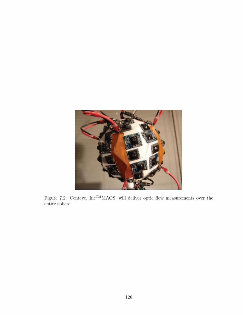
Figure 7.2: Centeye, IncTMMAOS; will deliver optic flow measurements over theentire sphere

126

Appendix A

Derivations

A.1 WFI Simplification using Linearized Optic Flow Model

Theorem

Let f(γ, β) and g(γ, β,x) be functions residing in L2(S2,R2). Define the

operation

y(x) =

∫ b(x)

a(x)

∫ d(x)

c(x)

g(γ, β,x) f(γ, β) sin β dβ dγ

and the linearization of y(x) about x = x0 as z(x) = y(x0) +∑

i∂y∂xi

(x0) (xi − xi0).

Then z(x) can be computed by

z(x) = y(x0) +∑

i

(xi − xi0)

∫ b(x0)

a(x0)

∫ d(x0)

c(x0)

∂g(γ, β,x)

∂xi

(x0) f(γ, β) sin β dβ dγ.

127

Proof

z(x) = y(x0) +∑

i

(xi − xi0)∂

∫ b(x)

a(x)

∫ d(x)

c(x)g(γ, β,x) f(γ, β) sin β dβ dγ

∂xi

∣∣∣∣∣x=x0

= y(x0) +∑

i

(xi − xi0)

∫ b(x)

a(x)

∫ d(x)

c(x)

(∂g(γ, β,x)

∂xi

f(γ, β)

+g(γ, β,x)∂f(γ, β)

∂xi

)sin β dβ dγ

∣∣∣∣∣x=x0

= y(x0) +∑

i

(xi − xi0)

∫ b(x0)

a(x0)

∫ d(x0)

c(x0)

∂g(γ, β,x)

∂xi

(x0) f(γ, β) sin β dβ dγ.

A.2 Flat-Camera to Sphere Mapping

The spherical grid points are mapped to individual camera pixels by the fol-

lowing method; note that a pin-hole camera model has been assumed.

1. For each camera, compute the direction cosine matrix RCB that brings body-

frame vectors into the local camera frame. We define the camera frame with

the x-axis pointing image-right and y pointing image-up, which leads to

RCB = R1(−π

2

)R3

(π

2

)R1(φc)R2(θc)R3(ψc). (A.1)

Ri refers to a Euler rotation matrix about axis i, and the camera yaw (ψc),

pitch (θc) and roll (φc) are the 3-2-1 Euler rotations relative to a zero-roll

camera pointing along the body xb-axis.

2. Define a measurement grid of spherical coordinates that covers the desired

swath to be used in the WFI. For each grid point, define its projection point

128

on the unit sphere in terms of Cartesian coordinates;

[er]B =

xb

yb

zb

=

cos γ sin β

sin γ sin β

cos β

. (A.2)

3. For each camera, compute the camera-frame xc, yc coordinate limits of the

viewable region boundaries - defined by the horizontal and vertical field of

views (αH and αV respectively). The camera is modeled as a flat rectangular

surface situated such that its center-point touches the unit sphere (Fig. A.1).

xc,max = tan−1 (αH/2) (A.3)

yc,max = tan−1 (αV /2).

4. For each camera, cycle through all grid points and compute the corresponding

camera frame coordinates by shifting the body-frame vector into the camera

frame. The body-frame vector length r must be recomputed for every possible

camera and grid point combination as it is the distance along the relevent

spherical coordinate vector to the geometric projection point on the applicable

camera surface.

[r]C = RCB [er]B r. (A.4)

Since the camera surface is assumed to be touching the unit sphere only at its

center, the zc coordinate (axis orthogonal to the camera plane) of a point on

the camera surface will always be -1. We can use this to solve the zc expression

129

eyb

exb

ezb

exceyc

°r

Camera

Plane

Camera

Surface

xc;max

yc;max

BC

Figure A.1: Projection of spherical coordinate grid on to flat imaging surface. Shownis an equatorial measurement node projected from the unit sphere to the camerasurface along vector r. The surface boundaries are defined by the horizontal andvertical field of views.

130

from (A.4) for r, in order to make the general (A.4) equation deterministic.

r =1

cos θc sin β cos (ψc − γ)− sin θc cos β. (A.5)

5. If the camera-frame coordinates for the grid point fall within the viewable

region of the camera (i.e. |xc| < xc,max, |yc| < yc,max, r > 0), then compute

the specific pixel coordinates and assign the grid point to be measured using

that camera:

PIXELCOLUMN =

(xc

xc,max

+ 1

)IMAGEWIDTH

2(A.6)

PIXELROW =

(yc

yc,max

+ 1

)IMAGEHEIGHT

2.

The camera-frame Cartesian optic flow estimates are mapped to the local

spherical frame L = er, eβ, eγ by the following method:

Qr

Qβ

Qγ

= RLBRTCB

∆xc

∆yc

0

xc,max 2 FPS

r IMAGEWIDTH(A.7)

RLB =

sβcγ sβsγ cβ

cβcγ cβsγ −sβ

−sγ cγ 0

. (A.8)

assuming small shifts (∆xc, ∆yc) between frames. The 1/r quantity converts linear

shift to angular units and compensates for the fact that the same rotation motion

will cause greater image shifts near the camera edges than at the center. Note that

radial flow Qr is ignored as it is merely a numerical artifact from the use of a flat

imaging device.

131

A.3 WFI Computation for Different Measurement Grids

To ensure accurate discretization of the continuous integral over the measure-

ment domain, the chosen grid node spacing must be accompanied with appropriate

weightings of nodes in the summation.

• If grid points have equal angular spacing (∆γ = ∆β) then

yj = ∆γ∆β

K∑

k=1

(Qγ(γk, βk) F γ

yj(γk, βk) + Qβ(γk, βk) F β

yj(γk, βk)

)sin β. (A.9)

• If grid points cover (approximately) equal solid angles (∆Ω ≈ constant), as in

the case of sub-divided icosahedral grid, then

yj = ∆ΩK∑

k=1

(Qγ(γk, βk) F γ

yj(γk, βk) + Qβ(γk, βk) F β

yj(γk, βk)

). (A.10)

• If grid points not consistently spaced, then select an orthonormal basis for

L2(S2,R) and define matrix G whose entries Gkf = Ff (γk, βk) correspond

to element f from the basis (e.g. spherical harmonic f). Considering the

azimuthal direction, define vector Vγ with entries Vγk = Fyj

(γk, βk) and X γ

with entries X γk = Qγ(γk, βk). Since both the weighting pattern and optic flow

can be approximated as a summation of elements from the orthonormal basis

(Vγk = GYγ and X γ

k = GZγ), the WFI inner product can be constructed as

the summation of the inner products between basis elements. To achieve a

good approximations, include spherical harmonics up to ∼10th order. Least

squares inversion is used to solve for the basis coefficients Yγ and Zγ, and the

132

inner product is extended to include both dimensions:

yj = (Yγ)TZγ + (Yβ)TZβ (A.11)

= (Vγ)T G(GT G)−T (GT G)−1GTX γ + (Vβ)T G(GT G)−T (GT G)−1GTX β.

133

Bibliography

[1] H. G. Krapp, R. Hengstenberg, and M. Egelhaaf. Binocular contributions tooptic flow processing in the fly visual system. Journal of Neurophysiology,85:724–734, 2001.

[2] H. G. Krapp, B. Hengstenberg, and R. Hengstenberg. Dendritic structure andreceptive-field organization of optic flow processing interneurons in the fly. Jour-nal of Neurophysiology, 79(4):1902–1917, 1998.

[3] G.K. Taylor and H.G. Krapp. Sensory systems and flight stability: What doinsects measure and why? Advanced Insect Physiology, 34:231–316, 2008.

[4] R. J. Wood, E. Steltz, and R. S. Fearing. Nonlinear performance limits for highenergy density piezoelectric bending actuators. In International Conference onRobotics and Automation. Barcelona, Spain, 2005.

[5] A. M. Hoover and R. S. Fearing. Fast scale prototyping for folded millirobots.In Robotics and Automation, 2008. ICRA 2008. IEEE International Conferenceon, pages 886–892, May 2008.

[6] R. J. Wood, S. Avadhanula, R. Sahai, E. Steltz, and R. S. Fearing. Microrobotdesign using fiber reinforced composites. ASME Journal of Mechanical Design,130(5), 2008.

[7] R. J. Wood, S. Avadhanula, R. Sahai, E. Steltz, and R. S. Fearing. Firsttakeoff of a biologially-inspired at-scale robotic insect. IEEE Trans. on Robotics,24(2):341–347, 2008.

[8] Aerius data sheet. [online], http://www.procerusuav.com/Downloads/DataSheets/AeriusMiniatureLaserRangefinder.pdf, Accessed 7/20/09.

[9] O. Amidi, Y. Mesaki, and T. Kanade. A visual odometer for autonomoushelicopter flight. Robotics & Autonomous Systems, August 1999.

[10] P. Gurfil and H. Rotstein. Partial aircraft state estimation from visual motionusing the subspace constraints approach. Journal of Guidance, Control, andDynamics, 24(5):1016–1028, 2001.

[11] S. Hrabar and G. S. Sukhatme. Omnidirectional vision for an autonomoushelicopter. In In IEEE International Conference on Robotics and Automation,pages 558–563, 2003.

[12] M. Garratt and J. Chahl. Visual control of an autonomous helicopter. InProceedings of the 41st Aerospace Sciences Meeting and Exhibit. AIAA 2003-460, Reno, NV, 2003.

134

[13] P. J. Garcia-Pardo, G. S. Sukhatme, and J. F. Montgomery. Towards vision-based safe landing for an autonomous helicopter. Robotics and AutonomousSystems, 38(1):19 – 29, 2002.

[14] J. Li and R. Chellappa. A factorization method for structure from planarmotion. IEEE Workshop on Motion and Video Computing, 2:154–159, January2005.

[15] B. K. P. Horn. Robot Vision. MIT Press and McGraw-Hill, Cambridge, MA,1986.

[16] E. R. Davies. Machine Vision: Theory, Algorithms, Practicalities. MorganKaufmann, San Francisco, CA, 2005.

[17] F. Kendoula, I. Fantoni, and K. Nonamib. Optic flow-based vision system forautonomous 3d localization and control of small aerial vehicles. Robotics andAutonomous Systems (in press), 2010.

[18] R. Beard, D. Kingston, M. Quigley, D. Snyder, R. Christainsen, W. Johnson,T. McLain, and MA Goodrich. Autonomous vehicle technologies for small fixed-wing uavs. Journal of Aerospace Computing, Information, and Communication,2:92–108, 2005.

[19] J. M. Grasmeyer and M. T. Keennon. Development of the black widow microair vehicle. In Proceedings of the 39th AIAA Aerospace Sciences Meeting andExhibit. 2001.

[20] M. A. Frye and M. H. Dickinson. Fly flight: A model for the neural control ofcomplex behavior. Neuron, 32(3):385–388, 2001.

[21] M. Egelhaaf, R. Kern, H. Krapp, J. Kretzberg, R. Kurtz, and A. Warzecha.Neural encoding of behaviourally relevant visual-motion information in the fly.Trends in Neurosciences, 25(2):96–102, 2002.

[22] A. Borst and J. Haag. Neural networks in the cockpit of the fly. Journal ofComparative Physiology A, 188(6):419–437, 2002.

[23] J. J. Gibson. The perception of the visual world. Houghton Mifflin, Boston,1950.

[24] C. T. David. Compensation for height in the control of groundspeed byDrosophila in a new, barber’s pole wind tunnel. Journal of Comparative Phys-iology, 147(4):485–493, 1982.

[25] L. F. Tammero and M. H. Dickinson. The influence of visual landscape onthe free flight behavior of the fruit fly Drosophila Melanogaster. Journal ofExperimental Biology, 205:327–343, 2002.

135

[26] M. V. Srinivasan, S. W. Zhang, M. Lehrer, and T. S. Collett. Honeybee nav-igation en route to the goal: Visual flight control and odometry. Journal ofExperimental Biology, 199(1):237–244, 1996.

[27] M. V. Srinivasan and S. W. Zhang. Visual motor computations in insects.Annual Review if Neuroscience, 27:679–696, 2004.

[28] J. J. Koenderink and A. J. van Doorn. Facts on optic flow. Biol. Cybern.,56(4):247–254, 1987.

[29] N. Franceschini, A. Riehle, and A. Le Nestour. Directionally selective motiondetection by insect neurons. In DG Stavenga and RC Hardie, editors, Facetsof Vision, pages 360–390. Springer-Verlag, Berlin, 1989.

[30] M. Egelhaaf and A. Borst. Motion computation and visual orientation in flies.Journal of Comparative Biochemistry Phisiology, 104(4):659–673, 1993.

[31] K. Hausen. Motion sensitive interneurons in the optomotor system of thefly, part i. the horizontal cells: Structure and signals. Biological Cybernetics,45:143–156, 1982.

[32] K. Hausen. Motion sensitive interneurons in the optomotor system of the fly,part ii. the horizontal cells: Receptive field organization and response charac-teristics. Biological Cybernetics, 46(1):67–79, 1982.

[33] R. Hengstenberg, K. Hausen, and B. Hengstenberg. The number and struc-ture of giant vertical cells (vs) in the lobula plate of the blowfly CalliphoraErythrocephala. Journal of Comparative Physiology, 149(2):163–177, 1982.

[34] H. G. Krapp and R. Hengstenberg. Estimation of self-motion by optic flowprocessing in single visual interneurons. Letters to Nature, 384:463–466, 1996.

[35] M. O. Franz and H. G. Krapp. Wide-field, motion-sensitive neurons andmatched filters for optic flow fields. Biological Cybernetics, 83:185–197, 2000.

[36] K. Karmeier, J. H. van Hateren, R. Kern, and M. Egelhaaf. Encoding ofnaturalistic optic flow by a population of blowfly motion-sensitive neurons.Journal of Neurophysiology, 96:1602–1614, 2006.

[37] S. Hrabar, G. S. Sukhatme, P. Corke, K. Usher, and J. Roberts. Combinedoptic-flow and stereo-based navigation of urban canyons for a uav. In Proceed-ings of the IEEE International Conference on Intelligent Robots and Systems.Edmonton, Canada, 2005.

[38] A. Beyeler, J.-C. Zufferey, and D. Floreano. 3d vision-based navigation forindoor microflyers. In Proceedings of the IEEE International Conference onRobotics and Automation. Roma, 2007.

136

[39] S. Griffiths, J. Saunders, A. Curtis, T. McLain, and R. Beard. Obstacle andTerrain Avoidance for Miniature Aerial Vehicles (in Book: Advances in Un-manned Aerial Vehicles), volume 33. Springer Netherlands, 2007.

[40] M. O. Franz and H. A. Mallot. Biomimetic robot navigation. Robotics andAutonomous Systems, 30:133–153, 2000.

[41] J. Santos-Victor and G. Sandini. Embedded visual behaviors for navigation.Robotics and Autonomous Systems, 19:299–313, 1997.

[42] D. Coombs, M. Herman, T. H. Hong, and M. Nashman. Real-time obstacleavoidance using central flow divergence, and peripheral flow. IEEE Transac-tions on Robotics and Automation, 14:49–59, 1998.

[43] N. Franceschini, J. M. Pichon, and C. Blanes. From insect vision to robotvision. Phil. Trans. R. Soc. Lond. B, 337:283–294, 1992.

[44] L. Muratet, S. Doncieux, Y. Briere, and J. Meyer. A contribution to vision-based autonomous helicopter flight in urban environments. Robotics and Au-tonomous Systems, 50(4):195–209, 2005.

[45] J. Serres, D. Dray, F. Ruffier, and N. Franceschini. A vision-based autopilotfor a miniature air vehicle: joint speed control and lateral obstacle avoidance.Autonomous Robots, 25:103–122, 2008.

[46] J. P. Lindemann, H. Weiss, R. Moeller, and M. Egelhaaf. Saccadic flight strat-egy facilitates collision avoidance: closed-loop performance of a cyberfly. Bio-logical Cybernetics, 98:213–227, 2008.

[47] J. Santos-Victor, G. Sandini, F. Curroto, and S. Garibaldi. Divergent stereo inautonomous navigation - from bees to robots. International Journal of Com-puter Vision, 14:159–177, 1995.

[48] K. Weber, S. Venkatesh, and M. V. Srinivasan. Robot navigation inspiredby principles of insect vision. Robotics and Autonomous Systems, 26:203–216,1999.

[49] A. Argyros, D. Tsakiris, and C. Groyer. Biomimetic centering behavior for mo-bile robots with panoramic sensors. IEEE Robotics and Automation Magazine,pages 21–30, December 2004.

[50] J. Serres, F. Ruffier, and N. Franceschini. Two optic flow regulators for speedcontrol and obstacle avoidance. In Proceedings of the IEEE International Con-ference on Medical Robotics and Biomechatronics. Pisa, Italy, February, 2005.

[51] J. S. Chahl and M. V. Srinivasan. A complete panoramic vision system, incor-porating imaging, ranging, and three dimensional navigation. In Proceedings ofthe IEEE Workshop on Omnidirectional Vision, pages 104–111. IEEE, HiltonHead, SC, 2000.

137

[52] N. Franceschini, F. Ruffier, and J. Serres. A bio-inspired flying robot shedslight on insect piloting abilities. Current Biology, 17(4):329–335, 2007.

[53] A. Beyeler, J.-C. Zufferey, and D. Floreano. Optic-Flow to Steer and Avoid Col-lisions in 3D (in Book: Flying Insects and Robotics). Springer-Verlag, Berlin,2009.

[54] A. X. Miao, G. L. Zacharias, and R. Warren. Passive navigation from im-age sequences - a practitioner’s approach. In Proceedings of the AIAA FlightSimulation Technologies Conference. AIAA-1996-3556, San Diego, CA, 1996.

[55] J. J. Kehoe, A. S. Watkins, R. S. Causey, and R. Lind. State estimationusing optical flow from parallax-weighted feature tracking. In Proceedings ofthe AIAA Guidance, Navigation, and Control Conference and Exhibit. AIAA-2006-6721, Keystone, CO, 2006.

[56] A. R. Bruss and K. P. Horn. Passive navigation. Computer Vision, Graphics,and Image Processing, 21(1):3–20, 1983.

[57] M. O. Franz, J. S. Chahl, and H. G. Krapp. Insect-inspired estimation ofegomotion. Neural Computation, 16(11):2245–2260, 2004.

[58] S. Srinivasan. Extracting structure from optical flow using the fast error searchtechnique. International Journal of Computer Vision, 37(3):203–230, 2000.

[59] C. Braillon, C. Pradalier, J. L. Crowley, and C. Laugier. Real-time movingobstacle detection using optical flow models. In Proceedings of the IntelligentVehicles Symposium. Tokyo, Japan, 2006.

[60] O. Toupet, J. D. Paduano, R. Panish, R. Sedwick, and E. Frazzoli. Augmentingstate estimates with multiple camera visual measurements. In Proceedings of theAIAA Infotech@Aerospace Conference and Exhibit. AIAA-2007-2983, RohnertPark, CA, 2007.

[61] B. Call, R. Beard, and C. Taylor. Obstacle avoidance for unmanned vehiclesusing image feature tracking. In Proceedings of the AIAA Guidance, Navigation,and Control Conference. AIAA-2006-6541, Keystone, CO, 2006.

[62] T. P. Webb, R. J. Prazenica, A. J. Kurdila, and R. Lind. Vision-based stateestimation for autonomous micro air vehicles. Journal of Guidance, Control,and Dynamics, 30(3):816–826, 2007.

[63] A. J. Grunwald. Stability and control of a remotely controlled indoors mi-cro hovering vehicle. In Proceedings of the AIAA Guidance, Navigation, andControl Conference and Exhibit. AIAA-2005-6283, San Francisco, CA, 2005.

[64] G. Qian, R. Chellappa, and Q. Zheng. Robust structure from motion estimationusing inertial data. Journal of the Optical Society of America A, 18(12):2982–2997, 2001.

138

[65] J. S. Humbert, R. M. Murray, and M. H. Dickinson. Sensorimotor convergencein visual navigation and flight control systems. In Proceedings of the 16th IFACWorld Congress, volume 16. Praha, Czech Republic, 2005.

[66] J. S. Humbert, R. M. Murray, and M. H. Dickinson. Pitch-altitude control andterrain following based on bio-inspired visuomotor convergence. In Proceedingsof the AIAA Guidance, Navigation and Control Conference. AIAA-2005-6280,San Francisco, CA, 2005.

[67] J. S. Humbert, R. M. Murray, and M. H. Dickinson. A control-oriented anal-ysis of bio-inspired visuomotor convergence. In Proceedings of the 44th IEEEConference on Decision and Control. Seville, Spain, 2005.

[68] J. S. Humbert and A. M. Hyslop. Bio-inspired visuomotor convergence. IEEETransactions on Robotics (in press), 2010.

[69] M. V. Srinivasan, S. Zhang, and J. S. Chahl. Landing strategies in honeybees,and possible applications to autonomous airborne vehicles. Biological Bulletin,200:216–221, 2001.

[70] P. Xu, J. S. Humbert, and P. Abshire. Implementation and demonstration ofwide-field integration in analog vlsi. Submitted to Biological Cybernetics, 2009.

[71] B. L. Stevens and F. L. Lewis. Aircraft Control and Simulation. John Wiley &Sons, Hoboken, NJ, 2003.

[72] S. Owen. Stochastic properties of wide field integrated optic flow measurements.Masters Thesis, University of Maryland, College Park, MD 20742, 2009.

[73] A. K. Roy-Chowdhury and R. Chellappa. Statistical bias in 3-d reconstructionfrom a monocular video. IEEE Transactions on Image Processing, 14(8):1057–1062, 2005.

[74] H. Kwakernaak and R. Sivan. Linear Optimal Control Systems, First Edition.Wiley-Interscience, New York, 1972.

[75] J. K. Conroy, G. Gremillion, B. Ranganathan, and J. S. Humbert. Imple-mentation of wide-field integration methods for autonomous micro helicopternavigation. Autonomous Robots, 27(3):189–198, 2009.

[76] J. S. Humbert, A. Hyslop, and M. Chinn. Experimental validation of wide-fieldintegration methods for autonomous navigation. In Proceedings of IEEE/RSJInternational Conference on Intelligent Robots and Systems. San Diego, CA,2007.

[77] J. Y. Bouguet. Pyramidal implementation of the lucas kanade feature tracker.In URL: http://www.intel.com/research/mrl/research/opencv/. Intel Corpora-tion, Microprocessor Research Labs, 1981.

139

[78] M. Drela. Crrcsim - model-airplane flight simulation program. URL:http://crrcsim.sourceforge.net/wiki, 2007.

[79] J. K. Conroy, J. S. Humbert, and D. Pines. System identification of a rotary-wing micro air vehicle. Journal of the American Helicopter Society (in press),2010.

[80] H. Cuntz, J. Haag, F. Forstner, I. Segev, and A. Borst. Robust coding of flow-field parameters by axo-axonal gap junctions between fly visual interneurons.Proceedings of the National Academy of Sciences of the USA, 104:1022910233,2007.

[81] R. Baraniuk. A lecture on compressive sensing. IEEE Signal Processing Mag-azine, 2007.

[82] I. Faruque and J. S. Humbert. Dipteran insect flight dynamics: Part 1: Longi-tudinal motions about hover. Journal of Theoretical Biology (in press), 2010.

[83] I. Faruque and J. S. Humbert. Dipteran insect flight dynamics: Part 1: Lateral-directional motion about hover. Journal of Theoretical Biology (under review),2010.

[84] H. Chao, Y. Cao, and Y.Q. Chen. Autopilots for small fixed-wing unmannedair vehicles: A survey. In Proceedings of the IEEE International Conference onMechatronics and Automation. Harbin, China, 2007.

[85] S. Hrabar and G. S. Sukhatme. A comparison of two camera configurations foroptic-flow based navigation of a uav through urban canyons. In Proceedings ofthe IEEE International Conference on Intelligent Robots and Systems. Sendai,Japan, 2004.

[86] G. N. DeSouza and A. C. Kak. Vision for mobile robot navigation: A survey.IEEE Transactions on Pattern Analysis and Machine Intelligence, 24(2):237–266, 2002.

[87] J. C. Zufferey and D. Floreano. Fly-inspired visual steering of an ultralightindoor aircraft. IEEE Transactions on Robotics, 22(1):137–146, 2006.

[88] R. Z. Shi and T. K. Horiuchi. A neuromorphic vlsi model of bat interaurallevel difference processing for azimuthal echolocation. IEEE Transactions onCircuits and Systems I, 54(1):74–88, 2007.

[89] M. Egelhaaf. On the neuronal basis of figure-ground discrimination by relativemotion in the visual system of the fly. ii. figure detection cells, a new class ofvisual interneurones. Biological Cybernetics, 52:195–209, 1985.

[90] L. Muratet, S. Doncieux, and J.-A. Meyer. A biomimetic reactive navigationsystem using the optical flow for a rotary-wing uav in urban environment. InProceedings of the 35th International Symposium of Robotics. Paris, 2004.

140

[91] A. Beyeler, J.-C. Zufferey, and D. Floreano. Wide vision-based control of near-obstacle flight. Autonomous Robots, 27(3), 2009.

[92] B. Rasnow. The effects of simple objects on the electric field of apteronotus.Journal of Comparative Physiology A, 178(3):397–411, 1996.

[93] J.M. Camhi. Locust wind receptors i. transducer mechanics and sensory re-sponse. Journal of Experimental Biology, 50:335–348, 1969.

[94] S. J. Huston and H. G. Krapp. Visuomotor transformation in the fly gazestabilization system. PLoS Biology, 6(7):1468–1478, 1985.

141